1

Turbulent Flow in Pipes 1. Introduction to Turbulent Flow

Nature of turbulent flow Comparison with laminar flow Reliance on empirically derived equations Reynolds number

2. Head Loss to Friction in a Pipe (Massey, 7.2) Darcy’s Equation

3. Shear Stress Distribution in Circular Pipes 4. Variation of Friction Factor (Massey, 7.3) 5. Friction in Non-Circular Pipes 6. Other Head Losses (Massey, 7.6) 7. Total head and Pressure Lines

1. Introduction Discussed in class

2. Head Loss to Friction For a fluid of density ρ flowing at mean velocity u within a pipe of diameter d, the fall in peizometric pressure p* expresses as a head loss hf is given by an equation developed by Henry Darcy (1803-1858), which is:

gu

dfL

gphf 2

4* 2

=∆

=ρ

(1)

Where f is a dimensionless number expressing the roughness of the pipe. The above equation was derived from experiments conducted with water flowing under turbulent conditions in long, straight, unobstructed, circular pipes of uniform diameter. The equation can be generalised to accommodate other shapes of pipes as follows:

gu

mfL

gu

dfL

gphf 22

4* 22

==∆

=ρ

(2)

where, m = hydraulic radius ( RR

PA

ππ

22

= for a circular section) is given by the ratio of the

cross-sectional area and the perimeter in contact with the fluid. Using f4=λ , the above expression can be written as:

2

gu

dLhf 2

2λ= (3)

Note that the expression keeps the gu

22

to relate the velocity with the head loss.

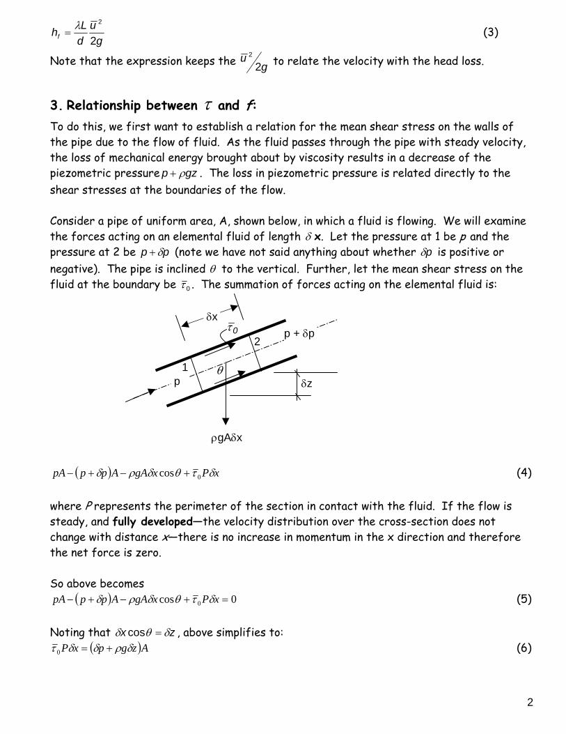
3. Relationship between τ and f: To do this, we first want to establish a relation for the mean shear stress on the walls of the pipe due to the flow of fluid. As the fluid passes through the pipe with steady velocity, the loss of mechanical energy brought about by viscosity results in a decrease of the piezometric pressure gzp ρ+ . The loss in piezometric pressure is related directly to the shear stresses at the boundaries of the flow. Consider a pipe of uniform area, A, shown below, in which a fluid is flowing. We will examine the forces acting on an elemental fluid of length δ x. Let the pressure at 1 be p and the pressure at 2 be pp δ+ (note we have not said anything about whether pδ is positive or negative). The pipe is inclined θ to the vertical. Further, let the mean shear stress on the fluid at the boundary be 0τ . The summation of forces acting on the elemental fluid is:

( ) xPxgAApppA δτθδρδ 0cos +−+− (4) where P represents the perimeter of the section in contact with the fluid. If the flow is steady, and fully developed—the velocity distribution over the cross-section does not change with distance x—there is no increase in momentum in the x direction and therefore the net force is zero. So above becomes

( ) 0cos 0 =+−+− xPxgAApppA δτθδρδ (5) Noting that zx δθδ =cos , above simplifies to:

( )AzgpxP δρδδτ +=0 (6)

δx

δz 1

2

p

p + δp

ρgAδx

0τ

θ

3

For fluid of constant density, the right hand side of the equation is Aδp* where p*=p + ρgδz. In the limit as δx→0,

dxdp

PA *

0 =τ (7)

Note that the piezometric pressure is effectively constant over the cross-section. This follows from the fact that there is no net movement of fluid perpendicular to the main flow. Note also, that we are considering the mean shear stress 0τ . The equation will hold for conduits that do not have circular cross-sections and in which the stress may be varying around the perimeter. For circular cross-sections, the stress anywhere on the perimeter is the same. Thus, the “bar” can be dropped from the equation above. This equation becomes:

dxdpR

dxdp

RR **2

0 22==

ππτ (8)

Similar derivation can be applied to a smaller, concentric, cylinder of fluid having radius r. Under the same conditions of fully developed steady flow, the equation (8) above may be written as:

dxdpr *

2=τ (9)

This equation says that the internal shear stress varies with the distance r from the pipe’s central axis. From equation (8) and (9) we get:

Rr

Rr

00

ττττ

=⇒= (10)

The distribution of stress is as follows: Pipe section of Radius R with fluid flowing within. Shear stress distribution From the above relations, we want to develop a relation between the stress at the boundary and the friction factor. From the definition of fh as defined in (1) above, the following can be written:

fhgp δρδ =− * (11) since

gph f ρ

*∆=

At r = R 0τ

r = 0 R r τ at r = r

4

And so,

gmdxdp

gdxdh f

ρτ

ρ0

*1−=−= (12)

Now,

gu

mf

xh

gu

mflh f

f 22

22

=→=δ

δ (13)

xh

ugmf f

δδ

2

2= (14)

2

002

21

2

ugmugmf

ρ

τρτ

−=−= (15)

We are interested in the magnitude of the friction factor and so the modulus of the shear stress is taken, giving:

2

0

21 u

fρ

τ= (16)

But how do we measure f. Reynolds reasoned that f depends on relative roughness of the pipe d

k or ( )dor ε where k

or ( )εor is the average roughness height and d is the pipe diameter. Dimensional analysis shows that f is a function of roughness d

k and Reynolds number, Re.

4. Variation of Friction Factor Derivation of an expression for friction factor in laminar flow Recall from treatment of laminar flow that:

( )*2

*1

4

8pp

LRQ −=µ

π (17)

( )fghL

RQ ρµ

π8

4

= (18)

gRLu

gRQLhf ρ

µρπµ

2488

== (19)

But from above ⎟⎟⎠

⎞⎜⎜⎝

⎛==

∆=

gu

mfL

gu

dfL

gphf 22

4 22*

ρ

5

gRLu

uLgdh

uLgdf f ρ

µ222

842

42

== (20)

Re16µ

=f (21)

Estimating f for turbulent flow Nikuradse’s experiments conducted in 1933 on roughness d

k

Discussion on the friction in pipes according to the Moody Diagram. Note the following regions:

• Laminar portion of the diagram according to the equation derived above • Smooth zone before the curve separates from the smooth pipe curve. • Transition zone • Rough zone where the friction factor is independent of Re.

Laminar Sub-Layer

Refer to Page 12. In the smooth zone the roughness height is within the viscous sub-layer and the pipe behaves like a smooth pipe. In the rough zone, the roughness extends outside the sub-layer and the pipe ceases to behave as a smooth pipe. The turbulent flow around each bump generates eddies in the wake giving rise to form drag. The energy loss is proportional to 2u . In this zone, viscous effects are negligible so that

2uhf ∝ so f is constant. A smooth surface may therefore be defined as one for which the roughness elements are so far submerged in the viscous sub-layer as to have no effect on the flow. A surface may therefore be smooth at a low Reynolds number but rough at a high Reynolds number. Nikuradse’s experiments were based on uniform roughness height and spacing which most often are not the case for actual pipes. At high enough Reynolds numbers, however, real pipes have a friction factor independent of Reynolds number and equivalent roughness height k may be determined experimentally. Such a figure was developed by Moody. This is widely used for predicting values of f.

6

For example, uncoated cast iron pipe: k = 0.25 mm; galvanized steel: k = 0.15 mm; drawn brass: k = 0.0015 mm Empirical formulae have been developed to describe parts of Moody’s diagram:

• Blasius Equation for the smooth pipe curve:

( ) 41

Re079.0 −=f (22)

• Haaland developed a formula which gives f for a large range of dk and Re:

⎪⎭

⎪⎬⎫

⎪⎩

⎪⎨⎧

⎟⎠⎞

⎜⎝⎛+−=

1.1

10 71.3Re9.6log6.31

dk

f (23)

So once f is determined, the head loss is given by:

gu

dL

gu

dfLhf 22

4 22 λ==

Note that Moody’s curves allow a computation of fh for a given Q directly. However, if p∆ or fh is given an iterative method has to be employed for determining Q as follows:

1. Estimate a value of f from the curve. 2. Calculate u from equation 3. Calculate Re 4. Refer to Moody’s curve for a new approximation of f 5. Repeat 1 to 4 until there is negligible change between successive estimates of f.

5. Friction in Non-Circular Pipes (conduits) For non-circular conduits experiments have shown that (in many cases) equations derived for circular pipes may be used. An equivalent diameter may be taken such that the hydraulic mean depth (radius) m is the same:

mdeq 4= (24)

where perimeterwetted

areawettedP

Am ==

This assumption works well for shapes that approximate a circle. For example, a square, oval, or equilateral triangle.

7

For rectangular ducts, the length should be less than 8 times the width. This equivalence concept does NOT apply to laminar flow. 6. Other Head Losses Losses have been found (through experiments) to vary with the square of the mean velocity

g2ukh,LossHead

2

f = (25)

Abrupt Enlargement See diagram on Page 13 below: The following is assumed:

− The velocity and pressure are uniform across the cross-section − Shear forces are neglected − p΄=p1

Net force to right is:

( ) ( )12221211 uuQApAApAp −ρ=−−′+ (26) Now 1pp ≈′ (27) So,

( ) ( )12221 uuQApp −ρ=− (28)

( ) ( )122

21 uuAQpp −ρ=− (29)

( ) ( )12221 uuupp −ρ=− (30)

From energy equation—note not Bernoulli’s as frictional losses are not negligible:

2

222

l1

211 z

g2u

gphz

g2u

gp

++ρ

=−++ρ

(31)

g2uu

gpph

22

2121

l−

+ρ−

= (32)

8

( )

g2uu

guuuh

22

21122

l−

+−

= (33)

( )g2uuh

221

l−

= (34)

From continuity

2211 uAuA = (35) Therefore,

2

1

222

2

2

121

l 1AA

g2u

AA1

g2uh ⎟⎟

⎠

⎞⎜⎜⎝

⎛−=⎟⎟

⎠

⎞⎜⎜⎝

⎛−= (36)

Note that hl for abrupt enlargement tends to g2

u21 as ∞→2A

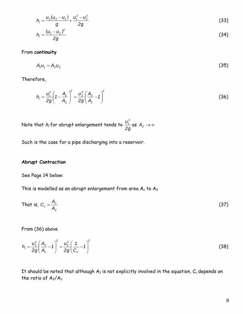
Such is the case for a pipe discharging into a reservoir. Abrupt Contraction See Page 14 below: This is modelled as an abrupt enlargement from area Ac to A2

That is, 2

cc A

AC = (37)

From (36) above

2

c

22

2

c

222

l 1C1

g2u1

AA

g2uh ⎟⎟

⎠

⎞⎜⎜⎝

⎛−=⎟⎟

⎠

⎞⎜⎜⎝

⎛−= (38)

It should be noted that although A1 is not explicitly involved in the equation, Cc depends on the ratio of A2/A1.

9

The table below gives some typical values for k (g2

ukh22

l = ) at various ratios of A2/A1

D2/d1 0 .2 .4 .6 .8 1 K 0.5 0.45 0.38 0.28 0.14 0.0

Also see Section 7.6.2 in Massey. Diffusers Reduces the velocity gradually, thus eliminating eddies. See Massey, 7.6.3. Losses in Bends Note that the head loss associated with a bend is given by:

g2ukh

22

l = (25)

Loss in Fittings and Valves Fittings are used to direct the path of flow or cause a change in the size of the flow path. These include elbows, tees, reducers, nozzles and orifices. Valves are used to control the amount of flow and may be globe valves, angle valves, gate valves, butterfly valves, check valves, etc. Energy loss incurred as fluid flows through a valve or fitting is computed using the Darcy

equation (Equation (1),g2

udfl4

gph

2*

f =ρ∆

= ).

However, the method of determining the resistance coefficient K is different. The value of k is reported in the form:

λ⎟⎠

⎞⎜⎝

⎛=DL

k e (41)

The ratio Le/D, called the equivalent length ratio, is considered to be constant for a given type of valve or fitting. Typical values are shown in the table below. The value of Le itself is called the equivalent length and is the length of straight pipe of the same nominal diameter as the valve (or fitting) that would have the same resistance as the valve (or fitting). The term D is the actual internal diameter of the pipe. (Remember that f4=λ )

EQUIVALENT

10

TYPE

LENGTH IN PIPE DIAMETERS, Le/D

Globe valve—fully open 340 Angle valve—fully open 150 Gate valve—fully open

¾ open ½ open ¼ open

8 35 160 900

Check valve—swing type 100 Check valve—ball type 150 Butterfly valve—fully open 45 90 standard elbow 30 90 long radius elbow 20 90 street elbow 50 45 standard elbow 16 45 street elbow 26 Close return bend 50 Standard tee—with flow through run

With flow through branch 20 60

7. Total Pressure Losses So far, the consideration has been on determining the individual head losses associated with friction losses along a length of pipe and minor losses due to bends, entry and exit into larger or smaller pipe sections, valves and fittings. Here, consideration is given to what real pipe systems may resemble. These systems consist of various lengths of pipes and combinations of devices for measuring flow rates, for controlling flow rates, changing flow directions, increasing flows from other sources or reducing the flows along the pipe system. This topic utilizes what has been done in earlier lectures. The hydraulic grade line (HGL) in a piping system is formed by the locus of points located a distance p/ρg above the centre of the pipe, or p/ρg + z above a pre-selected datum. The liquid in a piezometric tube will rise to the HGL.

The energy grade line (EGL) is formed by the locus of points a distance g

u2

2

above the HGL,

or the distance g

vu2

2

+ p/ρg + z above the datum. The liquid in a pitot tube will rise to the

EGL. Note the following points in relating the HGL with the EGL:

− As the velocity goes to zero the HGL and the EGL approach each other.

11

− EGL and, consequently, the HGL slope downward in the direction of the flow due to the head loss in the pipe. The greater the loss per unit length, the greater the slope. As the average velocity in the pipe increases, the loss per unit length increases.

− A sudden change occurs in the HGL and the EGL whenever a loss occurs due to a sudden geometry change.

− A jump occurs in the HGL and the EGL whenever useful energy is added to the fluid as occurs with a turbine.

− At points where the HGL passes through the centerline of the pipe, the pressure is zero. If the pipe lies above the HGL, there is a vacuum in the pipe, a condition that is often avoided if possible, in the design of piping systems. An exception would be in the design of a siphon.

12

δve

LaminarSub-

eδv

(a) Smooth pipe

(b) Rough pipe

Rough and Smooth Pipes

13

u1 u2

P1 A1

P2 A2D

FG

B

C

E

Head Loss at Abrupt Enlargement

14

u2u1

A2

A1

Area, Ac 1

2

Head Loss at Abrupt Contraction