experimental investigation of turbulent flow … · experimental investigation of turbulent flow...
TRANSCRIPT
i
NASA Technical Memorandum 105210
Experimental Investigation of Turbulent Flow
Through a Circular-to-RectangularTransition Duct
David O. Davis .......
Lewis Research Center
Cleveland, Ohio _ " ..... - -
_(_'ASA-T>4-1052!O) EXPERIMENTAL INV_STIC_ATION N91-31100
:JF TUR_.JLE-t-_T _=LL.-IW THRQUGH A
CIF<CULAR-TO-RE-CTANGULA_ TRANSITION DUCT
Ph.n. rhe,_is - Washington Univ. (t_ASA) Uncl_s
217 p CSCL OIA G3/02 0040346
-SePtem-1)er199 i ................................................................
https://ntrs.nasa.gov/search.jsp?R=19910021792 2018-08-28T11:46:06+00:00Z
EXPERIMENTAL INVESTIGATION OF TURBULENT FLOW THROUGH A
CIRCULAR-TO-RECTANGULAR TRANSITION DUCT
David O. Davis
National Aeronautics and Space Administration
Lewis Research Center
Cleveland, Ohio 44135
ABSTRACT
Steady, incompressible, turbulent, swirl-free flow through a circular-to-
rectangular transition duct has been studied experimentally. The transition duct
has an inlet diameter of 20.43 cm, a length-to-diameter ratio of 1.5, and an exit
plane aspect ratio of three. The cross-sectional area remains the same at the exit
as at the inlet, but varies through the transition section to a maximum value ap-
proximately 15e_ above the inlet value. The cross-sectional geometry everywhere
along the duct is defined by the equation of a superellipse. Mean and turbulence
data were accumulated utilizing pressure and hot-wire instrumentation at five
stations along the test section. Data are presented for operating bulk Reynolds
numbers of 88,000 and 390,000. Measured quantities include total and static
pressure, the three components of the mean velocity vector and the six compo-
nents of the Reynolds stress tensor. The results show that the curvature of the
transition duct walls induces a relatively strong pressure-driven crossflow that
produce a contra-rotating vortex pair along the diverging side-walls of the duct.
The vortex pair significantly distorts both the mean flow and turbulence field.
Local equilibrium conditions at the duct exit, if they exist at all, are confined to
a very small region near the wall indicating that care must be taken when using
wall functions to predict the flowfield. Analysis of the Reynolds stress tensor
at the exit plane shows that streamline curvature and lateral divergence effects
distort the non-dimensional turbulence structure parameters.
In addition to the transition duct measurements, a hot-wire technique which
relies on the sequential use of single rotatable normal and slant-wire probes has
been proposed. The technique is applicable for measurement of the total mean
velocity vector and the complete Reynolds stress tensor when the primary flow is
arbitrarily skewed relative to a plane which lies normal to the probe axis of rota-
tion. Measurement of the mean flow has been verified in fully-developed pipe flow
under simulated pitch angles up to 4-20 ° . Measurements of the Reynolds stress
tensor has been verified for the unskewed condition. Under skewed conditions,
systematic deviations of the stress tensor were observed which are attributed to
the geometry of the slant-wire probe. A new slant-wire probe is proposed which
is designed to reduce, if not eliminate, the observed deficiencies.
TABLE OF CONTENTS
Page
LIST OF FIGURES ..................................................... v
LIST OF TABLES .................................... . .................. x
NOMENCLATURE ...................................................... xi
CHAPTER 1 INTRODUCTION ....................................... 1
CHAPTER 2 PREVIOUS WORK ..................................... 7
CHAPTER 3 EXPERIMENTAL PROGRAM ......................... 15
3.1 Introduction .................................................. 15
3.2 Flow Facility .................................................. 15
3.3 Test Section .................................................. 16
3.4 Instrumentation ............................................... 17
3.5 Data Reduction ............................................... 18
CHAPTER 4 INLET CONDITIONS (Developing Pipe Flow) .......... 31
4.1 Introduction ................................................... 31
4.2 Preliminary Results ........................................... 32
4.3 Range of Operating Conditions ................................ 32
4.4 Results and Discussion ........................................ 33
CHAPTER 5 RESULTS AND DISCUSSION .......................... 47
5.1
5.2
5.3
5.4
5.5
5.6
5.7
CHAPTER 6
Introduction .................................................. 47
Static Pressure Distributions .................................. 47
Effect of Varying Reynolds Number ........................... 48
Mean Flow Results ............................................ 49
Turbulence Results ............................................ 53
Turbulence Modelling Considerations .......................... 59
\Vall Function Behavior ....................................... 63
CONCLUSIONS AND RECOMMENDATIONS ........ 125
PA_ l[ INTENTIONALLY BLANK °,.
]11PRECEDING PAGE BLANK NOT FILMED
REFERENCES ........................................................
APPENDIX A
APPENDIX B
APPENDIX C
APPENDIX D
APPENDIX E
APPENDIX F
APPENDIX G
129
Transition Duct Geometry ............................ 135
Hot-Wire Data Acquisition System .................... 139
Hot-Wire Techniques ................................. 145
Supplementary on Mean Flow Equation Development . 171
Supplementary on Turbulence Equation Development . 179
Verification of the Hot-Wire Technique ................ 187
Uncertainty Estimates ................................ 209
iv
LIST OF FIGURES
Page
1.1 Schematic of typical propulsion system ............................... 3
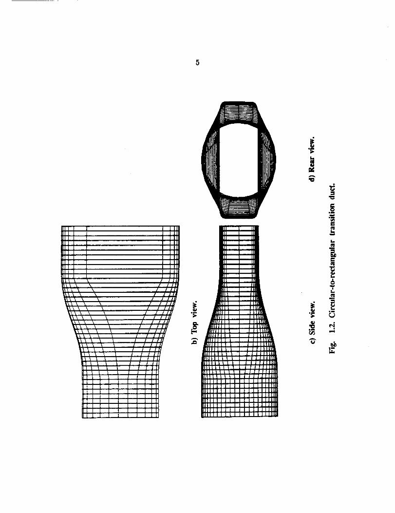
1.2 Circular-to-rectangular transition duct ............................... 4
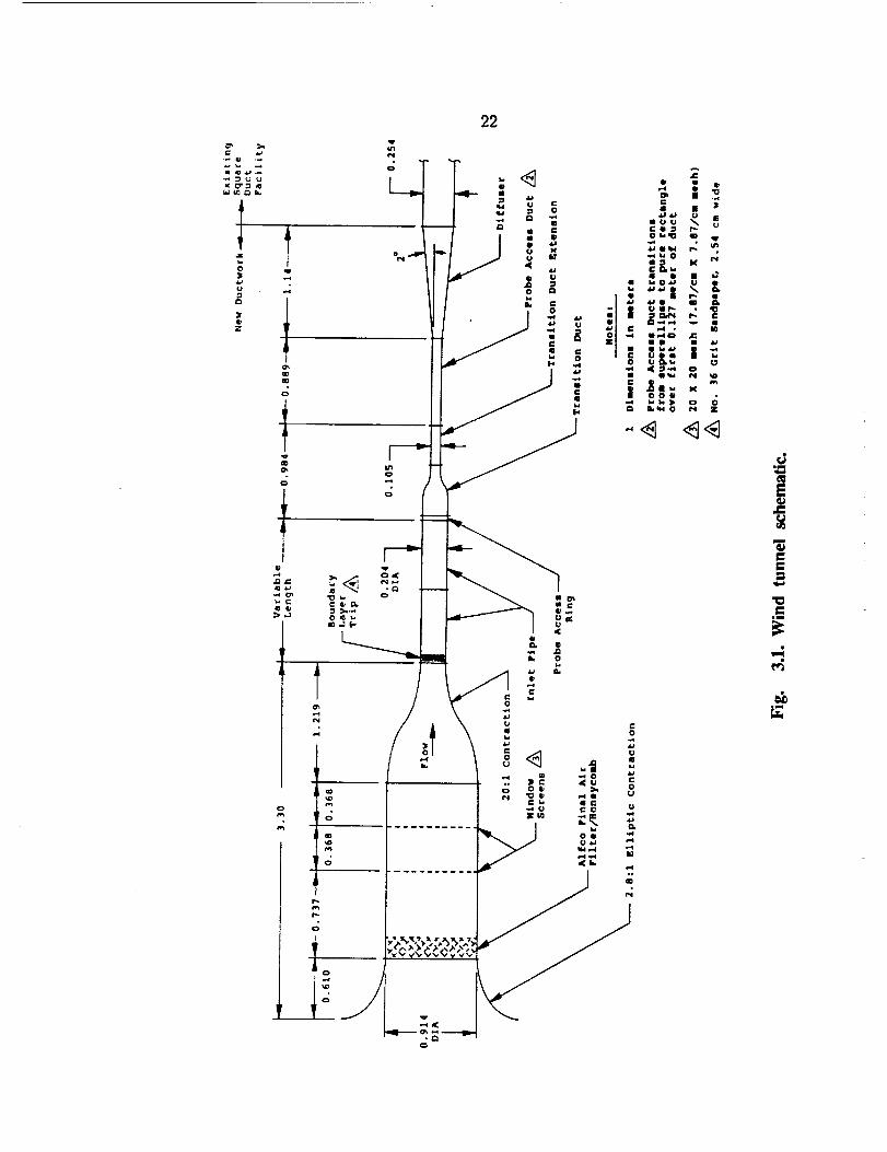
3.1 Wind tunnel schematic .............................................. 22
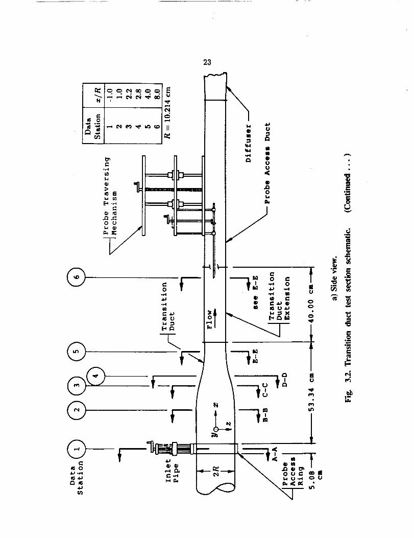
3.2 Transition duct test section schematic ............................... 23
3.3 Transition duct data stations ........................................ 29
4.1 Tripped and non-tripped boundary layer profiles at
Station I, Reb = 234,000 and 403,000 ............................... 38
4.2 Friction velocity vs. centerline Reynolds number at Station 1 ........ 39
4.3 Tripped boundary layer profiles at Station 1,
Reb "-- 52,000 and 88,000 ............................................ 40
4.4 Boundary layer profiles at Station 1, Reb -- 88,000 .................. 41
4.5 Boundary layer profiles at Station 1, Reb = 390,000 ................. 42
4.6 Reynolds stress distributions at Station 1 ............................ 43
4.7 Turbulence kinetic energy distributions at Station 1 ................. 44
4.8 Production of turbulence kinetic energy
distributions at Station 1 ........................................... 44
4.9 Shear stress correlation (Ruv = _"_/u_v t ) at Station 1 ................ 45
4.10 Shear-energy ratio parameter (al = _-d/2k) at Station 1 ............. 45
5.1 Peripheral wall pressure coefficient distributions ..................... 66
5.2 Total pressure contours at Station 5 ................................. 67
5.3 Axial mean velocity contours at Station 5 ........................... 68
5.4 Transverse mean velocity vectors at Station 5 ....................... 69
V
5.5 Total pressure contours ............................................. 70
5.6 Axial mean velocity contours ........................................ 73
5.7 Transverse mean velocity vectors .................................... 76
5.8 Static pressure contours at Station 5 ................................ 79
5.9 Axial distribution of strength of divergence parameter ............... 80
5.10 Surface oil flow visualization by Reichert [4] ......................... 80
5.11 Total pressure profiles along the semi-major
and semi-minor axes ................................................ 81
5.12 Axial mean velocity profiles along the semi-major
and semi-mlnor axes ................................................ 82
5.13 Axial mean vorticity contours ....................................... 83
5.14 Axial turbulence intensity contours .................................. 86
5.15 _'i/U_ x 104 Reynolds stress contours .............................. 87
5.16 v'-i/U_ x 104 Reynolds stress contours ............................... 88
5.17 -w--¢/U_ × 104 Reynolds stress contours .............................. 89
5.18 _-_/U_ x 104 Reynolds stress contours ............................... 90
5.19 _-_/U_ × 104 Reynolds stress contours .............................. 91
5.20 _-_/U_ × 104 Reynolds stress contours ............................... 92
5.21 Axial and transverse normal stress anisotropy (u 2 - v 2) .............. 93
5.22 Axial and transverse normal stress anisotropy (u 2 - w 2) ............. 94
5.23 Transverse normal stress anisotropy (v 2 - w 2) ....................... 95
5.24 Turbulence kinetic energy contours .................................. 96
5.25 Production of turbulence kinetic energy contours .................... 97
5.26 Reynolds normal stress profiles at Station 1 ......................... 98
vi
5.27 Normal stressprofiles alongsemi-major axis
at Stations 5 and 6 ................................................. 99
5.28 Shearstressand kinetic energyprofiles along semi-major axis ....... 100
5.29 Normal stressprofiles alongsemi-minor axis
at Stations 5 and 6 ................................................. 101
5.30 Shearstressand kinetic energyprofiles along
semi-minor axis, Reb=390,000 ...................................... 102
5.31 Shear stress and kinetic energy profiles along
semi-minor axis, Reb=88,000 ....................................... 103
5.32 Primary rates-of-strain at Station 5 ................................ 104
5.33 Component eddy viscosity distributions at Station 5 ................ 105
5.34 Primary rates-of-strain at Station 6 ................................ 106
5.35 Component eddy viscosity distributions at Station 6 ................ 107
5.36 Shear stress correlation (Ru_ = _"fi/u'v' ) ........................... 108
5.37 Shear stress correlation (Ruw = _'_/u_w ' ) ......................... 109
5.38 Shear stress correlation (R,_w = _"_/v'w _ ) .......................... 110
5.39 Shear-energy structure parameter (aly = x/h-'fi2 + b--_2/2k) .......... 111
5.40 Shear-energy structure parameter (alz = x/h'_ 2 + v'-w2/2k) ......... 112
5.41 Physical realizability limits of turbulence invariant map ............ 113
5.42 Anisotropic stress tensor invariants at Station 1 .................. .. 114
5.43 Anisotropic stress tensor invariants at Station 5 .................... 115
5.44 Anisotropic stress tensor invariants at Station 6 .................... 116
5.45 Reference coordinates for wall function behavior .................... 117
5.46 Peripheral skin friction coefficient distributions ..................... 117
5.47 Law-of-the-wall velocity profiles .................................... 118
vii
5.48 x/(_fi 2 -I-h-_2)/U_ distributions parallel to semi-minor axis ......... 119
5.49 k/U_ distributions parallel to semi-minor axis ...................... 120
5.50 Pyw/U_ distributions parallel to semi-minor axis ................... 121
5.51 x/(_'fi 2 + _'_2)/V2r distributions along semi-major axis .............. 122
5.52 k/U_ distributions along semi-major axis ........................... 122
5.53 Pyw/U_ distributions along semi-major axis ...., ................... 123
B.1 Block schematic of hot-wire data acquistion system ................. 144
C.1 Hot-wire probe configurations for Method A ........................ 164
C.2 Hot-wire positions for mean flow determination ..................... 165
C.3 Reference coordinates for Reynolds stress determination ............ 166
C.4 Behavior of Reynolds stress coefficients, normal-wire, Method A ..... 167
C.5 Behavior of Reynolds stress coefficients, slant-wire, Method A ....... 168
C.6 Behavior of Reynolds stress coefficients, normal-wire, Method B ..... 169
C.7 Behavior of Reynolds stress coefficients, slant-wire, Method B ....... 170
D.1 Effective cooling velocity for mean flow calculations ................ 176
D.2 Tangential cooling coefficient behavior ............................. 177
E.1 Effective cooling velocity for turbulence calculations ................ 185
F.1 Schematic of Method A hot-wire verification setup ................. 194
F.2 Hot-wire orientation for Method A ................................. 194
F.3 Typical probe construction for Method A .......................... 195
F.4 Detail of probe prong geometry for Method A ...................... 195
F.5 Offset prong slant-wire calibration ................................. 197
F.6 Conjectured probe prong influence for offset prong slant-wire ....... 197
F.7 Fully-developed mean flow for unskewed conditions ................. 198
o.°
VIII
F.8 Fully-developed pipe flow Reynolds stress profiles
for unskewed conditions ............................................ 199
F.9 Fully-developed mean flow for skewed conditions ................... 201
F.10 Transformed Reynolds stress profiles ............................... 203
F.11 Proposed offset prong slant-wire probe ............................. 908
F.12 Interference region for proposed slant-wire probe ................... 208
ix
LIST OF TABLES
Page
4.1 Boundary layer parameters at Station 1 ............................. 34
5.1 Velocity deficit in the vicinity of the vortex cores .................... 54
5.2 Normalized boundary layer thickness (_/R) at Stations 1,5 and 6 .... 57
5.3 Normalized friction velocity (U,./Ub x 100) at mid-planes, Reb=390,O00 58
A.1 Transition duct polynomial coefficients ............................. 136
A.2 Transition duct geometry variables ................................. 137
B.1 DMA Interface Cable pin connections .............................. 143
X
NOMENCLATURE
[ENGLISH SYMBOLS I
a = semi-major axis of superellipse
al
Ae8
AR
b
B
C
CI
CpC_,
d
D
e
E
EO
h
hBy
hN
H12
H32
k
k
kr
lp
L
Tn
n
P
P
= shear-energy ratio parameter (_--_/2k)
= transition duct cross-sectional area
= transition duct aspect ratio
= semi-minor axis of supereUipse
= slope of: calibration characteristic
= law-of-the-wall constant (5.0)
= skin friction coefficient (rw/(½pV_))
- P,)/ pvb)= pressure coefficient ((Pw 1 2
= empirical constant (0.09)
- Preston tube outside diameter
= transition duct inlet diameter
= fluctuating bridge voltage component
= instantaneous bridge voltage
= bridge voltage intercept at zero velocity
= dynamic pressure head (Pt - P)
= binormal cooling coefficient
= normal cooling coefficient
= first boundary layer shape factor (`51/`52)
= second boundary layer shape factor (,53/62)
= kinetic energy of turbulence
= tangential cooling coefficient
= reference tangential cooling coefficient
= Prandtl's length scale
= distance from begining to end of transition
= generalized cooling law exponent
= non-linearized cooling law exponent (0.45)
= static pressure
= production of turbulence kinetic energy
xi
P,
R
Rc
1:_u v
.Ru w
,tr_vw
Re
8
T
tll _ yt _W ¢
_2 _V2 _ W 2
_'-fi, _'-_ ,
U,V,W
U_
Ur
U,
Yr
X_ y_ Z
Xp
Xl, y_ Z I
X_ yl Z I
2w_ Yw_ Zw
= total pressure
1 prr2= reference dynamic pressure (_ v, )
= cylindrical (pipe) coordinates
- inlet pipe radius
= radius of curvature
- shear stress correlation (_-'fi/u'v I)
= shear stress correlation (_'_/u'w')
-- shear stress correlation (_-'_/v'w')
= Reynolds number (UD/v)
= peripheral curvilinearcoordinate (Fig.3.2)
= temperature ,
= rms Reynolds normal stresscomponents
= Reynolds normal stresscomponents
= Reynolds shear stresscomponents
= mean velocity components in the x, y, z-directions
= effective cooling velocity
= resultant yaw velocity vector in the x-z plane
= friction velocity (_)
= resultant transverse velocity vector in the y-z plane
= primary cartesian coordinate system
= streamwise coordinate measured from pipe inlet
= secondary cartesian coordinate system (Method A)
= secondary cartesian coordinate system (Method B)
= local wall coordinate system (yw normal to duct surface)
IGREEK SYMBOLS I
of
F
,5
,51
= angle between probe axis and wire normal
= flow angle (8 = tan-l(V/U))
= angle == Gamma function
= boundary layer thickness
= axisymmetric displacement thickness
xii
_2 = axisymmetric momentum thickness
_3 = axisymmetric energy thickness
Ap = Preston tube pressure head
e = dissipation rate of turbulence kinetic energy
= pitch flow angle (_ = tan-l(V/Ur))
7? = exponent of superellipse equation
0 = wire rotation angle (relative to secondary coordinates)
i¢ = Von Karman's constant (0.41)
A = wire rotation angle (relative to primary coordinates)
p = molecular viscosity
#t = turbulent viscosity
v = kinematic viscosity (#/p)
p = density
7"w = wall shear stress
¢ = total mean flow skewness angle
¢ = wire orientation angle
f/_ = mean streamwise vorticity (OW/Oy - OV/Oz)
[SUBSCRIPTS]
arnb = ambient condition
b = bulk condition
cI = centerline condition
FD = fully-developed condition
i = inlet condition
L = linearized quantity
N L = non-linearized quantity
BN = binormal effective cooling velocity component
N = normal effective cooling velocity component
P = parallel (tangential) effective cooling velocity component
n = normal-wire
s = slant-wire
w = wall condition
xiii
( )
ISPECIAL NOTATIONS]
= time-averaged quantity
xiv
; Z
CHAPTER 1
INTRODUCTION
The term "transition duct" refers to a class of internal flow configurations in
which the cross-secti0nal shape changes in the streamwise direction. Examples
include ducts which change cross section from square-to-round, round-to-square,
square-to-rectangular, etc. Transition ducts are commonly used in ventilation
systems, in aircraft propulsion systems, as wind tunnel components and as dif-
fusers in hydro-electric turbines. High-performance military aircraft often utilize
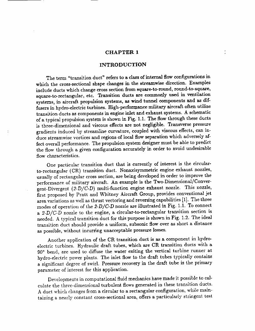
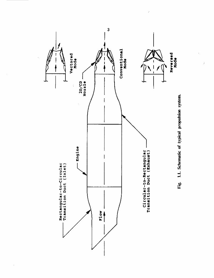
transition ducts as components in engine inlet and exhaust systems. A schematic
of a typical propulsion system is shown in Fig. 1.1. The flow through these ducts
is three-dimensional and viscous effects are not negligible. Transverse pressure
gradients induced by streamline curvature, coupled with viscous effects, can in-
duce streamwise vortices and regions of local flow separation which adversely af-
fect overall performance. The propulsion system designer must be able to predict
the flow through a given configuration accurately in order to avoid undesirable
flow characteristics.
One particular transition duct that is currently of interest is the circular-
to-rectangular (CR) transition duct. Nonaxisymmetric engine exhaust nozzles,
usually of rectangular cross section, are being developed in order to improve the
performance of military aircraft. An example is the Two-Dimensional/Conver-
gent-Divergent (2-D/C-D) multi-function engine exhaust nozzle. This nozzle,
first proposed by Pratt and Whitney Aircraft Group, provides conventional jet
area variations as well as thrust vectoring and reversing capabilities [1]. The three
modes of operation of the 2-D/C-D nozzle are illustrated in Fig. 1.1. To connect
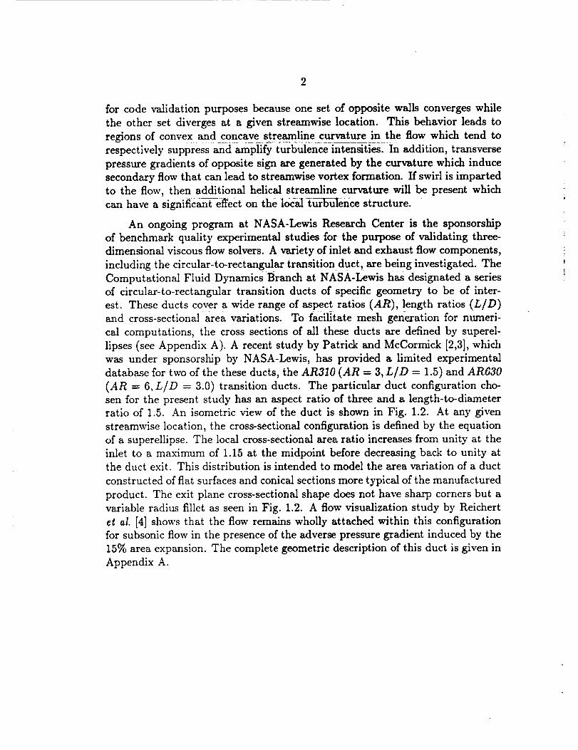
a 2-D/C-D nozzle to the engine, a circular-to-rectangular transition section is
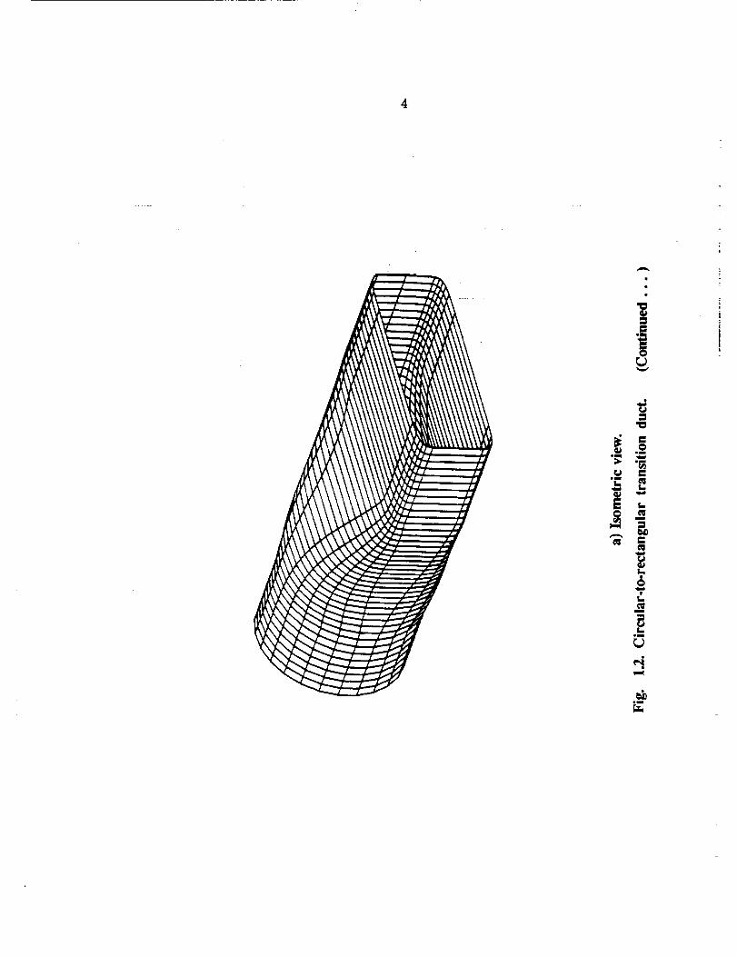
needed. A typical transition duct for this purpose is shown in Fig. 1.2. The ideal
transition duct should provide a uniform, subsonic flow over as short a distance
as possible, without incurring unacceptable pressure losses.
Another application of the CR transition duct is as a component in hydro-
electric turbines. Hydraulic draft tubes, which are CR transition ducts with a
90 ° bend, are used to diffuse the water exiting the vertical turbine runner at
hydro-electric power plants. The inlet flow to the draft tubes typically contains
a significant degree of swirl. Pressure recovery in the draft tube is the primary
parameter of interest for this application.
Developments in computational fluid mechanics have made it possible to cal-
culate the three-dimensional turbulent flows generated in these transition ducts.
A duct which changes from a circular to a rectangular configuration, while main-
taining a nearly constant cross-sectional area, offers a particularly stringent test
2
for code validation purposesbecauseone set of opposite walls convergeswhilethe other set divergesat a given streamwiselocation. This behavior leads toregions of convex and concavestreamline curvature in the flow which tend torespectively suppressand _plify turbulence intensities_In addition, transversepressuregradients of opposite sign aregeneratedby the curvature which inducesecondaryflow that can lead to streamwisevortex formation. If swirl is impartedto the flow, then additional helical streamline curvature will be present whichcan have a significant effecton the local tur_buIencestructure.
An ongoing program at NASA-Lewis ResearchCenter is the sponsorshipof benchmark quality experimental studies for the purposeof validating three-dimensionalviscousflow solvers.A variety of inlet and exhaustflow components,including the circular-to-rectangular transitionduct , arebeing investigated. TheComputational Fluid DynamicsBranch at NASA-Lewis has designateda seriesof circular-to-rectangular transition ducts of specific geometry to be of inter-est. Theseducts covera wide range of aspect ratios (AR), length ratios (L/D)and cross-sectionalarea variations. To facilltate mesh generation for numeri-cal computations, the crosssections of all these ducts are defined by superel-lipses(seeAppendix A). A recent study by Patrick and McCormick [2,3],whichwas under sponsorslfip by NASA-Lewis, has provided a limited experimentaldatabasefor two of the theseducts, the AR310 (AR = 3, LID = 1.5) and AR630
(AR = 6, L/D = 3.0) transition ducts. The particular duct configuration cho-
sen for the present study has an aspect ratio of three and a length-to-diameter
ratio of 1.5. An isometric view of the duct is shown in Fig. 1.2. At any given
streamwise location, the cross-sectional configuration is defined by the equation
of a superellipse. The local cross-sectional area ratio increases from unity at the
inlet to a maximum of 1.15 at the midpoint before decreasing back to unity at
the duct exit. This distribution is intended to model the area variation of a duct
constructed of flat surfaces and conical sections more typical of the manufactured
product. The exit plane cross-sectional shape does not have sharp corners but a
variable radius fillet as seen in Fig. 1.2. A flow visualization study by Reichert
et al. [4] shows that the flow remains wholly attached within this configuration
for subsonic flow in the presence of the adverse pressure gradient induced by the
15% area expansion. The complete geometric description of this duct is given in
Appendix A.
0
O_
UE0
: (JF-t\N
_0
o
C
uC
I ._Ou
I
,.-40
C.,4
utD
3
aco
_0
CO
0
J
\ll ®_=
1..iA
Uv
I {JO_
I,-,¢:aO
_M.,-0CU_
E.*
"E.
tm
i
!
om
s_
t_
6L
wm
H
5
1
I
\ \ \\
\
_..l i II/ # I1_
l, Ille
i,l
ill,
ICl
ill
em
t,#
I
i6
m
e,,,lum
e,,,9
1/
CHAPTER 2
PREVIOUS WORK
Turbulent flow through a circular-to-rectangular transition duct is character-
ized by streamline curvature and streamwise vorticity embedded in the boundary
layer. In addition, the boundary layer is subjected to both lateral convergence
and divergence. This chapter will begin by reviewing previous transition duct
studies, followed by a discussion of the effect that streamline curvature, embed-
ded vorticity and lateral divergence have on turbulent boundary layer flow.
2.1 Flow Through Transition Ducts
The earliest study on transition duct flow was an experimental investiga-
tion done by Mayer [5] in 1939. In his study, he investigated flow through
two rectangular-to-circular (and vice versa) transition ducts of constant cross-
sectional area. The ducts had transition lengths of 0.69 and 2.76 hydraulic diam-
eters. The data included streamwise static pressure distributions, total pressure
contours and the three-dimensional velocity field. In a similar study, Taylor et al.
[6] investigated turbulent flow through a square-to-round transition duct whichhad a 21.5% reduction in cross-sectional area over the length of the transition.
This decrease in area was the result of the hydraulic diameter (40 ram) being
held constant along the duct. The transition occurred over two hydraulic diam-
eters. LDV techniques were used to measure streamwise and transverse velocity
components along the duct for an operating Reynolds number of 35,350. The
results of these studies have shown that the length of the transition section is
influential on flow development and that pressure-driven crossflows (_ 10% of
maximum streamwise velocity), can lead to significant distortion of the primary
flOW.
During the early development stages of the 2-D/C-D nozzle, Pratt and Whit-
ney Aircraft developed a design procedure for circular-to-rectangular transition
ducts intended to minimize both pressure losses and axial length. This procedure
is governed by the following criteria [1]:
1) Constant cross-sectional area
2) Corner radius decreasing linearly with length
3) Straight sidewalls
4) Sidewall divergence angle limit = 45 degrees
In a recent combined experimental and numerical study by Burley et al. [7,8],
the original P\VA guidelines were examined to determine if expanded design
criteria could be established so that shorter transitions are possible, thereby
reducing exhaust system weight. Five different circular-to-rectangular transition

PRECEDI;'-;G PAGE BLANK NOT FILMED
duct configurations were investigated to explore the effects of duct length, wall
shape and cross-sectional area distribution on performance. All of the ducts
were defined by super-elliptic cross sections (see Appendix A). The transition
ducts were installed in a transonic wind tunnel with a high aspect ratio, non-
axisymmetric nozzle and the overall internal performance was measured. In
addition, one duct was tested with swirl vanes installed. Discharge coefficient
and thrust ratio versus n0zzle-pressure ratio were used as performance criteria.
The results of their innvest]-gat]on show that f_or length ratios less flaan or equal
0.75, large regions of separated flow are present. However, because the flow
reattached before the entrance to the n0zzle[only a Sm_decrease in performance
was observed. They also found that Swirling the fl0W: -had a positive effect on
performance for !ow nozzle pressure ratios, but that performance was decreased
when the nozzle was near a choked condition. Finally, these researchers reported
that decreasing the cross-sectional area along the duct reduced flow separation
and provided a modest increase in performance.
Patrick and McCormick [2,3] were the first to make turbulence measure-
ments within a circular-to-reCtangular tr_s_tlonduct.:LDV and total=pressure
measurements were made at the inlet and outlet stations of two different ducts
at an operating Reynolds number of 420,000. The first duct, designated the
AR310, had an aspect ratio of three,:a length-to-di_eter ratio of one, and con-
stant cross-sectional area through the duct. The second duct, designated the
AR630, had an aspect ratio of six and a length-to-diameter ratio of three. The
local cross-sectional area ratio increased from unity at the inlet to a maximum
of 1.10 at the midpoint before decreasing back to unity at the duct exit. In order
to facilitate grid generation for numerical comparisons, the cross-sectional shape
everywhere along the ducts was prescribed by the equation of a superellipse.
Measured quantities included all three mean velocity components and the three
normal Reynolds stress components at the inlet and outlet planes. The results
for the AR310 duct showed that the axial mean flow did not develop uniformly
but had a convex profile along the major axis at the duct exit plane. Outward
transverse velocities, nominally parallel to the major axis, were observed that
peaked at about 10% of the bulk velocity. No streamwise vorticlty was observed
except deep in the corner region, but the measurement grid was too coarse to
discern discrete vortical motion. The AR630 duct behaved quite differently. Here
the flow developed much more uniformly, and a pair of discrete vortices along
the duct sidewalls, centered about the duct semi-major axis, were observed. The
origin of these vortices is in the first half of the transition where the wall cur-
vature creates a pressure gradient which causes a crossflow from the upper and
lower walls to the sidewalls. The crossflow meets at the duct centerline and turns
inward along it. in the second half of the duct, where the curvature changes sign,
the pressure gradient is reversed, counteracting the secondary motion. If a vorti-
cal pattern was established in the first half of the AR310 duct, then the reversed
pressuregradient waseffective in stopping it.
Miau et al. [9] experimentally investigated three CR ducts with length-to-
diameter ratios of 1.08, 0.92 and 0.54, under low subsonic flow conditions. The
aspect ratio was equal to two and the cross-sectional area was constant for all
three ducts. Mean flow and turbulence data were taken at the inlet and exit
planes. Secondary flow patterns indicative of streamwise vortex formation were
observed at the exit plane of the ducts. Prom these results, all the terms in
the axial mean vorticity equation were computed. Their analysis showed that
the generation of streamwise vorticity is due primarily to transverse pressure
gradients induced by geometrical deformation.
With the exception of the performance data reported by Burley et al. [7,8],
none of the above studies considered the case where a swirl velocity component
is imparted to the inlet flow. The addition of swirl may have several benefits.
First, swirl will impart a radial velocity component to the flow, thus improving
it's ability to follow steeply sloped sidewalls in the transition duct. Secondly,
Schwartz [10] has observed that noise associated with axisymmetric jet exhaust
can be reduced by swirling the flow. Finally, in an axisymmetric jet, the rate
of decay of the axial velocity component can be substantially increased (reduced
thermal plume) by swirling the flow, with minimal loss of thrust [11]. Der et al.
[12] performed a water tunnel flow visualization study of swirling flow through a
CR duct. Later, Chu ef al. [13,14] analyzed these data and found that swirling
the flow dramatically reduced the thermal plume. Recently, Reichert et aI. [4],
using a duct identical to the one in the present study, compared the mean flow
field for the cases of swirling and non-swirling inlet flow at an operating Mach
number of 0.35 and a Reynolds number of 1.5 x l0 s.
Related studies have been undertaken which include the effects of a turbine
centerbody and axial centerline curvature. Sobota and Marble [15] performed a
detailed experimental and numerical investigation of a CR transition duct with a
large centerbody and various degrees of inlet swirl. This study provided insight
into vorticity generation mechanisms and the ability to tailor vorticity distribu-
tions. CR transition ducts with a 90 ° bend in the transition section (hydraulic
turbine draft tubes) have recently been analyzed with and without swirl by Vu
and Shyy [16]. The fiow through the draft tube was predicted using a finite-
volume approximation to the full Navier-Stokes equations in conjunction with a
k-e turbulence model and the results were compared to wind and water tunnel
experimental data. In general, pressure recovery, as well as the three-dimensional
velocity field, agreed well between experiment and numerical predictions.
The review of the literature has revealed that there is only a small experi-
mental database for flow through a circular-to-rectangular transition duct that is
of sufficient detail to be useful for CFD code calibration/validation purposes. At
the present, only Miau's data set include measurements of the complete Reynolds
10
stress tensor in a CR transition duct. The present study is intended to help fill
this void by providing complete mean flow and Reynolds stress measurements at
the inlet and outlet stations, supplemented by mean flow data at intermediate
stations, for a duct with an aspect ratio larger than that considered by Miau.
On the basis of previous work in this area, it was anticipated that skew induced
secondary flow would have a dominating influence on the primary flow and on
the local turbulence structure.
2.2 Streamline Curvature Effects
A great deal of work has been published on the effects of streamline curvatureon turbulent boundary layer development. Thebulk of the studies have been for
the quasi-two-dimensional case with the curvature induced by a constant radius
bend in a square or rectangular wind tunnel. Although the transition duct flow
is considerably more complex, it is useful to examine previous related results in
order to gain some insight into the mechanisms operating within the transitionduct.
In 1973, Bradshaw [17] pubhshed a comprehensive review of the effects of
streamline curvature on turbulent flow. His work was moti_ted by what he
referred to as "the surprisingly large effect exerted on shear'flow turbulence by
curvature of the streamlines in the plane of the mean shear". Flows with stream-
line curvature are characterized by the presence of extra rates of strain, that is,
rates additional to the simple shear aU/Oy. When the equations of motion are
written in semi-curvilinear coordinates (e.g., the s,n system of reference [17]),
extra explicit terms appear which account for the presence of curvature. Ex-
perimental measurements have shown, however, that the effects of extra rates
of strain are an order of magnitude larger than would appear when calculation
methods for simple shear flows are extended to curved flows. Bradshaw explains
this discrepancy by concluding that streamline curvature directly causes large
changes in the higher-order parameters of the turbulence structure.
Convex and concave curvature are often referred to as stabilizing and desta-
bilizing curvature, respectively. Laminar flow over a destabilizing (concave) sur-
face is subject to centrifugal instability which is characterized by the presence
of streamwise vortices within the boundary layer; the so-called Taylor-GSrtler
vortices. For turbulent flows over a concave surface, the presence of vortices
analogous to the laminar Taylor-GSrtler type have been observed experimentally
by So and Mellor [18,19], Meroney and Bradshaw [20] and Hoffmann et al. [21],
as well as others; and numerically, by direct simulation of the Navier-Stokes
equations, by Moser and Moin [22]. In addition, the stabilizing and destabilizing
effect on turbulence acts, respectively, to attenuate and amplify the turbulence
intensities.
i
i
|i|!!!
11
In regions sufficiently close to curved walls, mean velocity profiles have been
observed to follow the flat plate law-of-the-wall for both convex and concave
curvature [18,19,23]. Hoffman and Bradshaw [24] have suggested that the law-
of-the-wall applies when y/Rc is small. This is important in that it allows for the
use of law-of-the-wall based wall functions in numerical computations. The agree-
ment with law-of-the-wall behavior is apparently where the similarity between
convex and concave curved flows end. In contrast to flat plate flows, turbulent
flow over a convex surface is characterized by slower boundary layer growth, lower
wall shear stress, reduced turbulence intensities and reduced heat transfer rates.
Conversely, turbulent flow over a concave surface is characterized by increased
boundary layer growth, higher wall shear stress, increased turbulence intensities
and increased heat transfer rates, as well as the aforementioned streamwise vor-
tices. The most significant difference in the turbulence statistics appears in the
Reynolds shear stress. Measurements by So and Mellor [18], Gillis and Johnston
[25] and Smits et al. [26] show a sharp decrease in the turbulent shear stressto near-zero levels in the outer region of the boundary layer when a flat plate
boundary layer is suddenly subjected to a strong (_5/Rc w, 0.10) convex curvature.
For the concave case, the turbulent shear stress dramatically increased to a near
two-fold level as compared to flat plate results. Hunt and Joubert [27] found
similar behavior in flows subjected to mild streamline curvature (_5/Rc w, 0.01),
but to a lesser degree. The two flow cases also respond differently when they are
subjected to a flat plate recovery region. Whereas the Reynolds stresses recover-
ing from convex curvature do so in a monotonic fashion, the stresses in concave
flows drop well below their entry region values before recovering [26].
The dramatic differences between the convex and concave curvature cases
have hindered development of adequate turbulence models because the mecha-
nisms that produce them are not well understood. Indeed, Muck et al. [28] have
concluded that, although governed by the same dimensional analysis, there is
no other useful connection between the two cases. From this conclusion, they
imply that allowances for the effect of streamline curvature in calculation meth-
ods for turbulent flows should be formulated separately for the stabilizing and
destabilizing cases.
The above discussion serves to illustrate factors which may add to the com-
plexity of transition duct flow. The degree to which streamline curvature affects
transition duct flow depends on the thickness of the incoming boundary layer.
For the present study, a boundary layer thickness of i_/R ,_ 0.25 is anticipated.
This corresponds to a maximum curvature parameter of _/Rc _ 0.085 for both
convex and concave walls. On the basis of previous experimental results, it was
expected that streamline curvature would influence the development of the flow
in the transition duct.

12
2.3 Embedded Streamwise Vortices
The transition duct studies reported in Refs. 2,3 and 9 have shown that
streamwise vorticity is generated within CR transition ducts. The results for
the AR630 duct (Refs. 2 and 3) show that a discrete vortex pair (common flow
away from the surface) develops in the duct sidewall boundary layer. Stream-
line vortices embedded in a boundary layer are-as-often beneficial as they axe
detrimental. On aircraft flight surface_s,_ strearnwise vortices are purposefully
generated to promote mixing between the freestream and the boundary layer in
order to forestall flow separation. In eombustor applications, streamwise vor-
tices are used to enhance mixing between fuel and oxidant. In turbomaehinery,
however, streamwise vortices generated by blade-hub junctures may sweep away
the protective film cooling on adjacent blades causing damaging hot spots. In
transition duct applications, streamwise vortices result in undesirable pressure
losses, although they may inhibit flow separation.
Streamwise vortices in boundary layers can be generated by transverse pres-
sure gradients or by gradients of the Reynolds stresses. Pressure-gradient induced
streamwise vorticity occurs whenever a shear layer (laminar or turbulent) with
spanwise vorticity is deflected laterally by transverse pressure forces. If the de-
flection occurs over a short spanwise distance, then a discrete vortex is formed.
Vortices generated in this manner occur in strut-endwall (junction) configura-
tions and in flow through curved ducts. Reynolds stress induced vorticity occurs
in turbulent flow through non-circular ducts, even when the ducts are straight,
i.e., uncurved in the streamwise direction. Because both types of vorticity gener-
ation occur in many practical engineering flows, a large body of literature exits
on the subject. Some of the more comprehensive experimental studies on the
effect that embedded streamwise vortices have on the mean flow and turbulence
structure include those due to Shabaka et al. [29], Mehta and Bradshaw [30]
and Pauley and Eaton [31,32]. These researchers studied the effects of single
and paired vortices in an otherwise two-dimensional boundary layer flow. Mean
flow and turbulence (one-point double and triple correlations) were measured.
The vortices in all these studies were generated by half-delta wings, although
the placement of the generators in the wind tunnels differed. Whereas Pauley
and Eaton placed the generators on the floor of the 2-D channel, Shabaka and
Mehta placed the generators upstream of the contraction in the settling chamber.
By placing the generators in the plenum, the velocity deficit in the wake of the
delta wing is reduced to a small percentage of the freestream velocity as the flow
accelerates through the contraction. Pauley and Eaton obtained data in measure-
ment planes 97 and 188 cm downstream from the generators. Shabaka and Mehta
present results in measurement planes between 60 and 255 cm downstream. The
results of these investigations showed that thickening of the boundary layer oc-
curred in upwash regions and thinning occurred in downwash regions. Paired
vortices with the common flow away from the surface were attracted and moved
13
away from the surface. In contrast, vortex pairs with the common flow towards
the surface moved away from each other and stayed in close proximity to the
wall. In the vicinity of the vortex core(s), a concentrated maxima of turbulence
intensity occurs, but no large-scale unsteadiness in the flow was detected. When
compared to the surrounding 2-D boundary layer, large changes in the dimen-
sionless turbulence structure parameters were observed and eddy viscosities were
reported to be very ill-behaved in the vortex region. These observations led the
researchers to conclude that full Reynolds stress transport modelling would be
required for prediction purposes.
Liandrat et al. [33] used the data of Refs. 29 and 30 for comparison with
numerical simulations based on mixing length and k-e turbulence models. In
addition, calculations based on two forms of the Reynolds stress transport equa-
tions were performed. The results of this investigation showed simple turbulence
models provide good estimations of overall mean flow properties for the case of a
single embedded vortex. For the case of paired vortices with common flow away
from the surface, the mean flow results were found to be largely unsatisfactory.
For both cases, details of the predicted turbulence structure required Reynolds
stress transport models. However, even these higher-order models did not give
adequate predictions of the transverse normal stresses and the secondary shear
stresses that control the diffusion of streamwise vorticity. In a review of turbu-
lent secondary riows, Bradshaw [34] concludes that the primary inadequacy in
the Reynolds stress transport models is in the modelling of the pressure-strain
term.
As a final note, Patrick and McCormick [2,3] made mention of the similarity
between the generation of the vortex pair in the AR630 CR transition duct and
in a circular pipe with an S-shaped bend. Experimental mean flow results and a
discussion of vorticity generation for the latter case is presented by Bansod and
Bradshaw [35]. Limited turbulence measurements in a circular S-shaped duct
with embedded vortices are presented by Taylor et aI. [36].
2.4 Laterally Diverging Boundary Layer
Along the converging walls of a CR transition duct, the boundary layer is
subjected to lateral divergence. Conversely, along the diverging walls, the bound-
ary layer converges laterally. Boundary layer divergence is another example of a
shear flow with extra strain rates (OV/Oy, OW/Oz). As in the case of streamline
curvature, the effect that lateral divergence has on the turbulence structure of a
boundary layer is much larger than, and sometimes opposes, what is predicted
by explicit terms that appear in the Reynolds stress transport equations. The
strength of divergence in a boundary layer is typically characterized by the rate-
of-strain parameter (OW/Oz)/(OU/Oy). Smits et al. [37] reviewed the effect that
lateral divergence and convergence have on boundary layer flow. In addition,
14
they obtained mean flow and turbulence measurements in a diverging boundary
layer that develops on a cylinder-flare where ((OW/Oz)/(OU/Oy) ,_ 0.1) midwaythrough the layer. In the transition region between the cylinder and flare, the
flow was subjected to relatively strong concave iongitud'maI curvature. Although
they found that the effects of divergence and curvature in the transition region
could not be quantitatively separated, they argue that the memory of the cur-
vature is short-lived and that the downstream flowfield is primarily a result of
divergence effects alone. They note that boundary layers subjected to lateral
divergence and convergence tend to, respectively, thin and thicken. Turbulence
kinetic energy is amplified for the diverging case and attenuated for the converg-
ing case. The shear stress in a diverging boundary layer is elevated and a peak
occurs which moves outward from the surface as the flow develops. Pauley and
Eaton [31,32] obtained mean flow and turbulence measurements in the diverging
boundary layer that develops between an embedded vortex pair with the com-
mon -.flow towards the surface. Although the strength of divergence was fairly
weak ((OW/az)/(OU/ay) _ 10-3), the flow is unique, inasmuch as complicating
factors such as streamwise pressure gradients and curvature are absent. Unlike
the results of Stairs (and others), these researchers found no significant differ-
ence in either the mean flow or the Reynolds stresses when compared to their
counterparts in the two-dimensional boundary layer outside the vortex pair.
2.5 Concluding Remarks
Turbulent flow through a circular-to-rectangular transition duct represents
a practical engineering flow of interest where multiple complicating effects are
present. In particular, the transition duct geometry imposes extra rates-of-strain
on an initially two-d!mensional boundary layer possessing only the' simple strain
cgU/ay. Although Smits et al. [37] have shown that individual effects cannot be
quantitatively separated due to non-linear interactions, qualitative assessment
of the flowfield should certainly be possible. By studying this flow two goals
are hoped to be achieved. First, a sufficiently detailed mean flow and turbulence
data set will be provided that may be used for direct comparison with numerically
generated results. Secondly, the results will be analyzed in a way that will aid
predictors and modellers in determining the level of sophistication required in
their computational efforts.
CHAPTER3
EXPERIMENTAL PROGRAM
3.1 Introduction
The present study is primarily of an experimental nature. The goal of the
study is to provide a comprehensive set of mean and turbulence measurements
at inlet, intermediate and outlet stations of a CR transition duct. These data
are intended for use in ICFD code calibration/validation and turbulence model
development. The wind tunnel flow facility, test section instrumentation and
some data reduction methods are described in this chapter.
3.2 Flow Facility
The Square Duct Flow Facility in the Heat Power Laboratory in the Mechan-
ical Engineering Building has been modified to a configuration appropriate for
the present study. The inlet to the Square Duct Flow Facility has been replaced
by the new ductwork illustrated in Fig. 3.1. Atmospheric air enters the wind
tunnel through a 2.8:1 elliptic bellmouth contraction and then passes through a
settling chamber which consists of an Alfco combination filter/honeycomb flow
straightener (Model 36"0 CYL,gFG-B), two fine (20 x 20) mesh screens, and a
20:1 concentric contraction. This inlet section was designed to provide a uniform,
low turbulence level, axisymmetric exit flow using design criteria developed by
Morel [38]. Prior to construction, the flow through the 20:1 contraction was
computed using NASA-Lewis' VISTA program [39], which is an axisymmetric
subsonic Navier-Stokes flow solver. The inlet boundary layer thickness was var-
ied from 6i/Rs = 0.001 to 0.05, where Rs is the settling chamber radius, and
the inlet velocity was varied from Ui = 0.762 to 1.524 m/s, which corresponds to
velocities at the exit plane from Ue = 15.2 to 30.5 m/s. For all cases, the results
showed that the inviscid core velocity at the exit plane of the contraction was
uniform to within 0.1% of the centerline value.
From the 20:1 contraction, the flow enters a 20.42 cm diameter pipe of
variable length. Pipe sections are made in lengths of L/D = 3 and can be added
or removed so as to vary the boundary layer thickness (6) at the inlet to the
transition duct. To promote transition to turbulent flow, a 2.54 cm wide strip
of #36 sandpaper was placed at the beginning of the first pipe. At the end of
the pipe section is a probe access ring which has provisions for making detailed
measurements of the test section inlet flow. l_om the probe access ring the fiowenters the test section which consists of the transition duct and a removable
transition duct extension. The rectangular duct downstream of the test section
supports a probe traversing mechanism. Finally, a diffuser section (2 degrees
divergence) provides the link to the existing 0.254 × 0.254 meter square duct.
16
Air is drawn through the facility by means of a two-speed centrifugal fan
located at the exit of the Square Duct Flow l_cility. The fan discharges the
air back into the laboratory through a set of remotely actuated shutters which
provide a means for varying the mass flow rate through the wind tunnel. Details
of the remaining Square Duct Flow Facility are described by Eppich [40].
The primary materials used to build the flow facility are as follows. The
two inlet contractions are constructed of polyester resin fiberglass with embed-
ded aluminum mounting flanges. The settling chamber, which houses the fil-
ter/honeycomb and screens, is constructed of wood and Formica. The 0.203
meter diameter inlet pipes, the probe access ring, the probe access duct and the
diffuser are all fabricated of aluminum. The transition duct and the transition
duct extension are constructed of epoxy resin fiberglass in halves which part in
the z-y plane. The patterns for molding the duct halves were provided by the
NASA-Lewis Research Center.
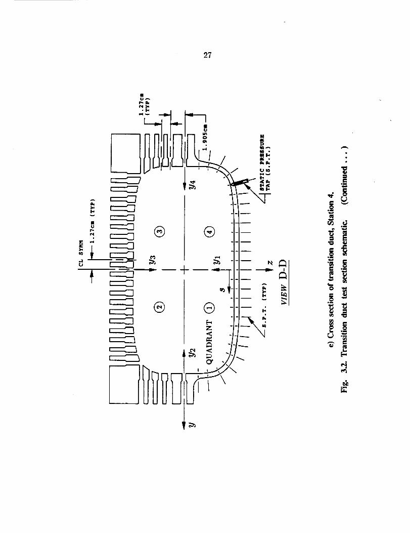
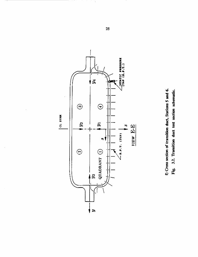
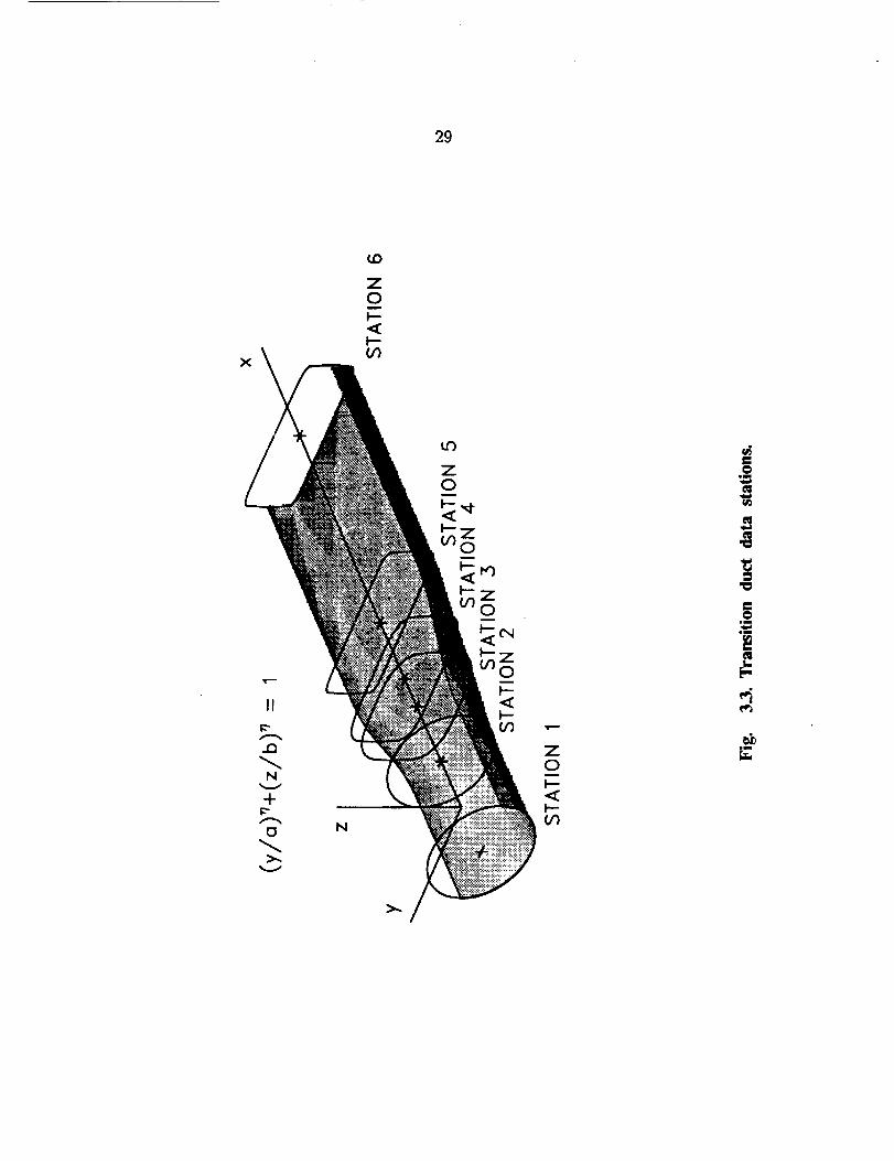
3.3 Test Section
A side view of the test section is shown in Fig. 3.2.a. Cross-sectional views
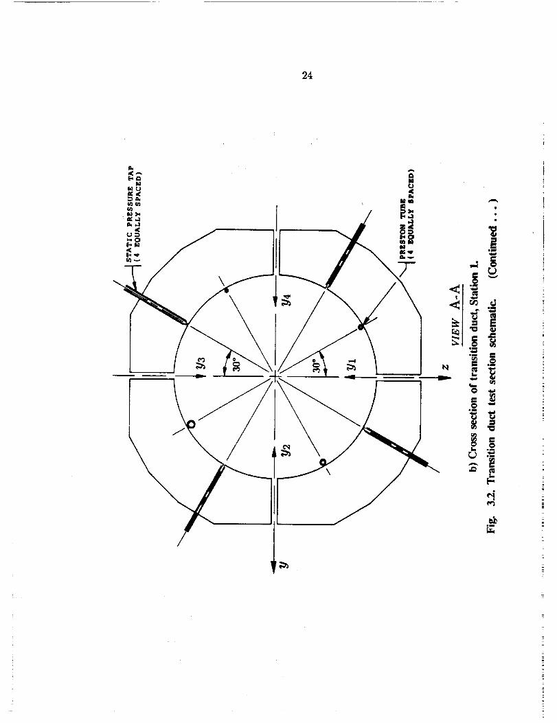
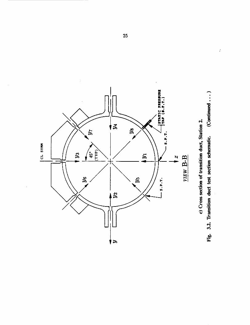
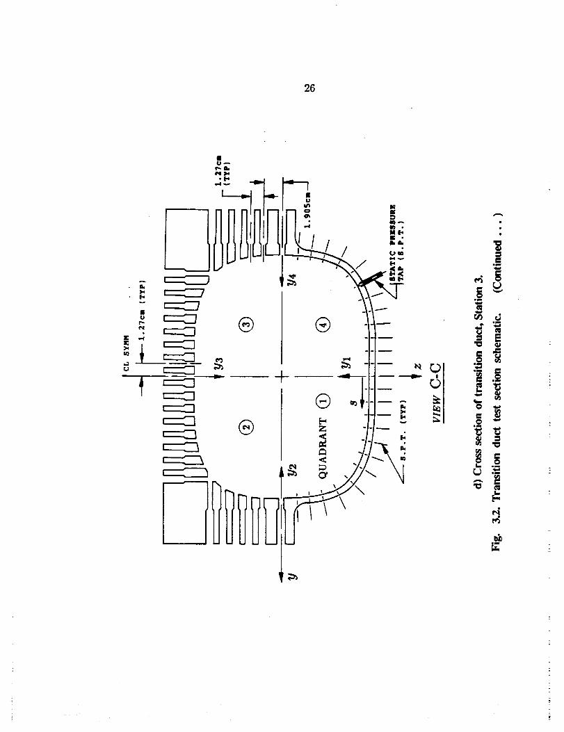
at each of the six data stations indicated in Fig. 3.2.a are shown in Figs. 3.2.b
through 3.2.f. The origin of the coordinate system shown in Fig. 3.2.a. was
chosen so as to be in agreement with NASA-Lewis' definition of the transition
duct. Station 1 is located one inlet duct diameter upstream from where the
beginning of transition occurs (Station 2). Although the cross section at Station
2 is still circular, it was anticipated that some distortion of the flow field will
occur due to the influence of the changing downstream geometry. At Stations 3
and 4 the geometry is changing rapidly and relatively large transverse velocities
were expected. Station 5 is located at the end of transition and data Station 6
is located two diameters downstream from the end of transition. An isometric
view of the six data station cross sections is shown in Fig. 3.3.
The probe traversing mechanism located just downstream of the test section
in Fig. 3.2.a was used for acquiring data at Stations 5 and 6. This mechanism
holds the probe axis parallel to the duct centerline and has provisions for rotating
the probe about it's longitudinal axis by means of a spring-loaded (anti-backlash)
bevel gear arrangement. Dial indicators were used to position the probes in each
direction to within an estimated accuracy of 4-0.025 ram, and the probes were
rotated to fixed angular positions to within an estimated accuracy of +0.5 degree.
The vertical and horizontal traversing capabilities are such that the probe can
be positioned anywhere within the cross section at Stations 5 and 6. However,
due to the convergence of the upper and lower walls of the transition duct, there
is an increasingly larger area upstream from Station 5 which cannot be accessed.
Therefore, at Stations 1 through 4 probes were inserted through holes in the
duct wall which are normal to the duct axial centerline. These access holes are
illustrated in Figs. 3.2.b through 3.2.e.
17
For this study, two identical transition ducts were constructed. The first of
these was used when taking data at Stations 1, 5 and 6. This duct has only static
pressure taps along the periphery of the lower half of the duct at Station 5 (see
Fig. 3.2.f). The second duct has probe access holes along the periphery of the
upper half of the duct and static pressure taps along the periphery of the lower
half of the duct at Stations 2, 3 and 4 (see Figs. 3.2.c through 3.2.e). Two ducts
were constructed to insure that there would be no influence on the flow field at
Stations 5 and 6 from probe access holes at upstream stations.
3.4 Instrumentation
The test section is instrumented to facilitate measurement of both mean
and fluctuating quantities. Mean quantities were measured by means of static
and total pressure instrumentation and hot-wire anemometry. All fluctuating
quantities were measured using hot-wire anemometry. Local skin friction was
measured with Preston tubes, which are simply circular Pitot tubes resting on
the duct wall.
A variety of pressure probes were used to measure the various mean quanti-
ties of interest. Total pressure contours were measured with two types of probes.
At Stations 1,2,5 and 6, where streamlines in the cross section are everywhere
nominally parallel to the axial center_ne of the duct, circular Pitot tubes having
an outside tip diameter of 0.635 mm were used. At intermediate data Stations
3 and 4, where the streamlines were skewed by as much as 20 degrees relative
to the probe centerline, a United Sensor Model KAC12 Kiel probe was used.
According to Chue [41], Kiel probes are able to measure total pressure accu-
rately for skew angles as high as 40 ° . Boundary layer profiles were measured by
means of flattened Pitot tubes having outer dimensions of 0.812 x 0.406 mm at
the tip. Static pressure distributions on the duct axial centerline were measured
by means of a static pressure probe which was traversed along the centerline.
Transverse flow angles were measured by means of a two-tube Conrad probe and
a normal hot-wire. All pressure data were measured with a 10 torr Barocel elec-
tronic manometer, Model 571D-10T-1C2-V1, coupled with a Datametrics digital
display unit, Model 1174.
Hot-wire probes consisted of single, rotatable normal and slant-wires. The
sensing element of the hot-wire probes is 0.00381 mm (4p) diameter platinum
coated tungsten wire. The ends of the wire are copper plated to facilitate sol-
dering and to define the sensing element length, which typically has a length-to-
diameter ratio near 300. The prongs of the probes are similar to configurations
recommended by Comte- Bellot et al. [42], for minimizing aerodynamic dis-
turbances. The fluctuating turbulence signal was processed by means of a TSI
Intelligent Flow Analyzer (IFA) system, which consists of an IFA 100 constant
temperature anemometer and an IFA 200 analog-to-digital (A/D) converter. The
18
digitized signal is recorded on a VAX Workstation, via a DRQ3B DMA card,
where the various turbulence correlations are computed. Appendix B contains a
description of the setup and operation of this equipment.
The probe access ring (see Fig. 3.2.a) was used to measure the flow conditions
at the transition duct inlet (Station 1). The ring contains four probe access
holes, four static pressure taps and four Preston tubes equally spaced around the
periphery of the ring as shown in Fig. 3.2.b. To ensure that Preston tube data
were taken within the law-of-the-wall region of the boundary layer, each Preston
tube was of a different diameter; 2.769, 3.962, 5.537 and 6.350 ram. The tubes
were semi-permanently installed and were removed before data were taken at the
downstream stations.
3.5 Data Reduction
This section contains the data reduction methods for the pressure probes,
hot-wire probes and equations for computing boundary layer parameters.
3.5.1 Pressure Probe Data Reduction
3.5.1.1 Mean Velocity
The total mean velocity along a flow streamline can be deduced from a
Pitot probe aligned with the streamline or, if alignment is not practical, from
measurements with a Kiel probe. The total velocity is related to the probe
pressure by Bernoulli's relation and the ideal gas law, namely:
Uo= 1/2 (3.1)
where:
by:
Uoh
Rair
To ., b
Pa ,,, b
= total velocity (re�s)
= measured pressure head (P, - P) (mmHo)
= gas constant for air (287.0J/(kg. *K))
= ambient temperature (°K)
= ambient static pressure (mmHg)
The Cartesian velocity components are related to the total velocity vector
U = U0cos/3cos3'
V = U0 sin/3 cos 7 (3.2)
W = U0 cos 13sin 7
where/3 and 7 are the flow angles in the x-y and x-z planes, respectively. These
flow angles can be measured directly by performing a differential pressure hulling
19
technique with a two-tube Conrad probe, first in the x-y plane and then in the
x-z plane.
3.5.1.2 Skin Friction
Head and Vasanta Ram's [43] tabulated presentation of Patel's [44] Preston
tube calibration was used to deduce local skin friction values. Their table presents
the calibration in the functional form:
A_.ppr_= f(-_2) (3.3)
where Ap is the difference between the Preston tube and local wall static pressureand d is the Preston tube outside diameter. Head and Vasanta Ram estimate
that, even without interpolation, their tables should give values that are accurate
to within 4-1 per cent. For the present study, a linear interpolation was used.
This method of evaluating shear stress presumes that the two-dimensional form
of the law-of-the-wall is valid and that streamwise pressure gradients are small.
It was anticipated that this method would be applicable to data taken at Stations
1,5 and 6, inasmuch as there is no longitudinal wall curvature or cross-sectional
area change at these locations.
3.5.2 Hot-Wire Probe Data Reduction
For reasons given in section 3.3, the positioning of the hot-wire probe is
dependent upon the particular station being investigated. At Stations 1 through
4, the probe body centerline was positioned in a direction normal to the axial
centerline of the duct, while at Stations 5 and 6 the probe was positioned parallel
to the axial direction. To simplify the following discussion, the former positioning
method shall hereafter be designated Method A, while the latter will be referredto as Method B
For the hot-wire measurements, single-wire techniques will be employed
rather than the more complicated two or three-wire methods. This approach
eliminates some of the difficulties associated with multi-wire techniques, such
as extensive calibration requirements, possible wire interference, multi-wire drift
and poor spatial resolution. Single-wire techniques, however, limit turbulence
measurements to second-order correlations (Reynolds stresses).
For Method B, a hot-wire technique developed by AI-Beirutty [45,46] and
Arterberry [47] was used to relate the three mean velocity components and six
Reynolds stresses to the mean and mean-square anemometer output voltages.
This technique uses a fixed normal-wire and a single, rotatable slant-wire and
utilizes an empirical cooling velocity law. The method is applicable to flows of
low-to-moderate turbulence intensity and zero-to-moderate flow skewness (up to
30 degrees total skewness in both pitch and yaw). Validation of the technique
20
for low-intensity turbulent flows was accomplished by analyzing data obtained
in fully-developed pipe flow under simulated skewed flow conditions [47]. For
moderate-intensity turbulent flows, validation was accomplished by obtaining
data under simulated skewed flow conditions in a free jet which issued from
fully-developed pipe flow [45]. The working forms of the mean and turbulence
response equations developed by A1-Beirutty are presented in Appendix C with-
out derivation. For details of the development of these equations, the reader is
referred to Refs. 45 and 46.
For Method A, appropriate hot-wire response equations are developed fol-
lowing a methodology similar to that used by A1-Beirutty. The working forms
of the response equations will be presented in Appendix C, with the details of
their derivation included in Appendices D and E. Also, following A1-Beirutty,
the Method A technique was partially validated in the present study by means
of data obtained in fully-developed pipe flow under simulated skewed flow con-
ditions. The verification procedure is described in Appendix F.
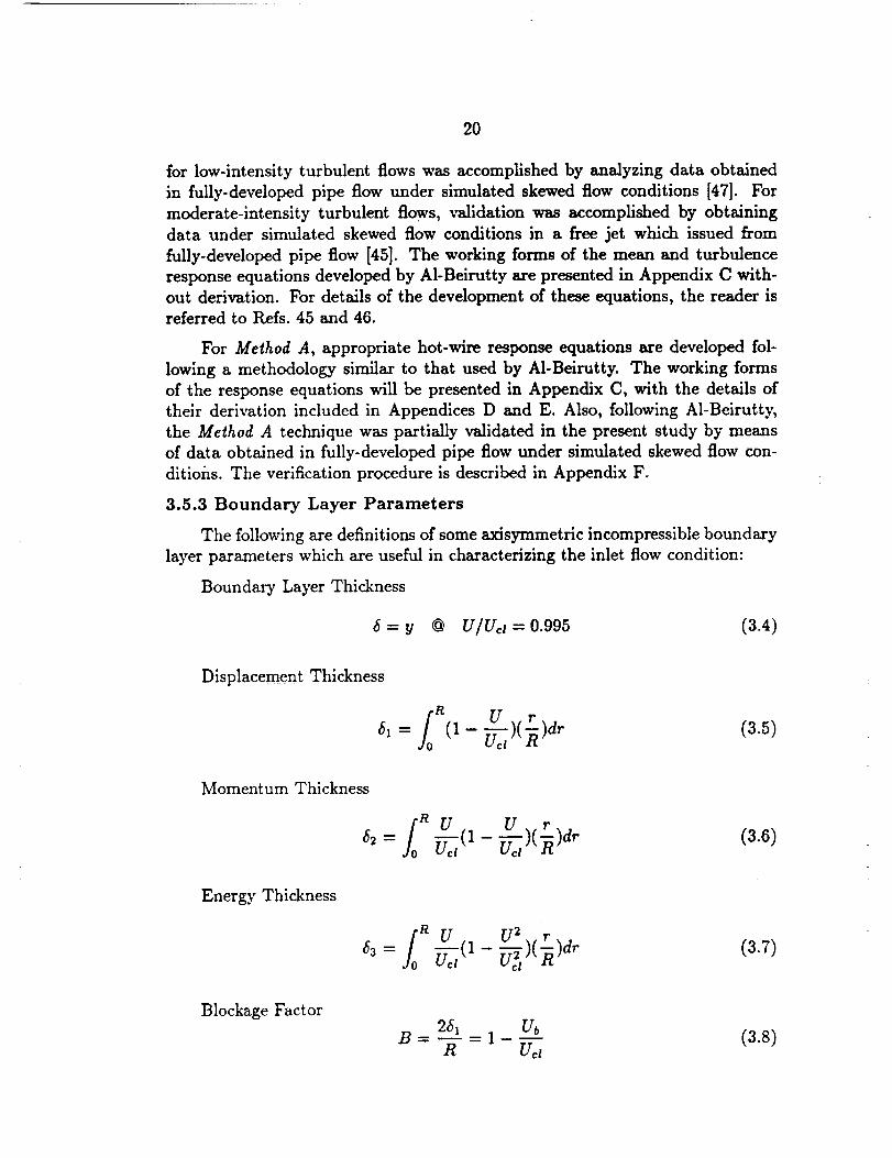
3.5.3 Boundary Layer Parameters
The following are definitions of some axisymmetric incompressible boundary
layer parameters which are useful in characterizing the inlet flow condition:
Boundary Layer Thickness
6=y @ U/Uc_=0.995 (3.4)
Displacement Thickness
fo n U r= (3.5)
Momentum Thickness
o n U U r
Energy Thickness
fo R U U 2 r
(3.6)
(3.7)
Blockage Factor25a U_
B- --1R UCt
(3.s)
21
First Shape Factor
H12 =/_-_ (3.9)
Second Shape Factor_3
H32 - _ (3.10)
It should be pointed out here that equations (3.5), (3.6) and (3.7) are approx-
imate, but that equation (3.8) is exact when the displacement thickness/_1 is
calculated by equation (3.5).
c_ >.,
0
_J(J
¢1
Z
,IF
c_
c_
o
c
:>.J
22
r
0
0
dlm
w
_m
_4
23
L
®
QQE)®
Q fmo_.J.r4
_o
f_
f-r-i k---_ _l---i _ --t_
/_ _"1]tF_1i!3_I1==- ll_z_,
_ L,J'_ '< ,-o
E
i"'_'1_ 0lilt I ,,,-i 0
-,,4
,, _N
--3a _a elu _
t_M01,)
24
\
25
El-INi#l
,.1
I
.m-p. ._
0 ,i
0Lm ill
gllr_
,A. l=
26
U
_ _=_
c_
U_
N_
®
®
\
27
28
29
(.0
II
N
÷
_ N

CHAPTER 4
INLET CONDITIONS
(Developing Pipe Flow)
4.1 Introduction :
The flow condition at Station 1 corresponds to partially developed turbu-
lent pipe flow. This seemingly simple flow case has been the subject of numerousexperimental and theoretical studies. Probably the most outstmading feature of
the work which has been done to date is the general lack of agreement among
the results of the various experimental investigations. Klein [48], after review-
ing more than a dozen turbulent developing pipe flow experiments, attributed
the disparities to the extreme sensitivity of upstream flow conditions on flow
development. Contraction ratio, boundary layer tripping devices and starting
conditions (smooth contraction vs. annular bleed) all influence local flow devel-
opment downstream of the pipe inlet. In addition, the use of a boundary layer
trip makes specification of the virtual origin of the boundary layer difficult.
Of the experimental studies, those due to Barbin & Jones [49], Richman
& Azad [50] and Reichert & Azad [51] are the most complete. The facility
used by Barbin & Jones incorporated a 4:1 circular contraction with an annular
bleed. A 2.54 cm wide strip of sand particles placed 5.1 cm downstream from the
leading edge of the pipe served as a boundary layer trip. The coordinate origin
was coincident with the leading edge of the pipe. Mean flow and turbulence
data were accumulated over a development length of 40 diameters for a bulk
Reynolds number of 388,000. In contrast, the facility used by Richman & Azad
utilized a smooth 89:1 circular contraction connected directly to the pipe. The
boundary layer was tripped with a 9 cm wide strip of # 16 sandpaper located
at the entrance to the pipe. The coordinate origin was chosen to coincide with
the downstream edge of the boundary layer trip, although the authors estimate
the virtual origin of the boundary layer to be 3 cm upstream of this location.
Data for this study were collected over a development length of 70 diameters
for bulk Reynolds numbers of 100,000, 200,000 and 300,000. Reichert & Azad
used the same facility as Richman & Azad but report that a 5.1 cm wide strip of
unspecified sandpaper was used as a trip. Data for this study were collected over
a development length of 70 diameters for seven bulk Reynolds numbers between
112,000 and 306,000.
The experimental data of Barbin & Jones and Richman & Azad were recently
used by Martinuzzi £: Pollard [52,53] for comparative purposes in a comprehen-
sive evaluation of 11 turbulence models: 4 algebraic models, 2 k-e models and
5 Reynolds stress models. All models were implemented in the same computer
PJ_ ._0 I_TENTIONALLY BLA,_KPRECEDING PAGE BLANK NOT FILMED
32
code using equivalent boundary conditions. Although each model had its own
merits and drawbacks, the low Reynolds number form of the k-e model overall
performed best.
4.2 Preliminary Results
Preliminary measurements were made at Station 1. The purpose of these
preliminary measurements was: 1) to establish the range of operating Reynolds
number attainable and 2) to determine the lowest operating Reynolds number
where fully turbulent flow exists at the first data station. The results of these
measurements follow.
The wind tunnel was initially configured with three inlet pipes (L/D =
9) and the boundary layer was allowed to develop naturally within the pipe,
i.e. no boundary layer trip was present upstream. Pitot tube surveys of the
bouri.dary layer at Station 1 were obtained for two arbitrary Reynolds numbers,
Reb = 234,000 and 403,000, the latter Reynolds number being very near the
upper operating limit of the wind tunnel. Assuming constant static pressure
across the data plane, mean velocity profiles were computed by equation (3.1).
These results were plotted in law-of-the-wall coordinates using friction velocities
deduced from measurements with the four different diameter Preston tubes shown
in Fig. 3.2.b. Agreement with the theoretical law-of-the-wall profile was found to
be poor, indicating that the boundarY layer was not yet in a fully turbulent state.
To promote transition to turbulence, a 2.54 cm wide strip of # 36 grit sandpaper
was applied around the periphery of the first inlet pipe, 1.27 cm downstream
from the joint, as shown in Fig. 3.1. With the boundary layer trip in place the
pitot tube surveys were repeated at nominally the same Reynolds numbers. A
comparison of mean velocity profiles with and without the boundary layer trip
at the two Reynolds numbers is shown in laboratory coordinates in Fig. 4.1.a.
and in law-of-the-wall coordinates in Fig. 4.1.b. These results indicate that the
sandpaper trip was effective in producing a fully-turbulent boundary layer at the
inlet station.
4.3 Range of Operating Conditions
With the boundary layer trip installed, the range of operating Reynolds
number was found to be 0 <Rect < 479,000 (0 < Reb <_ 442,000). The
presence of the boundary layer trip, however, does not guarantee a turbulent
boundary layer over the entire operating Reynolds number range, indeed, the
Preston tube calibration is valid only when law-of-the-wall behavior is present.
Since the Preston tubes had to be removed before taking data at downstream
stations, and the operating Reynolds numbers for data acquisition had as yet not
been established, a correlation between friction velocity and centerline Reynolds
number was obtained. This allows the inlet skin friction condition to be known
for any operating Reynolds number, provided that the flow is fully turbulent.
33
This correlation for the four Preston tubes is shown in Fig. 4.2. Agreement isgenerally good for the different diameter tubes, with the exception of resultsreferred to the largest tube at centerline Reynoldsnumbersabove425,000.Thereasonfor this deviation is that the boundary layer thins asthe Reynoldsnumberis increased, allowing the largest tube to extend beyond the law-of-the-wall region
where the Preston tube calibration is valid. Another small deviation, which was
repeatable, occurs in: the neighborhood of Rect=220,000. The cause for this is
unknown, but may be associated with an unsteadiness in the wind tunnel at that
operating condition. Also indicated in Fig. 4.2 is the approximate region where
fully turbulent flow begins. The determination of this region will be discussed
shortly. Using the points outside the transition region, an empirical correlation
was determined that describes friction velocity behavior at Station 1:
U, = 0.255 - 0.0712 log 10( Re ct) + 0.00577 log_ 0 (Rect)Uct
(4.1)
which is applicable in the range 97,000 < Rect< 460,000.
A simple indication of fully turbulent flow is whether or not law- of-the-wall
behavior is observed within the boundary layer. Fig. 4.1 shows that law-of-the-
wall behavior exists at Red = 255,000 (Reb = 234,000). To estimate the lower
limit of fully turbulent flow, Pitot profiles were measured at two relatively low
Reynolds numbers, Rect = 55,000 and 97,000 (Reb = 52,000 and 88,000). These
results are plotted in laboratory coordinates in Fig. 4.3.a and in law-of-the-wall
coordinates in Fig. 4.3.b. The mean profile at the lower Reynolds number is
considerably thinner than the higher Reynolds number profile and appears to
have a laminar-like shape. In addition, this profile clearly does not follow law-
of-the-wall behavior. An examination of the boundary layer shape factor, H12,
indicates, however, that the flow is not fully laminar either. For the present
profile a shape factor of H12 = 2.0 was measured, whereas typical values for
the fully laminar and fully turbulent profiles are 2.6 and 1.4, respectively [48].
Conversely, the higher Reynolds number profile corresponds to a thick boundary
layer that agrees well with the law-of-the-wall and has a measured shape factorof 1.4.
Based on the above results, it was decided that data for the turbulent flow
case would be taken at bulk Reynolds numbers of 88,000 and 390,000, for which
the inlet flow at data Station 1 (refer to Fig. 3.2.a) should be fully turbulent.
The upper value represents the maximum operating speed of the wind tunnel
throttled back slightly to allow adjustment for variations in ambient conditions.
4.4 Results and Discussion
For the present study, data were collected at a development length xp/D
= 9, where xp = 0 corresponds to the pipe inlet. It is likely that the effective
34
length is slightly larger, inasmuch as a boundary layer is already developingin the contraction and the sandpaper trip tends to thicken the boundary layer
artificially. The transverse flow angle in the azimuthal direction was measured
using a pressure-hulling technique with a two-tube Conrad probe. The probe was
first nuUed at the pipe centerline and then the flow angle along the t/1 traverse (see
Fig. 3.2.b) was measured relative to the centerline null value. For both operating
Reynglds numbers, the computed transverse flow velocity (Us) was found to be
less than 0.25% of the local axial velocity component across the entire traverse.
Mean velocity profiles plotted in laboratory coordinates and in law-of-the-
wall coordinates along four equally-spaced radial traverses at Station 1 are shown
for Reb = 88,000 and 390,000 in Figs. 4.4 and 4.5, respectively. The excellent
peripheral symmetry of the flow and agreement with law-of-the-wall behavior
are readily apparent. The non-dimensional Preston tube diameters (d +) used
to deduce skin friction are indicated on the law-of-the-wall plot. The largest
tube for the higher Reynolds number case extends slightly into the wake region
and, as a result, skin friction values deduced from this tube were slightly higher
than those for the three smallest tubes. Friction velocities deduced from the three
smallest tubes deviated by less than 0.3% from their mean value. Boundary layer
thickness, integral parameters, skin friction and centerline turbulence intensity
at Station 1 are summarized in Table 4.1. The integral parameters shown are
averages of values computed from the four individual traverses.
Table 4.!. Flow condition at Station 1
Reb = 88,000 Reb = 390,000
g/R 0.3141 0.2855
61/R 0.0448 0:0383
62/R 0.0312 0.0281
_3/R 0.0545 0.0497B 0.0896 0.0765
H12 1.438 1.364
H32 1.748 1.771
Tw/7"w,fD 1.00 0.96
(u'/U)cl 0.008 0.003
R = 10.214 cm
As expected, the boundary layer is somewhat thicker for the lower Reynolds
number case. The H12 shape factors agree well with those reported by Klein
for fully turbulent, developing pipe flow. The wall shear stress in Table 4.1. has
been normalized by the fully-developed pipe flow shear stress _',,,,FD which was
determined from a relation given by Eppich [40]. Data presented by Reichert
_z Azad show that when a smooth contraction is used as the starting condition,
35
the skin friction at the entrance to the pipe is below the fully-developed value
and that the skin friction approaches the fully-developed value in an oscillatory
manner. In contrast, Barbin & Jones data show that when a sharp edge is used
as a starting condition, the skin friction at the beginning of the pipe is above the
fully-developed value but asymptotically reaches the fully-developed value within
the first 15 diameters. The present results show that the wall shear stress at xp]D
= 9 is very near the fully-developed value. At the lower Reynolds number, the
flow was much more susceptible to ambient disturbances and this is reflected in
the larger data scatter and higher freestream turbulence levels.
Reynolds normal and shear stress distributions at Station 1 for Reb = 88,000
and 390,000 are shown in Fig. 4.6. Experimental results obtained by Barbin &
Jones and Richman & Azad at a comparable location (zv/D = 10) and operating
Reynolds numbers are also shown for purposes of comparison. The turbulence
levels shown in these plots near the pipe centerline should not be considered
representative of the core flow turbulence intensity, inasmuch as the output from
the probe used to measure the distributions exhibited a small sinusoidal trace on
the oscilloscope when positioned in the core flow. This noise was attributed to
vortex shedding from the probe prongs when the probe was positioned normal
to the axial mean flow. The turbulence intensity values shown in Table 4.1. are
correct and were measured independently using a forward-facing probe fixed at
the duct centerline.
The Reynolds stress profiles in Fig. 4.6 are seen to be nearly Reynolds num-
ber independent over the range considered. Based on the turbulence results, it
appears that the boundary layer in the present study is thinner than that of the
other investigators. In the near-wall region, the normal stresses are seen to be
significantly higher than those due to Barbin & Jones. The shear stress in the
near-wall region agrees well with the results of Richman & Azad and with the
fully-developed distribution.
The more rapid boundary layer growth associated with Richman and Azad's
experiments can probably be attributed to the rougher and wider sandpaper
tripping device used in their study, which extended over a streamwise width of
0.9 pipe diameters in comparison to the width used in the present study (0.12
pipe diameters). In Barbin & Jones' experiments, a sand grain trip of the same
relative width as that used in the present study was employed. By-pass bleed
through an annular gap between the pipe and a 4:1 contraction ratio nozzle was
used to promote spanwise flow uniformity across the pipe inlet. In reference to
Fig. 1 of Ref. 49, the pipe in Barbin & Jones' experiments extended upstream
into the nozzle, so that the pipe inlet could have been in a region where the flow
was still converging, and the flow may have separated at the wedge-shaped lip of
the pipe. This event, if it occurred, could have promoted more rapid boundary
layer growth in comparison to that observed in the present study. If local flow
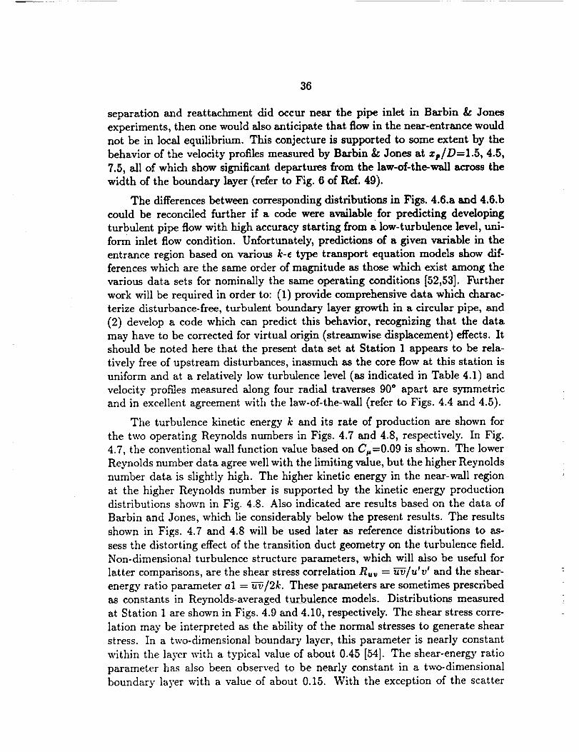
36
separation and reattachment did occur near the pipe inlet in Barbin & Jones
experiments, then one would also anticipate that flow in the near-entrance would
not be in local equilibrium. This conjecture is supported to some extent by the
behavior of the velocity profiles measured by Barbin & Jones at zp/D-1.5, 4.5,
7.5, all of which show significant departures from the law-of-the-wall across the
width of the boundary layer (refer to Fig. 6 of Ref. 49).
The differences between corresponding distributions in Figs. 4.6.a and 4.6.b
could be reconciled further if a code were available for predicting developing
turbulent pipe flow with high accuracy starting from a low-turbulence level, uni-
form inlet flow condition. Unfortunately, predictions of a given variable in the
entrance region based on various k-e type transport equation models show dif-
ferences which are the same order of magnitude as those which exist among the
various data sets for nominally the same operating conditions [52,53]. Further
work will be required in order to: (1) provide comprehensive data which charac-
terize disturbance-free, turbulent boundary layer growth in a circular pipe, and
(2) develop a code which can predict this behavior, recognizing that the data
may have to be corrected for virtual origin (streamwise displacement) effects. It
should be noted here that the present data set at Station 1 appears to be rela-
tively free of upstream disturbances, inasmuch as the core flow at this station is
uniform and at a relatively low turbulence level (as indicated in Table 4.1) and
velocity profiles measured along four radial traverses 90 ° apart are symmetric
and in excellent agreement with the law-of-the-wall (refer to Figs. 4.4 and 4.5).
The turbulence kinetic energy k and its rate of production are shown for
the two operating Reynolds numbers in Figs. 4.7 and 4.8, respectively. In Fig.
4.7, the conventional wall function value based on C_,=0.09 is shown. The lower
Reynolds number data agree well with the limiting value, but the higher Reynolds
number data is slightly high. The higher kinetic energy in the near-wall region
at the higher Reynolds number is supported by the kinetic energy production
distributions shown in Fig. 4.8. Also indicated are results based on the data of
Barbin and Jones, which lie considerably below the present results. The results
shown in Figs. 4.7 and 4.8 will be used later as reference distributions to as-
sess the distorting effect of the transition duct geometry on the turbulence field.
Non-dimensional turbulence structure parameters, which will also be useful for
latter comparisons, are the shear stress correlation Ruv = "ff'_/u'v' and the shear-
energy ratio parameter al = _-_/2k. These parameters are sometimes prescribed
as constants in Reynolds-averaged turbulence models. Distributions measured
at Station 1 are shown in Figs. 4.9 and 4.10, respectively. The shear stress corre-
lation may be interpreted as the ability of the normal stresses to generate shear
stress. In a two-dimensional boundary layer, this parameter is nearly constant
within the layer with a typical value of about 0.45 [54]. The shear-energy ratio
parameter has also been observed to be nearly constant in a two-dimensional
boundary layer with a value of about 0.15. With the exception of the scatter
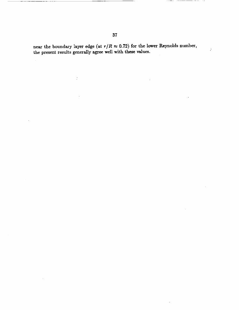
37
near the boundary layer edge (at r/R _, 0.72) for the lower Reynolds number,
the present results generally agree well with these values.
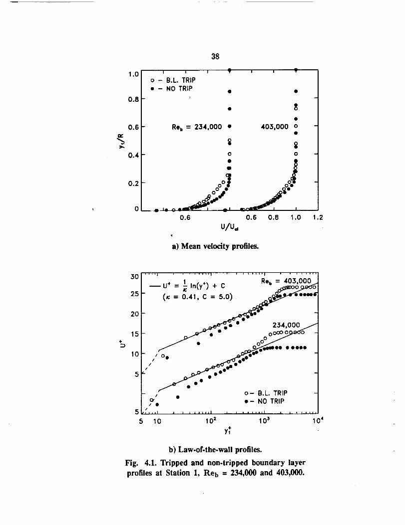
38
I ' ' ' _ ' ' ; I1"°I o - BL Trap I
L . - NO TRIP • • _0.8
/ • :/o.+r ,.,=_,.ooo• ,o_.ooo: 10.4 o o
0.2
0
0.6 0.6 0.8 1.0 1.2
u/u_
a) Mean velocity profiles.
30 .... ' ..,' 'I '. '_ '+'_'_ ..' ...... R% = 403',000_
20-25- (_:= 0.41, C = 5_e=_
/ _ * " 234,000/
lsl- /. - oo_O -• oo_ L_" .__.o.......
;oI ,, o. _....-
s_- _0""
L , _'_r_ It- o- B.L. TRIP -
_e • e- NO TRIP5L_i ,+=| | I I = i ===I l , l , , J,,l _ l . J . ,._
5 10 10 = 103 104
yt
b) Law-of-the-wall profiles.
Fig. 4.1. Tripped and non-tripped boundary layer
profiles at Station 1, Reb = 234,000 and 403,000.
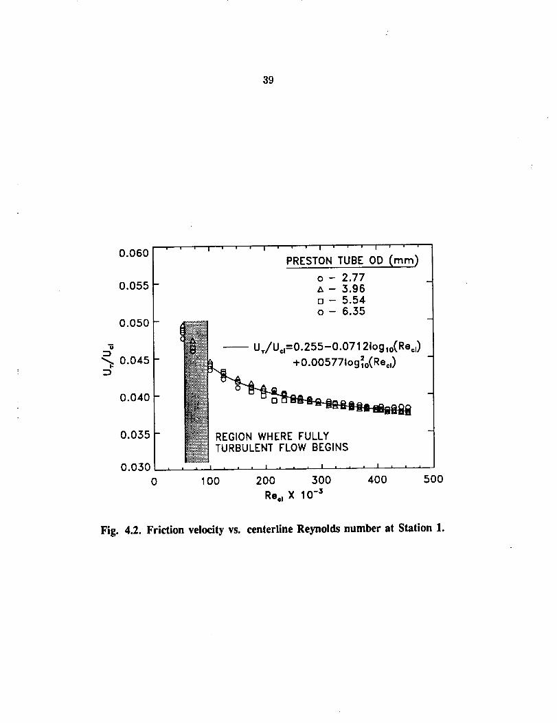
39
0.060
0.055
0.050
wO
:Z)o.o4s
0.040
0.035
' ' ' I ' ' ' I ' ' ' I ' ' ' I ' ' '
PRESTON TUBE OD (ram)
o - 2.77m
A- 3.96n- 5.54o- 6.35
._"_ .i
.... U,/U=,=0.255-O.07121Og,o(Re=, )
,= +O'O05771°g_o(Re©,):_i
_i::: m
Ii
ii ig -rL-ow-i G,NS
0.030 . . . _ . . , I , . . , . . . = . . .
0 1O0 200 300 400 500
Re,l X 10 -=
Fig. 4.2. Friction velocity vs. centerline Reynolds number at Station 1.
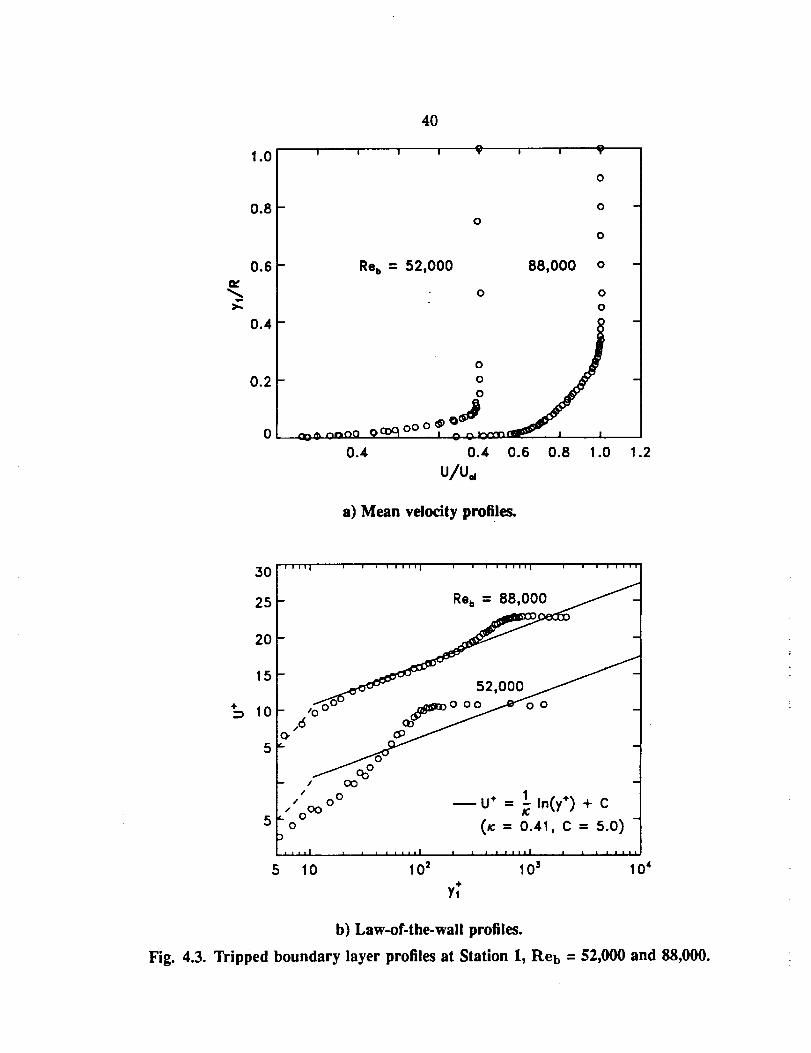
er
1.0
0.8
0.6
0.4
0.2
0
4O
I I I I (_ I I
0
9
0
0
0
Reb = 52,000 88,000 o
0 0
0
0
_ _¢_oo O_ _ _ _ _
0.4 0.4 0.8 o.8 1.ou/u,,
a) Mean velocity profiles.
.2
3O
25
20
15
lO
5
5
j ....i i i i i I _ i i i ii I i i i ! i i ii I i ! i i i i _;
,o_ 52,oo=ooo°_=_ "__"
- / O0
// 0 0
L" 000
0
i Jl*l l • [ i i =111
5 10 10 2
U+ = _I in(y+) + C
(Ic = 0.41, C = 5.0)
i i i i 111|1 • • • 1111
10 3
y_0 4
b) Law-of-the-wall profiles.
Fig. 4.3. Tripped boundary layer profiles at Station I, P,.eb = 52,000 and 88,000.
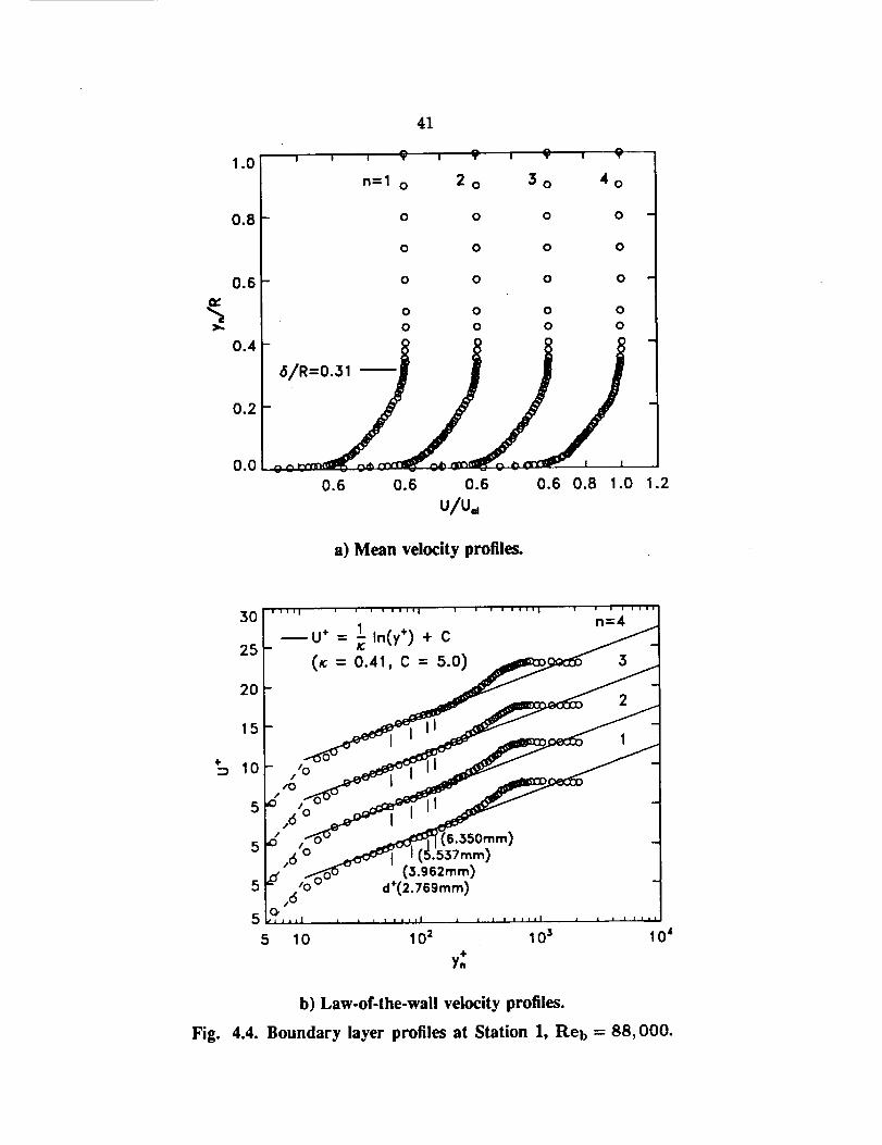
e,,
1.0
0.8
0.6
41
I I , 9
n=l o
, 9 , 9 , 9
20 30 40
0 0 0 0
0 0 0 0
0 0 0 0
0 0 0 0
0 0 0 0
0.4
" °
0.2
0.0
0.6 0.6 0.6 0.6 0.8 1.0 1.2
U/Ud
a) Mean velocity profiles.
30
25
20
15
5
5
5
5
5
i i i i i , i _ i i , i i i i i ! ! , i il I i i ! , , , .!
' 2 -
I I II 1 _.,
d+(2.769mm) ]_tt alll l I l i i = iii l I | i i ltli I I I i L I i
10 102 10s 10 't
b) Law.of-the-wall velocity profiles.
Fig. 4.4. Boundary layer profiles at Station I, Reb = 88,000.
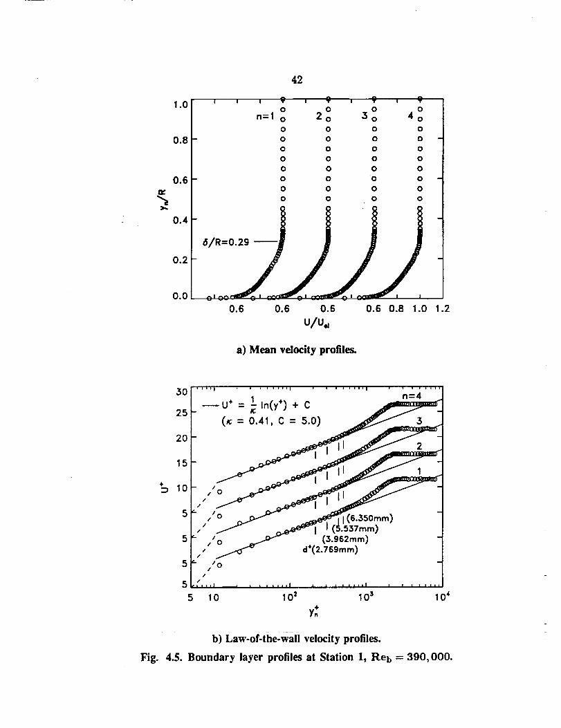
42
1.0 I , I 9 I 9 l "_ lO 0 0 0
n-| o 2o 3o 4o0 0 0 0
0.8- o o o o0 0 0 0
0 0 0 0
0 0 0 0
0.6- o o o o0 0 0 0
0 0 0 0
0.4
0.2
0.0
0.6 0.6 0.6 0.6 0.8 1.0 1.2
u/u,,
a) Mean velocity profiles.
Fig.
4-
30
25
20
15
10
5
5
5
5
5
I In(y,) + C_U+= _.
(pc = 0.41, C = 5.0)
//0
/
/
//0/
/
//0/
/
//0
/
/
'6.350mm)
537mm)(3.962mm)
d+(2.769mm)
n=4
3
2
1
10 102 103 10 4
y:
b) Law-of-the'wall velocity profiles.
4.5. Boundary layer profiles at Station 1, Reb = 390,000.
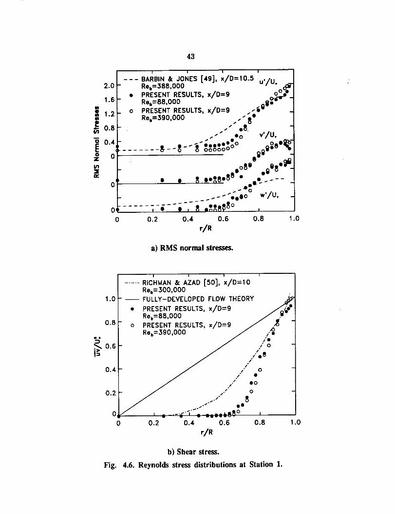
43
2.0
1.6
81.2
_l 0,8
o.41
_" Oq
O I
0
BARBIN &: JONES [49], x/D=IO.5' ,,. I- R%=388,000 u/u,
• ,i<>:,o PRESENT RESULTS, x/D=9 .'ll 4
R%=390,000 ,, ,,, " 8e J.. o8 .. G
." to v/U, /
_ -o'--g_:_o,:ooO _,o,,-,_Io8O el tt.ol Ilt]
.o ell o -I
• e Ill ion8 °8° " o"-0-- t..... _ - ""cello w'/U, -'l
;" , -_ - - ; , 8 ._I1_ tf° , /0.2 0.4 0.6 0.8 1.0
r/R
a) RMS normal stresses.
,,,,,
I I I I
..... RICHMAN .itAZAD [sol, x/D=lOR%=300,OOO
1.0 FULLY-DEVELOPED FLOW THEORY
• PRESENT RESULTS, x/D=9 //_'t"lJ_'l
R%=88,000 / m _]0.8 o PRESENT RESULTS, x/D=9 / _ i
R%=390,000 _ _'_o./'
0.6- /o -
0.4 - J /./" eo -
/ .°0.2 - / ,." 0 -
_.....i oo _O , ;--_", = =_==_=__o ,
O 0.2 0.4 0.6 0.8 1.0
r/R
b) Shear stress.
Fig. 4.6. Reynolds stress distributions at Station l.
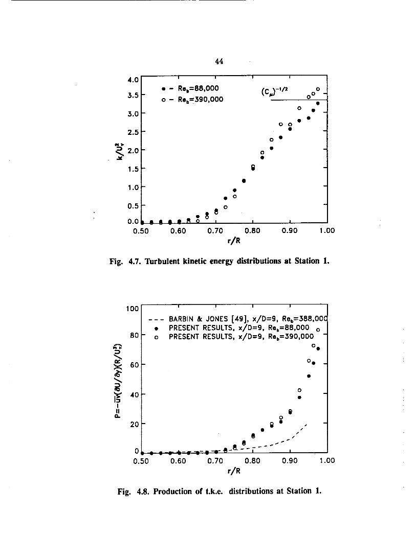
44
4.0
3.5
3.0
2.5
NI.
1.5 --
1.0-
0.5
0.0
0.50
I I
•- R%=88,000
o- R%=390,000
o
g
(C_ -_/= ° o° -
• 0
08
! !
0.70 0.80
0 • -
0 0•
0 •
•
m
•8, ,, a _ _ _ o
0.60 0.90 1.00
Fig. 4.7. Turbulent kinetic energy distributions at Station 1.
100 _
8O
_, 60
40
20
0,
0.50
o
I I I I
BARBIN &: JONES [49], x/D=9, R%=388,00CPRESENT RESULTS, x/D=9, Reb=88,000 oPRESENT RESULTS, x/D=9, Reb=390,O00 -
o I
o e _
_ o -
8 8
, _¢_¢_j.._¢. -.r,8-8---_ ---- ..-.- = _ I
0.60 0.70 0.80 0.90 1.00
r/R
Fig. 4.8. Production of t.k.e, distributions at Station 1.
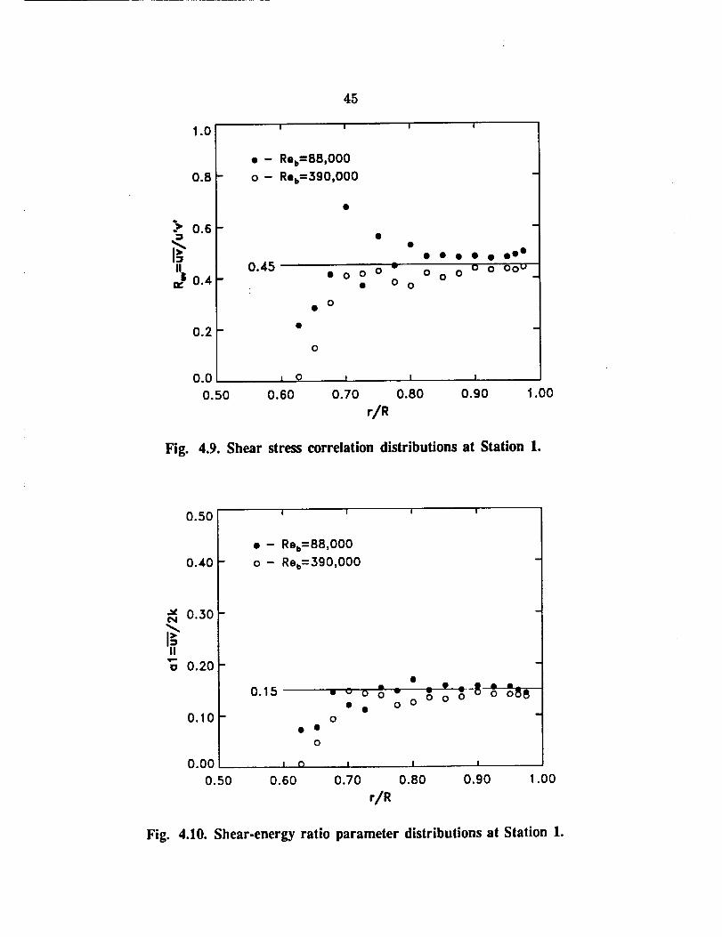
45
1.0
0.8
:> o.6-=1
IIB 0.45uc 0.4-
0.2-
0.0
0.50
I I I I
•- Rob=88,000
o- Ro1,=390,000
O0 oo
0
0000000 O
0000°000 U
0 o
i q t i i
0.60 0.70 0.80 0.90
r/R
.00
Fig. 4.9. Shear stress correlation distributions at Station 1.
0.50
0.40
.x 0.30¢'4
IIo 0.20
0.15
0.10 -
0.00
0.50
I I
•- Rob=88,000
o- R%=390,000
0 0 0 "
0
I I
oo_OOO_80 o
• •
0
I 0 I I I
0.60 0.70 0.80 0.90 1.00
Fig. 4.10. Shear-energy ratio parameter distributions at Station 1.

CHAPTER 5
RESULTS AND DISCUSSION
5.1 Introduction
The sequence in which data were collected in the transition duct is as follows.
The first transition duct was installed and the peripheral wall static pressuredistributions at each data station were obtained. Data were then accumulated at
Station 5 to check flow symmetry and determine the extent of Reynolds number
dependence of the flow. The transition duct extension was then installed and
data were accumulated at Station 6. Finally, the second transition duct was
installed and measurements were made at the intermediate Stations 3 and 4. No
data were taken at Station 2. Total pressure and mean velocity were deduced
from hot-wire measurements made at Stations 3,4,5 and 6. Turbulence quantities,
however, were only measured at Stations 5 and 6 since the anticipated vortex
structure was not well defined until Station 5.
At all stations, symmetry was assumed about the x-z plane and, as such,
data were accumulated only in Quadrants 1 and/or 2 shown in Figs. 3.2.d-3.2.f.
At Stations 3 and 4, due to the arrangement of the probe access holes (see Figs.
3.2.d and 3.2.e), data were taken only in Quadrant 2. For presentation purposes,
the data were imaged about the y-axis to show an entire duct half. All subsequent
plots where data have been imaged are so indicated. The spacing between data
points along individual traverses varied from 1.27 cm in the core region to 0.127
cm near the wall surface. At Stations 5 and 6, rather than assuming symmetry
about the midplane z=O, measurements were made in both Quadrants 1 and
2. Data were taken at selected points on a 63 x 19 rectangular grid (0.254 cm
spacing) in each quadrant. The spacing between data points varied from 2.54
cm in the core region to 0.254 cm in regions of large gradients. Approximately
400 data points were taken in the duct half. It should be emphasized here that
all subsequent contour results for Stations 5 and 6 are based on data obtained in
both quadrants, so that the level of symmetry about the x-y plane of the duct is
a direct indication of the quality of the flow and of the measurement techniques
employed in this study. For plotting purposes, the measured results at all stations
were interpolated onto an evenly spaced mesh by means of a monotonic derivative
spline interpolant [55]. This method of interpolation performs no smoothing and
guarantees no overshoot of the data.
5.2 Static Pressure Distribution
Wall static pressure distributions were measured along the periphery (s-
coordinate, refer to Figs. 3.2.d through 3.2.f) of the lower half of the duct at
P,,A__INTENTION_LLy BLANK PRECEDIb,'G PAGE BLANK NOT FILMED
48
Stations 3,4,5, and 6. Peripheral wall static pressure coefficient distributions are
shown for Reb = 88,000 and 390,000 in Fig. 5.1. The normalizing dimension 8re!
is 1/4 of the duct circumference at a given data station. Solid symbols represent
static pressure measured along the duct centerline. The excellent spanwise regu-
laxity at all stations supports the assumption of symmetry about the z-z plane.
The primary difference between results referred to the two Reynolds numbers
is that the net pressure coefficient drop along the duct is larger for the lower
Reynolds number case and is the result of increased viscous losses associated
with the more rapid boundary layer growth.
Local static pressure is a function of cross-sectional area, wall curvature
and viscous forces. Station 3 is located at an axial position where streamwise
diffusion of the flow is occurring. In reference to Fig. 5.1, this results in a net
rise in static pressure above the inlet value (Cp=O) which is reflected in the
centerline pressure. Concave curvature along the upper wall (s/s,.eI=O) induces
a positive pressure gradient (aP/Or > 0) which results in the observed pressure
peak. Conversely, convex wall curvature along the sidewalls (S/Sre¢=:i:l) induces
a negative pressure gradient resulting in the pressure minima. A net decrease
in static pressure occurs between Stations 3 and 4 which is the result of a slight
decrease in cross-sectional area and viscous losses. Also, the radius of curvature
of the walls changes sign between Stations 3 and 4 which causes maximum and
minimum pressures to occur along the side and upper walls, respectively. At
Station 5 the area has returned to the inlet value so that a net decrease in pressure
relative to the inlet occurs which is due only to viscous effects. Although there
is no curvature of the walls at this station, upstream curvature effects (the wall
curvature peaks between Station 4 and 5) are still strongly present. At Station 6,
there is no area change or curvature effects, and the static pressure is nominally
constant across the entire cross section.
5.3 Effect of Varying ReynOlds Number
Results presented thus far have shown that, aside from a thicker boundary
layer at the lower operating Reynolds number, no appreciable Reynolds num-
ber dependence exists over the limited range considered. In order to determine
the influence of Reynolds number on downstream flow development, mean flow
measurements and some limited turbulence data were accumulated at Station
5 for operating bulk Reynolds numbers of 88,000 and 390,000. Total pressure
contours, axial mean velocity contours and transverse velocity vectors for the
two operating conditions are shown in Figs. 5.2, 5.3 and 5.4, respectively. These
results are shown here only for comparison; the physical significance of the flow-
field behavior will be discussed in the next section. In Fig. 5.4, the reference
velocity vector represents the largest measured vector in the plane. The mean
flowfields at the two operating conditions are observed to be very similar. One
notable difference is that the vortex pair for the lower Reynolds number is more

49
circular and centered further away from the wall. Overall, though, the differences
observed were not significant enough to justify repeating all measurements for
both operating conditions. It was decided, therefore, to restrict the bulk of the
measurements at the remaining stations to one operating condition. Since, for
most practical applications, the operating condition for a circular-to-rectangular
transition duct would be closer to the higher operating condition, most of the
remaining measurements axe for the Res = 390,000 case.
$.4 Mean Flow Results
5.4.1 Mean flow contours
Mean flow variables were measured in the transverse plane at Stations 3,4,5
and 6. Reference coordinates applicable to theses data stations are shown in
Figs. 3.2.d through 3.2.f, respectively. Total pressure contours (Pitot probe)
and axial velocity contours (hot-wire probes) at Stations 3,4,5 and 6 are shown
in Figs. 5.5 and 5.6, respectively. At Station 3, the total pressure and axial
velocity contours generally follow the cross- sectional shape of the duct. At
Station 4, a distortion of the contours is seen to develop in the vicinity of the
sidewall. The data at Stations 5 and 6 show that the distortion grows in the axial
direction. The development of the distortion is qualitatively very similar to the
results presented by Taylor et al. [39] for turbulent flow through a non-diffusing
S-shaped duct. Transverse velocity vectors measured by means of hot-wires are
shown in Fig. 5.7. The magnitude of the reference velocity vector indicated in the
plots represents the maximum vector magnitude observed at that station. The
distortion of the primary flow is due to a secondary flow pattern which develops
into a discrete vortex pair along the duct sidewalls. This secondary flow arises
as a result of lateral skewing of the near-wall flow in the vicinity of the sidewall
induced by transverse pressure gradients (refer to Fig. 5.1) associated with wall
curvature. At Station 5, the vortices are oblong in shape and their centers are
positioned relatively near the duct sidewall. At Station 6, the vortices have
grown in lateral extent, are more circular and are centered further away from the
sidewall. Between Stations 2 and 5, lateral divergence of the upper (lower) wall
boundary layer and lateral convergence of the sidewall boundary layer causes
thinning and thickening of the boundary layer, respectively. Between Stations
5 and 6, the boundary layer everywhere thickens by natural growth and, in the
vicinity of the sidewall, by lateral convergence.
The static pressure distribution at Station 5 was measured directly with a
static pressure probe and calculated from the total pressure and velocity distri-butions:
1 2P- P, - _Pa,,_bU_/(R,_i,T,,mb) (5.1)
where the variables are defined as in equation (3.1). Measurement of the static
pressure at Station 5 was possible since the total flow angle is less than 10 °.
5O
The measured and calculated distributions are shown in Fig. 5.8. The measured
static pressure in the near wall region agrees well with the wall tap measurements
shown in Fig. 5.1.b. The calculated pressure field qualitatively agrees with the
measurements, but doesn't show the saddle-shaped distributions as clearly.
5.4.2 Boundary layer divergence
The mean velocity distributions were used to estimate the strength of the
divergence along the midplanes y=0 and z=0 (negative divergence is the same
as convergence). On the midplane y=0 (upper wall), the divergence parame-
ter is defined as (OV/Oy)/(OU/Oyl) evaluated midway through the boundary
layer. On the midplane z=0 (side wall), the divergence parameter is defined as
(OW/Oz)/(OU/Oy2) evaluated at the first data point from the wall (_ 0.5 cm).
An estimate of the axial distribution of these divergence parameters is shown in
Fig. 5.9. Along the duct upper (lower) surface, the divergence is, for the most
part,:conflned to the actual transition section, peaking at around 20%. To fur-
ther illustrate the degree of divergence on the upper and lower surfaces of the
duct, Fig. 5.10 reproduces surface oil flow results by Reichert et al. [4] obtained
in an identical transition duct at an operating condition of Recl,i = 1.57 × 10 6.
Along the duct sidewalls, the flow begins to converge in a manner similar to the
divergence on the upper wall, but then a large jump is observed between x/R =
2.8 and 4.0 (Stations 4 and 5). This jump is due to a reduction in the primary
strain rate OU/O_/2 which is a direct result of the vortex pair. The results at
z/R = 8.0 shows that the boundary layer continues to converge well into the
transition duct extension. Based on the strength of the divergence observed,
it is anticipated that divergence effects will be reflected in the local turbulence
structure.
5.4.3 Mean flow profiles
Total pressure profiles, at Stations 1,3,4,5 and 6, measured along the Y2
(sidewall) and y3 (upper wall) traverses (see Fig. 3.2) are shown in Figs. 5.11.a
and 5.11.b, respectively. Similarly, axial velocity profiles are shown in Figs. 5.12.a
and 5.12.b. These results show that, between Stations 1 and 5, the boundary
layer substantially thickens along the Y2 traverse and thins along the 1/3 traverse.
This is due to the secondary flow transferring boundary layer fluid along the duct
periphery from the vicinity of the 1/3 traverse to the vicinity Of the !/2 traverse.
Beyond Station 5, where the cross-sectional shape is constant, the boundary
layer along both traverses thickens. Along the I/3 traverse, the thickening is due
to natural boundary layer growth, but along the 1/2 traverse, the thickening is
due also to the common outward flow associated with the vortex pair.
At Stations 5 and 6, the total pressure and velocity profiles along the 1/_
traverse exhibit a double inflection behavior. The total pressure contours (Figs.
5.5.c and 5.5.d) and the axial velocity contours (Figs. 5.6.c and 5.6.d) indicate
51
that along traverses adjacent and parallel to the Y2 traverse, a double peaking
behavior is observed. This is a result of the vortex pair convecting a "ridge" of
high momentum fluid from the potential core flow to the region along the duct
sidewalls, re-energizing the boundary layer and very probably preventing flow
separation. A break in the ridge occurs at the midplane (y2 traverse) due to a
transfer of low momentum fluid from the boundary layer toward the centerline,
creating a flat spot in the velocity field. This flat region is seen to be much larger
at Station 6 (Fig. 5.6.d) than at Station 5 (Fig. 5.6.c).
5.4.4 Streamwise vortlclty
The presence of the vortex pairs in the exit plane of the transition duct
is undesirable, inasmuch as they cause significant regions of total pressure loss.
Streamwise vorticity in non- circular ducts can be generated by two different
mechanisms. The first is vorticity generation by the lateral deflection (by pressure
gradients) of a shear layer with spanwise vorticity. This mechanism is often
referred to as skew-induced streamwise vorticity. An example of this type is the
horseshoe vortex generated by a blunt obstruction in a 2-D boundary layer. The
second mechanism is streamwise vorticity created by the Reynolds stresses and
is referred to as stress-induced vorticity. Streamwise vorticity generation by the
Reynolds stresses occurs in turbulent flows through straight non-circular ducts.
Generally, stress-induced vorticity is much weaker than skew-induced vorticity.
These mechanisms are represented in the steady axial mean vorticity equation:
wO ,Oz + Oy +
O 0-_ 0-_) 02+-_x ( Oz Ou + ( Oy2
(4)
OU BU OU
- +a,N +a, o--;(1) (2) (3)
02 02Oz2)(__--_) +__(.2 _ w2) + vv_,OyOz
(5) (6) (7)
(5.2)
where,OW OV OU OW OV OU
fl'= Oy Oz' fl_= Oz Ox' fl'- Ox 0_1
The LHS of equation (5.2) represents the increase in streamwise vorticity by
convection. The first term on the RHS represents production of streamwise
vorticity by vortex line stretching (streamwise acceleration causes amplification
of vorticity). The second and third terms on the RHS represent the increase in
vorticity due to lateral skewing (by transverse pressure gradients) of vorticity
in the transverse directions. These are the terms associated with skew-induced
vorticity. The fourth term represents the production of streamwise vorticity by
the primary shear stresses and is often neglected since it contains a streamwise
gradient. The fifth and sixth terms on the RHS represent the production of
52
streamwise vorticity by inhomogeneity of the transverse normal stress auisotropy
and by the secondary shear stress, respectively. These terms are responsible for
stressed-induced vorticity. The last term on the RHS represents the diffusion of
streamwise vorticity by viscous forces.
The significance of equation (5.2) can now be discussed relative to the present
transition duct configuration. Since the sign of axial vorticity changes across
planes of symmetry, to avoid confusion, the following discussion will be restricted
to Quadrant I (refer to Fig. 3.2) of the transition duct. The axial vorticity com-
ponent at Stations 3,4,5 and 6 was calculated by interpolating the transverse
velocity components onto a uniform grid (0.508 x 0.508 cm) and then evaluating
the derivatives by central difference approximations. Contours of axial vorticity
at Stations 3,4,5 and 6 are shown in Fig. 5.13. Negative vorticity is represented
by dashed contour lines. The filled circles in these plots mark the approximate
location where the peak vorticity occurs. At Station 1, the vorticity field is com-
prised only of transverse vorticity components fly and _z, the axial component
_z being zero. Beginning at Station 2, the wall curvature induces the transverse
pressure gradients which were discussed in Section 5.3 and illustrated in Fig. 5.1.
In the first half of transition, a global deceleration of the flow occurs due to the
area expansion. Fig. 5.13.a (Station 3) shows that in Quadrant 1 the transverse
pressure gradient creates primarily negative vorticity. The no-slip condition re-
quires there to be a thin layer of positive vorticity in the very near-wall region
which was not resolved in the present measurements. The generation of nega-
tive vorticity will occur in any straight CR transition duct without swirl since
the pressure gradient is primarily a function of wall curvature. In the second
half of transition, the wall curvature changes sign which causes a reversal of the
transverse pressure gradient (see Fig. 5.1). Also, the contracting area causes a
global acceleration of the flow. It might be expected that the reversal of the
pressure gradient would effectively cancel the vorticity generated in the first half
of transition. This is not the case, however, as Figs. 5.13.b and 5.13.c (Stations 4
and 5), show that the negative vorticity migrates towards the midplane z=0 and
intensifies. This strengthening of the vorticity is caused by streamwise accelera-
tion (vortex stretching) and concave surface curvature along the duct sidewalls.
Although the vortices are not generated by centrifugal instabilities, concave cur-
vature will accentuate the vorticity in the same manner that Taylor- GSrtler type
vortices intensify. In addition, the reversed pressure gradient assists the inward
(negative y direction) flow between the developing vortex pair. In the transition
duct extension (Fig. 5.13.d, Station 6), the vorticity is diffused by turbulent ac-
tion. Between Stations 5 and 6, the magnitude of the peak vorticity drops from
_zR/Ub = 2.4 to 0.09.
Miau et al. [9] evaluated all the terms in equation (5.2) at the exit plane
of two CR transition ducts of constant cross- sectional area. Both ducts had
aspect ratios (AR) of two, but the transition lengths differed: L/D=0.54 and
53
L/D=I.08. The results of their analysis showed that the generation of axial
vorticity at the exit plane was primarily skew- induced (terms 3 and 4), rather
than turbulence induced (terms 5-7). A notable difference between Miau_s results
and the present study is that the axial vortieity in the corner region at the exit
plane is of opposite sign. Whereas negative axial vorticity is observed in Quadrant
1 (upper quadrant, Fig. 5.13.c) of the present study, positive axial vorticity is
observed in the equivalent qm_drant of their ducts. Patrick and McCormick [2,3]
calculated the axial vorticity from measurements in the exit plane of two CR
ducts. One duct had an aspect ratio of three and a length-to-diameter ratio
of one, and the other duct had an aspect ratio of six and a length-to-diameter
ratio of three. The results of this investigation showed small regions of positive
vorticity for the AR=3 duct and large regions of negative vorticity for the AR=6
duct. A common feature between the ducts which exhibited positive vorticity
is that the cross-sectional area through the duct was constant. In contrast, the
ducts which exhibit negative vorticity in the exit plane had an area expansion
followed by a contraction through the transition section. For all ducts, the inlet
area equalled the exit area. Another distinguishing feature is the transition length
was considerably shorter for the positive vorticity ducts than for the negative
vorticity ducts: L/D=0.54 and 1.08 vs. 1.5 and 3.0, respectively. These results
suggest that the condition of the flowfield in the exit plane is very sensitive to the
geometry of the transition. More specifically, the path that the vortex core takes
through the duct will determine if the initial vorticity is amplified or attenuated.
5.5 Turbulence Results
The complete Reynolds stress tensor was measured at Stations 5 and 6. A
distinguishing feature of the flowfield at these stations is the turbulence structure
in the vicinity of the vortex pair. In Section 2.3, several detailed experimental in-
vestigations of embedded vortex flows were mentioned. In particular, the studies
by Mehta and Bradshaw [30] and Pauley and Eaton [31,32] are relevant, inasmuch
as they present detailed mean flow and turbulence results for embedded vortex
pairs with the common flow away from the surface, as occurs in the transition
duct. The present measurements afford the opportunity to make comparisons
with these data sets to determine if modelling conclusions based on their results
are applicable to the transition duct flow. For comparative purposes, the origin
of the vortices in the transition duct is taken as the location where the geometry
deformation begins (Station 2). Based on this, the development length for the
vortices is approximately 30 and 70 cm at Stations 5 and 6, respectively. The
first measurement station reported by Pauley and Eaton was 97 cm downstream
from the generators and Mehta and Bradshaw present most of their results at
a development length of 135 cm. In addition to development length, other dif-
ferences between the studies should be noted. Whereas the other investigators
studied vortices embedded in a two-dimensional boundary layer, the transition
duct boundary layer in the region of the vortices is three-dimensional. Also, the
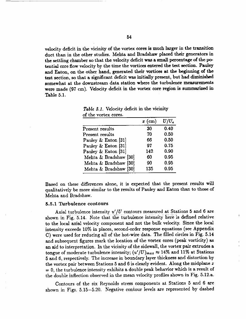
54
velocity deficit in the vicinity of the vortex cores is much larger in the transitionduct than in the other studies. Mehta and Bradshaw placed their generators in
the settling chamber so that the velocity deficit was a small percentage of the po-
tential core flow velocity by the time the vortices entered the test section. Pauley
and Eaton, on the other hand, generated their vortices at the beginning of the
test section, so that a significant deficit was initially present, but had diminished
somewhat at the downstream data station where the turbulence measurements
were made (97 cm). Velocity deficit in the vortex core region is summarized in
Table 5.1.
Table 5.1. Velocity deficit in the vicinity
of the vortex cores.
x (cm) v/u,Present results 30 0.40
Present results 70 0.50
Pauley & Eaton [31] 66 0.50
Pauley & Eaton [31] 97 0.75
Pauley & Eaton [31] 142 0.90
Mehta & Bradshaw [30] 60 0.95
Mehta & Bradshaw [30] 90 0.95
Mehta & Bradshaw [30] 135 0.95
Based on these differences alone, it is expected that the present results will
qualitatively be more similar to the results of Pauley and Eaton than to those of
Mehta and Bradshaw.
5.5.1 Turbulence contours
Axial turbulence intensity u'/U contours measured at Stations 5 and 6 are
shown in Fig. 5.14. Note that the turbulence intensity here is defined relative
to the local axial velocity component and not the bulk velocity. Since the local
intensity exceeds 10% in places, second-order response equations (see Appendix
C) were used for reducing all of the hot-wire data. The filled circles in Fig. 5.14
and subsequent figures mark the location of the vortex cores (peak vorticity) as
an aid to interpretation. In the vicinity of the sidewall, the vortex pair extrudes a
tongue of moderate turbulence intensity; (u'/U)mat ,,_ 14% and 11% at Stations
5 and 6, respectively. The increase in boundary layer thickness and distortion by
the vortex pair between Stations 5 and 6 is clearly evident. Along the midplane z
= 0, the turbulence intensity exhibits a double peak behavior which is a result of
the double inflection observed in the mean velocity profiles shown in Fig. 5.12.a.
Contours of the six Reynolds stress components at Stations 5 and 6 are
shown in Figs. 5.15-5.20. Negative contour levels are represented by dashed
55
lines. The level of symmetry for each stress component about the mldplane
z/R -- 0 is very good, even for the dit_cult-to-measure U'_ stress component
shown in Fig. 5.20. As expected, the _ and _ stress components change sign
between Quadrants 1 and 2. In general, Figs. 5.15-5.20 show that the Reynolds
stress contours are more distorted at Station 6 than at Station 5, and that peak
contour values are higher and displaced farther from the duct sidewall. The
increase in peak magnitude of the stresses is in contrast .to the decrease in peak
axial turbulence intensity (Fig. 5.14) which resulted from an increase in the local
axial velocity in the vicinity of the high turbulence levels.
At both Stations 5 and 6, the peak magnitude of the transverse normal stress
components v 2 and w 2 are ne___r equal and are roug____ half the peak magnitude
of the axial stress component u 2. Qualitatively, the u 2 stress component differs
significantly between all the vortex studies. The results of Mehta and Bradshaw
at 135 cm show that as the wall is approached along the plane of symmetry, the
u 2 component monotonically increases. The results of Pauley and Eaton at 97
cm show a peak in the near-wall region, but also show an additional peak on
the plane of symmetry near the outer edge of the vortices. They also show a
pair of peaks in the vortex core region symmetrically located about the plane
of symmetry. The present results show a large peak on the plane of symmetry
at the edge of the vortex pair. These differences can be traced to the velocity
deficit (or lack of) in the vortex core re, on. It is likely that the vortices in the
Pauley and Eaton study exhibited similar behavior to the present results at a
location closer to the generators since a large velocity deficit is present__directly
behind the generators. At Station 6, the present results show that the w 2 stress
component exhibits two peaks symmetrically located about the y--0 midplane
which were not observed at Station 5. Pauley and Eaton's data at 97 cm suggest
that all the normal stresses will eventually exhibit this double peak behavior.
Anisotrop_y bet._.ween the axial stress component and the horizontal transverse
component (u 2 - v 2) is shown in Fig. 5.21. At Station 5, the axial component is
everywhere larger than the horizontal component. In the vicinity of the vortex
core at Station 6, however, the transverse component exceeds the axial compo-
nent by as much as 20%. This is in contrast to a two-dimensional boundary layer
where the axial component is greater than either transverse components. Pauley
& Eaton and Mehta & Bradshaw both report similar behavior of the normal
stresses in the vicinity of the vortex core. Anisotropy between the axial and ver-
tical normal stress components (u 2 - w 2)) is shown in Fig. 5.22. Near the vortex
core at Station 5, the stresses are observed to be nearly equal. In the vicinity
of y/R = 1.4, =l:z/R = 0.35, the vertical stress exceeds the axial component. At
Station 6, the vertical stress is everywhere less than the axial component, but
they are still nearly equal in the vortex core region. Anisotro__py be..._tween the ver-
ticai and horizontal transverse normal stress components (v 2 - w 2) is important
in the generation of streamwise vorticity in non-circular ducts (see Section 5.4.1).
56
Contours of this quantity are plotted in Fig. 5.23. These plots show significant
differences between Stations 5 and 6. It is well known that in two-dimensional
boundary layers, u-_ > u-'_ > u"_, where u-_ is the axial component, u-_ is the
transverse component tangential to the surface, and u_ is the component which
acts normal to the surface (see, e.g., Fig. 18.5 of Ref. 54). For the transition
duct flow, the above inequality is observed to hold true in the near-wall region at
both Stations 5 and 6. In the outer region of the upper and lower wall boundary
layers at Station 5, however, the component tangent to the surface exceeds the
component which acts normal to the surface (negative anisotropy). In the region
of the vortex pair at Station 5, a small pocket exists where the auisotropy is pos-
itive. By Station 6, the region of positive anisotropy has grown and intensified.
The results at Station 6 are qualitatively very similar to the results reported by
Pauley and Eaton for a vortex pair at a development length of 97 cm (see Fig.
4.39 of Ref. 31).
The primary shear stress _ shown in Fig. 5.18 is observed to be positive
everywhere except for a small region in the vicinity of the vortex cores. These
regions of negative stress are a result of the positive mean rate-of-strain (OU/Oy >
0) associated with the aforementioned velocity ridge (see Section 5.4.3). Along
the midplane z=0 where the axial mean velocity profile flattens, the primary
mean rate-of-strain in both the y and z directions is nearly zero and, as a result,
stress levels in this region are depressed. In the z-direction, the primary shear W_
shown in Fig. 5.19 also changes sign as the summit of the velocity ridge is crossed.
The secondary shear stress _ is another quantity that plays an important role
in the production of streamwise vorticity (see Section 5.4.1). In the vicinity of
the vortex cores, this stress is of the same order of magnitude as the primary
shear stresses.
The normal stress data were used to calculate the turbulence kinetic energy.
These results are shown for Stations 5 and 6 in Fig. 5.24. The production of
kinetic energy was also calculated. Neglecting streamwise derivatives, the pro-
duction of kinetic energy is given by:
OU OU
P = - --uw (5.3)
Contours of this quantity are shown in Fig. 5.25. Generally, high levels of kinetic
energy are associated with high production rates. A notable exception occurs
on the duct upper and lower walls at Station 5. Here, the production in the
near-wall region is significantly less than that observed at Station 6, which seems
disproportionate when compared to the relatively small difference in kinetic en-
ergy between these stations. Between Stations 5 and 6, the peak production
is essentially the same, but the peak kinetic energy increases by approximately
35%.
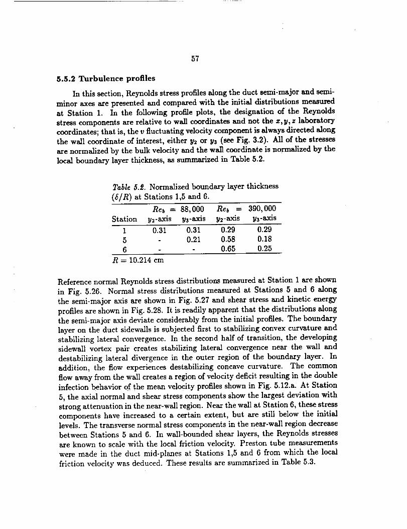
57
5.5.2 Turbulence profiles
In this section, Reynolds stress profiles along the duct semi-major and semi-
minor axes are presented and compared with the initial distributions measured
at Station 1. In the following profile plots, the designation of the Reynolds
stress components are relative to wall coordinates and not the x, y, z laboratory
coordinates; that is, the v fluctuating velocity component is always directed along
the wall coordinate of interest, either y2 or Ys (see Fig. 3.2). All of the stresses
are normalized by the bulk velocity and the wall coordinate is normalized by the
local boundary layer thickness, as summarized in Table 5.2.
Table 5._. Normalized boundary layer thickness
(b/R) at Stations 1,5 and 6.
Reb -" 88,000 Reb = 390,000
Station y2-axis ys-axis y2-axis ys-axis
1 0.31 0.31 0.29 0.29
5 - 0.21 0.58 0.18
6 - - 0.65 0.25
R = 10.214 cm
Reference normal Reynolds stress distributions measured at Station 1 are shown
in Fig. 5.26. Normal stress distributions measured at Stations 5 and 6 along
the semi-major axis are shown in Fig. 5.27 and shear stress and kinetic energy
profiles are shown in Fig. 5.28. It is readily apparent that the distributions along
the semi-major axis deviate considerably from the initial profiles. The boundary
layer on the duct sidewalls is subjected first to stabilizing convex curvature and
stabilizing lateral convergence. In the second half of transition, the developing
sidewall vortex pair creates stabilizing lateral convergence near the wall and
destabilizing lateral divergence in the outer region of the boundary layer. In
addition, the flow experiences destabilizing concave curvature. The common
flow away from the wall creates a region of velocity deficit resulting in the double
infection behavior of the mean velocity profiles shown in Fig. 5.12.a. At Station
5, the axial normal and shear stress components show the largest deviation with
strong attenuation in the near-wall region. Near the wall at Station 6, these stress
components have increased to a certain extent, but are still below the initial
levels. The transverse normal stress components in the near-wall region decrease
between Stations 5 and 6. In wall-bounded shear layers, the Reynolds stresses
are known to scale with the local friction velocity. Preston tube measurements
were made in the duct mid-planes at Stations 1,5 and 6 from which the local
friction velocity was deduced. These results are summarized in Table 5.3.
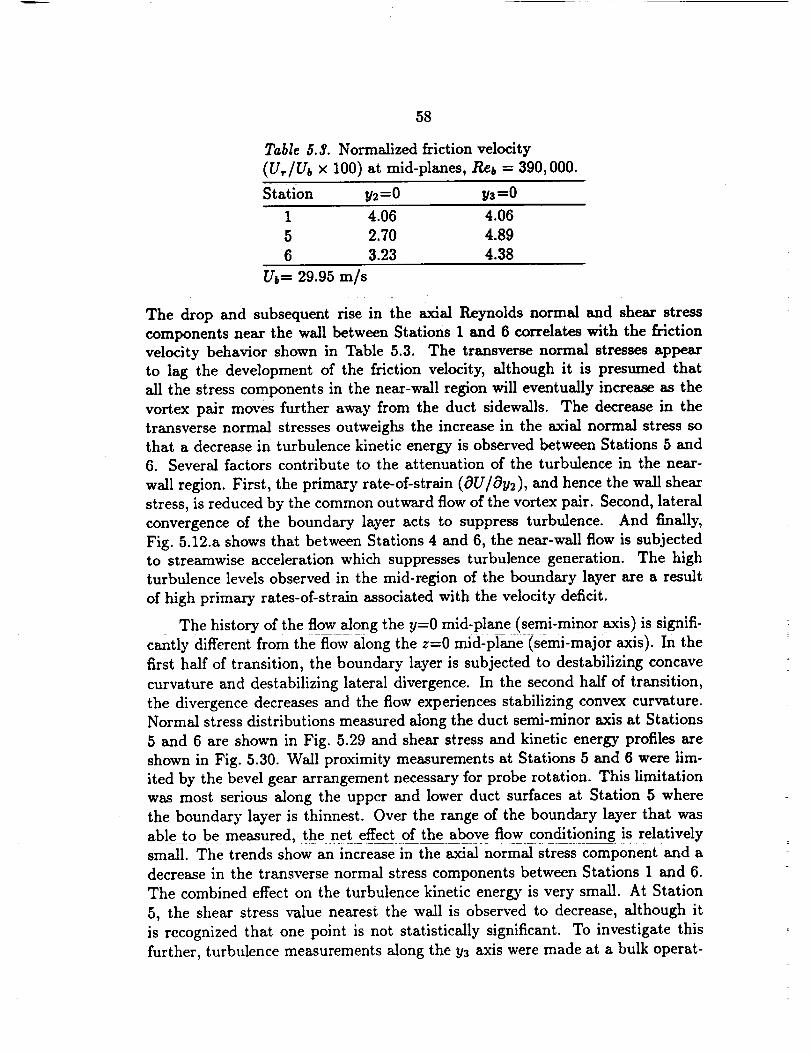
58
Table 5.8. Normalized friction velocity
(U,./U, x 100) at mid-planes, Reb = 390,000.
Station y2 =0 ys =0
1 4.06 4.06
5 2.70 4.89
6 3.23 4.38
Ub= 29.95 m/s
The drop and subsequent rise in the axial Reynolds normal and shear stress
components near the wall between Stations 1 and 6 correlates with the friction
velocity behavior shown in Table 5.3. The transverse normal stresses appear
to lag the development of the friction velocity, although it is presumed that
all the stress components in the near-wall region will eventually increase as the
vortex pair moves further away from the duct sidewalls. The decrease in the
transverse normal stresses outweighs the increase in the axial normal stress so
that a decrease in turbulence kinetic energy is observed between Stations 5 and
6. Several factors contribute to the attenuation of the turbulence in the near-
wall region. First, the primary rate-of-strain (aU/ay2), and hence the wall shear
stress, is reduced by the common outward flow of the vortex pair. Second, lateral
convergence of the boundary layer acts to suppress turbulence. And finally,
Fig. 5.12.a shows that between Stations 4 and 6, the near-wall flow is subjected
to streamwise acceleration which suppresses turbulence generation. The high
turbulence levels observed in the mid-region of the boundary layer are a result
of high primary rates-of-strain associated with the velocity deficit.
The history of the flow along the y=O mid-plane (semi-minor axis) is signifi-
cantly different from the flow along the z=O mld'pl_e (semi-major axis). In the
first half of transition, the boundary layer is subjected to destabilizing concave
curvature and destabilizing lateral divergence. In the second half of transition,
the divergence decreases and the flow experiences stabilizing convex curvature.
Normal stress distributions measured along the duct semi-minor axis at Stations
5 and 6 are shown in Fig. 5.29 and shear stress and kinetic energy profiles are
shown in Fig. 5.30. Wall proximity measurements at Stations 5 and 6 were lim-
ited by the bevel gear arrangement necessary for probe rotation. This limitation
was most serious along the upper and lower duct surfaces at Station 5 where
the boundary layer is thinnest. Over the range of the boundary layer that was
able to be measured, the net effect of the above flow conditioning is relatively
small. The trends show an increase in the axial normal stress component and a
decrease in the transverse normal stress components between Stations 1 and 6.
The combined effect on the turbulence kinetic energy is very small. At Station
5, the shear stress value nearest the wall is observed to decrease, although it
is recognized that one point is not statistically significant. To investigate this
further, turbulence measurements along the y3 axis were made at a bulk operat-
59
ing Reynolds number of 88,000 where the boundary layer is thicker and a larger
region could be resolved. Shear stress and kinetic energy profiles for this case are
shown in Fig. 5.31. These results confirm both the unchanged kinetic energy lev-
els and the decreasing behavior of the shear stress. The decrease in shear stress
is in contrast to the increased wall shear stress measm_ by means of the Preston
tubes. This indicates that either the shear stress recovers in the near-wall region
or that the flow is not in local equilibrium near the wall. Without the benefit of
turbulence measurements at the intermediate Stations 3 and 4, it is difficult to
speculate on the factors which lead to the flow condition at Station 5. Near-wall
behavior will be examined more closely in Section 5.7.
6.6 Turbulence Modelling Considerations
The inviscid calculations by Burley et al. [7,8] have shown that even for
overall performance predictions, viscous effects cannot be neglected when calcu-
lating transition duct flows. For accurate predictions the effects of turbulence
must also be included. The level of turbulence modelling required, of course,
depends on the information desired. From a computational standpoint, the most
difficult aspect of the present configuration is the flowfleld in the neighborhood of
the vortex pair. Since the initial generation of streamwise vorticity via pressure
gradient effects is essentially an inviscid process, even simple models will predict
the presence of the vortex pairs. Accurate prediction of the diffusion of vortic-
ity, however, relies on accurate modelling of the Reynolds stress components.
Modelling efforts for the present configuration can be divided into two groups.
The first group is concerned primarily with overall performance parameters and
prediction of flow separation. The computational work of Liandr_t et al. [33] has
shown that the primary features of the mean flowfield in the region of embedded
vortices can be predicted reasonably well with simple mixing length models. The
second group is concerned with the task of demonstrating the ability of particular
turbulence models to predict detailed mean flow and Reynolds stress behavior.
The present data set should be useful for this group.
The simplest turbulence model is the algebraic (zero-order) eddy viscosity
model based on the concept of Boussinesq. Here, the Reynolds stresses are
assumed to behave like the molecular viscosity stresses and the Reynolds stress
tensor for incompressible flow is written as:
.OUi OUj . 2 (5.4)
where vt is the turbulent eddy viscosity, /_ii is the Kronecker delta function
and k is the turbulence kinetic energy. Equation (5.4) is applicable to three-
dimensional flows where only the Reynolds shear stresses (u--7_', i # j) are
important, inasmuch as the Reynolds normal stresses predicted by this equation
are not in agreement with even simple flows. For the present configuration,
6O
equation (5.4) may be adequate for prediction purposes through the end of the
transition section, but will not be applicable if the flow is allowed to develop in the
rectangular duct where the transverse Reynolds normal stresses are important
in the generation and diffusion of corner-generated secondary flows.
Since many design-oriented flow solvers are implemented with algebraic eddy
viscosity turbulence models, it is worthwhile to examine the behavior of the
eddy viscosity for the present flow. For the primary shear stresses, if streamwise
gradients are neglected, equation (5.4) reduces to:
OU
= (5.5)OU
= (5.6)
Rearranging these equations to solve for the eddy viscosity yields:
=
v,,, = _ l(OV)Oz
(5.7)
(5.8)
where the y and z subscripts admit directional dependence (anisotropy) of the
eddy viscosity. The behavior of the primary rates-of-strain (denominators in
equations (5.7) and (5.8)) at Station 5 is shown in Fig. 5.32. Also indicated in
these plots are horizontal traverses along which the component eddy viscosities
were calculated. These results, plotted in terms of a viscosity ratio (vt/v), are
shown for Station 5 in Fig. 5.33. Equivalent results for Station 6 are shown
in Figs. 5.34 and 5.35. To avoid singular points where the strain-rates vanish
(between solid and dashed lines in Figs. 5.32 and 5.34), the eddy viscosity is
computed only where the denominator in equations (5.7) and (5.8) is greater
than 5% of its maximum value in the cross plane. Although the eddy viscosity
distributions shown in Figs. 5.33 and 5.35 show similar trends with respect to
symmetry about the midplane z=O, the magnitude of the differences is enough so
that the results should be considered only qualitative, In areas where the stress
and strain in both transverse directions are nominally of the same magnitude,
the eddy viscosity components are observed to be nearly equal. Most of the
regions where large deviations occur can be traced to either a large difference
in the component strain rates or to inadequate resolution of a large velocity
gradient, e.g., in the vicinity of the velocity ridge near the vortex core. this flow.
This is in contrast to the results of Mehta and Bradshaw, who reported that the
vt,y component in their embedded vortices was so ill-behaved so as to preclude
plotting.
61
It was mentioned in Chapter 2 that boundary layer flows with extra rates-of-
strain often exhibit more spectacular behavior than what is predicted by explicit
terms which account for the extra strain rates. It is argued that the reason for
this is that the extra rates-of-strain cause large changes in hlgher-order terms
which appear in the Reynolds stress transport equations. These higher-order
terms are modelled in terms of the Reynolds stresses and require the specification
of empirical constants. Dimensionless turbulence structure parameters such as
the cross-correlation coefficient are related to constants in turbulence models.
Often the constants are determined based on the results of simple flows such as
two-dlmensional boundary layers, resulting in poor performance when applied
to more complex flowfields. Some of these dimensionless structure parameters
were computed for the present flow. The shear stress correlations R_v = _'_/ulv ',
Ruw = _"w/u_w ' and Rvw = _-'_/v'w' evaluated at Stations 5 and 6 are shown
in Figs. 5.36, 5.37 and 5.38, respectively. The primary shear stress correlations
R,,_ and R,w may be compared with the two-dimensional value of 0.45. Near
the duct sidewalls and in the vicinity of the vortex cores, the R,_ parameter is
depressed due to strong lateral convergence of the boundary layer. At Station
5, in the region where the peak turbulence intensities occur, a near constant
value of approximately 0.55 is observed. By Station 6, the value has decreased
and is close to the two-dimensional value. Near the upper and lower walls, the
R,,w parameter generally is in agreement with the two-dimensional value. The
secondary shear stress correlation Rvw = _"_/v'w' at both stations shows values
in the range of 0.25 for most of the flowfield, but this parameter is also depressed
in the region of the vortex core. Another dimensionless parameter of interest
is the shear-energy ratio parameter al. This parameter is defined as the ratio
of the resultant shear stress in a plane normal to a wall surface to twice the
turbulence kinetic energy. In a two-dimensional boundary layer, this parameter
has also been observed to be constant with a value of 0.15 (see, e.g., Bradshaw
et al. [56]). For the present flow, two shear-energy parameters were computed:
aly = x/_'fi 2 + _"_2 /2k (5.9)
(5.10)
which are applicable away from the corner region on the vertical and horizontal
walls, respectively. The al v shear-ratio parameter at Stations 5 and 6 is shown
in Fig. 5.39 and the al= parameter is shown in Fig. 5.40. In the regions where
high turbulence levels are observed, the al_ parameter is higher than the two-
dimensional value and, like the shear stress correlation, is well below the initial
value in the region of the vortex pair. Along the horizontal walls, the alz param-
eter is elevated at Station 5, but returns to the initial value at Station 6. These
results show that the transition duct produces a distortion of the turbulence
structure, more so at Station 5 than at Station 6. The largest distortion occurs

62
in the vicinity of the vortex core region where lateral convergence suppresses
turbulence.
Further insight into the structure of the turbulence can be gained by exam-
ining the data in terms of the invariants of the anisotropic stress tensor. This
analysis is based on the concept of physical realizability limits of turbulence
which has been used extensively to study the return to isotropy of homogeneous
turbulence (see, e.g., Lumley [57]). The anisotropic stress tensor, first proposed
by Rotta [58], is defined as:
u, i- }k6, (5.11)bij = 2k
This tensor must satisfy the Cayley-Hamilton theorem:
_3 _ I_2 + II), - III = 0 (5.12)
where I,II and III are the tensor invariants:
I = bii
1II = --bi, b,i
2 d J
III = _bi._b._kbk_
The first invariant, I, is identically zero by definition of the turbulence kinetic en-
ergy. Invariant III defines the shape of the ellipsoid associated with the Reynolds
stress tensor. A positive value of III indicates that there is only one principle
component that is large, and a negative value indicates that two principle com-
ponents are large. Limits on the anisotropic stress tensor can be defined by
applying the condition that the Reynolds stress in any direction must go to zero
as the strain rate in that direction goes to infinity. For example, as OU/Oz goes
to infinity, u--_ goes to zero and bll goes to -1/3. The largest level of turbulence
that can occur in any one direction is 2k, which occurs when them turbulence is
one-dimensional. If all the turbulence is in the z direction, then u 2 = 2k and bl 1
is equal to 2/3. Following Lumley [571, the limits on allowable turbulence are
recast in terms of the tensor invariants II and III. These limits are illustrated
in Fig. 5.41. The shaded area on this plot represents the region within which all
physically realizable turbulence must lie. The nature of the turbulence at the
boundaries is also labeled. The Reynolds stress tensor at Stations 1, 5 and 6 was
recast in terms of the anisotropic stress tensor invariants. At Station I, the tur-
bulence is primarily contained in the axial component so it is expected that the
III invariant will always be positive. The invariants at Station 1 are plotted in
Fig. 5.42.a. Following Pauley and Eaton, the location of each data point on the
63
invariant map relative to its position in the flowfield is represented by a vector
which has its origin at II -" III= 0 and the tip at the data point location on the
invariant map. This vector is plotted with its origin coincident with the physical
location in the flowfield in Fig. 5.42.b. As expected, all the points correspond
to positive III values. At the edge of the boundary layer the turbulence should
approach an isotropic condition (zero vector length). The large vectors near the
boundary layer edge indicate that the turbulence is approaching a more one-
dimensional nature which is not realistic. This should not be taken to seriously
though, since the magnitude of the vector is not related to the magnitude of the
turbulence. That is, experimental uncertainty in regions of low-turbulence levels
can cause one component to be large relative to another resulting in an apparent
high level of anisotropy. Invariant map plots of the Reynolds stress data at Sta-
tions 5 and 6 are shown in Figs. 5.43 and 5.44, respectively. All of the data are
observed to lie within the limits of realizability. In the region of the vortex core,
the turbulence is nearly isotropic. In regions where the primary strain rates are
large, the turbulence structure is much like that of the initial two-dimensional
boundary layer at Station 1. Along the velocity ridge, where the primary strain
rates are small, the III invariant is negative. Between Stations 5 and 6 the data
cluster more toward and spread further out along the axisymmetric contraction
limit indicating that the axial stress component is becoming more dominant.
5.7' Wall Function Behavior
The use of wall functions for predicting the present flow was analyzed at
Stations 5 and 6. Reference coordinates for this analysis are shown in Fig. 5.45.
Since flow variables in the near-wall region scale with the local friction velocity,
peripheral skin friction coefficient distributions were obtained at Stations 5 and
6. These distributions, which were deduced from Preston tube data measured
along the periphery of the duct in Quadrant 1 (see Fig. 5.45), are shown in Fig.5.46. The results based on different diameter Preston tubes at Station 5 show
systematic variations with a change in diameter, particularly for s/s,.el < 0.6, in-
dicating that deviations from the law-of-the-wall exist at this station. Although
only two Preston tubes were used at Station 6, the relatively good agreement
suggests that the flow recovers to law-of-the-wall behavior downstream. Bound-
ary layer profiles were measured along the y,, traverses (n=1,2,5,6,7,8) shown in
Fig. 5.45 with both pitot and hot-wire probes. Results obtained at Stations 5
and 6, plotted in law-of-the-wall coordinates, are shown in Fig. 5.47. The fric-
tion velocities used for these plots are based on the average distribution fines
shown in Fig. 5.46. The non-dimensional outside diameters of the individual
Preston tubes are superimposed on these plots. At Station 5, deviations from
the law-of-the-wall are apparent for y+ values greater than 80. In the near-wall
region, however, all profiles tend toward law-of-the-wall behavior within the in-
terval 30 < y+ <_ 80. At Station 6, the law-of-the-wall is satisfied on all traverses
for y+ values between 30 and 200. This behavior implies that the law-of-the-wall
64
may be used for prediction purposes, recognizing that the limiting y+ value on
the first mesh line between the duct inlet (Station 1) and Station 5 may be less
than the limiting value which applies at Station 5 (y+ -_ 80).
Wall function behavior for the turbulence kinetic energy (k) and the dissi-
pation rate of turbulence kinetic energy (e) was also analyzed at Stations 5 and
6. If only first-order effects are retained and terms containing secondary rates-
of-strain are neglected in the reduced forms of the Reynolds stress transport
equations, and the mean velocity profile along any normal to the duct surface
is in accordance with the law-of-the-wall, then the following expressions (rela-
tive to the xw,y_,,zw wall coordinate system) apply for turbulent flow through
non-circular ducts in local equilibrium [59]:
(5.13)
(5.14)
(5.15)
where
(5.16)Fp= 1+
with C_, = 0.09 and _¢ = 0.41, and where Ip is Prandtl's length scale. In the near-
wall region along the transition duct horizontal and vertical walls at Stations 5
and 6, (OU/Oyw) _ (OU/Ozw), so that Fp _- 1.0. Further, it is reasonable to
assume that along these walls, but excluding the corner region, Prandtl's length
scale can be specified as Ip=tcy_. With these assumptions, the following alternate
forms of equations (5.13)-(5.15) apply along the horizontal and vertical walls:
k 1
Pyw 1
V$
(5.17)
(5.18)
= 1 (5.19)
where e has been replaced by P (production) in accordance with the local equilib-
rium assumption. Distributions of x/_-_ 2 + _'_2/U_, k/V_ and Py_/U_ along
several traverses parallel to the z axis at Stations 5 and 6 are shown in Figs. 5.48,
5.49 and 5.50, respectively. Also indicated on these plots are the conventional
65
wall function values. Although the results are restricted to y+ values greater
than 400 because of limitations imposed by the probe rotation mechanism, some
conclusions can still be drawn. For example, it can be seen that distributions
measured along the vertical midplane traverse y/R = 0 at Stations 5 and 6 gen-
erally tend toward the conventional limits. This same comment applies for all
other distributions measured at Station 6. At Station 5, however, the trends are
more difficult to discern, especially along the y/R -- 1.37 traverse, which lies
within the sidewall boundary layer.
The behavior of _/h'_ 2 + _-_2/U_, k/U_ and Py/U_ along the semi-major
traverse y2 = 0 at Stations 5 and 6 is shown in Figs. 5.51, 5.52 and 5.53, respec-
tively. The distributions measured at Station 6 approach the conventional limits.
The deviation observed at Station 5 is probably attributable to the neglect of
secondary rates-of-strain in the derivation of equations (5.13)-(5.15), inasmuch
as Fig. 5.9 shows that secondary strain near the sidewall at Station 5 is a large
percentage of the primary rate-of-strain, but that it decreases to a relatively
small percentage by Station 6. The first data point for Station 5, however, is at
y+ _ 300 which is beyond the region where law-of-the-wall behavior is observed
(refer to the y+ distribution of Fig. 5.47.a). In reference to predictions, if y+
on the first mesh line is restricted to an interval between 30 and 50, and if sec-
ondary rates-of-strain are small within this interval, then wall function values on
this mesh line may be close to the conventional limits at Station 5 and, indeed,
at intermediate stations within the duct. Further measurements in the near-wall
region will be required in order to verify this conjectured behavior.
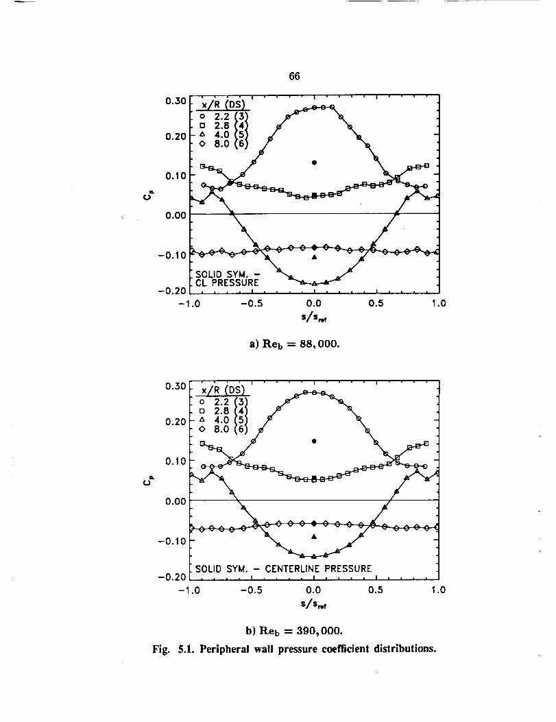
L
0
0.30
0.20
0.10
0.00
-0.10
x/R (DS)
o 2.8A 4.00 8.0
SOLID SYM. -CL PRESSURE
66
0.0 0.5
S/Star
a) Reb = 88,000.
es.
¢J
0.30
0.20
0.10
0.00
-0.10
' I I i
o 2.2 (3) ..,,_ _%._.o 2.S (4) _f '%,_= 4.0 (5) /_ %
SOLID SYM. - CENTERLINE PRESSURE
.0 -0.5 0.0 0.5
S/Sref
.0
b) R,eb = 390,000.
Fig. 5.1. Peripheral wall pressure coefficient distributions.
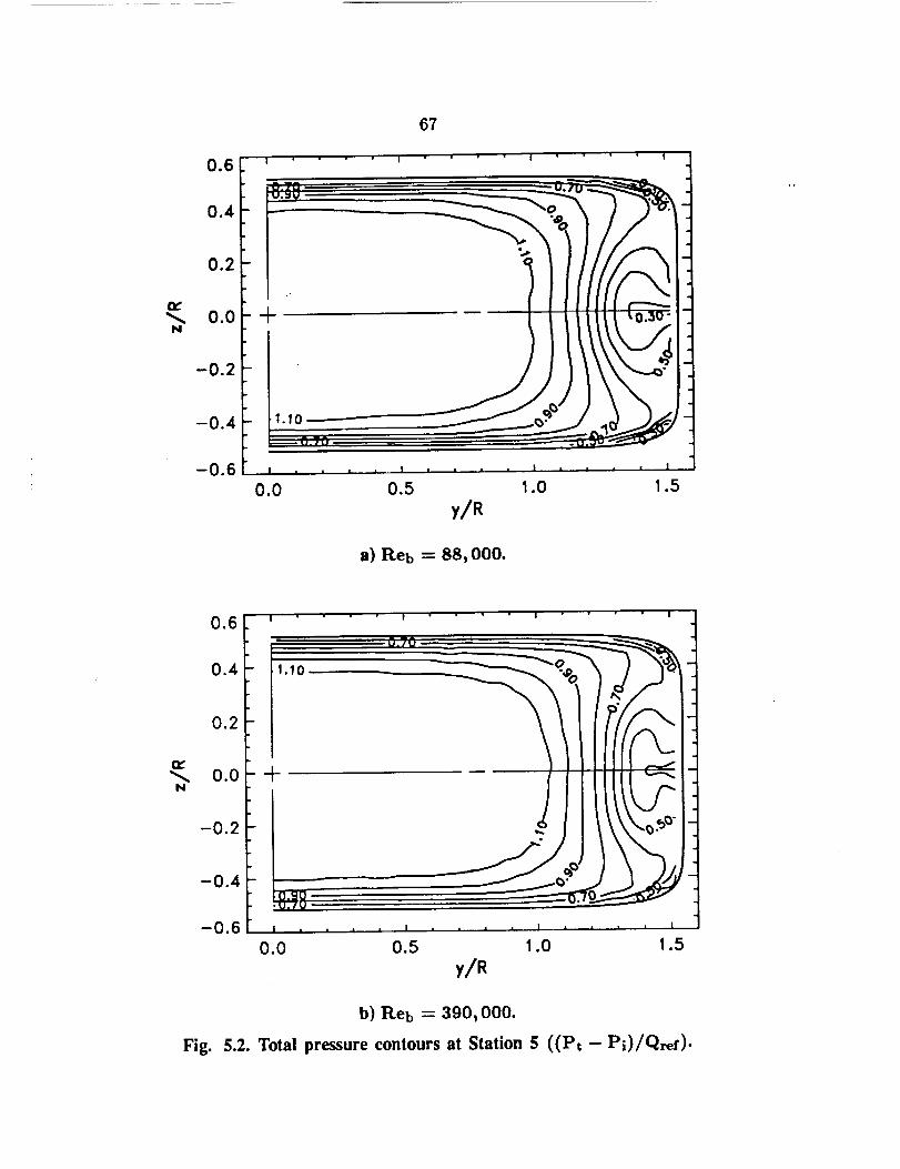
rv.
N
0.6
0.4
0.2
0.0
-0.2
-0.4
-0.6
I I
-t-I
iI
| |
0.0
67
• ' ' I ° !
I I a I I | i I I • I
0.5 1.0 1.5
y/R
a) Reb = 88,000.
it,,
N
0.6
0.4
0.2
0.0
-0.2
-0.4
-0.6
1.10
÷
D
m
,u:i_
! •
0.0
! !
a.70
.... --o.:
i = • |
0.5 1.0
y/R
I
I
. I
1.5
b) Reb = 390,000.
Fig. 5.2. Total pressure contours at Station 5 ((Pt - Pi)/Qref).
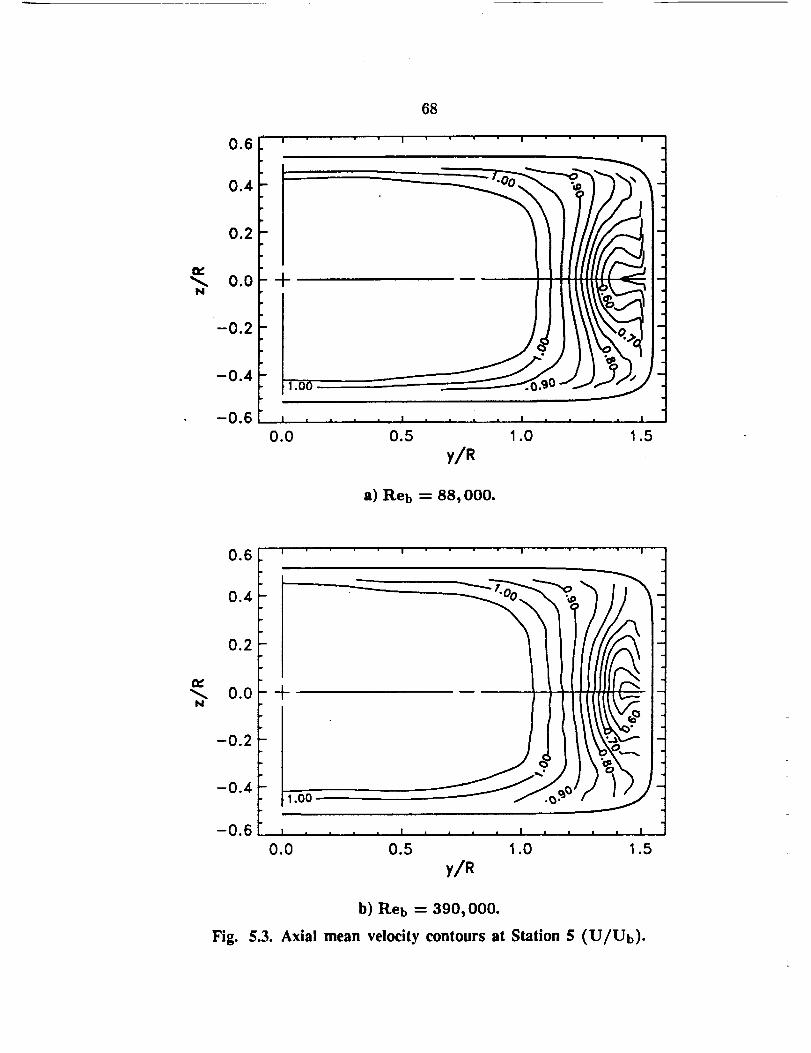
fv.
N
0.6
0.4
0.2
0.0
-0.2
-0.4
-0.6
+
1.00
0.0
68
a) Reb = 88,000.
1.0 1.5
N
0.6
0.4
0.2
0.0
-0.2
-0.4
-0.6
-t-
'l'
m
1.00
I
0.0
I I I
! .... 1 = . = • !
0.5 1.0 1.5
y/R
b) Reb = 390,000.
Fig. 5.3. Axial mean velocity contours at Station 5 (U/Ub).
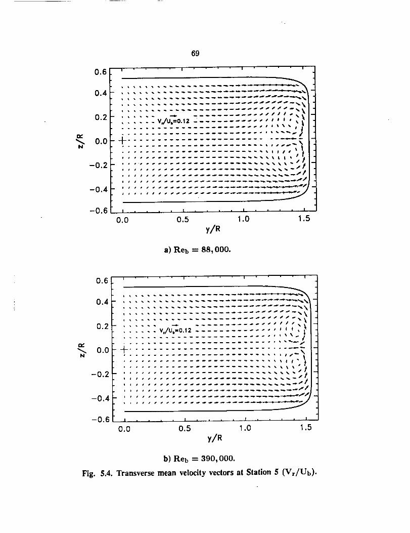
N
0.6
0.4
0.2
0.0
-0.2
-0.4
-0,6
69
I I " I a
,,-,, .. :: :--:-:-:::::::::_____... _.... V_/Ub=0.12 ....... / * J O _ _,
I ',_ I i. ! I , I I I I I I I I i
0.0 0.5 1.0 1.5
y/R
a) ]:{.eb = 88,000.
N
Fig.
0.6
0.4
0.2
0.0
-0.2
I I ' -- I I
: :::::: - :
...... V,/Ub=0.12 . , / i I _
, .... _
/
....................... ,,,,;_
-o.4i ....... ::::::::--,.:: ...... ----":'//-I
-0.6 _- "-"-"-" 2"_"_- _
0.0 0.5 1.0 1.5
y/R
b) Reb = 390,000.
5.4. Transverse mean velocity vectors at Station 5 (Vr/Ub).
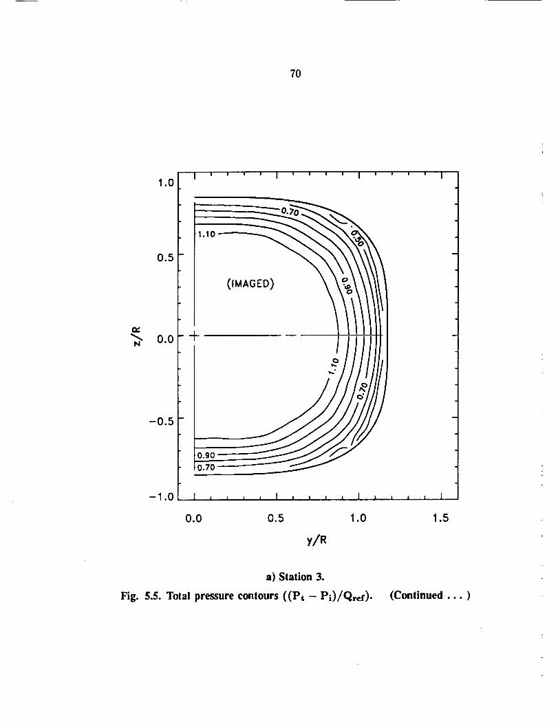
?0
1.0
0.5
_N 0.0
--0.5
--1.0
I ' ' ' ' I ""_ ' ' ' I '
I , , , , J I , , , I
0.0 0.5 1.0
y/R
I , I
' ' ' I
a) Station 3.
Fig. 5.5. Total pressure contours ((Pt - Pi)/Qref)- (Continued ... )
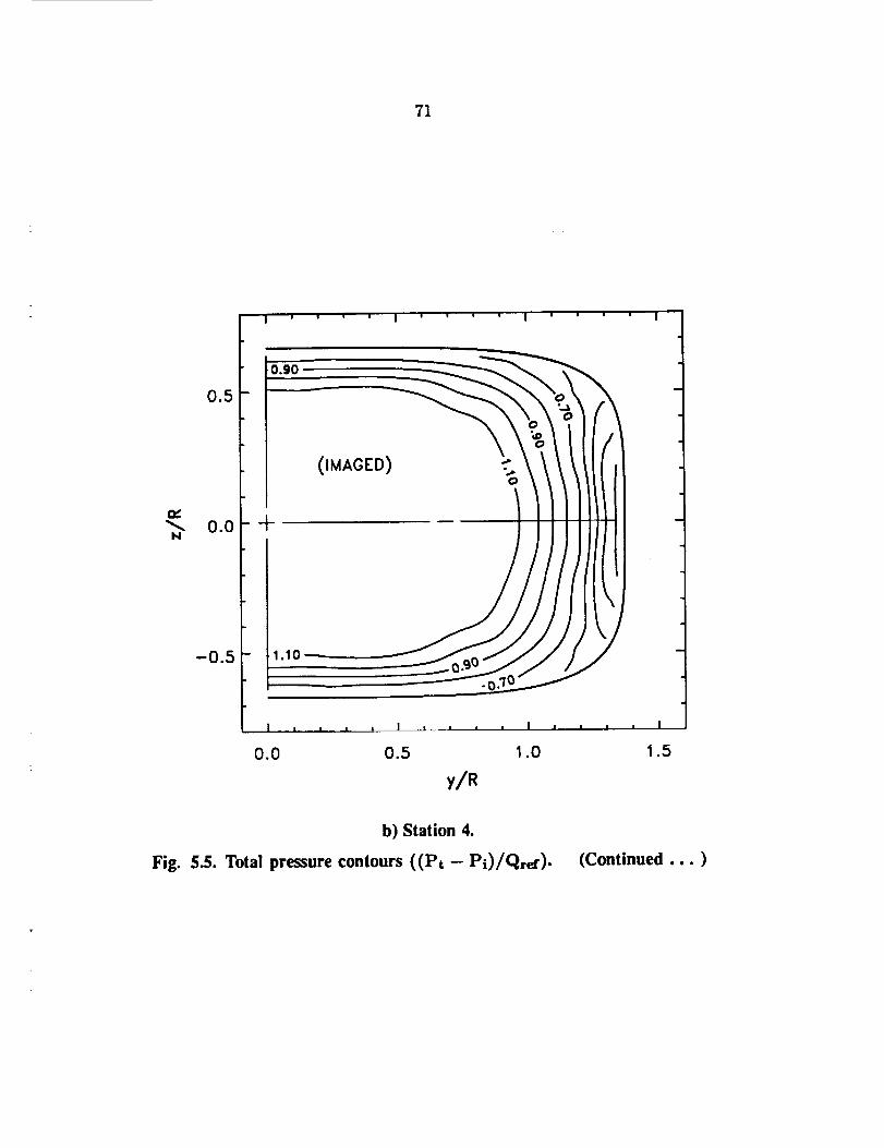
71
N
I ' .... I .... I ' ' '
0.90
0.5
o.o- +
-0.5 1.10
(IMAGE
I _ • . , I , . . . I , , . . I
0.0 0.5 1.0 1.5
y/R
b) Station 4.
Fig. 5.5. Total pressure contours ((Pt - Pi)/Qrd). (Continued ... )
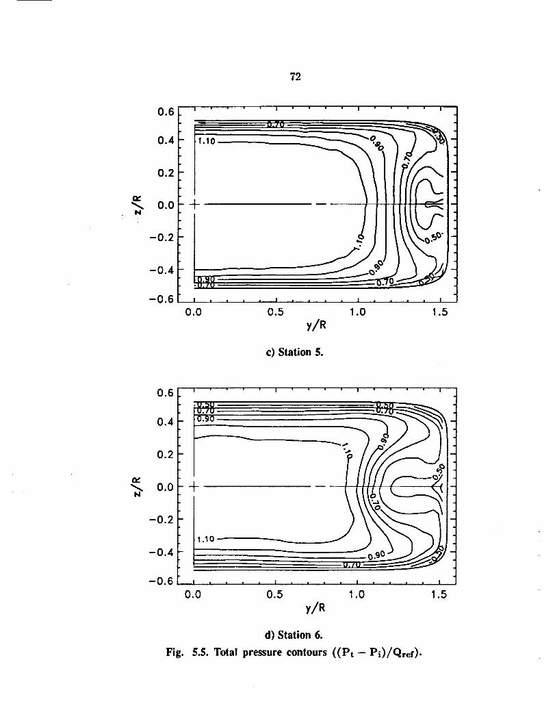
72
Lw_A|
N
0.6
0.4
0.2
0.0
-0.2
-0.4
-0.6
| •
- 1.10
+
0.9_Q
I I •
0.0
I I I.
! _ _ • • l • I
0.5 1.0 1.5
y/R
c) Station 5.
rv,
N
0.6
0.4
0.2
0.0
-0.2
-0.4
-0.6
"."U.DU
U./U0.90
I
-+
1
I
1.10
I _
0.0
I I I
-4
u._ " ;_-_--_-_".,
i i i I I I " " I • • • • !
0.5 1.0 1.5
y/R
d) Station 6.
Fig. 5.5. Total pressure contours ((Pt- Pi)/qref).
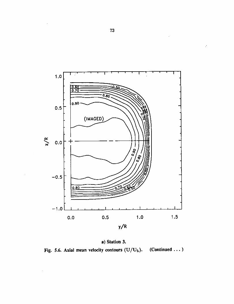
0.80
._._ y/_0.0
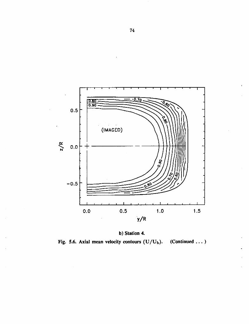
?4
0.5
n..0.0
N
-0.5
I ' ' ' ' i ' ' ' ' I ' ' ' ' l
I i i . i , J i i i ¢ | i i ' ' I
0.0 0.5 1.0 1.5
y/R
b) Station 4.
Fig. 5.6. Axial mean velocity contours (U/Ub). (Continued ... )
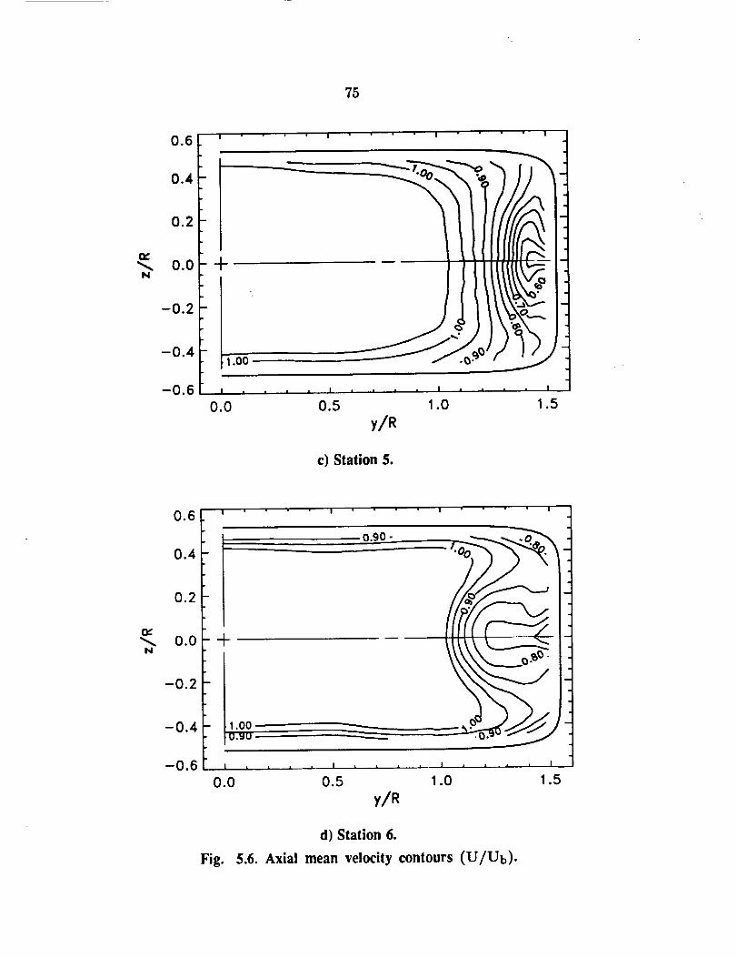
75
rr
N
0.6
0.4
0.2
0.0
-0.2
-0.4
-0.6
+
1.00
0.0 0.5
y/R
c) Station 5.
1.0 1.5
iv,
N0.0
0.90 -
1.00O.SU
0.0 0.5 1.0 1.5
y/R
d) Station 6.
Fig. 5.6. Axial mean velocity contours (U/Ub).
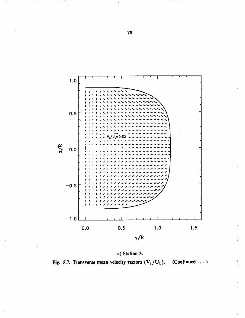
76
N
1.0
0.5
0.0
-0.5
-I .0
I ' ' ' ' i ' ' ' ' I '
t I •
% % % % ___
% % % % ___
r
v/uTo=.s2----............-
+so_
IIIstIsJs_s_J_JJJ_
IIIIIII lllillllll/
tl///tt1_Ill/fill
J I I .... J. J J • i I I J i
0.0 0.5 1.0
y/R
I !
a) Station 3.
Fig. 5.7. Transverse mean velocity vectors (Vr/Ub). (Continued ... )
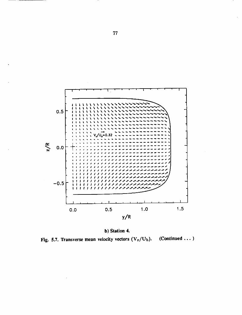
??
N
0.5
0.0
-0.5
i iiI .... I ' " " ' I .... I
.... -_-b=-.-- ........ •
I I I I I I I I I lillillll_I/
I t I t ttlttl
I I I I I I I/////11__
i I I I ' ] ' ' L , [ S i I
0.0 0.5 1.0
y/R
I
1.5
b) Station 4.
Fig. 5.7. Transverse mean velocity vectors (Vr/Ub). (Continued ... )
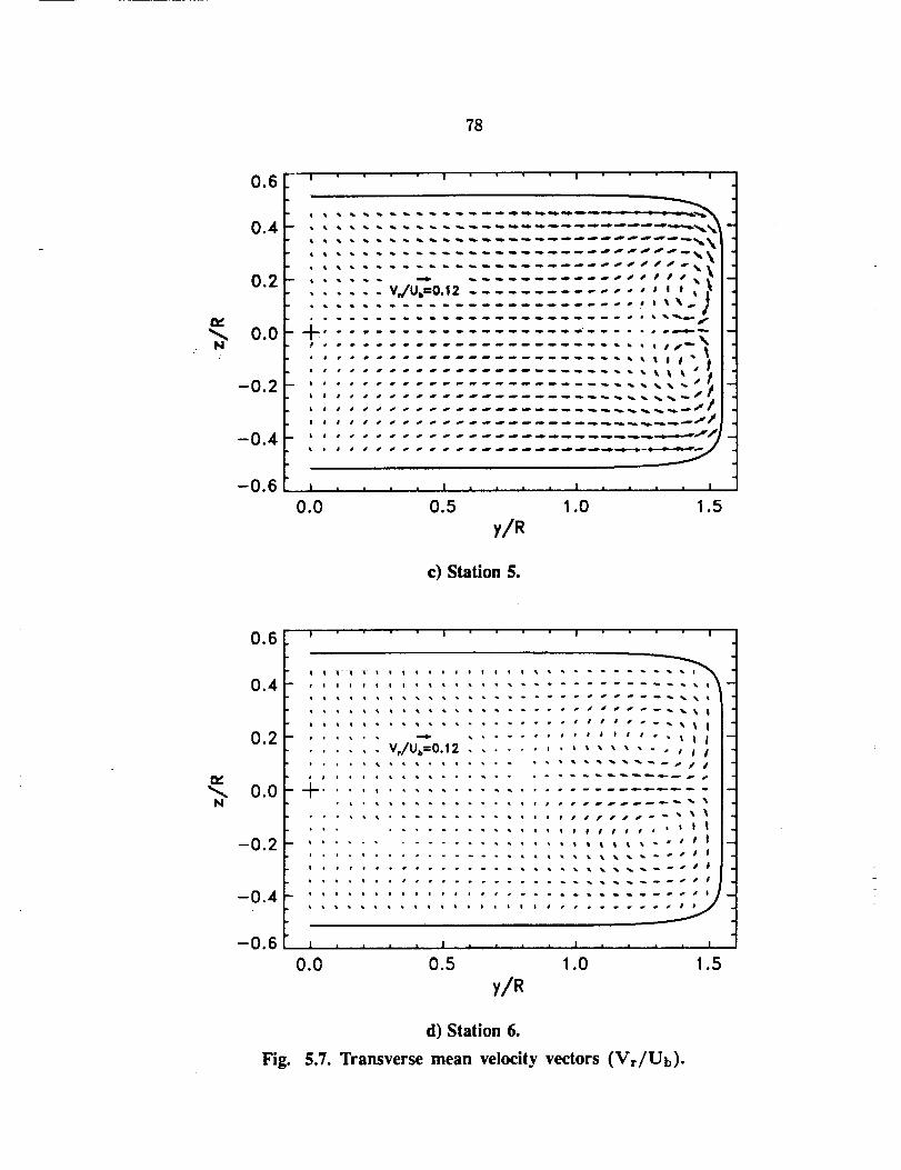
78
N
0.6
0.4
0.2
0,0
-0.2
-0.4
-0.6
I I I I
', : : - : .". : _:._Z-_.-=ZZZ=_-z_ -
..... i iiii!!ii! !!ill__._...,,,,_ -
•....._.. _+,...... _'i:..., _,
' i i .......... " " --" jiw
| | | ¢ ¢ i , , • . . . | . . . • i
0.0 0.5 1.0 1.5
x/R
c) Station 5.
m,,
N
0.6
0.4
0.2
0.0
-0.2
-0.4
-0.6
I I I I
.d_=_.,_ ....... _ _ • • • • # I
_ll
l I I " • J " " " " 1 • • j • I
0.0 0.5 1.0 1.5
d) Station 6.
Fig. 5.7. Transverse mean velocity vectors (Vr/Ub).

79
,6 I I " ' " " I I
0.4 , .- _" , o' . o I _-I 4," S/ # /I " ¢'_" | | ,
0.2 I ,' , , / / \ I_/ t I I I _ _ I.
I ',, , , ,, \ x... 1:-o.2 I---. ", ',, ', \ I I-
I "'-, % ", '.,o ", _._ _ I--o., I-o.,_-. "'. _', ", • ', % I J-
-0.6 , • , , , , . . . , ...... ,
0.0 0.5 1.0 1.5
y/R
a) Measured.
.6 I I I " ' I
0.4 °"12 ...--- ., <. _ )_ .
0.2 l'- - -" , ' ' ' I k"hl, _ I / / _ I _ II ^\ )A
r, , ., , ,' ', ?g- ) I I( hi _,--n^_--_ .' / _5 21 I _ u _\_r -.-,_...... . .---.0.0_.o.o,'---. ' ' , \ _ r,,(AJI .-. _ I l ,, \ C_ I o'_,v(
_. -,,. % %.-o.2 I , , , ' ' ", b__l i_ )1L ,..." _. I , ,/" %J ]//_I,
_, / ¢. .. II:," . ,. , ,,.9 -' Yn"AI-o.4 F:----- :: :£-' ," ,' ) ,-..,-f-__¢' v\l
!-o..o_-_:_=.__. , . _____-___ _.j--0.6 I , l l L t , I I 1 | ..... I I
0.0 0.5 1.0 1.5
WR
b) Calculated.
Fig. 5.8. Static pressure contours ((P - Pi)/qref) at Station 5.
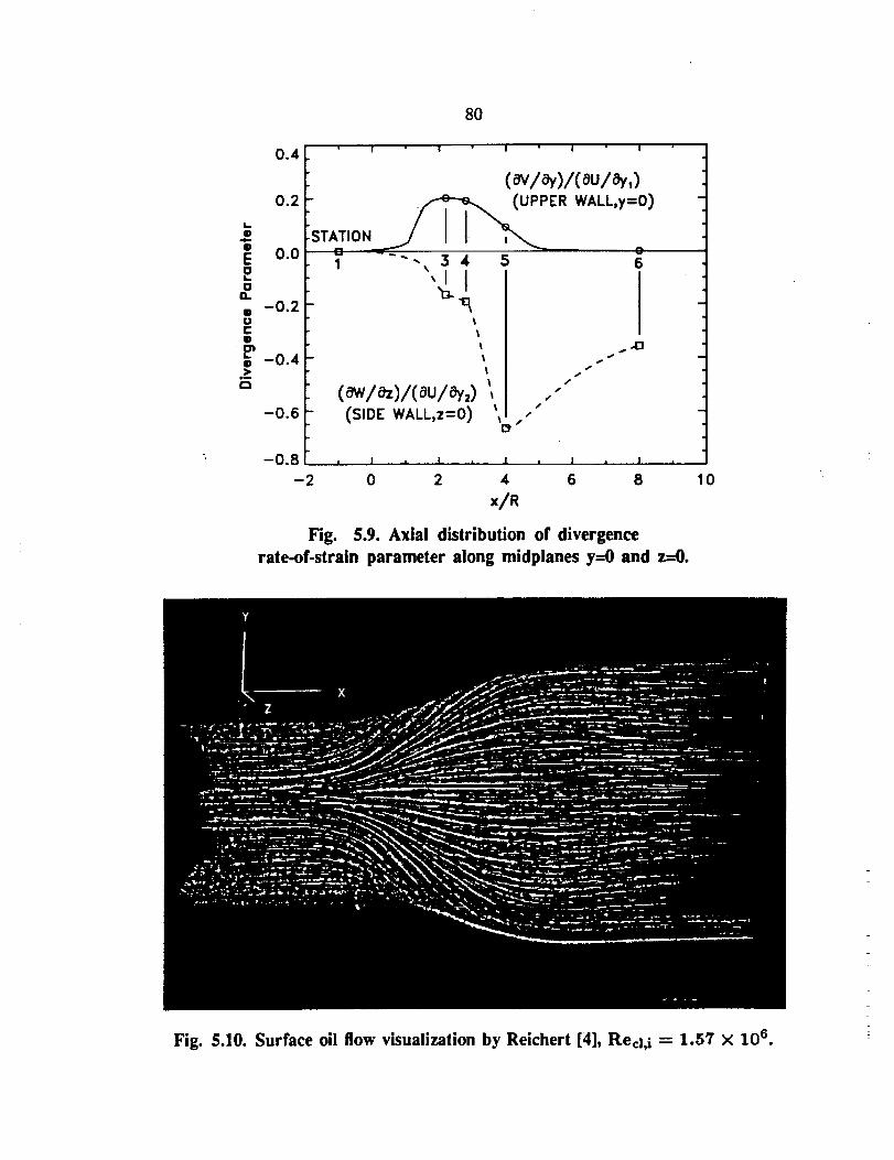
k.Q
O
EPg3
n
DUCQ
g
mr'_
80
0.4
0.2
0.0
-0.2
-0.4
-0.6
I I ! •
. _ER_STATION
-a.
I
I
I
(owl_)l(_ul_,) ', .(SIDE WALL,z=O) _ ,."
-0.8
-2 0
I I I
(w/o3,)/(ou/,_.,)WALL,y=O)
s/
0
6
......0s
s
2 4 6 8
x/R
Fig. 5.9. Axial distribution of divergence
rate-of-strain parameter along midplanes y--0 and z--0.
0
Fig. 5.10. Surface oil flow visualization by Reichert [4], Red,i -- 1.57 X 10 6.
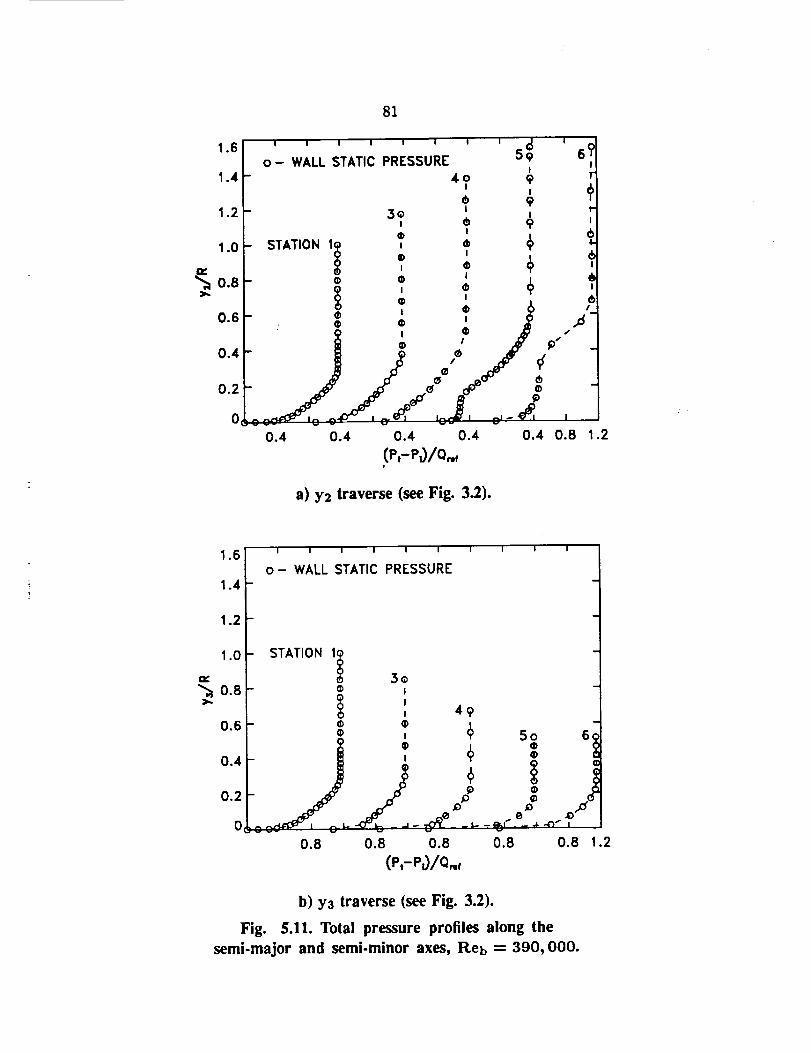
1.6
1.4
1.2
1.0
Jy
"_ 0.8)k.
0.6
0.4
0.2
0
81
I I I I I I l I i_ I
o- WALL STATIC PRESSURE 59I
- 40 9I9
- 3e9
- STATION 1 ® •
- ¢ • 1
• ¢ ¢
"j ,>. i I p"
0.4 0.4 0.4 0.4 0.4
(P,-P=)/Q=,
a) y2 traverse (see Fig. 3.2).
64IT
4>r
il
,4
"t!
0.8 1.2
1.6
1.4
1.2
1.0
ev,
0.8>,.
0.6
0.4
0.2
0
I I I I I I
o- WALL STATIC PRESSURE
I I I I
STATION 11 3e
_ ,_ 49¢ ¢ -
J2 ', ,
:__, _Z -°°0.8 0.8 0.8 0.8 0.8 1.2
(P,-Pu_/O,,,r
b) Y3 traverse (see Fig. 3.2).
Fig. 5.11. Total pressure profiles along the
semi-major and semi-minor axes, Reb = 390,000.
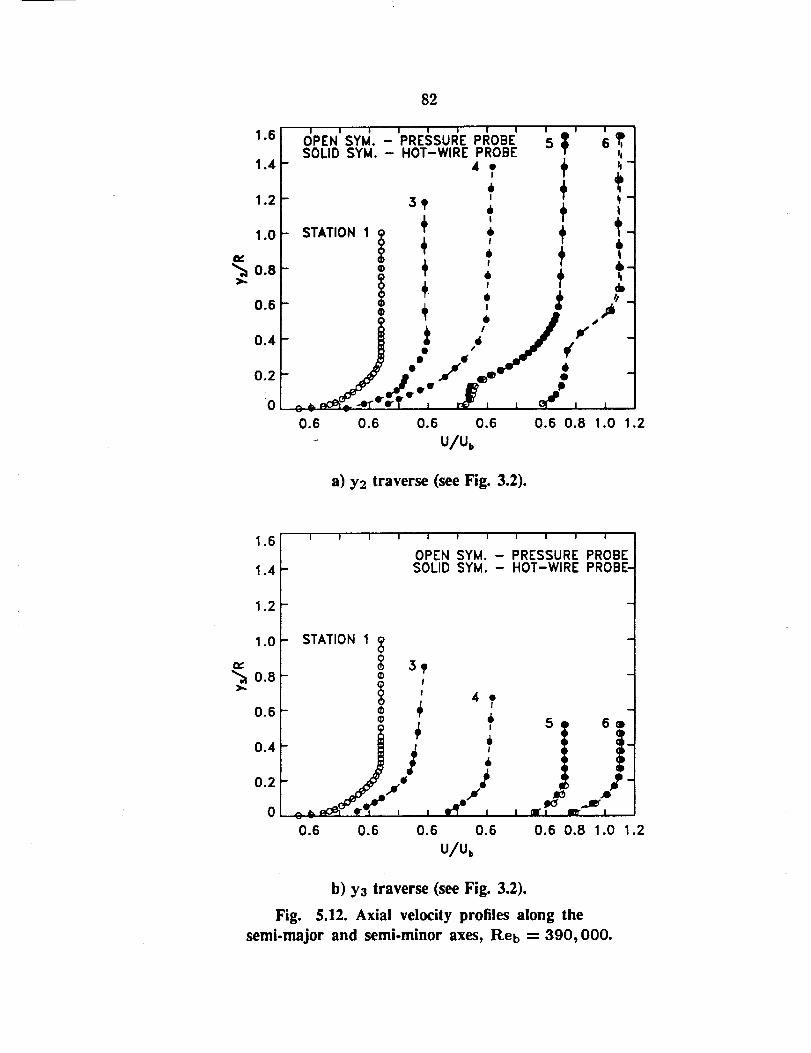
82
I I I I I ''I I I I I I
_.6 OPE.sYM.-PRESSUREPROBES:_ S_,SOLID SYM. - HOT-WIRE PROBE 'l1.4- , . _ ,,-
1.2- - i • i-
- STATION IQ + ; _ _-
1.0 _ _' i _ _'
0.8- _ + . + ,,-¢ ,i, I l cb9 T , ,i, ,,
0.6- _ .L i • ._, -
'l' • ,@" j
!
0.2 /o_0 _
0.6 0.6 0.6 0.6 0.6 0.8 1.0 1.2
u/u,,
a) y2 traverse (see Fig. 3.2).
1,6 I !
1.4
1.2
! I I I I I I I I
OPEN SYM. - PRESSURE PROBESOLID SYM. - HOT-WIRE PROBE-
1.0 STATION 1 _
'i0.6 -
°'I B ! ; ! |/o. F /.. } /I
o ¢_',,,a _0.6 0.6 0.6 0.6 0.6 O.B 1.0 1.2
u/u,
b) y3 traverse (see Fig. 3.2).
Fig. 5.12. Axial velocity profiles along the
semi-major and semi-minor axes, It.eb = 390,000.
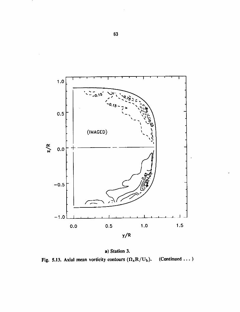
83
1.0
0.5
ev,
0.0N
-0.5
-1.0
-+
I ' ' ' ' I .... I '
- - _ = \It I'i_
i h
(IMAGED) .. ,.,,i1
I'"
l ' ' i l l , , , , l '
0.0 0.5 1.0
y/R
w , = I
I I 1
a) Station 3.
Fig. 5.13. Axial mean vorticity contours (f_xR/Ub). (Continued ... )
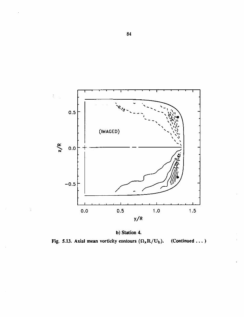
84
0.5
-0.5
-+
i' ' _ I .... I .... I
"o._ ..., _ _ ." -.
--, ,,_]l_l 1
(IMAGED) "- ',,'_
I ..... I _ , , _ I _ , , , I
0.0 0.5 1.0 1.5
y/R
b) Station 4.
Fig. 5.13. Axial mean vorticity contours (f_xR/Ub). (Continued ... )

85
rv,
N+
0.0 0.5
y/R
1.0 1.5
c) Station 5.
r_
N+
Fig.
O
0.0 0.5 1.0 1.5
y/R
d) Station 6.
5.13. Axial mean vorticity contours (f_xl:L/Ub).

iv
N
0.6
0.4
0.2
0.0
-0.2
-0.4
-0.6
86
-- 7-
¢,-j
fp
_f
Ilr"
)//,_ ,%,
I
0.5 1.0 1.5
y/R
a) Station 5.
r_
N
Fig.
I I
b) Station 6.
5.14. Axial turbulence intensity contours (u'/U x 102).

ef
N
0.6
0.4
0.2
0.0
-0.2
-0.4
-0.6
0.0
87
0.5
y/R
a) Station 5.
1.0 1.5
r_
N
0.6
0.4
0.2
0.0
-0.2
-0.4
-0.6
÷
• • • |
!
0.0
Fig.
, 1 , a : J I
0.5 1.0
y/R
b) Station 6.
S.lS. _/U_ × 10 4 Reynolds stress contours.
• I
1.5
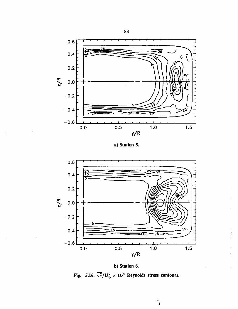
88
0.0N
0.5
y/R
a) Station 5.
1.0
r_
N0.0 +
0.0 0.5 1.0 1.5
y/R
b) Station 6.
Fig. 5.16. _'2/U_ x 104 Reynolds stress contours.
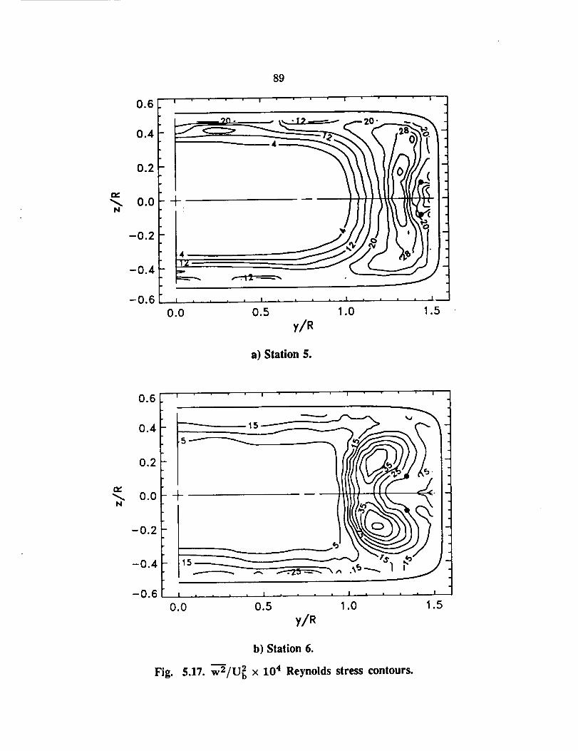
89
.6 I " " "' I I I .
0.2 ( i
o.o + ....... _I-:
-0.4
-0.6 , , , , .... ,
0.0 0.5 1.0 1.5
y/R
a) Station 5.
0.6
0.4
0.2
0.0N
-0.2
-0.4
-0.6
I I I I
15 -_-_._ _
%,/
J
[ • ,t • ! i I | I | , I I I I I
0.0 0.5 1.0 1.5
y/R
b) Station 6.
Fig. 5.17. _'3/U_ x 10 4 Reynolds stress contours.
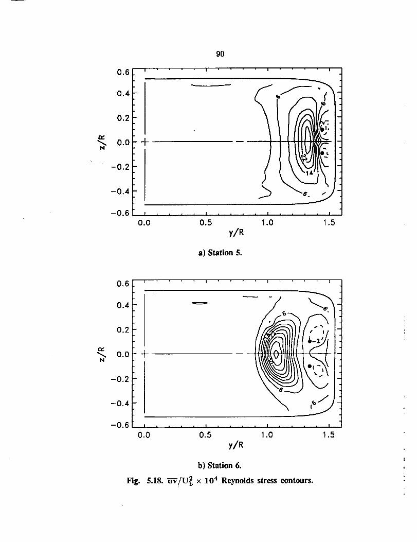
tv
N
0,6
0,4
0.2
0.0
-0.2
-0.4
-0.6
+
9O
f
I .... I • , _ • I .... I
0.0 0.5 1.0 1.5
y/R
a) Station 5.
{E
N
0.6
0.4
0.2
0.0
-0.2
-0.4
-0.6
I ' I I I
+
I • r 1 , . I I I J =_ J 1 ' ' .l • I
0.0 0.5 1.0 1.5
y/R
b) Station 6.
Fig. 5.18. h-v/U_) x 10 4 Reynolds stress contours.
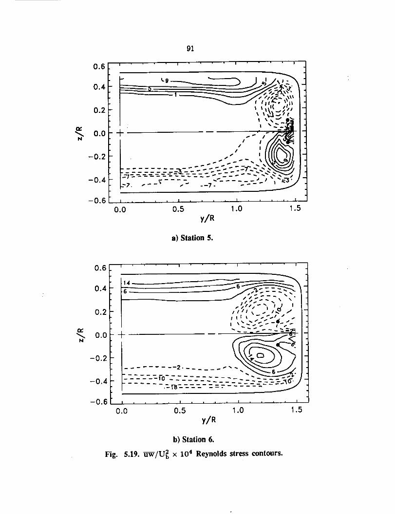
iv,
N
0.6
0.0
-0.2
-0.4
-0.6
91
I • I I
+
L
_ _,l _ ._,J I-_ _'N_ I
_"7. ,. _ _T - - - -._" ---7"
/s I /lJ !
J
I .... , I , • . _ I , . . = I
0.0 0.5 1.0 1.5
y/R
a) Station 5.
0.0 0.5 1.0 1.5
y/R
b) Station 6.
Fig. 5.19. _--_/U_ x 10 4 Reynolds stress contours.
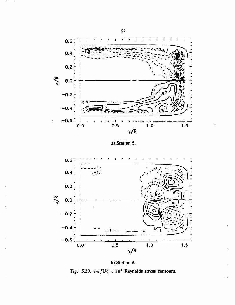
92
,6 I ' _ • • I I I
I "-- "x x J IfY'/9"= II "_ ,, -... -_qi';Zl.,--I
•. , ".,;!IUI,_I
l Jo-o.4 to..
"- -0.6 _ , , . . , .... , .... ,
0.0 0.5 1.0 1.5
y/R
a) Station 5.
O_
N
0.6
0.4
0.2
0.0
-0.2
-0.4
-0.6
I I I I
+
Fig.
.,m-_
I I ! i i I i I i i | I i i " I
0.0 0.5 1.0 1.5
y/R
b) Station 6.
5.20. V_/U_ x 10 4 Reynolds stress contours.
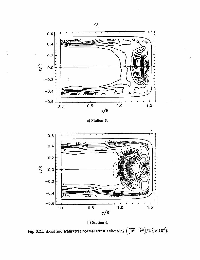
N
0.6
0.4
0.2
0.0
-0.2
-0.4
-0.6
I
÷
I
0.0
93
I ! !
• . . m I . . _. I o . 1
0.5 1.0 1.5
y/R
a) Station 5.
rw"
N
0.6
0.4
0.2
0.0
-0.2
-0.4
-0.6
I I I I
|
I-f
[ • . I . • • . I . . , • I
0.0 0.5 1.0 1.5
y/R
b) Station 6.
Fig. 5.21. Axial and transverse normal stress anisotropy /(u -_ - v2/ x 1041 .
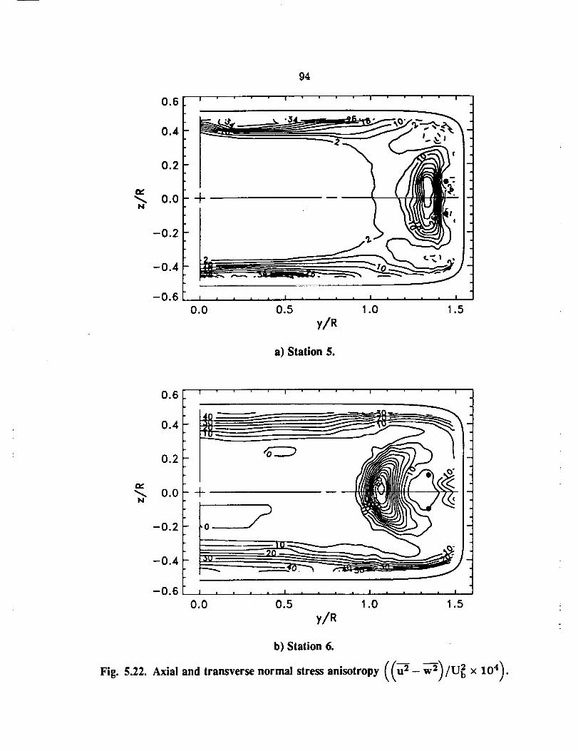
e=..
N
0.6
0.4
0.2
0.0
-0.2
-0.4
-0.6
r 1
94
I I I
I... _ j
m
I _ i i i I .... I .... I
0.0 0.5 1.0 1.5
y/R
a) Station 5.
!
*6 I I I I
0.4 _ -0.2
oo-0.2 i
-o.4 -
--0.6 1 , , , , I i ]
0.0 0.5 1.0 1.5
y/R °
b) Station 6.
Fig. 5.22. Axial and transverse normal stress anisotropy ((u-2- w-"_'l./U2x104).
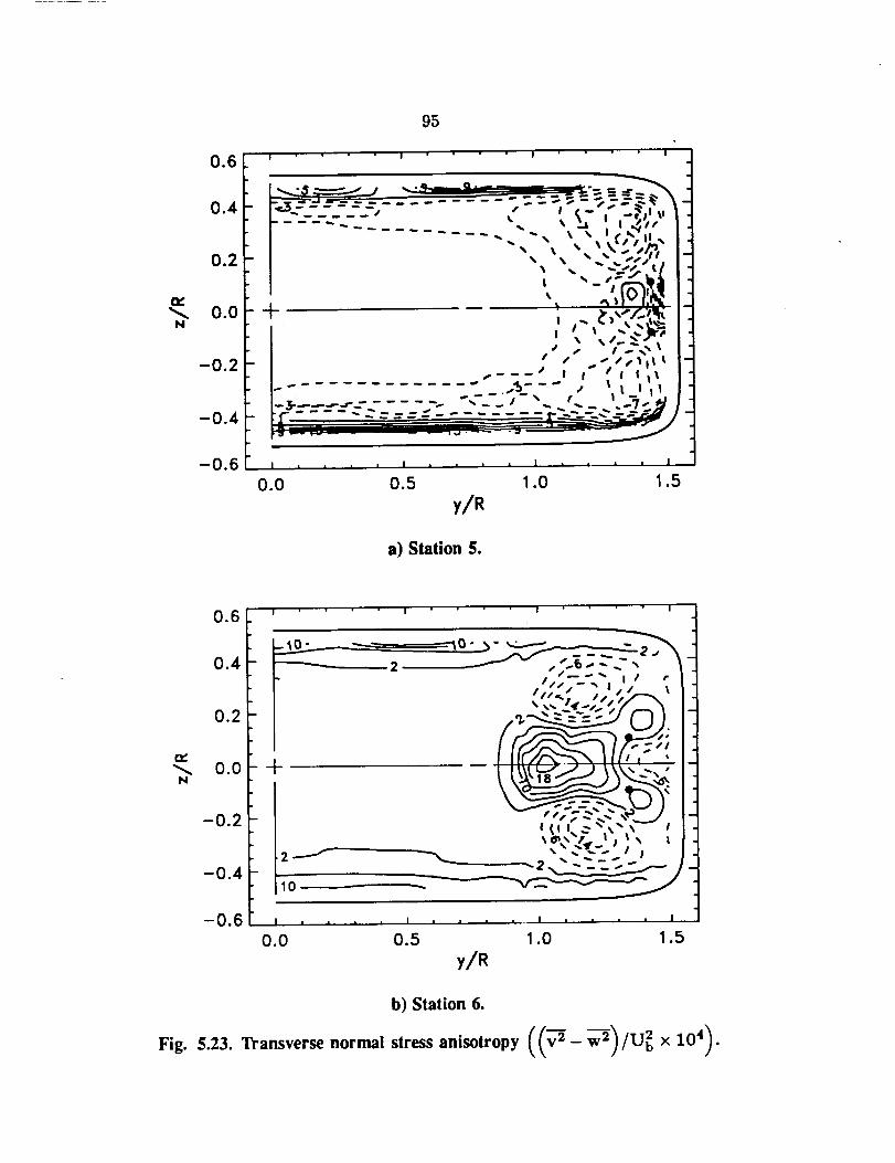
95
,6 I I I I
I",_ _--*'J ,,,.._- 9 ..... ___-.-- .__-_"_
0.4. ,,_ - -"
_- ..... - "-., ,_ ,;.-.'?.",.I• .. _...-_-_f 11
0.0 -1- • ,","_/.-".',_I' ,"." __.',_'_ I
i I " " ." .,.. Jlre I
'% - I-- _ "'." I
-o.2 ; " .-;',"',-t','I_'------ I ' "l _ I
--0.4 " -- = = = ........ " --_'_" _--.....-0.6 I • , , ' .......
0.0 0.5 1.0 1.5
y/R
a) Station 5.
0.6
0,4
0.2
rv-0.0
N
-0.2
-0.4
-0.6
I I I I
- _ ,, 2 -_ _ ,, _..f_ .. --.-_" xI /_'" I I r
i1_//-- • | i i
- ,_..._._-__-=-.j { } J
• jr. I I1[//'_'_\ illl _ "
2 J"
10
xx_.,.%. / i
| i • • . I i i i a I l • I
0.0 0.5 1.0 1.5
y/R
b) Station 6.
Fig. 5.23. "transverse normal stress anisotropy ((v-2 - w-2)/U_xl04).
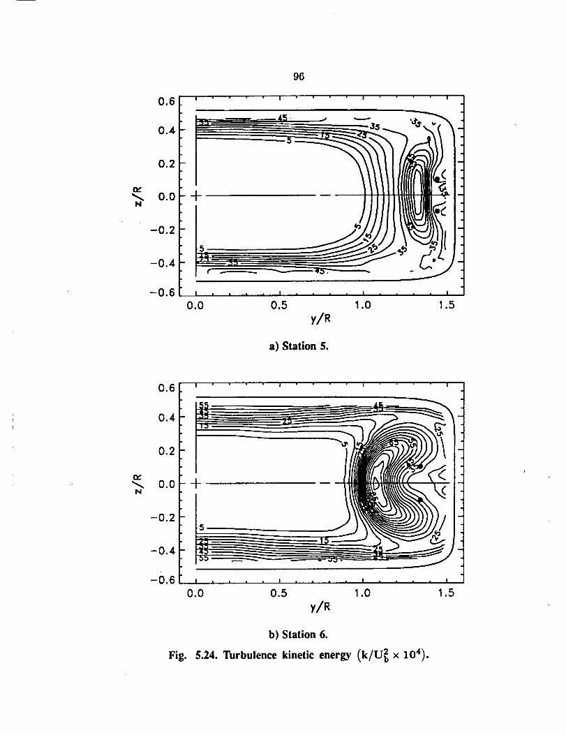
¢v
N
0.6
0.4
0.2
0.0
-0.2
-0.4
-0.6
96
I " " I " ' ' I
+
I J L .... L, * I • • !
0.0 0.5 1.0
y/R
a) Station 5.
rw
N
0.6
0.4
0.2
0.0
-0.2
-0.4
-0.6
r-- • _ • ' ' I ' ' I
I i | | | I | | ..IL. | I I " " "
0.0 0.5 I .0
y/m
Fig.
b) Station 6.
5.24. Turbulence kinetic energy (k/U_ x 104).
I
1.5
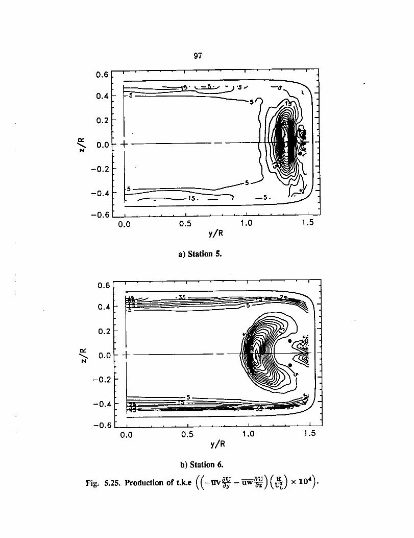
97
ew
N
0.0 0.5
y/R
a) Station 5.
c_
N+
-0.2
-0.4
-0.60.0 0.5 1.0
y/R
b) Station 6.
_aU _aUFig. 5.25. Production of t.k.e ((-uv_-- uw-_-) (_b)
× 104_ •
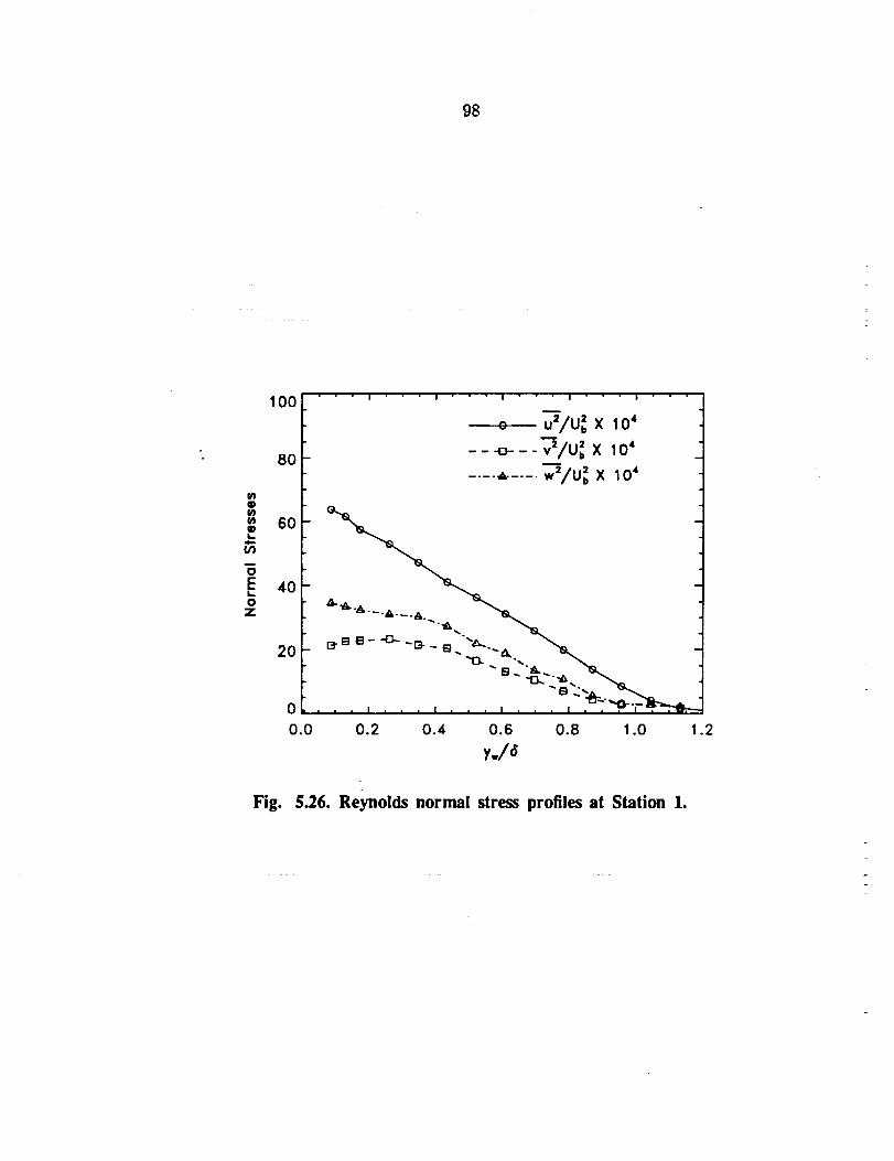
98
@
@
0
EI,,,,0
Z
100
8O
6O
4O
2O
0
o.o
I I I I I
o _/u: x,o'-- _---T%: x lO'.... --.... w'/u:x lo'
[3" [] B - _ -I_- - L-., ''_'._
-,_- _-.:__._,,._B ""_--o-
• • , I i J , I , • i I z z l I • I I "l" , , _,
0.2 0.4. 0.6 0.8 1.0 1.2
y./6
Fig. 5.26. Reynolds normal stress profiles at Station 1.

99
lOOL ' ' " " ' , , , • • .
= _/u: x ,0'80 - - -o----_/u; x lo'
i 60 ,, ...._/u:x_o,_ 40 ,,Z
0.0 0.2 0.4 0.6 0.8 1.0 .2
y_'6
a) Station 5.
1oo
b) Station 6.
Fig. 5.27. Normal stress profiles along semi-major axis at Stations 5 and 6.
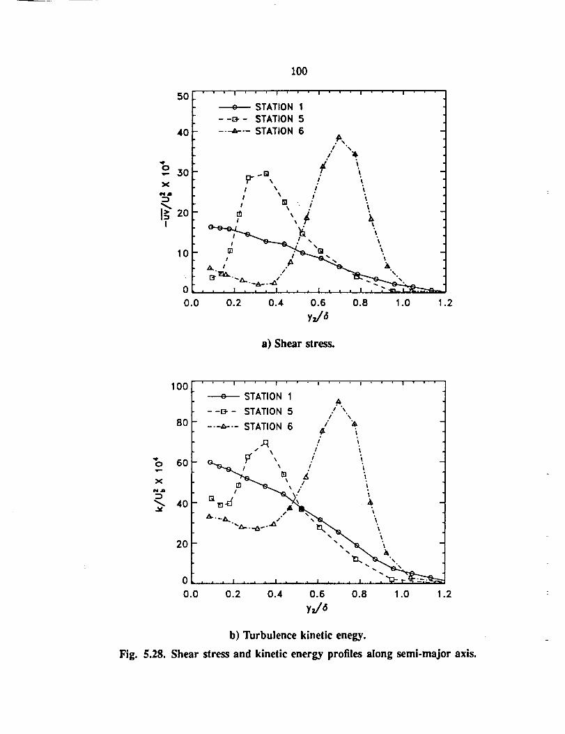
S0- • "
4O
o.- 30x
NJ
I._20I
10
0
0.0
100
• I ' * ' I
STATION I
--B-- STATION 5
---_-- STATION 6
_lgp- ,I
I _'i fil
I I I
'li i
i "_i "l
I °
I _ _.
_,, ".,
_.._. .,- _ il
0.2 0.4 0.6 0.8 1.0 .2
y=/6
a) Shear stress.
100
8O
_:_ 60
_ 40
20
0
0.0
I I I I
STATION 1,.-.,
--B-- STATION 5 /
----z,-.- STATION 6 4_.R / 'l
/ I t
._ ,/ "1
' 'l
_"-_,. ./" ',"6L"'_'"_i-"_ _,"'nt. '
. ,0.2 0.4 0.6 0.8 1.0
y=/6
.2
b) Turbulence kinetic enegy.
Fig. 5.28. Shear stress and kinetic energy profiles along semi.major axis.
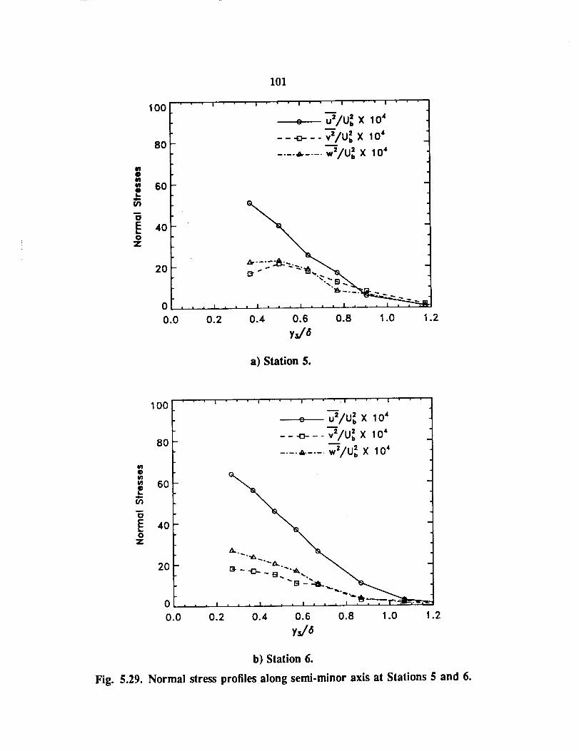
101
100
8O
= 60
2O
0
0.0
' ' ' ! ' " " I|'''1",,|,,,
- : Z/o: x ,o,---o-- _'/u: x lo'.... ,_.... w=/ub=x lO'
--<s ..\
• i _ I • i • I i | | _ = i =
0.2 0.4 0.6 0.8 1.0
y=/6.2
a) Station 5.
6'1
@
u_
-I,-,o'1
oEL
oZ
100
80
6O
4O
2O
0
0,0 0.2 0.4 0.6 0.8 1.0 1.2yJ6
b) Station 6.
Fig. 5.29. Normal stress profiles along semi-minor axis at Stations 5 and 6.
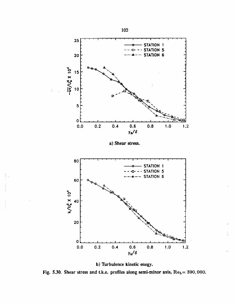
25
20
_r
0•- 15X
N.IJ
I-_ 10I
5
" ' I
102
I I I I
o STATION 1- - -o- - - STATION 5
.... _ .... STATION 6
0
0.0
% '%"% '%%
J_ • , i _ • • I , • _ I
0.2 0.4, 0.6 0.8 1.0
),J6
a) Shear stress.
.2
,q.
ow,,-
x
8O
6O
4O
2O
0
0.0
t I I I I
o STATION 1- - -0- - - STATION 5
.... •_..... STATION 6
%"%,
0.2 0.,4. 0.6 0.8 1.0
yJ6
.2
b) Turbulence kinetic enegy.
Fig. 5.30. Shear stress and t.k.e, profiles along semi-minor axis, Reb= 390,000.
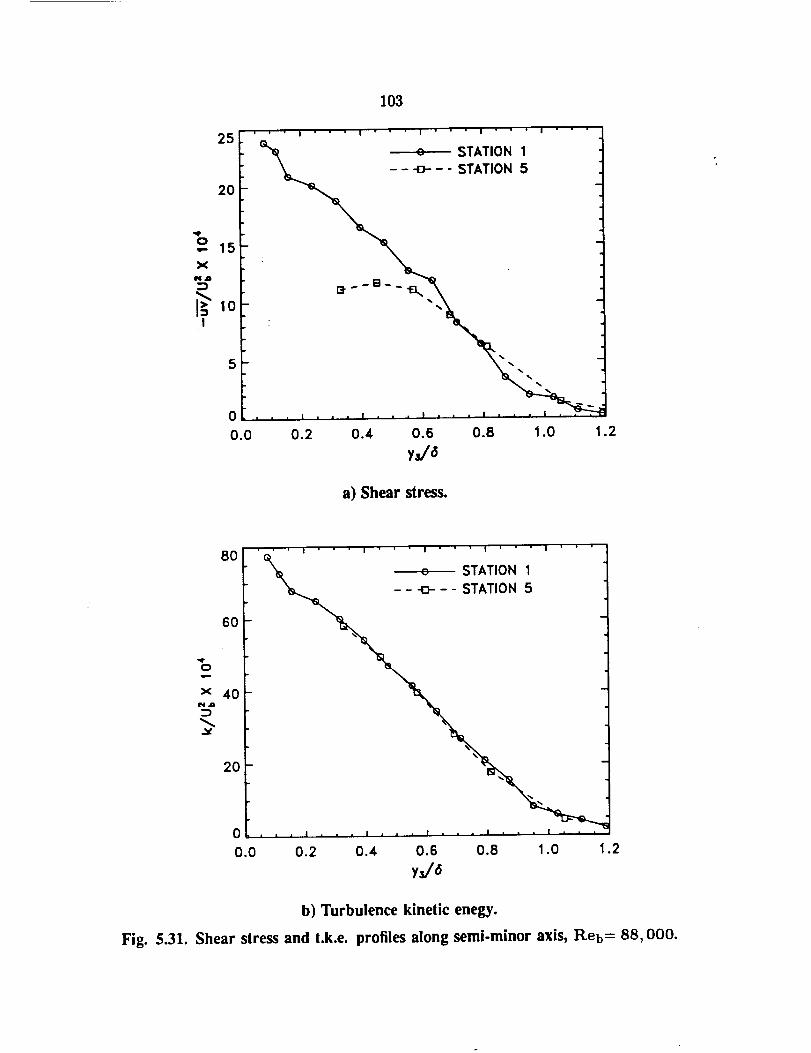
25
20
'ql'
o•- 15x
N_e,
I
5
0
0.0
103
I I I ' " " I I
.__ STATION 1STATION 5
%
I , • m I , | = • • • _ • '
0.2 0.4 0.6 0.8 1.0 1.2
yJ6
a) Shear stress.
8o
6o
x 40N,O
.=Y
2O
0
0.0
' ' ' I ' " ' I ' ' " I I I
o STATION 1
, ! , • • I • , , I = = , I • • , |
0.2 0.4 0.6 0.8 1.0 .2
yJ6
b) Turbulence kinetic enegy.
Fig. 5.31. Shear stress and t.k.e, profiles along semi-minor axis, Reb= 88,000.
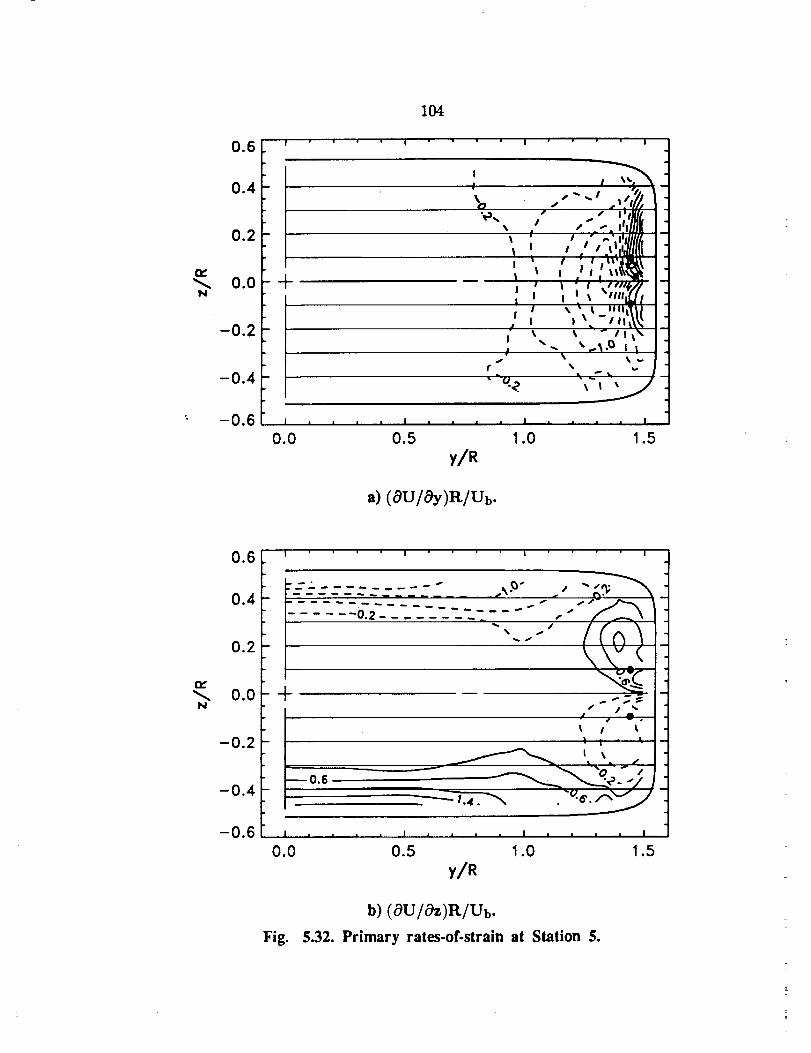
N
0.6
0.4
0.2
0.0
-0.2
-0.4
-0.6
+
I
0.0
I
I
%I
I
..--' .,,;//,. i I',JJll
/ ,:,. _.'. mljfllK
, t • u.u,a_
' I !1 ,/','._//I I I _ fill IrJ{
t ,,"k I "l|l(t|
| I
!
P
I
Js
i I,*, I I • • I
0.5 1.0 1.5
y/R
a) (aU/0y)R/Ub.
tv"
N
0.6
0.4
0.2
0,0
-0.2
-0.4
-0.6
I I I I
:..--- _- - _ _ __ _ _ - - _._- , -..,._ -_
+p
Sr / - .
k I k
--0.6
l • • • • J i l i • I • • , • J
0.0 0.5 1.0 1.5
Fig. 5.32.
y/R
b) (0U/cgz)R/Ub.
Primary rales-of-strain at Station 5.
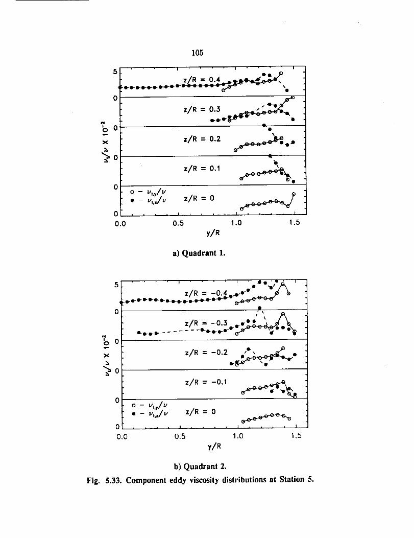
0
105
0
z/R = O. 1
• v,,,/v z/R = 0
0
0.0
y/R
a) Quadrant 1.
5
Fig.
O"
z/R = -0.1
0
0
0.00.5 1.0 1.5
y/R
b) Quadrant 2.
5.33. Component eddy viscosity distributions at Station 5.
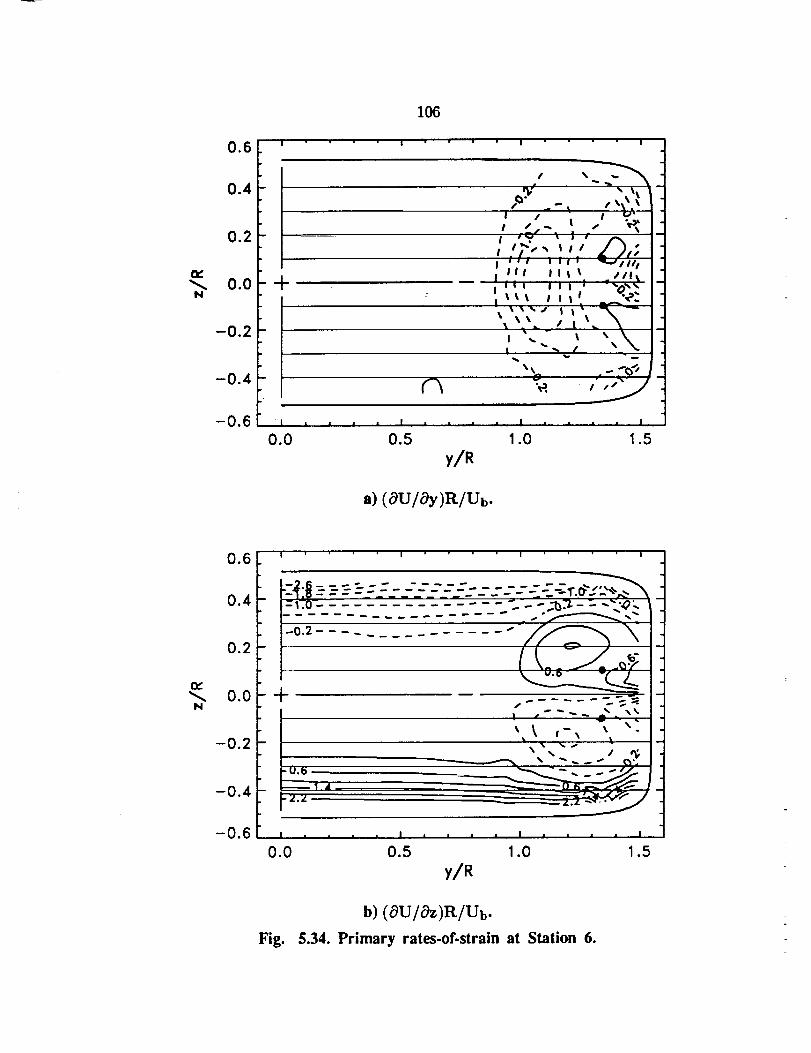
rv,
N
0.6
0.4
0.2
0.0
-0.2
-0.4
-0.6
106
I ! " " "
4- E
• I !
| / "
| 4,',,,, • ; •
l • • e i I I ' "_,,Jlll II _III_ I I I _. .III'*
i i t I I I I ' -"(_,_:)_l I_ I II I
"_' . - _0 "_ i _
| • • • • I • • •
0.0 0.5
y/R1.0 1.5
a) (aU/ogy)R/Ub.
N
0.6
0.4
0.2
0.0
-0.2
-0.4
-0.6 .... ] I ' • • I I , , , , I
0.0 0.5 1.0 1.5
y/R
b) (OU/Oz)R/Ub.
Fig. 5.34. Primary rates-of-strain at Station 6.
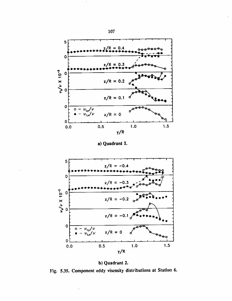
5
0
0
0
0.0
107
! I " •! --
z R=0.4
z/R = 0.!
y/R
a) Quadrant 1.
Fig.
5
_4!o 0
X z/R = -0.2 •0•0
0
0.0
y/R
b) Quadrant 2.
5.35. Component eddy viscosity distributions at Station 6.
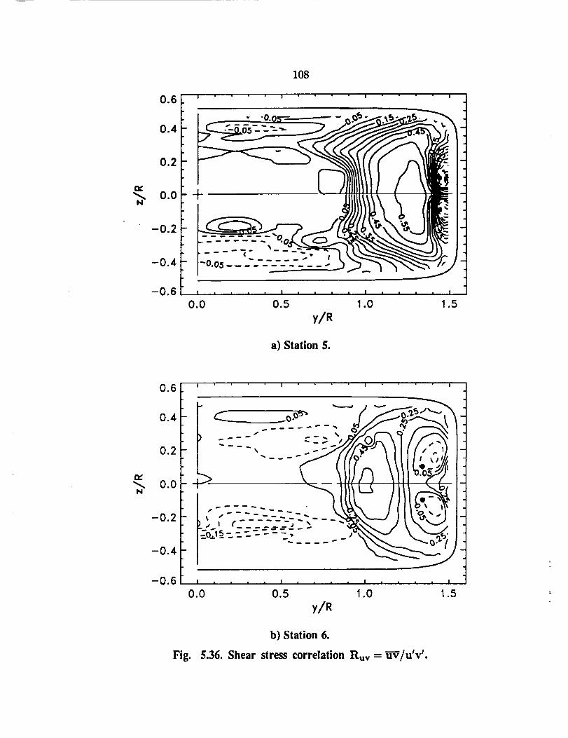
ew
N
0.6
0.4
0.2
0.0
-0.2
-0.4
-0.6
108
0.0 0.5 1.0 1.5
y/R
a) Station 5.
0.6
0.4
0.2
_,, 0.0N
-0.2
-0.4
-0.6
I I I I
| I i l i | i i i l i I I I i ]
0.0 0.5 1.0 1.5
y/R
b) Station 6.
Fig. 5.36. Shear stress correlation Ray = h-V/u'v'.
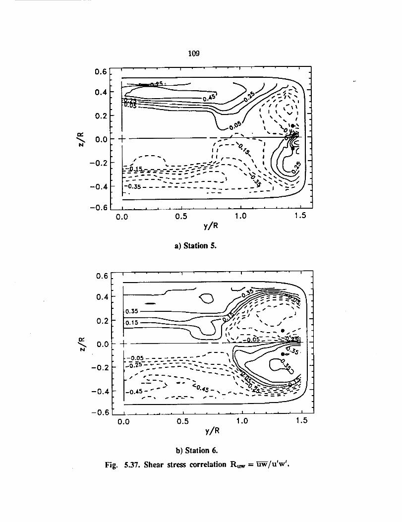
rv"
N
0.6
0.4
0.2
0.0
-0.2
-0.4
-0.6
109
I ! !
t, "<t i �J-T("----" I i t--. _ | I / f"
...... ----- _- _ .., -, " :, _";-,_/,
I I , , , • ]
0.0 0.5 1.0 1.5
x/R
a) Station 5.
.6 I I ' I I
0.2 -- o._5 _ _"-,Y,;" "-. _ J I-I
I" - _ _ ,-_'_-o.o5.-- -_.'_ I-1_ o.o_-_1 ,,, .... ----, "_' J_
-o.2 _ -._
F I-o.4s- - _ .4s.._ .. _ --.__=%_--;:- / -1
-0.6- , . , , • , .... , .... ' "0.0 0.5 1.0 1.5
y/R
b) Station 6.
Fig. 5.37. Shear stress correlation P,.uw = _-W/u'w'.
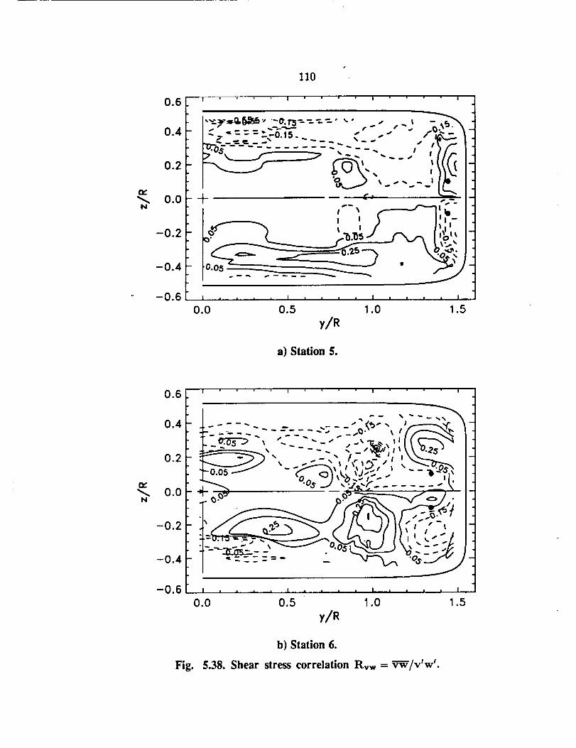
0.6
0.4
02
"_, 0.0N
-0.2
-0.4
-0.6
110
I I I I
,_Q.r_ v -o./-5-----_---, ,.- .., ,. i
,_--_-_,
l I III
i .... I , , , , I , • .j • I
0.0 0.5 1.0 1.5
y/R
a) Station 5.
N
0.6
0.0
-0.2
-0.4
-0.6
I ' ' " " l " ' ' ' I " ' " " I
_ ___.....I_o:'_-) _ .. "-" ,-,'.'v_._ ".1_ ___'_'_..... . ":._-:.-.'., ._._." ,:_.
"1--........_._.,,j , --_._- ,.:_,.r ,! _._
- ::_ _._,__-'_-.,_,:
J i • • • 1 _ , * • 1 • • , • [ ]
0.0 0.5 1.0 1.5
y/R
b) Station 6.
Fig. 5.38. Shear stress correlation Rvw = _/v'w'.
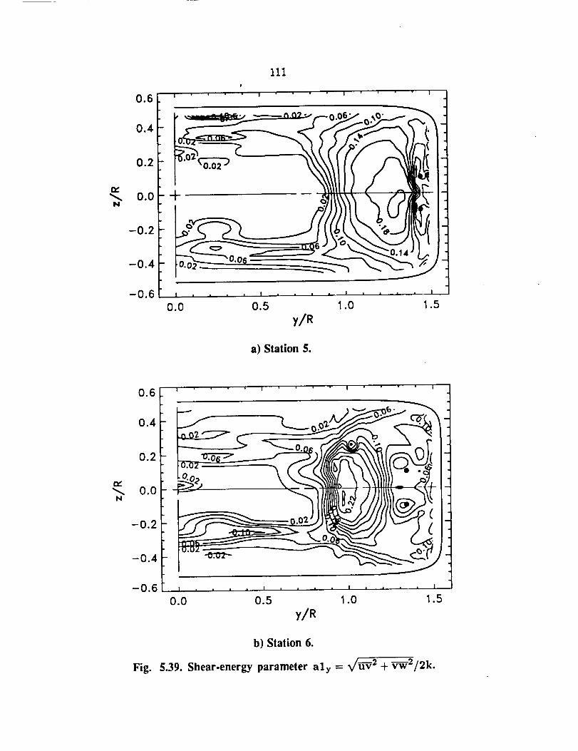
111p
0,6 J. I a I • ' I
-0.2 i
-0.4
-0.6
0
y/R
a) Station 5.
0.6
0.4
0.2
n.,"_ 0.0N
-0.2
-0.4
-0.6
| " I ' = • g
. 1 = I I
10.0 0.5 1.0 1.5
y/R
b) Station 6.
Fig. 5.39. Shear-energy parameter aly = _/h-V 2 -t-Vw2/2k.
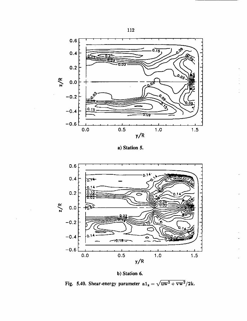
112
0.6_ ' ' ' ' 1
01 10.2
o.o_0.0
-0.2
-0.4
-0.6
0.0 0.5 1.0 1.5
y/R
a) Station 5.
,6 t I I I-4
,.4
0.2 " _ .---- ._
_'N 0.0
-0.2
-0.4
-0.6 | = I • • = a • • • • • [
0.0 0.5 1.0 1.5
y/R
b) Station 6.
Fig. 5.40. Shear-energy parameter alz = _/_-W2 + Vw2/2k.
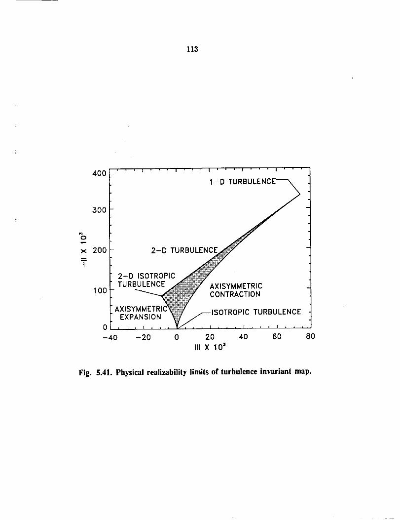
113
0
X
I
400
300
200
100
1-D TURBUI.
2-D TURBULENCE
2-D ISOTROPICTURBULENCE
AXISYMMETRI(EXPANSION
0
-40 -20
AXISYMMETRICCONTRACTION
,TROPIC TURBULENCE
0 20 40 60 80
III X 105
Fig. 5.41. Physical realizability limits of turbulence invariant map.
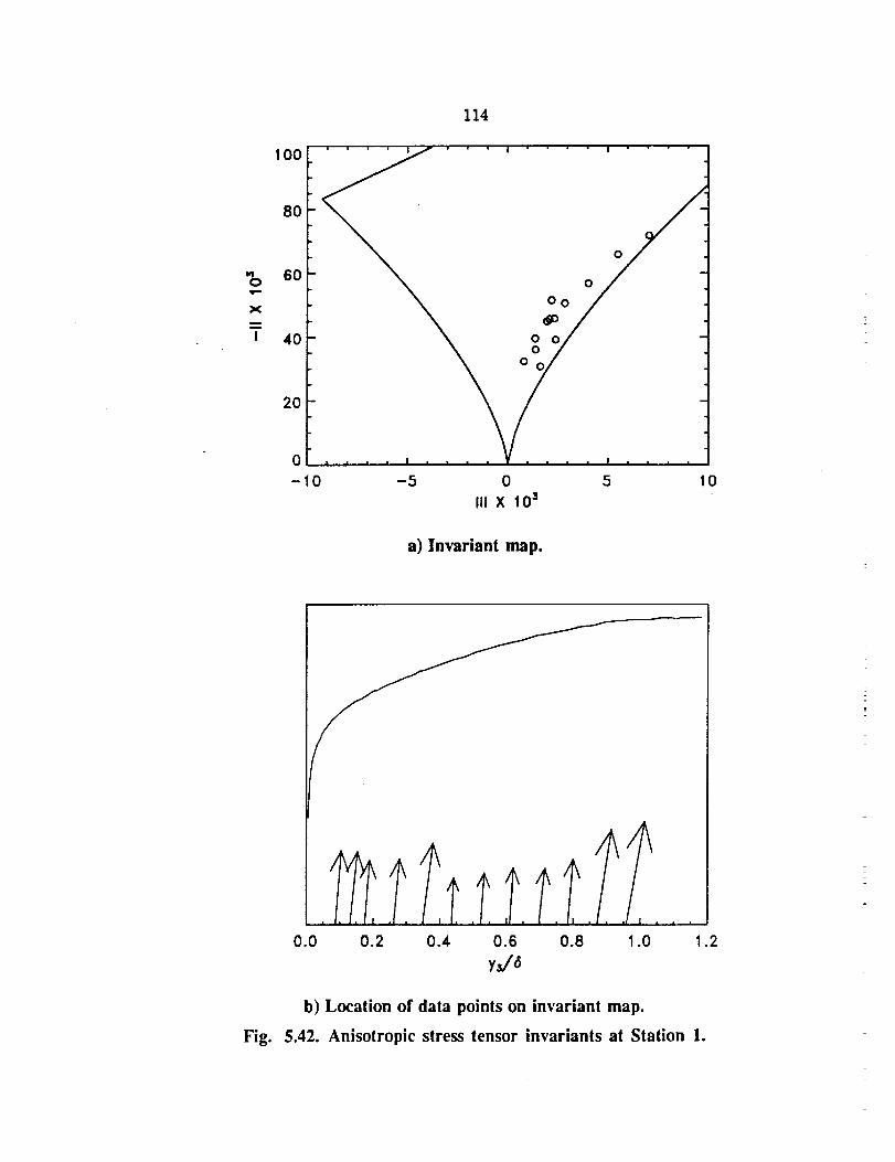
100
114
8O
I@
0
X
I
6O
4O
O0
0 00
0
0
2O
0
-10 -5 0 5
III X 10 s
10
a) Invariant map.
Fig.
0.0
] • • i
.0 1.2
b) Location of data points on invariant map.
5.42. Anisotropic stress tensor invariants at Station 1.
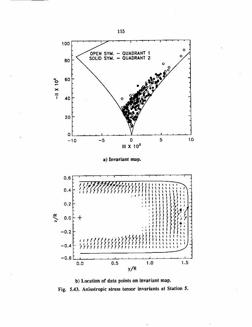
115
0
X
I
1O0
8O
6O
4O
20
0
-10
OPEN SYk'I. - QUADRANT 1SOLID SYk'I. - QUADRANT 2
-5 O
III X 10 3
0o
5
0
0
10
a) Invariant map.
r,"
N
0.6
0.4
0.2
0.0
-0.2
-0.4
-0.6
Fig.
I ! I
.etttJ I, t
+
. I
o I
// /t//ftltttt
ttltlilttt_t_lit|ttltaltt.Ill.itt,ttt.ttf,ttt_tftJl|t
ttt_It !tI I I I
. I
% _
tttt tt it
, /tt _
k I t
I _ , _ . I = . . , I . , • • l
0.0 0.5 1.0 1.5
y/R
b) Location of data points on invariant map.
5.43. Anisotropic stress tensor invariants at Station 5.
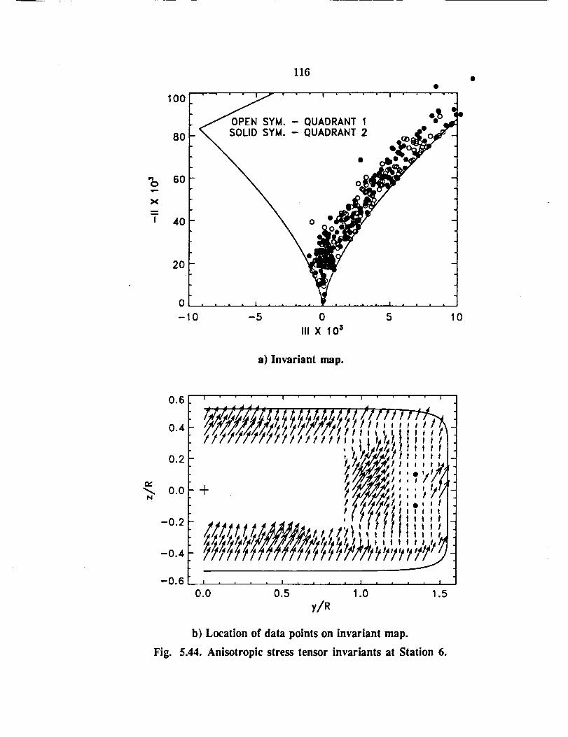
116
I@
0
X
I
100
8O
6O
4O
2O
0
-10
OPEN SYk4. - QUADRANT 1SOLID SYM. - QUADRANT 2
0
0
-5 0 5
III X 10 5
10
a) Invariant map.
N
0.6
0.4
0.2
0.0
-0.2
-0.4
-0.6
Fig.
I I I
7_J_M,'/,'£Zf,f,/,t,f,f,t,l,f,/,1,f.ffl ! /
, t '/#P,_/t t,,,,,,,, t/ I/I/f'fJ(_/ t'-""-'-" , o _ t g_
"/_1. , . , ,77;/_/;,r_.1,
''[ [ It t'''t, , ()*f ttttt
//777777 7"/77 '/'/7'/'/
).0 0.5 1.0 1.5
_/R
b) Location of data points on invariant map.
5.44. Anisotropic stress tensor invariants at Station 6.
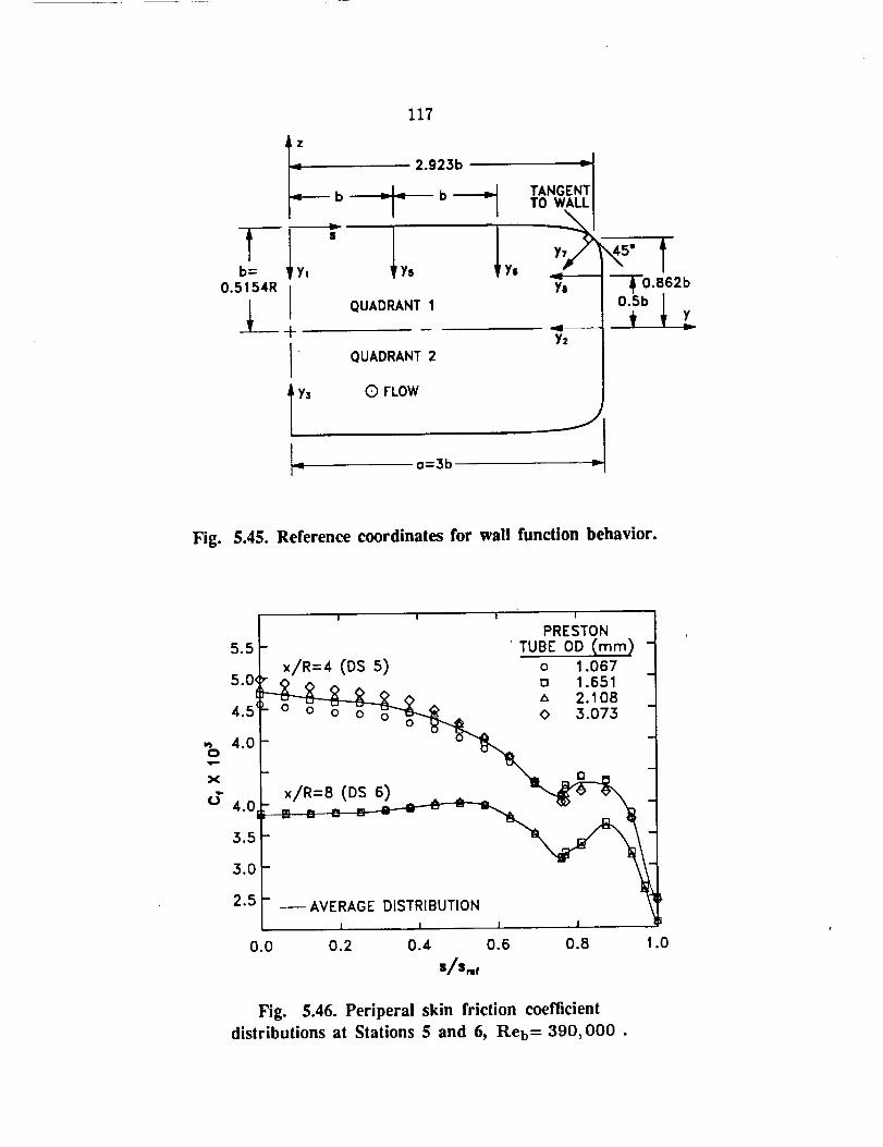
b=0.5154R
1_
117
z
_---- b
Y!
$
2.923b TANGENT[
-- b-_ 1 TO WALLI
Y8QUADRANT 1
-t'- -- Y2QUADRANT 2
l y_ E) FLOW
L 0=3bV" _1
--To.862b
0.5bt Y
Fig. 5.45. Reference coordinates for wall function behavior.
' ' ' PRESTON5.51- "TUBE OO (ram) -
/ x/R=4 (DS 5) o 1.06750<_" ,-,• _ v o ^ _ [] 1.651 -
P--_--A--2LW <> ^ z_ 2.108
4.5L o _ _ 0 3.073 -o 15,,,_
- ("1 _
x - x/R=8 (DS 6) . _I_
o 4.0_
3.5-
3.0
2.5 - __ AVERAGE DISTRIBUTION
I I I I
).0 0.2 0.4 0.6 0.8
S/Smf
Fig. 5.46. Periperal skin friction coefficient
distributions at Stations 5 and 6, Reb= 390,000 .
.0
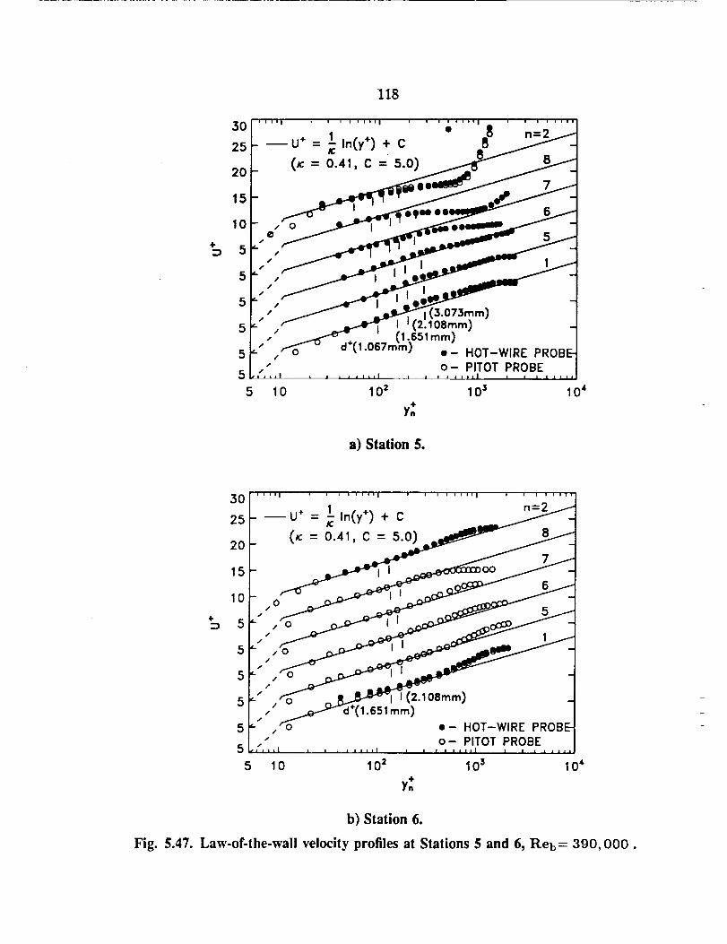
4"
30
25
20
15
10
5
5
5
5
5
5
5
118
1 in(y+) + C--U÷ = E-
10 102 103 104
y.+
a) Station 5.
3o
25
20
15
10
5
5
5
5
5
5
I I I I I _ I I , I I , I I ! I I I , I I I | I ! i i i i i i
- --o"--_,o(,')÷c __
7_ _
L/f/
_-'/ 0 _ _2"_, OBtain)
,, _-/ d+(1.651 ram)
, o e- HOT-WIRE PROBE" o- PITOT PROBE
i#J I [ II l l I J ] I I iI l I I I l I J J I l I I i z i i i
10 102 103 04
b) Station 6.
Fig. 5.47. Law-of-the-wall velocity profiles at Stations 5 and 6, Reb= 390,000.
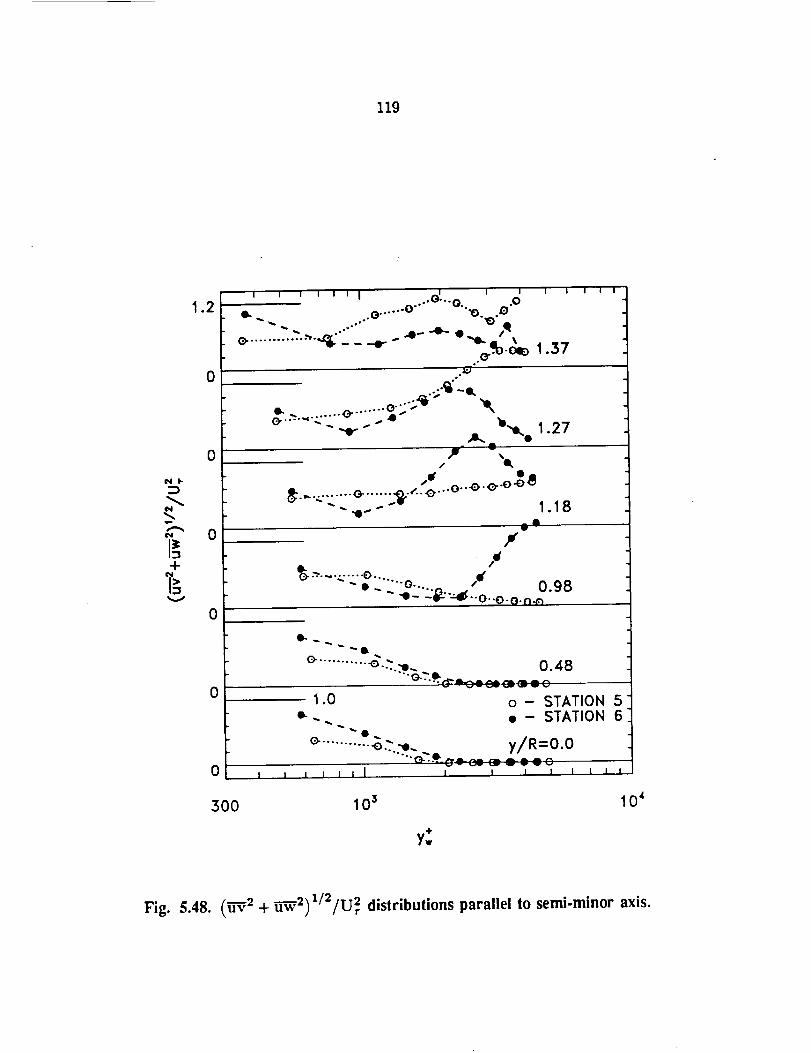
119
N l-
e.N
+
V
1.2
0
0
0
0
0
0
I I I I I I J _I I I I I I I I
...... O-'- 0 .O0.._ O...... O" "'_B. __,D
.._r.-:o.o_ 1.37D
i •
w
Y.... " 0.98
-o- '"_" "'-¢: "'O-.o.o. n _
e. ........... -o ..':.:_ ,, .. 0.48c""o.-.._. _Lc.e__ _,._m _ _
1.0 o- STATION 5"--... • - STATION 6
...... _-.e-_ :'..-e.... y/R=O.O.... O'"O"-CL_ _ _ ¢ ¢ O
I I l I I I l I I I I i t t
300 10 _ 10 4
y:
Fig. 5.48. (h-V 2 + _-W 2) 1/2/U2, distributions parallel to semi-minor axis.
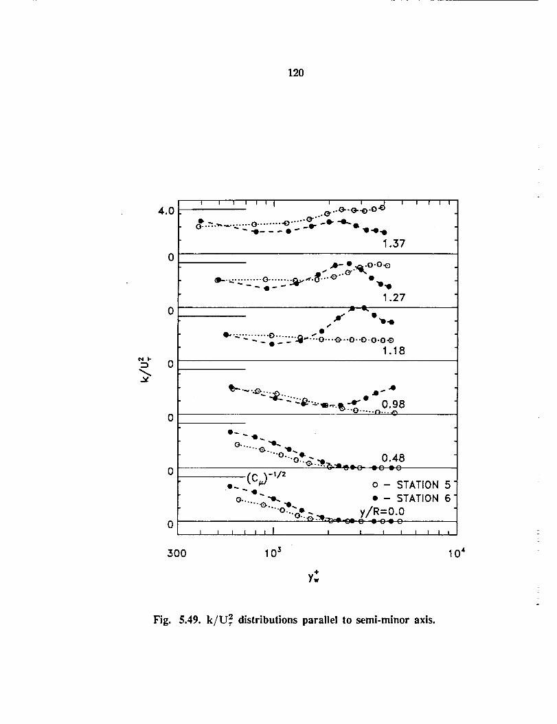
120
e41-
4.0
0
0
0
0
0
0
.•- • _t.O-O_
m-" _.._'_<1_............ 0 ....... -Q,_,<-iS".'" •
1.27,_-&.
f . "D.e
_ _ • - _ :._ ""O'-'_)'--O--O-O-O.Q1.18
-"+ "'_--o ..... n.0.._ 8
O_
.... ,Q..... 01--11,.... 0.48
0.._..._.._._.=,,,_ ¢0 ¢0
,... "--LC_-I/z o- STATION 5
e..... "_ •- STATION 6
"'°"- o.°.S ..._:_.. Y/R_ 0-O
J ] | n | J ] t [ i I I i I
300 1 03 104
y:
Fig. 5.49. k/U_ distributions parallel to semi-minor axis.
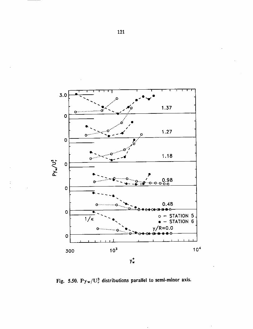
121
l@ I-
3.0
0
0
0
n
0
0
0
I I I I I I ii
"%
"% .0.'%"%
% ,,,"
"% .• ."
I ! I I I I I I
,af'_ 1.37S ,,
..¢_ •
oO°
" >..,:...e" ..o" o 1.27O" ..... "%0 _ _ o,
_.')
0.,,. ..... .0 .... "'" Ie- ...... _- ,, ,. __6 1.18
o.. ,o
e- ...... -.,.-B,-,-.o ..... o- -' 0.98-o- -o- "-;41_"o-.o-o.o.e
...._
...........o.
o- STATION 51/_; ".
" • - STATION 6%
" y/R........... -e.. •- =0.0.....ek_"-e- _ _-------= _ o
I i i I I I I I I 1 1 I u I
300 10 _ 104
y:
Fig. 5.50. Pyw/U a, distributions parallel to semi-minor axis.
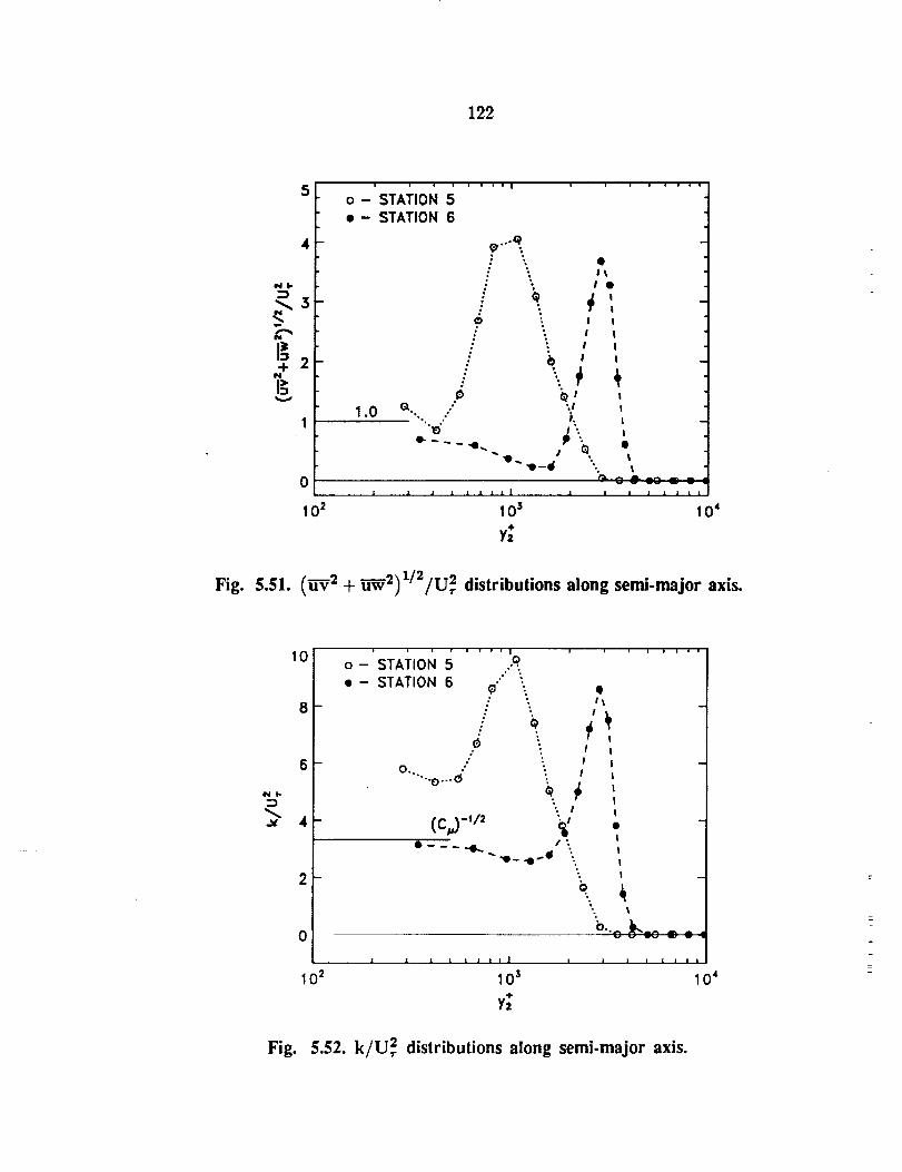
122
4
Z--
+ 2N
i>_
| | ! i i ! i ! |
o- STATION 5•- STATION 6
01 i i i I I 1 i |
102 10s
y;
_,*°°_
' I_
: "* I •
" ir z
I t: 6 I i
- ÷ _
1.0 _ ' :t I"'" J'. t• .. °,"
"" "0.,. l--d " II_-_ _-_ _, _
] i I I i i i i
04
Fig. 5.51. (h-V 2 + R'w'2)l/2/U2 distributions along semi-major axis.
¢qt-
10
8
6
2-
0
10 2
f . i i i i v i I
o- STATION 5 ..o..•- STATION 6 ."¢
0"--..0...i _"
¢
Q _; I
(c,,)-'/' i'• ------"O,. I :
" "0- .O _ "
1 I l n t l t | l i
103
y;
Q
I iI I
I i
i
I
I
I
I
•, !
" !
"_..o_:o = :.
| 1 1 1 1 I 1
10 4
Fig. 5.52. k/U_ distributions along semi-major axis.
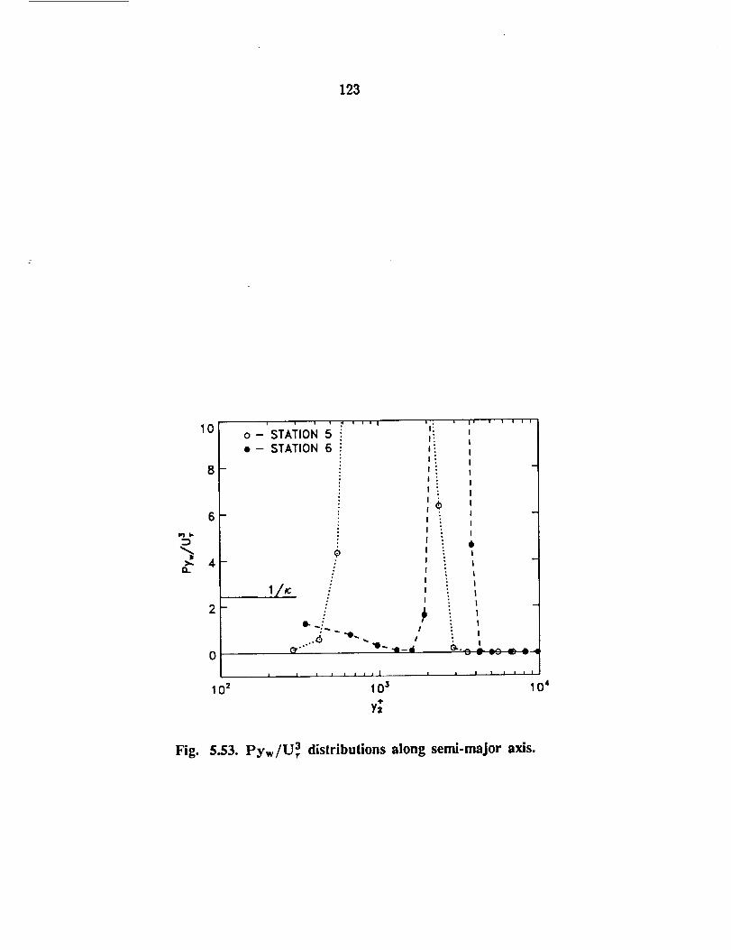
123
n
10
8-
6-
4-
2
0
02
o- STATION 5•- STATION 6
0
1/_
| I 1
I;J!J_
I
1_ .m_,¢
I L n I t ! I
103
y;
i
w wv
I I I i i t |
10 4
Fig. 5.53. Pyw/UT 3 distributions along semi-major axis.
CHAPTER6
CONCLUSIONS AND RECOMMENDATIONS
6.1 Conclusions
Incompressible, turbulent, swirl-freeflow through a circular-to-rectangular
transition duct has been studied experimentally. Mean flow measurements are
presented at fiveaxial stations and the complete Reynolds stresstensor ispre-
sented at three axialstationsfor operating bulk Reynolds numbers of 88,000 and
390,000. No significantReynolds number dependence was observed and excellent
symmetry prevailedthrough the entiretestsection.The resultsof the study may
be summarized as follows:
i)The inlet conditions to the duct, which correspond to partially developed
turbulent pipe flow, proved to be an interesting case, in itself, considering
the large differences between results of various studies on the subject. The
present results showed that the boundary layer was significantly thinner
than that reported by other investigators over nearly equivalent development
lengths (x/D ,,_ 9). Reynolds stress levels also differed. These discrepancies
are generally attributable to inlet conditions at the pipe entrance. Excellent
law-of-the-wall behavior was observed in the pipe and the skin friction was
very near the fully-developed value.
2) The results of the transition duct measurements show that streamwise vor-
ticity generated in the first half of transition strengthens and concentrates
along the duct sidewall in the second half of the transition resulting in a
contra-rotating vortex pair (common flow away from surface) centered about
the duct semi-major axis. The upwash action between the vortices creates
a region of low wall shear stress. The vortex pair significantly distorts the
mean flow and turbulence fields.
3) In the transition section, transverse flow velocities of approximately 32% of
the inlet bulk velocity were observed. In the constant area duct extension,
the vortex pair causes a secondary flow to persist that peaks at about 12%
of the inlet bulk velocity.
4) In the vicinity of the sidewall vortices, a large velocity deficit exists. The
large primary rates-of-strain associated with this velocity deficit dominate
much of the vortex region. These large strain rates produce a region of
relatively high turbulence intensity.
5) In the vicinity of the vortex cores, nearly isotropic turbulence exists which
is dramatically attenuated by lateral convergence effects.
IJMtlE /_.__IHTEHTiON ALLY BLANKPRECED;F-_G PA_E BLANK NOT FILMED
126
6) Along the horizontal walls at the end of transition, a peculiar trend in the
primary turbulent shear stress was observed which is a result of surface
curvature and lateral divergence effects. This anomaly was manifested in
a dramatic reduction in the shear stress midway across the boundary layer
as the wall is approached. The measurements did not, however, resolve the
near-wall region to determine if the shear stress recovered in the inner layer.
7) At the end of transition, law-of-the-wall behavior indicates that the flow is
in local equilibrium over only a very small regio n near the wall. Trends inturbulence-based wall function behavior at this station tend to support the
local equilibrium assumption, but the present measurements do not fully
resolve the near-wall region. At the end of the transition duct extension,
local equilibrium is observed over a fairly large region near the wall.
The present results can serve as an experimental database for CFD code calibra-
tion/yerification, inasmuch as the results demonstrate the appropriate symmetry
and are based on well-defined inlet conditions. The results of this study should
also provide a stringent test for turbulence models. To facilitate comparisons,
the transition duct geometric variables are available in Appendix A. Tabulated
flow data in machine readable form are available from the author.
6.2 Recommendations
Between the time that the present study was initiated and completed, a
number of studies dealing with circular-to-rectangular transition ducts appeared
in the literature. Most notable are those of Reichert et al. [4] and Miau et aI.
[9]. Despite these additions, there are still some areas which have not been fully
addressed. First among these is the case with inlet swirl. Inlet swirl may be
beneficial from the standpoint of reduced noise and thermal plume. Although
Reichert has provided mean flow data at several axial stations in a CR transition
duct, a large region in the vicinity of the sidewall was not accessible. Supplemen-
tary mean flow data in this region and turbulence measurements in the entire
cross-plane will provide a more complete picture for the swirling case. Another
area of interest is the case of laminar flow through a CR transition duct. This
is of interest because laminar flow data are useful for code validation purposes.
Having both laminar and turbulent data allows the code developer to distinguish
between deficiencies in the numerical scheme and in the turbulence model. Fi-
nally, measurements in a different geometry transition duct may be useful. In
particular, investigation of an identical duct to the one used in the present study,
but without the area variation, may give further insight to the development of
streamwise vortices, inasmuch as it has been observed that ducts which have
no area expansion are devoid of vortices. Discrete vortices have been observed,
however, in ducts which have an area expansion, for different aspect ratios and
transition lengths. All of the above research extensions could be made in the
127
present facility with minimal hardware change. The swirling case requires only
the addition of turning vanes in the inlet pipe or, preferably, a swirl generator
similar to the one proposed by Reichert which very nearly approximates a solid-
body rotation inlet condition. For the laminar flow case, in addition to removing
the boundary layer trip, a means for reducing the flow rate through the facility
would be required to ensure that the flow remained laminar through the entire
test section. This could be accomplished by providing a controllable bypass flow
downstream of the test section.

REFERENCES
1) Stevens, H.L., Thayer, E.B., and Fullerton, J.F., "Development of the Multi-
Function 2-D/C-D Nozzle," AIAA Paper 81-1491, 1981.
2) Patrick, W.P., and McCormick, D.C., "Circular-to-Rectangular Duct Flows:
A Benchmark Experimental Study," SAE Technical Paper 871776, 1987.
3) Patrick, W.P., and McCormick, D.C., "Laser Velocimeter and Total Pres-
sure Measurements in Circular-to-Rectangular Transition Ducts," Report
No. 87-41, United Technology Research Center, East Hartford CT, June
1988.
4) Reichert, B.A., Hingst, W.R. and Okiishi, T.H., "An Experimental Compar-
ison of Nonswirling and Swirling Flow in a Circular-to-Rectangular Transi-
tion Duct," AIAA Paper 91-0342, 1991.
5) Mayer, E., "Effect of Transition in Cross-Sectional Shape on the Develop-
ment of the Velocity and Pressure Distribution of the Turbulent Flow in
Pipes," NACA TM903, 1939.
6) Taylor, A.M.K.P., Whitelaw, J.H., and Yianneskis, M., "Turbulent Flow in
a Square-to-Round Transition," NASA Contractor Report CR-3447, July,
1981.
7)
8)
9)
10)
11)
12)
Burley II, J.R., and Carlson, J.R., "Circular-to-Rectangular Transition
Ducts for High-Aspect Ratio Nonaxisymmetric Nozzles," AIAA Paper 85-
1346, 1985.
Burley II, J.R., Bangert, L.S., and Carlson, J.R., "Investigation of Circular-
to-Rectangular Transition Ducts for High-Aspect Ratio Nonaxisymmetric
Nozzles," NASA Technical Paper TP-2534, March, 1986.
Miau, J.J., Leu, T.S., Chou, J.H., Lin, S.A. and Lin, C.K., "Flow Distortion
in a Circular-Rectangular Transition Duct," AIAA Journal, Vol.28, August
1990,pp.1447-1456.
Schwartz, I.R., "Minimization of Jet and Core Noise of a Turbojet Engine
by Swirling the Flow," AIAA Paper 75-503, 1975.
Beer, J.M., and Chigier, M.A., Combustion Aerodynamics, Applied Science
Publishers, London, 1972, pp. 100-146.
Der, J. Jr., Chu, C., Hunt, B.L. and Lorincz, D.J., "Evolution of Swirl in
a Two-Dimensional Nozzle Flow," Journal of Aircraft, Vol.19, April 1982,
pp.347-349.
PRECEDL{'_G PAGE BLAr_K NOT FILMED
130
13) Chu, C., Der, J.Jr. and Wun, W., "A Simple 2D Nozzle Plume for IR
Analysis," AIAA Paper 80-1808, Aug. 1980.
14) Chu, C. and Der, J.Jr., "Modelling of 2D Nozzle Plume for IR Signature
Predictions Under Static Conditions," AIAA Paper 80-1808, Aug. 1980.
15) Sobota, T.H., and Marble, F.E,, Swirling Flows in an Annular-to-Rectang-
ular Transition Section," Journal of Propulsion and Power, Vol.5, No.3,
May-June 1989, pp.334-340.
16) Vu, T.C. and Shyy, W., "Navier-Stokes Flow Analysis for Hydraulic Turbine
Draft Tubes," Journal of Fluids Engineering, Vol.12, June 1990,pp.199-204.
17) Bradshaw, P.,"Effects of Streamline Curvature on Turbulent Flow," AGAR-
Dograph 169, 1973.
18) So, R.M.C., and Mellor, G.L., "Experiment on Convex Curvature Effects in
Turbulent Boundary Layers," Journal of Fluid Mechanics, Vol.60, Part 1,
1973, pp. 43-62.
19) So, R.M.C., and Mellor, G.L., "Experiment on Turbulent Boundary Layers
on a Concave Wall," Aeronautical Quarterly, Vol.26, 1975, pp. 35-50.
20) Meroney, R.N., and Bradshaw, P., "Turbulent Boundary Layer Growth
over a Longitudinally Curved Surface," AIAA Journal, Vol.13, No.ll, 1975,
pp.1448-1453.
21) Hoffmann, P.H., Muck, K.C., and Bradshaw, P., "The Effect of Concave
Surface Curvature on Turbulent Boundary Layers," Journal o.f Fluid Me-
chanics, Vol.161, 1985, pp. 371-403.
22) Moser R.D., and Moin, P., "The Effects of Curvature in Wall-Bounded Tur-
bulent Flows," Journal of Fluid Mechanics, Vo1.175, 1987, pp. 479-510.
23) Gibson, M.M, "Effects of Surface Curvature on the Law-of-the-Wall," Near-
Wall Turbulence, Hemisphere Pub. Corp., New York, 1990, pp.157-171.
24) Hoffmann, P.H., and Bradshaw, P., "Turbulent Boundary Layers on Surfaces
of Mild Longitudinal Curvature," Imperial College Aeronautics Report, 78-
04, 1978.
25) Gillis, J.C., and Johnston, J.P., "Turbulent Boundary Layer Flow and Struc-
ture on a Convex Wall and its Redevelopment on a Flat Wall," Journal of
Fluid Mechanics, Vol.135, 1983, pp. 123-153.
26) Smits, A.J., Young, S.T.B, and Bradshaw, P., "The Effect of Short Regions
of High Surface Curvature on Turbulent Boundary Layers," Journal of Fluid
Mechanics, Vol.94, Part 2, 1979, pp. 209-242.
131
27) Hunt, I.A., and Joubert, P.N., "Effects of Small Streamline Curvature on
Turbulent Duct Flow," Journal of Fluid Mechanics, Vol.91, Part 4, 1979,
pp. 633-659.
28) Muck, K.C., Hoffmann, P.H., and Bradshaw, P., "The Effect of Convex Sur-
face Curvature on Turbulent Boundary Layers," Journal of Fluid Mechanics,
Voi.161, 1985, pp. 347-369.
29) Shabaka, I.M.M:A, Mehta, R.D. and Bradshaw, P., "Longitudinal Vortices
Imbedded in Turbulent Boundary Layers. Part 1. Single Vortex," Journal
of Fluid Mechanics, Vo1.155, 1985, pp.37-57.
30) Mehta, R.D. and Bradshaw, P., "Longitudinal Vortices Imbedded in Turbu-
lent Boundary Layers. Part 2. Vortex Pair with 'Common Flow' Upwards,"
Journal of Fluid Mechanics, Voi.188, 1988, pp.529-546.
31) Pauley, W.R. and Eaton, 3.K., "The Fluid Dynamics and Heat Transfer
Effects of Streamwise Vortices Embedded in a Turbulent Boundary Layer,"
Standford University Thermosciences Report MD-51, 1988.
32) Pauley, W.R. and Eaton, J.K., "Boundary Layer Turbulence Structure in
the Presence of Embedded Streamwise Vortices," Seventh Symposium on
Turbulent Shear Flows, Stanford University, 1989.
33) Liandrat, J., Aupoix, B and Cousteix, "Calculation of Longitudinal Vor-
tices Imbedded in a Turbulent Boundary Layer," Turbulent 3hear Flows 5,
Springer-Verlag, 1987, pp.253-258.
34) Bradshaw, P., "Turbulent Secondary Flows", Annual Review of Fluid Me-
chanics, Vo1.19, 1987, pp.53-74.
35) Bansod, P. and Bradshaw, P., "The Flow in S-Shaped Ducts," Aeronautical
Quarterly, Vol.23, Part 2, 1972, pp.131-140.
36) Taylor, A.M.K.P., Whitelae, J.H. and Yianneskis, M., "Developing Flow in
S-Shaped Ducts, Part II - Circular Cross Section Duct," NASA CR 3759,Feb. 1984.
37)
3s)
39)
Smits, A.J., Eaton, J.A., and Bradshaw, P., "The Response of a Turbulent
Boundary Layer to Lateral Divergence," Journal of Fluid Mechanics, Vol.94,
Part 2, 1979, pp. 243-268.
Morel, T., " Comprehensive Design of Axisymmetric Wind Tunnel Contrac-
tions," Journal of Fluids Engineering, Vol.97, June 1975, pp.225-233.
Towne, C.E. and Hoffman, J.D, "Computation of Viscous Flow in Planar
and Axisymmetric Ducts by an Implicit Marching Procedure," NASA TM
83567 (also AIAA Paper 84-0256), 1984.
43)"
132
40) Eppich, H. M., "An Experimental Investigation of the Turbulence Struc-
ture in the Inner Region of a Three-Dimensional Streamwise Corner," M.S.
Thesis, Dept. of Mech. Eng., University of Washington, 1982.
41) Chue, S.H., "Pressure Probes for Fluid Measurments," Progre,s in Aerospace
Sciences, Vol. 16, No. 2, 1975, pp. 147-223.
42) Comte-Bellot, G., Strohl, A. and Alcaraz, E.,"On Aerodynamic Distur-
bances Caused by Single Hot-Wire Probes," Journal of Applied Mechanica,
Vol.38, 1971, pp. 767-774.
Head, M.R. and Vasanta Ram, V., "Simplified Presentation of Preston Tube
Calibration," AeronauiicaI Quarterly, Vol. 22, Part 3, 1971, pp. 295-300.
44) Patel, V.C., "Calibration of the Preston Tube and Limitations on it's Use
in Pressure Gradients," Journal of Fluid Mechanics, Vol. 23, 1965, pp. 185-
208.
45) A1-Beirutty, M. H., "Development of a Hot-Wire Measurement Technique for
Moderate Intensity Three-Dimensional Flows," Ph.D. Dissertation, Dept. of
Mech. Eng., University of Washington, 1987.
46) A1-Beirutty, M. H., Arterberry, S.H., and Gessner, F.B., "A Hot-Wire Tech-
nique for Complex Turbulent Flows," Proe. of the 1st National Fluid Dy-
namics Congress, Part 3, AIAA Publications, New York, 1988, pp 1479-1486.
47) Arterberry, S. H., "An Improved Method of Flow Field Determination in
Three-Dimensional Flows of Low Intensity and Moderate Skewness," M.S.
Thesis, Dept. of Mech. Eng., University of Washington, 1982.
48) Klein, A., " REVIEW: Turbulent Developing Pipe Flow," Journal of Fluids
Engineering, Vol.103, June 1981, pp.243-249.
49) Barbin, A.R and Jones, J.B.,"Turbulent Flow in the Inlet Region of a
Smooth Pipe," Journal of Basic Bngingeering, Vol.85, No.l, March 1963,
pp.29-39.
50) Richman, J.W. and Azad, R.S.,"Developing Turbulent Flow in a Smooth
Pipe," Applied Scientific Research, Vol.28, 1973, pp. 419-441.
51) Reichert, J.K. and Azad, R.S.,"Nonasymptotic Behavior of Developing Tur-
bulent Pipe Flow," Canadian Journal of Physics, Vol.54, 1976, pp. 268-278.
52) Martinuzzi, R., and Pollard, A.,"Comparative Study of Turbulence Models
in Predicting Turbulent Pipe Flow, Part I: Algebraic Stress and k-e Models,"
AIAA Journal, Vol.27, Jan. 1989, pp. 29-36.
53) Pollard, A. and Martinuzzi, R.,"Comparative Study of Turbulence Models in
Predicting Turbulent Pipe Flow, Part Ih Reynolds Stress and k-e Models,"
AIAA Journal, Vol.27, Dec. 1989, pp. 1714-1721.
133
54) Schlichting, H., Boundary-Layer Theory, 7th ed., McGraw-Hill, New York,
1979, pp.565-566.
55) Fritsch, F.N. and Carlson, R.E., "Piecewise Cubic Interpolation Methods,"
Lawerence Livermore Laboratory Report No. UCRL-81230, November, 1978.
56) Bradshaw, P, Ferris, D.H. and AtweU, N.P., "Calculation of Boundary Layer
Development Using the Turbulent Energy Equation," Journal of Fluid Me-
chanics, Vol.28, 1967, pp.593-616.
57) Lumley, J.L. and Newman, G.R, "The Return to Isotropy of Homogeneous
Turbulence," Journal o.[ Fluid Mechanic._, Vol.82, Part 1, 1977, pp.161-178.
58) Rotta, J.C. "Statistische theorie nichthomogener turbulenz," Mitteilung-
Zeitschrift ffir Physik, Vol. 129, 1951, pp.547-572.
59) Gessner, F.B., Eppich, H.M. and Lurid, E.G., "The Near-Wall Structure of
Turbulent Flow Along a Streamwise Corner," Proc. of the 8th Symposium
on Turbulent Shear Flows, Munich, Germany, Sept. 1991.
60) Beyer, W.H.ed., CRC Standard Mathematical Tables, 25th ed., CRC Press
Inc., 1978.
61) De Grande, G. and Kool, P., "An Improved Experimental Method to Deter-
mine the Complete Reynolds Stress Tensor with a Single Rotating Slanting
Wire," Journal of Physics, Part E, Vol.14, 1981, pp.196-201.
62) Page, R. J., "An Experimental Study of Developing Turbulent Flow in a
Square Duct," M.S. Thesis, Dept. of Mech. Eng., University of Washington,1971.
63) Friehe, C.A, and Schwarz, W.H., "Deviations from the the Cosine Law for
Yawed Cylindrical Anemometer Sensors," Journal of Applied Mechanics,
Vol.35, No.4, Dec. 1968, pp.655-662.
64) Lawn, C.J., "The Determination of the Rate of Dissipation in Turbulent
Pipe Flow," Journal of Fluid Mechanics, Vol.48, Part 3, 1971, pp.477-505.
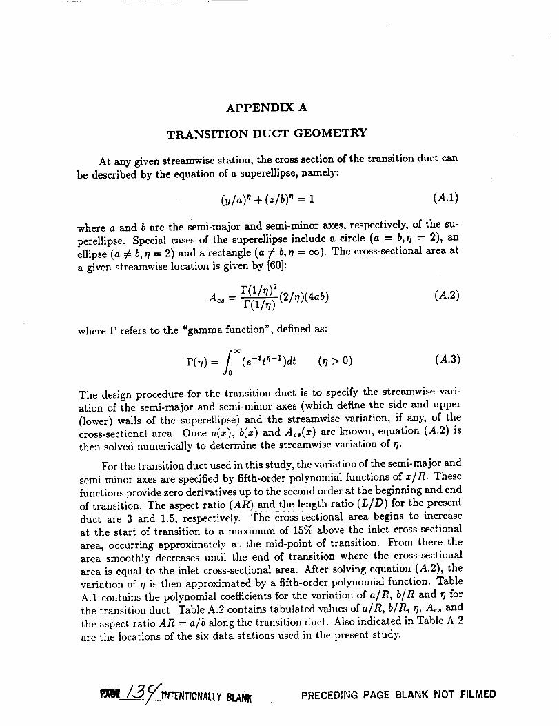
APPENDIX A
TRANSITION DUCT GEOMETRY
At any given streamwise station, the cross section of the transition duct can
be described by the equation of a supereUipse, namely:
(vla). + (zlb) = 1 (A.1)
where a and b are the Semi-major and semi-minor axes, respectively, of the su-
perellipse. Special cases of the superellipse include a circle (a = b, r/ = 2), an
ellipse (a # b, 7/= 2) and a rectangle (a # b,r/= ¢¢). The cross-sectional area at
a given streamwise location is given by [60]:
Ac,- F(1/rI)2(21TI)(4ab) (A.2)
where F refers to the "gamma function", defined as:
_0 _= (e-tt¢-l)dt (77 > 0) (A.3)
The design procedure for the transition duct is to specify the streamwise vari-
ation of the semi-major and semi-minor axes (which define the side and upper
(lower) walls of the superellipse) and the streamwise variation, if any, of the
cross-sectional area. Once a(z), b(x) and Ac,(x) are known, equation (A.2) is
then solved numerically to determine the streamwise variation of _.
For the transition duct used in this study, the variation of the semi-major and
semi-minor axes are specified by fifth-order polynomial functions of x/R. These
functions provide zero derivatives up to the second order at the beginning and end
of transition. The aspect ratio (AR) and the length ratio (L/D) for the present
duct are 3 and 1.5, respectively. The cross-sectional area begins to increase
at the start of transition to a maximum of 15% above the inlet cross-sectional
area, occurring approximately at the mid-point of transition. From there the
area smoothly decreases until the end of transition where the cross-sectional
area is equal to the inlet cross-sectional area. After solving equation (A.2), the
variation of r/is then approximated by a fifth-order polynomial function. Table
A.1 contains the polynomial coefficients for the variation of a/R, b/R and t/for
the transition duct. Table A.2 contains tabulated values of a/R, b/R, rI, Ac, and
the aspect ratio AR = a/b along the transition duct. Also indicated in Table A.2
are the locations of the six data stations used in the present study.
PRECEDIL_G PAGE BLANK NOT FILMED
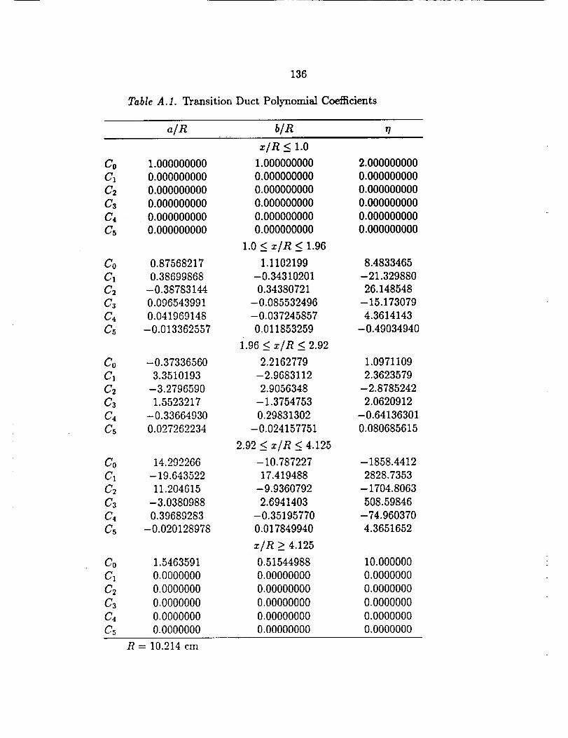
CoClCOCOC4CO
CoC1
COCOc4c5
CoCa
COCoc4Co
CoC1
Cz
CsC_CO
CoCa
Cz
C3C4C5
136
Table A. 1. Transition Duct Polynomial Coefficients
a/R b/R ,1
1.000000000
0.000000000
0.000000000
0.000000000
0.000000000
0.000000000
0.87568217
0.38699868
-0.38783144
0.096543991
0.041969148
-0.013362557
-0.37336560
3.3510193
-3.2796590
1.5523217
-0.33664930
0.027262234
14.292266
-19.643522
11.204615
-3.0380988
0.39689283
-0.020128978
1.5463591
0:0000000
0.0000000
0.0000000
0.0000000
0.0000000
xlR _ 1.0
1.000000000
0.000000000
0.000000000
0.000000000
0.000000000
0.000000000
1.0 _ z/R _ 1.96
1.1102199
-0.34310201
0.34380721
-0.085532496
-0.037245857
0.011853259
1.96 _ x/R_ 2.92
2.2162779
-2.9683112
2.9056348
-1.3754753
0.29831302
-0.024157751
2.92 < x/R _ 4.125
-10.787227
17.419488
-9.9360792
2.6941403
-0.35195770
0.017849940
z/R > 4.125
0.51544988
0.00000000
0.00000000
0.00000000
0.00000000
0.00000000
2.000000000
0.000000000
0.000000000
0.000000000
0.000000000
0.000000000
8.4833465
-21.329880
26.148548
-15.173079
4.3614143
-0.49034940
1.0971109
2.3623579
-2.8785242
2.0620912
-0.64136301
0.080685615
-1858.4412
2828.7353
-1704.8063
508.59846
-74.960370
4.3651652
10.000000
0.0000000
0.0000000
0.0000000
0.0000000
0.0000000
R = 10.214 cm
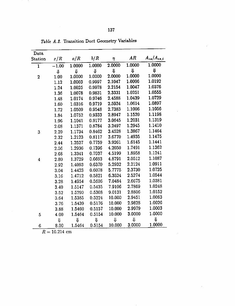
137
Table A._. Transition Duct Geometry Variables
Data
Station x/R air b/R _7 AR Ac,/Ac,.i
1 -1.00 1.0000 1.0000 2.0000 1.0000 1.0000
2 1.00 1.0000 1.0000 2.0000 1.0000 1.0000
1.12 1.0003 0.9997 2.1047 1.0006 1,0192
1.24 1.0025 0.9978 2.2154 1.0047 1.0376
1.36 1.0078 0.9831 2.3331 1.0251 1.0555
1.48 1.0174 0.9746 2.4588 1.0439 1.0729
1.60 1.0316 0.9719 2.5934 1.0614 1.0897
1.72 1.0509 0.9548 2.7383 1.1006 1.1056
1.84 1.0752 0.9333 2.8947 1.1520 1.1198
1.96 1.1041 0.9177 3.0645 1.2031 1.1319
2.08 1.1371 0.8784 3.2497 1.2945 1.1410
3 2.20 1.1734 0.8462 3.4528 1.3867 1.1464
2.32 1.2123 0.8117 3.6770 1.4935 1.1475
2.44 1.2527 0.7759 3.9261 1.6145 1.1441
2.56 1.2936 0.7396 4.2050 1.7491 1.1362
2.68 1.3341 0.7037 4.5199 1.8958 1.1241
4 2.80 1.3729 0.6693 4.879I 2.0512 1.1087
2.92 1.4093 0.6370 5.2932 2.2124 1.0911
3.04 1.4423 0.6078 5.7775 2.3730 1.0725
3.16 1.4712 0.5821 6.3524 2.5274 1.0544
3.28 1.4954 0.5606 7.0484 2.6675 1.0381
3.40 1.5147 0.5435 7.9106 2.7869 1.0248
3.52 1.5290 0.5308 9.0131 2.8806 1.0152
3.64 1.5385 0.5224 10.000 2.9451 1.0083
3.76 1.5439 0.5176 10.000 2.9828 1.0026
3.88 1.5460 0.5157 10.000 2.9979 1.0003
5 4.00 1.5464 0.5154 10.000 3.0000 1.0000
6 8.00 1.5464 0.5154 10.000 3.0000 1.0000
R - 10.214 cm

APPENDIX B
HOT-WIRE DATA ACQUISITION SYSTEM
An all new integrated hot-wire data acquisition system was acquired for the
present study. This system differs from previous ones used within the M.E.
department in that, rather than operating directly on the analog anemometer
output, data reduction operations are performed on a digital representation of
the analog signal. This appendix contains a description of the system and an
overview of some of the more important operating features.
B.1 Hardware
The primary components of the system are a Thermal Systems Incorporated
(TSI) IFA 100 Intelligent Flow Analyzer, a TSI IFA 200 analog-to-digital (A/D)
converter and a Digital Equipment Corporation (DEC) VAXLab/VSII Scientific
Workstation computer. A block schematic of this equipment is illustrated in Fig.
B.1.
The IFA 100 used in this study is a two-channel unit consisting of a Model
158 slave cabinet housing two Model 150 constant temperature anemometers and
two Model 157 signal conditioners. The signal conditioners contain a low-pass
filter, a high-pass filter and an amplifier capable of applying a DC offset (when the
high-pass filter is in the DC mode) and gain to the input (anemometer output)
signal. The usable range of the Model 158 digital display and the input voltage
range of the IFA200 digitizer is +5 volts. Most wire and film sensors will have
a voltage span much less than this. To utilize as much of this range as possible,
the transducer signal must be offset and amplified.
The IFA 200 provides high-speed simultaneous A/D conversions of one or
more anemometer output signals. Selectable A/D conversions rates of up to
50,000 Hz per channel provide the capacity of collecting data on rapidly changing
signals. The computer controls the IFA 200 by sending ASCII characters through
an RS-232 serial communication link. The parameters that are controlled through
this link are the starting address (channel to be sampled first), the number of
active channels and the sampling rate. For each sample, the A/D converter
generates a 16-bit data word. The low 12-bits contain the binary representation
of the transducer voltage. The high 4-bits contain the digitizer channel address
which must be stripped from the 16-bit data word before converting the binary
number to a hexadecimal voltage. The 16-bit data word is loaded into a 64-
word-deep first-in, first-out (FIFO) memory. The data that enter the FIFO pass
to the FIFO output and are sent via a DMA (Direct Memory Access) interface
cable to a DRQ3B DMA controller card in the computer.
P_I_/_'_ INTENTJONALLY_!1 PRECEDZNG PAGE BLANK NOT FILMED
140
The DRQ3B Parallel DMA I/O module is a high-speed memory interface
that allows real-time collection of 16-bit parallel digital data at transfer rates
of up to 1.3 megaHz. The DRQ3B has a unique feature, referred to as double
buffering, that can significantly increase data transfer rates as compared to con-
ventional single buffer DMA transfers. With single buffer DMA, when a buffer
fills, it is dequeued, but requires a software call to enqueue the next buffer. Dur-
ing the time between dequeueing the previous buffer and enqueueing the next
buffer, no data are transferred. This time between buffers must not exceed the
time it takes to fill the 64-word-deep FIFO memory in the IFA200, or data will
be lost. To improve this situation, the DRQ3B allows two or more buffers to be
enqueued before any data are transferred. Now, when a buffer fills, the DRQ3B
automatically begins filling the next buffer without any software intervention.
The result is less down time between buffers, enabling higher transfer rates.
B.2 Buffer-Swinging
Transferring data at high sampling rates can quickly exceed the available
memory in the computer. To avoid this, the digitized data are forwarded directly
to the 71 megabyte hard disk in the computer by means of the buffer-swinging
method of data acquisition. This feature is used to capture a continuous stream
of data and operates in the following manner. Two or more memory buffers are
enqueued to the DRQ3B prior to any data transfer. When the last buffer is
enqueued, data transfer begins to the first buffer. When the first buffer fills, the
DRQ3B automatically begins filling the second buffer. While the second buffer
is filling, the data in the first buffer are written directly to the hard disk. When
the second buffer fills and first buffer's data have been transferred to disk, the
process repeats as the second buffer's data are sent to disk and the first buffer
again receives data.
B.3 Handshaking
Synchronization of data transfer between the IFA 200 and the DRQ3B con-
troller card is accomplished by an interlocked two-wire handshake. When prop-
erly implemented, the handshake prevents data overrun and underrun conditions
from occurring. The FUNCT OUT 0, STROBE and ACK pins on the DRQ3B
input port are connected, via the DMA Interface Cable, to the READY, CYCLE
REQUEST and BUSY pins, respectively, on the IFA 200 output port. j For data
t At the time the data acquisition equipment was acquired, TSI did not sup-
port DMA transfers from the IFA 200 to the DRQ3B controller card. To accom-
plish this, the DMA cable had to be modified for compatibility with the DRQ3B.
The pin-to-pin connections between the J1 and J2 output connectors on the IFA
200 DMA Interface Cable and the J2 input port on the DRQ3B DMA card are
listed in Table B.1.
141
transfer to begin, the computer asserts the FUNCT OUT 0 pin on the DRQ3B
high. When the IFA 200 senses this on the READY line, it turns on the sampling
strobe, begins filling its 64-word-deep FIFO memory and asserts the CYCLE RE-
QUEST line low, indicating to the DRQ3B that valid data are available. Until
the last buffer is enqueued on the DRQ3B by the computer, the DRQ3B asserts
the ACK signal low, indicating that it is not ready to receive data. When the
last buffer is enqueued, the DRQ3B releases the ACK line allowing it to go high,
indicating that it is now ready to receive data.
Once the digitizer has been activated and the DMA buffers have been en-
queued, the following sequence of events occur for data transfer:
1. When the DRQ3B receives STROBE low from the CYCLE REQUEST line
of the IFA 200, it reads the data and places the value in its 512-word-deep
FIFO memory. The DRQ3B then asserts the ACK signal low, indicating to
the IFA 200 that it has received the data value.
2. When the IFA 200 receives BUSY low from the ACK line of the DRQ3B, it
sets the CYCLE REQUEST line high, indicating to the DRQ3B that valid
data are not available, and prepares to transmit the next data word.
3. When the DRQ3B receives STROBE high from the CYCLE REQUEST line
of the IFA 200, it releases the ACK line allowing it to go high (unless the
DRQ3B FIFO is full, in which case ACK is held low until a word is read out
of FIFO and into memory). ACK high indicates that the DRQ3B is readyfor the next word.
4. When the IFA 200 receives BUSY high from the ACK line of the DRQ3B,
it places valid data on the data lines and asserts CYCLE REQUEST low,
starting the cycle over.
B.4 Software
Control of the DRQ3B is accomplished through the use of DEC's VAXlab
subroutine library. This software package provides useful programs for all aspects
of the experimental study, including, real-time data acquisition, signal process-
ing, plotting and data analysis. The subroutines are called from user supplied
main programs written in the FORTRAN language. Control of the IFA200 is
accomplished by sending ASCII characters, via an RS-232 serial communication
link, by means of the FORTRAN WRITE statement.
B.5 Digital Sampling
The hot-wire techniques employed in the present study (see Appendix C)
rely on an accurate evaluation of the mean and variance (E and e2) of the analog
output signal from the hot-wire anemometer. The usual assumption that the
velocity, and therefore the anemometer output voltage, is an ergodic random
variable is made here. If the instantaneous voltage is decomposed into a mean and

142
D
fluctuating component, E = E @ e, the true temporal average can be estimated
by a finite average of discrete samples, provided that a sufficiently large number
of samples N are taken:
= rnmoo .,o E(t)dt = E.(.AO (B.1)
f,:°+r(E(0--e_=limo¢_l --_)2dt _ -_ = (E.(nAt)--_)2 (B.2)
where E. are the individual digitized samples, T is the total sampling time and
At is the time increment between samples. For a fixed sampling time duration
T, the number of samples is N = T/At. Since only single statistical quantities
are required for the hot-wire measurements, it was not necessary to "capture"
the waveform by digitizing at very high sampling rates. For the turbulence
measurements, the sampling rate and duration time were set at 10 kHz and 15
seconds, respectively, which yields a total of 150,000 samples for each data point.
The convergence of the mean and mean-square values was monitored for each
data point taken and it was observed that the above transfer rate and sampling
time were more than adequate for all regions of the transition duct flowfield.
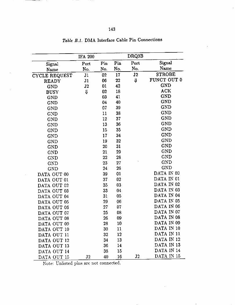
143
Table B.I. DMA Interface Cable Pin Connections
IFA 200 DRQ3B
Signal Port Pin Pin Port SignalName No. No. No. No. Name
CYCLE REQUEST J1 02 17 J2 STROBE
READY J1 06 22 _ FUNCT OUT 0
GND J2 01 42 GND
BUSY _ 02 18 ACK
GND 03 41 GND
GND 04 40 GND
GND 07 39 GND
GND 11 38 GND
GND 12 37 GND
GND 13 36 GND
GND 15 35 GND
GND 17 34 GND
GND 19 32 GND
GND 2O 31 GND
GND 21 29 GND
GND 22 28 GND
GND 23 27 GND
GND 24 26 GND
DATA OUT 00 39 01 DATA IN 00
DATA OUT 01 37 02 DATA IN 01
DATA OUT 02 35 03 DATA IN 02
DATA OUT 03 33 04 DATA IN 03
DATA OUT 04 31 05 DATA IN 04
DATA OUT 05 29 06 DATA IN 05
DATA OUT 06 27 07 DATA IN 06
DATA OUT 07 25 08 DATA IN 07
DATA OUT 08 26 09 DATA IN 08
DATA OUT 09 28 10 DATA IN 09
DATA OUT 10 30 11 DATA IN 10
DATA OUT 11 32 12 DATA IN 11
DATA OUT 12 34 13 DATA IN 12
DATA OUT 13 36 14 DATA IN 13
DATA OUT 14 38 15 DATA IN 14
DATA OUT 15 32 40 16 32 DATA IN 15
Note: Unlisted pins are not connected.
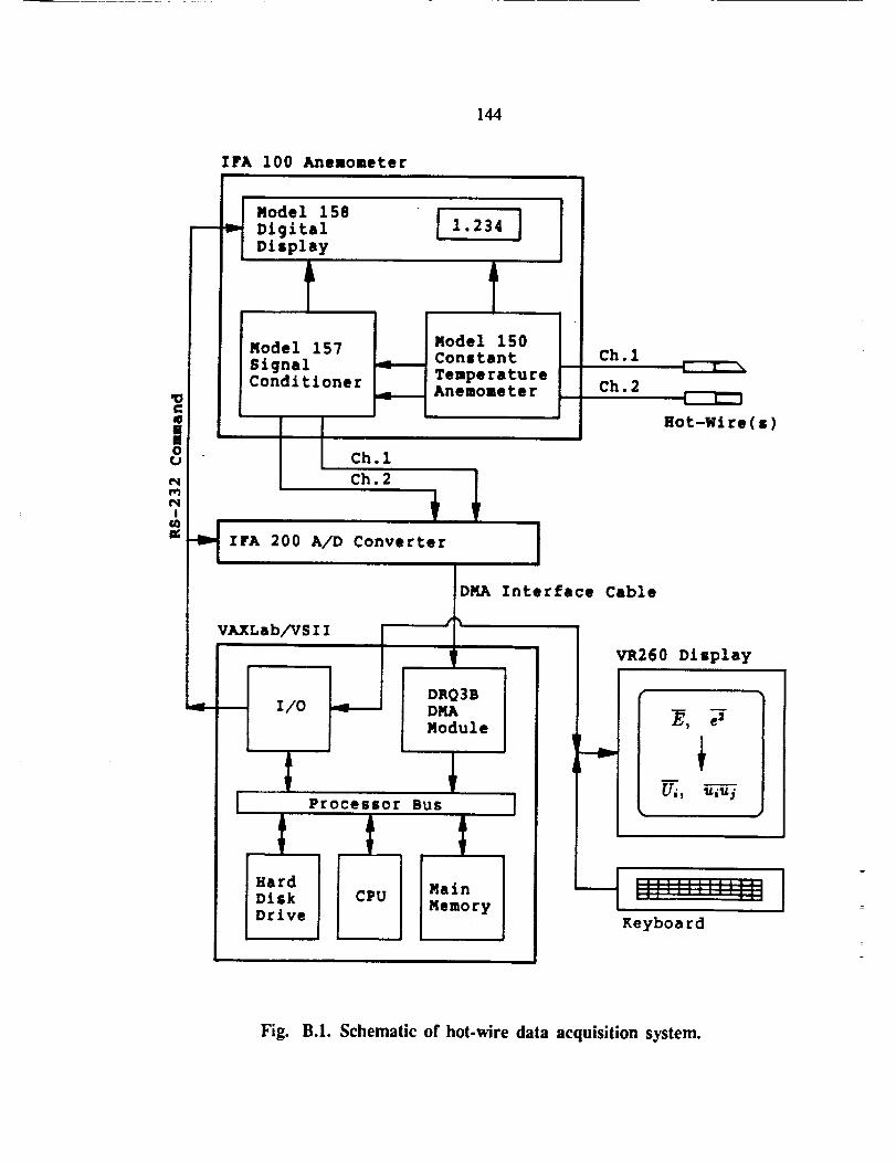
144
JOU
e4
N!
%PA 100 Anemometer
Model 158
DigitalDisplay
AL
Model 157
SignalConditioner
Model 150Constant
TemperatureAnemometer
Ch.l
Ch.2
Hot-Wlre(a)
Oh. i
Ch. 2
+_ IFA 200 A/D Converter
Ip-
VAXLab/VSII
-- I/0
Hard
DiskDrive
DMA Interfa¢
Processor BUS
DRQ3BDMAModule
CPU MainMemory
r
Cable
VR260 Display
w
m_ e2
+
i_.._ iii+_;+i.;+iiiiKeyboard
Fig. B.I. Schematic of hot-wire data acquisition system.
APPENDIX C
HOT-WIRE TECHNIQUES
C.1 Introduction
The derivation of the mean and turbulence hot-wire response equations for
the Method A technique are presented in this appendix. The working form of the
mean and turbulence response equations developed by A1-Beirutty (Method B)
are presented in this chapter without derivation. For details of the development
of these equations, the reader is referred to references [45] and [46].
The Method A single rotatable hot-wire technique which is proposed here
is applicable for the measurement of the mean flow and Reynolds stress field
in situations when the primary flow is nominally normal to the probe axis of
rotation. This, in itself, is not unique. De Grande and Kool [61] proposed a hot-
wire technique in which a single rotatable slant-wire is used to deduce the mean
flow and turbulence field under similar conditions. Their technique is not based
on an empirical cooling law relation, but rather relies on extensive pitch and yaw
calibration. The time required for calibration becomes prohibitive when large
amounts of data are being accumulated and frequent recalibration is necessary.
Their technique has the advantage that commercially available probes can be
used. The use a single slant-wire probe limits the range of sensitivity to the
individual mean velocity and stress components. This is usually compensated
for by obtaining data at a large number of rotational positions and using least-
squares error minimization criteria to solve for the flow variables. The hot-wire
technique proposed here relies on the sequential use of custom-made normal and
slant-wire probes in order to maximize sensitivity to the flow variables. The
response of the hot-wires to pitch and yaw flow angles is governed by an effective
cooling velocity relation so that only a simple calibration procedure is required.
Before continuing, it is important to note a restriction associated with
Method A that is not present with Method B. Whereas with Method B, for zero-
to-moderate skew angles, the probe body can be rotated 360 ° with little or no
interference effects from the probe supports, there is a significant region of rota-
tion associated with Method ,4 where interference effects from the probe supports
cannot be neglected. Within this region, no valid data can be expected; how-
ever, the angular sweep of this region can be minimized and the angular position
shifted by suitable design of the hot-wire probe itself. Two possible slant-wire
probe configurations, along with an estimate of their regions of interference for
use with Method A are illustrated in Fig. C.1. The impact of this restriction on
Me_hod A will be discussed as the response equations are developed.
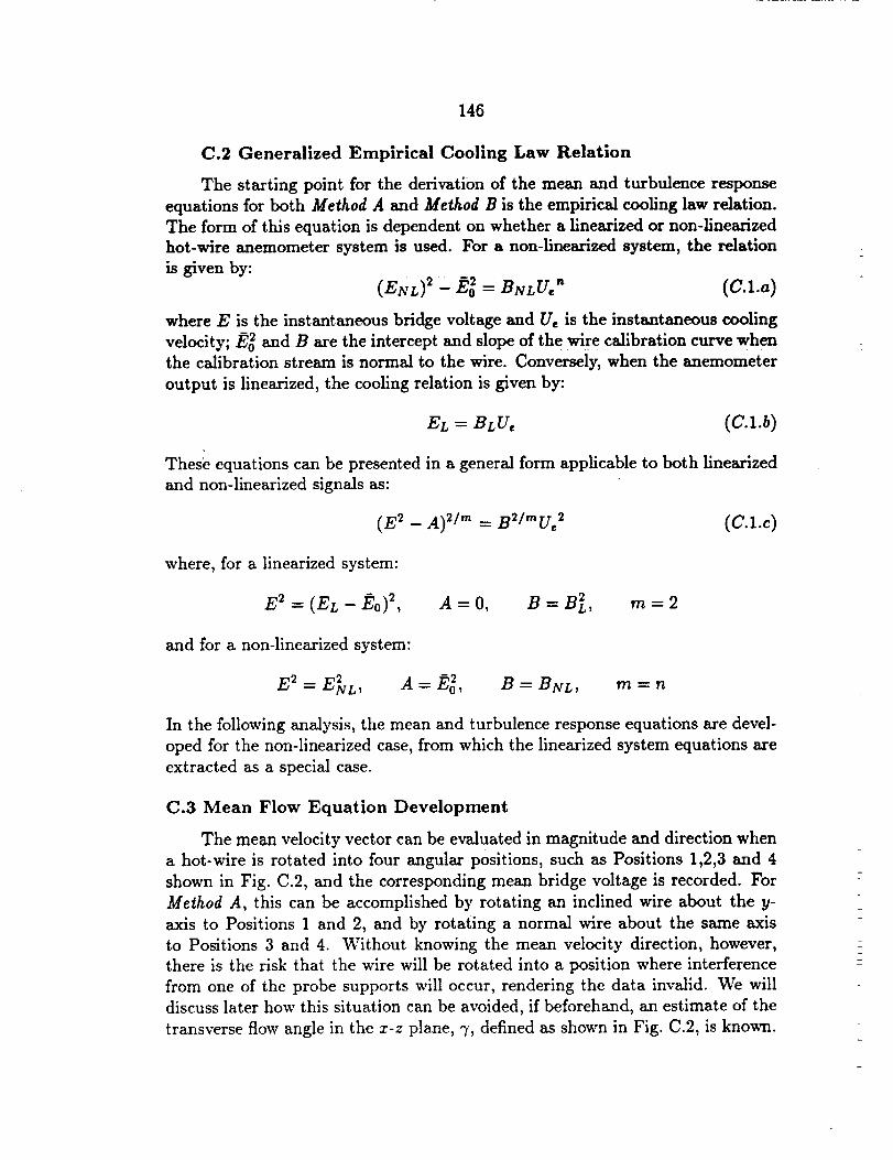
146
C.2 Generalized Empirical Cooling Law Relation
The starting point for the derivation of the mean and turbulence response
equations for both Method A and Method B is the empirical cooling law relation.
The form of this equation is dependent on whether a linearized or non-linearized
hot-wire anemometer system is used. For a non-linearized system, the relation
is given by:
(ENL) 2 E20 -- BNLUe n (C.l.a)
where E is the instantaneous bridge voltage and [7, is the instantaneous cooling
velocity; E0_ and B are the intercept and slope of the wire calibration curve when
the calibration stream is normal to the wire. Conversely, when the anemometer
output is linearized, the cooling relation is given by:
EL = BLUe (C.l.b)
These equations can be presented in a general form applicableto both linear]zed
and non-linearized signals as:
(E 2 - A) 2/'' = B21mUe2 (C.l.c)
where, for a linearized system:
E 2 = (EL - Eo) 2, A = O, B = B2L, m = 2
and for a non-linearized system:
E 2 = E2NL, A = E_, B - BNL, rn -- n
In the following analysis, the mean and turbulence response equations are devel-
oped for the non-linearized case, from which the linearized system equations are
extracted as a special case.
C.3 Mean Flow Equation Development
The mean velocity vector can be evaluated in magnitude and direction when
a hot-wire is rotated into four angular positions, such as Positions 1,2,3 and 4
shown in Fig. C.2, and the corresponding mean bridge voltage is recorded. For
Method A, this can be accomplished by rotating an inclined wire about the y-
axis to Positions 1 and 2, and by rotating a normal wire about the same axis
to Positions 3 and 4. Without knowing the mean velocity direction, however,
there is the risk that the wire will be rotated into a position where interference
from one of the probe supports will occur, rendering the data invalid. We will
discuss later how this situation can be avoided, if beforehand, an estimate of the
transverse flow angle in the x-z plane, 7, defined as shown in Fig. C.2, is known.
147
The reader should keep in mind that this is strictly a physical limitation and not
a restriction inherent in the response equations themselves.
For Method B, the four wire positions shown in Fig. C.2 can be achieved
by rotating a single inclined wire about the x-axis. Unlike Method A, for zero-
to-moderate skewness levels, the problem of probe support interference does not
present itself with Method B, and, therefore, no knowledge of the mean flow
direction is required apriori, other than that the flow is nominally in the x-
direction and that V and W are less than U.
The primary difference between Method A and Method B is in the expressions
for the effective cooling velocity term in equation (C.l.a). In the remainder of
this section, the mean flow response equations for both Method A and Method B
will be presented. Except where noted, the following discussion is applicable toboth of these methods.
When the time-averaged form of equation (C.l.a) is applied at each wire
position shown in Fig. C.2, the following four response equations result:
(.E,_- ._)_/,,, = BW"(U2),
(E_2_ ._)2/,,, = B_/,,,(U2)_
(E_ _ ._)2/,,,= B2/,,,(U_)_(E, 2_ _02)2/m= B2/",(U.2),
(C.2.a)
(C.2.b)
(c.2.c)
(C.2.d)
Combining equations (C.2.a) &: (C.2.b) and equations (C.2.c) & (C.2.d)
(,_12 -- F__2o)2/m/(E22 -- Eo2)2/m = -(Ue2)l/(Ue2)2
yields:
(C.3.a)
(z__- _,_,)_/" /(E,_- ._)_/" = (uJ)_/(uJ),,
Rearranging equations (C.3.a) and (C.3.b) gives:
(uJ)_-s,_(u,2)2= 0 (C.4.a)
(U._)3- _s4(U,2)4 = 0
where, for convenience, the following definitions are employed:
(C.4.b)
s,2 = (E,2- _0_)_/m/(E2_- _o_)_/_ (C.5.a)
_34= (E3_ - _,_,)_/"/(E,2- _,)_/"_ (c.s.b)
By eliminating the dependence on the wire calibration slope (B) in equations
(C.4.a) and (C.4.b), we have placed the restriction that the same hot-wire must
148
be used in Positions 1 and 2, and, likewise, in Positions 3 and 4. We do not
require, however, that the hot-wire that is used in Positions 1 and 2 be the
same as the one used in Positions 3 and 4, so long as the appropriate calibration
intercept values are used in equations (C.5.a) and (C.5.b):
In order to solve equations (C.4.a) and (C.4.b) for the mean velocity com-
ponents, the effective cooling velocity (U,) must be expressed in terms of the
mean velocity components (U, V, W), and the voltage terms (Ei_2, Es4) must be
expressed in terms of measurable mean (E) and mean-square (e 2) voltages.
•The voltage terms, E12 and E34, in equations (C.4.a) and (C.4.b) can be
expressed in terms of measurable voltages by substituting E = E + e into (E 2 -
E02)2/', expanding the resulting expression in a binomial series, and truncating
at second order:
e/_ Ce2(E'-F_,g)2/'=(.E2-F_,g)2/'[l+(41m)__,2__g + _2__o2 ] (C.6.a)
where:
E_C=2/m+(4/m)( - 1)(_2 _ _02 )
Time-averaging this expression yields:
(E=- gg)_/-_= ($_ - &_)_/=[1+
(C.6.b)
Ce 2
_ _ Eo_] (C.6.c)
Substituting equation (C.6.c) into equations (C.5.a) and (C.5.b) gives:
r_12= r_i/_2 (C.7.a)
where:
el el 2
:_,= (&__ &_)_/,-[_+ _ - _1
C2 c2 2
:_ = (_ - ,&_)_/,-[_+ E_- _1v
I
03e32
_:_= (_ - &_)_/,,,[_+ ._ - E_]04e42
S4 = ('E'_ - -Eo2)2/"[ 1+ _42 _ _021
(c.7.b)
(C.7.c)
The exact expression for the effective cooling velocity term, Ue 2, in equations
(C.4.a) and (C.4.b) can be expressed in terms of the mean velocity components
149
(U, V, W) and the Reynolds stresses (u-7_, i,j = 1,2,3) at the four wire positions
shown in Fig. C.2. as follows (recalling that different expressions are required for
Method A and Method B):
[Method A I (see Appendix D for derivation)
w
__ V 2
_= [(v)'+(U,2), =Ko,iU2{K,,,[I + _-{]+ -O-g]
+ K_,,sN[(-ff) + _1 +
(C.8.a)
v2(-U-j2)2=KoaU2{KI,2[1 + _-g]+ [(_) + _--_]
+ gzah_g[(W) 2 + U 2 U)+ _-_1}
. 21 _-_('Ue2)3 =Ko,sU {_(KI,a + h2ngKs,s)[1 + -_1
V _ 1 W)2 w2+ [( )2 + _-'_l + _(K,,a + h2BNKa,a)[("_ + -U-'_]
2 W- (K,,3 - hBNK3,z)[("-_-) + _-'_1}
(C.S.c)
m
1/2
(U¢_), =Ko,4U2{_(K1,4 + h2BNK3,4)[1 + -_]
"_ 1 K h2BNKa,4)t(W) 2 + w2+ [(v)= + _1 + _( .,, + _1
" -- hBNI{.3,I)[(-'O- ) Jr _---_']}+ (K,,4 = . W _-_
(C.S.d)
]Method B[ (see Appendix A, reference [47] for derivation)
_ U)2 v_(Ue2)I =I'(o,IU2{[1 _- _--_]-_ KI,I[( + _-_]
IV)2 w2 V _'_+K3,,h2BN[(--_ +_--_1+2K2,,[( )+_-_]}
(C.9.a)
150
132
t,2 K1,2[(V)2+(U+2)2=go,2U2{[1+ -_1 + -U-_]
2 w 2 _ [(u) + _]}+ K3,2hBN[(_-) + _-_]- 2K2,2 v2
(c.9.b)
m m
u2 V 2 132](U,2)3 =g0,3U 2{[1+ _-_] + K3,3h_N[(-_) + _._
,1,2]+K1,_[(w)2+ u2 + 2K2,3[(W) + _-_] }
(C.9.c)
u2 re" h 2 r,'V32 v2(U,2)4 =Ko,,tU 2 {[1 + _-'_] + ,,3,4 BNtt _': + _"_]
W)2 _ 2K2,,[(W+ K1,4[(-_- + _--_]- _-) + _']}
(C.9.d)
where K0, K1, K2 and//'3 (the second subscript denotes wire position) are func-
tions of the wire inclination angle (a), the normal cooling coefficient (h_¢) and
the tangential cooling coefficient (k); and hnN is the binormal cooling coeffi-
cient. The functional forms for these variables are given in Appendix D. When
equations (C.8.a) through (C.8.d) or equations (C.9.a) through (C.9.d) are sub-
stituted into equations (C.4.a) and (C.4.b), the following non-linear algebraic
equations, applicable to both Method A and Method B, result:
I(ov + Klv(V/U) + K2v(V/U) 2 + K3,,(W/U) 2 + Cv = o (C.10.a)
Ko_ + K,_(W/U) + K_(W/U) 2+ K_(V/U) _+ C_ = 0 (C.10.b)
whereu 2 _ v 2 w 2
c_ = Ko_(_--_) + g,,,(_-_) + K2,,(_-_) + K3,,(_--_) (C.11.a)
m m w
. U 2 . . U_ W 2 l) 2
c= = I;0w(_--_) + x;,=(_-_) + g2=(_-_) + g3w(_-_) (C.ll.b)
and where, for convenience, the following definitions have been employed:
_ethod AJKot, = Ko,l Kl,1 - Ko,2 K1,2 E12
Klo =2K0,1K2,1 + 2K0,2K2,2E12
h'2v =K0,_ - K0,2E12
K3_ =hBN(Iio,lI;3,1 -- Ko,2K3,2E12)
(C.12.a)
151
and,I r p" 2
Kow=(_)[Ko,3(_,_ + hBNN3,3)2
- Ko,_(KI,, + hBNK3,41:34]
+ Ko,4(K1,4 2-- hBNK3,4_34 ]
K_w =Ko,,,
I':3,,,=Koa - Ko,, _.34
(C.12.b)
and,
[Method B]
KOt)
Klv
K2.
K3,,
=Ko,a - Ko,2_12
=2Ko,1K_,l + 2KoaK2,2E]2
= Ko,1KI,a - Ko,_K1,2E]22 ,"
=hBN(I_o,IK3,1 -- Ko,2K3,2Ea2)
(C.13.a)
_w
_w
_w
--/(0,3 -- Ko,4 Y]34
--21(0,3I(2,3 q- 2Ko,4K2,4_34
= Ko,3 K1,3 -/(0,4K1,4_34
-- h 2BN( Ko,3 K3,3 - ]x_0,4K3,4 _34)
(C.13.a)
The terms Cv and Cw in equations (C.10.a) and (C.10.b) account for the errors
which would result from neglecting the fluctuating velocity components relative
to mean components in the expression for the effective cooling velocity.
In a low turbulence intensity field (< 10%), the correction terms Cv and Cw
in equations (C.10.a) and (C.10.b) can be neglected without introducing serious
errors in the computed mean velocity ratios (V/U) and (W/U). Under these
conditions, the mean response equations reduce to:
Ko,, + K1,,(V/U) + K_,,(V/U) 2 + K3,,(W/U) 2 = 0 (C.14.a)
Ko,, + KI,,,(W/U) + K2w(W/U) 2 + K3w(V/U) 2 = 0 (C.14.b)
Equations (C. 14.a) and (C.14.b) represent two coupled non-linear algebraic equa-
tions which can be solved simultaneously for the relative mean velocity compo-
nents (V/U) and (W/U). When second-order mean velocity terms in equations
(C.14.a) and (C.14.b) are neglected, solutions for (V/U) and (I¥/U) which are
first-order accurate may be obtained directly as:
(v/U)o = -KodK_.(tWU)0= -X;ow/K_.,
152
which are appropriate for evaluating (V/U) and (W/U) in slightly skewed flows.
For the more general case, however, equations (C.10.a) and (C.10.b) represent two
non-linear algebraic equations in seven unknowns (V/U, W/U, ui/U 2, v2/V _,
"_-i/U2, _-6/U 2, _'C/U2). Therefore, five more independent equations are required
for closure, which, in turn, requires rotation of the slant and/or normal-wire to
at least five different positions. If this is done arbitrarily, then the coefficient ma-
trix may become ill-conditioned. In order to overcome this difficulty, equations
(C.14.a) and (C.14.b) are first solved for the mean component ratios (V/U) and
(W/U) after initial estimates are made using equations (C.15.a) and (C.15.b).
The calculated results are then used to solve the turbulence response equations
(to be developed shortly) for the complete Reynolds stress tensor. The calculated
stresses can then be used to correct the mean velocity components by simulta-
neously solving equations (C.10.a) and (C.10.b). The improved mean velocity
values are subsequently used to update the Reynolds stress tensor. This iteration
proce.dure is repeated until convergence is achieved.
Once the mean velocity ratios (V/U) and (W/U) are known, the axial mean
velocity (U) can be determined by averaging its calculated value with the wire
at each of the four positions shown in Fig. C.2. When the expression for the
effective cooling velocity at Position 1 (equation (C.8.a) or (C.9.a)) is substituted
into equation (C.2.a), the following equation for the axial velocity with the wire
at Position 1 is obtained, after some rearrangement:
[- t odAI
u, ={(g2 _ _,o_)2/m[1+ C,F,_I(_,[- g2,)]I(Bo)_/'}'/_
v_.__ ] h _ [(-_--)_ + w'_{K,,,B + _] + + g_,, _NV _"-_11_1/2
+ 2,r_., 1 [(_.) + _.,
(c.16)
[Method B 1
u, ={(&_ - _7)_/-'[a+ c,7,_/(_,_,- t,2,)]/(B<)'/m}'/_
u''_ V 2 v"2 U w-"_{[1 + _-_] + .KI,,[(_-) + _--_] + K3,ih_N[( )2 + -_-7]
I/" u"'_1l-1/2+ 2s,_,,[(_) + _,,
where Be, the slope of the calibration curve, is either:
(C.17)
Bc = B (C.18.a)
153
when the calibration stream is normal to the wire, or:
Bc = B(K0) =/2 (C.18.b)
when the calibration stream is aligned with the probe body (as in Method B), or:
Bo = B(KoK, )"/_ (C.18.c)
when the calibration stream is aligned normal to the probe body (as in Method A).
Similar expressions for .the axial mean velocity can be derived for wire Positions
2, 3 and 4.
The total mean velocity (U0) is related to the axial mean velocity (U) by:
Uo = U� cos ¢ (C.19.a)
where,
¢= tan-l(vr/v)
vr/v = [(v/v) _+ (w/v)_] _/_
This section will be concluded with an explanation of how the possible probe
support interference associated with Method A can be avoided if data are taken
by means of probe rotation about the y-axis and an estimate of the transverse
flow angle 7 in the z-z plane is known.
Interference can be avoided if, rather than recording data relative to the
primary coordinate system, data are collected relative to a another coordinate
system which is rotated about the y-axis through an estimated yaw flow angle
70, which is close to the actual flow angle 7, such that the transverse velocity
component in the x-z plane is small. This allows the use of a hot-wire probe
body designed to tolerate small amounts of unknown yaw skewness. The mean
velocity components are computed by the method described above, relative to
the secondary coordinate system, and then they are transformed to the primary
coordinate system. Estimates of 70 can be established, at least to first-order
accuracy, by pressure nulling of a two-tube Conrad probe, or by means of the
hot-wire nulling technique described by Page [62].
C.4 Turbulence Equation Development
As was the case for the development of the mean response equations, the
starting point for the turbulence response equations is the instantaneous empir-
ical cooling relation:
(E 2 - t_o)_/"_= B2/mV, 2 (C.l.c)
154
Also, as before, the left-hand side is expanded by means of the binomial theorem
and truncated at second-order:
e_
(E2- _0_)2/m= (_ - _0_)_/m[x+ (4/m) _ _ E0_Ce 2 .
+ (C.6.a)
where,
C = 2/m + (4/,,',)( 2 _ 1)(£_ _ ) (C.6.b),,, _,o_In Contrast to the mean velocity development, the effective cooling velocity term
in equation (C.l.c), is derived relative to another orthogonal coordinate system.
For Method A, this coordinate system, x_,y,z _, is generated by a rotation about
the y-axis such that the x'-axis coincides with the resultant mean yaw velocity
vector, Ur (refer to Fig. C.3.a). For Method B, a coordinate system, x,y_,z ', is
generated by a rotation about the x-axis such that the z' = 0 plane coincides with
the resultant mean transverse velocity vector, Vr (refer to Fig. C.3.b). These new
coordinates are employed here because the Reynolds stress components, when
calculated relative to these new coordinates, do not involve the solution of a
full 6 × 6 system of equations under certain conditions. The exact forms of the
instantaneous effective cooling velocity relative to these new coordinates are:
[Method A] (see Appendix E)
u,== KoV,.={f,.+ f,,(,,'/V,.)+ f,,(vlV,.)- f.(w'/V,.)
+ K,_(,.,'=IV.2)+ (v=/V,.2)+ K, (w'=/V,.=)+ 2K,o(,;v/U2) - 2g,_(,,'w'/U,?)_ 2K,,(v_'/U,.=)}
(C.20)
where,
fm = Ka2 + 2Klo(V/U,.) + (V/U,.) 2
f. = 2K12 + 2Kao(V/Ur)
f_ = 2K10 + 2(V/Ur)
fw = 2K13 + 2Kll(V/U,-)
(C.21)
[Method B] (see Appendix B, reference [451)
Ue 2 = I;oU_{f,,,+/.(_,/u) +/,,(v'/u) + f_,(w'/U) + (,,2/u=)
+ I(12(v'2/U 2) + Z14(wt2/V 2) + 2Kao(Uv'/U 2)
+ 2K_a(uw'/V 2) + 2Kls(v'w'/U2)}
(C.22)
155
where,
f,, = 1 + 2Klo(V,./U) + K12(V,.]U) 2
f, = 2 + 2Klo(Vr/U) (C.23)f,, = 2Klo + 2IQ2(V,./U)
f,,, = 2KI_ + 2K_3(V,./U)
where K10, Kn, K12; K13, K14 are functions of the probe rotation angle, 0, and
of K1, K2 and K3, which, in turn, are functions of hN, k and a (refer to Appendix
D and E for explicit forms), and u _, v _ and w _ are velocity fluctuations along the
x', y' and w' axes, respectively, as shown in Figs. C.3.a and C.3.b. If equation
(C.6.a) and either equation (C.20) or (C.22) is substituted into equation (C.I.c)
and subsequently time-averaged, then the resulting expression would not take
into account first-order effects in the fluctuations and would, therefore, not be
appropriate for analyzing low intensity flowsl Also, the resulting set of equations
would form a 6 x 6 system of equations whose solution can lead to inaccuracies in
the calculated Reynolds stresses. In order to avoid these shortcomings, consider
equation (C.l.c) which is first time-averaged to yield:
( E 2- .E2o)2 /" = B21"_'ff'_, _ (C.24)
and then consider the difference between equations (C.l.c) and (C.24) in a nor-
malized form which eliminates the contribution of the slope factor, B 21", namely:
(E _ - E0_)_/m -(E2 - _0_)_/m U, _ _b--'_= -- (C.25)
On the basis of equations (C.6.a) and (C.20) or (C.22), the time-averaged terms
in equation (C.25) can be written as:
Ce2 1
and,
[Method A]
u, = 1;ouJ {f., + + +
+ 2IQo(-d_v /U,. 2) - 2Kl,(u-'i-Jw, lV,fl)
- 2KIl(-_'_w_/U,.2)}
(c.26)
(c.27)
Method B]
U_2 = I(oU_{f,,, + (-_/U _) + KI_(-I'Z/U _) + X,:_4('J/U _)
+ 2IQo(-_7;v' /V 2) + 2IQ_(uu,i /U 2 ) + 2K_3(v-_w' /U2) }(c.2s)
156
If the appropriate terms developed thus far are substituted into equation (C.25)
an expression which has the following functional form results:
f(e, e2,-_,ui, uiuj, u-"_)=O, i,j = 1,2,3 ((7.29)
since all mean flow field variables are known from the previous mean flow analysis.
Equation (C.29) implies that in order to retain first-order fluctuation effects,
equation (C.25) should be squared and time-avernged:
= -- (6'.30)[(E_- _0_)2/']_ [U,_]_
Now, if the appropriate terms are substituted into equation (C.30), and the
squaring and time-averaging performed, then, retaining only second-order terms,
the following generalized turbulence response equations result:
tMethoaA] (se_Appendix E)
F..(u,2/uJ)+ F_v(_/u,_)+ Fw_(w"/uJ)(c.31)
+ F_,,,(-jr;I U,.2)- F,_(_-r_'/U, _) - F_w(_'/U, _) = F=._where,
F,,,, =/2 _ 2f,,_IIK]2
F,.,_ = f,.2 - 2 f,,,IIK]4
F,,,, = 2(ft, fv - 2fmIIK_o) (C.32)
F,,w = 2(f,,fw - 2f,,,IIgls)
F,,_ = 2(Gfw - 2f,,,IIKll)
F,_ = fm2II
[Method B l (see Appendix ]3, reference [45])
F""(-_i/U2) + F""(°'2/U2) + Fw"(w'2/U2) (C.33)
+ F,,_(d-_/U2) + F,,,_(-_'/U 2)+ F,,,.(_-_'/U _) = F,,,,.,where,
F,,,, -- fu 2 - 2fmII
F_ = f2 _ 2franK12
F=,_ = f2 _ 2fmIIK14
Fur, = 2(fufv - 2f_iIKlo) (C.34)
F,,w = 2(f,,fw - 2f,.,IIK]])
F,),,, = 2(Gfw - 2fmIIK]s)
F.,_ = fm2rI
157
with (applicable to both Method A and Method B),
[_E_/('¢_ - _:°_)_l (C.35)n = 06/m _)[1+ 2Ce-_1(_2- E0_)_l
and frn,f,, fv and fw are defined by equations (C.21) or (C.23). The compo-
nent e"_"in the numerator of equation (C.3._5)is a consequence of the first-order
fluctuation(e) in equation (C.6.a),while e2 in the denominator isa consequence
of the second-order fluctuation(e2) in this equation.
C.4.1 Low Turbulence Intensity Flow
For flows of low turbulence intensity,the second-order terms in equations
(C.6.a) and (C.20) or (C.22) can be neglected in comparison to the first-orderterms. Substitution of the first- order forms of equations (C.6.a) and (C.20) or
(C.22) into equation (C.30) yields the following turbulence response equations
applicable to low intensity flows:
[Method A] (see Appendix E)
w
fJ(u'-_/ur2)+ fJ(-_/ur 2)+ fJ(w'2/uJ)
+ 2f, f,(-J-vv/U_ u) - 2fufw(u-T-WW/U_ u) - 2fJw(-v--_w,/Ur 2) = rf,, 2
(C.36)
[Method B I (see Appendix B, reference [45])
m m
fJ(-_/u _)+ fJ(v,_/u _-)+ fJ(w'_/u _)
+ 2f, f,('_-_v_lU 2) + 2f, fw(-_-wTwr/U_) + 2f_f_(v-'i_w_/U2) = _rfm u
(C.37)
with (applicable to both Method A and Method B),
7: = (16/m2)[_-]_2/(]_ 2 - ]_o2)2]
In principle,the six components of the Reynolds stresstensor relativeto the
x',y,zI coordinates shown in Fig. C.3.a or to the x,y',z'coordinates shown in
Fig. C.3.b could be determined by applying data taken at six fixed probe po-
sitionsto equation (C.36) or (C.37), respectively,for low intensityflows. This
is possible,since,in general, the wire will be sensitiveto all three fluctuating
velocity components at a given rotation angle. The resulting6 x 6 system of
equations may, however, become ill-conditionedifthese fixedprobe positionsare
specified in an arbitrary manner.
To increase the accuracy of his calculations, AI-Beirutty employed a sensi-
tivity minimization criteria to Method B which significantly improves the condi-
tion number of the coefficient matrix. He accomplished this by observing that
158
at certain rotation angles ("optimum planes"), the wire is either insensitive to
a particular transverse velocity fluctuation, C or w _, or is equally sensitive to
both. As will be shown shortly, when data are taken at these optimum planes,
the resulting 6 × 6 system of equations becomes partially decoupled, and, as a
result, the problem is reduced to the solution of several lower-order systems of
equations. The behavior of the sensitivity coefficients in equation (C.30) will be
examined to determine if similar criteria can be applied to Method A as well.
The sensitivity coefficients f,, f_ and fw appearing in equations (C.36)
and (C.37) can be written in terms of the probe rotation angle 0 when the
appropriate expressions for the K10 through K14 coefficients (given by equation
(E.7) in Appendix E) are substituted into equations (C.21) and (C.23):
[Method A [
f, = 2(K1 cos 2 O + h_NKssin 2 O) + 2K2cosO(V/U,.)
fv = 2K2 cosO+ 2(V/U,.)
fw = 2(K1- hBNKs)2" sm" 6 cos 6 + 2K2 sin O(V/Ur)
(C.39.a)
(C.39.b)
(C.39.c)
lMethod BJ
f. = 2 + 2K2cosO(Yr/U)fv -- 2K2 cos 0 + 2(K1 cos 2 6 + h_NK3sin 2 O)(V,./U)
fw = 2K2 sin0 + 2(K1 - h_Ng3)sinOcosO(V,-/U)
(C.40.a)
(C.40.b)
(C.40.c)
In order to examine the wire's sensitivity to the fluctuating velocity components,
it is expedient to plot the Reynolds stress coefficients appearing in equations
(C.36) and (C.37) as a function of probe rotation angle (0) for various levels
of skewness. The normal and slant-wire cases for Method A are shown in Figs.
C.4 and C.5, respectively, and for Method B in Figs. C.6 and C.7, respectively,
utilizing typical values for the cooling coefficients: k = 0.15, hg = 1.0 and hBN
= 0.9. Note that for Method B, only positive skewness angles need be considered
since negative angles can be transformed to positive angles by a 180 ° rotation of
the probe.
[Method A J
In order for the hot-wire to be insensitive to the w' fluctuating velocity
component, the coefficient fw must be equal to zero. An examination of Fig. C.5
reveals that f_ is zero for a slant-wire at any skewness level when the wire is in
the 0 and 180 ° positions. These locations will be denoted as Positions A and B,
respectively. The offset prong slant-wire configuration (refer to Fig. C.l.b) was
designed to operate in these positions with minimal probe support interference.

159
For a normal-wire (see Fig. C.4), fw is zero at 8 = 0 ° and 270 °, although the
former position is not admissible due to interference effects. The latter position
is designated as position NA. The above conditions allow three of the..__Yn01ds
stresses to be calculated independent of the remaining three. The u _2, v'_ and
u'v stress components can be obtained by applying normal-wire data at position
NA and slant-wire data at Positions A and B to equation (C.36) and solving the
resulting 3 x 3 system of equations.
With three stress components known, attention is turned to the condition
when the wire is insensitive to the v fluctuating component, which occurs when
f_ is zero. For Method A, this condition proves of little use, inasmuch as for the
limiting case when the skewness is zero, the slant-wire positions where f_ = 0
correspond to positions where fw = 0, namely; 8 = 90 and 270 °. Also, for
the normal-wire, in general, there is no location where f_ = 0. The condition
where the slant-wire is equally sensitive to both transverse fluctuating velocity
components is also of little use. The reason for this is because the angular
locations where these conditions occur do not always coincide with, or are even
near, the maximum sensitivities of the unknown stress components. Therefore,
for Method A, it appears that fixed probe positions are necessary.
With reference to Fig. C.5.b, there are four fixed positions, 6 -- 45,135,225
and 315 °, designated as Positions EA, FA, GA and HA, where the slant-wire is
always strongly sensitive to the vw _ stress component, at least over the skewness
range considered. The straight prong slant-wire configuration (refer to Fig. C. 1.c)
was designed to operate in each of these positions with minimal probe support
interference. Slant-wire data taken at these four positions can be used to evaluate
the vw _ stress component directly. An algebraic expression (derived in Appendix
E) for this component is given as:
vw-"7 _[(f.f_)v,_(_rE,_--_rHA)(f_2)EA --(f.fu:)EA(IrFA --_rGA)(f,n2)FA]
= (2f,,f,,,)r.,(2f,,f,,,)E..- (2f,,f,,,)E,,(C.41)
At this point, expressions for four of the six Reynolds stresses have been devel-
oped and there are no more wire positions available that will further decouple
the response equations. Therefore, in order to get the remaining two Reynolds
stresses (w '2 and u--V_w_),at least two additional probe positions are required, and,
ideally, these positions should be at rotation angles where the sensitivity to the
unknown stresses is at or near a maximum. With reference to Fig. C.4.b, for the
normal-wire, two fixed positions exist where the wire is nearly equally sensitive
to both u _ and w wfluctuations, namely; 0 = 225 and 315 °, which are denoted as
Positions CA and DA, respectively. When normal-wire data at Positions CA and
DA and the four known Reynolds stresses are applied to equation (C____.36), then
a 2 x 2 system of equations results, which, when solved, yields the w '2 and u_w''''_
Reynolds stresses.
160
Method B]
With reference
condition f,_ = 0 is
Positions A and B,
to Fig. C.7, two slant-wire probe positions result when the
applied to Method B: 0 = 0 and 180 °, which are denoted as
respectively. The normal-wire also has two positions where
f,_ = 0:0 = 0 and 90 ° (refer to Fig. C.5). For the normal-wire, 0 = 0 has the
additional benefit that fv = 0 as well. This position is denoted as position NB.
When normal-wire data at position NB are applied to equatio..n.n (C.37) a single
algebraic equation for the u"T stress component results. The v '2 and uv"--7 stress
components can be obtained by applying slant-wire data at Positions A and B
to equation (C.37) and solving the resulting 2 x 2 matrix.
When the condition fv = 0 is applied to Method B, two discrete slant-
wire positions result, designated as CB and DB in Fig. C.7.a. At these positions,
which are not fixed, but rather vary with skewness level, the slant-wire is sensitive
only to u and w' fluctuations. If the u 2 stress component, which is known from
previous calculations, and slant-wire data at Positions Cs and DB are applied
to equation (C.37), then a 2 x 2 matrix results which may be solved for the w '2
and uw _ stress components. The remaining unknown stress component, v'w _, is
determined by solving an algebraic expression which utilizes slant-wire data at
Positions EB, FB, GB and HB shown in Fig. C.7.b. These four wire positions
correspond to locations where the wire is equally sensitive to both transverse
fluctuating velocity components, or, in other words, where fv 2 = fw 2. The
expression for v'w' (derived in Appendix C of reference [45]) is given as:
U 2 - (2f,,f,,)FB (2fvfw)EB -- (2.f,_f,,,)Et,(2f,,.fw)Fv
(C.42)
For all slant-wire measurements referred to Method B, the straight prong probe
configuration shown in Fig. C.l.c is adequate, since probe interference effects do
not occur with the wire in Positions A through NB, provided that the skewness
level does not exceed 30 ° in a low intensity flow and 20 ° in a moderate intensity
flow [45].
C.4.2 Moderate Turbulence Intensity Flow
The preceding analysis is applicable only to low turbulence intensity flows.
For the more general case, equation (C.31) or (C.32), as applicable, must be
solved. Second-order velocity fluctuations which appear in the expressions for
the effective cooling velocity (equation (C.20) or (C.21)) prevent the decoupling
of the stress components, so that a full 6 x 6 system of linear equations must be
solved.
161
[Method AJ
For Method A, slant-wire data at Positions A, B, CA and DA, in addition
to normal-wire data at position NA, result in a system of five coupled hnear
equations. The sixth equation is obtained by utilizing slant-wire data obtained
at Positions EA, FA, GA and HA. The generalized response equation (derived in
Appendix E) is given as:
(_ _,E., -- s_K_,F.,)(': /G,-_)+ (s_- _)(V/G,:)+
(slKa4,Ea - s2Ka4,fa)(w'2/U, .2) + 2(slK10,Ea - s_K,o,FA)('Q'_v/U,-_) -
( S,,,w - S2,,,,, )(-_w' /U,. 2) = --( sx f ,,,,Ea -- s2 f ,,,f a )/2
(c.33)where
s,= -S[(Lf,,,)F.,--(f.K,3)F.(nF_+ na.)l(nE_- nn.)(f.)E_s== -8[(L,/w)_- (I_K_3)E_(nE_+ nF_)](nv_--na_)(f.)F_
and,
s,_w= 16[(f,,.f,,,)r,,- K,_,F.(/.)F_(nF.+ na.,)]x
[(f,d,_)E,,- K,,,E_(.&)E.(rI_.+ n.,,)]
S2,,w = 16[(]_/w)Ea -- KlS,Ea(f,,)Ea(IIE., + IIHA)]X
[(f,,fw)Fa--A"I,,Fa (f,.)F., (YIF.4+ lrIGa)]
and where II is given by equation (C.35) and Klo through K14 are given by
equation (E.7).
[Method B[
For Method B, slant-wire data at Positions A, B, CB and DB, in addition
to normal-wire data at position NB, result in a system of five coupled linear
equations. The sixth equation is obtained by utilizing slant-wire data obtained
at Positions EB, FB, GB and Hs. The generalized response equation (derived in
Appendix C of reference [45]) is given as:
(s, - s_)(-J/u s) + (s, K_,_ - s_Ka2,F_)(v '2 �US)+
(s, Ka4,EB - s2.K,4,Fn )(w'2 /U 2) + 2(s,/Qo,EB - s2K, o,FB )('_-wi/U2)+
(S,,,_ - S2,,,.)(v--V_w'/U 2) = --(s, fm,E. -- s2fm,F. )/2
(C.44)
where
s, = --8[(f,f_,)FB -- K,,,FB(f,,)FB(II_'B + IIGs)](IIEn -- IIHn)(f,_)EB
s2 = --S[(Afw)Zs -- KII,Es(fm)EB(I'IEs + I'IH,)](I'IFB -- I-IGs)(fm)FB
162
and,sl w = 16[(f=fw)F.-- K ,,Fs(fm)F.(riF. + riGs)i×
[(fvfw)Es -- K13,Es(fm)Em(IIEa -[" IIH.)]
S2,w = 16[(fufw)Es - Kll,Ea(fm)Es(IIEs + I'IHa)]X
[(hfw)Fa -- gl3,Fs(fm)Fjs(IIFs Jr rigs)]
and where ri is given by equation (C.35) and /(10 through K14 are given by
equation (E.7).
C.5 Solution of Mean and Turbulence Equations
C.5.1 Low Turbulence Intensity Flow
For low intensity flows the velocity ratios V/U and W/U and, in turn, V/U,-
(Method A) or V,-/U (Method B), are found by applying the Newton-Raphson
procedure to the simultaneous equations (C.14.a) and (C.14.b). First-order ap-
proximations given by equations (C.15.a) and (C.15.b) are used as initial esti-
mates in the calculation procedure. Once V/U,. or V,-/U (as applicable) is known,
the optimum planes locations are determined from equations (C.39) or (C.40),
as applicable. Data can then be taken at these locations or interpolated to these
positions from data taken in fixed increments. These data are applied to equa-
tions (C.36) and (C.41), or (C.37) and (C.42) from which the Reynolds stress
components are computed relative to the secondary turbulence coordinate sys-
tem. The Reynolds stress tensor is then transformed to the primary coordinate
system.
C.5.2 Moderate Turbulence Intensity Flow
For moderate intensity flows, the velocity ratios V/U and W/U are com-
puted by simultaneously solving equations (C.10.a) and (C.10.b). These equa-
tions, however, require knowledge of the Reynolds stress components. To allevi-
ate this problem, V/U and W/U are first estimated by solving equations (C. 14.a)
and (C.14.b). From these results, optimum planes are established and Reynolds
stresses relative to the secondary coordinate system are computed using either
equations (C.31) and (C.43), or (C.33) and (C.44), as applicable. The stress
tensor is then transformed to the primary coordinates and substituted into equa-
tions (C.10.a) and (C.10.b) from which improved estimates of V/U and W/U are
calculated. These improved estimates are, in turn, used to update the Reynolds
stresses and so on until convergence is achieved.
A disad_-antage of the above procedure is that two slant-wire probe configu-
rations are required for Method A in order to obtain data at Positions A, B and
EA through HA. An alternative procedure would be to obtain slant-wire data at
three (or more) fixed positions; 0 = 45,225 and 315 °, all of which are attainable
with the offset prong slant-wire probe configuration shown in Fig. C.l.b. By
163
applying slant-wire data at these positions and normal-wire data at Positions
CA and DA to equation (C.36) the stress components, w '2, _ and vw' can be
solved so as to minimize the error (in a least-squares sense) associated with the
over-specified conditions. It should also be noted that in many practical flows,
the secondary shear stress v"-_ is at least an order of magnitude less than the
other stress components and can be neglected. Under these circumstances there
is no need for the straight prong slant-wire probe shown in Fig. C.l.c.
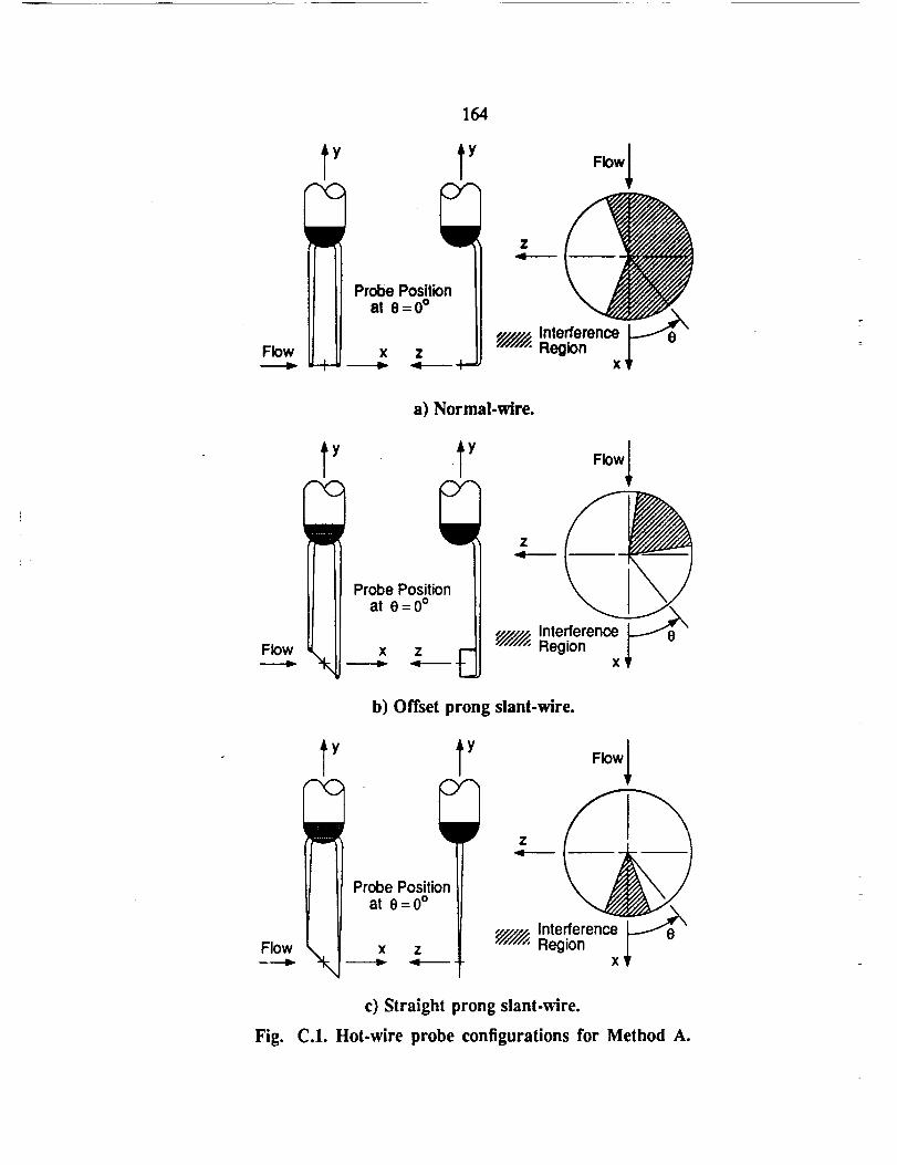
164
'Y t' ll Flow
a) Normal-wire.
I Y =l y Flow
II ,.__ ___
_ "/7///Z_"_te_?erenCex _\
b) Offset prong slant-wire.
c) Straight prong slant-wire.
Fig. C.1. Hot-wire probe configurations for Method A.
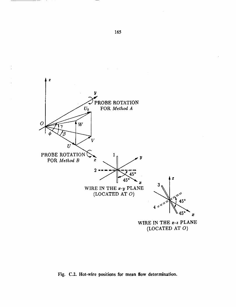
165
Z
Y
_'_ROBE ROTATION
_ FOR Method A
PROBE ROTATION t,,,"-,_FOR Method B x - "1]] jy
X
WIRE IN THE x-y PLANE
(LOCATED AT O)
Z
__ 45 °
Z
WIRE IN THE x-z PLANE
(LOCATED AT O)
Fig. C.2. Hot-wire positions for mean flow determination.
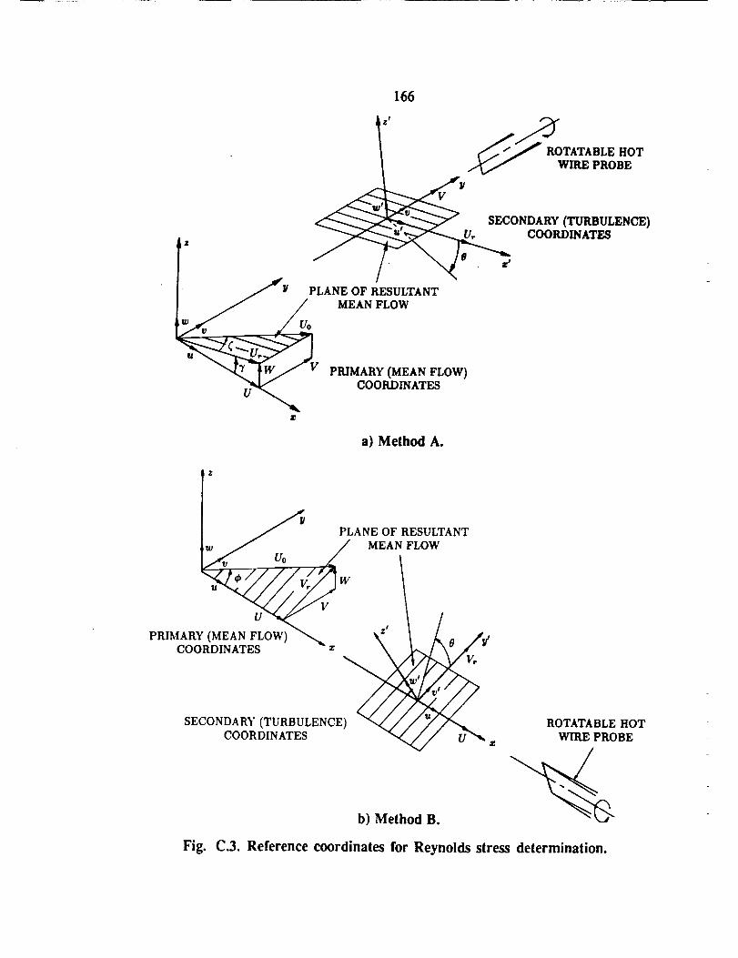
Z
166
ROTATABLE HOTWIRE PROBE
__U, SECONDARY (TURBULENCE)
COORDINATES
PLANE OF RESULTANT
MEAN FLOW
PRIMARY (MEAN FLOW)COORDINATES
a) Method A.
PLANE OF RESULTANT
__ / MEANFLOW
/__ /. _ ./z 1
PRIMARY (MEAN FLOW)_ _xz' 6' Jl/
COORDINATES - z . \ _V,"
SECONDARY (TURBULENCE)_
COORDINATES _ z
b) Method B.
ROTATABLE HOT
WIRE PROBE
Fig. C.3. Reference coordinates for Reynolds stress determination.
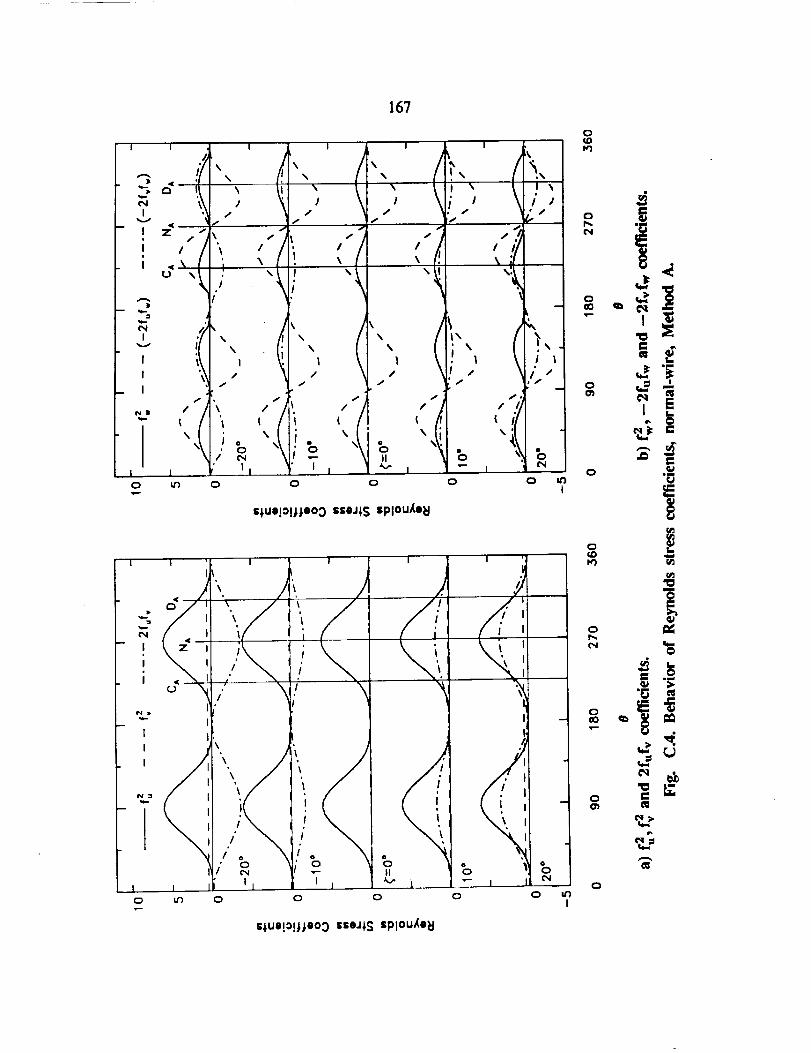
167
Iv
I
I
_ I
I _ I _ I I i I !
,, ,, ,, ..,!
I i / / , ,"ep i ,,e r_,,
:i:iiI Z //]\ _ /
I I/ I , I I
i ,
I
I,,111
I I
I I I , I/ / / I I
/ _ / : f
r i-
I I l "/I
\ i \
/. b "\ bI'M
' I I ' I
Q 0
I IM
\;,
i"z ==011 / _ "
o ,.,.,= --
II
1
o
t "(/ ""| / /'iI t
b b! I
o 0
=lue!ollleoo s;eJlS splouXell
I I ' I I I
", i )',.z ' '_
- !
, ! iii "d -_ ."': // __!" \
- I
I I'
I '\ l! _ [
I \ I' I'
I =
/ cM II
I 1 II I I '_" 1
o _ Q o o
I
/" I
i ii '
.L
! i! i
1 I ,t"q
0 0
° iI,DPc)
o Ig
c_
Q
I
;;ue!o!jleoo #seJlS #PlOUAe_l

168
1 I \!,,
"_ _. Jlx
_ /
-- I /J
I / !
I
_ I
J
0
\
//
/
\
i I• //
/
/
-'qO) .....
cN I _I
-// I
/
I
o o
,\/
I
//
I
I ; Io
\ /
.\/
//
/
,l ii
o
I
0 0 0
i/
/
/
i
\I
i \x
I/
/
//I,
1 "- !
o
s;uelol;;Oo 0 sseJJ,$ spl0u,_e_l
\
h
o o
s+ueloU_eo 0 sseJ;$ splou/,e_l
0
//
I/
/
/
'!," i" i
\
I
l/ --
0 0
I
\I
I
I
/ .
b
0 0
I
0_D
o.- I
or
° i_D
o 0
o
@
o
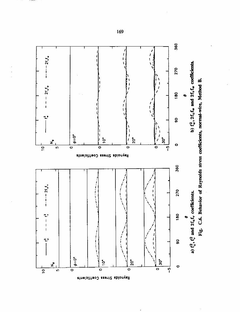
169
i I
ii
I
I
I
Nil
I I
I
I
i
I
I
I
bII
"0-
0
bII
-o-
0
I I I
/
I I
I I
b
o
I
i I
!i
/
/
I
I
I
Ibr e,4 !
0
s_uel01_;e0_)ssea_5 spl0uXeEI
I
J0°
II
II, ,
II
;qil• !
II
IZ
I
I
II,,
tl• !
II
11i I
! I
i
0
.I
01
! i! i
\
J
I
/
I
Ii
! ii ,
ooc,,,i
cD
m
i_ 1i -1
/ I
oo
I
o ._
!a
| I
/
/ I/ I
/' II
,
\, |\
\
.11/ l
/ II,/ I
i | -
\,I
bI I _
o u')I
0_De_
0
tE
m _T_
o
e_
o
s_uelall_eo:) ssea_$ splouXe_l
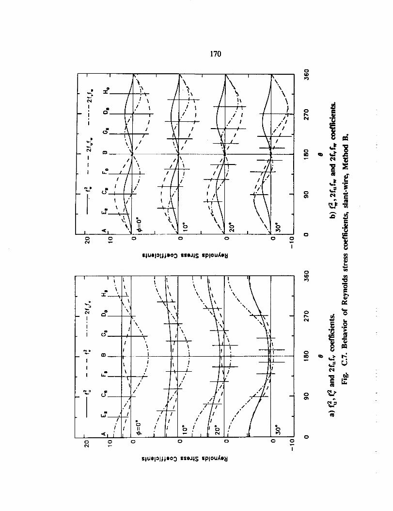
170
stuelOll;eo::) sseJ;S spIouAe_l
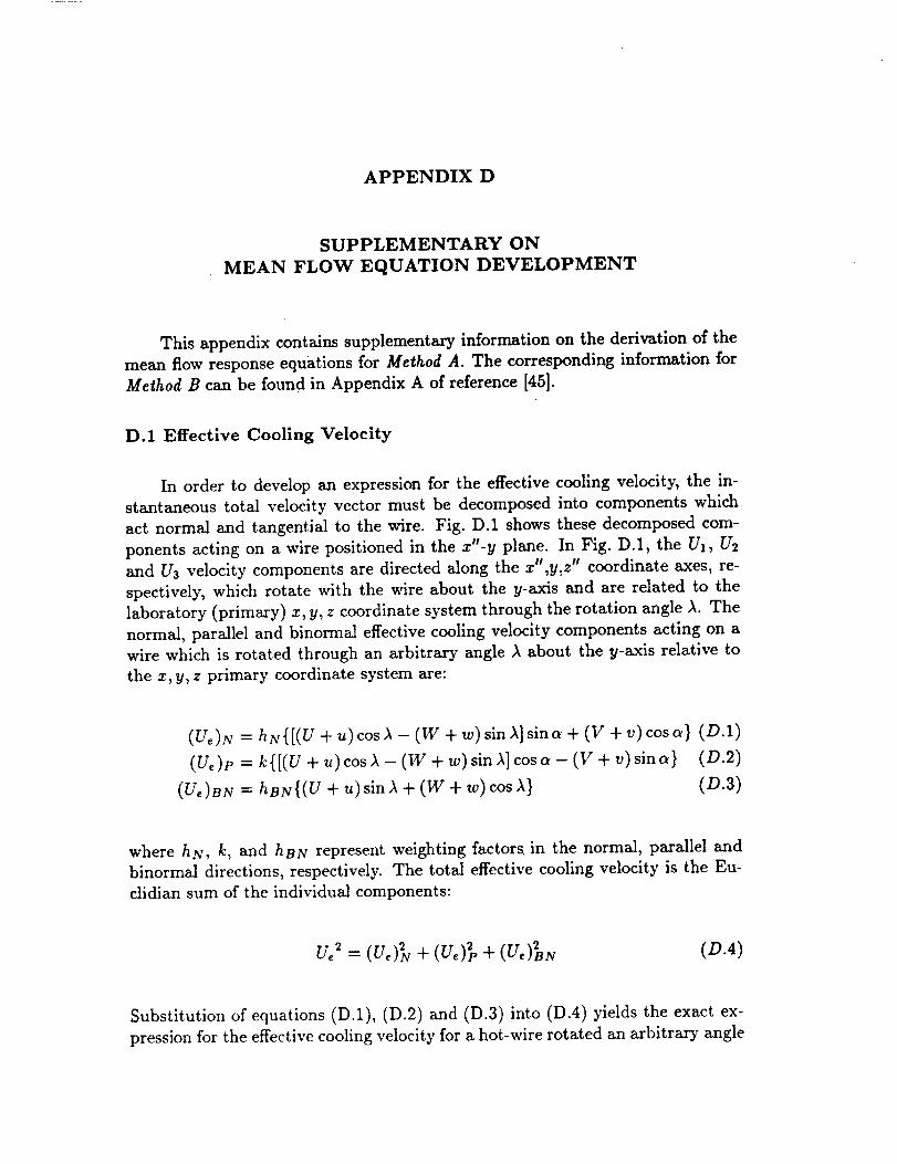
APPENDIX D
SUPPLEMENTARY ON
MEAN FLOW EQUATION DEVELOPMENT
This appendix contains supplementary information on the derivation of the
mean flow response equations for Mefhod A. The corresponding information for
Meihod B can be found in Appendix A of reference [45].
D.1 Effective Cooling Velocity
In order to develop an expression for the effective cooling velocity, the in-
stantaneous total velocity vector must be decomposed into components which
act normal and tangential to the wire. Fig. D.1 shows these decomposed com-
ponents acting on a wire positioned in the x"-y plane. In Fig. D.1, the U1, U2
and U3 velocity components are directed along the x",y,z" coordinate axes, re-
spectively, which rotate with the wire about the y-axis and are related to the
laboratory (primary) x, y, z coordinate system through the rotation angle A. The
normal, parallel and binormal effective cooling velocity components acting on a
wire which is rotated through an arbitrary angle A about the y-axis relative to
the x, y, z primary coordinate system are:
(U,)N = hN{[(U + u)cosA - (W + w) sinA]sina + (V + v) cosa} (D.1)
(U,)p = k{[(V + u)cosA-(W +w)sinA]cosa-(V + v)sina} (0.2)
(Ue)BN = hBN{(U + u)sin A + (W + w) cos A} (9.3)
where hN, k, and hBlv represent weighting factors in the normal, parallel and
binormal directions, respectively. The total effective cooling velocity is the Eu-
clidian sum of the individual components:
u,2= + + (D.4)
Substitution of equations (D.1), (D.2) and (D.3) into (D.4) yields the exact ex-
pression for the effective cooling velocity for a hot-wire rotated an arbitrary angle
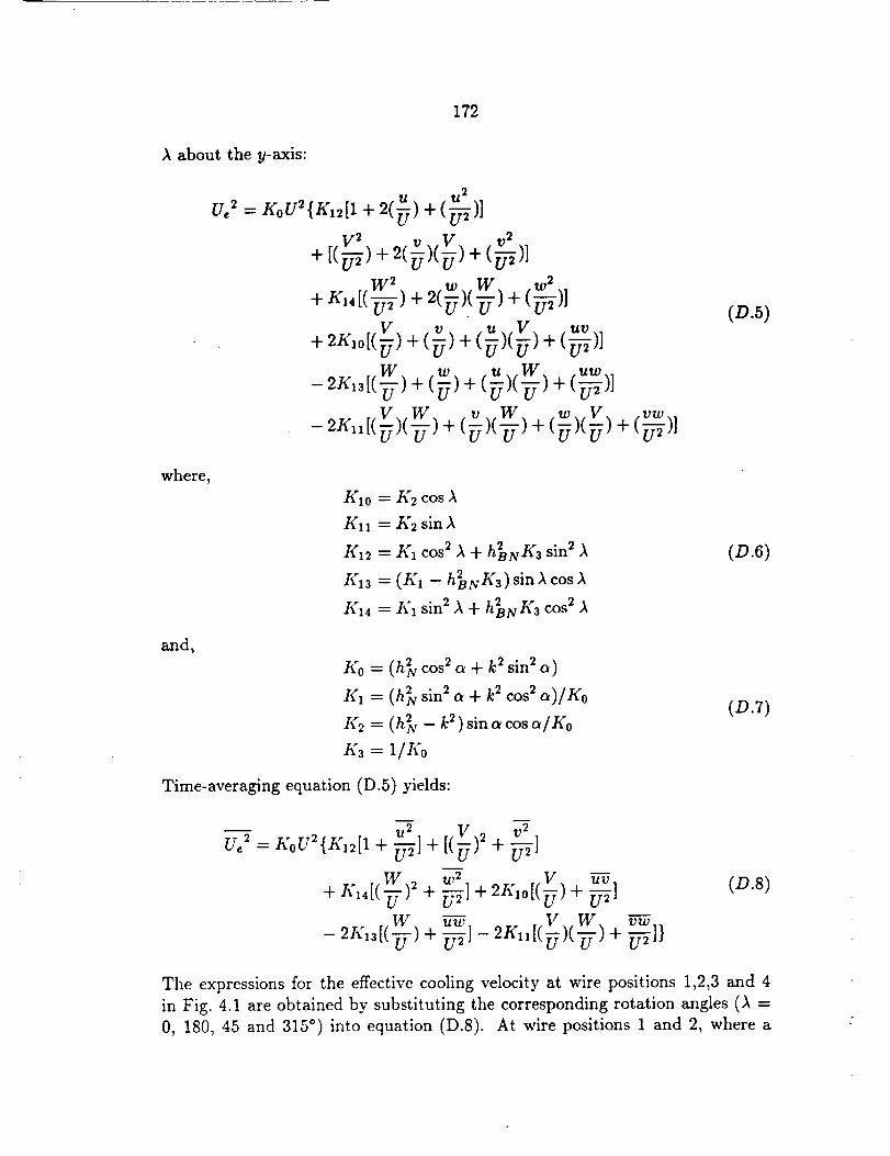
172
A about the y-axis:
U, 2
u 2
= KoU2{K12[1 + 2(U) + (_')]
v2 ]
W 2 w W -_2+ K,4 [('-U-T) + 2(_)(-_-) + ( )1
V v u V uv+ 2K10[() + (_) + (_)(_') + (_'_-)]
-2K_z[( ) + (_) + (_)(F) + ( )]
V W v W U vw- 2K11 [(_')(-_-) + (_)(--_-) + (U)() + (_-_-)]
(D.5)
where,
and_
K10 =/42 cos A
Ka 1 = K2 sin A
Ka2 = Ka cos 2 A + h_NKa sin 2
= hBN/{3) sin A cos AKI3 (KI- 2 -
K14 = IX'l sin 2 A + h2BNKa cos 2 A
K0 = (h_v cos 2 a + k 2 sin 2 a)
/(1 = (h_v sin 2 a + k 2 cos 2 oO/Ko
I,'_= (h_ - k_)sin,¢os,/A'0K3 = 1/Ko
Time-averaging equation (D.5) yields:
(D.6)
(D.7)
-- ,_] v _ v_U_2=KoU2{K,2[I+u 2 +[(_) +_-_1
w 2 . V
+ Kx4[(_--) 2 + _-_-] + 2K10[(_) + _-_]
W uw 2K11[(V)(W V-_- 2K,3[(_-) + b-_]- -K) + _]}
(D.S)
The expressions for the effective cooling velocity at wire positions 1,2,3 and 4
in Fig. 4.1 are obtained by substituting the corresponding rotation angles ()_ =
0, 180, 45 and 315 °) into equation (D.8). At wire positions 1 and 2, where a
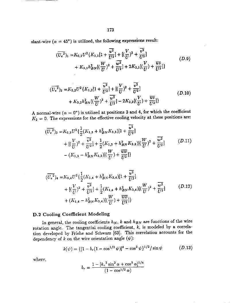
173
slant-wire (_ = 45 °) is utilized, the following expressions result:
!
[(y)_ _(Ue2)l =Ko,,U2{KI,I[ 1 + "_'-i] + + -U-'_]
r: h 2 [¢W_2 w2 2K2,1[(V)+ h--fi+ ,,_,,B_,_-ff,+ _1 + _1}
(D.9)
[(y)_ +(-g-:)2=Ko,,U2{KI,,p + _l + _l
h_ W _ _ [(Y) ++/Q,2 BN[('_-) + _-'_1- 2K_,2 _-_]}
A normal-wire (a = 0 °) is utilized at positions 3 and 4, for which the coefficient
Ks = 0. The expressions for the effective cooling velocity at these positions are:
1. K _-(U_2)3 =Ko,sU2{_( ,,s + h_BNgs,s)[ 1 + -_-il
-_] 1 2 K W2 w2+ [(v )_+ v_ + _(g,,3 + hBN 3,_)[(-ff) + _12 - W
- (I(1,a - hBNI(a,a)[(-ff) + _-_'1}
(D.11)
D
. 2 1 h2BNK3,4)[ 1+ u s(v_2), =I_0,,v (_(K_,, + _1
V)2 _ ½ W)2 w2+ [(U + U-"2]+ (K1,4 + h_NKS,4)[("ff + _--_1
W _'_+ (gl,, - hBNK_,,)[(-ff) + b-Z]}
D.2 Cooling Coefficient Modeling
In general, the cooling coefficients hN, k and hBN are functions of the wire
rotation angle. The tangential cooling coefficient, k, is modeled by a correla-
tion developed by Friehe and Schwarz [63]. This correlation accounts for the
dependency of k on the wire orientation angle (¢):
k(¢)= {[1-b_(1-cosl/2¢)]4-cos2¢}_/2/sin¢ (D.13)
where,1 - [k_ 2 sin 2 a + cos 2 a] 1/4
Dr
(1 - cosl/2 or)
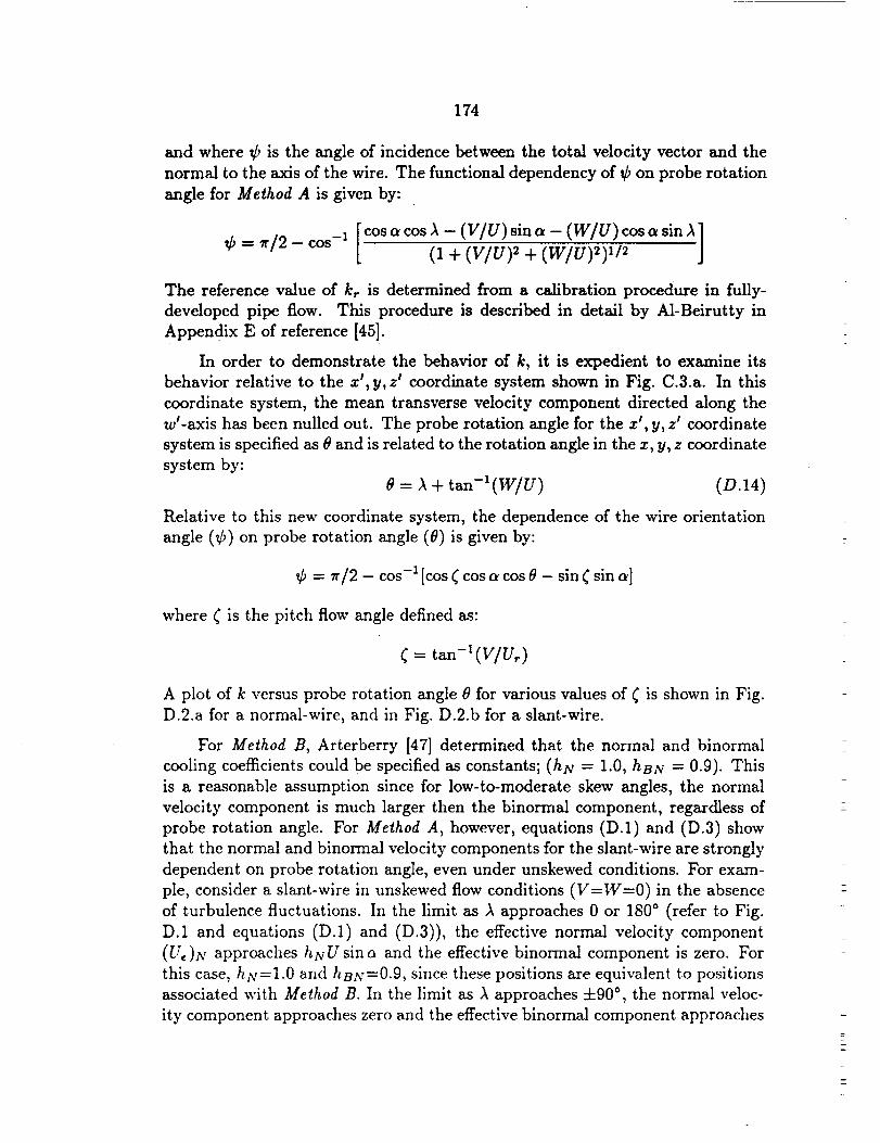
174
and where ¢ is the angle of incidence between the total velocity vector and the
normal to the axis of the wire. The functional dependency of ¢ on probe rotation
angle for Method A is given by:
[ cos a cos A - (V/U) sin a - (W/U) cos a sin A]¢ = , 12 - cos-' (1 + (VlU) +
The reference value of k r is determined from a calibration procedure in fully-
developed pipe flow. This procedure is described in detail by A1-Beirutty in
Appendix E of reference [45].
In order to demonstrate the behavior of k, it is expedient to examine its
behavior relative to the z', y, z' coordinate system shown in Fig. C.3.a. In this
coordinate system, the mean transverse velocity component directed along the
w'-axis has been nulled out. The probe rotation angle for the z', y, z' coordinate
system is specified as/_ and is related to the rotation angle in the x, y, z coordinate
system by:
t_ = A + tan-'(W/U) (D.14)
Relative to this new coordinate system, the dependence of the wire orientation
angle (¢) on probe rotation angle (19) is given by:
¢ = rr/2 - cos-' [cos _ cosa cos e -sin( sin_]
where _ is the pitch flow angle defined as:
¢ = tan-'(v/ur)
A plot of k versus probe rotation angle 19 for various values of _ is shown in Fig.
D.2.a for a normal-wire, and in Fig. D.2.b for a slant-wire.
For Method B, Arterberry [47] determined_ that the normal and binormal
cooling coefficients could be specified as constants; (h N = 1.0, hBN "- 0.9). This
is a reasonable assumption since for low-to-moderate skew angles, the normal
velocity component is much larger then the binormal component, regardless of
probe rotation angle. For Method A, however, equations (D.1) and (D.3) show
that the normal and binormal velocity components for the slant-wire are strongly
dependent on probe rotation angle, even under unskewed conditions. For exam-
ple, consider a slant-wire in unskewed flow conditions (V=W=O) in the absence
of turbulence fluctuations. In the limit as A approaches 0 or 180 ° (refer to Fig.
D.1 and equations (D.1) and (D.3)), the effective normal velocity component
(Ue)N approaches hgUsina and the effective binormal component is zero. For
this case, hg=l.O and hBN=0.9, since these positions are equivalent to positions
associated with Method B. In the limit as A approaches "1-90°, the normal veloc-
ity component approaches zero and the effective binormal component approaches
175
the total velocity i.e., (Ue)BN=hBNU=Uo • For this case, hN=0.9 and hBN=I.0.
These limiting cases for the slant-wire were accounted for in the present study by
specifying hN=l.0 and hBg=0.9 when IUNI > [UBNI, and hN=0.9 and hBN=I.O
when IUBNI > IUNI. For the normal-wire, over the useful range of rotation, and
for zero-to-moderate skewness levels, the binormal velocity component is always
significantly greater than the normal component, so that the hN and hBN can
be specified as 0.9 and 1.0, respectively.
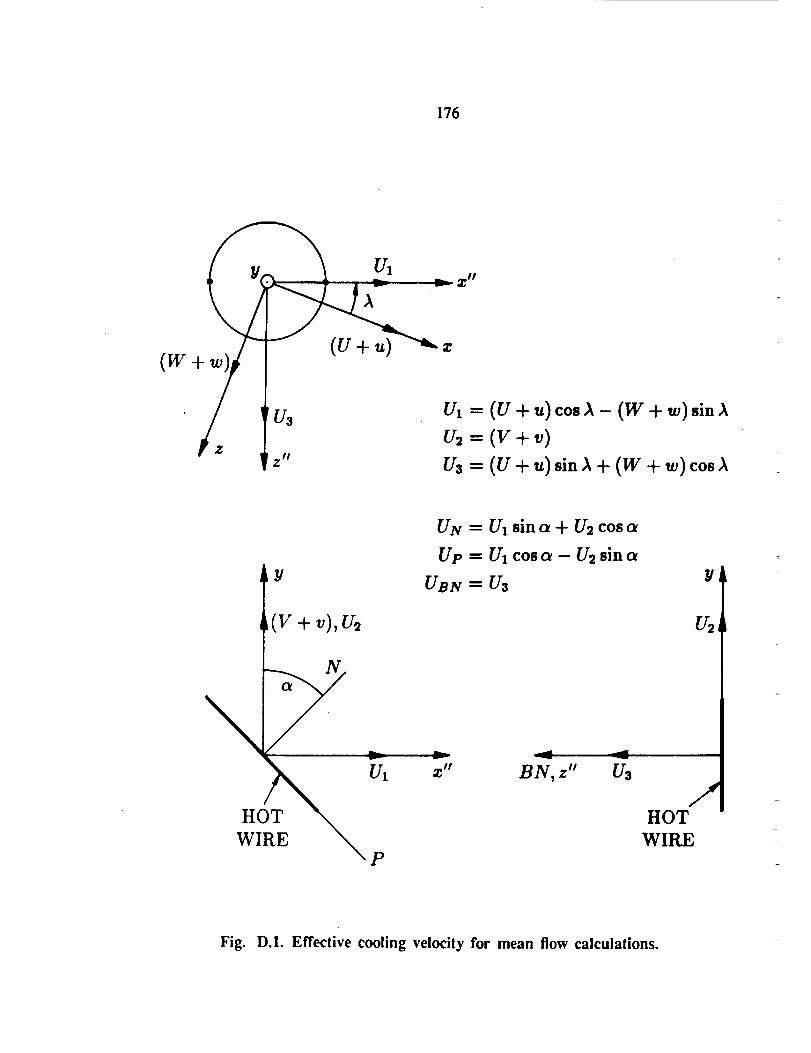
176
U1 _/t
A _ -
(w+
• / u_ v_ = (v + ,,)co_ _ - (w + _) _i,,;_v_ = (v + _)
z" Us = (I5 + u) sinA + (W + w) cos_
UN -- U1 sin a +/32 cos c_
Up = U1 cos c_ - U2 sin a
Y UBN=U3 Y
_(V+ v),U2
HOT _
WIRE _ P
z" B N, z"
U2
AHOT
WIRE
Fig. D.1. Effective cooling velocity for mean flow calculations.
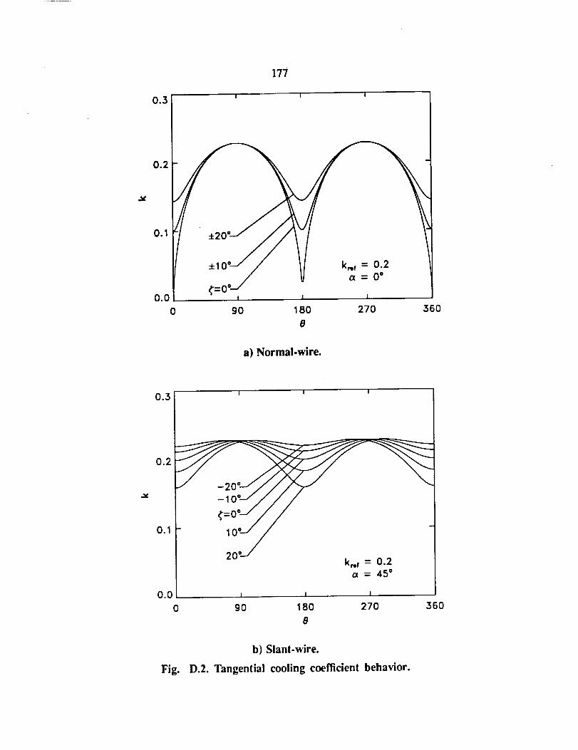
0.3
177
! I I
0.2
0.1
0 90 180 270 360
0
a) Normal-wire.
0.3
0.2
v
0.1
| I I
¢=°0--/_/ / I
",o.J/ t20"-,/
k,_ = 0.2a = 45 °
0.0 i i i
0 90 180 270 360
8
b) Slant-wire.
Fig. D.2. Tangential cooling coefficient behavior.

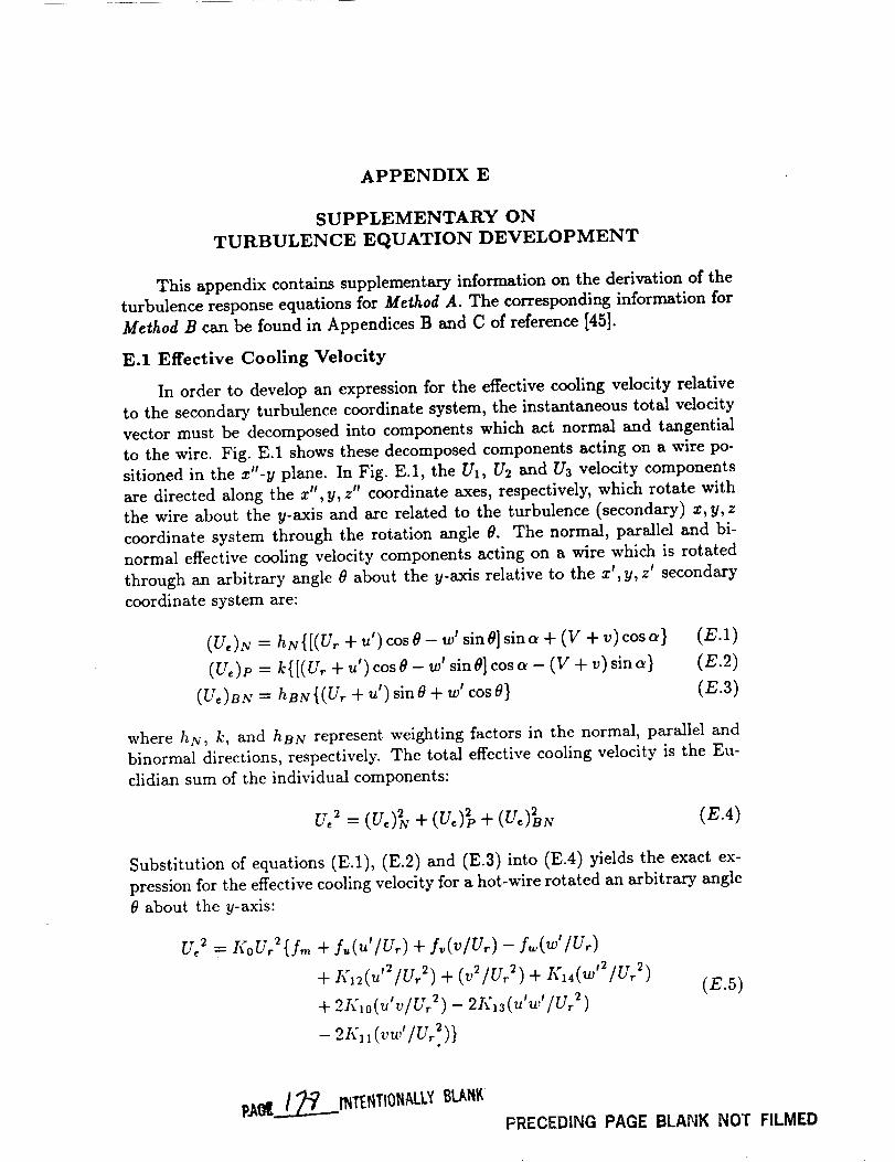
APPENDIX E
SUPPLEMENTARY ON
TURBULENCE EQUATION DEVELOPMENT
This appendix contains supplementary information on the derivation of the
turbulence response equations for Method A. The corresponding information for
Method B can be found in Appendices B and C of reference [45].
E.1 Effective Cooling Velocity
In order to develop an expression for the effective cooling velocity relative
to the secondary turbulence coordinate system, the instantaneous total velocity
vector must be decomposed into components which act normal and tangential
to the wire. Fig. E.1 shows these decomposed components acting on a wire po-
sitioned in the x'-y plane. In Fig. E.1, the U1, U2 and U3 velocity components
are directed along the x', y, z" coordinate axes, respectively, which rotate with
the wire about the y-axis and are related to the turbulence (secondary) x, y, z
coordinate system through the rotation angle 8. The normal, parallel and bi-
normal effective cooling velocity components acting on a wire which is rotated
through an arbitrary angle 0 about the y-axis relative to the x', y, z t secondary
coordinate system are:
(U,)N = hN{[(Ur + u') cos0- w' sin0] sina + (V + v) cosa} (E.1)(U,)p=k{[(Ur+u')cosO-w'sinO]cosa-(Y+v)sina) (E.2)
(Ue)BN= hBN{(Ur + u') sin8 + w' cosS} (E.3)
where hN, k, and hBN represent weighting factors in the normal, parallel and
binormal directions, respectively. The total effective cooling velocity is the Eu-
clidian sum of the individual components:
u,' = (u,)_ + (u,)_, + (u,)_N (E.4)
Substitution of equations (E.1), (E.2) and (E.3) into (E.4) yields the exact ex-
pression for the effective cooling velocity for a hot-wire rotated an arbitrary angle
0 about the y-axis:
ue_ = KoU?(fm + f,(_'/V,) + f,(v/Vr) - fw(w'/Vr)
+ K12(_'_/U,_)+ (_/U?) + I,'. (w''/Ur _)
+ 2Kao(u'v/U_ 2) - 2K13(u'w'/U,. 2)(=.5)
p,AOt_INTENTIONALLY BLANKPRECEDING PAGE BLANK NOT FILMED
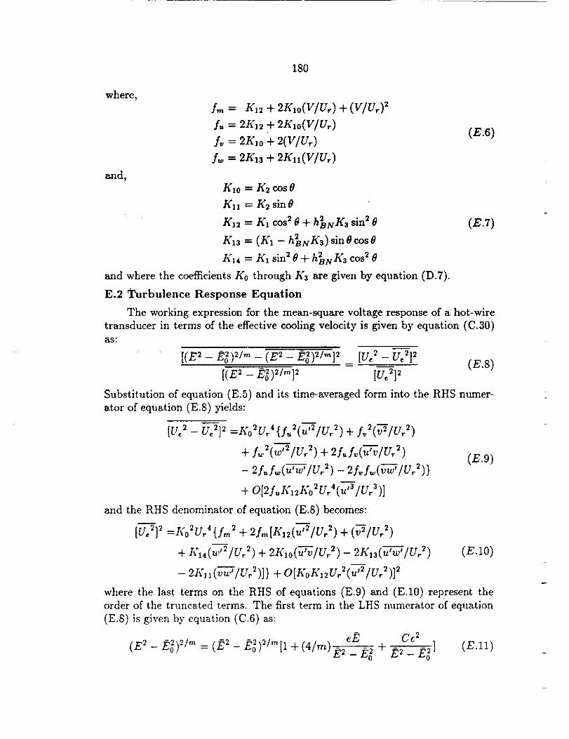
180
where,
Ba'Id_
fm= K_2+ 2K10(V/Ur)+ (Wur) _f. = 2K12 + 2K_o(V/U_)
y_ = 2K_o+ 2(v/u_)f,. = 2K13 + 2Kn(V/U,.)
(E.6)
K10 = K2 cos 8
Kn = K2 sin 8
Kn = K, cos 2 6 + h2BNK3 sin 2 8 (E.7)
K13 = (K1 - h_NK3) sin 0 cos O
K14 = K, sin 2 8 + h_NK3 cos 2 0
and where the coefficients K0 through K3 are given by equation (D.7).
E.2 Turbulence Response Equation
The working expression for the mean-square voltage response of a hot-wire
transducer in terms of the effective cooling velocity is given by equation (C.30)
as"
[(m - _o_)_/,--(e2 _ g,o_)2/,,,]_IV: _-TY]_= (E.8)
[(E2- g0_)_/m]_ [U_212
Substitution of equation (E.5) and itstime-averaged form into the RHS numer-
ator of equation (E.8) yields:
[u__- u_2]_=Ko2U/{fJ(,:IU__)+/J(-JIUJ)
+ fw2(w'21U"2) + 2f"f'_('_7_vlU"2) (E.9)
_ 2f,,f,,,(u-z_w,IU,.2) _ 2f,,f,.(-__IU,.2)}
+ O[2fj,'_2Ko_U,4(,,'_/U2)]
and the RHS denominator of equation (E.8) becomes:
[v.21_ =Ko2V/ {fro2+ 2:,.[l;_2(u,2/Vr2)+ (-J/V,?)
+ IQ4(w ,2/U,. 2) + 2IQo('Q-_v/U,. 2) - 2K13(u-Z'_w'/U,. 2) (E.10)
- 21<_(VJ'tu?)]} + O[KoK_UJ(,:IUJ)] _
where the last terms on the RHS of equations (E.9) and (E.10) represent the
order of the truncated terms. The first term in the LHS numerator of equation
(E.8) is given by equation (C.6) as:
c_ Cc2
(E_-[:o)_/_=(P_,_- £glW"[_+ (4/_)p:_ p_;°+ [:2_pj] (E._)
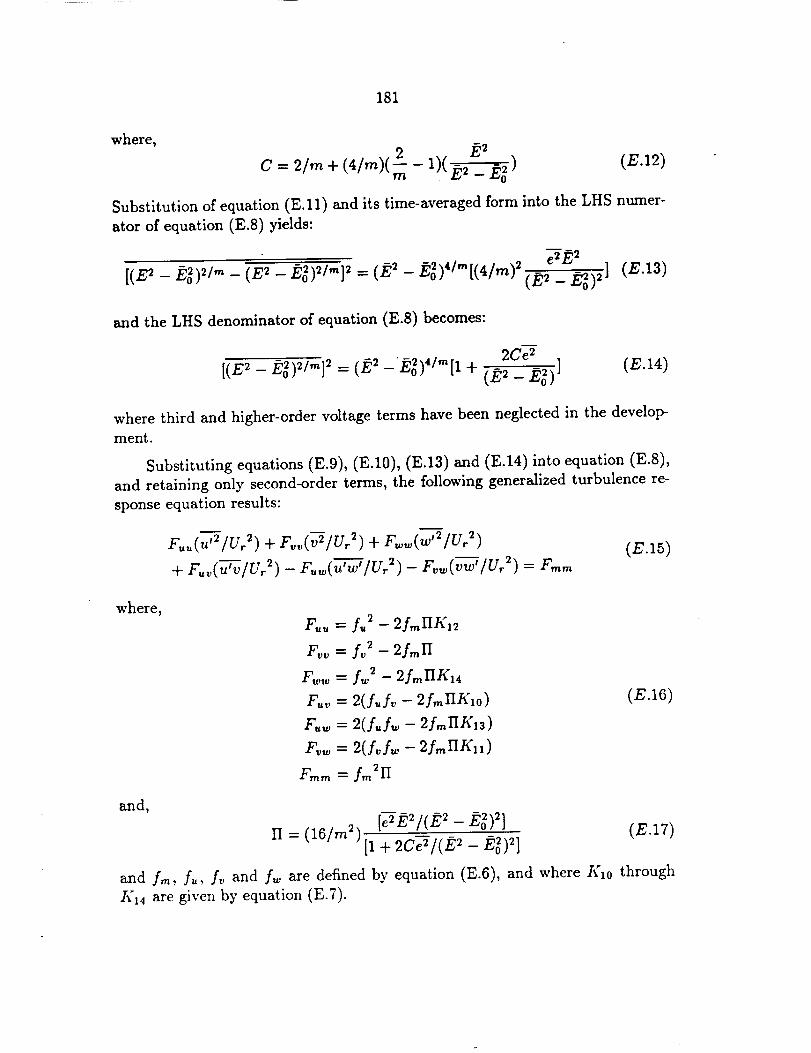
181
where,
c - 2/m + (4/.,)( - 1)(_:2_ _g ) (E.12)
Substitution of equation (E.11) and its time-averaged form into the LI-IS numer-
ator of equation (E.8) yields:
[(.m- _'o_)_/,,,-(E' - _g)'/',,]' = (._ - _o_)'/'[(4/m)_(_,__ _,_)_1_ (E._3)
and the LHS denominator of equation (E.8) becomes:
w
2Ce 2
[(E_- _o_1_/,,,1_= (._ -Eo_)"/"[1+ (._ _ ._o_1] (E.14)
where third and higher-order voltage terms have been neglected in the develop-
ment.
Substituting equations (E.9), (E.10), (E.13) and (E.14) into equation (E.8),
and retaining only second-order terms, the following generalized turbulence re-
sponse equation results:
w
F_(u'_/Vr _)+ F_(-_/Ur _)+ Fww(w'_/Vr2)
+ F_(-Y;_/Ur_)- F,w(_w--J_'/V,_)-F_.('_'/Vr _)= F_m(E.15)
where,
B_-'-Id _
F,,, = f2 _ 2fmIIK12
Fvv = fv2- 2fmII
Fww = f,,,2 _ 2f,,,IIK14
F.,_= 2(Af_ - 2fmlIKlo)
F._ = 2(]'jw - 2f, nlIKls)
F_w = 2(£fw - 2fmIIKll)
From = fm21"I
(E.16)
n = (16/m_) [_E_/(E_ - _g)2] (E.17)[1 + 2Ce"7/(E 2 - 2_02)2]
and fro, f,,, f_ and fw are defined by equation (E.6), and where Klo through
/(la are given by equation (E.7).
182
E.3 Algebraic Expression for "v"_/Ur 2
When slant-wire data taken at positions EA, FA, GA and HA are applied to
equation (E.15), the following four equations result:
( Fu_)EA (u'''_ /Ur 2) W (F,v)EA (v'_/Ur 2)
+ (Fww)EA (W '''TIUr 2 ) + (FIv)EA (u-_v/Ur 2) (E.18)
-- (F.w)EA (u-7_wl/Ur2)- (Fvw)EA (_/Ur 2) = (F.m)EA
(F..)F. (u'--T/V2) + (n,)F, (V/U2)
+ (Fww)FA (-_i/Ur2) + (F.v)FA ('uT_v/Ur2) (E.19)
- (F._)F_(_--_'/V_2)- (nw)F_ (-_'/U2) = (F.._.)F_
(F..)G.(_'-_IU_2)+ (F_)G_(VIU,2)
+ (fww)GA (w'_/Ur _ ) + (Fuv)GA (¥'vv/Ur 2 ) (E.20)
- (F..)c. (_-r'J'/Vr2)- (F_.)G. ('_'-_'/V_2)= (F._m)G.
(r,,)Ha(U'2/V_ 2) + (F,,_)HA(-_IU_ 2)
+ (F,w)HA(W,"'T/U2) + (F,_)HA(-_'_v/U2) (E.21)
- (F._)H_(VJ'/U_2) _ (F_w),_('_'/V. _) = (F..)H,
where the expressions for Fuu,...F_,w are given by equation (E.16). Subtraction of
equation (E.21) from (E.18) and (E.20) from (E.19) yields the following combined
equations:
[(F,,)E_ -- (F.,)HA](u'2/V_ 2) + [(F_)EA -- (Fw)HA](-_IU_ 2)
+ [(Fw_)EA - (Fww)HAl('w'2/U, ?) + [(F,,,)EA - (Fuv)HA](-_'_v/U_ 2)
- [(F,_)E, - (F.w)._ ](_-_'/v, 2) - [(Fvw)EA -- (Frw)HA](v-_wt/Ur 2)
= [(F_)E_ - (F_),_]
[(E..)F_- (F..)G_I(,'-_/U.2)+ [(n.)r_- (F_)a_](V/U__)
+ [(Fww)FA -- (Fww)GA](w'21Ur 2) + [(Fuv)FA -- (F.v)GA](_vlUr 2)
-- [(F_,u,)FA -- (Fuw)a,l(u-_wtlUr 2) -- [(Frw)FA -- (Fvw)aA](-_wr/Ur 2)
(E.22)
(E.23)
Multiplication of equation (E.22) by [(F,,w)FA - (F,,w)cA] and equation (E.23)
by [(F=,_)E_ -- (F,w)H,] and subtraction of the resulting equations yields:
(s,._ - s_..)(_'--_IU.2)+ (s,_ - s_)(-#IU. _)
+ (s,,,_,- s_w)(_,'_lU?) + (s,._ - s_._)(-_lU, _) (E.24)
- (s,,,_,- s_,_,)(-C-_'lU,_)= (s,_.. - S_mm)
183
where,
(i,j = u,v,w,m)
(/J)E. =(/J)H.
(fufv)Ea =(fury)HA
(f,,fw)Ea = --(f,,fw)Ha
(Afw)_,.,= -(f,,L,,)..,
(K,o)E.,= (I':_o)._
(zt'_3)_:A= -(1¢13)._(K14)EA= (K,4)..
; (A2)F. = (A2)a_
; (L_)F,, = (f2)G.,
; (f,,?)F., = (.:,2)G.,
; (AJ)FA = (f.?)G_
; (Lf,,)r.,= (f,,f.)o,,
; (f,,fw)Fa = -(f,,f,,,)Ga; (fvfw)FA----(fvfw)GA
; (K_o)r_ = (g,o)o_; (K.)F.=--(K_)G_
; (K13)Fa=-(A'a3)aa
; (K_4)F. = (K_4)o.,
(E.25.a)
(E.25._)
By imposing conditions (E.25.a) and (E.25.b) on equation (E.24), the following
final form is obtained:
(_ I;_.E. - _2I;_2.r_)(_'2/v_ _) + (_ - _2)(V /v_2)+
(E.26)where
s_= -S[(Afw)F_- (fmK_3)F_(nr_+ nG_)](nE.- n..)(f.,)_
and,
6",_,_= 16[(A/,.)F., - Ixhs,FA(f,.)F,, (nF,, + nc,,)]x[(A:,.,)E., - K,_,t:,,(J,_)E,,(nt:,,+ nil,,)]
S_,,,.,= 16[(/_,/,,,)EA--I(_,E.,(I,,,)E.,(nE.,+ IlH._)]x[(Lfw)Fa - I(,,,va (/,-.)F,_(IIFA+ IIo.)]
and,
By observing the behavior of the coefficients f,,, f_,, f_, fro, K_o, 1"£11, Kn, K_
and K_4 at positions EA, FA, GA and HA, it can be shown that:

184
and where the expression for II is given by equation (E.17). An algebraic ex-
pression for vw', applicable to low turbulence intensity flows, can be derived
from equation (E.24) in a similar manner; however, it can also be extracted as
a special case from equation (E.24) by substituting F, = f_fi; (i - u, v, w),
F_i = 2fifi; (i,j = u,v,w; i # j) and Fm_n = f,,2_ into equation (E.24),
which yields:
S1,,,, = $1,,,, = 51,,,_ = S_,,,, = 0
$2,,,, = S_,,,, = $2,,,,,, = $2,,_ = 0
and_
S,,,w = [2(Af,,,)FA -- 2(A f,_)GA][2(Afw)EA -- 2(Af.)HA]
=(4Afw)FA(4Af_)EA
Slmm "_- (4/u/w)F_ (fro 2)EA (_EA -- 7rHA)
S mm= (:m2)F ( FA-- GA)
Substitution of these coefficients back into (E.24) yields, after some rearrange-
ment:
Vr 2 w (2f,,.fw)FA (2f,,fw)EA -- (2f,,f,,,)EA (2f,_f,,,)FA
(E.27)
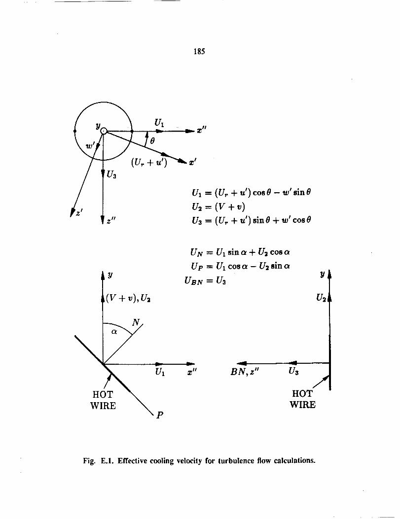
185
_ _ Z te
UI = (U,,+ u')cosO - w' sinO
Us
/_, u,.= (v+_)z" Us = (U,. + u') sinO + w' cosO
_Y
_(v + v),u2
WIRE _ P
UN = UI sin a + U2 cos c_
Up = UI cos c_ - U_ sin a
UBN=U3
B__tl Z H
Y
U2
/1HOT
WIRE
Fig. E.I. Effective cooling velocity for turbulence flow calculations.
APPENDIX F
VERIFICATION OF THE HOT-WIRE TECHNIQUE
The low-intensity form of the Method A hot-wire technique proposed in
the Appendix C has been partially verified by means of measurements in fully-
developed turbulent pipe flow under simulated skewed flow conditions. In addi-
tion, the implementation of the Method B technique into the present study was
verified in pipe flow for the unskewed case. The pipe flow facility, as well as the
full verification procedure for Method B, is described in detail in references [45]
and [47].
F.1 Fully-developed pipe flow
A schematic of the pipe flow verification setup for Method A is shown in
Fig. F.1. The probes axe inserted into the ftow through a slot (6.5 x 13 mm)
located one diameter upstream from the pipe exit. The outside edges of the
slot were chamfered to allow the probe to be skewed 4-20 degrees in the pitch
direction. The verification measurements were made on the far side of the pipe to
minimize disturbances due to the slot. The diameter of the pipe is 10.16 cm and
all the verification measurements were made at an operating Reynolds number of
125,000 based on the centerline velocity and the pipe diameter. The development
length for the pipe flow is L/D = 136.
Along a radial traverse of turbulent pipe flow, azimuthal symmetry imposes
the condition that the _ and the _ Reynolds stress components (relative to
pipe flow coordinates) are identically zero. When the flow is fully-developed, the
u--'_shear stress component, when normalized by the friction velocity, is a linear
function of the radial location if the very near-wall region is excluded i.e.,:
t/U r
_ (F.1)R
where the friction velocity is given as:
= (F.2)
and Ub (bulk velocity) and f (friction factor) are determined from:
1/V7 = 2.01og,0(n vq) - 0.s
with,
UdUd = Reb/Re_l
Red = UdD/u
P,A(_____._IN TENTIONALLY BLANK
PRECEDING PAGE BLANK NOT FILMED
188
and where the Reynolds number ratio is given by a correlation proposed by
Eppich [40]:
Reb/Red = 0.045 log10 (Rect)+ 0.600
For the present study, the friction velocity was calculated from equation (F.2)
and also measured independently with a Preston tube using the calibration given
by equation (3.3). The results from the two methods were virtually the same:
U,/Ub = 0.04726 @ Re¢t= 125,000
F.2 Verification approach
Since, for low intensity flows, the yaw angle 7 (refer to Fig. C.2.a) can be
determined with sufficient accuracy by hulling of a two-tube Conrad probe or by
the normal hot-wire nuUing technique described by Page [62], the low intensity
verification procedure for Method A was initially performed for unknown pitch
angles _ only. For this case, the transverse velocity component W is zero and
the primary (mean flow) coordinates and secondary (turbulence) coordinates
coincide (see Fig. C.3.a). Wire Positions 1,2,3 and 4 in the primary coordinate
system (see Fig. C.2), then, are equivalent to wire Positions A, B, CA and DA in
the secondary coordinate system, respectively. For the following discussion, the
probe rotation angle will be denoted by 8 and the prime (i) superscript associated
with the secondary (turbulence) coordinate system will be dropped. The probe
rotation angle 8 is defined as shown in Fig. F.2.
The proposed procedure for determining the mean velocity components and
Reynolds stress components is presented in detail in Appendix C and is summa-
rized here. The V/U and W/U mean velocity ratios are determined by applying
data obtained with the offset prong slant-wire probe (Fig. C.l.b) at positions
8 = 0 and 180 ° and normal-wire data obtained at 8 = 225 and 315 ° to equation
(C.14). Once the mean velocity-ratios are known, the axial velocity component
U is evaluated at wire Position 1 by means of equation (C.16), and it's equiv-
alent for wire Positions 2,3 and 4, and then the four values are averaged. The
procedure for determining the components of the Reynolds stress tensor is as
follows:
1) u2,v2,_-_ - Data obtained with a normal-wire at 8 = 270 ° and with the offset
prong slant-wire configuration (Fig. C.l.b) at 8 = 0 and 180 °, when applied
to equation__C.36), results in a 3 x 3 system of equations which, when solved,
yields the u 2 ,v 2 and _-fi Reynolds stress components.
2) _ - Data obtained with the straight prong slant-wire probe (Fig. C.l.c)
at 8 = 45,135,225 and 315 °, when applied to equation (C.41), yields an
algebraic expression for the _ stress component.
189
3) w2,_-'_ - Normal-wire data obtained at 0=225 and 315 ° and the stress com-
ponents from 1) and 2) above, when applied to equation (C.36), results in a
2 x 2 system of equations which, when solved, yields the w 2 and _ Reynolds
stress components.
By considering pitch skewness only in the fully-developed pipe flow verification,
the _ and 9-'_.__stress components are identically zero regardless of the pitch angle.
Further, the w 2 stress component is invariant as the pitch angle is changed.
F.3 Hot-wlre probe design and construction
The proposed Me_hod A hot-wire technique requires the sequential use of
two and possibly three probe configurations which are illustrated in Fig. C.I.
All the probes for the Method A technique were constructed from scratch with
the basic dimensions and materials as shown in Fig. F.3. Detail dimensions of
the probe prongs for the three probe configurations are shown in Fig. F.4. One
of the constraints imposed on the probe design was that it had to fit through a
4.57 mm (0.180 in) access hole which corresponds to the diameter of a standard
Thermal Systems Inc. (TSI) probe holder. This constraint places a limitation on
the amount of offset that can be applied to a probe such as the slant-wire probe
shown in Fig. F.4.b. Given a diameter that the probe must pass through without
interference, a compromise must be made between probe offset and the distance
between the probe prong tips (hot-wire length).
F.4 Calibration
The hot-wire probes were calibrated in the core flow at Data Station 1 of
the transition duct flow facility (see Fig. 3.2). A PiLot tube placed adjacent
to the hot-wire probe and the local wall static pressure provided a reference
calibration velocity. The normal-wire was calibrated in the 8 -- 270 ° position
and the straight prong slant-wire was calibrated in the 0 = 0 ° position. The
offset prong slant-wire was calibrated in both the 0 = 0 and 180 ° positions. A
typical plot of an offset prong slant-wire probe calibration is shown in Fig. F.5.
Clearly, the calibrations are not equivalent. There are two possible reasons for
the differences. First, unlike Melhod B where, for unskewed flow, the stagnation
line for the normal velocity component on the hot-wire is unchanged regardless of
rotational position, for Method A the stagnation line rotates around the hot-wire
as the probe is rotated. Waviness or other imperfections in the wire may cause it
to respond differently when the flow is exposed to the front or back "side" of the
wire. The second cause is the influence of the upstream probe prong when the
wire is in the 8 = 180 ° position. There are indications that the latter cause is
responsible for the discrepancy. If wire imperfections were responsible, then the
calibration curves should vary randomly with each different wire. Calibration
with separate but similar probes and several different wires has shown that the
190
calibration curve for Position B (8 = 180°) consistently rides slightly higher then
the curve for Position A. If it is assumed that the wire is exposed to the true
calibration velocity when in Position A and that the wire itself is perfect, that
is, it will respond the same in any orientation so long as the effective cooling
velocity remains constant, then Fig. F.5 indicates that the wire is exposed to a
higher velocity when in Position B than when in Position A. It is plausible that
the higher velocity in Position B is a result of the local acceleration of the flow
as it is displaced about the upstream probe prong. This behavior is illustrated
in Fig. F.6.
The question arises as to whether the prong influence is significant enough to
preclude accurate flow measurements. The effect of different calibration slopes in
the # = 0 and 180 ° positions can be taken into account in the mean flow response
equations by replacing equation (C.7.a) by:
_,,2 = (B2/B,)2/m(_,/S2) (F.1)
and by using the appropriate value of B in equation (C.16) or its equivalent for
wire Position 2. The turbulence response equations are unchanged since they
are cast into a non-dimensional form in which the calibration slope is eliminated
(see equation (C.25)). By accounting for the different calibration characteris-
tics of the offset slant-wire, it should be possible to obtain accurate mean flow
and turbulence data for unskewed flow conditions (V=W=O). The effect of the
probe prong interference under skewed conditions is uncertain and requires fur-
ther study.
F.5 Unskewed flow verification
The mean velocity and Reynolds stress components in the fully-developed
pipe flow were measured by means of the Method A and Method B hot-wire
techniques. The measurements by the Method B technique were performed to
demonstrate proper operation of the data acquisition equipment and correct pro-
gramming of the response equations. For the Method A measurements, the offset
slant-wire data were reduced using the calibration in Position A only (uncor-
rected) and also using the calibration in Positions A and B (corrected) as de-
scribed in the previous section. The measured axial mean velocity profile and
transverse flow angles are shown in Fig. F.7.a and Fig. F.7.b, respectively. In
Fig. F.7.a, a reference velocity distribution measured with a flattened Pitot probe
is shown for comparison. The axial velocity results for Method A were calcu-
lated from the output of the slant-wire only, rather then averaging the slant and
normal-wire results, in order to illustrate more clearly the effect of the calibra-
tion anomaly. The corrected Method A results and the Method B results show
very good agreement with the reference distributions. The uncorrected Method
A results show the need to include the calibration of the offset prong slant-wire
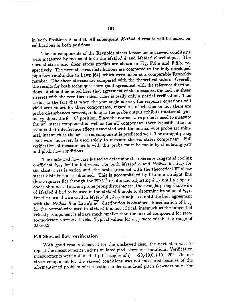
191
in both Positions A and B. All subsequent Method A results will be based on
calibrations in both positions.
The six components of the Reynolds stress tensor for unskewed conditions
were measured by means of both the Method A and Method B techniques. The
normal stress and shear stress profiles are shown in Fig. F.8.a and F.8.b, re-
spectively. The normal stress distributions are compared to the fully-developed
pipe flow results due to Lawn [64], which were taken at a comparable Reynolds
number. The shear stresses are compared with the theoretical values. Overall,
the results for both techniques show good agreement with the reference distribu-
tions. It should be noted here that agreement of the measured _ and _ shear
stresses with the zero theoretical value is really only a partial verification. This
is due to the fact that when the yaw angle is zero, the response equations will
yield zero values for these components, regardless of whether or not there are
probe disturbances present, so long as the probe output exhibits rotational sym-
metry__about the 8 = 0 ° position. Since the normal-wire probe is used to measure
the w 2 stress component as well as the _ component, there is justification to
assume that interference effects associated with the normal-wire probe are mini-
mal, inasmuch as the w _ stress component is predicted well. The straight prong
slant-wire, however, is used solely to measure the _ stress component. Full
verification of measurements with this probe must be made by simulating yaw
and pitch flow conditions.
The unskewed flow case is used to determine the reference tangential cooling
coefficient krel for the hot-wires. For both Method A and Method B , krel for
the slant-wires is varied until the best agreement with the theoretical h-_ shear
stress distribution is obtained. This is accomplished by fitting a straight line
(least-squares fit) through the _--6/U 2 results and adjusting kr,l until a slope of
one is obtained. To avoid probe prong disturbances, the straight prong slant-wire
of Method A had to be used in the Method B mode to determine its value of kr, f.
For the normal-wire used in Method A, kre! is adjusted until the best agreement
with the Method B or Lawn's w 2 distribution is obtained. Specification of k_ I
for the normal-wire used in Method B is not critical, inasmuch as the tangential
velocity component is always much smaller than the normal component for zero-
to-moderate skewness levels. Typical values for kreI were within the range of0.05-0.2.
F.6 Skewed flow verification
With good results achieved for the unskewed case, the next step was to
repeat the measurements under simulated pitch skewness conditions. Verification
measurements were obtained at pitch angles of ( = -20,-10,0,+10,+20 °. The
stress component for the skewed conditions was not measured because of the
aformentioned problem of verification under simulated pitch skewness only. For
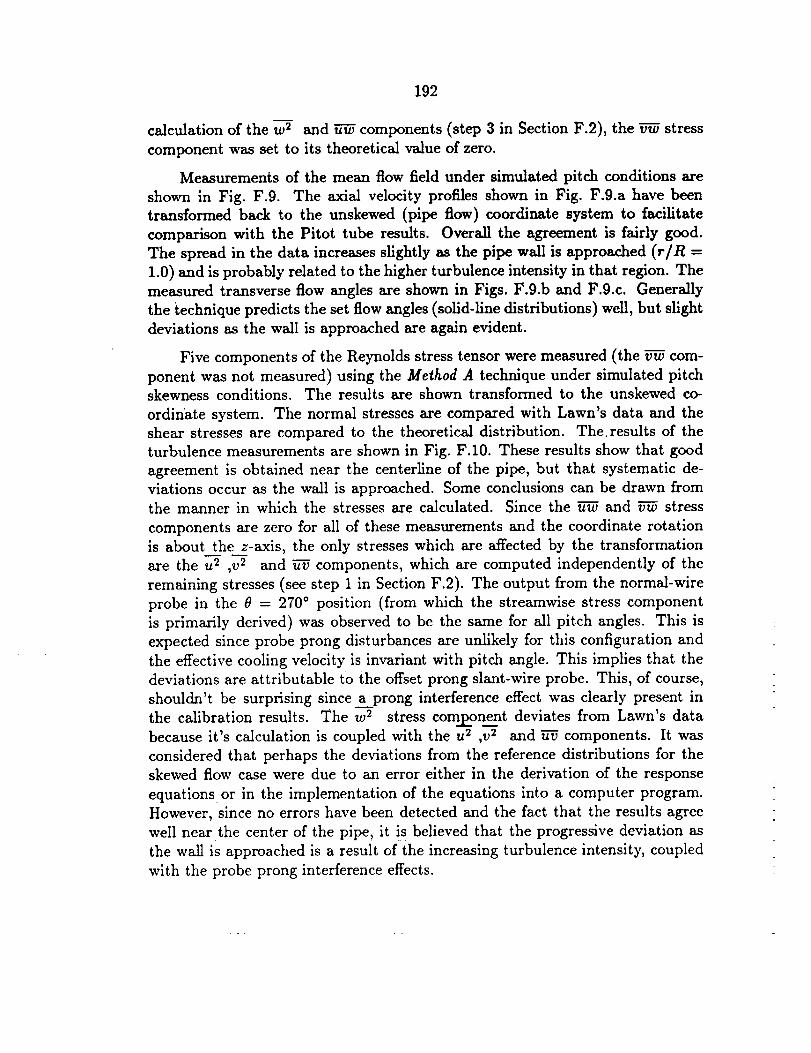
192
m
calculationof the w 2 and _ components (step 3 in Section F.2),the _ stress
component was set to itstheoreticalvalue of zero.
Measurements of the mean flow fieldunder simulated pitch conditions are
shown in Fig. F.9. The axial velocity profilesshown in Fig. F.9.a have been
transformed back to the unskewed (pipe flow) coordinate system to facilitate
comparison with the Pitot tube results. Overall the agreement isfairlygood.
The spread in the data increasesslightlyas the pipe wall isapproached (r/R =
1.0)and isprobably relatedto the higher turbulence intensityin that region. The
measured transverse flow angles are shown in Figs. F.9.b and F.9.c. Generally
the technique predicts the set flow angles (solid-linedistributions)well,but slight
deviations as the wall isapproached are again evident.
Five components of the Reynolds stresstensor were measured (the _ com-
ponent was not measured) using the Meihod A technique under simulated pitch
skewness conditions. The results are shown transformed to the unskewed co-
ordinate system. The normal stressesare compared with Lawn's data and the
shear stressesare compared to the theoreticaldistribution. The.results of the
turbulence measurements are shown in Fig. F.10. These resultsshow that good
agreement is obtained near the centerlineof the pipe, but that systematic de-
viations occur as the wall isapproached. Some conclusions can be drawn from
the manner in which the stressesare calculated. Since the ff-_and _ stress
components are zero for allof these measurements and the coordinate rotation
is about t___hez-axis,the only stresseswhich are affected by the transformation
are the u2 ,v2 and _'V components, which are computed independently of the
remaining stresses(see step I in Section F.2). The output from the normal-wire
probe in the 8 = 270 ° position (from which the strearnwise stresscomponent
is primarily derived) was observed to be the same for allpitch angles. This is
expected since probe prong disturbances are unlikely for this configuration and
thc effectivecooling velocity isinvariantwith pitch angle. This implies that the
deviations are attributableto the offsetprong slant-wireprobe. This, of course,
shouldn't be surprising since a.__pronginterferenceeffectwas clearlypresent in
the calibrationresults. The w 2 stresscom_p_one...ntdeviates from Lawn's data
because it'scalculationis coupled with the u2 ,v2 and _'_components. It was
considered that perhaps the deviations from the reference distributionsfor the
skewed flow case were due to an error either in the derivation of the response
equations or in the implementation of the equations into a computer program.
However, since no errorshave been detected and the fact that the resultsagree
well near the center of the pipe, itisbelieved that the progressive deviation as
the wall is approached is a resultof the increasing turbulence intensity,coupled
with the probe prong interferenceeffects.
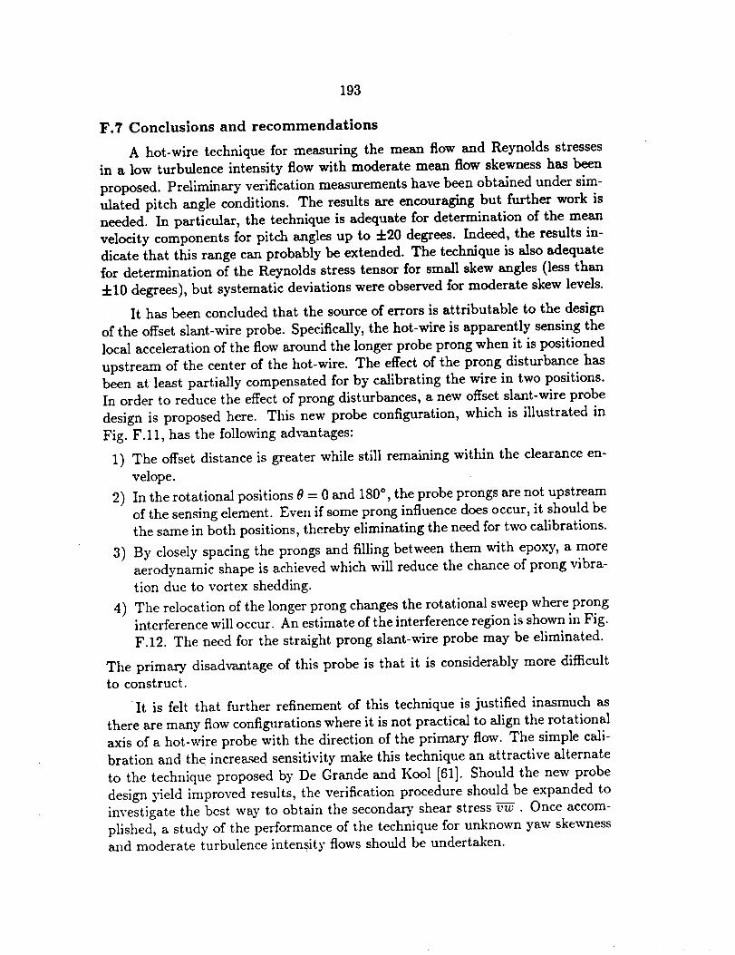
193
F.7 Conclusions and recommendations
A hot-wire technique for measuring the mean flow and Reynolds stresses
in a low turbulence intensity flow with moderate mean flow skewness has been
proposed. Preliminary verification measurements have been obtained under sim-
dated pitch angle conditions. The results are encouraging but further work is
needed. In particular, the technique is adequate for determination of the mean
velocity components for pitch angles up to 4-20 degrees. Indeed, the results in-
dicate that this range can probably be extended. The technique is also adequate
for determination of the Reynolds stress tensor for small skew angles (less than
4-10 degrees), but systematic deviations were observed for moderate skew levels.
It has been concluded that the source of errors is attributable to the design
of the offset slant-wire probe. Specifically, the hot-wire is apparently sensing the
local acceleration of the flow around the longer probe prong when it is positioned
upstream of the center of the hot-wire. The effect of the prong disturbance has
been at least partially compensated for by calibrating the wire in two positions.
In order to reduce the effect of prong disturbances, a new offset slant-wire probe
design is proposed here. This new probe configuration, which is illustrated in
Fig. F.11, has the following advantages:
1) The offset distance is greater while still remaining within the clearance en-
velope.
2) In the rotational positions _ = 0 and 180 °, the probe prongs are not upstream
of the sensing element. Even if some prong influence does occur, it should be
the same in both positions, thereby eliminating the need for two calibrations.
3) By closely spacing the prongs and filling between them with epoxy, a more
aerodynamic shape is achieved which will reduce the chance of prong vibra-
tion due to vortex shedding.
4) The relocation of the longer prong changes the rotational sweep where prong
interference will occur. An estimate of the interference region is shown in Fig.
F.12. The need for the straight prong slant-wire probe may be eliminated.
The primary disadvantage of this probe is that it is considerably more difficult
to construct.
It is felt that further refinement of this technique is justified inasmuch as
there are many flow configurations where it is not practical to align the rotational
axis of a hot-wire probe with the direction of the primary flow. The simple cali-
bration and the increased sensitivity make this technique an attractive alternate
to the technique proposed by De Grande and Kool [61]. Should the new probe
design yield improved results, the verification procedure should be expanded to
investigate the best way to obtain the secondary shear stress v---_. Once accom-
plished, a study of the performance of the technique for unknown yaw skewness
and moderate turbulence intensity flows should be undertaken.
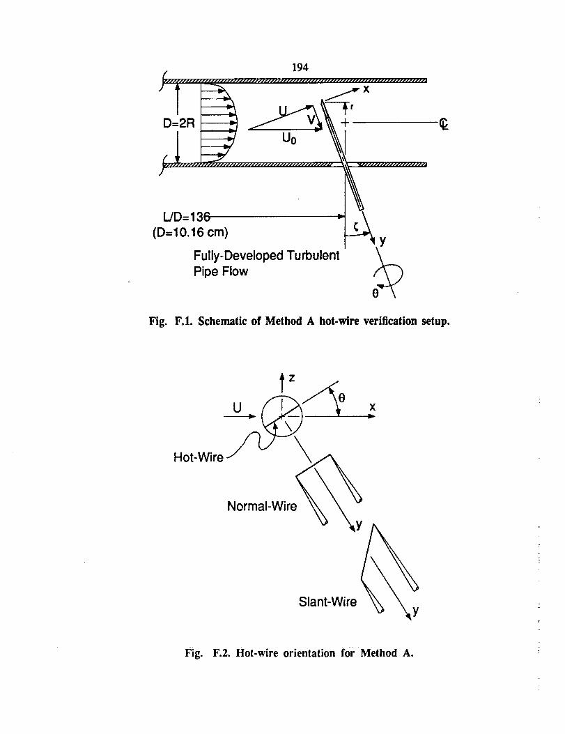
194_JJJJlllJi_ _i.¢lJJJf.cJliflJ.,,'l_11_'_
' _._x
(D=I 6era)
Fully-Developed TurbulentPipe Flow
Fig. F.1. Schematic of Method A hot-wire verification setup.
Normal-Wire_y
Slant-Wire
X
Fig. F.2. Hot-wire orientation for Method A.
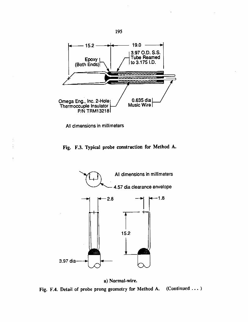
195
= 15.2 =-_ 19.0
/ 3.97 O.D.S.S. I
Epoxy 7 I D(Both Ends) to 3.1 5 . .
.. ..,.,.,.,._,-_+..'..'-.".'__ .....
/
Omega Eng', Inc. 2-Holel / 0.635 dia
Thermoeouple Insulator [----/ Music WireP/N TRM13218
All dimensions in millimeters
Fig. F.3. Typical probe construction for Method A.
-+-
i3.97 dia---=-_
All dimensions in millimeters
)'_'- 4.57 dia clearance envelope
.*--2.8
4--
15.2
a) Normal.wire.
Fig. F.4. Detail of probe prong geometry for Method A. (Continued ... )
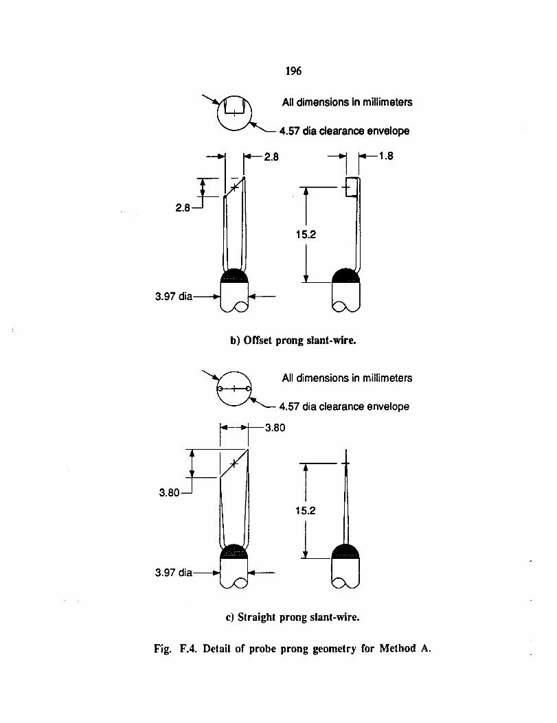
196
All dimensions in millimeters\
--t-
_"'--- 4.57 dia clearance envelope
3.97 dia-_--_.,,<
'_--2.8
4--
b) Offset prong slant-wire.
3.97 dia-_---_
X
.,,<
All dimensions in millimeters
4.57 dia clearance envelope
--3.80
T15.2
c) Straight prong slant-wire.
Fig. F.4. Detail of probe prong geometry for Method A.
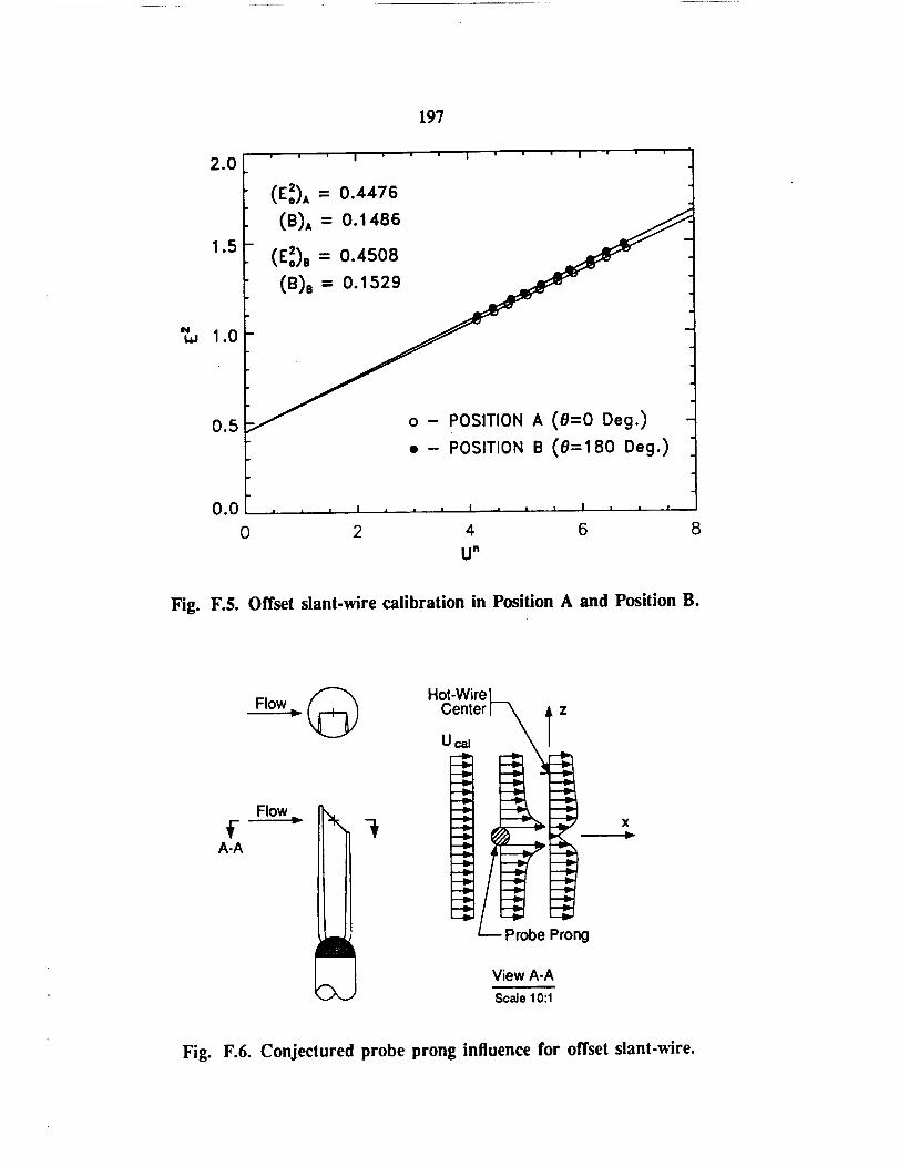
197
2.0
1.5
_._ 1.0
0.5
' ' ' I " ' ' | ' ' ' I • ' '
(E=Z)A = 0.4476
(B)A = 0.1486 __
(E:),: o.4so8 "
- o - POSITION A (8=0 Deg.)
• - POSITION B (0=180 Deg.)
0.0 , = _ I , , , 1 _ , , I _ , =
0 2 4 6 8
U"
Fig. F.5. Offset slant-wire calibration in Position A and Position B.
Flowf
A-A
II
Hot-Wire I_
Center I_ fzU_
g
View A-A
Scale 10:1
Fig. F.6. Conjectured probe prong influence for offset slant-wire.
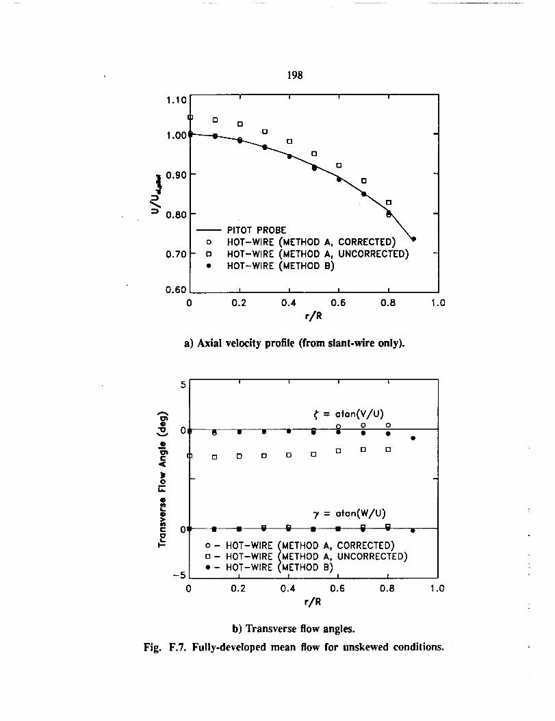
198
1.10
1,00
0.90
0.80
0.70
I I l I
00
.0
0
- PITOT PROBE
o HOT-WIRE (METHOD A, CORRECTED)D HOT-WIRE (METHOD A, UNCORRECTED)
• HOT-WIRE (METHOD B)
0.601 , l m J
0 0.2 0.4 0.6 0.8
r/R
a) Axial velocity profile (from slant-wire only).
.0
Q
e
t-
oikt.
0
k.
Q>,me-
Ep-
Fig.
5
O(
O:
I I I I
0 0 [] []
¢ = olo.(vlu)S _ o o
[] 0 0 []
7 = o'fon(W/U)
__ m ¢3 I_ m m r'l []m W v w m w W v
o- HOT-WIRE (_METHOD A, CORRECTED)o HOT-WIRE (,METHOD A, UNCORRECTED)
•- HOT-WIRE (METHOD B)-5 .... i m.... m =
0 0.2 0.4. 0.6 0.8 1.0
r'/R
b) Transverse flow angles.
F.7. Fully-developed mean flow for unskewed conditions.
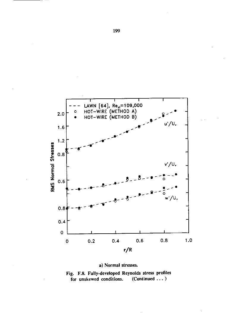
199
Q
m
tt_
tw
2.0
1.6
1.2
0.8
0.6
0.8
0.4
0
I I I
LAWN [64], Re=,=109,OOO
_ o HOT-WIRE (METHOD A) .. •
• HOT-WIRE (METHOD B) .-_ "
..f'
,F
.-e"
t
u'/U,
v'/U,.m
L - -0- - --.e"- -
m
.8_--8--
F - -8" -
w'/UT
0
I I I I
0.2 0.4 0.6 0.8
r/R
1.0
a) Normal stresses.
Fig. F.8. Fully-developed Reynolds stress profiles
for unskewed conditions. (Continued...)
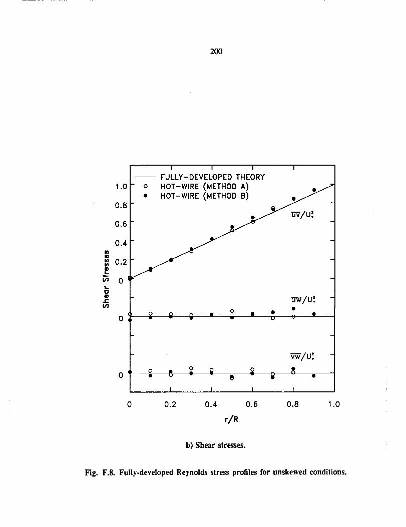
2OO
@
II
P,4--
(/1
I.00
t/1
1.0
0.8
0.6
0.4
0.2
0
0
0
I I I I
FULLY-DEVELOPED THEORY
- o HOT-WIRE (METHOD A) ,_-'_
_ • HOT-WIRE (METHOD B) _ _
- w/u:
, _ £ g ,, o • • "• 0 v
0
0 • 0 Q Q
• u - $ ¥
I ...... I I
0.2 0.4 0.6
r/R
_--_/u; -
8
!
0.8 I .0
b) Shear stresses.
Fig. F.8. Fully-developed Reynolds stress profiles for unskewed conditions.
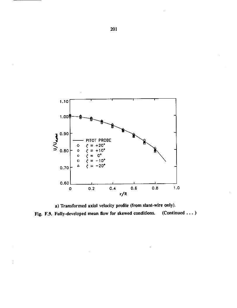
201
1.10
1.001
0.90
0.80
0.70
I I I I
0 ¢ = +20 = '-'- o ¢ = +10= _,
o ¢= 0= \D ¢ = -10=
_ ,_ ¢ = -20 °
0.60 , , I 10 0.2 0.4 0.6 0.8
r/R.0
a) Transformed axial velocity profile (from slant-wire only).
Fig. F.9. Fully-developed mean flow for skewed conditions. (Continued ... )
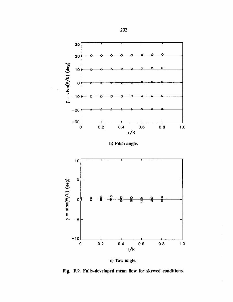
202
O_@
"oV
:D
t-O
,mira
0
II
av,
30
20
10
0
-10_
-20 '-
-30
0
A= v
I I I I
v v _, _ - -
m M _ _ _ _ n
A A A ,_. A A A
I l I I
0.2 0.4 0.6 0.8
r/R
b) Pitch angle.
.0
10
O_@
"10U
ot-U
U
II
t'- -5
I I l I
-10 i i i i
0 0.2 0.4 0.6 0.8 1.0
r/R
c) Yaw angle.
Fig. F.9. Fully-developed mean flow for skewed conditions.
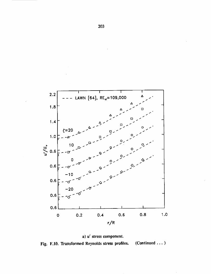
203
2.2
1.8
1.4
1.0
I-
:3
>. 0.6
0.6
0.6
0.6
0.6
I I I
LAWN [64], RE©,=109,000
f=20
T
I0O. 4
.p
,.,
-10 ..--0_
_--o"
-20 ..
_- - -<>'-
2%, _-
,i
.s"
0
["_ j t
[] /" 0./
O-" 0.."j.
o-
9" 0
O_ _"
/ @/
_'_ 9"
9"
I I I
0 0.2 0.4 0.6
r/R
I
j"
o"
D
s"
J
J
I
0.8 1.0
a) u' stress component.
Fig. F.IO. Transformed Reynolds stress profiles. (Continued ... )
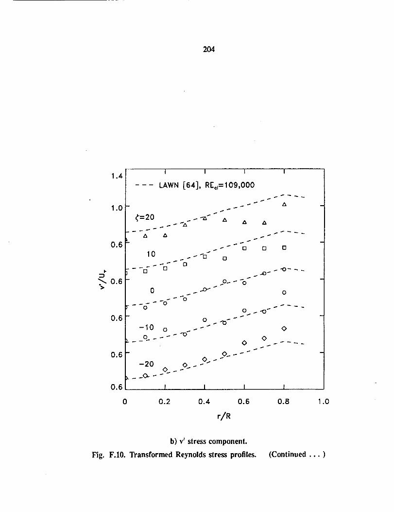
204
1.4
1.0
0.6
I-
._ 0.6
0.6
0.6
0.6
i I I i
LAWN [64], RE=,=109,000
¢=20
L
10
r'l
... s
0_.--0 _
0
-10 o -'o"
s ...0.--
s
..., -," []
13
.,..,
s
s..O _
o_ --- %
0 .,. -,O _
o .- ."o-s
<>
m
-20 O_ -0""
! I ........ !
[] []
0
<>
0 0.2 0.4 0.6 0.8 1.0
r/R
b) v' stress component.
Fig. F.10. Transformed Reynolds stress profiles. (Continued ... )
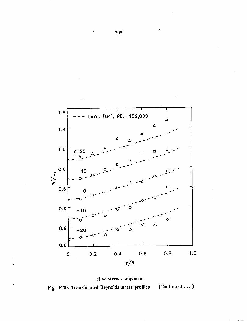
205
I-
1.8
1.4
1.0
0.6
0.6
0.6
0.6
0.6
I l l
LAWN [64], RE=;=109,000
Z_
Z_
¢ --..- n=20 _-" o
10 2-'"jc_-
0
r _ --CT-
m
-101
_ _C r_
0
-2O-0 -_ 0
oc_-"
s
s
s
A
s
s
s
--'o
ss
s-
0
I I I I
0.2 0.4 0.6 0.8
r/R
1.0
c) w' stress component.
Fig. F.IO. Transformed Reynolds stress profiles. (Continued ... )
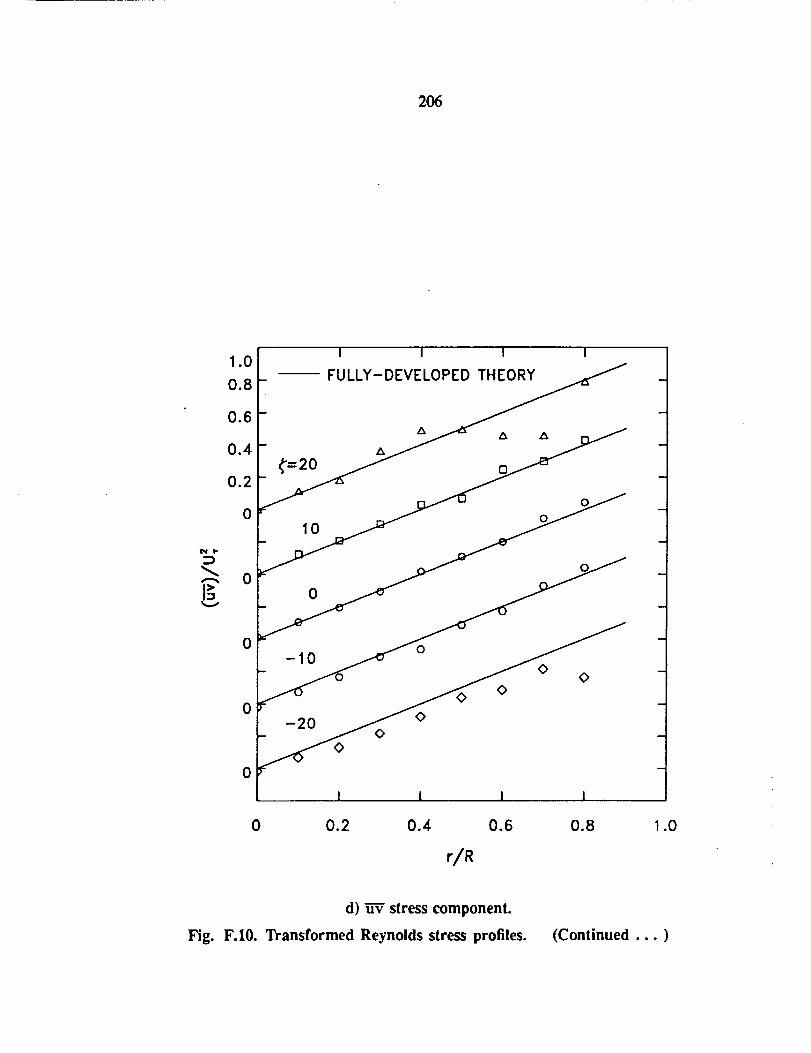
2O6
1.0
0.8
0.6
0.4
0.2
0
}°0
0
0
I I I I
- FULLY- DEVELOPEI_
_ o_ o ___
10 o o
I 1 I I
0 0.2 0.4 0.6 0.8 1.0
r/R
d) _ stress component.
Fig. F.IO. Transformed Reynolds stress profiles. (Continued ... )
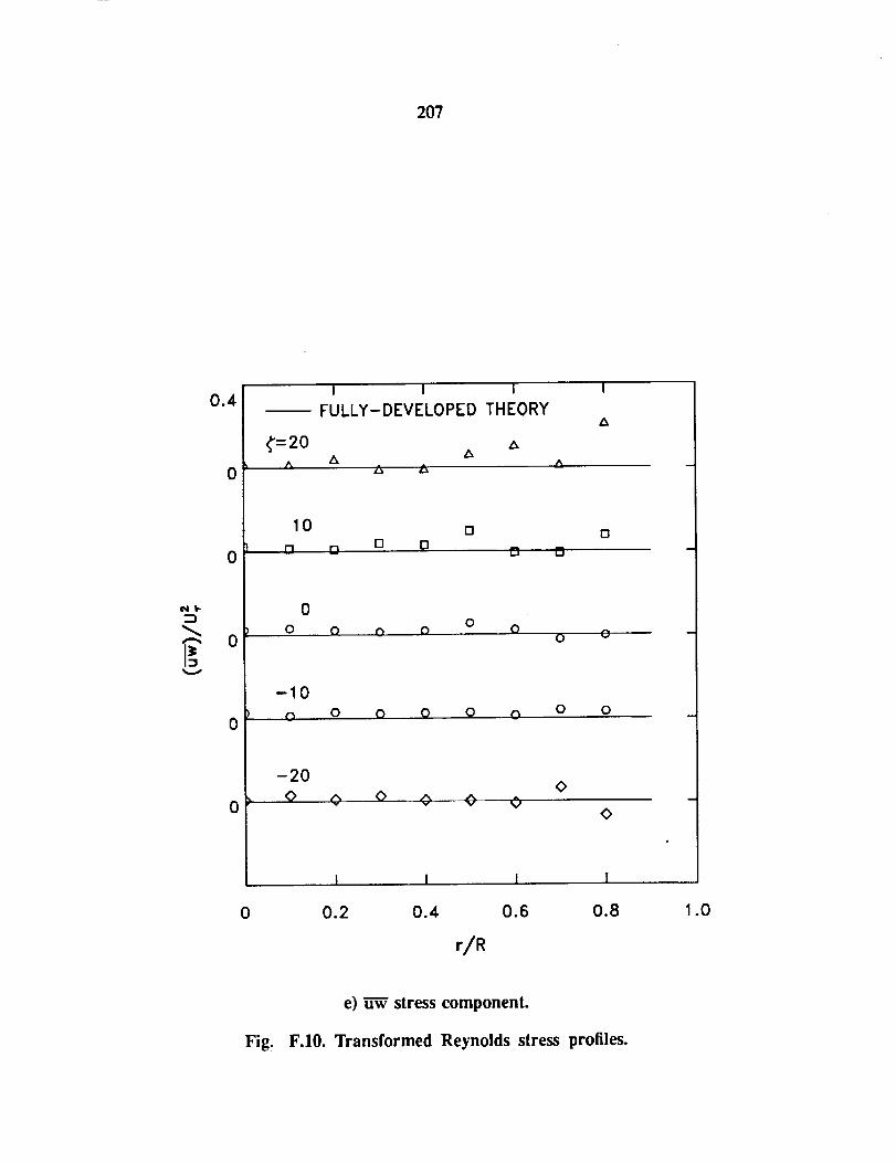
207
V
0.4
0
0
0
0
0
I I I I
FULLY-DEVELOPED THEORYA
C=20 _ A
10 [] o
i _ 0 O 13 m, m,
0
0 0 0 o 0 0 o 0
-I0
0 0 o 0 0 00 0
-20
o O o ¢ ¢ 00
0
I I I I
0 0.2 0.4 0.6 0.8 1.0
r/R
e) _ stress component.
Fig_ F.IO. Transformed Reynolds stress profiles.
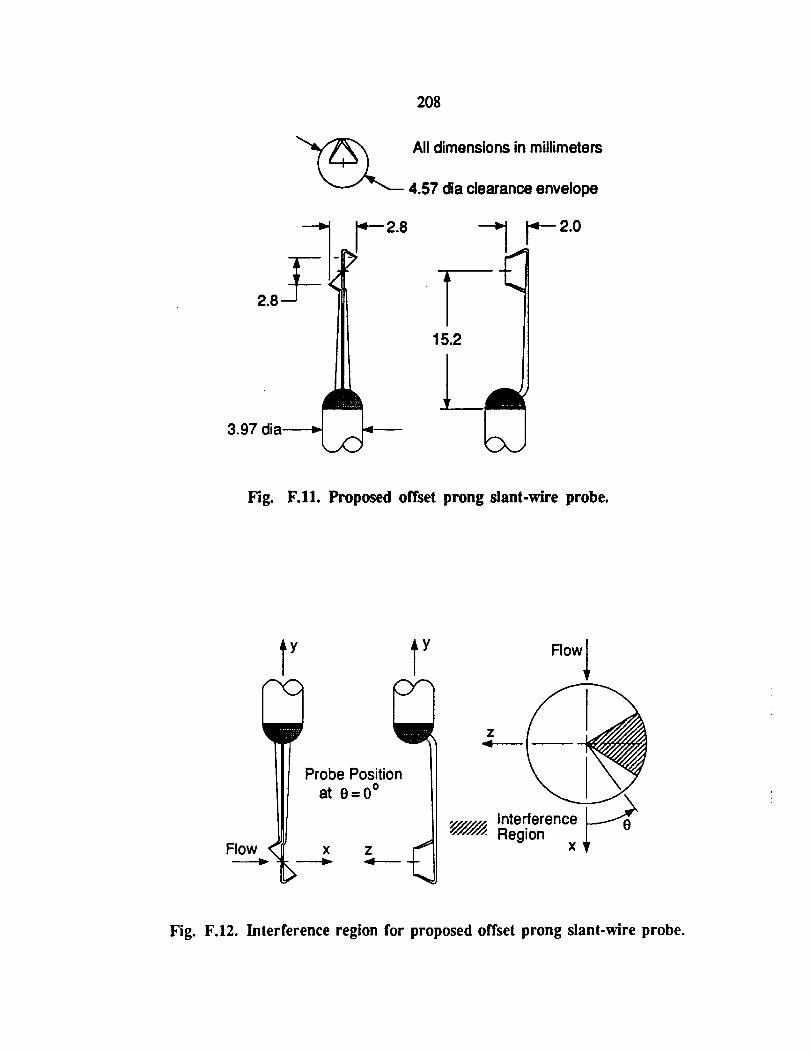
2O8
All dimensions in millimeters
4.57 dia clearance envelope
"_1 F -2"8
28.__1_1-
3.97 ia----_
2.0
Fig. F.11. Proposed offset prong slant-wire probe.
Iy Iy
_Probe Position
] at 0=0°
Flow_
_-- __.
Y7i'77/,__t_irfoerenc; t_
Fig. F.12. Interference region for proposed offset prong slant-wire probe.
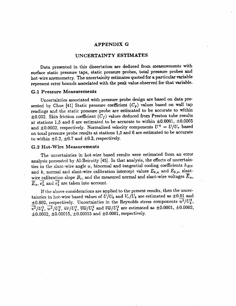
APPENDIX G
UNCERTAINTY ESTIMATES
Data presented in this dissertation are deduced from measurements with
surface static pressure taps, static pressure probes, total pressure probes and
hot-wire anemometry. The uncertainity estimates quoted for a particular variable
represent error bounds associated with the peak value observed for that variable.
G.1 Pressure Measurements
Uncertainties associated with pressure probe design are based on data pre-
sented by Chue [41] Static pressure coefficient (Cp) values based on wall tap
readings and the static pressure probe are estimated to be accurate to within
+0.002. Skin friction coefficient (CI) values deduced from Preston tube results
at stations 1,5 and 6 are estimated to be accurate to within 4-0.0001, 4-0.0005
and 4-0.0002, respectively. Normalized velocity components U + = U/U,. based
on total pressure probe results at stations 1,5 and 6 are estimated to be accurate
to within 4-0.2, 4-0.7 and =t=0.3, respectively.
G.2 Hot-Wire Measurements
The uncertainties in hot-wire based results were estimated from an error
analysis presented by A1-Beirutty [45]. In that analysis, the effects of uncertain-
ties in the slant-wire angle c_, binormal and tangential cooling coefficients hsg
and k, normal and slant-wire calibration intercept values E0,n and E0,s, slant-
wire calibration slope Be, and the measured normal and slant-wire voltages E,,
E,, c_ and es_ are taken into account.
If the above considerations are applied to the present results, then the uncer-
tainties in hot-wire based values of U/Ub and Vr/Ub are estimated as 4-0.01 and
4-0.002, respectively. Uncertainties in the Reynolds stress components -u-ff/U_,
-_'i/U_, w---i/U_, _--5/U:, _"_/U_ and _'-_/U_ are estimated as 4-0.0001, 4-0.0002,
4-0.0002, 4-0.00015, 4-0.00015 and 4-0.0001, respectively.
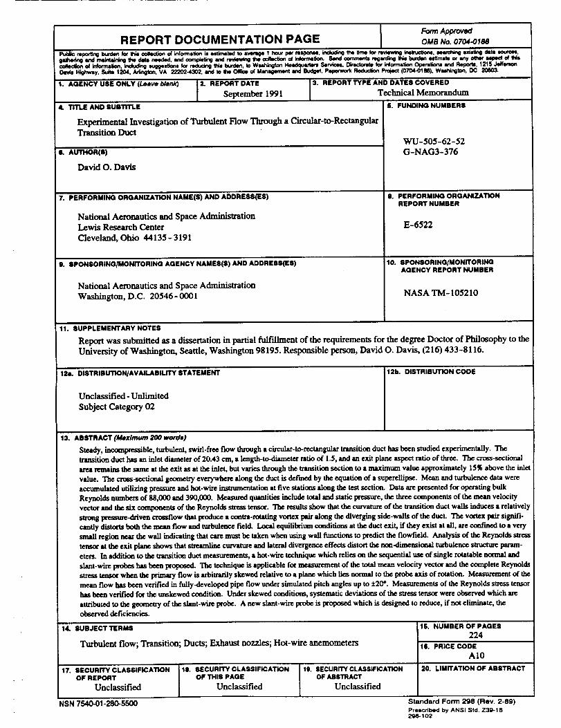
Form ApprovedREPORT DOCUMENTATION PAGE OMBNo.07_.01_
reporS_ burden lot 1*_ _ o_ informa_,n 18 estimated to -vemOe t hour per mspor_, indudlnO the _me for rev',ew_ i_. mw_'r, ir,g exi_l; d1_ m_.m=,
(_.ing =,_d msk_t_i¢_ the ds_ n_d_l, am¢l oomq_eting _r_l _ U_e ¢_t1.¢_,_ oi' Icdocm=6on. S_'_l comments reg=cding _s burd_ _r_m or w_y o_w uped o¢ insoolk0c_cnol _, Indudt_ _=tkm for_ W,=t:_qm, to WJ-,_'_ He_l_u'tor=Servlo_,Btr.ctorm lor _ormaeon Op*r=_ and Report=,1215DavisI.¢_ht_y,_ 1:_4,/_n_on, VA 22202-4.'102,_d to _h_O¢_mo¢M=n=e=_w,_md Bud0_,P=per'_ck_ _ (0704-0_M).Wuhln_ton,OC 2O5O3.
1. AGENCY USE ONLY (Leave bMrdO 2. REPORT DATE 3. REPORT TYPE AND DATES COVERED
September 1991 Technical Memorandum
4. TITLE AND 8UBTITLE
Experimental Investigation of Turbulent Flow Through a Circular-to-RectangularTransition Duct
L AUTHOn(S)
David O. Davis
7. PERFORMING ORGANIZATION NAME(S) AND ADDRE_{ES)
National Aeronautics and Space Administration
Lewis Research Center
Cleveland, Ohio 44135- 3191
S. SPONSORING/MONITORING AGENCY NAMES(S) AND AD[)RESS{ES)
National Aeronautics and Space Administration
Washington, D.C. 20546- 0001
6. FUNDING NUMBERS
WU-505-62-52
G-NAG3-376
0. PERFORMING ORGANIZATIONREPORT NUMBER
E-6522
10. SPON_ORING/MONWORINGAGENCY REPORT NUMBER
NASA TM-105210
11. SUPPLEMENTARY NOTES
Report was submitted as a dissertation in partial fulfflh-nent of the requirements for the degree Doctor of Philosophy to the
University of Washington, Seattle, Washington 98195. Responsible person, David O. Davis, (216) 433-8116.
12a. DiSTRIBUTION/AVAILABILITY STATEMENT
Unclassified - Unlimited
Subject Category 02
12b. DISTRIBUTION CODE
13. ABSTRACT (Maximum 200 wor_)
Stcad_, incompressible, turbulent, swirl-free flow through a circular-to-rectangular transition duct has been studied experimentally. Thetransition duct has an inlet diamet¢: of 20.43 cm, a length-to.diameter ratio of 1.5, and an exit plane aspect ratio of three. The cross-sectionalarea remains the same at the exit as at the inlet, but varies through the transition section to a maximum value approximately 15% above the inlet
value. The cross-sectional geometry everF_bere along the duct is defined by the equation of a superellipse. Mean and turbulence data wereaccumulated utilizing pressure and hot-wire it,.strumentatioa at five stations along the test section. Data ate presented for operating bulk
Reynolds numbers of 88,000 and 390,000. Measured quantities include total and static pressure, the three components of the mean velocityvector and the six components of the Reynolds stress tensor. The results show that the curvature of the transition duct wails induces a relatively
strong pressure-driven croasflow that produce a contra-rotating vortex pair along the diverging side-walis of the duct. The voatex pair signifi-
candy distorts both the mean flow and turbulence field. Local equilibrium conditions at the duct exit, if they exist at all, are co_med to a very
small region near the wall indicating that care must be taken when using wall functions to predict the flowfield` Analysis of the Reynolds stresstensor at the exit plane shows that stzeandine curvature and lateral divergence effects distort the non-ding.nsioo.al turbulence structme param-etevz. In addition to the transition duct measurements, a hot-wire technique which relies on the sequential use of single rotatable normal and
slant-wlre probes has been proposed. The technique is applicable for measurement of the total mean velocity vector and the complete Reynolds
sUess tensor when the primm 7 flow is arbitrarily skewed relative to a plane which lies normal to the probe axis of rotation. Measurement of the
mean flow has been verified in fuliy-developed pipe flow under simulated pitch angles up to *20 =. Measurements of the Reynolds stress tensorhas been verified for the unskewed condition. Under skewed conditions, systematic deviations of the su'ess tensor were observed which are
attributed to the geomeu'y of the slant-wire probe. A new slant-wi_ probe is proposed which is designed to reduce, if not eliminate, theobserved deficiencies.
14. SUBJECT TERMS
Turbulent flow; Transition; Ducts; Exhaust nozzles; Hot-wire anemometers
17. SECURITY CLASSIFICATION 111. SECURITY CLASSIFICATION
OF REPORT OF THIS PAGE
Unclassified Unclassified
ISN 7540-01.280-5500
19. SECURITY CLASSIFICATIONOF ABSTRACT
Unclassified
15. NUMBER OF PAGES224
14. PRICE CODEAI0
20. LIMITATION OF ABSTRACT
Standard Form 298 (Rev. 2-89)Prescribed by ANSI Std. Z39-18298-102