Tufts Data Lab

1

Overlay Analysis II: Using Zonal and Extract Tools to Transfer Raster Values in ArcMap

Created by Patrick Florance and Jonathan Gale, Edited by Carolyn Talmadge on March 2, 2018

If you have raster data that you want to join to existing vector data, you can transfer these data values in ArcMap using

the Spatial Analyst toolbar. For detailed instructions about working with Spatial Analyst in ArcMap 10.5, see the ArcGIS

Desktop Documentation for Extraction tools and Zonal tools.

Skills covered in this Tutorial Include:

Enabling the Spatial Analyst extension

Using the Zonal Statistics Tool to tabulate areas

Using the Extraction Tool to transfer underlying raster data to points

Calculating a percent change using the Field Calculator

Getting Started This exercise uses datasets that are available in the S: drive. For this analysis, we will be joining raster data (Land Cover in

2001 and 2012) with associated districts in Uganda. We will use this process to find the Population per Cropland Area and

Percent Change in Cropland Cover. Follow the steps in the graphics below to perform zonal statistics and extract by point

raster to vector overlay operations.

1. Copy the entire folder S:\Classes\DHP_P207\Uganda_Overlay\ to your H: drive.

2. Check the properties of this copied folder in your H drive and ensure that it is not Read Only. Make sure to check the

Apply this to all subfolders option.

3. From your H Drive, open start.mxd within the Uganda_Overlay folder.

4. In ArcMap, make sure the Spatial Analyst extension is enabled by going to Customize Extensions and check Spatial

Analyst if it is not already checked.

5. Take a moment and review the different layers in the project.

6. All data layers have been projected into UTM Zone 36N. For conducting overlay analysis all data layers must be

projected into the same projected coordinate system.

Using Zonal Statistics to summarize the gridded population of the world data within Uganda Districts 1. Open the ArcToolbox and then navigate to Spatial Analyst Tools Zonal Zonal Statistics as Table. Open the tool

and click the Show Help window to see exactly what this tool does.

Tufts Data Lab

2

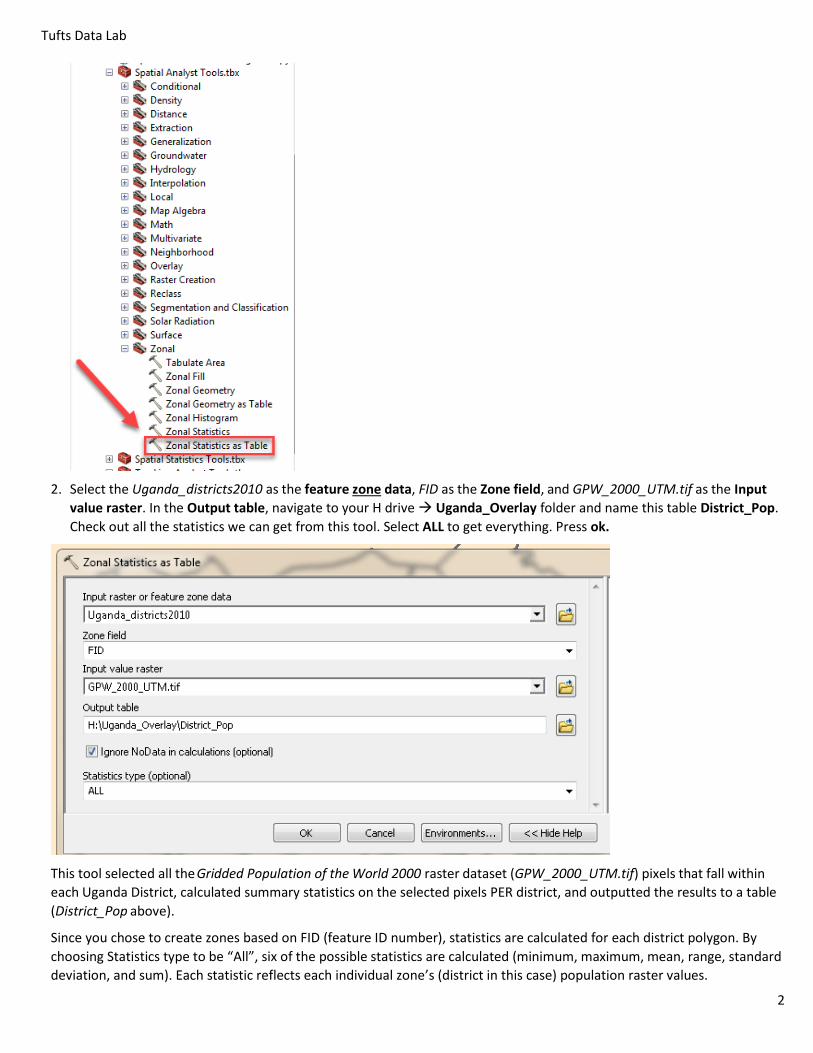
2. Select the Uganda_districts2010 as the feature zone data, FID as the Zone field, and GPW_2000_UTM.tif as the Input

value raster. In the Output table, navigate to your H drive Uganda_Overlay folder and name this table District_Pop.

Check out all the statistics we can get from this tool. Select ALL to get everything. Press ok.

This tool selected all the Gridded Population of the World 2000 raster dataset (GPW_2000_UTM.tif) pixels that fall within

each Uganda District, calculated summary statistics on the selected pixels PER district, and outputted the results to a table

(District_Pop above).

Since you chose to create zones based on FID (feature ID number), statistics are calculated for each district polygon. By

choosing Statistics type to be “All”, six of the possible statistics are calculated (minimum, maximum, mean, range, standard

deviation, and sum). Each statistic reflects each individual zone’s (district in this case) population raster values.

Tufts Data Lab

3

3. Upon completion, the table should appear in the table of contents. The table of contents will switch to List by Source so

that you can see a table has been added. Now, we can join this table to the vector data of districts that we used to

define our zones. Since we chose our zones based on FID, we will be able to join the table to the Uganda_districts2010

layer using that FID field.

4. Right click on the Uganda_districts2010 layer and select Joins and Relates Join.

5. Make sure the tool is set to Join attributes from a table and the new District_pop table is selected in step 2 of the tool.

Then, under Choose the field in this that the join will be based on: Select FID from your districts layer. Likely, ArcMap will

find the matching field for step 3 (also called FID) that the join will be based on. Click Ok. You may be prompted to index

this table. It is ok to do so, though not needed to proceed.

6. Open the attribute table for your Uganda District layer and check that the join was successful.

7. Which field would we use if we wanted to know the total population within a district? Which district has the largest and

smallest population? Right click on the sum field and sort ascending. Now we can see the district with the smallest

population all the way to the district with the largest population.

8. Now, in order to make this join permanent so the statistics remain in the Uganda_Districts2010 attribute table, we

must export the data! Otherwise, the joined statistics data would be dropped the first time we ran a tool. Right click on

the Uganda_Districts2010 layer and select Data Export Data.

Tufts Data Lab

4

9. Click on the folder icon to choose where you want to save your data. Navigate to your H drive and Uganada_Overlay

folder. Name this new shapefile UgandaDistricts_Pop and make sure to save it as a shapefile. Press save and ok.

10. Press Yes when asked if you want to add the exported data to the map as a layer.

11. Open the symbology of this new shapefile and set the graduated colors to SUM so we can visualize the total population

per district.

Use Tabulate Area to summarize 2001 & 2012 Land Cover data into the Uganda Districts 1. If you have a raster dataset that contains categorical data, such as Land Cover, the Zonal Tool Tabulate Area can be

used to transfer and summarize categorical data to a zone such as Uganda Districts.

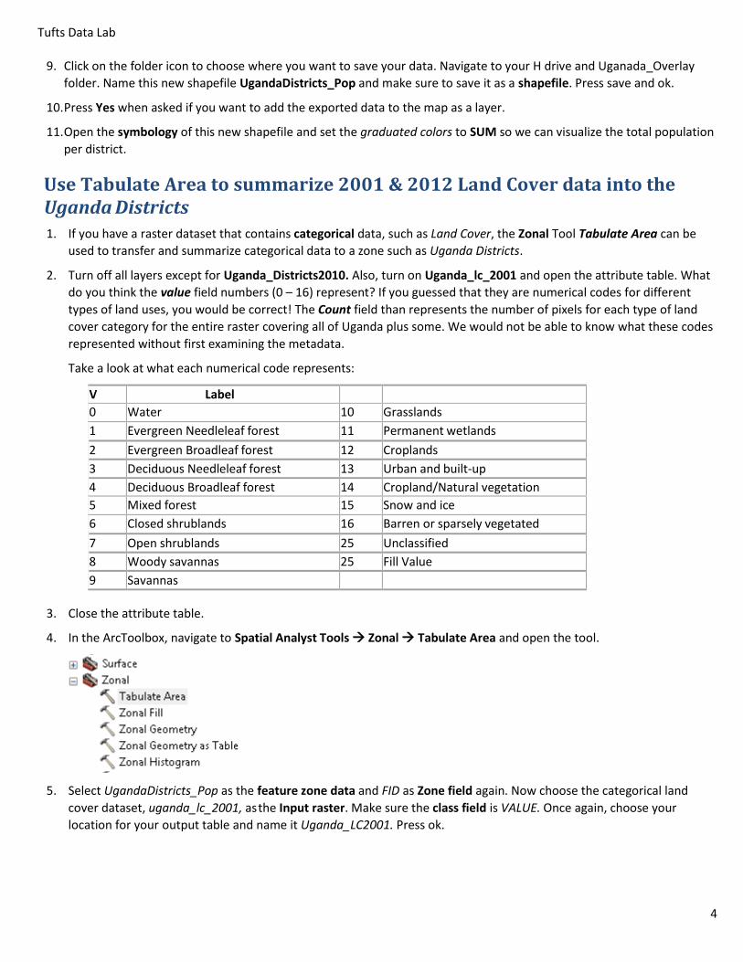
2. Turn off all layers except for Uganda_Districts2010. Also, turn on Uganda_lc_2001 and open the attribute table. What

do you think the value field numbers (0 – 16) represent? If you guessed that they are numerical codes for different

types of land uses, you would be correct! The Count field than represents the number of pixels for each type of land

cover category for the entire raster covering all of Uganda plus some. We would not be able to know what these codes

represented without first examining the metadata.

Take a look at what each numerical code represents:

V

al

u

e

Label

0 Water 10 Grasslands

1 Evergreen Needleleaf forest 11 Permanent wetlands

2 Evergreen Broadleaf forest 12 Croplands

3 Deciduous Needleleaf forest 13 Urban and built-up

4 Deciduous Broadleaf forest 14 Cropland/Natural vegetation

mosaic 5 Mixed forest 15 Snow and ice

6 Closed shrublands 16 Barren or sparsely vegetated

7 Open shrublands 25

4

Unclassified

8 Woody savannas 25

5

Fill Value

9 Savannas

3. Close the attribute table.

4. In the ArcToolbox, navigate to Spatial Analyst Tools Zonal Tabulate Area and open the tool.

5. Select UgandaDistricts_Pop as the feature zone data and FID as Zone field again. Now choose the categorical land

cover dataset, uganda_lc_2001, as the Input raster. Make sure the class field is VALUE. Once again, choose your

location for your output table and name it Uganda_LC2001. Press ok.

Tufts Data Lab

5

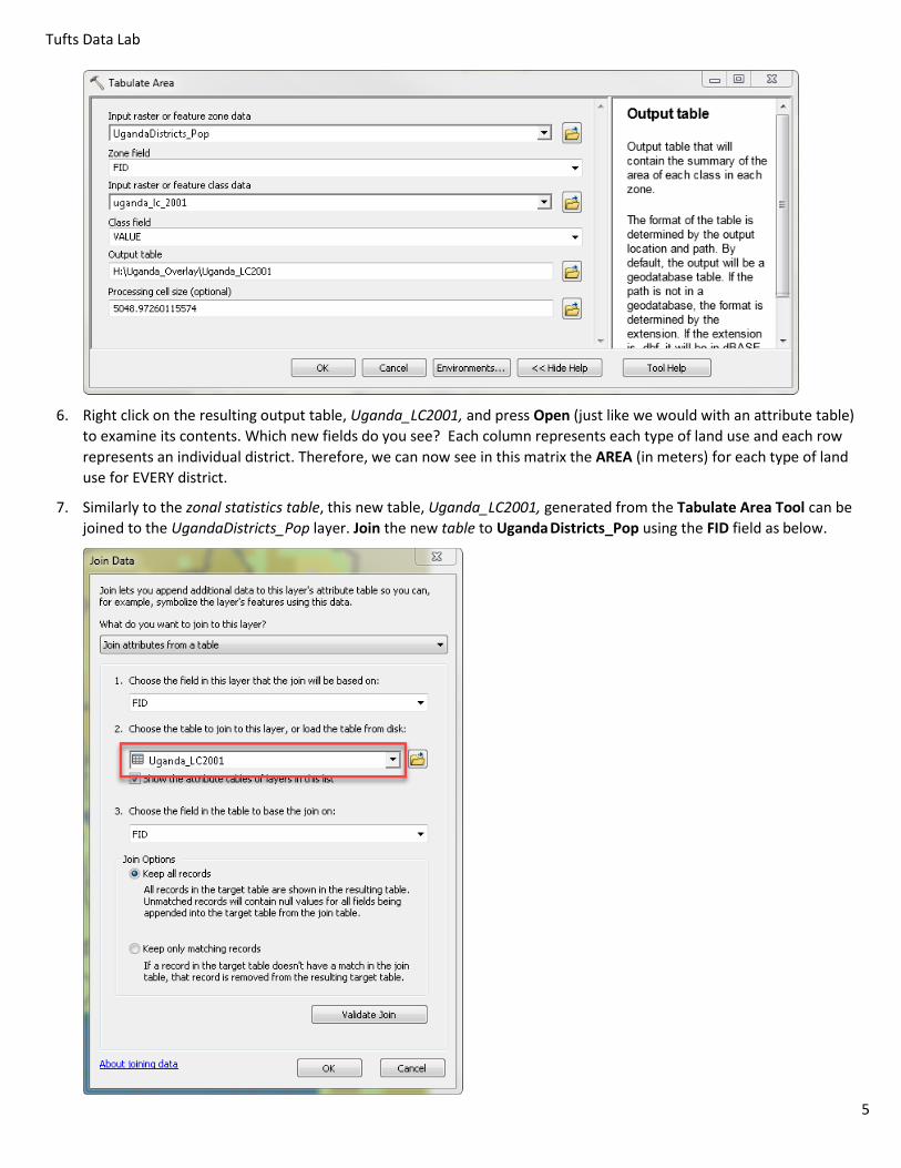
6. Right click on the resulting output table, Uganda_LC2001, and press Open (just like we would with an attribute table)

to examine its contents. Which new fields do you see? Each column represents each type of land use and each row

represents an individual district. Therefore, we can now see in this matrix the AREA (in meters) for each type of land

use for EVERY district.

7. Similarly to the zonal statistics table, this new table, Uganda_LC2001, generated from the Tabulate Area Tool can be

joined to the UgandaDistricts_Pop layer. Join the new table to Uganda Districts_Pop using the FID field as below.

Tufts Data Lab

6

8. Once the Uganda_LC2001 table has been joined to UgandaDistricts_Pop, open the attribute table to make sure it went

smoothly. If all looks good, Export this layer to preserve the join which makes it permanently part of the attribute

table. Name this shapefile UgandaDistricts_Pop_LC2001 and save it in your H drive.

9. Turn on the 2012 land cover dataset, Uganda_lc_2012, and see how it compares to the 2001 land cover dataset.

10. Repeat the Tabulate Area tool calculation with the 2012 land cover data, Uganda_lc_2012. Select

UgandaDistricts_Pop_LC2001 as the feature zone data and Zone field as FID again. Choose the land cover dataset

uganda_lc_2012 as the Input raster. Make sure the class field is VALUE, and once again choose a name

(Uganda_LC2012) and location for your output table.

11. Join this new table to the UgandaDistricts_Pop_LC2001 layer using the FID field as well. Open it up to make sure the

join worked. Check out what all the headings are.

12. Your Uganda Districts should now contain data from the Gridded Population of the World and 2001 and 2012 Land

Cover datasets. Once more, Export the UgandaDistricts_Pop_LC2001 to create a new shapefile that has all 3 of our

joined tables. Call it UgandaDistricts_join.shp and save it in your H drive. Add this new dataset to the map.

13. Save your map session!

Calculating Population per Cropland Area per District You can now perform calculations on the newly calculated data. Below you will calculate the population per each cropland

area for each district.

1. Open the attribute table for this new shapefile, UgandaDistricts_join.

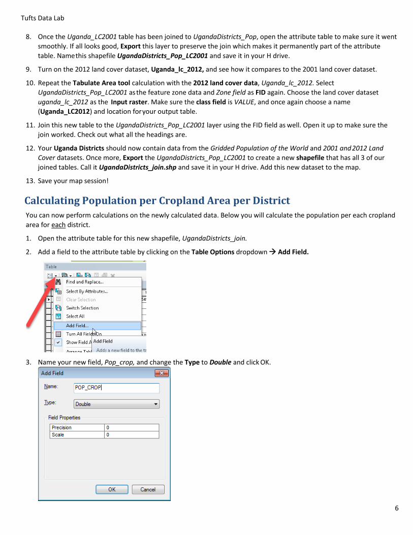
2. Add a field to the attribute table by clicking on the Table Options dropdown Add Field.

3. Name your new field, Pop_crop, and change the Type to Double and click OK.

Tufts Data Lab

7

4. In the attribute table, find this newly created field at the end of the table and right click on the field name Field

Calculator. We will now use the newly created field to estimate the population per cropland area for each zone.

5. In the calculator, double click the field that holds the total population data (aka the SUM field) and divide it by the

column for the 2001 cropland code (value 12) as shown in the table below.

SUM = Summarized Gridded Population of the World

VALUE 12 = 2001 Summarized Cropland Area

6. Symbolize this Population-Cropland Area relationship field using a divergent color model.

Calculating Change in Cropland Land Cover from 2001 to 2012 1. In the same layer, UgandaDistricts_Join, add another field and call it Crop_01_12 and make it a double. This field will

be used to calculate the difference in cropland area from 2001 to 2012 per district.

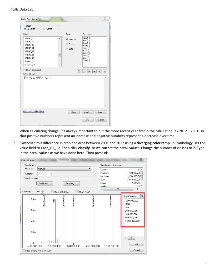
2. Using the Field Calculator, subtract the Value 12 for 2001 from the Value 12 for 2012 (which is actually field

Value_1_13). Why do the field names look different for 2012 in this attribute table compared to how they looked when

we did the join? That is because there cannot be 2 of the same field column headings, so when the join is exported,

ArcMap adds the underscore and second number to help distinguish between the 2001 Value 12 and 2012 Value 12. If

you’re not convinced, look at the attribute table in UgandaDistrricts_Pop_LC2001 which still has the data as a join and

the fields remain in the same order so it’s easy for comparisons.

Tufts Data Lab

8

When calculating change, it’s always important to put the more recent year first in the calculation (ex 2012 – 2001) so

that positive numbers represent an increase and negative numbers represent a decrease over time.

3. Symbolize this difference in cropland area between 2001 and 2012 using a diverging color ramp. In Symbology, set the

value field to Crop_01_12. Then click classify, so we can set the break values. Change the number of classes to 7. Type

in the break values as we have done here. Then press ok.

Tufts Data Lab

9

4. Now we need to make sure the colors accurately represent the numbers. Select the green to red color scheme,

where green will represent an increase in cropland and red will represent a decrease in cropland. Notice how we

need to flip the colors so they represent increase/decreases correctly. Press on Symbol and Flip Symbols.

5. The color for -99 – 100 (representing “no change”) should actually be yellow, not orange (which would imply still a

decrease). Double click on the orange square and set that to a light yellow. Then double click on the 101 – 200000000

color and set that to the lightest green that matches so it starts to represent the increase like so:

6. Adjust the colors individually as you see fit. Press ok and take a look at the map. What message is it sending? Where

are there increases in cropland, decreases, and no change? Check out the example map here.

Tufts Data Lab

10

7. Right click on the layer in the table of contents and press copy. Then go to up the Edit (next to file) and press Paste.

We’ve copied the layer so we can continue to work in this shapefile, but still have a copy with the color scheme we just

worked so hard to create.

8. Now, open the attribute table for UgandaDistricts_join.shp again (the new copy), and add another field titled

PER_CROPS and make it a double. We will calculate the percent change of crop land cover using the Field Calculator.

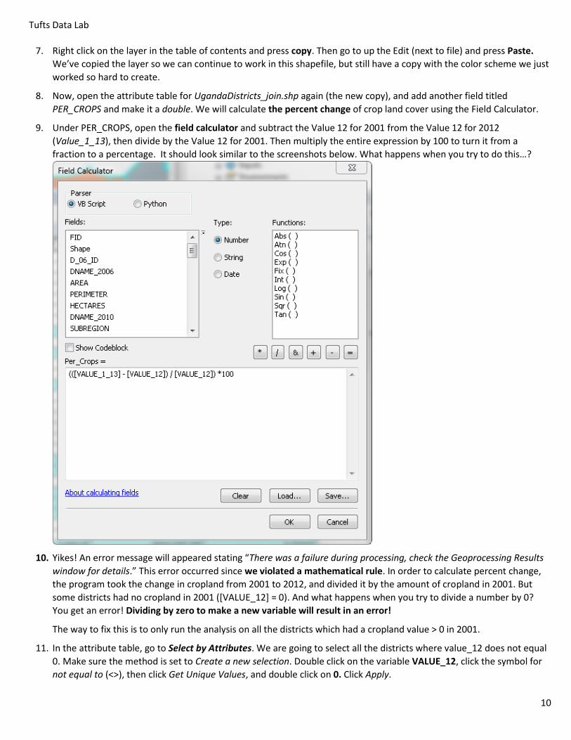
9. Under PER_CROPS, open the field calculator and subtract the Value 12 for 2001 from the Value 12 for 2012

(Value_1_13), then divide by the Value 12 for 2001. Then multiply the entire expression by 100 to turn it from a

fraction to a percentage. It should look similar to the screenshots below. What happens when you try to do this…?

10. Yikes! An error message will appeared stating “There was a failure during processing, check the Geoprocessing Results

window for details.” This error occurred since we violated a mathematical rule. In order to calculate percent change,

the program took the change in cropland from 2001 to 2012, and divided it by the amount of cropland in 2001. But

some districts had no cropland in 2001 ([VALUE_12] = 0). And what happens when you try to divide a number by 0?

You get an error! Dividing by zero to make a new variable will result in an error!

The way to fix this is to only run the analysis on all the districts which had a cropland value > 0 in 2001.

11. In the attribute table, go to Select by Attributes. We are going to select all the districts where value_12 does not equal

0. Make sure the method is set to Create a new selection. Double click on the variable VALUE_12, click the symbol for

not equal to (<>), then click Get Unique Values, and double click on 0. Click Apply.

Tufts Data Lab

11

12. Now that we have all non 0 fields selected, right click on Per_Crops field again and go to Field Calculator. The

expression should still be there, so click OK to run the calculation again. This time it should work because when fields

are selected, tools only run on those selected fields! This is true for all tools in ArcMap (which is why it’s important to

always double check that we do or do not have things selected).

13. Now, you should see the fields which have non-zero values for cropland in 2001 have been calculated correctly and we

did not encounter any error! Which district had the greatest increase in percentage of cropland over the decade?

14. Go ahead and clear your selection. That is good practice to do so since we don’t need those areas selected anymore

and we don’t want it potentially messing up any future calculations.

Extract Underlying Raster Elevation Data to Points Now, we have a layer of villages in Uganda as of January 2009. Perhaps we want to know which of those villages were

located within “cropland” areas in 2012. This might help to understand why there was an increase or decrease in cropland.

1. Turn off all layers except Uganda_Distrcits2010 (which should still be see through). Now, turn on uganda_lc_2012.

Take a second to look it over. Remember what all the different codes mean? Here’s a reminder:

Valu

e

Label

0 Water 10 Grasslands

1 Evergreen Needleleaf forest 11 Permanent wetlands

2 Evergreen Broadleaf forest 12 Croplands

3 Deciduous Needleleaf forest 13 Urban and built-up

4 Deciduous Broadleaf forest 14 Cropland/Natural vegetation

mosaic 5 Mixed forest 15 Snow and ice

6 Closed shrublands 16 Barren or sparsely vegetated

7 Open shrublands 25

4

Unclassified

8 Woody savannas 25

5

Fill Value

9 Savannas

Tufts Data Lab

12

2. Now, turn on Uganda_villages_27Jan09. Is it easy to tell which one of these points fall within cropland? Not for me.

3. Open the attribute table for the villages. Is there any information about which villages fall under what land use

category? Definitely not, but that would be really helpful.

4. We can actually extract information from the underlying land use raster layer and attach it to the points very easily. To

combine raster data with point data, we will use the Extract Values to Points tool to transfer raster values at each point

to the village attribute table. Navigate to Spatial Analyst Tools Extraction Extract Values to Points

5. In the tool, our input point features would be the Uganda villages. And the input raster would be the uganda_lc_2012.

We want to attach the info about the land use to the points. Save it in your H drive Uganda folder and name it

Villages_LandCover.

6. Now, we have a new point file of the villages. Open the attribute table. A new field has been added to the points that

has the raster value from the land cover raster dataset. Here we can see that the code for each land use that the village

falls within has now been added.

Unlike zonal statistics as table, this land cover data has already been added and we don’t have to go through the steps

of joining it to the attribute table!

Tufts Data Lab

13

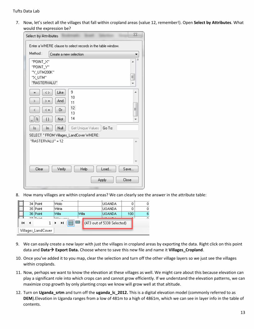
7. Now, let’s select all the villages that fall within cropland areas (value 12, remember!). Open Select by Attributes. What

would the expression be?

8. How many villages are within cropland areas? We can clearly see the answer in the attribute table:

9. We can easily create a new layer with just the villages in cropland areas by exporting the data. Right click on this point

data and Data Export Data. Choose where to save this new file and name it Villages_Cropland.

10. Once you’ve added it to you map, clear the selection and turn off the other village layers so we just see the villages

within croplands.

11. Now, perhaps we want to know the elevation at these villages as well. We might care about this because elevation can

play a significant role into which crops can and cannot grow efficiently. If we understand the elevation patterns, we can

maximize crop growth by only planting crops we know will grow well at that altitude.

12. Turn on Uganda_srtm and turn off the uganda_lc_2012. This is a digital elevation model (commonly referred to as

DEM).Elevation in Uganda ranges from a low of 481m to a high of 4861m, which we can see in layer info in the table of

contents.

Tufts Data Lab

14

13. Sometimes the black to white color scheme makes it harder to visualize the elevation so let’s change it. Open the

symbology for the elevation layer. Notice how symbology for rasters looks a bit different than the symbology options

for vectors. Stay in the stretched option and pick a different color ramp – perhaps a divulging color ramp so it’s easier

to see the extreme highs and lows. Press ok. Now we can start to get a much better idea of really high and low lying

lands.

14. Open the attribute table for Uganda_Srtm. What does the value column represent? Those are the individual elevations

in meters. How do I know they are meters? Because our projection uses meters and therefore so does the data! Wat

does the Count field represent? Those are the number of cells that have that specific elevation.

15. Do our villages_cropland layer have any info about elevation in the attribute table. No, definitely not. But using the

same tool, Extract Values to Points, we can easily calculate that info!

16. Navigate to Spatial Analyst Tools Extraction Extract Values to Points

17. Now the input point features are the new Villages_Cropland and the input raster is the uganda_srtm. Once again, save

in your H drive and name it Villages_Cropland_Elevation.

18. When we try to run the tool, we get another error. That’s frustrating and the error code is not very helpful. The reason

we are getting an error is because it’s trying to create a new field in the point layer called “RasterValu” to hold the

elevation values. The problem is there is already a field in this village_cropland point layer called “rastervalu” that

holds the info from the land cover dataset – so the tool fails because the field name is not unique.

19. However, since we purposefully selected all the points that fall within cropland land cover (12), we don’t really need

this field. Open the Villages_Cropland attribute table. The RasterValue column should ONLY have 12’s in it because

that is what we selected for. Therefore, we don’t really need this field since we know these are villages in cropland

already. Right click on RasterValu and Delete Field.

20. Now, try rerunning the Extract Values to Points tool using the same inputs. The tools should run no problem now

because it is able to create the new RasterValu field that will hold the elevation values.

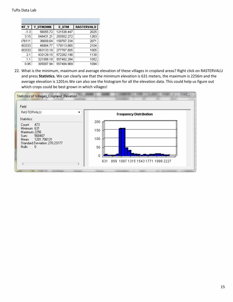
21. Open the attribute table for this new point village’s layer. Now there is another RATERVALU field that shows the

elevation of these villages that are only within cropland!

Tufts Data Lab

15

22. What is the minimum, maximum and average elevation of these villages in cropland areas? Right click on RASTERVALU

and press Statistics. We can clearly see that the minimum elevation is 631 meters, the maximum is 2256m and the

average elevation is 1201m.We can also see the histogram for all the elevation data. This could help us figure out

which crops could be best grown in which villages!