APPENDIX J Tsunami Report

TSUNAMI HAZARD ASSESSMENT FOR THE PORTS OF LONG BEACH AND LOS ANGELES

FINAL REPORT

Prepared for:

PORT OF LONG BEACH 925 Harbor Plaza

Long Beach, California 90801

PORT OF LOS ANGELES 425 S. Palos Verdes Street

San Pedro, California 90733

Prepared by:

MOFFATT & NICHOL 3780 Kilroy Airport Way, Suite 600

Long Beach, California 90806

April 2007

M&N File: 4839-169

-i-

PREFACE This report is the result of a project jointly funded by the Port of Los Angeles and the Port of Long Beach and conducted by Moffatt & Nichol. In addition to guidance from the Ports, Dr. Frederic Raichlen, Professor Emeritus, California Institute of Technology participated in the project as a technical advisor and report reviewer as well as preparing the section in this report regarding distant tsunami sources and resultant tsunamis in the Ports. Mr. Bruce Schell of Earth Mechanics, Inc. prepared the section on potential local tsunami sources which includes an assessment of the probability of the various sources. Dr. Jose Borrero from the University of Southern California assisted in the report review and also provided the initial tsunami characteristics from the various potential sources to be used as the boundary conditions to the detailed tsunami propagation modeling. Additional review of the entire report was provided by Dr. Costas Synolakis from the University of Southern California. This final report incorporates comments from the Ports and participating reviewers.

-ii-

CONTENTS 1.0 INTRODUCTION ............................................................................................... 1

1.1 Background.......................................................................................................... 1

1.2 Scope of Work ..................................................................................................... 1 2.0 TSUNAMI SOURCES ........................................................................................ 3

2.1 Distant Tsunami sources...................................................................................... 3

2.2 Potential Local Tsunami Sources ...................................................................... 15

2.2.1 Geologic Setting ................................................................................................ 16

2.2.2 Seismological Setting ........................................................................................ 18

2.2.3 Tectonic Setting ................................................................................................. 21

2.2.4 Tsunami Origins and Dynamics ........................................................................ 23

2.2.5 Earthquake and Tsunami Recurrence ................................................................ 25

2.2.6 Submerged Landslides....................................................................................... 27 3.0 HYDRODYNAMIC MODEL DEVELOPMENT ............................................ 30

3.1 MIKE 21 - BW Model Description ................................................................... 30

3.2 Benchmark Test ................................................................................................. 30

3.3 Model Setup For POLA/POLB ......................................................................... 34

3.4 Initial Tsunami Generation at the Sources......................................................... 38

3.5 Hydrodynamic Model Still Water Level ........................................................... 41 4.0 MODEL SIMULATION RESULTS ................................................................. 43

4.1 Maximum Water Levels .................................................................................... 43

4.1.1 Maximum Water Levels in POLA..................................................................... 51

4.1.2 Maximum Water Levels in POLB..................................................................... 52

4.2 Water Level Time Histories............................................................................... 53

4.3 Tsunami Travel Times ....................................................................................... 68

4.4 Current Speeds in the Channels ......................................................................... 68

4.4.1 Current Speeds in POLA ................................................................................... 69

4.4.2 Current Speeds in POLB.................................................................................... 73

4.5 Overtopping Assessment ................................................................................... 77 5.0 MODEL SENSITIVITY SIMULATIONS........................................................ 78

5.1 Federal Breakwater Sensitivity.......................................................................... 78

5.2 Impacts of Scaling Wave Amplitudes ............................................................... 79 6.0 CONCLUSIONS................................................................................................ 84 7.0 REFERENCES .................................................................................................. 86

-iii-

List of Figures Figure 2-1 Tide Gage Records at POLA Berth 60 for the 1960 Chilean Tsunami and the

1964 Alaskan Tsunami ........................................................................................ 4 Figure 2-2 Up-crossing Wave Height as a Function of Time for the 1960 Chilean Tsunami at

POLA, Berth 60 ................................................................................................... 4 Figure 2-3 Normalized Energy Spectra for the 1960 Chilean Tsunami and the 1964 Alaskan

Tsunami in POLA, Berth 60, and in Ensenada, Mexico...................................... 5 Figure 2-4 Normalized Energy Spectra for the 1964 Alaskan Tsunami at POLA Berth 60,

Santa Monica, and La Jolla.................................................................................. 6 Figure 2-5 Bathymetry of the Southern California Bight from Point Conception to the

Mexican border .................................................................................................... 7 Figure 2-6 Frequency Distribution of Wave Heights in POLA and POLB for the 1922

Chilean Tsunami, the 1946 Aleutian Tsunami, the 1960 Chilean Tsunami and the 1964 Alaskan Tsunami .................................................................................. 8

Figure 2-7 Frequency Distribution of Normalized Wave Heights in POLA and POLB for the 1922 Chilean Tsunami, the 1946 Aleutian Tsunami, the 1960 Chilean Tsunami and the 1964 Alaskan Tsunami Compared to a Rayleigh Distribution ............... 9

Figure 2-8 The Variation of the Mean Wave Height with Seismic Moment for Two Alaskan and Two Chilean Events .................................................................................... 10

Figure 2-9 A Comparison of the Wave Heights in POLA and POLB for the May 23, 1960 Chilean Tsunami to a Rayleigh Distribution ..................................................... 11

Figure 2-10 Water Surface Time History in the Port of Los Angeles of the 1952 Kamchatka Tsunami ............................................................................................................. 13

Figure 2-11 Water Surface Time History in the Port of Los Angeles of the 11/15/06 Kuril Islands Tsunami ................................................................................................. 13

Figure 2-12 Wave Height Distributions in the Port of Los Angeles for the 1952 Kamchatka Tsunami ............................................................................................................. 14

Figure 2-13 Tsunamigenic Sources from Borrero et al. (2004).............................................. 16 Figure 2-14 Generalized and Simplified Traces of Major Faults and Provinces within and

Surrounding the Southern California Continental Borderland. ......................... 17 Figure 2-15 Map Showing Major Faults and Recent Seismicity (M ≥ 4) of the Southern

California Region. Some of the More Notable Events are Shown by Stars. From Legg et al., 2004....................................................................................... 19

Figure 2-16 Sketch Map Showing Slip Rates on Major Faults in Southern California. The numbers are slip rates in millimeters per year. .................................................. 22

Figure 2-17 Earthquake Recurrence Interval based on Earthquake Magnitude .................... 27 Figure 3-1 Bathymetry of Benchmark Test ........................................................................... 31 Figure 3-2 Boundary Input Water Levels Benchmark Test................................................... 31 Figure 3-3 Benchmark Test Output Gage Locations ............................................................. 32 Figure 3-4 Water Level Comparison at Gage 1 ..................................................................... 32 Figure 3-5 Water Level Comparison at Gage 2 ..................................................................... 33 Figure 3-6 Water Level Comparison at Gage 3 ..................................................................... 33 Figure 3-7 MIKE21-BW Model Bathymetry ........................................................................ 34 Figure 3-8 Boundary Input for the Catalina Fault - 7 Segments Scenario............................. 35 Figure 3-9 Boundary Input for the Catalina Fault - 4 Segments Scenario............................. 35

-iv-

Figure 3-10 Boundary Input for the Lasuen Knoll Fault Scenario ........................................ 36 Figure 3-11 Boundary Input for the San Mateo Thrust Fault Scenario ................................. 36 Figure 3-12 Boundary Input for the Palos Verdes Landslide I Scenario............................... 37 Figure 3-13 Boundary Input for the Palos Verdes Landslide II Scenario.............................. 37 Figure 3-14 Boundary Input for Cascadia Mw=9.2 Scenario................................................. 38 Figure 3-15 Location of the Local Palos Verdes Landslide Tsunami Sources...................... 40 Figure 3-16 Cumulative Frequency Distribution of Water Levels in POLA/POLB over a 19-

year Tidal Epoch................................................................................................ 42 Figure 4-1 Maximum Water Levels for the Catalina Fault - 7 Segments Scenario............... 44 Figure 4-2 Maximum Water Levels for the Catalina Fault - 4 Segments Scenario............... 45 Figure 4-3 Maximum Water Levels for the Lasuen Knoll Fault Scenario ............................ 46 Figure 4-4 Maximum Water Levels for the San Mateo Thrust Fault .................................... 47 Figure 4-5 Maximum Water Levels for the Palos Verdes Landslide I Scenario ................... 48 Figure 4-6 Maximum Water Levels for the Palos Verdes Landslide II Scenario.................. 49 Figure 4-7 Maximum Water Levels for the Cascadia Mw=9.2 Scenario............................... 50 Figure 4-8 Water Level Gage Locations................................................................................ 51 Figure 4-9 Water Levels in POLA for the Catalina Fault - 7 Segments Scenario................. 54 Figure 4-10 Water Levels in POLA for the Catalina Fault – 4 Segments Scenario .............. 55 Figure 4-11 Water Levels in POLA for the Lasuen Knoll Fault Scenario ............................ 56 Figure 4-12 Water Levels in POLA for the Santa Mateo Thrust Fault Scenario .................. 57 Figure 4-13 Water Levels in POLA for the Palos Verdes Landslide I Scenario ................... 58 Figure 4-14 Water Levels in POLA for the Palos Verdes Landslide II Scenario.................. 59 Figure 4-15 Water Levels in POLA for Cascadia Mw=9.2 Scenario..................................... 60 Figure 4-16 Water Levels in POLB for the Catalina Fault - 7 Segments Scenario ............... 61 Figure 4-17 Water Levels in POLB for the Catalina Fault - 4 Segments Scenario ............... 62 Figure 4-18 Water Levels in POLB for the Lasuen Knoll Fault Scenario............................. 63 Figure 4-19 Water Levels in POLB for the Santa Mateo Thrust Fault Scenario................... 64 Figure 4-20 Water Levels in POLB for the Palos Verdes I Scenario .................................... 65 Figure 4-21 Water Levels in POLB for the Palos Verdes II Scenario................................... 66 Figure 4-22 Water Levels in POLB for the Cascadia Mw=9.2 Scenario ............................... 67 Figure 4-23 Current Speed Gage Locations........................................................................... 69 Figure 4-24 Currents in POLA for the Catalina Fault - 7 Segments Scenario ...................... 70 Figure 4-25 Currents in POLA for the Catalina Fault - 4 Segments Scenario ...................... 70 Figure 4-26 Currents in POLA for the Lasuen Knoll Fault ................................................... 71 Figure 4-27 Currents in POLA for the San Mateo Thrust Fault ............................................ 71 Figure 4-28 Currents in POLA for the Palos Verdes I Scenario............................................ 72 Figure 4-29 Currents in POLA for the Palos Verdes II Scenario .......................................... 72 Figure 4-30 Currents in POLA for the Cascadia Mw=9.2 Scenario....................................... 73 Figure 4-31 Currents in POLB for the Catalina Fault - 7 Segments Scenario....................... 74 Figure 4-32 Currents in POLB for the Catalina Fault - 4 Segments Scenario....................... 74 Figure 4-33 Currents in POLB for the Lasuen Knoll Fault ................................................... 75 Figure 4-34 Currents in POLB for the San Mateo Thrust Fault ............................................ 75 Figure 4-35 Currents in POLB for the Palos Verdes I Scenario............................................ 76 Figure 4-36 Currents in POLB for the Palos Verdes II Scenario .......................................... 76 Figure 4-37 Currents in POLB for the Cascadia Mw=9.2 Scenario...................................... 77

-v-

Figure 5-1 Comparison of Water Levels in POLA between With and Without Federal Breakwaters for the Palos Verdes I Scenario..................................................... 78

Figure 5-2 Comparison of Water Levels in POLB between With and Without Federal Breakwaters for the Palos Verdes I Scenario..................................................... 79

Figure 5-3 Comparison of Water Levels between Scaled and Prototype Wave Amplitude Inputs in POLA.................................................................................................. 80

Figure 5-4 Comparison of Water Levels between Scaled and Prototype Wave Amplitude Inputs in POLB .................................................................................................. 81

Figure 5-5 Comparison of Fluxes between Scaled and Prototype Wave Amplitude Inputs in POLA................................................................................................................. 81

Figure 5-6 Comparison of Fluxes between Scaled and Prototype Wave Amplitude Inputs in POLB ................................................................................................................. 82

Figure 5-7 Comparison of Flux Directions between Scaled and Prototype Wave Amplitude Inputs in POLA.................................................................................................. 82

Figure 5-8 Comparison of Flux Directions between Scaled and Prototype Wave Amplitude Inputs in POLB .................................................................................................. 83

List of Tables Table 2-1 Earthquakes and Corresponding Seismic Moments ……………………………..10

Table 2-2 Notable Historical Earthquakes in Southern California Offshore Region……….20

Table 3-1 Benchmark Test Condition Summary……………………………………….…...30

Table 3-2 Earthquake Source Parameters for Tsunami Simulations ……………………….39

Table 3-3 Range of Maximum Coseismic Uplift Values for Each Initial Condition……….39

Table 4-1 Maximum Water Levels in Port of Los Angeles (Meters, MSL)………………..52

Table 4-2 Maximum Water Levels in Port of Long Beach (Meters, MSL)………………...52

Table 4-3 Tsunami Arrival Times and Characteristic Wave Periods……………………….68

-1-

1.0 INTRODUCTION

1.1 BACKGROUND There is currently renewed interest in the potential for tsunamis along the southern California coast and the associated impacts to the Ports of Los Angeles and Long Beach (POLA/POLB), particularly in light of the devastation caused by the recent Indian Ocean earthquake and tsunami of December 26, 2004. Historically, concern for tsunamis along the California coast has been limited to distant sources such as Alaska, Chile, or others. A detailed assessment of distant tsunami source impacts conducted by Houston (1980) has been used for design guidelines to the present time. However, a few studies have been published recently suggesting potential tsunami sources within the southern California Bight which could have a greater impact to POLA/POLB due to the short travel distance and higher amplitudes than expected from the remote sources (Legg et al., 2004 and Borrero et al., 2004).

The Ports have authorized Moffatt & Nichol to conduct a study of potential local tsunamigenic sources and potential impacts to the Ports. This investigation is to include more detailed analysis of the tsunami propagation into the Ports than is available from other recent studies. The study expands on the previous work in that it includes more details regarding local maximum water levels, current speeds, arrival times, and overtopping rates at selected locations. The results described in this report are limited to the hydrodynamic modeling of the tsunami propagation to provide information for further evaluation of impacts to the Port infrastructure. A second phase of the work would include evaluation of the hydrodynamic impacts such as moored and moving vessel issues, structural impacts associated with flooding of Port facilities, and personnel safety issues.

While the model used for the detailed tsunami propagation into POLA/POLB included areas outside of the Ports, the results of the analysis are limited to POLA/POLB since no attempt was made to represent the adjacent areas rigorously other than as necessary to limit boundary condition impacts to the model results in the Ports. It should also be recognized the tsunami scenarios evaluated in this report are representative of a range of local sources that have been identified as possible but does not necessarily represent all potential local sources. The range of local sources is useful for identifying the more severe tsunami propagation directions and characteristics. The likelihood of the occurrence of these potential sources is also discussed to place the results in the proper perspective for the design of coastal structures.

1.2 SCOPE OF WORK The scope of work for this study includes the following:

1) Conduct a review of historical tsunamis impacting POLA/POLB.

2) Identify and evaluate the likelihood of potential local tsunamigenic sources.

3) Generate the initial tsunami wave from each potential source.

4) Configure an applicable detailed hydrodynamic model for POLA/POLB.

-2-

5) Propagate the identified potential tsunami waves into POLA/POLB with a detailed hydrodynamic model of the area.

6) Describe the tsunami characteristics in the Ports including predicted water levels, current speeds, and arrival times.

7) Determine overtopping characteristics at locations where maximum water levels exceed adjacent land elevations.

The review of historical tsunamis in POLA/POLB is discussed in Section 2 along with the identification of the potential local sources. Section 3 describes the development of the hydrodynamic model, the configuration of the model for POLA/POLB, and the initial tsunami wave generation and application along the hydrodynamic model boundary. The results of the model simulations are discussed in Section 4 and a sensitivity analysis is discussed in Section 5. Section 6 presents the conclusions of this study.

-3-

2.0 TSUNAMI SOURCES

2.1 DISTANT TSUNAMI SOURCES Over the years POLA/POLB have been exposed to distant tsunamis from sources located in Alaska and Chile. These events included the 1922 Chilean tsunami (Mw = 8.4), the 1946 Aleutian tsunami (Mw = 7.8), the 1960 Chilean tsunami (Mw = 9.5), and the 1964 Alaskan tsunami (Mw = 9.2); these will be discussed herein. The basic data for this analysis were obtained from Wilson (1971), Raichlen (1972), Berkman and Symons (1964), and Spaeth and Berkman (1967).

An example of the tide gage records (marigrams) used is presented in Figure 2-1. These were obtained at Berth 60 in POLA for the tsunamis of May 23-24, 1960 (Chilean) and March 28-29, 1964 (Alaskan). The duration of these two records was 22 hrs and 24 hrs, respectively. In both cases the initial wave was positive with the oscillations apparently relatively undiminished for the period shown. The round-trip tsunami travel time from the west coast of the U.S. to Japan is approximately 30 hrs. Thus, the records presented in Figure 2-1 are apparently water level changes that occurred before the reflected waves from the western Pacific Rim have returned to the West Coast.

In Figure 2-2 the wave heights obtained from the continuous tide gage record of Figure 2-1 for the 1960 Chilean event are presented. These wave heights are taken directly from the tide gage record using the up-crossing method, i.e., the height of the wave from the trough to the following crest. In this way the astronomical tide is essentially eliminated from the data. A surprising feature of this figure is the apparent minimal damping that takes place over the 20 hour duration of the record. (This has been found to be the case at several other locations around the Pacific Ocean.) This suggests the response function to waves in the area of the tide gage is very sharply peaked; not like the smoothly varying response curves seen for a highly damped dynamic system.

Normalized energy spectra are presented in Figure 2-3 for POLA Berth 60 and for Ensenada, Mexico for the 1960 Chilean tsunami and the 1964 Alaskan event. These spectra are obtained by a spectral process that has a relatively low resolution and emphasizes the major lower frequencies. What is striking in Figure 2-3 is the spectra at each location for the two different events are nearly identical. Shown in the figures are the root mean square of the measured water surface time histories. This is a measure of the intensity of the local tsunami induced oscillations. It is seen at POLA the 1960 event resulted in waves with a root mean square about 72% greater for the Chilean tsunami compared to the Alaskan tsunami. At Ensenada the tsunami from the Chilean event was about 35% greater than that generated by the Alaskan earthquake. These differences are reasonable for at least two reasons: (1) The magnitude of the Chilean earthquake was 9.5 compared to about 9.2 for the Alaskan earthquake (the 2004 Sumatra earthquake had a magnitude of about 9.3) and (2) It may be the propagation route relative to the orientation of the coast at these two locations was more favorable for the Chilean tsunami than for the Alaskan tsunami. Since these are two different tectonic events it is apparent that either the local embayments where the waves are measured are being set into resonance by the tsunamis or the whole offshore waters are being excited and this wave induced activity offshore is driving the harbors.

-4-

Figure 2-1 Tide Gage Records at POLA Berth 60 for the 1960 Chilean Tsunami and

the 1964 Alaskan Tsunami

0.0

1.0

2.0

3.0

4.0

5.0

6.0

H (

ft)

0.0 1.0 2.0 3.0 4.0 5.0 6.0 7.0 8.0 9.0 10.0 11.0 12.0 13.0 14.0 15.0 16.0 17.0 18.0 19.0 20.0

T (hr)

LA Berth 60 1960

H (ft)

Figure 2-2 Up-crossing Wave Height as a Function of Time for the 1960 Chilean

Tsunami at POLA, Berth 60

-5-

Figure 2-3 Normalized Energy Spectra for the 1960 Chilean Tsunami and the 1964

Alaskan Tsunami in POLA, Berth 60, and in Ensenada, Mexico

To investigate the influence of the offshore waters on the wave amplitudes in POLA/POLB, normalized spectra were obtained at three locations along the southern California coast within the Southern California Bight: Santa Monica, POLA Berth 60, and La Jolla for the Alaskan tsunami of 1964. These are presented in Figure 2-4. Although there is some variation of the spectra and hence the wave heights at the three locations (the latter shown by

-6-

variation of the root mean square of the wave heights) there is a striking similarity to the spectra. At each location there are two major peaks in the spectra at a frequency of about 0.5 hr-1 and at 1.6 hr-1 or periods of 2 hrs and 0.63 hrs (37.5 min), respectively. Since these locations are of the order of 150 mi apart, this suggests the offshore waters are put into oscillation by the incident tsunamis. The recorded water surface fluctuations in POLA and POLB are probably caused by the movement of offshore waters and not the tsunami itself. In other words it might be the initial waves of the tsunami that excite the offshore waters into relatively long duration oscillations.

Figure 2-4 Normalized Energy Spectra for the 1964 Alaskan Tsunami at POLA Berth

60, Santa Monica, and La Jolla A bathymetric chart of the region from about Pt. Conception southward to the Mexican border is presented in Figure 2-5. The chart shows several important features. The first apparent feature at each of these three locations is the large nearshore shelves, e.g., the San Pedro shelf and the shelf in Santa Monica Bay. In addition, for the region essentially from Santa Barbara southward past San Pedro Bay there are a series of offshore basins which are limited in the seaward direction (westward) by the chain of offshore islands. It has been suggested this complex region is placed into oscillation by incident tsunamis such that what is recorded at the coastal tide gage stations is not the tsunami itself but the result of the interaction of the tsunami with the bays and basins.

Water surface time histories of the four events taken from Wilson (1971), Berkman and Symons (1964), and Spaeth and Berkman (1967) were used to define the range of wave heights in the POLA/POLB harbors resulting in wave height data such as presented in Figure 2-2. These data were then ordered in decreasing height and frequency distributions were obtained. The results are presented in Figure 2-6 where the wave height (the distance from the trough to following crest), the ordinate, is shown as a function of the percent of waves in the record with wave heights greater than the indicated wave height. For example, at Pier 2

-7-

of POLB for the 1960 Chilean tsunami, 50 % of the waves had heights greater than about 0.8 m (2.6 ft). The maximum waves measured were for the 1960 Chilean tsunami in both POLA and POLB and were about 1.40 m to 1.7 m (4.6 ft to 5.5 ft) at three locations in POLA and POLB. (It should be noted that the configuration of the harbor has changed over the years compared with what exists today in both POLA and POLB, and this will be discussed later.)

Figure 2-5 Bathymetry of the Southern California Bight from Point Conception to the

Mexican border

-8-

Figure 2-6 Frequency Distribution of Wave Heights in POLA and POLB for the 1922 Chilean Tsunami, the 1946 Aleutian Tsunami, the 1960 Chilean Tsunami and the 1964

Alaskan Tsunami In Figure 2-7, the wave height data for each location and each event shown in Figure 2-6 have been divided by the mean wave height and are presented as a function of the frequency of occurrence. Figure 2-7 shows the ratio of wave height to the mean wave height for all four tsunamis and locations in POLA and POLB. These data tend to “collapse” and a Rayleigh distribution fits well over most of their range. The criteria for the Rayleigh distribution are twofold: (1) a peaked spectrum, i.e., a major frequency and (2) a slowly varying envelope of heights. The “collapsed” data suggest the wave heights inside the Ports are controlled by oscillations in the regions outside of the Ports. Considering the oscillations seen in Figures 2-1 and 2-2 and the obvious small damping of the waves, it is believed the tsunami-induced oscillations are not due to those of the San Pedro shelf or the Santa Monica shelf alone but are due to oscillations in the offshore region. This is evident because if the oscillations were only on the shelves then any oscillations on the shelves would rapidly bleed off energy into the offshore waters. Therefore, larger dissipation of the oscillations would be expected and they would damp out quicker than observed in Figures 2-1 and 2-2.

It is of interest to further pursue the question of the obviously good fit of the Rayleigh distribution to the data presented in Figure 2-7. If the mean wave height range can be predicted based on the magnitude of an earthquake, or a measure of the energy released by

-9-

the earthquake, originating in the Alaska or the Chile region, the wave height distribution can then be obtained from the Rayleigh distribution. The Rayleigh distribution is defined by Equation 1 where, for a given mean wave height, Hmean, P(H) is the probability that the wave heights are greater than a given wave height, H.

P(H) = e−

π4

H

Hmean

⎛

⎝ ⎜ ⎜

⎞

⎠ ⎟ ⎟

2⎡

⎣

⎢ ⎢

⎤

⎦

⎥ ⎥

(1)

As shown by Kanamori (1977), the seismic moment can be defined by Equation 2 where Mw is the earthquake magnitude and Mo is the seismic moment in the units of dyne-cm:

log Mo( )= 1.5Mw + 16.05 (2)

The four earthquakes considered herein are shown in Table 2-1 along with the corresponding seismic moments.

0.0

0.2

0.4

0.6

0.8

1.0

1.2

1.4

1.6

1.8

2.0

2.2

2.4

2.6

2.8

3.0

3.2

H/H

mea

n

0 5 10 15 20 25 30 35 40 45 50 55 60 65 70 75 80 85 90 95 100105

Percent Greater Than

Graph Summary eta-mean

Rayleigh Distribution

1964 Alaskan POLB Pontoon BridgeHmean = 1.63 ft

1964 Alaskan POLB Pier PointHmean = 1.50 ft

1964 Alaskan POLA Berth 60Hmean = 1.02 ft

5/23/60 Chilean POLB Pontoon BridgeHmean = 2.48 ft

5/23/60 Chilean POLB Pier 2Hmean = 2.55 ft

5/23/60 Chilean POLA Berth 60Hmean = 1.97 ft

4/16/46 Aleutian POLA C Hmean = 1.27 ft

4/16/46 Aleutian POLA A Hmean = 0.57 ft

11/11/22 Chilean Hmean = 1.50 ft

Figure 2-7 Frequency Distribution of Normalized Wave Heights in POLA and POLB for the 1922 Chilean Tsunami, the 1946 Aleutian Tsunami, the 1960 Chilean Tsunami

and the 1964 Alaskan Tsunami Compared to a Rayleigh Distribution

-10-

Table 2-1 Earthquakes and Corresponding Seismic Moments

Earthquake Source Location Date Magnitude Mw Seismic Moment (dyne-cm) Chile Nov. 10,1922 8.5 6.31 x 1028 Chile May 23, 1960 9.5 2.0 x 1030 Aleutian Trench April 1, 1946 7.8 5.62 x 1027 Alaska March 28, 1964 9.2 7.08 x 1029

The variation of the mean wave height within a tsunami event with the seismic moment for these four events is presented in Figure 2-8. These results should be viewed separately for the Alaskan and the Chilean earthquake sources, since the propagation path and thus the refraction and diffraction of the tsunamis produced would be different for the northern and southern-hemisphere events. Thus, given the earthquake magnitude for either of the two source areas, Equation 2 gives the seismic moment, Figure 2-8 the corresponding mean wave height, and Equation 1 the probability of occurrence of a given wave height in the tsunami train. For example, a nearshore magnitude 9.0 event in Chile would produce a seismic moment of Mo = 3.55 x 1029 dyne-cm. Figure 2-8 gives a mean wave height of Hmean = 0.46 m (1.5 ft). This indicates a 1.2 m (4 ft) wave within the tsunami wave train would be exceeded by less than 0.38% of the waves in the train of waves.

Figure 2-8 The Variation of the Mean Wave Height with Seismic Moment for Two

Alaskan and Two Chilean Events

-11-

To demonstrate the significance of Equations 1 and 2 the following problem was posed. The distribution of wave heights shown in Figure 2-6 was chosen and compared to a Rayleigh distribution for one event. The Chilean tsunami of May 1960 was selected, and from Figure 2-8, the mean wave height in POLA/POLB for this event was taken as 0.8 m (2.5 ft). That corresponds to the maximum mean wave height in the Ports. In Figure 2-9 the variation of the wave height at three locations as a function of the percent of exceedance in the wave train is compared to a Rayleigh distribution. The comparison is good, as it should be considering the good comparison to the data shown in Figure 2-7.

The most important conclusion to be drawn from this analysis is the wave heights shown in Figure 2-6 and Figure 2-8 most probably represent the maximum wave heights (and maximum mean wave heights) from distant earthquakes to be seen in POLA/POLB. The Chilean earthquake and tsunami of May 1960 was the maximum event recorded in recent history to impact the Ports. Figure 2-8 shows an Alaskan earthquake even greater than the 1964 event would not produce a significantly larger mean wave height in POLA/POLB. It will also be shown later in this report that a remotely generated tsunami originating from a Cascadia Subduction Zone earthquake would not produce comparable waves to the Chilean 1960 or the Alaskan 1964 tsunamis in the Ports.

0.0

0.5

1.0

1.5

2.0

2.5

3.0

3.5

4.0

4.5

5.0

5.5

6.0

6.5

7.0

H (

ft)

0 5 10 15 20 25 30 35 40 45 50 55 60 65 70 75 80 85 90 95 100

Percent Greater Than Data LA Berth 60

Rayleigh Distribution

POLB Pontoon Bridge

POLB Pier 2

POLA Berth 60

Figure 2-9 A Comparison of the Wave Heights in POLA and POLB for the May 23,

1960 Chilean Tsunami to a Rayleigh Distribution

-12-

In addition to investigating the effect of tsunamis generated from the regions of Alaska and Chile, the effect on the Ports of tsunamis generated in the Far East was investigated. Two events were studied: the tsunamis generated by the Kamchatka earthquake of November 4, 1952 with a magnitude of 9.0 and the Kuril Island earthquake with a magnitude of 8.3 which occurred on November 15, 2006.

The water surface time history of the 1952 Kamchatka tsunami is presented in Figure 2-10. One can see, superimposed on the rising tide, the tsunami at three locations within the POLA/POLB complex. The maximum oscillation which appeared to occur at Terminal Island had a height (trough to crest) of about 0.8 m. This is significantly less than the maximum wave seen in the Ports from either the 1964 Alaskan or the 1960 Chilean events. At Berth 60 in the POLA the maximum wave heights were even less. The tsunami from the recent magnitude 8.3 Kuril Islands tsunami was significantly less, i.e., the maximum wave height was about 0.2 m. The water surface time history of this event in the POLA is presented in Figure 2-11.

The frequency distribution of the wave heights determined by the up-crossing method , described earlier, at the three locations in the POLA/POLB is presented in Figure 2-12 for the Kamchatka earthquake. These data show the variation of the ratio of the wave height to the average wave height as a function of the percent by number of the waves greater than the indicated ratio. For example, at the POLA Berth 60, 20% of the waves in a wave train of 9 hrs duration are greater than about 1.5 times the average wave height in the group of waves. The average wave height was about 0.22 m so that the wave height exceeded by 20% of the waves was about 0.3 m. A Rayleigh distribution is fitted to these data. The agreement throughout the range of wave heights experienced at the Ports for the 1952 Kamchatka event is not nearly as good as that from the Alaskan and the Chilean events. Nevertheless the Rayleigh distribution appears to do a reasonably good job of fitting the normalized data for exceedance percentages greater than about 40%.

Thus, it appears reasonable to conclude that the major sources of tsunami energy reaching the POLA and the POLB are from the northern regions offshore of Alaska and from southern regions near Chile. Tsunamis from great earthquakes in the Far East do not appear to impact the Ports as much as those from generation regions in the north and the south.

-13-

Figure 2-10 Water Surface Time History in the Port of Los Angeles of the 1952

Kamchatka Tsunami

Figure 2-11 Water Surface Time History in the Port of Los Angeles of the 11/15/06

Kuril Islands Tsunami

-14-

Figure 2-12 Wave Height Distributions in the Port of Los Angeles for the 1952

Kamchatka Tsunami

-15-

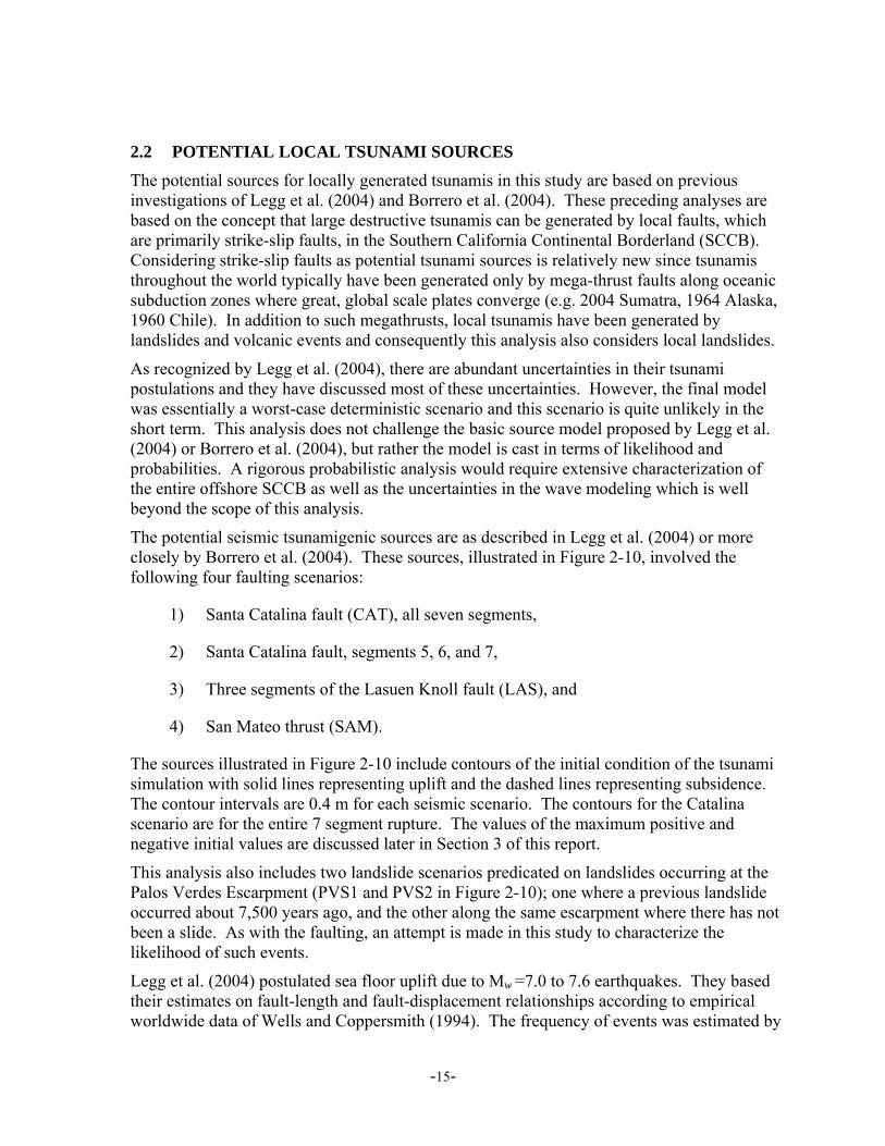
2.2 POTENTIAL LOCAL TSUNAMI SOURCES The potential sources for locally generated tsunamis in this study are based on previous investigations of Legg et al. (2004) and Borrero et al. (2004). These preceding analyses are based on the concept that large destructive tsunamis can be generated by local faults, which are primarily strike-slip faults, in the Southern California Continental Borderland (SCCB). Considering strike-slip faults as potential tsunami sources is relatively new since tsunamis throughout the world typically have been generated only by mega-thrust faults along oceanic subduction zones where great, global scale plates converge (e.g. 2004 Sumatra, 1964 Alaska, 1960 Chile). In addition to such megathrusts, local tsunamis have been generated by landslides and volcanic events and consequently this analysis also considers local landslides.

As recognized by Legg et al. (2004), there are abundant uncertainties in their tsunami postulations and they have discussed most of these uncertainties. However, the final model was essentially a worst-case deterministic scenario and this scenario is quite unlikely in the short term. This analysis does not challenge the basic source model proposed by Legg et al. (2004) or Borrero et al. (2004), but rather the model is cast in terms of likelihood and probabilities. A rigorous probabilistic analysis would require extensive characterization of the entire offshore SCCB as well as the uncertainties in the wave modeling which is well beyond the scope of this analysis.

The potential seismic tsunamigenic sources are as described in Legg et al. (2004) or more closely by Borrero et al. (2004). These sources, illustrated in Figure 2-10, involved the following four faulting scenarios:

1) Santa Catalina fault (CAT), all seven segments,

2) Santa Catalina fault, segments 5, 6, and 7,

3) Three segments of the Lasuen Knoll fault (LAS), and

4) San Mateo thrust (SAM).

The sources illustrated in Figure 2-10 include contours of the initial condition of the tsunami simulation with solid lines representing uplift and the dashed lines representing subsidence. The contour intervals are 0.4 m for each seismic scenario. The contours for the Catalina scenario are for the entire 7 segment rupture. The values of the maximum positive and negative initial values are discussed later in Section 3 of this report.

This analysis also includes two landslide scenarios predicated on landslides occurring at the Palos Verdes Escarpment (PVS1 and PVS2 in Figure 2-10); one where a previous landslide occurred about 7,500 years ago, and the other along the same escarpment where there has not been a slide. As with the faulting, an attempt is made in this study to characterize the likelihood of such events.

Legg et al. (2004) postulated sea floor uplift due to Mw =7.0 to 7.6 earthquakes. They based their estimates on fault-length and fault-displacement relationships according to empirical worldwide data of Wells and Coppersmith (1994). The frequency of events was estimated by

-16-

assuming a 1 mm/yr slip rate and dividing the displacements typical of M ~ 7.0 to 7.6 earthquakes. These procedures are commonly used by the geologic community for estimating earthquake magnitudes and recurrences when there are no specific data on specific faults or specific earthquakes. Based on these methods they estimated that tsunamis could be generated every few hundred to a few thousand years. They briefly discuss landslides and conclude they are probably less frequent than major earthquakes.

Figure 2-13 Tsunamigenic Sources from Borrero et al. (2004)

It should be pointed out that even though Legg et al. (2004) and Borerro et al. (2004) discussed various earthquake magnitudes and recurrence periods, the modeled tsunamis were not based on any probability analysis; that is, the big event is assumed to be possible but with no timetable. Large earthquakes occur every year worldwide but very few of them cause tsunamis. Such rare events should be considered on the basis of their likelihood of occurrence. Because resources with which to construct public works are finite, it behooves public agencies to put available funds to their best use, i.e. for protecting against hazards that have a realistic chance of occurring within the foreseeable future.

2.2.1 Geologic Setting The Los Angeles region lies near the junction of two major geological provinces, the Transverse Ranges (TR) and the Peninsular Ranges (PR) (Figure 2-11). The offshore area west of the Peninsular Ranges is referred to as the Southern California Continental

-17-

Borderland (SCCB) (Shepard and Emery, 1941). The SCCB has all the typical aspects of the PR but is largely underwater. The SCCB comprises the area from the Transverse Ranges on the north, represented by the Santa Barbara Channel, Channel Islands (Santa Cruz, Santa Rosa Island), and Santa Monica Mountains, to well south of the U.S./Mexico border, a distance of about 350 km. Westerly, the SCCB extends ~230 km to the Patton Escarpment where the seafloor drops off steeply to the deep Pacific abyssal plain.

Figure 2-14 Generalized and Simplified Traces of Major Faults and Provinces within

and Surrounding the Southern California Continental Borderland.

Modified from Bohannon and Geist (1998) This vast SCCB area is characterized by submarine mountains (banks) and basins. The highest mountains break the sea surface at a few locations to form islands such as Santa Catalina and San Clemente Islands. The offshore basins are commonly on the order of ~1000 m deep. The basins nearest the coastline trap sediment washed into the sea leaving the more-distant basins “starved” for terrestrial sediments and receiving only fine particles, predominantly biogenic, raining down from the water column (hemipelagic-type sediment).

-18-

At one time, the Palos Verdes Hills were one of the offshore islands and the Los Angeles Basin was one of the submarine basins. Within the past million years or so, the Los Angeles Basin has filled with sediment washed into the basin from erosion of the rising Santa Monica, San Gabriel, and Santa Ana Mountains to form the present coastal plain.

Oceanographic surveys of the SCCB reveal the basins and banks are commonly bounded by linear escarpments associated with geological faults (e.g. Vedder et al., 1974; Greene et al., 1975; Junger and Wagner, 1977). These faults form a network of braided and branching faults, and some geoscientists believe some are interrelated or interconnected forming long, continuous fault systems. If interconnected, several of these offshore fault systems would be similar in length to major onshore fault systems such as the Whittier-Elsinore and San Jacinto fault systems. The Newport-Inglewood fault of the Los Angeles Basin actually extends offshore, and along with several aligned offshore faults may be part of such a fault system interconnected with the Rose Canyon fault which extends back onshore in San Diego before extending southerly back into the offshore region toward Mexico.

Bathymetric maps of the SCCB reveal several linear ridges and escarpments and numerous hills and knolls. The linear ridges are generally associated with major faults up to a hundred kilometers or so in length (depending on how they are connected). However, the knolls are generally small with lengths of 10 or 20 kilometers and similar widths. One theory postulates that the banks and islands are uplifted due to compression along bends or step-overs in the strike-slip faults. These bends are considered to be restraining bends (see discussion under subsection entitled “Tsunami Origins and Dynamics”). There are only two large potential restraining bends in the SCCB; one along the Catalina escarpment about 50 km offshore and the other at the San Nicolas Bank about 125 km offshore (Figure 2-11). Legg et al. (2004) assumed a tsunami will occur as a result of a large earthquake on the 90-km-long restraining bend along the closer Catalina escarpment.

2.2.2 Seismological Setting Earthquake data indicate the SCCB is seismically active but at a lower level than the onshore area. Figure 2-12 is a map of earthquakes showing the distribution of M ≥ 4.0 events. The largest historical earthquakes in the offshore area are listed on Table 2-2. Undoubtedly, many small-magnitude earthquakes occurring in the SCCB are not recorded because of the large distance to seismographs. However, it is unlikely any moderate-magnitude earthquakes (M>5.0) have escaped detection. The locations of earthquakes listed in the earthquake catalog may not be very accuate because most of the seismographs are to the east providing poor azimuthal coverage that is not favorable for determining accurate locations. However, special relocating techniques (e.g. Astiz and Shearer, 2000) may reduce some of the ambiguity of the offshore seismicity distribution.

-19-

Figure 2-15 Map Showing Major Faults and Recent Seismicity (M ≥ 4) of the Southern

California Region. Some of the More Notable Events are Shown by Stars. From Legg et al., 2004.

-20-

Table 2-2 Notable Historical Earthquakes in Southern California Offshore Region

YEAR (m/d/y) MAGNITUDE LOCATION COMMENT

1/13/1877 5.0 Mexico Location highly uncertain 8/31/1930 5.2 ML Santa Monica Bay No focal mechanism; probably

reverse 3/10/1933 6.4 MW West of Newport Beach Strike-slip mechanism; relocated

onshore to Newport-Inglewood fault 5/1/1939 5.0 West of Ensenada 6/24/1939 5.0 West of Ensenada 11/14/1941 5.4 Newport Beach 2/24/1948 5.3 San Clemente Island 12/26/1951 5.9 San Clemente Island Dip-slip event 12/22/1964 5.6 West of Agua Blanca 10/24/1969 5.1 Santa Barbara Island Strike-slip 2/21/1973 5.9 ML MW Pt Mugu Thrust mechanism, dipping 36o 1/1/1979 5.2 ML MW South of Malibu Reverse mechanism, dip 60o 9/4/1981 5.5 ML 6.0MW Santa Cruz (Pilgrim) Ridge Strike slip mechanism 7/13/1986 5.3 ML West of Oceanside; north

end of San Diego Trough fault

Reverse

1/19/1989 5.0 ML MW South of Malibu Reverse

As seen in Table 2-2, there have been no large earthquakes in the SCCB in historical time. The table includes all of the known events of M ≥ 5.0. Some of the events on the list are outside the SCCB tectonic environment. Most of the events along the northern margin of the province are probably associated with thrust faults of the Western Transverse Ranges (WTR) tectonic environment. For example, the 1973 Point Mugu earthquake was clearly within the western Transverse Ranges. The 1930, 1979, and 1989 events probably occurred on east-west trending thrust faults characteristic of the western Transverse Ranges structure and not typical of the strike-slip environment of the SCCB. Regardless of their association with the WTR, they should still be considered in a tsunami hazard analysis because they are thrust faults and if large earthquakes are possible on these faults, they are probably more likely to generate tsunamis than the strike-slip faults of the SCCB.

Seismicity maps of southern California indicate earthquake activity is less frequent in the offshore area than onshore (see Figure 2-12). As discussed above, most of the activity in the Santa Monica Bay region was associated with the 1930, 1979, and 1989 events. These events are well south of the Malibu Coast fault and even south of the Santa Monica-Dume’-Anacapa fault system (Schiefelbein et al., 1998) suggesting there are unknown subsurface faults in that area (see for example, Sorlien et al., 2006). Earthquakes are relatively frequent closer to shore east of about the San Pedro Basin fault, but activity falls off farther offshore and is very low west of Catalina and San Clemente Islands. Clusters of earthquakes along

-21-

the Santa Cruz-Pilgrim Bank Ridge and along the San Clemente Escarpment are evidence of ongoing fault activity in those regions. There has been very little earthquake activity in the Catalina Island region or the San Nicolas Island region. One of the more obvious offshore features on the seismicity map is the cluster of events along the San Diego Trough fault at Krespi Knoll; these events represent the 1986 Oceanside earthquake (M=5.3) sequence.

2.2.3 Tectonic Setting In contrast to onshore faults, the offshore features have experienced relatively little earthquake activity and there has never been a large (M ≥ 7.0) earthquake in the SCCB in historical time. In spite of its relatively low rate of earthquake activity, the SCCB is commonly considered to be part of the North America-Pacific plate boundary fault system because the faults appear to have the same sense of displacement and similar trends as the major plate-bounding faults onshore. The principal faults of the plate boundary are the San Andreas and San Jacinto fault systems. Although the San Andreas in Southern California has not had a great deal of earthquake activity within historic time (i.e. the past couple hundred years) geological or “paleoseismological” trenching investigations indicate the fault has ruptured repeatedly within the past few thousand years with major events in the magnitude 7.0 to 8.0 range occurring every 100-300 years. The San Jacinto fault has been much more active seismically in historic time but with somewhat smaller events (magnitudes in the range of 6 ½ to 7 ¼). The area east of the San Andreas/San Jacinto system within the Mojave Desert and the Basin and Range area are also considered to be part of the plate-boundary fault system. These areas have numerous active faults and appear somewhat similar to the SCCB in that the topography consists of linear mountains, ridges, and valleys that are separated by young faults.

Geodetic measurements of the southern California region indicate the Pacific and North America plates slide laterally past each other at a rate of about 50 ± 2 mm/yr (Demets and Dixon, 1999; Antonelis et al, 1999). The majority of that slip budget (about 35 mm/yr) occurs along the San Andreas/San Jacinto fault system leaving about 15 mm/yr to be partitioned among all of the other remaining faults in southern California (Figure 2-16). Geologic data for major faults such as the Palos Verdes, Newport-Inglewood, and Whittier-Elsinore faults indicate slip at rates of about 3, 2, and 5 mm/yr (McNeilan et al., 1996; Lindvall and Rockwell, 1995; Rockwell et al., 1988) respectively for these faults. This takes up another 10 ± mm/yr reducing the remaining slip budget to about 5 mm/yr. Geodetic data for the Basin and Range area and the Mojave Desert (Eastern California Shear Zone) indicate as much as 11-13 mm/yr of slip (Bennet et al., 1999; Gan et al., 2000) occurs east of the San Andreas/San Jacinto fault system. The cumulative slip from just these areas accounts for more than the entire slip budget for the North America-Pacific plate displacement and leaves virtually nothing for the SCCB. There are numerous uncertainties in these types of data and it is a very complicated proposition to properly partition these global-scale crustal deformations among local faults. There are many zones of overlap as well as gaps where slip could be missed or where some may be counted twice so it is not just a simple matter of adding up all the slip on every fault. Also, much of the crustal deformation is taken up in plastic deformation (i.e. folding) and such deformation results in “loss” of slip, i.e. some of the geodetic slip is used-up by folding and is not necessarily released as fault slip. In view of

-22-

Figure 2-16 Sketch Map Showing Slip Rates on Major Faults in Southern California.

The numbers are slip rates in millimeters per year. these constraints and limitations, it is clear the geodetic data alone might not completely account for all of the active faulting. Moreover, seismcity data show earthquakes occurring in areas where there are no known faults indicating slip is occurring on other unknown faults in the region. Ward (1994) found that up to about 40 percent of the seismic moment in southern California is not associated with known surface faults.

Considering the uncertainties in adding up measured slip rates, it seems reasonable that not all of the slip budget is used up for onshore faults and some slip can reasonably be attributed to the faults within the SCCB. Even though the slip budget can be completely accounted for by onshore faults, as discussed above, the small amount of earthquake activity in the offshore area reveals that some slip must occur on faults therein.

Rates of as much as 10 or 11 mm/yr have been proposed for the SCCB (Demets and Dixon, 1999; Sella et al., 2002), and about 4 to 7 mm/yr have been postulated for the San Clemente Island fault alone (Legg, 1985). Judging whether such large amounts of slip are reasonable

-23-

on the offshore faults is difficult because reliable geodetic measurements in the offshore area are very limited owing to there being only a few islands upon which to maintain survey monuments.

Other geodetic data such as the GPS and VLBI indicate slip-velocity vectors for offshore sites are not much greater than nearby onshore sites (Fiegl et al., 1993). This indicates there is not a lot of relative displacement between the offshore region and the onshore coastal region and, therefore, the offshore region may have significantly less tectonic activity than the onshore area. In other words, the onshore region takes up most of the relative displacement leaving only a little for the offshore region.

Another way to evaluate rates of tectonic activity is by calculating strain rates and seismic moment from GPS data. Ward (1994), using the Kostrov (1974) formula, calculated strain rates for the various seismotectonic sources in southern California. This type of analysis reveals strain rates for the onshore region are much greater than for the SCCB. The Mojave Desert (Eastern California Shear Zone), for example, has strain rates about twice that of the Inner SCCB and the outer SCCB has even less. These types of data, like the historical seismicity data, indicate the SCCB has a much lower seismic potential than the onshore areas. The significance of this finding is that the offshore faults cannot be directly equated to the onshore faults, and hence the slip rates should be slower and the recurrence intervals should be longer for offshore faults, which in turn indicates less potential for large earthquakes that could cause tsunamis.

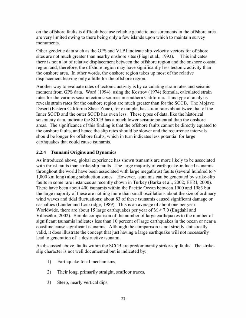
2.2.4 Tsunami Origins and Dynamics As introduced above, global experience has shown tsunamis are more likely to be associated with thrust faults than strike-slip faults. The large majority of earthquake-induced tsunamis throughout the world have been associated with large megathrust faults (several hundred to > 1,000 km long) along subduction zones. However, tsunamis can be generated by strike-slip faults in some rare instances as recently shown in Turkey (Barka et al., 2002; EERI, 2000). There have been about 400 tsunamis within the Pacific Ocean between 1900 and 1983 but the large majority of these are nothing more than small oscillations about the size of ordinary wind waves and tidal fluctuations; about 83 of these tsunamis caused significant damage or casualties (Lander and Lockridge, 1989). This is an average of about one per year. Worldwide, there are about 15 large earthquakes per year of M ≥ 7.0 (Engdahl and Villaseñor, 2002). Simple comparison of the number of large earthquakes to the number of significant tsunamis indicates less than 10 percent of large earthquakes in the ocean or near a coastline cause significant tsunamis. Although the comparison is not strictly statistically valid, it does illustrate the concept that just having a large earthquake will not necessarily lead to generation of a destructive tsunami.

As discussed above, faults within the SCCB are predominantly strike-slip faults. The strike-slip character is not well documented but is indicated by:

1) Earthquake focal mechanisms,

2) Their long, primarily straight, seafloor traces,

3) Steep, nearly vertical dips,

-24-

4) Orientations which are subparallel to active onshore strike-slip faults, and

5) A few cases of apparent right-lateral offset of submarine canyons.

The southern margin of the Western Transverse Ranges does have south-verging thrust faults (Yerkes and Lee, 1979; Fisher et al., 2005; Sorlien et al., 2006) that could represent tsunami sources. The Dume’ fault for example, is a north-dipping thrust fault. Earthquake focal mechanisms in the Western Transverse Ranges are predominantly thrust-type earthquakes but they commonly have a small component of oblique slip with a left-lateral sense of motion (Lee et al., 1979). It has long been thought there might be a slow westerly migration of the Western Transverse Ranges and this might be due to the strong north-south regional compression related to the “Big Bend” of the San Andreas Fault. This westerly migration has been termed “escape tectonics” by Walls et al. (1998). Some local geoscientists have suggested the major range-bounding Hollywood and Santa Monica faults are primarily strike-slip faults rather than reverse or thrust faults. This suggestion seems to have gained acceptance by much of the geologic community and is included in many tectonic models. If these faults are indeed primarily strike-slip, they might not pose a great tsunami potential. A scenario was evaluated in this study for the Anacapa-Dume’ and Santa Monica faults as reverse faults striking E-W, dipping 55o N with a length of 40 km. These scenarios did not generate a significant tsunami at POLA/POLB. Apparently POLA and POLB seem to be protected from local events to the north by the Palos Verdes Peninsula.

The submarine terrain in the SCCB comprising abundant high-standing ridges, knolls, and banks suggests some process other than just lateral-slip faulting is at work. One earthquake, the 1986 Oceanside event, occurred on an unknown northwest-striking, northeast-dipping subsurface reverse fault or thrust fault at a small seafloor knoll near the north end of the San Diego Trough fault. As introduced above, this event supports the idea these knolls may be at least partly tectonically formed.

The process by which a lateral-slipping fault can generate a tsunami involves the concept of restraining bends. When a linear strike-slip fault encounters a change in trend or a bend in the fault trace, compressional or extensional forces are set up along the bend. Depending on the sense of fault displacement, uplifts or depressions are created; the compressional bends are referred to as restraining bends, and the extensional bends are called releasing bends. The compressional restraining bends result in formation of ridges, banks, and knolls, and the extensional releasing bends result in basins. An example of uplift along a restraining bed may occur just onshore along the strike-slip Palos Verdes fault where uplift of the Palos Verdes Hills has occurred in the past million years or so.

Historical seismicity in the SCCB is relatively sparse and widely spread compared to the onshore area and most of the larger events in the offshore are strike-slip earthquakes. The only reverse or thrust fault event is the 1986 Oceanside event. It is important to note that no significant tsunami was associated with the 1986 event. If this event is typical of offshore events it does not provide strong support for a significant tsunami hazard. There is only one well-documented tsunami in California caused by a local source; this was caused by the 1927 Port Arguello earthquake of M=7.3 which occurred on a reverse fault off the central California coast north of Point Conception. This event occurred in a compressional tectonic environment of the Transverse Ranges so it should not be construed to be representative of

-25-

the SCCB. The event occurred before the installation of the Caltech seismograph network, which began in 1932, so the earthquake is not well documented. However, there was documented wave runup of about 1.8 m at the “village” of Surf which is now on Vandenberg Air Force Base, about 15 km from the earthquake, and runup of about 1.2 m at Port San Luis about 50 km to the north.

Another tsunami is listed for the 1812 earthquake in the Santa Barbara area. The reports of this tsunami are highly suspect with no official recording and only a few verbal anecdotal third-party recounts many years after the event. The Earthquake History of the United States (Coffman and Von Hake, 1973) states the tsunami “should be considered as lacking adequate proof.” Interestingly, it seems the longer the time from the event, the more positive the reports of its occurrence become. Lander and Lockridge (1989) provide a more-comprehensive discussion of the 1812 event. This event, like the 1927 event was generated by earthquakes in the Western Transverse Ranges province, where the dominant mode of faulting is reverse or thrust faulting and not strike-slip faulting.

2.2.5 Earthquake and Tsunami Recurrence There are virtually no specific data on the rate of tectonic activity on the faults in the SCCB. The only way to estimate the recurrence is by indirect means such as geodesy, historical seismicity, and comparison to areas with similar tectonics. As discussed above, the activity rates of historical seismicity indicate the frequency of earthquakes in the offshore region is less than onshore. This of course does not mean that large events cannot occur offshore, but that the recurrence intervals should be longer.

The lack of large earthquakes within the SCCB in itself indicates a lower level of seismicity. The great length of faults in the area, if interconnected, suggests large earthquakes could occur. Because there are no specific-slip rate or recurrence data on specific faults in the area, one has to use worldwide empirical fault length-earthquake magnitude data (e.g. Wells and Coppersmith, 1994) to estimate the size of earthquakes possible for these faults. These relationships suggest earthquakes in the magnitude 7.0 to 7.5 range are indeed possible if the faults are interconnected into long features. Seismic hazard evaluations for POLA/POLB (Earth Mechanics Inc., 2006a, 2006b) have found the earthquakes controlling seismic design at the Ports are likely to be generated by the Palos Verdes and Newport-Inglewood faults; the largest events estimated to be M=7.2. The recurrence for these events, based on geological studies, ranged from about a thousand years to a couple thousand years. This provides a starting point for comparison of offshore potential to onshore.

To evaluate the likelihood of a large earthquake occurring in the offshore area the probabilities of earthquake recurrence must be quantified. The methodology used in most probabilistic seismic hazard analyses is to characterize the earthquake recurrence relationship for each earthquake source. A recurrence relationship indicates the chance of earthquakes of a range of magnitudes occurring anywhere in the source during a specified period of time. This step is fundamentally different from a deterministic analysis where only one controlling earthquake (generally the largest conceivable event) is chosen without any consideration given to the time interval.

Gutenberg and Richter (1954) noted that earthquake magnitude and frequency appeared to have a systematic exponential relationship whereby earthquakes of one magnitude unit were

-26-

about ten times as frequent as those of a larger magnitude. This was expressed as the equation

bMaN −=10log

where

N = Annual rate of the number of earthquakes of a given magnitude M or greater,

a = Constant representing the level of seismic activity, and

b = Ratio of small to larger events

When plotted as an x-y graph with a semi-logarithmic scale, the recurrence relationships between the number of earthquakes (N) of a certain magnitude (M) plot as nearly straight lines and the b-value represents the slope of the line. This relationship is illustrated in Figure 2-17 where the earthquake recurrence curve is plotted. The b-value is a coefficient representing the relative proportion of events of different magnitude, that is, a line with a slope of -1.0 represents a recurrence relationship which for each magnitude 5 event per year, there will be one magnitude 6 event every 10 years, and one magnitude 4 earthquake every 0.1 year (or 10 magnitude 4 events every year), and so on. The a-value is a coefficient representing the intercept of the recurrence line at M=0. When b-values are the same, lines with higher a-values represent higher levels of seismicity. Historically, in areas with limited earthquake records, seismologists use the smaller more abundant earthquakes (say in the M = 3 to 5 range) to “anchor” the recurrence relationship and then extrapolate the recurrence line to estimate the frequency of larger magnitude earthquakes. Decades of earthquake observations have shown that b values generally are in the range of -0.85 to -1.1 with an average value of about –1.0.

Plotting the historical earthquake recurrence relationships as described above for all historical events over the past 70-some years within the SCCB indicates a magnitude 7.5 event can be expected about once every 14,600 years. This same recurrence relationship would yield a return period of about 4,000 years for magnitude 7.0 events and a little more than 1,000 years for magnidtude 6.5 earthquakes. The b-values for the recurrence relationships were in the range of 1.14 to 1.31. These b-values are slightly greater than worldwide averages which are about 1.0 (±0.1). To test the sensitivity of the relationships a b-value was arbitrarily assigned a value of 1.0 and anchored at the M=4.5 to 5.5 range for SCCB historical events. This exercise suggested a shorter recurrence interval of about 5,000 years for M = 7.5. Realizing that the earthquake record could be incomplete we suggest using a rounded-off recurrence interval for M=7.5 between the two calculated values, say 10,000 years. It should be emphasized there is no certainty that any of these earthquake events would result in a tsunami since as previously discussed only about 10 percent of large earthquakes in the ocean or near a coastline worldwide result in a tsunami.

-27-

Figure 2-17 Earthquake Recurrence Interval based on Earthquake Magnitude

2.2.6 Submerged Landslides

Recent tsunamis throughout the world seem to have become increasingly associated with submarine landslides. A well-known example occurred with the 1964 Alaska earthquake (Mw = 9.4) which triggered several landslides. A devastating tsunami in Papua, New Guinea in 1998 seemed anomalous for the size of the earthquake it was associated with. Subsequent investigations (e.g. Kawata, et al., 1999) found evidence indicating a large landslide may have been instrumental in the Papua tsunami. Such events have kindled interest in the role landslides play in the generation of tsunamis, but the science of predicting or modeling tsunamis from landslides is in its infancy and suffers from lack of data.

Most tsunami-generation models assume a rigid block slide (Grilli and Watts, 1999) but some numerical models (Jiang and Leblond, 1993) consider other modes of sliding. Lee et al. (2003) documents several landslides and their role in generating tsunamis. These landslides were in Alaska and the Pacific Northwest (Seattle-Tacoma). Both of these

-28-

features are believed to have generated historic tsunamis from failure of alluvial/deltaic type sediments. In general, the magnitude of tsunamis generated by submarine landslides is a function of (e.g. Murty, 1979; Harbitz, 1992; Tinti and Bortolucci, 2000):

1) Seafloor geometry,

2) Initial volume of the slide mass,

3) Extent to which the slide mass remains intact,

4) Initial acceleration, and

5) Velocity.

Large landslides in the offshore area of southern California have not been common (Legg et al., 2004), but a few have been documented (Clarke et al., 1995). Some of the reasons for the paucity of submarine landslides may be:

1) The arid climate of southern California where runoff is seasonal and buildup of sediments on submarine slopes is slow,

2) The weathering processes that break down rocks into the soil needed to create thick buildups of seafloor sediments are very slow,

3) Abundant earthquakes that occur frequently enough to set off unstable slopes on a regular basis before they have a chance to build up great thicknesses, and

4) Most terrestrial (i.e. onshore) sediment is trapped within the flatter slopes of the nearshore area leaving the vast majority of steeper slopes to the coastal basins “starved” for thick sediments.

These conditions are in marked contrast to areas such as the Pacific Northwest, Alaska, New Guinea, and Sumatra which are all areas of abundant precipitation where large amounts of sediments are washed onto steep nearshore slopes.

One large submarine landslide has been well documented in the southern California region. This feature is called the Palos Verdes debris avalanche and is clearly seen on multibeam echosounder (MBES) images of the seafloor. The feature appears to have originated on the San Pedro slope just offshore from the southwestern Palos Verdes Hills. The slope where the slide originated is a dip slope in sedimentary rocks of Pliocene and Miocene age. Interestingly, the slide occurred just offshore of the great onshore Portuguese Bend-Abalone Cove-Point Fermin (and others) landslide complex. Normark et al. (2004) and Locat et al (2004) estimated the size of this slide mass to be about 0.5 to 0.8 km3. The blocky nature of the seafloor deposit is quite clear on both seismic-reflection and MBES data. Relief of some blocks within the mass appears to be about 20 m high (Normark et al., 2004). This slide traveled over a distance of nearly 10 km down a slope of 10 to 17 degrees. The more mobile part of the avalanche spread into the San Pedro basin and left a deposit about 10 to 15 m thick.

-29-

Carbon 14 dating indicates the slide occurred about 7,500 years ago. This would place it within the time interval of rising sea level associated with the waning Pleistocene ice age. If this feature did generate a tsunami, there is probably no onshore evidence of it because the shoreline at the time is now underwater.

The mechanics of the failure are described in detail by Locat et al. (2004) and are not repeated herein. Their analysis indicates a ground acceleration of about 0.3 to 0.4g would have been enough to cause the slide. The nearest potentially active faults are the Palos Verdes, San Pedro Basin, San Pedro Escarpment, and Cabrillo faults. Both the Palos Verdes and the San Pedro Basin faults are large enough to generate M ≥ 7 earthquakes but the San Pedro Escarpment and Cabrillo faults probably are not large enough. The San Pedro Basin fault is probably too far away (15 km) to generate strong enough ground motions. Even though the San Pedro Escarpment fault may not be capable of generating earthquakes larger than about magnitude 6.5, it is very close (~ 1 km) to the San Pedro slope and even a moderate-magnitude earthquake at that distance could generate ground motions in the 0.3 to 0.4g range. It should be emphasized that the unknown parameter in the case of any historical landslide is the velocity of the slide down the slope which has a controlling impact on the creation of a tsunami based on all of the existing research on tsunami creation.

The foregoing discussion indicates there is a potential for large submarine landslides that might be able to generate a tsunami so they are included in this tsunami analysis. The tsunami analysis includes two submarine landslide scenarios; one scenario assumes reoccurrence of the landslide at the San Pedro slope where the ancient slide occurred and the other scenario assumes a similar occurrence but at another nearby location along the San Pedro slope where no previous failures are known. The second scenario is closer to POLA/POLB and therefore, should represent close to the maximum event, or basically the worst-case landslide scenario.

The available evidence indicates such tsunamigenic landslides would be extremely infrequent and probably occur less often than large earthquakes. This suggests recurrence intervals for such landslide events would be longer than the 10,000-year recurrence interval estimated for M = 7.5 earthquakes discussed above. It appears recurrence intervals for tsunami-generating slides on the order of about 10,000 years would be reasonable.

-30-

3.0 HYDRODYNAMIC MODEL DEVELOPMENT A Boussinesq wave model, MIKE21-BW, was used in this investigation to provide detailed tsunami propagation into POLA/POLB including maximum water levels, water level time histories, travel times, current speeds, and overtopping volumes. The model was configured to represent the southern California coastal area incorporating the Ports.

3.1 MIKE 21 - BW MODEL DESCRIPTION The MIKE21-BW model was developed by the Danish Hydraulic Institute (DHI, 2006), and is based on the numerical solution of the two-dimensional Boussinesq equations. The Boussinesq equations include non-linearity as well as frequency dispersion. The model is capable of reproducing the combined effects of most wave phenomena of interest in coastal and harbour engineering. These include shoaling, refraction, diffraction and partial reflection of irregular short-crested and long-crested finite-amplitude waves propagating over complex bathymetries.

3.2 BENCHMARK TEST A benchmark test case was performed to evaluate the MIKE21-BW model applicability for tsunami modeling. This benchmark problem is a 1/400 scale laboratory experiment, using a large-scale tank (205 m long, 6 m deep and 3.4 m wide) at the Central Research Institute for Electric Power Industry (CRIEPI) in Abiko, Japan (Matsuyama 1993). This physical model test has been identified as a standard benchmark tsunami modeling case in the third international workshop on long wave runup models.

Figure 3-1 shows the bathymetry used in the laboratory experiment and MIKE21-BW model. The south and north boundaries in Figure 3-1 are reflective vertical sidewalls. The incident wave from offshore (West boundary in Figure 3-1), at the water depth d = 13.5 cm, is given and shown in Figure 3-2. The primary theme of this benchmark problem is the temporal and spatial variations of the shoreline location, as well as the temporal variations of the water-surface variations at one or two specified nearshore locations. The experimental condition and data are summarized in Table 3-1.

Table 3-1 Benchmark Test Condition Summary

Bathymetry Area: 5.448m X 3.402m Minimum depth: 0.125m (land) Maximum depth: -0.13535m (water) Grid size: 0.014m

Boundary Conditions West: input wave North, East & South: solid wall

Input Wave Data Duration: 0 - 22.5sec Time step: 0.05sec Input wave data: Figure 3-2

Output Water-surface variations shown in Figure 3-3

-31-

The numerical model setup is identical to the physical model test conditions summarized in Table 3-1. Wave absorption was applied along the west edge of the basin where the incident wave was applied at the boundary while the side boundaries were setup as reflecting walls similar to the physical model basin.

Figure 3-1 Bathymetry of Benchmark Test

-0.015

-0.010

-0.005

0.000

0.005

0.010

0.015

0.020

0 5 10 15 20 25

Time (s)

Wat

er L

evel

(m)

Figure 3-2 Boundary Input Water Levels Benchmark Test

-32-

Gage 1

Gage 2

Gage 3

Gage 1

Gage 2

Gage 3

Figure 3-3 Benchmark Test Output Gage Locations

Water surface elevations were extracted from the numerical modeling results at three gage locations shown in Figure 3-3, and were compared with the water elevations measured from the physical model test. The numerical modeling results compared well with the physical model tests as shown in Figures 3-4 to 3-6. These results suggest the model is suitable for simulating the hydrodynamics of tsunami propagation into coastal areas.

-2

-1

0

1

2

3

4

5

0 5 10 15 20 25

Time (Second)

Wat

er L

evel

(cm

)

Physical Model

MIKE21-BW

Figure 3-4 Water Level Comparison at Gage 1

-33-

-2

-1

0

1

2

3

4

5

0 5 10 15 20 25

Time (Second)

Wat

er L

evel

(cm

)Physical Model

MIKE21-BW

Figure 3-5 Water Level Comparison at Gage 2

-1

0

1

2

3

4

5

0 5 10 15 20 25

Time (Second)

Wat

er L

evel

(cm

)

Physical Model

MIKE21-BW

Figure 3-6 Water Level Comparison at Gage 3

-34-

3.3 MODEL SETUP FOR POLA/POLB The MIKE21-BW model was configured to represent the southern California coastal area incorporating POLA/POLB. The model boundary extended over an area approximately 22 km by 11 km with a uniform grid spacing of 10 m with the offshore boundary near the 40 m depth contour. The latitude and longitude at the southwest corner of the modeling domain are N33.676745 and E118.321466 degrees. The model bathymetry is based on NOAA charts 18749 and 18751 (NOAA 2004a, 2004b). The model domain and bathymetry are shown in Figure 3-7. The vertical datum for the bathymetry is NGVD29 (National Geodetic Vertical Datum 1929).

Figure 3-7 MIKE21-BW Model Bathymetry

Since all of the potential sources were too far from the Ports to be practically incorporated within the detailed Boussinesq wave model due to computational limitations, the initial waves were propagated to the open water boundaries of the Boussinesq wave model using the Method of Splitting Tsunami model (MOST) after Titov and Gonzalez (1997). (The details of the initial tsumani generation are discussed in more detail in section 3.4 of this report). The southern boundary was divided into eight segments in order to simulate the differential phasing of arriving waves. The boundary input water levels in each of the eight segments are present in Figures 3-8 through 3-14 for four local tectonic tsunami sources, two local landslide tsunami sources, and one trans-ocean tsunami source. The segments are numbered from west to east or along the direction of the x-axis.

Since no model calibration data are available for tsunami wave propagation into POLA/POLB, the model parameters were configured to give minimal wave damping thereby providing conservative or upper limit results for water levels and currents. These parameters included setting the bottom friction to zero and the wave reflections off landforms to the maximum possible while retaining numerical stability. Previous experience with applying this model to POLA/POLB and calibrating against measured wave data indicate the overall applicability of the model formulation to POLA/POLB (DHI 2006).

-35-

-2

-1.5

-1

-0.5

0

0.5

1

1.5

2

12:00 12:09 12:18 12:27 12:36 12:45 12:54 13:03 13:12 13:21 13:30 13:39 13:48 13:57

Time (Earthquake starts at 12:00 pm)

Am

plitu

de (m

)South 1South 2South 3South 4South 5South 6South 7South 8

Figure 3-8 Boundary Input for the Catalina Fault - 7 Segments Scenario

-2

-1.5

-1

-0.5

0

0.5

1

1.5

2

12:00 12:09 12:18 12:27 12:36 12:45 12:54 13:03 13:12 13:21 13:30 13:39 13:48 13:57

Time (Earthquake starts at 12:00 pm)

Am

plitu

de (m

)

South 1South 2South 3South 4South 5South 6South 7South 8

Figure 3-9 Boundary Input for the Catalina Fault - 4 Segments Scenario

-36-

-1

-0.5

0

0.5

1

12:00 12:09 12:18 12:27 12:36 12:45 12:54 13:03 13:12 13:21 13:30 13:39 13:48 13:57

Time (Earthquake starts at 12:00 pm)

Am

plitu

de (m

)South 1South 2South 3South 4South 5South 6South 7South 8

Figure 3-10 Boundary Input for the Lasuen Knoll Fault Scenario

-1

-0.5

0

0.5

1

12:00 12:09 12:18 12:27 12:36 12:45 12:54 13:03 13:12 13:21 13:30 13:39 13:48 13:57

Time (Earthquake starts at 12:00 pm)

Am

plitu

de (m

)

South 1South 2South 3South 4South 5South 6South 7South 8

Figure 3-11 Boundary Input for the San Mateo Thrust Fault Scenario

-37-

-2

-1

0

1

2

12:00:00 12:09:00 12:18:00 12:27:00 12:36:00 12:45:00 12:54:00 13:03:00 13:12:00 13:21:00 13:30:00 13:39:00 13:48:00 13:57:00

Time (Earthquake starts at 12:00:00 pm)

Am

plitu

de (m

)

South 1South 2South 3South 4South 5South 6South 7South 8

Figure 3-12 Boundary Input for the Palos Verdes Landslide I Scenario

-5

-4

-3

-2

-1

0

1

2

3

4

5

12:00:00 12:09:00 12:18:00 12:27:00 12:36:00 12:45:00 12:54:00 13:03:00 13:12:00 13:21:00 13:30:00 13:39:00 13:48:00 13:57:00

Time (Earthquake starts at 12:00:00 pm)

Am

plitu

de (m

)

South 1South 2South 3South 4South 5South 6South 7South 8

Figure 3-13 Boundary Input for the Palos Verdes Landslide II Scenario

-38-

-0.3

-0.2

-0.1

0

0.1

0.2

0.3

0.4

0.5

13:30:00 15:00:00 16:30:00 18:00:00 19:30:00 21:00:00

Time (Earthquake starts at 12:00:00 pm)

Am

plitu

de (m

)

South 1

South 2

South 3

South 4

South 5

South 6

South 7

South 8

T = 3048 s = 51 min

Figure 3-14 Boundary Input for Cascadia Mw=9.2 Scenario

3.4 INITIAL TSUNAMI GENERATION AT THE SOURCES The boundary conditions for the detailed tsunami propagation model into POLA/POLB were generated by the tsunami model MOST (Titov and Synolakis, 1998, Titov and Gonzalez, 1997) coupled with four local tectonic tsunami sources and two local landslide tsunami sources. The tectonic sources are computed using an elastic deformation model based on Okada (1985). The landslide generated tsunami sources are based on empirical formula derived from the literature and from laboratory experiments on water wave generation from 3-dimensional sliding masses (Liu et al., 2005, Raichlen and Synolakis, 2003). A detailed description of the seismology and geology behind the selected scenarios is described in section 2.2 Potential Local Tsunami Sources and also given in Legg et al. (2004) and Borrero et al. (2004). In addition to the local sources, a remote source, the Cascadia Subduction Zone, was also included in this investigation as this source has received recent attention as a possible tsunamigenic area (Satake et al., 2003) and may be of potential concern for southern California.

The four local faulting scenarios used to generate initial conditions are given in Table 3-2 Two scenarios are based on the Santa Catalina Fault, Segments 1-7 and Segments 5-7, one scenario using all three segments of the Lasuen Knoll Fault, and one scenario using the complete San Mateo Thrust Fault. The details of the faulting scenarios are shown in Table 3-2 and Table 3-3 and the locations of the local tsunamigenic faults and slides are previously shown in Figure 2-10.

-39-

Table 3-2 Earthquake Source Parameters for Tsunami Simulations

Fault Seg. L (km)

W (km)

Dip (deg)

Rakea

(deg) Strike (deg)

Disp. (m)

Depthb (km)

1 21.9 14.0 89 173 313 4.0 0.5 2 28.2 14.0 85 143 293 5.0 1.0 3 16.1 14.0 70 124 277 4.8 1.0 4 20.2 14.0 80 146 303 3.6 1.0 5 8.0 14.0 80 149 300 6.4 1.5 6 40.2 14.0 80 153 297 4.5 1.0

Santa Catalina Mw=7.6

7 29.7 14.0 89 166 315 4.1 0.5 1 8.8 12.8 70 135 290 1.5 0.5 2 7.9 12.2 80 135 318 3.0 0.5

Lasuen Knoll Mw = 7.1 3 10.0 12.2 80 135 316 5.0 0.5

1 5.5 12.0 45 120 293 4.0 0.5 2 11.4 12.0 45 120 322 4.0 0.5

San Mateo Thrust Mw = 7.0 3 15.0 12.0 45 120 350 4.0 0.5 a Rake of slip vector measured from downdip direction, right slip = 180° b Depth to top of fault plane below top of elastic half space.

Table 3-3 Range of Maximum Coseismic Uplift Values for Each Initial Condition

Case Positive Negative Catalina 7 seg + 2.17a m 1.17 m Catalina 4 seg + 1.43 m 1.17 m San Mateo + 2.43 m 0.32 m Lasuen Knoll + 1.74 m 1.20 m PV Slide 1 + 3.00 m 7.00 m PV Slide 2 + 3.00 m 7.00 m a This value occurred over land and did not contribute to wave generation.

The landslide scenarios simulate a tsunami generated by a slope failure on the Palos Verdes Escarpment as described by Bohannon and Gardner (2004). The locations of these landslide sources are illustrated in Figure 3-15. Bohannon and Gardner (2004) and Locat et al., (2004) give estimates for the characteristic amplitude of the wave generated by known slope failure on the Palos Verdes Escarpment. A mid-range value from these analyses was used and from estimates given by empirical relationships described in Raichlen and Synolakis (2003) and Synolakis (2003). For the initial wave, the shape was taken as an asymmetric dipole with a Gaussian profile and a hyperbolic secant profile for the transverse direction. The characteristic amplitude of the landslide generated wave is divided between the positive and

-40-

negative lobes of the dipole with 70% going to the negative and 30% for the positive. A total amplitude of 10 m is assumed with 7 m of draw down and 3 m positive wave (Table 3-2).

Figure 3-15 Location of the Local Palos Verdes Landslide Tsunami Sources

The two landslide scenarios simulated differ only in the location and orientation of the initial condition. Scenario 1 is located over the mapped slope failure described by Bohannon and Gardner (2004) while scenario 2 is located over a section of the Palos Verdes Escarpment that has not failed, but is of similar composition and morphology to sections of the escarpment that have failed. A location was chosen closer to POLA/POLB to try and place an upper bound on the potential tsunami impact from a local submerged landslide.

The only distant tsunami source scenario modeled was based on the Cascadia Subduction Zone (CSZ) which is located along the interface between the Pacific and North American tectonic plates along the coast of the Pacific Northwest. Uslu et al (2006) describe the history of the discovery of the CSZ. The CSZ hazard was first suggested by Savage et al. (1981) in a study of crustal strain in western Washington due to a locked subduction zone. Heaton and Kanamori (1984) then compared the CSZ to other more analyzed subduction zones. Atwater (1987) examined buried lowlands in western Washington and concluded they were occasioned by rapid tectonic subsidence associated with great local earthquakes. Nelson et al. (1995) calculated coseismic subsidence from past events and proposed a possible rupture length of more than 900 km. They also suggested the most recent CSZ earthquake occurred between 1690 and 1720 AD. Satake et al. (1996) showed that the year 1700 corresponds to a historically reported tsunami in Honshu, Japan and inferred that the tsunami originated along the CSZ around 5:00 (UTC) on 27 January 1700. Satake et al. (2003), then used coastal subsidence data and numerical simulations of tsunami propagation, to conclude that the earthquake was likely grater than Mw = 9.0.

-41-

The CSZ scenario selected for assessment in this investigation was an extreme scenario suggested by Satake (2003) where a Mw=9.2 seismic event occurs over a length of 1000 km, width of 100 km, and a pure thrust slip of 20 m. The MOST tsunami model boundary conditions within southern California for this scenario were derived from the NOAA’s FACTS (Facility for the Analysis and Computation of Tsunami Simulations) database to reduce the computational requirements of extending the MOST model along the entire Pacific Coast.

Initial wave heights for all scenarios were calculated using a static initial condition which assumes an instantaneous deformation of the sea surface. The wave shape is propagated across the Southern California bathymetry using the numerical model MOST, which solves the fully non linear shallow water wave equations. Time series of wave height and velocity components were recorded at locations along the boundary surrounding the detailed tsunami propagation model for POLA/POLB to be used as input for the detailed model as described in the previous section.

3.5 HYDRODYNAMIC MODEL STILL WATER LEVEL The still water datum assumed for the model simulations was taken to be constant over the duration of the model simulations at Mean Sea Level (MSL). This water level was selected since the probability of a tsunami occurring at either higher or lower water levels is approximately equal and, given the large return interval for the tsunami scenarios, it seemed unreasonable to assume any extreme high or low water level in conjunction with the tsunami.

To demonstrate the frequency of occurrence of water levels in the Ports, a tidal prediction was made at half hour intervals over a complete 19 year tidal epoch using the tidal constituents developed for POLA by NOAA. The results of this prediction were then used to develop the cumulative frequency distribution of water levels shown in Figure 3-16. The water levels shown are referenced to the Mean Lower Low Water (MLLW) datum in POLA. MSL is defined by NOAA as being 0.86 m above MLLW. Review of the cumulative frequency distribution indicates water levels are below this approximately 47% of the time. As previously indicated, the probability the water level is above or below this level is essentially equal suggesting this water level is representative of water levels in POLA./POLB.

-42-

0%

10%

20%

30%

40%

50%

60%

70%

80%

90%

100%

-1 -0.5 0 0.5 1 1.5 2 2.5

Water Level (m, MLLW)

Cum

ulat

ive

Freq

uenc

y

Figure 3-16 Cumulative Frequency Distribution of Water Levels in POLA/POLB

over a 19-year Tidal Epoch

-43-

4.0 MODEL SIMULATION RESULTS The numerical modeling results in terms of maximum water levels, water level time histories travel time from the tsunami sources, velocities, and potential overtopping quantities at selected locations are presented in this section.

4.1 MAXIMUM WATER LEVELS Predicted maximum water levels are relatively conservative, since the MIKE21-BW model assumes vertical walls regardless of water levels in excess of the deck elevations. In reality, the water level may not reach as high after exceeding the deck elevation due to distribution of the water column over a wider area due to flooding.

Figures 4-1 through 4-7 show images of maximum water levels during the approximately two hour tsunami simulation period throughout the harbor complex for each of the seven tsunami events modeled to provide an overall summary of results. For example, Figure 4-2 shows the simulated maximum water levels throughout the entire harbor complex for the Catalina 7 Segment tsunami scenario. The maximum water levels in the same image do not necessary occur at the same time. The tsunami travel time and the time of maximum water levels at selected locations are discussed in the following two sections.

It should be emphasized the color scale for contouring the maximum water levels in these figures are all the same with the exception of the Palos Verdes Landslide which has an expanded scale due to the higher expected maximum water levels. The water levels for the Palos Verdes landslide II scenario produces maximum water levels in excess of 7 m MSL in the vicinity of Pier 400, the Navy Mole, and Cabrillo Beach whereas the remainder of the scenarios produce water levels of less than approximately 3 meters which are typically well below the deck elevations within the Ports.

-44-

Water Level [m]Above 2.8

2.6 - 2.82.4 - 2.62.2 - 2.4

2 - 2.21.8 - 21.6 - 1.81.4 - 1.61.2 - 1.4

1 - 1.20.8 - 10.6 - 0.80.4 - 0.60.2 - 0.4

0 - 0.2Below 0Undefined Value

1/1/1999 12:10:00 PM, Time step: 0, Layer: 0

0.0 0.5 1.0 1.5 2.0 2.5 3.0 3.5 4.0 4.5 5.0 5.5 6.0 6.5 7.0 7.5 8.0 8.5 9.0 9.5(Units in kilometer)

0.0

0.5

1.0

1.5

2.0

2.5

3.0

3.5

4.0

4.5

5.0

5.5

6.0

6.5

7.0

(Uni

ts in

kilo

met

er)

Water Level

Figure 4-1 Maximum Water Levels for the Catalina Fault - 7 Segments Scenario

-45-

Water Level [m]Above 2.8

2.6 - 2.82.4 - 2.62.2 - 2.4

2 - 2.21.8 - 21.6 - 1.81.4 - 1.61.2 - 1.4

1 - 1.20.8 - 10.6 - 0.80.4 - 0.60.2 - 0.4

0 - 0.2Below 0Undefined Value

1/1/1999 12:10:00 PM, Time step: 0, Layer: 0

0.0 0.5 1.0 1.5 2.0 2.5 3.0 3.5 4.0 4.5 5.0 5.5 6.0 6.5 7.0 7.5 8.0 8.5 9.0 9.5(Units in kilometer)

0.0

0.5

1.0

1.5

2.0

2.5

3.0

3.5

4.0

4.5

5.0

5.5

6.0

6.5

7.0

(Uni

ts in

kilo

met

er)

Water Level

Figure 4-2 Maximum Water Levels for the Catalina Fault - 4 Segments Scenario

-46-

Water Level [m]Above 2.8

2.6 - 2.82.4 - 2.62.2 - 2.4

2 - 2.21.8 - 21.6 - 1.81.4 - 1.61.2 - 1.4

1 - 1.20.8 - 10.6 - 0.80.4 - 0.60.2 - 0.4

0 - 0.2Below 0Undefined Value

1/1/1999 12:10:00 PM, Time step: 0, Layer: 0

0.0 0.5 1.0 1.5 2.0 2.5 3.0 3.5 4.0 4.5 5.0 5.5 6.0 6.5 7.0 7.5 8.0 8.5 9.0 9.5(Units in kilometer)

0.0

0.5

1.0

1.5

2.0

2.5

3.0

3.5

4.0

4.5

5.0

5.5

6.0

6.5

7.0

(Uni

ts in

kilo

met

er)

Water Level

Figure 4-3 Maximum Water Levels for the Lasuen Knoll Fault Scenario

-47-

Water Level [m]Above 2.8

2.6 - 2.82.4 - 2.62.2 - 2.4

2 - 2.21.8 - 21.6 - 1.81.4 - 1.61.2 - 1.4

1 - 1.20.8 - 10.6 - 0.80.4 - 0.60.2 - 0.4

0 - 0.2Below 0Undefined Value

1/1/1999 12:10:00 PM, Time step: 0, Layer: 0

0.0 0.5 1.0 1.5 2.0 2.5 3.0 3.5 4.0 4.5 5.0 5.5 6.0 6.5 7.0 7.5 8.0 8.5 9.0 9.5(Units in kilometer)

0.0

0.5

1.0

1.5

2.0

2.5

3.0

3.5

4.0

4.5

5.0

5.5

6.0

6.5

7.0

(Uni

ts in

kilo

met

er)

Water Level

Figure 4-4 Maximum Water Levels for the San Mateo Thrust Fault

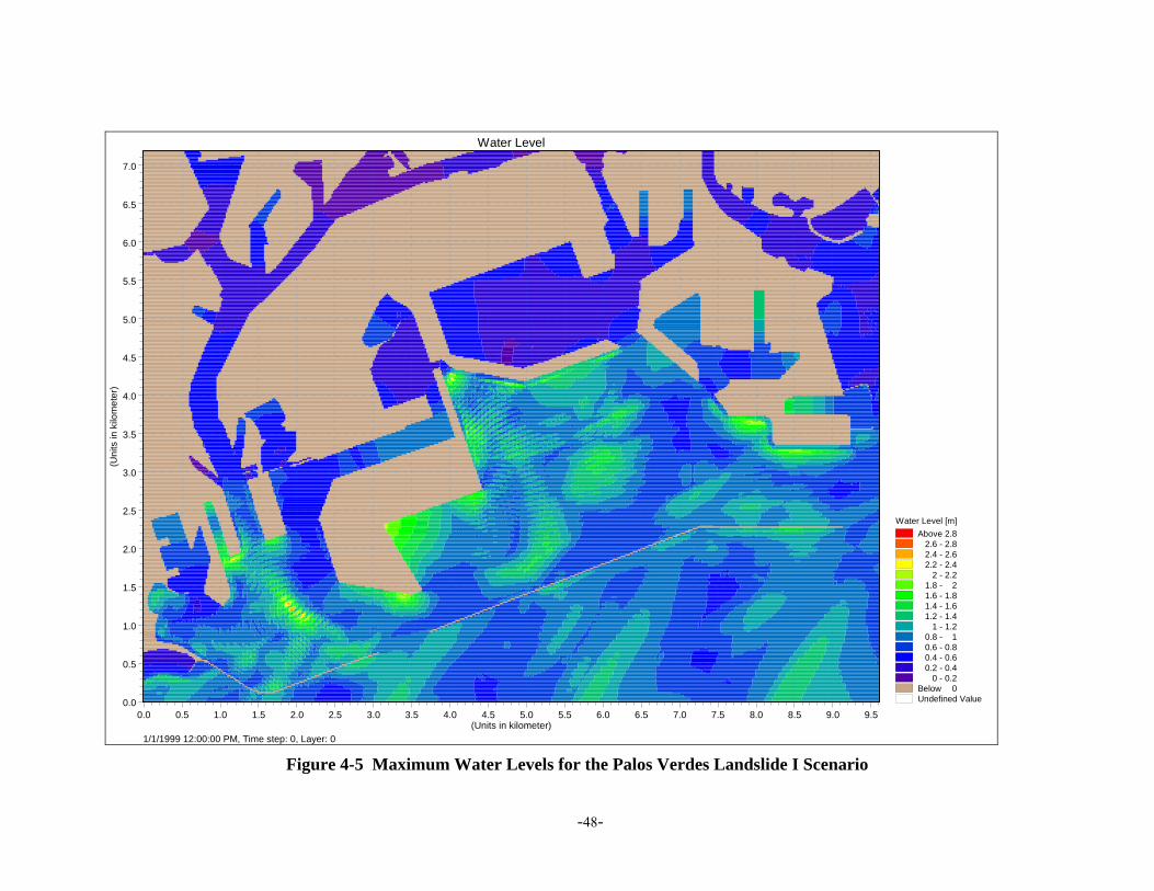
-48-

Water Level [m]Above 2.8

2.6 - 2.82.4 - 2.62.2 - 2.4

2 - 2.21.8 - 21.6 - 1.81.4 - 1.61.2 - 1.4

1 - 1.20.8 - 10.6 - 0.80.4 - 0.60.2 - 0.4

0 - 0.2Below 0Undefined Value

1/1/1999 12:00:00 PM, Time step: 0, Layer: 0

0.0 0.5 1.0 1.5 2.0 2.5 3.0 3.5 4.0 4.5 5.0 5.5 6.0 6.5 7.0 7.5 8.0 8.5 9.0 9.5(Units in kilometer)

0.0

0.5

1.0

1.5

2.0

2.5

3.0

3.5

4.0

4.5

5.0

5.5

6.0

6.5

7.0

(Uni

ts in

kilo

met

er)

Water Level

Figure 4-5 Maximum Water Levels for the Palos Verdes Landslide I Scenario

-49-

Water Level [m]Above 7

6.5 - 76 - 6.5

5.5 - 65 - 5.5

4.5 - 54 - 4.5

3.5 - 43 - 3.5

2.5 - 32 - 2.5

1.5 - 21 - 1.5

0.5 - 10 - 0.5

Below 0Undefined Value

1/1/1999 12:00:00 PM, Time step: 0, Layer: 0

0.0 0.5 1.0 1.5 2.0 2.5 3.0 3.5 4.0 4.5 5.0 5.5 6.0 6.5 7.0 7.5 8.0 8.5 9.0 9.5(Units in kilometer)

0.0

0.5

1.0

1.5

2.0

2.5

3.0

3.5

4.0

4.5

5.0

5.5

6.0

6.5

7.0

(Uni

ts in

kilo

met

er)

Water Level

Figure 4-6 Maximum Water Levels for the Palos Verdes Landslide II Scenario

-50-

Water Level [m]Above 2.8

2.6 - 2.82.4 - 2.62.2 - 2.4

2 - 2.21.8 - 21.6 - 1.81.4 - 1.61.2 - 1.4

1 - 1.20.8 - 10.6 - 0.80.4 - 0.60.2 - 0.4

0 - 0.2Below 0Undefined Value

1/1/1999 12:00:00 PM, Time step: 0, Layer: 0

0.0 0.5 1.0 1.5 2.0 2.5 3.0 3.5 4.0 4.5 5.0 5.5 6.0 6.5 7.0 7.5 8.0 8.5 9.0 9.5(Units in kilometer)

0.0

0.5

1.0

1.5

2.0

2.5

3.0

3.5

4.0

4.5

5.0

5.5

6.0

6.5

7.0

(Uni

ts in

kilo

met

er)

Water Level

Figure 4-7 Maximum Water Levels for the Cascadia Mw=9.2 Scenario

-51-

4.1.1 Maximum Water Levels in POLA In addition to the previous spatial contours of maximum water levels in POLA/POLB, maximum water levels at selected locations in POLA/POLB shown in Figure 4-8 are also tabulated in Table 4-1. The lowest deck elevations in berths adjacent to the selected gage locations are cited from Mariners Guide (POLA, 2006). The grade elevations surrounding the West Channel and in the Cabrillo Marina are based on an aerial survey performed in February 1999 and provided by the Port of Los Angeles. The grade elevation is very low in the area immediately surrounding the West Channel, and is about 1.5 m MSL. However, the adjacent buildings are set back from the waterfront and are elevated about 2.19 m above MSL. In Table 4-1, water levels exceeding the adjacent lowest deck elevation are bolded. The water level at Angels Gate is also included in the table in red to serve as a reference elevation to indicate whether waves are excited at the selected berth locations due to local resonance.

Figure 4-8 Water Level Gage Locations

As summarized in Table 4-1, the only water levels in excess of the adjacent deck elevation are for the F-face of Pier 400 for the Palos Verdes II event. The maximum water levels previously shown Figure 4-6 suggest additional areas that will be overtopped in the vicinity of Pier 400, the Navy Mole, and Cabrillo Beach for the Palos Verdes II event that are not included in the selected specific gage locations presented in Table 4-1. There are no areas with water levels in excess of the adjacent deck elevations for the other events simulated.

-52-

Table 4-1 Maximum Water Levels in Port of Los Angeles (Meters, MSL)

4.1.2 Maximum Water Levels in POLB Maximum water levels at selected locations shown in Figure 4-8 in POLB are tabulated in Table 4-2. The lowest deck elevations in berths adjacent to the selected gage locations are cited from Reference Guide and Tide Tables (POLB, 2006). The Navy Mole grade elevation is cited from a topographic map provided by the Port of Long Beach. In the table, water levels exceeding the adjacent lowest deck elevation are bolded. Water levels simulated at Queens Gate are also included in the table to serve as a reference elevation to assess whether tsunami waves are excited in the selected gage locations due to local resonance.

Table 4-2 Maximum Water Levels in Port of Long Beach (Meters, MSL)

In POLB, there are no gage locations with maximum water levels in excess of the adjacent deck elevations. The Santa Catalina 7-segment scenario produces the highest water levels for the selected gages of 3.13 m MSL at Pier J which is still less than the adjacent deck elevation of 3.59 m MSL.

-53-

4.2 WATER LEVEL TIME HISTORIES Water level time histories at the selected gage locations shown in Figure 4-8 are extracted and plotted in Figures 4-9 through 4-22 to provide detailed information on the local arrival time and the characteristics of the water level fluctuations. The deck elevation in those plots is the typical deck elevation of 3.71m, MSL (15 ft, MLLW). Deck elevations at a specific berth location are listed in Table 4-1 for the Port of Los Angeles and in Table 4-2 for the Port of Long Beach. The time scale shown assumes the tsunami starts at 12:00:00 noon.

One of the features illustrated in the time history plots is the higher frequency of the water level oscillations and substantial variability of the oscillations with location for the locally generated tsunamis compared to the lower frequency and more spatially consistent oscillations the Cascadia fault scenario which is a distant source. The Cascadia Fault results indicate a dominant wave period on the order of 50 minutes where the dominant wave period for the locally generated tsunamis indicated dominant wave periods on the order of 10 minutes and less. The uniformity of the Cascadia Fault wave period throughout the Ports suggests the offshore waters are being excited by this distant source and this offshore excitation with little damping controls the oscillations within POLA/POLB as discussed in Section 2 of this report. The variation in the magnitude of the oscillations with location for the Cascadia Fault scenario is the result of localized amplifications within the Ports.

-54-

-4.0

-3.0

-2.0

-1.0

0.0

1.0

2.0

3.0

4.0

12:09 12:18 12:27 12:36 12:45 12:54 13:03 13:12 13:21 13:30 13:39 13:48 13:57

Time (Earthquake starts at 12:00 pm)

Wat

er L

evel

s (m

, MSL

)

Pier400 FPier400 EPier400 CPier300Temp SW HabitatLA Main ChannelVT BridgeLA East BasinLA West ChannelLA East ChannelAngels GateTypical Deck Elevation

Figure 4-9 Water Levels in POLA for the Catalina Fault - 7 Segments Scenario

-55-

-2.0

-1.0

0.0

1.0

2.0

3.0

4.0

12:09 12:18 12:27 12:36 12:45 12:54 13:03 13:12 13:21 13:30 13:39 13:48 13:57

Time (Earthquake starts at 12:00 pm)

Wat

er L

evel

s (m

, MSL

)

Pier400 FPier400 EPier400 CPier300Temp SW HabitatLA Main ChannelVT BridgeLA East BasinLA West ChannelLA East ChannelAngels GateTypical Deck Elevation

Figure 4-10 Water Levels in POLA for the Catalina Fault – 4 Segments Scenario

-56-

-2.0

-1.0

0.0

1.0

2.0

3.0

4.0

12:00 12:09 12:18 12:27 12:36 12:45 12:54 13:03 13:12 13:21 13:30 13:39 13:48 13:57

Time (Earthquake starts at 12:00 pm)

Wat

er L

evel

s (m

, MSL

)

Pier400 FPier400 EPier400 CPier300Temp SW HabitatLA Main ChannelVT BridgeLA East BasinLA West ChannelLA East ChannelAngels GateTypical Deck Elevation

Figure 4-11 Water Levels in POLA for the Lasuen Knoll Fault Scenario

-57-

-2.0

-1.0

0.0

1.0

2.0

3.0

4.0

12:09 12:18 12:27 12:36 12:45 12:54 13:03 13:12 13:21 13:30 13:39 13:48 13:57

Time (Earthquake starts at 12:00 pm)

Wat

er L

evel

s (m

, MSL

)

Pier400 FPier400 EPier400 CPier300Temp SW HabitatLA Main ChannelVT BridgeLA East BasinLA West ChannelLA East ChannelAngels GateTypical Deck Elevation

Figure 4-12 Water Levels in POLA for the Santa Mateo Thrust Fault Scenario

-58-

-4

-3

-2

-1

0

1

2

3

4

12:00:00 12:09:00 12:18:00 12:27:00 12:36:00 12:45:00 12:54:00 13:03:00 13:12:00 13:21:00 13:30:00 13:39:00 13:48:00

Time ( Earthquake starts at 12:00:00)

Wat

er L

evel

s (m

, MSL

)

Pier400 FPier400 EPier400 CPier300Temp SW HabitatLA Main ChannelVT BridgeLA East BasinLA West ChannelLA East ChannelDeck ElevationAngels Gate

Figure 4-13 Water Levels in POLA for the Palos Verdes Landslide I Scenario

-59-

-4

-3

-2

-1

0

1

2

3

4

12:00:00 12:09:00 12:18:00 12:27:00 12:36:00 12:45:00 12:54:00 13:03:00 13:12:00 13:21:00 13:30:00 13:39:00 13:48:00

Time (Earthquake starts at 12:00:00)

Wat

er L

evel

s (m

, MSL

)

Pier400 FPier400 EPier400 CPier300Temp SW HabitatLA Main ChannelVT BridgeLA East BasinLA West ChannelLA East ChannelDeck ElevationAngels Gate

Figure 4-14 Water Levels in POLA for the Palos Verdes Landslide II Scenario

-60-

-0.6

-0.4

-0.2

0

0.2

0.4

0.6

1/1/1999 14:24:00 1/1/1999 15:36:00 1/1/1999 16:48:00 1/1/1999 18:00:00 1/1/1999 19:12:00 1/1/1999 20:24:00

Time (Earthquake starts at 12:00:00)

Wat

er L

evel

s (m

)

Pier400 EPier400 FPier400 CPier300Temp SW HabitatLA Main ChannelVT BridgeLA E. BasinLA W. ChannelLA E. ChannelAngels Gate

Figure 4-15 Water Levels in POLA for Cascadia Mw=9.2 Scenario

-61-

-4.0

-3.0

-2.0

-1.0

0.0

1.0

2.0

3.0

4.0

12:09 12:18 12:27 12:36 12:45 12:54 13:03 13:12 13:21 13:30 13:39 13:48 13:57

Time (Earthquake starts at 12:00 pm)

Wat

er L

evel

s (m

, MSL

)

Pier J SouthPier JLB South-East BasinLB East BasinLB Basin 6Pier T TowerPier TNear GapSouth of Navy MoleQueens GateDeck Elevation

Figure 4-16 Water Levels in POLB for the Catalina Fault - 7 Segments Scenario

-62-

-3.0

-2.0

-1.0

0.0

1.0

2.0

3.0

4.0

12:09 12:18 12:27 12:36 12:45 12:54 13:03 13:12 13:21 13:30 13:39 13:48 13:57

Time (Earthquake starts at 12:00 pm)

Wat

er L

evel

s (m

, MSL

)

Pier J SouthPier JLB South-East BasinLB East BasinLB Basin 6Pier T TowerPier TNear GapSouth of Navy MoleQueens GateDeck Elevation

Figure 4-17 Water Levels in POLB for the Catalina Fault - 4 Segments Scenario

-63-

-2.0

-1.0

0.0

1.0

2.0

3.0

4.0

12:09 12:18 12:27 12:36 12:45 12:54 13:03 13:12 13:21 13:30 13:39 13:48 13:57

Time (Earthquake starts at 12:00 pm)

Wat

er L

evel

s (m

, MSL

)

Pier J SouthPier JLB South-East BasinLB East BasinLB Basin 6Pier T TowerPier TNear GapOutside of Navy MoleQueens GateDeck Elevation

Figure 4-18 Water Levels in POLB for the Lasuen Knoll Fault Scenario

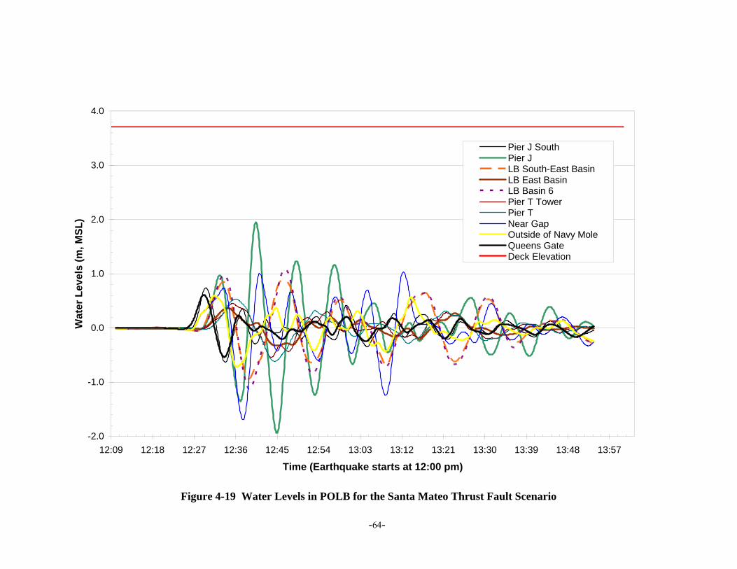
-64-

-2.0

-1.0

0.0

1.0

2.0

3.0

4.0

12:09 12:18 12:27 12:36 12:45 12:54 13:03 13:12 13:21 13:30 13:39 13:48 13:57

Time (Earthquake starts at 12:00 pm)

Wat

er L

evel

s (m

, MSL

)

Pier J SouthPier JLB South-East BasinLB East BasinLB Basin 6Pier T TowerPier TNear GapOutside of Navy MoleQueens GateDeck Elevation

Figure 4-19 Water Levels in POLB for the Santa Mateo Thrust Fault Scenario

-65-

-4

-3

-2

-1

0

1

2

3

4

12:00:00 12:09:00 12:18:00 12:27:00 12:36:00 12:45:00 12:54:00 13:03:00 13:12:00 13:21:00 13:30:00 13:39:00 13:48:00

Time (Earthquake starts at 12:00:00)

Wat

er L

evel

s (m

, MSL

)

Pier J SouthPier JLB South-East BasinLB East BasinLB Basin 6Pier T TowerPier TNear GapOutside of Navy MoleDeck ElevationQueens Gate

Figure 4-20 Water Levels in POLB for the Palos Verdes I Scenario

-66-

-4

-3

-2

-1

0

1

2

3

4

12:00:00 12:09:00 12:18:00 12:27:00 12:36:00 12:45:00 12:54:00 13:03:00 13:12:00 13:21:00 13:30:00 13:39:00 13:48:00

Time (Earthquake starts at 12:00:00)

Wat

er L

evel

s (m

, MSL

)

Pier J SouthPier JLB South-East BasinLB East BasinLB Basin 6Pier T TowerPier TNear GapOutside of Navy MoleDeck ElevationQueens Gate

Figure 4-21 Water Levels in POLB for the Palos Verdes II Scenario

-67-

-0.6

-0.4

-0.2

0.0

0.2

0.4

0.6

1/1/1999 14:24:00 1/1/1999 15:36:00 1/1/1999 16:48:00 1/1/1999 18:00:00 1/1/1999 19:12:00 1/1/1999 20:24:00

Time (Earthquake starts at 12:00:00)

Wat

er L

evel

s (m

, MSL

)

Pier J SouthPier JLB SE BasinLB E. BasinLB Basin 6Pier T TowerPier TNear GapOutside of Navy MoleNavy Basin EntranceNavy Basin NW EndNavy Basin SW EndQueens Gate

Figure 4-22 Water Levels in POLB for the Cascadia Mw=9.2 Scenario

-68-

4.3 TSUNAMI TRAVEL TIMES The tsunami travel times from their sources, which are equivalent to the possible advance warning time, are summarized in Table 4-3. For the four local tectonic tsunami sources, the travel time from each source ranges from approximately12 to 29 minutes after the earthquake. For the two local landslide tsunami sources, the travel time ranges from approximately 6 to 14 minutes depending on location within POLA/POLB. The travel time for the trans-ocean tsunami source, the Cascadia Fault is slightly over 3 hours, and the water levels caused by the trans-ocean tsunami is relatively small around 0.5 m. Table 4-3 also shows the tsunami wave periods, which provide information on what period is excited in a certain berth location.

Table 4-3 Tsunami Arrival Times and Characteristic Wave Periods

4.4 CURRENT SPEEDS IN THE CHANNELS Figure 4-23 shows selected gage locations, mainly in the navigational channels, where the depth averaged current speeds are extracted from the wave model simulations. Current speeds are calculated from model flux output. The time scales for the following time history plots is compacted The impacts of currents on berthed and moving ships can be significant and should be investigated further, but this evaluation is beyond this scope of work. In addition, there may be localized areas of scour which may be of significance to the stability of harbor breakwaters and revetments.

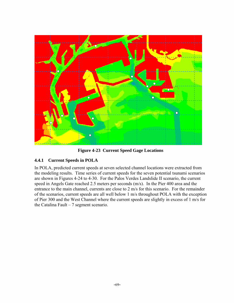
-69-

Figure 4-23 Current Speed Gage Locations

4.4.1 Current Speeds in POLA In POLA, predicted current speeds at seven selected channel locations were extracted from the modeling results. Time series of current speeds for the seven potential tsunami scenarios are shown in Figures 4-24 to 4-30. For the Palos Verdes Landslide II scenario, the current speed in Angels Gate reached 2.5 meters per seconds (m/s). In the Pier 400 area and the entrance to the main channel, currents are close to 2 m/s for this scenario. For the remainder of the scenarios, current speeds are all well below 1 m/s throughout POLA with the exception of Pier 300 and the West Channel where the current speeds are slightly in excess of 1 m/s for the Catalina Fault – 7 segment scenario.

-70-

0.0

0.5

1.0

1.5

12:09 12:18 12:27 12:36 12:45 12:54 13:03

Time (Earthquake starts at 12:00 pm)

Cur

rent

Spe

ed (m

/s)

Angels GatePier400 EPier400 CPier300LA Main Channel EntVT BridgeLA West Channel

Figure 4-24 Currents in POLA for the Catalina Fault - 7 Segments Scenario

0.0

0.2

0.4

0.6

0.8

1.0

12:09 12:18 12:27 12:36 12:45 12:54 13:03

Time (Earthquake starts at 12:00 pm)

Cur

rent

Spe

ed (m

/s)

Angels GatePier400 EPier400 CPier300LA Main Channel EntVT BridgeLA West Channel

Figure 4-25 Currents in POLA for the Catalina Fault - 4 Segments Scenario

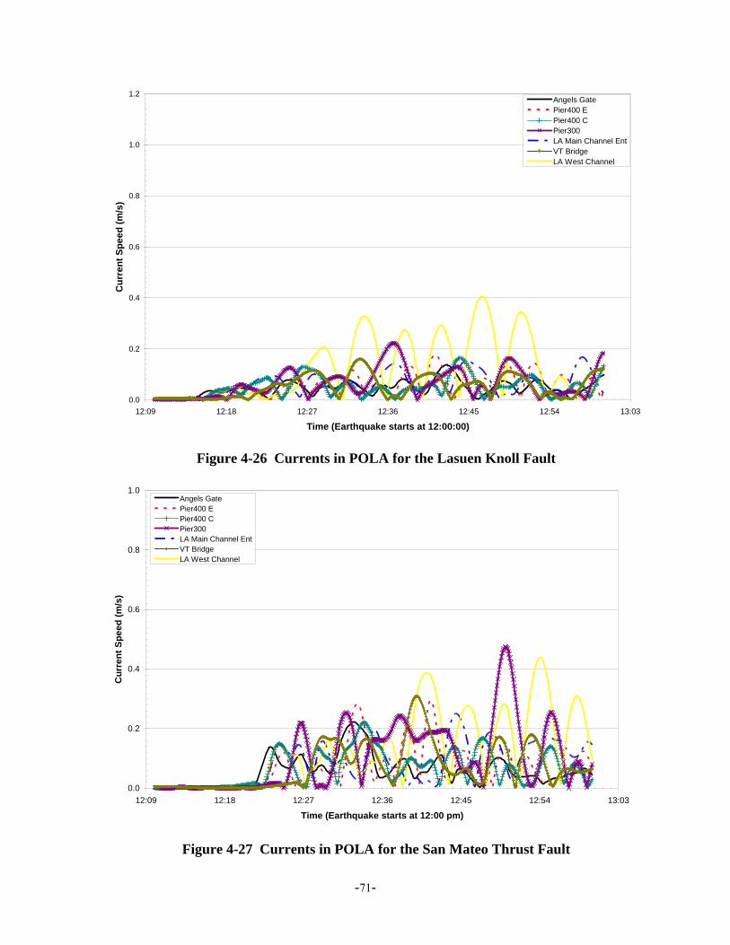
-71-

0.0

0.2

0.4

0.6

0.8

1.0

1.2

12:09 12:18 12:27 12:36 12:45 12:54 13:03

Time (Earthquake starts at 12:00:00)

Cur

rent

Spe

ed (m

/s)

Angels GatePier400 EPier400 CPier300LA Main Channel EntVT BridgeLA West Channel

Figure 4-26 Currents in POLA for the Lasuen Knoll Fault

0.0

0.2

0.4

0.6

0.8

1.0

12:09 12:18 12:27 12:36 12:45 12:54 13:03

Time (Earthquake starts at 12:00 pm)

Cur

rent

Spe

ed (m

/s)

Angels GatePier400 EPier400 CPier300LA Main Channel EntVT BridgeLA West Channel

Figure 4-27 Currents in POLA for the San Mateo Thrust Fault

-72-

0.0

0.5

1.0

1.5

2.0

2.5

3.0

12:00:00 12:09:00 12:18:00 12:27:00 12:36:00 12:45:00

Time (Earthquake starts at 12:00:00)

Cur

rent

Spe

eds

(m/s

)

Angels GatePier400 EPier400 CPier300LA Main Channel EntVT BridgeLA West Channel

Figure 4-28 Currents in POLA for the Palos Verdes I Scenario

0.0

0.5

1.0

1.5

2.0

2.5

3.0

12:00:00 12:09:00 12:18:00 12:27:00 12:36:00 12:45:00

Time (Earthquake starts at 12:00:00)

Cur

rent

Spe

eds

(m/s

)

Angels GatePier400 EPier400 CPier300LA Main Channel EntVT BridgeLA West Channel

Figure 4-29 Currents in POLA for the Palos Verdes II Scenario

-73-

0.0

0.1

0.2

0.3

0.4

0.5

0.6

14:24:00 15:54:00 17:24:00 18:54:00 20:24:00

Time (Earthquake starts at 12:00:00)

Cur

rent

Spe

eds

(m/s

)Angels GatePier400 EPier400 CPier300LA Main Channel EntVT BridgeLA West Channel

Figure 4-30 Currents in POLA for the Cascadia Mw=9.2 Scenario

4.4.2 Current Speeds in POLB In POLB, predicted current speeds at seven selected channel locations were extracted from the modeling results. Time series of current speeds for the seven potential tsunami scenarios are shown in Figures 4-31 to 4-37. The current speeds in POLB are generally higher than in POLA for all of the scenarios. In particular, the entrances to the SE Basin and the Navy Basin are consistently the locations with the highest current speeds. For the Catalina – 7 segment scenario, the current speeds at the SE Basin entrance and the Navy Basin entrance exceed 4 m/s. For the remainder of the local tsunami sources, the current speeds typically exceed 2.0 m/s in the SE Basin entrance with the exception of the Lasuen Knoll scenario where the current speeds are close to 1.0 m/s. For the remainder of the locations, almost all current speeds are less than 1.0 m/sec for all scenarios with the exception of Henry Ford Avenue and Pier J entrance where the current speeds are slightly greater than 1.0 m/s for the Catalina – 7 segment scenario.

-74-

0.0

1.0

2.0

3.0

4.0

5.0

12:09 12:18 12:27 12:36 12:45 12:54 13:03

Time (Earthquake starts at 12:00 pm)

Cur

rent

Spe

ed (m

/s)

Queens GatePier JLB SE BasinLB SE Basin Ent.LB Main ChannelNavy Basin Ent.Back ChannelHenry Fort Ave.

Figure 4-31 Currents in POLB for the Catalina Fault - 7 Segments Scenario

0.0

1.0

2.0

3.0

4.0

5.0

12:09 12:18 12:27 12:36 12:45 12:54 13:03

Time (Earthquake starts at 12:00 pm)

Cur

rent

Spe

ed (m

/s)

Queens GatePier JLB SE BasinLB SE Basin Ent.LB Main ChannelNavy Basin Ent.Back ChannelHenry Ford Ave.

Figure 4-32 Currents in POLB for the Catalina Fault - 4 Segments Scenario

-75-

0.0

0.5

1.0

1.5

2.0

12:09 12:18 12:27 12:36 12:45 12:54 13:03

Time (Earthquake starts at 12:00 pm)

Cur

rent

Spe

ed (m

/s)

Queens GatePier JLB SE BasinLB SE Basin Ent.LB Main ChannelNavy Basin EntranceBack ChannelHenry Ford Ave.

Figure 4-33 Currents in POLB for the Lasuen Knoll Fault

0.0

0.5

1.0

1.5

2.0

2.5

3.0

3.5

4.0

4.5

5.0

12:09 12:18 12:27 12:36 12:45 12:54 13:03

Time (Earthquake starts at 12:00 pm)

Cur

rent

Spe

ed (m

/s)

Queens GatePier JLB SE BasinLB SE Basin Ent.LB Main ChannelNavy Basin EntranceBack ChannelHenry Ford Ave.

Figure 4-34 Currents in POLB for the San Mateo Thrust Fault

-76-

0.0

0.5

1.0

1.5

2.0

2.5

3.0

12:00:00 12:09:00 12:18:00 12:27:00 12:36:00 12:45:00

Time (Earthquake starts at 12:00:00)

Cur

rent

Spe

eds

(m/s

)

Queens GatePier JLB SE BasinLB SE Basin Ent.LB Main ChannelNavy Basin Ent.Back ChannelHenry Ford Ave.

Figure 4-35 Currents in POLB for the Palos Verdes I Scenario

0.0

0.5

1.0

1.5

2.0

2.5

3.0

12:00:00 12:09:00 12:18:00 12:27:00 12:36:00 12:45:00

Time (Earthquake starts at 12:00:00)

Cur

rent

Spe

eds

(m/s

)

Queens GatePier JLB SE BasinLB SE Basin Ent.LB Main ChannelNavy Basin Ent.Back ChannelHenry Ford Ave.

Figure 4-36 Currents in POLB for the Palos Verdes II Scenario

-77-

0.0

0.1

0.2

0.3

0.4

0.5

0.6

14:24:00 15:54:00 17:24:00 18:54:00 20:24:00

Time (Earthquake starts at 12:00:00)

Cur

rent

Spe

eds

(m/s

)Queens GatePier JLB SE BasinLB SE Basin Ent.LB Main ChannelNavy Basin EntranceBack ChannelHenry Ford Ave.

Figure 4-37 Currents in POLB for the Cascadia Mw=9.2 Scenario

4.5 OVERTOPPING ASSESSMENT Water levels at some of the berthing locations are higher than the surrounding deck elevations. As a result, overtopping will occur in these areas. However, the tsunami wave overtopping is different from normal gravity waves of local sea and swell overtopping since tsunami wave periods are much longer and the waves don’t break and runup on structures as short period waves do. The overtopping phenomenon of tsunami waves is closer to a weir analogy. An analytical method (Takada, 1996) based on the weir method developed for standing waves overtopping sea-walls was applied in this study for calculating overtopping volumes.

For the scenarios simulated, the only overtopping expected is for the Palos Verdes II landslide scenario and the overtopping is limited to the Navy Mole area and the F face of Pier 400 based on the water level time histories previously discussed. The potential for total overtopping volumes over a unit width for these two locations is 0.40 m3/m and 1.80 m3/m for the Navy Mole area and the F face of Pier 400, respectively. The duration of each overtopping incident is very short and is less than 3 minutes. The overtopping durations for individual berths can be found in the water level time history plots in Section 4.2.

Based on the maximum water level distributions previously discussed in Section 4.1, there are additional areas where overtopping is expected for this scenario, but these areas are limited and require more detailed modeling of the overtopping and inundation that should be covered in additional analysis beyond the scope of this project.

-78-

5.0 MODEL SENSITIVITY SIMULATIONS

5.1 FEDERAL BREAKWATER SENSITIVITY In the numerical modeling of long period tsunami waves, the federal breakwaters were represented as porous structures in the bathymetry file since the long period waves will penetrate the breakwaters. The damping effect of the federal breakwater was simulated by a porosity along the structures. This section describes the sensitivity of the breakwater effect which is simulated by varying the porosity characteristics in the MIKE-21 BW model.

The Palos Verdes I scenario was selected to perform the sensitivity test. Figures 5-1 and 5-2 show the differences in water levels with and without breakwaters (labeled as No_BW in the legend for the latter). The water levels are slightly higher for the without breakwater condition. The differences are very small in the Port of Long Beach. These results suggest, the damping effect of the breakwater is relatively small, which is considered reasonable for the long period waves.

-1.5

-1.0

-0.5

0.0

0.5

1.0

1.5

12:00:00 12:09:00 12:18:00 12:27:00 12:36:00 12:45:00 12:54:00 13:03:00 13:12:00 13:21:00 13:30:00 13:39:00 13:48:00 13:57:00

Time (Earthquake starts at 12:00:00 pm)

Wat

er L

evel

s (m

)

Pier 300Pier 300 No_BWPier 400 CPier 400 C No_BWLA Main ChannelLA Main Channel No_BWVT BridgeVT Bridge No_BW

Figure 5-1 Comparison of Water Levels in POLA between With and Without Federal

Breakwaters for the Palos Verdes I Scenario

-79-

-1.5

-1.0

-0.5

0.0

0.5

1.0

1.5

12:00:00 12:09:00 12:18:00 12:27:00 12:36:00 12:45:00 12:54:00 13:03:00 13:12:00 13:21:00 13:30:00 13:39:00 13:48:00 13:57:00

Time (Earthquake starts at 12:00:00 pm)

Wat

er L

evel

s (m

)Pier JPier J No_BWLB SE BasinLB SE Basin No_BWPier TPier T No_BWNear GapNear Gap No_BW

Figure 5-2 Comparison of Water Levels in POLB between With and Without Federal

Breakwaters for the Palos Verdes I Scenario

5.2 IMPACTS OF SCALING WAVE AMPLITUDES Tsunami wave amplitudes for some scenarios are very high such as the Santa Catalina fault scenarios. These high wave amplitudes did cause numerical instabilities. To alleviate these instability problems in the hydrodynamic wave model, both Santa Catalina fault scenarios and the Palos Verdes II scenario were simulated with reduced amplitudes. The results of these model simulations were then corrected to the proper scale for analysis and presentation of the results in this report. Theoretically, scaling down the amplitude should not affect the modeling results as long as the problem is not strongly non-linear. This section discusses the potential impacts due to the amplitude scale down.

The Lasuen Knoll fault scenario is used in this exercise. The modeling results from an arbitrary wave amplitude input (called prototype scale) which is larger than the inputs used in the results discussed above were compared with those from half of the amplitude inputs (model scale). Figures 5-3 and 5-4 show water level comparisons where the water levels simulated with half of the amplitudes were multiplied by two to convert them back to the prototype scale. The results indicate water levels from both prototype and model scales are very similar. The wave amplitudes from model scale are slighter bigger than those from prototype scale which suggest results are on the conservative side. These results indicate the wave amplitude is linear for this particular application

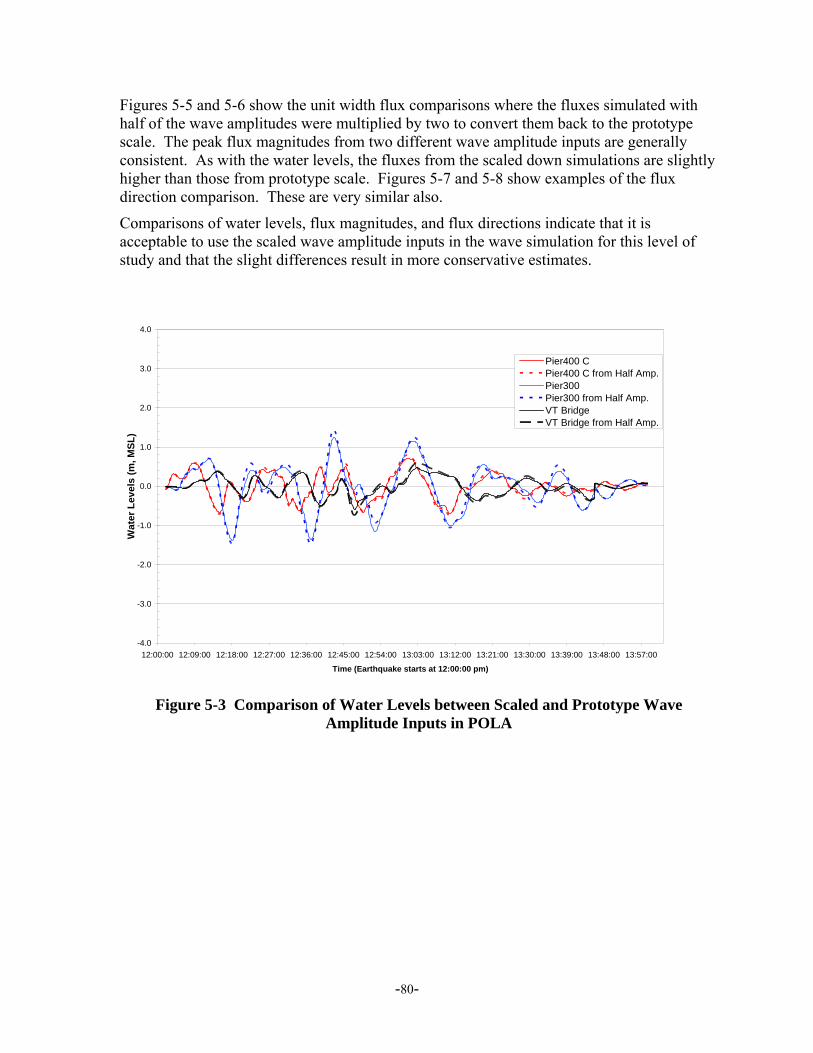
-80-

Figures 5-5 and 5-6 show the unit width flux comparisons where the fluxes simulated with half of the wave amplitudes were multiplied by two to convert them back to the prototype scale. The peak flux magnitudes from two different wave amplitude inputs are generally consistent. As with the water levels, the fluxes from the scaled down simulations are slightly higher than those from prototype scale. Figures 5-7 and 5-8 show examples of the flux direction comparison. These are very similar also.

Comparisons of water levels, flux magnitudes, and flux directions indicate that it is acceptable to use the scaled wave amplitude inputs in the wave simulation for this level of study and that the slight differences result in more conservative estimates.

-4.0

-3.0

-2.0

-1.0

0.0

1.0

2.0

3.0

4.0

12:00:00 12:09:00 12:18:00 12:27:00 12:36:00 12:45:00 12:54:00 13:03:00 13:12:00 13:21:00 13:30:00 13:39:00 13:48:00 13:57:00

Time (Earthquake starts at 12:00:00 pm)

Wat

er L

evel

s (m

, MSL

)

Pier400 CPier400 C from Half Amp.Pier300Pier300 from Half Amp.VT BridgeVT Bridge from Half Amp.

Figure 5-3 Comparison of Water Levels between Scaled and Prototype Wave

Amplitude Inputs in POLA

-81-

-4.0

-3.0

-2.0

-1.0

0.0

1.0

2.0

3.0

4.0

12:00:00 12:09:00 12:18:00 12:27:00 12:36:00 12:45:00 12:54:00 13:03:00 13:12:00 13:21:00 13:30:00 13:39:00 13:48:00 13:57:00

Time (Earthquake starts at 12:00:00 pm)

Wat

er L

evel

s (m

, MSL

)

Pier J SouthPier J South from Half Amp.LB SE BasinLB SE Basinfrom Half Amp.Pier TPier T from Half Amp.

Figure 5-4 Comparison of Water Levels between Scaled and Prototype Wave

Amplitude Inputs in POLB

0

5

10

15

20

25

1/1/1999 12:18:00 1/1/1999 12:27:00 1/1/1999 12:36:00 1/1/1999 12:45:00 1/1/1999 12:54:00 1/1/1999 13:03:00

Time (Earthquake starts at 12:00:00 pm)

Flux

(m3 /s

/m)

Pier400 CPier400 C from Half Amp.Pier300Pier300 from Half Amp.VT BridgeVT Bridge from Half Amp.

Figure 5-5 Comparison of Fluxes between Scaled and Prototype Wave Amplitude

Inputs in POLA

-82-

0

5

10

15

20

25

1/1/1999 12:18:00 1/1/1999 12:27:00 1/1/1999 12:36:00 1/1/1999 12:45:00 1/1/1999 12:54:00 1/1/1999 13:03:00

Time (Earthquake starts at 12:00:00 pm)

Flux

(m3 /s

/m)

Pier J SouthPier J South from Half Amp.Pier TPier T from Half Amp.LB South-East BasinLB South-East Basin from Half Amp.

Figure 5-6 Comparison of Fluxes between Scaled and Prototype Wave Amplitude

Inputs in POLB

0

30

60

90

120

150

180

210

240

270

300

330

360

1/1/1999 12:18:00 1/1/1999 12:27:00 1/1/1999 12:36:00 1/1/1999 12:45:00 1/1/1999 12:54:00 1/1/1999 13:03:00

Time (Earthquake starts at 12:00:00 pm)

Dirc

tion

(Tru

e N

orth

)

Pier400 C

Pier400 C from Half Amp.

Figure 5-7 Comparison of Flux Directions between Scaled and Prototype Wave

Amplitude Inputs in POLA

-83-

0

30

60

90

120

150

180

210

240

270

300

330

360

1/1/1999 12:18:00 1/1/1999 12:27:00 1/1/1999 12:36:00 1/1/1999 12:45:00 1/1/1999 12:54:00 1/1/1999 13:03:00

Time (Earthquake starts at 12:00:00pm)

Dirc

tion

(Tru

e N

orth

)Pier T

Pier T from Half Amp.

Figure 5-8 Comparison of Flux Directions between Scaled and Prototype Wave

Amplitude Inputs in POLB

-84-

6.0 CONCLUSIONS A Boussinesq wave model, MIKE21-BW, was used in this investigation to simulate the detailed tsunami wave propagation into POLA/POLB. Seven potential tsunami sources were modeled which included four local tectonic scenarios, two local submarine landslide scenarios, and one distant tsunami source scenario. The four local tectonic scenarios consisted of Santa Catalina Fault - 7 segments, Santa Catalina Fault - 4 segments, Lasuen Knoll Fault, and San Mateo Thrust Fault. The two local submarine landslide scenarios consisted of two locations offshore of Palos Verdes. The distant tsunami source scenario consisted of a tectonic event on the Cascadia Subduction Zone. The first six scenarios were considered to be representative of a wide range of potential local tsunami sources, and the last represented the potentially significant Cascadia Subduction Zone event.

The seismicity and tectonics of the Southern California Continental Borderland (SCCB) were analyzed to help characterize the potential for tsunami-generating earthquakes. The analysis indicated the SCCB has few restraining bends with thrust-type faulting sources large enough to generate significant tsunamis, and therefore tsunamis appear to be extremely infrequent. Large earthquakes (M~7.5) are very infrequent and have not occurred in the offshore area of California within historical times. Furthermore, not every large earthquake is expected to generate a tsunami based on historical occurrences of tsunamis and seismic activity throughout the world. Based on the seismicity, geodetics, and geology, a large locally generated tsunami from either local seismic activity or a local submarine landslide would likely not occur more than once every 10,000 years.

In addition to evaluation of the local tsunamigenic sources, a review was made of historical tsunamis arriving at POLA/POLB from remote sources. The primary remote sources with significant water level fluctuations were Chile and Alaska. Other remote sources do not seem to generate substantial tsunami amplitudes along the southern California coastline. This review also suggests the maximum mean wave height resulting from the identified sources is approximately 0.75 m with associated wave heights within the tsunami wave train having a Rayleigh distribution which describes the maximum expected wave height in the wave train as well. The results suggest the historically recorded tsunamis in POLA/POLB may be the maximum to be expected from remote sources.

Prior to applying the detailed tsunami propagation model to POLA/POLB, the model was configured to represent at benchmark test case based on a physical model of the Okushiri, Japan tsunami in 1993. The Boussinesq model results agreed very well with the physical model tests indicating the appropriateness of utilizing the model for simulating tsunami propagation into coastal areas.

Model results for the 7 scenarios simulated suggest the worst case scenario for POLA/POLB is for the Palos Verdes landslide II scenario. Water levels exceed adjacent deck elevations in some localized areas. Water levels are slightly in excess of 7 m along Pier 400 in POLA and along the Navy Mole in POLB. These water levels will be expected to overtop the adjacent wharves in these areas. However, for the bulk of the

-85-

area within POLA/POLB, limited overtopping is expected for this scenario and no overtopping is expected for the other scenarios.

For the four local tectonic tsunami sources, the travel time after the initial earthquake to Angels Gate in POLA ranges from 12 to 23 minutes and the travel time to Queens Gate in POLB ranges from approximately 18 to 29 minutes. For the two local landslide tsunami sources, the travel time after the initial landslide is between 6 and 9 minutes at Angels Gate and 12 to 14 minutes at Queens Gate. The travel time for the trans-ocean tsunami source, the Cascadia Subduction Zone, is slightly over 3 hours.

Current speeds in POLA can reach as high as 2.5 m/s in Angels Gate for the Palos Verdes Landslide II scenario. In the Pier 400 area and the entrance to the main channel, currents are close to 2 m/s for this scenario. For the remainder of the scenarios, current speeds are all well below 1 m/s throughout POLA with the exception of Pier 300 and the West Channel where the current speeds are slightly in excess of 1 m/s for the Catalina Fault – 7 segment scenario.

The current speeds in POLB are generally higher than in POLA for all of the scenarios. In particular, the entrances to the SE Basin and the Navy Basin are consistently the locations with the highest current speeds. For the Catalina – 7 segment scenario, the current speeds at the SE Basin entrance reach 4.1 m/s and 4.3 m/s at the Navy Basin entrance. For the remainder of the local tsunami sources, the current speeds typically exceed 2.0 m/s in the SE Basin entrance. For the remainder of the locations, almost all current speeds are less than 1.0 m/sec for all scenarios. These data should be used for evaluating impacts to berthed and moving ships as mooring forces and navigational issues may become significant.

Overtopping volumes were calculated at selected areas within POLA/POLB utilizing a broad crested weir approach. As expected, the maximum overtopping was associated with the previously described maximum water level locations for the PalosVerdes landslide II scenario.

-86-

7.0 REFERENCES

Antonelis, K., Johnson, D.L., Miller, and M.M., Palmer, R. 2002. “GPS Determination of Current Pacific-North American Plate Motion,” Geology, v. 27, p 299-302.

Astiz, L., and Shearer, P.M. 2000. “Earthquake Locations in the Inner Continental Borderland, Offshore Southern California,” Bulletin of the Seismological Society of America, v. 90, p 425-449.

Atwater, B. F. 1987. “Evidence for great holocene earthquakes along the outer coast of Washington State,” Science, 236, 942–944.

Barka, A., and others. 2002. “The Surface Rupture and Slip Distribution of the 17 August 1999 Izmit Earthquake (m 7.4), North Anatolian Fault,” Bulletin of the Seismological Society of America, v. 92, p 43-60.

Bennett, R.A., Davis, J.L., and Wernicke, B.P. 1999. “Present-Day Pattern of Cordilleran Deformation in the Western United States: Geology, v. 27, p 371-374.

Berkman, S.C., and Symons, J.M. 1964 February. “The Tsunami of May 22, 1960 as Recorded at Tide Stations”, U.S. Dept. of Commerce, Coast and Geodetic Survey.

Bohannon, R.G., and Geist, E. 1998. “Upper Crustal Structure and Neogene Tectonic Development of the California Continental Borderland,” Geological Society of America Bulletin, v. 110, p 779-800.

Bohannon, R. and Gardner, J. 2004. “Submarine Landslides of San Pedro Escarpment,” Marine Geology, 203, p 261-268.

Borrero, J.C., Legg, M.R., and Synolakis, C.E. 2004 July. “Nearshore Tsunami Sources in Southern California,” Geophysical Research Letters. Vol 31.

Borrero, J., S. Cho, J.E. Moore, H.W. Richardson, and C.E. Synalokis. 2005 April. “Could It Happen Here?” Civil Engineering, p 54-65.

Borrero, J.C., Gonzalez, F.I., Titov, V.V., Newman, J.C., Venturato, A.J., and Legg, G. 2004 December. “Application of FACTS as a tool for modeling, archiving and sharing tsunami simulation results,” Abstract and Poster, American Geophysical Union Fall Meeting, San Francisco, CA.

Clarke, S.H., Greene, H.G., and Kennedy, M.P. 1985. “Identifying Potentially Active Faults and Unstable Slopes Offshore in Evaluating Earthquake Hazards in the Los Angeles Region–an Earth-Science Perspective,” U.S. Geological Survey Professional Paper 1360, p 347-373.

Coffman, J.L., and von Hake, C.A. 1973. “Earthquake History of the United States,” U.S. Department of Commerce, National Oceanic and Atmospheric Administration, Publication 41-1, Revised Edition (Through 1970).

-87-

Demets, C., and Dixon, T.H. 1999. “New Kinematic Models for Pacific-North America Motion from 3 ma to Present, I: Evidence for Steady Motion and Biases in the NUVEL-1A Model,” Geophysics Research Letters, v. 26, p 1921-1924.

DHI Water & Environment. 2006. http://www.dhisoftware.com/Mike21/Description /m21bw/ BW_Module.htm. Accessed January 2006.

Earth Mechanics, Inc. 2006a. “Port-Wide Ground Motion and Palos Verdes Fault Study,” Port of Los Angeles, California, report under preparation for the Port of Los Angeles.

Earth Mechanics, Inc. 2006b. “Port-Wide Ground Motion Study,” Port of Long Beach, California, report under preparation for the Port of Long Beach.

EERI (Earthquake Engineering Research Institute). 2000. “Tsunami Waves in Izmit Bay: Earthquake Spectra: in 1999 Kocaeli, Turkey,” Earthquake Reconnaissance Report, v. 16, Supplement A, p 55-62.

Engdahl, E.R., and Villseñor A. 2002. “Global Seismicity: 1900-1999, in International Handbook of Earthquake and Engineering Seismology,” Academic Press for International Association of Seismology and Physics of the Earth’s Interior, p 665-690.

Feigl, K.L., Agnew, D.C., Bock, Y., Dong, D., Donnellan, A., Hager, B.H., Herring, T.A., Jackson, D.D., Jordan, T.H., King, R.W., Larsen, S., Larson, K.M, Murray, M.M., Shen, Z., and Webb, F.H. 1993. “Space Geodetic Measurement of the Velocity Field in Central and Southern California,” 1984-1992, Journal of Geophysical Research, v. 98, p 21,677-21,712.

Fischer, P.J., and Mills, G.I. 1991. “The offshore Newport-Inglewood-Rose Canyon Fault Zone, California: Structure, Segmentation, and Tectonics: in Environmental Perils of the San Diego Region,” San Diego Association of Geologists Guidebook, p 17-36.

Fisher, M.A., Langenheim, V.E., Sorlien, C.C., Dartnell, P., Sliter, R.W., Cochrane, G.R., and Wong, F.L. 2005. “Recent Deformation along the Offshore Malibu Coast, Dume, and Related Faults West of Point Dume,” Southern California: Bulletin of the Seismological Society of America, v. 95, p 2486-2500.

Gan, W., Svarc, J.L., Savage, J.C., and Prescott, W.H. 2000. “Strain Accumulation Across the Eastern California Shear Zone at Latitude 36o30’N,” Journal of Geophysical Research, v. 105, p. 16,229-16,236.

Greene H.G., Clarke, S.H., Field, M.E., Linder, F.I., and Wagner, H.C. 1975. Preliminary Report on the Environmental Geology of Selected Areas of the Southern California Continental Borderland. U.S. Geological Survey, Open-File Report 75-596.

Grilli, S.T., and Watts, P. 1999. “Modeling of Waves Generated by a Moving Submerged Body, Applications to underwater landslides,” Eng. Anal. Bound. Elem., v. 23, p 645-656.

-88-

Harbitz, C.B. 1992. “Model Simulations of Tsunamis Generated by the Storegga Slides,” Marine Geology, v. 105, p 1-21.

Heaton, T. H., and Kanamori, H. 1984. “Seismic potential associated with subduction in the Northwestern United States,” Bulletin of the Seismological Society of America, 74 (3), 933–941.188

Houston, J.R. 1980. “Type 19 Flood Insurance Study: Tsunami Predictions for Southern California.” U.S. Waterways Experimental Station, Vicksburg, Miss., available from National Technical Information Service.

Jiang, L. and Leblond, P.H. 1993. “Numerical Modeling of an Underwater Bingham Plastic Mudslide and the Waves Which It Generates,” Journal of Geophysical Research, v. 98, p 10303-10317.

Junger, A., and Wagner, H.C. 1977. “Geology of the Santa Monica and San Pedro basins, California Continental Borderland,” U.S. Geological Survey, Miscellaneous Field Studies Map MF-820.

Kanamori, H. 1977. “The energy release in great earthquakes,” Journal of Geophysical Research, Vol. 82, No. 20.

Kawata, Y., Benson, B.C., Borrero, J., Davies, H., de Lange, W., Imamura, F., Synolakis, C.E., 1999, Tsunami in Papua New Guinea, EOS, Transactions American Geophysical Union, 80 (9) 101-105. (EOS Cover Article)

Kostrov, B.V. 1974. “Seismic Moment and Energy of Earthquakes, and Seismic Flow of Rock,” Isvestia Academy of Science, USSR Physics of Solid Earth, v. 1, p 23-40.

Lander, J.G., and Lockridge. 1989. “United States Tsunamis, 1690-1988,” U.S. Department of Commerce, National Geophysical Data Center, Publication 41-2.

Lee, H.J., Kayen, R.E., Gardner, J.V., and Locat, J. 2003. “Characteristics of Several Tsunamigenic Submarine Landslides,” preprint, in press.

Lee, W.H.K., Yerkes, R.F., and Simirenko, M. 1979. “Recent Earthquake Activity and Focal Mechanisms in the Western Transverse Ranges, California: in Earthquake Activity and Quaternary Deformation of the Western Transverse Ranges, California,” U.S. Geological Survey Circular 799.

Legg, M.R. 1985. “Geologic Structure and Tectonics of the Inner Continental Borderland Offshore Northern Baja California, Mexico,” University of California, Santa Barbara, Ph.D. Dissertation.

Legg, M.R., Borrero, J.C., and Synolakis, C.E. 2004. “Tsunami Hazards Associated with the Catalina Fault in Southern California,” Earthquake Spectra, v. 20, p 917-950.

Lindvall, S.C., and Rockwell, T.L 1995. “Holocene Activity of the Rose Canyon Fault Zone in San Diego, California,” Journal of Geophysical Research, v. 100, p 24121-24132.

-89-

Liu, P. L.-F., Wu, T.-R., Raichlen, F., Synolakis, C.E., and Borrero J.C. 2005. “Runup and Rundown Generated by Three-Dimensional Sliding Masses,” Journal of Fluid Mech. V. 536 p 107 – 144.

Locat, J., Lee, H.J., Locat, P., and Imran, J. 2004. “Numerical Analysis of the Mobility of the Palos Verdes Debris Avalanche, California, and Its Implication for the Generation of Tsunamis,” Marine Geology, v. 203, p 269-280.

Matsuyama, M. 2004 June. “Tsunami Runup onto a Complex Three-Dimensional Beach,” Proceedings, The Third International Workshop on Long-Wave Runup Models, Catalina Island, California.

McNeilan, T.W., Rockwell, T.K., and Resnick, G.S. 1996. “Style and Rate of Holocene Slip, Palos Verdes fault, Southern California,” Journal of Geophysical Research, v. 101, p 8317-8334.

Murty, T.S. 1979. Submarine Slide-Generated Water Waves in Kitimat Inlet, British Columbia,” Journal of Geophysical Research, v. 84, p 7777-7779.

National Oceanic and Atmosphere Administration. 2004a December. “San Pedro Bay, United States – West Coast, California,” Chart No. 18749, 39th Edition.

National Oceanic and Atmosphere Administration. 2004b December. “Los Angeles and Long Beach Harbors, United States – West Coast, California,” Chart No. 18751, 43th Edition.

Nelson, A. R., et al. 1995. “Radiocarbon evidence for extensive plate-boundary rupture about 300 years ago at the Cascadia subduction zone,” Nature, 378, 371 – 374.

Normark, W.R., McGann, M., Sliter, R. 2004 “Age of Palos Verdes Submarine Debris Avalanche, Southern California,” Marine Geology, v. 203, p 247-259.

Okada, Y. 1985. “Surface Deformation Due to Shear and Tensile Faults in a Half-Space,” Bull. Seismol. Soc. Am, 75, p1135-1154.

Port of Los Angeles. 2006. Mariners Guide.

Raichlen, F. 1972. May. Discussion of: “Tsunami-Responses of San Pedro Bay and Shelf, California,” Journal of Waterways, Harbors and Coastal Engineering, ASCE, Vol. 98, No. WW1.

Raichlen, F., Synolakis, C.E. 2003. “Runup from Three Dimensional Sliding Mass,” Long Waves Symposium, Briggs, M., Koutitas .Ch. (Eds). ISBN 960–243–593–3, p 247–256.

Rockwell, T.K., Gath, E.M., and Cook, K.D. 1988. Sense of Slip on the Whittier Fault Zone near Yorba Linda, California,” Geological Society of America, Abstracts with Programs, v. 20, p 224.

Satake, K., Shimazaki, K., Tsuji, Y., and Ueda, K. 1996. “Time and size of a giant earth-quake in Cascadia inferred from Japanese tsunami records of January 1700,” Nature, 379, 246–249.

-90-

Satake, K., Wang, K., and Atwater, B. F. 2003. “Fault Slip and Seismic Moment of the 1700 Cascadia Earthquake Inferred from Japanese Tsunami Descriptions,” Journal of Geophysical Research, Vol. 108 (B11):E–7, p 1–17.

Savage, J., Lisowski, C., and Prescott, W.H. 1981. “Geodetic strain measurements in Washington,” Journal of Geophysical Research, 86, 4929–4940, doi:209.

Schiefelbein, L.M., Walsh, K., Boldt, J., Riedel, J., Cronin, V.S., and Sverdrup, K.A. 1998. “Looking for Unmapped Strands of the Malibu Coast Fault Zone, Southern California,” Geological Society of America, Abstracts with Programs, Cordilleran Section, v. 30, p 64.

Sella, G.F., Dixon, T.H., and Mao, A. 2002. “REVEL: A Model for Recent Plate Velocities from Space Geodesy,” Journal of Geophysical Research, v. 107, ETGG 11-1-11-31.

Shepard, F.P., and Emery, K.O. 1941. “Submarine Topography off the Southern California Coast: Canyons and Tectonic Interpretation: Geological Society of America, Special Paper 31.

Sorlien, C.C., Kamerling, M.J., Seeber, L., and Broderick, K. 2006. “The Santa Monica-Dume-Malibu Coast Fault System, Offshore Los Angeles, California,” Journal of Geophysical Research, in preparation.

Spaeth, M.G., Berkman, S.C. 1967 July. “The Tsunami of March 28, 1964, as recorded at tide stations”, U.S. Dept. of Commerce, Coast and Geodetic Survey Technical Bulletin No. 33.

Synolakis, C.E. 2003. “Tsunami and Seiche,” Earthquake Engineering Handbook, edited by Chen, W–F and Scawthorn, C., CRC Press, 9–1-9–90.

Takada, Akira. 1996. “Estimation of Wave Overtopping Quantity Over Sea-Walls,” Coastal Engineering, Chapter 116.

Tappin, D.R., Watts, P., McMurtry, G.M., Lafoy, Y., Matsumoto, T. 2001. The Sissano, Papua New Guinea Tsunami of July 1998 – Offshore Evidence on the Source Mechanism,” Marine Geology, v. 175, p l –23.

Tinti, S., and Bortolucci, E. 2000. “Energy of Water Waves Induced by Submarine Landslides,” Pure Applied Geophysics, v. 157, p 281-318.

Titov, V., González, F. 1997. “Implementation and Testing of the Method of Splitting Tsunami Model,” NOAA Tech. Memo. ERL PMEL-112, pp 11.

Titov, V. V., Synolakis, C. E. 1998. “Numerical modeling of tidal wave runup,” Journal of Waterway, Port, Coastal, And Ocean Engineering, 124 (4), 157–171.

Uslu, B., Borrero, J.C., Dengler, L.A., Synolakis, C.E.. 2006. “Detailed inundation study of Crescent City from a Cascadia earthquake,” manuscript in preparation.

Walls, C., Rockwell, T., Mueller, K., Bock, Y., Williams, S., Pfanner, J., Dolan, J., and Feng, P. 1998 “Escape Tectonics in the Los Angeles Metropolitan Region, and Implications, for Seismic Risk,” Nature, v. 394, p 356-360.

-91-

Ward, S.N. 1994. “A Multidisciplinary Approach to Seismic Hazard in Southern California,” Bulletin of the Seismological Society of America, v. 84, p 1293-1309.

Wells, D., and Coppersmith, K. 1994. “New Empirical Relationships among Magnitude, Rupture Length, Rupture Width, Rupture Area, and Surface Displacement,” Bulletin of the Seismological Society of America, v. 84. p 974-1002.

Wilson, B.W. 1971 May. “Tsunami-Responses of San Pedro Bay and Shelf, California,” Journal of Waterways Harbors and Coastal Engineering, ASCE, Vol. 97, No. WW2.

Vedder, J.G., Beyer, L.A., Junger, A., Moore, G.W., Roberts, A.E., Taylor, J.C., and Wagner, H.C. 1974. “Preliminary Report on the Geology of the Continental Borderland of Southern California,” U.S. Geological Survey, Miscellaneous Field Studies Map MF 624.

Yeats, R.S., Sieh, K., Allen, C. R. 1997. “The Geology of Earthquakes,” Oxford University Press, New York, NY p 568.

Yerkes, R.F., and Lee, W.H.K. 1979. “Late Quaternary Deformation in the Western Transverse Ranges, California in Earthquake Activity and Quaternary Deformation of the Western Transverse Ranges, California,” U.S. Geological Survey Circular 799.