Transportation Research Part A 61 (2014) 164–177

Contents lists available at ScienceDirect

Transportation Research Part A

journal homepage: www.elsevier .com/locate / t ra

Hypothetical bias in Stated Choice Experiments: Is it a problem?And if so, how do we deal with it?

http://dx.doi.org/10.1016/j.tra.2013.12.0100965-8564/� 2014 Elsevier Ltd. All rights reserved.

⇑ Corresponding author. Present address: Institute for Choice, University of South Australia, Level 13, 140 Arthur Street, North Sydney, Australia.8 8302 1663.

E-mail addresses: simon.fifer@unisa.edu.au (S. Fifer), john.rose@sydney.edu.au (J. Rose), stephen.greaves@sydney.edu.au (S. Greaves).1 Tel.: +61 2 9114 1882; fax: +61 2 9114 1722.2 Tel.: +61 2 9114 1835; fax: +61 2 9114 1722.

Simon Fifer ⇑, John Rose 1, Stephen Greaves 2

Institute of Transport and Logistics Studies (C13), The University of Sydney Business School, The University of Sydney, NSW 2006, Australia

a r t i c l e i n f o a b s t r a c t

Article history:Received 17 March 2012Received in revised form 29 September 2013Accepted 16 December 2013

Keywords:Hypothetical biasStated choiceWillingness to payCheap talkCertainty scalesGPS

The extent to which Stated Choice (SC) experiments suffer from hypothetical bias contin-ues to be a controversial topic in the literature. This research provides further evidence inthis debate by examining the existence of hypothetical bias in a transport-related SC exper-iment. Data for this research were sourced from a University of Sydney study exploring theeffect of exposure-based charging on motorist behaviour. The sample included 148 Sydneymotorists who were recruited to take part in the 10-week GPS driving field study (RevealedPreference/RP data). In addition, participants were also required to complete an SC surveywhich was designed to mimic the RP decision context in order to capture what participantsindicated they would do as opposed to what participants actually did in reaction to thecharging regime.

The current state of practice for measuring hypothetical bias in the literature is to com-pare aggregate differences in model outcomes using SC and RP data sources. Aggregateanalysis is limited in its scope and does not allow for the calculation of the prevalence ofhypothetical bias (i.e., how many participants are affected by hypothetical bias). Thisresearch is uniquely structured to allow for individual categorisation of hypothetical biasby comparing SC and RP data from the same sample for the direct purpose of investigatingthe prevalence of hypothetical bias. Furthermore, the extent to which mitigation tech-niques (cheap talk and certainty scales) influence hypothetical bias is also explored. Thefindings from this research show that the SC model estimates are prone to hypotheticalbias and that the mitigation techniques have potential to compensate for this inherent bias.

� 2014 Elsevier Ltd. All rights reserved.

1. Introduction

There are two main data types used in the literature dealing with the study of choices: Stated Preference (SP) and Re-vealed Preference (RP). SP methods have been used for many years to elicit information on preferences based on hypotheticalmarkets. These methods are regularly applied in a variety of fields, including Transportation, Marketing, Environmental andresource economics and more recently Health economics and Finance. In current practice, SP methods can be broadly clas-sified into two categories, Contingent Valuation (CV) and Stated Choice Experiments (SC), although alternative SP method-ologies such as traditional conjoint methods have been used in the past. In SC experiments, respondents are typicallypresented with a series of hypothetical choice situations consisting of a finite number of alternatives, and asked to select

Tel.: +61

S. Fifer et al. / Transportation Research Part A 61 (2014) 164–177 165

the one that they most prefer. These alternatives are usually distinguished by a number of predefined attributes and levels.RP data on the other hand consist of choices made in real markets. RP data can be observational (i.e., with or without exper-imental influence) or self-reported. RP data collected from actual experiments (e.g., field experiments), which observechoices made in real life settings, are often used as a substitute for the lack of observed real data in the natural setting.

One of the major criticisms of SC data is that the choices are made in hypothetical markets. The different choices made byindividuals in hypothetical settings as opposed to those made in real life situations is often described as resulting from hypo-thetical bias. This paper explores the existence of hypothetical bias in SC experiments and the extent to which mitigationtechniques designed to reduce bias influence bias estimates derived from SC models. The study compares and contrastsSC and RP datasets in a transportation context. Data for this study were sourced from a University of Sydney project explor-ing the effect of exposure-based charging on motorist behaviour. Exposure-based charges (as defined in this experiment)were focused on risk-reduction by charging motorists based on the number of kilometres driven and the time-of-day andspeed at which those kilometres were driven. The sample comprised 148 Sydney motorists who were recruited to take partin a 10-week GPS driving field study (RP data). The RP field study was structured as a comparison between two five-weekdriving periods, the GPS ‘Before’ phase and the GPS ‘After’ phase. The GPS ‘Before’ period determined the base level of driving,while the GPS ‘After’ period measured the changes in driving behaviour as a result of the charging regime (Greaves and Fifer,2010; Greaves et al., 2010b,a).

The same participants were also required to complete a SC survey (Fifer et al., 2011). The SC survey was designed to mi-mic the RP decision context and capture what participants indicated they would do as opposed to what participants actuallydid in reaction to the charging regime. Participants who completed the SC experiment were exposed to two commonly usedmitigation techniques: cheap talk and certainty calibration. Furthermore, to control for any order effects, half the samplecompleted the SC experiments before the GPS field study while the other half completed the SC experiment after the fieldstudy. Splitting the SC survey sample in this way provided a measure of the level of experience each participant has with thedecision context.

2. Literature review

Differences in decision-making exhibited in hypothetical surveys are linked to the notion of salience, which requires thatrespondents’ actions are linked to the rewards they receive. This means that individuals may behave differently when re-quired to follow through with decisions made in a hypothetical setting (i.e., which have no real economic commitment)(Hensher, 2010).3 In most standard SP surveys, there are no direct incentives for respondents to reveal their true preferences.For example, even if an incentive is offered for participation, it is given regardless of the actual answers to the choice experimentquestions. The notion of salience in an SP context is closely linked to the concept of incentive compatibility in experiments. Astudy is said to be incentive-compatible if it is in the best interest of the participant to reveal their true preferences. Carson andGroves (2007) describe the revealing of true preferences as an outcome of whether the participant cares about the results of theresearch, and believes that his or her answers will influence the decisions to be made as a result of the research (referred to asconsequential questions). Further research into this area has led to a branch of literature focusing on the influence of conse-quentiality in SP experiments (Herriges et al., 2010; Vossler and Evans, 2009).

Following on from the work of Carson and Groves (2007), Herriges et al. (2010) define consequentiality as two compo-nents; (1) Payment consequentiality: the participant believes there is a probability that they will have to outlay some moneyas an outcome of the decisions task; and (2) Policy consequentiality (defined above): the participant cares about the resultsof the research, and believes that his or her answers will influence the decisions to be made as a result of the research.

In CV provision rules are often utilised to induce incentive-compatible research outcomes for public goods.4 Further, re-cent innovations such as ‘cheap talk’ and ‘real choice’ experiments have been developed to directly counter the issue of incen-tive compatibility in SP experiments. These measures are discussed in subsequent sections of this paper.

2.1. Evidence of hypothetical bias in contingent valuation

There is an extensive literature dealing with hypothetical bias issues associated with CV. List and Gallet (2001), Little andBerrens (2004) and Murphy et al. (2005) performed meta-analysis on a number of CV studies to provide a guide to the extentof hypothetical bias, and to explain some of its possible causes. All of these studies conclude that hypothetical bias is a majorconcern for SP studies, with median bias levels ranging anywhere from 25% to 300%. More specifically, the findings suggestthat there is less hypothetical bias associated with Willingness to Pay (WTP) than with Willingness to Accept (WTA), privateversus public goods and with choice-based elicitation methods (SC) than with standard CV.

More recently, Harrison and Rutström (2008) provided a summary of hypothetical bias in CV, focussing on differencesbetween the common elicitation methods (open-ended, closed-ended and binary referendums). They found that there isnot enough evidence to suggest one elicitation procedure outperforms any other when it comes to reducing hypothetical

3 Sugden (2005) provided a more broad definition of anomalies in SP experiments (i.e., patterns in responses that are inconsistent with standard economicassumptions about preferences) and presented five strategies to cope with these anomalies at a special symposium.

4 Provision rules are rules which define how a good will be provided. For example, in a referendum a public good may be provided if the majority ofparticipants agree (vote) for the provision of that good.

166 S. Fifer et al. / Transportation Research Part A 61 (2014) 164–177

bias. However, they suggest that experiential calibration methods, such as certainty calibration, can reduce hypothetical biasin some contexts.

2.2. Evidence of hypothetical bias in Stated Choice Experiments

In contrast with the literature on hypothetical bias in CV, the study of hypothetical bias in SC experiments is in its relativeinfancy. Research studies designed to measure hypothetical bias in SC experiments are often very difficult and costly to run.In the literature, there are two common methods of comparison: Stated Choice versus Real Choice (SC/RC) experiments andStated Choice versus Revealed Preference (SC/RP) experiments.

2.2.1. Stated choice/real choiceSC/RC comparison studies are linked to the concept of incentive compatibility. The hypothetical bias often induced in

standard SC experiments due to lack of incentive compatibility is thought to occur because respondents face no real conse-quences for their actions (Harrison, 2007). SC/RC experiments attempt to make the SC experiments incentive-compatible byway of presenting respondents with an enforceable outcome as a result of their choices. These studies involve the adminis-tration of a standard SC experiment, except respondents are informed upfront that once their choices are made, one will beselected at random to be binding. The use of this mechanism as a method to mitigate hypothetical bias is referred to as‘incentive alignment’ in the literature (Harrison, 2007). Unfortunately, the nature of this application means that it can onlybe applied to certain goods, when it is realistic and feasible to provide a binding alternative purchase situation (e.g., low-priced consumer goods). An overview of the principal studies measuring hypothetical bias in SC using the SC/RC method,and the composition of these studies, can be found in the online Supplementary materials for this paper (SupplementaryTable 1).

2.2.2. Stated choice/revealed preferenceAt time of writing, four prominent transport-related studies have examined the existence of hypothetical bias using SC/RP

comparisons (Brownstone and Small, 2005; Hensher, 2010; Isacsson, 2007; Nielsen, 2004). These studies focus on the valueof time (VOT), comparing estimates using SC and RP data. VOT refers to the marginal rate of substitution of travel time formoney in a travellers’ indirect utility function. Aggregate results from these examples suggest that real values tend to belarger than the values constructed from hypothetical markets (i.e., people were willing to pay more to save time than pre-dicted in hypothetical markets). In correspondence with the evidence presented for SC/RC studies, the limited SC/RP litera-ture does not provide conclusive evidence-based support for the existence of hypothetical bias in SC experiments. However,the evidence does suggest that hypothetical bias is certainly an issue in many cases. A comprehensive table which summa-rises the key studies measuring hypothetical bias in SC using SC/RP methods can be found in the online Supplementarymaterials for this paper (Supplementary Table 2).

2.3. Mitigation of hypothetical bias

In recent years, a number of methods have been utilised in order to mitigate hypothetical bias. Mitigation techniques canbe divided into two groups based on their application, namely ex ante (e.g., cheap talk and incentive alignment) and ex post(e.g., certainty scales and data calibration). Cheap talk is a text script that is shown to respondents prior to completing anexperiment which alerts respondents about possible bias and emphasises the importance of the respondent’s answers de-spite the hypothetical nature of the designated task. Another hypothetical bias mitigation technique which has been growingin popularity is the use of certainty scales, and their application as ‘certainty calibration’. Certainty calibration incorporatesrespondent certainty (uncertainty) with decision-making into the modelling and evaluation criteria. It is posited that respon-dents who are uncertain about their decisions are less likely to follow through with their choices in actuality. The most com-mon certainty scales used in the literature are numeric 10-point scales (i.e., 0–10 or 1–10 point scales) or verbal scales, suchas ‘probably sure’ or ‘definitely sure’. Contrary to the widespread use of cheap talk and certainty scales in CV, the use of thesemethods in SC is sparse but is slowly gaining attention.

Two principal methods of statistical calibration are discussed in the literature: pooling data and in-sample calibration(Ben-Akiva and Morikawa, 1990; Bradley and Daly, 1997; Louviere et al., 2000). The data for this paper will not be pooledfor analysis of SC/RP models. Instead, the RP data for each respondent will be used as direct validation of the decision makingobserved in the SC experiment.

2.3.1. Cheap talkCheap talk refers to a text script which is shown to respondents prior to completing an experiment. The script emphasises

the importance of the respondent’s answers, despite the hypothetical nature of the designated task. Various script lengthshave been tested in the literature, ranging from short scripts (a few sentences to one paragraph) to long scripts (five para-graphs or more). There is still much conjecture about which script length is the more appropriate, but for most studies,scripts are designed to suit the intended audience and proposed survey methodology. Overall, there is mixed evidence asto the efficacy of cheap talk as a method for diluting the effects of hypothetical bias. Much of this evidence lies withinthe realm of CV (Aadland and Caplan, 2003; Cummings and Taylor, 1999; List, 2001). However, some studies focus on cheap

S. Fifer et al. / Transportation Research Part A 61 (2014) 164–177 167

talk within SC experiments (Carlsson et al., 2005; Ladenburg and Olsen, 2010). Cheap talk is used in this research to deter-mine whether it is useful in mitigating any hypothetical bias associated with the SC experiment. A summary table of the useof cheap talk in SC studies can be found in the online Supplementary materials for this paper (Supplementary Table 3).

2.3.2. Certainty scalesThere are two different response mechanisms commonly employed for capturing choice certainty within SC experiments;

a follow up question asking respondents to assess their level of certainty on a scale of some description such as one to ten orzero percent to 100 percent; or asking respondents to qualitatively evaluate their level of certainty using categories such as‘‘probably sure’’ or ‘‘definitely sure’’. The question about certainty is typically posed following each required choice task, ask-ing respondents how certain they are about each choice they are required to make. Such a technique has proven to be usefulin eliminating potential bias induced by the hypothetical nature of an experiment (Blumenschein et al., 2008; Champ et al.,2009, 1997; Johannesson, 1999; Li and Mattsson, 1995; Moore et al., 2010; Morrison and Brown, 2009).

While the use of certainty calibration in CV has been extensive, only tentative steps have been taken to examine the rolesuch a technique may play in SC experiments. Promisingly, in examining donation behaviour, Norwood (2005) found thateliminating responses less than eight (on a ten point scale) bought the results from the hypothetical scenarios into alignmentwith those from the real donation scenarios. Similar results were also found by Ready et al. (2010), where certainty calibra-tion was successful in achieving results which were similar to real donations for an animal protection program. Whilstencouraging, the validity of such a scale within SC experiments remains inconclusive due to the relatively small numberof published studies. A detailed table which compares the use of certainty scales in SC can be found in the online Supple-mentary materials for this paper (Supplementary Table 4).

3. Analytical methods

3.1. SC design

The purpose of the SC experiment was to explore how respondents might hypothetically change their driving behaviour ifthey were participating in a kilometre-based charging scheme (Fifer et al., 2011). The survey was designed to correspondclosely to the RP decision context to enable a valid examination of the extent of hypothetical bias. The survey was admin-istered online to the qualified RP field sample in two waves. A description of the attributes is displayed below:

� Distance: The total vehicle kilometres driven (VKT) by trip purpose (work shopping/personal business, social/recrea-tional). The number of travel days over the five week period on which that purpose was driven is also shown.� Driving time of day: The percentage (%) of driving in the ‘Day’ (5 am–8 pm) and ‘Night’ (8 pm–5 am).� Speeding: The percentage (%) of driving spent ‘Speeding’ and ‘Not Speeding’.� Travel time: The average increase in travel time per trip (in minutes) if speeding was reduced.� Charges: The amount of money you would pay (calculated as the cost of driving for the current alternative minus any

changes due to reduced kilometres, speeding, night-time driving) for the chosen alternative.

The SC scenario layout was designed to be simple and intuitive, with the final format selected after extensive piloting.A combination of symbols and colours was used to allow the respondent to quickly and easily process the relevant infor-mation and make decisions. An example screenshot of a choice situation for social trips is shown in Fig. 1. Choice scenariosfor the other trip purposes were identical to Fig. 1, except the colours in the graphs were different. Respondents answeredfour choice situations for each of the three different trip purposes, namely work, shopping/personal business, and social/recreational trips. Respondents only answered choice questions for the trip purposes which they drove (e.g., if a partici-pant did not use their car for work trips then they were not required to complete work SC scenarios). Respondents werepresented with a choice between maintaining existing trips (the current alternative) and two hypothetical alternativesinvolving changes to existing trips and receiving a reduced charge (e.g., cancelling trips, reducing speeding, changing timeof day).

Distance was presented as the total number of kilometres travelled in conjunction with the number of driving days duringthe 5-week period and was displayed graphically to facilitate easier comparisons between the alternatives. Both driving timeof day and speeding were presented as percentages of occurrence throughout the 5-week driving period. The attribute traveltime, which represents the average increase in travel time per trip, was displayed as the number of extra minutes of traveltime per trip as a result of a reduction in speeding. The charging component consisted of a base incentive, shown to representthe maximum possible amount of money participants could make, and a charge based on driving behaviour. The base incen-tive amount for each respondent was shown prominently at the top of each scenario. The charge for driving, based on thedriving characteristics for each alternative, was shown at the bottom of the respective column. The monetary incentive forparticipants to change their behaviour was calculated as the base incentive minus the charge. The incentive was structuredthis way rather than shown directly because this followed the RP fieldwork charging design. For example, if the respondentchose the current alternative because they did not want to change their driving behaviour, they would essentially pay backtheir entire original base incentive and receive no final incentive.

Fig. 1. Example of the stated choice survey screen.

168 S. Fifer et al. / Transportation Research Part A 61 (2014) 164–177

In estimation the three trip purposes were combined to allow a larger sample size. Two main structures were used formodel estimation: (1) SC base model; and (2) SC panel model. In the SC base model, groupings of choice scenario answersfor each trip purpose were treated as if they were made by different pseudo-individuals in estimation of the panel effects toallow for trip purpose differences within individuals. Estimation in this manner accounted for correlation in the preferencesof individuals within their set of choice scenarios. In addition, separate constants were estimated for the current alternativeto allow for differences in the means of effects that were not observed in the model. In the SC base panel model all choicescenarios for each participant were grouped together as a pseudo-panel model for estimation with a single constant includedfor the current alternative. The general structure of the model utility functions is shown in Eq. (1).

UCurrent ¼ ASCCurrent þ bDST xDistance þ bNT xNight þ bSPxSpeeding þ bTT xTraveltime þ bCHxCharge þ eCurrent

UAltA ¼ bDST xDistance þ bNT xNight þ bSPxSpeeding þ bTT xTraveltime þ bCHxCharge þ eAltA

UAltB ¼ bDST xDistance þ bNT xNight þ bSPxSpeeding þ bTT xTraveltime þ bCHxCharge þ eAltB

ð1Þ

3.2. Experimental design

In keeping with the before-and-after comparison structure of the RP field study, a pivot design was used incorporating areference alternative and two hypothetical alternatives (Rose and Bliemer, 2009; Rose et al., 2008). The reference alternative(‘‘Current Trips’’) represented the status quo and was calculated directly for each respondent from the 5-weeks of GPS datacollected in the GPS ‘Before’ phase.

In view of the limited sample size available in this study a Bayesian-efficient design for each trip purpose was generated.This experimental design method was chosen because it produces lower standard errors and therefore more reliable param-eter estimates for a relatively small sample size. The experimental designs were constructed in Microsoft Excel, assuming auniform distribution of prior parameters with defined upper and lower limits, given the signs of the expected parameters(Hensher et al., 2010). The prior parameter estimates for each attribute within each trip purpose model were derived usingattribute importance information gained from pilot interviews. Intuitively the prior parameters for charge and travel timewere assumed to be negative, while prior parameters for distance and driving at night were assumed positive. Distancewas assumed to be positive because respondents would prefer to maintain their level of driving (e.g., any reduction in driv-ing would be considered a burden because of the alternative transport arrangements required and/or activities cancelled).Speeding was allowed to vary from positive to negative because some participants might prefer more speeding and someless. The final design produced 40 choice scenarios for each trip purpose, which were blocked into ten blocks of four choicesituations.

Fig. 2. Example of the cheap talk pop-up screen.

S. Fifer et al. / Transportation Research Part A 61 (2014) 164–177 169

3.3. Cheap talk

At the beginning of the SC survey approximately half of the respondents were randomly shown a cheap talk script. Thescript designed for this study (shown in Fig. 2) was based on the standard format in the literature, which includes remindingrespondents about the likely bias from these hypothetical surveys and emphasising the importance of the results. More spe-cifically, the script reinforced that this was a survey about hypothetical situations and that people often respond differentlyto these surveys than they would in a similar real-life situation. The script also emphasised that the results from this surveymay be used in a developing a real-life application and therefore respondents needed to carefully consider their answers. Amedium-length script was deemed appropriate to adequately explain the information without over-burdening respondentswith too much information. To enhance attention and comprehension of the cheap talk script, respondents had to select abutton below the text to indicate that they had read the above information before proceeding with the survey. Hypotheticalbias classifications for respondents who were not shown cheap talk scripts are compared to evaluate the usefulness of cheaptalk in mitigating hypothetical bias.

3.4. Certainty calibration

Following the SC choice tasks, respondents were asked how certain they were about their preferred option (i.e., the alter-native they ranked number ‘1’) on a 0–10 point scale. An example of this certainty scale is displayed in Fig. 3. A scale waspreferred to a categorical list because it is more commonly used and it allows the researcher greater flexibility in defininguncertain responses. The certainty scale answers are typically integrated with the choice data to calibrate responses. In thispaper, survey responses are coded as certain/uncertain based on a scale threshold and are used to compare to the hypothet-ical bias classification of each participant to see if a relationship exists (i.e., are respondents who are certain less likely toexhibit hypothetical bias).

4. Results

The Generalised Mixed Logit model (GMX) was used for model estimation (Fiebig et al., 2010). The GMX model was firstoperationalised by Fiebig et al. (2010) and subsequent authors (Greene and Hensher, 2010; Hess and Rose, 2010). It was orig-inally reported that the GMX model accounted for not only preference heterogeneity but also scale heterogeneity betweenrespondents. Despite contrary claims in these early papers, the GMX model fails to identify separate and uncorrelated esti-mates of scale and preference heterogeneity. Rather, it actually allows for more flexible distributions of heterogeneitythrough a different parameterisation (Hess and Rose, 2012). All parameters were treated as random in the two models toallow for estimation of individual conditional parameters. The parameters are called conditional because they are condi-tioned on the chosen alternatives. Various distributions were tested; however, the constrained triangular distribution pro-vided the best behavioural interpretation. The random parameters for both models were estimated in Nlogit 5.0 using 6000Halton draws.

In the following, Unsj denotes the utility of alternative j by respondent n in choice situation s. RUT proposes that overallutility Unsj can be written as the sum of the observable component, Vnsj, expressed as a function of the attributes presentedand a random or unexplained component, ensj as shown in Eq. (2).

5 Sub

Unsj ¼ Vnsj þ ensj ð2Þ

where5 Unsj is the overall utility of alternative j by respondent n in choice situation s; Vnsj is the observed or explained compo-nent of utility (for alternative j by respondent n in choice situation s); ensj is the random or unexplained error component.

These random error components ensj (as expressed in Eq. (2)) are unobserved by the analyst, therefore assumptions aremade about the form of these unobserved error components associated with each alternative. The most common assumptionis that they are independently and identically distributed (IID) extreme value type 1 (EV1). This assumption is used exten-sively in discrete choice modelling and leads to the formulation of all logit models (McFadden, 1974).

scripts commonly used: n for respondent, s for choice situation, j for alternative and k for parameter.

Fig. 3. Example of the certainty scale question.

170 S. Fifer et al. / Transportation Research Part A 61 (2014) 164–177

For the MNL model the parameter weights (b) are assumed to be invariant across the sample. This assumption can berepresented by the observed utility component in Eq. (3) below. Vnsj is referred to as the observable or explained componentbecause this is where the set of attributes that are observed are stored. The betas in Eq. (3) represent the relative weightsattached to each attribute. These weights define the importance of each attribute in its contribution to relative utility. Sigma(rn) represents the scale and is typically normalised to one to allow for identification of parameters. Vnsj in its simplest form,is typically assumed to be a linear relationship of observed attribute levels and the corresponding parameter weights.

6 In lGMX m

Vnsj ¼ rn

XK

k¼1

bjkxnsjk ð3Þ

The above assumption of one parameter weight for all respondents in the MNL is often not appropriate. If we expect thatrespondents within our sample are not entirely homogenous in their preferences (which is often the case in the study of hu-man choice behaviour) then we should not be using an average parameter weight in our calculations. Fortunately, thisassumption has been made unnecessary by the development of more advanced models that allow for parameter weightsto vary with density f(b|X) over the sampled population, namely the MMNL and GMX models. These models can be furtherdefined by how the parameter weights vary over the population (i.e., cross-sectional and panel models). The cross-sectionalmodel suggests that parameter weights vary both within (i.e., parameters can vary across choice situations, s) and betweenrespondents (i.e., parameters can vary between respondents, n). The panel model is similar to the cross-sectional model;however, the parameters are only allowed to vary between respondents, not within a respondent. The observed componentsof utility for the cross-sectional and panel models are shown in Eqs. (4) and (5), respectively. The MMNL parameter weights(bnk) are now defined in Eq. (6) by a mean parameter ð�bkÞ and a standard deviation parameter gk which follow some under-lying distribution (e.g., znsk � N(0,1)). The GMX parameter weights are defined in the next section, which details the impactof scale heterogeneity.

Vnsj ¼ rn

XK

k¼1

bnskxnsjk ð4Þ

Vnsj ¼ rn

XK

k¼1

bnkxnsjk ð5Þ

bnk ¼ �bk þ gkznsk ð6Þ

Scale heterogeneity represents differences in behaviour of each respondent over repeated choice observations (i.e., thedegree of inconsistency in preferences).6 The parameter weights for the GMX model are expressed in Eq. (7).

bnk ¼ rn�bþ cgnk þ ð1� cÞrngnk ð7Þ

where rn ¼ a scale parameter and c ¼ a weighting parameter.In Eq. (7) scale is no longer normalised to one and impacts the mean b and also the standard deviation parameter via the

weighting parameter c. The scale parameter is constrained to be positive using the exponential transformation shown in Eq.(8). Therefore, it is the parameter tau, s, that represents the degree of heterogeneity (i.e., as s increases so too doesheterogeneity).

rn ¼ expð�rþ se0nÞ where e0n � Nð0;1Þ ð8Þ

The results for the two models are shown in Table 1. All parameters were significant and of the expected signs. Results fordistance parameters suggest that participants were concerned with the ability to drive and were reluctant to significantlyreduce their driving. Nevertheless, the significant parameter for charge indicates that on average participants preferred tochoose trip options with lower charges and were willing to change some of their current driving behaviour to reduce thecharges to make some money.

Assessing the suitability of the GMX SC models, the gamma (weighting parameter) and tau (scale heterogeneity param-eter) parameters are both significant. This means that the GMX model (via a more flexible distribution) provides an improve-ment to the Mixed Multinomial Logit (MMNL) model.

ine with previous terminology, the GMX scaling parameter r will be referred to as a scale parameter throughout this paper. This does not mean that theodel provides separately identified preference and scale heterogeneity.

Table 1GMX model results.

SC base model SC panel model

Parameter (t-ratio) Parameter (t-ratio)

AttributesConstant (current alt – shopping) �0.988 (�6.650) �0.761 (�8.320)Constant (current alt – social) �0.754 (�4.910)Constant (current alt – work) �0.372 (�2.380)Distance 0.022 (21.170) 0.016 (17.140)Time of day (night) 3.459 (4.010) 3.580 (5.050)Speeding �2.608 (�2.160) �2.676 (�3.070)Travel time �0.047 (�2.220) �0.041 (�2.820)Charge �0.078 (�13.120) �0.054 (�9.490)

Standard deviationDistance 0.022 (21.170) 0.016 (17.140)Time of day (night) 3.459 (4.010) 3.580 (5.050)Speeding 5.216 (2.160) 5.352 (3.070)Travel time 0.094 (2.220) 0.082 (2.820)Charge 0.156 (13.120) 0.108 (9.490)

GMXTau (scale heterogeneity parameter) 0.992 (7.870) 0.992 (6.250)Gamma (weighting parameter) 0.501 (3.080) 0.500 (3.410)Sigma (mean parameter of scale variance) 0.875 0.874

Model fitSample 456 170Observations 1824 1824Log likelihood (0) �4007.738 �2003.869Log likelihood (B) �1624.874 �1609.118Akaike information Criterion 1.793 1.773McFadden q2 0.595 0.197

S. Fifer et al. / Transportation Research Part A 61 (2014) 164–177 171

4.1. Prevalence of hypothetical bias

In defining hypothetical bias the most crucial point to consider is what level of difference between the measured valuesshould constitute a significant difference. To answer this question, three different SC model outputs and multiple definitionsof bias are used to examine the hypothetical bias in this research. These measurements include Marginal Willingness to Pay– MWTP, Total Willingness to Pay – TWTP and model predictions. In this paper the terms percentage of hypothetical bias andbias levels are used to refer to the percentage of participants affected by hypothetical bias under the various definitions ap-plied and tested.

(1) MWTP: Using the SC modelling data, VKT MWTP for each individual for each trip purpose was calculated using indi-vidual conditional parameter distributions. MWTP is calculated as the ratio of the change in marginal utility of anattribute (e.g., vkt) to the change in marginal utility for a cost attribute. In this research the ratio of parameterswas simulated in Excel using 6000 Halton draws from a triangular distribution with corresponding mean and standarddeviation parameters for each participant. The median value is used to represent the VKT MWTP for each participant.VKT MWTP represents the value participants’ place on a kilometre of travel. The actual VKT MWTP was calculatedusing the number of kilometres driven in the ‘Before’ period divided by the total new kilometre charges in the ‘After’period. For example, if a participant with a base rate of $0.15 drove 1000 km in the ‘Before’ period they would haveaccrued charges equivalent to $150. If this same participant then reduced their driving in the ‘After’ period to600 km they would have been charged $90. Using these specifications, the participant would have a VKT MWTP of$0.09, calculated by dividing the charges from the ‘After’ ($90) by the VKT in the ‘Before’ (1000 km). SC VKT MWTPvalues were compared to the actual values to determine if each participant is exhibiting hypothetical bias. Variouscoding methods were tested and compared to ensure that any findings are not a result of the coding structure usedbut rather are a product of existing hypothetical bias.

(2) TWTP: Consumer surplus is the monetary representation of the outcome in utility from a choice situation. Differentscenarios can be evaluated by comparing a change in consumer surplus between the null alternative and the applica-tion of interest (otherwise referred to as TWTP). Train (2009, p. 56) defines the change in consumer surplus in Eq. (9).7

TWTP is calculated for every participant using the mean parameters (b0s) of the individual conditional parameter distri-butions from the SC model and the actual data (X0s) for the two observed periods from the RP field study. It is assumedthat any changes made in the field study between the two observational periods are in deliberate response to the

7 See Dussán and Ullrich (2010) for an extension of consumer surplus to the random parameters model.

172 S. Fifer et al. / Transportation Research Part A 61 (2014) 164–177

charging regime (e.g., the participant made the changes to make money). Therefore, if preferences are the same betweenthe two data sources then we would expect that TWTP values calculated using the field study data combined with the SCparameters would be large or at least positive (i.e., utility or satisfaction for behaviour in the ‘After’ period would begreater than in the ‘Before’ period). Using this definition any participant with a TWTP value that was negative wasdeemed to be subject to hypothetical bias. This coding structure is used as the general classification of hypothetical biasusing TWTP data.

DEðCSnÞ ¼1

�bChargeln

XJAfter

j¼1

eVAfternj

0@

1A� ln

XJBefore

j¼1

eVBeforenj

0@

1A

24

35 ð9Þ

where bCharge is the parameter for charge; eVAfternj is the exponential of the observed component of utility for the After period

(for alternative j by respondent n); eVBeforenj is the exponential of the observed component of utility for the Before period (for

alternative j by respondent n).(3) Model predictions: Probabilities were calculated by inputting aggregate GPS field study values (i.e., actual GPS data for

the ‘Before’ and ‘After’ periods) into the SC model probability equations (i.e., using the SC mean parameters (b0s) fromthe individual conditional parameter distributions) to estimate the probabilities for the two field work alternatives.The probability of choosing the ‘After’ alternative (i.e., the actual changes each respondent made in the field study)for each respondent, calculated using the SC model parameters, was used to define how well the SC model predictsthe actual changes in behaviour in the field study (i.e., model predictions). Throughout this discussion the model prob-abilities are converted to percentages when referring to model predictions. If the preferences in the SC experiment andthe field study are analogous (i.e., there is minimal to low hypothetical bias) we would expect the prediction values forthe ‘After’ alternative using the actual data to be high. What constitutes a high prediction value is ambiguous and opento the interpretation of the researcher. To avoid this ambiguity, bias was coded as any incorrect prediction values (i.e.,prediction values for the ‘After’ alternative less than 50%).

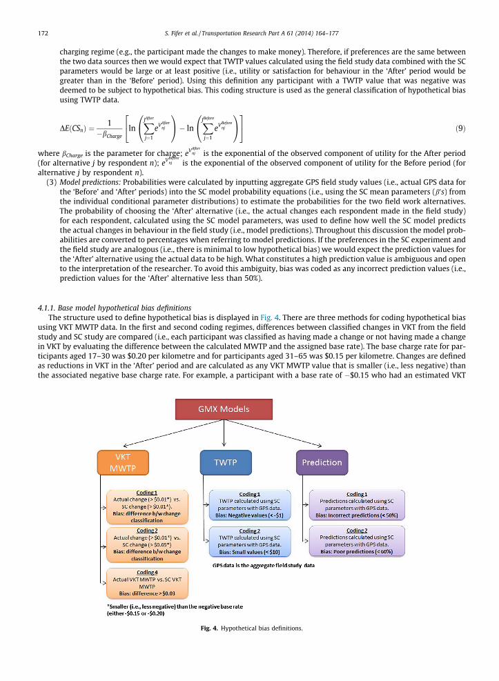
4.1.1. Base model hypothetical bias definitionsThe structure used to define hypothetical bias is displayed in Fig. 4. There are three methods for coding hypothetical bias

using VKT MWTP data. In the first and second coding regimes, differences between classified changes in VKT from the fieldstudy and SC study are compared (i.e., each participant was classified as having made a change or not having made a changein VKT by evaluating the difference between the calculated MWTP and the assigned base rate). The base charge rate for par-ticipants aged 17–30 was $0.20 per kilometre and for participants aged 31–65 was $0.15 per kilometre. Changes are definedas reductions in VKT in the ‘After’ period and are calculated as any VKT MWTP value that is smaller (i.e., less negative) thanthe associated negative base charge rate. For example, a participant with a base rate of �$0.15 who had an estimated VKT

Fig. 4. Hypothetical bias definitions.

S. Fifer et al. / Transportation Research Part A 61 (2014) 164–177 173

MWTP of �$0.10 would be classified as having made a change. Alternatively if the same participant had a VKT MWTP of�$0.25 they would be classified as having made no change. In the SC models there were few respondents with VKT MWTPvalues below the negative base rate (i.e., between �$0.15 or �$0.20 and $0.00). Therefore any SC VKT MWTP that was smal-ler (i.e., less negative) than the negative base rate by more than $0.01 was deemed a change. This same classification wasused for the actual VKT MWTP change classification in coding regime 1. However, in coding regime 2, a change was definedas a VKT MWTP value that was more than $0.05 smaller (i.e., less negative) than the negative base rate. This secondary clas-sification was used to reduce the possibility of incorrect coding because of random fluctuations in behaviour by classifyingonly large changes as relevant. The last coding regime (coding regime 4) directly compared differences between the actualVKT MWTP truncated values and SC VKT MWTP truncated values. In coding regime 4, hypothetical bias was classified as agreater than $0.03 difference between the values.

Two coding structures were used to define hypothetical bias using TWTP data. In coding regime 1, any participant with anegative TWTP value was classified as biased. In addition, a second coding regime was also applied which classified hypo-thetical bias as not only participants with negative TWTP values but also participants with small TWTP values (i.e., <$10).Similar to TWTP bias classifications, two coding structures were used to define hypothetical bias using model prediction val-ues. In the first coding regime, incorrect predictions (i.e., prediction probabilities of less than 50% for the ‘After’ alternative)were coded as affected by hypothetical bias. The second coding regime also included poor predictions, coding any predictionvalues less that 60% as biased.

4.1.2. VKT MWTP hypothetical biasThe total percentage of participants affected by hypothetical bias using the different coding regimes and the direction of

the bias is displayed graphically in Fig. 5. In total the percentage of biased participants is consistent using coding regimes 1and 4 and generally lower using coding regime 2. Regardless of which coding regime is used as the definitive measure, hypo-thetical bias is an issue for a substantial number of participants in this study. The direction of the bias distinguishes whetherthe difference is a result of an observed change in the RP field study and no change in the SC survey or alternatively an ob-served change in the SC survey and no change in the RP field study.

4.1.3. TWTP and model prediction hypothetical biasTWTP hypothetical bias classifications and bias classifications using model prediction values are displayed in Fig. 6. Two

different coding regimes are used to classify hypothetical bias for each measurement (coding regimes 1 and 2). The bias clas-sifications generated using TWTP and model predictions are very similar within each coding regime. On average, hypothet-ical bias percentages calculated using TWTP and model prediction measures are smaller than VKT MWTP hypothetical biaspercentages. Despite this difference, a significant proportion of participants are still considered biased using the TWTP andmodel prediction bias classifications.

4.2. Sources of hypothetical bias

In other studies investigating hypothetical bias, the prevalence of bias is determined by examining aggregate differencesin model outcomes using SP and RP data sources (e.g., generally MWTP and/or TWTP differences). Studying hypothetical biasin this way allows for only a top-line view with limited extension to investigate other influences on hypothetical bias. Morespecifically, aggregate analysis does not allow the researcher to report on the prevalence of hypothetical bias (i.e., how manyparticipants are affected by hypothetical bias) or give any insight into why hypothetical bias occurs (i.e., correlates of hypo-thetical bias). More detailed analysis of individual participants is required to further understand the nature of hypotheticalbias. In this research every individual has been classified into a hypothetical bias category (i.e., biased or not biased) allowingextensive analysis.

Rather than simply splitting the raw data counts by every other variable, a model was used to measure the relationshipsbetween the hypothetical bias measures and other important variables. The use of such a model allowed the relationships to

Fig. 5. VKT MWTP hypothetical bias.

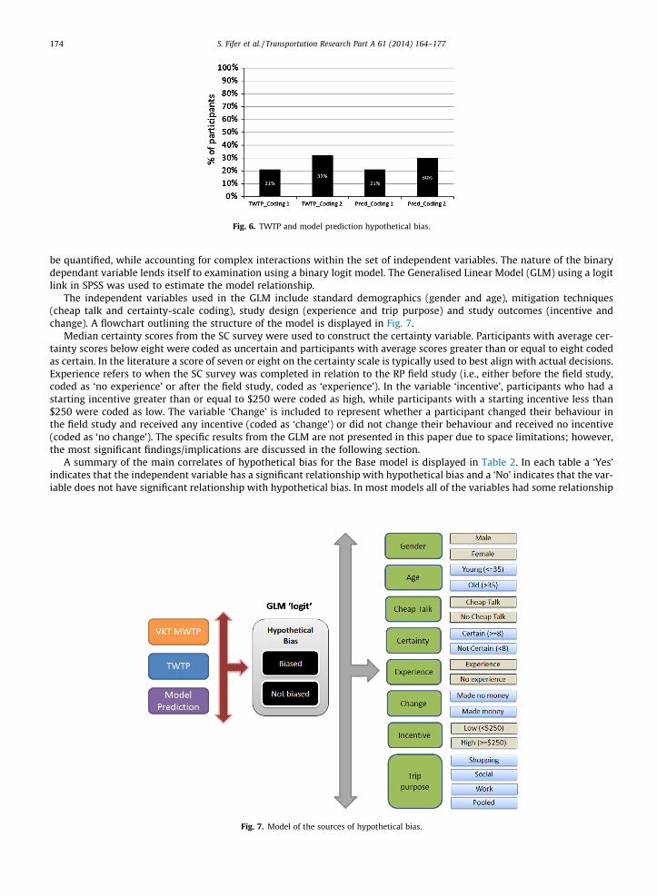
Fig. 6. TWTP and model prediction hypothetical bias.

174 S. Fifer et al. / Transportation Research Part A 61 (2014) 164–177

be quantified, while accounting for complex interactions within the set of independent variables. The nature of the binarydependant variable lends itself to examination using a binary logit model. The Generalised Linear Model (GLM) using a logitlink in SPSS was used to estimate the model relationship.

The independent variables used in the GLM include standard demographics (gender and age), mitigation techniques(cheap talk and certainty-scale coding), study design (experience and trip purpose) and study outcomes (incentive andchange). A flowchart outlining the structure of the model is displayed in Fig. 7.

Median certainty scores from the SC survey were used to construct the certainty variable. Participants with average cer-tainty scores below eight were coded as uncertain and participants with average scores greater than or equal to eight codedas certain. In the literature a score of seven or eight on the certainty scale is typically used to best align with actual decisions.Experience refers to when the SC survey was completed in relation to the RP field study (i.e., either before the field study,coded as ‘no experience’ or after the field study, coded as ‘experience’). In the variable ‘incentive’, participants who had astarting incentive greater than or equal to $250 were coded as high, while participants with a starting incentive less than$250 were coded as low. The variable ‘Change’ is included to represent whether a participant changed their behaviour inthe field study and received any incentive (coded as ‘change’) or did not change their behaviour and received no incentive(coded as ‘no change’). The specific results from the GLM are not presented in this paper due to space limitations; however,the most significant findings/implications are discussed in the following section.

A summary of the main correlates of hypothetical bias for the Base model is displayed in Table 2. In each table a ‘Yes’indicates that the independent variable has a significant relationship with hypothetical bias and a ‘No’ indicates that the var-iable does not have significant relationship with hypothetical bias. In most models all of the variables had some relationship

Fig. 7. Model of the sources of hypothetical bias.

Table 2Summary of GLM findings (base GMX model).

Measurement MWTP TWTP Model predictions

Coding regime 1 2 4 1 2 1 2

Gender No Yes (I) Yes (I) Yes (I) Yes (I) Yes (I) Yes (IM)Age Yes (IM) Yes (I) Yes (I) Yes (I) Yes (IM) Yes (I) Yes (IM)Cheap talk Yes (IM) Yes (I) Yes (I) Yes (I) Yes (I) Yes (I) Yes (I)Certainty Yes (I) Yes (I) Yes (IM) Yes (IM) Yes (IM) Yes (IM) Yes (IM)Experience Yes (IM) Yes (I) Yes (I) Yes (I) Yes (I) Yes (I) Yes (I)Model Yes (IM) Yes (I) Yes (I) N/A N/A N/A N/AChange Yes (I) No Yes (IM) Yes (I) No Yes (I) Yes (IM)Incentive Yes (I) Yes (I) Yes (IM) Yes (I) Yes (I) Yes (I) Yes (I)Trip purpose Yes (I) Yes (I) Yes (IM) Yes (IM) Yes (IM) Yes (IM) Yes (IM)

(I) Included in model as an interaction with other variables, (M) Included in model as a main effect, (IM) Included in model as a main and interaction effect.

S. Fifer et al. / Transportation Research Part A 61 (2014) 164–177 175

with hypothetical bias (i.e., either through an interaction with other variables or as a main effect). The variables with thelargest effects in each model are highlighted.8 The impact of cheap talk is constant across all measures (MWTP, TWTP andmodel predictions) and coding structures. However, the influence of certainty is only evident in TWTP and model predictionmeasures. Trip purpose also has a significant relationship with hypothetical bias. Further details about the modelling of thesources of hypothetical bias can be found in previous research conducted by the authors (Fifer, 2011).

5. Discussions and conclusions

5.1. Prevalence of hypothetical bias

This research supports the existence of hypothetical bias in SC methods irrespective of the model outcomes used to mea-sure the bias, the rules used to define the bias and the mitigation techniques applied to reduce the bias.

Different coding rules for hypothetical bias are applied for each model outcome to test for differences between the SC andRP data sources. Multiple rule definitions are used to represent the lower and upper boundaries of bias. Differences in hypo-thetical bias classifications using the multiple coding regimes represent the sensitivity of the model outcome to hypotheticalbias calculations. In all measurements, even if the most basic coding regime is applied, at least one in five participants arestill affected by hypothetical bias.

Hypothetical bias classifications using TWTP and model predictions were very similar. Although still correlated, MWTPbias classifications did not significantly overlap with TWTP and prediction classifications of bias. Differences between theseresults are to be expected because MWTP calculations do not include the influence of other attributes, including night-timedriving, speeding and travel time increases in this study. Variation in measured bias between the different model outcomesis consistent with other research in the literature where MWTP and TWTP have been compared (Alfnes et al., 2006; Lusk andSchroeder, 2004). These findings demonstrate the importance of the choice of model outcome when evaluating hypotheticalbias.

5.2. Effectiveness of cheap talk as a mitigation method

The effectiveness of cheap talk as a tool to mitigate hypothetical bias varies considerably in the literature. This variation ispartially explained by differences in the type and length of the cheap talk scripts and importantly the context of the SCexperiment. In this research, cheap talk appears to have some influence on hypothetical bias but more so as an interactionwith experience and certainty than as a direct effect.

The inclusion of a cheap talk script emphasises the impact of certainty on hypothetical bias. Whilst not always statisti-cally significant, if after viewing a cheap talk script, respondents are certain of their responses, in almost all cases hypothet-ical bias is lower. These findings imply that participants use the certainty scale differently when shown a cheap talk scriptthan when they are not shown a cheap talk script. In general, therefore, if participants are certain about their survey re-sponses after viewing a cheap talk script, then we can be more confident that their responses will more closely align withtheir actual behaviour. The converse is also true: if participants are not certain about their survey responses after beingshown a cheap talk script then they are more likely to be confused about their decisions and display inconsistences betweentheir survey responses and actual behaviour.

In measuring hypothetical bias, participants with experience are less sensitive to the inclusion of a cheap talk script thanparticipants without experience. This may be because participants with experience are already aware of and familiar withthe decision context and further reminders about possible bias and the importance of their answers through a cheap talk

8 The top 3–4 variables are highlighted in each table. These variables were selected by evaluating the number of times each independent variable featured inthe model (both main and interaction effects) and the significance of these relationships (evaluated using the Wald chi-square statistic and p-values).

176 S. Fifer et al. / Transportation Research Part A 61 (2014) 164–177

script is redundant. This finding is supported by previous research investigating hypothetical bias in CV (Champ et al., 2009).Considered in isolation, this relationship suggests that the use of a cheap talk script is more relevant for studies in whichparticipants have no experience with the decision scenario.

5.3. Effectiveness of certainty scales as a mitigation method

Participant uncertainty is clearly associated with hypothetical bias. It is intuitive to reason that the more certain partic-ipants are about their responses in the SC survey, then the less likely they are to display inconsistencies between these re-sponses and their behaviour in the field study. This influence is apparent as a direct effect and as an interaction effect withother variables in the modelling of the correlates of hypothetical bias. The influence of certainty on hypothetical bias is par-ticularly pronounced for participants with experience and also for participants who are shown a cheap talk script. These re-sults are to be expected because participants with experience are more familiar with the decision scenario and are alreadylikely to have developed some preconceived judgements about the decision scenario. This may lead them to take the choicetask more seriously and make better-informed decisions because they understand how participating in this scheme couldaffect their actual life. Likewise, participants who are shown a cheap talk script are encouraged to take the task more seri-ously and answer as if they were participating in a real scenario. A survey response with higher certainty from participants ineither of these two groups is more likely to be consistent with behaviour in the field study. It is highly recommended thatresearchers and practitioners include a certainty scale in future SC studies to test for these effects.

5.4. Conclusions

This research demonstrates that hypothetical bias is a significant issue in SC surveys. A review of the literature suggeststhat the size and direction of the bias is sensitive to study design and context. In this study, a number of methods are used todefine hypothetical bias to rigorously examine the overall impact. Given the lack of consensus in the literature surroundingthe size and direction of the hypothetical bias, the focus of this research is not on the magnitude of hypothetical bias butrather on its prevalence. Regardless of the particular methods used to assess hypothetical bias, the results indicate that hypo-thetical bias affects at least one in every five participants but up to every second participant. The extent to which the specificresults from this research can be generalised to other SC studies is not clear. However, the results support the theory that SCstudies are inherently prone to hypothetical bias and that mitigation methods can aid in reducing this bias in certaincircumstances.

The practical implications of these findings provide a cautionary warning to researchers and practitioners in this fieldwho use the results from SC models to aid in making important market decisions. Outcomes from this research will hopefullynot detract from the use of SC methods but rather encourage researchers to be aware that a certain level of bias will likely bepresent in SC surveys and they should therefore take the necessary precautions to limit the extent of this bias. These pre-cautions include the use of cheap talk scripts and certainty scales as well as the careful monitoring of sample characteristics(e.g., experience and demographics).

Appendix A. Supplementary material

Supplementary data associated with this article can be found, in the online version, at http://dx.doi.org/10.1016/j.tra.2013.12.010.

References

Aadland, D., Caplan, A.J., 2003. Willingness to pay for curbside recycling with detection and mitigation of hypothetical bias. Am. J. Agric. Econ. 85, 492–502.Alfnes, F., Guttormsen, A., Steine, G., Kolstad, K., 2006. Consumers’ willingness to pay for the color of Salmon: a choice experiment with real economic

incentives. Am. J. Agric. Econ. 88, 1050–1061.Ben-Akiva, M., Morikawa, T., 1990. Estimation of switching models from revealed preferences and stated intentions. Transport. Res. Part A: Gen. 24, 485–

495.Blumenschein, K., Blomquist, G., Johannesson, M., Horn, N., Freeman, P., 2008. Eliciting willingness to pay without bias: evidence from a field experiment.

Econ. J. 118, 114–137.Bradley, M.A., Daly, A.J., 1997. Estimation of Logit Choice Models using Mixed Stated Preference and Revealed Preference Information. Elsevier, Oxford.Brownstone, D., Small, K.A., 2005. Valuing time and reliability: assessing the evidence from road pricing demonstrations. Transport. Res. Part A: Pol. Pract.

39, 279–293.Carlsson, F., Frykblom, P., Lagerkvist, C.-J., 2005. Using cheap-talk as a test of validity in choice experiments. Econ. Lett. 89, 147–152.Carson, R., Groves, T., 2007. Incentive and informational properties of preference questions. Environ. Resour. Econ. 37, 181–210.Champ, P.A., Bishop, R.C., Brown, T.C., McCollum, D.W., 1997. Using donation mechanisms to value nonuse benefits from public goods. J. Environ. Econ.

Manage. 33, 151–162.Champ, P., Moore, R., Bishop, R., 2009. A comparison of approaches to mitigate hypothetical bias. Agric. Resour. Econ. Rev. 38, 166.Cummings, R., Taylor, L., 1999. Unbiased value estimates for environmental goods: a cheap talk design for the contingent valuation method. Am. Econ. Rev.

89, 649–665.Dussán, D.C., Ullrich, H., 2010. Consumer Welfare and Unobserved Heterogeneity in Discrete Choice Models: The Value of Alpine Road Tunnels. ZEW –

Centre for European Economic Research Discussion Paper No. 10-095.Fiebig, D.G., Keane, M.P., Louviere, J., Wasi, N., 2010. The generalized multinomial logit model: accounting for scale and coefficient heterogeneity. Market.

Sci. 29, 393–421.Fifer, S., 2011. Hypothetical Bias in Stated Preference Experiments: Is it a Problem? And if So, How Do We Deal With It? The University of Sydney.

S. Fifer et al. / Transportation Research Part A 61 (2014) 164–177 177

Fifer, S., Greaves, S.P., Rose, J.M., Elisson, R., 2011. A combined GPS/stated choice experiment to estimate values of crash-risk reduction. J. Choice Model. 4,44–61.

Greaves, S.P., Fifer, S., 2010. Development of a kilometre-based charging regime to encourage safer driving practices. Transport. Res. Rec.: J. Transport. Res.Board 2182, 88–96 (Research Board of the National Academies, Washington, DC).

Greaves, S.P., Fifer, S., Ellison, R., Germanos, G., 2010a. Development of a global positioning system web-based prompted recall solution for longitudinaltravel surveys. Transport. Res. Rec.: J. Transport. Res. Board 2183, 69–77 (Transportation Research Board of the National Academies, Washington, DC).

Greaves, S.P., Fifer, S., Ellison, R., Familar, R., 2010b. Development and implementation of a GPS/internet-based design for longitudinal before-and-aftertravel behaviour studies. In: 12th World Conference on Transport Research WCTR, Lisbon, Portugal.

Greene, W., Hensher, D., 2010. Does scale heterogeneity across individuals matter? An empirical assessment of alternative logit models. Transportation 37,413–428.

Harrison, G., 2007. Making choice studies incentive compatible. In: Kanninen, B. (Ed.), Valuing Environmental Amenities Using Stated Choice Studies.Springer, The Netherlands, pp. 67–110.

Harrison, G.W., Rutström, E.E., 2008. Experimental evidence on the existence of hypothetical bias in value elicitation methods. In: Charles, R.P., Vernon, L.S.(Eds.), Handbook of Experimental Economics Results. Elsevier, pp. 752–767 (Chapter 81).

Hensher, D.A., 2010. Hypothetical bias, choice experiments and willingness to pay. Transport. Res. Part B: Methodol. 44, 735–752.Hensher, D.A., Rose, J.M., Bliemer, M., 2010. Course Notes. Discrete Choice Analysis Course, Sydney, Australia.Herriges, J., Kling, C., Liu, C.-C., Tobias, J., 2010. What are the consequences of consequentiality? J. Environ. Econ. Manage. 59, 67–81.Hess, S., Rose, J.M., 2010. Random scale heterogeneity in discrete choice models. In: 89th Annual Meeting of the Transportation Research Board TRB 2010,

Washington, DC, United States.Hess, S., Rose, J.M., 2012. Can scale and coefficient heterogeneity be separated in random coefficients models? Transportation 39, 1225–1239.Isacsson, G., 2007. The Trade off between Time and Money: Is there a Difference Between Real and Hypothetical Choices? Swedish National Road and

Transport Research Institute.Johannesson, M., 1999. Calibrating hypothetical willingness to pay responses. J. Risk Uncertain. 18, 21–32.Ladenburg, J., Olsen, S.B., 2010. Augmenting Short Cheap Talk Scripts with a Repeated Opt-Out Reminder in Choice Experiment surveys. University of

Copenhagen, Institute of Food and Resource Economics FOI Working Paper 2010/9.Li, C.-Z., Mattsson, L., 1995. Discrete choice under preference uncertainty: an improved structural model for contingent valuation. J. Environ. Econ. Manage.

28, 256–269.List, J., 2001. Do explicit warnings eliminate the hypothetical bias in elicitation procedures? Evidence from field auctions for sportscards. Am. Econ. Rev. 91,

1498–1507.List, J., Gallet, C., 2001. What experimental protocol influence disparities between actual and hypothetical stated values? Environ. Resour. Econ. 20, 241–

254.Little, J., Berrens, R., 2004. Explaining disparities between actual and hypothetical stated values: further investigation using meta-analysis. Econ. Bull. 3, 1–

13.Louviere, J.J., Hensher, D.A., Swait, J.D., 2000. Stated Choice Methods: Analysis and Applications/Jordan J. Louviere, David A. Hensher, Joffre Swait, with a

Contribution by Wiktor Adamowicz. Cambridge, UK; New York, NY, US.Lusk, J., Schroeder, T., 2004. Are choice experiments incentive compatible? A test with quality differentiated beef steaks. Am. J. Agric. Econ. 86, 467–482.McFadden, D., 1974. Conditional logit analysis of qualitative choice behaviour. In: Zarembka, P. (Ed.), Frontiers of Econometrics. Academic Press, New York,

pp. 105–142.Moore, R., Bishop, R.C., Provencher, B., Champ, P.A., 2010. Accounting for respondent uncertainty to improve willingness-to-pay estimates. Can. J. Agric.

Econ./Rev. can. d’agroecon. 58, 381–401.Morrison, M., Brown, T., 2009. Testing the effectiveness of certainty scales, cheap talk, and dissonance-minimization in reducing hypothetical bias in

contingent valuation studies. Environ. Resour. Econ. 44, 307–326.Murphy, J., Allen, P., Stevens, T., Weatherhead, D., 2005. A meta-analysis of hypothetical bias in stated preference valuation. Environ. Resour. Econ. 30, 313–

325.Nielsen, O.A., 2004. Behavioral responses to road pricing schemes: description of the Danish AKTA experiment. J. Intell. Transport. Syst.: Technol. Plan. Oper.

8, 233–251.Norwood, F.B., 2005. Can calibration reconcile stated and observed preferences? J. Agric. Appl. Econ. 37, 111.Ready, R.C., Champ, P.A., Lawton, J.L., 2010. Using respondent uncertainty to mitigate hypothetical bias in a stated choice experiment. Land Econ. 86, 363–

381.Rose, J.M., Bliemer, M.C.J., 2009. Constructing efficient stated choice experimental designs. Transp. Rev. 29, 587–617.Rose, J.M., Bliemer, M.C.J., Hensher, D.A., Collines, A.T., 2008. Designing efficient stated choice experiments in the presence of reference alternatives. Transp.

Res. Part B 42, 395–406.Sugden, R., 2005. Anomalies and stated preference techniques: a framework for a discussion of coping strategies. Environ. Resour. Econ. 32, 1–12.Train, K., 2009. Discrete Choice Methods with Simulation, second ed. Cambridge University Press, Cambridge.Vossler, C.A., Evans, M.F., 2009. Bridging the gap between the field and the lab: environmental goods, policy maker input, and consequentiality. J. Environ.

Econ. Manage. 58, 338–345.