Trade and Investment Among BRICS: Analysis of Impact of Tariff Reduction and Trade Facilitation Based on Dynamic

Global CGE Model Libo Wu, Xiangshuo Yin, Changhe Li, Haoqi Qian, Taoran Chen, Weiqi Tang

Abstract: So far, there are few researches based on GTAP model focusing on the inter-regional trade activities among BRICS countries. Specifically, few studies have paid special attention to tariff exemption or trade facilitation scenario analysis. On the other hand, these topics broadly exist in global, multilateral and bilateral trade agreements and dialogues.

One of the most prominent issues calling for in-depth study is the dynamic changing characteristics of emerging economies’ trade activities. BRICS countries differ greatly with respect to their trade volume, structure, dependence and environment, which lead to diversified sensitivities to tariff and trade facilitation. As the largest export-oriented emerging economy, China is more sensitive to tariffs and trade facilitation due to its large trade volume of manufactured goods and primary goods. Brazil and Russia are traditional resources exporter and thus they are less sensitive to tariffs and trade facilities because of the monopoly power. India is more dependent on service trade and commodity trade market is usually protected. However, since all of the BRICS counties have joined WTO and the global trade context is transforming, we need to involve the political and economic dynamics into global trade model to simulate the economic impacts.

In this paper, we established a dynamic global CGE model to analyze the effects of free trade and trade facilitation in BRICS countries. In the settings of our model, we use adaptive expectation other than pure rational expectation to reflect the situation that BRICS countries are in the midst of transformation. The results show that the dynamic trade changing paths of these countries are quite different from those of developed countries.

When trade facilitation increases, the results of China show that China’s agricultural products will see a huge growth in the future. One reason is that agricultural products are very sensitive to trade facilitation, especially sensitive to factors like custom clearance time. Car trade will also see a huge growth under the scenario that car tariffs are reduced.

1. Introduction In the 1960s, Johansen established a multi-sectoral growth model used to study the

economic growth in Norway, which means the beginning of CGE model. Half a century has past, the CGE model was developed quickly in terms of the depth of theory, structure and application field (He etc.2010). So far, almost all the developed countries and most of the developing countries have established their own CGE model, which is widely applied in the field such as the taxation and tax reform, trade liberalization, market and policy reform, income distribution, energy, natural resources and environmental protection (Zhou and Wang, 2006), among which the GTAP model is one of the favorite global model.

In the context of global trade liberalization and GHG reduction, it is easily found that, there are few researches based on CGE/GTAP model focusing on the inter-regional trade activities among countries or regions, although such international coalition is considered to be a promising and effective strategy for global abatement when coalition members are able to take binding commitments as a whole (Peters and Hertwich,2008). On the other hand, while previous studies

usually grouped nations according to their economic conditions, the regions group work is much more complicated than that associated with the simple coalitions grouped in respect of only economic condition (Chen and Chen, 2011). As a result, we take the BRICS countries as representative of the fast developing as well as kind of strongly politic inter-playing countries. In addition, the United States and European Union including 27 European countries are introduced into our analysis to help make a comparison between the “south” and “north” regions. Because the trade liberalization and facilitation are mixes of both economic and politic factors, and the BRICS countries have just entered into the WTO in the last two decades, these two issues are selected as our research points in this paper by using the Dynamic Global CGE model.

2. Literature Review Although researches on global and regional CGE are getting more active, less attention has

been taken to those regions grouped by both the economic and politic standards such as the BRICS countries within the global CGE framework. Separately speaking, Maldonado et al. (2007) modeled foreign capital flow to Brazil as stemming from an investment decision whose risk depended on the expected rate of loss of foreign reserves. By comparing the response of the two versions of the model by simulating the implementation of the trade agreements with the Americas and with the European Union, they concluded that the inclusion of endogenous foreign capital flow in the model significantly amplifies. One of the latest global CGE research publications came from Lemelin et al. (2013), they present an applied CGE world model with financial assets and endogenous current account, along with the capital and financial account balances. Their financial CGE model involves 14 regions including two main BRICS countries China and India. However, the G7 group is not so appropriate in terms of the developed regions due to its smaller scale compared with the OECD, and is less representative than the USA plus EU. Das (2012) also made the two BIRC countries China and India as the core regions in his global CGE model. His model presented that exogenous technology shock from developed North, vehicled via trade, transmits to developing Souths and induces productivity growth. What’s more, dynamism of Southern Engines of Growth – India and China – caused them to emerge as ‘core’ South. Das’s paper shows kind of inter-relationship implication among the developing countries, while the other BRICS countries’ role still unknown. As BRICS are the leading countries in terms of economy development, it is easy to find out that they are often concerned in some other global CGE research works especially in GTAP model (McDonald at al 2008, Walmsley and Hertel 2000, Elena et al 1999, 2006). Pereira et al (2010) analyze the impacts of the Doha Round on Brazilian, Chinese and Indian agribusiness using GTAP 7, compared with the EU 25 regions and the USA as the developed countries. Their research gave many reasonable implications such as the highest growth rate owned by China and Brazil. While some limitations must be figured that it is kind of static model but not a dynamic one, which is not enough to analyze the scenarios of these fast developing countries. Besides, more researches could be found in some regional CGE model focus on Russia (Orlov and Grethe 2012), India (Ojha et al 2013) and China (He et al 2010, Horridge et al 2008) due to the data quality limitation and specific model structure designing. As reviewed above, it is implied that less global CGE modeling work has been done about the BRICS countries, as well as the GTAP modeling.

Since the BRICS countries are the most sensitive regions both in the economic and politic fields, and most of the international issues such as tariff exemption and trade facilitation are very complicated due to the policy intervention, we put our research focus on the BRICS countries’ inter-action, along with their trading and financial relationship with the advanced regions (e.g. EU and the United States) by a global CGE model. For the most obvious feature of the BRICS

countries is the long-lasting fast economic growth, a dynamic model is necessary and introduced in our model.

Because most of the CGE model has often been used to analyze the trade and energy issues just like what Dixion et al. (2006), Hertel (1994) and Böhringer (2011) have done, a tariff reduction scenario is certainly necessary to be introduced into our global CGE model. In addition, there are more measures taken to improve the trade facilitation by some organizations such as the World Customs Organization’s Data Model and Single Window Projects, the UN/CEFACT’s trade facilitation projects, and the EU Blue Belt Pilot Project. So it is reasonable and necessary to analyze the effects of these trade facilitation because these policies are often implemented regionally (EMSA, 2010), partly and temporarily (Trade Facilitation and Port Community System Committee, 2012). We will further introduce the related tariff reduction and facilitation policies in detail in the following processing part.

3. Data Collection and Processing

3.1 Building Regional SAM Table

The data used in the model were derived from the GTAP 8 database (see Narayanan, Hertel and Terrie, 2012) using a three dimensional Social Accounting Matrix (SAM) method for organising the data. Details of the method used to generate a SAM representation are reported in McDonald and Thierfelder (2004a) while a variety of reduced form representations of the SAM and methods for augmenting the GTAP database are reported in McDonald and Thierfelder (2004b) and McDonald and Sonmez (2004) respectively. Detailed descriptions of the data are provided elsewhere so the discussion here is limited to the general principles.

Trade Structure and Industry Structure

For analysis purposes, taking each region’s current overall economic situation into consideration is pretty important. Figure 1 describes the current trade structure of each region. What we can learn from the figure is that percentage of imported value of each region from listed regions excluding Rest of World is quite large. Although structures of these percentages vary from each other, the absolute level ranges from 48.0% to 76.40%, which means international trades between these regions play an quite important role in the world and also inside these regions.

Taking a closer look into these regions’ trade structure, we also find that each BRICS country does have one or two trade partners, which is consistent with our initial assumptions. To this extent, dividing the whole world into these nine regions is reasonable.

0%

10%

20%

30%

40%

50%

60%

70%

80%

90%

100%

BRA RUS IND CHN ZAF USA EUN ASD ROW

BRA RUS IND CHN ZAF USA EUN ASD ROW

Figure 1: Trade structure of each region

Besides current trade structures, industry structures also affect trade policies significantly. For example, if a country or region has a strong service industry, then without enhancing its manufacturing efficiency, it cannot benefit a lot from introducing export-encouraging policies. Moreover, if a country or region has a strong primary industry with high production efficiency, its agricultural product exports will present high sensitivity to the level of trade facilitations. Figure 2 shows different industry structures in each region.

Figure 2: Economic structure of each region Global Social Accounting Matrix

The Global SAM can be conceived of as a series of single region SAMs that are linked through the trade accounts. In the context of the GTAP database, it is particularly easy to construct a SAM table for each country. However, the only way to directly link these regions together is through international commodity trade transactions, although there are some indirect

links through the demand and supply of trade and transport services. Specifically the value of exports, valued free on board (fob) from source x to destination y must be exactly equal to the value of imports valued fob to destination y from source x, and since this holds for all commodity trade transactions the sum of the differences in the values of imports and exports by each region must equal zero.

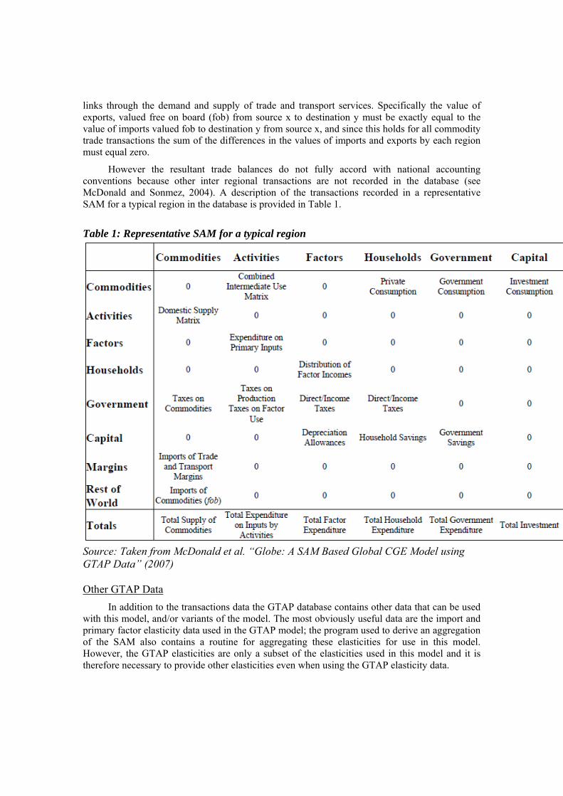
However the resultant trade balances do not fully accord with national accounting conventions because other inter regional transactions are not recorded in the database (see McDonald and Sonmez, 2004). A description of the transactions recorded in a representative SAM for a typical region in the database is provided in Table 1.

Table 1: Representative SAM for a typical region

Source: Taken from McDonald et al. “Globe: A SAM Based Global CGE Model using GTAP Data” (2007) Other GTAP Data

In addition to the transactions data the GTAP database contains other data that can be used with this model, and/or variants of the model. The most obviously useful data are the import and primary factor elasticity data used in the GTAP model; the program used to derive an aggregation of the SAM also contains a routine for aggregating these elasticities for use in this model. However, the GTAP elasticities are only a subset of the elasticities used in this model and it is therefore necessary to provide other elasticities even when using the GTAP elasticity data.

Global SAM Table Adjustments

Besides the basic GTAP data we mentioned above, some additional adjustments need to be applied to finish building global SAM table. When we are aggregating individual regional SAM table of different regions such as EU, Asian developed countries and Rest of world, some part of their original international trade activities should be considered as domestic activities, thus reducing the total amount of import and export value which are obtained through simply addition. For example, in practice, it will be strange that one region export its domestic commodities to itself and classify them as international transactions.

However, the aggregation software provided by GTAP does not take this situation into consideration. After aggregating the data, we see that the self-export data of EU, ASD and ROW do not equal to zero. To avoid this, we subtract these values from export and add them back to domestic input. Consequently, we also subtracted associated export taxes, import taxes and transportation services, and added them back to domestic sales taxes and domestic transportation input.

3.2 Empirical Results of Free Trade and Trade Facilitation

This part presents the policy scenario of both trade facilitation and tariff reduction based on experiences from developed countries and world trade organizations. Firstly we reviews preview researches on both issues based on CGE method, and then we turn to BRICS and design 4 possible policy scenarios.

Trade facilitation

Trade facilitation most often implies improving efficiency in administration and procedures, along with improving logistics at ports and customs. A broader definition includes streamlining regulatory environments, deepening harmonization of standards, and conforming to international regulations (Woo and Wilson 2000). Emphasizing broader concepts of trade facilitation is particularly important given the increasing volume of global trade, the time sensitivity of intermediate goods trade (Hummels 2001), reductions in protective tariff rates, and increased availability of modern technology that can improve the management of cross-border trade.

However, several challenges are apparent in empirical research on trade facilitation: defining and measuring trade facilitation, choosing a modeling methodology to estimate the importance of trade facilitation for trade flows, and designing a scenario to estimate the effect of improved trade facilitation on trade flows.

Several recent studies use CGE models to quantify the benefits of improved trade facilitation. In CGE models an improvement in trade facilitation can be modeled equivalently as a reduction in the costs of international trade or as an improvement in the productivity of the international transport sector.

It is analyzed by the APEC (1999) using CGE that the shock reduction in trade costs from trade facilitation efforts differs among members of the group, with one percent reduction in import prices for the industrial countries and the newly industrializing economies and two percent for the others. It is estimated that APEC merchandise exports would increase by 3.3 percent from the trade facilitation effort to reduce costs. In comparison, the model estimates a long-run increasing of 7.9 percent in APEC merchandise exports from completing Uruguay Round commitments. Hertel et al. (2001) used CGE model to quantify the impact on trade of harmonizing standards for e-business and automating customs procedures between Japan and

Singapore. They found that these reforms will increase trade flows between these countries as well as with the rest of the world.

Much research has been done to assess the effects of trade barriers on patterns of international trade. The method developed for this purpose permit the formal presentation of how formal trade barriers might impact trade volumes. Among them, relatively less study has been conducted on informal trade barriers impact trade volumes, due to the measuring difficulty. As a consequence, researchers rely primarily on indirect methods: posting a model of bilateral trade flows and correlating flows with proxy variables meant to represent trade barriers.

Fox et al. (2003) measured the micro economic impact of the inefficiencies of border crossing in the U.S. - Mexican border on shippers and the institutional factors and vested interests that permit the inefficiencies to appear and last for extended period of time. They defined inefficiencies as money paid by shippers for charges for non-essential border crossing services and the times involved in each step of the border crossing operation. Haralambides et al. (2002) simulated the movements of a track transporting shipments from Chicago to Monterrey. Engels et al. (2001) mentioned the informal trade barriers that exist as one possible explanation for the relatively large border effect for pairs without identifying them.

For the numerical estimation, a study commissioned by the European Commission states that the costs of complying with these unnecessary and mistaken requirements amount to account for 3.5-7 percent of the value of the goods (OECD, 2002). For specific transportation such as shipping, it is argued that each day saved in shipping time would be worth about 0.5 percent of the value of the goods (Hummels, 2001).

Another Hummels’ (2011) research indicate that each day saved in shipping time is worth 0.8 percent ad valorem for manufactured goods. Applying this estimate, and considering that manufactures have to wait from 2 to 5 days to cross the border southbound, this is equivalent to a tariff from 1.6 percent to 4 percent or more, according to the number of days the cargo has to wait to cross the border. Also he estimates the language effects are a significant trade barrier and that speaking a common language lowers costs by an average of 5 percent. The price premier indicate that importers will pay a 3 to 5 percent premium to trade with partners of a common language and 1 to 3 percent premium to trade with contiguous partners.

According to the Trade Facilitation and Port Community System Committee, the latest facilitation projects mainly come from three organizations, World Customs Organization (WCO), NCEFACT and European Union (EU) as mentioned above, among which two of the most representative projects are the so named Blue Belt Project and the Single Window Project.

The Blue Belt Project started in May 2011, with the aim of exploring new ways to promote and to facilitate Short Sea Shipping in the European Union by reducing the administrative burden for intra-Community trade. According to its content, this on-going Blue Belt Pilot project is kind of regionally (only within the intra-EU area) and partly (just for the short sea shipping transport) implemented trade policy. And this kind of facilitation measure maybe extended to a larger region scale. So it is reasonable to set a scenario to simulate the Blue Belt facilitation project which means that different regions may have different transportation cost via different vehicles.

The Single Window systems are considered to be an effective means to establish improved information sharing between government agencies and businesses involved in cross-border trade. It can be used to eliminate inefficiency and ineffectiveness in business and government procedures and document requirements along the international supply chain, reduce trade transaction costs, as well as improve border control, compliance and security. And some of the benefits from the Single Window Project has been calculated by the UNNexT (2009). Here we just list part of the result which is the basic source of our Single Window facilitation scenario.

Germany: It is estimated that users of Dakosy, an electronic document exchange system for sea-port operations in Hamburg, may save approximately €22.5 million per annum simply by reducing labor costs associated with correcting errors during the preparation and submission of trade and transport documents. This €22.5 million savings is based on the assumption that the average cost to employ a person in Germany is €50,000 annually. On average a user of Dakosy can potentially save 9 person-year by reducing a typical error rate of 50% to virtually zero, assuming that an average of 10 minutes of staff time is required to correct each mistake in the paper-based process. Therefore, on one million B/Ls processed each year in Germany, this reduction in error rework equates to a savings of 450 person-years per year (Adobe, 2006).

Republic of Korea: The total savings for the business community from the use of the TradeHub in the Republic of Korea are estimated to be US$ 1.819 billion. These savings are a result of cheaper e-documents transmission cost, improved productivity from the automation of administrative work, and improved management of trade information and documents (UNNexT, 2009).

Singapore: After introducing Single Window in Singapore, the time to process trade documents was reduced from 4 days to 15 minutes (Neo, King, and Applegate, 1995).

Thailand: Partial implementation of Single Window in Thailand has eliminated redundant processes in the export of ordinary goods and reduced the number of days for export from 24 days in 2006 to 14 days in 2009 (Keretho, 2009).

As a summary, we decide to set the average time cost before and after the trade facilitation policies for the developed countries 4-day to 10minutes from 2007 to 2020, which means 4 days of time cost saving generally. And for the developing countries, the saving time is about 10 days.

Tariff reduction

The Uruguay Round in 1999 reached an agreement aiming at discouraging trade-distorting domestic support, non-tariff barriers, and reducing direct export subsidies, among other things. Doha Round followed this pattern, regarding the ease of agricultural commodity access into the world market including the reduction of agricultural production and export subsidies, and the reduction of tariffs on imported agricultural goods.

BRICS members have a special interests in the results reached at the Doha Round. Brazil, China and India have accomplished substantial growth in the international trade market and agricultural trades are concentrated in the export of soy, coffee, meats, sugar and cotton. Much room is provided to grow in terms of agricultural product exports.

Some researches shed lights on the potential reduction of agribusiness product trade barriers at the Doha Round. Such studies have demonstrated high potential gains to developing countries by the elimination of trade barriers.

Conforti et al. (2004) used the GTAP model to investigate the impacts of alternative scenarios of trade liberalization in agricultural markets under the Doha Round. The results show that both developed and developing countries could gain welfare.

Polaski (2006) also used the GTAP model to show that with the achievements of the Doha Round, China would gain around 0.8 to 1.2% of the GDP under certain scenarios.

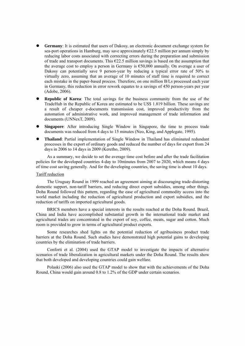
4. Model Structure We established a dynamic global CGE model whose benchmark scenario is calibrated

according to the GTAP 8 Data Base (Reference year: 2007). The model included 9 regions (BRICS, USA, EU, Asian developed countries and Rest of world), and each region has 57 production sectors, one representative household and one regional government. Labor (L) including skilled and unskilled labor, capital (K), land (D) and natural resource (R) are four factors of production.

Figure 3: A multiregional open economy without government intervention.

4.1 Production & demand module

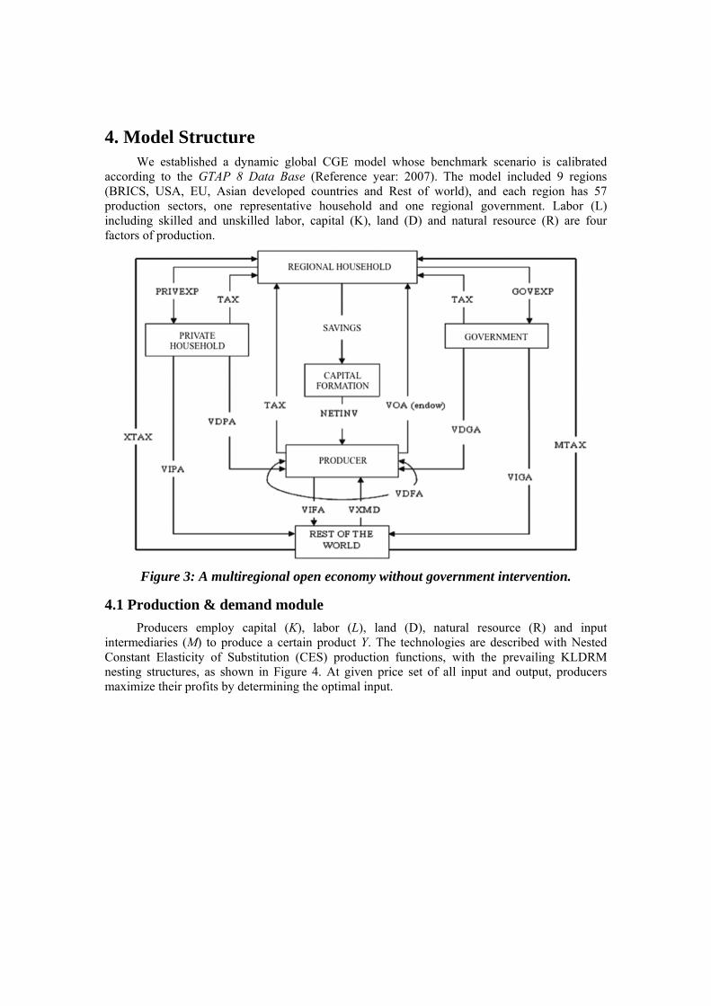
Producers employ capital (K), labor (L), land (D), natural resource (R) and input intermediaries (M) to produce a certain product Y. The technologies are described with Nested Constant Elasticity of Substitution (CES) production functions, with the prevailing KLDRM nesting structures, as shown in Figure 4. At given price set of all input and output, producers maximize their profits by determining the optimal input.

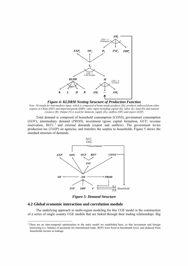
Figure 4: KLDRM Nesting Structure of Production Function

Note: M stands for intermediary input, which is composed of home-made products (Dj), products inflowed from other regions in China (INF) and imported goods (IMP); other input including capital (K), labor (L), land (D) and natural

resource (R). Output (Y) is used for domestic supply (Dj), outflow (OF) and export (EXP)

Total demand is composed of household consumption (CONS), government consumption (GOV), intermediary demand (PROD), investment (gross capital formation, GCF; revenue reservation, REV) 1 and external demands (export and outflow). The government levies production tax (TAXP) on agencies, and transfers the surplus to households. Figure 5 shows the standard structure of demands.

Figure 5: Demand Structure

4.2 Global economic interaction and correlation module

The underlying approach to multi-region modeling for this CGE model is the construction of a series of single country CGE models that are linked through their trading relationships. Big

1 There are no inter-temporal optimization in the static model we established here, so that investment and foreign

borrowing (i.e. balance of payments for international trade, BOP) were fixed at benchmark level, and deduced from households income as leakage.

Economy Assumption is followed in modeling international trade of each region, i.e. international market demand/supply will be affected by endogenous international market prices, and vice versa.

GTAP database has already collected international bilateral trade data, i.e. we can get trade value, both fob and cif price, of a specific commodity from one region to another. The difference between fob and cif price of each commodity is called transportation service cost or transportation margin (see eq.1), we here do not follow the method proposed by McDonald, Thierfelder and Robinson (2007) which treats these transportation using a international sector called GLOBE. In contrast, we treat these transportation services as domestic economic activities, which are produced by domestic capital investment and input into importing activities. This is a key assumption in our model.

IMPi i1MARGINi i2 ir INFLir (1 IMrateir )

r 1

-1

INFL means import goods excluding import tariffs, IMrate means import tariff rates, MARGIN means transportation service costs.

When building a global CGE model, there are usually two ways to treat international trade. In simplified multi-regional CGE models, an extra region (ROW) is introduced to serve as a transit for all the trade flows. It’s a compromise since data for inter-regional trade are not readily available, but the simplification ignored the impact of difference in trade costs and preferences across regions, which could be crucial for determining trade flows (see Figure 6). In order to model global trade flow more precisely, we need to obtain service and transportation costs associated with import goods. GTAP 8 database does include transportation services costs, which are also called margins mentioned above.

Figure 6: Comparison between “Multi-Regional” and “Inter-Regional” Structures

The Armington assumption is used for trade. Domestic output is distributed between the domestic market and exports according to a three-stage Constant Elasticity of Transformation (CET) function. In the first stage a domestic producer allocates output to the domestic or export market according to the relative prices for the commodity on the domestic market and the composite export commodity, where the composite export commodity is a CET aggregate of the exports to groups of regions that have common characteristics, and these second level composite commodities are themselves aggregates of the exports to different regions – the distribution of the exports between regions being determined by the relative export prices to those regions and the presumed substitutability of the commodities based on characteristics of the commodities and the

regions. Consequently domestic producers are responsive to prices in the different markets – the domestic market and all other regions in the model – and adjust their volumes of sales according relative prices. The elasticities of transformation are commodity, region and region group specific. The CET functions across exports can be switched off so that export supplies are determined by import demands, and appropriate parameter specification allows the model to collapse so that it operates in the same way as a model with two-stage transformation functions.

Domestic demand is satisfied by composite commodities that are formed from domestic production sold domestically and composite imports. This process is modeled by a two-stage CES function. At the bottom stage a composite import commodity is a CES aggregate of imports from different regions, where the quantities imported from different regions being responsive to relative prices. The top stage defines composite consumption commodities as CES aggregates of domestic commodities and composite import commodities; the mix being determined by the relative prices. The elasticities of substitution are commodity and region specific. Hence the optimal ratios of imports to domestic commodities and exports to domestic commodities are determined by first order conditions based on relative prices.

ci i2Di i 3 i IMPi

i 1

-1

where ci is the combined consumption of commodities; subscribe r stands for the source region of inflow; ϕ and δ are Armington elasticity of substitution of different nesting layers; and α, θ are cost share parameters.

4.3 Dynamic module of accumulation for heterogeneous capital

One key assumption in our dynamic model is that capital is heterogeneous among different production sectors, which means once newly formed capital is put into production, it becomes specific capital stock and cannot transfer to other sectors in the future. This important characteristic of capital allows us to simulate the economy behavior of BRICS who are experiencing their transitional period.

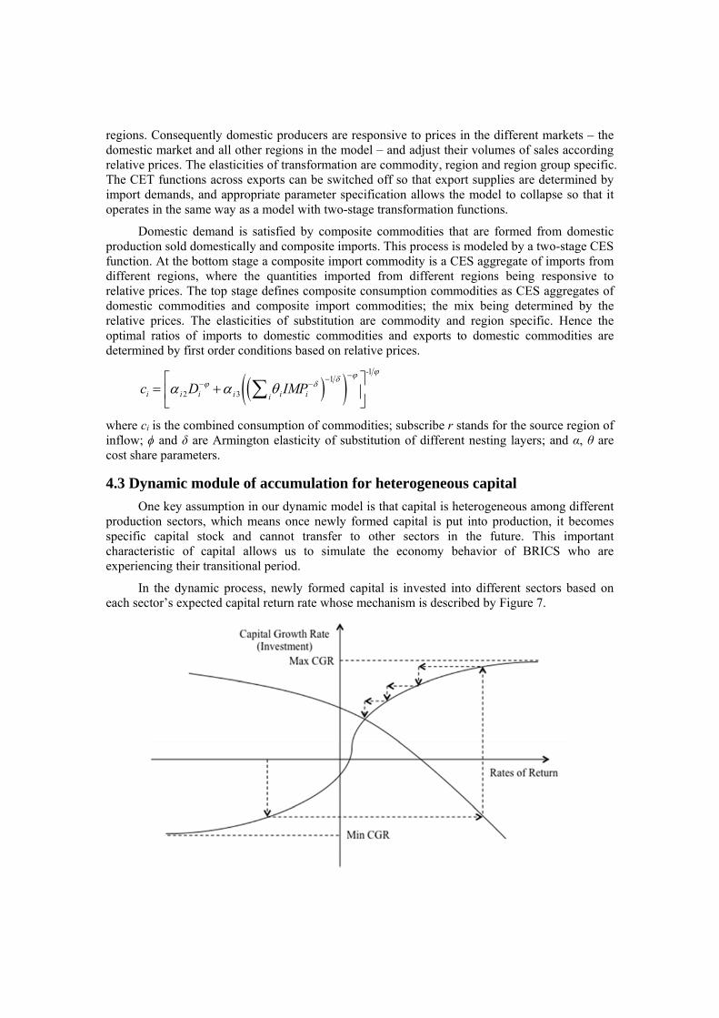
In the dynamic process, newly formed capital is invested into different sectors based on each sector’s expected capital return rate whose mechanism is described by Figure 7.

Figure 7: Dynamic mechanism for capital adjustment

As shown in Figure 7, the relationship between capital growth rate and rates of return comply with a logistic curve. Capital growth rate is bounded by a maximum rate and a minimum rate. When taking depreciation into consideration, the two bound rates are 0.3 and 0, respectively:

1

ei i

ei i

i i c r r

i ii

i i c r r

i i

KR KRe

KR KRKR

KR KRe

KR KR

where KRi is the baseline capital growth rate; KRi and KRi stand for max and min capital

growth rates; ri is the baseline capital return rate of sector i; rie stands for expected capital return

rate of sector i.

5. Policy Scenarios and Simulation Results We present here 4 possible policy scenarios. Simulations of the changes specified in each

of the four scenarios are run and the results from these simulations are analyzed.

Scenario 1: zero tariff

In scenario 1 we assume that each region in our model has free access to export market, which means that no tariff will be existed from the year 2008.

Scenario 2: tariff reduction

We reduce import tariffs to all commodities using the Harbinson approach (see Table 2).The scenario employing the Harbinson approach implements a simple proportional cut, frequently described in policy discussions as a linear cut. Because the tariff reduction schedule and extend often differ among regions, we simply set the reduction schedule is from 2007 to 2015. Then all the tariff keep unchanged.

Table 2: Scenarios for tariff reduction (Harbinson approach) Developed countries Developing countries

Current tariff level Reduction Current tariff level Reduction 0%-15% 40% 0%-20% 25%

15%-90% 50% 20%-60% 30% >90% 60% 6%-120% 35%

>120% 40%

Source: adapted from Antimiani et al. (2006).

Scenario 3: trade facilitation

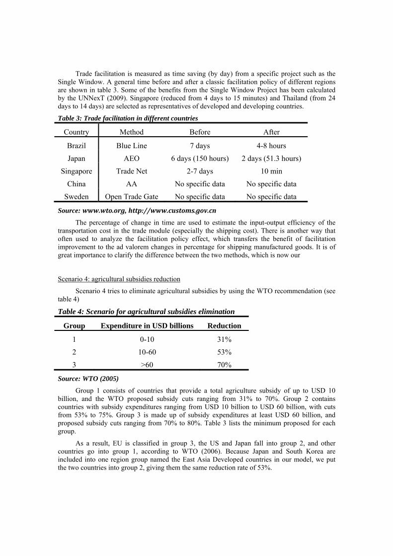
Trade facilitation is measured as time saving (by day) from a specific project such as the Single Window. A general time before and after a classic facilitation policy of different regions are shown in table 3. Some of the benefits from the Single Window Project has been calculated by the UNNexT (2009). Singapore (reduced from 4 days to 15 minutes) and Thailand (from 24 days to 14 days) are selected as representatives of developed and developing countries.

Table 3: Trade facilitation in different countries

Country Method Before After

Brazil Blue Line 7 days 4-8 hours

Japan AEO 6 days (150 hours) 2 days (51.3 hours)

Singapore Trade Net 2-7 days 10 min

China AA No specific data No specific data

Sweden Open Trade Gate No specific data No specific data

Source: www.wto.org, http://www.customs.gov.cn

The percentage of change in time are used to estimate the input-output efficiency of the transportation cost in the trade module (especially the shipping cost). There is another way that often used to analyze the facilitation policy effect, which transfers the benefit of facilitation improvement to the ad valorem changes in percentage for shipping manufactured goods. It is of great importance to clarify the difference between the two methods, which is now our

Scenario 4: agricultural subsidies reduction

Scenario 4 tries to eliminate agricultural subsidies by using the WTO recommendation (see table 4)

Table 4: Scenario for agricultural subsidies elimination

Group Expenditure in USD billions Reduction

1 0-10 31%

2 10-60 53%

3 >60 70%

Source: WTO (2005)

Group 1 consists of countries that provide a total agriculture subsidy of up to USD 10 billion, and the WTO proposed subsidy cuts ranging from 31% to 70%. Group 2 contains countries with subsidy expenditures ranging from USD 10 billion to USD 60 billion, with cuts from 53% to 75%. Group 3 is made up of subsidy expenditures at least USD 60 billion, and proposed subsidy cuts ranging from 70% to 80%. Table 3 lists the minimum proposed for each group.

As a result, EU is classified in group 3, the US and Japan fall into group 2, and other countries go into group 1, according to WTO (2006). Because Japan and South Korea are included into one region group named the East Asia Developed countries in our model, we put the two countries into group 2, giving them the same reduction rate of 53%.

5.1 Baseline Scenario

We first conduct a baseline scenario named S0 without setting any tariff reduction or subsidy elimination from the on-going world trade system. The result is shown in Figure 8. It is realized that the BRICS countries are in the leading role of GDP and welfare increase. Russia and India show a stronger power to climb up in the recent years, while China will lead again around the year 2020 after a short economic recession. In terms of the export growth rate, no big difference has been found among these regions, except for China’s on-going situation. According to the basic view, it is implied that the BRICS countries are still the fastest developing regions in the next decade while their interior structures and inter-relationships are in the process of transition through trade and other forms. What would the economic features changed once specific policies implemented? In the following part, we make a further analysis on the deep impacts of possible policies on the BRICS regions’ output and welfare.

Figures in turn: GDP, welfare and export growth rate

Figure 8: Baseline scenario results of total output, welfare and export

5.2 Simulation results

In addition to the base scenario S0, we have totally conducted four simulation scenarios, denoted as S1 to S4. We have made simulations of the zero tariff, tariff reduction, trade facilitation and agricultural subsidy reduction scenario respectively.

5.2.1 General impacts on trade volume of different scenarios

Before presenting the detail results of the four scenarios, we firstly make a general comparison study about the impacts on the trade export volumes of different scenarios, especially in the five BRICS countries (See figure 9). It can be basically learned from these figures that the zero tariff scenario (S1) cause the biggest long-lasting export increasing from 2008 to 2020, which may thought to be the most potential for all possible policies. India performs the best in S1.

Scenario 2, known as the tariff reduction policy, presents a relatively slower but reasonable export growth route, compared with the zero tariff scenario. The facilitation scenario seems as effective as the tariff red uction measures, given the regions Brazil where S3 are more beneficial than S2 while the others more or less the same. The last scenario seems less sensitive with all the total exports of BRICS a little negative or zero growth. To make a short conclusion, strong tariff reduction policy tools are more efficient than the facilitation measures in terms of the BRICS export promotion, if not, both kinds of policies are available. Meanwhile, the policy of the agricultural subsidy reduction is not so effective. A fully fulfilled policy would be more beneficial.

Figures in turn: China, Brazil, India, Russia and South Africa

Figure 9: Export change rate of BRICS countries in four scenarios

5.2.2 Zero tariff scenario

Figure 10 shows the total GDP increase rate, as well as the welfare change rate for each region within the zero tariff scenario, compared with the baseline result. From the view of total output, it can be learned that all the regions enjoy a long-lasting positive increasing rate from the tariff elimination throughout these simulation years, which is obviously acceptable in common

sense. From the view of the welfare, the figure presents a contrary results for BRICS and the developed countries. All the BRICS countries gain a lot of benefit especially in China, India and Russia. In contrast, the developed regions except some countries in EU and USA suffer a little welfare loss when there is no tariff. This could be explained from the countries’ economic structure. For those fast developing regions which heavily depend on their trade export, no matter the industry intermediate products or the resources export, a sudden tariff elimination will bring a huge export exploration potential, which can keep a very long time and leave the social benefit increase as well.

Figure 10: Total regional GDP increase rate (left) and welfare change rate (right) in S1

5.2.3 Tariff reduction scenario

Similar with the zero tariff scenario (S1), Figure 11 shows the total GDP increase rate and the welfare change rate for each region of the tariff reduction scenario, also compared with the baseline result. Before the tariff reduction target completely achieved in 2015, the Asia developed countries Japan and South Korea grow faster even than China, Russia and India, although these regions are always the top in terms of the aggregate economy growth. China gains more once the tariff reduction target has been finished, along with all the other regions presenting a relatively stable increasing speed during the whole simulation period. Brazil is the only special region that suffers the negative GDP increase. The welfare growth route is quite similar with what we present in scenario S1, which means the developing countries gain while most of the developed loss.

To conclude about S1 and S2 for both of them are tariff related scenarios, it is implied that the tariff reduction or elimination policies are more profitable for the developing countries especially for China, India and Russia in BRICS when we look at their GDP as preventative benchmark and social welfare growth. Although the EU and USA also get bigger GDP value but relatively lower growth rate, their social welfare lost compared with the baseline scenario.

Figure 11: Total regional GDP increase rate (left) and welfare change rate (right) in S2

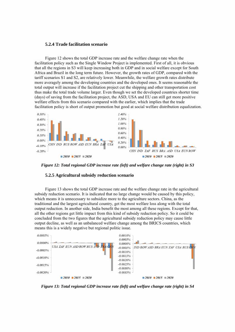
5.2.4 Trade facilitation scenario

Figure 12 shows the total GDP increase rate and the welfare change rate when the facilitation policy such as the Single Window Project is implemented. First of all, it is obvious that all the regions in S3 will keep increasing both in GDP and in social welfare except for South Africa and Brazil in the long term future. However, the growth rates of GDP, compared with the tariff scenarios S1 and S2, are relatively lower. Meanwhile, the welfare growth rates distribute more averagely among the developing countries and the developed ones. It seems reasonable the total output will increase if the facilitation project cut the shipping and other transportation cost thus make the total trade volume larger. Even though we set the developed countries shorter time (days) of saving from the facilitation project, the ASD, USA and EU can still get more positive welfare effects from this scenario compared with the earlier, which implies that the trade facilitation policy is short of output promotion but good at social welfare distribution equalization.

Figure 12: Total regional GDP increase rate (left) and welfare change rate (right) in S3

5.2.5 Agricultural subsidy reduction scenario

Figure 13 shows the total GDP increase rate and the welfare change rate in the agricultural subsidy reduction scenario. It is indicated that no large change would be caused by this policy, which means it is unnecessary to subsidize more to the agriculture sectors. China, as the traditional and the largest agricultural country, get the most welfare loss along with the total output reduction. In another side, India benefit the most among all these regions. Except for that, all the other regions get little impact from this kind of subsidy reduction policy. So it could be concluded from the two figures that the agricultural subsidy reduction policy may cause little output decline, as well as an unbalanced welfare change among the BRICS countries, which means this is a widely negative but regional politic issue.

Figure 13: Total regional GDP increase rate (left) and welfare change rate (right) in S4

5.2.6 Special issue I: Common measures of BRICS countries

This special issue is supposed to make analysis on the effects of the common measures including the above four scenarios only within the BRICS countries. The regional coalitions of BRICS are becoming more important not only because they are the major economic growing powers of the world, but also because they have realized to make some interior economic measures together in order to change the on-going world economic situation and gain strengths. In this special analysis, no changed will be put on S1 to S4 except the implementing regions. So another four scenarios are introduced as BRICS inter-tariff elimination (S5), BRICS inter-tariff reduction (S6), BRICS inter-trade facilitation (S7) and BRICS agriculture subsidy reduction (S8).

The results of effects on GDP growth rate and social welfare changes of different measures are shown in appendix I. And the main scenarios simulation results and possible reasons are explained below.

In S5, Russia, South Africa and China get faster GDP growth rate while Brazil and India get worse compared with the BAU scenario. In terms of welfare, there are two opposite trends in BRICS: China, Russia and India get better, while Brazil and South Africa slow down their growth rate. However, the general growth rates of both GDP and welfare are smaller than the worldwide tariff elimination (S1). A similar story could be told through tariff reduction scenario (S6), with all regions show the same trends but smaller extend to S5.

In the inter-trade facilitation scenario (S7), all the BRICS benefit consistently while all the others suffer loss. China and India are the most beneficiary countries. Comparing with S6, it is indicated that the interior facilitation measures are better than tariff reduction in the GDP and welfare promotion. Moreover, all the BRICS countries could gain from the measure, which means it is easier to implement interior inter-facilitation measures within the BRICS countries than tariff reduction. The effect of S8 looks also invalid just like S4. China, Brazil and India suffer the most.

To look at the exports change rate together about the four BRICS inner measures together. Tariff elimination measure is also the most beneficial policy while its effect in all regions are much smaller than the worldwide elimination (S1). Tariff reduction is better than trade facilitation in promoting exports. And S8 is still ineffective.

5.2.7 Special issue II: exchange rate

Finally, the real exchange rate is analyzed in order to see the effects of different measures on regional real purchasing power. Eight scenarios mentioned above have been compared. It is implied that within the baseline scenario, all regions real exchange rates (regional price/USD) will decrease. China and India decline the most.

Figure 14: Real exchange rate in baseline scenario

Compared with the BAU real exchange rate, the regional prices will increase more under the worldwide measures, bringing less pressures on local appreciation. Among worldwide policies (S1-S4), facilitation causes faster region price increasing. Among interior policies, tariff reduction is more significant. The faster local price raises, the less pressure of appreciation will be given. See related figures in the appendix II.

6. Conclusion and Policy Implication As a conclusion, the BRICS countries develop the fastest under the on-going trade policy

framework in future. From the simulation results, we can see that an increase in BRICS countries’ openness will increase their aggregate economy levels, as well as the social welfare and export, especially for China and Russia. However, united action such as tariff reduction and agricultural subsidy reduction would cause unbalanced growth results, means there actually exists some differences among BRICS countries. Simulation in agricultural subsidies elimination also provides us the information about EU and USA’s strong productivity efficiency in agriculture sectors. Although they have a relatively small portion of primary industry in their whole economy, they can rely on their production efficiency in agriculture sectors to earn significant benefits in whole worlds competition. However, the agricultural subsidies reduction shows the least effect, compared with the trade tariff reduction and facilitation measures.

Trade tariff elimination and reduction policies show the strongest economic promotion function, while the trade facilitation measures are better for the balance of global social welfare distribution. All simulated scenarios, except for the agricultural subsidy reduction, will be beneficial for China and some other fast developing countries. Considering the unbalance among the BRICS and the developed countries’ loss, those trade policies are still not easy to implement. To make a further analysis, issues about the real exchange rate and inter BRICS policies would be raised in our next step.

References André Lemelin, Véronique Robichaud, Bernard Decaluwé, (2013), ‘Endogenous current

account balances in a world CGE model with international financial assets’, Economic Modelling, Vol 32, pp. 146–160.

Anton Orlov, Harald Grethe, (2012), ‘Carbon taxation and market structure: A CGE analysis for Russia’, Energy Policy, Vol 51, pp. 696–707.

APEC Economic Committee. Measuring the Impect of APEC Trade Facilitation on APEC Economies: A CGE Analysis. APEC 2002, Singapore.

Conforti, P., & Salvatici, L. (2004). Agricultural trade liberalization in the Doha Round. Alternative scenarios and strategic interacti ons betwe en developed and developing countries . 7th Annual conference on global economic analysis (pp. 17− 19).

Engel, Ch. and Rogers, J.(December 1996) “How Wide is the Border?” American Economic Review , 86, No 5, pp. 1112-125.

Fox, A. K., Francois, J., & Londono-Kent, P. (2003). Measuring border crossing costs and their impact on trade flows: The United States-Mexican trucking case. In Document presented at the sixth conference on Global Economic Analysis, LaHaye, Pays-Bas.

Gouranga Gopal Das, (2012), ‘Globalization, socio-institutional factors and North–South knowledge diffusion: Role of India and China as Southern growth progenitors’, Technological Forecasting & Social Change, Vol 79, pp. 620–637.

Haralambides, Hercules, and Londoño-Kent, Pilar. “Impediments to Free Trade: The Case of Trucking and NAFTA in the U.S.-Mexican Border”, mimeo, Erasmus University, 2002.

Hertel, T., Hummels, D., Ivanic, M., & Keeney, R. (2007). How confident can we be of CGE-based assessments of Free Trade Agreements?. Economic Modelling, 24(4), 611-635.

Hertel, Thomas, Walmsley, Terrie, and Itakura, Ken (2001) “Dynamic Effects of the “New Age” Free Trade Agreement between Japan and Singapore”, Journal of Economic Integration, pp. 446-484.

Hummels, David. “Time as a Trade Barrier.” Working paper, Purdue University, July 2001.

Mark Horridge, Glyn Wittwer, (2008), ‘SinoTERM, a multi-regional CGE model of China’, China Economic Review, Vol 19, pp. 628–634.

Matheus Wemerson GOMES PEREIRA, Erly Cardoso TEIXEIRA, Sharon RASZAP-SKORBIANSKY, (2010), ‘Impacts of the Doha Round on Brazilian, Chinese and Indian agribusiness’, China Economic Review, Vol 21, pp. 256-271.

McDonald, S., and Thierfelder, K., (2004a). ‘Deriving a Global Social Accounting Matrix from GTAP version 5 Data’, GTAP Technical Paper 23. Global Trade Analysis Project: Purdue University.

Narayanan, Badri, Thomas Hertel and Terrie Walmsley, (2012). ‘GTAP 8 Data Base Documentation - Chapter 1: Introduction’, GTAP Technical Paper. Center for Global Trade Analysis, Purdue University.

Peters, G.P., Hertwich,E.G., (2008), ‘CO2 embodied in international trade with implications for global climate policy’, Environmental Science and Technology, Vol 42 (5), pp. 1401–1407.

Polanski, S. (2006). Winners and losers: impact of the Doha Round on developing countries. Carnegie Endowment for International Peace.

Scott McDonald, Karen Thierfelder and Sherman Robinson, (2007). ‘Globe: A SAM Based Global CGE Model using GTAP Data’, Working Paper, http://www.usna.edu/EconDept/RePEc/usn/wp/usnawp39.pdf

Vijay P. Ojha, Basanta K. Pradhan, Joydeep Ghosh, (2013), ‘Growth, inequality and innovation: A CGE analysis of India’, Journal of Policy Modeling.

Wilfredo Leiva Maldonado, Oct´avio Augusto Fontes Tourinho, Marcos Valli, (2007), ‘Endogenous foreign capital flow in a CGE model for Brazil: The role of the foreign reserves’, Journal of Policy Modeling, Vol 29, pp. 259–276.

Y.X. He, S.L.Zhang, L.Y.Yang, Y.J.Wang, J.Wang, (2012), ‘Economic analysis of coal price–electricity price adjustment in China based on the CGE model’, Energy Policy, Vol 38, pp. 6629–6637.

Z.M. Chen, G.Q.Chen, (2011), ‘Embodied carbon dioxide emission at supra-national scale: A coalition analysis for G7, BRIC and the rest of the world’, Energy Policy, Vol 39, pp. 2899–2909.

Zhou, J.J., Wang,T., (2006), ‘A CGE model of Chinese economy’, Journal of Industrial Engineering Engineering Management, Vol 1, pp. 72–78 in Chinese.

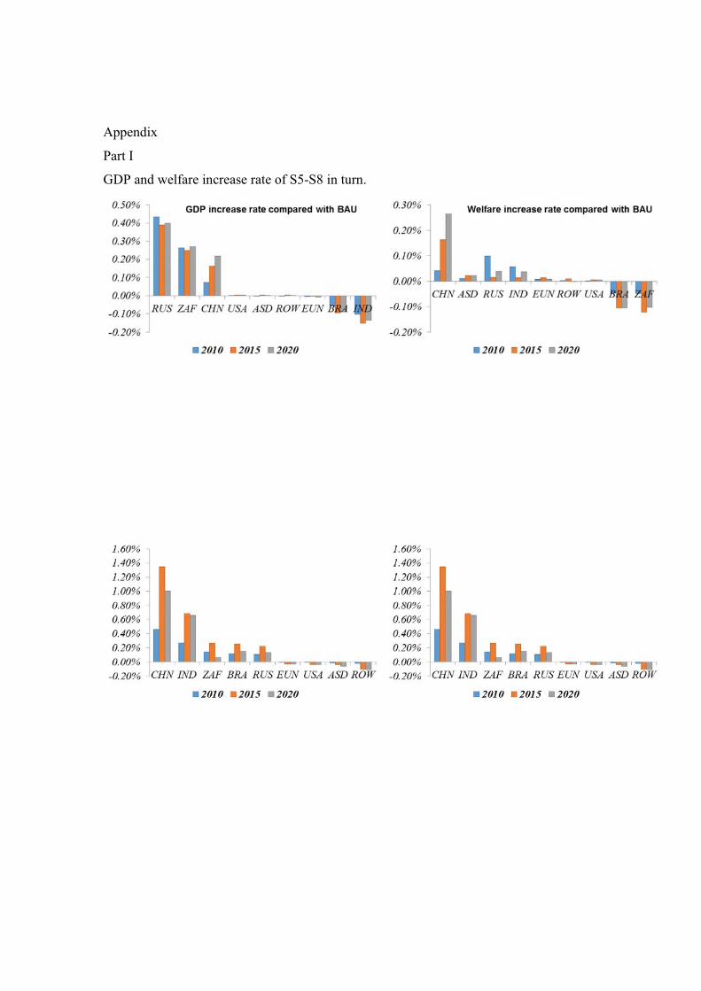
Appendix

Part I

GDP and welfare increase rate of S5-S8 in turn.

Export change rate of S5-S8 in BRICS

Part II Exchange rate of S1-S8 (compare with S0)