Как мне медведь на ухо наступил

ищем структуру в данных Last.fm

(Tone deaf: finding structure in Last.fm data)

Andrei Zhabinskihadoop engineer @ adform.com

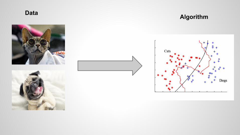
Data Algorithm

Data AlgorithmFeatures

“raw” features

name = fry

gender = male

age = 1029

height = 171

weight = 68

occupation = delivery boy

income = $510

balance = $4.3 billion

transformed / combined features

log(age) = 6.94

income^2 = 260100

height * weight = 11628

expert knowledge(domain specific)

planet(GeoIP) = Earth

working_hours(delivery boy) = 8

expert knowledge is really useful

Part-of-Speech TagsStemming/Lemmatization

Gabor filtersHaar waveletsSURF descriptors

but what if I’m not an expert?

Helps to find structure in “raw” data

Clustering

Principal Component Analysis

Autoencoders RBM

consider image data

raw pixel matrix structured patterns

deep learning

Images are too mainstream!

Last.Fm dataset 360K(http://mtg.upf.edu/node/1671)

● userid, artname, plays● data from 2001-2009● 360K unique users● 290K unique artists● 17M records

Most popularartname audience

1 radiohead 77348

2 the beatles 76339

3 coldplay 66738

4 red hot chili peppers 48989

5 muse 47015

6 metallica 45301

7 pink floyd 44506

8 the killers 41280

9 linkin park 39833

10 nirvana 39534

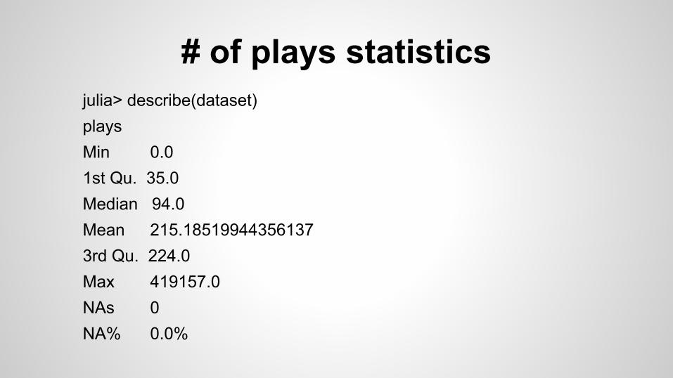
# of plays statisticsjulia> describe(dataset)playsMin 0.01st Qu. 35.0Median 94.0Mean 215.185199443561373rd Qu. 224.0Max 419157.0NAs 0NA% 0.0%

419157 * 3 min = 873 days

2.39 years

NOFX

Audience histogram

290K => 1K17M => 8M

Noisy and computationally hardLet’s reduce dataset

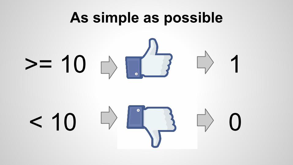
As simple as possible

>= 10

< 10

1

0

Like-matrixuser #1 user #2 ... user #n

artist #1 0 0 ... 1

artist #2 1 0 ... 0

... ... ... ... ...

artist #m 1 1 ... 0

Restricted Boltzmann Machines Two formulations:● neural network -

vertices are “neurons” connected via weighted edges

● Markov random field - vertices are random variables, edges show dependencies

feat

ure

#1

feat

ure

#2

feat

ure

#3

feat

ure

#4

“meg

a”-

feat

ure

#1

“meg

a”-

feat

ure

#2

“meg

a”-

feat

ure

#3

RBM “compresses” input, converting “raw” data into

more high-level representation

short probability theory review

Random Variable

Not a single value, but a set of values with associated

probabilities

Probability Distribution

X=0 X=1

0.3 0.7

probability distribution

X1=0 X1=1

X2=0 0.15 0.25

X2=1 0.4 0.3

joint probability distribution

Like-matrixuser #1 user #2 ... user #n

artist #1 0 0 ... 1

artist #2 1 0 ... 0

... ... ... ... ...

artist #m 1 1 ... 0

observation (object)

Like-matrixuser #1 user #2 ... user #n

artist #1 0 0 ... 1

artist #2 1 0 ... 0

... ... ... ... ...

artist #m 1 1 ... 0

binary random variable (feature)

artis

t #1

artis

t #2

artis

t #3

artis

t #4

? ? ? 2 sets of random variables:

● visible variables - we know their values (e.g. “likes”)

● hidden variables - some hidden counterparts of visible ones (genres? countries? decades?)

Ideally, we would like to get probability distribution table

V0 V1 V2 ... H1 H2 ... P(...)

0 0 0 ... 0 0 ... 0.002

0 0 0 ... 0 1 ... 0.0004

0 0 0 ... 1 0 ... 0.007

total number of combinations2^1100 =

13582985290493858492773514283592667786034938469317445497485196697278130927542418487205392083207560592298578262953847383475038725543234929971155548342800628721885763499406390331782864144164680730766837160526223176512798435772129956553355286032203080380775759732320198985094884004069116123084147875437183658467465148948790552744165

376L

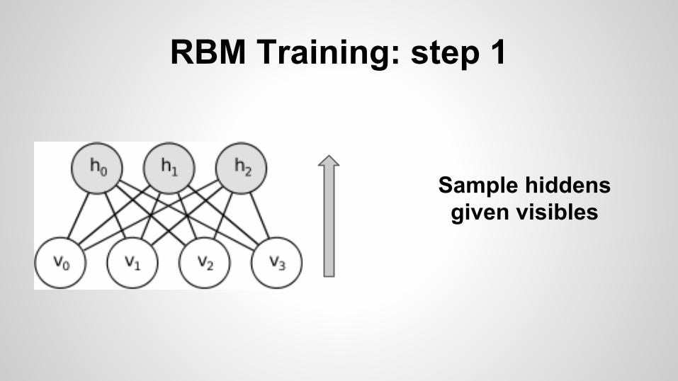
RBM Training: step 1

Sample hiddens given visibles

RBM Training: step 2

Sample visibles given hiddens (reconstruct)

RBM Training: step 3

Calculate error and adjust

weightsdW

training result - weight matrix that minimizes reconstruction error

Hidden variables after training

● each hidden units activates visible ones with different weights

● weights represent strength of some concepts

W1 W2 W3 W4

Learned concepts: pop / metal

VS.

Beyonce Metallica

Learned concepts: hard rock / epatage

VS.

Dream Theater Lady Gaga

Learned concepts: classic / alternative

VS.

Bob Dylan Linkin Park

Artist portrait

each artist may be described via weighted vector of concepts

Radiohead

axis weight

classic rock/grunge 0.23

pop/rock 0.24

electronic/country -0.23

pop rock/hard rock 0.37

hardcore/alternative -0.1

Artist portrait

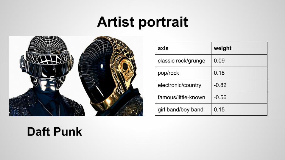
Daft Punk

axis weight

classic rock/grunge 0.09

pop/rock 0.18

electronic/country -0.82

famous/little-known -0.56

girl band/boy band 0.15

Artist portrait

RecommendationsFeatures

RecommendationsFeatures

RecommendationsFeatures

Questions?

https://github.com/dfdx