Title Simulation of Turbulent Diffusion and Reactive Flows by thePDF Methods (Turbulence Transport, Diffusion and Mixing)

Author(s) Sakai, Yasuhiko; Kubo, Takashi; Suzuki, Haruki

Citation 数理解析研究所講究録 (2003), 1339: 6-22

Issue Date 2003-09

URL http://hdl.handle.net/2433/43421

Right

Type Departmental Bulletin Paper

Textversion publisher

Kyoto University

Simulation of Turbulent Diffusion andReactive Flows by the PDF Methods

Yasuhiko SAKAI*1 , Ihffishi KUBO*1,*2 and Haruki SUZUKI*1

*1 :Department of Mechannformatics&Systems, Nagoya University,Furo cho, Chikusa-ku, Nagoya 464-8603, Japan

*2 (present) :Hitachi, Ltd, Mechanical Engeneering Research Laboratory,502, Kandatsu-cho, Tsuchiura, Ibaraki 300-0013, Japan

1 Introduction

Turbulent diffusion of matter and mixing phenomena with the chemical reaction are practicallyimportant in conection with many engineering and environmental problems. If the experimentsfor some specific turbulent diffusion or reactive flow phenomena would be planned, it apparentlyneeds very hard labor and alot of cost. On the other hand, the numerical simulations bycomputers have become effective to predict these phenomena because of the improvement ofcomputers and the development of numerical methods. Generally, there are Eulerian andLagrangian methods for the simulation of the turbulent diffusion field. In the present study,we adopted.the Lagrangian PDF (Probability Density Function) method (Pope, 1985, 1994;Dopazo, 1994) which is akind of Monte Carlo method. In the Lagrangian PDF method,the exact velocity-scalar joint PDF is approximated by the discrete PDF for aset of manystochastic particles, and the variations of velocity and scalar are modeled by the Lagrangianequation (See Pope, 1985, 1994; $\mathrm{D}\mathrm{o}\mathrm{p}\mathrm{a}\mathrm{z}\mathrm{o},1994$, for details of the method).

In this study, the following two fundamental problems of turbulent diffusion and reactiveflows have been investigated.(A) The reactive-scalar mixing layer in agrid-generated turbulence(B) The axisymmetric point source plume diffusion in aturbulent pipe flow

The first problem (A) has been studied experimentally by Bilger et al. (1991) for thegas phase and Komori et al. $(1993, 1994)$ for the liquid phase. Since the PDF method hasbeen mainly developed in the combusition engineering, there are still only alimited number ofresearches in the liquid phase (e.g. Pipino and Fox, 1994; Tsai and Fox, 1994). For this reason,we pay attention on the liquid phase reaction in the first problem (A). About the simulationof this problem, Komori et al. (1991) also proposed astochastic two particle model, but intheir model, it was assumed that the chemical reaction occurs when the distance between twoparticles becomes smaller than the Kolmogorov scale. Recently, Bilger (1993) and Klimenko(1990) have independently developed the conditional moment closure (CMC) model. In theCMC method, the information of mixture fraction is indispensable to get the unconditionalstatistics of the flow, and the Lagrangian PDF method is useful to predict the mixture fraction.In this study, to solve the first problem, the simplfied Langevin model (Pope, 1985) is used forthe velocity of stochastic particles. For the molecular mixing, three models: the Curl’s model(Curl, 1963), the modified Curl’s model (Dopazo, 1979; Janicka et al., 1979; Pope, 1982),and the binomial Langevin model ( $\mathrm{V}\mathrm{a}\mathrm{l}\mathrm{i}\tilde{\mathrm{n}}0$ and Dopazo, 1991) are adopted. The results arecompared with the experimental data in liquid phase (Komori et al., 1993, 1994).

数理解析研究所講究録 1339巻 2003年 6-22

6

With regard to the second problem (B), as the velocity model of the stochastic particles,ageneralized Langevin model expressed in the cylindrical coordinate system is adopted. Thegeneralized Langevin model was first proposed by Haworth and Pope (1986) and expressed inthe cylindrical coordinate system by Sakai et a1.(1999). This model is constructed to satisfy theconsistency condition of velocity field (Pope, and thermodynamic constraint (Sawford,1986). On the other hand, as the molecular mixing model, two models (i.e. the Dopazo’sdeterministic model (Dopazo, 1975) and the modified Curl’s model (Dopazo, 1979; Janicka etal., 1979; Pope, 1982)) are attempted. In this study, the scalar diffusion field from the pointsource at the center of the pipe is simulated and compared with experimental data by Beckeret al. (1966).

This paper is structured as follows: In the following Section, we recall the Langrangian PDFmethod as developed by Pope (1985), (1994) and by Dopazo (1994), and give the simulationresults of the reactive scalar mixing layer in the grid-turbulence of the liquid phase (Prob$\mathrm{l}\mathrm{e}\mathrm{m}(\mathrm{A}))$ . In Section 3, the simulation models and results of axisymmetric point source plumein afully developed turbulent pipe flow (Problem (B)) are given. In bothe Section 2and 3, theeffectiveness of the molecular mixing models used in this study is evaluated by comparing thesumulation results with the experimental data. In the last Section, we summarize the contentof this paper and make some remarks about our future works by the Lagrangian PDF method.

2Reactive-Scalar Mixing Layer in Grid-Turbulence(Problem (A))

2.1 Simulation Method

2.1.1 PDF Transport Equation

The transport equation for the velocity-scalar joint PDF $f(V, \psi;ox,t)$ in incompressible flow(Pope, 1985) is given by

$\frac{\partial f}{\partial t}+V_{j}\frac{\partial f}{\partial x_{j}}-\frac{1}{\rho}\frac{\partial(p\rangle}{\partial x_{j}}\frac{\partial f}{\partial V_{j}}+\frac{\partial}{\partial\psi_{\alpha}}(w_{\alpha}f)$

$= \frac{1}{\rho}\frac{\partial}{\partial V_{j}}[\langle-\frac{\partial\tau_{ij}}{\partial x}.\cdot+\frac{\partial p’}{\partial x_{j}}|V,\psi\rangle f]$

(1)$+ \frac{\partial}{\partial\psi_{\alpha}}[\langle\frac{\partial J^{\alpha}}{\partial x}\dot{.}\dot{.}|V,\psi\rangle f]$ ,

where $V$ and $\psi$ are sample spaces corresponding to the velocity $U$ and the concentration $\Gamma$ ,respectively, and $x$ is the position in the physical space, $t$ is the time, $\rho$ is the density, $p$ is thepressure, $w_{\alpha}$ is the chemical source term for species $\alpha$ , $\tau_{ij}$ is the viscous stress tensor, and $J_{i}^{\alpha}$

is the diffusive flux vector for species $\alpha$ . $\langle Q|V,\psi\rangle$ stands for the conditional expectation of $Q$ ,given that $U(ax, t)=V$ and $\Gamma(ax, t)=\psi$ , where $Q=\mathrm{Q}\{\mathrm{U},$ $\Gamma$) is afunction of $U$ and $\Gamma$ .

The terms on the left-hand side of Eq.(l) represent the unsteady term, the transport inthe physical space, the transport in the velocity space by the mean pressure gradient, and thetransport in the scalar space by the reaction, respectively. All these terms can be treated with-out approximation. The terms on the right-hand side of Eq.(l) stand for the transport in thevelocity space by the viscous stress and by the fluctuating pressure gradient and the transportin the scalar space by the molecular fluxes. These terms including conditional expectationsmust be modeled.

In the Lagrangian PDF method, the velocity-scalar joint PDF within the solution domain,$f(V,\psi;ax,t)$ , is approximated by $N(t)$ stochastic particles. The state of the $n\mathrm{t}\mathrm{h}$ stochastic

7

particle at time $t$ is represented by

$U^{(n)}(t)$ , $\Gamma^{(n)}(t)$ , $ox^{(n)}(t)$ $(n=1,2, \ldots, N(t))$ . (2)

The discrete PDF of the stochastic particle is defined by

$f_{N}(V, \psi;ox,t)=\frac{1}{N}\sum_{n=1}^{N}\delta(V-U^{(n)})\delta(\psi-\Gamma^{(n)})\delta(ox-x^{(n)})$, (3)

and the relation between the discrete PDF $f_{N}$ and the true PDF $f$ is

$f(V, \psi;x, t)=\langle f_{N}(V,\psi;x, t)\rangle$ , (4)

i.e., the expectation of the discrete PDF is the true PDF (Pope, 1985).The modeled joint PDF equation is solved numerically by integrating the state of the

stochastic particles under the given initial and boundary conditions. The Lagrangian PDFsimulation is one of the Monte Carlo methods. In the following, the models of the velocity andconcentration of the stochastic particles used in the Problem (A) are given.

2.1.2 Velocity

Since the mixing layer in agrid-generated turbulence is considered in this study, the velocityof the stochastic particle is modeled by the following simplified Langevin model (Pope, 1985),

$dU_{\dot{l}}^{(n)}=-( \frac{1}{2}+\frac{3}{4}C\mathrm{o})(U_{i}^{(n)}-\langle U_{\dot{1}}\rangle)\frac{dt}{\tau}+(C0\epsilon)^{1/2}dW_{\dot{l}}$, (5)

where $dU_{\dot{1}}$ $=U_{\dot{\iota}}(t+dt)-U_{\dot{\iota}}(t)$ , the increment of velocity; $dt$ , the time increment; $C_{0}$ , Kolmogorovconstant; $\epsilon$ , the dissipation rate of the turbulent kinetic energy per unit mass $k;\tau$ , the timescale of turbulence $\tau=k/\epsilon;dW${, the increment of isotropic Wiener process with zero meanand covariance $(dW_{}dW_{j}\rangle=dt\delta_{ij}$ .

2.1.3 Molecular Mixing Model

Three fundamental models: the Curl’s model (Curl, 1963), the modified Curl’s model (Dopazo,1974; Janika et al., 1979; Pope, 1982) and the binomial Langevin model ($\mathrm{V}\mathrm{a}\mathrm{l}\mathrm{i}\tilde{\mathrm{n}}0$ and Dopazo,1991) are used. Each model is explained in the following.

Curl’s Model For the Curl’s model (Curl, 1963), in the small interval $dt$ the probabilityof the yith particle being mixed is given by

$P^{(n)}= \frac{2C_{\phi}dt}{\tau(x^{(n)}(t))}$ , (6)

where $C_{\phi}=\tau/\tau_{\phi}$ is the empirical constant and $\tau_{\phi}$ is the time scale of molecular mixing. Whenthe mixing takes place with this probability, the pair to the yzth particle is selected (here, theryrth particle) and the concentrations of two particles are replaced by their mean:

$\Gamma_{\alpha}^{(n)}(t+dt)=\Gamma_{\alpha}^{(m)}(t+dt)=\frac{1}{2}(\Gamma_{\alpha}^{(n)}+\Gamma_{\alpha}^{(m)})$ , (7)

where the right-hand side of Eq.(7) represents the state at time $t$ . The nearest stochasticparticle is selected as apair because mixing takes place locally in the physical space

8

Modified Curl’s Model In the modified Curl’s model (Dopazo, 1979; Janicka et al.,1979; Pope, 1982), the probability of the particle being mixed is modified by

$P^{(n)}= \frac{3C_{\phi}dt}{\tau(x^{(n)}(t))}$ , (8)

and the concentrations of pair particles are replaced by

$\Gamma_{\alpha}^{(n)}(t+dt)=(1-\beta)\Gamma_{\alpha}^{(n)}+\frac{1}{2}\beta(\Gamma_{\alpha}^{(n)}+\Gamma_{\alpha}^{(m)})$ , (9a)

$\Gamma_{\alpha}^{(m)}(t+dt)=(1-\beta)\Gamma_{\alpha}^{(m)}+\frac{1}{2}\beta(\Gamma_{\alpha}^{(n)}+\Gamma_{\alpha}^{(m)})$ , (9b)

where $\beta$ is arandom variable uniformly distributed on the interval $[0,1]$ . $\beta$ represents the degreeof mixing in aparticle pair; no mixing occurs with $\beta$ $=0$, and the Curl’s model is recoveredwith $\beta=1$ .

Binomial Langevin Model Valino and Dopazo (1991) proposed the following binomialLangevin model,

$d\Gamma^{(n)}$$=$ $- \frac{1}{2}[1+K(1-\frac{\langle\gamma^{\prime 2})}{\gamma_{*}^{2}},)]\frac{C_{\phi}}{\tau}(\Gamma^{(n)}-\langle\Gamma\rangle)dt$

(11)$+[K(1- \frac{(\gamma^{\prime(n)})^{2}}{\gamma_{*}^{2}},)\frac{C_{\phi}}{\tau}(\gamma^{\prime 2}\rangle dt]1/2\xi_{\mathrm{b}\mathrm{i}\mathrm{n}}$,

where $K$ , aconstant; $\xi_{\mathrm{b}\mathrm{i}\mathrm{n}}$ , anormalized binomially distributed random variable; and the primerepresents the fluctuation value. $\gamma_{*}’$ is equal to $\gamma_{\max}’$ if $\gamma^{\prime(n)}$ is positive and equal to $\sqrt\min$

if $\gamma^{\prime(n)}$ is negative, where subscripts $\max$ and $\min$ are the allowable maximum and minimumfluctuation, respectively. $\xi_{\mathrm{b}\mathrm{i}\mathrm{n}}$ is generated to preserve the boundedness of the scalar concen-tration.

2.1.4 Position and Chemical Reaction

The position of the stochastic particles in the physical space and the chemical source termare treated without modeling. This is an advantage in the Lagrangian PDF method used inthis study. Therefore, the changes of position and concentration by the chemical reaction arecalculated as follows,

$dx_{i}$ $=$ $U_{\dot{1}}dt$ , (11)$d\Gamma_{\alpha}$ $=$ $w_{\alpha}dt$ . (12)

2.2 Simulation Conditions

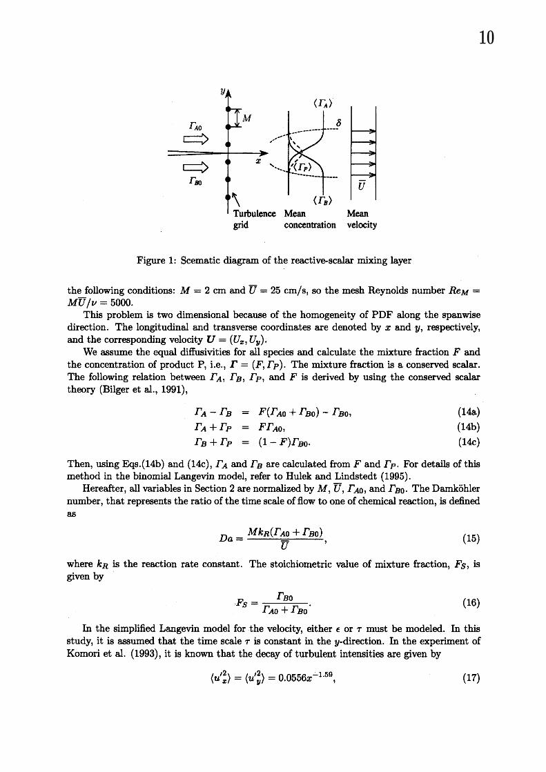
Figure 1shows aschematic diagram of the reactive-scalar mixing layer simulated in this study.Nonpremixed species Aand $\mathrm{B}$ are supplied from the upstream of the grid with the mesh sizeof $M$ , at the constant velocity U. The initial concentrations of species Aand $\mathrm{B}$ are $\Gamma_{A0}$ and$\Gamma_{B0}$ , respectively. The second order and irreversible chemical reaction:

$\mathrm{A}+\mathrm{B}arrow \mathrm{P}$ (13)

has occurred in the mixing region of species Aand $\mathrm{B}$ , where species $\mathrm{P}$ is produced in thedownstream of the grid. The experiments of Komori et al. $(1993, 1994)$ were conducted unde

9

grid concentration velocity

Figure 1: Scematic diagram of the reactive-scalar mixing layer

the following conditions: $M=2$ cm and $\overline{U}=25\mathrm{c}\mathrm{m}/\mathrm{s}$, so the mesh Reynolds number $Re_{M}=$

$M\overline{U}/\nu=5000$ .This problem is two dimensional because of the homogeneity of PDF along the spanwise

direction. The longitudinal and transverse coordinates are denoted by $x$ and $y$ , respectively,and the corresponding velocity $U=(U_{x}, U_{y})$ .

We assume the equal diffusivities for all species and calculate the mixture ffaction $F$ andthe concentration of product $\mathrm{P}$, i.e., $\Gamma=(F, \Gamma P)$ . The mixture fraction is aconserved scalar.The following relation between Fa, $\Gamma_{B}$ , $\Gamma_{P}$ , and $F$ is derived by using the conserved scalartheory (Bilger et al., 1991),

$\Gamma_{A}-\Gamma_{B}$ $=$ $F(\Gamma_{A0}+\Gamma_{B0})-\Gamma_{B0}$ , (14a)$\Gamma_{A}+\Gamma_{P}$ $=$ $F\Gamma_{A0}$ , (14b)$\Gamma_{B}+\Gamma_{P}$ $=$ $(1-F)\Gamma_{B0}$ . (14c)

Then, using Eqs.(14b) and (14c), $\Gamma_{A}$ and $\Gamma_{B}$ are calculated from $F$ and $\Gamma_{P}$ . For details of thismethod in the binomial Langevin model, refer to Hulek and Lindstedt (1995).

Hereafter, all variables in Section 2are normalized by $M$ , $\overline{U}$ , $\Gamma_{A0}$ , and $\Gamma_{B0}$ . The Damkohlernumber, that represents the ratio of the time scale of flow to one of chemical reaction, is definedas

$Da= \frac{Mk_{R}(\Gamma_{A0}+\Gamma_{B0})}{\overline{U}}$ , (15)

where $k_{R}$ is the reaction rate constant. The stoichiometric value of mixture fraction, $F5$ , isgiven by

$F_{S}= \frac{\Gamma_{B0}}{\Gamma_{A0}+\Gamma_{B0}}$. (16)

In the simplified Langevin model for the velocity, either $\epsilon$ or $dr$ must be modeled. In thisstudy, it is assumed that the time scale $\tau$ is constant in the $y$-direction. In the experiment ofKomori et al. (1993), it is known that the decay of turbulent intensities are given by

$\langle u_{x}^{\prime 2}\rangle=\langle u_{y}^{\prime 2}\rangle=0.0556x^{-1.59}$ , (15)

10

so here $\tau$ is modeled to increase linearly in the downstream direction:

$\tau=\frac{k}{\epsilon}=(\frac{3}{2}\langle u_{x}^{\prime 2}\rangle)/(-\frac{3}{2}\frac{d\langle u_{x}^{\prime 2}\rangle}{dx})=0.629x$. (18)

Kolmogorov constant can be related to the turbulent diffusion coefficient through the Lagrangian time scale $T_{L}$ :

$T_{L}= \frac{4}{3C_{0}}\tau$ . (19)

Kolmogorov constant is assumed to be $C_{0}=1.1$ in such away that the mixing layer thicknessagrees with the experimental data. It is smaller than the value used by Pope (1985), $C_{0}=2.1$ ,probably because the Reynolds number of the experiments by Komori et al. $(1993, 1994)$ israther small.

The empirical constant, $C_{\phi}$ , is adjusted to be 0.44 in such amanner as the decay of con-centration fluctuation agrees with the experimental data. Although we assume that $C_{\phi}$ isconstant, it is known that the value of $C_{\phi}$ depends on the modeling of molecular mixing timescale $\tau_{\phi}$ . For example, using Corrsin’s model (1964), $C_{\phi}$ varies in the downstream direction andits value is between 0.5-0.6 in the simulation region. Recently, Pipino and Fox (1994) proposedthe spectral relaxation model and showed its advantage.

According to Valino and Dopazo (1991), $K=2.1$ is chosen in the binomial Langevinmodel for the concentration. The simulation has been made for the finite Damkohler number,$Da=0.752$ , corresponding to the moderately fast reaction in the experiment of Komori et al.(1994) $(k_{R}=0.047\mathrm{m}^{3}/(\mathrm{m}\mathrm{o}1\cdot \mathrm{s}), \Gamma_{A0}=\Gamma_{B0}=100\mathrm{m}\mathrm{o}1/\mathrm{m}^{3})$.

The frozen limit ($Daarrow \mathrm{O}$, corresponding to no reaction) and equilibrium limit $(Daarrow\infty$,corresponding to the instantaneous reaction) are determined by using the conserved scalartheory (Bilger et al., 1991) as follows.

As $Daarrow 0$,

$\lim_{Daarrow 0}\Gamma_{A}$$=$ $F$, (20)

$\lim_{Daarrow 0}\Gamma_{B}$$=$ 1-F. (21)

As $Daarrow\infty$ ,

$\lim_{Daarrow\infty}\Gamma_{A}$$=$ $\frac{F-F_{S}}{1-F_{S}}H(F-F_{S})$ , (22)

$\lim_{Daarrow\infty}\Gamma_{B}$$=$ $\frac{F_{S}-F}{F_{S}}H(F_{S}-F)$ . (23)

where $H$ is the Heaviside unit step function.The solution in the domain $2\leq x\leq 20,$ $-2.5\leq y\leq 2.5$ is calculated by amarching solution

method (Pope, 1985). In this method, the constant spatial increment, $dx=1/1\mathrm{O}\mathrm{O}$ , is related tothe time increment of stochastic particle, $dt^{(n)}=dx/U_{x}^{(n)}$ . The number of stochastic particlesis $N=400,000$ and various expectations are calculated in the small region, $dy=0.1$ .

With regard to the initial conditions, the stochastic particles are uniformly distributedin the $y$-direction at $x=2$, the velocities of them are generated as Eq.(17) is satisfied, andconcentrations of them are set to be,

$\Gamma_{A}$ $=$ 1, $\Gamma_{B}=0$ , for $y>0$ (24a)$\Gamma_{A}$ $=$ 0, $\Gamma_{B}=1$ . for $y<0$ (24b)

For the boundary condition, we adopt aperfect reflection of stochastic particles at $|y|=2.5$

11

2.3 Simulation Result

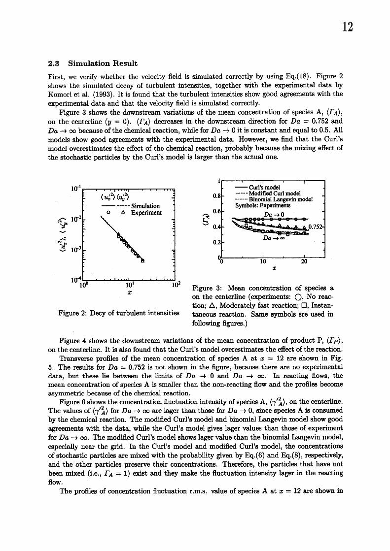
First, we verify whether the velocity field is simulated correctly by using Eq.(18). Figure 2shows the simulated decay of turbulent intensities, together with the experimental data byKomori et al. (1993). It is found that the turbulent intensities show good agreements with theexperimental data and that the velocity field is simulated correctly.

Figure 3shows the downstream variations of the mean concentration of species $\mathrm{A}$ , $\langle\Gamma A)$ ,on the centerline $(y=0)$ . $\langle\Gamma A\rangle$ decreases in the downstream direction for $Da=0.752$ and$Daarrow\infty$ because of the chemical reaction, while for $Daarrow \mathrm{O}$ it is constant and equal to 0.5. Allmodels show good agreements with the experimental data. However, we find that the Curl’smodel overestimates the effect of the chemical reaction, probably because the mixing effect ofthe stochastic particles by the Curl’s model is larger than the actual one.

$\mathrm{c}\hat{\underline{\mathrm{e}}_{\mathrm{S}^{\theta}}\vee}$

$\hat{\vee \mathrm{b}^{\triangleleft}}$

$\hat{\mathrm{r}_{\tilde{\vee}}3^{\mathrm{B}}}$

.

$x$

Figure 3: Mean concentration of species a$x$

on the centerline (experiments: $\mathrm{O}$ , No reac-than $\triangle$ , Moderately fast reaction; Cl, Instan-

Figure 2: Decy of turbulent intensities taneous reaction. Same symbols sre used infolowing figures.)

Figure 4shows the downstream variations of the mean concentration of product $\mathrm{P}$, $(\Gamma_{P}\rangle$ ,on the centerline. It is also found that the Curl’s model overestimates the effect of the reaction.

Transverse profiles of the mean concentration of species Aat $x=12$ are shown in Fig.5. The results for $Da=0.752$ is not shown in the figure, because there are no experimentaldata, but these lie between the limits of $Daarrow \mathrm{O}$ and $Daarrow\infty$ . In reacting flows, themean concentration of species Ais smaller than the non-reacting flow and the profiles becomeasymmetric because of the chemical reaction.

Figure 6shows the concentration fluctuation intensity of species $\mathrm{A}$ , $\langle\sqrt{}^{2}A\rangle$ , on the centerline.The values of $\langle\gamma_{A}^{\prime 2}\rangle$ for $Daarrow\infty$ are lager than those for $Daarrow \mathrm{O}$ , since species Ais consumedby the chemical reaction. The modified Curl’s model and binomial Langevin model show goodagreements with the data, while the Curl’s model gives lager values than those of experimentfor $Daarrow\infty$ . The modified Curl’s model shows lager value than the binomial Langevin model,especially near the grid. In the Curl’s model and modified Curl’s model, the concentrationsof stochastic particles are mixed with the probability given by Eq.(6) and Eq.(8), respectively,and the other particles preserve their concentrations. Therefore, the particles that have notbeen mixed (i.e., $\mathrm{r}_{A}=1$ ) exist and they make the fluctuation intensity lager in the reactingflow.

The profiles of concentration fluctuation r.m.s. value of species Aat $x=12$ are shown in

12

$\hat{\vee \mathrm{b}^{\mathrm{k}}}$

$\hat{\vee \mathrm{t}^{\mathrm{H}}}$

$x$

$y$

Figure 4: Mean concentration of product Figure 5: Mean concentration profiles of$\mathrm{P}$ on the centerline species Aat $x=12$ .

Fig. 7. For $Daarrow\infty$ , the r.m.s. value gives the peak in the region $y>0$ , where the reactantAexists in excess, and the peak value becomes lager than one for $Daarrow \mathrm{O}$ by the effect ofthe chemical reaction. The Curl’s model and modified Curl model show lager value than thebinomial Langevin model in the region $y<0$ for $Daarrow\infty$ . It is probably caused by the effectof the particles that have not been mixed.

$\frac{\sim}{\hat{\sim}}.\backslash \tau$

$\vee\succ$

$x$

Figure 6: Concentration fluctuation Figure 7: Profiles of concentration fluctuationintensity of species Aon the centerline r.m.s. value of species Aat $x=12$ .

Figure 8shows the concentration correlation coefficient between species Aand $\mathrm{B}$ , $R_{AB}$ , onthe centerline. $R_{AB}=1$ in the case of $Daarrow \mathrm{O}$ , since concentration fluctuation $\gamma_{A}’=-\gamma_{B}’$ .$R_{AB}$ increases in the downstream direction by the chemical reaction. It is found that the Curl’smodel overestimates the effect of the reaction and that the modified Curl’s model and binomialLangevin model show good agreements with the experimental data.

Figure 9shows the segregation coefficient, $at=\langle\gamma_{A}\gamma_{B}$) $/(\langle\Gamma A\rangle\langle\Gamma_{B}\rangle)$ , on the centerline. $\alpha$

indicates the degree of the coexistence between species Aand B. We can easily find $\alpha=0$

if species are mixed completely, and $\alpha=-1$ if there is no mixing. For $Daarrow \mathrm{O}$ , $\alpha$ increasesgradually, because the mixing proceeds in the downstream. For $Daarrow\infty$ , $\alpha=-1$ , since

13

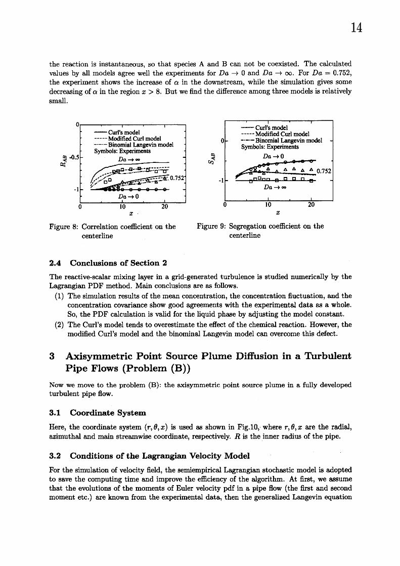
the reaction is instantaneous, so that species Aand $\mathrm{B}$ can not be coexisted. The calculatedvalues by all models agree well the experiments for $Daarrow \mathrm{O}$ and $Daarrow\infty$ . For $Da=0.752$ ,the experiment shows the increase of $\alpha$ in the downstream, while the simulation gives somedecreasing of $\alpha$ in the region $x>8$ . But we find the difference among three models is relativelysmall.

$\mathit{0}\grave{e}\mathrm{Q}$

$a_{)}^{T}\mathrm{r}$

$x$ $x$

Figure 8: Correlation coefficient on the Figure 9: Segregation coefficient on thecenterline centerline

2.4 Conclusions of Section 2the reaction calar mixing layer in agrid-generated turbulence is studied numerically by theLagrangian PDF method. Main conclusions are as follows.

(1) The simulation results of the mean concentration, the concentration fluctuation, and theconcentration covariance show good agreements with the experimental data as awhole.So, the PDF calculation is valid for the liquid phase by adjusting the model constant.

(2) The Curl’s model tends to overestimate the effect of the chemical reaction. However, themodified Curl’s model and the binominal Langevin model can overcome this defect.

3Axisymmetric Point Source Plume Diffusion in aTurbulentPipe Flows (Problem (B))

Now we move to the problem (B): the axisymmetric point source plume in afully developedturbulent pipe flow.

3.1 Coordinate System

Here, the coordinate system $(r, \theta,x)$ is used as shown in Fig.lO, where $\mathrm{r},0,\mathrm{x}$ are the radial,azimuthal and main streamwise coordinate, respectively. $R$ is the inner radius of the pipe.

3.2 Conditions of the Lagrangian Velocity Model

For the simulation of velocity field, the semiempirical Lagrangian stochastic model is adoptedto save the computing time and improve the efficiency of the algorithm. At first, we assumethat the evolutions of the moments of Euler velocity pdf in apipe flow (the first and secondmoment etc.) are known from the experimental data, then the generalized Langevin equation

14

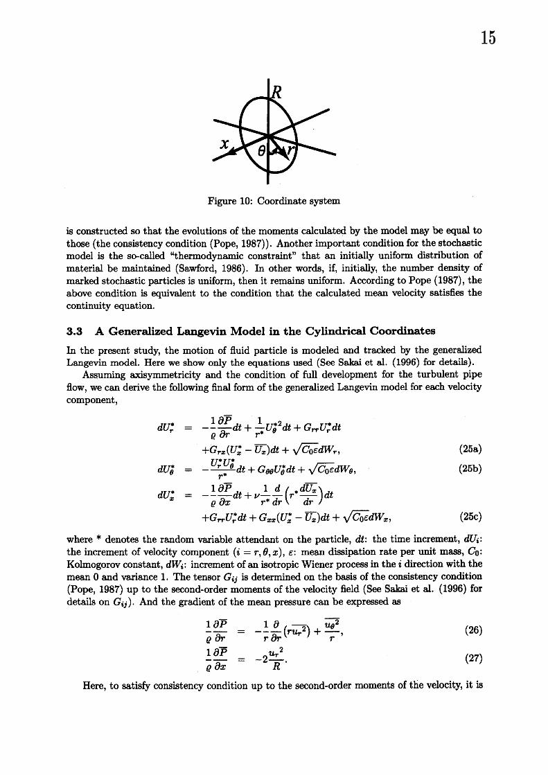
Figure 10: Coordinate system

is constructed so that the evolutions of the moments calculated by the model may be equal tothose (the consistency condition (Pope, 1987)). Another important condition for the stochasticmodel is the s0-called “thermodynamic constraint” that an initially uniform distribution ofmaterial be maintained (Sawford, 1986). In other words, if, initially, the number density ofmarked stochastic particles is uniform, then it remains uniform. According to Pope (1987), theabove condition is equivalent to the condition that the calculated mean velocity satisfies thecontinuity equation.

3.3 AGeneralized Langevin Model in the Cylindrical Coordinates

In the present study, the motion of fluid particle is modeled and tracked by the generalizedLangevin model. Here we show only the equations used (See Sakai et al. (1996) for details).

Assuming axisymmetricity and the condition of full development for the turbulent pipeflow, we can derive the following final form of the generalized Langevin model for each velocitycomponent,

$dU_{f}^{*}$ $=$ $- \frac{1}{\rho}\frac{\partial\overline{P}}{\partial r}dt+\frac{1}{r^{*}}U_{\theta}^{*2}dt+G_{rr}U_{f}^{*}dt$

$+G_{rx}(U_{x}^{*}-\overline{U_{x}})dt+\sqrt{C_{0}\epsilon}dW_{r}$ , (25a)

$dU_{\theta}^{*}$ $=$ $- \frac{U_{r}^{*}U_{\theta}^{*}}{r^{*}}dt+G_{\theta\theta}U_{\theta}^{*}dt$ $+\sqrt{C_{0}\epsilon}dW\theta$ , (25b)

$dU_{x}^{*}$ $=$ $- \frac{1}{\rho}\frac{\partial\overline{P}}{\partial x}dt+\nu\frac{1}{r^{*}}\frac{d}{dr}(r^{*}\frac{d\overline{U_{x}}}{dr})dt$

$+G_{tt}U_{r}^{*}dt+G_{xxx}(U_{x}^{*}-\overline{U_{x}})dt+\sqrt{C0\epsilon}dW_{x}$ , (25c)

$\mathrm{w}\mathrm{h}\mathrm{e}\mathrm{r}\mathrm{e}\mathrm{d}*\mathrm{e}\mathrm{n}\mathrm{o}\mathrm{t}\mathrm{e}\mathrm{s}$ the random variable attendant on the particle, $dt$ :the time increment, $dU\dot{.}$ :the increment of velocity component $(i=r, \theta, x)$ , $\epsilon$:mean dissipation rate per unit mass, Co:Kolmogorov constant, $\mathrm{d}\mathrm{W}\mathrm{i}$ :increment of an isotropic Wiener process in the $i$ direction with themean 0and variance 1. The tensor $G_{\dot{|}j}$ is determined on the basis of the consistency condition(Pope, 1987) up to the second-0rder moments of the velocity field (See Sakai et al. (1996) fordetails on $G_{ij}$ ). And the gradient of the mean pressure can be expressed as

$\frac{1}{\rho}\frac{\partial\overline{P}}{\partial r}$ $=$$- \frac{1}{r}\frac{\partial}{\partial r}(r\overline{\mathrm{u}_{f}^{2}})\dagger\overline{\frac{u_{\theta^{2}}}{r}}$ , (26)

$\frac{1}{\rho}\frac{\partial\overline{P}}{\partial x}$ $=$ $-2 \frac{u_{\tau}^{2}}{R}$ . (27)

Here, to satisfy consistency condition up to the second-0rder moments of the velocity, it is

15

necessary to specify the radial distributions of the following mean quantities up to the third-order,

Second-0rder momentsFirst-0rder moment

$.\cdot.\cdot.\cdot$

$\overline{\frac{\frac{U_{x}}{u_{r^{2}}}}{u_{r^{3}}}},’\frac{\overline u_{\theta^{2}},u}{u_{r^{2}}u_{x}},’\frac{\overline{2}\overline{u_{r}}}{u_{r}u_{\theta^{2}}}xu_{x},\overline{u_{r}u_{x^{2}}}$

, $\overline{u_{\theta^{2}}u_{x}}$Third-0rder momentsmean dissipation rate per unit mass : $\epsilon$

In the following, we explain the way of giving these parameters. Firstly, the radial distributionof the mean velocity is given by the following equation in which the wake function (Tennekesand Lumley, 1972) is added to the equation of mean velocity by Reichardt (See Hinze, 1975),

$\overline{\frac{U_{x}}{u_{\tau}}}$ $= \frac{1}{\kappa}\ln(1+\kappa y^{+})+c[1-\exp(-\frac{y^{+}}{\delta_{l^{+}}})-\frac{y^{+}}{\delta_{l^{+}}}\exp(-0.33y^{+})]$

$+d[1- \cos(\pi\frac{y}{\delta})]$ ,

$\kappa$ $=0.4$ , $c=6.0$, $\delta_{l^{+}}=11.0$ , $d=0.5$, $\delta=0.77R$ , (28)

where $y^{+}=u_{\tau}y/\nu$($y:\mathrm{d}\mathrm{i}\mathrm{s}\mathrm{t}\mathrm{a}\mathrm{n}\mathrm{c}\mathrm{e}$ from the wall; $y=R-r$) and the third term of the right-handside is the wake function. The parameters $c$ and $\delta$ are chosen for the mean velocity at thecenter of the pipe $\overline{U_{c}}$ and the cross-sectional mean velocity $U_{av}$ to agree with those given byBecker et al. (1966). The experimental study by Becker et al. is the subject of the simulationin the present research.

With regard to the second-0rder moments, i.e. $\overline{u_{f}^{2}},\overline{u_{\theta}^{2}}$ and $\overline{u_{x}^{2}}$ and the mean dissipation rate$\epsilon$ , Laufer(1954)’s data (Reynolds number ${\rm Re}_{c}=2R\overline{U_{c}}/\nu=500,000$ ) are used. Here it is noted thatthe Reynolds number of Laufer’s experiment is different ffom that of the experiment by Beckeret al. (1966) ( ${\rm Re}_{\mathrm{c}}=2R\overline{U_{\mathrm{c}}}/\nu=796,000$;This value corresponds to ${\rm Re}=2RU_{av}/\nu=684,000$). How-ever, both Rec are in the same order, so distributions of the second moments and the meandissipation rate are not so different with each other. From this reason, the Laufer’s experimen-tal results are used as the specified data.

The Reynolds stress $\overline{u_{r}u_{x}}$ is readily determined by integrating the $x$-direction mean velocityequation, which is given by

$\overline{u_{r}u_{x}}=\nu\frac{\partial\overline{U_{x}}}{\partial r}+\frac{u_{\tau}^{2}}{R}r$. (29)

With regard to the third-0rder moments of the velocity, although there exist Laufer’s exper-imental data, the scattering of the data is quite large. Thus, we judged that those data are notsuitable for inputting to the present model, and decided to omit the input of the third-0rdermoments to the model. This means that the present model does not satisfy the consistencycondition exactly. Thus we need to check the consistency condition in the practical simulationin order judge whether the present model gives us reliable results or not. This check is madeby comparing the calculated statistics of the velocity field with the experimental (prescribed)data.

3.4 Molecular Mixing Model

In the present problem, the DOpazO(1975)’s deterministic model and the modified Curl’smodel(Dopazo, 1975; Janicka et $\mathrm{a}1$ , 1979; Pope, 1982) are adopted as the molecular mixin

16

model. The modified Curl’s model has been already explained in \S 2.1.3. In the following, weexplain the Dopazo’s model.

3.4.1 Dopazo’s Deterministic Model.

In the Dopazo’s deterministic model (Dopazo, 1975), when the scalar (concentration) attendanton the particle is represented by $\Gamma$ , the increment of the scalar $d\Gamma$ is given by

$d\Gamma$ $=- \frac{1}{2}C_{\phi}(\Gamma-\langle\Gamma\rangle)\frac{dt}{\tau}$ , (30)

where ( $\Gamma\rangle$ is the ensemble average of the scalar over particles within each cell which is fixed onthe spatial area. $C_{\phi}$ is the parameter which determines the decay rate of the variance of thescalar. And $\tau$ is the turbulent time scale, which is defined by

$\tau=\frac{\kappa}{\epsilon}$ , $\kappa$

$= \frac{\overline{u_{r^{2}}}+\overline{u_{\theta^{2}}}+\overline{u_{x^{2}}}}{2}$, (31)

where $\kappa$ is the turbulent kinetic energy, $\epsilon$ is the dissipation rate of $\kappa$ . In this model, the scalarattendant on the particle is determined not randomly but deterministicaly.

3.5 Simulation Conditions

The subject of the present simulation is the oil fog diffusion field by Becker et al. (1966).The simulation conditions are adjusted to those of the experiments by Becker et al.. In theexperiments, the measurements of the concentration field of the point source plume of oil fogwhich is injected from the center of the pipe in afully developed turbulent pipe flow weremade. The fog injector’s inner diameter is 2.16 $\mathrm{m}\mathrm{m}$, and the outer diameter is 2.77 $\mathrm{m}\mathrm{m}$ . In theactual experiments, the measurement points were fixed and the injector was moved, then theconcentrations were measured at the several downstream cross sections from the injector’s exit(the plume source). On the other hand, we fixed the plume source at the origin and calculatedconcentrations at the same downstream distances from the source as those of experiments.Further, Becker et al. performed the experiments for several values of $\overline{U_{c}}$, but in this studywe chose only one case of these experiments as the simulation subject: the case of $\overline{U_{\mathrm{c}}}=61\mathrm{m}/\mathrm{s}$

$({\rm Re}=684,000)$ . The conditions of the simulation are as follows.

inner radius of the pipe : $R=0.1005$ $\mathrm{m}$

cross-sectional mean velocity : $U_{av}=52.38$ $\mathrm{m}/\mathrm{s}$

kinematic viscosity : $\nu=1.54\mathrm{x}10^{-5}\mathrm{m}^{2}/\mathrm{s}$

Reynolds number : ${\rm Re}=2RU_{av}/\nu=684,000$

friction velocity : $u_{\tau}=2.15\mathrm{m}/\mathrm{s}$

Kolmogorov constant : $C_{0}=2.0$

boundary condition absorptive wall

3.6 Simulation Results

3.6.1 Verification of the Velocity Field

Firstly, we made the numerical verifications of the consistency condition (Pope, 1987) up tothe second-0rder moment and the thermodynamic constraint (Sawford, 1986) for the calcu-lated velocity field. Since the subject of calculation is afully developed turbulence field and

17

the velocity field is independent of the azimuthal-direction, only the radial movements of theparticles were calculated in this verification. Although the figures are not shown here becauseof the limitation of the paper length, it was confirmed that the velocity field simulated by thepresent model can reproduce well the prescribed data up to the second-0rder moment even ifthe input of the third-0rder moment is omitted. This gives us some practical background torely on the simulation of the scalar diffusion problem shown in the following section. Further,it was also ascertained that the initial uniform distribution of stochastic particles is almostunchanged with time in the simulation. Thus we concluded that the velocity field simulatedby the present model satisfies the thermodynamic constraint, i.e., the continuity condition(Sawford, 1986).

3.6.2 Scalar Diffusion from the Center of the Pipe

For the simulation of the scalar field, the two dimensional calculation of the radial and mainstreamwise direction was made because of the axisymmetricity of the pipe. Thus, the distanceof the particle movement in the radial and main streamwise direction $dr^{*}$ , $dx^{*}$ during the timeincrement $dt$ is calculated by

$dr^{*}$ $=U_{r}^{*}dt$, (32)$dx^{*}$ $=U_{x}^{*}dt$ . (33)

First, at the initial time the particles are distributed uniformly over the area of the calculation$(r=0\sim R,x=0\sim 7.0R)$ and the particles within the source are given the scalar valueof 1, the others are given the scalar value of 0. The change of the scalar attendant on eachparticle is calculated by the molecular mixing model mentioned in the previous section. Thesize of the source is $0.04R$ in both the radial direction and the main streamwise direction.This size was determined on the basis of the empirical equation of the mixing length given byNikuradse(see $\mathrm{S}\mathrm{c}\mathrm{h}\mathrm{l}\mathrm{i}\mathrm{c}\mathrm{h}\mathrm{t}\mathrm{i}\mathrm{n}\mathrm{g},1979$ ). The total number of particles is $N_{t}=2,000,000$ , the timeincrement is $dt=4.67\mathrm{x}10^{-6}\sec$ for one step, and the total number of time steps is 11,000,which corresponds to the real time of 5.137 $\mathrm{x}10^{-2}\mathrm{s}\mathrm{e}\mathrm{c}$ . The parameter $C_{\phi}$ , which determinesthe decay rate of the variance of the scalar, is 7.5. In order to calculate the statistics of scalardiffusion field, we take the ensemble average over particles within each spatially discretized cellwhich is distributed in the radial and main streamwise direction. The total number of cells ofradial direction is 40 and the width of the $k\mathrm{t}\mathrm{h}$ cell $\Delta r^{(k)}$ from the center of the pipe is given by

$\Delta r^{(k)}/R=-a(k-1)+0.04$ , (34)

where the constant $a$ is 0.00076923 which is chosen so that the summation of the width of eachcell becomes $R$ . With regard to the cells of the main streamwise direction, their widths areconstant with $\Delta x^{(m)}/R=0.04$ ($m$ means the yyith cell) and the total number is 175. In thefollowing, the simulation results are shown.

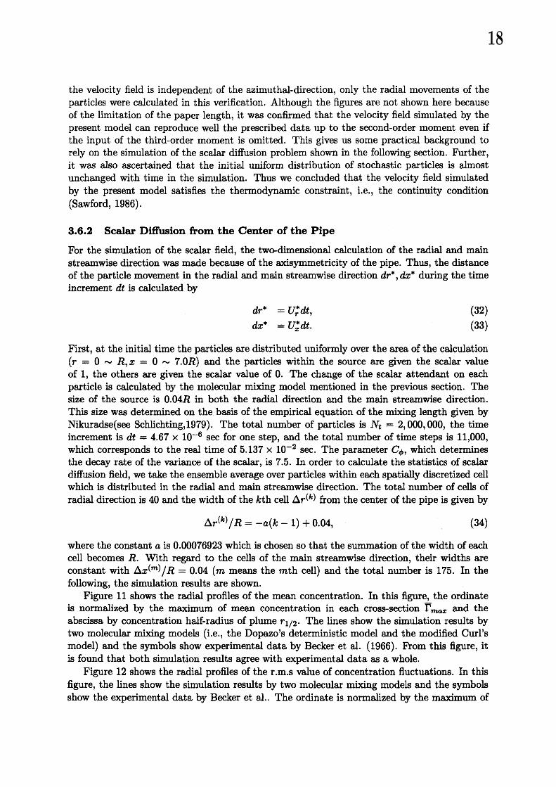
Figure 11 shows the radial profiles of the mean concentration. In this figure, the ordinateis normalized by the maximum of mean concentration in each cross-section $\overline{\Gamma}_{\max}$ and theabscissa by concentration half-radius of plume $r_{1/2}$ . The lines show the simulation results bytwo molecular mixing models (i.e., the Dopazo’s deterministic model and the modified Curl’smodel) and the symbols show experimental data by Becker et al. (1966). From this figure, itis found that both simulation results agree with experimental data as awhole.

Figure 12 shows the radial profiles of the r.m.s value of concentration fluctuations. In thisfigure, the lines show the simulation results by two molecular mixing models and the symbolsshow the experimental data by Becker et al.. The ordinate is normalized by the maximum of

18

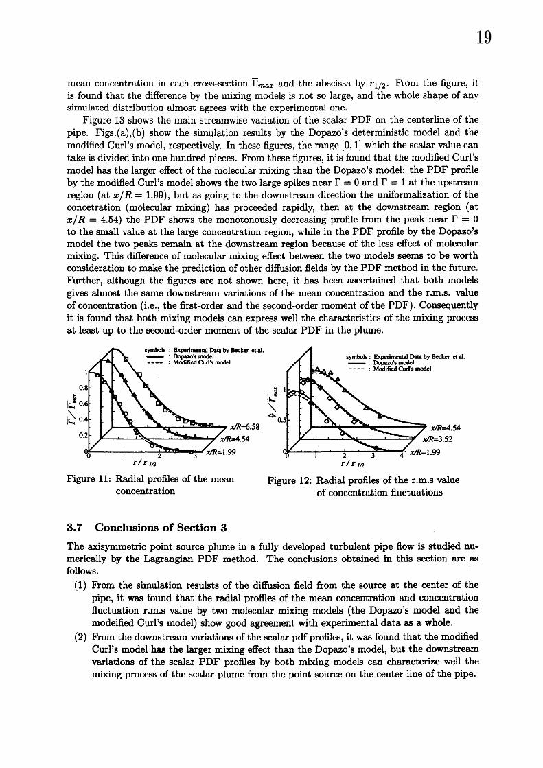
mean concentration in each cross-section $\overline{\Gamma}_{\max}$ and the abscissa by $r_{1/2}$ . From the figure, itis found that the difference by the mixing models is not so large, and the whole shape of anysimulated distribution almost agrees with the experimental one.

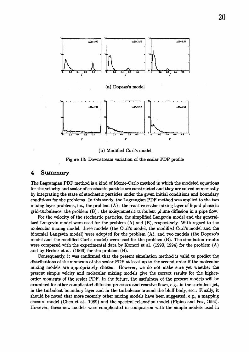
Figure 13 shows the main streamwise variation of the scalar PDF on the centerline of thepipe. Figs.(a),(b) show the simulation results by the Dopazo’s deterministic model and themodified Curl’s model, respectively. In these figures, the range $[0, 1]$ which the scalar value cantake is divided into one hundred pieces. From these figures, it is found that the modified Curl’smodel has the larger effect of the molecular mixing than the Dopazo’s model: the PDF profileby the modified Curl’s model shows the two large spikes near $\Gamma=0$ and $\Gamma=1$ at the upstreamregion (at $x/R=1.99$), but as going to the downstream direction the uniformalization of theconcetration (molecular mixing) has proceeded rapidly, then at the downstream region (at$x/R=4.54)$ the PDF shows the monotonously decreasing profile from the peak near $\Gamma=0$

to the small value at the large concentration region, while in the PDF profile by the Dopazo’smodel the two peaks remain at the downstream region because of the less effect of molecularmixing. This difference of molecular mixing effect between the two models seems to be worthconsideration to make the prediction of other diffusion fields by the PDF method in the future.Further, although the figures are not shown here, it has been ascertained that both modelsgives almost the same downstream variations of the mean concentration and the r.m.s. valueof concentration (i.e., the first-0rder and the second-0rder moment of the PDF). Consequentlyit is found that both mixing models can express well the characteristics of the mixing processat least up to the second-0rder moment of the scalar PDF in the plume.

Figure 11: Radial profiles of the mean Figure 12: Radial profiles of the r.m.s valueconcentration of concentration fluctuations

3.7 Conclusions of Section 3

The axisymmetric point source plume in afully developed turbulent pipe flow is studied nu-merically by the Lagrangian PDF method. The conclusions obtained in this section are asfollows.

(1) From the simulation resulsts of the diffusion field from the source at the center of thepipe, it was found that the radial profiles of the mean concentration and concentrationfluctuation r.m.s value by two molecular mixing models (the Dopazo’s model and themodeified Curl’s model) show good agreement with experimental data as awhole.

(2) From the downstream variations of the scalar pdf profiles, it was found that the modifiedCurl’s model has the larger mixing effect than the Dopazo’s model, but the downstreamvariations of the scalar PDF profiles by both mixing models can characterize well themixing process of the scalar plume from the point source on the center line of the pipe.

19

(a) Dopazo’s model

$\Gamma$ $\Gamma$ $\Gamma$

(b) Modified Curl’s model

Figure 13: Downstream variation of the scalar PDF profile

4Summary

The Lagrangian PDF method is akind of Monte Carlo method in which the modeled equationsfor the velocity and scalar of stochastic particle are constructed and they are solved numericallyby integrating the state of stochastic particles under the given initial conditions and boundaryconditions for the problems. In this study, the Lagrangian PDF method was applied to the twomixing layer problems, i.e., the problem (A) :the reactive-scalar mixing layer of liquid phase ingrid-turbulence; the problem (B) :the axisymmetric turbulent plume diffusion in apipe flow.

For the velocity of the stochastic particles, the simplified Langevin model and the general-ized Langevin model were used for the problem (A) and (B), respectively. With regard to themolecular mixing model, three models (the Curl’s model, the modified Curl’s model and thebinomial Langevin model) were adopted for the problem (A), and two models (the Dopazo’smodel and the modified Curl’s model) were used for the problem (B). The simulation resultswere compared with the experimental data by Komori et al. $(1993, 1994)$ for the problem (A)and by Becker et al. (1966) for the problem (B).

Consequently, it was confirmed that the present simulation method is valid to predict thedistributions of the moments of the scalar PDF at least up to the second-0rder if the molecularmixing models are appropriately chosen. However, we do not make sure yet whether thepresent simple velcity and molecular mixing models give the correct results for the higher-order moments of the scalar PDF. In the future, the usefulness of the present models will beexamined for other complicated diffusion processes and reactive flows, e.g., in the turbulent jet,in the turbulent boundary layer and in the turbulence around the bluff body, etc.. Finally, itshould be noted that more recently other mixing models have been suggested, e.g., amappingchosure model (Chen et al., 1989) and the spectral relaxation model (Pipino and Fox, 1994).However, these new models were complicated in comparison with the simple models used in

20

this study. The simplicity of the model is avery important factor for the application of themodel to the engineering problems. The use of these new models is also our future work.

Reference

Becker, H. A. ’ Rosensueing, R. E. and Gwozdz, J. R., 1966, “Turbulent Dispersion in aPipeFlow,” AIChE J., vo1.12, N0.5, pp.962-972.

Bilger, R. W., Saetran, L.R., and Krishnamoorthy, L. V., 1991, “Reaction in aScalar MixingLayer,” J. Fluid Mech., Vo1.233, pp.211-242.

Bilger, R. W., 1993, “Conditional Moment Closure for Turbulent Reacting Flow,” Phys. Fluids,A V01.5, pp. 436-444.

Corrsin, S., 1964, “The Isotropic Turbulent Mixer: Part II. Arbitrary Schmidt Number,”AIChE J., VoI.IO, pp.870-877.

Chen, H., Chen, S. and Kraichnan, R.H., 1989, “Probability Distribution of aStochasticallyAdvected Scalar Field,” Phys. Rev. Let, Vo1.63, N0.24, pp.2657-2660.

Curl, R. L., 1963, “Dispersed Phase Mixing: I. Theory and Effects in Simple Reactors,”AIChE J., Vo1.9, pp.175-181.

Dopazo, C, 1975, “Probability Density Function Approach for aTurbulent AxisymmetricHeated Jet. Centerline evolution,” Phys. Fluids, Vo1.18, pp.397-404.

Dopazo, C, 1979, “Relaxation of Initial Probability Density Functions in the TurbulentConvection of Scalar Fields,” Phys. Fluids, Vo1.22, pp.2030.

Haworth, D. C. and Pope, S. B., 1986, “A Generalized Langevin Model for Turbulent Flows,”Phys. Fluids, Vo1.29, No.2, pp.387-405.

Hinze, J.Q., 1975, “Turbulence,” 2nd ed., McGraw-Hil, New York, p.621.Hulek, T., and Lindstedt, R. P., 1995, “Transported Pdf Modelling of Nitric Oxide Conversion

in aMixing Layer,” Proceedings of the 10th Syrnposiurn on Turbulent Shear Flows,Pennsylvania State University, pp.22-7-22-12.

Janicka, J., Kolbe, W., and Kollmann, W., 1979, “Closure of the Transport Equation for theProbability Density Function of Turbulent Scalar Fields,” J. of Non-EquilibriumThermodynamics, Vo1.4, pp.47-66.

Klimenko, A., Yu., 1990, “Multicomponent Diffusion ofVarious Admixture in Turbulent Flow,”Fluid Dynamics, Vo1.25, pp.327-334.

Komori, S., Hunt, J. C. R., Kanzaki, T., and Murakami, Y., 1991, “The Effect of TurbulentMixing on the Correlation between Two Species and on Concentration Fluctuations inNon-Premixed Reacting Flows,” J. Fluid Mech., Vo1.228, pp.629-659.

Komori, S., Nagata, K., Kanzaki, T., and Murakami, Y., 1993, “Measurements of Mass Fluxin aTurbulent Liquid Flow with aChemical Reaction,” AIChE J., Vo1.39, pp.1611-1620.

Komori, S., Kanzaki, T., and Murakami, Y., 1994, “Concentration Correlation in aTurbulentMixing Layer with Chemical Reaction,” J. Chem. Eng. of Japan, Vo1.27, pp.742-748.

Leonard, A. D., Hamlen, R. C, Kerr, R. M., and Hill, J. C., 1995, “Evaluation of ClosureModels for Turbulent Reacting Flows,” Ind. &Eng. Chem. Res., Vo1.34, pp.36403652.

Laufer, J., 1954, “The Structure of Turbulence in Fully Developed Pipe Flows,” NACA Tech.,Report N0.1174.

Pipino, M., and Fox, R. O., 1994, “Reactive Mixing in aTubular Jet Reactor: AComparisonof Pdf Simulations with Experimental Data,” Chem. Eng. Sci., Vo1.49, pp.5229-5241.

Pope, S.B., 1982, “An Improved Turbulent Mixing Model,” Comb. Sci. and Tech., Vo1.28,pp.131-145.

Pope, S.B., 1985, “Pdf Method for Turbulent Reactive Flows,” Prog. Energ. &Comb. Sci.

21

$\mathrm{V}\mathrm{o}\mathrm{I}.\mathrm{I}\mathrm{I}$, pp.119-192.Pope, S.B., 1987, “Consistency Conditions for Random-walk models of Turbulent Dispersion,”

Phys. Fluids, $\mathrm{V}\mathrm{o}\mathrm{l}.30$ , N0.8, pp.2374-2379.Pope, S.B., 1994, “Lagrangian PDF Methods for Turbulent Flows,” Ann. Rev. Fluid. Mech.,

$\mathrm{V}\mathrm{o}\mathrm{l}.26$ , pp.23-63.Sakai, Y., Nakamura, I., Tsunoda, H. and Hanabusa, K., 1996, “Diffusion in Turbulent Pipe

Flow Using aStochastic Moddel,” JSME Int. J., Series $\mathrm{B}$ , $\mathrm{V}\mathrm{o}\mathrm{l}.39$ , N0.4, pp.667-675.Sawford, B.L., 1986, “Generalized random Forcing in Random-walk Turbulent Dispersion

models,” Phys. Fluids, $\mathrm{V}\mathrm{o}\mathrm{l}.29$ , No.11, pp.3582-3585.Sclichting, H., 1979, “Boundary-Layer Theory,” 7th ed., MacGraws-Hill, New York,

pp.604-606.Tennekes, H. and Lumley, J. L., 1972, “A First Course in Turbulence,” MIT Press., New York,

p.162.Toor, H. L., 1969, “Turbulent Mixing of Two Species with and without Chemical Reactions,”

$Ind$. &Eng. Chem. Rmd., $\mathrm{V}\mathrm{o}\mathrm{l}.8$, pp.655-659.Tsai, K., and Fox, R. O., 1994, “Pdf Simulation of aTurbulent Series-Parallel Reaction in an

axisymmetric Reactor,” Chem. $Eng$. Sci., $\mathrm{V}\mathrm{o}\mathrm{l}.49$ , pp.5141-5158.Valiiio, L., and Dopazo, C., 1991, “A Binomial Langevin Model for Turbulent Mixing,” Phys.

Fluids, A $\mathrm{V}\mathrm{o}\mathrm{l}.3$ , pp.30343037.

22