turbulent diffusion in the geostrophic inverse cascade - geophysical
TRANSCRIPT
J. Fluid Mech. (2002), vol. 469, pp. 13–48. c© 2002 Cambridge University Press
DOI: 10.1017/S0022112002001763 Printed in the United Kingdom
13
Turbulent diffusion in the geostrophicinverse cascade
By K. S. S M I T H, G. B O C C A L E T T I, C. C. H E N N I N G,I. M A R I N O V, C. Y. T A M, I. M. H E L D AND G. K. V A L L I S
GFDL/Princeton University, Princeton, NJ 08544, USA
(Received 28 August 2001 and in revised form 6 May 2002)
Motivated in part by the problem of large-scale lateral turbulent heat transport in theEarth’s atmosphere and oceans, and in part by the problem of turbulent transportitself, we seek to better understand the transport of a passive tracer advected byvarious types of fully developed two-dimensional turbulence. The types of turbulenceconsidered correspond to various relationships between the streamfunction and theadvected field. Each type of turbulence considered possesses two quadratic invariantsand each can develop an inverse cascade. These cascades can be modified or halted, forexample, by friction, a background vorticity gradient or a mean temperature gradient.We focus on three physically realizable cases: classical two-dimensional turbulence,surface quasi-geostrophic turbulence, and shallow-water quasi-geostrophic turbulenceat scales large compared to the radius of deformation. In each model we assume thattracer variance is maintained by a large-scale mean tracer gradient while turbulentenergy is produced at small scales via random forcing, and dissipated by lineardrag. We predict the spectral shapes, eddy scales and equilibrated energies resultingfrom the inverse cascades, and use the expected velocity and length scales to predictintegrated tracer fluxes.
When linear drag halts the cascade, the resulting diffusivities are decreasing func-tions of the drag coefficient, but with different dependences for each case. When β issignificant, we find a clear distinction between the tracer mixing scale, which dependson β but is nearly independent of drag, and the energy-containing (or jet) scale, setby a combination of the drag coefficient and β. Our predictions are tested via high-resolution spectral simulations. We find in all cases that the passive scalar is diffuseddown-gradient with a diffusion coefficient that is well-predicted from estimates ofmixing length and velocity scale obtained from turbulence phenomenology.
1. IntroductionThis paper is concerned with the problem of transport of a passive tracer in a
turbulent flow. In addition to its intrinsic interest, the problem is relevant to theissue of meridional heat transport in the Earth’s atmosphere and oceans. In mid-latitudes much of the atmospheric transport is effected by large-scale eddies that arewell-described by the quasi-geostrophic equations of motion (e.g. Pedlosky 1987). Inthe classical two-layer model of geostrophic turbulence (e.g. Rhines 1977; Salmon1980), at scales larger than the deformation radius the baroclinic streamfunction isnearly passively advected by the barotropic streamfunction, resulting in a down-scalecascade of its variance. But energy in the barotropic mode itself cascades to largescales. Since temperature is proportional to the baroclinic streamfunction, its nearly
14 K. S. Smith and others
passive advection by the barotropic flow determines the heat transport, and thisdown-gradient flux of heat in turn determines the extraction of energy from the meanflow (Larichev & Held 1995). To understand the heat transport properties of thissystem we must at least, then, understand the transport properties of a passive tracerbeing advected by a turbulent flow in which energy is cascading to larger scales, andthat is the subject of this paper.
A familiar setting in which to explore this problem is that of conventional two-dimensional turbulence (see e.g. Kraichnan & Montgomery 1980; Vallis 1993; Danilov& Gurarie 2000 for reviews). In such flows, vorticity ζ is advected by a flow defined by astreamfunction ψ linked to the vorticity, in Fourier transform space, by ζ = −|k|2ψ. Wewill find it useful to consider more general relationships between streamfunction andadvected field of the form ξ = −|k|αψ. This is not only a formal device, for a numberof physical systems can be realized by different choices of α. For example, in surfacequasi-geostrophic dynamics (e.g. Held et al. 1995), streamfunction ψ and advectedquantity ξ are related by ξ = −|k|ψ, and the equations represent the advectionof temperature along a surface bounding a constant potential vorticity interior,so providing (for example) a simple model for edge waves on the tropopause ortemperature advection near the Earth’s surface. Large-scale quasi-geostrophic flow(quasi-geostrophic dynamics at scales large compared to the radius of deformation),may be a particularly useful model for Jovian dynamics, presuming that small-scaleconvection constitutes a source of turbulent energy. The latter case correspondsto, as we will see, yet a third relationship between advected scalar and associatedstreamfunction.
The dynamics of such generalized two-dimensional turbulence was explored byPierrehumbert, Held & Swanson (1994) and Schorghofer (2000) with an emphasis onthe forward cascade properties of the flow. Our focus is on the inverse cascade and thetransport of a passive tracer by such flows. Thus, we consider fluids that are stirredat small scales by a random forcing, generating an inverse cascade, and which advecta passive tracer whose variance is maintained by a large-scale gradient. Most of thetransport of the tracer thus occurs at scales within the inverse cascade of the turbulentfluid, just as for heat transport in baroclinic turbulence. We derive general expressionsfor the spectral shape of the inverse cascade in the presence of friction, as well asestimates of the halting scale, equilibrated energy level and tracer diffusivity. Wethen test these expressions numerically for the three cases of geostrophic turbulencementioned above – conventional two-dimensional vorticity dynamics, surface quasi-geostrophic dynamics, and large-scale quasi-geostrophic dynamics – each of which hasa different relationship between streamfunction and advected scalar. In conventionaltwo-dimensional turbulence we also explore the effects of differential rotation, and wewill see that the stopping scale of the inverse cascade is not necessarily the same as themixing length of a passive scalar; we offer, and test, expressions for these two scales.
The theory presented in the paper is largely that of classical homogeneous tur-bulence, and accordingly we rely upon Kolmogorov–Kraichnan phenomenology, thepresumption of well-defined eddy scales and magnitudes, and implicitly upon theconvergence of flows to statistically steady states. Kolmogorov–Kraichnan phe-nomenology has been investigated for two-dimensional flows by many authors, andis generally found to hold best for flows that are largely free of coherent structuresand devoid of intermittency. Examples of this can be found in, e.g. Maltrud & Vallis(1991) and Sukoriansky, Galperin & Chekhlov (1999) for the inverse cascade andOetzel & Vallis (1997) and (at much higher resolution) Lindborg & Alvelius (2000)for the direct cascade. In the simulations we present, the flows are forced by small-
Turbulent diffusion in the geostrophic inverse cascade 15
scale random noise, which appears to minimize the production of coherent vorticesin the inverse cascade of standard two-dimensional turbulence. Moreover the inversecascade is, in all cases, halted before the up-scale cascading invariant reaches thedomain scale, preventing vortex condensation (Smith & Yakhot 1993). Nevertheless,in some cases investigated, coherent structures do form, and we will point out wherethese deviations from phenomenology occur.
Such phenomenology is sometimes questioned in the light of simulations of two-dimensional turbulence forced at small scales reported by Borue (1994). In thosesimulations it is found that while after a few eddy turn-around times the energyspectrum possesses a −5/3 slope, at much later times the spectrum evolves to a−3 slope, accompanied by coherent vortices in the flow. However, Borue employedan inverse hyper-viscosity (or ‘hypo’-viscosity) to absorb energy at large scales, ratherthan the more traditional and geophysically relevant linear drag. The former methodof energy dissipation has recently been shown (Danilov & Gurarie 2001) to cause thesteepening of the energy spectrum in the inverse cascade observed by Borue, whilelinear drag merely tapers the −5/3 spectrum at large scales, so long as the drag islarge enough to prevent significant energy from reaching the domain scale.
The paper is organized as follows. In § 2 we introduce the basic formalism ofgeneralized two-dimensional turbulence, and in § 3 we discuss the fundamental spectralproperties of such flows and calculate their corresponding inertial-range spectra usingKolmogorov–Kraichnan phenomenology. The dynamics of a passive tracer in aninverse cascade of generalized two-dimensional turbulence are discussed in § 4. In § 5we heuristically derive a shape for the spectrum of the inverse cascade in the presenceof drag, which in turn yields an estimate of the halting scale of the cascade. In § 6 weadd to the picture a mean vorticity gradient (the β-effect). This produces zonal jets,and we suggest expressions for both the jet scale and the eddy mixing scale. Finally,in § 7, we report on numerical tests of our scaling predictions, and conclude in § 8.An argument for cascade directions is given in Appendix A and some details of thenumerical model are relegated to Appendix B.
2. Two-dimensional flow: a generalized formalismConsider the two-dimensional advection equation for a conserved scalar field ξ
∂ξ
∂t+ J(ψ, ξ) = 0, (2.1)
where ψ is the advecting streamfunction and J(A,B) = ∂xA∂yB − ∂yA∂xB is the
Jacobian operator. The fluid velocity is given by u = k̂ × ∇ψ.In ordinary two-dimensional turbulence ξ = ∇2ψ. Restricting attention to a doubly
periodic domain, in Fourier transform space, this is equivalent to the relationshipbetween Fourier components
ξk = −k2ψk, (2.2)
where k = |k| is the isotropic two-dimensional wavenumber. More generally we canconsider the relationship between ξk and ψk discussed by Pierrehumbert et al. (1994),
ξk = −kαψk, (2.3)
where ξ will be referred to as the generalized vorticity field. The independent variablesx, y have units of length [L], and t has units of time [T ]. Therefore, in order for
16 K. S. Smith and others
(2.1) to be dimensionally balanced, ψ ∼ [L2T−1] and ξ ∼ [L2−αT−1]. Three particularvalues of α lead to geophysically relevant equations: α = 2, α = 1 and α = −2.
α = 2: Two-dimensional vorticity dynamics
If α = 2 we obtain the familiar two-dimensional Euler, or barotropic vorticityequation, with ξ = ζ and ζ ∼ [T−1]. In this paper we shall refer to these dynamics astwo-dimensional vorticity (TDV) dynamics.
α = 1: Surface quasi-geostrophic dynamics
When α = 1 we obtain surface quasi-geostrophic (SQG) dynamics (e.g. Heldet al. 1995, and references therein). These equations describe the evolution of surfacetemperature perturbations bounding a constant potential vorticity interior, within thequasi-geostrophic equations.
α = −2: Large-scale quasi-geostrophic dynamics
The case α = −2 corresponds to a rescaled shallow-water quasi-geostrophic equa-tion in the asymptotic limit of length scales large compared to the deformationscale (this system was investigated by Larichev & McWilliams 1991). We term thistype of flow large-scale quasi-geostrophic (LQG) dynamics. Consider the shallow-waterquasi-geostrophic equations
∂q
∂t+ J(ψ, q) = 0, q = (∇2 − λ2)ψ, (2.4)
where λ is the deformation wavenumber. In Fourier space the expression for thepotential vorticity q is
qk = −(k2 + λ2)ψk. (2.5)
For wavenumbers such that k � λ, we recover TDV, but when k � λ, (2.4) becomes
−λ2 ∂ψ
∂t+ J(ψ,∇2ψ) = 0. (2.6)
Because λ only appears in combination with the time derivative, we can rescale time
τ = tλ−2, (2.7)
and make the substitution of variables
ξ = ψ and Ψ = ∇2ψ (2.8)
so that (2.6) becomes
∂ξ
∂τ+ J(Ψ, ξ) = 0, Ψ = ∇2ξ. (2.9)
In Fourier space the relation between ξ and Ψ is
ξk = k−2Ψk (2.10)
which has the same form as (2.3) with α = −2.Nonlinear advection is present in all of these geophysical cases, thus turbulence
and turbulent cascades can develop. The character of the turbulence – e.g. the spectralshapes, eddy scales, cascade directions, statistical amplitudes, coherent structures andrates of turbulent development – will be distinct in each case. Some aspects of thesedistinctions were discussed by Pierrehumbert et al. (1994), who argued, for example,that the enstrophy cascade should be dominated by local strain for α < 2, and that
Turbulent diffusion in the geostrophic inverse cascade 17
local scaling predictions should break down for α > 2. Furthermore, they note thatthe inverse cascade – our primary concern in this paper – should remain local for allα < 4; the three cases discussed above fall into this category.
The fact that a single generalized formalism describes three cases of geophysicalinterest by changing the value of a single parameter provides strong motivation initself to investigate the properties of the general system. We may also regard thegeneralized turbulence formalism, however, as a shorthand with which we can derivecommon aspects of the flows without repetition.
In order to make quantitative statements about scales and energies (a necessaryprerequisite to predicting the statistics of passive tracer advection) we first considerthe Kolmogorov spectra for the generalized dynamics. Some of what follows in thenext section was derived by Pierrehumbert et al. (1994), but we include it for clarity,notation and as a reference basis for the rest of the paper.
3. Spectral properties of generalized two-dimensional flowBecause ξ is conserved on parcels, the integral over a periodic domain (or an
enclosed domain with no-normal-flow boundary conditions) of any function of ξ isconserved. Thus, there are an infinite number of invariants. However, just as for TDVflow, two quadratic invariants determine the cascade directions. From (2.1) these are
EG ≡ − 12ψξ, ZG ≡ 1
2ξ2, (3.1)
where the overline indicates a horizontal average. We will refer to EG as the gen-eralized energy, and to ZG as the generalized enstrophy. The invariants have unitsEG ∼ [L4−αT−2] and ZG ∼ [L4−2αT−2]. (Note that for LQG, T is the rescaled timefrom (2.7).) The spectra of the two quadratic invariants are connected by a simplerelationship involving scale only. To see this, we define the isotropic spectra A(k) ofthe positive definite quantity A such that
A =
∫ ∞0
A(k) dk, (3.2)
where k is the isotropic wavenumber, and A(k) is either EG(k) or ZG(k) (thus thedimensions of EG(k) ∼ [L][EG] andZG(k) ∼ [L][ZG]). The coupling relationship (2.3),together with Parseval’s theorem, implies that
ZG(k) = kαEG(k). (3.3)
Well-known arguments (Batchelor 1953) lead one to expect that, in TDV flow,energy will cascade to larger scale and enstrophy will cascade to smaller scale. Thesearguments are based on the presumption that the distribution of the spectra of eachinvariant spreads in wavenumber space. In Appendix A we extend such argumentsto the case with arbitrary α and show that, for α > 0, generalized energy cascades tolarger scale and generalized enstrophy cascades to smaller scales. For α < 0, however,it turns out that generalized energy cascades to small scales, and generalized enstrophycascades to large scale.
If there is a spectrally localized source of variance of EG and ZG, then in all theabove cases we expect there will be a transfer of generalized energy and generalizedenstrophy in opposite directions, away from the source region, just as in TDVdynamics. If frictional effects only act at some spectral distance from the source thenwe might expect inertial ranges to form between source and sink. If this is the caseone can derive the spectral slopes of these putative inertial ranges.
18 K. S. Smith and others
Between source and sink the spectral flux εE or εZ associated with the generalizedenergy or enstrophy will be constant, producing an inertial range. We assume thatover their respective inertial ranges, the local spectral density EG(k) and ZG(k) arefunctions only of the local spectral flux of EG or ZG and of the scale itself – thelocality hypothesis of Kolmogorov (1941). Thus
εA =kA(k)
TA(k)= constant, (3.4)
where A is EG or ZG and TA(k) is a local timescale. From dimensional considerations
TE(k) = [k5−αEG(k)]−1/2, (3.5a)
TZ (k) = [k5−2αZG(k)]−1/2. (3.5b)
Using the expression for the flux (3.4) we obtain
EG(k) = CEε2/3E k(α−7)/3, (3.6a)
ZG(k) = CZε2/3Z k(2α−7)/3, (3.6b)
where CE and CZ are the Kolmogorov constants for the respective cascades of EGand ZG. Because the dynamics for each type of turbulence are different, CE and CZcan depend on α. Note also that one can find the spectrum ZG(k) in the EG-range orEG(k) in the ZG-range via (3.3).
As a useful shorthand, we combine these results by writing the spectrum of ageneralized invariant as
A(k) = Cε2/3k−γ, (3.7)
where the exponent γ is
γ =
{(7− α)/3, A = EG
(7− 2α)/3, A = ZG.(3.8)
Note that as defined, γ > 1 for all cases considered in this paper. For future reference,using (3.4) and (3.7), the generalized eddy timescale is then
TA(k) = [k3γ−2A(k)]−1/2 = C−1/2ε−1/3k1−γ. (3.9)
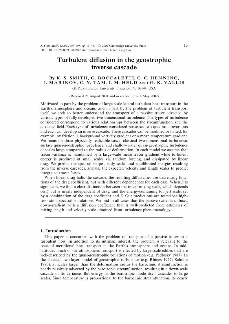
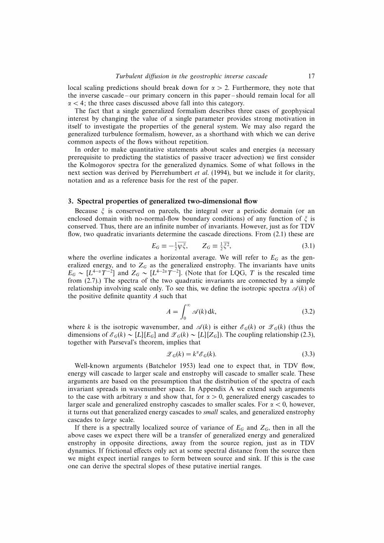
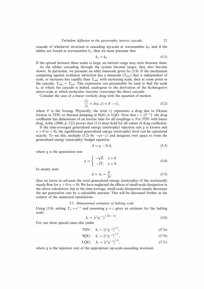
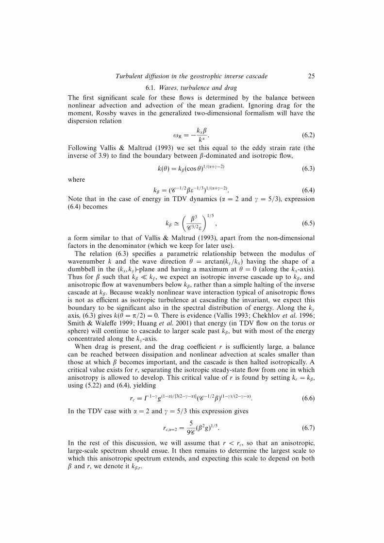
Schema of the expected cascade directions and spectral slopes for each of the threecases considered in this paper can be found in figure 1. Also noted are the dimensionalestimates of the linear drag-induced stopping scale (discussed in § 5), and the spectraof the velocity variance E for each case. The latter is necessary since r.m.s. velocitieswill be needed to predict diffusivities in § 4. In order to calculate the spectral slopeof the velocity variance one must multiply A(k), the upscale cascading invariant,by the power of k necessary to give a spectrum with dimensions [L3T−2], a powerwhich varies from case to case since A(k) has dimensions which depend on α. Onemust be careful in the LQG case, since in this case time has been re-dimensioned via(2.7). Particulars of the velocity estimates will be addressed for each case separatelyas necessary in the context of the numerical calculations discussed in § 7.
Turbulent diffusion in the geostrophic inverse cascade 19
kr~(r3/e)1/2
%G
%G =%~k–5/3
:G
:G ~k–1
%~k–3
Wavenumber
Ene
rgy
or e
ntro
phy
(a) kr~(r3/e)1/3
%G
%G ~k–2
:G
:G ~k–5/3
%~k–5/3
Wavenumber
(b)
%~k–1
kr~(r3/e)1/8
:G
:G ~k–11/3
%G
%G ~k–3
%~k–3
Wavenumber
Ene
rgy
or e
ntro
phy
(c)
%~k–5/3
Figure 1. Schematic diagram of the cascades in (a) two-dimensional vorticity dynamics, (b) surfacequasi-geostrophic dynamics, and (c) large-scale quasi-geostrophic dynamics. Each panel indicatesthe cascade directions, the spectrum of each cascading invariant in its own inertial range (EG orZG), the spectrum of the velocity variance (E), and the dimensional estimate of the scale at whichthe inverse cascade is halted by linear drag, kr . The upward arrows represent the injection of theinvariants while the downward arrows represent their dissipation.
4. Passive tracer dynamicsSuppose now that the streamfunction ψ determined by the advection equation (2.1)
and the coupling (2.3) also advects a passive tracer φ, for which the equation is
∂φ
∂t+ J(ψ, φ) = Dφ, (4.1)
where Dφ represents dissipation, presumed to occur at small scales. (In the LQG case,the streamfunction advecting the tracer is the QG streamfunction ψ, which determinesthe velocities, rather than the redefined streamfunction of (2.8).) The tracer variance
P ≡ 12φ2 (4.2)
is a conserved quantity of the tracer field in the absence of dissipation. In the inertialrange of A – some conserved quantity of the flow field – the spectral flux χ of tracervariance is
χ =kP(k)
TE(k)= constant, (4.3)
where P(k) is the spectrum of the tracer variance and TE(k) is the timescale associatedwith the kinetic energy in the inertial range of A. In general there is only one spectrally
20 K. S. Smith and others
local timescale available, namely (3.9). In this case the tracer variance spectrum is
P(k) =Kχε−1/3k−γ, (4.4)
where K is the Kolmogorov constant for the tracer. In general, then, the tracervariance follows the same power law as the spectrum of the advecting flow invariant,in that invariant’s inertial range. For example, in the case α = 2 (TDV), tracer variancehas the slope −5/3 in the energy inertial range, and slope −1 in the enstrophy inertialrange.
When LQG describes the dynamics, however, these predictions should only holdif the tracer is advected by the redefined streamfunction. This is not the relevantphysical situation. The variance of the tracer as given by (4.1) requires that we specifythe timescale TE(k) in terms of physical scales, which re-introduces the deformationscale into the calculation. The up-scale cascading invariant is then associated withthe available potential energy (APE) and the direct cascading invariant is the kineticenergy (KE). The latter has a spectral slope of k−5/3 in the inertial range of the APE,yielding an expected tracer variance spectral slope of k−5/3 as well.
Suppose now that tracer variance is generated by the presence of a fixed large-scalemeridional gradient and absorbed by small-scale dissipation. Specifically, we consider
∂φ
∂t+ J(ψ, φ) + θν = Dφ, (4.5)
where ν = ∂ψ/∂x is the meridional velocity of the advecting flow and θ ≡ ∂φ̄/∂y isthe mean tracer gradient. Since (4.5) is linear in φ, we can rescale the equation suchthat θ = 1. Multiplying (4.5) by −φ and averaging over space yields
dP
dt= φν − φDφ, (4.6)
where P is the tracer variance of (4.2). The meridional flux of tracer is the explicitsource of variance in the tracer field, and can be written
φν = −D, (4.7)
where D is the diffusivity, which has dimensions [L2T−1] = [VL]. If the advectingmeridional velocity field is sharply peaked at some scale k0 and has a r.m.s. valueVrms, then a standard downgradient mixing hypothesis (e.g. Tennekes & Lumley 1994,chap. 8) yields an expected diffusivity
D ' Vrmsk−10 . (4.8)
One can make a crude estimate of the tracer flux spectrum by decomposing theleft-hand side of (4.7) and estimating the two fields separately, yielding
D(k) ∼ E1/2(k)P1/2(k), (4.9)
We shall derive specific diffusivity estimates for each of our cases and test theiraccuracy numerically. In order to do so, however, we must first derive estimates fork0 and Vrms.
5. Cascade reduction by linear dragAn inverse cascade will be diminished or halted when the up-scale-cascading
invariant either reaches the domain scale, or the scale at which some competingprocess such as friction dominates nonlinear advection. If some mechanism halts the
Turbulent diffusion in the geostrophic inverse cascade 21
cascade of whichever invariant is cascading up-scale at wavenumber k0, and if theeddies are forced at wavenumber kf , then we must presume that
kf > k0. (5.1)
If the spread between these scales is large, an inertial range may exist between them.As the eddies cascading through the system become larger, they also become
slower. In particular, we presume an eddy timescale given by (3.9). If the mechanismcompeting against nonlinear advection has a timescale (Thalt) that is independent ofscale, or increases less rapidly than Teddy with increasing scale, then at some point inthe cascade, Teddy ∼ Thalt. This expression can presumably be used to find the scalek0 at which the cascade is halted, analogous to the derivation of the Kolmogorovmicro-scale at which molecular viscosity overcomes the direct cascade.
Consider the case of a linear vorticity drag with the equation of motion
∂ξ
∂t+ J(ψ, ξ) = F − rξ, (5.2)
where F is the forcing. Physically, the term rξ represents a drag due to Ekmanfriction in TDV, or thermal damping in SQG or LQG. Note that r ∼ [T−1]: the dragcoefficient has dimensions of an inverse time for all couplings α. For TDV with lineardrag, Arbic (2000, p. 122) proves that (5.1) must hold for all values of drag coefficient.
If the time-averaged generalized energy (enstrophy) injection rate g is known andα > 0 (α < 0), the equilibrated generalized energy (enstrophy) level can be calculatedexactly. To see this, multiply (5.2) by −ψ(−ξ) and integrate over space to form thegeneralized energy (enstrophy) budget equation
A = g − 2rA, (5.3)
where g is the generation rate
g =
{ −ψF, α > 0
−ξF, α < 0.(5.4)
In steady state
A = Ar =g
2r, (5.5)
thus we know in advance the total generalized energy (enstrophy) of the statisticallysteady flow for α > 0 (α < 0). We have neglected the effects of small-scale dissipation inthe above calculation, but in the time-average, small-scale dissipation simply decreasesthe net generation rate by a calculable amount. This will be discussed further in thecontext of the numerical simulations.
5.1. Dimensional estimates of halting scale
Using (3.9), setting TA = r−1 and assuming g = ε gives an estimate for the haltingscale:
kr ∼ (r3g−1)1/[3(γ−1)]
. (5.6)
For our three special cases this yields
TDV: kr ∼ (r3g−1)1/2
, (5.7a)
SQG: kr ∼ (r3g−1)1/3
, (5.7b)
LQG: kr ∼ (r3g−1)1/8
, (5.7c)
where g is the injection rate of the appropriate up-scale-cascading invariant.
22 K. S. Smith and others
The expression (5.6) is demanded by dimensional consistency, and so gives noindication of the value of any numerical prefactor. One simple way to derive such aprefactor is to note that the integral of the energy spectrum (3.7) must be consistentwith the total energy as given by (5.5). That is,∫ ∞
kr
Cε2/3k−γ dk =g
2r, (5.8)
where we have assumed that the energy content in the larger scales (k < kr) isnegligible. For γ > 1 this gives
kr ≈(
2Cγ − 1
)1/(γ−1)(r3g−1
)1/[3(γ−1)], (5.9)
which is identical to (5.6), except for the numerical coefficient involving theKolmogorov constant. For TDV, this gives
kr ≈ (3C)3/2(r3g−1
)1/2. (5.10)
Danilov & Gurarie (2001) independently proposed an identical scaling. This coefficientis accurate only to the extent that the energy falls off very rapidly for wavenumberssmaller than kr .
5.2. Spectral shapes
By making one additional assumption, we can derive an expression for the spectralshape that is putatively valid in the inertial range and in the range where frictionbegins to dominate. The peak of this theoretical spectrum, derived in a manner similarto that of Leith (1967) and Lilly (1972), yields a better estimate for the stopping-scaleprefactor than (5.9). However, we only expect the theory to be relevant in parameterregimes such that the underlying inertial range is present and free of intermittency,and make no claim that the derived spectral shape is universal.
The spectral budget equation for generalized energy (enstrophy) in mode k forα > 0 (α < 0) is
∂Ak
∂t= εk − 2rAk + gδ(k − kf), (5.11)
where Ak = |ψk|2/2 (or Re[ξ∗kψk]/2), εk is the transfer rate at k arising from the realpart of the product of −ψ∗k and the spectral Jacobian term, and g is the generalizedenergy (enstrophy) injection, localized at isotropic wavenumber kf . We assume asteady state, so that the time derivative vanishes, and isotropy so that k can bereplaced by k. If the source term is at some high wavenumber kf � kr then we mayexpect an inverse cascade initially unfettered by friction. At smaller wavenumbers,the drag will remove energy from the flow, and, without further approximation, thespectral transfer is governed by the budget equation
dε
dk= 2rA(k). (5.12)
That is, the energy flux is reduced by the frictional loss.We now assume that the spectrum (3.7) can be substituted forA(k), but let ε = ε(k)
therein. This is a perturbative solution for small drag-induced deviations from theinertial-range flux. Thus we expect the approximation to be valid in the spectralregions where drag is small and up to the scales where it begins to dominate, but not
Turbulent diffusion in the geostrophic inverse cascade 23
at the frictionally dominated, largest scales. In this approximation (5.12) becomes
dε
dk= 2rCε2/3k−γ, (5.13)
which readily yields
ε(k) =
[2C
3(1− γ)rk1−γ + c
]3
, (5.14)
where c is the integration constant. The transfer rate must be equal to the generationrate at the forcing scale, i.e.
ε(kf) = g, (5.15)
which we use to solve for the integration constant in (5.14). Using the solution for c,the flux is
ε(k) = g[1− (kc/k)
γ−1 + (kc/kf)γ−1]3, (5.16)
where
kc =
[2C
3(γ − 1)
]1/(γ−1)
(r3g−1)1/[3(γ−1)]. (5.17)
Substituting this into (3.7) gives us an estimate for the spectrum of the invariant inthe presence of linear drag:
A(k) = Cg2/3k−γ[1− (kc/k)(γ−1) + (kc/kf)
γ−1]2. (5.18)
For TDV, the expression (5.18) in the limit kf → ∞ was derived by Lilly (1972). Thereader may verify that the expression for A(k) satisfies∫ ∞
kc
A(k) dk =g
2r(5.19)
exactly.For kf � kc, the third term in brackets is small and can be neglected (but we shall
retain it in our predictions for the simulated spectra). For wavenumbers k � kc, thesecond term in square brackets in (5.18) is also negligible and the spectrum reducesto (3.7). For sufficiently small wavenumbers, ε(k) given by (5.16) is not positive. Thecritical wavenumber at which the spectral flux vanishes is k = kc (assuming kf →∞),where kc is given by (5.17). It is unphysical for A(k) to vanish identically at somefinite k. The weakness of this derivation is just the use of the inertial-range spectrum(3.7) in (5.12), an assumption we expect to be valid only if frictional effects are smallperturbations on the inertial flow, as mentioned above.
The predicted spectral shapes for the three cases we consider here are (assumingkf →∞)
TDV: E(k) = Cg2/3k−5/3[1− (kc/k)2/3]2, kc = C3/2(r3g−1)1/2, (5.20a)
SQG: E(k) = Cg2/3k−2[1− (kc/k)]2, kc = (2C/3)(r3g−1)1/3, (5.20b)
LQG: Z(k) = Cg2/3k−11/3[1− (kc/k)8/3]2, kc = (C/4)3/8(r3g−1)1/8, (5.20c)
where in each case the spectrum is valid for all k > kc, and C and g are theKolmogorov constant and injection rate, respectively, for the particular dynamics athand.
A quantitative estimate of the drag-induced halting scale can be made by calculating
24 K. S. Smith and others
the location of the peak wavenumber k0 = kr by setting
dA(k)
dk
∣∣∣∣k=kr
= 0. (5.21)
This yields
kr = Γ (r3g−1)1/[3(γ−1)], Γ =
[2C(3γ − 2)
3γ(γ − 1)
]1/(γ−1)
. (5.22)
For our three cases, the drag-induced stopping scales expected are
TDV: kr = (9C/5)3/2(r3g−1)1/2, (5.23a)
SQG: kr = (4C/3)(r3g−1)1/3, (5.23b)
LQG: kr = (27C/44)3/8(r3g−1)1/8. (5.23c)
As in (5.10), the prefactor Γ in each case is not necessarily an order-unity quantity.In the case of energy in TDV turbulence, for example, using the estimate C = 5.8(Maltrud & Vallis 1991) yields Γ = (9C/5)3/2 = 33.7. Using (5.10) gives 72.6, thelarger number being consistent with the assumption that energy is strictly zero forwavenumbers smaller than kr . Our numerical results (discussed in § 7) are consistentwith these estimates; that is, the strictly dimensional estimate kr = (r3/g)1/2 is morethan an order of magnitude smaller than the actual wavenumber at which thecascade is halted. The large value of Γ indicates that, in the presence of drag, TDVturbulence is more inefficient at moving energy to larger scales than one might expectfrom dimensional estimates alone.
6. Mean vorticity gradients: the β-effectIn two-dimensional vorticity dynamics, a meridional gradient of planetary vorticity
may be represented by the β-effect. In SQG, a meridional gradient of temperature givesrise to a similar term in the equation of motion. Including such effects in (5.2), we write
∂ξ
∂t+ J(ψ, ξ) + β
∂ψ
∂x= F − rξ, (6.1)
where we use the symbol β for the constant mean gradient of ξ with unitsβ ∼ [L1−αT−1]. Because β introduces anisotropy into the dynamics (Rhines 1975;Vallis & Maltrud 1993), the halting scale, if present, will be anisotropic as well. How-ever, the dual presence of β and r introduces complexities to the dynamics which,even for TDV, have only recently come to be appreciated (Chekhlov et al. 1996; Man-froi & Young 1999; Smith & Waleffe 1999; Huang, Galperin & Sukoriansky 2001;Galperin, Sukoriansky & Huang 2001; Danilov & Gryanik 2001). The mean vorticitygradient admits a possible tri-partite balance in the equation of motion betweennonlinear advection, advection of the mean gradient (and thereby possible wavepropagation) and dissipation.
We direct the discussion here to the two cases with α > 0: TDV and SQG. The β-term as defined in (6.1) physically represents the Coriolis gradient in TDV, and a meantemperature gradient in SQG, but has no obvious physical interpretation for LQG†.† Keeping the same definition of β as in TDV, we obtain a term of the form β∂ξ/∂x added
to the left-hand side of (2.9). The dispersion relation is the same as that for equivalent barotropicRossby waves at large scales, namely ωR,LQG = −kxβ/λ2. The frequency goes linearly to zero ratherthan diverging at large scale, hence it is not clear that β can halt the cascade in this case.
Turbulent diffusion in the geostrophic inverse cascade 25
6.1. Waves, turbulence and drag
The first significant scale for these flows is determined by the balance betweennonlinear advection and advection of the mean gradient. Ignoring drag for themoment, Rossby waves in the generalized two-dimensional formalism will have thedispersion relation
ωR = −kxβkα. (6.2)
Following Vallis & Maltrud (1993) we set this equal to the eddy strain rate (theinverse of 3.9) to find the boundary between β-dominated and isotropic flow,
k(θ) = kβ(cos θ)1/(α+γ−2) (6.3)
where
kβ = (C−1/2βε−1/3)1/(α+γ−2). (6.4)
Note that in the case of energy in TDV dynamics (α = 2 and γ = 5/3), expression(6.4) becomes
kβ '(
β3
C3/2ε
)1/5
, (6.5)
a form similar to that of Vallis & Maltrud (1993), apart from the non-dimensionalfactors in the denominator (which we keep for later use).
The relation (6.3) specifies a parametric relationship between the modulus ofwavenumber k and the wave direction θ = arctan(ky/kx) having the shape of adumbbell in the (kx, ky)-plane and having a maximum at θ = 0 (along the kx-axis).Thus for β such that kβ � kf , we expect an isotropic inverse cascade up to kβ , andanisotropic flow at wavenumbers below kβ , rather than a simple halting of the inversecascade at kβ . Because weakly nonlinear wave interaction typical of anisotropic flowsis not as efficient as isotropic turbulence at cascading the invariant, we expect thisboundary to be significant also in the spectral distribution of energy. Along the kyaxis, (6.3) gives k(θ = π/2) = 0. There is evidence (Vallis 1993; Chekhlov et al. 1996;Smith & Waleffe 1999; Huang et al. 2001) that energy (in TDV flow on the torus orsphere) will continue to cascade to larger scale past kβ , but with most of the energyconcentrated along the ky-axis.
When drag is present, and the drag coefficient r is sufficiently large, a balancecan be reached between dissipation and nonlinear advection at scales smaller thanthose at which β becomes important, and the cascade is then halted isotropically. Acritical value exists for r, separating the isotropic steady-state flow from one in whichanisotropy is allowed to develop. This critical value of r is found by setting kr = kβ ,using (5.22) and (6.4), yielding
rc = Γ 1−γg(1−α)/[3(2−γ−α)](C−1/2β)(1−γ)/(2−γ−α). (6.6)
In the TDV case with α = 2 and γ = 5/3 this expression gives
rc,α=2 =5
9C (β2g)1/5. (6.7)
In the rest of this discussion, we will assume that r < rc, so that an anisotropic,large-scale spectrum should ensue. It then remains to determine the largest scale towhich this anisotropic spectrum extends, and expecting this scale to depend on bothβ and r, we denote it kβ,r .
26 K. S. Smith and others
6.2. Estimates of the halting scale with β and drag present
For clarity of presentation we focus on TDV, and then discuss how it may be adaptedto generalized two-dimensional turbulence. In the small-drag limit (r � rc) we seekan estimate for the halting scale kβ,r , that is for the scale at which the maximumenergy is found. Because in anisotropic turbulence most of the energy goes into zonaljets it is not surprising that this estimate will be particularly apt as an estimatefor the separation scale of the jets themselves. Our argument has two components:(i) the forcing and dissipation set the r.m.s. velocity; (ii) using this in conjunctionwith the β-effect provides an estimate of the halting scale. We shall see that despite thejet scale being the most energetic scale, it is the inviscid scale (6.4) that characterizesthe meridional transport of passive tracer.
If one assumes that, at scales where β is important but where drag is not yetsignificant (kβ,r < k < kβ), the spectral slope is a function only of β and wavenumber,then dimensional analysis leads to the expression
Eβ(k) = Cββ2k−5, (6.8)
as pointed out by Rhines (1975). Obviously, though, the spectrum cannot be isotropic,since it is derived specifically in the region where anisotropy is present. Our simula-tions, as well as those of Galperin et al. (2001) and others cited above, demonstratethat at scales kβ,r < k < kβ , energy is concentrated along the kx = 0 axis, but doesroughly follow a k−5 power law. Chekhlov et al. (1996) point out that energy continuesto follow a k−5/3 power law for all wavenumbers kβ,r < k < kβ with kx 6= 0, but thatimplies that modes with kx 6= 0 contribute negligibly to the total spectrum at largescale.
Chekhlov et al. (1996) and Smith & Waleffe (1999) discuss the subtleties of thetransfer from the two-dimensional isotropic cascade to the one-dimensional ‘cascade’along the zonal axis. If the energy is concentrated on the kx = 0 axis, precisely wherethe β-term in (6.1) vanishes, then the dependence on β of (6.8) is unexpected. Adependence on β might arise if resonant nonlinear triad interactions among Rossbywaves were responsible for the transfer to zonal flow, but these are unable to transferenergy from isotropic two-dimensional motions to modes with kx = 0. Newell (1969)suggests that quartic resonances or near resonances could explain these transfers, thusmaintaining a β-dependence in the spectrum. Danilov & Gryanik (2001) point outthat in fact the zonal energy is not distributed as a uniform spectrum, but rather as aseries of peaks whose amplitudes increase roughly like k−5, and provide a preliminaryexplanation for the observed wavenumber dependence. Given all of the above, wewill take the appearance of such a −5 spectrum (or wavenumber dependence ofthe spectral peaks) as an empirical observation with a rather weak theoretical orphenomenological justification.
Thus, we will suppose an isotropic k−5/3 spectra at scales kβ < k < kf , an anisotropick−5 spectral distribution, with most energy concentrated along the zonal axis, at scaleskβ,r < k < kβ , and negligible energy at k < kβ,r . That is,
E(k) 'Cε2/3k−5/3, kβ < k < kf
Cββ2k−5, kβ,r < k < kβ, kx = 0
0, k < kβ,r.
(6.9)
We use this phenomenological picture to determine kβ,r . Note that even in thepresence of β, (5.3) remains valid, so that the total energy is E = g/2r. This constraint
Turbulent diffusion in the geostrophic inverse cascade 27
determines the lowest wavenumber which the inverse cascade may reach, just as in(5.9). Specifically, using (6.9) we set∫ ∞
kβ,r
E(k) dk ' g
2r. (6.10)
Because the spectra are so steep in the Rossby wave regime, the integral is dominatedby contributions from its peak at the low-wavenumber end, giving
kβ,r '(Cββ2r
2g
)1/4
. (6.11)
A simpler derivation results if we begin with the familiar expression for the stoppingscale (Rhines 1975)
kβ,r = (βU−1rms)
1/2. (6.12)
But from (5.5) Urms = (g/r)1/2 (where we have also assumed that Urms � Vrms), andsubstituting this into (6.12) we obtain (6.11), albeit without the numerical constant.Note that (6.12) is an estimate for a marginally barotropically unstable jet.
Manfroi & Young (1999) predict a jet-separation scale proportional to r−1/3, orequivalently, kβ,r ∝ r1/3. Distinguishing between r−1/3 and r−1/4 (the latter from our(6.11)) is difficult numerically due both to the small difference in exponent and to theslow equilibration of the flow in this parameter regime.
We can formally derive an anisotropic wave spectrum in the general case assuminga balance between the wave frequency (6.2) and the inverse of the eddy timescale of(3.9). The wave spectrum in this case is
Aβ(k) = Cββ2k4−2α−3γ, (6.13)
which reduces to (6.8) in the inverse cascade of TDV. In SQG we find a k−4 spectrumin the Rossby wave regime, also significantly steeper than the isotropic spectrum ofk−2 relevant in that case.
The result analogous to (6.11) for the general case is
kβ,r '[
2Cββ2r
(2α+ 3γ − 5)g
]1/(2α+3γ−5)
. (6.14)
The simple argument using the analogue of (6.12) is not always possible in thegeneralized case, because the integral constraint corresponding to (5.3) does notalways give a value for the r.m.s. velocity. For example, in SQG, the generalizedenergy E = ψξ/2 is not a velocity squared. Rather, it is the generalized enstrophythat has units of velocity squared, but its value is not constrained solely by the forcingand the drag.
Which of the scales (6.5) and (6.11) (or (6.4) and (6.14) in the general case) is relevantfor the meridional transport of a passive tracer? The scale (6.11) determines a jetscale, with vanishing meridional velocity. Bartello & Holloway (1991) demonstratethat at the jet scale, zonal advection so dominates meridional advection that littlemeridional mixing occurs. We thus expect the scale (6.5), the largest scale of isotropicturbulence, to act as a mixing length, and explore this further in § 7. Held & Larichev(1996) utilized the scaling (6.5), without the numerical prefactor, as a mixing lengthin their theory for turbulent quasi-geostrophic heat fluxes.
28 K. S. Smith and others
7. Numerical examinations of diffusivity scalingsWe now describe sets of numerical simulations designed to test the diffusivity
predictions for TDV, SQG and LQG with linear drag. We also test TDV with lineardrag and β. Mixing lengths for each case have been derived in the previous twosections, but velocity scales have not – both are required for estimates of diffusivitygiven by (4.8). It is difficult to generalize the calculation of velocity variance amongthe various cases, so we consider this detail, and the predictions for the diffusivitiesthemselves, in the context of each case separately.
All simulations were performed using a two-dimensional de-aliased spectral modelwith 5122 equivalent horizontal gridpoints (kmax/kmin = 255). A leap-frog timestep isused to advance the solution, and a weak Robert filter suppresses the computationalmode. In each case, a passive tracer is advected with the calculated flow. The flow isforced with an isotropic forcing at high wavenumber, typically about kf/kmin = 160.The magnitude of the generation rate is fixed at g = 1, less an amount due tosmall-scale dissipation (see Appendix B for details of the forcing function).
Small-scale variance in both the generalized vorticity field (i.e. enstrophy) and inthe tracer field are dissipated with a highly scale-selective exponential cutoff filter((B 9) and (B 10)) with vanishing dissipation below a cutoff wavenumber kcut. For allsimulations presented here, kcut/kmin = 165 for the advecting flow and kcut/kmin = 1for the tracer. The exponent s in (B 9) is s = 8 for the advecting flow and s = 2 forthe tracer. For the advecting flow, kcut is just larger than the forcing scale and is thescale at which we begin to allow small-scale dissipation – traditional hyperviscosity, bycontrast, dissipates at all scales. The dissipation level does not become significant untilnear the maximum wavenumber in the computational domain. Thus, while we focushere on maintaining as wide an inverse cascade range as possible, we have alloweda reasonable direct cascade for wavenumbers k > kf . The small-scale dissipation,despite its presence only at k > kf , removes some of the up-scale-cascading invariant.We calculate this loss and use it to define a geff < g = 1 (geff ' 0.5 for all thesimulations – see Appendix B).
In each of the following sections, we state values as non-dimensionalized using alength given by the inverse forcing scale L = k−1
f and a time given by a combinationof the generation rate g and forcing scale. The former has units
g ∼ [L3(γ−1)T−3],
so that a non-dimensional measure of the time is
T = [gk3(γ−1)f ]−1/3. (7.1)
All values with a ∗ superscript have been non-dimensionalized by these scales.For each dynamical case considered, a series of simulations was performed.
Each simulation described is run for several eddy turnover times after a statisticallysteady state is achieved; averages are taken over the equilibrated phase of a givenrun. Each simulation was performed with a different drag coefficient, the values ofwhich were chosen such that the halting scales were large compared to the forcingscale, but not too close to the domain scale.
7.1. Two-dimensional vorticity flow with linear drag
We begin with the straightforward case of two-dimensional vorticity dynamics dis-sipated by linear drag, namely equations (5.2) and (2.3) with α = 2. In this case Ecascades up-scale with spectral slope γ = 5/3. Five simulations were performed in
Turbulent diffusion in the geostrophic inverse cascade 29
which the drag was set to
r∗ = r(gk2f)−1/3 = (0.86, 1.5, 2.4, 3.7, 6.0)× 10−2.
We predict a spectral shape given by (5.20a) and a spectral peak given by (5.23a).Since the total energy, according to (5.5), is E = g/2r = (U2
rms + V 2rms)/2 ' V 2
rms
(assuming isotropy), the integrated (r.m.s.) meridional velocity Vrms is
Vrms =( g
2r
)1/2
. (7.2)
Using (4.8), (5.23a) and (7.2), we estimate the eddy diffusivity, or integrated tracerflux, to be
D '[(
5
9C)3
1
2
]1/2
gr−2. (7.3)
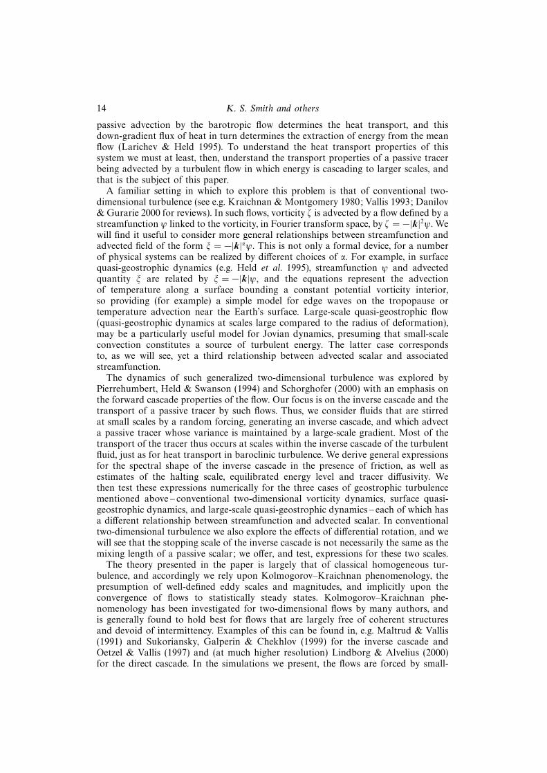
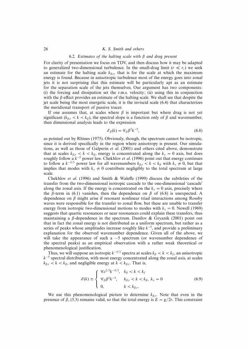
We use C = 6 in numerical estimates.Figure 2 shows the spectra of the energy, tracer variance and tracer flux, as well as
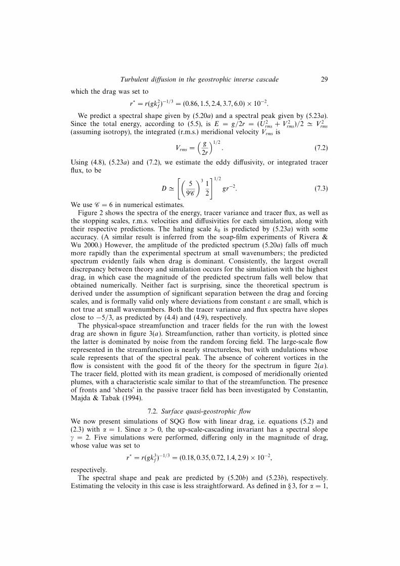
the stopping scales, r.m.s. velocities and diffusivities for each simulation, along withtheir respective predictions. The halting scale k0 is predicted by (5.23a) with someaccuracy. (A similar result is inferred from the soap-film experiments of Rivera &Wu 2000.) However, the amplitude of the predicted spectrum (5.20a) falls off muchmore rapidly than the experimental spectrum at small wavenumbers; the predictedspectrum evidently fails when drag is dominant. Consistently, the largest overalldiscrepancy between theory and simulation occurs for the simulation with the highestdrag, in which case the magnitude of the predicted spectrum falls well below thatobtained numerically. Neither fact is surprising, since the theoretical spectrum isderived under the assumption of significant separation between the drag and forcingscales, and is formally valid only where deviations from constant ε are small, which isnot true at small wavenumbers. Both the tracer variance and flux spectra have slopesclose to −5/3, as predicted by (4.4) and (4.9), respectively.
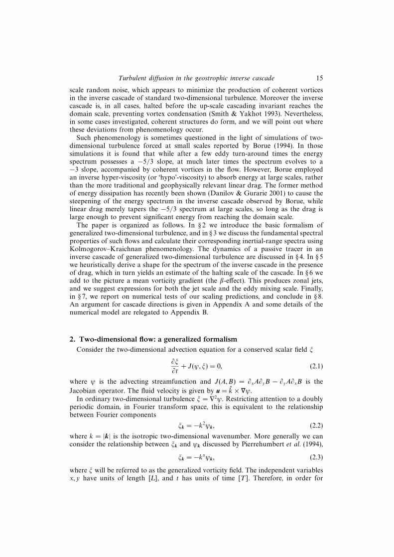
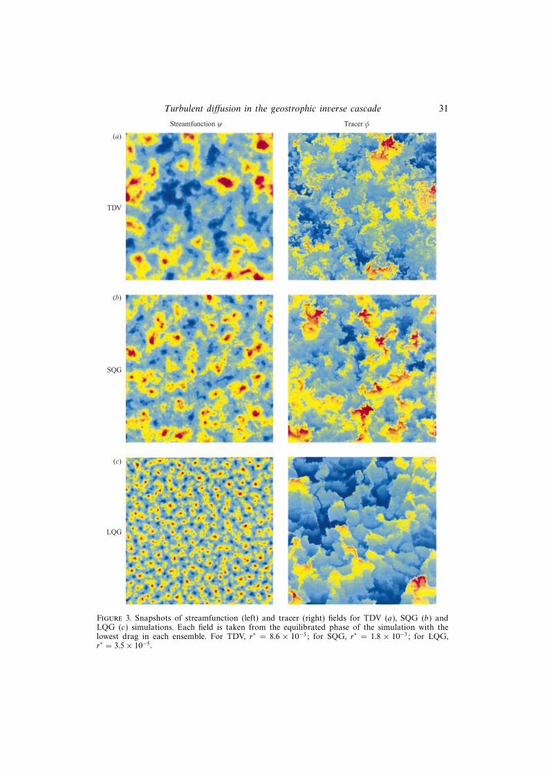
The physical-space streamfunction and tracer fields for the run with the lowestdrag are shown in figure 3(a). Streamfunction, rather than vorticity, is plotted sincethe latter is dominated by noise from the random forcing field. The large-scale flowrepresented in the streamfunction is nearly structureless, but with undulations whosescale represents that of the spectral peak. The absence of coherent vortices in theflow is consistent with the good fit of the theory for the spectrum in figure 2(a).The tracer field, plotted with its mean gradient, is composed of meridionally orientedplumes, with a characteristic scale similar to that of the streamfunction. The presenceof fronts and ‘sheets’ in the passive tracer field has been investigated by Constantin,Majda & Tabak (1994).
7.2. Surface quasi-geostrophic flow
We now present simulations of SQG flow with linear drag, i.e. equations (5.2) and(2.3) with α = 1. Since α > 0, the up-scale-cascading invariant has a spectral slopeγ = 2. Five simulations were performed, differing only in the magnitude of drag,whose value was set to
r∗ = r(gk3f)−1/3 = (0.18, 0.35, 0.72, 1.4, 2.9)× 10−2,
respectively.The spectral shape and peak are predicted by (5.20b) and (5.23b), respectively.
Estimating the velocity in this case is less straightforward. As defined in § 3, for α = 1,

30 K. S. Smith and others
103
102
101
100
10–2 10–1 100
k /kf
(a)
10–2 10–1 100
k /kf
(b)
–5/3
10–2
10–3
10–4
10–5
10–6
P(k
)
E(k
)/(g
kf–5
/2)2/
3
(c) (d)
100
10–1
10–2
10–2 10–1
r /(g k f2)1/3
k0/k
f
Vrm
s/(g
kf–1
)1/3
101
100
10–2 10–1
r /(g k f2)1/3
(e) ( f )
10–2 10–1
r /(g k f2)1/3
10–2 10–1 100
k /kf
103
102
101
D/(
g k
f–4 )
1/3
104
102
101
100
D(k
)/(g
kf–7
)1/3
103 –5/3
Figure 2. Equilibrated statistics for five simulations of TDV dynamics which differ only in thevalue of the drag coefficient. Values of drag used are r∗ = (0.86, 1.5, 2.4, 3.7, 6.0) × 10−2 and theeffective generation rates are geff = 0.57, 0.59, 0.61, 0.64, 0.69. All statistics are non-dimensionalizedby the timescale (7.1) and the length scale k−1
f . Panels show (a) energy spectra as a function of totalwavenumber (solid) and theoretical predictions (dashed) for each simulation; (b) tracer variancespectra as a function of total wavenumber for each simulation; (c) peaks of energy spectra (stars)and theoretical prediction (solid) vs. drag; (d ) r.m.s. meridional eddy velocity (stars) and theoreticalprediction (solid) vs. drag; (e) tracer flux spectra (the spectra of −ν ′φ′) as a function of totalwavenumber for each simulation; ( f ) integrated tracer flux −ν ′φ′ (stars) and theoretical predictionfor the diffusivity (solid) vs. drag. Theoretical predictions are discussed in § 7.1. In this case, thehalting scale k0 is compared to the drag scale kr .
Turbulent diffusion in the geostrophic inverse cascade 31
TDV
(a)
Streamfunction w
SQG
(b)
LQG
(c)
Tracer φ
Figure 3. Snapshots of streamfunction (left) and tracer (right) fields for TDV (a), SQG (b) andLQG (c) simulations. Each field is taken from the equilibrated phase of the simulation with thelowest drag in each ensemble. For TDV, r∗ = 8.6 × 10⁻³; for SQG, r∗ = 1.8 × 10⁻³; for LQG,r∗ = 3.5× 10⁻⁵.
32 K. S. Smith and others
the invariants of the flow have units E ∼ [L3T−2] and Z ∼ [L2T−2], thus in thiscase Z has the dimensions of energy (physically it is the temperature variance, oravailable potential energy). In SQG then, the r.m.s. velocity of the flow is relatedto the generalized enstrophy as Z = V 2
rms (assuming isotropy). Ignoring drag for themoment, in the inverse cascade range Z has the spectrum
Z(k) = CEε2/3E k−1. (7.4)
The integral of this spectrum diverges logarithmically, and we must explicitly includethe forcing scale
Z '∫ kf
kc
Z(k) dk, (7.5)
where kc is as given by (5.20b). We thus obtain our estimate of the r.m.s. meridionalvelocity scale
Vrms = [CEg2/3 ln(kf/kc)]1/2, (7.6)
where we have taken g = εE .
Using (4.8), (5.23b) and (7.6), we estimate the eddy diffusivity, or integrated tracerflux, to be
D ' (g2/3r−1)
[9
16CE ln(kf/kc)
]1/2
. (7.7)
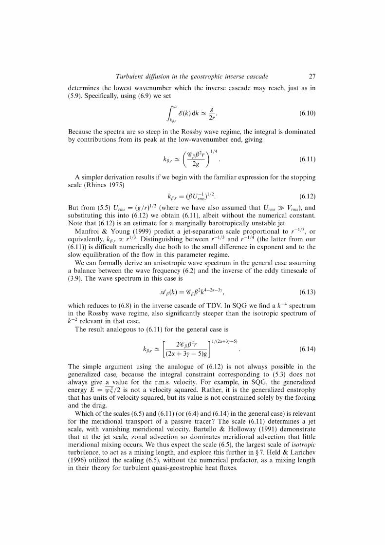
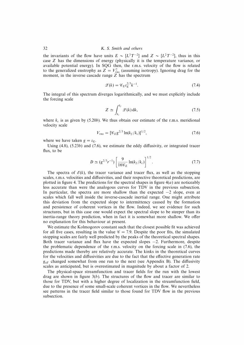
The spectra of E(k), the tracer variance and tracer flux, as well as the stoppingscales, r.m.s. velocities and diffusivities, and their respective theoretical predictions, areplotted in figure 4. The predictions for the spectral shapes in figure 4(a) are noticeablyless accurate than were the analogous curves for TDV in the previous subsection.In particular, the spectra are more shallow than the expected −2 slope, even atscales which fall well inside the inverse-cascade inertial range. One might attributethis deviation from the expected slope to intermittency caused by the formationand persistence of coherent vortices in the flow. Indeed, we see evidence for suchstructures, but in this case one would expect the spectral slope to be steeper than itsinertia-range theory prediction, when in fact it is somewhat more shallow. We offerno explanation for this behaviour at present.
We estimate the Kolmogorov constant such that the closest possible fit was achievedfor all five cases, resulting in the value C = 7.9. Despite the poor fits, the simulatedstopping scales are fairly well predicted by the peaks of the theoretical spectral shapes.Both tracer variance and flux have the expected slopes −2. Furthermore, despitethe problematic dependence of the r.m.s. velocity on the forcing scale in (7.6), thepredictions made thereby are relatively accurate. The kinks in the theoretical curvesfor the velocities and diffusivities are due to the fact that the effective generation rategeff changed somewhat from one run to the next (see Appendix B). The diffusivityscales as anticipated, but is overestimated in magnitude by about a factor of 2.
The physical-space streamfunction and tracer fields for the run with the lowestdrag are shown in figure 3(b). The structures of the flow and tracer are similar tothose for TDV, but with a higher degree of localization in the streamfunction field,due to the presence of some small-scale coherent vortices in the flow. We neverthelesssee patterns in the tracer field similar to those found for TDV flow in the previoussubsection.

Turbulent diffusion in the geostrophic inverse cascade 33
103
102
101
100
10–2 10–1 100
k /kf
(a)
10–2 10–1 100
k /kf
(b)
–2
10–2
10–3
10–4
10–5
10–6
P(k
)
EG
(k)/
(g k
f–3)2/
3
(c) (d)
100
10–1
10–2
10–2 10–1
r /(g k f2)1/3
k0/k
f
Vrm
s/g1/
3
101
100
10–2 10–1
r /(g k f3)1/3
(e) ( f )
10–2 10–1
r /(g k f3)1/3
10–2 10–1 100
k /kf
103
102
101D/(
g k
f–3 )
1/3
104
102
101
100
D(k
)/(g
kf–6
)1/3
103
10–7
10–3
10–3100
–2
10–3
Figure 4. As for figure 2 but for SQG with varied linear drag. Values of drag used are r∗ = (0.18,0.35, 0.72, 1.4, 2.9) × 10−2 and the effective generation rates are geff = 0.35, 0.37, 0.42, 0.54, 0.60. Thetheoretical predictions for the velocity and diffusivity are slightly curved due to the relatively largevariations in geff between simulations. Theoretical predictions are discussed in § 7.2.
7.3. Large-scale quasi-geostrophic flow
Here we consider the case (5.2) with α = −2, termed LQG. We actually integrate theshallow-water quasi-geostrophic equation
∂q
∂t+ J(ψ, q) = F − rq, q = (∇2 − λ2)ψ, (7.8)
34 K. S. Smith and others
ZG
(k)/
(g k
f15/2
)2/3
10–2 10–1 100
k /kf
100
101
102
103
104
105
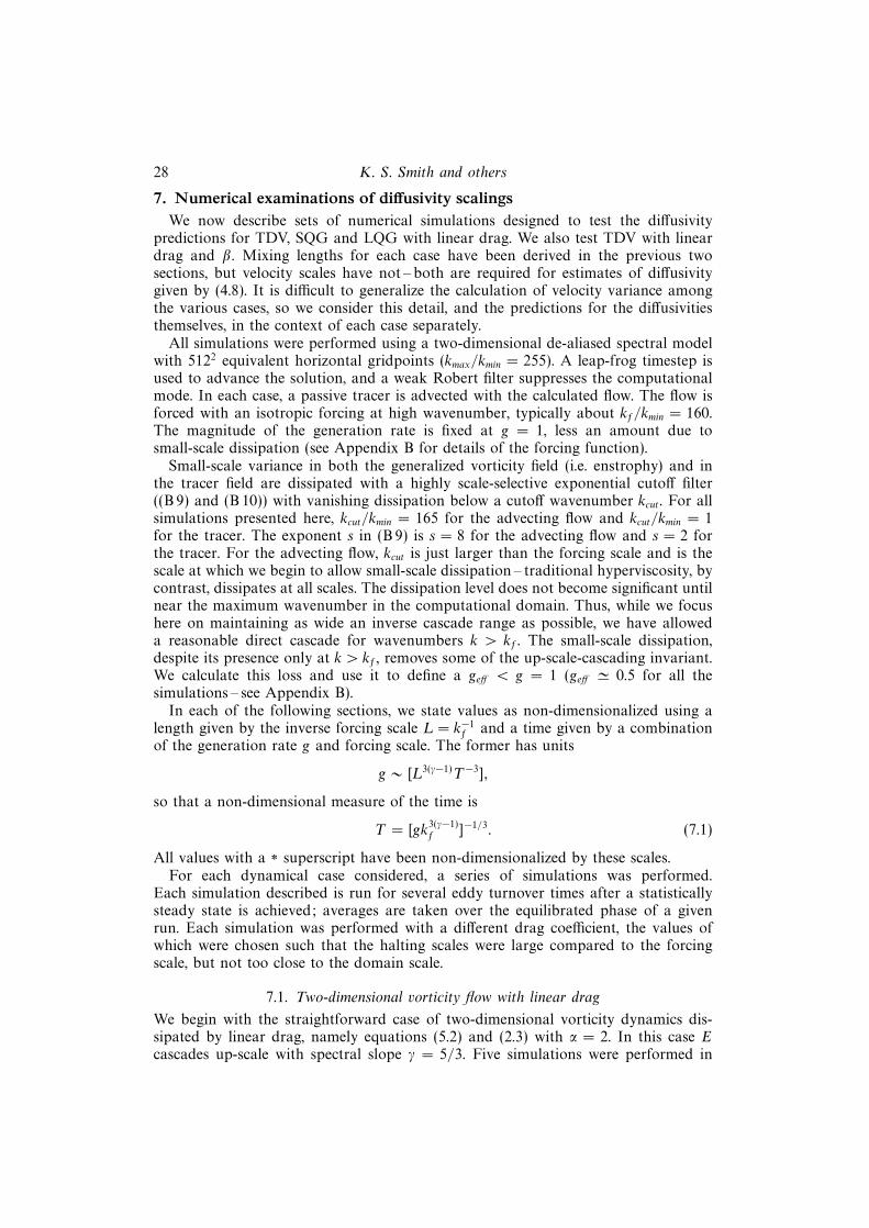
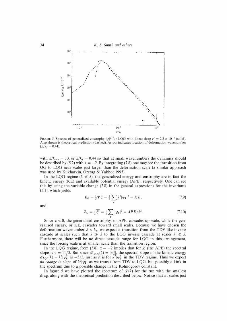
Figure 5. Spectra of generalized enstrophy |ψ|2 for LQG with linear drag r∗ = 2.3 × 10⁻⁴ (solid).Also shown is theoretical prediction (dashed). Arrow indicates location of deformation wavenumber(λ/kf = 0.44).
with λ/kmin = 70, or λ/kf = 0.44 so that at small wavenumbers the dynamics shouldbe described by (5.2) with α = −2. By integrating (7.8) one may see the transition fromQG to LQG near scales just larger than the deformation scale (a similar approachwas used by Kukharkin, Orszag & Yakhot 1995).
In the LQG regime (k � λ), the generalized energy and enstrophy are in fact thekinetic energy (KE) and available potential energy (APE), respectively. One can seethis by using the variable change (2.8) in the general expressions for the invariants(3.1), which yields
EG = 12Ψξ = 1
2
∑k
k2|ψk|2 = KE, (7.9)
and
ZG = 12ξ2 = 1
2
∑k
|ψk|2 = APE/λ2. (7.10)
Since α < 0, the generalized enstrophy, or APE, cascades up-scale, while the gen-eralized energy, or KE, cascades toward small scales. Because we have chosen thedeformation wavenumber λ < kf , we expect a transition from the TDV-like inversecascade at scales such that k � λ to the LQG inverse cascade at scales k � λ.Furthermore, there will be no direct cascade range for LQG in this arrangement,since the forcing scale is at smaller scale than the transition region.
In the LQG regime, from (3.8), α = −2 implies that for Z (the APE) the spectralslope is γ = 11/3. But since ZLQG(k) = |ψ2
k|, the spectral slope of the kinetic energyELQG(k) = k2|ψ2
k| is −5/3, just as it is for k2|ψ2k| in the TDV regime. Thus we expect
no change in slope of k2|ψ2k| as we transit from TDV to LQG, but possibly a kink in
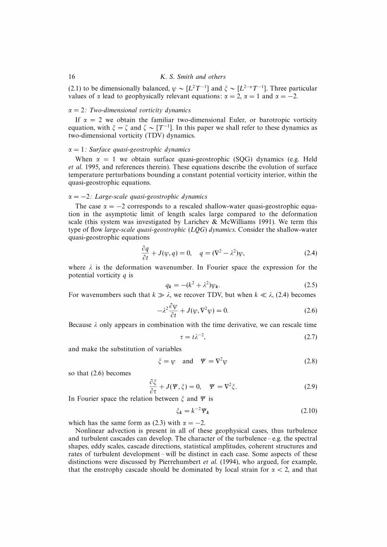
the spectrum due to a possible change in the Kolmogorov constant.In figure 5 we have plotted the spectrum of Z(k) for the run with the smallest
drag, along with the theoretical prediction described below. Notice that at scales just
Turbulent diffusion in the geostrophic inverse cascade 35
larger than the deformation scale (indicated by the arrow), the spectrum slumps butmaintains a similar slope, rising slightly near the spectral peak. Because of the limitedextent of the inertial range, an accurate determination of the appropriate Kolmogorovconstant is not possible, and we use the value from TDV, C = 6.
We expect the spectrum of generalized enstrophy to follow (5.20c) and the peak ofthis spectrum to be given by (5.23c). These expressions refer to the LQG formalismas derived in § 3, in which g is the generation rate of the generalized enstrophy.Dimensionally g ∼ [L8τ−3], where τ is the rescaled time coordinate (see equation(2.7)). Thus in terms of unscaled time, g̃ = λ6g, hence
kc = (C/4)3/8(r3λ6g̃−1)1/8, (7.11)
and
kr = (27C/44)3/8(r3λ6g̃−1)1/8, (7.12)
where g̃ is the familiar energy generation rate (the rate we set to unity in the numericalmodel). Since the spectral density has units Z ∼ [L9τ−2], we can also define a spectraldensity in unscaled time, Z̃ = λ4Z. But g̃2/3 = λ4g2/3 as well, so that the factors ofλ in the unscaled spectra only appear inside the expression for kc and kr . Finally,though, Z is a spectrum of |ψ|2/2, so the APE spectrum is expected to be
APE(k) = Cλ2g̃2/3k−11/3[1− (kc/k)8/3]2, (7.13)
with kc given by (7.11).From (7.9), the spectrum of kinetic energy is the spectrum of E(k) = k2Z(k), so the
total KE can be estimated
KE =
∫ ∞kr
k2Z(k) dk. (7.14)
The r.m.s. eddy meridional velocity V 2rms = KE (assuming isotropy) is thus predicted
to be
Vrms '(
33C3
4
g̃3
rλ2
)1/8
. (7.15)
Following (4.8) the diffusivity of the tracer is then
D '(
22
9
g̃
rλ2
)1/2
. (7.16)
Four simulations were performed, differing only in the value of the linear dragcoefficient. The non-dimensional values used were
r∗ = r(gk8f)−1/3 = rλ2(g̃k8
f)−1/3 = (0.035, 0.23, 1.4, 8.9)× 10−3.
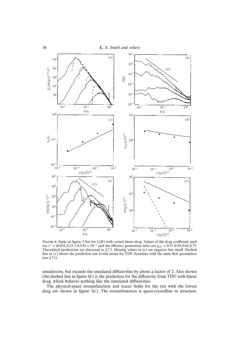
The spectra of APE, tracer variance and tracer flux, and the stopping scales, r.m.s.velocities and diffusivities, along with their respective theoretical predictions, areplotted in figure 6. At the largest scales, under which the assumptions used toderive LQG are most accurate, our theory predicts the spectral shape quite well. Thetracer spectra are more complicated, but still roughly follow their expected slopesof −5/3 (see discussion of LQG tracer in § 4). In the case with the smallest drag,the tracer flux spectrum is actually negative in the transition region k . λ, but weoffer no explanation for this behaviour. The stopping scales and r.m.s. velocitiesare also predicted somewhat successfully by our theory. Moreover, the divergenceof simulation from theory is very slight, even when the stopping scale is on orderthe deformation scale. The theoretical prediction for the diffusivity scales like the
36 K. S. Smith and others
103
102
101
100
10–2 10–1 100
k /kf
(a)
10–2 10–1 100
k /kf
(b)
–5/3
10–2
10–3
10–4
10–5
10–6
P(k
)
ZG
(k)/
(g k
f15/2
)2/3
(c) (d)
100
10–1
10–2
10–210–3
r /(g k f8)1/3
k0/k
f
V rm
s/g
kf5 )
1/3
101
100
10–210–4
r /(g k f8)1/3
(e) ( f )
10–210–4
r /(g k f8)1/3
10–2 10–1 100
k /kf
102
101
D/(
g k
f–2 )
1/3
102
101
100
D(k
)/(g
kf–1
)1/3
103
10–3
10–3
100
–5/3
104
10–1
10–510–410–5
10–1
10–2
10–5
Figure 6. Same as figure 2 but for LQG with varied linear drag. Values of the drag coefficient usedare r∗ = (0.035, 0.23, 1.4, 8.9)× 10−3 and the effective generation rates are geff = 0.57, 0.59, 0.62, 0.75.Theoretical predictions are discussed in § 7.3. Missing values in (e) are negative but small. Dashedline in ( f ) shows the prediction one would attain for TDV dynamics with the same flow parameters(see § 7.1).
simulations, but exceeds the simulated diffusivities by about a factor of 2. Also shown(the dashed line in figure 6f ) is the prediction for the diffusivity from TDV with lineardrag, which behaves nothing like the simulated diffusivities.
The physical-space streamfunction and tracer fields for the run with the lowestdrag are shown in figure 3(c). The streamfunction is quasi-crystalline in structure,
Turbulent diffusion in the geostrophic inverse cascade 37
and populated by deformation-scale vortices, as predicted by Kukharkin et al. (1995).This effect would presumably not be present had we simulated the strictly definedLQG equation rather than the shallow-water quasi-geostrophic equations. Despitethe predominance of small-scale ordered structures in the streamfunction, and theintermittency one would presume to accompany their presence, the spectrum is well-predicted by the inertial-range theory modified for linear drag. Moreover, and perhapsmore surprisingly, the tracer field is dominated by smooth plume-like structures whosecharacteristic scale is the energy-containing scale associated with the APE, ratherthan the deformation scale which strikes the eye in the physical-space image of thestreamfunction.
There is a wealth of phenomena in these simulations which require further researchto understand. The key point of the present investigation, however, has been todetermine the scale responsible for the mixing of a tracer.
7.4. Two-dimensional vorticity flow with linear drag and β
Lastly, we present the results of simulations of (6.1) with α = 2. We have no predictionfor the spectral shapes in this case, since we cannot derive a flux equation similarto (5.12) when β is present, but we do predict the jet scale, mixing length and r.m.s.velocity at the mixing scale (derived below). Note that now we have two independentparameters to consider: β and r.
In order to see the effects of β, drag must be set such that r . rc, where rc is definedby (6.7). In the simulations described here β is fixed such that the isotropic scale (6.5)lies within the computational domain at some relatively large wavenumber, but belowthe forcing wavenumber. The critical drag rc is then fixed by β and the generation rate(which is fixed for all simulations described in this paper). Five values of drag are thenchosen such that the largest value is just at rc while the rest are smaller. In this waywe hope to see a transition from the purely drag-induced diffusivity computed in § 7.1to the β-controlled diffusivity, which should be independent of drag. In particular, wechoose
β∗ ≡ β(gk5f)−1/3 = 0.73,
so that the inviscid β-scale (6.5) is (assuming a Kolmogorov constant C = 6 and aneffective generation of g = geff ' 0.5 – see Appendix A) kβ/kmin = 89, or
kβ/kf ' 0.56.
The non-dimensional critical drag, according to (6.7) (using the same values for gand C as above), is
r∗c ' 9.0× 10⁻².
The values of drag are then chosen to be
r∗ = (0.04, 0.43, 2.1, 4.3, 8.5)× 10−2
yielding predicted jet scales from (6.11) of
kβ,r/kf ' 0.18, 0.33, 0.48, 0.58, 0.69.
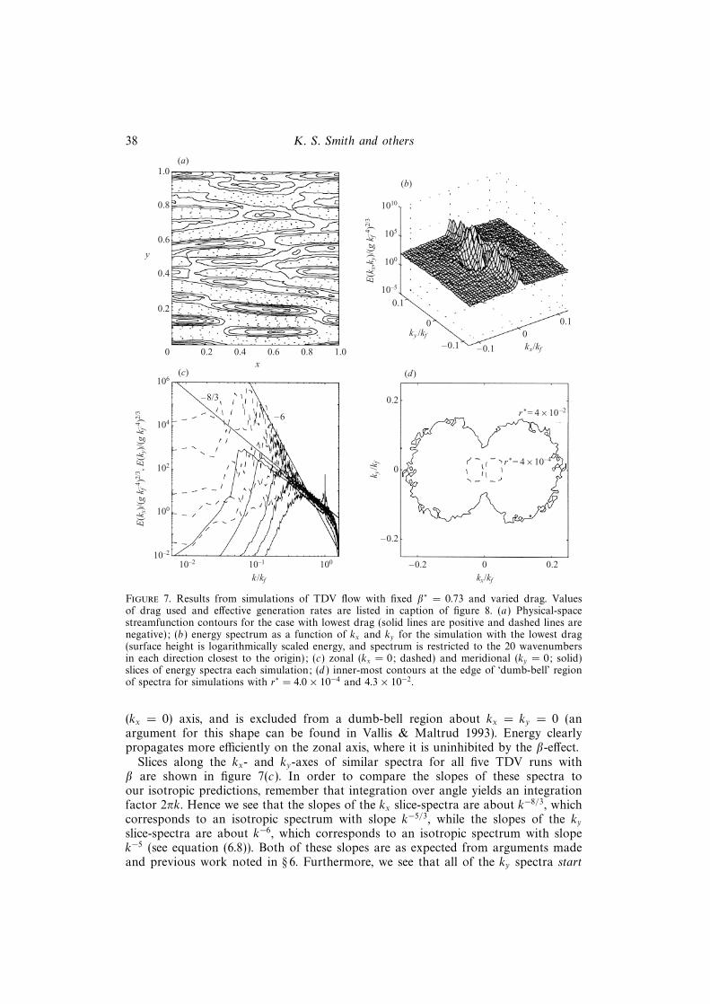
In figure 7 we try to give a sense of these flows before showing their statistics.Figure 7(a) shows a contoured snapshot of the physical-space streamfunction for thecase with the lowest drag, and demonstrates that the flow is dominated by zonal jets,as expected. The upper right panel contains the averaged two-dimensional energyspectrum for the same run. The surface height is the logarithm of the spectrum andonly the smallest wavenumbers are shown. Energy is concentrated along the zonal
38 K. S. Smith and others
1.0
0.8
0.6
0.4
0.2
0 0.2 0.4 0.6 0.8 1.0x
y
(a)
10–5
100
105
1010
0.1
0
–0.1 –0.1
00.1
kx/kf
ky /kf
(b)
E(k
x,k y
)/(g
kf–
4 )2/
3(c) (d)
E(k
x)/(
g k f–
4 )2/
3 , E
(ky)
/(g
k f–4 )
2/3
106
104
102
100
10–2
10–2 10–1 100
k /kf kx/kf
–0.2 0.20
–0.2
0
0.2
k y/k
f
–6
–8/3
r*= 4¬10–4
r*= 4¬10–2
Figure 7. Results from simulations of TDV flow with fixed β∗ = 0.73 and varied drag. Valuesof drag used and effective generation rates are listed in caption of figure 8. (a) Physical-spacestreamfunction contours for the case with lowest drag (solid lines are positive and dashed lines arenegative); (b) energy spectrum as a function of kx and ky for the simulation with the lowest drag(surface height is logarithmically scaled energy, and spectrum is restricted to the 20 wavenumbersin each direction closest to the origin); (c) zonal (kx = 0; dashed) and meridional (ky = 0; solid)slices of energy spectra each simulation; (d ) inner-most contours at the edge of ‘dumb-bell’ regionof spectra for simulations with r∗ = 4.0× 10⁻⁴ and 4.3× 10⁻².
(kx = 0) axis, and is excluded from a dumb-bell region about kx = ky = 0 (anargument for this shape can be found in Vallis & Maltrud 1993). Energy clearlypropagates more efficiently on the zonal axis, where it is uninhibited by the β-effect.
Slices along the kx- and ky-axes of similar spectra for all five TDV runs withβ are shown in figure 7(c). In order to compare the slopes of these spectra toour isotropic predictions, remember that integration over angle yields an integrationfactor 2πk. Hence we see that the slopes of the kx slice-spectra are about k−8/3, whichcorresponds to an isotropic spectrum with slope k−5/3, while the slopes of the kyslice-spectra are about k−6, which corresponds to an isotropic spectrum with slopek−5 (see equation (6.8)). Both of these slopes are as expected from arguments madeand previous work noted in § 6. Furthermore, we see that all of the ky spectra start
Turbulent diffusion in the geostrophic inverse cascade 39
to steepen at the same scale (the scale at which the −8/3 and −6 slopes cross),approximately k/kf = 0.56 ' kβ/kf , as predicted. (Since β is held constant, thisscale should be the same for all simulations.) Interestingly, energy cascades along thekx-axis past k ' kβ , typically peaking at about the same wavenumber, but with smallermagnitude, than the corresponding ky spectra. This phenomenon was also observedby, for example, Chekhlov et al. (1996) and Smith & Waleffe (1999), who point outthat despite the anisotropy present at large scale, an underlying isotropic cascade stilloccurs.
A sense of how the two-dimensional spectrum changes as drag is increased can begleaned from figure 7(d ), which shows the inner-most contours of energy values justshy of the maximum wavenumber along the kx-axis (so just inside the dumb-bell)for the case with the weakest drag (r∗ = 4 × 10⁻⁴) and the case with the second tolargest drag (r∗ = 4× 10⁻²). Despite the energy along the ky-axis starting to steepenat a fixed scale for all five simulations, the dumb-bell increases in size with increasingdrag coefficient.
Let us now consider the statistics of the flow. The peaks of the energy spectra alongthe ky-axis correspond to the jet scales, which we expected to be described by (6.11).If the isotropic β-scale kβ is the relevant mixing length, then despite the spectrumof meridional velocity extending past kβ , we require the meridional velocity at themixing scale in order to calculate the diffusivity. We estimate the turbulent meridionalvelocity near the mixing scale as
Vmix '[∫ ∞
kβ
E(k) dk
]1/2
'(
3
2
)1/2(C3g2
β
)1/5
. (7.17)
Then (6.5) and (7.17) imply a diffusivity
D '(
3
2
)1/2(C9/2g3
β4
)1/5
, (7.18)
which is independent of r.If, on the other hand, the jet scale kβ,r or (6.11) is the appropriate mixing length,
then we expect D ∼ r−1/4. Moreover, at values of drag r � rc, the diffusivity shouldroll over to the slope predicted for TDV dynamics with linear drag and no β, namelyD ∼ r−2.
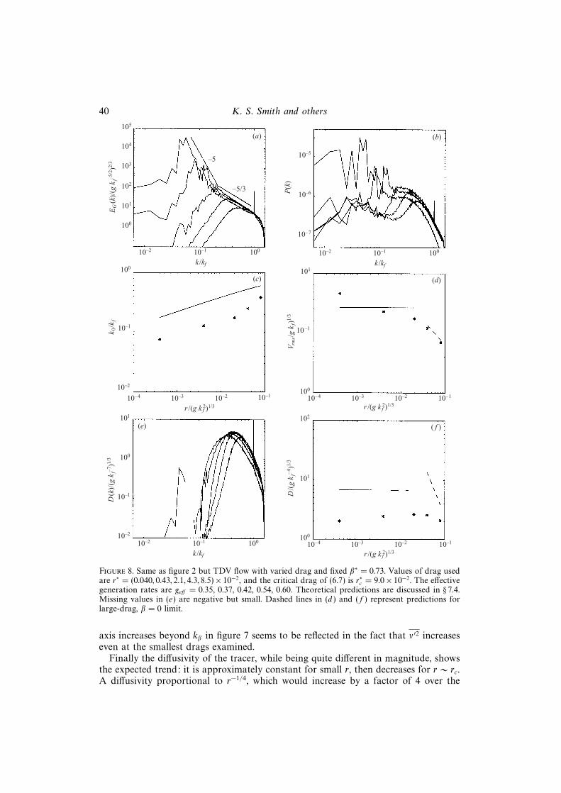
In figure 8 we plot the energy spectra, tracer variance and tracer flux as functionsof total wavenumber, and the jet scales (peaks along ky-axis), r.m.s. meridional eddyvelocities and integrated tracer fluxes, for the five simulations. The total energy spectrashow a break at a wavenumber slightly larger than kβ , where the spectra along theky-axis begin to steepen. The shape of these spectra can be best understood byreferring back to figure 7(c) – the contribution to the spectra in the region with slope−5 is almost solely due to zonal energy. Strikingly, there is no significant tracer fluxat scales larger than kβ – the spectra of the diffusivity (or tracer flux) vary only slightlyas drag is varied, but are essentially peaked at kβ . This supports our hypothesis thatkβ is the relevant meridional mixing length.
We also plot some predictions for the jet scales, r.m.s. velocities and diffusivities.The jet-scale is slightly over-predicted by kβ,r , but for the small-drag runs, the slope isclose to r1/4, as predicted by (6.11). At values of drag approaching rc, the slope of jetscale steepens. The meridional eddy velocity is somewhat flat at smaller values of r,but gently curves over the entire range. The fact that the spectrum along the ky = 0
40 K. S. Smith and others
103
102
101
100
10–2 10–1 100
k /kf
(a)
10–2 10–1 100
k /kf
(b)
–5/3
10–5
10–6
10–7
P(k
)
EG
(k)/
(g k
f–5/2
)2/3
(c) (d)
100
10–1
10–2
10–210–3
r /(g k f2)1/3
k 0/k
f
V rm
s/g
kf)
1/3
101
10–1
10–210–4
r /(g k f2)1/3
(e) ( f )
10–210–4
r /(g k f2)1/3
10–2 10–1 100
k /kf
102
101
D/(
g k
f–4 )
1/3
101
100
D(k
)/(g
kf–7
)1/3
10–3
10–3100
104
10–110–4 10–1
10–1
10–2
105
–5
10–1
100
Figure 8. Same as figure 2 but TDV flow with varied drag and fixed β∗ = 0.73. Values of drag usedare r∗ = (0.040, 0.43, 2.1, 4.3, 8.5)× 10−2, and the critical drag of (6.7) is r∗c = 9.0× 10⁻². The effectivegeneration rates are geff = 0.35, 0.37, 0.42, 0.54, 0.60. Theoretical predictions are discussed in § 7.4.Missing values in (e) are negative but small. Dashed lines in (d ) and ( f ) represent predictions forlarge-drag, β = 0 limit.
axis increases beyond kβ in figure 7 seems to be reflected in the fact that ν ′2 increaseseven at the smallest drags examined.
Finally the diffusivity of the tracer, while being quite different in magnitude, showsthe expected trend: it is approximately constant for small r, then decreases for r ∼ rc.A diffusivity proportional to r−1/4, which would increase by a factor of 4 over the
Turbulent diffusion in the geostrophic inverse cascade 41
range of r examined, is not seen, despite the fact that ν ′2 continues to increase slowlywith decreasing r. In fact, the diffusivity decreases slightly with decreasing r forthe smallest values examined. This implies that in the small-drag limit, the inviscid,isotropic β-scale kβ of (6.5), independent of drag, is a reasonable approximationto the mixing length for the diffusivity estimate. However, these estimates areclearly not as accurate in this anisotropic problem, where more sophisticated closures(e.g. resonant interaction theory) may help in obtaining quantitatively better fits.
8. ConclusionThis paper has been concerned with the inverse cascade in geostrophic turbulence,
and with the transport of a passive scalar by that turbulent fluid. We considered con-ventional two-dimensional (vorticity) dynamics, surface quasi-geostrophic dynamics,and large-scale quasi-geostrophic dynamics with a finite deformation radius.
We first showed that, for a general vorticity–streamfunction spectral field relation-ship of the form ξk = −kαψ, we may indeed expect forward and inverse cascades of ageneralized enstrophy and energy. In this context enstrophy refers to the variance ofthe advected field, and energy refers to the variance of the associated velocity. If α > 0(α < 0) then generalized energy will cascade to larger (smaller) scale and generalizedenstrophy to smaller (larger) scale. (The precise form of this statement is given inequations (A 9) and (A 10).) One notable aspect of this result is that, if α < 0 as forexample in large-scale geostrophic turbulence, the variance of the advected field istransferred to larger scales, in contrast to the usual passive-scalar-like behaviour of acascade to smaller scales.
Given the cascade directions, we can apply classical phenomenology to obtainpredictions of the spectral slope in each inertial range, the halting scale of theinverse cascade and, at a rather less-well-founded level, a prediction for a spectrum inthe inverse cascade that includes a frictional decay at small wavenumbers. The inversecascades will be modified and made anisotropic by the presence of a mean gradientof the advected quantity – the natural generalization of the familiar β-effect in TDV.However, because β cannot alter the overall energy level in barotropic flow, the inversecascade will only be halted by friction. (This situation should be contrasted with thebaroclinic case, in which eddy energies are a highly sensitive function of β because ofthe feedback between the energy injection rate and the mixing length – see, e.g. Held& Larichev 1996.) The anisotropy of the inverse cascade leads to two distinct lengthscales: a wavenumber (e.g. (6.11)) characterizing the scale of zonal flow, and a smallerscale (e.g. (6.5)) that characterizes the mixing length in the meridional direction.
From these predictions we construct estimates of the diffusion coefficient of apassive tracer field stirred by the turbulent fluid and whose variance is maintainedby a fixed meridional gradient. The expected dependences for the cases in which onlylinear drag is present are
TDV: D ∼ r−2,
SQG: D ∼ r−1 ln1/2(kf/kc), kc = (2C/3)(r3g−1)1/3,
LQG: D ∼ r−1/2,
and, in the small-drag limit when β is present,
TDV: D ∼ β−4/5,
SQG: D ∼ β−1 ln1/2(kf/kβ), kβ = βC−1/2g−1/3.
42 K. S. Smith and others
The last of these follows from using (6.4) for SQG as the mixing length, but was notderived nor tested here; the LQG case is special and we do not predict its diffusivebehaviour in the presence of β, notwithstanding its probable relevance to geophysicalflows. (See Kukharkin & Orszag 1996 for some treatment of this case.)
In each case in which linear drag halts the cascade, the diffusivity decreases withincreasing drag coefficient. This is perhaps not immediately obvious, since, fromthe perspective of Brownian motion for example, damping can act to increase theirreversibility of the flow for a given eddy energy. In turbulent inverse cascades,however, decreasing drag allows for increasing eddy scales, thus increasing the eddymixing length, and thereby increasing the diffusivity. On the other hand, when β issignificant relative to the drag (i.e. when r < rc in (6.6) or (6.7)), a diffusivity whichis increasing or constant with drag is reasonable. In this less-turbulent, more-wave-dominated parameter regime, zonal jets act as mixing barriers, and the underlyingflow is less irreversible. In this case, understanding and predicting the transport oftracer probably requires a different type of mathematical machinery than employedhere.
We have tested many of these predictions numerically. Overall, the predictionsfor the halting scale of the inverse cascade, and the velocity amplitude at the halt-ing scale, are quantitatively well-satisfied. We saw little evidence of non-universalbehaviour over a wide range of frictional parameters, providing that the inertialrange was well-developed and that the halting scale was substantially smaller thanthe domain scale, with no pile up of energy at the halting scale. If any of theseare not satisfied the predictions may fail. (Note also that all of our simulationsutilized a single type of forcing, namely a random stirring localized in wavenum-ber.) The form of the predicted spectrum is less well-satisfied by the numericalsimulations – the latter typically falling off much less rapidly than the former atsmall, frictionally dominated wavenumbers. However, because the flow in this low-wavenumber regime has little energy, it does not contribute to the meridional flux ofthe tracer.
Consistent with these results, the transport of a passive scalar advected by theturbulent flow is down-gradient diffusive, with a diffusion coefficient well-estimatedby turbulence phenomenology. In particular, for an isotropic inverse cascade, thediffusion coefficient is proportional to the product of the mixing length and the r.m.s.velocity amplitude, which are both determined by the halting scale of the inversecascade. In the presence of a β-effect, the inverse cascade can develop significantanisotropy; the mixing length appropriate to the meridional transport of a passivetracer scales more or less with the isotropic β-scale given by (6.5), whereas theenergy-containing scale is the jet scale (6.11).
Our predictions of the diffusion coefficients owe their approximate success to thepresence of a good scale separation between the mean gradient and the energy-containing scales, and a second scale separation between the energy-containing scaleand the forcing scale, enabling a well-defined inverse cascade to occur and minimizingthe effects of the forcing. Both of these conditions are formally necessary for simplescaling behaviour, but in many cases such scalings may well remain valid wellinto more weakly nonlinear regimes (e.g. Held & Larichev 1996). While neitherscale separation is particularly well-satisfied by meridional heat transport in theEarth’s atmosphere, scale separations between large-scale gradients and the internalradius of deformation are certainly significant in the Earth’s mid-oceans and on thegiant gas planets, and the present diffusivity predictions may be particularly useful inthose arenas.
Turbulent diffusion in the geostrophic inverse cascade 43
We acknowledge the contributions of A. Fournier to the tracer diffusivity calcula-tions, and thank B. Arbic, S. Danilov, D. Gurarie, P. Kushner and G. Lapeyre for veryhelpful comments. S. Danilov and D. Gurarie (preprint) have independently proposedand explored the scaling (6.11).
Appendix A. Phenomenology of cascade directionsWe first define a rescaled wavenumber k′ ≡ kα/2. In this space, the energy and
enstrophy spectra are such that
EG =
∫E′G(k′) dk′, (A 1a)
ZG =
∫Z′G(k′) dk′, (A 1b)
where
Z′G(k′) = k′2E′G(k′). (A 2)
The centroid of the energy distribution in this space is given by
k′e ≡
∫k′E′G(k′) dk′∫E′G(k′) dk′
. (A 3)
We now suppose that there is some initial distribution of energy distributed aroundthis wavenumber, and that turbulence acts irreversibly to broaden this distribution.That is,
I ′ =
∫(k′ − k′e)2E′G(k′) dk′, (A 4a)
dI ′
dt> 0. (A 4b)
Then, expanding (A 4a) and using (A 3),
I ′ =
∫(k′2 − k′2e )E′G(k′) dk′. (A 5)
Since dI ′/dt > 0, and both∫ E′G(k′) dk′ and
∫k′2E′G(k′) dk′ are constant, we must have
thatdk′2edt
< 0. (A 6)
This implies that
dkαedt
< 0, (A 7)
where kαe is a measure of the centre of the energy distribution in conventionalwavenumber space, given by
ke ≡
∫kα/2EG(k) dk∫EG(k) dk
2/α
. (A 8)
44 K. S. Smith and others
From (A 7) we immediately have
dkedt
< 0, α > 0
dkedt
> 0, α < 0.
(A 9)
It is because the mapping between the two wavenumber spaces is monotonic that amonotonic direction of energy or enstrophy transfer in the new wavenumber spacecorresponds to a monotonic transfer in the true wavenumber space, although therates of transfer (and the direction of transfer if α < 0) will differ.
Finally, we note that in the above derivations we may substitute ZG(k) for EG(k),and α → −α, in equations (A 8) onward. We then readily obtain the direction of thegeneralized enstrophy transfer,
dkzdt
> 0, α > 0
dkzdt
< 0, α < 0,
(A 10)
where, analogous to (A 8),
kz ≡
∫kα/2ZG(k) dk∫ZG(k) dk
2/α
. (A 11)
For TDV and SQG the generalized enstrophy, corresponding to the square of theadvected quantity, cascades to smaller scales and the energy cascades to larger scales.However, for LQG dynamics the generalized enstrophy (that is, the variance of theadvected quantity) cascades to larger scales, and generalized energy to smaller scales.This occurs in spite of the fact that the equation of motion is identical to that of apassive tracer, save for the additional constraint Ψ = ∇2ξ. This serves to emphasizethe point that inferring cascade directions in two-dimensional vorticity dynamics byanalogy to passive tracer dynamics is valid only to the extent that vorticity acts asa passive tracer. This may well be the case for small-scale vorticity, but it is not ageneral rule.
Appendix B. The numerical modelThe forcing function
The forcing is random Markovian in time and normalized at each timestep such thatg = 1. Specifically, at each wavenumber k and timestep n, we calculate an initialforcing function
F̂n = cFn−1 + (1− c2)1/2 eiθ, (B 1)
where θ is a random phase and c is the correlation coefficient, set to 0.99 in all cases.Since the generation rate is g = −ψF , in order to make g = 1 the actual forcing Fnis calculated as
Fn = −(ψF̂n
)−1
F̂n. (B 2)
Turbulent diffusion in the geostrophic inverse cascade 45
The effective forcing, however, is less than 1 due to some loss from the small-scalefilter, but this loss is restricted to scales smaller than the forcing scale. We calculatethis loss and find the effective generation rate via
geff = 1 + 〈ψDψ〉, (B 3)
where Dψ represents the filter dissipation and 〈 〉 means a time average. The latterterm quickly reaches a steady value (usually about 0.45) in all the simulations andthus the effective rate geff is well defined.
The enstrophy filter and timestep
The equation of motion is stepped forward via a leap-frog step but with the enstrophyfilter applied implicitly,
ξn+1 − ξn−1
2δt= Rn +H(k)ξn+1, (B 4)
where Rn represents the right-hand-side terms at time step n and δt is the magnitudeof the timestep. Thus
ξn+1 = (2δtRn + ξn−1)F(k), (B 5)
where
F(k) = [1 + 2δtH(k)]−1 (B 6)
is the filter.Although we do not use it, let us, as an example, consider a hyperviscosity filter of
order s, i.e. (−1)s/2+1νs∇sξ, then
H(k) = −νsks.Optimal estimates for the timestep and hyperviscosity are (see, e.g. Maltrud & Vallis1991)
δt ' 2π
Nk2−αmaxξrms
, νs ' (ξrms k2−αmax)k−smax. (B 7)
(This former estimate is used to calculate an adaptive timestep in the model.) Usingthese estimates in the hyperviscous filter then yields
Fhv(k) =
[1 +
4π
N
(k
kmax
)s]−1
, (B 8)
which is independent of the flow. N = 2kmax is the equivalent horizontal resolution.Note that F(0) = 1 and F(kmax) = (1 + 4π/N)−1, so that no dissipation happens onthe largest scale, and the maximum dissipation is a function only of the resolution.Furthermore, and sensibly, as N → ∞, F(kmax) → 1. Finally, the power s only affectsthe curvature of the filter – the higher the power, the less affected are the smallerwavenumbers (larger scales).
Loosely following LaCasce (1996, and personal communication) we construct anexponential cutoff filter with the explicit property of having absolutely no dissipationat wavenumbers smaller than some preset cutoff wavenumber, kcut. In particular,suppose we choose
Fec(k) =
{exp[−a(k − kcut)s], k > kcut
1, k 6 kcut.(B 9)
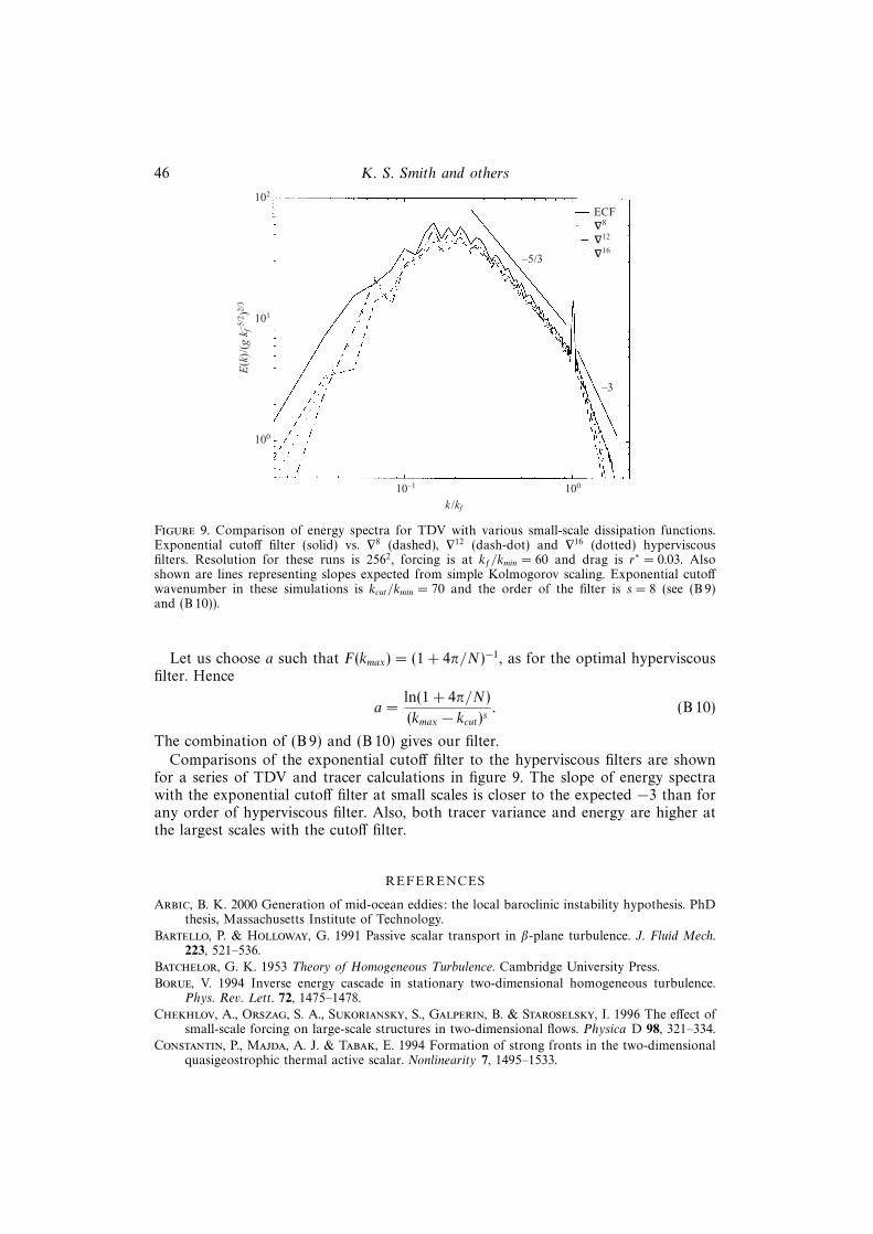
46 K. S. Smith and others
102
101
100
10–1 100
–3
–5/3
k /kf
E(k
)/(g
kf–5
/2)2/
3
ECF¡8
¡12
¡16
Figure 9. Comparison of energy spectra for TDV with various small-scale dissipation functions.Exponential cutoff filter (solid) vs. ∇8 (dashed), ∇12 (dash-dot) and ∇16 (dotted) hyperviscousfilters. Resolution for these runs is 2562, forcing is at kf/kmin = 60 and drag is r∗ = 0.03. Alsoshown are lines representing slopes expected from simple Kolmogorov scaling. Exponential cutoffwavenumber in these simulations is kcut/kmin = 70 and the order of the filter is s = 8 (see (B 9)and (B 10)).
Let us choose a such that F(kmax) = (1 + 4π/N)−1, as for the optimal hyperviscousfilter. Hence
a =ln(1 + 4π/N)
(kmax − kcut)s . (B 10)
The combination of (B 9) and (B 10) gives our filter.Comparisons of the exponential cutoff filter to the hyperviscous filters are shown
for a series of TDV and tracer calculations in figure 9. The slope of energy spectrawith the exponential cutoff filter at small scales is closer to the expected −3 than forany order of hyperviscous filter. Also, both tracer variance and energy are higher atthe largest scales with the cutoff filter.
REFERENCES
Arbic, B. K. 2000 Generation of mid-ocean eddies: the local baroclinic instability hypothesis. PhDthesis, Massachusetts Institute of Technology.
Bartello, P. & Holloway, G. 1991 Passive scalar transport in β-plane turbulence. J. Fluid Mech.223, 521–536.
Batchelor, G. K. 1953 Theory of Homogeneous Turbulence. Cambridge University Press.
Borue, V. 1994 Inverse energy cascade in stationary two-dimensional homogeneous turbulence.Phys. Rev. Lett. 72, 1475–1478.
Chekhlov, A., Orszag, S. A., Sukoriansky, S., Galperin, B. & Staroselsky, I. 1996 The effect ofsmall-scale forcing on large-scale structures in two-dimensional flows. Physica D 98, 321–334.
Constantin, P., Majda, A. J. & Tabak, E. 1994 Formation of strong fronts in the two-dimensionalquasigeostrophic thermal active scalar. Nonlinearity 7, 1495–1533.
Turbulent diffusion in the geostrophic inverse cascade 47
Danilov, S. & Gryanik, V. 2001 Vorticity structure, jets, and spectra in quasi-stationary beta-planeturbulence with a strong zonal component. Preprint.
Danilov, S. D. & Gurarie, D. 2000 Quasi-two-dimensional turbulence. Usp. Fiz. Nauk. 170, 921–968.
Danilov, S. & Gurarie, D. 2001 Nonuniversal features of forced two-dimensional turbulence inthe energy range. Phys. Rev. E 63, 020203:1–4.
Galperin, B., Sukoriansky, S. & Huang, H. P. 2001 Universal n−5 spectrum of zonal flows ongiant planets. Phys. Fluids 13, 1545–1548.
Held, I. M. & Larichev, V. D. 1996 A scaling theory for horizontally homogeneous, baroclinicallyunstable flow on a beta-plane. J. Atmos. Sci. 53, 946–952.
Held, I. M., Pierrehumbert, R. T., Garner, S. T. & Swanson, K. L. 1995 Surface quasi-geostrophicdynamics. J. Fluid Mech. 282, 1–20.
Huang, H. P., Galperin, B. & Sukoriansky, S. 2001 Anisotropic spectra in two-dimensionalturbulence on the surface of a rotationg sphere. Phys. Fluids 13, 225–240.
Kolmogorov, A. N. 1941 The local structure of turbulence in incompressible viscous fluid for verylarge Reynolds numbers. Dokl. Acad. Sci. USSR 30, 299–303.
Kraichnan, R. & Montgomery, D. 1980 Two-dimensional turbulence. Rep. Prog. Phys. 43,547–619.
Kukharkin, N. & Orszag, S. A. 1996 Generation and structure of Rossby vortices in rotatingfluids. Phys. Rev. E 54, 4524–4527.
Kukharkin, N., Orszag, S. A. & Yakhot, V. 1995 Quasicrystallization of vortices in drift-waveturbulence. Phys. Rev. Lett. 75, 2486–2489.
LaCasce, J. H. 1996 Baroclinic vortices over a sloping bottom. PhD thesis, Massachusetts Instituteof Technology.
Larichev, V. D. & Held, I. M. 1995 Eddy amplitudes and fluxes in a homogeneous model of fullydeveloped baroclinic instability. J. Phys. Oceanogr. 25, 2285–2297.
Larichev, V. D. & McWilliams, J. C. 1991 Weakly decaying turbulences in an equivalent-barotropicfluid. Phys. Fluids A 3, 938–950.
Leith, C. E. 1967 Diffusion approximations for two-dimensional turbulence. Phys. Fluids 11,671–674.
Lilly, D. K. 1972 Numerical simulation studies of two-dimensional turbulence. Geophys. Astrophys.Fluid Dyn. 3, 289–319.
Lindborg, E. & Alvelius, K. 2000 The kinetic energy spectrum of the two-dimensional enstrophyturbulence cascade. Phys. Fluids 12, 945–947.
Maltrud, M. E. & Vallis, G. K. 1991 Energy spectra and coherent structures in forcedtwo-dimensional and beta-plane turbulence. J. Fluid Mech. 228, 321–342.
Manfroi, A. J. & Young, W. R. 1999 Slow evolution of zonal jets on the beta plane. J. Atmos. Sci.56, 784–800.
Newell, A. C. 1969 Rossby wave packet interactions. J. Fluid Mech. 35, 255–271.
Oetzel, K. & Vallis, G. K. 1997 Strain, vortices, and the enstrophy inertial range in two-dimensionalturbulence. Phys. Fluids 9, 2991–3004.
Pedlosky, J. 1987 Geophysical Fluid Dynamics, 2nd edn. Springer.
Pierrehumbert, R. T., Held, I. M. & Swanson, K. L. 1994 Spectra of local and nonlocaltwo-dimensional turbulence. Chaos, Solitons Fractals 4, 1111–1116.
Rhines, P. B. 1975 Waves and turbulence on a β-plane. J. Fluid Mech. 69, 417–443.
Rhines, P. B. 1977 The dynamics of unsteady currents. In The Sea (ed. E. A. Goldberg, I. N.McCane, J. J. O’Briend & J. H. Steele), vol. 6, pp. 189–318. J. Wiley and Sons.
Rivera, M. & Wu, X. L. 2000 External dissipation in driven two-dimensional turbulence. Phys. Rev.Lett. 5, 976–979.
Salmon, R. 1980 Baroclinic instability and geostrophic turbulence. Geophys. Astrophys. Fluid Dyn.10, 25–52.
Schorghofer, N. 2000 Energy spectra of steady two-dimensional flows. Phys. Rev. E 61, 6572–6577.
Smith, L. M. & Waleffe, F. 1999 Transfer of energy to two-dimensional large scales in forced,rotating three-dimensional turbulence. Phys. Fluids 11, 1608–1622.
Smith, L. M. & Yakhot, V. 1993 Bose condensation and small-scale structure generation in arandom force driven two-dimensional turbulence. Phys. Rev. Lett. 71, 352–355.
48 K. S. Smith and others
Sukoriansky, S., Galperin, B. & Chekhlov, A. 1999 Large scale drag representation in simulationsof two-dimensional turbulence. Phys. Fluids 11, 3043–3053.
Tennekes, H. & Lumley, J. L. 1994 A First Course in Turbulence. MIT Press.
Vallis, G. K. 1993 Problems and phenomenology in two-dimensional turbulence. In NonlinearPhenomena in Atmospheric and Oceanic Sciences (ed. C. F. Carnevale & R. Pierrehumbert), pp.1–25. Springer.
Vallis, G. K. & Maltrud, M. E. 1993 Generation of mean flows and jets on a beta plane and overtopography. J. Phys. Oceanog. 23, 1346–1362.