time variations paper - southwest research...
TRANSCRIPT

Manuscript Revision: McComas et al. The evolving outer heliosphere: Large-scale stability and time variations observed by IBEX
The evolving outer heliosphere: Large-scale stability and time
variations observed by the Interstellar Boundary Explorer
1
2
3
4
5
6
7
8
9
10
11
12
13
14
15
16
17
18
19
20
21
22
23
D.J. McComas1,2, M. Bzowski3, P. Frisch4, G.B. Crew5, M.A. Dayeh1, R. DeMajistre6,
H.O. Funsten7, S.A. Fuselier8, M. Gruntman9, P. Janzen10, M.A. Kubiak3, G. Livadiotis1,
E. Möbius11, D.B. Reisenfeld10, N.A. Schwadron12,1
1 Southwest Research Institute, P.O. Drawer 28510, San Antonio, TX 78228, USA
2 University of Texas at San Antonio, San Antonio, TX 78249, USA
3 Space Research Centre of the Polish Academy of Sciences, Bartycka 18A, 00-716,
Warsaw, Poland
4 University of Chicago, Department of Astronomy and Astrophysics, 5640 S. Ellis Ave.,
Chicago, IL 60637, USA
5 Massachusetts Institute of Technology, Kavli Institute for Astrophysics and Space
Research, 77 Massachusetts Avenue, 37-515, Cambridge, MA, 02139, USA
6 Applied Physics Laboratory, Johns Hopkins University,11100 Johns Hopkins Road,
Laurel, MD 20723, USA
7 Los Alamos National Laboratory, Los Alamos, Bikini Atoll Rd., SM 30, NM 87545, USA
8 Lockheed Martin Advanced Technology Center, 3251 Hanover St, Palo Alto, CA 94304,
USA
9 University of Southern California, Division of Astronautical Engineering, Viterbi
School of Engineering, RRB 224, 1192, Los Angeles, CA 90089, USA
10 University of Montana, 32 Campus Drive, Missoula, MT, USA
- 1 -

Manuscript Revision: McComas et al. The evolving outer heliosphere: Large-scale stability and time variations observed by IBEX
11 University of New Hampshire, Space Science Center, Morse Hall Rm 407, Durham,
NH 03824, USA
24
25
26
27
28
29
30
31
32
33
34
35
36
37
38
39
40
41
42
43
44
45
46
12 Boston University, 725 Commonwealth Avenue, CAS Bulding, Room 515, Boston, Mass,
02215 USA
Abstract. The first all-sky maps of Energetic Neutral Atoms (ENAs) from the Interstellar
Boundary Explorer (IBEX) exhibited smoothly varying, globally distributed flux and a
narrow “ribbon” of enhanced ENA emissions. In this study we compare the second set of
sky maps to the first in order to assess the possibility of temporal changes over the six
months between views of each portion of the sky. While the large-scale structure is
generally stable between the two sets of maps, there are some remarkable changes that
show that the heliosphere is also evolving over this short timescale. In particular, we find
that 1) the overall ENA emissions coming from the outer heliosphere appear to be
slightly lower in the second set of maps compared to the first, 2) both the north and south
poles have significantly lower (~10-15%) ENA emissions in the second set of maps
compared to the first across the energy range from 0.5-6 keV, and 3) the “knot” in the
northern portion of the ribbon in the first maps is less bright and appears to have spread
and/or dissipated by the time the second set was acquired. Finally, the spatial distribution
of fluxes in the southern-most portion of the ribbon has evolved slightly, perhaps moving
as much as 6º (one map pixel) equatorward on average. The observed large-scale stability
and these systematic changes at smaller spatial scales provide important new information
about the outer heliosphere and its global interaction with the galaxy and help inform
possible mechanisms for producing the IBEX ribbon.
- 2 -

Manuscript Revision: McComas et al. The evolving outer heliosphere: Large-scale stability and time variations observed by IBEX
1. Introduction 47
48
49
50
51
52
53
54
55
56
57
58
59
60
61
62
63
64
65
66
67
68
69
The Interstellar Boundary Explorer (IBEX) mission (see McComas et al. [2009a] and
other papers in the IBEX Special Issue of Space Science Reviews) recently provided the
first global observations of the heliosphere’s interstellar interaction. These observations
included energy-resolved, all-sky images of energetic neutral atoms (ENAs) over the
energy range from ~0.1-6 keV, emanating from the outer heliosphere [McComas et al.,
2009b; Fuselier et al., 2009; Funsten et al., 2009a; Schwadron et al., 2009]. Generally
speaking, while some aspects of IBEX ENA observations were consistent with prior
expectations, many were not. In particular, IBEX discovered a narrow “ribbon” of
significantly enhanced ENA emissions passing between the directions of the two
Voyager spacecraft in the sky. Additional observations at higher energies from the
Cassini spacecraft [Krimigis et al., 2009] indicate a broader band of enhanced emissions
that generally lies close to the IBEX ribbon near the equator and in the northern
hemisphere, but deviates significantly from the ribbon in the south. Finally, the first
direct measurements of interstellar neutral H and O were also made by IBEX [Möbius et
al., 2009]. In this study, we provide new ENA observations from IBEX, covering its
complete second set of sky maps, and focus on determining if and how these maps (and
the outer heliosphere itself) may be evolving over short (half-year) timescales.
The narrow ribbon discovered by IBEX is superposed on a globally distributed ENA flux
that is organized by ecliptic latitude and longitude (essentially solar latitude and the
direction of motion with respect to the local interstellar medium, LISM) [McComas et al.,
2009b; Fuselier et al., 2009; Funsten et al., 2009a; Schwadron et al., 2009]. ENA fluxes
- 3 -

Manuscript Revision: McComas et al. The evolving outer heliosphere: Large-scale stability and time variations observed by IBEX
70
71
72
73
74
75
76
77
78
79
80
81
82
83
84
85
86
87
88
89
90
91
92
in the ribbon reach maxima ~2-3 times higher than the surrounding regions, and while the
ribbon is variable in width from <15º to >25º FWHM along its length [McComas et al.,
2009b; Fuselier et al., 2009], it averages ~20º wide over a broad energy range of IBEX’s
energy steps centered on energies from 0.7-2.7 keV [Fuselier et al., 2009]; this analysis
did not remove the intrinsic width of the IBEX sensors’ angular response (~7º FWHM),
so the real average width of the ribbon is actually thinner <20º. Even more remarkably,
the ribbon also shows statistically significant fine structure that is at most a few degrees
across [McComas et al., 2009b]. The center of the ribbon passes ~25º away from the
upwind direction or “nose” of the heliosphere and has brighter emissions from somewhat
broader regions at higher latitudes in both hemispheres - around ~60º N and ~40º S
ecliptic latitudes [McComas et al., 2009b; Funsten et al., 2009a]. The northern bright
region or “knot” has a different spectral shape than the rest of the ribbon with an
enhancement (bump) at higher energies, consistent with the shape of other near-pole
energy spectra [Funsten et al., 2009a]. In fact, the ribbon has nearly the same average
spectral slope and shape as surrounding regions at all heliolatitudes [McComas et al.,
2009b; Funsten et al., 2009a].
One of IBEX’s remarkable discoveries about the ribbon is that it appears to be ordered by
the most likely direction of the interstellar magnetic field just outside the heliopause (B),
and in particular seems to lie where B is nearly perpendicular to IBEX’s radially directed
(r) line of sight (LOS) – that is where B·r = 0 [McComas et al., 2009b; Schwadron et al.,
2009]. This direction is based on inferred flow deflections between interstellar H and He
[Lallement et al., 2005], which are also consistent with the direction inferred from 2-3
- 4 -

Manuscript Revision: McComas et al. The evolving outer heliosphere: Large-scale stability and time variations observed by IBEX
kHz radio emissions measured by the Voyager spacecraft [Gurnett et al., 2006]. The
model of the draped, local magnetic field [Pogorelov et al., 2009] that very closely
matches the IBEX ribbon [Schwadron et al., 2009] incorporates these flow deflections,
the observed ~10 AU difference between the termination shock (TS) crossing distances
of Voyagers 1 and 2 [Stone et al., 2008], and the inferred interstellar densities just outside
the heliosphere [Slavin and Frisch, 2008; Bzowski et al., 2008].
93
94
95
96
97
98
99
100
101
102
103
104
105
106
107
108
109
110
111
112
113
114
The ribbon weakens, but continues to extend around the north ecliptic pole, nearly
closing a loop on the sky [McComas et al., 2009b; Funsten et al., 2009a; Schwadron et
al., 2009]. The “center” of this loop in the first set of IBEX sky maps is at ~39° ecliptic
latitude and ~221° ecliptic longitude [Funsten et al., 2009a]. Ultimately, the combination
of simulations of detailed draping and compression of the interstellar field [e.g.,
Pogorelov et al., 2009; Schwadron et al., 2009 and references therein] with multiple sets
of all-sky maps from IBEX will likely provide the most accurate direction of the local
interstellar magnetic field.
The IBEX observations show the brightest regions of ribbon at mid to high latitudes,
where slow and fast solar winds interact in corotating interaction regions (CIRs). Thus, it
seems likely that the ribbon emissions are at least partially related to the solar wind
properties as well as to the external environment. Finally, as pointed out by McComas et
al. [2009b], while the ribbon appears as a generally continuous region of emissions, it
could easily be a string of localized and sometimes overlapping “knots” of emission. In
- 5 -

Manuscript Revision: McComas et al. The evolving outer heliosphere: Large-scale stability and time variations observed by IBEX
115
116
117
118
119
120
121
122
123
124
125
126
127
128
129
130
131
132
133
134
135
136
137
fact, the fine structure in the ribbon suggests that whatever mechanism creates the ribbon
emissions must be highly spatially variable.
Various possible explanations for the source of the ribbon were identified by McComas et
al. [2009], with additional analysis on several of these provided by Fuselier et al. [2009],
Funsten et al. [2009a], and Schwadron et al. [2009]. These explanations spanned
possibilities of how the ribbon emissions might be generated in the inner heliosheath
(between the TS and heliopause) in the solar wind (inside the TS), and in the outer
heliosheath (beyond the heliopause). The six possible sources of the IBEX ribbon
identified and briefly discussed by McComas et al. [2009b] are summarized
schematically in Figure 1 and described below:
(1) Maximum Pressure and Stagnation
The first general area of possible explanations centers on the observations of enhanced
particle pressure within the ribbon [McComas et al., 2009; Funsten et al., 2009a;
Schwadron et al., 2009]. This enhanced pressure could be generally balanced by
enhanced external pressure from the combination of the external plasma dynamic and
magnetic (JxB) forces, producing a localized band of maximum total pressure around the
heliopause. Such enhanced pressure at the heliopause might propagate throughout the
inner heliosheath, adjusting the plasma properties and bulk flow in such a way that the
ribbon might indicate the true region of highest pressure in the inner heliosheath. If so,
the flow would stagnate in this region and ion densities and ENA emissions would be
enhanced. As pointed out by McComas et al. [2009b], if the ribbon does represent the
- 6 -

Manuscript Revision: McComas et al. The evolving outer heliosphere: Large-scale stability and time variations observed by IBEX
138
139
140
141
142
143
144
145
146
147
148
149
150
151
152
153
154
155
156
157
158
159
160
region of highest pressure, then it would divide flows through the inner heliosheath,
analogous to a continental divide, which might explain the unusual flow directions
observed at the locations of the two Voyager spacecraft in the inner heliosheath.
An extension of this concept discussed by these authors was that the additional pressure
might also extrude small regions of the heliopause forming limited outward bulges in the
heliopause in the regions where the field was laying most tightly along its surface; such
“herniations” might collect ions, producing very high densities and almost no bulk flow,
potentially explaining the observed fine structure. This general explanation could
naturally account for the fact that the ribbon has a very similar spectral slope and shape of
the surrounding regions, as the enhanced ENA flux would arise naturally from the
accumulation of particles already in the inner heliosheath. Simulations and observations
appear to be at odds with one another concerning this mechanism. On the other hand,
magnetohydrodynamic (MHD) simulations of the heliospheric interaction, including
kappa distributions to emulate effects of enhanced tails of higher-energy pickup ions
[Prested et al., 2008; Izmodenov et al., 2009; Pogorelov et al., 2009], indicate maximum
pressure in the inner heliosheath near the nose and not along an extended region
significantly offset from the nose, such as the ribbon. Surely, the actual conditions in the
inner heliosheath are more complicated than accounted for in the current models, with (as
initially suggested by Zank et al. [1996]) a much smaller (~20% by number) pickup ion
population receiving the vast majority of the energization at the TS [Richardson et al.,
2008; 2009]. A start was made at more carefully addressing the role of the TS in
processing the solar wind and PUIs [Zank et al., 2010], however much more theoretical
- 7 -

Manuscript Revision: McComas et al. The evolving outer heliosphere: Large-scale stability and time variations observed by IBEX
161
162
163
164
165
166
167
168
169
170
171
172
173
174
175
176
177
178
179
180
181
182
183
work is needed in this area. Perhaps the complete treatment of this far more complicated
plasma in future simulations will reduce the discrepancies between the simulations and
observations.
(2) Primary ENAs from Compression
Another pair of related explanations [(2) and (3)] invoke the possibility of ribbon
emissions coming from outside the heliopause, from regions where the external B·r = 0
[McComas et al., 2009b; Schwadron et al., 2009] (see above). Compression of the
external field would increase densities and provide perpendicular heating, producing
more perpendicular pitch-angle distributions (enhanced particles around 90º pitch angles)
where they would preferentially emit in a plane that includes the inward radial direction.
Thus, local compressions in the outer heliosheath magnetic field would preferentially
emit ENAs that would be observable in the inner heliosphere by IBEX in exactly the
regions where the average external field is most perpendicular to the radial LOS.
(3) Secondary ENAs
In addition to interstellar ions, the external magnetic field is populated with particles from
ionization of outward traveling ENAs from both the solar wind region inside the TS and
the inner heliosheath. This source is labeled “secondary ENAs” as they have been
through the ion-to-ENA conversion process twice. These ions would have relatively
perpendicular pitch-angle distributions and be further compressed in regions where B·r =
0. The primary problem with this process for producing the ribbon, as pointed out by
McComas et al. [2009b], is that pitch-angle distributions would need to remain nearly
- 8 -
Manuscript Revision: McComas et al. The evolving outer heliosphere: Large-scale stability and time variations observed by IBEX
184
185
186
187
188
189
190
191
192
193
194
195
196
197
198
199
200
201
202
203
204
205
206
perpendicular for times comparable to or longer than neutralization times in the outer
heliosheath – times typically thought to be a few years. A simulation by Izmodenov et al.
[2009] including the secondary ENA source assumed comparatively rapid isotropization
and did not produce a ribbon-like structure. Since the publication of the IBEX results,
however, two different 3D MHD simulations [Heerikhuisen et al., 2010; Chalov et al.,
2010] have produced a structure very much like the overall ribbon structure by assuming
that perpendicular pitch-angle distributions can survive long enough for ions to re-
neutralize. If this assumption could somehow be validated, this secondary ENA process
would be a highly viable explanation for producing the ribbon. Finally, generating
observed fine structure in the ribbon with this process would further require bunched
ENAs produced by initially bunched solar wind ions or pickup ions, or additional small-
scale compressions of the magnetic field as discussed in (2).
(4) ENAs from Magnetic Reconnection at the Heliopause
Another possible mechanism identified by McComas et al. [2009b] was that ribbon
ENAs might result from magnetic reconnection across the heliopause. Reconnection
would allow hot heliosheath ions to propagate out into cooler, denser outer heliosheath
plasma. Magnetic reconnection could produce narrowly confined magnetic structures
potentially consistent with both “knots” and fine structure observed in the ribbon. The
external pressure is greatest along the ribbon [Schwadron et al., 2009], which generally
enhances the rate of magnetic reconnection. However, the magnetic field in the inner
heliosheath is highly variable [Burlaga et al., 2006], and average the field just inside of
the heliopause is expected to be “painted” with narrow alternating bands of oppositely
- 9 -

Manuscript Revision: McComas et al. The evolving outer heliosphere: Large-scale stability and time variations observed by IBEX
directed field [Suess, 2004], so it is not obvious why reconnection would be limited to a
narrow structure like the ribbon.
207
208
209
210
211
212
213
214
215
216
217
218
219
220
221
222
223
224
225
226
227
228
229
(5) ENAs from Shock-Accelerated Pickup Ions
Yet another possible mechanism discussed by McComas et al. [2009b] was that the
ribbon ENAs might be coming from the region around the TS, perhaps from shock-
accelerated pickup ions [Chalov and Fahr, 1996; Fahr et al., 2009] propagating inward
through the region where the solar wind decelerates significantly (~20%) in the last ~10
AU just inside the TS [Richardson et al., 2008]. Again, however, it is not obvious why
this mechanism would produce a ribbon instead of broadly distributed regions of
enhanced emissions.
6) ENAs from Heliopause Instabilities
Finally, McComas et al. [2009b] suggested that large-scale, Rayleigh-Taylor and/or
Kelvin–Helmholtz-like instabilities might confine hot, inner-heliosheath plasma in
narrow structures along the heliopause boundary. Such instabilities can be driven by
neutrals destabilizing the boundary. Some models [e.g., Borovikov et al., 2008] produce
large (>10 AU), semicoherent structures with higher ion densities that move tailward at
tens of km s-1 along the heliopause boundary.
The various possible mechanisms are not mutually exclusive; in fact some combination
or combinations may well ultimately explain the ribbon. One such example that is being
actively pursued [Kucharek et al., in preparation] combines (1) and (5). If a pressure
- 10 -
Manuscript Revision: McComas et al. The evolving outer heliosphere: Large-scale stability and time variations observed by IBEX
230
231
232
233
234
235
236
237
238
239
240
241
242
243
244
245
246
247
248
249
250
251
maximum (1) propagates through the inner heliosheath and indents the TS, ions that
specularly reflect off the indented part of the TS (as part of the shock-formation process)
will have gyro-velocity vectors directed back towards the Sun (5). ENAs produced by
charge exchange of these ions may account for the ribbon and fine structure within it.
While the basic mechanisms delineated above are under consideration for explaining the
IBEX ribbon, none produces the full range of observations without making significant,
unsubstantiated assumptions, and perhaps the ribbon arises from some completely
different mechanism. In fact, a seventh possible mechanism has been suggested by
Grzedzielski et al. [2010]. These authors propose a novel interpretation where the ribbon
does not arise from the heliospheric interaction at all, but instead from ENAs produced
by charge exchange between neutral H atoms at the nearby edge of the local interstellar
cloud (LIC) and hot protons from the Local Bubble. They argue that for reasonable
assumptions about local densities, such galactic ENAs should be able to reach the
heliosphere provided that the edge is close enough (less then ~500-2000 AU).
While IBEX data support some earlier ideas, in other areas a completely new paradigm is
needed for understanding the interaction between our heliosphere and the galactic
environment. This study examines the possibility of time evolution of the heliospheric
interaction in general and IBEX ribbon in particular, by comparing the first set of six-
month IBEX sky maps with the new set of maps generated over the subsequent six
months of observations. Observations of temporal evolution in IBEX ENA measurements
- 11 -

Manuscript Revision: McComas et al. The evolving outer heliosphere: Large-scale stability and time variations observed by IBEX
252
253
254
255
256
257
258
259
260
261
262
263
264
265
266
267
268 269
270
271
272
273
274
275
are pivotal for understanding this interaction in general and for testing the various
hypotheses that may account for the unexpected structures, such as the ribbon.
2. Observations from IBEX
IBEX is a spinning spacecraft with a spin rate of 4 RPM and spin axis (and solar array)
pointed toward the Sun. Each orbit (orbital period ~7.5 days) around perigee, the spin
axis is repointed back toward the Sun to compensate for the ~1º/day drift as the Earth
orbits the Sun. Therefore, observations from each orbit provide ~7º-wide “swaths”, at
multiple energies, that collectively produce a set of all-sky maps each six months. The
full width half maximum (FWHM) angular resolution of the IBEX ENA cameras is also
~7º, so, by design, the repointing and intrinsic angular resolution are roughly matched. In
this study we show observations from the IBEX-Hi sensor for energy steps (or
passbands) 2-6; Table 1 provides the nominal (peak) energy and energy range of each
energy step [Funsten et al., 2009b]. Detailed information about all aspects of the mission
is available in McComas et al. [2009a] and other papers in the IBEX Special Issue of
Space Science Reviews.
Figure 2 schematically shows the geometry of the IBEX orbit over the year. The Earth’s
magnetosphere (shaded) is oriented away from the Sun, so different seasons have quite
different magnetospheric backgrounds and obscuration. The first maps were made while
IBEX’s apogee was largely on the sunward side of Earth, where much of the time IBEX
was outside the Earth’s bow shock and in the solar wind. The second set of sky maps
were produced from orbits as IBEX’s apogee crossed through the magnetotail.
Commissioning of the IBEX-Hi sensor [Funsten et al., 2009b] was completed in Orbit 10,
- 12 -

Manuscript Revision: McComas et al. The evolving outer heliosphere: Large-scale stability and time variations observed by IBEX
276
277
278 279
280
281
282
283
284
285
286
287
288
289
290
291
292
293
294
295
296
297
298
299
so the first sky maps were taken over Orbits 11-33 (25 December 2008 through 18 June
2009), while the second were from Orbits 34-56 (18 June through 10 December 2009).
Figure 3 provides a comparison of the first (left) and second (right) sets of sky maps in
the spacecraft frame of reference. From top to bottom, the maps show data in the top five
energy channels of IBEX-Hi, labeled with the nominal central energies for each passband
(See Table 1). For each energy step, maps are compared using a consistent color scale.
While some corrections are required to make quantitative comparisons between maps at
each energy, the uncorrected observations in Figure 3 clearly show generally similar
ENA fluxes and the presence of the ribbon in roughly the same location for both the first
and second maps.
In order to quantitatively compare sky maps taken six months apart, we first consider
processes that could affect the measured fluxes of ENAs at IBEX. These include: 1) the
finite probability of ionization of ENAs on their way into 1 AU from the outer
heliosphere; 2) a very small energy change of ENAs due to the combined actions of solar
gravity and radiation pressure; and 3) the finite speed of the proper motion of the IBEX
detectors with respect to the Sun (the Compton-Getting effect). The first two of these
effects can be significant at lower energies, but only have very minor influence on the
ENAs in the energy ranges examined here (~0.5-6 keV). This is particularly true for quiet
times of the Sun and the solar wind, in which both the ionization probability and radiation
pressure are smallest. The past several years have been amongst the quietest times
observed with the most prolonged, lowest power interval of solar wind since the start of
the space age [McComas et al., 2008]. While these two effects are at work at all distances
- 13 -
Manuscript Revision: McComas et al. The evolving outer heliosphere: Large-scale stability and time variations observed by IBEX
300
301
302
303
304
305
306
307
308
309
310
311
312
313
314
315
316
317
318
319
320
321
322
along the trajectory of an ENA, they have the largest quantitative impact over the last ~10
AU as ENAs travel through the inner heliosphere approaching IBEX.
For this study, we calculated the combined effects of ionization and gravity/solar wind
pressure using recent solar observations from the Timed/SEE series (Lyman-alpha,
[Woods et al., 2005]), SOLAR 2000 (photoionization rate [Tobiska et al., 2000]), the
OMNI-2 time series (charge exchange with solar wind particles [King and Papitashvili,
2005]), and a model of the solar wind and radiation pressure latitude anisotropy [Bzowski,
2008]. We carried out the calculations for both spherically symmetric and latitude-
dependent solar wind structures following the approach proposed by Bzowski [2008],
who took into account (apart from the primary effects mentioned above) secondary
effects such as the Doppler dependence of the radiation pressure on the radial velocity of
the atoms due to the self-reversal of the solar Lyman-alpha line profile [Tarnopolski and
Bzowski, 2009], ionization by solar wind electrons [Bzowski et al., 2008], latitude
variation of the Lyman-alpha intensity [Auchere, 2005], and change of instantaneous
charge-exchange rate due to the change in relative velocity between the incoming ENA
and the expanding solar wind. The ecliptic 1 AU values of the relevant parameters are
shown in Figure 4. While there are a variety of short-duration fluctuations in these
parameters up to and including monthly (solar rotations) variations, the overall properties
are very similar over the intervals covering the first two sets of IBEX maps. One notable
exception is a solar wind event just before 2009.5, when a short, abrupt increase in solar
wind density (by a factor of ~6) occurred, resulting in a similar brief increase in the
charge-exchange rate.
- 14 -
Manuscript Revision: McComas et al. The evolving outer heliosphere: Large-scale stability and time variations observed by IBEX
323
324
325
326
327
328
329
330
331
332
333
334
335
336
337
338
339
340
341
342
343
344
Our model solar parameters as a function of heliolatitude are based on observations
obtained during the previous solar cycle [Bzowski et al., 2003; Bzowski, 2008]. Here we
calculate survival probabilities of H ENAs using this 3D model as well as validating the
3D results by comparing with a simpler 2D calculation where parameters do not depend
on heliolatitude. We examined the survival probabilities of H ENAs for the times and
geometry of IBEX observations used to construct the first two sets of IBEX maps for the
central energies of IBEX-Hi energy steps 2 through 6. Small latitude variations in
survival probability were obtained from the 3D calculation for ENAs approaching from
higher latitudes. Overall, however, the amplitude of latitudinal modulation due to
ionization (losses) of the ENAs in the supersonic solar wind are only a few percent and
thus have little impact on the IBEX maps.
We compared the survival probabilities for the time interval of the second set of IBEX
maps and calculated differences between the probabilities for the first and second sets of
maps. This comparison of survival probabilities shows that the effect on the survival
probabilities of violent and abrupt, but short-timed, events in the solar wind, such as the
event that happened shortly before 2009.5, is barely discernable. Figure 5 shows the
results of the 3D calculations where the ratio of survival probabilities is color coded as a
function of spacecraft spin phase and orbit number (from the second set of maps); ratios
for other energy steps are intermediate between the results shown here. The resulting
difference in survival probabilities between the equivalent orbits do not exceed 15% and
- 15 -
Manuscript Revision: McComas et al. The evolving outer heliosphere: Large-scale stability and time variations observed by IBEX
345
346
347
348
349
350
351
352
353
354
355
356
357
358
359
360
361
362
363
364
365
366
typically only ~5-10% for IBEX-Hi energy step 2 (the lowest one shown in this study).
For the rest of the higher-energy steps, these ratios are even smaller.
From our extensive calculations of these effects, we conclude that departures of
differences between the two sky maps of more than ~10% are most likely due to real
changes in the outer heliosphere and not modulation of ENAs propagating back through
the solar wind. In this study we chose to leave these corrections out of the IBEX data
being displayed in order to keep it as close as possible to the raw data and allow the
reader to independently assess the veracity of the temporal changes observed. One note of
caution for future studies of time variation is that the solar environment has been
unusually quiet since the start of IBEX observations. As the Sun becomes more active
and the solar wind more variable, these effects will become more significant and will
require the IBEX team to make explicit compensation or correction.
In contrast to the effects discussed above, we did need to make an explicit Compton-
Getting (CG) correction in order to quantitatively compare the first and second sets of
maps. This correction removes effects of the Earth’s (and IBEX spacecraft’s) ~30 km s-1
motion around the Sun. The CG correction is important because IBEX maps are taken in
a way that the same swath of the sky is observed exactly six months apart, when IBEX
has the opposite orbital velocity around the Sun and therefore needs the opposite CG
correction. The methodology for making the CG correction was developed and validated
through a consensus process within the IBEX team; the resulting CG correction
- 16 -
Manuscript Revision: McComas et al. The evolving outer heliosphere: Large-scale stability and time variations observed by IBEX
367
368
369
370
371
372
373
374
375
376
377
378
379
380
381
382
383
384
385
386
387
388
389
methodology is described briefly in Appendix A with a more complete development and
discussion in DeMajistre et al. [2010].
Figure 6 compares the first (left column) and second (middle column) sets of CG-
corrected ENA flux maps. Because the maps are corrected to common energies, it is now
possible to combine them for improved statistics for studies that are not attempting to
examine time evolution. The right column shows these combined, exposure-time-
weighted, averaged maps of ENA flux over an entire year; these maps have reduced
statistical errors in some parts of the sky where the sampling times in one or both of the
individual maps were extremely limited. An interesting feature revealed in the combined
maps is the clear extension of the ribbon toward a complete ring compared to what can be
seen in the individual sets of sky maps. These combined maps are available to the broad
community, and owing to the better coverage and statistics, we recommend them over the
individual first and second sets of sky maps for testing hypotheses derived through theory
and modeling that are not directly addressing time variations in the ENA flux.
With CG-corrected maps and common color bars shown in Figure 6, it is clear that the
gross ENA emissions observed at the ribbon and underlying globally distributed flux are
extremely stable over the six-month interval between the first and second sets of sky
maps. In order to better identify and visualize small differences between the two sets of
maps, Figure 7 shows equirectangular projected maps of the first (left) and second
(middle) sets of IBEX sky maps, highlighting specific intensity levels with red and white
outlines as indicated by the red and white arrows on each color bar, respectively. These
- 17 -

Manuscript Revision: McComas et al. The evolving outer heliosphere: Large-scale stability and time variations observed by IBEX
390
391
392
393
394
395
396
397
398
399
400
401
402
403
404
405
406
407
408
409
410
411
412
contours help guide the eye in comparing specific quantitative flux levels. Again, the
overall ribbon and general structure appear to be highly similar, although now, some
smaller differences are also apparent.
The third column of Figure 7 shows difference maps at each energy, where we have
subtracted the flux in each pixel of the first sky maps from the flux in the equivalent pixel
of the second sky maps. Red indicates higher ENA fluxes in the second map compared to
the first, or increasing flux over the six months between observations; similarly, blue
indicates decreasing flux over these six months. Several artificial features are evident in
the regular sky maps and amplified in these difference maps. In particular, the rectangular
maps enable identification of vertical stripes that correspond to an apparent enhanced
ENA flux throughout the swath acquired over a single orbit. These result from an
abnormally high and mostly uniform background present during most of an orbit or an
orbit with poor statistics due to removal of time intervals of high background during an
orbit. These features are particularly evident over longitude ranges of ~70º to 90º and
~180º to -150º.
Additionally, there is still a discontinuity in fluxes at angles of ~0º and ~180º, where the
first (11 and 34) and last (33 and 56) orbits of each map abut each other. This was far
more significant in the uncorrected images (Figure 3) compared to the CG corrected ones
(Figure 6) showing that this correction has largely accounted for the differences in flux.
However, in the difference maps of Figure 7, one can still see a general redness in the
hemisphere between ~0º and ~180º and general blueness in the opposite hemisphere,
- 18 -
Manuscript Revision: McComas et al. The evolving outer heliosphere: Large-scale stability and time variations observed by IBEX
413
414
415
416
417
418
419
420
421
422
423
424
425
426
427
428
429
430
431
432
433
434
435
especially at lower latitudes and in the lower energies. This could represent a real change
in the globally distributed ENA flux being observed by IBEX, with increasing ENA
emissions from the nose and decreasing emissions from the tail between the two sets of
maps. However, because the discontinuity occurs at angles of ~0º and ~180º, this
apparent difference is far more likely to be produced by imperfect CG correction of the
maps. A small systematic error in the CG correction (e.g., if there is still some residual
background noise in the lower-energy channels) will produce slight apparent asymmetries
between the ram and anti-ram viewing directions, especially at lower energies and
latitudes.
Notwithstanding the orbits with very low counting statistics and potentially imperfect CG
corrections, Figure 7 clearly shows some real differences between IBEX’s first and
second sets of sky maps. First, both the north and south polar regions have reduced ENA
fluxes in the second map compared to the first, as evidenced by the blue across the top
and bottom of the difference maps. The effect appears to be a significant reduction in
ENA flux over the six months between the two maps. Because the magnitude of the CG
correction is smaller at the higher energies and decreases with increasing latitude
(becoming zero at the poles), it can not be responsible for this observed change.
Figure 8 shows a more quantitative analysis of the change in high-latitude flux between
the first and second sets of sky maps. Here, we calculated exposure-weighted fluxes and
associated uncertainties in 2º latitudinal bands by summing over all azimuths. We then
integrated these fluxes and their uncertainties starting at both poles and including
- 19 -

Manuscript Revision: McComas et al. The evolving outer heliosphere: Large-scale stability and time variations observed by IBEX
436
437
438
439
440
441
442
443
444
445
446
447
448
449
450
451
452
453
454
455
456
457
458
increasing numbers of lower latitudinal bands. Thus, for each latitude in Figure 8, the
flux and associated uncertainty represent integrations of ENA observations poleward of
that latitude and over all longitudes.
The results in Figure 8 are extremely consistent, with both poles showing significantly
lower fluxes (left column) in the second maps at the various energies separately and for
all energies combined (bottom panels). The right column provides accumulated
uncertainties as the integrations extend to lower latitudes. Uncertainties decrease with
integration over an increasing range of latitudes down from the poles and reach minima
(~25º S and ~15º N from the poles – indicated by yellow regions) prior to growing as the
integrations start to include additional lower-latitude structure, such as the ribbon. By
using values around the uncertainty minima, this technique provides robust measures of
the differences in ENA flux from the two polar regions. Furthermore, the survival
probabilities are essentially identical for the polar regions, when integrated over all orbits
in the maps (see Figure 5). The overall reduction in flux at both poles is clear and
represents a decrease of ~10-15% over six months across the entire energy range from
~0.5-6 keV.
A second small change that can be seen in the sets of sky maps in Figure 7 are some
detailed spatial variations and an apparent northward motion of the southern, nearly
horizontal (roughly fixed latitude) portion of the ribbon, between longitudes of ~90º –
180º. This shows up both in differences between the locations of the contours in the left
and center columns and in the difference maps as a characteristic combination of a
- 20 -

Manuscript Revision: McComas et al. The evolving outer heliosphere: Large-scale stability and time variations observed by IBEX
459
460
461
462
463
464
465
466
467
468
469
470
471
472
473
474
475
476
477
478
479
480
481
decreased (blue) region immediately southward of an increased (red) region; these two
indicators show up to a greater or lesser extent in all five energy channels shown. This
apparent motion is only one pixel (~6º), which is the angular resolution of the IBEX
sensors. Thus, while consistent differences over a large longitude range and multiple
energies are highly suggestive of a real, albeit small, temporal change in the overall ENA
emissions, this change can not be considered definitive.
The third difference between the first two sets of IBEX sky maps, on the other hand, is a
clear change in the “knot” region in the northern portion of the IBEX ribbon [McComas
et al., 2009b; Funsten et al., 2009a], which exhibits flux enhancements at higher energies
in the first sky maps. In the second set of maps, this knot is substantially diminished and
appears to spread out both to lower latitudes at the same longitude and to higher latitudes
at longitudes away from the nose. Figure 9 magnifies the region of the 2.7 keV maps
around the knot. Contours at the same flux levels help guide the eye for changes between
the maps and again in the difference image (bottom panel), blue indicates a reduction and
red an enhancement over the six months between the maps. Clearly the ENA emissions
from the small region of the knot are substantially reduced in the second maps.
Additionally, there is some evidence for enhanced emissions in the second maps both
poleward along the ribbon (upper left red region in the difference image) and southward
(lower right red region in the difference image), compared to the first. The overall
reduction in the knot emissions are substantial, with roughly one fourth to one third less
emission observed over six months.
- 21 -

Manuscript Revision: McComas et al. The evolving outer heliosphere: Large-scale stability and time variations observed by IBEX
As one final quantitative comparison between the two sets of sky maps, we divided the
maps into three contiguous regions as shown in Figure 10: 1) the ribbon region,
encapsulated in a shell of width +/-18
482
483
484
485
486
487
488
489
490
491
492
493
494
495
496
497
498
499
500
501
502
503
504
o centered at ecliptic coordinates of 221o, 39o as
found by Funsten et al. [2009a]; 2) The nose and N pole region outside of the ribbon; and
3) the tail, flanks, and south pole region outside of the ribbon. Table 2 provides the ratio
of exposure-weighted averaged fluxes in the second set of CG-corrected all-sky maps
compared to the first set (6o x 6o pixels) for each pair of full maps and for these three
regions separately. The fluxes are time-exposure-weighted values based on all pixels
within each region; errors are calculated from error propagation of the standard
deviations of the fluxes. The overall ENA fluxes are reduced in the second set of maps
compared to the first. The errors shown, however, do not include non-statistical errors,
such as residual, unsubtracted backgrounds. While small, these backgrounds can have a
substantial impact on the lower-energy channels (gray), the effects of which are further
amplified by the CG-correction process, which is highly sensitive to the energy spectrum.
On the other hand, the results in the top two energies (>2 keV) are less effected and
indicate small reductions in the ENAs measured by IBEX.
3. Discussion
New observations from IBEX provided in this study show that:
1) The globally distributed ENA fluxes from the outer heliosphere are extremely stable
over the six months between observations in the first two sets of IBEX sky maps;
2) The ribbon of enhanced ENA flux is also extremely stable over the interval between
the first two maps.
- 22 -

Manuscript Revision: McComas et al. The evolving outer heliosphere: Large-scale stability and time variations observed by IBEX
505
506
507
508
509
510
511
512
513
514
515
516
517
518
519
520
521
522
523
524
525
526
527
However, some statistically significant differences indicate that the outer heliosphere is
noticeably evolving over this short (six month) timeframe. In particular:
3) The overall ENA emissions observed by IBEX above ~2 keV appear to be slightly
lower in the second set of sky maps compared to the first both within the ribbon and
outside of it;
4) Both the north and south poles have significantly lower (~10-15%) ENA emissions in
the second set of sky maps compared to the first across the energy range from 0.5-6 keV;
5) The “knot” in the northern portion of the ribbon in the first maps is less intense and
appears to have spread and/or somewhat dissipated by the time the second set of maps
was acquired;
6) The detailed fluxes in the southern (horizontal) portion of the ribbon have evolved and
there may be a slight (one pixel, ~6º) equatorward motion of its center.
The fact that both the globally distributed ENA flux and ENA emissions of the bright
ribbon are largely stable between IBEX’s first two sets of sky maps indicates a largely
stable heliospheric interaction and global configuration. It takes roughly one year for 1
keV solar wind to reach the TS at ~90 AU and then from half a year to nearly two years
for ENAs in the IBEX-Hi energy passbands to transit back ~100 AU from the inner
heliosheath (see Table 3); ENAs coming from the outer heliosheath, two to three times
further away take proportionally longer. Given the immense scale of the heliosphere and
its interstellar interaction, the many year time scales involved in plasma propagating
through this structure, and the anticipated long LOS integration paths producing ENAs in
the outer heliosphere, it would in fact have been far more surprising if the overall
structure was not largely stable for the short time of observations reported here. In future
- 23 -
Manuscript Revision: McComas et al. The evolving outer heliosphere: Large-scale stability and time variations observed by IBEX
528
529
530
531
532
533
534 535
536
537
538
539
540
541
542
543
544
545
546
547
548
549
550
studies, we plan to use time-lagged observations from various energies to reconstruct the
source fluxes in the outer heliosphere at fixed times in the past. Still, even with just the
first year of IBEX data, there are clear differences between the first two sets of maps,
indicating evolution of both globally distributed, and more localized, ribbon fluxes of
ENAs over only six months. Such variations likely indicate relatively thin source regions,
at least for the portions of the ENA emissions that are varying over this short timescale.
For the globally distributed flux, emissions from both polar regions were reduced by ~10-
15% over the six months between the first two maps. This reduction might be related to
decreasing solar wind flux over past several years [McComas et al., 2008] that should
decrease the density of the inner heliosheath. If these changes are caused by the evolution
of the global solar wind through the solar cycle then there may be as much as a factor of
two variation in ENA fluxes from the global heliosphere over the ~11-year solar cycle.
We note that the observation of polar evolution is a robust result because the CG
correction to the data is extremely small at the higher latitudes.
While it is possible that a second, apparent enhancement in the hemisphere toward the
nose (and reduction in the opposite hemisphere) could indicate real changes in the
globally distributed flux, such as an enhancement (decrease) in heliosheath thickness
and/or ion fluxes in nose (tail), we think it is far more likely that this apparent difference
is actually caused by an imperfect CG correction, which would have the largest effect at
the lowest energies and latitudes, as seen in the CG-corrected images.
- 24 -

Manuscript Revision: McComas et al. The evolving outer heliosphere: Large-scale stability and time variations observed by IBEX
In the ribbon, there are small but real variations between the maps, and thus time
evolution. The southern, horizontal portion of the ribbon appears to move northward
(toward the equator) possibly one pixel (6º), which is essentially the resolution of IBEX-
Hi. If this is actually a transverse motion of the source for this portion of the ribbon, then
for a source at ~100 AU, one pixel (6º) indicates a transverse speed of ~100 km s
551
552
553
554
555
556
557
558
559
560
561
562
563
564
565
566
567
568
569
570
571
572
573
-1; for a
source at ~250 AU, as suggested by the secondary ENA emission model (3), in the outer
heliosheath this would indicate a transverse speed of ~250 km s-1. Finally, this apparent
equatorward motion is opposite to what would be expected for convection of structures
away from the nose either along the heliopause or in the inner or outer heliosheath.
As discussed above, the ribbon occupies a region where the interstellar magnetic field in
the outer heliosheath is roughly perpendicular to the LOS [McComas et al., 2009b]; this
is the region for which B●r ~ 0, where B is the interstellar magnetic field that is
compressed in the outer heliosheath as the interstellar flow deflects around the heliopause
[Schwadron et al., 2009]. In fact, the compression of the interstellar flow shifts the
location of the ribbon from a great circle (with angular radius of 90°) into an arc with an
angular radius of <90° [Funsten et al., 2009a]. We expect that greater compression and
deflection of interstellar flow near the nose causes the region of B●r ~ 0 to decrease in
angular radius, therefore causing much of the ribbon to move equatorward, as observed.
This opens an important question about the potential for global changes in the properties
of the solar wind in the inner heliosheath to affect the deflection of interstellar flow
around the heliosphere, and therefore the location of the ribbon. For example, blunting of
the TS and heliopause, which may be related to a temporary (several year) reduction in
- 25 -

Manuscript Revision: McComas et al. The evolving outer heliosphere: Large-scale stability and time variations observed by IBEX
574
575
576
577
578
579
580
581
582
583
584
585
586
587
588
589
590
591
592
593
594
595
596
solar wind ram pressure, would lead to greater compression and deflection of interstellar
flow around the heliopause and, possibly, equatorward motion of the region where B●r ~
0.
The portion of the ribbon that shows clear time variation between the first two maps is
the knot in its northern region. Clearly, the brightest emissions at high energies in the first
set of sky maps are significantly diminished and spread out toward both higher and lower
latitudes; while the apparent spread northward and away from nose could be consistent
with convection away from nose, the southward enhancement is not. Evolution of the
knot indicates a spectral change, in which the flux in the central area of the knot has
become more like the adjacent sections of the ribbon and less like the most polar regions,
which all showed enhancements at the higher IBEX energies [Funsten et al., 2009a]. It is
interesting to consider if this change could be associated with the boundary between the
fast and slow solar wind regions moving and slower solar wind populating the inner
heliosheath at the latitude of the knot.
Given the largely stable structure, but clear evidence for evolution of at least some
portions of the ribbon, it is important to ask what the implications are for various
competing ideas about the source of the ribbon. Here we comment on each of the six
mechanisms suggested by McComas et al. [2009b] and discussed above, using the same
numbering system as in Figure 1:
(1) Maximum Pressure/Stagnation
- 26 -

Manuscript Revision: McComas et al. The evolving outer heliosphere: Large-scale stability and time variations observed by IBEX
597
598
599
600
601
602
603
604
605
606
607
608
609
610
611
612
613
614
615
616
617
618
619
In this explanation, the primary ribbon location should be generally stable owing to the
large-scale external pressure driver; however, changing internal pressure, for example
from small changes in the solar wind over time, could produce small changes in observed
ENA fluxes. Also, fine structure could be variable if produced by extrusions, which are
instabilities on the heliopause. Overall, based largely on the ribbon’s general stability,
this explanation appears consistent with the observations.
(2) Primary ENAs from Compressions
This concept is similar to (1) in that the large-scale structure would be expected to be
largely stable since it comes from the external pressure, but fine structure should vary
since it is mostly driven by small-scale compressional instabilities in the draped ISM
field, most likely close to the heliopause. In this case, the ribbon would likely be less
sensitive to solar wind changes than (1), since the ENA production occurs in the outer
heliosheath instead of the inner heliosheath. However, the fact that the population is
highly suprathermal indicates that it may be produced, at least partially, by secondary
ENAs (3), in which case the population would be sensitive to changes in the solar wind.
(3) Secondary ENAs
The mechanism is related to (2), but solar wind and inner heliosheath ENAs produce ions
that become re-neutralized, so solar wind changes are probably more visible. Also, this
process should occur continuously over large distances along the LOS (ionization
lengths: ~550 AU beyond the heliopause at 1 keV and ~900 AU at 5 keV owing to scale
lengths of ionization via charge exchange assuming a 0.07 cm-3 LISM proton density).
- 27 -

Manuscript Revision: McComas et al. The evolving outer heliosphere: Large-scale stability and time variations observed by IBEX
620
621
622
623
624
625
626
627
628
629
630
631
632
633
634
635
636
637
638
639
640
641
642
With the need to accumulate emission over a length >550 to 900 AU, this model has
trouble producing significant variations over times as short as six months. For example,
at 1 keV a secondary ENA takes ~6 years to transit the 550 AU ionization length, and
therefore >12 years to move from the solar wind into the LISM, and then back into the
heliosphere where it can be detected. Finally, this mechanism doesn’t produce fine
structure unless combined with (2), in which case it could be variable.
If the ribbon is formed outside the heliopause, then its location will shift with temporal
variations in ENA energies. The locus of sightlines that are perpendicular to the
interstellar magnetic field lines, B●r=0, varies with distance beyond the heliopause as
field lines bend around the heliosphere. The energy-dependent mean free paths of ENAs
therefore should affect the location of the ribbon’s arc. The finite widths of the IBEX-Hi
energy channels (Table 1) translate into a range of mean-free paths represented by the
fluxes in a single channel (Table 2). For instance, the ionization length of ENAs in
energy step 3 range from 490 AU to 570 AU in a 0.074 /cc density plasma as appropriate
for the outer heliosheath. The nearly horizontal portion of the ribbon shifts northward by
approximately 0.7 degrees per 10 AU decrease in the mean-free path of an energy step 3
ENA, according to the heliosphere model in Schwadron et al. (2009), so this path
difference due to the channel width adds about six degrees to the ribbon width. This
sensitivity of the ribbon location to variations in the energy of the parent ion suggests that
comparisons between small shifts in the ribbon location and the time-lagged solar wind
properties may provide clues to the origin region of the ribbon.
- 28 -

Manuscript Revision: McComas et al. The evolving outer heliosphere: Large-scale stability and time variations observed by IBEX
643
644
645
646
647
648
649
650
651
652
653
654
655
656
657
658
659
660
661
662
663
664
665
(4) ENAs from magnetic reconnection at the heliopause
If the LISM field is stable over the times examined here and the solar wind’s
interplanetary magnetic field paints the heliopause surface with alternating bands that are
only one solar rotation (26 days) wide [Suess et al., 2004], then the structure might be
expected to be narrowly banded (non-random) and moving away from the nose.
Generally speaking, the appearance of the ~20º-wide ribbon instead of numerous,
distributed source regions across the heliopause may seem inconsistent with this
explanation, although, if the reconnection was strongly organized by the pressure
maximum pushing the external and internal magnetic field together at the heliopause, this
might generate such a structure. Reconnection could produce time-variable patches
within the ribbon.
(5) ENAs from shock-accelerated pickup ions
A maximum pressure region could push in the TS locally to somehow trigger localized
production of pickup ions and subsequently enhanced ENA production. Since the TS
moves in and out and varies with the solar wind properties, this mechanism might be
expected to be the most variable over the solar cycle.
(6) ENAs from heliopause instabilities
This process should produce structures that always move away from the nose (assuming
it is the highest pressure region). For transverse speeds of ~100 km s-1, this would give
~6º (one pixel) per six months. This is about the rate of the possible motion of the
southern portion of the ribbon; however, if that portion of the ribbon did move, it
- 29 -
Manuscript Revision: McComas et al. The evolving outer heliosphere: Large-scale stability and time variations observed by IBEX
666
667
668
669
670
671
672
673
674
675
676
677
678
679
680
681
682
683
684
685
686
687
688
appeared to move toward the nose and not away from it, as the mechanism would suggest.
Finally, this process could produce fine scale structures, which would vary over time, but
it would likely move away from the nose also.
For the seventh mechanism suggested by Grzedzielski et al. [2010], any variations on
such short timescales seem problematic for ENAs produced by charge exchange between
neutral H atoms at the nearby edge of the LIC and hot protons from the Local Bubble
owing to the immense scale of this interaction. On the other hand, even if this mechanism
is operating, the ENA flux observed by IBEX likely derives from a combination of
sources including a more “local” heliospheric one, which could account for observed
temporal variations.
The IBEX mission continues to provide a wealth of new information about the outer
heliosphere and its interaction with the LISM. This overall interaction appears to be
evolving over time, most likely as the solar wind evolves over the solar cycle.
Observations from IBEX are continuing and each roughly week-long orbit returns
another swath of the sky, building up new sets of sky maps each six months. While the
mission was designed and originally slated to last only two years, the IBEX Team used
some of the spacecraft’s remaining hydrazine after launch to quickly raise the orbit
perigee and reduce the radiation fluence from passing through the Earth’s radiation belts.
Thus, with a little luck, IBEX will continue its remarkable mission of discovery and
exploration for many years to come, allowing us to sample the outer heliospheric ENAs
over the solar cycle.
- 30 -

Manuscript Revision: McComas et al. The evolving outer heliosphere: Large-scale stability and time variations observed by IBEX
689
690
691
692
693
694
695
696
697
698
699
700
701
702
703
704
705
706
707
708
709
710
Acknowledgements. We thank E.C. Roelof for work on the CG effect and are deeply
indebted to all of the outstanding men and women who have made the IBEX mission
such a wonderful success. This work was carried out as a part of the IBEX project, with
support from NASA’s Explorer Program and Polish Ministry for Science and Higher
Education grant NS-1260-11-09.
Appendix A: Compton-Getting Correction of the Data
The IBEX spacecraft moves around the Sun with a velocity that is a measurable fraction
of the velocity of the ENAs being measured. Therefore, a Compton-Getting correction is
needed to quantitatively compare measurements taken at different parts of the year. The
first two six-month maps are transformed from the spacecraft reference frame into the
inertial reference frame at the central energy of each of the highest five instrument energy
steps (0.71, 1.11, 1.74, 2.73, and 4.29 keV). The Earth’s orbital velocity is ~30 km s-1,
which is nearly 7% of the velocity of a 1 keV H atom (the orbital velocity of IBEX
around the Earth is ~1 km s-1 and will be neglected here). Figure A1 shows the change in
angle and energy for the transformation of an ENA from a fixed energy in the spacecraft
frame to the inertial reference frame. The change in angle and energy depend on the
central look direction of the sensor as it rotates about the spin axis directed approximately
toward the Sun. In general, the effects associated with the change in reference frame
become most important at the lowest energy steps observed by IBEX, and the corrections
- 31 -

Manuscript Revision: McComas et al. The evolving outer heliosphere: Large-scale stability and time variations observed by IBEX
711
712
713
714
715
716
717
718
719
720
721
722
723
724
725
726
727
728
729
730
731
732
733
are relatively small (<5° change in angle, and <15% change in energy) at the energies
analyzed here (>0.7 keV).
The reference frame changes in energy and angle are particularly important when
comparing sky maps obtained six months apart, since each map is derived from opposite
halves of the year, and thus opposing orbital velocity directions. For example, in Figure 2
we see that the nose of the heliosphere is imaged in March. Since the orbital velocity and
actual velocity of the particle are added in the observation, the apparent velocity of the
ENAs from the nose direction is larger in the IBEX spacecraft’s frame of reference. That
is, IBEX will effectively sample lower-energy heliospheric ENAs from the nose. Six
months later, in September, the nose is again imaged, but this time in the wake direction
(opposed to the velocity vector), so IBEX effectively samples higher-energy heliospheric
ENAs at the same energy step. In order to compare maps taken six months apart we must
correct for the difference in effective sampling energy in the two maps. This Appendix
describes the correction implemented in the IBEX data analysis. It is worth noting that
this particular correction methodology was vetted through a consensus process with the
IBEX Science Team, which included significant testing and validation.
Let v be the velocity vector of an ENA in the IBEX frame. The IBEX spacecraft moves
with the velocity uSC with respect to the solar inertial frame. The velocity vector of the
ENA in the solar inertial frame, vi, is therefore vi=v+uSC. IBEX measures ENAs in a
plane nearly perpendicular to the direction of the Sun and the ENA incidence velocity
angle, θ, is the incoming velocity angle of the ENA referenced to Ecliptic North in right-
- 32 -
Manuscript Revision: McComas et al. The evolving outer heliosphere: Large-scale stability and time variations observed by IBEX
handed rotation about the sunward axis (Z). Note that the incidence velocity angle, θ,
represents the angle of an incoming ENA, which has velocity, –v. We represent vectors
in a coordinate system where the X axis points towards the North Ecliptic Pole (NEP),
the Y axis points in the direction of Earth’s motion about the Sun (these are Z
734
735
736
737
738
739
GSE and –
YGSE, respectively), and the Z axis is directed toward the Sun . With this representation,
Galilean transformations are explicitly
vcosθsinθ
= vi
cosθ i
sinθ i
+0
uSC (A1) 740
741 742 743
The magnitude of the velocity in the inertial frame is therefore
v i= v 1 − 2uSC
v⎛ ⎝ ⎜
⎞ ⎠ ⎟ sinθ +
uSC
v⎛ ⎝ ⎜
⎞ ⎠ ⎟
2
(A2) 744
745 746
the angular aberration between the systems is
cosθ i =vvi
cosθ
sinθ i =vvi
sinθ −uSC
vi
(A3) 747
748 749 750
and the ratio of the energies is Ei
E=
vi • vi
v • v=1− 2
uSC
vsinθ +
uSC
v⎛ ⎝ ⎜
⎞ ⎠ ⎟
2
(A4) 751
752 753
754
The invariance of phase-space density requires that the ENA flux in the solar inertial
frame, ji(θi,Ei), be related to the ENA flux in the IBEX spacecraft frame, j(θ,E), as
ji(θ i, Ei) =Ei
Ej(θ, E ) (A5) 755
756 757
758
759
which, along with the equations above, allows us to express the ENA flux in the solar
inertial frame given measured fluxes in the IBEX frame. It is important to note, however,
that for measurements at a fixed energy and a regular-angle grid, the resulting fluxes in
- 33 -

Manuscript Revision: McComas et al. The evolving outer heliosphere: Large-scale stability and time variations observed by IBEX
760
761
762
763
764
765
766
767
768
the solar inertial frame will be given at multiple energies on an irregular-angular grid.
This is rather awkward for producing maps and makes comparison of maps taken six
months apart difficult. We therefore develop a method that allows us to produce estimates
of the flux in the solar inertial frame at fixed energies and on a regular angle grid
Fluxes at a fixed energy in the solar inertial frame will require us to estimate fluxes in the
IBEX frame at various energies. Given a spectrum of measured fluxes at the nominal
IBEX channel energies, jn=j(θ,En), we can estimate the flux at nearby energies using the
log-log Taylor expansion from
ln jest θ,E( )= ln jn + kn ln EEn
+an
2ln E
En
⎛
⎝ ⎜
⎞
⎠ ⎟
2
+ O ln EEn
⎛
⎝ ⎜
⎞
⎠ ⎟
3⎡
⎣ ⎢ ⎢
⎤
⎦ ⎥ 769
770 771 772
⎥ (A6)
where the derivatives of the spectrum
kn =∂ ln j∂ ln E En
,an =∂2 ln j
∂ ln E( )2
En
(A7) 773
774 775
776
777
are determined numerically from the measured spectrum. For convenience, we calculate
the fluxes in the solar inertial frame at the nominal channel energies, En, and therefore
write
ji(θ i, En ) =En
Ejest (θ, E ) (A8) 778
779 780
781
782
783
784
where the variable energy, E, is determined by the ratios of the energies written above
(A4).
In practice, we first calculate the required energy in the IBEX frame using (A4), then
determine the fluxes in the solar inertial frame using (A6) and (A8). Note that (A8) is
- 34 -

Manuscript Revision: McComas et al. The evolving outer heliosphere: Large-scale stability and time variations observed by IBEX
785
786
787
788
789
790
791
792 793 794
795
796
797
798
799
800
801
802
803
804
805
806
807
given on the irregular angular grid, θi. We then use a simple linear interpolation to re-grid
these results back to the measurement grid, θ. We have therefore transformed
measurements of fluxes in the IBEX measurement frame into the solar inertial frame at
fixed energies on a regular-angle grid, the results of which allow us to compare maps
taken six months apart. A more complete development and discussion of how we correct
for the CG effect in IBEX data can be found in DeMajistre et al. [2010].
References Auchère, F., J. W. Cook, J. S. Newmark, D. R. McMullin, R. von Steiger, and M. Witte
(2005), The Heliospheric He II 30.4 nm Solar Flux During Cycle 23, Astrophys. J.,
625(2), 036-1044, doi:10.1086/429869.
Borovikov, S. N., N. V. Pogorelov, G. P. Zank, and I. A. Kryukov (2008), Consequences
of the Heliopause Instability Caused by Charge Exchange, Astrophys. J., 682(2),
1404-1415, doi:10.1086/589634.
Burlaga, L. F., N. F. Ness, and M. H. Acuna, Multiscale structure of magnetic fields in
the heliosheath (2006), J. Geophys. Res., 111, A09112, doi:10.1029/2006JA011850.
Bzowski, M. (2008), Survival probability and energy modification of hydrogen energetic
neutral atoms on their way from the termination shock to Earth orbit, Astron.
Astrophys., 488(3), 1057-1068, doi: 10.1051/0004-6361:200809393.
Bzowski, M., Moebius, E., Tarnopolski, S., Izmodenov, V., Gloeckler, G., Density of
neutral interstellar hydrogen at the termination shock from Ulysses pickup ion
observations", A&A, v. 491, pp 7-19, 2008.
- 35 -

Manuscript Revision: McComas et al. The evolving outer heliosphere: Large-scale stability and time variations observed by IBEX
808
809
810
811
812
813
814
815
816
817
818
819
820
821
822
823
824
825
826
827
828
829
830
Chalov, S. V. and H. J. Fahr (1996), A three-fluid model of the solar wind termination
shock including a continuous production of anomalous cosmic rays, Astron.
Astrophys., 311, 317-328.
Chalov, S.V., D. B. Alexashov, D. McComas, V. V. Izmodenov, Y. G. Malama, and N.
Schwadron (2010, in press), Scatter-free pickup ions beyond the heliopause as a
model for the Interstellar Boundary Explorer (IBEX) ribbon, Astrophys. J.
DeMajistre, R., E. C. Roelof, M. Gruntman, G. Crew, E. Christian, M. Lee, E. Moebius,
T. Moore, N. Schwadron, and D.J. McComas (2010, preparation), Velocity Corrected
Energetic Neutral Atom Spectra from the Outer Heliosphere.
Fahr, H.-J., I. V. Chashei, and D. Verscharen (2009), Injection to the pick-up ion regime
from high energies and induced ion power-laws, Astron. Astrophys., 505, 329–337
doi: 10.1051/0004-6361/200810755.
Funsten, H. O., F. Allegrini, G. B. Crew, R. DeMajistre, P. C. Frisch, S. A. Fuselier, M.
Gruntman, M., P. Janzen, D. J. McComas, E. Möbius, B. Randol, D. B. Reisenfeld, E.
C. Roelof, and N. Schwadron (2009a), Structures and spectral variations of the outer
heliosphere in IBEX energetic neutral atom maps, Science, 326(5955), 964-966,
doi:10.1126/science.1180927.
Funsten, H.O., F. Allegrini, P. Bochsler, G. Dunn, S. Ellis, D. Everett, M. J. Fagan, S.A.
Fuselier, M. Granoff, M. Gruntman, A. A. Guthrie, J. Hanley, R.W. Harper, D.
Heirtzler, P. Janzen, K. H. Kihara, B. King, H. Kucharek, M. P. Manzo, M. Maple, K.
Mashburn, D. J. McComas, E. Moebius, J. Nolin, D. Piazza, S. Pope, D. B.
Reisenfeld, B. Rodriguez, E. C. Roelof, L. Saul, S. Turco, P. Valek, S. Weidner, P.
Wurz, and S. Zaffke (2009b), The Interstellar Boundary Explorer High Energy
- 36 -

Manuscript Revision: McComas et al. The evolving outer heliosphere: Large-scale stability and time variations observed by IBEX
(IBEX-Hi) neutral atom imager, Space Sci. Rev., 146, 75-103, doi:10.1007/s11214-
009-9504-y.
831
832
833
834
835
836
837
838
839
840
841
842
843
844
845
846
847
848
849
850
851
852
Fuselier, S. A., F. Allegrini, H. O. Funsten, A. G. Ghielmetti, D. Heirtzler, H. Kucharek,
O. W. Lennartsson, D. J. McComas, E. Möbius, T. E. Moore, S. M. Petrinec, L. A.
Saul, J. A. Scheer, N. Schwadron, and P. Wurz (2009), Width and variation of the
ENA flux ribbon observed by the Interstellar Boundary Explorer, Science, 326(5955),
doi: 10.1126/science.1180981, 962-964.
Grzedzielski, S., M. Bzowski, A. Czechowski, H.O. Funsten, D.J. McComas, and N.A.
Schwadron, (2010, submitted) A Possible generation mechanism for the IBEX ribbon
from outside the heliosphere, Astrophys. J.
Gurnett, D. A., W. S. Kurth, I. H. Cairns, and J. Mitchell (2006), The local interstellar
magnetic field direction from direction-finding measurements of heliospheric 2-3 kHz
radio emissions, 5th Annual IGPP International Astrophysics Conference, AIP
Conference Proceedings, 858, 29-134, doi:10.1063/1.2359317
Heerikhuisen, J., N. V. Pogorelov, G. P. Zank, G. B. Crew, P. C. Frisch, H. O. Funsten, P.
H. Janzen, D. J. McComas, D. B. Reisenfeld, and N. A. Schwadron (2010), Pick-Up
Ions in the Outer Heliosheath: A Possible Mechanism for the Interstellar Boundary
EXplorer Ribbon, Astrophys. J. Letters, doi:10.1088/2041-8205/708/2/L126.
Izmodenov, V. V., Y. G. Malama, M. S. Ruderman, S. V. Chalov, D. B. Alexashov, O. A.
Katushkina, and E. A. Provornikova (2009), Kinetic-gasdynamic modeling of the
heliospheric interface, Space Sci. Rev., 146(1-4), 329-351, doi:10.1007/s11214-009-
9528-3.
- 37 -
Manuscript Revision: McComas et al. The evolving outer heliosphere: Large-scale stability and time variations observed by IBEX
853
854
855
856
857
858
859
860
861
862
863
864
865
866
867
868
869
870
871
872
873
874
875
King, J. H., and N. E. Papitashvili (2005), Solar wind spatial scales in and comparisons of
hourly Wind and ACE plasma and magnetic field data, J. Geophys. Res., 110(A2),
A02104, doi:10.1029/2004JA010649.
Krimigis, S. M., D. G. Mitchell, E. C. Roelof, K. C. Hsieh, and D. J. McComas (2009),
Imaging the interaction of the heliosphere with the interstellar medium from Saturn
with Cassini, Science, 326(5955), 971-973, doi:10.1126/science.1181079.
Lallement, R., E. Quémerais, J. L. Bertaux, S. Ferron, D. Koutroumpa, R. Pellinen (2005),
Deflection of the interstellar neutral hydrogen flow across the heliospheric interface,
Science, 307(5714), 1447-1449, doi:10.1126/science.1107953.
McComas, D. J., R. W. Ebert, H. A. Elliott, B. E. Goldstein, B. E., J. T. Gosling, N. A.
Schwadron, and R. M. Skoug (2008), Weaker Solar Wind from the Polar Coronal
Holes and the Whole Sun, Geophys. Res. Lett., 35(18), L18103,
doi:10.1029/2008GL034896.
McComas, D.J., F. Allegrini, F., P. Bochsler, M. Bzowski, M. Collier, H. Fahr, H.
Fichtner, P. Frisch, H. O. Funsten, S. A. Fuselier, G. Gloeckler, M. Gruntman, V.
Izmodenov, P. Knappenberger, M. Lee, S. Livi, D. Mitchell, E. Möbius, T. Moore, S.
Pope, D. Reisenfeld, E. Roelof, J. Scherrer, N. Schwadron, R. Tyler, M. Wieser, M.
Witte, P. Wurz, and G. Zank (2009a), IBEX – Interstellar Boundary Explorer, Space
Sci. Rev., 146(1-4), 11-33, doi:10.1007/s11214-009-9499-4.
McComas, D. J., F. Allegrini, P. Bochsler, M. Bzowski, E. R. Christian, G. B. Crew, R.
DeMajistre, H. Fahr, H. Fichtner, P. C. Frisch, H. O. Funsten, S. A. Fuselier, G.
Gloeckler, M. Gruntman, J. Heerikhuisen, V. Izmodenov, P. Janzen, P.
Knappenberger, S. Krimigis, H. Kucharek, M. Lee, G. Livadiotis, S. Livi, R. J.
- 38 -

Manuscript Revision: McComas et al. The evolving outer heliosphere: Large-scale stability and time variations observed by IBEX
876
877
878
879
880
881
882
883
884
885
886
887
888
889
890
891
892
893
894
895
896
897
898
MacDowall, D. Mitchell, E. Möbius, T. Moore, N. V. Pogorelov, D. Reisenfeld, E.
Roelof, L. Saul, N. A. Schwadron, P. W.Valek, R.Vanderspek, P. Wurz , and G. P.
Zank (2009b), Global observations of the interstellar interaction from the Interstellar
Boundary Explorer (IBEX), Science, 326(5955), 959-962,
doi:10.1126/science.1180906.
Möbius, E., P. Bochsler, M. Bzowski, G. B. Crew, H. O. Funsten, S. A. Fuselier, A.
Ghielmetti, D. Heirtzler, V. V. Izmodenov, M. Kubiak, H. Kucharek, M. A. Lee, T.
Leonard, D. J. McComas, L. Petersen, L. Saul, J. A. Scheer, N. Schwadron, M. Witte,
and P. Wurz, (2009), Direct observations of interstellar H, He, and O by the
Interstellar Boundary Explorer, Science, 326(5955), 969-971,
doi:10.1126/science.1180971.
Pogorelov, N. V., J. Heerikhuisen, J. J. Mitchell, I. H. Cairns, and G. P. Zank (2009),
Heliospheric asymmetries and 2-3 kHz radio emission under strong interstellar
magnetic field conditions, Astrophys. J., 695(1), L31-L34, doi:10.1088/0004-
637X/695/1/L31.
Prested, C., N. Schwadron, J. Passuite, B. Randol, B. Stuart, G. Crew, J. Heerikhuisen, N.
Pogorelov, G. Zank, M. Opher, F. Allegrini, D. J. McComas, M. Reno, E. Roelof, S.
Fuselier, H. Funsten, E. Moebius, and L. Saul (2008), Implications of solar wind
suprathermal tails for IBEX ENA images of the heliosheath, J. Geophys. Res.,
113(A6), A06102, doi:10.1029/2007JA012758.
Richardson, J. D., J. C. Kasper, C. Wang, J. W. Belcher, and A.J. Lazarus (2008), Cool
heliosheath plasma and deceleration of the upstream solar wind at the termination
shock, Nature, 454(7200), 63-66, doi:10.1038/nature07024.
- 39 -

Manuscript Revision: McComas et al. The evolving outer heliosphere: Large-scale stability and time variations observed by IBEX
899
900
901
902
903
904
905
906
907
908
909
910
911
912
913
914
915
916
917
918
919
920
Richardson, J. D., E. C. Stone, J. C. Kasper, J. W. Belcher, R. B. Decker (2009), Plasma
flows in the heliosheath, Geophys. Res. Lett., 36(10), L10102,
doi:10.1029/2009GL038421.
Schwadron, N. A., M. Bzowski, G. B. Crew, M. Gruntman, H. Fahr, H. Fichtner, P. C.
Frisch, H. O. Funsten, S. Fuselier, J. Heerikhuisen, V. Izmodenov, H. Kucharek, M.
Lee, G. Livadiotis, D. J. McComas, E. Moebius, T. Moore, J. Mukherjee, N. V.
Pogorelov, C. Prested, D. Reisenfeld, E. Roelof, and G. P. Zank (2009), Comparison
of Interstellar Boundary Explorer observations with 3D global heliospheric models,
Science, 326(5955), 966-968, doi:10.1126/science.1180986.
Slavin, J. D., and P. C. Frisch, The boundary conditions of the heliosphere:
photoionization models constrained by interstellar and in situ data, Astron. Astrophys.
491(1), 53-68, doi:10.1051/0004-6361:20078101.
Stone, E. C. (2008), An asymmetric solar wind termination shock, Nature, 454(7200),
71-74, doi:10.1038/nature07022.
Suess, S.T. (2004), The magnetic field in the outer heliosphere, Physics of the Outer
Heliosphere: Third International IGPP Conference, 719, 10-15,
doi:10.1063/1.1809492.
Tarnopolski, S., and M. Bzowski (2009), Neutral interstellar hydrogen in the inner
heliosphere under the influence of wavelength-dependent solar radiation pressure,
Astron. Astrophys., 493(1), 207-216, doi:10.1051/0004-6361:20077058.
Tobiska, W. K., T. Woods, F. Eparvier, R. Viereck, L. Floyd, D. Bouwer, G. Rottman,
and O. R. White (2000), The SOLAR2000 empirical solar irradiance model and
- 40 -

Manuscript Revision: McComas et al. The evolving outer heliosphere: Large-scale stability and time variations observed by IBEX
forecast tool, J. Atmos. Sol. Terr. Phys., 62(14), 1233-1250, doi:10.1016/S1364-
6826(00)00070-5.
921
922
923
924
925
926
927
928
929
930
931
932
933
Woods, T. N., F. G. Eparvier, S. M. Bailey, P. C. Chamberlin, J. Lan, G. J. Rottman, S. C.
Solomon, W. K. Tobiska, and D. L. Woodraska (2005), Solar EUV Experiment
(SEE): Mission overview and first results, J. Geophys. Res., 110(A1), A01312,
10.1029/2004JA010765.
Zank, G. P., J. Heerikhuisen, N. V Pogorelov, R. Burrows, D. McComas
(2010), Microstructure of the Heliospheric Termination Shock: Implications for
Energetic Neutral Atom Observations, Astrophys. J., 708(2), 1092-1106.
Zank, G. P., H. L. Pauls, I. H. Cairns, G. M. Webb (1996), Interstellar pickup ions and
quasi-perpendicular shocks: Implications for the termination shock and
interplanetary shocks, J. Geophys. Res., 101(A1), 457-478.
- 41 -
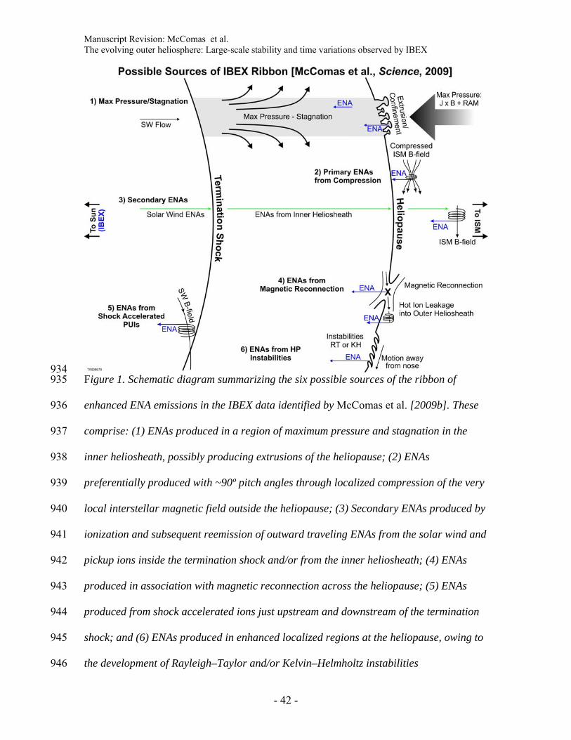
Manuscript Revision: McComas et al. The evolving outer heliosphere: Large-scale stability and time variations observed by IBEX
934 935
936
937
938
939
940
941
942
943
944
945
946
Figure 1. Schematic diagram summarizing the six possible sources of the ribbon of
enhanced ENA emissions in the IBEX data identified by McComas et al. [2009b]. These
comprise: (1) ENAs produced in a region of maximum pressure and stagnation in the
inner heliosheath, possibly producing extrusions of the heliopause; (2) ENAs
preferentially produced with ~90º pitch angles through localized compression of the very
local interstellar magnetic field outside the heliopause; (3) Secondary ENAs produced by
ionization and subsequent reemission of outward traveling ENAs from the solar wind and
pickup ions inside the termination shock and/or from the inner heliosheath; (4) ENAs
produced in association with magnetic reconnection across the heliopause; (5) ENAs
produced from shock accelerated ions just upstream and downstream of the termination
shock; and (6) ENAs produced in enhanced localized regions at the heliopause, owing to
the development of Rayleigh–Taylor and/or Kelvin–Helmholtz instabilities
- 42 -
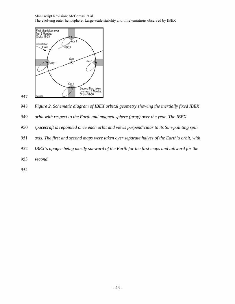
Manuscript Revision: McComas et al. The evolving outer heliosphere: Large-scale stability and time variations observed by IBEX
947
948
949
950
951
952
953
954
Figure 2. Schematic diagram of IBEX orbital geometry showing the inertially fixed IBEX
orbit with respect to the Earth and magnetosphere (gray) over the year. The IBEX
spacecraft is repointed once each orbit and views perpendicular to its Sun-pointing spin
axis. The first and second maps were taken over separate halves of the Earth’s orbit, with
IBEX’s apogee being mostly sunward of the Earth for the first maps and tailward for the
second.
- 43 -

Manuscript Revision: McComas et al. The evolving outer heliosphere: Large-scale stability and time variations observed by IBEX
955
956
957
958
959
960
961
Figure 3. IBEX-Hi observations showing the first (left) and second (right) sets of all-sky
maps in spacecraft coordinates. Both sets of maps show similar fluxes and the existence
of the ribbon of enhanced emissions. The maps are shown in Mollweide projections with
the nose of the heliosphere in the center of each map and the tail at both the far left and
far right; angles are given in ecliptic J-2000 latitude and longitude.
- 44 -

Manuscript Revision: McComas et al. The evolving outer heliosphere: Large-scale stability and time variations observed by IBEX
962
963
964
965
Figure 4. Daily (thin blue lines) and running 27-day averages (thick green lines) of solar
radiation and solar wind parameters relevant for calculating ionization rates of H ENAs
observed by IBEX (see text).
- 45 -

Manuscript Revision: McComas et al. The evolving outer heliosphere: Large-scale stability and time variations observed by IBEX
966
967
968
969
970
971
972
973
974
Figure 5. Calculated ratios of the survival probabilities of H ENAs in the second set of
sky maps divided by they survival probabilities in the first map for IBEX-Hi energy steps
2 (left) and 6 (right) as a function of spin phase vs orbit number (for the second map).
Ratios for energy steps 3-5 become progressively smaller between these two extremes.
Overall, survival probabilities are generally only a few percent different between the two
sets of maps, especially at higher energies.
- 46 -

Manuscript Revision: McComas et al. The evolving outer heliosphere: Large-scale stability and time variations observed by IBEX
975
976
977
978
979
980
981
Figure 6. Compton-Getting corrected ENA fluxes for the first (left), second (middle), and
combined (right) sets of all-sky maps from IBEX. While the second maps are somewhat
noisier, the common color bar for each energy range allows for rapid quantitative
comparison. The maps clearly show similar structures and fluxes, although some
statistically significant differences are observed.
- 47 -

Manuscript Revision: McComas et al. The evolving outer heliosphere: Large-scale stability and time variations observed by IBEX
982
983
984
985
986
987
988
Figure 7. Equirectangular projections of CG-corrected first (left) and second (middle)
sets of IBEX all-sky maps with specific contours (red and white outlines with values
indicated by arrows next to color bars) to help guide the eye. The right column of panels
show difference images where red (blue) indicates more (less) flux in the second map
compared to the first.
- 48 -
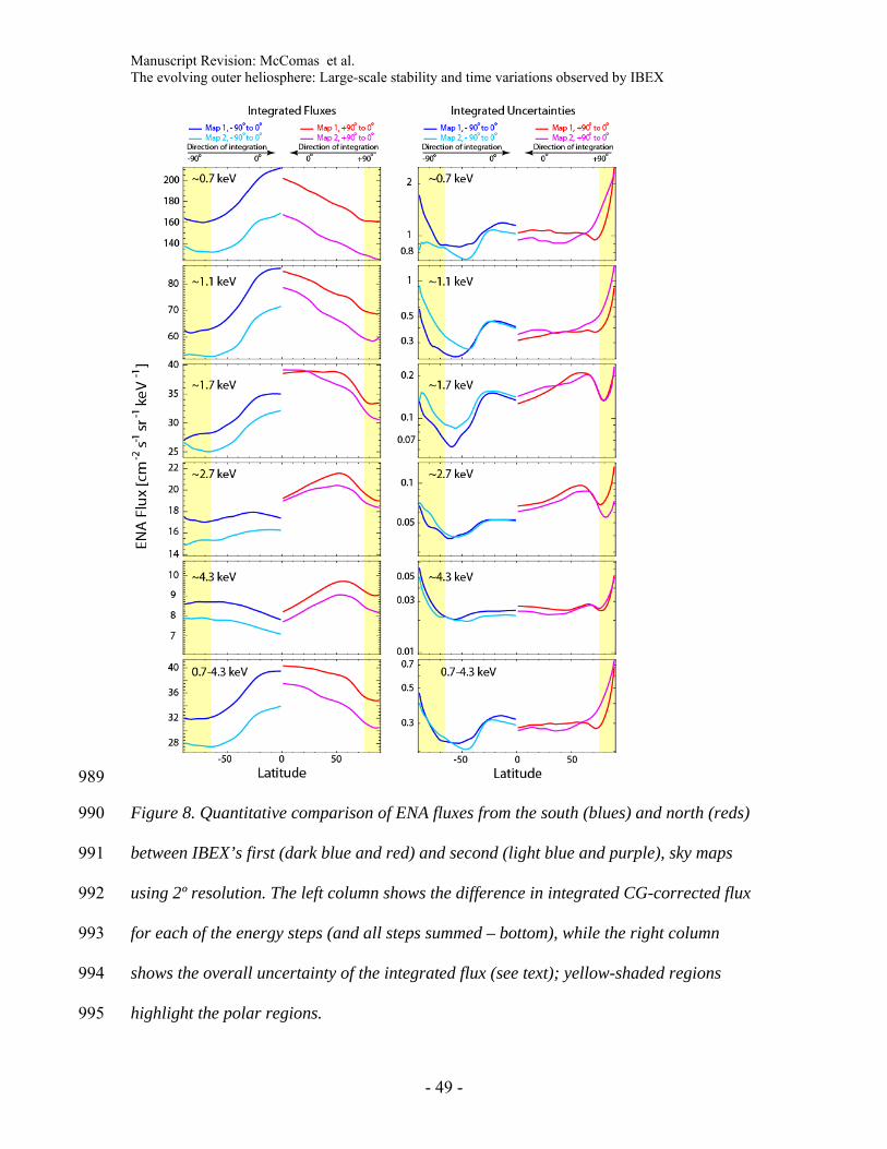
Manuscript Revision: McComas et al. The evolving outer heliosphere: Large-scale stability and time variations observed by IBEX
989
990
991
992
993
994
995
Figure 8. Quantitative comparison of ENA fluxes from the south (blues) and north (reds)
between IBEX’s first (dark blue and red) and second (light blue and purple), sky maps
using 2º resolution. The left column shows the difference in integrated CG-corrected flux
for each of the energy steps (and all steps summed – bottom), while the right column
shows the overall uncertainty of the integrated flux (see text); yellow-shaded regions
highlight the polar regions.
- 49 -

Manuscript Revision: McComas et al. The evolving outer heliosphere: Large-scale stability and time variations observed by IBEX
996
997
998
999
1000
1001
1002
Figure 9. Blow up of the knot region in the northern part of the ribbon in map 1 (top) and
2 (middle) at ~2.7 keV. The bottom panel shows the difference image of this region for all
pixels. Clearly, the knot emissions have significantly diminished (and possibly spread
out) between the two maps.
- 50 -

Manuscript Revision: McComas et al. The evolving outer heliosphere: Large-scale stability and time variations observed by IBEX
1003
1004
1005
1006
Figure 10. Energy step 3 (1.1 keV) sky map showing the three regions used for Table 2:
1) the ribbon, 2) the nose and N pole region, and 3) the tail, flanks, and south pole region.
- 51 -
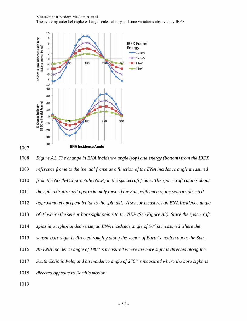
Manuscript Revision: McComas et al. The evolving outer heliosphere: Large-scale stability and time variations observed by IBEX
1007
1008
1009
1010
1011
1012
1013
1014
1015
1016
1017
1018
1019
Figure A1. The change in ENA incidence angle (top) and energy (bottom) from the IBEX
reference frame to the inertial frame as a function of the ENA incidence angle measured
from the North-Ecliptic Pole (NEP) in the spacecraft frame. The spacecraft rotates about
the spin axis directed approximately toward the Sun, with each of the sensors directed
approximately perpendicular to the spin axis. A sensor measures an ENA incidence angle
of 0° where the sensor bore sight points to the NEP (See Figure A2). Since the spacecraft
spins in a right-handed sense, an ENA incidence angle of 90° is measured where the
sensor bore sight is directed roughly along the vector of Earth’s motion about the Sun.
An ENA incidence angle of 180° is measured where the bore sight is directed along the
South-Ecliptic Pole, and an incidence angle of 270° is measured where the bore sight is
directed opposite to Earth’s motion.
- 52 -

Manuscript Revision: McComas et al. The evolving outer heliosphere: Large-scale stability and time variations observed by IBEX
1020
1021
1022
1023
1024
1025
1026
1027
1028
1029
Figure A2. The motion of Earth about the Sun makes it necessary to transform ENA
measurements from the IBEX reference frame to an inertial reference fixed with the Sun.
The geometry of this frame transformation is illustrated here. The IBEX spacecraft has
an approximately Sun-pointed spin axis, and we measure incident ENAs in the spin-plane
roughly perpendicular to the spin-axis. (Top-left) The incident ENA velocity angle, θ, is
measured relative to the NEP (X-axis) in the spin-plane as a right-handed rotation about
the Z-axis. (Top-right) The Y-axis is directed along the vector of Earth’s motion around
the Sun. (Bottom) In the spin-plane, the inertial frame ENA velocity, vi, is the sum of the
spacecraft velocity, uSC, and the measured ENA velocity, v.
- 53 -

Manuscript Revision: McComas et al. The evolving outer heliosphere: Large-scale stability and time variations observed by IBEX
1030 Table 1. Energy passbands for IBEX-Hi (qualified triple-coincidence detections) E-Step E-FW E-FWHM ENominal E+FWHM E+FW ΔE/E
[keV] [keV] [keV] [keV] [keV] FWHM2 0.35 0.52 0.71 0.95 1.23 0.60 3 0.58 0.84 1.08 1.55 1.93 0.65 4 1.07 1.36 1.85 2.50 3.02 0.62 5 1.68 1.99 2.70 3.75 4.54 0.65 6 2.57 3.13 4.09 6.00 6.93 0.70
1031
1032
Table 2. Ratios of ENA fluxes in second maps compared to first maps. Ratio of weighted fluxes (FMap-2/FMap-1) Energy
(keV) 1) Ribbon 2) Nose/N pole 3) Tail/Flanks/S pole All Sky ~0.7 0.89 ± 0.03 0.95 ± 0.03 0.67 ± 0.01 0.79± 0.01 ~1.1 0.90 ± 0.02 0.99 ± 0.02 0.79 ± 0.01 0.87± 0.01 ~1.7 0.98 ± 0.02 1.02 ± 0.02 0.92 ± 0.01 0.98± 0.01 ~2.7 0.96 ± 0.01 0.98 ± 0.01 0.96 ± 0.01 0.97± 0.01 ~4.3 0.91 ± 0.01 0.92 ± 0.01 0.92 ± 0.01 0.92± 0.01
1033
1034
Table 3. 100 AU transit times for ENAs in IBEX-Hi energy passbands. E-Step E-FW E-FWHM ENominal E+FWHM E+FW
[days] [days] [days] [days] [days] 2 668 580 469 405 356 3 519 431 380 317 284 4 382 339 290 250 227 5 305 280 240 204 185 6 247 223 195 161 150
1035
- 54 -