Time to Change.Rating Changes and Policy Implications.

Peter N. Posch∗

First Version: November 2004. This Draft: August 18, 2005

Abstract Rating agencies are often subject to the criticism of being slow in adjusting

their rating to current conditions. This paper examines the timeliness of rating changes

and identifies parameters which result in ’stickiness’ of rating actions. This stickiness is

characterized by not adjusting the rating even when market-based estimates of default

probability change. Introducing an extended econometric model of friction the migration

policy is modeled in terms of thresholds which have to be crossed by default probability

estimates before an up- or downgrade occurs. The results imply that default probability

estimates have to change by around two notches before the rating agency reacts.

Keywords: Rating Agencies, Migration Policy, Stickiness, Friction Model

JEL-Classification: C33, G20, G33

∗ Department of Finance, University of Ulm, Helmholtzstr. 18, 89081 Ulm, Germany.

eMail: pposch@uni-ulm.de

Acknowledgment I am grateful to Gunter Loffler for his encouraging support, to Manuel

Ammann and Rudiger Kiesel for valuable comments and to Moody’s Investors Service and

Moody’s KMV for providing the data. The usual disclaimer applies.

1

1 Introduction

παντα ρει και oυδεν µενει

Everything flows, nothing stands still.

(Heraklit in Plato’s Cratylus.)

Around 2,500 years ago the greek philosopher Heraklit stated that movement is the

process of nature and stability just a temporary artifact. Nowadays credit rating agencies

claim that the stability of their products is in favor of their clients and rare changes show

their ability to forecast long term credit risk. The aim of this essay is to examine when the

credit ratings change. It is thus on the ’flow’ of ratings and what causes this movement

to de- or accelerate.

One animadversion on the rating agencies is that their ratings are slow to react com-

pared to market-based measures of default risk. While manifold reasons for this slowness

are discussed in the literature there are currently only few attempts to quantify this

’stickiness’ of ratings. This paper provides a close examination on the stickiness of rat-

ing actions. Factors which influence the timeliness of a rating action are identified and

threshold parameters are estimated. These thresholds are given in units of rating-steps

and can be converted to units of a market-based risk measure. Once a threshold is crossed

the associated rating change is expected.

The policy when to change a rating is called migration policy. The direct cost of the

announcement of a rating change, e.g. publishing the new rating on the agency’s web site

or press releases, might not be very high. But the cost of adjusting and revising later

on or not adjusting at all might be immense as this affects the credibility of the rating

agency. These costs result in the stickiness of rating action as the observed migrations

differ from the expected ones.

As an example take the case of one of the biggest corporate bankruptcy in America

ever: Enron. During the year 2001 the market-based measure of the expected default

frequency published by Moody’s KMV increased from 0.35% in February to 9.88% in

November (that is a growth rate of about 2,700%) without the rating to adjust. Although

this example might sound extreme it directly leads to a question which will be answered

in this paper: To what extent has a market-based measure to imply a better/worse credit

2

quality to make the rating agency upgrade/downgrade the issuer? A desired side effect

of the knowledge of such thresholds is the anticipation a rating changes. For example

an investment manager which is restricted to investment-grade companies could easily

monitor the short-term credit risk of his investments and if it changes beyond the threshold

he can sell before the announcement.

Reasons for the stickiness of rating actions are e.g. given by Loffler (2005) and Fledelius

et al. (2004). The authors coin the term ’rating reversal avoidance’ as a reason for the

relative stability of ratings compared to market-based measures. When the rating of a

company is changed the agency wants to be quite sure that this adjustment is stable and

has not to be reversed shortly after. Thus it would be a political decision of the rating

agency to change relatively seldom in comparison to a market-based risk measure. This

migration policy dampens the volatility of the ratings and Moody’s et al. argue that a

stable rating is in favor of investors (see e.g. Cantor (2001)). But waiting too long before

adjusting is neither good for investors nor for the agency. The former might trust in the

additional information of the rating, the agency loses credibility and in the bottom line

all ratings are based on reputation (see e.g. Covitz and Harrison (2003) on the reputation

incentive). Avoidance of a rating reversal has the potential of losing reputation or in other

words each time a rating change is expected the agency has to balance the gains of a stable

rating with the losses from being ex post incredible. This optimization problem can be

expressed in terms of transaction costs given above and instead of calling a migration

policy ’slow’ it is more appropriate to think in terms of ’stickiness’. A rating action might

not be taken even if a change in the markets valuation of credit quality implies so. Such

a migration policy would be sticky since the rating does not adjust. Rating stability and

reputation incentives thus result in stylized facts such as the rating drift, i.e. it is more

probable to see a subsequent rating change in the same than in the opposite direction.

There is a branch of literature which is related to the questions posed in this paper.

Loffler (2005) uses simulations and Altman and Rijken (2004) use actual rating data in an

empirical approach to ascribe the stylized facts to the migration policy. The latter authors

compare a constructed ’agency’-rating with a benchmark market-based rating using the

methodology of Shumway (2001) and the variables given by Altman (1968). Through

3

simulations they conclude that a rating change is triggered if the actual through-the-cycle

credit quality exceeds 1.25 notch steps of the average credit quality for a given rating

class. Kavvathas (2000) examines to which extend the rating changes depend on the

current business cycle. His methodology of the ordered probit analysis is also used by

Nickell et al. (2000) to investigate sector and cyclical effects and by Blume et al. (1998)

and Jorion et al. (2004) to answer the question whether the rating agencies policy has

changed during the 1990s.

This paper introduces a general methodology which can be applied to any kind of price

stickiness. Extending ’models of friction’, which are generalizations of the Tobit-Model

by Tobin (1958), thresholds which have to be exceeded to observe a rating change are

estimated. Using a comprehensive data set the results obtained by Altman and Rijken

(2004) and Loffler (2005) are quite verified by additionally providing a closer insight into

the timeliness of rating action. The migration policy is estimated in units of threshold-

levels which have to be crossed to observe a rating change. For example if the two-year

change of a market-based measure exceeds -2 notches then this issuer is upgraded. If this

change is 1.6 percentage points a downgrade is observed and if the change is between these

numbers the rating does not react but is subject to stickiness. The unobserved (latent)

rating changes without the presence of such transaction cost can be predicted within the

models.

The first economic application of the friction models is given by Rosett (1959). The

author extends the Tobit model to estimate the change of portfolio composition in response

to changes in yields. His model can be described as a double censored tobit model.

This model is further extended by Dagenais (1969) and refined by Dagenais (1975) to

include fixed costs. Applications of these models include the estimation of central bank

intervention by Almekinders and Eijffinger (1996) or Asano (2002) who examines the

effects of costly reversible investment.

This paper extends the methodology of frictional models with respect to the use in

panels and variation in the coefficient estimates for the negative and positive parts of

the model. In contrast to the current literature, which mainly uses static models with

constant cut points, the identification of the driving factors of the rating stickiness leads

4

to a more detailed insight into the rating methodology itself. The quantification of the

impact of these factors sharpens these results.

The remainder of this paper is organized as follows. Section 2 describes the data set.

Section 3 introduces the friction models, while section 4 introduces the variables used in

the analysis. Section 5 gives the results of the empirical analysis. Section 6 summarizes

and draws a conclusion.

2 Data Set

In the analyses I use a comprehensive data set which contains monthly information on

Moody’s long-term ratings and a market-based default risk measure by Moody’s KMV

(’MKVM’, hereafter). The data set consists of 4,023 US and Non-US corporate issuers

and covers the period from January 1980 to April 2005. Figure 1 shows the evolution

of issuers in the data set. In April 1982 Moody’s refined its rating system and added

new rating modifiers (the ’alphanumerical’ ratings, such as Aaa3). Because the focus of

this paper is on the rating migration policy and the refinement itself is not a migration

triggered by a change in the issuers credit quality I start in January 1983 for the analysis

below. Furthermore I exclude migrations to default. A rating change to the default

category and changes within default cannot be considered as a political migration as this

decision is forced exogenously rather than influenced by a rating committee.1

The variables used in the regressions are based on MKMV’s expected default frequency

(EDF, hereafter) and Moody’s issuer rating. The EDF reflects a point-in-time (PIT,

hereafter) default frequency as they are based on current market measures, while the

issuer rating of Moody’s and other rating agencies reflects (more or less) a through-the-

cycle (TTC, hereafter) approach (see Loffler (2004) and the literature cited there).

Recent research by Hamilton (2004) implies that short-term EDF changes has impact

on secondary rating information such as outlooks and watch-lists. For a subset of this

data set staring in September 1991, outlook and watchlist data is available. In this subset

adjusted ratings (ADJRAT, hereafter) are estimated using the methodology of Hamilton

1Sensitivity analysis including defaults show no qualitative change in the results which could be due

to the relatively small proportion of defaulters in the data set.

5

(2004), p. 11. The adjustments are symmetric for positive and negative conditions where

reviews adjust for two notches and outlooks for one notch. For example an issuer with a

rating of B2 and a positive outlook has an adjusted rating of B1, while a negative review

would results in an adjusted rating of Caa. Overall there are 3,462 issuer with available

outlook information.

The issuer rating is converted to numerical scale with Aaa (∼ 1) to C (∼ 21) (RAT,

hereafter). Table 6 shows descriptive statistics of each rating category.2

For similarity of scaling the ordinal ratings can further be transformed to a probability

of default (PD, hereafter). This transformation can be done in different ways leading to

different implications. First, one could use idealized PDs as e.g. published by Moody’s.

The idealized PDs sharpen the TTC approach of the rating agencies as they do not

react to any differences over time. In contrast, the mapping of the ratings to their PDs

can be done using the (ex post) yearly transition matrices. This approach incorporates

information on macroeconomic changes over the time and thus reduces the TTC nature

of the ratings. Between these two procedures is the mapping of ratings to the PDs of a

transition matrix over the whole period of the data set. This transition matrix can either

be obtained from publications of the major credit agencies or be calculated within the

data set. As the main purpose of this paper is to shed light to the rating black box it is

reasonable to model in line with the agencies’ predictions I use idealized PDs to transform

the ratings (PDRAT, hereafter), see table 8 for details.

The MKMV expected default frequency (EDF) estimates a one-year probability of

default based on market measures such as balance sheet data, equity volatility and equity

value. This cardinal measure of the PD is based on the ’distance to default (DD)’ given

by equation 1, where A is the current market value of the company’s assets, DPT is the

default point, µA the expected market return to the assets and σA the volatility of ln(A).

DD =ln(A/DPT ) + (µ− 1/2 · σ2)(T − t)

σ√

T − t(1)

In the approach of Merton (1974) the PD is given by applying the standard normal

2Without the alphanumerical modifiers the conversion to letter grade ratings results in eight rating

categories. The specification of the letter grade ratings has been tested in each of the specification given

in section 5 below and did not yield qualitatively different results. Details are available upon request.

6

cumulative distribution function to the distance to default: PD = Φ(−DD). MKMV, in

contrast, calculates the EDF by calibrating the distance to default to empirical (historical)

default rates, resulting in a minimal EDF of 0.02% and a maximal EDF of 20%. Kealhofer

(2003) shows that the empirical distribution function used by MKMV is not normal, but

has much wider tails. For example a DD around 4 maps to a EDF of around 11 to 6

basis points. The equivalent probability using the normal distribution Φ is virtually zero.

Using a logarithmic transformation, which results in wider tails, the PD is different from

zero. Thus a logarithmic transformation preserves the information of the tails, i.e. it can

discriminate among issuers with very high or very low PD. Througout this paper I will use

log-EDFs instead of level-EDFs, if not stated otherwise. Whenever certain EDF values

are quoted they refer, however, to the level of the EDFs. Figure 2 shows the mean and

median of the EDF over time for all issuers and issuers with investment-grade rating.

There are two things notable on these variables. Firstly in practice the rating is not

a pure through-the-cylce rating and the EDF is not a pure point-in-time estimate of the

credit quality. Both measures are noisy. The noise in the EDFs can lead to an expected

rating change even if the current rating is still appropriate.

Secondly - and abstracting from the first point - the rating changes should not only

react to changes in the level of the EDF, but also to the percentage changes of the EDF,

i.e. impact on the rating should differ across the EDF spectrum. E.g. an EDF change

from 0.04% to 0.14% should be weighted differently to a EDF change from 0.3% to 0.4%.

The percentage change in the former case is 250% while the latter example has a growth

rate of 33.3%. To capture this effect it is appropriate to use percentage changes, i.e.

changes of the log-EDFs, instead of changes in the levels.

3 Methodology

The rating policy of volatility aversion and the methodology of attempting to look through

the cycle are major reasons for observing stickiness in rating changes. The econometric

approach used here estimates the observed rating changes as a function of the observed

change of the current creditworthiness measured by the expected default frequency. The

model is estimated by three equations each describing a different rating behaviour. When

7

the change of the EDF and the following rating change are moving in the same direction,

i.e. an upgrade is observed in response to a decrease of the EDF or an increase in the

EDF is followed by a downgrade, we are outside the frictional part of the model. But

if the rating remains unchanged even if the EDF declines/raises the rating is subject to

stickiness. To put it the other way around the models quantify the question to what

extend the independent variable has to change to observe a change of the dependent

variable, i.e. the rating.

3.1 Friction Models

Let RAT ∗i,t be the expected but unobserved (latent) rating for company i at time t. This is

the rating which would be observed if the rating was not subject to stickiness or friction.In

a frictionless rating system the actual rating RATi,t thus equals the expected rating and

analogous for their changes: ∆RATi,t = ∆RAT ∗i,t. Let the operator ∆n denote the n-th

difference, i.e. ∆nx := xt − xt−n, where the subscript is suppressed when denoting any

(non-specific) difference.

Independently of the migration policy the expected (latent) rating change ∆RAT ∗i,t

can be modeled by a vector X = (x1 x2 ... xk) of k exogenous variables as shown by

equation (2).

∆RAT ∗it =

k∑i=1

βixit + εit = β′X + εit (2)

Now the actual, i.e. observed, change in the rating is a function of the expected rating

change according to ∆RATi,t = τ(∆RAT ∗it). The function τ(·) maps the unobserved latent

variable RAT ∗ to the observed variable RAT via a nonlinear rule. In the frictionless case

described above τ would equal the identity function since there is no rating policy present.

To introduce rating friction I discuss two functions τ(·), where the friction models used

here are generalizations of the Tobit-model by Tobin (1958) by Rosett (1959), Dagenais

(1969) and Dagenais (1975).3

3For a ’classical’ Tobin model τ(·) is given by ∆RAT =

∆RAT ∗ ,∆RAT ∗ < cl,∆RAT ∗ > ch

0 , cl ≤ ∆RAT ∗ ≤ ch

.

8

Consider a rating decision based on the change of the EDF in the last six months. If

the EDF decreased by less than what a notch implies the rating would remain unchanged

unless other information presume the converse and are weighted respectively. But even

if the EDF decrease is greater than that a rating change (upgrade in this case) is still

unlikely since e.g. the time period in which the company’s credit quality increased is very

short and the stability of this improvement is uncertain. The analogous argument holds

for an observed increase of the EDF. An econometrician thus could (and does) observe

no rating changes when a rating-change would be expected given the observed change of

a suitable proxy. But why is no rating change observed even if long-term proxies would

expect a reaction? An economic interpretation in terms of transaction cost is that a

rating-change is costly reversible, i.e. a rating reversal is possible but costly e.g. in terms

of reputational losses. These reputational losses are not constant but rather variable. E.g.

a downgrade from BBB to BB followed by a reversal is probably more severe than from

BB to B and back to BB.

The cost of the rating change announcement itself, i.e. the publication of the new

rating on the internet, press-notes etc., is considered marginal. This assumption is tested

using a generalized model and verified empirically in section 5.

Let α1 < 0 denote a (desired) decrease and α2 > 0 an increase in ∆RAT ∗. The fixed

costs are given by γ1 ≤ 0 and γ2 ≥ 0. The actual (observed) rating change under friction

is given by equation (3) below.

∆RATt =

∆RAT ∗

t − α1 + γ1 , ∆RAT ∗t < α1 (L)-Area

0 , α1 ≤ ∆RAT ∗t ≤ α2 (F)-Area

∆RAT ∗t − α2 + γ2 , α2 < ∆RAT ∗

t (U)-Area

(3)

Each line of equation (3) corresponds to an area of figure 3, where the left graph shows an

idealized graphical representation of the friction model without fixed costs (γ1 = γ2 = 0),

while the right graph shows the addition of vertical friction. The areas refer to the position

of the derived function, where L denotes the lower part, F the friction area and U the

upper part. Note that the slope coefficients in figure 3 are equal for both the lower and

the upper part. I extend this restriction by generalizing the equations to include different

9

slope coefficients.4

Note that in figure 3 the x-axis has values of ∆RAT ∗ whose expectational value is

(according to equation (2)) β ′X. The threshold-parameters αi are thus estimated in units

of the dependent variable. Consider e.g. the model ∆RAT ∗ = β1 ·∆EDF +ε and suppose

that the coefficient estimator for the only exogenous variable is equal to 30, i.e. β1 = 30

and the threshold-parameters are α1 = −0.5 and α2 = 0.4. Then the model tells that if

∆RAT ∗ is between −0.5 and 0.4 we are in the frictional part (area F in equation (3)).

A more commonly statement would sound like ’for EDF changes between -1.6pp and

1.3pp we do not observe any rating change’. Converting these thresholds from units of

∆RAT ∗ to units of the exogenous variable is straightforward. What equation (3) tells is

’if ∆RAT ∗ is smaller than α2 = 0.4 but bigger than α1 = −0.5 we observe friction’. Since

the estimators are unbiased that is equivalent to α∆EDF1 = −0.016 < ∆EDF < α∆EDF

2 =

0.013 as obtained by solving equation (2) for ∆EDF . Extending the results to cases

with more than two exogenous variables is possible using E[∆RAT ∗] =∑

j βk · E[xk].

Solving this equation for any variable xl gives the threshold parameters in units of xl:

αxlj := (αj −

∑k 6=l βk · E[xk])/(βl) for l 6= k , j = 1, 2. Note that this procedure is

appropriate only in absence of interaction terms. When interaction terms are included

the correlation of the interacting variables would has to be accounted for.

An important extension of the friction model is the inclusion of variable threshold

parameters. Instead of estimating αj as constants one can include variables xαj

k . Of

course this results in a distribution of thresholds rather than constants. In the following

analysis the means of this distribution is reported whenever the threshold model includes

variables.

In every model εi,t is a serially uncorrelated, homoskedastic error term with mean

zero and time-constant variance. To control for issuer-specific heterogeneity I use the

Huber/White-sandwich (HWS) estimator of variance which result in cluster-robust stan-

dard deviations. This estimator’s origin is Huber (1967) and White (1980) whereas the

4Note that equation (2) does not allow for a constant β0. In this model the inclusion of a constant

would shift the threshold parameters αi. To see that elongate the curves of the areas (L) and (U) in figure

3 toward the vertical axis. Thus the inclusion of a constant does not change the level of the estimated

threshold.

10

term ’sandwich’ refers to the mathematical form of estimation. The standard HWS as-

sumes independence of observations itself, but when specifying clusters, such as issuers,

the independence of clusters is assumed instead. This leads to a straightforward modifi-

cation of HWS to deal with clusters, see e.g. Wooldridge (2002) for details.The Maximum

Likelihood function for the friction model of equation (3) is derived in the appendix.

4 Variable Selection

The model introduced in the previous section and the results obtained in the ongoing

section 5 are based on the rating as Moody’s prediction of the long-term credit quality

and the EDF as a market-based short-term measurement of the probability of default.

The information contained in these measures has to be further extracted to gain detailed

insights into the factors which trigger a rating migration. In fact the friction model needs

the specification of two models. Firstly, the model of the latent rating change ∆RAT ∗,

which is equivalent to specifying the ’true’, but unobservable, credit quality process. And

secondly, the specification of the variables which trigger a rating change, i.e. the threshold

models αi.

Concerning the ratings the theoretical literature dealing with the probability of mi-

grating from one rating to another assume these probabilities to be markovian. Empirical

work (e.g. Lando and Skodeberg (2002)) shows that this probability depends on the path

of the rating. Abstracting from cyclical effects there is evidence that the time spent in

a given rating class as well as the direction from which the current rating was achieved,

i.e. downgrade or upgrade, influences the probability of further rating migration. The

first observation of this behaviour is given by Altman and Kao (1992a), Altman and Kao

(1992b) and Lucas and Lonski (1992). These authors coin the term ’rating drift’ and al-

though the exact definition differ within the literature this stylized fact is typically based

on proportions of downgrades to upgrades (or vice versa) within or across rating classes.5

Recent papers include Kavvathas (2000), Lando and Skodeberg (2002) and Fledelius et al.

(2004) which examine whether the history of rating migration influences the current tran-

5Fledelius et al. (2004) point out it is consistent with markovian behaviour to have a larger proportion

of either downgrades or upgrades from a given rating class.

11

sition probability and find similar results as Altman and Kao (1992a): Downgrades are

autocorrelated, i.e. a downgrade is more likely to be followed by another downgrade than

an upgrade. For upgrades this serial dependence is less pronounced, i.e. statistically not

as significant as the downgrade momentum.

One straightforward way to control for durational effects is to measure the months

spent in a rating class starting with the last rating change.6 This definition, however, is

collinear with the endogenous variable and thus cannot be used as an exogenous variable in

the models specification. In lieu thereof the durational effect is controlled by the following

variable.

One problem when estimating changes of agency ratings is the methodology of buck-

eting. Issuers with different point-in-time credit quality are coalesced in the same bucket.

And since this assembly changes over the time, the distance of each issuers current point-

in-time credit quality to the ’typical’ quality in his current rating class accounts for both

the durational effects and the relativeness of a rating system. This variable is denoted

by BMEDIAN − EDF . Note that this variable also controlls for the effect of rating

reversal avoidance, see Loffler (2005) for details. Low values of this variable indicate that

the issuer’s current credit quality is in line with the other issuers rated equally well, while

high values indicate a difference between the market measure of credit risk of this issuer

with the typical company rated this grade. The sign of the variable gives the distance of

distortion from the median.

Using the transformed ratings and EDF data I control for the distance between the

PD currently implied by the rating and the EDF. Since KMV considers its EDFs to give a

1-year PD I use the one year horizon denoted by PDRAT1. The difference of the one year

implied PD and the EDF (PDRAT1−EDF ) can be interpreted as follows. If the rating

has been very stable over a long period of time, i.e. the ratings duration is very high, but

the current difference between the implied PD and the EDF is high and negative, i.e. the

EDF is higher than the agencies’ suggestion, then the probability of a rating change is

lower if the agency follow a TTC approach than a PIT approach. The rationale is that

6If information is missing in the data set, the duration is stopped at the missing value and increased

if the next rating is the same and else restarted. This leads to a ’minimum duration’ definition in the

sense that an issuer’s rating stayed at least ’duration’-month in the given rating class.

12

the agencies belief about the issuers willingness to increase its creditworthiness within a

short period of time is strengthened by past experience captured in the duration. This

behavior is conditional on the current rating level since a long duration in the lower non-

investment grades should result in a higher transition probability than within the higher

investment grades.

Furthermore the volatility of the change in EDFs is estimated (V OLA := σ(∆EDF )).

This term controls for the precision of the markets view on the company’s credit quality.

The higher the volatility the more unconfident the market. The expected sign of this

variable is negative. For an desired upgrade this is because high volatility is opposed to

the higher stability implied by a higher rating grade. While the same arguments justifies

a quick downgrade (recall that a downgrade is denoted by a negative rating change).

As stated above the EDF is a noisy measure for the point-in-time credit quality of

an issuer. Likewise any other noisy measures this leads to a decline in the precision

of the estimates. Assuming that the EDF can be decomposed in a cyclical component

EDF cycle and a trend component EDF trend, Leser (1961) proposes a technique which

is later improved by and named after Hodrick and Prescott (1997): the HP-filter. The

original series EDFit = EDF trendit + EDF cycle

it is decomposed into its parts by solving the

following optimization problem:

minEDF trend

it

T∑t=1

((EDFit−EDF trendit ))2+λ

((EDF trend

i,t+1 − EDF trendit )− (EDF trend

it − EDF trendi,t−1 )

)2

Here, λ is a penalty parameter which is set a priori. This parameter penalizes the

roughness of the original series. Higher values of λ lead to a smoother cyclical component.7

In the analysis below I set λ to the commonly used value for monthly data of 14,400. As

a comparison I report results for λ = 500, 000 whenever the conclusions change.

The overall correlation of Moody’s issuer rating when using λ = 14, 400 is 70% (72%

for λ = 500, 000), while using the EDF the correlation is at 66%. Thus this smoothing

parameter is appropriate in this setting. The filter is estimated per issuer on the loga-

rithms of the EDF. Figure 4 gives a graphical representation of the filter for an arbitrary

7Note that in the limit λ → 0 the trend component approaches the original series, while in the limit

λ →∞ this component approaches linearity. For a more detailed discussion see e.g. Schlicht (2004)

13

issuer.

The trend of the EDF (HPEDF, hereafter) is (by construction) lacking any temporary

fluctuations. Since the filter is forward looking it proxies a rating agency’s view of the

point-in-time measure.

Furthermore I use a dummy variables for investment grade rated issuers (INV EST ).

This dummy is equal to one if the rating is between Aaa ∼ 1 and Baa3∼ 10 and zero for

the speculative grades (Ba1∼ 11 to Caa3∼ 21). I controll for recession periods according

to the National Bureau of Economic Research (NBER), where the first recession during

this data set is R1 for July 1990 to March 1991 and the second recession period R2 for

March 2001 to November 2001.8 Both recession periods are accumulated in the dummy

variable RECESSION .

5 Results

In this section both the friction model and its generalization are estimated. The general

friction model with γ1 6= 0 , γ2 6= 0 (GFM) is used to analyze the height of fixed costs

of rating changes. All results are controlled for the investment-grade boundary yielding

estimates for each subset and the whole data set. Convergence of the maximum likelihood

was usually achieved after less than forty iterations, where the tolerance level of likelihood

estimation is set at 10−7.

5.1 Basic Model

In the initial setting I model yearly rating changes (∆12RAT ) on yearly percentage changes

of the expected default frequency (∆12EDF ). Unless stated otherwise non-overlapping

time periods with the months of January, June and December are used. Sensitivity

analysis show that the choice of the period is not crucial (see the appendix for details).

Table 6 shows the results for the initial setting, where panel (A) gives the results for the

friction model with the restriction of equal slope coefficients for the upgrade (L-area) and

downgrade (U-area) while panel (B) releases this constraint. Both settings are estimated

8See http://www.nber.org/cycles.html.

14

with the full data set as well as for investment-grade rated issuer and speculative-grade

rated issuer only.

In both specification the hypothesis that rating changes are not subject to fixed or

menu costs cannot be rejected. The fixed costs parameters γ1 for the upgrade-section

(the L-Area in figure 3) and γ2 for the downgrade-section (the U-area) are either not

significantly different from zero or smaller than |1 · 10−9|. These parameters capture

friction due to such costs as announcement of the rating change itself. Such costs are

presumably very low if not zero. Note that this does neither imply that there are time-

varying fixed costs nor that the rating process itself does not contain fixed costs, but

solely that the decision whether the agency announces a rating change is not subject to

an fixed (constant) amount.

All other coefficients are highly significant. The restricted setting of panel (A) shows

estimates which are between those obtained by releasing this restriction, e.g. the coeffi-

cient of the LNEDF change (∆12EDF ) in the full model is 0.663 when imposing equality.

This coefficient splits to a value of 0.401 for upgrades and 0.818 for downgrades when

using the generalized specification. These coefficients specify the change of the expected

rating ∆RAT ∗ in response to an observed percentage change of the EDF. The inverse of

this coefficients gives the percentage EDF change needed for an one-notch change of the

expected rating. In this very case this means that if ∆12EDF = 1/0.663 = ±1.508 then

the expected rating changes by ± one notch. This is equivalent to a percentage change

in the EDF of exp(1.508)− 1 = 351%.

Although this figure seems quite high at first, it is not uncommonly observed in this

data set and the initial example of Enron is only one case in which even higher percentage

changes where needed to trigger a rating change. For downgrades this number is within

the upper 95% of the distribution. The 99% quantile is at a percentage change of 1,275%,

while for upgrades the 1% quantile value is at a percentage change of 99%. For the panel

(B) this picture sharpens. While changes of the EDF exceeding the one-notch threshold

are observed quite often for downgrades, the upgrade part is observed seldom. Note,

however, that this calculation assumes that the error term is virtually zero.

The threshold parameter vary between -4.5 to -3.6 notches for upgrades and 3.0 to 3.6

15

for downgrades, depending on the specification and sample used. The thresholds in panel

(B) are smaller (in absolute) values compared to panel (A). In addition with the higher

Log-Likelihood this indicates a better fit when not restriction the slope coefficients. The

threshold parameters implicate that a decline of more than 3 notches of the latent credit

quality triggers a downgrade. For upgrades this unobserved credit quality has to raise by

more than 3.6 notches to observe an upgrade.

What is the reason for observing such a low frequency of upgrades using this threshold?

One technical reason is the lower proportion of upgrades compared to downgrades and

no-rating changes. In this setting there are 8.08% upgrades, 66.22% no rating changes and

14.53% downgrades observed. An economic reason lies in the variables used. A one-year

EDF change might be a reasonable variable to predict downgrades, but a too short time

period for predicting any upgrade. When a rating agency upgrades a company the rating

aversal avoidance is more severe. Firstly the better credit quality reflected by an EDF

decrease is more fragile than the decline of credit quality reflected by an increase in the

EDF. As the agency attempts to provide a through-the-cycle rating this short-term credit

quality increase may not be enough to alter the business cycle the company is in. The

reason why the downgrade thresholds are on a reasonable level is that, depending on the

position of the business cycle and macroeconomic conditions, a one year increase of the

EDF might be the beginning of some trouble. To put it in other words: Being temporarily

better does not imply being good, but being temporarily worse is a smoking gun.

A further reason is due to the transaction costs of the rating agency. As assumed

and verified empirically the fixed costs are marginal. The variable costs for doing a

rating change and the possibility of reverting that change afterward are summarized in

the reputational losses. It is likely that these costs vary with the last rating of a company

before an expected change. When upgrading e.g. from speculative- to investment-grade

and reverting that decision will result in higher reputation costs than upgrading from

e.g. CC to C and downgrading again. This behavior could be more pronounced for

upgrades than for downgrades. Since an upgrade lowers the company’s cost of financing

and simplifies the access to debt resources. In presence of investment restrictions the

demand for a long-term stable rating change is even higher. Concluding the initial model

16

is sufficient to capture downgrade stickiness, but does not seem to be adequate for upgrade

stickiness, which is partly due to the lower proportion of upgrades in the data set.

5.1.1 Thresholds over time and horizons

Closely connected with these arguments is the specification of the latent rating change

∆RAT ∗. Recall that the latent credit quality process is modeled by the percentage change

of the EDF. The EDF measures the current-conditions and does not reflect the through-

the-cycle methodology of an agency rating. Nor the process of bucketing issuers with

different point-in-time credit risk into one rating bucket is modeled. Furthermore the

threshold are estimated over a time period of 20 years and over the whole rating spectrum.

They thus mark a maximum threshold which certainly triggers a rating event for any

rating class and any point in time. Before extending the models specification the evolution

of thresholds over time refines the results obtained so far. For that purpose I include

dummy variables for each year. Using one-year rating changes dummies for the first

year 1983 and the last year 2005 are excluded. For the remaining years figure 5 shows

the result for the model estimated in panel (B) in table 6 above with 95% confidence

intervals. The mean thresholds over all years are identical to the thresholds estimated

over the whole period. The volatility over time is 0.31 notches for upgrades and 0.60

notches for downgrades implicating that the fluctuation over the years has more impact

on the downgrades.

While the thresholds are relatively stable over the years, the question arises whether

the specification of the time-horizon is robust. When the EDF measures the current-

condition of the credit quality, but the ratings react only to persistent changes, the changes

in the latent rating might not go back long enough to capture the triggering current-

condition change. Connected with this question is the robustness of the dependent variable

specification. In this initial setting I used the one-year rating change (∆12RAT ), but how

do thresholds change with a longer/shorter horizon? Since it can take some month from

the rating decision to actually changing the rating, it could be that the current EDF

changes do not capture the decision. If so either longer time horizon for the EDF change

or EDF changes some months ago would be the appropriate candidate for measuring

17

the rating trigger. To answer these question I start with a rating change of six month

(∆6RAT ) explained by a six month change of the EDF , which is increased successively by

six month. Then I increase the dependent variable by six month which is again explained

by increasing changes of the EDF . The final specification tested is the 30 month rating

change by the 60 month change of the EDF . Figure 6 shows the results for the threshold

level.

The thresholds are very stable for each specification of the independent variable. In

fact, the volatility of all parameter is very low (between 0.01 and 0.05). Thus a longer

time horizon of the latent credit quality does not alter the results. An interpretation of

this stability is that the rating changes within one period, e.g. one-year, can be explained

in terms of a friction model with latent changes during the same period. Put the other

way around, longer changes of the EDF do not lower the thresholds set by the agency and

thus do not fasten a rating change. The same results is obtained when holding the time-

horizon of the changes constant but adding successively lags to the independent variable,

i.e. using the one-year EDF change from six months ago.

Comparing the specifications of the dependent variable among each other shows that

the longer the time horizon the smaller the thresholds which have to be exceeded to

trigger an observed rating change. The decrease of the threshold is most pronounced

when switching from a six-month rating change to a one-year rating change. Continuing to

increase the time length declines the changes of the thresholds. In fact the two-year rating

change and the 2.5-year rating change specification are both within a 95% confidence

band. An economic reason would be the through-the-cycle methodology. During two

year most of temporary conditions should have changed and this should be reflected both

in a (permanent) shift of the EDF and a change of the rating. In fact switching form

one-year rating changes to two-year rating changes almost doubles the mean of these

variables.

5.1.2 Quantification of the estimations bias

The previous sensitivity analysis indicates two further examination. Firstly, the model

with two-year changes should accompany the initial setting. Secondly the impact of the

18

through-the-cycle methodology on the estimates has to be captured, before a consistent

interpretation of the threshold parameters is appropriate.

To assess the impact of the through-the-cycle methodology on the estimation of the

thresholds I conduct the following simulation study. Based on the trend of the EDF

obtained by the Hodrick/Prescott-filter (HPEDF ) - as described in section 4 - I construct

a benchmark rating system (HPRAT , hereafter). In every year I obtain the percentage

of observation in each rating category. Using the density of HPEDF new rating classes

are assign according to the observed frequency. For example, in 1983 there are 2.6% Aaa

rated company-month. The lowest 2.6% of the HPEDF are thus assign to the rating-class

HPRAT = 1. This methodology ensures that the constructed rating depends only on

the number of observation and the trend of the EDF. The mean of the construced rating

and the original rating do not differ significantly, but the former’s volatility is lower. Note

that this constructed rating is a pure through-the-cycle rating with respect to the EDF

by construction. However, ratings are still assigned to buckets of issuers. It is thus not

free of bucketing and effects caused by this method. Such effects are controlled for in the

following section using interaction terms.

Figure 7 shows an example of Moody’s rating, the constructed rating and the EDF

trend for an arbitrary issuer and table 3 gives the results for the HPRAT as dependent

variable for the one-year and two-year specification.

The thresholds obtained using the simulated rating vary between 0.5 and 1 notches

for both upgrades and downgrades. They are higher for upgrades of speculative grade

companies and lower for downgrades in this subset. Switching the specification from one-

year to two-year changes has only marginal effect of about 0.1 notches. Using the trend

of the EDF with higher values of the smoothing parameter λ (see section 4 for details)

increases these numbers by 0.3 to 0.5 notches.

Overall when interpreting the results of the initial model the through-the-cycle

methodology and the noise due to bucketing account up to 1.5 notches. Assuming that

these effect are additive, the estimated notches have to be corrected by the thresholds in

table 3.

The last robustness check before extending the models specification is the assumption

19

of the error term. The friction models (FM) assume that the error term εi,t ∼ iid N(0, σ2),

i.e. that there is a homogeneous variance over time. While I assume that this assumption

holds I will now extend the models to control for time-varying variance. Time-varying

variance is examined on a two-year basis, i.e. I assume that the variance does not differ

significantly within each two-year block: εi,t ∼ iid N(0, σ2y) with y ∈ {[i, i + 2], i =

1, 3, 5, ...}. In addition to this procedure I control both for panel-unit heteroskedasticity

and time-varying variances. The choice of the tree-year block is not arbitrary but given

by the independent variable used. In the specification above the two-year EDF change

forces a data length of more than one year since at the end of the first year there is only

one observation. The variance estimation is done separately for the three subsamples

(whole data set, investment and speculative grade). The results do not differ significantly

from the setting with time homogeneous variance. It can thus be concluded that the

assumption of a time-constant error term variance is not crucial in this setting.9

The ongoing extension of the models specifications is based on the findings obtained

so far. Firstly, the thresholds are relatively stable over time and the thresholds estimated

over the whole time period approaches the mean of the thresholds estimated in every

year. Secondly, the specification of the time-horizon of the latent rating change is not

crucial. The most obvious choice is thus using the same horizon for the dependent and

the independent variable. Thirdly, the threshold parameter are decreasing (in absolute

values) with longer rating changes. This process diminishes with more than two-year

rating changes. Fourthly, the effect of the through-the-cycle and bucketing methodology

is about 0.5 notches for upgrades and 0.8 notches for downgrades. These values are stable

over different specifications. And lastly, the assumption concerning the error term are not

crucial.

5.2 Factors of Stickiness

While the initial setting revealed the robustness of specification of the latent credit quality

process, the impact of variables on the migration policy is yet unclear. In the remainder

of this paper I redefine the models specification using the additional variables described

9Detailed results are available upon request.

20

in section 4 to explain their impact on the stickiness. Further I include interaction terms

of these variable within the latent rating model.10To compare the results with the former

specifications I present the mean-slope coefficient of the latent model and the mean-

threshold for each of the following models.

Table 6 shows the details for the extended model, using variable threshold parameter

and interaction terms. Starting with the results for the latent model, for upgrades the

interaction of the PDRAT − EDF variable is positive, i.e. if the current rating’s PD

is higher than the EDF the slope becomes steeper and a upgrade is triggered by less

intensive changes in the EDF. The volatility of the EDF changes is negative for the one-

year setting (panel (A)) and positive for the two-year setting. Since the coefficient is not

very high compared to the other interaction terms, the impact is not that strong. The

direction although is that higher volatility results in flatter upgrade responses over the

one-year horizon and steeper responses in the two-year setting. The final interaction term

is the difference of the bucket median and the EDF. Here the effect is negative, i.e. if

50% of all issuers have a higher EDF (BMEDIAN −EDF > 0) the upgrade response is

flatter. That means the more an issuer moves away from the buckets median, the flatter

is the rating response. One reason for this observation might be the avoidance of rating

reversals. If an issuers expected rating differs only by a small proportion from the current

rating, a rating change should be unlikely and if triggered the new rating will not differ

much from the old one. For the downgrade specification all implications are the same

since the coefficients are in the same direction. The mean slope coefficients do not differ

much from the ones estimated without interaction terms (see table 6).

Considering the threshold specification and starting with the time dummy

RECESSION it can be concluded that during a recession period upgrade thresholds

become larger, i.e. higher changes of the latent credit risk are needed to trigger an up-

grade. And downgrade thresholds become smaller during a recession. These effects are

quantified by the coefficient estimators, i.e. in the one-year setting of panel (A) a re-

cession increases the upgrade threshold by 0.375 notches and decreases the downgrade

threshold by 0.394 notches. The effect of the recession on the two-year changes is a bit

10Note that all these variables are based on the EDF. The inclusion of rating based variables, such as

the duration measured in month will result in collinearity of the endogenous and exogenous variable.

21

less pronounced.

The volatility of the EDFs decrease the downgrade threshold, i.e. the more volatile the

EDF the more likely is a downgrade. This effect is stronger for speculative-grade issuers.

For upgrades the effect is mostly not significant. The PDRAT − EDF variable gives

a mixed picture. The coefficients are negative for upgrades, i.e. if the rating’s implied

PD is above the current EDF the upgrade probability decreases and vice versa. But the

signs for downgrades are not consistent for investment-grade issuers. This could be due

to effects captured by the BMEDIAN −EDF variable, which also changes the sign for

this subsample. The latter variable controls for the incentive of rating reversal aversion

as one principal of the migration policy. The effect of this variable is most pronounced

for upgrades of the investment-grade sample. Here the high coefficient indicates that it

is particularly important to avoid rating reversals. The positive value implies that a high

distortion from the typical issuer rated this grade changes the probability of triggering a

rating change opposite to the direction of this distortion. If an issuer has a much lower

current-condition risk than the mean of his bucket an upgrade is likely and vice versa for

the opposite case.

The constant in the threshold estimates gives the mean value which has to be exceeded

to observe a rating change. Additionally to this constant, the issuer-specific characteristics

of the other variables can lead to an in- or decrease of this constant. Overall the constant

is between 3.4 and 4 notches for the upgrades in the one-year specification and about 0.5

notches below that for downgrades. For the two-year panel the constant varies between 2.2

and 3 notches for upgrades and 1.6 to 2.2 notches for downgrades. The mean thresholds

are within these numbers.

Since the methodology used here is new in this branch of literature, it is hard to

compare these numbers to empirical findings. Altman and Rijken (2004) use a constructed

agency-model which they fit via simulations to the observed rating behavior. The point-in-

time credit quality is modeled with the Altman (1968) approach. They find that a rating

change is trigger if the prediction of the point-in-time rating differs from the current agency

rating by more than 1.25 notches. The following migration is considered to ’ close 75%

of the gap between the actual agency-rating level and the predicted rating level’ (Altman

22

and Rijken (2004)). In my model this difference is controlled for by the PDRAT −EDF

variable, which is significant in each setting. As discussed above, however, the influence

on the thresholds is different for upgrades and downgrades. The level of adjustment when

a threshold is crossed is given by the level of the triggering EDF change and the estimated

coefficient, as described for the initial model above.

Loffler (2005) examines the avoidance of rating reversals as an explanation of the styl-

ized facts. He point out that ’managed or unmanaged, ratings change when credit quality

crosses a threshold; the main difference is that, under rating management thresholds are

path-dependent’. To illustrate the rating management implied by these thresholds and

to illustrate the prediction of this model I derive the rating level. Since the models direct

predictions are in units of a rating change I assume that the first rating of each issuer

reflects the true credit quality. Based on this I compute the predicted changes without

the presence of stickiness, i.e. the plain prediction of the upgrade and downgrade specifi-

cation. Moreover I constrain the predicted rating changes to the estimated thresholds, i.e.

estimate the predicted sticky rating. Figure 8 shows the results for these rating systems

compared to the EDF and the agency rating for the specification in panel (B) of table 6.

The left graph of figure 8 shows a quite volatile rating, which heavily relates on the

movements of the EDF. While in the right graph the predicted sticky rating is less volatile

and even reacts before the actual Moody’s rating.

5.2.1 Investment-grade boundary and defaults

Johnson (2004) examines the rating changes around the investment-grade boundary, i.e.

Baa3 or BBB-. He concludes that downgrades from this rating are higher and more

frequent than from its neighboring grades. In this model a direct analysis of specific

rating-grades is not possible by construction, but the investment-grade dummy and the

results obtained in each subsample gives some information. The investment dummy is

negative for upgrades and positive for downgrades. That means that the thresholds widen

for investment-grade rated companies, which is confirmed in the subsample settings. This

observation is in-line with the higher rating stability of high-rated issuers.

One reason for sticky ratings are the reputational losses associated with rating rever-

23

sals. The reputation is based on the correct prediction of the long-term credit risk and

thus a investment-grade default could result in a severe loss of reputation. Since many

investors are subject to investment-grade restrictions crossing the investment-boundary

is associated with large transaction costs.

To gain additional insights into the dynamics which influence the thresholds lev-

els across the investment-grade boundary I reestimate the model with a threshold-

specification of three dummy variables: one for the investment-boundary at Baa3 and

two for this grade’s neighbors. If the conclusions found by Johnson apply for the migra-

tion policy parameter the thresholds should widen for upgrades, i.e. a upgrade from the

Baa3 is less likely than a downgrade.

For downgrades thresholds the Baa3-dummy is negative, but not significant, i.e. there

is a tendency for faster downgrades from this level, but not so pronounced. The upper

neighbor (Baa2) is positive with 0.597 notches, i.e. a downgrade to Baa3 is less likely

than the mean constant threshold level of 2.195 notches. The lower neighbor (B1) is

again positive with 0.360 notches, but not highly significant. For upgrades the dummies

increase with decreasing grades. For Baa2 there is an addition of 0.311 notches, for Baa3

of 0.433 and for B1 of 0.805 notches to the mean constant threshold level of 2.993.

Concluding the results by Johnson are present in this model as well. There is a

tendency for different rating behavior around the investment-boundary, but it is not

pronounced enough to yield clear and stable results. The direct evidence which can be

drawn from this examination is that the migration policy of Moody’s is consistent across

this boundary.

5.2.2 Effects of the initial rating

A recent paper by Jorion and Zhang (2005) implies that the first rating which is assigned

to a bond effects subsequent rating changes. The effect of such initial ratings in the

friction model is examined by estimating the model for any first rating. All issuers with

an equal initial rating are grouped into one pool. One problem which arises here is that

the number of companies in each group varies heavily. The mean number of issuers across

the rating grades Aaa and Caa3 is 201 with a volatility of 149. There are no observations

24

for issuers initially rated worse than Ca. The minimum is observed for an initial rating of

Caa2 with 5 companies and the maximum for a first rating of B1 with 472 issuers. Table

6 gives additional descriptive statistics.

Figure 9 shows the thresholds for each initial rating from Aaa(1) to Caa2(18) for the

one-year and the two-year specification. The other two groups did not converge. While

the downgrade thresholds show a smooth pattern across all rating classes, the upgrade

thresholds show peaks around the investment-grade boundary. A initial rating of Baa1(8)

has a lower upgrade threshold than the right neighbor at Baa2. For the Baa3(10) rating

this pattern repeats. For the two-year specification this is even more pronounced. It

should be noted, however, that the variation of the number of observations over these

three classes is quite high. For the Baa1 and Baa3 rating there are around 200 issuers,

while for the Baa2 rating there are more than 400 issuer present. The mean lifetime of

these groups do not differ much, but the difference in the mean rating change is significant.

Together this suggests, that an initial rating around the investment-boundary is threated

differently from the other rating classes. An initial rating of Baa3 has a higher probability

for an subsequent upgrade than the right and left neighbors.

5.3 Outlooks and Watchlists

Current research by Hamilton (2004) concludes that the rating momentum disappears

when rating changes are controlled for outlooks and watchlists. Furthermore the authors

state that ’Moody’s credit opinion consists of both an issuer’s current credit rating and

its current outlook or review status’. When quantifying the migration policy of a rating

agency it is thus appropriate to controll for secondary rating information.

Note that the following calculations are based on a subsample of the data set (see

section 2 for details). A re-estimation of the models specified so far on this very subsample

showed, however, no significant changes. The results are particularly stable for inclusion

of issuers without any outlook information during the time-period for which other issuers

have outlooks (incl. stable outlooks). The results obtained so far can thus be directly

compared with the outlook results, which are reported in table 5 for the full specification.11

11The results for the basic model are available upon request.

25

The effects of controlling for outlooks significantly reduces the threshold levels, i.e. adding

outlooks increases the likelihood of observing a rating change in response to a change in

the EDF. The level of reduction is a proxy for the informational value of outlooks. In

terms of the thresholds this suggests that the information added by publishing outlook

information amounts to less than one notch and is symmetric for up- and downgrades.

The coefficient estimates remain almost unchanged compared to the plain ratings

setting. The only qualitative change is that the volatility of the EDF becomes insignificant

for upgrades. This suggests that outlook information controls for the variation of the

short-term measure of credit risk, i.e. signaling an active outlook or review might be an

response to lower precession of the market-based risk measure.

26

6 Summary and conclusion

The aim of this paper is to contribute to the understanding of rating changes. Facing

the critisism that credit agency’s ratings react slowly to changes in the credit quality this

slowness is analyzed in terms of threshold factors, which have to be crossed by a latent

credit process to observe a rating change. The threshold parameter can be interpreted as

parameters of the agency’s migration policy.

The model used here to quantify the impact of different exogenous variables on the

rating stickiness is a generalization of the Tobin model. This model requires the specifica-

tion of the latent rating-change process, which is done using a market-based point-in-time

measure of credit quality. Furthermore the thresholds are specified separately for up-

grades and downgrades, yielding to definable insights to both processes. Table 7 gives an

overview on the threshold levels obtained by the specifications used in this paper.

The time horizon of the model is carefully examined. Overall the thresholds become

smaller with increasing time horizons. This process diminishes when observing longer

than two-year changes. All results are obtained by using non-overlapping time periods.

Sensitivity analysis imply robustness across time- and issuer-specifications. Extending the

examination on investment and sub-investment grade shows that the agency’s reaction

differ for these subsets. The thresholds are between 3.6 to 4 rating notches for a one-year

horizon upgrade and 3 to 3.4 for downgrades over the same period. For two-year changes

an upgrade is trigger if the point-in-time measure exceeds 2.5 to 2.8 notches and 1.6 to

2.1 notches lead to an downgrade. These numbers are means over the whole panel used

and further biased by the through-the-cycle components not captured by the latent credit

process and furthermore influenced by the process of bucketing. To quantify these effects

I conduct a simulation study based on the forward-looking trend of the point-in-time

measure. It can be concluded that the bias added by these effects amount up to one

notch.

To control for the effect of secondary rating information, such as outlooks and reviews,

the thresholds using adjusted ratings are estimated for a subsample of the data set. Here

the threshold levels decrease to 1.2-2.4 notches, depending on the direction of the expected

change.

27

Overall the migration policy used by Moody’s and examined through friction models

is very robust. This implies that the agency’s policy is elaborated and consistent with the

markets implications. Particularly for investment grade rated companies the variation

of the EDF slows an upgrade but fastens an expected downgrade. This behavior could

be interpreted to be in favor of the debtors. In connection with results by Keiber and

Loffler (2004) this suggests that stickiness of rating actions is advantageous for informed

investors.

The estimated thresholds can be used e.g. by managers which are subject to invest-

ment restrictions as a monitoring device. If the short term credit risk over a certain period

changes toward the thresholds a rating change is probable and an portfolio adjustment

before the actual announcement would be advantageous.

Further research should concentrate on specifying fixed cost which might be included

in a rating change. Additionally a closer examination of the dynamics around the

investment-grade boundary, e.g. with inclusion of the investment-grade default rate, is

indicated. Preliminary results show an that the lagged default rate induces an increase

in the downgrade probability. This effect does, however, not differ much over the rating

spectrum. Furthermore the results obtained could be used for rating change forecasting

and estimation of policy-neutral ratings.

28

Appendix

Derivation of the likelihood function for the friction model

Consider the friction model given by equation (4) below and the model of the latent

rating change ∆RAT ∗it = β

′X + εit with εit ∼ N(0, σ2). Since the calculations are done in

a pooled setting, the subscript i describing the issuers is suppressed.

∆RATt =

∆RAT ∗

t − α1 + γ1 , ∆RAT ∗t < α1 (L)-Area

0 , α1 ≤ ∆RAT ∗t ≤ α2 (F)-Area

∆RAT ∗t − α2 + γ2 , α2 < ∆RAT ∗

t (U)-Area

(4)

The likelihood function for this model consist of three part according to the areas of

equation (4). The derivation of these parts for upgrades (∆RAT ∗t < 0) and downgrades

(∆RAT ∗t > 0) is essentially the same. Consider Prob(∆RAT < 0) = Prob(∆RATt −

∆RAT ∗t − α1 − γ1), where Prob() denotes the probability measure of expectations given

X, αi, γi. Inserting the model of the latent rating change and solving for the error term εt

gives the first part of the likelihood function below. The frictional part, i.e. the (F)-area,

is given by solving Prob(∆RATt = 0) = Prob(α2 ≤ ∆RAT ∗t ≤ α1). Let Φ() denote the

cumulative distribution of the standard normal function and φ() the analogous density.

Ft(∆RATt|X, αi, γi, β, σ) = Π∆RATt<0 σ−1φ

(∆RATt + α1 − γ1 − β

′Xσ

)·Π∆RATt=0

[Φ

(α2 − β

′Xσ

)− Φ

(α1 − β

′Xσ

)]·Π∆RATt>0 σ−1φ

(∆RATt + α2 − γ2 − β

′Xσ

)

29

The Log-likelihood is given by logL() =∑

t ln(Ft), which is

logL() =∑

∆RATt<0

−0.5 · log(2πσ2)− (∆RATt + γ1 + α1 − β′X)2/(2σ2)

+∑

∆RATt=0

Φ((α2 − X)/σ)− Φ((α1 − β′X)/σ)

+∑

∆RATt>0

−0.5 · log(2πσ2)− (∆RATt + γ2 + α2 − β′X)2/(2σ2)

The Rosett-Model is obtained by setting γ1 = γ2 = 0. Allowing for differ-

ent slope parameters changes the ML equation to β′Uxi for the U -Part and β

′Lxi

for the L-Part and analogous for the F -part. The frictional (F -Part) becomes

ΠF

[Φ

(α2−β

′Uxi

σ

)− Φ

(α1−β

′Lxi

σ

)]For more details of these models see also Maddala

(1982), chapter 6.

30

References

Almekinders, Geert J. and Sylvester C.W. Eijffinger (1996), ‘A friction model of daily

bundesbank and federal reserve intervention’, Journal of Banking & Finance 20, 1365–

1380.

Altman, Edward I. (1968), ‘Financial ratios, discriminant analysis, and the prediction of

corporate bankcrupty’, Journal of Finance 23, 589–609.

Altman, Edward I. and Duen Li Kao (1992a), ‘The implications of corporate bond ratings

drift’, Financial Analysts Journal pp. 64–75.

Altman, Edward I. and Duen Li Kao (1992b), ‘Rating drift in high yield bonds’, The

Journal of Fixed Income (1), 15–20.

Altman, Edward I. and Herbert A. Rijken (2004), ‘How rating agencies achieve rating

stability’, Journal of Banking and Finance 28(11), 2679–2714.

Asano, Hirokatsu (2002), ‘Costly reversible investments with fixed costs: An empirical

study’, Journal of Business & Economic Statistics 20(2), 227–240.

Blume, Marshall E., Felix Lim and A. Craig MacKinlay (1998), ‘The declining credit

quality of US corporate debt: Myth or reality?’, Journal of Finance 53(4), 1389–1413.

Cantor, Richard (2001), ‘Moody’s investors service response to the consultative paper

issued by the basel committe on banking supervision ”a new capital adequacy frame-

work”’, Journal of Banking and Finance 25, 171–185.

Covitz, Daniel M. and Paul Harrison (2003), Testing conflicts of interest at bond rat-

ings agencies with market anticipation: Evidence that reputation incentives dominate.

Federal Reserve Board Working Paper.

Dagenais, Marcel G. (1969), ‘A threshold regression model’, Econometrica 37(2), 193–203.

Dagenais, Marcel G. (1975), ‘Appliction of a threshold regression model to household

purchases of automobiles’, The Review of Economics and Statistics 57(3), 275–285.

31

Fledelius, Peter, David Lando and Jens Perch Nielsen (2004), Non-parametric analysis of

rating transition and default data. Working Paper.

Hamilton, David T. (2004), ‘Rating transitions and defaults conditional on watchlist,

outlook and rating history.’.

Hodrick, Robert J. and Edward C. Prescott (1997), ‘Postwar u.s. business cycles: An

empirical investigation’, Journal of Money, Credit, and Banking 29(1), 1–16.

Huber, P. J. (1967), The behavior of maximum likelihood estimates under nonstandard

conditions, in ‘Proceedings of the Firth Berkeley Symposium on Mathematical Statistics

and Probability’, University of California Press, pp. 221–223.

Johnson, Richard (2004), ‘Rating agency actions around the investment-grade boundary’,

The Journal of Fixed Income . Federal Reserve Bank of Kansas City RWP 03-01.

Jorion, Philippe, Charles Shi and Sanjian Zhang (2004), Tightening credit standards:

Fact of fiction? Working Paper, http://www.gsm.uci.edu/ jorion/.

Jorion, Philippe and Gaiyan Zhang (2005), Non-linear effects of bond ratings changes.

Working Paper, http://www.gsm.uci.edu/ jorion/.

Kavvathas, Dimitrios (2000), Estimating credit rating transition probabilites for corporate

bonds. SSRN Working Paper No. 252517.

Kealhofer, Stephen (2003), ‘Quantifying credit risk I: Default prediction’, Financial An-

alysts Journal p. 3044.

Keiber, Karl L. and Gunter Loffler (2004), Rationalizing the policy of credit rating agen-

cies. Working Paper.

Lando, David and Torben Skodeberg (2002), ‘Analyzing rating transitions and rating drift

with continuous observations.’, Journal of Banking and Finance 26, 423–444.

Leser, C. E. V. (1961), ‘A simple method of trend construction’, Journal of the Royal

Statistical Society. Series B (Methodological) 23, 91–107.

32

Loffler, Gunter (2004), ‘An anatomy of rating through the cycle’, Journal of Banking and

Finance 28, 695–720.

Loffler, Gunter (2005), ‘Avoiding the rating bounce: Why rating agencies are slow to

react to new information’, Journal of Behavior & Organization 56, 365–381.

Lucas, Douglas and John Lonski (1992), ‘Changes in corporate credit quality 1970-1990’,

The Journal of Fixed Income (1), 7–14.

Maddala, Gangadharrao S. (1982), Limited-Dependent and Qualitative Variables in

Econometrics, Econometric Society Monographs.

Merton, Robert C. (1974), ‘On the pricing of corporate debt: The risk structure of interest

rates’, Journal of Finance 28, 449–470.

Nickell, Pamela, William Perraudin and Simone Varotto (2000), ‘Stability of rating tran-

sitions’, Journal of Banking and Finance 24(1), 203–227.

Rosett, Richard N. (1959), ‘A statistical model of friction in economics’, Econometrica

27, 263–267.

Schlicht, Ekkehart (2004), Estimation the smoothing parameter in the so-called hodrick-

prescott filter. Dep. of Economics, University of Munich, Discussion paper 2004-2.

Shumway, Tyler (2001), ‘Forecasting bankruptcy more accurately: A simple hazard

model’, Journal of Business 74, 101–124.

Tobin, James (1958), ‘Estimation of relationships for limited dependent variables’, Econo-

metrica 26, 24–36.

White, Halbert (1980), ‘A heteroskedasticity-consistent covariance matrix estimation and

a direct test for heteroskedasticity’, Econometrica 48, 817–830.

Wooldridge, Jeffrey M. (2002), Econometric Analysis of Cross Section and Panel Data,

The MIT Press.

Yoshizawa, Yuri (July 29, 2003), Moody’s approach to rating synthetic CDO’s. Moody’s

Investor Service.

33

Table 1: Descriptive Statistics of MKMVs EDF per Rating Class.EDF

Moody’s Rating Numerical Value Obs. Mean Median Std. dev. 5% Quantile 95% Quantile

Aaa 1 7,077 0.82 0.07 3.50 0.01 1.02

Aa1 2 4,417 0.51 0.08 2.59 0.01 0.73

Aa2 3 12,099 0.35 0.13 1.34 0.01 0.93

Aa3 4 18,279 0.34 0.10 1.57 0.01 0.84

A1 5 25,542 0.34 0.12 1.36 0.02 1.00

A2 6 41,261 0.35 0.18 0.93 0.02 1.03

A3 7 33,018 0.37 0.18 0.89 0.02 1.19

Baa1 8 28,258 0.51 0.23 1.27 0.02 1.60

Baa2 9 37,283 0.61 0.31 1.10 0.03 2.04

Baa3 10 26,276 0.78 0.38 1.58 0.04 2.58

Ba1 11 22,989 1.02 0.50 1.84 0.06 3.51

Ba2 12 23,587 1.63 0.88 2.46 0.09 5.43

Ba3 13 30,271 1.92 1.05 2.82 0.13 6.76

B1 14 28,283 3.25 1.57 4.42 0.16 14.01

B2 15 17,733 5.07 2.65 5.75 0.28 20.00

B3 16 14,994 8.26 5.16 7.39 0.46 20.00

Caa1 17 3,885 10.66 8.81 7.90 0.57 20.00

Caa2 18 6,550 13.75 20.00 7.62 1.01 20.00

Caa3 19 1,861 16.00 20.00 6.58 1.75 20.00

Ca 20 3,429 15.18 20.00 7.31 1.15 20.00

C 21 705 17.69 20.00 5.68 0.93 20.00

This tables shows descriptive statistics for Moody KMV’s Expected Default Frequency (EDF)by each class of Moody’s issuer rating. The second column shows the numerical value of therating class.

34

Figure 1: Evolution of number of issuers over time.

500

1000

1500

2000

2500

Num

ber

of Is

suer

s

1985 1990 1995 2000 2005

All Issuers Inv. grade rating

This graph shows the number of issuers and the number of issuers with investment-grade rating

of the data set used. Overall there are 4,023 US and Non-US issuer with a total of 411,109

observations present.

35

Figure 2: Evolution of Mean and Median of MKMVs EDF.0

12

34

Mea

n E

DF

1983 1985 1987 1989 1991 1993 1995 1997 1999 2001 2003 2005

All Issuers Inv. grade rating

0.2

.4.6

.81

Med

ian

ED

F

1983 1985 1987 1989 1991 1993 1995 1997 1999 2001 2003 2005

All Issuers Inv. grade rating

These graphs show the evolution of the mean (left side) and median (right side) of Moody-KMV’s

Expected Default Frequency (EDF) over time.

36

Figure 3: Graphical Representation of the friction models.

These graphs show the friction model of Rosett (1959) (left side) and the extension by Dagenais

(1975) (right side). See section 3 for details and the appendix for a derivation of the likelihood.

37

Figure 4: Graphical representation of the Hodrick/Prescott filter for issuer 551

−3

−2

−1

01

2

0 100 200 300Months starting at Jan 1980

LNEDF HP EDF

This graphs represents the use of the Hodrick/Prescott filter, which is used to compute the trend

of the EDF for an arbitrary issuer. See section 4 for details.

38

Table 2: Results for the Model of one-year changes.

Panel (A) Panel (B)

Full Invest. Grade Spec. Full Invest. Grade Spec. Grade

Dependent Variable ∆12RAT

Upgrade Specification

∆12LNEDF 0.663 0.291 0.790 0.401 0.169 0.576

(24.8) (10.3) (23.4) (12.6) (4.3) (12.2)

α1 -4.544 -4.106 -4.270 -3.947 -3.909 -3.663

(67.6) -(59.6) -(46.8) (45.5) (41.8) (30.7)

γ1 0.000 0.000 0.000 0.000 0.000 0.000

(0.0) (0.0) (0.0) (0.0) (0.0) (0.0)

Downgrade Specification

∆12LNEDF 0.663 0.291 0.790 0.818 0.368 0.907

(24.8) (10.3) (23.4) (24.5) (10.5) (22.0)

α2 3.381 3.212 3.022 3.627 3.296 3.265

(61.6) (54.9) (44.3) (52.1) (45.7) (38.3)

γ2 0.000 0.000 0.000 0.000 0.000 0.000

(0.0) (0.0) (0.0) (0.0) (0.0) (0.0)

Wald 616.08 106.19 546.14 158.42 18.31 149.25

Log-Likelihood -50,265 -23,751 -20,124 -50,165 -23,738 -20,091

Number of Observations

Total 51,772 32,167 19,605 51,772 32,167 19,605

Upgrade (L) 4,181 2,467 1,714 4,181 2,467 1,714

Frictional (F) 40,068 26,175 13,893 40,068 26,175 13,893

Downgrade (U) 7,523 3,525 3,998 7,523 3,525 3,998

The table presents the results for the regression of yearly rating changes on yearly percentagechanges of the EDF. The first panel (A) imposes the restriction of equal coefficients for theupgrade- and downgrade specification, while panel (B) releases this constraint. t-statistics aregiven in parenthesis and calculated using a generalised Hubert-White sandwich estimator forstandard errors (see section 2).

39

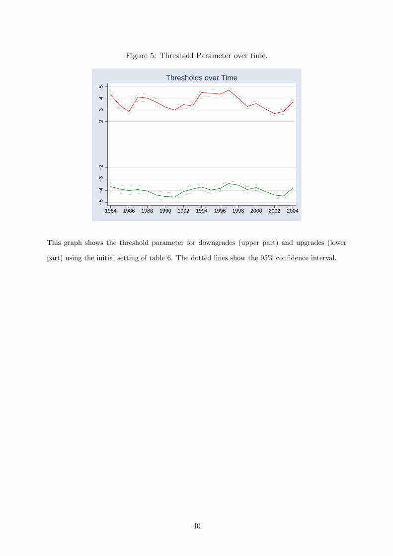
Figure 5: Threshold Parameter over time.

−5

−4

−3

−2

23

45

1984 1986 1988 1990 1992 1994 1996 1998 2000 2002 2004

Thresholds over Time

This graph shows the threshold parameter for downgrades (upper part) and upgrades (lower

part) using the initial setting of table 6. The dotted lines show the 95% confidence interval.

40

Figure 6: Threshold Parameter for different specifications.−

2.5

−2.

75−

3−

3.5

−4

−5

Not

ches

0 6 12 18 24 30D+x LNEDF

D6 RAT D12 RAT D18 RAT D24 RAT D30 RAT

54

32.

52.

252

Not

ches

0 6 12 18 24 30D+x LNEDF

D6 RAT D12 RAT D18 RAT D24 RAT D30 RAT

This graphs shows the threshold parameter for upgrades (left side) and downgrades (right side)

for different parameter specifications. On the x-axis the time-horizon for the independent vari-

able ∆y+xLNEDF increases, while each row shows a different specification of the dependent

variable ∆yRAT .

41

Figure 7: Example of HP-Rating for issuer 551.

−2

−1

01

Tre

nd o

f ED

F

68

1012

1416

Rat

ing

/ HP

−R

atin

g

0 100 200 300Months starting at Jan 1980

Moody’s Rating HP Rating HP EDF

This graphs compares the constructed rating (HPRAT ) based on the Hodrick/Prescott trend

of the EDF (HPEDF ) and Moody’s issuer rating (RAT ).

42

Table 3: Results for the simulation of an ideal through-the-cycle rating.

Panel (A) - One-Year Changes Panel (B) - Two-Year Changes

Full Invest. Grade Spec. Grade Full Invest. Grade Spec. Grade

Dependent Variable ∆12HPRAT ∆24HPRAT

Upgrade Specification

∆12/24LNEDF 1.301 1.276 1.359 1.734 1.718 1.758

(82.3) (66.4) (46.5) (98.1) (81.6) (52.0)

α1 -0.782 -0.651 -1.040 -0.671 -0.522 -0.963

(38.9) (29.7) (25.3) (28.8) (20.3) (20.1)

γ1 0.000 0.000 0.000 0.000 0.000 0.000

(0.0) (0.0) (0.0) (0.0) (0.0) (0.0)

Downgrade Specification

∆12/24LNEDF 1.296 1.377 1.203 1.639 1.754 1.499

(89.1) (71.0) (52.8) (114.9) (92.8) (63.4)

α1 0.834 0.909 0.729 0.596 0.667 0.498

(40.5) (35.0) (21.0) (27.0) (23.9) (12.9)

γ1 0.000 0.000 0.000 0.000 0.000 0.000

(0.0) (0.0) (0.0) (0.0) (0.0) (0.0)

Wald 6,775 4,411 2,163 9,633 6,659 2,707

Log-Likelihood -71,370 -44,181 -25,106 -66,391 -42,001 -20,722

Number of Observations

Total 51,772 32,167 19,605 45,579 29,211 16,368

Upgrade (L) 4,181 2,467 1,714 6,463 4,144 2,319

Frictional (F) 40,068 26,175 13,893 27,525 19,275 8,250

Downgrade (U) 7,523 3,525 3,998 11,591 5,792 5,799

The table presents the results for the regression using a simulated rating based on the Ho-drick/Prescott filter of the EDF. This estimates the bias of the friction model due to the effectof through-the-cycle rating and the method of bucketing. t-statistics are given in parenthesisand calculated using a generalised Hubert-White sandwich estimator for standard errors (seesection 2).

43

Table 4: Results for the initial model including interaction terms and variable threshold

specification.

Panel (A) - One-Year Changes Panel (B) - Two-Year Changes

Full Invest. Grade Spec. Grade Full Invest. Grade Spec. Grade

Dependent Variable ∆12RAT ∆24RAT

Upgrade Specification

∆12/24LNEDF 0.352 0.196 0.510 0.315 0.223 0.471

(9.9) (3.8) (8.5) (11.2) (5.6) (10.0)

· PDRAT-EDF 0.042 -0.193 0.011 0.044 -0.086 0.007

(3.5) (0.7) (0.9) (4.9) (0.5) (0.8)

· VOLAEDF -0.012 -0.029 0.008 0.022 -0.004 0.045

(1.7) (3.5) (0.7) (2.3) (0.5) (3.1)

· BMEDIAN-EDF -0.053 0.189 -0.027 -0.063 0.068 -0.025

(3.4) (0.7) (1.5) (4.6) (0.4) (1.6)

Mean Slope 0.390 0.34 0.460 0.387 0.320 0.491

(2.7) (6.3) (2.2) (1.8) (3.2) (1.7)

Upgrade Threshold

VOLAEDF 0.036 0.031 0.013 0.019 0.006 -0.005

(2.4) (1.2) (0.8) (0.9) (0.2) (0.2)

PDRAT-EDF -0.072 -1.825 -0.069 -0.136 -2.276 -0.134

(4.1) (6.6) (4.3) (5.1) (7.4) (5.1)

BMEDIAN-EDF 0.094 1.907 0.085 0.097 2.320 0.089

(4.6) (6.8) (4.3) (3.7) (7.5) (3.3)

INVEST -0.323 -0.289

(4.3) (3.2)

RECESSION -0.375 -0.574 -0.328 -0.253 -0.234 -0.679

(3.5) (4.0) (2.1) (2.9) (2.4) (4.6)

Cons. -3.666 -4.073 -3.427 -2.588 -3.035 -2.215

(36.0) (39.0) (28.1) (26.0) (31.1) (18.7)

Mean -3.933 -3.894 -3.621 -2.873 -2.788 -2.569

(13.7) (12.8) (12.0) (7.5) (9.6) (4.3)

Downgrade Specification

∆12/24LNEDF 0.571 0.297 0.678 0.519 0.278 0.663

(17.4) (6.2) (14.1) (18.8) (7.4) (16.3)

· PDRAT-EDF 0.036 -0.085 0.011 0.022 0.107 -0.004

(6.0) (0.3) (2.1) (5.3) (0.6) (0.9)

· VOLAEDF -0.004 -0.009 0.006 0.018 0.001 0.025

(0.7) (1.6) (0.6) (1.9) (0.1) (2.4)

· BMEDIAN-EDF -0.070 0.095 -0.036 -0.054 -0.117 -0.017

(7.7) (0.4) (3.6) (7.5) (0.6) (2.2)

Mean Slope 0.621 0.573 0.696 0.572 0.529 0.639

(4.0) (11.8) (3.1) (3.4) (5.8) (2.8)

Downgrade Threshold

VOLAEDF -0.065 -0.069 -0.106 -0.113 -0.143 -0.161

(5.2) (3.1) (8.0) (5.8) (4.1) (8.4)

PDRAT-EDF -0.097 0.777 -0.128 -0.101 0.357 -0.136

(11.3) (2.9) (14.1) (10.6) (1.2) (13.2)

BMEDIAN-EDF 0.110 -0.594 0.129 0.037 -0.237 0.068

(8.0) (2.1) (8.6) (2.2) (0.8) (4.1)

INVEST 0.807 0.967

(11.9) (11.9)

RECESSION -0.394 -0.327 -0.324 -0.237 0.046 -0.720

(4.5) (3.3) (2.4) (3.5) (0.6) (7.6)

Cons. 3.079 3.450 3.535 1.658 2.221 2.246

(43.6) (43.8) (42.0) (22.4) (28.7) (27.8)

Mean 3.397 3.280 3.014 2.077 2.107 1.666

(4.6) (7.1) (3.5) (2.1) (2.6) (4.7)

Wald 136.07 32.10 116.48 202.68 55.19 181.03

Log-Likelihood -48,263 -23,595 -18,734 -61,823 -32,031 -20,788

The table presents the results for the regression of one-year (panel (A)) and two-year (panel (B))rating changes with the respective changes of the EDF. The specification of the latent creditprocess includes interaction terms with the EDF changes. The specification of the thresholds isvariable. The rows ’Mean’ of the threshold specification give the mean thresholds. t-statisticsare given in parenthesis and calculated using a generalised Hubert-White sandwich estimatorfor standard errors (see section 2).

44

Figure 8: Example of Ratings predicted by the friction model.

−3

−2

−1

01

2ln

edf

56

810

1214

15R

atin

g N

otch

es

0 100 200 300Months starting at Jan 1980

Pred. RAT Moody’s RAT LNEDF

−3

−2

−1

01

2ln

edf

56

810

1214

15R

atin

g N

otch

es

0 100 200 300Months starting at Jan 1980

Pred. RAT Moody’s RAT LNEDF

These graphs compare the Moody’s rating with the models prediction without imposing stick-

iness (left side) and with sticky ratings (right side) for the parameter specification of table 6,

panel (B).

45

Table 5: Results of the fully specified model using outlook adjusted ratings.

Panel (A) - One-Year Changes Panel (B) - Two-Year Changes

Full Invest. Grade Spec. Grade Full Invest. Grade Spec. Grade

Dependent Variable ∆12OUTLKRAT ∆24OUTLKRAT

Upgrade Specification

∆12/24LNEDF 0.395 0.336 0.473 0.350 0.273 0.475

(11.1) (6.2) (8.0) (10.7) (5.9) (8.5)

· PDRAT-EDF 0.030 0.630 0.017 0.031 0.484 0.017

(3.5) (2.0) (2.0) (3.9) (2.1) (2.0)

· VOLAEDF 0.031 -0.001 0.045 0.067 0.013 0.071

(2.8) (0.1) (3.1) (5.0) (0.6) (4.5)

· BMEDIAN-EDF -0.054 -0.668 -0.034 -0.059 -0.557 -0.039

(4.5) (2.1) (2.6) (4.7) (2.4) (2.7)

Upgrade Thresholds

VOLAEDF -0.001 0.084 -0.031 0.008 0.104 -0.044

(0.1) (2.0) (1.6) (0.3) (1.9) (1.5)

PDRAT-EDF -0.042 0.616 -0.043 -0.106 -0.174 -0.115

(4.2) (2.0) (4.3) (6.0) (0.5) (6.1)

BMEDIAN-EDF 0.056 -0.569 0.051 0.077 0.194 0.076

(3.7) (1.8) (3.3) (3.4) (0.5) (3.2)

INVEST -0.384 -0.291

(5.7) (3.2)

RECESSION -0.208 -0.032 -0.318 0.052 0.085 -0.266

(2.1) (0.2) (2.1) (0.5) (0.7) (1.7)

Cons. -2.054 -2.440 -1.916 -1.617 -1.922 -1.334

(27.5) (30.2) (21.9) (16.6) (21.4) (11.2)

Mean -2.353 -2.498 -2.129 -1.893 -1.880 -1.746

(12.1) (10.2) (7.3) (5.1) (6.7) (2.6)

Downgrade Specification

∆12/24LNEDF 0.556 0.361 0.604 0.525 0.317 0.642

(14.4) (6.2) (10.8) (14.8) (6.3) (12.3)

· PDRAT-EDF 0.026 -0.038 0.014 0.016 0.064 0.002

(4.6) (0.1) (2.6) (3.4) (0.3) (0.6)

· VOLAEDF 0.007 -0.007 0.015 0.051 0.089 0.036

(0.7) (0.2) (1.3) (3.8) (1.7) (2.9)

· BMEDIAN-EDF -0.057 0.026 -0.031 -0.044 -0.085 -0.020

(5.8) (0.1) (2.9) (5.6) (0.4) (2.3)

Downgrade Thresholds

VOLAEDF -0.025 0.099 -0.076 -0.035 0.139 -0.115

(1.7) (1.8) (5.0) (1.4) (1.9) (4.7)

PDRAT-EDF -0.064 -0.173 -0.075 -0.078 -0.645 -0.093

(7.5) (0.5) (9.0) (7.5) (1.7) (9.0)

BMEDIAN-EDF 0.109 0.426 0.106 0.039 0.795 0.047

(7.2) (1.3) (6.9) (2.1) (2.1)

INVEST 0.735 1.109

(9.9) (11.1)

RECESSION 0.071 -0.013 0.295 0.204 0.381 -0.269

(0.7) (0.1) (1.8) (2.2) (3.3) (2.1)

Cons. 1.854 2.270 2.205 0.662 1.313 1.263

(26.1) (30.0) (25.7) (7.7) (15.9) (13.3)

Mean 2.166 2.251 1.827 1.223 1.400 0.807

(3.8) (6.2) (3.1) (1.6) (3.4) (1.1)

Wald 244.18 45.25 186.92 359.91 104.01 320.23

Log-Likelihood -29,667 -14,863 -12,408 -69,416 -37,702 -23,343

The table presents the results for the regression of one-year (panel (A)) and two-year (panel(B)) rating changes with addition of outlook and watchlist information the respective changesof the EDF. The specification of the latent credit process includes interaction terms with theEDF changes. The specification of the thresholds is variable. The rows ’Mean’ of the thresholdspecification give the mean thresholds. t-statistics are given in parenthesis and calculated usinga generalised Hubert-White sandwich estimator for standard errors (see section 2).

46

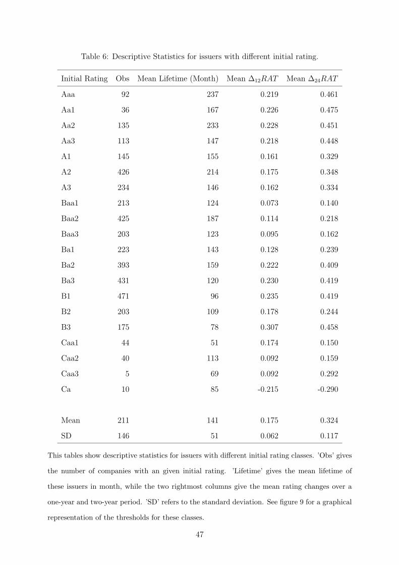
Table 6: Descriptive Statistics for issuers with different initial rating.

Initial Rating Obs Mean Lifetime (Month) Mean ∆12RAT Mean ∆24RAT

Aaa 92 237 0.219 0.461

Aa1 36 167 0.226 0.475

Aa2 135 233 0.228 0.451

Aa3 113 147 0.218 0.448

A1 145 155 0.161 0.329

A2 426 214 0.175 0.348

A3 234 146 0.162 0.334

Baa1 213 124 0.073 0.140

Baa2 425 187 0.114 0.218

Baa3 203 123 0.095 0.162

Ba1 223 143 0.128 0.239

Ba2 393 159 0.222 0.409

Ba3 431 120 0.230 0.419

B1 471 96 0.235 0.419

B2 203 109 0.178 0.244

B3 175 78 0.307 0.458

Caa1 44 51 0.174 0.150

Caa2 40 113 0.092 0.159

Caa3 5 69 0.092 0.292

Ca 10 85 -0.215 -0.290

Mean 211 141 0.175 0.324

SD 146 51 0.062 0.117

This tables show descriptive statistics for issuers with different initial rating classes. ’Obs’ gives

the number of companies with an given initial rating. ’Lifetime’ gives the mean lifetime of

these issuers in month, while the two rightmost columns give the mean rating changes over a

one-year and two-year period. ’SD’ refers to the standard deviation. See figure 9 for a graphical

representation of the thresholds for these classes.

47

Figure 9: Thresholds for different initial ratings.−

5−

4−

3−

22

34

50

1 2 3 4 5 6 7 8 9 10 11 12 13 14 15 16 17 18Initial Rating

Upgrade Threshold Downgrade Threshold

−4

−3

−2

−1

12

34

0

1 2 3 4 5 6 7 8 9 10 11 12 13 14 15 16 17 18Initial Rating

Upgrade Threshold Downgrade Threshold

These graphs shows the evolution of thresholds for issuers with a specific initial rating. The

left graph shows the effect for the one-year model, while the right graph illustrates the two-year

model.

48

Table 7: Overview of thresholds for different specifications.

Threshold

Changes over Dependent Upgrade Downgrade

One-year Moody’s Rating -3.947 3.627

HP Rating (Bias) -0.782 0.834

Outlook/Watchlist adj. Rating -2.385 2.306

Two-years Moody’s Rating -2.886 2.261

HP Rating (Bias) -0.671 0.596

Outlook/Watchlist adj. Rating -1.914 1.338

This table gives an overview of the threshold levels obtained by different specifications of the

dependent variable.

49

Table 8: Idealized Probability of Default.

years

Moody’s Rating 1 2 3 4 5 6 7 8 9 10

Aaa 0.0001% 0.0002% 0.0007% 0.0018% 0.0029% 0.0040% 0.0052% 0.0066% 0.0082% 0.0100%

Aa1 0.0006% 0.0030% 0.0100% 0.0210% 0.0310% 0.0420% 0.0540% 0.0670% 0.0820% 0.1000%

Aa2 0.0014% 0.0080% 0.0260% 0.0470% 0.0680% 0.0890% 0.1110% 0.1350% 0.1640% 0.2000%

Aa3 0.0030% 0.0190% 0.0590% 0.1010% 0.1420% 0.1830% 0.2270% 0.2720% 0.3270% 0.4000%

A1 0.0058% 0.0370% 0.1170% 0.1890% 0.2610% 0.3300% 0.4060% 0.4800% 0.5730% 0.7000%

A2 0.0109% 0.0700% 0.2220% 0.3450% 0.4670% 0.5830% 0.7100% 0.8290% 0.9820% 1.2000%

A3 0.0389% 0.1500% 0.3600% 0.5400% 0.7300% 0.9100% 1.1100% 1.3000% 1.5200% 1.8000%

Baa1 0.0900% 0.2800% 0.5600% 0.8300% 1.1000% 1.3700% 1.6700% 1.9700% 2.2700% 2.6000%

Baa2 0.1700% 0.4700% 0.8300% 1.2000% 1.5800% 1.9700% 2.4100% 2.8500% 3.2400% 3.6000%

Baa3 0.4200% 1.0500% 1.7100% 2.3800% 3.0500% 3.7000% 4.3300% 4.9700% 5.5700% 6.1000%

Ba1 0.8700% 2.0200% 3.1300% 4.2000% 5.2800% 6.2500% 7.0600% 7.8900% 8.6900% 9.4000%

Ba2 1.5600% 3.4700% 5.1800% 6.8000% 8.4100% 9.7700% 10.7000% 11.6600% 12.6500% 13.5000%

Ba3 2.8100% 5.5100% 7.8700% 9.7900% 11.8600% 13.4900% 14.6200% 15.7100% 16.7100% 17.6600%

B1 4.6800% 8.3800% 11.5800% 13.8500% 16.1200% 17.8900% 19.1300% 20.2300% 21.2400% 22.2000%

B2 7.1600% 11.6700% 15.5500% 18.1300% 20.7100% 22.6500% 24.0100% 25.1500% 26.2200% 27.2000%

B3 11.6200% 16.6100% 21.0300% 24.0400% 27.0500% 29.2000% 31.0000% 32.5800% 33.7800% 34.9000%

Caa1 17.3816% 23.2341% 28.6386% 32.4788% 36.3137% 38.9667% 41.3854% 43.6570% 45.6718% 47.7000%

Caa2 26.0000% 32.5000% 39.0000% 43.8800% 48.7500% 52.0000% 55.2500% 58.5000% 61.7500% 65.0000%

Caa3 50.9902% 57.0088% 62.4500% 66.2420% 69.8212% 72.1110% 74.3303% 76.4853% 78.5812% 80.7000%

This graph is reproduced from Yoshizawa (July 29, 2003) and shows the idealized probability of default

in each rating category over different time-horizons.

50