three essays on risk attitudes and the theory of …

THREE ESSAYS ON RISK ATTITUDES AND THE THEORY OF CONTESTS

by

ZHE YANG

PAAN JINDAPON, COMMITTEE CHAIRGREGORY GIVENSPAUL PECORINOMICHAEL PRICERUDY SANTORE

GEORGE ZANJANI

A DISSERTATION

Submitted in partial fulfillment of the requirementsfor the degree of Doctor of Philosophy

in the Department of Economics, Finance, and Legal Studiesin the Graduate School of

The University of Alabama

TUSCALOOSA, ALABAMA

2019

Copyright Zhe Yang 2019ALL RIGHTS RESERVED

ABSTRACT

In the first essay, we prove existence and uniqueness of equilibrium in rent-seeking

contests in which players are heterogeneous in both risk preferences and production

technology. Given identical linear production technology, if the number of risk-loving players

is large enough, the aggregate investment in equilibrium will exceed the rent and all

risk-neutral and risk-averse players will exit the contest. In simultaneous and sequential

contests with two players, we can identify the favorite and underdog based on both players’

preference parameters. Our theoretical results suggest that subjects in some recent contest

experiments behaved as if they were risk-loving.

In the second essay, we prove existence and uniqueness of equilibrium in a game where

heterogeneous risk-averse players contribute to a public good via lottery purchases.

Contrasting models with risk neutrality, we show that an equilibrium with a strictly positive

amount of the public good may not exist without a sufficient number of less risk-averse

participants. We show that more risk-averse players purchase less lotteries and are more likely

to free ride in equilibrium. As a result, it is possible for free riders to place a larger value on

the public good than those who contribute. We also show that there exists an upper bound

for the amount of the public good provided in equilibrium even though the number of players

approaches infinity. Furthermore, we derive a lottery prize that maximizes the equilibrium

amount of the public good and find that such a prize always results in over-provision of the

public good.

In the third essay, we examine the formation of class action lawsuits with plaintiffs

who have heterogeneous degrees of risk aversion. In this model, each plaintiff can either

choose to join the class action or sue the defendant individually. We find that the defendant

prefers settling the case regardless of class status. Less risk-averse plaintiffs can receive higher

settlement offers than more risk-averse plaintiffs and thus have incentives to opt out. We find

ii

that the main role of a self-interested counsel who initiates the class action is to increase the

loss that the defendant incurs. Moreover, class action with a self-interested counsel may not

be able to form if there are enough less risk-averse plaintiffs in an incomplete information

structure. However, the class action can benefit all plaintiffs if they are risk-averse enough

and have no incentive to sue the defendant individually when the class action is available.

iii

DEDICATION

To my parents. Thank you for your support in allowing me to pursue my dream.

Words fail to express my gratitude.

iv

ACKNOWLEDGMENTS

I would like to thank Dr. Paan Jindapon for being my mentor since the first day I met

him. It would be an impossible work to complete this dissertation without his guidance and

support. He never hesitates to share his knowledge and ideas with me. I have learnt not only

how to do research but also how to be a good researcher and a teacher by working with him.

His academic vision and passion for economics will always be the standard in my future career.

My gratitude also goes out to Dr. Paul Pecorino. He has been an invaluable asset in

writing the last chapter of my dissertation. I would also like to thank the other members of

my committee, Dr. Gregory Givens, Dr. Michael Price, Dr. Rudy Santore, and Dr. George

Zanjani for their insightful comments.

A special posthumous thank you to Dr. Harris Schlesinger for advising me for the first

several years in the PhD program and inspiring my passion for research.

Finally, I would like to express my gratitude to the entire faculty and staff of the

Department of Economics, Finance and Legal Studies for making my time in this program

worthwhile. I would like to extend my appreciation to my classmates, Dr. Chi-Yang Chu and

Michael Solomon. Their suggestions for my presentations for my dissertation are always

helpful.

v

CONTENTS

ABSTRACT . . . . . . . . . . . . . . . . . . . . . . . . . . . . . . . . . . . . . . . . . . ii

DEDICATION . . . . . . . . . . . . . . . . . . . . . . . . . . . . . . . . . . . . . . . . . iv

ACKNOWLEDGMENTS . . . . . . . . . . . . . . . . . . . . . . . . . . . . . . . . . . . v

LIST OF TABLES . . . . . . . . . . . . . . . . . . . . . . . . . . . . . . . . . . . . . . . viii

LIST OF FIGURES . . . . . . . . . . . . . . . . . . . . . . . . . . . . . . . . . . . . . . ix

CHAPTER 1. RISK ATTITUDES AND HETEROGENEITY IN SIMULTANEOUS

AND SEQUENTIAL CONTESTS . . . . . . . . . . . . . . . . . . . . . . . . . 1

1. Introduction . . . . . . . . . . . . . . . . . . . . . . . . . . . . . . . . . . . . . . . . 1

2. Existence and Uniqueness of Equilibrium . . . . . . . . . . . . . . . . . . . . . . . . 4

3. Generalized CARA Players . . . . . . . . . . . . . . . . . . . . . . . . . . . . . . . . 8

4. Sequential Contests . . . . . . . . . . . . . . . . . . . . . . . . . . . . . . . . . . . . 15

4.1. Subgame-Perfect Equilibrium . . . . . . . . . . . . . . . . . . . . . . . . . . . . . . 16

4.2. Favorites and Underdogs . . . . . . . . . . . . . . . . . . . . . . . . . . . . . . . . 19

5. Conclusion and Discussion . . . . . . . . . . . . . . . . . . . . . . . . . . . . . . . . . 21

CHAPTER 2. FREE RIDERS AND OPTIMAL PRIZE IN PUBLIC GOOD

FUNDING LOTTERY . . . . . . . . . . . . . . . . . . . . . . . . . . . . . . . . . 25

1. Introduction . . . . . . . . . . . . . . . . . . . . . . . . . . . . . . . . . . . . . . . . 25

2. Existence and Uniqueness of Equilibrium . . . . . . . . . . . . . . . . . . . . . . . . 27

3. Comparative Statics . . . . . . . . . . . . . . . . . . . . . . . . . . . . . . . . . . . . 31

4. Optimal Lottery Prize . . . . . . . . . . . . . . . . . . . . . . . . . . . . . . . . . . . 35

5. Conclusion . . . . . . . . . . . . . . . . . . . . . . . . . . . . . . . . . . . . . . . . . 38

CHAPTER 3. RISK AVERSION IN CLASS ACTION SUITS . . . . . . . . 40

vi

1. Introduction . . . . . . . . . . . . . . . . . . . . . . . . . . . . . . . . . . . . . . . . 40

2. The Model . . . . . . . . . . . . . . . . . . . . . . . . . . . . . . . . . . . . . . . . . 43

3. The Formation of a Class with Perfect Information . . . . . . . . . . . . . . . . . . . 49

4. The Formation of a Class with Incomplete Information . . . . . . . . . . . . . . . . . 51

5. Conclusion and Discussion . . . . . . . . . . . . . . . . . . . . . . . . . . . . . . . . . 54

REFERENCES . . . . . . . . . . . . . . . . . . . . . . . . . . . . . . . . . . . . . . . . . 56

APPENDIX A . . . . . . . . . . . . . . . . . . . . . . . . . . . . . . . . . . . . . . . . . 61

APPENDIX B . . . . . . . . . . . . . . . . . . . . . . . . . . . . . . . . . . . . . . . . . 68

APPENDIX C . . . . . . . . . . . . . . . . . . . . . . . . . . . . . . . . . . . . . . . . . 75

vii

LIST OF TABLES

1 Theoretical predictions and actual investments in simultaneous contests . . . . . . . . 23

viii

LIST OF FIGURES

1 Share function and equilibria in Examples 1, 2, and 3 . . . . . . . . . . . . . . . . . . 10

2 Aggregate investment in standard Tullock contest with n homogeneous players . . . . 14

3 Subgame-perfect equilibria in which (a) player 2 participates and (b) does not participate 18

4 Estimation of θiαi for i = 10 in Session 1 of Fonseca’s experiment . . . . . . . . . . . 24

5 Share functions given ui(wi, G) = −e−(αiwi+βiG) and R = 0.5 . . . . . . . . . . . . . . 32

6 Optimal lottery prize and public good provision given n . . . . . . . . . . . . . . . . 38

ix

CHAPTER 1. RISK ATTITUDES AND HETEROGENEITY IN

SIMULTANEOUS AND SEQUENTIAL CONTESTS

1. Introduction

Tullock (1980) introduces a seminal framework to analyze winner-take-all contests in

which each player competes with one another to win a given prize (also called rent). The

winning probability of each player is determined by his irreversible investment relative to the

total investment by all players participating in the contest. In this paper, we study a class of

rent-seeking contests with heterogeneity in players’ risk preferences and production

technology. To the best of our knowledge, this paper is the first to show that there is a unique

equilibrium in rent-seeking contests where some players are risk-averse and some are

risk-loving. We first assume a class of utility functions that are bivariate, i.e., a player’s utility

is a function of two variables, his final wealth and the prize received from the contest. This

functional form allows us to identify an equilibrium in a contest that awards the winner with

a non-monetary prize. For contests with a cash prize, as a special case, we can write each

player’s utility function as a univariate function which exhibits constant absolute risk aversion

(CARA). Since each function could be concave, linear, or convex, we call this class of utility

functions “generalized CARA.”

In addition to proving existence and uniqueness of equilibrium given heterogeneous

players, we expand the literature of rent-seeking contests in three directions. First, we

theoretically show that, under Expected Utility Theory, rent over-dissipation or

under-dissipation may occur in equilibrium (i.e., total rent-seeking investment by all

participants may or may not exceed the rent) depending on number of players and each

player’s preference parameters. While rent over-dissipation seems to be a more important

issue to economists and policy makers since it implies excess social waste, both rent

1

over-dissipation and under-dissipation are empirically supported in laboratory settings.1

Assuming linear utility functions, Tullock (1980) uses numerical examples to show that rent

may be over-dissipated given a class of convex rent-seeking production functions. However,

Baye et al. (1994 and 1999) argue that pure-strategy equilibrium does not exist in those cases

and thus rent over-dissipation is not possible under risk neutrality.2 Contrasting Tullock’s

theoretical approach in explaining rent over-dissipation, we assume linear technology and let

some players be risk-loving. While Jindapon and Whaley (2015) show that the more

risk-loving players participating in the contest, the more likely rent over-dissipation will occur

in equilibrium, with our generalized CARA functional form, we can be more specific about

the number of risk-loving players that is sufficient or necessary for rent over-dissipation.

Specifically, if the number of risk-loving players is larger than a threshold, which is greater

than 4, then rent over-dissipation will occur in equilibrium. Moreover, in such an equilibrium,

we find that all risk-neutral and risk-averse players will not participate in the contest.

Second, this paper is the first to analyze risk attitudes in sequential rent-seeking

games. Since the seminal analysis of preemptive investment by Dixit (1987), most theoretical

development in the literature has been on rent-seeking technology (i.e., contest success

functions) and asymmetry in reward and information3 while players’ risk attitudes have been

ignored. By allowing for nonlinear utility functions, we can derive results contradicting Dixit’s

(1987) well-known prediction that there is no incentive to move first in a standard Tullock

contest. Specifically, we find that even when both players have the same preferences and

rent-seeking technology, the first mover will be the favorite to win if both players are

risk-averse. On the other hand, if both players are risk-loving, the first mover will become the

underdog. In a sequential contest with heterogeneous players, we find that if the first mover is

less/more downside-risk-averse and the second mover is risk-averse/loving, then the first

mover will be the favorite/underdog in the contest, respectively.

1See Houser and Stratmann (2012) and Sheremeta (2013) for thorough reviews of experimental findings.2See also Cornes and Hartley (2005).3For example, Baik and Shogren (1992), Baye and Shin (1999), Morgan (2003), and Morgan and Vardy (2007).

2

Finally, this paper provides important applications in empirical research. Even though

risk aversion may seem to be a standard presumption of human behavior, researchers found

that some decision makers especially in the laboratory or the field behaved as if they were

risk-loving.4 Focusing on pay-to-bid auctions, Platt et al. (2013) suggest that pay-to-bid

auction is a mild form of gambling and allowing for risk lovingness has the biggest impact in

explaining bidding behavior. To some experimental subjects, investing in a rent-seeking

contest may be a form of gambling, so allowing for risk lovingness should help rationalize

rent-seeking behavior as well. While recent developments in the literature suggest that

different equilibrium concepts (Gneezy and Smorodinsky, 2006, and Lim et al., 2014) or

psychological factors (Sheremeta, 2013) can explain rent over-dissipation in the laboratory,

our theoretical predictions provide a possible explanation for such a phenomenon under the

canonical expected utility model.

To evaluate our nonlinear utility model in explaining empirical findings, we reexamine

experimental data from simultaneous contests in Sheremeta (2011) and Lim, Matros, and

Turocy (2014). We find that, by allowing subjects to be risk-loving, we can estimate a risk

parameter that yields a theoretical prediction that is much closer to average rent-seeking

behavior in the laboratory than when we assume risk neutrality. We also analyze data from

two-player sequential contests in Fonseca (2009). Focusing on behavior of second movers, we

estimate preference parameters of these subjects based on their responses to first-mover

investment and find that all second-mover subjects are risk-loving.

This paper is organized as follows. In Section 2, we prove existence and uniqueness of

equilibrium in simultaneous contests given a class of bivariate utility functions. We derive

sufficient conditions for rent over-dissipation and under-dissipation in equilibrium given

generalized CARA players in Section 3. We prove existence and uniqueness of equilibrium in

sequential contests and derive sufficient conditions for first- and second-mover advantages in

Section 4. We conclude and discuss experimental evidence in Section 5.

4See Isaac and James (2000), Berg et al. (2005), Eckel et al. (2009), Bellemare and Shearer (2010), and Platt etal. (2013). Interestingly, Isaac and James (2000) and Berg et al. (2005) also find inconsistency in risk attitudesacross institutions.

3

2. Existence and Uniqueness of Equilibrium

Consider an n-player contest for a fixed prize R with n ≥ 2 and R > 0. For i = 1, ..., n,

player i has an initial wealth Ii and invests xi in the contest. The probability that player i

wins the prize depends on xi and all other players’ investment as specified in the following

assumption.

Assumption 1. Player i’s probability of winning the prize from investing xi in the contest is

given by

pi =fi(xi)∑nj=1 fj(xj)

(1)

where fi(xi) is player i’s production function. We assume that fi is a twice differentiable

function with fi(0) = 0, f ′i(xi) > 0, and f ′′i (xi) ≤ 0 for all xi ≥ 0.

Player i’s production or output generated by investing xi is fi(xi) which is a strictly

increasing function with non-increasing marginal productivity. In a standard Tullock contest,

fi(xi) = xi for all i. When player i invests nothing in the contest, his output is zero and so is

the probability of winning the prize.5 Player i’s probability of winning is strictly increasing in

his own investment and decreasing in investment by other players.

Each player’s utility depends on his final wealth and whether he wins the contest.

Specifically, we assume that player i’s utility is a function of two variables, his final wealth

wi = Ii − xi and the received prize ri ∈ {0, R}.

Assumption 2. Player i’s utility is derived from

ui(wi, ri) =

θie

θi[Ai(wi)+Bi(ri)] if θi 6= 0

wi + Ci(ri) if θi = 0

(2)

where

(i) θi ∈ {−1, 0, 1},

5If xi = 0 for all i, the function in (1) is undefined so we impose that pi = 0 for all i.

4

(ii) Ai is a twice differentiable function with Ai(wi) ≥ 0, A′i(wi) > 0, and

0 ≥ A′′i (wi) ≥ −[A′i(wi)]2 for all wi ≥ 0, and

(iii) Bi and Ci are functions of ri with Bi(R) > Bi(0) = 0 and Ci(R) > Ci(0) = 0.

The utility function in Assumption 2 is strictly increasing in wi. The sign of

∂2ui(wi, ri)/∂w2i is the same as the sign of θi[A

′i(wi)]

2 + A′′i (wi) so the last condition in part

(ii) of Assumption 2 implies that the utility function is concave or convex in wi if θi = −1 or

1, respectively. As a result, we can use our model to analyze a contest when risk-averse,

risk-neutral, and risk-loving players are all present together. Moreover, we are able to analyze

heterogeneity in risk preferences. Since Ai and Aj are allowed to be different functions,

players i and j may have different degrees of risk aversion (or risk lovingness).6

Another important feature of our utility function is its domain which consists of wealth

and prize as two separate variables. Since the received prize does not need to be directly

added to the winner’s final wealth, this functional form allows us to analyze a contest that

rewards the winner with a non-cash prize. For example, we may assume that θi = −1,

Ai(wi) = ln(wi + 1), and Bi(ri) = ri, so that player i’s utility can be written as

ui(wi, ri) =

− 1wi+1

if he does not win the contest, i.e., ri = 0

− e−R

wi+1if he wins the contest, i.e., ri = R

(3)

which is strictly concave in wi.

For cash-prize contests which are much more common in the literature, we assume that

Ai and Bi are identical linear functions so that player i’s utility is a function of the sum of wi

and ri. For example, if Ai(wi) = αiwi and Bi(ri) = αiri with αi > 0, player i’s utility can be

written as ui(wi, ri) = θieθiαi(wi+ri) for θi 6= 0 which is a CARA utility function. This utility

function is strictly concave if θi = −1 and strictly convex if θi = 1. Cornes and Hartley (2003)

prove that an equilibrium uniquely exists given players with concave CARA utility functions.

6It follows from (3) that when θi 6= 0, player i’s Arrow-Pratt absolute measure of risk aversion given wi is

γi(wi) = −[A′′i (wi)A′i(wi)

+ θiA′i(wi)

]. Note that γi(wi) does not depend on Bi(r). If Ai(wi) = ln(wi + 1), then

γi(wi) = 1−θiwi+1 and hence ui(wi, ri) exhibits DARA given θi = −1. If Ai(wi) = αiwi where αi > 0, then

γi(wi) = −θiαi and ui(wi, ri) is a CARA function.

5

In this paper, we prove existence and uniqueness of equilibrium not only for convex CARA

functions, but also for any other functions satisfying Assumption 2.

Following Szidarovszky and Okuguchi (1997), we define yi = fi(xi) as player i’s output

level and let Y−i =∑

j 6=i yj be the sum of all other players’ output. This approach is useful for

identifying equilibrium in aggregative games, especially rent-seeking contests where player i’s

strategy depends on aggregate rent-seeking production by all other players.7 Since fi is

bijective, we can define gi = f−1i as player i’s investment cost of output yi. According to

Assumption 1, we know that gi(0) = 0, g′i(yi) ≥ 0, and g′′i (yi) ≥ 0 for all yi ≥ 0. Furthermore,

we can rewrite the probability of winning in (1) as

pi =yi

yi + Y−i(4)

and say that player i chooses an optimal output yi, rather than an investment xi, to maximize

his expected utility. Player i’s expected utility as a function of yi conditional on Y−i can be

written as

Ui(yi|Y−i) =yi

yi + Y−iui(Ii − gi(yi), R) +

Y−iyi + Y−i

ui(Ii − gi(yi), 0). (5)

Note that Ui(0|0) is undefined yet it is not relevant since player i’s optimal choice of yi to

maximize (5) is strictly positive given Y−i = 0. In this paper, we use Cornes and Hartley’s

(2003, 2005, 2012) concept of share functions to derive an equilibrium. Given his optimal

production denoted by y∗i , we derive player i’s share, i.e., the probability of winning

corresponding to his best response as a function of total production, from si(Y ) = y∗i /Y

where Y = y∗i + Y−i. We find that if Assumptions 1 and 2 hold, we can derive each player’s

participation threshold denoted by κi. Specifically, if Y−i ≥ κi, player i will not participate in

the contest and hence si(Y ) = 0 for all Y ≥ κi.

7Under the assumption that fi is concave, Szidarovszky and Okuguchi (1997) show that an equilibrium uniquelyexists given risk-neutral players. Cornes and Hartley (2003) and Jindapon and Whaley (2015) use Szidarovszkyand Okuguchi’s approach to derive the existence and uniqueness result by assuming concave CARA utilityfunctions and convex utility functions, respectively. Jensen (2016) uses this approach to show that concaveproduction is not necessary for existence and uniqueness of equilibrium when players’ utility functions areseparable in their final wealth and rent-seeking effort, i.e., effort is non-monetary.

6

Lemma 1. Suppose that Assumptions 1 and 2 hold. There exists a participation threshold for

player i given by

κi =

eθiBi(R)−1θiA′i(Ii)g

′i(0)

if θi 6= 0

Ci(R)g′i(0)

if θi = 0.

(6)

Proof. See Appendix A. �

Player i will not participate in the contest if the total production Y is greater than his

threshold κi derived in Lemma 1. If f ′i(0) =∞, then g′i(0) = 0 and (6) suggests that κi =∞.

As a result, this player will always participate even when Y is very large. The following

Lemma shows how player i derives his optimal probability of winning given aggregate

production by all players in the contest.

Lemma 2. Suppose that Assumptions 1 and 2 hold. There exists a unique share function

si(Y ) for player i such that si(Y ) = 0 for Y ≥ κi. For Y ∈ (0, κi), si(Y ) is derived from

g′i(si(Y )Y )Y =

(1−si(Y ))(eθiBi(R)−1)

(si(Y )(eθiBi(R)−1)+1)θiA′i(Ii−gi(si(Y )Y ))if θi 6= 0

(1− si(Y ))Ci(R) if θi = 0.

(7)

Player i’s share function has the following properties:

(1) si(Y ) is continuous in Y for all Y > 0.

(2) si(Y ) is strictly decreasing in Y given Y ∈ (0, κi).

(3) limY→0 si(Y ) = 1 and limY→κi si(Y ) = 0.


Given Y ∈ (0, κi), we cannot explicitly solve for the share function si(Y ) defined in

(29) without a specific functional form of gi. Nonetheless, the three important properties of

si(Y ) derived in Lemma 2 can help us prove existence and uniqueness of equilibrium.8

Property 3 implies that∑n

i=1 si(Y )→ n as Y → 0 and∑n

i=1 si(Y )→ 0 as

8These three desired properties of share functions are jointly sufficient for existence and uniqueness of equilibrium(in Proposition 1) and similar to those derived in Cornes and Hartley (2003) and Jindapon and Whaley (2015).

7

Y → max{κ1, ..., κn}. Since each player’s share function is continuous and strictly decreasing

in Y ∈ (0, κi) (by Properties 1 and 2), the sum of all shares is continuous and strictly

decreasing in Y ∈ (0,max{κ1, ..., κn}). Thus, there exists a unique value of Y such that∑ni=1 si(Y ) = 1, i.e., the aggregate production that constitutes an equilibrium. We call this

value Y e and it follows that each player’s output corresponding to the aggregate output in

equilibrium is yei = si(Ye)Y e. We can derive each player’s equilibrium rent-seeking investment

from xei = gi(yei ) and call the total investment in equilibrium Xe which is equal to

∑ni=1 x

ei .

We formally state our main result as follows.

Proposition 1. Consider a simultaneous contest with n heterogeneous players. If

Assumptions 1 and 2 hold, there exists a unique Nash equilibrium for the contest. In such an

equilibrium, player i invests xei = gi(si(Ye)Y e) where Y e satisfies

∑ni=1 si(Y

e) = 1.

Proof. See the above argument. �

3. Generalized CARA Players

The existence and uniqueness result found in the previous section holds for a very

general class of utility functions. According to Assumption 2, each player’s utility is a

function of two separate variables, his final wealth and the received prize, so that the contest

prize is allowed to be non-monetary. Like most of the literature, we analyze in this section

contests where prize is paid in cash. Specifically, we assume that Ai(wi) = αiwi, Bi(ri) = αiri,

and Ci(ri) = ri so that the received prize can be directly added to the contest winner’s

wealth. Given θi ∈ {−1, 0, 1} and αi ∈ (0,∞), we use θiαi, which is equal to the negative

value of player i’s Arrow-Pratt measure of absolute risk aversion, to represent his type. If we

compare two player types and find θiαi < θjαj, then we can say that player i is more

risk-averse than player j. Moreover, since the Arrow-Pratt measure of absolute risk aversion

for player i is constant given any level of wealth, we say that each player’s utility function has

a generalized CARA form.

8

Definition 1. Player i’s utility function has the generalized CARA form if, for θi ∈ {−1, 0, 1}

and αi ∈ (0,∞), ui(wi, ri) can be written as

vi(wi + ri) =

θie

θiαi(wi+ri) if θi 6= 0

wi + ri if θi = 0.

(8)

Since this utility function is a special case of Assumption 2, a contest equilibrium

uniquely exists if each player’s utility function is given by (8) and production function satisfies

Assumption 1. Consider the following example.

Example 1: Let R = 1 and n = 3. Player 1 has θ1 = −1 and α1 = 1. Player 2 has θ2 = 0.

Player 3 has θ3 = 1 and α3 = 2. Let fi(xi) = xi, that is, gi(yi) = yi, for all i. According to (6),

we find that κ1 = 0.632, κ2 = 1, and κ3 = 3.195. Figure 1 (a) illustrates each player’s share

function. The only value of Y that makes the sum of all shares equal to 1, or Y e, is 0.579

indicated by the vertical line in the figure. Each player’s share function implies that the

probabilities of winning the rent for players 1, 2, and 3 (i.e., si(0.579) for i = 1, 2, 3) are 0.200,

0.421, and 0.379, respectively. It follows that ye1 = 0.200× 0.579 = 0.116 and

xe1 = g1(0.115) = 0.115. Similarly, we find xe2 = 0.244 and xe3 = 0.219. �

Cornes and Hartley (2003) show that if all players are assumed to be risk-averse and

have the same production function, there is a monotonic relationship between each player’s

measure of risk aversion and his investment in equilibrium. Specifically, Cornes and Hartley

find that a more-risk-averse player invests less than a less-risk-averse player in equilibrium.

This result however does not hold when some players are risk-loving as allowed in our model.

Unlike contests with only risk-averse players, we cannot say that xei is decreasing in player i’s

absolute measure of risk aversion. In the equilibrium of Example 1, player 2 who is

risk-neutral invests more than player 3 who is risk-loving.

In the next proposition, we derive each player’s conditions for participating in

equilibrium.

9

0 0.2 0.4 0.6 0.8 1 1.2 1.40

0.2

0.4

0.6

0.8

1

Player 1

Player 2

Player 3

Y

si

Y e

(a) Example 1

0 0.2 0.4 0.6 0.8 1 1.2 1.40

0.2

0.4

0.6

0.8

1

Player 1

Player 2

Players 3 - 7

Y

si

Y e

(b) Example 2

0 1 2 3 4 5 60

0.2

0.4

0.6

0.8

1

Player 1

Player 2

Players 3 - 22

Y

si

Y e

(c) Example 3

Figure 1. Share function and equilibria in Examples 1, 2, and 3

Proposition 2. Consider a simultaneous contest in which each player’s utility function has

the generalized CARA form and production function satisfies Assumption 1. There exists a

unique Nash equilibrium in which player i invests xei .

(1) If f ′i(0) =∞, then xei > 0.

(2) Suppose that f ′i(0) <∞ for all i and fi = fj for i, j = 1, ..., n. If θ1α1 ≤ ... ≤ θnαn,

then κ1 ≤ ... ≤ κn. It follows that if there exists player k such that xek = 0, then xei = 0

for i = 1, ..., k − 1.


The first condition is very intuitive. If player i’s marginal productivity when investing

zero is infinitely large, then in equilibrium player i must participate in the contest regardless

10

of his risk attitude or how many other players he is competing with. The second condition

states that if all players have the same production function with a finite marginal productivity

at zero, then we can rank the players’ participation thresholds by types represented by θiαi.

Part 2 of proposition 2 suggests that a player who is more risk-averse will have a smaller

participation threshold. Therefore, if Y e is so large that there is a player choosing not to

participate in equilibrium, all the players who are more-risk-averse will not participate in the

contest either. Consider the following example.


Each of players 3-7 has θi = 1 and αi = 2. Let fi(xi) = xi, that is, gi(yi) = yi, for all i. We

find that the value of Y such that the sum of all shares equals one is 1.122 (see the vertical

line in Figure 1 (b)). Since both κ1 and κ2 are smaller than 1.122, players 1 and 2 do not

participate in the contest. Each of players 3 to 7 invests 0.224 and, therefore, has an equal

chance of winning the rent. The total investment in the contest is 1.120. �

We show in Example 2 that a large number of risk-loving players can drive

more-risk-averse players out of the contest as suggested by part 2 of Proposition 2. Another

important finding from Example 2 is that the sum of all participating players’ investment is

greater than R, i.e., rent over-dissipation occurs in this equilibrium. In the next example, we

show that rent over-dissipation can occur in equilibrium given a strictly concave production

function as well. In this example, f ′i(0) =∞ for all i so all players participate in the contest

as suggested by part 1 of Proposition 2.


Each of players 3-22 has θi = 1 and αi = 2. Let fi(xi) =√xi, that is, gi(yi) = y2

i , for all i. We

find that the value of Y such that the sum of all shares equals one is 4.920 (see the vertical

line in Figure 1 (c)). We find that s1(4.920) = 0.013, s2(4.920) = 0.020, and

s3(4.920) = ... = s22(4.920) = 0.048. It follows that xe1 = 0.004, xe2 = 0.010, and

xe3 = ... = xe22 = 0.056. Thus, the total investment in the contest is 1.134.

11

In the last two examples, risk-loving players’ aggressive strategies cause rent

over-dissipation to take place in equilibrium. Example 3 in particular yields two interesting

results. First, rent over-dissipation occurs despite the fact that each player’s marginal

productivity of rent-seeking investment is strictly decreasing.9 Second, even though rent

over-dissipation is driven by risk-loving players’ strategies, we find that risk-averse and

risk-neutral players still participate in the contest. This result, however, will not hold in a

standard Tullock contest as discussed below.

More intuitive results can be obtained in a standard Tullock contest. We assume

hereafter that all players have the same production function given by fi(xi) = xi so that

Xe = Y e and xei = yei for all i.10 In addition, player i’s participation threshold (6) and share

function (29) can be written as

κi =

eθiαiR−1θiαi

if θi 6= 0

R if θi = 0

(9)

and

si(Y ) =

κi−Y

κi−Y+Y eθiαiRif Y < κi

0 if Y ≥ κi

(10)

respectively.


the generalized CARA form and production function is given by fi(xi) = xi for i = 1, ..., n.

(1) κi T R if and only if θi T 0.

(2) ∂2si(Y )∂Y 2 T 0 if and only if θi T 0.

9While Tullock (1980) provides numerical examples of rent over-dissipation driven by strictly convex productionfunction, there is no equilibrium supporting his calculation. See discussions in Baye, Kovenock, and de Vries(1994, 1999).10In fact, all of the following results also hold for fi(xi) = axi where a > 0 for all i. For contests withhomogeneous linear technology, we let a = 1 as in a standard Tullock contest without loss of generality. Whileit is possible to relax this assumption by assuming that fi(xi) = aixi with ai > 0 and allowing for asymmetrictechnology among players, we leave this extension for future research.

12


Proposition 3 suggests that for a risk-averse/neutral/loving player, his participation

threshold κi is smaller than/equal to/greater than the rent and his share function is

concave/linear/convex for Y ∈ (0, κi), respectively. In Example 1, we calculate each player’s

participation threshold and plot each share function in Figure 1 (a). As we can see in the

example, κi ≤ R for player i whose θi = −1 or 0. In Example 2, both risk-averse and

risk-neutral players, i.e., players 1 and 2, choose xei = 0 in equilibrium because κi ≤ R < Xe

as suggested by part 1 of Proposition 3. Moreover, Xe > R also implies that some players

must be risk-loving because only risk-loving players have si(Y ) > 0 given Y > R. We conclude

these necessary conditions for rent over-dissipation in a standard Tullock contest in the

following corollary.

Corollary 1. Consider a simultaneous contest in which each player’s utility function has the

generalized CARA form and production function is given by fi(xi) = xi for i = 1, ..., n.

Suppose that rent over-dissipation occurs in equilibrium.

(1) All risk-averse and risk-neutral players choose not to participate in the contest.

(2) Some players are risk-loving.

In Example 1, player 3 is the only risk-loving player in the contest. We find that

Xe < R < κ3. If there are many replicas of player 3, it may be possible to have Xe ∈ (R, κ3)

and, therefore, rent over-dissipation in equilibrium. In Example 2, we add four players whose

utility functions are identical to player 3’s and find that Xe > R in equilibrium—see Figure 1

(b). How many risk-loving players would be large enough for rent over-dissipation to occur in

equilibrium? To answer this question, we consider a special case where there are n identical

risk-lovers in the contest.

Given θi = θ and αi = α for all i = 1, ..., n, then κi = κ for all i = 1, ..., n. By letting

si(Y ) = 1n, we find from (10) that in a standard Tullock contest with homogeneous players,

Xe = Y e =(n− 1)κ

n+ θακ. (11)

13

−6 −4 −2 0 2 4 6 8 100

0.5

1

1.5

2

n = 2

n = 4

n = 6

n = 8

Rent over-dissipation

Rent under-dissipation

θα

Xe

Risk-averse Risk-loving

Figure 2. Aggregate investment in standard Tullock contest with nhomogeneous players

We plot Xe on θα given R = 1 in Figure 2. We also divide the graph into four

quadrants based on risk attitudes and whether rent over-dissipation occurs in equilibrium.

The left/right quadrant corresponds to total investment in equilibrium given risk-averse/loving

players and the top/bottom quadrant indicates rent over/under-dissipation, respectively. We

can see that rent over-dissipation occurs only when the players are risk-loving and n is large.

In general, by substituting θ = 1 and κ from (9) into (11), we find that Xe > R if and only if

(n− 1)(eαR − 1)

(n+ eαR − 1)α> R. (12)

Given the above inequality, we can derive the following results.


the generalized CARA form, with θi = θ and αi = α, and production function is given by

fi(xi) = xi for i = 1, ..., n.

(1) Rent over-dissipation occurs in equilibrium if and only if θ = 1 and n > 1 + αReαR

eαR−αR−1.

(2) Rent over-dissipation will never occur in equilibrium if n ≤ 4.


Under the assumption that all players are identical, rent over-dissipation occurs if and

only if the players are risk-loving and the number of players is large enough. We derive the

14

minimum number of players to guarantee rent over-dissipation in part 1 of Proposition 4.

Note that this minimum number of risk-loving players is not monotonic in α. For example,

given R = 1, when α = 0.5, 1, and 4, we need at least 7, 5, and 6 players, respectively, for rent

over-dissipation to take place in equilibrium. In part 2, we find that n > 4 is necessary but

not sufficient for rent over-dissipation.

4. Sequential Contests

In this section, we analyze sequential contests with two generalized CARA players.

Specifically, we let player 1 choose her rent-seeking investment first and allow player 2 to

observe player 1’s investment before choosing his own investment. Our goals are to prove that

a subgame-perfect equilibrium uniquely exists and to show whether there is an advantage for

a player to move first or second. Before we discuss results from the sequential setting, we first

derive an equilibrium given two players in a simultaneous contest as a benchmark.

For i = 1, 2, player i chooses xi given xj, where j 6= i, to maximize

Vi(xi, xj) =

(xi

x1 + x2

)vi(Ii − xi +R) +

(xj

x1 + x2

)vi(Ii − xi) (13)

where vi has the functional form in (8). The following proposition suggests that in a

simultaneous contest with two players, we can identify the favorite and underdog based on

each player’s preference parameters θi and αi.

Proposition 5. Consider a simultaneous two-player contest in which each player’s utility

function has the generalized CARA form and production function is given by fi(xi) = xi for

i = 1, 2. If |θ1α1| S |θ2α2|, then xe1 T xe2.


If the two players move simultaneously, the favorite to win is the one with a smaller

value of |θiαi|. Therefore, when neither of the players is risk-neutral, the favorite is the one

with a smaller αi regardless of the sign of θi. Even though one of the players is risk-loving and

the other is risk-averse, they will invest the same amount in equilibrium whenever α1 = α2.

15

Proposition 5 also implies that the player who is less downside-risk-averse will be the

favorite to win the contest.11 The effect of downside risk aversion on rent-seeking investment

is analogous to that on loss-prevention decision—also known as the self-protection problem

first studied by Ehrlich and Becker (1972). In a loss-prevention problem an agent invests to

reduce the probability of undesired outcome in the loss state, while in a contest a player

invests to increase the probability of winning which is the desired outcome of the game. Thus,

the two problems are equivalent if we ignore strategic interaction in the contest setting. The

role of downside risk attitudes on loss prevention has been analyzed by Eeckhoudt and Gollier

(2005), Jindapon and Neilson (2007) and Crainich and Eeckhoudt (2008); a common finding

is that downside risk aversion has a negative impact on optimal loss-prevention effort. Using

this analogy, Treich (2010) proves that risk aversion decreases rent-seeking investment in a

symmetric contest under the condition of downside risk aversion. Jindapon and Whaley

(2015) complement Treich’s result by showing that risk lovingness increases rent-seeking

investment given downside-risk-loving players.

4.1. Subgame-Perfect Equilibrium. Since the share function approach we adopted in

Sections 2 and 3 is not compatible with sequential-move games, we identify an equilibrium of

a sequential contest by solving the problem backward as conventionally done in a Stackelberg

game. Specifically, we derive player 2’s best-response function and then solve player 1’s

optimization problem given player 2’s best response. For i = 1, 2, player i’s expected utility

given the other player’s investment is given by (13).

In period 2, taking x1 as given, we derive the first-order condition for player 2’s interior

solution by setting Φ2(x1, x2) := ∂V2∂x2

= 0. Given θ2 6= 0, we have

Φ2(x1, x2) =θ2e

θ2α2(I2−x2)

(x1 + x2)2

[x1(eθ2α2R − 1)− θ2α2x2(x1 + x2)(eθ2α2R − 1)− θ2α2(x1 + x2)2

]= 0.

(14)

11Modica and Scarsini (2005) define a measure of downside risk aversion for player i evaluated at w as Di(w) =v′′′i (w)v′i(w) . Given the generalized CARA form, Di(w) = (θiαi)

2 for all w.

16

The second-order condition, ∂2V2∂x22

< 0, is satisfied as derived in the proof of Lemma 1. By

setting the sum in the brackets of (14) equal to zero, we can derive player 2’s best response

from the following quadratic function:

eθ2α2Rx22 + (eθ2α2R + 1)x1x2 + (x2

1 − κ2x1) = 0 (15)

where κ2 = eθ2α2R−1θ2α2

. Thus, player 2’s best response is the plausible solution of (15) which can

be written as

x∗2(x1) =

−(eθ2α2R+1)x1+

√(eθ2α2R−1)2x21+4κ2eθ2α2Rx1

2eθ2α2Rif x1 < κ2

0 if x1 ≥ κ2.

(16)

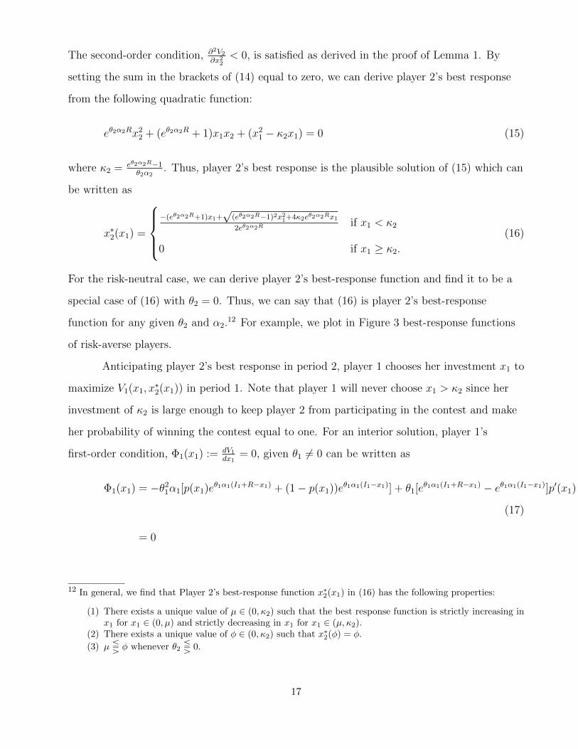
For the risk-neutral case, we can derive player 2’s best-response function and find it to be a

special case of (16) with θ2 = 0. Thus, we can say that (16) is player 2’s best-response

function for any given θ2 and α2.12 For example, we plot in Figure 3 best-response functions

of risk-averse players.

Anticipating player 2’s best response in period 2, player 1 chooses her investment x1 to

maximize V1(x1, x∗2(x1)) in period 1. Note that player 1 will never choose x1 > κ2 since her

investment of κ2 is large enough to keep player 2 from participating in the contest and make

her probability of winning the contest equal to one. For an interior solution, player 1’s

first-order condition, Φ1(x1) := dV1dx1

= 0, given θ1 6= 0 can be written as

Φ1(x1) = −θ21α1[p(x1)eθ1α1(I1+R−x1) + (1− p(x1))eθ1α1(I1−x1)] + θ1[eθ1α1(I1+R−x1) − eθ1α1(I1−x1)]p′(x1)

(17)

= 0

12 In general, we find that Player 2’s best-response function x∗2(x1) in (16) has the following properties:

(1) There exists a unique value of µ ∈ (0, κ2) such that the best response function is strictly increasing inx1 for x1 ∈ (0, µ) and strictly decreasing in x1 for x1 ∈ (µ, κ2).

(2) There exists a unique value of φ ∈ (0, κ2) such that x∗2(φ) = φ.

(3) µ S φ whenever θ2 S 0.

17

x1

x2

BR2

κ2

BR1

xe1

xe2

xs1

xs2

ICe1

ICs1

x2 = x1

(a) θ1 = 0, θ2 = −1, and α2 = 0.6

x1

x2

BR2

xe1 xs1 = κ2

BR1

xe2

ICs1

ICe1

xs2

x2 = x1

(b) θ1 = 0, θ2 = −1, and α2 = 1

Figure 3. Subgame-perfect equilibria in which (a) player 2 participates and (b)does not participate

where p(x1) := x1x1+x∗2(x1)

. If θ1 = 0, the first-order condition for player 1 is given by

−1 +Rp′(x1) = 0. (18)

In the next proposition, we show that player 1’s optimization problem has a unique solution if

θ1α1 is greater than a threshold which has a negative value. Thus, we can say that a

subgame-perfect equilibrium of the game uniquely exists if player 1 is not too risk-averse.

Proposition 6. Consider a sequential two-player contest in which each player’s utility

function has the generalized CARA form and fi(xi) = xi for i = 1, 2. There exists a threshold

ρ < 0 such that a subgame-perfect equilibrium uniquely exists whenever θ1α1 > ρ.


18

In Proposition 6, we prove that a subgame-perfect equilibrium exists for some θ1α1 and

any θ2α2. Specifically, assuming risk neutrality or risk lovingness for player 1 is sufficient but

not necessary for existence and uniqueness of equilibrium. An equilibrium also exists when

player 1 is risk-averse and α1 is small enough.

4.2. Favorites and Underdogs. Dixit (1987) analyzes standard Tullock contest with two

identical players and show that outcomes in simultaneous and sequential contests are identical

when both players are risk-neutral. In other words, Dixit claims that there is neither

first-mover advantage nor disadvantage so there is no incentive for preemptive investment. We

show that Dixit’s theoretical prediction does not hold without the risk-neutrality assumption.

Following Dixit (1987), as player 1 chooses x1 to maximize V1(x1, x∗2(x1)), we have

dV1

dx1

=∂V1

∂x1

+∂V1

∂x2

· dx∗2

dx1

. (19)

In equilibrium of simultaneous contest where x1 = xe1, we know that ∂V1∂x1|x1=xe1

= 0. Since

∂V1∂x2

< 0 for any x1, player 1 will increase/decrease her investment in the sequential contest

from xe1 ifdx∗2dx1|x1=xe1

is negative/positive respectively. Using the results from simultaneous

contests stated in Proposition 5 and the properties of player 2’s best-response function in

Footnote 12, we can derive the following results in sequential contests.


function has the generalized CARA form and fi(xi) = xi for i = 1, 2. We assume that player 1

is not too risk-averse so that a subgame-perfect equilibrium uniquely exists. Let xsi denote

player i’s investment in such an equilibrium.

(1) If |θ1α1| ≤ |θ2α2| and θ2 = −1, then xs1 > xs2.

(2) If |θ1α1| ≥ |θ2α2| and θ2 = 1, then xs1 < xs2.


We find that each player’s attitudes toward risk and downside risk together determine

whether a first-mover or second-mover advantage arises in equilibrium. In particular, if the

19

first mover is less/more-downside-risk-averse and the second mover is risk-averse/loving, then

the first mover will be the favorite/underdog in the contest, respectively.

The first result of Proposition 7 can be illustrated in panel (a) of Figure 3 where we let

R = 1, θ1 = 0, and θ2 = −1, α2 = 0.6. Since |θ1α1| < |θ2α2|, the Nash equilibrium (xe1, xe2) of

simultaneous contest lies below the 45-degree line (i.e., xe1 > xe2) as predicted by Proposition

5. In a sequential contest, player 2’s best response depicted by BR2 becomes a constraint for

player 1’s optimization problem. Specifically, player 1 can maximize her expected utility

V1(x1, x2) by choosing a point on BR2 that is on the lowest indifference curve since a lower

indifference curve corresponds to a higher value of V1(x1, x2). The dashed curve ICe1

represents player 1’s indifference curve corresponding to the simultaneous contest equilibrium.

Since the slope of this indifference curve is zero at (xe1, xe2) while the slope of BR2 at the same

point is negative, player 1 can increase her expected utility by moving along BR2 to the right.

Player 1 will optimally choose xs1 as her investment in period 1 and player 2 will respond by

investing xs2 in period 2 (as a result, xs1 > xs2). Note that the best attainable indifference curve

is labeled ICs1 and (xs1, x

s2) is the tangent point of ICs

1 and BR2.

These findings provide new insights on first-mover advantage and disadvantage in a

sequential contest. Contrasting Dixit’s (1987) seminal result, even when the two players are

identical and no one has an advantage on rent-seeking technology, we find that there is an

advantage of going first or second depending on the players’ risk attitudes. Consider a

two-player sequential contest with θ1 = θ2 6= 0 and α1 = α2 which is a special case of

Proposition 7. We can say that if θ1 = θ2 = −1, i.e., both players are risk-averse, then the

first player will be the favorite to win the contest. On the other hand, if θ1 = θ2 = 1, then the

second player will be the favorite to win the contest. We formally state these immediate

findings in the following corollary.

Corollary 2. Consider a subgame-perfect equilibrium in a sequential two-player contest in

which each player’s utility function has the generalized CARA form with θi = θ, αi = α and

fi(xi) = xi for i = 1, 2. If θ ≶ 0, then xs1 ≷ xs2.

20

In general, an interior solution of a sequential contest does not always exist. As player

2 becomes more risk-averse, θ2α2 decreases and so does κ2. When θ2α2 is low enough, it will

be impossible to find a tangent point on BR2 such that x1 ∈ [0, κ2]. For example, consider the

case where θ1 = 0 and θ2 = −1, α2 = 1 as illustrated in panel (b) of Figure 3. Using (xe1, xe2)

as the starting point, player 1 can increase her expected utility by moving her investment

rightward along BR2 all the way to κ2 yet the slopes of her indifference curve and player 2’s

best-response function are not equalized. Choosing x1 = κ2 stops player 2 from competing in

the rent-seeking contest and maximizes player 1’s expected utility. At this corner solution,

player 2 does not participate in the contest and player 1 wins the rent with probability one.

How low does θ2α2 have to be for player 1 to be able to drive player 2 out of a contest?


function has the generalized CARA form and fi(xi) = xi for i = 1, 2. If θ1 = 0 and

θ2α2 ≤ − 45R

, then xs1 = κ2 and xs2 = 0 in equilibrium.


Proposition 8 suggests that if θ2α2 ≤ − 45R

, player 1 only needs to invest κ2 to secure

the rent. In particular, player 1 will win the rent with probability one and her profit from the

contest will be R− κ2 ¿0.13 Since κ2 is strictly increasing in θ2α2, we can say that as player 2

becomes more risk-averse (i.e., as θ2α2 decreases), the amount of rent-seeking investment in

period 1 needed to keep player 2 out of the contest becomes smaller. Thus, player 1’s profit

rises as player 2 becomes more risk-averse.

5. Conclusion and Discussion

In this paper, we derive conditions for existence and uniqueness of equilibrium in

rent-seeking contests in which players are heterogeneous in both preferences and production

technology. As a special case, we carefully analyze standard Tullock contests in which each

player’s utility function has the generalized CARA form described as in (8). This functional

13We show in Proposition 3 that κ2 < R if and only if θ2 < 0.

21

form allows each player to be risk-averse, risk-neutral, or risk-loving. We find that if the

number of risk-loving players is large enough, rent over-dissipation will occur in equilibrium

and, as a result, all risk-averse players will be crowded out from the contest. On the other

hand, if the number of risk-loving players is less than four, we find that rent over-dissipation

will never occur in equilibrium.

We also analyze the effect of risk attitudes on rent-seeking investment in contests with

two players. If both players move simultaneously, the player who is less downside-risk-averse

will be the favorite to win the rent. If the players move sequentially, a first- or second-mover

advantage may arise in equilibrium depending on both players’ attitudes toward risk and

downside risk. As a special case of this result, even when both players have the same

preferences, the first mover will be the favorite/underdog if they both are risk-averse/loving

respectively.

The generalized CARA utility function can provide more flexibility in explaining

laboratory results under the expected utility framework than linear utility functions usually

assumed in the literature. We finish the paper with a discussion on recent laboratory evidence

on simultaneous and sequential contests. First we analyze experimental findings by Sheremeta

(2011) and Lim, Matros, and Turocy (LMT) in Lim et al. (2014). In particular, we focus on

average investment by participants in simultaneous contests with n = 4 in Sheremeta’s

experiment and n = 4 and 9 in the LMT experiment. In Sheremeta’s experiment, the prize is

120 Experimental Currency Units (ECU) so the symmetric equilibrium prediction when all

players are risk-neutral is 22.5 ECU. Sheremeta finds that on average subjects invest 30.0

ECU which is 7.5 ECU higher than the risk-neutral prediction. Using our generalized CARA

utility function with θ = 1 and α = 0.68, we find that the theoretical prediction for symmetric

equilibrium, according to (11), is 28.0 ECU14 which is 73% closer to the average actual

investment.

14We assume that v(w) = e0.68w where w is in dollar value. The exchange rate for Sheremeta’s experiment is50 ECU per dollar. Our choice of α maximizes rent-seeking investment in symmetric equilibrium given n = 4and R = 120 ECU.

22

Experiment Number of Prize Risk-Neutral Risk-Loving ActualPlayers (ECU) Prediction Prediction (average)

Sheremeta (2011) 4 120 22.5 28.0 30.0Lim, Matros, and 4 1000 188 233 300

Turocy (2014) 9 1000 99 201 326

Table 1. Theoretical predictions and actual investments in simultaneous contests

Our generalized CARA functions also perform better than linear utility functions in

the LMT experiment. Given the prize of 1000 ECU, each experimental subject invests on

average 300 ECU and 326 ECU in contests with n = 4 and n = 9 respectively. While the

risk-neutral predictions for n = 4 and n = 9 are 188 ECU and 99 ECU, our risk-loving

predictions are 233 ECU and 201 ECU.15 Table 1 compares the theoretical predictions based

on risk neutrality and risk lovingness to the actual values from both experiments. Note that

the risk-loving prediction implies rent over-dissipation in equilibrium when n = 9 because the

corresponding investment by all participants is 1809 ECU. Even though our risk-loving

predictions dominate the risk-neutral predictions in both experiments, we can not explain rent

over-dissipation given 4 players as suggested in Proposition 4.16

Finally, we analyze Fonseca’s (2009) sequential contest experiment. We are

particularly interested in strategies chosen by subjects who are followers because there is no

strategic uncertainty when they make a decision; each follower can observe rent-seeking

investment chosen by the leader prior to choosing his optimal investment. Since Miguel

Fonseca kindly allowed us to analyze his data set, we could estimate each follower’s risk

parameters θi and αi according to player 2’s best response given in (16). Using non-linear

least squares optimization, we find that all followers are risk-loving, that is, for all 15 subjects

in the Seqsym treatment, θi = 1 for all i. The estimated value of αi ranges from 0.19 to 3.87

15We assume that v(w) = e0.16w and v(w) = e0.30wwhere w is in dollar value for contests with n = 4 and n = 9respectively. The exchange rate in the LMT experiment is 100 ECU per dollar.16For contest experiments with fewer participants, other psychological effects such as utility of winning andoptimism discussed in Sheremeta (2013) may help explain rent over-dissipation. For example, if we adopt theadditive utility of winning assumption suggested in Sheremeta (2010), we can jointly estimate our preferenceparameters, θ and α, and Sheremeta’s utility of winning by letting ri = R+ ωi, where ωi is player i’s utility ofwinning the rent. When ωi is large enough, rent over-dissipation outcome can be obtained in a 4-player contest,but this approach is beyond the scope of this paper.

23

−2 0 2 4 6 8 100.2

0.4

0.6

0.8

1

θiαi

SSR θiαi = 0

θiαi = 3.87

(a) Sum of squared residuals given θiαi

0 50 100 150 200 250 300

50

100

150

200

θiαi = 3.87

θiαi = 0

x1

x2

(b) Best-response functions

Figure 4. Estimation of θiαi for i = 10 in Session 1 of Fonseca’s experiment

with a mean of 2.59 and a median of 2.93.17 We plot sum of squared residuals (SSR) given

θiαi for subject number 10 from session 1 in panel (a) of Figure 4. The value of θiαi that

minimizes the SSR is 3.87, the highest estimated value of θiαi of all 15 subjects. We plot this

subject’s actual responses along with best-response functions given θiαi = 0 and θiαi = 3.87 in

panel (b). The dashed best-response curve corresponding to risk-loving attitude seems to fit

the observed data much better than the solid best-response curve which is based on the

risk-neutrality assumption.

17We assume that vi(w) = eαiw where w is in dollar value. The exchange rate in the Fonseca’s experiment is1000 ECU for 1.2 pounds or approximately 2.4 dollars.

24

CHAPTER 2. FREE RIDERS AND OPTIMAL PRIZE IN PUBLIC GOOD

FUNDING LOTTERY

1. Introduction

Lottery is an efficient and popular fundraising mechanism. In 2016, Americans

purchased 73 billion dollars of lottery tickets in forty-four states and nearly one-third of the

amount was able to fund education and other social programs.18 In theory, it is well known

that a voluntary contribution mechanism (VCM) leads to public good under-provision

because of the positive externality associated with the public good. Morgan (2000) shows that

using lottery to finance a public good is a more effective mechanism since a player’s lottery

purchase causes negative externality by reducing other players’ probabilities of winning. In

addition, Morgan and Sefton (2000) provide experimental evidence to support this theoretical

prediction and show that each player’s incentive to contribute is driven by the benefit from

consumption of the public good and also the joy of gambling.19

Even though many studies have extended Morgan’s (2000) framework in various

directions and alternative schemes have been proposed,20 the effects of risk preferences on the

lottery mechanism are rarely analyzed in the literature.21 Specifically, most researchers adopt

Morgan’s (2000) assumption of quasi-linear utility so that each player’s marginal utility from

private consumption is constant. Thus, the marginal utility of income is the same regardless

18See La Fleur’s 2017 World Lottery Almanac.19Experimental evidence about the efficiency of the lottery mechanism can also be found in Dale (2004) andLandry et al (2006).20See Goeree et al (2005), Lange et al (2007a), Maeda (2008), Gorazzini et al (2010), Kolmar and Wagener(2012), Faravelli and Stancab (2012, 2014), Franke and Leininger (2014), Kolmar and Sisak (2014), Bos (2011,2016), Damianov and Peeters (2018).21Two exceptions are Lange et al (2007b) and Duncan (2002). Lange et al (2007b) show that the lotterymechanism does not always dominate VCM given sufficient risk aversion. While Morgan (2000) shows thatincreasing the lottery prize will always increase public good provision, Duncan (2002) illustrates by an examplethat there may exist a finite public-good-maximizing prize under risk aversion.

25

of whether he is a lottery winner. In this paper, we propose a framework that allows for

concavity in utility functions with respect to both private and public good consumption.

We generalize Morgan’s public good game by allowing for heterogeneous risk-averse

players. First, we derive a necessary and sufficient condition for existence and uniqueness of

equilibrium with positive provision of a pure public good. Such an equilibrium exists if and

only if the number of players who are not too risk averse is large enough. Second, we find that

free riders, if they exist, are players who are either more risk-averse or have lower valuations on

the public good. Among those who contribute, we show that a player’s contribution decreases

with the degree of risk aversion and increases with the valuation on the public good.22

We also analyze the effects of redistribution of players’ risk preferences and valuations

on the public good. Specifically, we consider first-order redistributions.23 Warr (1982) and

Bergstrom et al (1986) examine the effect of a redistribution of income on the provision of a

public good. Although Warr (1982) finds that a redistribution of income will not affect the

provision of a public good, Bergstrom et al (1986) argue that Warr’s (1982) result will not

hold if the redistribution changes the set of contributors. Given a distribution of income, we

find that any first-order redistribution of contributors’ degrees of risk aversion and valuations

on the public good can change the provision of the public good, even though there is no

change in the set of contributors.

Given a set of homogeneous players, we derive the amount of public-good provision in

equilibrium as a function of lottery prize, the number of players, each player’s preference

parameters. Like Morgan (2000), we find that equilibrium public good provision is increasing

with the number of players. However, when players are risk-averse, there is a finite upper

limit for the public good provision even when the number of players becomes infinitely large.

22Andreoni (1988) shows that only players with high demand of the public good would bear the burden inthe provision of a public good in a large group, which confirms Olson’s (1965) claim about the group memberasymmetry. However, our results demonstrate that more risk-averse players can take advantage of less risk-averseplayers, even though they have the same valuation on the public good.23We use the concepts of first-order stochastic dominance to characterize the change of the distribution.Specifically, first-order redistribution means the distribution after the change is first-order stochasticallydominates the original one.

26

Another strand of literature has dealt with the improvement of the lottery design.

Lange et al (2007b) investigate the multiple-prize lottery design. Goerg et al (2016) propose a

two-stage lottery procedure to increase the public good provision. Carpenter and Matthews

(2017) find that a contest success function with convex technology can make the lottery

mechanism more efficient. In this paper, we derive the lottery prize that maximizes the public

good provision for a given number of players. Nonetheless, this prize does not maximize each

player’s expected utility. We find that the public-good-maximizing prize is always greater

than the expected-utility-maximizing prize and both prizes converge as the number of players

approaches infinity.

The paper is organized as follows. Section 2 proves existence and uniqueness of

equilibrium and provides the condition for the lottery mechanism to outperform VCM.

Section 3 presents comparative statics results on each player’s participation and contribution.

Section 4 analyzes public good provision in equilibrium and optimal lottery design. Section 5

concludes.

2. Existence and Uniqueness of Equilibrium

Consider a game in which n ≥ 2 players simultaneously choose an amount of lottery

purchase. One of the players will be randomly selected to be the lottery winner and receive a

fixed prize, R > 0. Let xi be player i’s wager for i = 1, ..., n. The probability that player i

wins the prize is

pi =xi

xi +X−i=xiX

(20)

where X =∑n

i=1 xi and X−i = X − xi. If player i does not buy any lottery, his probability of

winning the prize will be zero. If xi = 0 for all i, pi in (20) is not defined so we impose that

pi = 0 for all i. Since ∂pi∂xi

> 0 (when X−i > 0) and ∂pi∂X−i

< 0 (when xi > 0), player i’s

probability of winning is strictly increasing in his own lottery purchase and decreasing in

other players’ lottery purchases. The lottery organizer uses the profit from selling lottery

27

tickets to finance a pure public good so that the amount of the public good provided is

G = X −R > 0.24 We assume that each player’s utility function has the following form.

Assumption 3. Player i’s utility function is given by

ui(wi, G) = −e−[αiwi+hi(G)] (21)

where wi is his final wealth (or private good consumption) and G is his public good

consumption. We assume that αi > 0, hi(0) = 0, 0 < h′i(G) < αi, and h′′i (G) ≤ 0 for all G.

The utility function in Assumption 3 is strictly increasing and concave in both wi and

G. Given 0 < h′i(G) < αi, we have ∂ui(wi,G)∂wi

> ∂ui(wi,G)∂G

> 0, that is, each player’s marginal

utility from private consumption is always greater than marginal utility from the public good.

Thus, no public good will be provided under VCM. Player i’s absolute measure of risk

aversion with respect to wi is a constant αi for any level of wi and G. Note that, for players i

and j, αi and αj can take different values and hi and hj are allowed to be different functions.

Morgan (2000) allows the lottery organizer to tolerate a deficit financing of an amount

δ, i.e., the lottery proceeds as usual if X −R < −δ, otherwise it is called of. He shows in

Lemma 4 of his paper that given a quasilinear utility function, ui(wi, G) = wi + hi(G), and

any δ > 0, each player has an incentive to increase his wager so that X −R = −δ even though

G = 0. Thus, under Morgan’s framework, the lottery is never called off in equilibrium. This

result does not hold for the utility functions in Assumption 3. In particular, players with a

utility function in (21) will have such an incentive only when δ is large enough.25 Since we are

not interested in an equilibrium that is dependent on δ, we focus on equilibrium in which

X −R > 0 so that the public good provision is strictly positive.

24In Morgan (2000), G = max{X −R, 0}. In this paper we only consider the cases where a positive amount ofthe public good is provided in equilibrium, not when the lottery profit is negative.25Following Lemma 4 in Morgan (2000) but using the utility funciton in (21), we find that player i has an

incentive to increase his wager so the lottery is not called off when 1−e−αixixi

< 1−e−αiRR−δ . Since f(x) := 1−e−αix

x

is strictly positive and strictly decreasing for x > 0, we find that such an inequality holds for xi < R only whenδ is large enough.

28

Given an initial level of wealth Ii, player i chooses xi to maximize

Ui(xi|X−i) =xi

xi +X−i{−e−[αi(Ii−xi+R)+hi(G)]}+

X−ixi +X−i

{−e−[αi(Ii−xi)+hi(G)]}. (22)

Note that Ui(0|0) is undefined but it is not relevant since player i’s best response to X−i = 0

is the smallest possible positive value of xi. The first-order condition for utility maximization

is given by

dUidxi

=e−[αi(Ii−xi)+hi(G)]

X2{X−i(1− e−αiR)− [αi − h′i(G)](xie

−αiR +X−i)X} = 0 (23)

which is equivalent to

X−iX

(1− e−αiR)− [αi − h′i(X −R)]

(xiXe−αiR +

X−iX

)X = 0. (24)

Let x∗i denote a nonnegative value of xi satisfying the first-order condition. Since

d2Uidx2i|xi=x∗i < 0, there exists at most one x∗i . If dUi

dxi|xi=0 < 0, then we know that the value of xi

satisfying the first-order condition is negative and, therefore, player i will not buy any lottery.

By substituting xiX

= si and X−iX

= 1− si in (24), player i’s probability of winning can

be written as a function of X:

si(X) = max

{1− e−αiR − [αi − h′i(X −R)]X

(1− e−αiR){1− [αi − h′i(X −R)]X}, 0

}. (25)

Following Cornes and Hartley (2003 and 2005), we call si(X) player i’s share function which

is the probability of winning the prize given all other players’ wagers and his own best

response. If dUidxi|xi=0 ≤ 0, then the optimal choice of xi will be zero and so is si(X). Let κi be

the value of X such that the numerator in (25) is equal to 0, that is,

[αi − h′i(X −R)]X = 1− e−αiR. (26)

We find that dUidxi|xi=0 ≤ 0 when X ≥ κi. The left-hand side of (26) is strictly increasing in X

and it is equal to zero when X = 0. Since the right-hand side of (26) is positive, κi is strictly

29

positive. We call κi player i’s participation threshold because player i will not buy any lottery

if X ≥ κi, or equivalently, X−i ≥ κi.

Lemma 3. Suppose that Assumption 3 holds. Player i’s share function is given by

si(X) =

1−e−αiR−[αi−h′i(X−R)]X

(1−e−αiR){1−[αi−h′i(X−R)]X} if X ∈ (0, κi)

0 if X ≥ κi

(27)

where κi satisfies (26). The share function has the following properties:

(1) si(X) is continuous in X for X > 0;

(2) limX→0 si(X) = 1 and limX→κi si(X) = 0;

(3) si(X) is strictly decreasing for all X ∈ (R, κi).

Proof. See Appendix B. �

We know that there is a participation threshold, κi > 0, for player i = 1, ..., n. Given

X > κi, player i will not buy any lottery ticket. It follows that in equilibrium, X must be less

than max{κ1, ..., κn}. Now we consider the properties of each player’s share function

described in Lemma 3. Since si(X) is continuous and strictly decreasing in X for X ∈ (R, κi),

the sum of all shares,∑n

i=1 si(X), is also continuous and strictly decreasing in X for

X ∈ (R, κm) where κm = max{κ1, ..., κn}. We also know that limX→κm∑n

i=1 si(X) = 0

because limX→κi si(X) = 0 for all i. If∑n

i=1 si(R) > 1, then there must be a unique value of

X > R such that∑n

i=1 si(X) = 1, i.e., an equilibrium of the game. We call such a value Xe.

Player i’s equilibrium investment in the lottery is xei = si(Xe)Xe. The provision of the public

good is Ge = Xe −R > 0. However, if∑n

i=1 si(R) ≤ 1, there is no equilibrium such that

Xe > R. Therefore, no public good will be provided in equilibrium. In this case, the lottery

mechanism fails to increase the public good provision relative to VCM.

Proposition 9. Suppose that Assumption 3 holds. There exists a unique equilibrium with

Ge > 0 if and only if∑n

i=1 si(R) > 1.

Proof. See the above argument. �

30

Proposition 9 provides a necessary and sufficient condition for the lottery mechanism

to outperform VCM, since no public good will be provided in the latter. In general, we may

or may not have∑n

i=1 si(R) > 1 so that Ge > 0 in equilibrium. Nevertheless, we can say that

if there are enough players whose participation thresholds are greater than R, then∑n

i=1 si(R)

will be greater than 1 and there will be an equilibrium with a strictly positive amount of

public good provision.

3. Comparative Statics

In order to derive analytical results and comparative statics, we assume a specific

functional form of hi(G) that satisfies Assumption 3. Suppose that hi(G) = βiG so

ui(wi, G) = −e−(αiwi+βiG) (28)

and that αi > βi > 0.26 Player i’s preferences depend on two parameters αi and βi which

represent his Arrow-Pratt absolute measures of risk aversion with respect to wi and G

respectively. We can interpret βi as player i’s valuation of the public good when β ∈ (0, 1).27

Given hi(G) = βiG, the share function si(X) in (27) can be written as

si(X) =

κi−X

κi−(1−e−αiR)Xif X ∈ (0, κi)

0 if X ≥ κi.

(29)

where

κi =1− e−αiR

αi − βi. (30)

Since we focus on equilibrium where a positive amount of the public good is provided, i.e.,

Xe > R, players whose participation threshold is not greater than R will always free ride in

such an equilibrium. According to (29), we find that si(R) < 1 for all i. Thus, we need to

26In addition to the linear functional form used in this section, we let hi(G) = βiln(G+ 1) and derive parallelresults in the Appendix B.27Since ∂u

∂G = βe−(αiwi+βiG) and ∂2u∂β∂G = (1 − β2

i )e−(αiwi+βiG), player i’s marginal utility of G is strictly

increasing with βi when βi ∈ (0, 1).

31

impose that the number of players with κi ≥ R is large enough so that∑n

i=1 si(R) > 1 which

implies that an equilibrium with Xe > R exists. We have already proved in Proposition 9 that

such an equilibrium is unique. Given (30), we find that κi ≥ R if and only if βi is larger than

a threshold specified in the following corollary.

Corollary 3. Suppose that ui(wi, G) = −e−(αiwi+βiG) and αi > βi > 0. There exists a unique

equilibrium with Ge > 0 if and only if the number of players such that

βi > αi −1− e−αiR

R. (31)

is large enough.

Example 4: Let R = 0.5. Suppose that there are 2 identical players with αi = 1 and

βi = 0.55. We find that 2si(0.54) = 1 so Xe = 0.54 and Ge = 0.54− 0.5 = 0.04. See Xe1 in

Figure 5.

Example 5: Let R = 0.5. Suppose that there are 2 identical players with αi = 1.5 and

βi = 0.75. We find that 2si(R) = 0.93 < 1 so an equilibrium with Ge > 0 does not exist. If

n = 3, then 3si(0.57) = 1 and Ge = 0.57− 0.5 = 0.07. See Xe2 in Figure 5.

0.5 0.55 0.6 0.65 0.7 0.75 0.8 0.85 0.90

0.1

0.2

0.3

0.4

0.5

0.6

0.7

αi = 1, βi = 0.55

αi = 1.5, βi = 0.75

Xe2Xe

1 Xe3

X

si

Figure 5. Share functions given ui(wi, G) = −e−(αiwi+βiG) and R = 0.5

32

Next, we analyze comparative statics of κi.

Proposition 10. Suppose that ui(wi, G) = −e−(αiwi+βiG) and αi > βi > 0. Player i’s

participation threshold, κi, is strictly decreasing in αi and strictly increasing in βi. Thus,

players with larger αi or smaller βi are more likely to free ride in equilibrium.


When X > κi, player i will not buy any lottery. Proposition 10 suggests that players

who are more risk-averse (larger αi) or have lower valuations on the public good (smaller βi)

are more likely to free ride in equilibrium. Olson (1965) claims that the burden of public good

provision is disproportionately borne by players with high demand of it. In contrast, we find

that less risk-averse players bear more of the cost of the public good because gambling is more

tolerable to them, while more risk-averse players free ride despite the fact that they may have

a larger valuation of the public good. In the following example, we show that it is possible for

players with a larger βi to free ride in equilibrium because they are much more risk averse.

Example 6: Let R = 0.5. Suppose there are two types of players: a type-1 player has αi = 1

and βi = 0.55 while a type-2 player has αi = 1.5 and βi = 0.75. Let nt denote the number of

type-t players. Suppose that n1 = 5 and n2 = 2. We find that Xe = 0.76 so Ge = 0.26. Since

type-2 players have a participation threshold κi = 0.704 < Xe, they will not contribute even

though their βi is larger. See Xe3 in Figure 5.

For all players who do not free ride in equilibrium, we show in the following

proposition that player i’s contribution is decreasing in αi and increasing in βi.

Proposition 11. Suppose that ui(wi, G) = −e−(αiwi+βiG) where αi > βi > 0. If player i’s

lottery purchase in equilibrium, xei , is strictly positive, then xei is strictly decreasing in αi and

strictly increasing in βi.


33

Next, we focus on the distributions of player types represented by αi and βi. Suppose

that there are two groups with the same number of players and group 1’s distribution of

degrees of risk aversion first-order stochastically dominates group 2’s. That is, we can derive

group 1’s distribution by a rightward shift from group 2’s cumulative distribution function so

we can say that, for any α, group 1 has more players with αi > α than group 2. Due to

Proposition 10, for any κ, group 1 has more players with κi < κ than group 2. Therefore the

participation rate in equilibrium of group 1 is less than or equal to that of group 2. Moreover,

Proposition 11 suggests that as some players become more risk-averse due to the

redistribution of αi, the amount of public good provided in equilibrium of group 1 will be

lower than or equal to that of group 2. Using the same analogy, we obtain the opposite results

for the effects of a redistribution of βi. We now state the following corollary. Let qe denote the

corresponding participation rate of players in equilibrium.

Corollary 4. Suppose that ui(wi, G) = −e−(αiwi+βiG) where αi > βi > 0. Let Fα and Fβ be

distributions of αi and βi respectively.

(1) If the distribution of αi becomes F ′α which first-order stochastically dominates Fα while

Fβ does not change, then both Ge and qe weakly decrease.

(2) If the distribution of βi becomes F ′β which first-order stochastically dominates Fβ while

Fα does not change, then both Ge and qe weakly increase.

Bergstrom et al (1986) show that a redistribution of wealth could only significantly

affect the provision of public good if the set of contributors is changed. Nevertheless, Corollary

4 suggests that any first-order redistribution of either degrees of risk aversion with respect to

wealth or valuations on the public good will change the provision of public good even though

the participation rate may stay the same and there is no change of the set of contributors.

Finally, we consider a special case where αi = α and βi = β for i = 1, ..., n. It follows

that the participation threshold κi is the same for all players, that is,

κi = κ :=1− e−αR

α− β(32)

34

for all i. By setting si = 1n, we obtain total wagers in equilibrium as a function of n and R,

Xe(n,R) =κ(n− 1)

e−αR + n− 1(33)

and the corresponding amount of the public good Ge(n,R) = Xe(n,R)−R.

First, we examine the effectiveness of the lottery mechanism as n increases. The

following proposition presents the effect of group size on the public good provision.

Proposition 12. Suppose that ui(w,G) = −e−(αw+βG) where α > β > α− 1−e−αRR

for

i = 1, ..., n. For a given R > 0, there exists a unique equilibrium with Ge(n,R) > 0 if and only

if

n > 1 +(α− β)Re−αR

1− e−αR − (α− β)R. (34)

In such an equilibrium, we find that

(1) ∂Ge(n,R)∂n

> 0.

(2) limn→∞Ge(n,R) = κ−R > 0.


Proposition 12 demonstrates that public good provision is increasing in group size,

while there is an upper bound for the quantity of the public good that can be funded by

lotteries even when n is infinitely large. This result suggests that we will never observe the

strong form of Olson’s group-size paradox, which states that the public good provision is

decreasing in the number of players and public good cannot be provided for large groups.28

4. Optimal Lottery Prize

In order to derive an optimal prize as a function of each player’s preference parameters

and the number of players, we assume that all players are homogeneous and have the

following utility function:

ui(w,G) = −e−(αw+βG) (35)

28See Olson (1965). See Sandler (2015) and Pecorino (2015) for comprehensive reviews of Olson’s (1965) work.

35

with α > β > 0 for i = 1, ..., n. In this section, we analyze the value of R chosen by the lottery

organizer. The following proposition provides a sufficient condition for existence of R such

that Ge > 0.

Proposition 13. Suppose that ui(w,G) = −e−(αw+βG) where α > β > αn

for i = 1, ..., n. For a

given n ≥ 2, there exists R > 0 such that Ge(n,R) > 0 for all R ∈ (0, R).


We assume henceforth that β > αn

so there exists R such that Ge > 0. The optimal

prize (R∗) that maximizes the public good provision in equilibrium is provided in the

following proposition.

Proposition 14. Suppose that u(w,G) = −e−(αw+βG) and α > β > αn

. We find that

R∗(n) :=1

α

{ln

[2(1− β

α

)n− 1

]− ln

[n− 2

(1− β

α

)−

√n2 − 4n

(1− β

α

)]}(36)

maximizes the public good provision in equilibrium and

(1) ∂R∗(n)∂n≷ 0 if and only if β

α≶ 1

2+ 1

4n.

(2) limn→∞R∗(n) = 1

αln(

αα−β

).

(3) limn→∞Ge(n,R∗(n)) = 1

α

[β

α−β − ln(

αα−β

)].


Proposition 14 indicates that the public-good-maximizing prize R∗ is either increasing

or decreasing in n, depending on the ratio between α and β. Given an equilibrium with

Ge > 0, Proposition 14 implies that ∂R∗

∂n> 0 if 1

n< β

α< 1

2+ 1

4n, while ∂R∗

∂n< 0 if β

α> 1

2+ 1

4n.

Besides, the public-good-maximizing prize R∗ will always be finite even when the number of

players becomes infinitely large, and so is the maximized public good provision.

The following proposition provides the optimal prize R that maximizes expected utility

of the players.

36

Proposition 15. Suppose that u(w,G) = −e−(αw+βG) and α > β > αn

. We find that

R(n) =1

α

{ln[2(α− β)2]− ln

[√(n− 1)2αβ

[(n2 − 6n− 3)αβ + 4nβ2 + 4α2

]−

(n− 1)[(n− 3)αβ + 2β2]]}

(37)

maximizes each player’s expected utility and

(1) ∂R(n)∂n

> 0.

(2) R∗(n)− R(n) > 0 for all n.

(3) limn→∞R∗(n)− R(n) = 0.


From Proposition 13, we know that β > αn

is the sufficient condition for existence of

the prize such that the corresponding value of Ge is strictly positive. Therefore, Proposition

15 suggests that the expected-utility-maximizing prize R is strictly increasing in the number

of players for any equilibrium with Ge > 0. We also find that the public-good-maximizing

prize is always greater than the expected-utility-maximizing prize given any finite size of

group. The larger the difference between these two prizes, the higher the utility cost by

choosing R∗. Nevertheless, R∗ and R converge to the same finite value when n becomes

infinitely large. Thus, the utility cost of choosing R∗ is lower for a larger group. The following

example illustrates the relation between R∗ and R.

Example 7: Let α = 1 and β = 0.55. Since β > αn, for all n ≥ 2, there exists R such that the

provision of the public good is positive for all n ≥ 2. Moreover, we know that βα< 1

2+ 1

4nand

so both R∗ and R will be increasing in n. Figure 6 (a) illustrates the changes of R∗ and R

when n increases. Although R∗ is above R, they are moving closer when n increases. Figure 6

(b) shows that the maximum public good provision G∗ is increasing in n and converges to a

finite value. The public good provision G corresponding to the expected-utility-maximizing

prize is always less than G∗. Furthermore, the difference between G∗ and G is negligible when

n is sufficiently large.

37

2 3 4 5 6 7 8 9 100

0.2

0.4

0.6

0.8R∗

R

n

R

(a) R∗ and R with α = 1 and β = 0.55

2 3 4 5 6 7 8 9 100

0.1

0.2

0.3

0.4

G∗

G

n

G

(b) G∗ and G with α = 1 and β = 0.55

Figure 6. Optimal lottery prize and public good provision given n

5. Conclusion

In this paper, we derive a necessary and sufficient condition for Morgan’s lottery

mechanism to outperform voluntary contribution mechanism in public good financing when

players are risk averse. While Pecorino and Temimi (2007, 2012) show that rivalry can result

in a lottery mechanism breakdown, we show that risk aversion may cause the same result. By

allowing players to have different degrees of risk aversion and different valuations on a public

good, we find that the players who are more risk averse and place less value on the public

good contribute less and are more likely to free ride in equilibrium.

We also show that the amount of public good in equilibrium can be affected by a

first-order redistribution of either degrees of risk aversion or valuations on the public good

and will be increasing in group size. Thus, we never observe the strong form of Olson’s

group-size paradox in the lottery mechanism even though players are risk averse. However,

contrasting Morgan’s risk-neutral framework, we find that there is an upper bound for the

38

amount of public good that can be provided in equilibrium even when group size approaches

infinity. In other words, we cannot keep increasing the lottery prize in order to increase the

amount of public good provision.

We also provide new insights for optimal lottery design. We derive an

expected-utility-maximizing prize, show that it depends on both number of players and each

player’s risk attitude, and find that it is always smaller than public-good-maximizing prize.

Therefore, a lottery organizer whose objective is to maximize public good provision will

always over-provide the public good.

39

CHAPTER 3. RISK AVERSION IN CLASS ACTION SUITS

1. Introduction

A class action allows a group of plaintiffs harmed by the same defendant to bring a

collective claim to the court. While a class action suit can be initiated by a representative

plaintiff, the representative plaintiff has to bear the cost to initiate the class action. Thus,

plaintiffs who join the class later free-ride on the effort spent by the initiator. Free-riding

gives an incentive for potential plaintiffs to wait someone else to initiate a class action.

Therefore, the initiator is usually the plaintiff who can obtain largest benefits from the class

action. Marceau and Mongrain (2003) find that a plaintiff who has the lowest damage claim

has an incentive to initiate the class action if complete damage averaging is applied. In this

case, this plaintiff can be overcompensated if plaintiffs with higher damage claims join the

class. If plaintiffs file a suit against the defendant in a sequence, Deffains and Langlais (2011)

find plaintiffs who do it later can benefit from the positive informational externalities

produced by previous trials. Therefore, the first plaintiff in the sequence has a strong

incentive to initiate the class action to internalize informational externalities.

Alternatively, the class action can be initiated by a counsel who receives a proportion

of the total compensation if plaintiffs either prevail at trial or enter into a pretrial settlement.

This charge is called a contingent fee. This approach does not suffer from free-riding issues

among plaintiffs because the counsel not only bears the legal cost but also takes the risk in

the litigation process. For plaintiffs, letting a counsel lead the class action avoids exposure to

litigation risk but may also lower their expected payoffs. However, allowing a counsel to

initiate a class action can lead to principal-agent problems. Opportunistic counsels may

maximize their profits at the expense of the represented class members. Furthermore, a

majority of class members have no incentives to monitor the behavior of the class counsel. For

40

these reasons, in class action suits the court typically is responsible for ensuring that any

compensation/settlement is fair for all class members.

Contingent fee is commonly used in real class action lawsuits and advertised as a

method to overcome principal-agent problems. Lynk (1990, 1994) discusses the efficiency of

contingent fee in class action lawsuits. Klement and Neeman (2004) analyze the optimal

contingent payment scheme for the class counsel to maximize the class members’ expected

recovery. Nevertheless, Sacconi (2011) argues that the class counsel does not respect the

“fiduciary obligations” under contingent fee payment structure. Emons (2006) finds that

contingent fee encourages the class counsel to take risky litigation plans even though

risk-averse plaintiffs prefer safer plans. Emons (2006, 2007) discusses the benefits of using a

conditional fee as an alternative payment structure to contingent fee. In both payment

structures, the class counsel only receives a payoff if the plaintiff party prevails at trial.

However, conditional fee does not depend on the total compensation, which can discourage

the counsel to take unnecessary risk to seek a higher stake.

Although the effects of heterogeneity of plaintiffs’ damage claims on the formation of a

class action and the efficiency of contingent fee have been extensively analyzed in the

literature, the effect of plaintiffs’ risk preferences is still a field that needs further exploration.

Besides financial unfeasibility, risk aversion can also stop plaintiffs from suing the defendant

individually. The more risk-averse the plaintiffs, the less incentive for them to take the

litigation risk to fight against the defendant. A class action initiated by a risk-neutral counsel

can transfer the legal risk from plaintiffs in the class to the counsel and thus encourage

risk-averse plaintiffs to join the class.

This paper mainly examines the effects of the heterogeneity of plaintiffs’ risk aversion

on the formation of the class and the role of a self-interested class counsel in the class action

lawsuit. I model the legal process as a three-stage game. First, plaintiffs decide whether to

join the class. Any plaintiff can opt out and file a suit against the defendant individually.

Second, the class or an opt-out plaintiff can negotiate with the defendant for a pretrial

settlement. If the settlement offer is accepted, the game ends. Otherwise, the game moves to

41

the last stage. In this stage, all disputing parties go to court to litigate the case. In the

literature, it is common to assume that the court awards the correct compensatory damages

to plaintiffs, which implies that the defendant is always found guilty at trial. Nonetheless,

Farmer and Pecorino (1999) use the rent-seeking contest model to examine the endogenous

legal expenditure. In this case, the outcome of a trial depends on both disputing parties’ legal

investment. This paper also applies Tullock’s (1980) rent-seeking contest to model the

litigation process. I find that plaintiffs’ investment and probability of winning are decreasing

in the degree of risk aversion in individual suits. It implies that more risk-averse plaintiffs

have less incentive to sue the defendant individually.

I find that the defendant prefers settling the case in both a class action lawsuit and an

individual suit. Less risk-averse plaintiffs receive higher settlement offers in individual suits

than more risk-averse plaintiffs. If the defendant has perfect information, without a class

counsel, more risk-averse plaintiffs join the class while less risk-averse plaintiffs opt out, which

is similar to the adverse selection situation in Che (1996). In the same information structure,

a self-interested counsel cannot change the structure of the class but can punish the defendant

more financially and make class members (i.e. more risk-averse plaintiffs) better off. In an

environment that the defendant has incomplete information, a class action initiated by a

counsel cannot be formed if there are enough less risk-averse plaintiffs. Nonetheless, a grand

class that all plaintiffs join can be formed if they are all risk-averse enough, even though the

class counsel is self-interested. This result supports Che’s (2002) argument that a

self-interested representative may be preferred by plaintiffs if the representative bears the

legal cost.

This paper is organized as follows. Section 2 sets up the model and analyzes the

optimal decisions for disputing parties at trial and pretrial settlement negotiation. Section 3

studies the equilibrium formation of the class action when the defendant has perfect

information. Section 4 examines the informational effects on the formation of the class and

the role of a self-interested class counsel. Section 5 concludes.

42

2. The Model

Consider an incident where n plaintiffs are harmed by a single risk-neutral defendant

with n ≥ 2. Each plaintiff’s damage claim against the defendant is r. For i = 1, ..., n, plaintiff

i has an initial wealth Ii and preferences represented by the following utility function.

Assumption 4. Plaintiff i’s utility function is

ui(wi) = −e−αiwi (38)

for all wi, where wi indicates plaintiff i’s final wealth.

The above utility function is strictly increasing and concave in wi. As a result, all

plaintiffs are risk averse in this model. αi represents the degree of risk aversion. Moreover,

plaintiffs have heterogeneous risk preferences because αi and αj are allowed to be different for

plaintiff i and plaintiff j.

The game has three stages. At the first stage of the game, each plaintiff has two

choices. Each plaintiff can choose to file a suit against the defendant individually. Second, he

can join a class action suit that sues on behalf of all class members. All plaintiffs make their

decisions simultaneously. For example, if q ≥ 0 plaintiffs choose to join the class action, n− q

plaintiffs will opt out, which implies that they sue individually. If q ≥ 2, the class action is

formed. A class action is initiated by a self-interested counsel who bears all the legal cost

associated with the class action lawsuit and charges a contingent fee in the event of winning

at trial or successful pretrial settlement. Specifically, the contingent fee is a proportion

γ ∈ (0, 1) of the total compensation or settlement for all class members.

Three assumptions are made in the first stage of the game. First, plaintiffs voluntarily

join the class action and all plaintiffs are eligible to become members of the class. There is no

legal obligation for any plaintiff to join the class, while no one is excluded from the class

before the formation of the class. Second, at most one class action can be formed. Third, the

43

membership of the class becomes binding once the class is formed. In other words, no one can

opt out or opt in after the formation of the class action.29

At the second stage of the game, an opt-out plaintiff or the class has a chance to

negotiate a pretrial settlement with the defendant. The defendant makes a take-it-or-leave-it

offer to either an opt-out plaintiff or the class. An opt-out plaintiff either accepts or rejects

the settlement offer. The self-interested counsel makes the decision about acceptance or

rejection for the class.30 If the opt-out plaintiff accepts the settlement offer, the settlement

will be paid and the game ends. In the case of a class action initiated by a self-interested

counsel, the counsel receives a proportion γ of the total settlement and the remaining payoff is

divided equally among the class members. If the offer is rejected, a trial will occur in the

following stage of the game.

In the third stage of the game, all parties go to court. A trial can happen either

between an opt-out plaintiff and the defendant or between a class and the defendant.

American rule is applied in litigation. That is, each disputing party pays its own legal cost. In

a class with a self-interested counsel, the counsel takes all legal cost. Thus, in this case, the

litigation is financially free for class members. I use Tullock’s contest to model the litigation

process. The probability that each party prevails at trial depends on its own legal investment

(cost) and the investment (cost) of the other party that it is against.

Assumption 5. Disputing party i’s probability of prevailing at trial is given by

pi =ci

ci + cj(39)

where ci is party i’s legal investment and cj is the investment from the other party at trial.

If the plaintiff party (either an opt-out plaintiff or a class) prevails at trial, the

defendant pays the compensation and incurs a loss of r + cD in an individual suit against an

29In real practice, plaintiffs have to make their decisions about whether to opt out by the deadline imposed bythe court.30In a real class action lawsuit, members in the class have the option to object to a proposed settlement offer.However, the objection rates across different types of class action are usually very low. See Eisenberg and Miller(2004).

44

opt-out plaintiff or a loss of nr+ cD in a class action lawsuit, where cD is the defendant’s legal

investment. An opt-out plaintiff i recovers r − ci. In a class action with a self-interested

counsel, the counsel’s profit is γnr − cR, where cR is the counsel’s legal investment, in the

event of winning at trial. As a result, each class member receives (1− γ)r. I assume that

there is no spillover effect among lawsuits.31 That is, a successful settlement or prevailing at

trial for the class does not affect the settlement negotiation or probability of winning at trial

for an individual suit between an opt-out plaintiff and the defendant.

The risk neutrality of the defendant and the counsel, the contingent fee, and each

plaintiff’s damage claim (r) are public information. For the knowledge about plaintiffs’ risk

preferences, I consider two different information structures. In the first structure, each

plaintiff’s risk preferences are known to the defendant. In the second information structure,

each plaintiff’s risk preferences are private information and unknown to other plaintiffs and

the defendant. In reality, perfect information about risk preferences may not be realistic.

However, studying the first structure can help us build benchmarks that can be used to

compare with the results under incomplete information environment (second structure) and

show the informational effect.

I use backward induction to analyze the equilibrium of the game. In the rest of this

section, I analyze the second and the third stages of the game for both an individual suit and

a class action lawsuit. In the next two sections, I examine the equilibrium behavior in the first

stage.

Suppose that the defendant knows plaintiff i’s risk preferences. In an individual suit,

plaintiff i’s expected utility conditional on the defendant’s legal investment cD at trial can be

written as

Eui(ci|cD) =ci

ci + cDui(Ii − ci + r) +

cDci + cD

ui(Ii − ci). (40)

Plaintiff i chooses the optimal ci to maximize his expected utility. Nevertheless, the

defendant’s objective is to minimize the expected litigation cost conditional on ci specified in

31A complete analysis of spillover effect in class action lawsuits can be found in Rosenberg and Spier (2014).

45

the following.

EC(cD|ci) = cD +ci

ci + cDr. (41)

In this litigation contest, the first-order conditions for plaintiff i and the defendant are given

by equations (42) and (43), respectively.

FOC (plaintiff i):−e−αi(Ii−ci)

(ci + cD)2[αici(ci + cD)e−αir + cDe

−αir + αicD(ci + cD)− cD] = 0; (42)

FOC (defendant): 1− cir

(ci + cD)2= 0. (43)

The optimal legal investment c∗i and the probability of winning for plaintiff i at trial p∗i

are

c∗i =E2 − 2αir − E

√E2 − 4αir

2α2i r

(44)

p∗i =E −

√E2 − 4αir

2αir(45)

where E = 1 + αir1−e−αir . I find that both c∗i and p∗i are strictly decreasing in αi.

Lemma 4.∂c∗i∂αi

< 0 and∂p∗i∂αi

< 0.

Proof. See Appendix C. �

As a result, a more risk-averse plaintiff (larger αi) would invest less and have a smaller

probability that prevails at trial in an individual suit. The defendant’s optimal investment is

c∗D =√c∗i r − c∗i . (46)

Plaintiff i accepts any settlement offer that is greater than or equals to si such that

ui(si) = Eui(c∗i |c∗D). Specifically,

si =1

αiln(e−αirp∗i + 1− p∗i )−1 − (p∗i )

2r. (47)

46

Suppose that the defendant has no incentive to pay higher than si to plaintiff i. If si is less

than the defendant’s expected legal investment (cost), it is rational for the defendant to

always settle the case with the plaintiff. Consider the following example.

Example 8: Let r = 1. Plaintiff i has αi = 1. According to (44), (45), and (46), I find that

c∗i = 0.225, p∗i = 0.475, and c∗D = 0.249. Thus the defendant’s expected cost at trial is

c∗D + p∗i r = 0.724. I find that the value of si such that ui(si) = Eui(c∗i |c∗D) is 0.380. Since

si < c∗D + p∗i r, it is beneficial for the defendant to settle the case.

In this model, the defendant prefers settling an individual suit to avoid the relatively

high expected legal expenditure in equilibrium. Next, I analyze the case where a

self-interested counsel initiates a class action against the defendant, and examine whether

settlement is still preferred in this case. In the remainder of this section, I assume that more

than one plaintiff would join the class action and so the class action can be formed. In the

next two sections, I relax this assumption and examine whether plaintiffs would join the class

in two different information structures.

Consider the third stage of the game first. At trial, the risk-neutral counsel’s expected

payoff conditional on cD is

π(cR|cD) =cR

cR + cDγnr − cR. (48)

The defendant’s expected cost conditional on cR at trial is

EC(cD|cR) = cD +cR

cD + cRr. (49)

The counsel’s objective is to maximize his payoff while the defendant wants to minimize his

cost. The optimal solutions for the counsel and the defendant are

c∗R =γ2nr

(1 + γ)2and c∗D =

γnr

(1 + γ)2. (50)

I find that both c∗R and c∗D are strictly increasing in γ.

47

Lemma 5.∂c∗R∂γ

> 0 and∂c∗D∂γ

> 0.


Since the counsel is self-interested, he would invest more in the litigation when he can

share a larger proportion of the compensation. Knowing this, the defendant would also

increase the legal investment to fight back against the counsel. Now, I move one step back to

the second stage of the game. I examine whether the self-interested counsel and the defendant

can settle the case.

The self-interested counsel accepts any settlement offer that is not less than sR such

that γsR = π(c∗R|c∗D). I find sR equals c∗R. Since 0 < γ < 1, c∗R must be less than c∗D. Thus, c∗R

is also less than the defendant’s expected legal cost at trial, c∗D +c∗R

c∗R+c∗Dr and so does sR. As a

result, the defendant would always settle the case with the counsel by offering sR. If the case

is settled by the counsel, each member in the class receives sp = (1−γ)γ2r(1+γ)2

.

Since the defendant prefers settling to litigation in both individual suits and class

action lawsuits, plaintiffs who can receive a settlement offer that is higher than sp in

individual suits would opt out. In an individual suit, plaintiff i receives si that depends on his

degree of risk aversion.

Lemma 6. limαi→0+

si = r4

and limαi→+∞

si = 0.

Proof. See Appendix C.

According to Lemma 6, plaintiff i’s settlement offer in an individual suit would be

lower than sp > 0 if he is risk-averse enough (i.e. large αi). However, plaintiff j is likely to opt

out to seek a higher settlement offer if her degree of risk aversion is low enough (i.e. small αi).

Consider the following example.

Example 9: Let r = 1. Suppose that there are two types of plaintiffs. Type 1 has α1 =1 and

type 2 has α2 = 7. The defendant knows each plaintiff’s type. According to (47), I find that a

type-1 plaintiff receives a settlement offer of s1 = 0.380 in an individual suit, while a type-2

plaintiff receives an offer of s2 = 0.030. I assume that the contingent fee is γ = 0.33 of the

48

total settlement in a class action. Thus, each plaintiff who joins the class would receive

sp = 0.041 if the counsel accepts the settlement offer. Therefore, type-1 plaintiffs opt out

while type-2 plaintiffs join the class action initiated by a self-interested counsel.

In the following two sections, I examine the equilibrium decisions about whether

plaintiffs want to opt out and the defendant’s optimal strategies.

3. The Formation of a Class with Perfect Information

In this section, I still assume that the defendant has perfect information about plaintiffs’ risk

preferences (types). Suppose that there are two types of plaintiffs. A fraction h ∈ (0, 1) of all

plaintiffs (this type will be referred to as ‘type 1’) have α1 such that s1(α1) > sp = (1−γ)γ2r(1+γ)2

,

while a fraction 1− h of them (this type will be referred to as ‘type 2’) have α2 such that

s2(α2) < sp. That is, type-1 plaintiffs receive a higher settlement offer s1(α1) in individual

suits than in a class action and have incentives to opt out. Nevertheless, type-2 plaintiffs

prefer joining the class action. According to our results in the previous section, type-1

plaintiffs are likely to be less risk-averse than type-2 plaintiffs.

To analyze the effects of the counsel on the formation of the class, I first consider a

benchmark situation where the class action is initiated by plaintiffs rather than a

self-interested counsel. I apply the same game structure to this case. However, the plaintiffs

in a class action do not need to share their settlement/compensation with another party.

Since plaintiffs have the same damage claim r, the payment received by the class is equally

divided among members.

Since the defendant has perfect information, he can pay si(αi) to an opt-out plaintiff,

i = 1, 2, and pay q1hns1(α1) + q2(1− h)ns2(α2) totally to the class, where q1 and q2 are the

fractions of type-1 and type-2 plaintiffs who decide to join the class, respectively. Knowing

this, all type-1 plaintiffs opt out because they receive lower payments in the class due to the

equal distribution rule. Joining the class is a weakly dominant strategy for a type-2 plaintiff

because he either receives s2(α2) or a higher payment if any type-1 plaintiff is in the class. By

49

knowing plaintiffs’ responses to the payment scheme, the defendant can use the following

strategy to induce an equilibrium.

Strategy 0: Offering s2(α2) per member to the class and offering s1(α1) to an opt-out

plaintiff.

In this equilibrium, type-1 plaintiffs all opt out while the class action consists of type-2

plaintiffs. I formally state this result as follows.

Proposition 16. Suppose that the defendant has perfect information about plaintiffs’ risk

preferences. In an equilibrium, the defendant uses Strategy 0 and incurs a loss of

hns1(α1) + (1− h)ns2(α2). The participation rate of the class action is 1− h.

Now, I consider the case where a risk-neutral and self-interested counsel initiates the

class action. Since s2(α2) < sp, type-2 plaintiffs can get higher payoffs in the class and would

always join the class. However, type-1 plaintiffs would opt out because they can receive higher

settlement offers in individual suits. Thus, the following strategy can let the defendant

achieve his objective.

Strategy 1: Offering sR to the class and offering s1(α1) to an opt-out plaintiff.

If the defendant offers a settlement that is lower than sR, the self-interested counsel

would not accept it. Nevertheless, the expected cost of the defendant in litigation is higher

than sR, as I illustrated in Section 2. The defendant has to pay a higher price to settle the

case in a class action initiated by a counsel than in a class action initiated by plaintiffs,

because the defendant only needs to pay (1− h)ns2(α2) < (1− h)nsp < sR in the latter.

Proposition 17. Suppose that the defendant has perfect information and the class action is

initiated by a self-interested counsel. In an equilibrium, the defendant uses Strategy 1 and

incurs a loss of hns1(α1) + sR. The participation rate of the class action is 1− h.

The formation of the class is the same between these two situations. Nonetheless, the

defendant’s loss is higher and type-2 plaintiffs are better off in the class action with a counsel.

The role of the counsel is the extra punishment for the incident caused by the defendant.

50

4. The Formation of a Class with Incomplete Information

In this section, I analyze the equilibrium formation of a class action in a more realistic

situation where each plaintiff’s risk preferences are private information and unknown to any

other parties. I first consider the same two types of plaintiffs and analyze the informational

effect and the effect of a self-interested counsel. Second, I examine the case where there are

two types of plaintiffs who both have incentives to join the class action initiated by a

self-interested counsel.

Consider the same two types of plaintiffs as in Section 3. However, the defendant

cannot identify who is type-1 or who is type-2. First, suppose that the class action is initiated

by plaintiffs. The defendant either offers s1(α1) to every plaintiff regardless whether he opts

out or is in the class, or offers s2(α2) to everyone. For a pure strategy, the defendant can also

offer s1(α1) to opt-out plaintiffs and s2(α2) to plaintiffs in the class. Nevertheless, no one

would join the class because type-2 plaintiffs can also opt out and pretend to be type-1

plaintiffs to receive s1(α1) > s2(α2). Thus, this strategy is the same as offering s1(α1) to every

plaintiff for the defendant in terms of total payment. The same logic also works for the

strategy that offers s1(α1) to a class member and s2(α2) to an opt-out plaintiff.

If the defendant offers s1(α1), the high payment, to every plaintiff, then both types of

plaintiffs are not strictly better off by opting out. In an equilibrium under this settlement

offer strategy, the participation rate of the class action would be 1. Nonetheless, by using this

strategy, the defendant overpays type-2 plaintiffs. In the other case, the defendant offers

s2(α2), the low payment, to every plaintiff. Type-2 plaintiffs can join the class and accept the

settlement offer while type-1 plaintiffs opt out and sue the defendant individually. Since the

litigation cost is higher than the settlement that a plaintiff accepts even in an individual suit,

the defendant incurs an extra loss due to litigation with opt-out plaintiffs.

The optimal strategy between the following two for the defendant depends on the

fraction h of plaintiffs who are type-1. If h is large enough, it is worth to apply Strategy 2.

Otherwise, it is better to use Strategy 3.

Strategy 2: Offering s1(α1) to every plaintiff, no matter whether the plaintiff is in the class.

51

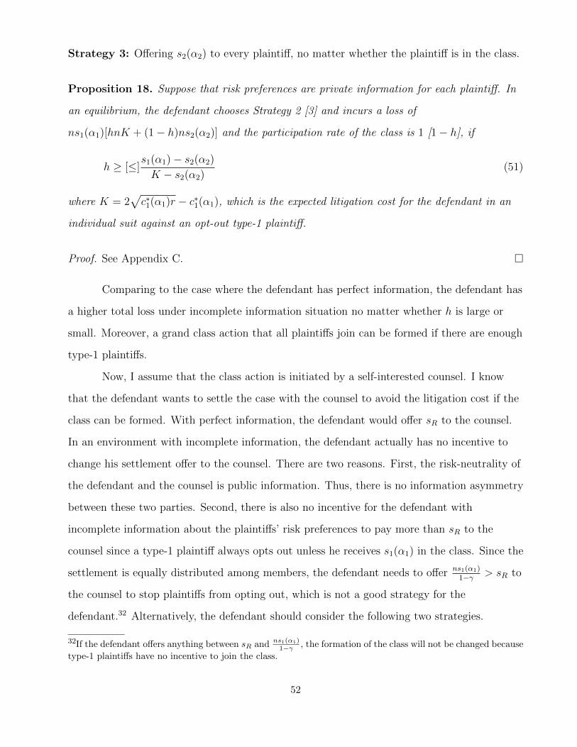
Strategy 3: Offering s2(α2) to every plaintiff, no matter whether the plaintiff is in the class.

Proposition 18. Suppose that risk preferences are private information for each plaintiff. In

an equilibrium, the defendant chooses Strategy 2 [3] and incurs a loss of

ns1(α1)[hnK + (1− h)ns2(α2)] and the participation rate of the class is 1 [1− h], if

h ≥ [≤]s1(α1)− s2(α2)

K − s2(α2)(51)

where K = 2√c∗1(α1)r − c∗1(α1), which is the expected litigation cost for the defendant in an

individual suit against an opt-out type-1 plaintiff.


Comparing to the case where the defendant has perfect information, the defendant has

a higher total loss under incomplete information situation no matter whether h is large or

small. Moreover, a grand class action that all plaintiffs join can be formed if there are enough

type-1 plaintiffs.

Now, I assume that the class action is initiated by a self-interested counsel. I know

that the defendant wants to settle the case with the counsel to avoid the litigation cost if the

class can be formed. With perfect information, the defendant would offer sR to the counsel.

In an environment with incomplete information, the defendant actually has no incentive to

change his settlement offer to the counsel. There are two reasons. First, the risk-neutrality of

the defendant and the counsel is public information. Thus, there is no information asymmetry

between these two parties. Second, there is also no incentive for the defendant with

incomplete information about the plaintiffs’ risk preferences to pay more than sR to the

counsel since a type-1 plaintiff always opts out unless he receives s1(α1) in the class. Since the

settlement is equally distributed among members, the defendant needs to offer ns1(α1)1−γ > sR to

the counsel to stop plaintiffs from opting out, which is not a good strategy for the

defendant.32 Alternatively, the defendant should consider the following two strategies.

32If the defendant offers anything between sR and ns1(α1)1−γ , the formation of the class will not be changed because

type-1 plaintiffs have no incentive to join the class.

52

Strategy 4: Offering sR to the counsel and offering s1(α1) to an opt-out plaintiff.

Strategy 5: Offering sR to the counsel and offering s2(α2) to an opt-out plaintiff.

The downside of Strategy 4 is type-2 plaintiffs would opt out and pretend to be type-1

plaintiffs to receive s1(α1). Consequently, the class will not be formed because no one wants

to join it. This strategy only works when h is large enough since the defendant does not want

to expend a large amount of resources at trial to fight against opt-out type-1 plaintiffs if he

offers s2(α2) to each opt-out plaintiff. Nevertheless, the cost of Strategy 5 for the defendant is

the litigation cost in individual suits against type-1 plaintiffs, while the benefit is to lower the

over-payment to type-2 plaintiffs. In this case, all type-2 plaintiffs join the class to receive

sp > s2(α2). The defendant still overpays them but it is less than s1(α1). The following

proposition summarizes the optimal decision of the defendant and the equilibrium with

incomplete information.

Proposition 19. Suppose that risk preferences are private information for each plaintiff, and

a class action is initiated by a self-interested counsel. In an equilibrium, the defendant chooses

Strategy 4 [5] and incurs a loss of ns1(α1) [hnK + sR] and the participation rate of the class is

0 [1− h], if

h ≥ [≤]ns1(α1)− sR

nK(52)

where K = 2√c∗1(α1)r − c∗1(α1).


The financial cost of allowing a self-interested counsel to initiate a class action is the

contingent fee. The contingent fee gives incentive to the counsel to fight against the defendant

and can increase the defendant’s total payment. Type-2 plaintiffs may also be better off by

joining the class with a counsel. Thus, this is not a bad cost if the goal is to punish the

defendant. However, the class initiated by a counsel may not be able to form if there are

enough type-1 plaintiffs. In this situation, the defendant has an incentive to break down the

class by offering high settlement to opt-out plaintiffs. Nevertheless, a grand class can be

53

formed if the defendant wants to offer every plaintiff the higher settlement in the case where

the class action is initiated by plaintiffs.

Next, I consider a situation where both types of plaintiffs want to join the class action

with a counsel. Suppose that there are two types of plaintiffs. One type has α3 and the other

has α4. Both s3(α3) and s4(α4) are less than sp. Without loss of generality, I assume that

α3 < α4, which implies that type-4 plaintiffs are more risk-averse than type-3 plaintiffs.

According to our results in Section 2, both type-3 and type-4 plaintiffs are risk-averse enough

to not have strong incentives to sue the defendant individually. In an environment without a

self-interested counsel, the formation of the class is the same as the one described in

Proposition 18. Compared to Proposition 18, the only difference in the current situation is

that the defendant incurs a smaller loss.

If a self-interested counsel is allowed to initiate the class action and charge a

contingent fee on the settlement, both types of plaintiffs join the class because they can

receive higher payments. Thus, a grand class is formed. In this case, the only party who gets

worse off is the defendant, because he has to pay more for each plaintiff. It is straightforward

to generalize this result into a situation where there are more than two types of plaintiffs but

they are all risk-averse enough to have more disadvantages in individual suits. Therefore, a

grand class which can benefit all plaintiffs can be formed even though the counsel who

initiates it is self-interested. The above argument is summarized in the following proposition.

Proposition 20. Suppose that risk preferences are private information for each plaintiff, and

a class action is initiated by a self-interested counsel. If all plaintiffs are risk-averse enough

such that si(αi) < sp for i = 1, ..., n, it is beneficial for them to join the class. The

participation rate of the class is 1.

5. Conclusion and Discussion

This paper examines the effects of risk aversion in the formation of a class action suit.

Risk aversion discourages plaintiffs to sue the defendant individually to some extent. Plaintiffs

with high degrees of risk aversion are likely to join a class action and can be better off in a

54

class action initiated by a risk-neutral counsel. Baik and Kim (1997) find that a player would

like to hire a delegate with more ability to compete for a prize on behalf of the player in a

contest. In this model, I consider litigation as a contest between disputing parties. I find that

a plaintiff’s legal investment and the probability of winning at trial are decreasing in the

degree of risk aversion in an individual suit. Thus, a risk-neutral counsel can be considered as

a delegate with more ability in this legal contest if plaintiffs are risk-averse enough.

In a class action, the main risk in litigation is transferred from plaintiffs to the

risk-neutral counsel. Why do not all risk-averse plaintiffs join the class action? First, the

self-interested counsel spends efforts to only match the contingent fee instead of the total

compensation for plaintiffs in the class. I find that the self-interested counsel’s legal

investment is strictly increasing in γ, his share of the total payoff. It is straightforward to

show that the counsel’s probability of winning at trial is 0.5 if γ = 1. Since the counsel is

self-interested, the defendant is still favored in terms of probability of winning at trial when

γ < 1. Second, higher γ can induce the counsel to invest more and increase the probability of

winning at trial but also lower the payoff per class member if the class wins. Therefore, the

payoff risk in a class does not necessarily have first-order stochastic dominance over the payoff

risk in an individual suit. Moreover, the settlement depends on the expected payoff in

litigation. Thus, plaintiffs with low degrees of risk aversion can opt out to receive higher

settlement offers because their relatively high expected payoff in the case of litigation.

If all plaintiffs are risk-averse enough, they will all join the class action initiated by a

self-interested counsel. Eisenberg and Miller (2004) find empirical evidence that opt-outs from

class actions are rare. One plausible explanation is that most plaintiffs who are involved with

class actions have high degrees of risk aversion. Even though a self-interested counsel can be

preferred in some circumstances, self-interest may induce the counsel only to initiate class

actions with large stakes and ignore potential class actions with small stakes. A full discussion

of this issue is beyond the scope of this paper but warrants further studies.

55

REFERENCES

[1] Andreoni, J., 1988, Privately Provided Public Goods in a Large Economy: the Limits ofAltruism, Journal of Public Economics, 35: 57-73.

[2] Baik, K. H., and I. G. Kim, 1997, Delegation in Contests, European Journal of PoliticalEconomy, 13: 281-298.

[3] Baik, K. H. , Shogren, J. F., 1992, Strategic Behavior in Contests: Comment, AmericanEconomic Review, 82: 359-362.

[4] Baye, M. R., Kovenock, D., de Vries, C. G., 1994, The Solution to the TullockRent-Seeking Game When R > 2: Mixed Strategy Equilibria and Mean Dissipation Rates,Public Choice, 81: 363-380.

[5] Baye, M. R., Kovenock, D., de Vries, C. G., 1999, The Incidence of Overdissipation inRent-Seeking Contests, Public Choice, 99: 439-454.

[6] Bergstrom, T., L. Blume, and H. Varian, 1986, On the Private Provision of Public Goods,Journal of Public Economics, 29: 25-49.

[7] Baye, M. R., Shin, O., 1999, Strategic Behavior in Contests: Comment, AmericanEconomic Review, 89: 691-693.

[8] Bellemare, C., Shearer, B., 2010, Sorting, Incentives, and Risk Preferences: Evidence froma Field Experiment, Economics Letters, 108: 345-348.

[9] Berg, J., Dickhaut, J., McCabe, K., 2005, Risk Preference Instability across Institutions:A Dilemma, Proceedings of the National Academy of Sciences, 102: 4209-4214.

[10] Bos, O., 2011, How Lotteries Outperform Auctions, Economics Letters, 110: 262-264.

[11] Bos, O., 2016, Charity Auctions for the Happy Few, Mathematical Social Sciences, 79:83-92.

[12] Carpenter, J. and P. H. Matthews, 2017, Using Raffles to Fund Public Good: Lessonsfrom a Field Experiment, Journal of Public Economics, 150: 30-38.

[13] Che, Y. K., 1996, Equilibrium Formation of Class Action Suits, Journal of PublicEconomics, 62: 339-361.

[14] Che, Y. K., 2002, The Economics of Collective Negotiation in Pretrial Bargaining,International Economic Review, 43: 549-575.

56

[15] Corazzini, L., M. Faravelli, and L. Stanca, 2010, A Prize to Give for: An Experiment onPublic Good Funding Mechanisms, Economic Journal, 120: 944-967.

[16] Cornes, R., and R. Hartley, 2003, Risk Aversion, Heterogeneity and Contests, PublicChoice, 117: 1-25.

[17] Cornes, R., and R. Hartley, 2005, Asymmetric Contests with General Technologies,Economic Theory, 26: 923-946.

[18] Cornes, R., Hartley, R., 2012, Risk Aversion in Symmetric and Asymmetric Contests,Economic Theory, 51: 247-275.

[19] Crainich, D., Eeckhoudt, L., 2008, On the Intensity of Downside Risk Aversion, Journalof Risk and Uncertainty, 36: 267-276.

[20] Dale, D., 2004, Charitable Lottery Structure and Fund Raising: Theory and Evidence,Experimental Economics, 7: 217-234.

[21] Damianov, D. S. and R. Peeters, 2018, Prize-Based Mechanisms for Fund-Raising:Theory and Experiments, Economic Inquiry, 56: 1562-1584.

[22] Deffains, B., and E. Langlais, 2011, Informational Externalities and Settlements in MassTort Litigations, European Journal of Law and Economics, 32: 241-262.

[23] Dixit, A., 1987, Strategic Behavior in Contests, American Economic Review, 77: 891-898.

[24] Duncan, B., 2002, Pumpkin Pies and Public Goods: The Raffle Fundraising Strategy,Public Choice, 111: 49-71.

[25] Eckel, C. C., El-Gamal, M. A., Wilson, R. K., 2009, Risk Loving after the Storm: ABayesian-Network Study of Hurricane Katrina Evacuees, Journal of Economic Behavior &Organization, 69: 110-124.

[26] Eeckhoudt, L., Gollier, C., 2005, The Impact of Prudence on Optimal Prevention,Economic Theory, 26: 989-994.

[27] Ehrlich, I., Becker, G., 1972, Market Insurance, Self-Insurance, and Self-Protection,Journal of Political Economy, 80: 623-648.

[28] Eisenberg, T., and G. Miller, 2004, The Role of Opt-Outs and Objectors in Class ActionLitigation: Theoretical and Empirical Issues, Vanderbilt Law Review, 57: 1529-1567.

[29] Emons, W., 2006, Playing it Safe with Low Conditional Fees versus Being Insured byHigh Contingent Fees, American Law and Economics Review, 8: 20-32.

[30] Emons, W., 2007, Conditional versus Contingent Fees, Oxford Economic Papers, 59:89-101.

57

[31] Farmer, A., and P. Pecorino, 1999, Legal Expenditure as a Rent-Seeking Game, PublicChoice, 100: 271-288.

[32] Faravelli, M. and L. Stancab, 2012, When Less is More: Rationing and Rent Dissipationin Stochastic Contests, Games and Economic Behavior, 74: 170-183.

[33] Faravelli, M. and L. Stancab, 2014, Economic Incentives and Social Preferences: CausalEvidence of Non-separability, Journal of Economic Behavior & Organization, 108:273-289.

[34] Fonseca, M. A., 2009, An Experimental Investigation of Asymmetric Contests,International Journal of Industrial Organization, 27: 582-591.

[35] Franke, J. and W. Leininger, 2014, On the Efficient Provision of Public Goods by Meansof Biased Lotteries: The Two Player Case, Economics Letters, 125: 436-439.

[36] Gneezy, U., Smorodinsky, R., 2006, All-Pay Auctions-An Experimental Study, Journal ofEconomic Behavior & Organization, 61: 255-275.

[37] Goerg, S., J. Lightle, and D. Ryvkin, 2016, Priming the Charitable Pump: AnExperimental Investigation of Two-Stage Raffles, Economic Inquiry, 54: 508-519.

[38] Goeree, J. K., E. Maasland, S. Onderstal, and J. L. Turner, 2005, How (Not) to RaiseMoney, Journal of Political Economy, 113: 897-918.

[39] Houser, D., Stratmann, T., 2012, Gordon Tullock and Experimental Economics, PublicChoice, 152: 211-222.

[40] Isaac, R. M., James, D., 2000, Just Who Are You Calling Risk Averse?, Journal of Riskand Uncertainty, 20: 177-187.

[41] Jensen, M. K., 2016, Existence, Uniqueness, and Comparative Statics in Contests, In:von Mouche, P., Quartieri, F. (Eds.), Equilibrium Theory for Cournot Oligopolies andRelated Games, Springer International Publishing, Switzerland, pp. 233-244.

[42] Jindapon, P., Neilson, W. S., 2007, Higher-Order Generalizations of Arrow-Pratt andRoss Risk Aversion: A Comparative Statics Approach, Journal of Economic Theory, 136:719-728.

[43] Jindapon, P., Whaley, C. A., 2015, Risk Lovers and the Rent Over-Investment Puzzle,Public Choice, 164: 87-101.

[44] Klement, A., and Z. Neeman, 2004, Incentive Structures for Class Action Lawyers,Journal of Law, Economics, & Organization, 20: 102-124.

[45] Kolmar, M. and D. Sisak, 2014, (In)efficient Public-Goods Provision Through Contests,Social Choice and Welfare, 43: 239-259.

58

[46] Kolmar, M. and A. Wagener, 2012, Contests and the Private Production of PublicGoods, Southern Economic Review, 79: 161-179.

[47] Landry, C. E., A. Lange, J. A. List, M. K. Price, and N. G. Rupp, 2006, Toward anUnderstanding of the Economics of Charity: Evidence from a Field Experiment,Quarterly Journal of Economics, 121: 747-782.

[48] Lange, A., J. A. List, and M. K. Price, 2007a, A Fundraising Mechanism Inspired byHistorical Tontines: Theory and Experimental Evidence, Journal of Public Economics,91: 1750-1782.

[49] Lange, A., J. A. List, and M. K. Price, 2007b, Using Lotteries to Finance Public Goods:Theory and Experimental Evidence, International Economic Review, 48: 901-927.

[50] Lim, W., Matros, A., Turocy, T. L., 2014, Bounded Rationality and Group Size inTullock Contests: Experimental Evidence, Journal of Economic Behavior & Organization,99: 155-167.

[51] Lynk, W., 1990, The Courts and the Market: An Economic Analysis of Contingent Feesin Class-Action Litigation, Journal of Legal Studies, 19: 247-260.

[52] Lynk, W., 1994, The Courts and the Plaintiffs’ Bar: Awarding the Attorney’s Fee inClass-Action Litigation, Journal of Legal Studies, 23: 185-209.

[53] Maeda, A., 2008, Optimal Lottery Design for Public Financing, Economic Journal, 118:1698-1718.

[54] Marceau, N., and S. Mongrain, 2003, Damage Averaging and the Formation of ClassAction Suits, International Review of Law and Economics, 23: 63-74.

[55] Morgan, J., 2000, Financing Public Goods by Means of Lotteries, Review of EconomicStudies, 67: 761-784.

[56] Morgan, J. and M. Sefton, 2000, Funding Public Goods with Lotteries: ExperimentalEvidence, Review of Economic Studies, 67: 785-810.

[57] Morgan, J., 2003, Sequential Contests, Public Choice, 116: 1-18.

[58] Morgan, J., Vardy, F., 2007, The Value of Commitment in Contests and TournamentsWhen Observation Is Costly, Games and Economic Behavior, 60: 326-338.

[59] Olson, M., 1965, The Logic of Collective Action. Cambridge, MA: Havard UniversityPress.

[60] Pecorino, P., 2015, Olson’s Logic of Collective Action at Fifty, Public Choice, 162:243-262.

59

[61] Pecorino, P. and A. Temimi, 2007, Lotteries, Group Size, and Public Good Provision,Journal of Public Economic Theory, 9: 451-466.

[62] Pecorino, P. and A. Temimi, 2012, Lotteries, Public Good Provision and the Degree ofRivalry, International Tax and Public Finance, 19: 195-202.

[63] Platt, B. C., Price, J., Tappen, H., 2013, The Role of Risk Preferences in Pay-to-BidAuctions, Management Science, 59: 2117-2134.

[64] Rosenberg, D., and K. Spier, 2014, Incentives to Invest in Litigation and the Superiorityof the Class Action, Journal of Legal Analysis, 6: 305-365.

[65] Sacconi, L., 2011, The Case against Lawyers’ Contingent Fees and the Misapplication ofPrincipal-Agent Models, European Journal of Law and Economics, 32: 263-292.

[66] Sandler, T., 2015, Collective Action: Fifty Years Later Public Choice, 164: 195-216.

[67] Sheremeta, R. M., 2010, Experimental Comparison of Multi-Stage and One-StageContests, Games and Economic Behavior, 68: 731-747.

[68] Sheremeta, R. M., 2011, Contest Design: An Experimental Investigation, EconomicInquiry, 49: 573-590.

[69] Sheremeta, R. M., 2013, Overbidding and Heterogeneous Behavior in ContestExperiments, Journal of Economic Surveys, 27: 491-514.

[70] Szidarovszky, F., Okuguchi, K., 1997, On the Existence and Uniqueness of Pure NashEquilibrium in Rent-Seeking Games, Games and Economic Behavior, 18: 135-140.

[71] Treich, N., 2010, Risk-Aversion and Prudence in Rent-Seeking Games, Public Choice,145: 339-349.

[72] Tullock., G., 1980, Efficient Rent Seeking. In: Buchanan, J. M., R.D. Tollison, and G.Tullock (Eds.), Toward a Theory of the Rent-Seeking Society. Texas A&M UniversityPress, College Station, TX, pp. 97-112.

[73] Warr, P. G., 1982, Pareto Optimal Redistribution and Private Charity, Journal of PublicEconomics, 19: 131-138.

60

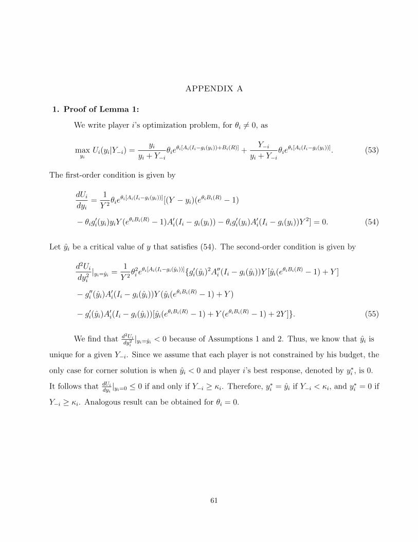
APPENDIX A

1. Proof of Lemma 1:

We write player i’s optimization problem, for θi 6= 0, as

maxyi

Ui(yi|Y−i) =yi

yi + Y−iθie

θi[Ai(Ii−gi(yi))+Bi(R)] +Y−i

yi + Y−iθie

θi[Ai(Ii−gi(yi))]. (53)

The first-order condition is given by

dUidyi

=1

Y 2θie

θi[Ai(Ii−gi(yi))][(Y − yi)(eθiBi(R) − 1)

− θig′i(yi)yiY (eθiBi(R) − 1)A′i(Ii − gi(yi))− θig′i(yi)A′i(Ii − gi(yi))Y 2] = 0. (54)

Let yi be a critical value of y that satisfies (54). The second-order condition is given by

d2Uidy2

i

|yi=yi =1

Y 2θ2i eθi[Ai(Ii−gi(yi))]{g′i(yi)2A′′i (Ii − gi(yi))Y [yi(e

θiBi(R) − 1) + Y ]

− g′′i (yi)A′i(Ii − gi(yi))Y (yi(e

θiBi(R) − 1) + Y )

− g′i(yi)A′i(Ii − gi(yi))[yi(eθiBi(R) − 1) + Y (eθiBi(R) − 1) + 2Y ]}. (55)

We find that d2Uidy2i|yi=yi < 0 because of Assumptions 1 and 2. Thus, we know that yi is

unique for a given Y−i. Since we assume that each player is not constrained by his budget, the

only case for corner solution is when yi < 0 and player i’s best response, denoted by y∗i , is 0.

It follows that dUidyi|yi=0 ≤ 0 if and only if Y−i ≥ κi. Therefore, y∗i = yi if Y−i < κi, and y∗i = 0 if

Y−i ≥ κi. Analogous result can be obtained for θi = 0.

61


Given the definition of share function si(Y ) :=y∗i

(y∗i +Y−i)and the first-order condition in

(54), we find that, if Y−i < κi and given θi 6= 0, player i chooses y∗i such that si(Y ) satisfies

(1− si(Y ))(eθiBi(R) − 1)

(si(Y )(eθiBi(R) − 1) + 1)θiA′i(Ii − gi(si(Y )Y ))− g′i(si(Y )Y )Y = 0. (56)

Define λ(si) as the left-hand side of (56). We find that λ(1) < 0 and λ(0) > 0 whenever

Y < κi. Since λ′(si) < 0, there exists a unique value of si > 0 such that (56) holds if Y < κi.

If Y−i ≥ κi, player i chooses y∗i = 0. It follows that Y = Y−i and hence si(Y ) = 0 if Y ≥ κi.

When θi = 0, the optimization problem is much simpler. Following similar arguments,

we find that player i chooses y∗i such that si(Y ) satisfies

(1− si(Y ))Ci(R)− g′i(si(Y )Y )Y = 0 (57)

if Y < Ci(R)g′i(0)

, otherwise si(Y ) = 0.

Property 1: Given Y ∈ (0, κi) and the definition of κi in (6), player i’s share, si,

implicitly defined by (56) can be written as

g′i(siY )Y

g′i(0)κi· A′i(Ii − gi(siY ))

A′i(Ii)=

1− si1− si + sieθiBi(R)

(58)

and it is continuous in Y .

Property 2: An increase in Y will cause the left-hand side of (58) to rise because gi is

convex and Ai is concave. To keep both sides equal, si must fall. A decrease in si will lower

the left-hand side and also increase the right-hand side of (58).

Property 3: As Y → 0, the left-hand side of (58) approaches zero. To maintain the

equality, the right-hand side must converge to zero and therefore si → 1. As Y → κi, the

left-hand side of (58) approachesg′i(siκi)

g′i(0)· A′i(Ii−gi(siκi))

A′i(Ii)which is greater than or equal to 1

because gi is convex and Ai is concave. Since the right-hand side never exceeds 1, to maintain

the equality, both sides must converge to 1 and therefore si → 0.

62

3. Proof of Proposition 2:

Given the generalized CARA utility function, we can write

κi =

eθiαiR−1θiαig′i(0)

if θi 6= 0

Rg′i(0)

if θi = 0.

(59)

Part 1: If f ′i(0) =∞, then g′i(0) = 0 and κi =∞. Since si(Y ) > 0 for all Y > 0, then

si(Ye) > 0 and xei > 0.

Part 2: Property: κi is strictly increasing in θiαi.

dκidθiαi

=

θiαiRe

θiαiR−eθiαiR+1(θiαi)2g′i(0)

if θi 6= 0

R2

2g′i(0)if θi = 0.

(60)

Thus, to prove dκidθiαi

> 0, we only have to show that θiαiReθiαiR − eθiαiR + 1 > 0 given any

θi 6= 0. Define H(z) = ez − z. We have H ′(z) = ez − 1 and H ′′(z) = ez. We find that H(z) is a

strictly convex function with the minimum value of 1 at z = 0. So ez − z > 1 for all z 6= 0.

Letting z = −θiαiR where θi 6= 0 yields e−θiαiR + θiαiR > 1. By multiplying both sides of this

inequality by eθiαiR, we have 1 + θiαiReθiαiR > eθiαiR, that is, θiαiRe

θiαiR − eθiαiR + 1 > 0

given any θi 6= 0. Given identical production functions and θ1α1 ≤ ... ≤ θnαn, we know that

κ1 ≤ ... ≤ κn. If xek = 0, then sk(Ye) = 0 and we know from Lemma 2 that Y e ≥ κk. It follows

that Y e ≥ κi and hence xei = 0 for all i = 1, ..., k − 1.


Part 1: In the proof of Proposition 2 part 2, we find that H(z) = ez − z > 1 for all

z 6= 0. Letting z = θiαiR yields eθiαiR − 1 > θiαiR whenever θi 6= 0. We obtain the result in

part 1 by dividing both sides by θiαi.

Part 2: Given (10), we find ∂2si(Y )∂Y 2 = 2κie

θiαiR(eθiαiR−1)

(κi−Y+Y eθiαiR)3. Since the denominator is positive for

all Y < κi, the sign of ∂2si(Y )∂Y 2 is the same as the sign of (eθiαiR − 1).

63


Part 1: Consider (9) and (12). For the inequality in (12) to hold, κ must be greater

than R. According to Proposition 3, we need θ > 0. Thus rent over-dissipation will not occur

in equilibrium when θ ≤ 0. Solving for n from (12) given κ > R and the definition of κ in (9)

yields n > 1 + J(z) where J(z) = zez

ez−z−1and z = αR.

Part 2: Given z > 0, J(z) is a strictly convex function with the minimum value of 3.35

at z = 1.79. If n ≤ 4, then we have n < 1 + J(αR) for any α > 0, and rent over-dissipation

will not occur in equilibrium.


We define ψ as Y such that s1(Y ) = s2(Y ). Thus, ψ is where the two share functions

cross. Knowing ψ will help us determine the favorite and underdog in equilibrium based on θi

and αi for i = 1, 2.

Case 1: |θ1α1| = |θ2α2|. If θ1α1 = θ2α2, then it follows immediately that xe1 = xe2.

Suppose that θ1α1 = −θ2α2. Let Yi be Y ∈ (0, κi) such that si(Y ) = 12

for i = 1, 2. Given (9)

and (10), we find Yi = eθiαiR−1θiαi(eθiαiR+1)

when θi 6= 0. Given θ1 = −θ2 and α1 = α2, we have

Y1 =e−θ2α2R − 1

−θ2α2(e−θ2α2R + 1)=

1− eθ2α2R

−θ2α2(1 + eθ2α2R)=

eθ2α2R − 1

θ2α2(eθ2α2R + 1)= Y2. (61)

Thus, ψ = Y1 = Y2 and s1(ψ) = s2(ψ) = 12. It follows that xe1 = xe2 = ψ

2.

Case 2: |θ1α1| < |θ2α2|. Properties of each player’s share function derived in

Proposition 3 suggest that

(1) if θ2 = −1, then s1(ψ) = s2(ψ) > 12

and s1(Y ) ≶ s2(Y ) given Y ≶ ψ; and

(2) if θ2 = 1, then s1(ψ) = s2(ψ) < 12

and s1(Y ) ≷ s2(Y ) given Y ≶ ψ.

If player 2 is risk-averse, then we know from (9) that κ1 > κ2. Since s1(ψ) = s2(ψ) > 12

and both s1(Y ) and s2(Y ) are strictly decreasing, we find that Y e > ψ. Since s1(Y ) > s2(Y )

for any Y ∈ (ψ, κ2), then s1(Y e) > s2(Y e) and xe1 > xe2.

64

If player 2 is risk-loving, then we know from (9) that κ1 < κ2. Since s1(ψ) = s2(ψ) < 12

and both s1(Y ) and s2(Y ) are strictly decreasing, we find that Y e < ψ. Since s1(Y ) > s2(Y )

given Y ∈ (0, ψ), then s1(Y e) > s2(Y e) and xe1 > xe2.

Therefore, |θ1α1| ≶ |θ2α2| implies xe1 ≷ xe2.


Player 1’s second-order condition is satisfied if

dΦ1(x1)

dx1

= θ31α

21[p(x1)eθ1α1(I1+R−x1) + (1− p(x1))eθ1α1(I1−x1)]

− 2θ21α1[eθ1α1(I1+R−x1) − eθ1α1(I1−x1)]p′(x1) + θ1[eθ1α1(I1+R−x1) − eθ1α1(I1−x1)]p′′(x1)

= −θ1α1Φ1(x1) + θ1[eθ1α1(I1+R−x1) − eθ1α1(I1−x1)][p′′(x1)− θ1α1p′(x1)] (62)

is negative. Since Φ1(x1) = 0 and θ1[eθ1α1(I1+R−x1) − eθ1α1(I1−x1)] > 0, it follows from (62) that

player 1’s second-order condition is satisfied if p′′(x1)− θ1α1p′(x1) < 0. If θ1 = 0, the

second-order condition is satisfied if p′′(x1) < 0.

Given x∗2(x1) in (16), we rewrite

p(x1) =A

θ2α2 +√

(θ2α2)2 + 2Ax1

(63)

where A := 2θ2α2eθ2α2R

eθ2α2R−1= 2eθ2α2R

κ2> 0 for all θ2α2. We find that

p′(x1) =A2

x21

√(θ2α2)2 + 2A

x1

(θ2α2 +

√(θ2α2)2 + 2A

x1

)2 > 0. (64)

Let B := (θ2α2)2 + 2Ax1> 0. The denominator in (64) can be written as C2, where

C := θ2α2x1B14 + x1B

34 > 0. Thus, we have

p′′(x1) = −2A2

C3

dC

dx1

. (65)

65

We find that

dC

dx1

= (θ2α2 +B12 )B

14 − A(θ2α2 + 3B

12 )

2B34x1

. (66)

Thus dCdx1

> 0 if and only if

D :=(θ2α2 +

√B)Bx1

(θ2α2 + 3√B)

− eθ2α2R

κ2

> 0. (67)

If θ2α2 ≥ 0, then (67) always holds. If θ2α2 < 0, to show that (67) holds we need to restrict

the possible values of x1 to be in the interval (0, κ2), the set of all possible interior solutions

for player 1. Note that player 1 will not choose x1 > κ2 because x1 = κ2 is large enough to

drive player 2 out from the contest. We find that (i) ∂D∂R

< 0 and (ii) limR→∞

D = 0 because

limR→∞

A = 0 for all θ2α2 < 0. These two properties of D imply that D > 0 for all θ2α2 < 0.

Thus we can conclude that dCdx1

> 0 and p′′(x1) < 0 for all θ2α2. It follows that the

second-order condition for player 1 always holds as long as θ1α1 > ρ where ρ = p′′(x1)p′(x1)

< 0.


First, we try to find whether the slope of player 2’s best response function evaluated at

the Nash equilibrium in simultaneous contest, i.e.,dx∗2dx1|x1=xe1

, is positive or negative. Since

dx∗2dx1

= −∂Φ2/∂x1∂Φ2/∂x2

, the slope of player 2’s best-response function and ∂Φ2

∂x1have the same sign.

Given Φ2(x1, x2) in (14), we have

∂Φ2

∂x1

=

[θ2(eθ2α2(I2+R−x2) − eθ2α2(I2−x2))

(x1 + x2)3

][θ2α2x2(x1 + x2) + (x2 − x1)]. (68)

Since the first bracketed term is positive, the sign of the right-hand side of (68) depends on

the second bracketed term. That is,dx∗2dx1|x1=xe1

≷ 0 whenever θ2α2xe2(xe1 + xe2) + (xe2 − xe1) ≷ 0.

We know from Proposition 5 that |θ1α1| ≶ |θ2α2| implies xe1 ≷ xe2. Therefore, if |θ1α1| ≶ |θ2α2|

and θ2 ≶ 0, then θ2α2xe2(xe1 + xe2) + (xe2 − xe1) ≶ 0 and

dx∗2dx1|x1=xe1

≶ 0. It follows that

(1) if |θ1α1| ≤ |θ2α2| and θ2 = −1, then xs1 > xe1 ≥ xe2 > xs2.

(2) if |θ1α1| ≥ |θ2α2| and θ2 = 1, then xs1 < xe1 and xs2 < xe2. Since xe2 ≥ xe1, we know that

(xe1, xe2) is on or above the 45-degree line. The properties of player 2’s best response

66

derived in Footnote 12 implies that, in the first stage of a sequential contest, player 1

finds her optimal investment by moving along player 2’s best-response curve to the left

of (xe1, xe2). It follows that (xs1, x

s2) is strictly above the 45-degree line. Therefore,

xs1 < xs2.


Given θ1 = 0, player 1’s first-order condition in (18) suggests that the corner solution

where xs1 = κ2 will be obtained if

−1 +Rp′(κ2) ≥ 0. (69)

This condition is equivalent to

e2θ2α2R − θ2α2R− 1 ≥ 0 (70)

Define K(z) = e2z − z − 1. We have K ′(z) = 2e2z − 1 and K ′′(z) = 4e2z > 0. We find that

K(z) ≥ 0 when z ≤ −45. Letting z = θ2α2R yields e2θ2α2R − θ2α2R− 1 ≥ 0 whenever

θ2α2R ≤ −45.

67

APPENDIX B


Parts 1 and 2 follow from the definition of si(X). Given κi > R, we find that

dsi(X)

dX=−e−αiR[αi − h′i(G)− h′′i (G)X]

(1− e−αiR){1− [αi − h′i(G)]X}2(71)

which is strictly negative for all X ∈ (R, κi).


Part 1: Given κi in (30), we have

∂κi∂αi

=(αi − βi)Re−αiR − 1 + e−αiR

(αi − βi)2. (72)

Define g(αi) := (αi − βi)Re−αiR − 1 + e−αiR. which is the numerator on the right-hand side of

(72). We find that g′(αi) = −(αi − βi)R2e−αiR < 0. In addition, we know that

g(0) = −βiR < 0. Therefore, g(αi) < 0 for all αi > 0.

Part 2: Given κi in (30), we have

∂κi∂βi

=1− e−αiR

(αi − βi)2> 0 (73)

for all αi > 0.


We find that

∂si∂αi

=e−αiRX{(αi − βi)R[1− (αi − βi)X]− (1− e−αiR)}

(1− e−αiR)2[1− (αi − βi)X]2. (74)

It follows that ∂si∂αiQ 0 if and only if X R Xi := R−κi

(αi−βi)R . If κi ≥ R, Xi ≤ 0. Since

X > 0, ∂si∂αi

< 0 if κi ≥ R. If κi < R, we find that si(Xi) >12, for all R > 0, which implies that

68

the intersection between any two share functions is above s = 12. Thus, total lottery purchases

in equilibrium (Xe) must be on the right of all intersections between share functions, i.e.

Xe > Xi, for i = 1, ..., n. Therefore, we know that ∂si∂αi≤ 0 in equilibrium and so

∂xei∂αi≤ 0, since

xei = si(Xe)Xe.

In addition, we find that

∂si∂βi

=(1− e−αiR)Xe−αiR

[1− e−αiR + (e−αiR − 1)(αi − βi)X]2> 0. (75)

Since ∂si∂βi

> 0 and ∂κi∂βi

> 0, we know that∂xei∂βi≥ 0.


Given αi = α, βi = β, and player i’s share function in (29),∑ni=1 si(R) = n(κ−R)

κ−(1−e−αR)R> 1 is equivalent to n > 1 + Re−αR

κ−R = 1 + (α−β)Re−αR

1−e−αR−(α−β)R.

Part 1: Given Ge(n,R) = Xe(n,R)−R and Xe(n,R) in (33), we have

∂Ge

∂n=∂Xe

∂n=

(1− e−αR)(α− β)(n+ 2e−αR − 2)

(n− 1 + e−αR)(α− β)> 0. (76)

Part 2: Given Xe(n,R) in (33), we have

limn→∞

Xe = limn→∞

κ(n− 1)

e−αR + n− 1= κ. (77)

Thus, limn→∞

Ge = κ−R > 0 since all players are relevant.


Given Xe in (33), we have

∂Xe

∂R=

(n− 1)nαe−αR

(α− β)(n− 1 + e−αR)2> 0 (78)

and ∂2Xe

∂R2 < 0 and limR→∞

∂Xe

∂R= 0. Hence, we know that there exists R such that Xe > R, i.e.

Ge > 0, for all R ∈ (0, R), if limR→0

∂Xe

∂R> 1, which implies β > α

n.

69


Public good provision is maximized when ∂Xe

∂R= 1, given (78), which implies that

(α− β)e−2αR + [2(α− β)− αn](n− 1)e−αR + (α− β)(n− 1)2 = 0. (79)

According to the proof of Proposition 13, we know that there is a unique solution for R to

maximize Ge. Thus, we find that R∗ will satisfy the following equality.

e−αR∗

=(n− 1)[(n− 2)α + 2β]− (n− 1)

√αn[(n− 4)α + 4β]

2(α − β). (80)

Part 1: Given (36), we have

∂R∗

∂n=

1

α

−N(n− 1)[(n− 2)α + 2β]− (n− 1)

√αn[(n− 4)α + 4β]

, (81)

where N =2[(2n−3)α+2β]

√αn[(n−4)α+4β]−[−4α2n2+2α(7α−6β)n−4α(α−β)]

2√αn[(n−4)α+4β]

. We find that N ≷ 0 if and

only if

32(2β − α)n− 16α ≷ 0. (82)

Therefore, ∂R∗

∂n> 0, because N < 0, if and only if β

α< 1

2+ 1

4n.

Part 2:

limn→∞

R∗(n) = limn→∞

1

α

{ln[2(α− β)]− ln

[2(n− 1)(α− β)2

(n− 2)α + 2β

]}(83)

=1

αln

(α

α− β

). (84)

Part 3: We find that

limn→∞

Xe(n,R∗(n)) = limn→∞

(1− e−αR∗(n))(1− 1n)

e−αR∗(n)

n+ 1− 1

n

=β

α(α− β). (85)

Therefore, we have

limn→∞

Ge(n,R∗(n)) = limn→∞

(Xe(n,R∗(n))−R∗(n)) =1

α

[β

α− β− ln

(α

α− β

)]. (86)

70


First, we define total expected utility of all players as U and evaluate U at xe.

U =n∑i=1

Eu =n∑i=1

{ 1

n

[−e−(α(I−xe+R)+βG)

]+n− 1

n

[−e−(α(I−xe)+βG)

]}. (87)

The first-order condition is

∂U

∂R= (α− β)(n− 1 + e−αR)e−(α(I−xe)+βG)L(R) = 0, (88)

where L(R) = (α− β)2e−2αR + (n− 1)[(n− 3)αβ + 2β2]e−αR − (n− 1)2(α− β)β.

By setting L(R) = 0, we obtain R in (37).


∂R

∂n= − 1

α

Q√(n− 1)2αβ[(n2 − 6n− 3)αβ + 4nβ2 + 4α2]− (n− 1)[(n− 3)αβ + 2β2]

(89)

where

Q =(n− 1)αβ[4αβn2 − (20αβ − 12β2)n+ 8α2 − 4β2]

2√

(n− 1)2αβ[(n2 − 6n− 3)αβ + 4nβ2 + 4α2]− (2αβn− 4αβ + 2β2). (90)

We also find that Q < 0, which implies that ∂R∂n

> 0, if and only if α < βn.

Part 2: We evaluate L(R) at R∗.

L(R∗) =N2

4(α− β), (91)

where

N2 =(α− β)(n− 1)2[(n− 2)α + β]2 + (α− β)(n− 1)2αn[(n− 4)α + 4β]+

2(n− 1)2[(n− 3)αβ + 2β2][(n− 2)α + 2β]−

2(α− β)(n− 1)2[(n− 2)α + 2β]√αn[(n− 4)α + 4β]−

2(n− 1)2[(n− 3)αβ + 2β2]√αn[(n− 4)α + 4β]− 4(n− 1)2(α− β)2β. (92)

71

We find that N2 < 0 if and only if βα> 1

n. Thus, L(R∗) < 0, given β

α> 1

n. Since

dL(R)dR

< 0, L(R∗) < 0 implies that R∗ > R.

Part 3:

limn→∞

R(n) = limn→∞

1

α

{ln[2(α− β)2]− ln

[2(n− 1)(α− β)3

(n− 3)α + 2β

]}(93)

=1

αln

(α

α− β

)= lim

n→∞R∗(n). (94)

8. Extension of the Functional Form of Utility Function

Suppose that hi(G) = βiln(G+ 1) for all i and αi ≥ βi > 0. Note that

h′i(G) = βiG+1

< αi and so ∂ui(wi,G)∂wi

> ∂ui(wi,G)∂G

. Each player’s utility function can be written as

ui(wi, G) = − e−αiwi

(G+ 1)βi. (95)

Player i’s share function is

si(X) =

(1−e−αiR)(X−R+1)−X[αi(X−R)+(αi−βi)]

(1−e−αiR){(X−R+1)−X[αi(X−R)+(αi−βi)]}, if X ∈ (R, κi)

0 if X ∈ [κi,∞)

(96)

where

κi =1− e−αiR − αi + βi + αiR +

√(1− e−αiR − αi + βi + αiR)2 + 4αi(1−R)(1− e−αiR)

2αi.

(97)

In this paper, we only consider equilibria where a positive amount of the public good is

provided (Xe > R). We find that κi > R, i.e., player i is relevant when αi and βi satisfy (31)

which is the same as when we assume hi(G) = βiG even though κi derived in (30) and (97)

are different. Given homogeneous players, the threshold of the number of players to lead to an

equilibrium with Ge > 0 is also the same as the one when hi(G) = βiG. The comparative

statics results regarding each player’s measure of risk aversion, αi, still hold.

72

Proposition 21. Suppose that Assumption 3 holds and hi(G) = βiln(G+ 1) for all i, and

αi ≥ βi > 0.

(1) There exists a unique equilibrium with Ge > 0 whenever the number of relevant players

is large enough.

(2) Given heterogeneous players with αi = βi for i = 1, ..., n, there exists a unique

equilibrium with Ge > 0 for any n ≥ 2.

(3) Given homogeneous players with αi = α and βi = β for i = 1, ..., n, there exists a

unique equilibrium with Ge > 0 if and only if n > 1 + (α−β)Re−αR


(4) Player i’s participation threshold κi is strictly decreasing in αi. Players with a larger

αi are more likely to free ride in equilibrium.

(5) Given heterogeneous players with αi = βi for i = 1, ..., n, each player’s lottery purchase

in equilibrium, xei , is decreasing in αi.

Proof. Part 1: It is implied by Proposition 9.

Part 2: Given αi = βi for i = 1, ..., n, and (96), we find that si(R) = 1. Therefore,∑ni=1 si(R) = n and so Ge = Xe −R > 0.

Part 3: Given αi = α, βi = β for i = 1, ..., n, and (96), the necessary and sufficient

condition for Ge > 0 provided in Proposition 9 (∑n

i=1 si(R) > 1) is equivalent to

n > 1 + (α−β)Re−αR



∂κi∂αi

=(αiRe

−αiR − 1 + e−αiR)[1− e−αiR − αi + βi + αiR+ 2(1−R)αi +√D1]− βi(1− e−αiR − αi + βi + αiR+

√D1)

2α2i

√D1

(98)

where D1 = (1− e−αiR − αi + βi + αiR)2 + 4αi(1−R)(1− e−αiR). Define

f(x) = xe−x − 1 + e−x. We have f ′(x) = −xe−x < 0 and f(0) = −1 < 0. Thus, f(x) < 0, for

all x ≥ 0. Letting x = αiR yields αiRe−αiR − 1 + e−αiR < 0. In addition, κi > R implies that

1− e−αiR − αi + βi + αiR + 2(1−R)αi +√D1. Additionally, since κi > 0,

1− e−αiR − αi + βi + αiR +√D1 > 0. Thus, the numerator of (98) is negative and so is ∂κi

∂αi.

73


∂si∂αi

=X(X −R)e−αiR[−α2

iRX2 + (e−αiR − 1 + αiR + α2

iR2)X + (1−R)(e−αiR − 1 + αiR)]

(1− e−αiR)2[X −R + 1− αiX(X −R)]2.

(99)

We find that ∂si∂αiQ 0 if and only if X R Xω

i , where

Xωi =

e−αiR − 1 + αiR + α2iR

2 +√D2

2α2iR

(100)

where D2 = (e−αiR − 1 + αiR + α2iR

2)2 + 4α2iR(1−R)(e−αiR − 1 + αiR). In addition, we find

that si(Xωi ) > 1

2, which implies that the intersection between any two share functions is above

s = 12. Thus, the equilibrium total purchase (Xe) must be on the right of all intersections

between share functions. In other words, Xe > Xωi , for i = 1, ..., n. Therefore, in equilibrium,

∂si(Xe)

∂αi≤ 0 and thus

∂xei∂αi≤ 0, since xei = si(X

e)Xe.

�

74

APPENDIX C


Define cT = ci + cD. Equation (42) can be written as

−e−αi(Ii−ci)

c2T

[αicicT e−αir + cDe

−αir + αicDcT − cD] = 0 (101)

which is equivalent to

cDcT

(e−αir − 1) + αicT (cicTe−αir +

cDcT

) = 0. (102)

Define pi = cicT

. Thus, I have that 1− pi = cDcT

. By substituting pi and 1− pi in (102),

plaintiff i’s probability that prevails at trial can be written as a function of cT :

pi(cT ) =1− e−αir − αicT

(1− e−αir)(1− αicT ). (103)

Following Cornes and Hartley (2003 and 2005), I call pi(cT ) plaintiff i’s share function.

According to Lemma 2 and Proposition 3, pi(cT ) is strictly decreasing and concave in cT . I

find that pi(cT ) rotates clockwise around the following point

θi =αiR− 1 + e−αiR

α2iR

(104)

when αi increases. Therefore, the probability of winning in equilibrium p∗i is decreasing in αi

because the equilibrium condition is that the sum of both disputing parties’ shares equals one.

So does the total investment c∗T . Since c∗i = p∗i c∗T , c∗i is also decreasing in αi.


I find that

∂c∗R∂γ

=2nrγ(1 + γ)

(1 + γ)4> 0; and

∂c∗D∂γ

=nr(1− γ2)

(1 + γ)4> 0. (105)

75


I find that

limαi→0+

si = − limαi→0+

log(e−αirp∗i + 1− p∗i )αi

− limαi→0+

(p∗i )2r (106)

=r

2− r

4(L′Hopital′s rule) =

r

4; (107)

limαi→+∞

si = − 0

∞− 0 = 0, because lim

αi→+∞p∗i = 0. (108)


The cost of Strategy 2 is ns1(α1) while the expected cost of Strategy 3 is

hnK + (1− h)ns2(α2), where K = 2√c∗1(α1)r − c∗1(α1), which is the expected litigation cost

for the defendant in an individual suit against an opt-out type-1 plaintiff. The defendant

chooses Strategy 2 if

ns1(α1) ≤ hnK + (1− h)ns2(α2) (109)

which implies that

h ≥ s1(α1)− s2(α2)

K − s2(α2). (110)


The defendant pays ns1(α1) totally by choosing Strategy 4. However, the expected

cost of Strategy 5 is hnK + sR, where K = 2√c∗1(α1)r − c∗1(α1). Strategy 4 is optimal if

ns1(α1) ≤ hnK + sR (111)

which implies that

h ≥ ns1(α1)− sRnK

. (112)

76

three essays on risk attitudes and the theory of …

Documents