essays in economic theory: strategic communication and

Essays in Economic Theory: Strategic Communication and Information Design

Andrew Kosenko

Submitted in partial fulfillment of therequirements for the degree of

Doctor of Philosophyin the Graduate School of Arts and Sciences

COLUMBIA UNIVERSITY

2018

ABSTRACT

Essays in Economic Theory: Strategic Communication and Information Design

Andrew Kosenko

This dissertation consists of four essays in economic theory. All of them fall un-

der the umbrella of economics of information; we study various models of game-

theoretic interaction between players who are communicating with others, and

have (or are able to produce) information of some sort. There is a large emphasis

on the interplay of information, incentives and beliefs.

In the first chapter we study a model of communication and persuasion be-

tween a sender who is privately informed and has state independent preferences,

and a receiver who has preferences that depend on the unknown state. In a model

with two states of the world, over the interesting range of parameters, the equi-

libria can be pooling or separating, but a particular novel refinement forces the

pooling to be on the most informative information structure in interesting cases.

We also study two extensions - a model with more information structures as well

as a model where the state of the world is non-dichotomous, and show that analo-

gous results emerge.

In the second chapter, which is coauthored with Joseph E. Stiglitz and Jungy-

oll Yun, we study the Rothschild-Stiglitz model of competitive insurance markets

with endogenous information disclosure by both firms and consumers. We show

that an equilibrium always exists, (even without the single crossing property), and

characterize the unique equilibrium allocation. With two types of consumers the

outcome is particularly simple, consisting of a pooling allocation which maximizes

the well-being of the low risk individual (along the zero profit pooling line) plus

a supplemental (undisclosed and nonexclusive) contract that brings the high risk

individual to full insurance (at his own odds). We also show that this outcome is

extremely robust and Pareto efficient.

In the third chapter we study a game of strategic information design between a

sender, who chooses state-dependent information structures, a mediator who can

then garble the signals generated from these structures, and a receiver who takes

an action after observing the signal generated by the first two players. Among

the results is a novel (and complete, in a special case) characterization of the set

of posterior beliefs that are achievable given a fixed garbling. We characterize

a simple sufficient condition for the unique equilibrium to be uninformative, and

provide comparative statics with regard to the mediator’s preferences, the number

of mediators, and different informational arrangements.

In the fourth chapter we study a novel equilibrium refinement - belief-payoff

monotonicity. We introduce a definition, argue that it is reasonable since it captures

an attractive intuition, relate the refinement to others in the literature and study

some of the properties.

Contents

List of Figures iii

Acknowledgements vi

Dedication ix

1 Bayesian Persuasion with Private Information 1

1.1 Introduction . . . . . . . . . . . . . . . . . . . . . . . . . . . . . . . . . 1

1.2 Relationship to Existing Literature . . . . . . . . . . . . . . . . . . . . 6

1.3 Model . . . . . . . . . . . . . . . . . . . . . . . . . . . . . . . . . . . . . 8

1.4 A General Model: Non-dichotomous States. . . . . . . . . . . . . . . . 43

1.5 Concluding Remarks . . . . . . . . . . . . . . . . . . . . . . . . . . . . 52

2 Revisiting Rothschild-Stiglitz 62

2.1 The Model . . . . . . . . . . . . . . . . . . . . . . . . . . . . . . . . . . 66

2.2 Rothschild-Stiglitz with Secret Contracts . . . . . . . . . . . . . . . . . 69

2.3 Pareto Efficiency with Undisclosed Contracts . . . . . . . . . . . . . . 73

2.4 Definition of Market Equilibrium . . . . . . . . . . . . . . . . . . . . . 77

2.5 Equilibrium Allocations . . . . . . . . . . . . . . . . . . . . . . . . . . 83

i

2.6 Equilibrium . . . . . . . . . . . . . . . . . . . . . . . . . . . . . . . . . 84

2.7 Generality of the Result . . . . . . . . . . . . . . . . . . . . . . . . . . . 89

2.8 Extensions: Non-uniqueness of Equilibrium . . . . . . . . . . . . . . . 90

2.9 Extensions to Cases with Many Types . . . . . . . . . . . . . . . . . . 92

2.10 Previous Literature . . . . . . . . . . . . . . . . . . . . . . . . . . . . . 94

2.11 The No-disclosure Limited Information Price Equilibria . . . . . . . . 97


2.13 Appendices . . . . . . . . . . . . . . . . . . . . . . . . . . . . . . . . . 104

3 Mediated Persuasion: First Steps 115

3.1 Introduction . . . . . . . . . . . . . . . . . . . . . . . . . . . . . . . . . 115

3.2 Environment . . . . . . . . . . . . . . . . . . . . . . . . . . . . . . . . . 122

3.3 Binary Model . . . . . . . . . . . . . . . . . . . . . . . . . . . . . . . . 136


3.5 Auxiliary Results . . . . . . . . . . . . . . . . . . . . . . . . . . . . . . 161

4 Things Left Unsaid: The Belief-Payoff Monotonicity Refinement 166

4.1 Introduction . . . . . . . . . . . . . . . . . . . . . . . . . . . . . . . . . 166

4.2 Environment . . . . . . . . . . . . . . . . . . . . . . . . . . . . . . . . . 170

4.3 Relationship to Other Refinements . . . . . . . . . . . . . . . . . . . . 174


Bibliography 185

ii

List of Figures

1.1 Illustration with pooling on ΠL, and the deviation to ΠH. . . . . . . . . . 29

2.1 Breaking the RS separating equilibrium in the presence of undisclosed

contracts at high-risk odds. . . . . . . . . . . . . . . . . . . . . . . . . . . 68

2.2 Sustaining an equilibrium in the presence of a cream-skimming deviant

contract D in z. . . . . . . . . . . . . . . . . . . . . . . . . . . . . . . . . . . 71

2.3 Pareto-efficient allocations ((A∗, C∗), (A ′, C ′)) and the equilibrium allo-

cation (A∗, C∗). . . . . . . . . . . . . . . . . . . . . . . . . . . . . . . . . . 75

2.4 Equilibrium without single-crossing. . . . . . . . . . . . . . . . . . . . . . 91

2.5 Equilibrium (A, B, C) with three types, which cannot be broken by D

as individuals of higher-risk type supplement it by additional pooling

insurance (along the arrow) without being disclosed to the deviant firm.

P−L denotes the average probability of accident for the two highest risk

types, while Vi indicates an indifference curve for i-risk type (i = H, M, L). 93

2.6 Breaking No-Disclosure-Information Price Equilibrium Pe by a fixed-

quantity contract (α ′, β ′), where Pe > P ′ > P. . . . . . . . . . . . . . . . . 101

iii

2.7 Nash Equilibrium can be sustained against multiple deviant contracts

(A∗B, G) or (A∗B ′, G) offered at different prices as high-risk individu-

als also choose G (over A∗B) or as (A∗B ′, G) yields losses for the deviant

firm (while inducing self-selection). . . . . . . . . . . . . . . . . . . . . . . 112

3.1 Illustration of the Model. . . . . . . . . . . . . . . . . . . . . . . . . . . . . 124

3.2 Effect of Garbling on Beliefs in a Dichotomy. . . . . . . . . . . . . . . . . 125

3.3 An Example. . . . . . . . . . . . . . . . . . . . . . . . . . . . . . . . . . . . 131

3.4 Comparing the Feasible Sets of Posteriors. . . . . . . . . . . . . . . . . . . 141

3.5 Increasing Noise Shrinks the Set of Feasible Posteriors. . . . . . . . . . . 142

3.6 Tracing the Outer Limit of F(M, π): First Boundary. . . . . . . . . . . . . 144

3.7 Tracing the Outer Limit of F(M, π): Second Boundary. . . . . . . . . . . . 145

3.8 Tracing the Outer Limit of F(M, π): Third Boundary. . . . . . . . . . . . 146

3.9 Tracing the Outer Limit of F(M, π): Fourth Boundary. . . . . . . . . . . . 147

3.10 F(M, π): an Illustration. . . . . . . . . . . . . . . . . . . . . . . . . . . . . 148

3.11 Key Features of the Feasible Set. . . . . . . . . . . . . . . . . . . . . . . . . 149

3.12 Blackwell’s Order Implies Set Inclusion for Feasible Sets. . . . . . . . . . 153

3.13 Further Illustration of Set Inclusion. . . . . . . . . . . . . . . . . . . . . . 154

3.14 Unranked Feasible Sets. . . . . . . . . . . . . . . . . . . . . . . . . . . . . 155

3.15 Going Beyond the Dichotomy: Three Signals. . . . . . . . . . . . . . . . 156

3.16 A Simple Non-trivial Example. . . . . . . . . . . . . . . . . . . . . . . . . 157

4.1 IC and BPM . . . . . . . . . . . . . . . . . . . . . . . . . . . . . . . . . . . 176

4.2 D1 and BPM make the same selection. . . . . . . . . . . . . . . . . . . . . 177

iv

4.3 NWBR and BPM make the same selection. . . . . . . . . . . . . . . . . . . 178

4.4 D1 and BPM make different selections. . . . . . . . . . . . . . . . . . . . . 178

4.5 D1 vs. BPM: which is more convincing? . . . . . . . . . . . . . . . . . . . 180

4.6 D1 does not apply, BPM does. . . . . . . . . . . . . . . . . . . . . . . . . . 180

4.7 A bestiary of refinement concepts. . . . . . . . . . . . . . . . . . . . . . . 181

v

Acknowledgements

It is with a profound sense of gratitude and humility that I write these words. I

feel that my debt to the people who made the journey possible is greater than that

of most other students.

There is one person I want to thank before and above all others - my advisor,

Navin Kartik. He has been an exceptional role model even before becoming my

advisor (in fact, before I even started the program), and will always remain so. It

is indeed rare that such a razor-sharp wit should be combined with deep under-

standing, and wide knowledge with a warm personality and wisdom. He pushed

me to become my best, supported me in so many ways, far beyond any obligation,

and believed in me even when I didn’t believe in myself.

I would also like to thank and note my profound debt to Joseph Stiglitz. Work-

ing with Joe has been a once-in-a-lifetime privilege. He has been incredibly gener-

ous with his time, a great mentor and a true joy to work with. He has also effec-

tively functioned as an unofficial advisor and I will forever cherish the experience

of discussing economic ideas with him as the sun set on the Hudson River. Joe

has always been a wellspring of ideas combined with a profound ethical compass,

with unparalleled public spirit and an exemplary work ethic.

vi

I am also grateful to Yeon-Koo Che who was likewise generous with his time,

and uncommonly helpful with research, always offering insightful and construc-

tive advice. I am deeply indebted to Navin, Joe and Yeon-Koo.

I would also like to thank the final two members of my defense committee -

Rajiv Sethi and Allison Carnegie - for their participation, help and constructive

suggestions, and Allison for the opportunity to work with her.

I would be remiss if I didn’t thank Alessandra Casella and Jungyoll Yun, both

of whom gave me the opportunity to work with them, Bogachan Celen for discus-

sions and advice, Jose Scheinkman for being an exemplary teacher, all the members

of the microeconomic theory colloquium group at Columbia for helpful feedback

at all stages of research, Efe Ok for training me to think rigorously, Andrea Wilson

for introducing me to the wonder of game theory, Christopher Weiss and Christine

Baker-Smith O’Malley for making QMSS such a fulfilling and empowering expe-

rience, Amy Devine for her selfless work in support of the department and the

students, as well as Jon Steinsson and Dan O’Flaherty, our wise deans of graduate

studies. Debarati Ghosh, Hannah Assadi, Caleb Oldham, and Sarah Thomas were

fantastic in facilitating working with Joe and at the business school.

My fellow students have been incredible colleagues and friends. Nate Neligh,

Ambuj Dewan, Daniel Rappoport, Nandita Krishnaswamy, Golvine de Rocham-

beau, Weijie Zhong, Enrico Zanardo, Anh Nguyen, Teck Yong Tan, Jean-Jacques

Forneron, Sakai Ando, Lin Tian, as well as the rest of my cohort and colleagues,

have made the last few years possible and fun.

I would also like to thank Valentina Girnyak for teaching me the language in

vii

which I am writing this, Corrie Shattenkirk for helping me survive the first year,

Ilya Vinogradov for always being example to me, Alex Gudko for being a stalwart

ally over the years and continents, Alexander Kudryavtsev for his friendship (over

the past twenty five years, no less!). Gratitude is due also to Marni Dangellia,

Lauren Nechamkin, Claudia Clavijo and Jamie Bryan for keeping me as sane as

possible, and especially Lev Danilov for always being there for me. I would like

to recognize Alan for his help, and acknowledge my debt to Leora for her wise

advice and kind, unwavering, and unconditional support.

Most of all I owe to my parents, Natalia and Volodymyr, who have been there

for me always. I will return the favor.

viii

Dedication

To all of my teachers.

ix

Chapter 1

Bayesian Persuasion with Private Information

1.1 Introduction

When can one interested party persuade another interested party of something?

This question is of major economic interest, since persuasion, broadly construed,

is crucial to many economic activities. As pointed out by Taneva (2016), there are

basically two ways of persuading any decision maker to take an action - one is by

providing the appropriate incentives (this, of course, is the subject of mechanism

design), and the other by providing appropriately designed information. Indeed,

design of informational environments as well as their effect on strategic interac-

tion has been the subject of much study for at least fifty years in economics and is

continuing to yield new results. In the present work we focus on a more specific

question - namely when the party that is doing the persuading is inherently inter-

ested in a specific outcome, and in addition, has some private information about

the problem. In a setting of mutual uncertainty about the true state of the world,

the problem information design with private information on one side has a num-

ber of interesting features that are relevant for real-world intuition, not to mention

the myriad possible applications. In this work we model this situation, explore

1

the equilibria and their properties (welfare and comparative statics with respect

to parameters), and show that a particular equilibrium refinement nearly always

selects the equilibria with the most information revelation (in a sense to be made

precise below).

This particular setup is motivated by two important leading examples - the

trial process where a prosecuting attorney1 is trying to persuade a (grand) jury

or a judge of the guilt of a defendant, and the setting of drug approval where a

pharmaceutical company is trying to persuade the Federal Drug Administration

of the value of a new drug. In both settings the party that is trying to convince the

other party of something may (and in fact, typically, does) have private informa-

tion about the true state of the world. In the case of the prosecution attorney, this

may be something that the defendant had privately indicated to the counsel, the

attorney’s view of the case, or perhaps even bias, and in the case of the pharmaceu-

tical company this could be some internal data or the views of scientists employed

by the company. But in both cases the persuading party has to conduct a publicly

visible experiment (a public court trial or a drug clinical trial, exhibiting the testing

protocol in advance) that may reveal something hitherto unknown to either party.

A key assumption that we make is this: the evidence, whether it is favorable (in an

appropriate sense) to the prosecutor or drug company, or not, from such an exper-

iment cannot be concealed; if that were possible the setup would be related to the

literature on verifiable disclosure ("hard information") initiated by Milgrom (1981)

1One could just as well think of the case of a defense attorney - they key elements of the envi-ronment will be preserved.

2

and Grossman (1981). In other words, once it is produced, the evidence cannot be

hidden - but one may strategically choose not to produce it. In addition, we make

the assumption that evidence is (at least typically) produced stochastically - one

does not have full control over the realizations of different pieces of evidence2.

The setting is one of a communication game with elements of persuasive sig-

naling. There is a single sender and a single receiver. There is an unknown state

of the world (going along with one of the analogies from above, we may describe

the state space as Ω = Innocent, Guilty). Neither the sender nor the receiver

know the true state, and the have a commonly known prior belief about the true

state. To justify this assumption we appeal to the fact that in the two main appli-

cations described it is, indeed, satisfied3. The sender obtains a private, imperfectly

informative signal about the state of the world, and armed with that knowledge4

has to choose an information structure that will generate a signal that is again im-

perfectly informative of the state. The receiver then has to take an action, based

on the prior belief, the choice of information structure as well as the realization of

the signal, that will affect the payoffs of both parties. This kind of a situation is

ubiquitous in real life, and certainly deserves much attention.

The game has elements of several modeling devices; first of all there’s the sig-

2A high-profile example of this was on display during the Strauss-Kahn affair - the prosecution,during the discovery process, found out that a key witness made statements that severely damagedher credibility and had to reveal this fact to the defense, thus destroying its own case. Information,once seen, cannot be unseen.

3In fact, in the drug approval example nobody at all knows the true state, and in the courtexample only the defendant knows the true state - but she is not able to signal it credibly.

4Note that at that point, the beliefs of the sender and receiver about the state of the world willno longer agree in general, so that one may think of this situation as analogous to starting withheterogeneous priors; see Alonso and Camara (2016c).

3

naling element - different types of sender have different types corresponding to

their privately known beliefs, which in turn, affect their subjective estimation of

signal realization probabilities. However, these types do not enter into either

party’s preferences - that’s the cheap talk (Crawford and Sobel (1982)) element.

Finally there is the element of persuasion by providing information (see Kamenica

and Gentzkow (2011)) since all types of sender can choose all possible information

structures (in other words, the set of available information structures does not de-

pend on the sender’s type), but cannot fully control the signal that will be realized

according to that information structure.

The main difference of this model is that the heterogeneity of the sender is not

about who she is (such as, for example, in basic signaling5 and screening models)

or what she does (such as in models involving moral hazard), but purely in what

she knows. The preferences of the different types of sender are identical (so that, in

particular, there is no single-crossing or analogous assumption on the preferences).

Their type doesn’t enter their payoff function; in fact, not even their action enters

their payoff directly - it does so only through the effect it has on the action of the

receiver. This assumption is at odds with much of the literature on the economics

of information; it is intended to capture the intuition that there is nothing intrinsi-

cally different in the different types of senders and to isolate the effect of private

information on outcomes.

Although this setting is certainly rather permissive, we do not consider a num-

ber of important issues. In particular, there is no "competition in persuasion" here

5With the exception of cheap talk models, which do have this feature.

4

- there are no informational contests between the prosecution side and the de-

fense side or competing drug firms designing trials about each other’s candidate

drugs (although this is an interesting possibility that is explored in Gentzkow and

Kamenica (2017a) an Gentzkow and Kamenica (2017b)). In similar settings (but

without private information) it has been shown in previous work (Gentzkow and

Kamenica (2017a)) that competition typically, though not always, improves over-

all welfare and generates "more" information. Furthermore, in the present setting,

the "persuader" is providing information about the relevant state of the world;

another interesting possibility is signaling about one’s private information. For

example, the prosecuting attorney could provide verifiable evidence not of the

form "the investigation revealed certain facts", but rather, verifiable evidence of

the form "I think the defendant is guilty because of the following:...". We also as-

sume that the receiver does not have commitment power; namely he cannot com-

mit to doing something (say, taking an action that is very bad for the sender) unless

he observes the choice of a very informative experiment; doing so would not be

subgame-perfect on the part of the receiver. Finally, we assume that choosing dif-

ferent information structures has the same cost which we set to zero.

In the present paper we also make an additional assumption that signals that

reveal the state fully are either unavailable, or prohibitively costly. In any realis-

tic setting this is true. We will show that this assumption, along with others, is

important in the kinds of equilibria that can arise; notably, this assumption will

reverse some of the previous results about coexistence of different equilibria and

their welfare properties. This is among the primary contributions of this work.

5

The rest of the paper is organized as follows. In the next section, we discuss

the literature and place the present model in context. Section 3 describes in detail

the setting, the basic model and derives the main results; we fully characterize the

equilibria of the model and show the ways in which the outcomes are different

from existing work. Section 4 extends the model beyond the binary example (with

the most substantive extension being the extension to multiple state of nature);

section 5 briefly concludes.

1.2 Relationship to Existing Literature

This work is in the spirit of the celebrated approach of Kamenica and Gentzkow

(2011) ("KG" from here onward) on so-called "Bayesian persuasion". Among the

key methodological contributions of that work is the fact that they show that the

payoff of the sender can be written as a function of the posterior of the receiver;

they also identify conditions under which the sender "benefits from persuasion",

utilizing a "concavification" technique introduced in Aumann and Maschler (1995).

Hedlund (2017) is the most closely related work in this area; he works with a

very similar model but he assumes that the sender has a very rich set of experi-

ments available; in particular, an experiment that fully reveals the payoff-relevant

state is available. He also places a number of other assumptions, such as continu-

ity, compactness and strict monotonicity on relevant elements of the model. We

present an independently conceived and developed model but acknowledge hav-

ing benefitted from seeing his approach. This work provides context to his results

6

in the sense that we consider a simpler model where we can explore the role of

particular assumptions and show the importance of these features for equilibrium

welfare. In particular, we consider experiments where a fully revealing signal is

not available; this assumption seems more realistic in applications and creates an

additional level of difficulty in analysis that is not present in Hedlund (2017). In

addition, we show that dropping any of the assumptions in that work produces a

model the equilibria of which closely resemble the equilibria we find in the present

work.

Perez-Richet (2014) considers a related model where the type of the sender is

identified with the state of the world; there the sender is, in general, not restricted

in the choice of information structures. He characterizes equilibria (of which there

are many) and applies several refinements to show that in general, predictive

power of equilibria is weak, but refinements lead to the selection of the high-type

optimal outcome. His model is a very special case of the model presented here.

Degan and Li (2015) study the interplay between the prior belief of a receiver

and the precision of (costly) communication by the sender; they show that all plau-

sible equilibria must involve pooling. In addition, they compare results under two

different strategic environments - one where the sender can commit to a policy

before learning any private information, and one without such commitment, and

again derive welfare properties that are dependent on the prior belief. Akin to

Perez-Richet (2014), they identify the type of sender with the state of the world.

Alonso and Camara (2016a) show that in general, the sender can not benefit

from becoming an expert (i.e. from learning some private information about the

7

state). This result also hinges on the existence of a fully revealing experiment, an

assumption that we do not make in this work; in our setting the sender may or

may not benefit from persuasion.

Other related work includes Rayo and Segal (2010), who show that a sender

typically benefits from partial information disclosure. Gill and Sgroi (2012) study

an interesting and related model in which a sender can commit to a public test

about her type. Alonso and Camara (2016c) present a similar models where the

sender and receiver have different, but commonly known priors about the state of

the world. The model in this paper can be seen as a case of a model where the

sender and receiver also have different priors, but the receiver does not know the

prior of the sender. In addition, Alonso and Camara (2016c) endow their senders

with state-dependent utility functions. In related work, there are also many cur-

rent projects extending this sort of informative persuasion to models of voting

(Arieli and Babichenko (2016), Alonso and Camara (2016b)).

1.3 Model

Basic setup (2 states, 2 types of sender, 2 experiments, 2 signals, 2

actions for receiver)

To fix ideas and generate intuition we first study a simplified model, and then ex-

tend the results. Let us consider a strategic communication game between a sender

(she) and receiver (he), where the sender (S) has private information. In contrast

8

with Perez-Richet (2014), the private information of the sender is not about who

she is (her type), but about what she knows about the state of the world. In Perez-

Richet (2014)’s work the sender is perfectly informed about her type (which is also

the state of the world). In this setup this is not true. The sender is imperfectly

informed about the state of the world. Consequently, the receiver (R) will have

beliefs about both the type of the sender and the state of the world.

There is an unknown state of the world, ω ∈ Ω = ωH, ωL, unknown to both

parties with a commonly known prior probability of ω = ωH equal to π ∈ (0, 1).

The sender can can be one of two types: θ ∈ Θ = θH, θL. The sender’s type is

private information to her. The type structure is generated as follows:

P(θ = θH|ω = ωH) = P(θ = θL|ω = ωL) = ξ (1.1)

and

P(θ = θH|ω = ωL) = P(θ = θL|ω = ωH) = 1− ξ (1.2)

for ξ ≥ 12

This is the key feature distinguishing this model from others - the private in-

formation of the sender is not about her preferences (as in Perez-Richet (2014),

and more generally, in mechanism design by an informed principal), but about the

state of nature. In this sense the sender is more informed than the receiver. The

sender chooses an experiment - a complete conditional distribution of signals given

9

states6; all experiments have the same cost, which we set to zero7. The choice of the

experiment and the realization of the signal are observed by both the sender and

the receiver. For now the sender is constrained to choose among two experiments;

the available experiments are:

ΠH =

ωH ωLσH ρH 1− ρH

σL 1− ρH ρH

and

ΠL =

ωH ωLσH ρL 1− ρL

σL 1− ρL ρL

The entries in the matrices represent the probabilities of observing a signal

(only two are available: σH and σL) conditional on the state. We also assume that

ρH > ρL, and say that ΠH is more informative than ΠL8. The available actions for

the receiver are a ∈ aH, aL.

6The are many terms for what we are calling an "experiment" in the literature; in particular,"information structure" and "signal".

7As opposed to Degan and Li (2015) who posit costly signals.8It so happens that all experiments in this section are also ranked by Blackwell’s criterion but

we do not use this fact.

10

Preferences

The sender has state-independent preferences, always preferring action aH. The

receiver, on the other hand, prefers to take the high action in the high state and the

low action in the low state. To fix ideas, suppose that uS(aH) = 1, uS(aL) = 0, and

the receiver has preferences given by uR(a, ω). We will state some basic results

without specifying and explicit functional form, and then make more assumptions

to derive meaningful results. Importantly, there is no single-crossing assumption

on the primitives in this model. Rather, a similar kind of feature is derived en-

dogenously.

One can also consider a ∈ A with A a compact subset of R, and preferences of

the form (for the sender) uS(ω, a) = uS(a) with uS a strictly increasing function,

and (for the receiver) uR(ω, a) = uR(ω, a) with uR having increasing differences

in the two arguments, as does Hedlund (2017) in his work. It turns out that this

specification has substantially different implications for equilibria and equilibrium

selection. In addition, in applications (and certainly in the motivating examples

discussed above) it seems more natural to work with a discrete action space.

Timing

The timing of the game is as follows:

1. Nature chooses the state, ω.

2. Given the choice of the state, Nature generates a type for the sender accord-

ing to the distribution above.

11

3. The sender privately observes the type and chooses an experiment.

4. The choice of the experiment is publicly observed. The receiver forms interim

beliefs about the state.

5. The signal realization from the experiment is publicly observed. The receiver

forms posterior beliefs about the state.

6. The receiver takes an action and payoffs are realized.

Analysis

It will be convenient to let p(θ) = P(Π = ΠH|θ) be the (possibly mixed) strategy of

the sender and q(Π, σ) = P(a = aH|Π, σ) that of the receiver. Denoting by "hats"

the observed realizations of random variables and action choices, let µ(ω|Π) =

P(ω = ω|Π = Π

)be the interim (i.e. before observing the realization of the signal

from the experiment) belief of the receiver about the state of the world, given the

observed experiment., and write µ(Π) = P(ω = ωH|Π = Π). Let β(ωH|Π, σ) be

the posterior belief of the receiver that the state is high conditional on observing Π

and σ, given interim beliefs µ. Thus, β(Π, σ) = P(ω = ωH|Π = Π, σ = σ, µ

). It

is notable that here what matters are the beliefs of the receiver about the payoff-

relevant random variable (the state of the world), as opposed to beliefs about the

type of the sender, as in the vast majority of the literature. However, one does need

to have beliefs about the type of the sender to be able to compute overall beliefs

in a reasonable way; to that end let ν(θ|Π) = P(θ|Π) be the beliefs of the receiver

about the type of the sender, conditional on observing an experiment Π. These

12

beliefs are an equilibrium object, and necessary to compute the interim beliefs µ;

we will however, suppress the dependence of µ on ν to economize on notation in

hopes that the exposition will be clear enough.

Let v(Π, θ, q) , E(uS(a)|Π, θ, q

)be the expected value of announcing experi-

ment Π for a sender of type θ. For example,

v(ΠH, θH, q) = ρHP(ωH|θH)q(ΠH, σH) + (1− ρH)P(ωH|θH)q(ΠH, σL)+ (1.3)

+(1− ρH)P(ωL|θH)q(ΠH, σH) + ρHP(ωL|θH)q(ΠH, σL) (1.4)

One can compute v(ΠH, θL, q), v(ΠL, θH, q) and v(ΠL, θL, q) in a similar fashion.

Also let

v(p(θ), θ, q) , p(θ)v(ΠH, θ, q) + (1− p(θ))v(ΠL, θ, q) (1.5)

In any equilibrium9, the receiver must be best-responding given his beliefs, or :

a∗(Π, σ) ∈ arg max∆aH ,aL

uR(a, ωH)β(Π, σ) + uR(a, ωL)(1− β(Π, σ)) (1.6)

and q∗(Π, σ) = P(a∗ = aH|Π, σ).

Following the notation in the literature, let v(Πi, µ, θj) , Eσ,a(uS(a)|Πi, µ) de-

note the expected value of choosing an experiment Πi for type θj when the re-

9We discuss existence below.

13

ceiver’s interim beliefs are exactly µ. Thus,

v(Πi, µ, θj) , ρi

[P(ωH|θj)1µ|β(Πi,σH ,µ)≥ 1

2+ P(ωL|θj)1|µ|β(Πi,σL,µ)≥ 1

2

]+

+(1− ρi)[P(ωH|θj)1µ|β(Πi,σL,µ)≥ 1

2+ P(ωL|θj)1µ|β(Πi,σH ,µ)≥ 1

2

] (1.7)

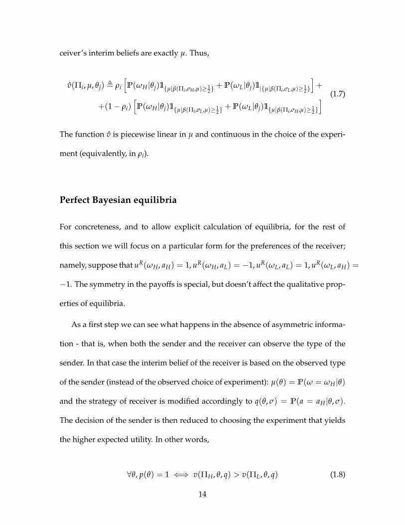
The function v is piecewise linear in µ and continuous in the choice of the experi-

ment (equivalently, in ρi).

Perfect Bayesian equilibria

For concreteness, and to allow explicit calculation of equilibria, for the rest of

this section we will focus on a particular form for the preferences of the receiver;

namely, suppose that uR(ωH, aH) = 1, uR(ωH, aL) = −1, uR(ωL, aL) = 1, uR(ωL, aH) =

−1. The symmetry in the payoffs is special, but doesn’t affect the qualitative prop-

erties of equilibria.

As a first step we can see what happens in the absence of asymmetric informa-

tion - that is, when both the sender and the receiver can observe the type of the

sender. In that case the interim belief of the receiver is based on the observed type

of the sender (instead of the observed choice of experiment): µ(θ) = P(ω = ωH|θ)

and the strategy of receiver is modified accordingly to q(θ, σ) = P(a = aH|θ, σ).

The decision of the sender is then reduced to choosing the experiment that yields

the higher expected utility. In other words,

∀θ, p(θ) = 1 ⇐⇒ v(ΠH, θ, q) > v(ΠL, θ, q) (1.8)

14

and p(θ) = 0 otherwise (ties are impossible given the different parameters and

the specification of the sender’s utility). Observe that this situation is identical to

to the model described in KG (and all the insights therein apply), except that the

sender is constrained to choose among only two experiments.

From now assume that the type of sender is privately known only to the sender.

As a first observation one can note that in any equilibrium we must have p(θH) ≥

p(θL); otherwise one would get an immediate contradiction.

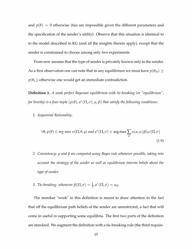
Definition 1. A weak perfect Bayesian equilibrium with tie-breaking (or "equilibrium",

for brevity) is a four-tuple (p(θ), a∗(Π, σ), µ, β) that satisfy the following conditions:

1. Sequential Rationality:

∀θ, p(θ) ∈ arg max v(Π, θ, q) and a∗(Π, σ) ∈ arg max ∑ω

u(a, ω)β(ω|Π, σ)

(1.9)

2. Consistency: µ and β are computed using Bayes rule whenever possible, taking into

account the strategy of the sender as well as equilibrium interim beliefs about the

type of sender.

3. Tie-breaking: whenever β(Π, σ) = 12 , a∗(Π, σ) = aH.

The moniker "weak" in this definition is meant to draw attention to the fact

that off the equilibrium path beliefs of the sender are unrestricted, a fact that will

come in useful in supporting some equilibria. The first two parts of the definition

are standard. We augment the definition with a tie-breaking rule (the third require-

15

ment) to facilitate and simplify the exposition. The rule requires that whenever the

receiver is indifferent between two actions, he always chooses the one preferred

by the sender10. A more substantive reason to focus on this particular tie-breaking

rule is that this makes the value function of the sender upper-semicontinuous, and

so by an extended version of the Weierstrass theorem, there will exist an experi-

ment maximizing it. This will be crucial when we consider more inclusive sets of

experiments.

For the question of existence11 of equilibria one can appeal to the fact that this

is a finite extensive game, and as such, has a trembling-hand perfect equilibrium

(Selten (1975) and Osborne and Rubinstein (1994), their Corollary 253.2), and there-

fore, has a sequential equilibrium (Kreps and Wilson (1982), and therefore has a

wPBE, since these equilibrium concepts are nested.

As usual, in evaluating the observed signal the receiver uses a conjecture of the

sender’s strategy, correct in equilibrium. Note once again that in contrast to Hed-

lund (2017), in the present model there is no experiment that fully discloses the

state of the world. If it was available, and the sender were to choose it, then the

sender’s payoffs would be independent of the receiver’s interim belief (rendering

the entire "persuasion" point moot); such an experiment would also provide uni-

form type-specific lower bounds on payoffs for the sender, since that would be a

deviation that would always be available. The fact that this is not available makes

10It is common in the literature to focus on "sender-preferred" equilibria; we do not make thesame assumption, but "bias" out equilibria in the same direction

11Even though we explicitly construct an equilibrium, and hence they certainly exist, it is usefulto have a result for more general settings.

16

the analysis more difficult, but also more interesting. The preference specification

in the present model allows us to get around the difficulty and derive analogous

results without relying on the existence of a perfectly revealing experiment.

In what follows we will focus on the interesting range of parameters π, ξ, ρH, ρL ∈

(0, 1) ×[

12 , 1)3, where the receiver takes different actions after different sig-

nals12. To that end, let

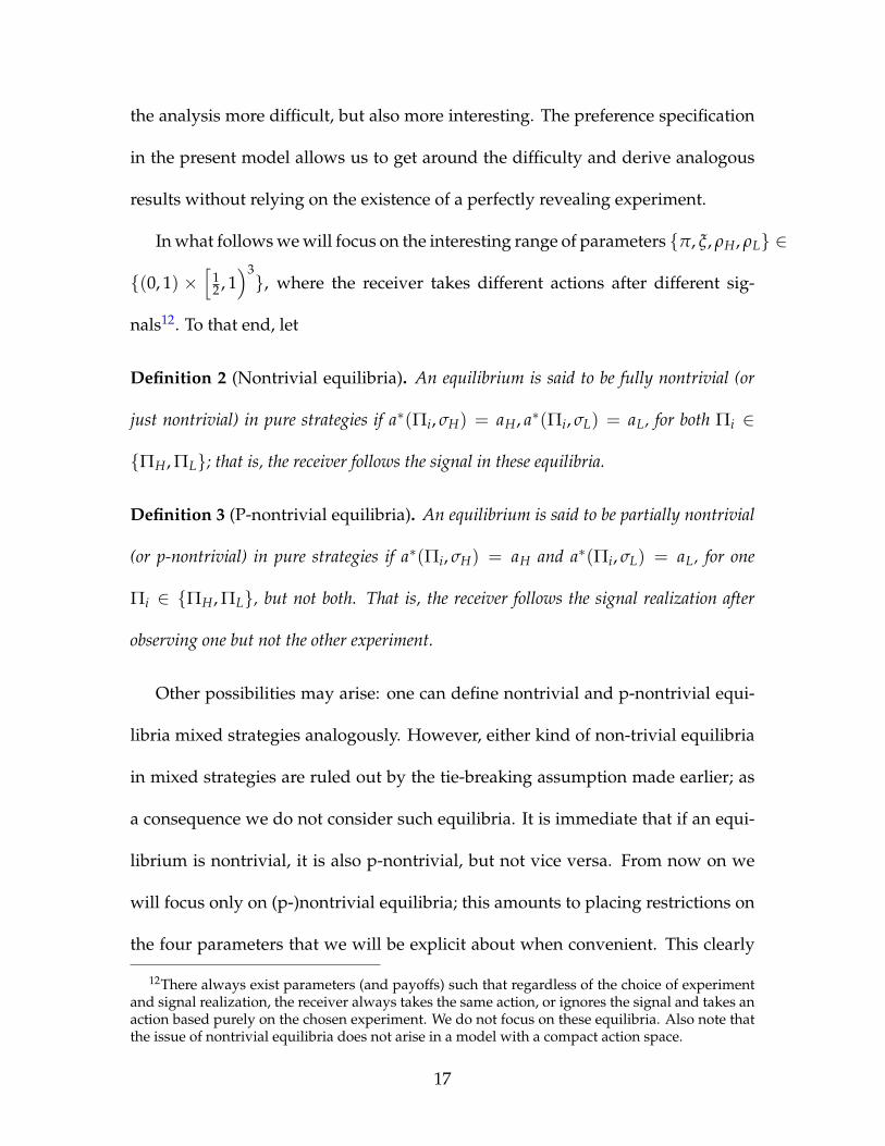
Definition 2 (Nontrivial equilibria). An equilibrium is said to be fully nontrivial (or

just nontrivial) in pure strategies if a∗(Πi, σH) = aH, a∗(Πi, σL) = aL, for both Πi ∈

ΠH, ΠL; that is, the receiver follows the signal in these equilibria.

Definition 3 (P-nontrivial equilibria). An equilibrium is said to be partially nontrivial

(or p-nontrivial) in pure strategies if a∗(Πi, σH) = aH and a∗(Πi, σL) = aL, for one

Πi ∈ ΠH, ΠL, but not both. That is, the receiver follows the signal realization after

observing one but not the other experiment.

Other possibilities may arise: one can define nontrivial and p-nontrivial equi-

libria mixed strategies analogously. However, either kind of non-trivial equilibria

in mixed strategies are ruled out by the tie-breaking assumption made earlier; as

a consequence we do not consider such equilibria. It is immediate that if an equi-

librium is nontrivial, it is also p-nontrivial, but not vice versa. From now on we

will focus only on (p-)nontrivial equilibria; this amounts to placing restrictions on

the four parameters that we will be explicit about when convenient. This clearly

12There always exist parameters (and payoffs) such that regardless of the choice of experimentand signal realization, the receiver always takes the same action, or ignores the signal and takes anaction based purely on the chosen experiment. We do not focus on these equilibria. Also note thatthe issue of nontrivial equilibria does not arise in a model with a compact action space.

17

doesn’t cover all possible equilibria for all possible parameters, but it does focus

on the "interesting" equilibria. The following straightforward propositions serve

to narrow down the set of possible equilibria.

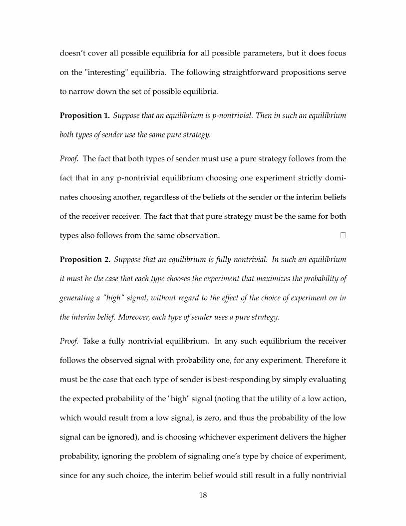
Proposition 1. Suppose that an equilibrium is p-nontrivial. Then in such an equilibrium

both types of sender use the same pure strategy.

Proof. The fact that both types of sender must use a pure strategy follows from the

fact that in any p-nontrivial equilibrium choosing one experiment strictly domi-

nates choosing another, regardless of the beliefs of the sender or the interim beliefs

of the receiver receiver. The fact that that pure strategy must be the same for both

types also follows from the same observation.

Proposition 2. Suppose that an equilibrium is fully nontrivial. In such an equilibrium

it must be the case that each type chooses the experiment that maximizes the probability of

generating a "high" signal, without regard to the effect of the choice of experiment on in

the interim belief. Moreover, each type of sender uses a pure strategy.

Proof. Take a fully nontrivial equilibrium. In any such equilibrium the receiver

follows the observed signal with probability one, for any experiment. Therefore it

must be the case that each type of sender is best-responding by simply evaluating

the expected probability of the "high" signal (noting that the utility of a low action,

which would result from a low signal, is zero, and thus the probability of the low

signal can be ignored), and is choosing whichever experiment delivers the higher

probability, ignoring the problem of signaling one’s type by choice of experiment,

since for any such choice, the interim belief would still result in a fully nontrivial

18

equilibrium, by assumption. Ties are impossible due to the different precision of

experiments and different sender beliefs, hence the focus on pure strategies.

The above two propositions taken together eliminate the possibility of mixing

for the sender. The following propositions state all possible equilibria; they are

supported, as is standard, by beliefs that assign probability one to off-path devia-

tions coming from the low type of sender. Incentive compatibility can be proven

by directly computing utilities on and off the equilibrium path, and verifying best

responses, using Bayes rule whenever possible. We omit the tedious but straight-

forward computations. For convenience, for any variable x ∈ (0, 1) denote by x

the ratio x1−x .

We present the formal results on equilibriua in the sequence of propositions

that follows. In short, there are both pooling and separating equilibria (and we

give the conditions for their existence), and importantly, the pooling can be on the

less informative equilibrium. This is in sharp contrast to the work of Hedlund

(2017). In a model with more actions that is studied in later sections there are also

pooling equilibria on every experiment.

Proposition 3. There is a unique separating equilibrium where p(θH) = 1, p(θL) = 0.

This equilibrium exists as long as π, ξ, ρH, ρL satisfy equations the following restric-

tions: π ≤ ξ, π + ξ > 1, π ˜ρH ξ > 1, ˜ρH > πξ, πρL > ξ, ρLξ > π. Denote this

equilibrium by "SEP".

Intuitively, in this equilibrium the low type of sender prefers to "confuse" the

receiver by sending a sufficiently uninformative signal. We now turn to classifying

19

pooling equilibria.

Proposition 4. There is a continuum of fully nontrivial pooling equilibria where p(θH) =

p(θL) = 1. These equilibria exist as long as π + ξ ≥ 1, π ≥ ξ, π ˜ρH ≥ 1, ρH > π, πρL ≥

ξ, ρLξ > π. The only difference between these equilibria are the beliefs that the receiver

holds off-path; namely, µ(ΠL) ∈ [P(ωH|θL), ρL). Denote this kind of equilibria by "FNT-

H".


p(θL) = 0. These equilibria exist as long as π + ξ ≤ 1, π ≤ ξ, π ˜ρH ξ ≥ 1, ρL > π, ρL >

ξπ, ρLπ ≥ 1. The only difference between these equilibria are the beliefs that the receiver

holds off-path; namely, µ(ΠH) ∈ [P(ωH|θL), ρH). Denote this kind of equilibria by

"FNT-L".

Proposition 6. There is a continuum of p-nontrivial pooling equilibria where p(θH) =

p(θL) = 1, a∗(ΠL, σ) = aL, for σ = σH, σL, and a∗(ΠH, σH) = aH, a∗(ΠH, σL) = aL..

These equilibria exist as long as ξ > ρLπ, ρH > π, and π + ρH ≥ 1. The only difference

between these equilibria are the beliefs that the receiver holds off-path; namely, µ(ΠL) ∈

[P(ωH|θL), 1− ρL). Denote this kind of equilibria by "PNT-HL(aL)"13.


p(θL) = 1, a∗(ΠH, σ) = aH, for σ = σH, σL and a∗(ΠL, σH) = aH, a∗(ΠL, σL) =

aL. These equilibria exist as long as ρLπ ≥ ξ, ρH ≥ π, π < ξ ρL. The only difference

13For any PNT equilibrium, the notation "PNT-XY(ai)" equilibrium denotes the fact that thesenders pool on experiment X, and the receiver takes the same action after observing experimentY, for X, Y = H, L, ai ∈ aH , aL.

20

between these equilibria are the beliefs that the receiver holds off-path; namely, µ(ΠL) ∈

[P(ωH|θL), ρL). Denote this kind of equilibria by "PNT-HH(aH)".


p(θL) = 0, a∗(ΠL, σH) = aH, a∗(ΠL, σL) = aL and a∗(ΠH, σ) = aL, for σ = σH, σL.

These equilibria exist as long as ρL > π, ρL + π ≥ 1 and ˜ρHπ < ξ. The only difference

between these equilibria are the beliefs that the receiver holds off-path; namely, µ(ΠH) ∈

[P(ωH|θL), 1− ρH). Denote this kind of equilibria by "PNT-LH(aL)".


p(θL) = 0, a∗(ΠL, σ) = aH, for σ = σH, σL and a∗(ΠH, σH) = aH, a∗(ΠH, σL) = aL.

These equilibria exist as long as ˜ρHπ ≥ ξ, ρL ≤ π, π ≤ ξ ˜ρH. The only difference

between these equilibria are the beliefs that the receiver holds off-path; namely, µ(ΠH) ∈

[P(ωH|θL), 1− ρL). Denote this kind of equilibria by "PNT-LL(aH)".

These are all the equilibria of this game14. The following proposition, which

can be verified by direct computation15, shows that some of these equilibria16 can

coexist in the sense that for some set of parameters, both types of equilibria occur:

Proposition 10. There are sets of parameters for which the following types of equilibria

coexist (i.e. both can occur):

1) PNT-HL(aL) and PNT-LH(aL).

14It can be checked directly that there are no "perverse" equilibria where the receiver "inverts"the signal (that would never be optimal) or another separating equilibrium where the high typepretends to be the low type and vice versa.

15Using, for example, a computer algebra system such as Mathematica and checking for exis-tence of solutions to the various inequalities determining the existence of different equilibria.

16There are other results on (non-)coexistence of various types of equilibria; we list only the onesthat are relevant.

21

2) PNT-HH(aH) and PNT-LL(aH).

3 FNT-H and FNT-L.

4) FNT-H and PNT-HH(aH).

5) SEP and PNT-HH(aH).

Typically, the question of coexistence of equilibria does not come up, since all of

them always coexist (for example, in the Cho-Kreps beer-quiche game or Spencian

signaling); they are, however, important in this setting since we will eventually

apply refinements to select among these equilibria. If one views a refinement as

simply a condition that a particular equilibrium may satisfy or not, the question

of coexistence is irrelevant. If one views a refinement as a prediction of which

of several equilibria is more plausible, one can conceivably say that if they do

not coexist, one does not need a refinement to choose among equilibria, since the

conditions for existence of an equilibrium will function as a kind of refinement (as

is the case here). In either case, we show that the relevant equilibria do, in fact,

coexist, so that applying a refinement has meaning.

Either the different kinds of equilibria do not coexist, or, if they do, a novel

refinement will help select among them in interesting cases.

Discussion and Refinements

There are a number of notable differences between this simple model and the mod-

els presented by Hedlund (2017), Perez-Richet (2014) and Degan and Li (2015);

one is the types of equilibria they admit. In Perez-Richet (2014)’s model separat-

22

ing equilibria are only possible when there exists a fully revealing experiment;

otherwise all equilibria are pooling. In Hedlund (2017)’s model equilibria17 are ei-

ther pooling on the fully revealing experiment or fully separating where all types

choose different experiments in equilibrium; furthermore the pooling and sepa-

rating equilibria do not coexist. In the model discussed here nontrivial separating

(in contrast to Perez-Richet (2014)) and equilibria where the pooling is on the less

informative signal, as well as the striking feature of coexisting pooling and sepa-

rating equilibria (in contrast to Hedlund (2017)) are possible. If, in addition, we

dispense with the tie-breaking rule that is part of the present model, another, hy-

brid, type of equilibrium is possible, one where the type of sender randomizes,

while the other plays a pure strategy. This type of equilibrium is not possible in

either of the two alternative models. Degan and Li (2015) work in a setting that

is similar to Perez-Richet (2014)’s, but posit type-independent costly signals; their

results on the types of possible equilibria are analogous - in particular, there exists

a unique separating equilibrium (which does not survive a refinement - D1 - which

we also define shortly) in their model, and a number of pooling equilibria (which

may or may not survive D1).

Previous work has also characterized equilibria of various models; in addition,

owing to the fact that typically there are a large number of equilibria, various re-

finements have been brought to bear on the results, in order to obtain sharper pre-

dictions18. The most common refinement is criterion D1; we now give a suitably

17He focuses on equilibria that also satisfy a refinement - criterion D1. In the present model thisrefinement does not make any predictions beyond those of PBE with tie-breaking.

18Typically in cheap-talk games refinements based on stability have no bite since messages are

23

modified variant of its definition:

Definition 4 (Criterion D1). Fix an equilibrium p∗, q∗, µ∗, β∗, and let u∗S(θ) the the

equilibrium utility of each type of sender. For out-of-equilibrium pairs (Π ′, µ), let

D0(Π ′, θ) , µ ∈ [P(ωH|θL), P(ωH|θH)]|u∗(θ) = v(Π, µ∗, θ) ≤ v(Π ′, µ, θ)], and

D(Π ′, θ) , µ ∈ [P(ωH|θL), P(ωH|θH)]|u∗(θ) = v(Π, µ∗, θ) < v(Π ′, µ, θ)]. A

PBE is said to survive criterion D1 if there is no θ ′ s.t.

D(Π ′, θ) ∪ D0(Π ′, θ) ( D(Π ′, θ ′) (1.10)

Typically in signaling models this criterion is defined somewhat differently - in

terms of receiver best responses, rather than beliefs; it is without loss in this setting

to use this definition (see also Hedlund (2017)). In addition, it is usually defined

using beliefs of the receiver about the type of the sender (here, ν), rather than the

state of the world (µ) - this is due to the fact that in most other models, these are

one and the same, while here they are distinct, and what matters for the payoff is

the state of the world, hence the definition must be given in terms of that.

It can be checked by direct computation that all of the equilibria described

above survive criterion D1, and thus, it does not help refine predictions beyond

costless. The standard argument for why that is true goes as follows: suppose that there is anequilibrium where a message, say m ′ is not sent, and another message, m, is sent. Then we canconstruct another equilibrium with the same outcome where the sender randomizes between mand m ′ and the beliefs of the receiver upon observing m ′ are the same as his beliefs upon observingm in the original equilibrium. Here this is not true - although all experiments are costless, theygenerate different signals with different probabilities. For the sender to be mixing she must beindifferent between both experiments, but given the different probabilities that is impossible, andtherefore we cannot support all equilibria by mixing. Thus refinements based on stability andrestricting beliefs "regain" their bite in this setting.

24

those of PBE with tie-breaking19. This is due to the fact that for all equilibria and

deviations, criterion D1 requires a strict inclusion of the D sets, as emphasized in

equation 1.10, while in this game the relevant D sets are, in fact, identical for both

types. Similarly, other related refinements such as the intuitive criterion20 and

other refinements based on strategic stability Kohlberg and Mertens (1986).

Other standard refinements for signaling games such as perfect sequential equi-

libria (Grossman and Perry (1986)), neologism-proof equilibria (Farrell (1993))21,

or perfect (Selten (1975)) or proper (Myerson (1978)) equilibria, also do not narrow

down predictions, for similar reasons.

Finally, another refinement concept - undefeated equilibria (Mailath et al. (1993))

- does help refine equilibria somewhat. That refinement is defined for sequential

equilibria, and it can be checked that all wPBE in this game can be sequential equi-

libria. Undefeated equilibrium still does not go far enough, as we will discuss after

modifying the model in the succeeding sections.

The other related models have features that circumvent the problem of nonre-

finability - in Hedlund (2017), it is the fact that the receiver’s action is in a compact

set, that the receiver’s action is strictly increasing in the final belief, and the fact

19Intuitively, D1 does not help due to the following: consider an equilibrium (and associatedutility levels), and a deviation. The set of receiver beliefs that make one or both types better offis the set of beliefs for which the receiver takes the high action "more often" than in the referenceequilibrium. But the set of these beliefs is identical for both types, since the receiver’s utility onlydepends on the state of the world, and not on the type of the receiver.

20The reason this refinement does not work is that for the right range of beliefs both types bene-fit. Note also that were this not true, we would be in the range of parameters where the separatingequilibrium occurs - c.f. SEP.

21Both of these two refinements also fail since both types benefit from a deviation under thesame set of beliefs.

25

that the sender’s utility is strictly increasing in the receiver’s action22; in Perez-

Richet (2014) it is the fact that sender is perfectly informed and the fact that the

receiver can use mixed strategies; in Degan and Li (2015) it is the fact that the ac-

tion of the sender (the message) is continuous and related to the precision of the

signal observed by the receiver. We will say more about the differences between

the present setting and others below.

There is, however, another, novel, refinement that we can define. Take for ex-

ample the PNT-LH(aL) equilibrium; one may notice that while other refinement

concepts do not work well, there is a curious feature in this equilibrium. It is this:

while neither type benefits from a deviation to ΠH under the equilibrium beliefs,

and both types benefit from the same deviation under other, non-equilibrium be-

liefs, it is the high type that benefits relatively more. This observation suggests a

refinement idea - one may restrict out-of-equilibrium beliefs to be consistent not

just with the types that benefit (such as the intuitive criterion, neologism-proof

equilibria and others) or sets of beliefs (or responses) of the sender for which cer-

tain types benefit (such as stability-based refinements), but also with the relative

benefits from a deviation23. It is also hoped that this refinement will prove useful

in other applications where other refinements perform poorly.

This idea is also connected to the idea of trembles (Selten (1975)); namely that

if one thinks of deviations from equilibrium as unintentional mistakes, this can be

accommodated by the present refinement, but with an additional requirement -

22We discuss in detail the differences between Hedlund’s model and ours below.23We further explore the implications, properties and performance of this criterion in related

contemporaneous work.

26

the player for whom the difference between the equilibrium utility and the "trem-

ble utility" is greater should tremble more, and therefore, the beliefs of the receiver

should that that into account. A similar reasoning (albeit in a different setting) is

also present in the justification for quantal response equilibrium (QRE) of McK-

elvey and Palfrey (1995) where players may tremble to out-of-equilibrium actions

with a frequency that is proportional in a precise sense to their equilibrium utility.

These ideas are also what is behind the nomenclature - BPM stands for Belief-

Payoff Monotonicity. We now turn to this refinement, and show that it does help

narrow down the predictions to some degree. We give a definition that is suitable

to the present environment, but it can be generalized in a straightforward way.

Definition 5 (Criterion BPM). Let p∗, q∗, µ∗, β∗ be an equilibrium and let u∗(θ) be

the equilibrium utility of type θ. Define, for a fixed θ and Πi, v(θi) , maxa,µ v(Πi, θi, µ)

and v(θi) , mina,µ v(Πi, θi, µ). An equilibrium is said to fail criterion BPM if there is

an experiment Πi, not chosen with positive probability in that equilibrium and a type of

sender, θj, such that:

i) Let µ ∈ ∆(Ω) be an arbitrary belief of the receiver and suppose that δ(Π, µ, θi, e) ,

v(Π,θi,µ)−u∗(θi)v(θi)−v(θi)

> 0, for that belief.

ii) Denote by K be the set of types for which (i) is true. Let θi be the type for which

the difference is greatest. If there is another type θj in K, for which δ(Π, µ, θi, e) >

δ(Π, µ, θj, e) then let µ(θj|Π) < εµ(θi|Π), for some positive ε, with ε < 1|K| . If

there is another type θk such that δ(Π, µ, θj, e) > δ(Π, µ, θk, e), then let µ(θk|Π) <

εµ(θj|Π), and so on.

27

iii) Beliefs are consistent: given the restrictions in (ii), the belief µ is precisely the beliefs

that makes (i) true.

We say that an equilibrium fails the BPM criterion if it fails the ε-BPM criterion

for every admissible ε. In words, criterion BPM restricts out-of-equilibrum beliefs

of the receiver in the following way: if there are beliefs about off-equilibrium path

deviations, for which one type benefits more than another, then equilibrium beliefs

must assign lexicographically larger probability to the deviation coming from the

type that benefits the most. We also scale the differences in a way that makes the

definition ordinal (see also de Groot-Ruiz et al. (2013)). Note also that the second

part of the definition looks very much like a condition of increasing differences;

this is indeed so and purposeful. In addition, one can note that for utility functions

which do satisfy increasing differences, criterion BPM would generate meaningful

and intuitive belief restrictions.

The definition given above is ordinal (i.e., for any sender’s vNM utility function

u(x) the definition has the same meaning if u(x) was replaced by v(x) = a+ bu(x),

for any real number a and any positive real number b).

From now on we will refer to a PBE with tie-breaking that also survives crite-

rion BPM as a BPM equilibrium. We have the following proposition:

Proposition 11. The following classes of equilibria are BPM equilibria: SEP, FNT-H,

FNT-L, PNT-HL(aL), PNT-HH(aH) and PNT-LL(aH).

In other words, this proposition applies to parts 1 and 3 of proposition 10, and

makes a selection between the coexisting equilibria mentioned there. It should

28

be noted that these equilibria are also ε-BPM equilibria, for all admissible ε, but

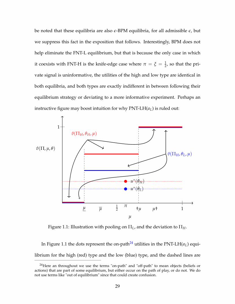
we suppress this fact in the exposition that follows. Interestingly, BPM does not

help eliminate the FNT-L equilibrium, but that is because the only case in which

it coexists with FNT-H is the knife-edge case where π = ξ = 12 , so that the pri-

vate signal is uninformative, the utilities of the high and low type are identical in

both equilibria, and both types are exactly indifferent in between following their

equilibrium strategy or deviating to a more informative experiment. Perhaps an

instructive figure may boost intuition for why PNT-LH(aL) is ruled out:

1

v(Π, µ, θ)

µ

µ µ †µ µ†12 1

π

u∗(θL)

u∗(θH)

v(ΠH, θH, µ)

v(ΠH, θL, µ)

Figure 1.1: Illustration with pooling on ΠL, and the deviation to ΠH.

In Figure 1.1 the dots represent the on-path24 utilities in the PNT-LH(aL) equi-

librium for the high (red) type and the low (blue) type, and the dashed lines are

24Here an throughout we use the terms "on-path" and "off-path" to mean objects (beliefs oractions) that are part of some equilibrium, but either occur on the path of play, or do not. We donot use terms like "out of equilibrium" since that could create confusion.

29

there to make the comparisons of utilities from deviations easier; the equilibrium

utility of deviating in that equilibrium is zero given the beliefs. The solid lines

represent the expected utility of deviating to a more informative experiment as a

function of the interim beliefs of the receiver; the differences between the solid

and the dashed lines are computed in the proof above, for each µ. Clearly, for

µ ∈ [0, µ)25 both types get zero payoff from the deviation, since for those beliefs

the receiver always takes the low action. Criterion BPM does not apply there since

neither type benefits from such a deviation for those beliefs. The crucial region is

µ ∈ [µ, †µ). It is here that criterion BPM operates efficiently - both types get posi-

tive payoff from the equilibrium and the deviation, but we have shown above that

the high type benefits relatively more. And beliefs above µ†, again, cannot sustain

a nontrivial equilibrium and hence we do not have to consider them since they lie

outside the scope of admissible beliefs.

There is a small but important subtlety to be noticed - in any equilibrium (pool-

ing or otherwise), u∗S(θH) ≥ u∗S(θL), because the private information of the sender

(her type) forces the high type of the sender to have higher beliefs about the prob-

ability of higher signals, since P(σH|θH) > P(σH|θL). Nevertheless, given the re-

strictions on parameter discussed above, BPM does, in fact eliminate the equilibria

where both types pool on the less informative experiments (with the exception of

PNT-LL(aH)); the reason it does not eliminate that equilibrium is because there, on

the equilibrium path, the sender gets the highest possible utility she can get with

25Note that the right boundary is not included, since at that point the receiver would switch totaking the high action, by assumption.

30

probability one. Thus, no reasonable refinement could ever refine that outcome

away, since the sender would never deviate from the equilibrium. As mentioned

above, undefeated equilibrium does help to refine predictions, however, and in

fact, makes a very similar selection.

Finitely many actions for the receiver and finitely many types for the sender can

be accommodated easily in our setting; while we do not present explicit results to

that end, it is straightforward to see that the same equilibria can exist in such an

environment. We study an extension with an uncountable number experiments in

the next section and show that analogous results continue to exist. Finally, to show

that the results in our model do not depend on the absence of a fully revealing ex-

periment, we explore this possibility. Interestingly, making ΠH be fully revealing

in the present setting (i.e. setting ρH = 1) does not make much of a difference.

Differences with the model of Hedlund: modeling assumptions

and results.

As mentioned above, the model of Hedlund (2017) is rather close to the one dis-

cussed here; yet the predictions are sufficiently distinct. We now turn to a more

detailed discussion of the differences (and similarities) between the models, as

well as the implications of those differences for equilibria.

The most notable difference is that our model can support both pooling and

separating equilibria, and even in BPM equilibria we can get pooling on the less

31

informative experiment26. In addition, number of features of the equilibria in

Hedlund (2017)’s model fail here; notably, the fact that in equilibrium the senders

choose more informative experiments than they would have under symmetric in-

formation, as well as the fact that the payoff for senders is the same across all

equilibria.

Finitely many actions for the receiver and finitely many types for the sender can

be accommodated easily in our setting; while we do not present explicit results to

that end, it is straightforward to see that the same equilibria can exist in such an

environment. We study an extension with an uncountable number experiments in

the next section and show that analogous results continue to exist.

The assumptions that are responsible for these differences can be divided into

two classes - assumptions about the actions available to the sender (i.e. the set of

experiments), and assumptions about the utilities of the players as well as the ac-

tions available to the receiver. Changing the assumptions in either class will result

in equilibria that are qualitatively closer to the equilibria of this model (notably,

producing nontrivial pooling equilibria).

Consider first the assumptions regarding the set of available experiments. First

of all, if the fully revealing experiment is not available in Hedlund (2017)’s model,

the same results may not hold27; it should be noted that Perez-Richet (2014) also

finds that absent a fully revealing experiment, there exist many PBEs, just like in

the model we study. Another assumption is that all possible experiments are avail-

26Recall that in Degan and Li (2015)’s model the D1 equilibria are also pooling.27It is not clear whether they do or do not but Hedlund’s characterization would not apply.

32

able to the sender, or equivalently, she can freely design them. This is crucial since

some of the results rely on such a constructed experiment. Moreover, as men-

tioned above, a fully revealing experiment is independent of the interim beliefs of

the receiver (and thus the signaling element of the model is "shut down"); the mere

presence of this deviation for the receiver has significant consequences, even if it

is not an action that is taken in equilibrium. However, suppose that we take Hed-

lund (2017)’s model and remove all experiments except for two - a fully revealing

one, and an arbitrary other one. Then, if the common prior that the state is high

is sufficiently close to 1, it will be an equilibrium for both types of sender to pool

on the non-fully revealing experiment; moreover, this equilibrium will survive cri-

terion D1, since both D0 and D sets are empty. Thus, dropping the assumptions

about the set of available experiments results in equilibria that are similar to the

equilibria studied here.

Consider now the second class of assumptions. Among other differences be-

tween these models there are three key ones: i) a connected action space for the

receiver, ii) the fact that the sender’s utility is strictly increasing in the action of

the receiver and iii) the fact that the receiver’s best response is strictly increasing

in the final belief. All three of these assumptions are not satisfied in the present

setting. It is this combination of assumptions taken together that is responsible

for the differences in results and predictions between the two models. We now

show by examples that dropping any one of these four assumptions (but keeping

the other three), and thus introducing some "coarseness" into the setting, would

change the results of Hedlund (2017) significantly, elegant though they may be,

33

and bring them closer to the results in this model.

One can also drop the assumption of a connected action set for the receiver:

for convenience suppose that there are two types of sender, any finite number of

available actions for the receiver and all other assumptions are the same as in Hed-

lund (2017). In this case the finite number of actions forces the possible utilities of

the sender and receiver to also take on a finite number of values (and in addition,

the receiver’s optimal action can no longer be strictly increasing in his final be-

lief, which is a key element in Hedlund (2017)) - therefore this effectively becomes

analogous to the model studied in the present work, with all of the resulting con-

clusions.

Similarly, keeping a connected action space, and making aR(β) (the optimal

action of the receiver as a function of his final belief) constant over some regions28,

or keeping aR(β) strictly increasing but making the sender’s utility constant over

some regions of the receiver’s actions makes Hedlund (2017)’s results break down.

Welfare and Comparative Statics

We now turn to the question of welfare. For the receiver29, the expected utility

is the same across the FNT-H and PNT-HL(aL) equilibria, and equal to 2ρH − 1,

which is positive by assumption. His utility from the equilibria FNT-L and PNT-

LH(aL) is strictly lower than that and equal to 2ρL − 1. His utility from PNT-

28If this function is decreasing over some regions the model changes significantly, since then thepreferences of the receiver are no longer about matching the state as closely as possible; we do notconsider this case.

29Note that for the specific utility function posited for the receiver, the expected utility of thereceiver is also numerically equivalent to the probability of making the correct decision.

34

HH(aH) and PNT-LL(aH) is 2π − 1. His utility from SEP is (ρH − ρL)(3πξ − 2π −

2ξ) + 2ρH − 1; this can be positive or negative even in the range of relevant pa-

rameters. Thus among the pooling equilibria the receiver prefers the more infor-

mative one, and how he ranks the separating one is ambiguous. An interesting

comparison is between the receiver’s payoff in these equilibria and his payoff in

the absence of any persuasion - that is, what the receiver would do based just on

the prior. Clearly, if the prior is π ≥ 12 the receiver should take the high action,

yielding a payoff of 2π − 1 and if π < 12 , the receiver should choose the low ac-

tion, and obtain 1− 2π in expectation. One can definitely say in this case that if

π ≥ 12 (and so, ex ante, the interests of the receiver and the sender are aligned),

and the rest of the parameters are such that any type of pooling equilibrium ob-

tains, the receiver strictly prefers the outcome under persuasion over that under

no persuasion. This is a rather interesting result, showing that even if the sender

always prefers one of the outcomes, the receiver may still prefer to be persuaded.

Other utility comparisons are, again, ambiguous.

As for the sender, we can say that in any equilibrium, the expected utility of the

high type is always weakly greater than that of the low type. Clearly the payoff

for both types from PNT-HH(aH) and PNT-LL(aH) is equal to unity. The high type

of sender obtains the same expected payoff from FNT-H, PNT-HL(aL) and SEP;

that payoff is equal to ρHπξ+(1−ρH)(1−π)(1−ξ)πξ+(1−ξ)(1−π)

. Her expected payoff from FNT-L

and PNT-LH(aL) is equal to ρLπξ+(1−ρL)(1−π)(1−ξ)πξ+(1−ξ)(1−π)

. As for the low type, her pay-

off from SEP, FNT-H, and PNT-HL(aL) is ρHπ(1−ξ)+ξ(1−ρH)(1−π)π(1−ξ)+ξ(1−π)

, and that FNT-L

35

and PNT-LH(aL) is: ρLπ(1−ξ)+ξ(1−ρL)(1−π)π(1−ξ)+ξ(1−π)

. Comparing these expected payoffs is

more difficult, since they involve all four parameters and different equilibria occur

under different parameters; thus, it is not possible to say in general, which type

of equilibrium each type prefers. However, when equilibria do coexist, the util-

ity of FNT-H is higher than that of FNT-L for both types, and the same is true of

PNT-HL(aL) and PNT-LH(aL). Thus, when it does make nontrivial selections, BPM

picks out equilibria that are preferred by both the sender and the receiver. While

BPM does not make a selection among PNT-HH(aH) and PNT-LL(aH), the sender

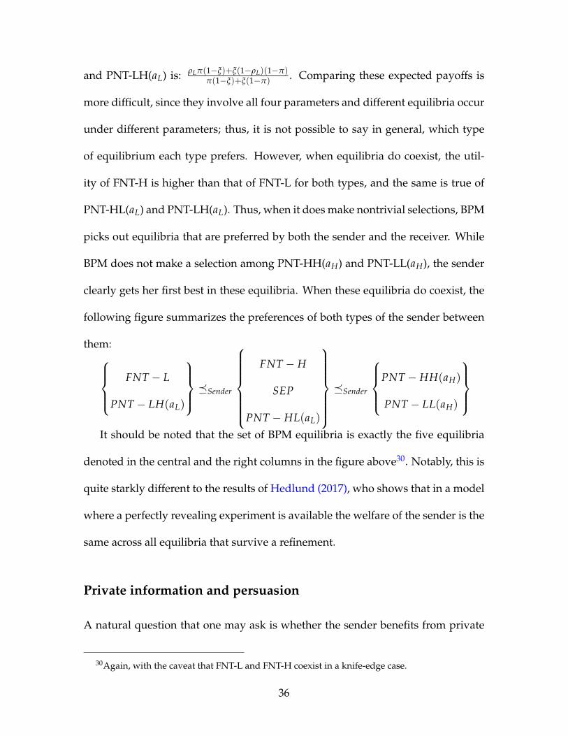
clearly gets her first best in these equilibria. When these equilibria do coexist, the

following figure summarizes the preferences of both types of the sender between

them:FNT − L

PNT − LH(aL)

Sender

FNT − H

SEP

PNT − HL(aL)

Sender

PNT − HH(aH)

PNT − LL(aH)

It should be noted that the set of BPM equilibria is exactly the five equilibria

denoted in the central and the right columns in the figure above30. Notably, this is

quite starkly different to the results of Hedlund (2017), who shows that in a model

where a perfectly revealing experiment is available the welfare of the sender is the

same across all equilibria that survive a refinement.

Private information and persuasion

A natural question that one may ask is whether the sender benefits from private

30Again, with the caveat that FNT-L and FNT-H coexist in a knife-edge case.

36

information in this setting - that is, whether the sender would ex-ante prefer to

be informed or not. Without private information this model is identical to the

model of KG, except for the available experiments. Without private information

it also doesn’t make sense to speak of the "type" of sender in this situation; there-

fore, without observing a private signal the sender would simply choose the more

informative experiment, if the common prior π is above one half, and less infor-

mative experiment otherwise. The expected payoff for the sender would be equal

to ρHπ + (1− ρH)(1− π), which is in between that of the high type and the low

type. Thus we can conclude that the sender sometimes benefits from private infor-

mation. This is in in line with Alonso and Camara (2016) who show that if a fully

revealing experiment is available, the sender does not benefit from private infor-

mation. In addition to lacking a fully revealing experiment, in this setting the pri-

vate information of the sender is also not "redundant" in the sense that Alonso and

Camara make precise in their work; this feature also allows an informed sender to

be better or worse off. We also note that here the sender does not benefit from per-

suasion31 (and in fact does strictly worse), if the receiver is ex-ante willing to take

the high action (i.e. if π ≥ 12 ), and does strictly better otherwise. This observation

has an analogue in KG - there, also, the sender benefits if the receiver is be willing

ex-ante take an action that is inferior from the point of view of the sender.

31In the sense of KG - that is, if the value function of the sender evaluated at the prior is greaterthan the expected payoff at the prior in the absence of any persuasion.

37

Summary of Results on the Basic Model

Among the contributions is a result on informativeness of equilibria. Contrary to

previous work, private information matters in this setting. Equilibria may or may

not be very informative. However, we define a new refinement that selects the

most informative equilibria, except for special cases. The special cases fall under

two umbrellas; either the pooling is on the less informative experiment, but the re-

ceiver is taking the best possible action after observing that experiment (regardless

of the realization of the signal!). This equilibrium cannot be refined away by our

concept (or indeed, by any reasonable existing concept) since here although the

equilibrium is not very informative, the sender still gets her fist best utility on the

equilibrium path, and thus has no incentive to deviate - ever, regardless of what

the receiver may conceivably believe. The second class of less informative pool-

ing equilibria - FNT-L - only coexists with FNT-H in a knife-edge, degenerate case

where the private signal is completely noisy, and all types of sender are indiffer-

ent between everything. This less informative equilibrium also cannot be refined

away, but again, not for a substantial reason.

Going Further: More Available Experiments

Armed with the setup and intuition from the preceding discussion, we can go

somewhat further and dispense with arbitrarily restricting the set of available ex-

periments to just two.

Suppose instead that a finite set of experiments was available, with the ele-

38

ments of that set still ranked according to the "more informative than" criterion

(defined below). From the point of view of qualitative analysis, it is immaterial

exactly how many experiments there are, as long as there are a finite number of

them (and at least two) - the basic results about existence of a separating equilib-

rium and several types of pooling equilibria (one for each available experiment),

along with the corresponding beliefs and parameter restrictions go through with

the obvious adjustments. We do not present explicit results to that end.

Instead, consider now an uncountable set of experiments Π and endow it with

the sup norm; suppose it is a closed and compact (in the natural topology associ-

ated with the sup norm) set, still ranked. More precisely, consider the set of 2× 2

symmetric matrices that are parametrized by a single number - the probability of

a correct signal in a state, denoted by ρi. Say that Πi a generic experiment, letting

i ∈ I be some index set, and define a "more informative than"32 order on the set of

experiments as follows: if i′ 6= i, Πi ′ Πi if and only if 1 > ρi ′ > ρi >

12 . Denote

by ρa , minρ Π and ρb , maxρ Π, so that I = [a, b] ⊂ R and let ΠA and ΠB be

the corresponding experiments. Also, modify notation from the previous section

slightly as follows: let p(θ) ∈ Π and p(θ) ∈ ∆(Π). Note that Π is convex (so that

the existence result from the previous section applies).

Surprisingly, there are still only two classes of FNT pooling equilibria, one

where pooling is on the most informative experiment and one where it is on the

least informative one. This is due to the fact that the conditions for each type

32This order is coarser (i.e. a subset of) both the "more precise than" order used by Hedlund, aswell as Blackwell’s standard order.

39

of sender that ensure no deviation from a particular Πi upward (toward a more

informative experiment) and downward (toward a less informative one) are in-

compatible (within the class of FNT equilibria), and thus, no equilibrium where

the pooling is on Πi s.t. a < i < b exists.


p(θL) = Πb. These equilibria exist as long as π + ξ ≥ 1, π ≥ ξ, πρb ≥ 1, ρb >

π, πρL ≥ ξ, ρi ξ > π, ∀i ∈ I \ b. The only difference between these equilibria are the be-

liefs that the receiver holds off-path; namely, µ(Πi) ∈ [P(ωH|θL), ρa) for i 6= b. Denote

this kind of equilibria by "FNT-b".


p(θL) = Πa. These equilibria exist as long as π + ξ ≤ 1, π ≤ ξ, πρi ξ ≥ 1, ∀i ∈

I \ a, ρa > π, ρa > ξπ, ρaπ ≥ 1. The only difference between these equilibria are the be-

liefs that the receiver holds off-path; namely, µ(Πi) ∈ [P(ωH|θL), ρb) , for i 6= a. Denote

this kind of equilibria by "FNT-a".

There is also a unique separating equilibrium, which is analogous to the one

constructed above.

Proposition 14. There is a unique separating equilibrium where p(θH) = Πb, p(θL) =

Πa. This equilibrium exists as long as π ≤ ξ, π + ξ > 1, πρbξ > 1, ρb > πξ, πρa >

ξ, ρaξ > π. Denote this equilibrium by "SEP2".

The reason that this is the only separating equilibrium is this. Suppose, to the

contrary that there was another separating equilibrium, one where at least one

40

type chose p(θ) = Πi, for Πi /∈ Πa, Πb. Since the equilibrium is separating, that

type would also reveal itself by it’s choice, and thus µ(Πi) = P(ωH|θ). The choice

of that type of sender would then be

maxΠi

v(Πi, θ, P(ωH|θ)) (1.11)

or, equivalently, given the structure of available experiments,

maxρi

ρi

[P(ωH|θ)1µ|β(Πi,σH ,µ)≥ 1

2+ P(ωL|θ)1|µ|β(Πi,σL,µ)≥ 1

2

]+

+(1− ρi)[P(ωH|θ)1µ|β(Πi,σL,µ)≥ 1

2+ P(ωL|θ)1µ|β(Πi,σH ,µ)≥ 1

2

] (1.12)

with µ = µ(Πi) = P(ωH|θ); the maximand is linear in ρi, and thus the solution

is at one of the boundaries of the feasible set, and thus, for an equilibrium to be

separating, each type must choose one of the "extreme" experiments33. Clearly, in

a separating equilibrium they cannot choose the same one and it is not incentive

compatible for the high type of sender to choose a very uninformative experiment,

thus we arrive at the conclusion in the proposition.

There are two kinds of PNT equilibria, with continua of equilibria in each.


p(θL) = Πi, a∗(Πi, σ) = aH, for σ = σH, σL and a∗(Πj, σH) = aH, a∗(Πj, σL) =

aL, for i 6= j. These equilibria exist as long as ρjπ ≥ ξ, ρi ≥ π, π < ξ ρj. The only

difference between these equilibria are the beliefs that the receiver holds off-path; namely,

33An elementary example of a "bang-bang" solution.

41

µ(Πj) ∈[P(ωH|θj), ρL

). Denote this kind of equilibria by "PNT-ii(aH)".


p(θL) = Πi, a∗(Πi, σH) = aH, a∗(Πi, σL) = aL and a∗(Πj, σ) = aL, for σ = σH, σL, i 6=

j. These equilibria exist as long as ρj > π, ρj + π ≥ 1 and ρiπ < ξ. The only dif-

ference between these equilibria are the beliefs that the receiver holds off-path; namely,

µ(ΠH) ∈ [P(ωH|θL), 1− ρi). Denote this kind of equilibrium by "PNT-ij(aL)".

Just like before, we have the following proposition:

Proposition 17. There exist sets of parameters π, ξ, ρa, ρb such that the following types

of equilibria coexist:

1) FNT-a and FNT-b.

2) There is a set I ⊆ I such that for i, i ′ ∈ I, PNT-ii(aH) and PNT-i’i(aH) coexist.

3) There is a set I ⊆ I such that for i, i ′ ∈ I, PNT-ij(aH) and PNT-i’j(aH) coexist.

And finally, analogously to the simpler model, we have the following result:

Proposition 18. The following are BPM equilibria: SEP2, FNT-b, FNT-a and for all

i ∈ I, PNT-bi(aL) and PNT-ii(aH).

The argument for eliminating PNT-ij(aL) for i 6= b is analogous to the argument

given above for two experiments, and therefore omitted.

We end this section by noting simply that the results for two experiments ex-

tend to an uncountable set of experiments. Similar results can be obtained for the

welfare of both the sender and the receiver.

42

1.4 A General Model: Non-dichotomous States.

There are a number of ways in which this basic model can be generalized; we

present the one that is not typically pursued - a model with more than two states

of the world.

Previous work on this problem was focused on a special case - the model pre-

sented earlier, as well as the models of Hedlund (2017), Degan and Li (2015) and

Perez-Richet (2014) all focus on a binary state space - an assumption that is re-

strictive in the sense that the monotone likelihood ratio property and the single-

crossing condition are "for free" in the sense that one can always put an order on

the relevant set, perhaps with some renaming/relabeling of actions or signals, such

that these properties hold. It would be interesting to consider more than two states

- an extension to which we now turn. While we will not explicitly characterize the

equilibria in detail as in section 2, we will show that criterion BPM operates in a

similar way in such a setting.

General model.

Let N ≥ 2 and I be an index set with N elements. Let Ω = ωii∈I , the set of

states of the world, be the set of natural numbers less than or equal to N: Ω =

1, 2, ..., N − 1, N.

Let Θ = θ1, ..., θN be the set of types of receiver, let Σ = σ1, ..., σN be the

set of signals, and let A = a1, ..., aN be the set of actions for the receiver. We also

identify Θ, Σ and A with the set of positive integers less than or equal to N, but

43

for notational clarity will refer to elements of these sets using the corresponding

nomenclature.

Let π(ω) ∈ ∆(Ω) be the common prior belief (probability mass function) about

the true state, and denote by Fπ(ω) the corresponding cumulative distribution

function. The timing of the game is the same as in the simplified version. The

sender receives a private signal according to a commonly known distribution ξ(θ|ω);

suppose for simplicity that ∀θ, ω, ξ(θ|ω) > 0. Upon seeing the realization of

the type, the sender updates her beliefs to βS(ω|θ) ∈ ∆(Ω) as usual, according

to Bayes rule: βS(ω|θ) = π(ω)ξ(θ|ω)

∑ω π(ω)ξ(θ|ω), along with the cumulative distribution

BS(ω)34. The sender then chooses an information structure, Π ∈ Π which is a

subset of N × N matrices (suppose also that Π is closed in the sup norm) of the

following form: for ρ ∈ [ρ, ρ], with 12 < ρ < ρ < 1, let Πρ be the experiment with ρ

on the diagonal, and 1−ρN−1 elsewhere. In other words,

Πρ =

ω1 ω2 ω3 . . . ωN

σ1 ρ1−ρN−1

1−ρN−1 . . . 1−ρ

N−1

σ21−ρN−1 ρ

1−ρN−1

...

σ31−ρN−1

1−ρN−1 ρ

...... . . .

σN1−ρN−1 ρ

We say that Πρ is more informative than Πρ ′ iff ρ > ρ ′. For convenience, denote

34Throughout, capital letters will denote distribution functions and lower-case letter will denoteprobability mass functions.

44

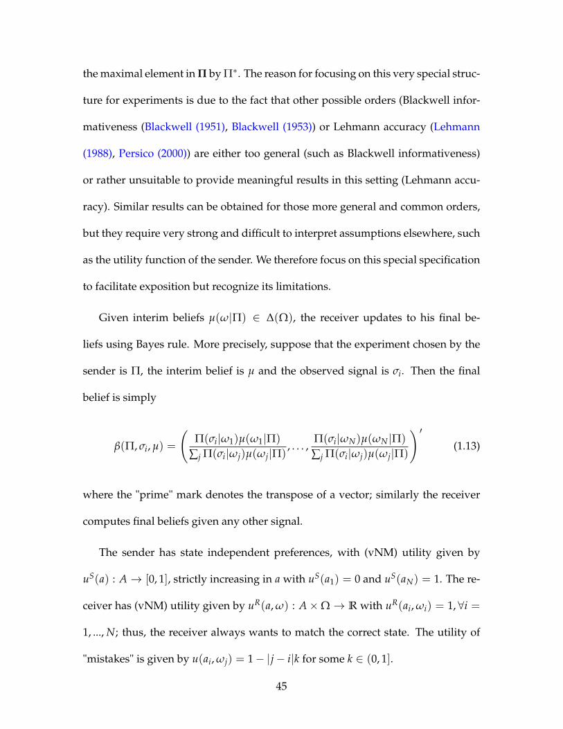
the maximal element in Π by Π∗. The reason for focusing on this very special struc-

ture for experiments is due to the fact that other possible orders (Blackwell infor-

mativeness (Blackwell (1951), Blackwell (1953)) or Lehmann accuracy (Lehmann

(1988), Persico (2000)) are either too general (such as Blackwell informativeness)

or rather unsuitable to provide meaningful results in this setting (Lehmann accu-

racy). Similar results can be obtained for those more general and common orders,

but they require very strong and difficult to interpret assumptions elsewhere, such

as the utility function of the sender. We therefore focus on this special specification

to facilitate exposition but recognize its limitations.

Given interim beliefs µ(ω|Π) ∈ ∆(Ω), the receiver updates to his final be-

liefs using Bayes rule. More precisely, suppose that the experiment chosen by the

sender is Π, the interim belief is µ and the observed signal is σi. Then the final

belief is simply

β(Π, σi, µ) =

(Π(σi|ω1)µ(ω1|Π)

∑j Π(σi|ωj)µ(ωj|Π), . . . ,

Π(σi|ωN)µ(ωN|Π)

∑j Π(σi|ωj)µ(ωj|Π)

) ′(1.13)

where the "prime" mark denotes the transpose of a vector; similarly the receiver

computes final beliefs given any other signal.

The sender has state independent preferences, with (vNM) utility given by

uS(a) : A→ [0, 1], strictly increasing in a with uS(a1) = 0 and uS(aN) = 1. The re-

ceiver has (vNM) utility given by uR(a, ω) : A×Ω → R with uR(ai, ωi) = 1, ∀i =

1, ..., N; thus, the receiver always wants to match the correct state. The utility of

"mistakes" is given by u(ai, ωj) = 1− |j− i|k for some k ∈ (0, 1].

45

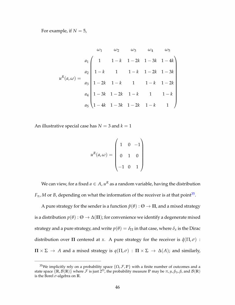
For example, if N = 5,

uR(a, ω) =

ω1 ω2 ω3 ω4 ω5

a1 1 1− k 1− 2k 1− 3k 1− 4k

a2 1− k 1 1− k 1− 2k 1− 3k

a3 1− 2k 1− k 1 1− k 1− 2k

a4 1− 3k 1− 2k 1− k 1 1− k

a5 1− 4k 1− 3k 1− 2k 1− k 1

An illustrative special case has N = 3 and k = 1

uR(a, ω) =

1 0 −1

0 1 0

−1 0 1

We can view, for a fixed a ∈ A, uR as a random variable, having the distribution

Fπ, M or B, depending on what the information of the receiver is at that point35.

A pure strategy for the sender is a function p(θ) : Θ→ Π, and a mixed strategy

is a distribution p(θ) : Θ→ ∆(Π); for convenience we identify a degenerate mixed

strategy and a pure strategy, and write p(θ) = δΠ in that case, where δx is the Dirac

distribution over Π centered at x. A pure strategy for the receiver is q(Π, σ) :

Π × Σ → A and a mixed strategy is q(Π, σ) : Π × Σ → ∆(A); and similarly,

35We implicitly rely on a probability space Ω,F , P with a finite number of outcomes and astate space R,B(R) where F is just 2Ω, the probability measure P may be π, µ, βS, β, and B(R)is the Borel σ-algebra on R.

46

denote by q(Π, σ) = δa a degenerate mixed (i.e. pure) strategy of playing action a.

Let i > j, and suppose that the family ξ satisfies the MLRP. We can make the

following immediate

Observation 1. The family of posteriors of the sender, βS(ω|θ), are ranked according to

the FOSD order (Milgrom (1981)). In other words, for ωi > ωj, and θi > θj,

ξ(θi|ωi)

ξ(θi|ωj)≥

ξ(θj|ωi)

ξ(θj|ωj)⇒ BS(ω|θi) FOSD BS(ω|θj) (1.14)

In other words, a higher observed signal type for the sender is always "good

news" in the sense of FOSD.

From now on we will focus only on pure strategies, for both sides of the game,

to simplify the analysis; again, suppose that the receiver breaks any ties in favor

of the higher action, so that the sender’s expected utility function is upper-semi-

continuous. This assumption is rather less than innocuous, since one might lose

the existence of equilibrium, in addition to narrowing down the scope of possi-

bilities. Nevertheless we are forced to make it to solve the game, as well as to

extend the results clearly; from now on, write p(θ) = Π, for some Π ∈ Π, and

q(Π, σ) = a, for a ∈ A. We can extend the definition of fully nontrivial, partially

nontrivial and pooling equilibria in a straightforward way.

Suppose that the receiver holds final beliefs β(ω|Π, σ, µ). The problem facing

him at that point is

maxa∈A

∑j

uR(a, ωj)β(ωj|Π, σ, µ) (1.15)

47

which is clearly just maximizing the expected value of the random variable uR by

choice of a. Let a∗(Π, σ, µ) or, equivalently, a∗(β)36 denote the solution. Suppose

that in the case a tie, the receiver chooses the higher action; this assumption along

with the specification of preferences yields the observation that the receiver’s best

response is always a pure strategy. The following lemma, the proof of which is the

appendix, is not necessary for out analysis, but interesting in it’s own right, given

that the preferences of the receiver aren’t just to take higher actions - they are to

take the correct action:

Lemma 1.4.1. The function β 7→ a∗(β) is weakly increasing in the following sense: if

B ′ FOSD B, then either a∗(β ′) A a∗(β) or a∗(β ′) = a∗(β).

We can similarly define a function that gives each type’s expected payoff for a

fixed interim belief µ as follows:

v(Π, θi, µ) , Eω

(Eσ(uS(a∗(β(Π, σ, µ))))|θi

)= ∑

kβS(ωK|θi)∑

juS(a∗(β(Π, σj, µ)))Π(σj|ωk)

(1.16)

Optimality requires that for each θi,

Π ∈ arg maxΠ∈Π

v(Π, θi, µ(Π)) (1.17)

We can make several observations about v. First, for a fixed Π, and i, if M ′ FOSD

M, then v(Π, θi, µ ′) ≥ v(Π, θi, µ); this follows from Observation 1 and Lemma 4.1.

In other words, ceteris paribus, a more optimistic interim belief is unequivocally

36Hopefully the abuse of notation does not create confusion.

48

beneficial for the sender. Second, for a fixed Π and µ, i > l, then v(Π, θi, µ) ≥

v(Π, θl, µ).

We have so far omitted a discussion of the role of the interim beliefs of the

receiver about the type of sender: ν = ν(θ|Π) ∈ ∆(Θ). It plays the same role,

specifying the equilibrium beliefs of the receiver, according to the strategies of the

different types of sender.

The first basic observation that we can make is about existence of fully pool-

ing37 equilibria; while we make a strong assumption about π and ξ in doing so,

this is just to give a sufficient condition that is both simple, and works across dif-

ferent other parameters:

Proposition 19. Suppose that π and ξ are such that for all ρ, βS(ω1|θ1) ≥ ρ(N−1)β(ωN |θ1)1−ρ .

Then there exist fully pooling equilibria.

Proof. As usual, we support such equilibria by extremely "pessimistic" beliefs.

Suppose that p(θi) = Πρ for all i, for some Πρ. Thus, on the equilibrium path

µ(Πρ) = π and suppose that in case of a deviation the receiver believes that it

came from the lowest type: µ(Πρ ′′) = β(ω|θ1), ρ ′′ 6= ρ ′. Then, given the restric-

tion in the statement of the proposition, the receiver will find it optimal to take the

lowest action, a1, regardless of the signal. For all types of the sender this entails a

utility of zero, and thus, this deviation will not be profitable.

37We focus on fully pooling equilibria, namely those where all types of sender use the same purestrategy. There may exist others, with some pooling and some separation, but for the purposes ofapplying criterion BPM, there is no difference whether an equilibrium involves separation by sometypes or not.

49

While we don’t know what the function σ 7→ a∗(σ) looks like in general, with-

out still further assumptions, we can make the following useful definition:

Definition 6 ("Kind" of an equilibrium). Let e ′ and e ′′ be two equilibria. We say that

these equilibria are of the same kind if in each equilibrium, on and off the equilibrium path,

the mapping σ 7→ a∗(σ) between the realized signal in experiments that are chosen with

any probability (including zero) is the same.

This definition generalizes the nomenclature for the kinds of equilibria encoun-

tered in the simple model and adapts it to a case with many actions and many

states. We also assume that different equilibria of the same kind coexist. Since the

simplest model discussed in the beginning is a special case of this one, we know

that equilibria can, in fact coexist.

Instead of fully characterizing all equilibria, and then applying a refinement,

we now focus just on pooling equilibria, and show that BPM operates in a similar

and attractive way in a setting with a non-dichotomous state. A full characteriza-

tion is available, but is not any more enlightening than in the case with two states.

Thus, let us simply suppose that ξ and Π are such that there is a continuum of FNT

equilibria38.

Before we state the general version of the main theorem, we need an additional

definition.

Definition 7 ("Rank" of an action). Let e be a fully pooling equilibrium. The rank of an

38It is possible to give explicit conditions that would guarantee this, but assuming those condi-tions would be equivalent to assuming this, and not elucidate anything in addition, so we are notexplicit about them.

50

action, denoted by n(a) is given by the following expression: n(a) , cardσ|a∗(σ) = a

on the equilibrium path.

In other words, the rank of an action is the number of signals that lead to that

action on the equilibrium path. In particular, in a fully nontrivial equilibrium the

rank of each action is equal to unity. We have the following immediate observation,

the proof of which stems from comparing the definitions of kind and rank, and

which we thus omit - if two equilibria are of the same kind, then all receiver actions

in those equilibria have the same rank, but the converse is not necessarily true.

Theorem 1.4.2. Suppose that e ′ and e ′′ are two fully pooling equilibria of the same kind,

with pooling on Πρ ′ and Πρ, respectively; suppose also ρ ′ > ρ. Suppose that the receiver

takes at least two different actions on the equilibrium path and that the maximum rank

of any action is bounded39 above by N3 . The unique (among equilibria of the same kind)

equilibrium that survives criterion BPM is the equilibrium where the pooling is on the

most informative experiment, Πρ ′ .

The proof of the theorem is in the appendix; it goes along the same lines as

the two-state case - computing the relevant utilities. Note also that this defini-

tion generalizes the selection among equilibria encountered in the simple model;

there, too, criterion BPM was used to select among the different kinds of equilib-

ria. Notably, however, in the simple model criterion BPM could not select between

some equilibria simply because they did not coexist for the same parameters, and

39We can give a weaker bound, and in fact, it will be apparent in the proof, but this is a conve-nient uniform, albeit stronger bound that also works.

51

thus the question of selection among them was meaningless. While this can also

happen in a more general setting for some specification of π, ξ and Π, if different

kinds of equilibria do coexist, we expect criterion BPM to operate in the same way

and select the equilibria with the most revelation of information. A proof of this

statement would rely on a particular specification, and lacking one, we do not give

it.

We conclude this section by noting that the results of the model in this section

are rather similar to the simpler model, as was expected. Not only does criterion

BPM apply in a setting with more than two states, but it also operates in a manner

that is analogous to that of the setting with a binary state.

1.5 Concluding Remarks

We present a relatively simple and straightforward model of communication be-

tween an imperfectly informed sender who is trying to persuade a receiver to take

a certain action. The model differs somewhat from existing work, yet is tractable

enough to derive similar (and in some cases, stronger) results. We work with a ba-

sic example using a particular specification of preferences and available informa-

tion structures, that allows us to make reasonably strong predictions. We further

refine the predictions using a novel yet intuitive refinement concept.

There are a number of directions in which this model can be extended in a

fruitful way. For example, the sets of available experiments may vary with the

state. This introduces an additional consideration for the receiver - if he doesn’t

52

see a certain signal, does that mean that the sender chose not to send it, or is it

because it is not available? A similar restriction can apply to the types of sender;

in the general model these restrictions would be manifested by conditions on ξ

and Π.

As a final note, and another way forward for future research, Hedlund (2017)

shows that in his setting with N ≥ 2 types, focusing on only two signals actually

does involve some loss of generality; we appeal to the work of Taneva (2016) to

argue that in general, one can restrict attention to "direct" experiments; however,

it remains unclear if the restriction to symmetric experiments, and ones that are

ranked by the "more precise than" criterion leads to any loss of generality.

Alonso and Camara (2016b) show that if a fully revealing information struc-

ture is available, then an uninformed sender (i.e. before, or without observing a

private signal, in this paper, θ) can replicate any distribution of payoffs that can

be achieved by an informed sender, and therefore, in a sense, private information

is not useful in that setting. Their result does not apply to this model; this is to

say that in realistic settings the sender will, in general, be able to manipulate the

actions of the receiver based on what she knows.

Thus, while the assumption of the existence of a perfectly revealing experi-

ment allows for characterization of equilibria, it also generates very specific re-

sults. More generally, it seems to be emerging from this and similar models that

the mere presence or availability of a fully revealing experiment is one of the key

features (among others, as discussed above) that drive results. In recent work on

multi-sender persuasion an interestingly similar insight has emerged - the capabil-

53

ity of one player to unilaterally mimic a particular distribution of signals (which

can be thought of as an analogue to a fully revealing experiment in a single-sender

framework) has become a key condition.

54

Appendix A: Proofs

Proof of Proposition 11. First, it is immediate that SEP is a BPM equilibrium, since

there are no out-of-equilibrium beliefs to consider, and thus criterion BPM is triv-

ially satisfied. The reason that PNT-LL(aH) and PNT-HH(aH) survive criterion

BPM (note also that from proposition 10 we know that they coexist, so it is mean-

ingful to talk about choosing between them) is that deviations from those equi-

libria do not yield a strictly higher payoff for either type. The computation that

eliminates FNT-L and PNT-LH(aL) goes as follows: Take any pooling equilibrium

where both both types choose the experiment ΠL and the receiver takes different

actions on the equilibrium path. In that equilibrium, u∗(θH) =

v(ΠL, π, θH) = ρL

[P(ωH|θH)1β(ΠL,σH ,π)≥ 1

2+ P(ωL|θH)1β(ΠL,σL,π)≥ 1

2

]+

+(1− ρL)[P(ωH|θH)1β(ΠL,σL,π)≥ 1

2+ P(ωL|θH)1β(ΠL,σH ,π)≥ 1

2

](1.18)

and u∗(θL) =

v(ΠL, π, θL) = ρL

[P(ωH|θL)1β(ΠL,σH ,π)≥ 1

2+ P(ωL|θL)1β(ΠL,σL,π)≥ 1

2

]+

+(1− ρL)[P(ωH|θL)1β(ΠL,σL,π)≥ 1

2+ P(ωL|θL)1β(ΠL,σH ,π)≥ 1

2

] (1.19)

55

Fix a µ and consider the utility of deviating to ΠH for both types:

v(ΠH, µ, θH)− u∗(θH) = ρH

[P(ωH|θH)1µ|β(Πi,σH ,µ)≥ 1

2+ P(ωL|θH)1|µ|β(Πi,σL,µ)≥ 1

2

]+

+(1− ρH)[P(ωH|θH)1µ|β(Πi,σL,µ)≥ 1

2+ P(ωL|θH)1µ|β(Πi,σH ,µ)≥ 1

2

]−

−ρL

[P(ωH|θH)1β(ΠL,σH ,π)≥ 1

2+ P(ωL|θH)1β(ΠL,σL,π)≥ 1

2

]+

+(1− ρL)[P(ωH|θH)1β(ΠL,σL,π)≥ 1

2+ P(ωL|θH)1β(ΠL,σH ,π)≥ 1

2

]=

= (P(ωH|θH)) [ρH1µ|β(Πi,σH ,µ)≥ 12− ρL1β(ΠL,σH ,π)≥ 1

2+ (1− ρH)1µ|β(Πi,σL,µ)≥ 1

2−

−(1− ρL)1β(ΠL,σL,π)≥ 12] + (P(ωL|θH))[ρH1|µ|β(Πi,σL,µ)≥ 1

2− ρL1β(ΠL,σL,π)≥ 1

2+

+(1− ρH)1µ|β(Πi,σH ,µ)≥ 12− (1− ρL)1β(ΠL,σH ,π)≥ 1

2]

(1.20)

Now let µ solveρHµ

ρHµ+(1−ρH)(1−µ)= 1

2 , (i.e. µ = 1− ρH) and let µ solve ρLµρLµ+(1−ρL)(1−µ)

=

12 (i.e. µ = 1 − ρL) and note that since ρH > ρL, µ < µ. Also let †µ solve

(1−ρL)†µ(1−ρL†µ+ρL(1−†µ))

= 12 (i.e. †µ = ρL ) and µ† = (1−ρH)µ†

(1−ρH)µ†+ρH(1−µ†) =12 (i.e. µ† = ρH

) and note that †µ < µ†. As before, we focus on nontrivial equilibria (so that we

can disregard the terms that involve observing the low signal/action). Now we

56

can directly compute

v(ΠH, θH, µ)− u∗(θH)− (v(ΠH, θL, µ)− u∗(θL)) =

= [P(ωH|θH)−P(ωH|θL)][ρH1µ|β(Πi,σH ,µ)≥ 1

2− ρL1β(ΠL,σH ,π)≥ 1

2

]+

+[P(ωL|θH)−P(ωL|θL)][(1− ρH)1µ|β(Πi,σH ,µ)≥ 1

2− (1− ρL)1β(ΠL,σH ,π)≥ 1

2

]=

=

u∗(θL)− u∗(θH) < 0, for µ ∈ [0, µ)

2(ρH − ρL)(P(ωHθH)−P(ωH|θL))) > 0 for µ ∈ [µ, †µ)

2ρL[P(ωH|θL)−P(ωH|θH)] + P(ωH|θH)−P(ωH|θL) < 0 for µ ∈ [†µ, 1]

(1.21)

Since the difference is negative for first of the three ranges exhibited above, cri-

terion BPM does not apply there. For the second range of beliefs the difference

is strictly positive, and hence, beliefs that support PNT-LH(aL) are ruled out. As

for the third range, the difference is negative, but beliefs there are such that they

cannot be part of any kind of nontrivial equilibrium at all (cf. the upper bounds

on off-path beliefs for equilibria in Propositions 4 through 9 and note that criterion

BPM restricts beliefs off the equilibrium path) and we are done.

Proof of Lemma 1.4.1. We first state the following common lemma (which is the dis-

crete version of integration by parts) without proof:

Lemma 1.5.1. (Abel’s lemma)

Let aini=1 and bin

i=1 be two sequences of real numbers. Let Ai = ∑ij=1 aj and

57

Bi = ∑ij=1 bj. Then

n

∑i

aibi =n−1

∑i

Ai(bi − bi+1) + Anbn (1.22)

Suppose that B ′(ω) FOSD B(ω) and fix take any a ′, a with a ′ > a. Consider

the following difference:

[∑

ju(a ′, ωj)β ′(ωj)−∑

ju(a, ωj)β ′(ωj)

]−[∑

ju(a ′, ωj)β(ωj)−∑

ju(a, ωj)β(ωj)

]=

=N−1

∑j

(B ′(ωj)− B(ωj)

) [u(a ′, ωj)− u(a, ωj)− u(a ′, ωj+1) + u(a, ωj+1)

](1.23)

where the equality is just applying Abel’s lemma to appropriately defined vari-

ables, and the the fact that B ′(ωk) = ∑ki=1 β ′(ωi) and B(ωk) = ∑k

i=1 β(ωi) are

discrete distribution functions. Given the utilities, it can then be checked by di-

rect computation that the term is the square brackets weakly increasing in ω; this,

combined with the fact that β ′ FOSD β shows that the entire expression is non-

negative. In other words, that the function f (a, β) , Eβu(a, ω) has increasing dif-

ferences in (a, β). The fact that a∗(β ′) A a∗(β) or a∗(β ′) = a∗(β) for β ′ FOSD β

then follows by a standard argument. Namely, the choice set is totally ordered (a

one-dimensional "chain", so that supermodularity trivially holds), the set of beliefs

is a partially ordered set according to FOSD and f has increasing differences (and

so also satisfies the single crossing condition). Thus, a∗(β) is monotone nonde-

creasing in β (Milgrom and Shannon (1994)), and we are done.

Proof of Theorem 1.4.2. We again compute the relevant utilities. In the baseline equi-

58

Now taking the difference between the utilities between different sender types

v(Πρ ′ , µ, θi)− u∗(θi)− v(Πρ ′ , µ, θl) + u∗(θl) =

= ∑k(βS(ωk|θi)− βS(ωk|θl))

[(ρ ′ − ρ))(uS(ak)(n(ak)− 1σk|a∗(σk)=ak+

+ ∑j

(ρ− ρ ′

N − 1


]] (1.29)

Now letting

φ(ρ, ρ ′, ωk) , (ρ ′ − ρ))(uS(ak)(n(ak)− 1σk|a∗(σk)=ak)+

+∑j

(ρ− ρ ′

N − 1


] (1.30)

be the function that gives the expected utility of deviation as a function of the

state and parameters, it can once again be checked directly that φ(ρ, ρ ′, ωk+t) −

φ(ρ, ρ ′, ωk) ≥ 0 for t = 1, 2, ..., N − k. There are six cases to consider (this is also

where the condition n(a) ≤ N3 emerges from):

1. n(ak) = n(ak+t) > 0; in this case the expression φ(ρ, ρ ′, ωk+t)− φ(ρ, ρ ′, ωk)

is positive as long as n(ak) = n(ak+1) ≤ N3 .

2. n(ak) = n(ak+t) = 0; in this case the expression φ(ρ, ρ ′, ωk+t)− φ(ρ, ρ ′, ωk)

is zero.

3. n(ak) > n(ak+t) > 0; in this case the expression φ(ρ, ρ ′, ωk+t)− φ(ρ, ρ ′, ωk)

is positive.

60

4. n(ak+t) > n(ak) > 0; in this case the expression φ(ρ, ρ ′, ωk+t)− φ(ρ, ρ ′, ωk)

is positive.

5. n(ak) > n(ak+t) = 0; in this case the expression φ(ρ, ρ ′, ωk+t)− φ(ρ, ρ ′, ωk)

is positive as long as n(ak) ≤ N2 .

6. n(ak+t) > n(ak) = 0; in this case the expression φ(ρ, ρ ′, ωk+t)− φ(ρ, ρ ′, ωk)

is positive as long as n(ak+t) ≤ N2 .

and thus φ(ρ, ρ ′, ωk) is increasing in ω, and hence by the definition of first-order

stochastic dominance, the entire expression in equation 1.29 is weakly positive and

we are done.

61

Chapter 2

Characterization, Existence and Pareto Optimality in

Insurance Markets with Asymmetric Information with

Endogenous and Asymmetric Disclosures: Revisiting

Rothschild-Stiglitz

This chapter is coauthored with Joseph E. Stiglitz and Jungyoll Yun.

Introduction

Some forty years ago, Rothschild and Stiglitz (1976) characterized equilibrium in

a competitive market with exogenous information asymmetries in which market

participants had full knowledge of insurance purchases. Self-selection constraints

affected individual choices; but unlike the monopoly equilibrium1, no single firm

framed the set of contracts among which individuals chose. There never existed

a pooling equilibrium (in which the two types bought the same policy); if there

existed an equilibrium, it entailed the high risk getting full insurance, and the low

risk individual only getting partial insurance; and under plausible conditions -

1Stiglitz (1977)

62

e.g. if the two types were not too different - a pure strategy equilibrium did not

exist. The paper was unsatisfactory not only in its results (equilibrium seemed to

exist, and often entailed pooling) but on its reliance on a special property, called the

single crossing property, whereby the indifference curve of the high risk individual

could cross that of the low risk individual only once (if at all)2.

Since their work, there has been huge literature applying the model to labor,

capital, and product markets in a variety of contexts, a large number of empiri-

cal applications, and a small literature trying to repair the deficiencies in the un-

derlying framework by formalizing the insurance "game", by changing the infor-

mation/disclosure assumptions, and by changing the equilibrium concept. This

paper takes an approach that differs fundamentally from this earlier literature by

endogenizing the disclosure of information about insurance purchases: each firm

and consumer makes a decision about what information to disclose to whom -

thus information about contract purchases is not only endogenous but potentially

asymmetric. The results were somewhat surprising even to us: (i) asymmetries

in information about insurance purchases, especially associated with out of equi-

librium moves, do indeed turn out to be important; (ii) there always exists an

equilibrium, even when the single crossing property is not satisfied; and (iii) the

equilibrium always entails a pooling contract. Indeed, the unique insurance allo-

cation (an insurance allocation describes the sum of benefits and premia for each

individual) consists of the pooling allocation which maximizes the well-being of

2As innocuous as it might seem, it won’t be satisfied if the high and low risk individuals differin their risk aversion; and with multi-crossings, equilibrium, if it exists, can look markedly differ-ent.

63

the low risk individual (along the zero profit pooling line) plus a supplemental

contract that brings the high risk individual to full insurance (at his own odds).

While the equilibrium allocation is unique, it can be supported by multiple alter-

native information strategies. We begin the analysis by characterizing the set of

Pareto efficient (PE) allocations in the presence of a possibly secret contract. We

then show that the PE allocation which maximizes the well-being of the low risk

individual is the unique equilibrium allocation and can be supported by simple

information disclosure strategies.

While the analysis is complex, it is built upon a number of steps, each of which

itself is relatively simple. As in RS, insurance firms offer insurance contracts, but

now they may or may not decide to reveal information (all or partial) about insur-

ance purchases to other firms. In RS, it was assumed that contracts were exclusive,

e.g. implicitly, that if a firm discovered a purchaser had violated the exclusivity

restriction, the coverage would be cancelled. Here, we consider a broader range

of possible restrictions. Obviously, the enforceability of any conditions imposed is

dependent on information available to the insurance firm. Consumers, too, have

a slightly more complicated life than in RS: they have to decide which policies

to buy, aware of the restrictions in place and the information that the insurance

firm may have to enforce those restrictions. And they also have to decide on what

information to reveal to whom3.

As in RS, a competitive equilibrium is described by a set of insurance contracts,

3We assume that consumers can only reveal information to firms, and not to other consumers.Since the game is one of private values, revealing information to other consumers is moot, andtherefore we disallow it without loss of generality.

64

such that no one can offer an alternative contract or set of contracts and make

money. Here, though, a contract is defined not just by the benefit and the premium,

but also by the restrictions associated with the contract and the firm’s disclosure

policy.

The paper is divided into 12 sections. In the first, we set out the standard in-

surance model. In the second we recall why RS resorted to exclusive contracts. We

explain how the existence of a (non-loss making) secret contract offered at the odds

of the high risk individual (a) upsets the separating equilibrium; (b) implies that

some of the contracts that broke the pooling contract no longer do so; but (c) there

always exist some contracts that nevertheless break the relevant pooling allocation.

Section 3 then shows that if there is a non-disclosed contract (at the odds of the high

risk individual), the Pareto efficient contracts are always of a simple form: pooling

plus supplemental insurance purchased only by high risk individuals. Section 4

then defines the competitive equilibrium. Section 5 shows that regardless of the

strategies, if there is a competitive equilibrium, the allocation must be the Pareto

efficient allocation which maximizes the wellbeing of the low risk individual. Sec-

tion 6 then describes equilibrium strategies for firms and consumers, shows that

the posited strategies support the equilibrium allocation described in the previ-

ous section, and are robust against any deviant contract. Section 7 comments on

several salient properties of the result and its proof, including that it does not re-

quire the single crossing property, but only a much weaker condition. Section 8

and 9 discuss uniqueness of equilibria and show how the equilibrium construct

can be extended, for instance to other disclosure strategies and to multiple types

65

of individuals. Sections 10 and 11 relate our results to earlier literature. In par-

ticular, section 11 considers the standard adverse selection price equilibrium. We

show how our analysis implies that in general a price equilibrium does not exist if

there can exist a (non-loss making) insurance contract the purchase of which is not

disclosed. Section 12 presents some concluding comments.

2.1 The Model

We employ the standard insurance model with adverse selection. An individual

is faced with the risk of an accident with some probability, Pi. Pi depends upon

the type i of the individual. There are two types of individuals - high risk and

low risk - who differ from each other only in the probability of accident. The type

is privately known to the individual, while the portion θ of H-type is common

knowledge. The weighted average probability of accident for an individual is P,

where

P , θPH + (1− θ)PL

An accident involves damages. The cost of repairing the damage in full is d. An

insurance firm pays a part of the repair cost, α ≤ d. The benefit is paid in the event

of accident, whereas the insurer is paid insurance premium β when no accident

occurs4. The price of insurance, q, is defined by βα . (In market equilibrium, the

amount of insurance that an individual can buy may be limited.) The expected

4This has become the standard formulation since RS. In practice, customers pay β the periodbefore the (potential) accident, receiving back α + β in the event the accident occurs, i.e. a netreceipt of α.

66

utility for an individual with a contract (α, β) is

Vi(α, β) = PiU(w− d + α) + (1− Pi)U(w− β) (2.1)

For expository purposes the reader may assume that the Bernoulli utility function

U is quasi-concave and differentiable, with U” < 0 (individuals are risk averse).

Sometimes we refer to an allocation A , (α, β), in which case we can refer to

the expected utility generated by that contract as Vi(A)5. Under the conditions

leading to equation 2.1, an indifference curve for high-risk individual is steeper

than that for low-risk one at any (α, β), generating the so-called the single-crossing

property. As will be shown later in the paper, however, we can allow for more

general preferences, e.g. with a different utility function Ui for each type i6. In

this case, the single crossing property will not be satisfied. The key property of

Vi(α, β) is that the income consumption curve at the insurance price Pi1−Pi

is the full

insurance line7, implying that at full insurance, the slope of the indifference curve

equals the relative probabilities,

∂Vi(α,β)∂β

∂Vi(α,β)∂α

=Pi

1− Pi

so that will full information, equilibrium would entail full insurance for each type

5Similarly, if the individual purchases policies A and B, we can refer to the expected utilitygenerated as Vi(A + B)

6Indeed, we do not even require preferences to satisfy the conditions required for behaviortowards risk to be described by expected utility. We do not even require quasi-concavity.

7That is even if the indifference curve is not quasi concave, after being tangent to a given iso-cline with slope Pi

1−Pi, at full insurance, it never touches the isocline again.

67

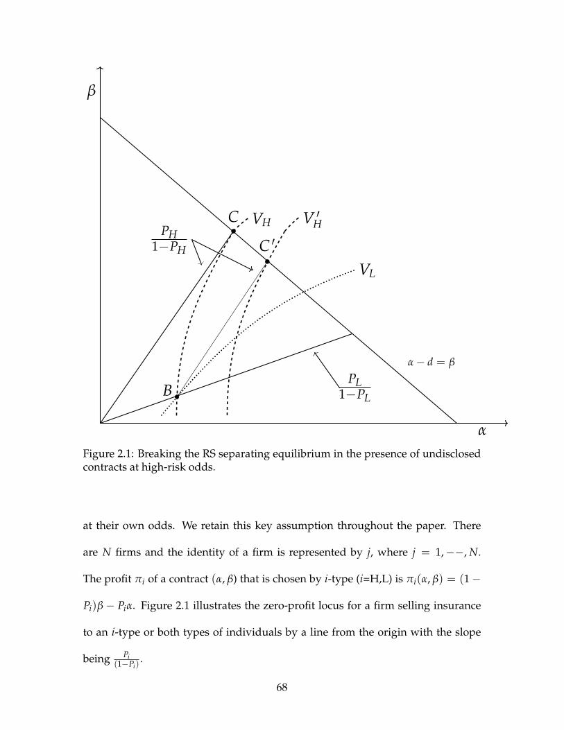
α

β

α− d = β

PH1−PH

VL

VH V ′H

B

C

C ′

PL1−PL

Figure 2.1: Breaking the RS separating equilibrium in the presence of undisclosedcontracts at high-risk odds.

at their own odds. We retain this key assumption throughout the paper. There

are N firms and the identity of a firm is represented by j, where j = 1,−−, N.

The profit πi of a contract (α, β) that is chosen by i-type (i=H,L) is πi(α, β) = (1−

Pi)β− Piα. Figure 2.1 illustrates the zero-profit locus for a firm selling insurance

to an i-type or both types of individuals by a line from the origin with the slope

being Pi(1−Pi)

.

68

2.2 Rothschild-Stiglitz with Secret Contracts

Central to the analysis of RS was the assumption that there was sufficient informa-

tion to enforce exclusivity; the individual could not buy insurance from more than

one firm. As RS realized, once we introduce into the RS analysis unobservable

contracts in addition to the observable ones, the whole RS framework collapses.

Exclusivity cannot be enforced. In this section, we review why they assumed ex-

clusivity; we assume that undisclosed contracts can and will be offered if they at

least break-even. In particular, we know that a price contract (where the individ-

ual can buy as much of the given insurance at the given price) with a price PH1−PH

will at least break even: if it is bought by any low risk individual, it makes a profit.

Breaking a Separating Equilibrium

When there is secret supplemental insurance, the implicit self-selection constraints

change, because whether an individual prefers contract A rather than B depends

on whether an individual prefers A plus the optimally chosen secret contract to

B plus the optimally chosen secret contract. Thus, in figure 2.1, the high risk in-

dividual prefers the contract which puts him on the highest indifference curve at

slope PH1−PH

. Consider the standard RS equilibrium separating contracts, C and B.

C is the full insurance contract for the high risk individual assuming he was not

subsidized or taxed and B is the contract on the low risk individual’s break-even

curve that just separates, i.e. is not purchased by the high risk individual8. B, C

8In RS, the pair of contracts B, C constitutes the equilibrium so long as B is preferred to thecontract on the pooling line which is most preferred by the low risk individual. If this is not true,

69

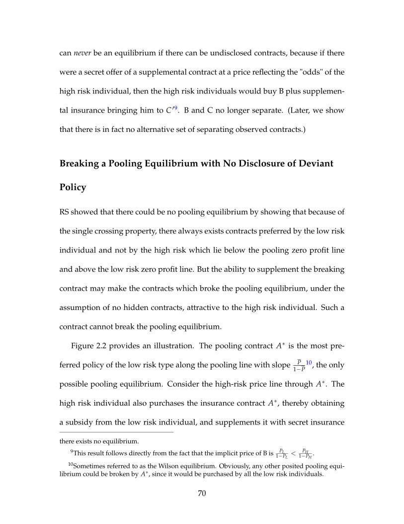
can never be an equilibrium if there can be undisclosed contracts, because if there

were a secret offer of a supplemental contract at a price reflecting the "odds" of the

high risk individual, then the high risk individuals would buy B plus supplemen-

tal insurance bringing him to C ′9. B and C no longer separate. (Later, we show

that there is in fact no alternative set of separating observed contracts.)

Breaking a Pooling Equilibrium with No Disclosure of Deviant

Policy

RS showed that there could be no pooling equilibrium by showing that because of

the single crossing property, there always exists contracts preferred by the low risk

individual and not by the high risk which lie below the pooling zero profit line

and above the low risk zero profit line. But the ability to supplement the breaking

contract may make the contracts which broke the pooling equilibrium, under the

assumption of no hidden contracts, attractive to the high risk individual. Such a

contract cannot break the pooling equilibrium.

Figure 2.2 provides an illustration. The pooling contract A∗ is the most pre-

ferred policy of the low risk type along the pooling line with slope P1−P

10, the only

possible pooling equilibrium. Consider the high-risk price line through A∗. The

high risk individual also purchases the insurance contract A∗, thereby obtaining

a subsidy from the low risk individual, and supplements it with secret insurance

there exists no equilibrium.9This result follows directly from the fact that the implicit price of B is PL

1−PL< PH

1−PH.

10Sometimes referred to as the Wilson equilibrium. Obviously, any other posited pooling equi-librium could be broken by A∗, since it would be purchased by all the low risk individuals.

70

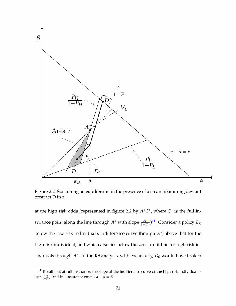
α

β

PL1−PL

A∗

α

α− d = β

VL

PL1−PL

Area z

D

C∗P

1−PPH1−PH

αD

D ′

D0

Figure 2.2: Sustaining an equilibrium in the presence of a cream-skimming deviantcontract D in z.

at the high risk odds (represented in figure 2.2 by A∗C∗, where C∗ is the full in-

surance point along the line through A∗ with slope PH1−PH

)11. Consider a policy D0

below the low risk individual’s indifference curve through A∗, above that for the

high risk individual, and which also lies below the zero profit line for high risk in-

dividuals through A∗. In the RS analysis, with exclusivity, D0 would have broken

11Recall that at full insurance, the slope of the indifference curve of the high risk individual isjust PH

1−PH, and full insurance entails α− d = β

71

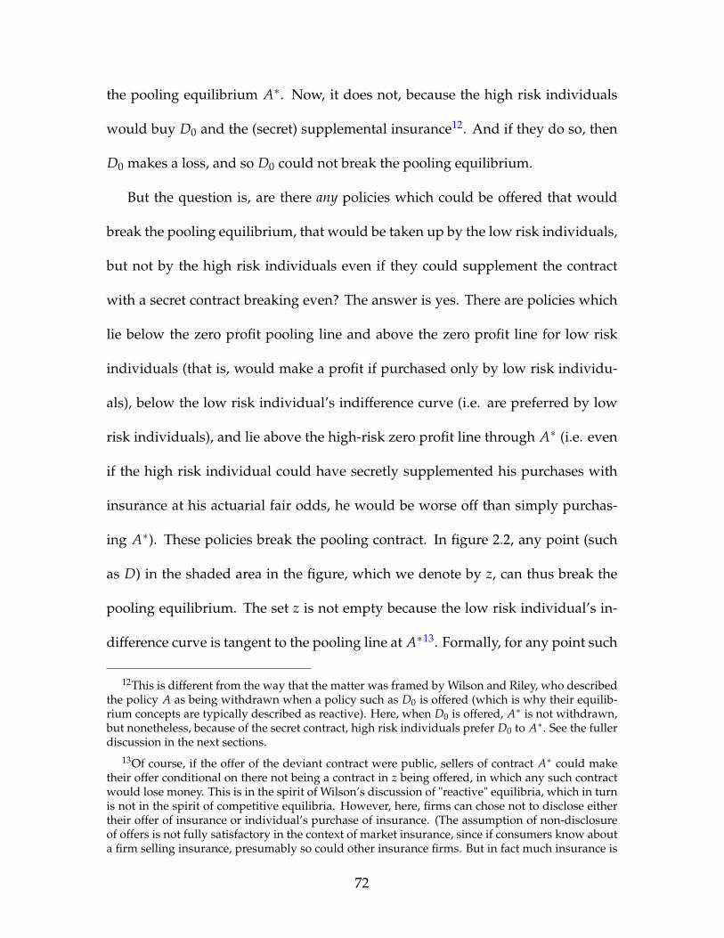
the pooling equilibrium A∗. Now, it does not, because the high risk individuals

would buy D0 and the (secret) supplemental insurance12. And if they do so, then

D0 makes a loss, and so D0 could not break the pooling equilibrium.

But the question is, are there any policies which could be offered that would

break the pooling equilibrium, that would be taken up by the low risk individuals,

but not by the high risk individuals even if they could supplement the contract

with a secret contract breaking even? The answer is yes. There are policies which

lie below the zero profit pooling line and above the zero profit line for low risk

individuals (that is, would make a profit if purchased only by low risk individu-

als), below the low risk individual’s indifference curve (i.e. are preferred by low

risk individuals), and lie above the high-risk zero profit line through A∗ (i.e. even

if the high risk individual could have secretly supplemented his purchases with

insurance at his actuarial fair odds, he would be worse off than simply purchas-

ing A∗). These policies break the pooling contract. In figure 2.2, any point (such

as D) in the shaded area in the figure, which we denote by z, can thus break the

pooling equilibrium. The set z is not empty because the low risk individual’s in-

difference curve is tangent to the pooling line at A∗13. Formally, for any point such

12This is different from the way that the matter was framed by Wilson and Riley, who describedthe policy A as being withdrawn when a policy such as D0 is offered (which is why their equilib-rium concepts are typically described as reactive). Here, when D0 is offered, A∗ is not withdrawn,but nonetheless, because of the secret contract, high risk individuals prefer D0 to A∗. See the fullerdiscussion in the next sections.

13Of course, if the offer of the deviant contract were public, sellers of contract A∗ could maketheir offer conditional on there not being a contract in z being offered, in which any such contractwould lose money. This is in the spirit of Wilson’s discussion of "reactive" equilibria, which in turnis not in the spirit of competitive equilibria. However, here, firms can chose not to disclose eithertheir offer of insurance or individual’s purchase of insurance. (The assumption of non-disclosureof offers is not fully satisfactory in the context of market insurance, since if consumers know abouta firm selling insurance, presumably so could other insurance firms. But in fact much insurance is

72

as D, VL(D) > VL(A∗), while VH(D + SH) > VH(A∗)14. We collect the results

together in

Proposition 20. i) The RS separating contracts do not constitute an equilibrium, if

firms can offer non-loss making undisclosed contracts.

ii) The pooling equilibrium may always be "broken" if there exists undisclosed supple-

mental insurance and if a deviant firm can choose to keep his offers secret.

iii) Some of the contracts that broke the pooling equilibrium in the standard RS equilib-

rium with exclusivity no longer do so.

The remaining sections focus on the core issue of an endogenous information

structure, with the simultaneous determination of contract offers of firms and with

contract purchases and information disclosure by individual customers.

2.3 Pareto Efficiency with Undisclosed Contracts

In this section, we consider the set of efficient insurance allocations under the

premise that there exists a secret (undisclosed) contract being offered at the price

PH1−PH

. We can think of this as a "constrained P.E." allocation-where the constraint

is that the government cannot proscribe the secret provision of insurance, unlike

the PE allocations associated with the RS model, where government could restrain

non-market insurance (see Arnott and Stiglitz (1991b)), often implicit and not formal, and whethersuch insurance is available to any individual let alone taken up by him may not be known.

14The notation D + SH refers to the (α, β) associated with the purchase of D plus the optimizedvalue of secret insurance along the price line associated with the high risk individual. Given ourassumptions about preferences, we know this brings the high risk individual to full insurance.

73

such provision15. The difficulties in defining Pareto efficiency in settings of in-

complete information are not new16; we use the following ex-interim variant of

constrained Pareto efficiency17:

Definition 8. An allocation E is constrained Pareto-efficient if the government cannot

force disclosure and there does not exist another feasible allocation (i.e. one which at least

breaks even), and leaves each type of consumer as well off and at least one type strictly

better off.

For simplicity of exposition, in this section we that the conditions leading to

equation 2.1 is satisfied. We now establish two general properties that a PE alloca-

tion must satisfy:

Lemma 2.3.1. Every Pareto efficient allocation must be a separating allocation (i.e. one

where the two types of individuals get different allocations), except possibly for the point

along the pooling line providing full insurance.

Any feasible (i.e. making at least zero profit for the firms) pooling allocation

must lie on the pooling line. At any point other than full insurance, the utility of

the high risk individual will be improved by a pair of allocations (A∗ and C∗ in

figure 2.3, for example), that along the pooling line and that bringing the high risk

individual to full insurance from there.

15The analysis of PE allocations in the RS model is in Stiglitz (2009). The terminology may beconfusing. It focuses on the constraints imposed on the government - that it cannot restrict thesecret sale of insurance. From the perspective of the market, of course, it is an "unconstrained"equilibrium - firms do not face the constraint of disclosing.

16See Holmstrom and Myerson (1981).17See also Greenwald and Stiglitz (1986).

74

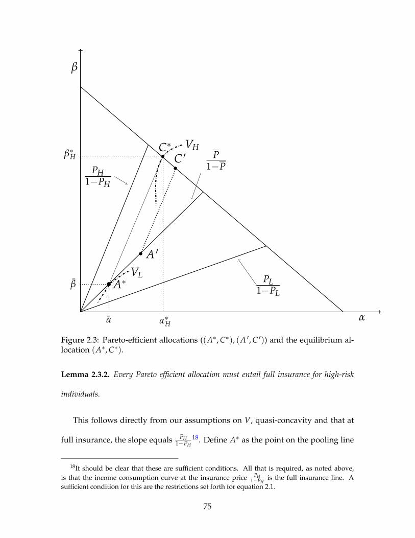
α

β

A∗

A ′

C∗C ′

α α∗H

β

β∗H

VL

VHP

1−PPH1−PH

PL1−PL

Figure 2.3: Pareto-efficient allocations ((A∗, C∗), (A ′, C ′)) and the equilibrium al-location (A∗, C∗).

Lemma 2.3.2. Every Pareto efficient allocation must entail full insurance for high-risk

individuals.

This follows directly from our assumptions on V, quasi-concavity and that at

full insurance, the slope equals PH1−PH

18. Define A∗ as the point on the pooling line

18It should be clear that these are sufficient conditions. All that is required, as noted above,is that the income consumption curve at the insurance price PH

1−PHis the full insurance line. A

sufficient condition for this are the restrictions set forth for equation 2.1.

75

most preferred by the low risk individual, or, more formally, as an allocation (α, β)

such that

α = arg maxα

VL(α,P

1− Pα) and β =

P1− P

α (2.2)

Also, define C∗ as a full-insurance point along the line through A∗ with slope

PH1−PH

, which can be represented as an allocation (α∗H, β∗H) such that

α∗H + β∗H = d, and β∗H − β =PH

1− PH(α∗H − α) (2.3)

Consider contract pairs (A ′, C ′) in figure 2.3 where A ′ lies along the pooling line

and C ′ is the full insurance point along the line through A ′ with slope PH1−PH

, or

where A ′ , (α ′, β′) and C ′ , (α ′H, β ′H) such that

β′=

P1− P

α ′ (2.4)

α ′H + β ′H = d, and β ′H − β′=

PH

1− PH(α ′H − α ′) (2.5)

All such pairs are feasible outcomes. Then for an allocation (A ′, C ′) such that

α ′ < α, an increase in insurance improves the utility of both the high and low

risk individuals, so such allocations cannot be PE. Consider now a contract pair

(A ′, C ′) such that α ′ > α as in figure 2.3. Given C ′ and the existence of secret

contract, is there an alternative feasible allocation preferred by low risk individ-

uals? Any contract purchases just by low risk individuals must lie on or above

76

the line through A ′ with slope PL1−PL

, because otherwise it is not feasible; and on or

above the line through A ′ with slope PH1−PH

, because otherwise it would be chosen

by both the high risk and low risk individual. The only contract satisfying these

two conditions is A ′. On the other hand, any feasible contract purchased by both

types must lie along the pooling line. Along the pooling line, any allocation that

makes the low risk individual better off (by moving towards A∗) makes the high

risk individual worse off. Quasi-concavity of the indifference curves ensures that

the low risk individual’s indifference curve through A ′ has a slope that is steeper

than PL1−PL

. Hence, there exists no Pareto improvement over A ′, C ′. We have thus

fully characterized the set of Pareto efficient allocations.

Proposition 21. The set of PE allocations are those generated by an allocation (α ′, β′)

(defined by equation 2.4) along the pooling line, such that α ′ ≥ α and α ′ + β′ ≤ d, for the

low risk individual; and by an allocation (α ′H, β ′H) (defined by equations 2.4 and 2.5) for

the high risk individual.

2.4 Definition of Market Equilibrium

In this section, we define the market equilibrium.

77

Contract Offers by Firms and Optimal Responses by Consumers

Firms move first, making a set of contract offers19. A contract Ck(= αk, βk, Rk, Dk)

offered by a firm k is represented by a benefit αk, if the accident occurs, a premium

βk, if it does not, a set Rk of restrictions that have to be met for the purchase of

(αk, βk), and a rule Dk of disclosing information at the firm’s disposal, such as

about (αk, βk) sold to individual i. The restrictions Rk, to be relevant, must be

based on observables, i.e. what is revealed to the insurance firm k either by the

insured i or by other insurance firms; and we assume that they relate only to the

purchases of insurance by the insured; they may entail, for instance, a minimum

or maximum amount of insurance obtained from others. The exclusivity provision

of RS is an example of a restriction, but there are obviously many potential others.

Two simple disclosure rules would be to disclose the purchase to every other

firm, or to disclose the purchase to no firm. The equilibrium disclosure rules to

be described below will turn out to be somewhat more complex than (and loosely

speaking, "in between") these simple rules, but still relatively simple.

Following this, households look at the set of contracts on offer (including the

restrictions and disclosure policies) and choose the set of contracts that maximizes

their expected utility, given the contract constraints.

Consumers also have an information revelation strategy, e.g. what informa-

tion (about their purchases) to disclose to whom, taking into consideration dis-

closure policies and contract offers firms announce. In the central model of this

19The firm knows nothing about the individual, other than information about contract pur-chases. The firm may make inferences about the individual based on the information it has abouthis purchases.

78

paper, the individual simply reveals the quantity of pooling insurance purchased

to those firms from whom he has purchased a pooling contract. In an alternative

formulation described briefly in appendix C, he also tells the price at which he has

purchased insurance.

There is a third period which just entails the "working out" of the consequences

of the first two-no new action is taken. The third period takes place in two stages.

In the first, firms disclose information according the disclosure rules they announced.

In the second, each firm checks to see whether any contract restriction is violated,

and if it is, that policy is cancelled. Actually, life is easier than just described, since

consumers who always respond optimally to any set of contracts offered by firms

know that if they violate contract provisions, policies will be cancelled; and in this

model, there is no strategic value of buying policies which will be cancelled20.

Information Disclosure

As we noted, both consumers and firms disclose information on the contracts they

have purchased and sold. We assume that both can withhold information from

others21. The firm or the consumer can disclose just the amount of insurance (α)

or the price (β). Also, as a means of partial revelation of information, a firm might

20This is not a repeated game. Consumers are engaging in a "rational expectations best responsestrategy," which includes identifying which deceptions are caught out, and since such policies arecancelled, not undertaking them.

21We assume that the consumers cannot lie; a consumer or his insurer cannot "reveal" that hepurchased insurance from a firm when no such purchase happened. More succinctly, they tell thetruth, nothing but the truth, but not necessarily the whole truth. In other words, purchased contracts are"hard evidence" that can be revealed if it is available, but cannot be fabricated. We do not analyzethe game where firms are free to engage in strategic disinformation. We do allow a contract to beshown with redacted information (the truth, but not the whole truth.)

79

engage in what we call contract manipulation (or CM for brevity) - dividing its

sales to an individual into multiple policies. This would allow a consumer to dis-

close to others one policy, but to hide the full extent of his insurance purchases22.

As will be shown below, however, no firm sells an individual multiple contracts in

equilibrium, so that no CM occurs in equilibrium.

Suppressing i for notational simplicity, we denote by Ωck and Ω f

k the informa-

tion revealed to firm k by consumer i and by the other firms, respectively. The

information disclosure rule Dk of a contract specifies what information about in-

dividual i firm k reveals to firm j. We assume that the information revealed is a

subset of the information Ωck that the firm has on individual i obtained from indi-

vidual i and the information about its own sale (αk, βk) to the individual. Similarly,

the decision as to whom to disclose is based upon Ωck, (αk, βk). The disclosure

rule of firm k can thus be represented by Dk(Ωck; (αk, βk))

2324. Firms can engage

in discriminatory revelation, revealing information to some firms not revealed to

others, thus creating an asymmetry of information about the insurance coverage of

any individual. If there is discriminatory disclosure, the discrimination has to be

based on some information Ωck previously disclosed by the insured to the firm25.

22This will be one of the main ways in which high-risk types can try to deceive the firms, beinga key element in all information economics models - one type will want to pretend to be the othertype.

23Note that, as contrasted with Jaynes (1978) and Hellwig (1988), the disclosure rule of a firm isnot conditional upon contract offers made by other firms.

24In a slightly more general specification of the game, firms can disclose information that isrevealed to them by other firms. In this case, the third stage of the game has to be extended, tohave a series of rounds of disclosure, i.e. as each firm receives information from other firms (basedon their announced disclosure rule), it discloses some or all of what has been disclosed to it.

25We do not consider random disclosures.

80

Equilibrium

Our equilibrium definition is a straightforward generalization of that of RS, where

a set of contracts was an equilibrium if there did not exist another contract (or

set of contracts) which could be introduced, be purchased by someone, and make

a profit (or at least break even.) Here, contracts are defined by the quadruplet

α, β, R, D. We denote the set of contract offers of firm k by strategy Sk.

Definition 9 (Equilibrium). An equilibrium is a strategy S∗k for each firm k, such that,

given the set S∗j j 6=k of strategies adopted by other firms, there does not exist any other

strategy that firm j can adopt to increase its profits, once consumers optimally respond to

any sets of strategies announced by firms26.

In RS, each firm offered only one insurance contract. It turned out that some of

the results were sensitive to this somewhat artificial restriction. The results estab-

lished here do not require that the firm offer a single contract, but the proofs are

greatly simplified if we restrict the set of contracts it can offer all to have the same

price. In appendix D, we establish the results for the more general case. The set of

contracts offered can be discrete, or the firm may offer a continuum of contracts,

e.g. any amount of insurance up to some upper bound at a price q.

As the restrictions and the disclosure rules that can be specified by a contract

may in general be complex, the strategy space for a firm may also be quite complex.

We allow a firm to impose any set of restrictions it wants and to set any disclosure

26We formulate the model with a fixed number of firms, so the deviation occurs on the partof one of those firms. But we could as well have allowed free entry. Note too that the optimalresponses of consumers includes responses both about contract choices and disclosures.

81

rule it wants. Our purpose, however, is to show that there is a simple strategy

that supports the equilibrium allocation, and thus we do not need to consider the

most general strategy space possible. We assume that the only information that k

takes into account in deciding what information about i to reveal to which other

firms is information about purchases of contracts by i27. We will focus upon a set

of disclosure rules that may discriminate in whom to disclose to but that disclose

the same information to all the firms for whom there is disclosure.

The disclosure rule in the key theorem will disclose only quantities purchased,

and only to those for whom the firm has no information from the consumer that

there has been an insurance purchase. In the appendix C, we consider an alterna-

tive disclosure rule, disclosing price as well as quantity purchased, which supports

the same equilibrium allocation.

One last word about the equilibrium concept - the main point in which our

model differs from previous work is strategic information disclosure by consumers.

One may wonder, therefore, if it is not more reasonable to include consumer infor-

mation disclosure strategies in the equilibrium definition. It turns out that such a

formulation does not add anything substantive to the analysis, yet makes it con-

siderably more complicated and thus, for reasons of clarity, we state the definition

above28. The results would not change had we defined a more "game-theoretic"

27This is without loss of generality. The central theorem established later that all equilibriumallocations must be of a particular form holds regardless of the information strategies. We observelater too that that allocation can be supported by multiple information strategies within this restrictedset of strategies. We have not investigated whether there exist still other information strategies thatsupport the equilibrium allocation within the more general unrestricted set of strategies.

28Jumping ahead, it will turn out that consumers always tell truthfully reveal their purchases ofthe pooling contract anyway.

82

equilibrium concept, but the exposition would have been much more difficult.

2.5 Equilibrium Allocations

In this section, we show that the only possible equilibrium allocation is E∗ ,

A∗, C∗, the PE allocation in the presence of undisclosed insurance which max-

imizes the well-being of the low risk individual. This is true regardless of the

strategies of various firms. The analysis is based simply on showing that for any

other posited equilibrium allocation, it is possible for an entrant to attract all of

the (low risk) consumers and make a profit; hence that allocation could not be an

equilibrium allocation. The result is almost trivial: assume that there were some

other allocation, generated by any set of contracts purchased from any array of

insurance firms, that was not PE. Then there exists a contract A ′′ that a deviant

firm could offer (entailing as much or more insurance than A∗), selling only one

policy to each individual, which would at least break even and be purchased by

all individuals, with high risk individuals supplementing that contract with secret

insurance to bring the high risk individual to full insurance. The putative equilib-

rium can easily be broken. Now assume an equilibrium with a PE allocation other

than E∗. Then a firm could offer a contract A∗, and it would be taken up only by

the low risk individual, and so would be profitable. Notice that these results hold

regardless of the strategies of incumbent firms. We have thus far established the

following

Theorem 2.5.1. There exists a unique allocation E∗ that an equilibrium, if it exists, has

83

to implement.

2.6 Equilibrium

In establishing the existence of an equilibrium, we will first introduce a posited

equilibrium strategy S∗k and then prove that it supports the equilibrium allocation

described above and that it is resilient against any deviancy. We assume that there

are a set of firms, k = M + 1,−−, N, that sell the secret contracts at price qH(=

PH1−PH

). Their strategy is simply to sell to anyone any amount of insurance at the

price qH, without disclosing their sales to anyone.

We now describe the firm strategies S∗k for the remaining firms, which we refer

to as the established firms. The have the following three features: (a), they each

offer insurance at the pooling price q(= P1−P

) with (b) the restriction R∗k that no

individual is allowed to purchase in total (so far as they know) more than (α), the

amount of insurance that maximizes the welfare of the low risk individual, i.e.,

αk + ∑j 6=k αj ≤ α, where αk is the amount of pooling insurance to be purchased

from firm k while αj is the amount of pooling insurance revealed by an individual

to have been purchased from firm j. If an individual is revealed to the kth firm

to have purchased more than this, the kth firm cancels his policy. Finally, (c) their

information disclosure rule D∗k is equally simple: they disclose everything they

know about the levels of insurance purchases by individual i to every firm which

has not been disclosed to them by individual i as selling insurance to him, and

disclose nothing to any firm which has been disclosed by individual i to have sold

84

insurance to him.

Several features of the equilibrium strategy S∗k are worth noting. First, it is con-

ditional only upon the revealed amount αj of insurance, not upon the revealed

price β j of insurance29. Second, it does not entail any latent strategy. Third, the

strategy entails differential information disclosure based upon consumer-disclosed

information. This is critical in sustaining an equilibrium. Without consumer dis-

closure in the model, it would be impossible for any Nash disclosure strategy to

entail differential information disclosure30. And without differential information

disclosure, it is impossible to sustain the pooling equilibrium. There has to be

some information disclosure to prevent high risk individuals "over-purchasing"

the pooling contract. But with full information disclosure (of purchases of pooling

contracts), exclusivity can be enforced, and hence the pooling equilibrium can al-

ways be broken. We will further emphasize below the importance of asymmetric

information disclosure both in implementing E∗ and sustaining it against any de-

viancy. In showing that the equilibrium strategy S∗k implements E∗, we first prove

the following lemma:

Lemma 2.6.1. In equilibrium, no firm sells more than one contract to an individual.

Lemma 2.6.1 implies that there is no contract manipulation in equilibrium.

Note first that no low-risk individual would (strictly) prefer to have multiple con-

tracts from his insurer rather than a single contract, as he purchases the most pre-

29The fact that insurance sales are conditional on the sales of other firms does not mean thatthis is a reactive equilibrium. In the reactive equilibrium, e.g. of Wilson, offers of insurance arewithdrawn when any other firm makes a particular offer.

30See also Hellwig (1988).

85

ferred amount of pooling insurance in equilibrium. It is only high-risk individuals

who may want to have multiple contracts from their insurers in order to under

report their purchases to other potential insurers, to enable them to purchase more

pooling insurance. Knowing this, no firm would offer its customer more than one

contract without charging a price at least equal to PH1−PH

. But high risk individuals

would not accept it because they are at least as well of purchasing secret insur-

ance at the price PH1−PH

31. Given Lemma 2.6.1, we can show that consumers’ best

response to S∗k consists of no individual buying more than α, which in turn implies

that all purchase just α.

Lemma 2.6.2. With the equilibrium strategy S∗k , no individual purchases more than α

from the established firms.

While a formal proof is given in appendix A, the intuition is clear. Assume he

did. He either fully discloses that he did or does not. If he discloses fully, then

given S∗k all the insurance contracts will be cancelled. So he would not disclose.

If he does not disclose some contract, say with firm j, then under S∗k , all the other

firms disclose to j their sales, and j cancels its policy. But the individual would

have known that, and so would not have purchased that policy. The one subtlety

is the following: Consider a situation with three established firms, A, B, and C.

The high risk individual buys 12 α from each, discloses its purchases from C to A,

from B to C and from A to B. Then A reveals its sales to the individual to B, but B

31Of course, high risk individuals (or their insurance firms) do not reveal their purchases of thesupplemental policies at the high risk price, because if they did so (truthfully), then all those sellingpooling contracts would condition their sales on such supplemental policies not being bought (forsuch purchases reveal that the individual is high risk).

86

already knew about it, and so on for the others. This is where our assumption that

the individual firm reveals all of the information at his disposal, not just his direct

sales, becomes relevant. A knows about C as well as about its own sales, and thus

reveals to B information about C. But then B knows about j’s purchases from A,

B, and C, i.e. he knows that j has purchased 32 α, and the policy is cancelled. In the

appendix, we show that this logic is perfectly general32. We now prove

Theorem 2.6.3. The equilibrium strategy S∗k implements the equilibrium allocation E∗.

An equilibrium always exists.

The formal proof can be found in appendix B. The key challenge in formulating

the equilibrium strategy was suggested by section 2.2. With full disclosure (exclu-

sive contracts) one can break any pooling equilibrium. The pooling contract A∗

in figure 2.2 is sold to both high and low risk individuals, and if it is to be part of

the equilibrium it can’t be broken. We already established that the only contracts

which can break A∗ are those in the area labelled z in figure 2.2. But if the "estab-

lished" firms sell to any individual buying such a contract (such as D in figure 2.2)

a supplemental contract bringing him out of the area z (following the arrow in fig-

ure 2.2), then that contract will also be bought by the high risk individual. But then

32We have investigated alternative specifications of our model, where a firm discloses just itsown sale to its customer, not what the consumer reveals to it. One variant entails insurance beingpurchased sequentially, with sales at any point being conditional on previous purchases. In thissetting, a consumer would reveal to his insurer k all of his previous purchases, because otherwisethe insurer k will disclose its sale to the previous insurer(s) that were undisclosed to it, who willcancel its policy sold to the consumer. (The only reason that the consumer would not reveal pre-vious purchases was because it had purchased more than α). That is, in this model, a firm doesnot need to disclose what its customer reveals to it to prevent its customer from over-purchasinginsurance at q. Also, another formulation that requires a firm to disclose just its sale (but boththe quantity of insurance and the price at which it is sold) is a model where firms condition theircontract offers upon price information (as well as quantity) revealed by consumers (see appendixC).

87

the putative contract breaking the pooling equilibrium would lose money. Given

the strategies of all the established firms, they have on offer pooling contracts up

to α. High risk individuals will supplement their purchase of the deviant contract

by the pooling contract, and in doing so will find the deviant contract attractive.

But if the high risk individuals buy the deviant contract, it loses money. To see

this, observe that the deviant contract D either assumes exclusivity (or some re-

striction to ensure that the individual does not buy enough insurance to take him

out of the area z) or does not. The deviant firm knows that given S∗k , if he does

not impose contract restrictions, individuals will buy up to α, moving him out of

the area z. Hence, the deviant firm will impose restrictions. But the consumer

knows that the deviant firm cannot enforce those restrictions if the deviant firm

doesn’t know about his purchases; and he knows that, given the information dis-

closure rule of (the established) firms, if he reveals his purchases of insurance from

the deviant firm to those from whom he has purchased insurance, the firms will

not reveal that information. This will be the case regardless of any information

disclosure rule the deviant firm adopts. Accordingly, the high risk individual pur-

chases the deviant contract and pooling contracts up to α and reveals his purchase

of the deviant contract to the sellers of the pooling contract, but not vice versa.

He thus moves himself out of the area z, and his new package of policies yields a

higher level of utility than the original allocation. Hence the deviant contract loses

money and the argument is complete33. There is one subtlety that has to be ad-

33This will also be true even when a deviant firm is an entrant firm to whom the establishedfirms never disclose their information. This is because then a high-risk consumer would like tochoose the entrant contract all the more as he can purchase additional pooling insurance from

88

dressed: what happens if the deviant firm offers a menu of policies, in particular

one purchased by the high risk individuals, the other by low risk individuals. Is it

possible that such a pair of policies-with cross subsidization-could break the equi-

librium? In appendix D, we show that, even when a deviant firm offers multiple

contracts at different prices, there still exists an equilibrium. By making a seem-

ingly weak additional assumption, we can show that our equilibrium can generate

full honesty in equilibrium:

Assumption 1 (Truth-telling). If individuals are indifferent between telling the truth

and not telling the truth, they tell the truth.

We have already established that no individual purchases more than α. Given

that that is the case, no individual has an incentive to hide his purchases. It follows

that under assumption 1, given the equilibrium strategy S∗k adopted by the estab-

lished firms, all individuals reveal the truth about purchases of insurance from

other firms except to a deviant firm.

2.7 Generality of the Result

The existence of equilibrium does not require the single crossing property to be

satisfied. First of all, it should be obvious that theorem 2.5.1 on the unique equilib-

rium allocation can hold for more general preferences so long as the income con-

sumption curve for high-risk individuals is the full-insurance line. As for theorem

2.6.3: any cream-skimming strategy must entail a contract preferred by the low risk

established firms even without disclosing to them his purchase from the entrant firm.

89

(diagrammatically, below VL in figure 2.2), and be such that, with whatever sup-

plemental insurance that the high risk individual buys from the established firms,

put the individual above the line A∗C∗–the line through A∗ with slope PH1−PH

. The

former condition implies that the price of the deviant contract must be below q.

Given the strategies S∗k , if the deviant contract D entails α ≤ α, the high risk in-

dividual tops it up to α, and it is clear that this allocation is preferred to A∗, i.e.

D does not cream skim, and loses money34. If the deviant contract entails more

insurance than α, it is preferred by VL , the contract by itself must be below A∗C∗,

i.e. would be purchased by high risk individuals, as is evident in figure 2.4 where

we have not assumed quasi-concavity.

2.8 Extensions: Non-uniqueness of Equilibrium

The equilibrium is not unique: there are other strategies that can sustain the equi-

librium allocation E∗. For instance, once we extend the strategy space of firms so

that contract sales to an individual can be conditioned on the price as well as the

amount of insurance purchased, and information disclosure rules specify the rev-

elation of not just the amounts of insurance, but also the price, we can formulate

a slightly different strategy supporting the same equilibrium allocation E∗, as is

shown in the Appendix C35. In some ways the analysis of the equilibrium is sim-

34More formally, if the deviant contract entails insurance of α ′ at price q, then self-selectionconstraints require q ′α ′ + q(α− α ′) ≥ qα, which is never satisfied if α ′ > 0 and q ′ < q

35This equilibrium, as well as that discussed in appendix D, also do not require that the singlecrossing property be satisfied.

90

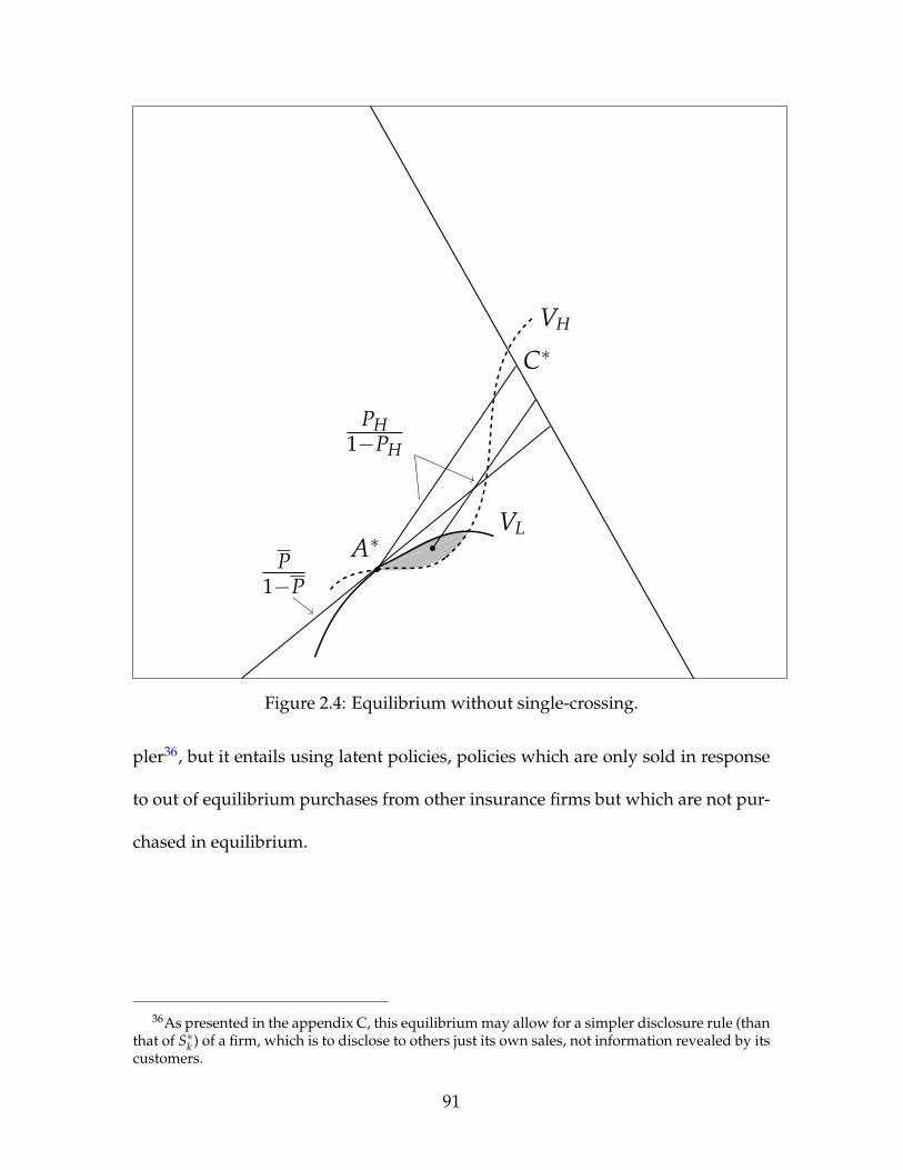
PH1−PH

P1−P

A∗

C∗VH

VL

Figure 2.4: Equilibrium without single-crossing.

pler36, but it entails using latent policies, policies which are only sold in response

to out of equilibrium purchases from other insurance firms but which are not pur-

chased in equilibrium.

36As presented in the appendix C, this equilibrium may allow for a simpler disclosure rule (thanthat of S∗k ) of a firm, which is to disclose to others just its own sales, not information revealed by itscustomers.

91

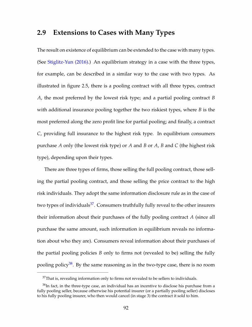
2.9 Extensions to Cases with Many Types

The result on existence of equilibrium can be extended to the case with many types.

(See Stiglitz-Yun (2016).) An equilibrium strategy in a case with the three types,

for example, can be described in a similar way to the case with two types. As

illustrated in figure 2.5, there is a pooling contract with all three types, contract

A, the most preferred by the lowest risk type; and a partial pooling contract B

with additional insurance pooling together the two riskiest types, where B is the

most preferred along the zero profit line for partial pooling; and finally, a contract

C, providing full insurance to the highest risk type. In equilibrium consumers

purchase A only (the lowest risk type) or A and B or A, B and C (the highest risk

type), depending upon their types.

There are three types of firms, those selling the full pooling contract, those sell-

ing the partial pooling contract, and those selling the price contract to the high

risk individuals. They adopt the same information disclosure rule as in the case of

two types of individuals37. Consumers truthfully fully reveal to the other insurers

their information about their purchases of the fully pooling contract A (since all

purchase the same amount, such information in equilibrium reveals no informa-

tion about who they are). Consumers reveal information about their purchases of

the partial pooling policies B only to firms not (revealed to be) selling the fully

pooling policy38. By the same reasoning as in the two-type case, there is no room

37That is, revealing information only to firms not revealed to be sellers to individuals.38In fact, in the three-type case, an individual has an incentive to disclose his purchase from a

fully pooling seller, because otherwise his potential insurer (or a partially pooling seller) disclosesto his fully pooling insurer, who then would cancel (in stage 3) the contract it sold to him.

92

α

β

VM

B

AD

C

VL

VH

P1−P

P−L1−P−L

PL1−PL

Figure 2.5: Equilibrium (A, B, C) with three types, which cannot be broken by Das individuals of higher-risk type supplement it by additional pooling insurance(along the arrow) without being disclosed to the deviant firm. P−L denotes theaverage probability of accident for the two highest risk types, while Vi indicatesan indifference curve for i-risk type (i = H, M, L).

93

for a cream-skimming deviant contract offering D that profitably attracts only low

or medium types, as riskier types are also induced to choose D39. This argument

can also be applied to the case with a continuum of types as well.

2.10 Previous Literature

In the more than four decades since RS appeared, its disquieting results have given

rise to a large literature, which we can divide into a few major strands. The first

looked for alternative equilibrium concepts, or game forms, under which equi-

librium might always exist, or under which a pooling equilibrium might exist.

Hellwig (1987) was the first to provide a game-theoretic framework in a dynamic

setting to analyze these equilibria (including RS) and contrast one with another.

Rothschild and Stiglitz (1997) reviewed the literature as it existed to that point,

suggesting that there had not yet been an adequate alternative resolution as to

what a competitive market equilibrium should look like in the presence of infor-

mation asymmetries. For instance, in Wilson (1977)’s reactive equilibrium , the

entry of even a very small firm induces all firms to "react," by withdrawing their

pooling contracts, making the deviant contract unprofitable and enabling the pool-

ing equilibrium to be sustained.4041

39By the same token, there is no incentive for contract manipulation40More recently Netzer and Scheuer (2014) have revived the Wilson-Miyazaki reactive equilib-

rium. Firms may "opt out" of the market after observing the contract offers of other firms. Theyshow that as long as the costs of opting out are nonzero, but not too large, there is a unique outcome- the Miyazaki-Wilson one.

41Mixed strategy equilibria (e.g. studied by Dasgupta and Maskin (1986) and Farinha Luz(2017), while interesting as an analytic solution, are unpersuasive as a description of what anymarket might look like. The notion that one might go to an insurance firm and choose among

94

A second strand more related to the analysis here has explored the conse-

quences of different information structures, in particular, the possibility of non-

disclosed contracts42. Most notable are a series of papers by Attar, Mariotti and

Salanie (2011, 2014, 2016). In the first (which is more akin to Akerlof’s model

of lemons and has a different scope of applications), they succeed in establishing

a condition for existence-the presence of an aggregate capacity constraint, along

with latent contracts. Their later 2014 model (which employs preferences that are

a generalization of the form considered in this paper) emphasizes the importance

of firms being able to offer a menu of contracts, but they get existence only under

very restrictive conditions-conditions which are never satisfied in our canonical

model. In their 2016 model, they allow firms to sell only a single contract, but,

again, in general, existence fails. More broadly, we consider a situation that is

closely related to those they study - all entail looking for equilibrium in a simple

adverse selection model - but ours is still markedly different from theirs; ours is the

natural one relevant in insurance markets, while they employ special assumptions

which make their analysis inapplicable to this market.

Their work highlights the important consequences of different information struc-

tures. The central objective of this paper, by contrast, is endogenizing the informa-

lotteries, which would assign probability distributions to benefits or premia, seems largely fanci-ful. Why that is so may necessitate an enquiry into behavioral economics, or into the economics oftrust: how does one know that, say, the contract has been drawn from the purported probabilitydistribution of contracts? One typically only sees one’s own outcome.

42See also the earlier papers of Jaynes (1978) and Ales and Maziero (2012). The latter focusedon the case of adverse selection in a non-exclusive environment, characterizing the conditions foran equilibrium to exist and showing that an equilibrium, if it exists, is a separating one where onlythe highest-risk type purchase full insurance at the actuarially fair price.

95

tion structure - allowing firms and individuals to decide what information to dis-

close to whom. The closest works to our paper within the adverse selection litera-

ture are Jaynes (1978), Jaynes (2011) and Hellwig (1988), who analyze a model with

a certain type of strategic communication among firms about customers’ contract

information. Jaynes (1978) characterizes an equilibrium outcome that involves

a pooling allocation plus supplemental provision at the high-risk price, the allo-

cation which our analysis (as well as that of Attar, Mariotti and Salanie (2016))

showed to be the only possible allocation. However, as clarified, in Jaynes (1978)’s

2-stage framework, the strategy of firms including the associated strategic commu-

nication is not a Nash equilibrium but a reactive equilibrium, with firms respond-

ing to the presence of particular deviant contracts, and thus Jaynes’ formulation

was subject to the same objections raised earlier. While our work differs from that

of Jaynes and Hellwig in several ways43, perhaps most important is that we con-

sider information revelation strategies by consumers as well as firms. This turns

out to be critical in the analysis of the existence of a Nash equilibrium, for it im-

portantly allows the creation of asymmetries of information about insurance pur-

chases between "established" firms and deviant firms. Without that, the pooling

contract would not be able to be sustained. As we have noted, there is a delicate

43Importantly, Hellwig’s analysis is based on a four-stage game, in which firms decide to whomthey send customer information (in stage 3) only after observing contract offers announced by firms(stage 1) and purchased by consumers (stage 2). In other words, their communication strategies areallowed to be conditional upon contract offers made by other firms. While Hellwig (1988) showsthat the Jaynes allocation (the equilibrium allocation in our paper) can be sustained as a sequentialequilibrium in the four-stage game, Jaynes (2011) attempted to characterize the "Jaynes allocation"as a perfect Bayes equilibrium in a two-stage game, in which firms announce their contract offersand communication strategies simultaneously. His formulation is thus markedly different fromthat presented here.

96

balance: on the one hand, one has to prevent overinsurance by high risk individu-

als purchasing pooling contracts (which requires established firms to know certain

information), and on the other hand, one has to prevent a deviant firm from having

enough information to enforce an exclusive contract that would break the pooling

equilibrium. The consumer and firm information strategies which we describe do

this, and it should be apparent that, at least in a simple game form, models relying

on just firm information strategies cannot do this, because they do not have the

information basis on which to engage in this kind of disclosure discrimination44.

2.11 The No-disclosure Limited Information Price

Equilibria

A final strand of literature to which this paper is related is that which assumes

no disclosure of insurance purchases, implying that the only information which a

firm has about the purchases of an individual are the sales the firm of the itself,

assuming that there is not anonymity in sales. This literature, however, does not

endogenize the decision not to disclose, but takes that policy as given. The stan-

dard assumption in the adverse selection literature (see e.g. Arrow (1965) is that

44That is, at least in the initial round of disclosures, firm disclosure can only be based on indi-vidual purchases. Assume some firms sold policies which did not disclose their sales. High riskindividuals would purchase such insurance beyond α, and the restriction that they not do so wouldnot be enforceable. Thus, the putative allocation could not be sustained, since the non-disclosurepooling contracts would make a loss. On the other hand, if firms sold only disclosure policies, thena deviant firm offering an exclusive contract in the region z would be able to enforce exclusivity,and this would break the pooling allocation. Hence, again, the putative equilibrium could not besustained. There has to be some basis on which firms can differentiate among whom to disclose;our consumer revelation mechanism provides this.

97

insurance firms and individuals simply take the price of insurance as given, and

consumers buy as much at that price as they want. Competitive equilibrium re-

quires that there be no profits (on average). Relating this to the literature, while RS

had full exclusivity and Akerlof had not exclusivity at all, this model posits that a

firm can monitor at least the purchases that it makes to the same individual, and

thus is able to track those.

More formally, we denote the purchase by a high risk individual at a price q(P)

corresponding to an accident probability P as αH(q(P)), and similarly for the low

risk as αL(q(P)) where q(P) = P1−P . The weighted average accident probability

when the price is q is then

P(q(P)) , PHθαH(q(P))αe(q(P))

+ PL(1− θ)αL(q(P))αe(q(P))

(2.6)

where αe(q(P)) = θαH(q(P)) + (1− θ)αL(q(P)), and

αL(q(P)) = arg max VL(α, β) s.t. β =P

1− Pα

and

αH(q(P)) = arg max VH(α, β) s.t. β =P

1− Pα

Since at any price, the high risk buy more insurance (αH(q) > αL(q)), the weighted

accident probability P(q(P)) is higher than the population weighted average P :

P(q(P)) > P. Now we define a (competitive) price equilibrium as Pe satisfying the

following conditions: (a) (uninformed) sellers have rational expectations Pe about

98

the weighted average accident probability of the buyers; (b) with those rational ex-

pectations, prices are set to generate zero profits; and (c) at those prices consumers

buy the quantities that they wish45. Thus, a price equilibrium Pe satisfies

Pe = P(q(Pe)) with P ′q ′ > 0 (2.7)

Low risk individuals diminish their purchases of insurance as prices increase. This

is the well-known adverse selection effect. But the value of P ′(q ′) depends on the

elasticities of demand of the two groups as well as their relative proportions, and

so in general there may be more than one price equilibrium. A sufficient condition

for a unique equilibrium, in which only high risk individuals purchase insurance,

is αL(q(PH)) = 04647. Nash equilibrium and non-existence of a partial information-

no disclosure price equilibrium. In the no-disclosure price equilibrium, the insur-

ance firms simply take the price as given. However, while a firm doesn’t know the

size of the policies taken up by an individual from other firms, he knows what he

has sold48. An insurance firm can offer a large policy - he knows to whom he sells,

and can refuse to sell a second policy to the same individual49. We define a partial

45The latter conditions are equivalent to the standard conditions of demand equaling supply forthis particular model.

46αL(q(PH)) = 0 implies PL1−PL

U ′(W−d)U ′(W)

≤ PH1−PH

47We could define a price equilibrium in a Nash-Bertrand fashion by adding another conditionthat each firm, taking the prices of others as given, chooses the price which maximizes its profits.In this case, it can be shown that there exists a unique price equilibrium, the lowest price at whichequation 2.7 is satisfied.

48This would not be the case if individuals purchased insurance about an event affecting a thirdparty, and firms sold such insurance without knowledge of the purchaser.

49In the context of moral hazard, the implication of this simple observation were explored inArnott and Stiglitz (1991a) and Arnott and Stiglitz (1987).

99

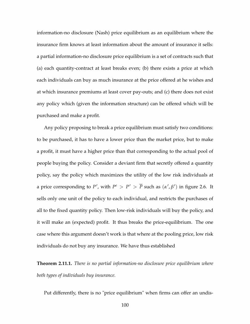
information-no disclosure (Nash) price equilibrium as an equilibrium where the

insurance firm knows at least information about the amount of insurance it sells:

a partial information-no disclosure price equilibrium is a set of contracts such that

(a) each quantity-contract at least breaks even; (b) there exists a price at which

each individuals can buy as much insurance at the price offered at he wishes and

at which insurance premiums at least cover pay-outs; and (c) there does not exist

any policy which (given the information structure) can be offered which will be

purchased and make a profit.

Any policy proposing to break a price equilibrium must satisfy two conditions:

to be purchased, it has to have a lower price than the market price, but to make

a profit, it must have a higher price than that corresponding to the actual pool of

people buying the policy. Consider a deviant firm that secretly offered a quantity

policy, say the policy which maximizes the utility of the low risk individuals at

a price corresponding to P ′, with Pe > P ′ > P such as (α ′, β ′) in figure 2.6. It

sells only one unit of the policy to each individual, and restricts the purchases of

all to the fixed quantity policy. Then low-risk individuals will buy the policy, and

it will make an (expected) profit. It thus breaks the price-equilibrium. The one

case where this argument doesn’t work is that where at the pooling price, low risk

individuals do not buy any insurance. We have thus established

Theorem 2.11.1. There is no partial information-no disclosure price equilibrium where

both types of individuals buy insurance.

Put differently, there is no "price equilibrium" when firms can offer an undis-

100

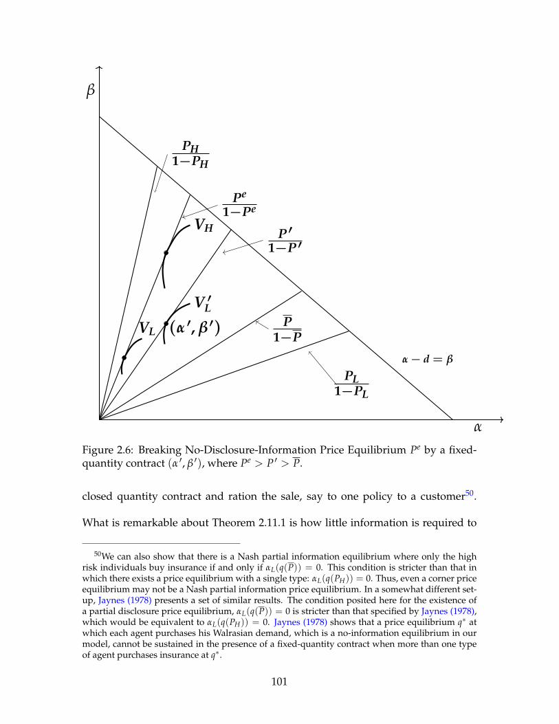
α

β

α− d = β

P1−P

(α ′, β ′)

V ′LVL

VH

PL1−PL

P ′1−P ′

Pe

1−Pe

PH1−PH

Figure 2.6: Breaking No-Disclosure-Information Price Equilibrium Pe by a fixed-quantity contract (α ′, β ′), where Pe > P ′ > P.

closed quantity contract and ration the sale, say to one policy to a customer50.

What is remarkable about Theorem 2.11.1 is how little information is required to

50We can also show that there is a Nash partial information equilibrium where only the highrisk individuals buy insurance if and only if αL(q(P)) = 0. This condition is stricter than that inwhich there exists a price equilibrium with a single type: αL(q(PH)) = 0. Thus, even a corner priceequilibrium may not be a Nash partial information price equilibrium. In a somewhat different set-up, Jaynes (1978) presents a set of similar results. The condition posited here for the existence ofa partial disclosure price equilibrium, αL(q(P)) = 0 is stricter than that specified by Jaynes (1978),which would be equivalent to αL(q(PH)) = 0. Jaynes (1978) shows that a price equilibrium q∗ atwhich each agent purchases his Walrasian demand, which is a no-information equilibrium in ourmodel, cannot be sustained in the presence of a fixed-quantity contract when more than one typeof agent purchases insurance at q∗.

101

break the price equilibrium: the firm just uses its own contract information to im-

plement the quantity constraint. It is natural to ask, if there is not a price equilib-

rium, is there some analogous equilibrium, with say just fixed quantity contracts?

Consider a case where the two groups are quite similar. Each insurance firm sells

insurance in fixed units, say (α, β), say the policy which is most preferred by the

low risk individual along the break-even pooling line. The high risk individual

would not want to buy two units of that insurance. But he would supplement

his purchase with the undisclosed insurance at his own price, in an amount that

brings him to full insurance. The analysis of this paper has shown that this kind

of pooling contract cannot be an equilibrium: there is always a deviant policy that

could be offered that would be taken up only by the low risk individuals, given

the posited information structure. In other words, given this partial information

structure, there is no equilibrium, ever, where both groups buy insurance. By con-

trast, with the more complex endogenous information structure described in the

paper, there is always an equilibrium.


In insurance markets with asymmetric information, firms will use what informa-

tion is available to make inferences about purchasers of insurance, including in-

formation about the amount of insurance purchased. High risk individuals know

this, and have an incentive to do what they can to ensure that insurance firms

can’t tell that they are high risk, and to try to keep any relevant information (such

102

as the amount of insurance purchased) secret, and there may be market incentives

for firms to comply. The earlier work of Akerlof and RS had, of course, shown

the importance of the information structure: information about insurance pur-

chased conveyed important information about the individual’s type, and there-

fore, whether that information was available was central in determining the nature

of the equilibrium. The differences between Akerlof and RS reflected differences

in assumptions about the information structure, e.g. RS assumed sufficient infor-

mation to enforce exclusivity. Allowing undisclosed contracts and incorporating

realistic assumptions about things that insurance firms know, in particular, that

they know the identities of their customers and the quantities purchased, destroys

both the RS and the Akerlof equilibria. Expanding the equilibrium construct to

include endogenous information disclosure rules is complex, but in fact helps re-

solve some longstanding conundrums in information economics, in particular the

general non-existence of pooling equilibria and the possible non-existence even of

a screening equilibrium. When we endogenize information revelation, the unique

equilibrium allocation is a partially disclosed pooling contract - the pooling con-

tract most preferred by the low risk individual51 - plus undisclosed supplemental

insurance for the high risk individuals and no supplemental insurance for the low

risk individuals. The equilibrium endogenously creates asymmetries in informa-

tion about insurance purchases; we show that at least within our framework, such

asymmetries are essential to supporting the equilibrium. In some ways, the equi-

51That is, the pooling allocation at the population weighted accident probabilities most preferredby low-risk individuals. (This pooling contract is that upon which Wilson (1977) focused.)

103

librium that arises with endogenous information looks much more like observed

equilibria: Equilibrium always exists, and always entails some pooling. Moreover,

the analysis and its results do not rely on the highly restrictive single crossing prop-

erty which has been central in the literature spawned by RS. The insurance model

has proven a useful tool for analyzing more generally markets with asymmetric

information, and the papers analyzing imperfect and asymmetric information in

that context have spawned a huge literature, with the concepts being applied to

a rich variety of institutional structures52. The natural information assumptions

concerning potentially hidden actions and hidden characteristics differ across mar-

kets. This paper has raised questions about both the Akerlof and RS analyses, and

by implication, the results in the large literature based on them.

We hope that this paper will, like the earlier RS and Akerlof analyses, spawn

further research in the context of other markets in the analysis of market equi-

librium with asymmetric information where contracts and the information struc-

ture/revelation are endogenously and simultaneously determined.

2.13 Appendices

Appendix A: Proof of Lemma 2.6.2.

Given lemma 2.6.1, the consumer purchasing more than α must not reveal his full

52It is important to recognize that, for the most part, these models of insurance were not in-tended to provide a good institutional analysis of the insurance market; rather, the insurancemarket provided the paradigm for studying behavior in, for example, labor, product, and cap-ital markets because it seemed so simple to strip away institutional details, and study marketsunencumbered by them. It was for this reason that these paradigmatic models proved so fruitful.The analysis of this paper should be taken in the same spirit.

104

purchases to any firm. Assume there are N purchases and that the firm j to which

he is most dishonest has been given information about N-1 purchases, and in par-

ticular, he does not reveal purchases from k. Then j reveals to k information about

all purchases but that of k; but then k knows about all purchases, and that the indi-

vidual’s total purchases exceed α. Assume now that the firm j to which he is most

dishonest has been given information about N-2 purchases, i.e. the consumer does

not reveal purchases from k and k ′ . Either k knows about k ′ or not. If k knows

about k ′, then when j reveals all of its information to k, then k knows about all

purchases. If k does not know about k ′ , then when k and j reveal all of their infor-

mation to k ′, k ′ knows about all purchases. The argument can be extended to any

level of non-disclosure.

Appendix B: Proof of Theorem 2.6.3.

It is obvious that by Lemma 2.6.2, the strategy S∗k generates the equilibrium alloca-

tion E∗. We will now show the strategy S∗k sustains E∗ against any deviant contract.

Note first that a deviant firm cannot make profits by attracting only high-risk indi-

viduals in the presence of non-established firms offering any amount of insurances

at qH. This is because then no individual would pay a price higher than qH since a

deviant firm, even with CM, cannot induce the established firms (with S∗k ) to offer

more than α at q under any circumstance. If the deviant attracts both high and low

risk, his contract would have to lie on or below the pooling line, and the best that

he could be expected to do is zero profits. A deviant firm can thus make positive

105

profits only by attracting only low-risk types.

Lemma 2.13.1. A necessary condition for a deviant contract to attract only low risk in-

dividuals is that the contract be in the non-empty region z in figure 2.2, the set of (α, β)’s

such that

VL(α, β) > V∗L and β− qα ≥ qH(α− α), (2.8)

where V∗L is the expected utility of the low risk individuals in the putative equilibrium.

Clearly, when the first inequality is not satisfied, the low risk individuals will

not purchase the policy, and when the second condition is not satisfied, the high

risk individual will purchase the policy, supplementing it with the secret insur-

ance. Consider any policy D(= (αD, βD)) in z (satisfying the above two condi-

tions). Given the equilibrium strategies of the established firms, then high risk

individuals will buy D, supplementing it with pooling insurance from the estab-

lished firms, bringing the entire purchases (of revealed insurance) at least to α.

Given the conditions imposed on preferences (quasi-concavity, slope of indiffer-

ence curve equaling qH with full insurance)53, high risk individuals will wish to

buy as much insurance at the pooling odds as they can. With full disclosure, they

can buy α. Since individuals have a choice of disclosure, they can at least get α with

full disclosure to established firms but with no disclosure to the firm offering D.

Denote by D ′ total insurance (D plus the pooling contract plus the supplemental

secret insurance). It is obvious that VH(D ′) > VH(A∗). With the given consumer

and firm disclosure strategies, no firm will disclose to the deviant firm their sales to

53As discussed in section 2.7, our results hold even with preferences that are not quasi-concave.

106

the insurance, so that the deviant firm cannot enforce the restrictions necessary to

prevent consumers from buying supplemental pooling insurance. It follows that

there exists no policy breaking the pooling contract A∗54.

Appendix C: An Alternative Equilibrium

In this appendix, we show that the equilibrium allocation can be supported by

alternative contracts, entailing different restrictions and disclosures. We now as-

sume that restrictions are based not just upon the amount of insurance purchased

but also upon the price (equivalently, on both α and β), and when consumers and

firms disclose information, they disclose not just the amount of insurance, but the

price at which they purchased insurance. Assume the established firms55 have a

strategy S0k which entails the same disclosure rule about to whom to disclose as

54Two minor subtleties: While we showed that in equilibrium, there is no contract manipulation,we have to show that no deviant firm will engage in CM. But it is obvious (by our earlier analysis)that CM is attractive only to high risk individuals. This implies that no deviant strategy with CMcan attract low-risk types only by charging q ∈

(PL

1−PL, P

1−P

), since no deviant strategy without CM

can. Secondly, our earlier analysis established that the deviant firm would not be able to enforcethe exclusivity it needed regardless of the information disclosure strategy of the deviant firm.

55We also assume, as before, that the other firms (j=M+1, –, N) offer any amount of insurance ata price qH without disclosure. There is a single deviant firm.

107

that of S∗k56 while offering

α =

α at a price q if the individual has no other insurance

0 if the individual has purchased other insurance at a price higher than or equal to q

αk ≤ α(D) at the price q if the individual has purchased elsewhere a contract D

that offers insurance αD at a price q < q,(2.9)

where α(D) is the maximum amount of insurance that a low risk individual would

want to purchase to supplement the contract D at the pooling odds. Because the

low risk individual is better off than at A∗, α(D) + αD > α, while α(D) ≤ α with

the inequality holding for αD > 057. In words, the established firms with Sok sell

the full contract A∗ (and only that contract) to an individual with no other insur-

ance (so far as it knows); sells nothing to anyone who has purchased any other

insurance at less (or at equally) attractive terms than the pooling equilibrium (it

can infer that such a person is a high risk individual); and sells a variable amount

of insurance, bringing total insurance purchased up to, at a maximum an amount

α(D) at the pooling price if the individual has purchased a contract D at a lower

price than q.

The equilibrium looks precisely as before, except now everyone purchases the

policy A∗ from a single insurance firm. Out of equilibrium behavior entails the

56The disclosure rule of S0k can be simpler than that of S∗k ; firms need disclose to others their own

sales only, not information revealed by their customers, because every consumer purchases α at aprice α in equilibrium.

57α(D) = arg maxαPLU(W − d + α + αD) + (1− PL)U(W − qα− qαD) with PL1−PL

≤ q ≤ q

108

use of latent contracts, the policies the sale of which are only triggered when indi-

viduals have purchased a deviant contract, D. It should be clear that no low risk

individual will buy any policy sold at a price above q. Accordingly, any policy

sold at a price between qH and q loses money. Also, since the amount of additional

pooling insurance offered on top of any insurance revealed to be purchased else-

where is not greater than α, no high-risk individuals would be willing to pay an

average price higher than qH (getting some part of the package at a price below

q.) to trigger the sale of αk58. Thus we can focus on deviant policies sold at a price

below q. High risk individuals will supplement D, topping up total purchases to

α(D) of insurance. But that means that expected utility of the high risk individual,

supplementing D with the pooling contract (up to α(D)), and supplementing that

with secret insurance (at its own odds) is higher than at the original allocation, i.e.

the high risk individual as well as the low risk individual buys D, and that means

that D loses money, since D is sold at a price below q (i.e. is below the pooling

line.) It is thus clear that this simple strategy can support the equilibrium5960.

58Thus, if the individual chose not to reveal any purchase from the deviant firm, he could havepurchased at q an amount α. Earlier, we referred to the kind of deception where an individualpurchases two policies (perhaps bundled, as here) and discloses only one as contract manipulation.

59As before, it is important that the deviant firm not be able to enforce exclusivity, and theinformation strategy ensures that this is the case.

60In the main text, we showed that the pooling contract cannot be broken except possibly by acontract in the area z, and a straightforward adaptation of the arguments there apply here. Theanalysis here implies that even contracts in z cannot break the putative equilibrium.

109

Appendix D: Deviants Offering Multiple Contracts at Different

Prices

In this appendix, we show that our results hold even when firms are allowed to

sell multiple contracts at different prices. The central issue is whether this allows

a deviant firm to break our putative equilibrium by taking advantage of cross-

subsidization. A deviant firm does so to induce self-selection among the appli-

cants - with the self-selection process reducing the costs of the high risk individuals

buying insurance from the deviant. We first explain why the set of strategies con-

sidered earlier now doesn’t "work". We then describe intuitively the challenges

involved in finding an equilibrium strategy. Next we provide the formal analy-

sis, establishing the main theorem of this appendix. Let (A∗, C∗) represent the

equilibrium allocation described earlier. Now consider the deviant pair of policies

(A∗B, G) (as depicted in figure 2.7), where A∗B entails an offer of αS at q without

disclosure and G offers αD at a price q lower than q with disclosure and with G

being offered conditional on no additional insurance being purchased. There al-

ways exists a continuum of pairs of policies (A∗B, G) such that G is chosen by all

the low-risk individuals while A∗B is chosen by all the high-risk who simultane-

ously buy A∗, that is, the high risk individuals supplement A∗B with the pooling

insurance A∗, i.e. they buy α of insurance from the established firms and αS from

the deviant firm. Because the price q is greater than pL1−pL

, the deviant firm makes

a profit on G even though it makes a loss on the contract purchased by the high

risk individuals. By carefully choosing (A∗B, G) or αS, (αD, q), the deviant firm

110

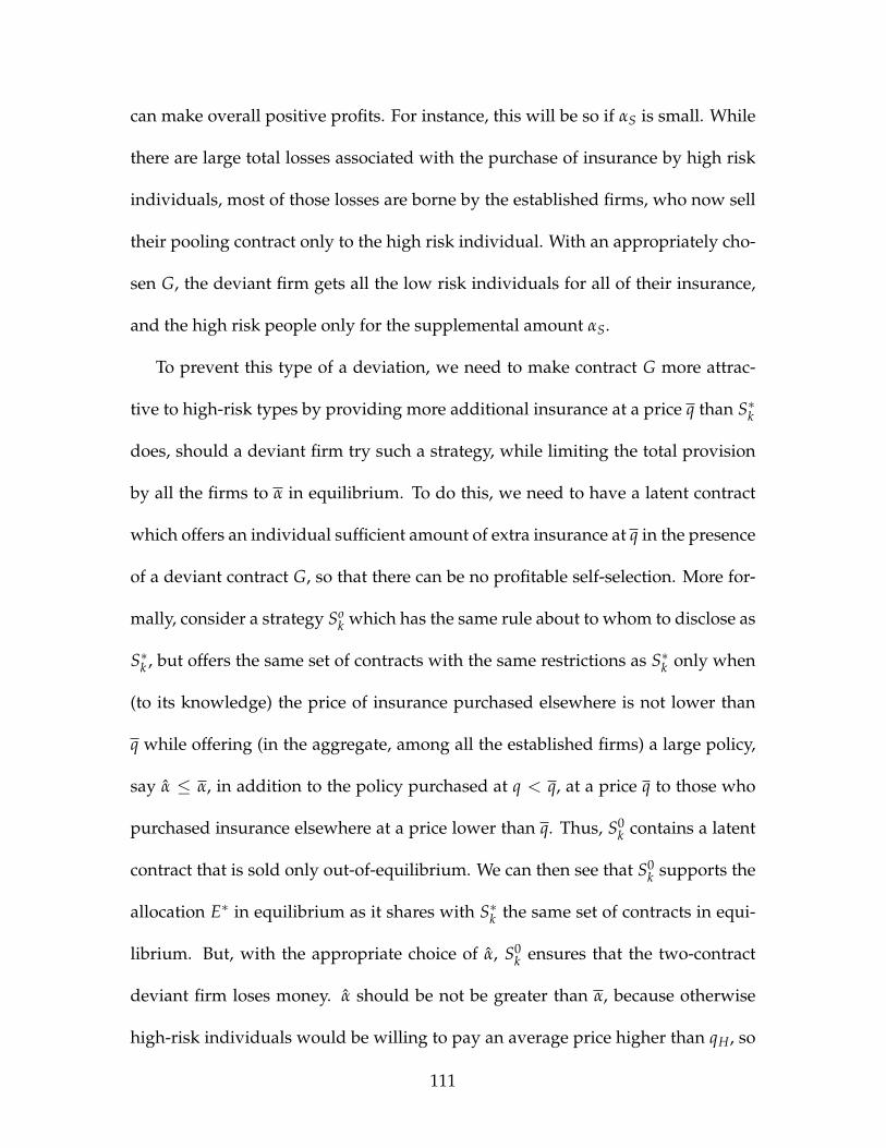
can make overall positive profits. For instance, this will be so if αS is small. While

there are large total losses associated with the purchase of insurance by high risk

individuals, most of those losses are borne by the established firms, who now sell

their pooling contract only to the high risk individual. With an appropriately cho-

sen G, the deviant firm gets all the low risk individuals for all of their insurance,

and the high risk people only for the supplemental amount αS.

To prevent this type of a deviation, we need to make contract G more attrac-

tive to high-risk types by providing more additional insurance at a price q than S∗k

does, should a deviant firm try such a strategy, while limiting the total provision

by all the firms to α in equilibrium. To do this, we need to have a latent contract

which offers an individual sufficient amount of extra insurance at q in the presence

of a deviant contract G, so that there can be no profitable self-selection. More for-

mally, consider a strategy Sok which has the same rule about to whom to disclose as

S∗k , but offers the same set of contracts with the same restrictions as S∗k only when

(to its knowledge) the price of insurance purchased elsewhere is not lower than

q while offering (in the aggregate, among all the established firms) a large policy,

say α ≤ α, in addition to the policy purchased at q < q, at a price q to those who

purchased insurance elsewhere at a price lower than q. Thus, S0k contains a latent

contract that is sold only out-of-equilibrium. We can then see that S0k supports the

allocation E∗ in equilibrium as it shares with S∗k the same set of contracts in equi-

librium. But, with the appropriate choice of α, S0k ensures that the two-contract

deviant firm loses money. α should be not be greater than α, because otherwise

high-risk individuals would be willing to pay an average price higher than qH, so

111

α

β

α− d = β

VL

α

β

G

αDα + αS

α + αD

α + αS ′

A∗B P1−P

PL1−PL

PH1−PH

A∗B ′

A∗

Figure 2.7: Nash Equilibrium can be sustained against multiple deviant con-tracts (A∗B, G) or (A∗B ′, G) offered at different prices as high-risk individuals alsochoose G (over A∗B) or as (A∗B ′, G) yields losses for the deviant firm (while in-ducing self-selection).

112

that through contract manipulation they could purchase α. We set α = α. Now we

will focus upon a cream-skimming strategy G, which offers αD at price q below q.

A high-risk individual i choosing G would not reveal to the deviant firm d his pur-

chases of pooling insurance from other firms, but has an incentive to reveal to the

established firms his purchase of low price insurance, for that triggers the offer of

supplemental insurance. But given the strategy S0k , that means that the established

firms don’t disclose their sales to the deviant, which ensures that the exclusivity

provision associated with G cannot be enforced. Knowing this, to induce self-

selection, a deviant firm offers a "large" contract (A∗B ′) - entailing insurance of

α ′S without disclosure. Given a choice between G and (A∗B ′), all high risk indi-

viduals choose (A∗B ′) and all low risk individuals choose G. We can then show

that any pair of contracts (G, A∗B ′) that induces self-selection makes losses. To see

this, note that if a high risk individual purchases A∗B ′ without disclosure, his total

insurance purchased at q is αS + α. The high risk individual then supplements this

with secret insurance at price qH bringing him to full insurance. By contrast, with

policy G (disclosed) the individual gets (αD + α) at a total premium of (qαD + qα).

The high risk individual then supplements this with insurance at price qH bring-

ing the individual to full insurance. It is easy to show that self- selection requires

qH(αS ′ + α)− (αD + α) ≥ q(αS ′ + α)− (qαD + qα) (2.10)

113

Condition (8) can be rewritten as

αD ≤ (qH − q)−1(qH − q)αS ′

The corresponding profit πG, A∗B ′ for the deviant firm is

πG, A∗B ′ = −θα ′S(qH − q) + (1− θ)αD(q− qL)

≤ αS ′(qH − q)(qH − q)−1[−θ(qH − q) + (1− θ)(q− qL)]

= α ′S(qH − q)(qH − q)−1[q− q] < 0

i.e., the total profit for the deviant firm is negative. Alternatively, if the deviant

firm fails to "separate," so the high risk individuals chooses G, the deviant firm

loses money. We have thus established

Theorem 2.13.2. If deviant firms are allowed to offer multiple insurance contracts, there

always exists an equilibrium strategy that sustains the unique equilibrium allocation E∗ .

The Nash equilibrium entails the use of latent contracts, while it does not re-

quire preferences to satisfy the single-crossing property.

114

Chapter 3

Mediated Persuasion: First Steps

3.1 Introduction

How does the presence of a mediator affect the informational interaction between

two parties? In this paper we study a game of persuasion between one side (a

sender) that is trying to persuade another side (a receiver) to take a certain action;

we add to this standard environment a mediator who is able to alter the recom-

mendation of the sender in some way, before the receiver takes his action.

The subject of persuasion, broadly construed, is currently being actively inves-

tigated in information economics; much excellent research has been produced in

the last few years on this, and the topic is continuing to prove a fertile ground

for models and applications. More particularly, the topic of information design

- the study of how information endogenously affects incentives and vice versa -

is swiftly becoming a major avenue of research. We add an institutional aspect

to this research program, and investigate the effects of different informational-

organizational topologies on information revelation and welfare.

In the model studied here, the sender and the receiver are restricted to commu-

nicate indirectly, via an intermediator (perhaps more than one), due to technical on

115

institutional constraints. For example, when a financial firm issues certain kinds

of financial products, some large (institutional) investors are prohibited from pur-

chasing them, unless they have been rated by a third party, and have achieved a

certain rating. Similarly, in many organizations (including many firms, the mil-

itary, and the intelligence community) the flow of information is directed, with

various people having the ability to alter (or perhaps not pass on) the information

passed up to them. This is precisely the kind of setting we are concerned with

here.

Our work relies on some results, and is in the spirit of, the celebrated "Bayesian

persuasion" approach of Kamenica and Gentzkow (2011) (referred to simply as

"KG" for brevity hereafter) who consider a simpler version of this problem, and

discuss an application of a certain concavification result first considered in chapter

1 of Aumann and Maschler (1995). Sah and Stiglitz (1986) introduced the analy-

sis of economic systems organized in parallel and in series1; hierarchies and pol-

yarchies of persuasion via provision of information have already been explored in

previous work (Gentzkow and Kamenica (2017a) (referred to as "GK" henceforth,

not to be confused with "KG"),

There are three papers that are closely related to the present model. One is

Ambrus, Azeveda and Kamada (2013) which considers a cheap talk model where

the sender and receiver also communicate via chains of intermediators. Our work

is similar in that talk is "cheap" here as well, meaning that the specific choices

of the sender and the mediators do not enter their utility functions directly and

1The terminology is derived from analogous ways of connecting electric circuits.

116

only do so through the action of the receiver; in addition, we, too, have an anal-

ogous communication sequence. The difference is that the sender is not perfectly

informed about the state, and the message he sends depends on the state, and

is in general, stochastic. Li and Norman (2017)’s paper on sequential persuasion

serves as another stepping stone - they have a very similar model of persuasion,

except that the senders move sequentially, observing the history of actions of the

senders who moved before them (unlike in our model). The other relevant work

is Gentzkow and Kamenica (2017)’s work on competition in persuasion where the

senders move simultaneously (like in our model), but all senders are trying to pro-

vide information about the state of the world,. whereas we study an environment

where the mediator is trying to provide information about the realization of the

sender’s experiment.

Perez-Richet and Skreta (2017) present a complementary model that differs in

one key respect - the mediator (using our nomenclature) moves first and his choice

is observed by the sender before the sender acts. Our focus is on analyzing out-

comes of a particular game as one changes preferences for the mediator, fixing the

state spaces, while they focus on equilibria of a game where the preferences of the

mediator are always fully aligned with those of the receiver.

Strulovici (2017) in his "Mediated Truth" paper explores a somewhat related

environment where a "mediator" - an expert of some sort or a law enforcement of-

ficer - has access to information that is "costly to acquire, cheap to manipulate and

produces sequentially". He shows that when information is reproducible and not

asymptotically scarce (for example, one can perform many scientific experiments)

117

then societies will learn the truth, while when information is limited (such as ev-

idence from a crime) the answer is negative. In our work we consider a one-shot

game, but his insight provides an interesting contrast. For example, a repeated ver-

sion of the game considered here would satisfy the condition for evidence to not

be asymptotically scare, however, it is not clear that this is enough to overcome the

incentive problem when the mediator can only garble the signals; certainly there

will be no learning is the unique equilibrium in our model is uninformative, as can

be the case.

Ichihashi (2017) studies a model in which the sender’s information may be lim-

ited; he focuses on the cases where doing so might benefit the receiver. In our

model a similar role is played by the mediator who modifies the information pro-

duced by the sender, and can only modify it by garbling (i.e. only decreasing the

amount of information). Thus, while Ichihashi (2017) limits the sender’s informa-

tion, we limit what the sender can do with that information.

We study a game where the players move simultaneously (this is just a model-

ing trick of course - they do not have to actually act at the same time - the reason

for this is because typically one party is not aware of the ratings mechanism or

the choice of the financial instruments of the other party when committing to an

action; it could also be simply because a player is unable to detect deviations in

time to adjust their own strategy); they key point is that the mediator does not see

the choice of the sender before making his own choice as in some other models.

In other words, we assume "double commitment" - commitment to an information

structure for the sender and the mediator, along the lines discussed in KG. This

118

feature generates an interesting possibility of having a kind of prisoner’s dilemma

not in actions, but in information2. The flow of information is path-dependent

(as in Li and Norman (2017)), yet not quite sequential while action choices for the

sender and the mediator are simultaneous.

Our focus will be on the amount of information revealed in various organi-

zational setups and the effect of competition and preference (mis)alignment on

information revelation and outcomes. Although the basic model is quite general,

we have in mind one particular application - the design of a ratings agency. A

rating assigned to a financial product can be thought of as an expression of likeli-

hood of default or expected economic loss. A firm (in the parlance of the present

setting, the sender) chooses strategically what evidence to submit to a rater (here,

the mediator). The mediator, perhaps driven by concerns that may not be identical

to those of the firm, then rates the evidence submitted by the firm, and issues a

recommendation to the client or the public. We analyze the effect on informative-

ness and welfare of the mediator’s presence in this informational-organizational

topology.

There are several features of this real-world example that deserve mention.

First note that the issuing firm itself cannot rate its own financial products; it does,

however, design its products (or at least gets to choose the products that it submits

for review at a particular instance). The ratings agency cannot choose the products

- it is constrained to rate the package it has been submitted, but it can choose its

ratings process and criteria. It also exhibits the criteria according to which it is-

2This is also discussed in GK.

119

sued its conclusions. Finally, the purchaser of the financial products (the receiver)

is often required to only buy products that have been rated by a reputable firm - in

other words, there is an institutional constraint at work.

To take a specific example consider structured finance products that consisted

of various repackagings of individual loans (mortgages were by far the most im-

portant component) into so-called structured investment vehicles, or SIVs. The

financial firms issued products that consisted of bundles of individual mortgages,

along with rules for obtaining streams of payments from those mortgages. These

streams were correlated with each other (since two nearby houses were in the same

area, the local economic conditions that affected the ability of one lender to repay,

also affected the ability of the other lender to repay), as well as with the overall

economy. The firms chose the specific mortgages that went into each SIV strategi-

cally. The ratings agencies then rated these SIVs; however, one key element in their

ratings (and one that was later shown to be partially responsible for the revealed

inaccuracy of those ratings) is that the ratings agencies did not provide their rat-

ings based on the correlations of the returns with the overall economy. Rather,

their ratings consisted (mostly) of evaluations of correlations of individual finan-

cial products in an SIV with each other. The issuer clearly wants to achieve as high

a rating as possible3, but if the preferences of the mediator are to "collude" with the

seller, this essentially means that there may be very little information revelation in

equilibrium.

3And in fact, there is evidence in structured finance that the firms did design their products sothat the senior tranches would be as large as possible, while still getting the highest possible rating.

120

In this example the state of the world is a complete, fully specified joint distri-

bution of returns; an experiment is a mapping from states of the world into a set

that specifies only partial information about the correlations (for example, indi-

vidual correlations)4. The mediator then designs a signal (a rating procedure) that

maps information about individual correlations into a scaled rating.

In single-issuer bonds, ratings are mute about correlations with other bonds or

with the market. In 2007, less than 1% of corporate issues but 60% of all structured

products were rated AAA. 27 of 30 AAA issues underwritten by Merril Lynch in

2007, were by 2008 rated as speculative ("junk") (See Coval, Jurek and Stafford

(2008)). We suggest that a possible explanation for this is that if the mediator is

unable to provide new information, and is only able to "garble" or rely on the in-

formation provided to it by the issuer, then the equilibria in general will not be

very informative (and in fact, as the preferences of the mediator and the sender

diverge, the only equilibrium that survives is uninformative). This reasoning sug-

gests a policy proposal - requiring the ratings agencies to perform independent

analysis (say, additional "stress tests") on the products they are rating, to increase

the informativeness of the rating.

In what follows we investigate the effect of adding a mediator to a persua-

sion environment as well as the welfare implications (for all parties) of varying the

alignment of preferences of the sender and the mediator. In addition, we consider

the effect of adding additional mediators. Finally, we give a novel characteriza-

tion of the set of feasible beliefs for this game and discuss its several interesting

4The "big three" firms all utilize fairly coarse scales for ratings.

121

features. We do not give a full characterization of equilibria as a function of prefer-

ences (this is a difficult fixed point problem); rather, we give suggestive examples

and provide intuition.

3.2 Environment

We study a game with n ≥ 3 players; The first player is called the sender and the

last player is called the receiver. The remaining players are the mediators; if there

are more than one of them, we also specify the order in which their probabilistic

strategies are executed.

We fix a finite state space, Ω (consisting of nΩ elements) and a finite realiza-

tion space5 E (consisting of nE elements), where to avoid unnecessary trivialities,

the cardinality of the set of signals is weakly greater than that of the set of states.

An experiment for the sender is a distribution over the set E, for each state of the

world: X : Ω → ∆(E); denote by X the set of available experiments. We assume

that X contains both the uninformative experiment (one where the probabilities

of all experiment realizations are independent of the state) and the fully reveal-

ing experiment (where each state is revealed with probability one). To distinguish

between the choices of the sender and those of the mediator, we define a signal

for the mediator to be a function M : E → ∆(S) where S is the space of signal

realizations containing nS elements; let M denote the set of available experiments.

Put differently, the mediator is choosing distributions of signal realizations condi-

5Typically, the realization space is part of the choice of the sender; here we fix this space (whilekeeping it "rich enough") to isolate the effects of mediated persuasion.

122

tional on realizations of experiments6. All available experiments and signals have

the same cost, which we normalize to zero. We also refer to either an experiment,

or a signal, or their product, generically as an information structure. Since the state

space and all realization spaces are finite, we represent information structures as

column-stochastic matrices with the (i, j)’th entry being the probability of realiza-

tion i conditional on j. Finally, the receiver takes an action from a finite set A (with

nA elements; we assume that nA ≥ nS = nE ≥ nΩ to avoid trivialities associated

with signal and action spaces not being "rich" enough). The utility of the sender is

denoted by uS(ω, a), that of the mediator by uM(ω, a) and that of the receiver by

uR(ω, a). We assume for concreteness that if the receiver is indifferent between two

or more actions given some belief, he takes the action that is best for the sender.

This setup is capturing one of the key features of our model - the space of re-

alizations of experiments for one player is the state space for the following player.

In other words, both the sender and the mediator are choosing standard Blackwell

experiments, but with different state and realization spaces.

For clarity, we summarize the notation used at this point: we use the conven-

tion that capital Greek letters (X, M) refer to the distributions, bold capital Greek

letters (X, M) refer to sets of distributions, small Greek letters (χ, µ) refer to (pure)

strategies of the players, capital English letters (E, S) refer to spaces of realizations

for information structures, and small English letters (e, s) refer to realizations.

The timing of the game is fairly simple: the sender and the mediator choose

6We later explore a different and richer environment where the mediator can choose realiza-tions of signals conditional on both experiment realizations and states of the world.

123

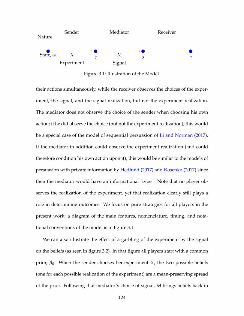
Nature

State, ω e s a

Sender Mediator Receiver

X

Experiment

M

Signal

Figure 3.1: Illustration of the Model.

their actions simultaneously, while the receiver observes the choices of the exper-

iment, the signal, and the signal realization, but not the experiment realization.

The mediator does not observe the choice of the sender when choosing his own

action; if he did observe the choice (but not the experiment realization), this would

be a special case of the model of sequential persuasion of Li and Norman (2017).

If the mediator in addition could observe the experiment realization (and could

therefore condition his own action upon it), this would be similar to the models of

persuasion with private information by Hedlund (2017) and Kosenko (2017) since

then the mediator would have an informational "type". Note that no player ob-

serves the realization of the experiment, yet that realization clearly still plays a

role in determining outcomes. We focus on pure strategies for all players in the

present work; a diagram of the main features, nomenclature, timing, and nota-

tional conventions of the model is in figure 3.1.

We can also illustrate the effect of a garbling of the experiment by the signal

on the beliefs (as seen in figure 3.2). In that figure all players start with a common

prior, β0. When the sender chooses her experiment X, the two possible beliefs

(one for each possible realization of the experiment) are a mean-preserving spread

of the prior. Following that mediator’s choice of signal, M brings beliefs back in

124

β0 10

β(X, eL) β(X, eH)0 1

0 1β(MX, sL) β(MX, sH)

Figure 3.2: Effect of Garbling on Beliefs in a Dichotomy.

in a mean-preserving contraction. In other words, in terms of figure 3.2, we can

say that the mediator chooses the length (but not the location) of the two arrows,

and the sender chooses the outer endpoint for each arrow. The inner point of each

arrow represents the final beliefs.

Denote by βA(ω|s) the posterior belief of the receiver that the state of the world

is ω, computed after observing information structure A, and a signal realization s

and denote by βA(s) the full distribution. We will also find it convenient to refer

to distributions of distributions, which we will denote by τ so that τA(β) is the

expected distribution of posterior beliefs given some generic information structure

A:

τA(β) , ∑s∈supp(A)|βA(s)=β

∑ω∈Ω

A(s|ω)β0(ω) (3.1)

We assume that the set of available experiments is anything (or in any case,

"rich enough"). In the present work we focus exclusively on pure strategies for all

players. This is a major drawback, since as we will see, this environment may have

125

a kind of "matching pennies" flavor where both players constantly want to change

their action given what the other is doing (and in particular, finding pure strategy

equilibria is quite hard). Nonetheless we make this restriction for simplicity.

Given a receiver posterior belief (we suppress the arguments for notational

compactness) β, let a∗(β) denote the optimal action of the receiver. Analogously to

KG, if two actions for a sender or a mediator result in the same final belief for the

receiver, they are equivalent. We can therefore reduce the number of arguments in

the utility functions and write uR(β), uM(β), uS(β) (with ui(β) , Eβui(a∗(β), ω),

as is customary), and also, with an abuse of notation, uR(τ), uM(τ), uS(τ).

Each experiment realization generates an update about the state for the me-

diator; an experiment thus will generate a distribution of mediator beliefs. The

expected belief of the mediator will generically not coincide with the prior; at

that point the game is nearly identical to that considered by Alonso and Camara

(2016)7. We assume that the signals have some "natural", commonly known inter-

pretation8.

Each experiment realization e generates an updated belief distribution for the

mediator: βM(e) = X(e|ω)β0(ω)∑ω X(e|ω)β0(ω)

∈ ∆(Ω). An experiment thus generates a distri-

bution of distributions: EXβM = ∑e∈supp(X) βM(e)X(e|ω)β0(ω) ∈ ∆(∆(Ω)).

We can begin by observing that an equilibrium exists, and in particular, there

is an equilibrium analogous to the "babbling" equilibria of cheap talk models.

7Alonso and Camara (2016) assume that the different beliefs of the sender and receiver aremutually absolutely continuous; this assumption may not be satisfied in the present setting sincefor some experiments and experiment realizations the mediator belief and the common prior beliefsof the sender and receiver may fail to be mutually absolutely continuous).

8Alonso and Camara refer to such signals as "language-invariant"

126

Suppose for instance, that the sender chooses a completely uninformative experi-

ment. Then the mediator is indifferent between all possible signals, since given the

sender’s choice, they cannot affect the action of the receiver; in particular he can

choose the uninformative signal as well. Clearly, no player can profitably deviate,

given the other’s choices, and thus this is an equilibrium, which we note in the

following

Proposition 22. There exists an uninformative equilibrium.

Along the same line of thinking, we have

Proposition 23. Suppose that either uS or uM (or both) is globally concave over the set of

β ∈ ∆(Ω). Then the unique equilibrium is uninformative.

This proposition is immediate from inspection of the utilities; it is also a suffi-

cient condition for the only equilibrium to be uninformative.

As for nontrivial equilibria, given any X, the mediator’s problem is now similar

to the one faced by the sender in KG: choose a M such that the distribution of

beliefs induced by B is optimal. Formally, the problem for the mediator is:

M∗ ∈ arg maxM∈M|MX=B

EτuM(β) (3.2)

τ = p(B) (3.3)

127

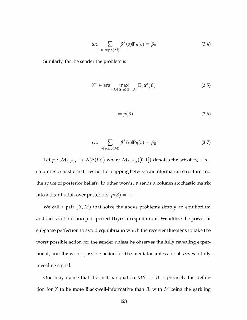
s.t. ∑s∈supp(M)

βR(s)PB(e) = β0 (3.4)

Similarly, for the sender the problem is

X∗ ∈ arg maxX∈X|MX=B

EτuS(β) (3.5)

τ = p(B) (3.6)

s.t. ∑s∈supp(M)

βR(s)PB(e) = β0 (3.7)

Let p : MnS,nΩ → ∆(∆(Ω)) where MnS,nΩ([0, 1]) denotes the set of nS × nΩ

column-stochastic matrices be the mapping between an information structure and

the space of posterior beliefs. In other words, p sends a column stochastic matrix

into a distribution over posteriors: p(B) = τ.

We call a pair (X, M) that solve the above problems simply an equilibrium

and our solution concept is perfect Bayesian equilibrium. We utilize the power of

subgame perfection to avoid equilibria in which the receiver threatens to take the

worst possible action for the sender unless he observes the fully revealing exper-

iment, and the worst possible action for the mediator unless he observes a fully

revealing signal.

One may notice that the matrix equation MX = B is precisely the defini-

tion for X to be more Blackwell-informative than B, with M being the garbling

128

matrix. We will rely on this fact (as well as the different and related implica-

tions of this fact) throughout what is to follow. One can make the simple ob-

servation that the set of Blackwell-ranked information structures forms a chain

when viewed as a subset of the set of all information structures. In addition, we

can also leverage the characterization of the solution in terms of a concavifica-

tion of utility functions, a result that plays a key role in Aumann and Maschler

(1995), Kamenica and Gentzkow (2011) and Gentzkow and Kamenica (2017). Let

Ui(β) , supz|(z, β) ∈ co(ui) where co( f ) denotes the convex hull of the graph

of a function f be the concavification of u. Also define a constrained concavification:

Ui(β|A) , supz|(z, β) ∈ co(vi), β ∈ supp(τ), τ = p(A).

The following version of a lemma from KG will apply:

Lemma 3.2.1 (Kamenica and Gentzkow (2011)). For any final receiver belief β, ui(β) =

Ui(β) if and only if Eτ(ui(β ′)) ≤ ui(β) for all τ such that Eτ(β ′) = β0.

At this level of generality there isn’t anything more to be said about this prob-

lem - it is too general, and likely, intractable.

Given a particular choice of X by the sender, the mediator effectively chooses

from a set of information structures that are Blackwell-dominated by the experi-

ment.

Definition 10. A belief β such that ui(β) = Ui(β) is said to be coincident for player i.

Definition 11. A belief β such that ui(β) = Ui(β), ∀β ∈ C is said to be coincident over

C for player i.

129

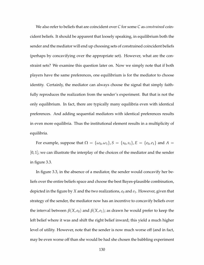
We also refer to beliefs that are coincident over C for some C as constrained coin-

cident beliefs. It should be apparent that loosely speaking, in equilibrium both the

sender and the mediator will end up choosing sets of constrained coincident beliefs

(perhaps by concavifying over the appropriate set). However, what are the con-

straint sets? We examine this question later on. Now we simply note that if both

players have the same preferences, one equilibrium is for the mediator to choose

identity. Certainly, the mediator can always choose the signal that simply faith-

fully reproduces the realization from the sender’s experiment. But that is not the

only equilibrium. In fact, there are typically many equilibria even with identical

preferences. And adding sequential mediators with identical preferences results

in even more equilibria. Thus the institutional element results in a multiplicity of

equilibria.

For example, suppose that Ω = ω0, ω1, S = s0, s1, E = e0, e1 and A =

[0, 1]; we can illustrate the interplay of the choices of the mediator and the sender

in figure 3.3.

In figure 3.3, in the absence of a mediator, the sender would concavify her be-

liefs over the entire beliefs space and choose the best Bayes-plausible combination,

depicted in the figure by X and the two realizations, e0 and e1. However, given that

strategy of the sender, the mediator now has an incentive to concavify beliefs over

the interval between β(X, e0) and β(X, e1); as drawn he would prefer to keep the

left belief where it was and shift the right belief inward; this yield a much higher

level of utility. However, note that the sender is now much worse off (and in fact,

may be even worse off than she would be had she chosen the babbling experiment

130

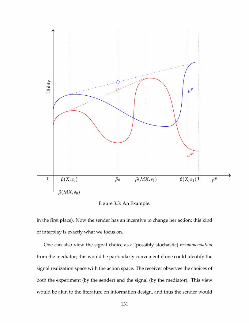
βR10 β0β(X, e0)=

β(MX, s0)

β(X, e1)β(MX, s1)

uS

uM

Uti

lity

Figure 3.3: An Example.

in the first place). Now the sender has an incentive to change her action; this kind

of interplay is exactly what we focus on.

One can also view the signal choice as a (possibly stochastic) recommendation

from the mediator; this would be particularly convenient if one could identify the

signal realization space with the action space. The receiver observes the choices of

both the experiment (by the sender) and the signal (by the mediator). This view

would be akin to the literature on information design, and thus the sender would

131

be designing an experiment subject to an obedience requirement. This however, is

somewhat different from our setting.

For now we focus on the case of a single mediator, as it’s the simplest, builds

intuition and corresponds most closely with the motivating example.

Building Intuition: A Benchmark With BP Utilities

One useful illustration of the present model is to compare the outcomes of a partic-

ular case of the mediated persuasion model to the leading example of the Bayesian

persuasion model presented in KG; doing so also provides a good benchmark for

the possible outcomes and builds intuition. To that end, suppose that we take

the simple model presented in KG, keep the preferences the same and the add a

mediator. Ω = guilty, innocent, E = S = g, i and A = convict, acquit,

uS(a) =

1 if aR = convict

0 otherwise

(3.8)

and

uR(a, ω) =

1 if ω = guilty & aR = convict

1 if ω = innocent & aR = acquit

0 otherwise

(3.9)

Suppose that the common prior belief of ω = guilty is β0 = 0.3. We are left of

course, with the question of what the preferences of the mediator are; one of our

132

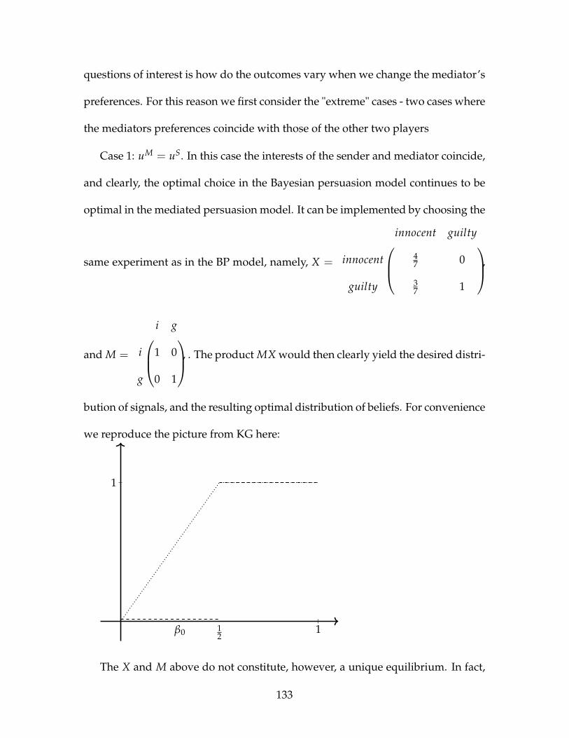
questions of interest is how do the outcomes vary when we change the mediator’s

preferences. For this reason we first consider the "extreme" cases - two cases where

the mediators preferences coincide with those of the other two players

Case 1: uM = uS. In this case the interests of the sender and mediator coincide,

and clearly, the optimal choice in the Bayesian persuasion model continues to be

optimal in the mediated persuasion model. It can be implemented by choosing the

same experiment as in the BP model, namely, X =

innocent guiltyinnocent 4

7 0

guilty 37 1

,

and M =

i gi 1 0

g 0 1

, . The product MX would then clearly yield the desired distri-

bution of signals, and the resulting optimal distribution of beliefs. For convenience

we reproduce the picture from KG here:

β0 12

1

1

The X and M above do not constitute, however, a unique equilibrium. In fact,

133

any pair (M, X) with the property that their product results in a Bayes-plausible

combination of the beliefs β = 0 and β = 0.5 is an equilibrium. This simple

example shows that the mere presence of a mediator can increase the number of

equilibria, but keep the outcome the same.

Case 2: uM = uR. We now turn to the question of what happens if the me-

diator’s preferences are fully aligned with those of the receiver. While intuition

suggests that this arrangement is must be better for the receiver, we show by ex-

ample that in fact, this does not have to be strictly so. Writing the mediator’s utility

as a function of the receiver’s belief we obtain

uM(β) =

1− β if β < 1

2

β if β ≥ 12

which we plot on the graph below in red.

β0 12

1

1

12

The concavification of uM over the entire belief space (which we do not depict)

is simply a straight line at 1. If the sender induces the same two beliefs (β = 0 and

β = 0.5) as in the base case, since any garbling of these two beliefs would induce

134

beliefs that are interior to the set [0, 0.5] and since the mediator’s utility is linear

in the subset of belief space that is feasible (and therefore the constrained concav-

ification coincides with utility everywhere), the mediator is indifferent between

any Bayes-plausible garbling of the two beliefs. As for the sender, she gets zero

utility from any beliefs β ∈ [0, 12). Since the mediator is indifferent over the space

of constrained beliefs, in particular, the original equilibrium outcome can be sus-

tained in the same way as above - the sender plays X and the mediator truthfully

reproduces the experiment realization.

Observe however, that if the mediator were to play any nontrivial garbling,

that would not be an equilibrium, since then the sender would get utility zero (as

opposed to getting 0.6 in equilibrium), and would have an incentive to "undo"

the garbling, bringing the beliefs back outward. Additionally, it is also not an

equilibrium for the sender to play something that is strictly more informative than

X, since then one of the beliefs would be above 12 , in which case the mediator’s

utility would be convex over the set of possible posterior beliefs, and the mediator

would have a strict incentive to play a fully revealing M, in which case the sender

would prefer to deviate back to X.

Suppose that the sender chooses a particular experiment X and the mediator

chooses a particular experiment M. Observe that then the receiver is computing

the posterior belief from a combined distribution that is simply the product of the

two choices: MX , B. Since M is a column-stochastic matrix, as noted above, this

is precisely the definition of B being Blackwell-inferior (Blackwell (1951), Black-

well (1953)) to X with M being the garbling matrix. Thus, whatever the mediator

135

chooses, the resulting distribution of signal realizations will be dominated by the

sender’s experiment in the sense of Blackwell. Blackwell’s characterizations imme-

diately apply and we have the following series of results which we state without

proof since they are direct consequences of Blackwell’s theorem.

Observation 2. The distribution of receiver beliefs under X is a mean-preserving spread

of the distribution of receiver beliefs under B.

If the sender and the mediator have the same preferences, full revelation may

not be an equilibrium (in that case the set of equilibrium outcomes coincides with

that in KG). In Gentzkow and Kamenica (2017a) and Gentzkow and Kamenica

(2017b) full revelation is typically an equilibrium (with at least two senders); the

reason is that they identify a condition on the informational environment ("Blackwell-

connectedness") which guarantees that each player can unilaterally deviate to a

Blackwell-more informative outcome, regardless of the actions of the other player.

Preference divergence then forces full revelation. Finally, adding senders does not

make the uninformative equilibrium disappear.

3.3 Binary Model

For tractability we work with a binary model where there are two states of the

world and two experiment and signal realizations. This is with (perhaps signif-

icant) loss of generality, but will serve well to illustrate the basic idea of how to

compute a best response for the sender given the choice of the mediator.

136

Computing the Set of Feasible Posteriors

Setting aside the issues of strategic behavior for now, we first ask a simpler ques-

tion: given a fixed9 signal (or equivalently, a fixed garbling), or a fixed experiment,

what are all the posterior distributions that can be induced? At this point we can

make an important connection with the cheap talk and communication literature.

Blume, Board and Kawamura (2007) discuss a model of cheap talk where the signal

sent by the sender is subject to random error - with a small probability the message

observed by the receiver is not the message sent by the sender, but rather, a mes-

sage sent from some other distribution that does not depend on the sender’s type

or the message chosen. We make this connection to note that choosing an informa-

tion structure that will be subjected to a fixed, non-strategically-chosen garbling is

exactly equivalent to choosing a random signal that will be subject to noise. Thus,

our model subsumes a model on Bayesian persuasion with noisy communication.

In the (different but related) setting of cheap talk, as noted by Ambrus, Azevedo

and Kamada (2013) as well as Blume, Board and Kawamura (2007) stochastic re-

ports make incentive compatibility constraints easier to satisfy. This will not quite

be the case here, but this will nevertheless be an illuminating exercise.

As mentioned above, for tractability10 we will work in the simplest possible en-

vironment of binary signal and state spaces for both the sender and the mediator.

In addition to being the simplest nontrivial example of the problem we are trying

to solve, working with two-by-two square matrices has a very important addi-

9I.e. not strategically chosen by a player as a function of her preferences.10And with loss of generality, which we discuss later.

137

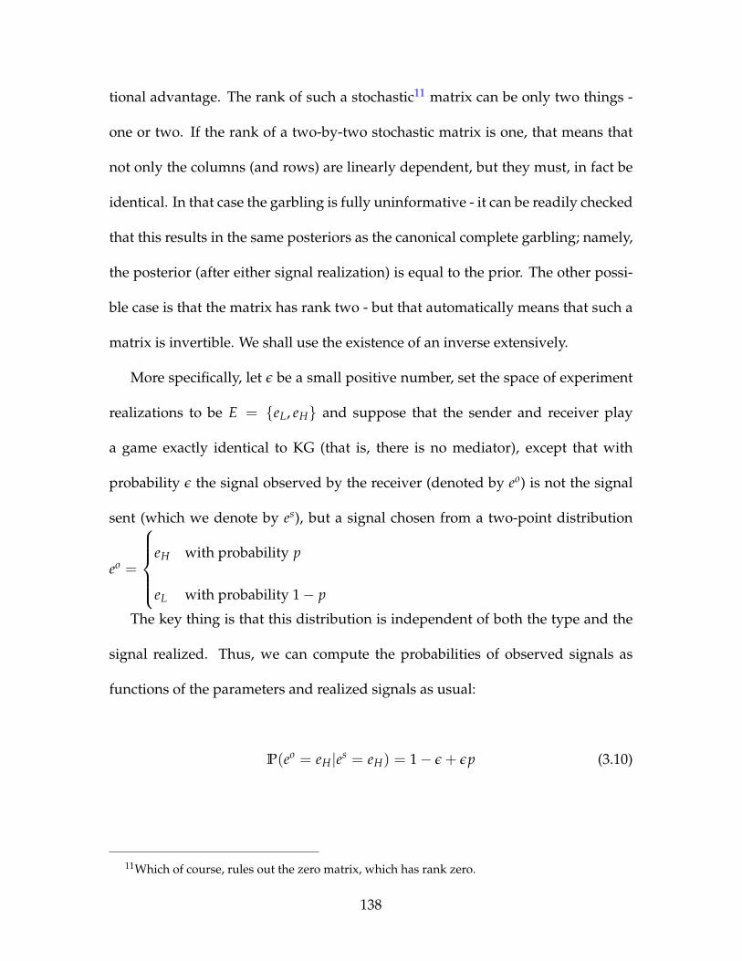
tional advantage. The rank of such a stochastic11 matrix can be only two things -

one or two. If the rank of a two-by-two stochastic matrix is one, that means that

not only the columns (and rows) are linearly dependent, but they must, in fact be

identical. In that case the garbling is fully uninformative - it can be readily checked

that this results in the same posteriors as the canonical complete garbling; namely,

the posterior (after either signal realization) is equal to the prior. The other possi-

ble case is that the matrix has rank two - but that automatically means that such a

matrix is invertible. We shall use the existence of an inverse extensively.

More specifically, let ε be a small positive number, set the space of experiment

realizations to be E = eL, eH and suppose that the sender and receiver play

a game exactly identical to KG (that is, there is no mediator), except that with

probability ε the signal observed by the receiver (denoted by eo) is not the signal

sent (which we denote by es), but a signal chosen from a two-point distribution

eo =

eH with probability p

eL with probability 1− p

The key thing is that this distribution is independent of both the type and the

signal realized. Thus, we can compute the probabilities of observed signals as

functions of the parameters and realized signals as usual:

P(eo = eH|es = eH) = 1− ε + εp (3.10)

11Which of course, rules out the zero matrix, which has rank zero.

138

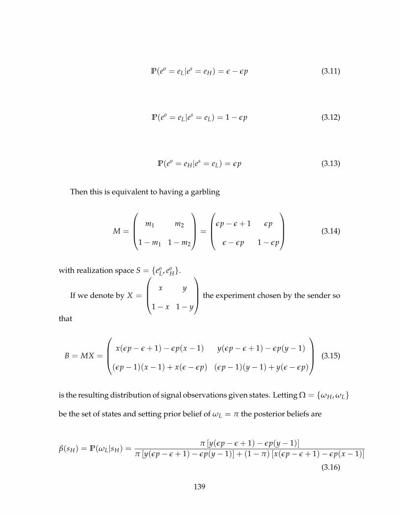
P(eo = eL|es = eH) = ε− εp (3.11)

P(eo = eL|es = eL) = 1− εp (3.12)

P(eo = eH|es = eL) = εp (3.13)

Then this is equivalent to having a garbling

M =

m1 m2

1−m1 1−m2

=

εp− ε + 1 εp

ε− εp 1− εp

(3.14)

with realization space S = eoL, eo

H.

If we denote by X =

x y

1− x 1− y

the experiment chosen by the sender so

that

B = MX =

x(εp− ε + 1)− εp(x− 1) y(εp− ε + 1)− εp(y− 1)

(εp− 1)(x− 1) + x(ε− εp) (εp− 1)(y− 1) + y(ε− εp)

(3.15)

is the resulting distribution of signal observations given states. Letting Ω = ωH, ωL

be the set of states and setting prior belief of ωL = π the posterior beliefs are

β(sH) = P(ωL|sH) =π [y(εp− ε + 1)− εp(y− 1)]

π [y(εp− ε + 1)− εp(y− 1)] + (1− π) [x(εp− ε + 1)− εp(x− 1)]

(3.16)

139

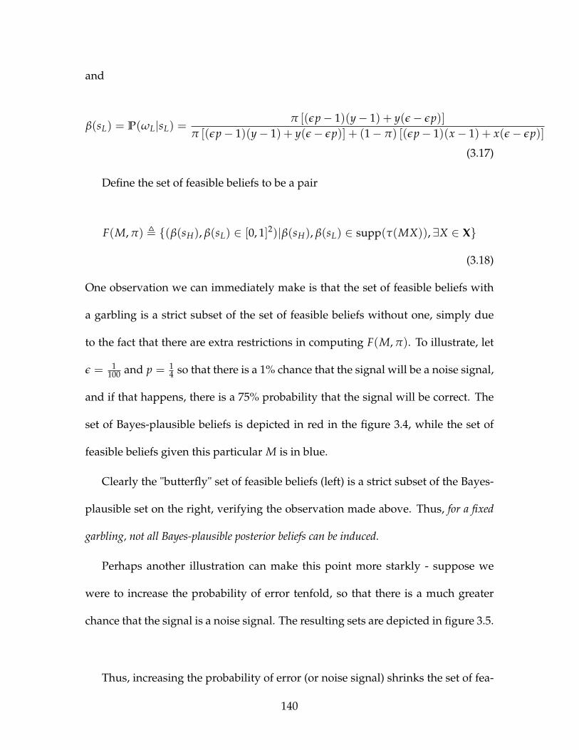
and

β(sL) = P(ωL|sL) =π [(εp− 1)(y− 1) + y(ε− εp)]

π [(εp− 1)(y− 1) + y(ε− εp)] + (1− π) [(εp− 1)(x− 1) + x(ε− εp)]

(3.17)

Define the set of feasible beliefs to be a pair

F(M, π) , (β(sH), β(sL) ∈ [0, 1]2)|β(sH), β(sL) ∈ supp(τ(MX)), ∃X ∈ X

(3.18)

One observation we can immediately make is that the set of feasible beliefs with

a garbling is a strict subset of the set of feasible beliefs without one, simply due

to the fact that there are extra restrictions in computing F(M, π). To illustrate, let

ε = 1100 and p = 1

4 so that there is a 1% chance that the signal will be a noise signal,

and if that happens, there is a 75% probability that the signal will be correct. The

set of Bayes-plausible beliefs is depicted in red in the figure 3.4, while the set of

feasible beliefs given this particular M is in blue.

Clearly the "butterfly" set of feasible beliefs (left) is a strict subset of the Bayes-

plausible set on the right, verifying the observation made above. Thus, for a fixed

garbling, not all Bayes-plausible posterior beliefs can be induced.

Perhaps another illustration can make this point more starkly - suppose we

were to increase the probability of error tenfold, so that there is a much greater

chance that the signal is a noise signal. The resulting sets are depicted in figure 3.5.

Thus, increasing the probability of error (or noise signal) shrinks the set of fea-

140

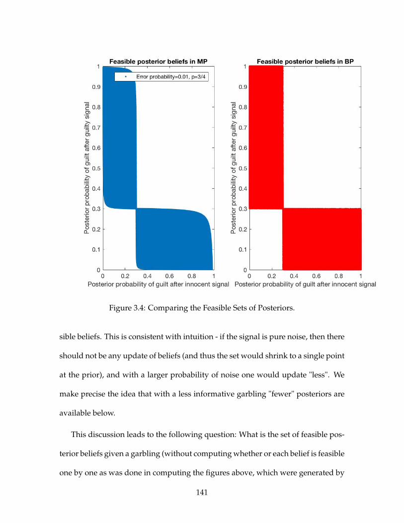
Figure 3.4: Comparing the Feasible Sets of Posteriors.

sible beliefs. This is consistent with intuition - if the signal is pure noise, then there

should not be any update of beliefs (and thus the set would shrink to a single point

at the prior), and with a larger probability of noise one would update "less". We

make precise the idea that with a less informative garbling "fewer" posteriors are

available below.

This discussion leads to the following question: What is the set of feasible pos-

terior beliefs given a garbling (without computing whether or each belief is feasible

one by one as was done in computing the figures above, which were generated by

141

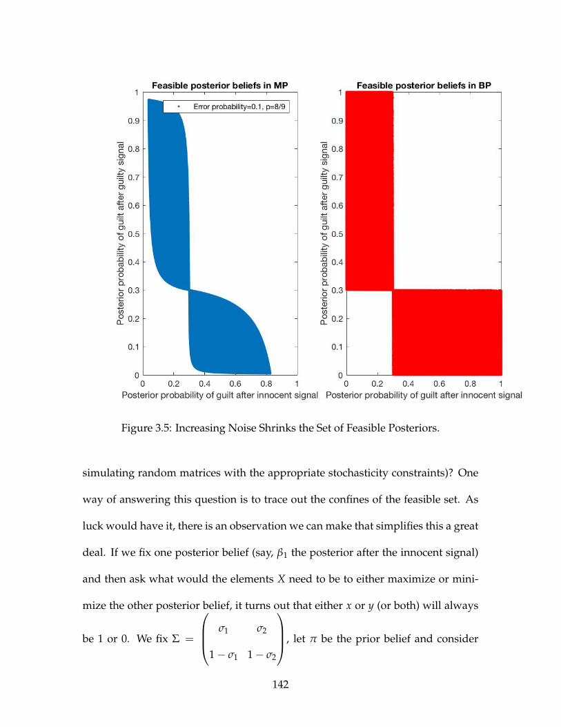
Figure 3.5: Increasing Noise Shrinks the Set of Feasible Posteriors.

simulating random matrices with the appropriate stochasticity constraints)? One

way of answering this question is to trace out the confines of the feasible set. As

luck would have it, there is an observation we can make that simplifies this a great

deal. If we fix one posterior belief (say, β1 the posterior after the innocent signal)

and then ask what would the elements X need to be to either maximize or mini-

mize the other posterior belief, it turns out that either x or y (or both) will always

be 1 or 0. We fix Σ =

σ1 σ2

1− σ1 1− σ2

, let π be the prior belief and consider

142

X =

x y

1− x 1− y

. Computing outer limits of F(Σ, π) is equivalent to the fol-

lowing program:

maxx,y

β2 =π[σ1y + σ2(y− 1)]

π[σ1y + σ2(y− 1)] + (1− π)[σ1x− σ2(x− 1)](3.19)

s.t. β1 = const. (3.20)

0 ≤ x ≤ 1; 0 ≤ y ≤ 1 (3.21)

The solution shows that either x, or y or both will be 0 or 1 (and of course, we

could also have fixed β2 and let that be the parameter; the answer would be the

same). The result is intuitive (maximizing a posterior belief requires maximizing

the probability of one of the signals in the first place), but this verifies the intuition.

Again, fortunately for us, this observation can be operationalized in the fol-

lowing way: we first fix one of four extreme points of the X matrix, and then trace

out the corresponding possible beliefs by systematically varying the other prob-

abilities in the experiment, which yields a curve (or a path, in topological terms)

parametrized by a single number - the probability of one of the signals.

We illustrate this approach using M =

13

17

23

67

. The question is, what is

F(M, π) for this garbling? We use the algorithm just prescribed: first fix a perfectly

revealing part of the experiment, and then vary the corresponding distribution.

143

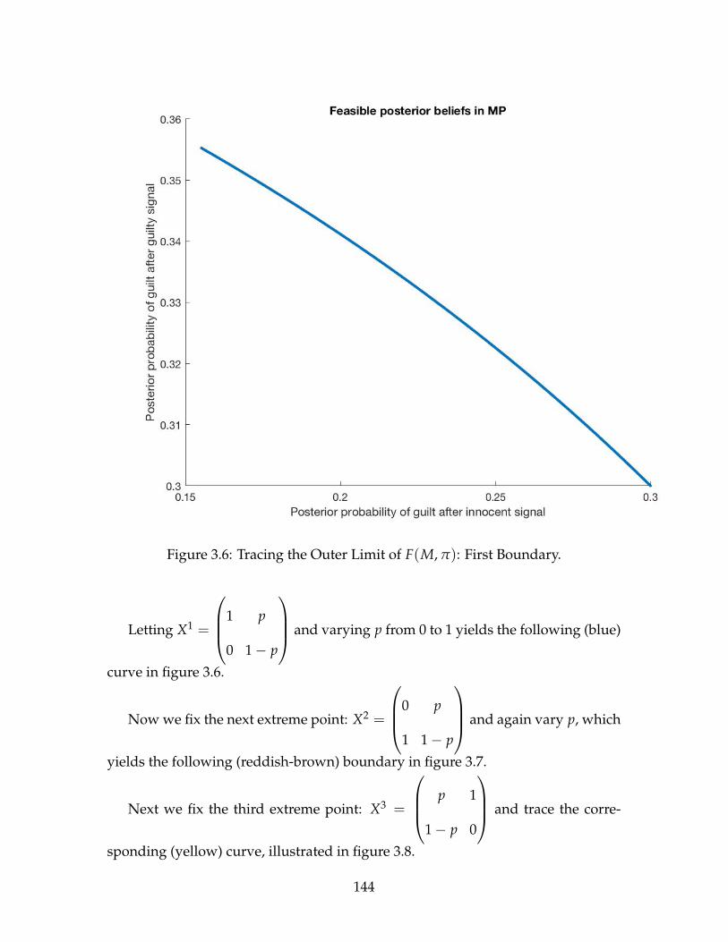
Figure 3.6: Tracing the Outer Limit of F(M, π): First Boundary.

Letting X1 =

1 p

0 1− p

and varying p from 0 to 1 yields the following (blue)

curve in figure 3.6.

Now we fix the next extreme point: X2 =

0 p

1 1− p

and again vary p, which

yields the following (reddish-brown) boundary in figure 3.7.

Next we fix the third extreme point: X3 =

p 1

1− p 0

and trace the corre-

sponding (yellow) curve, illustrated in figure 3.8.

144

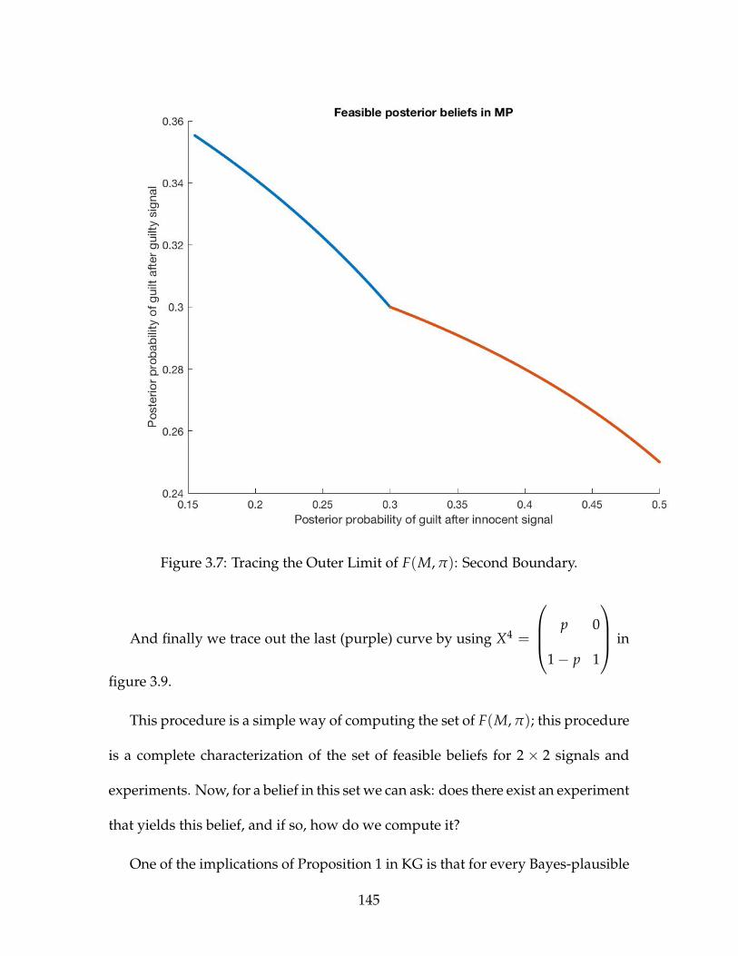
Figure 3.7: Tracing the Outer Limit of F(M, π): Second Boundary.

And finally we trace out the last (purple) curve by using X4 =

p 0

1− p 1

in

figure 3.9.

This procedure is a simple way of computing the set of F(M, π); this procedure

is a complete characterization of the set of feasible beliefs for 2 × 2 signals and

experiments. Now, for a belief in this set we can ask: does there exist an experiment

that yields this belief, and if so, how do we compute it?

One of the implications of Proposition 1 in KG is that for every Bayes-plausible

145

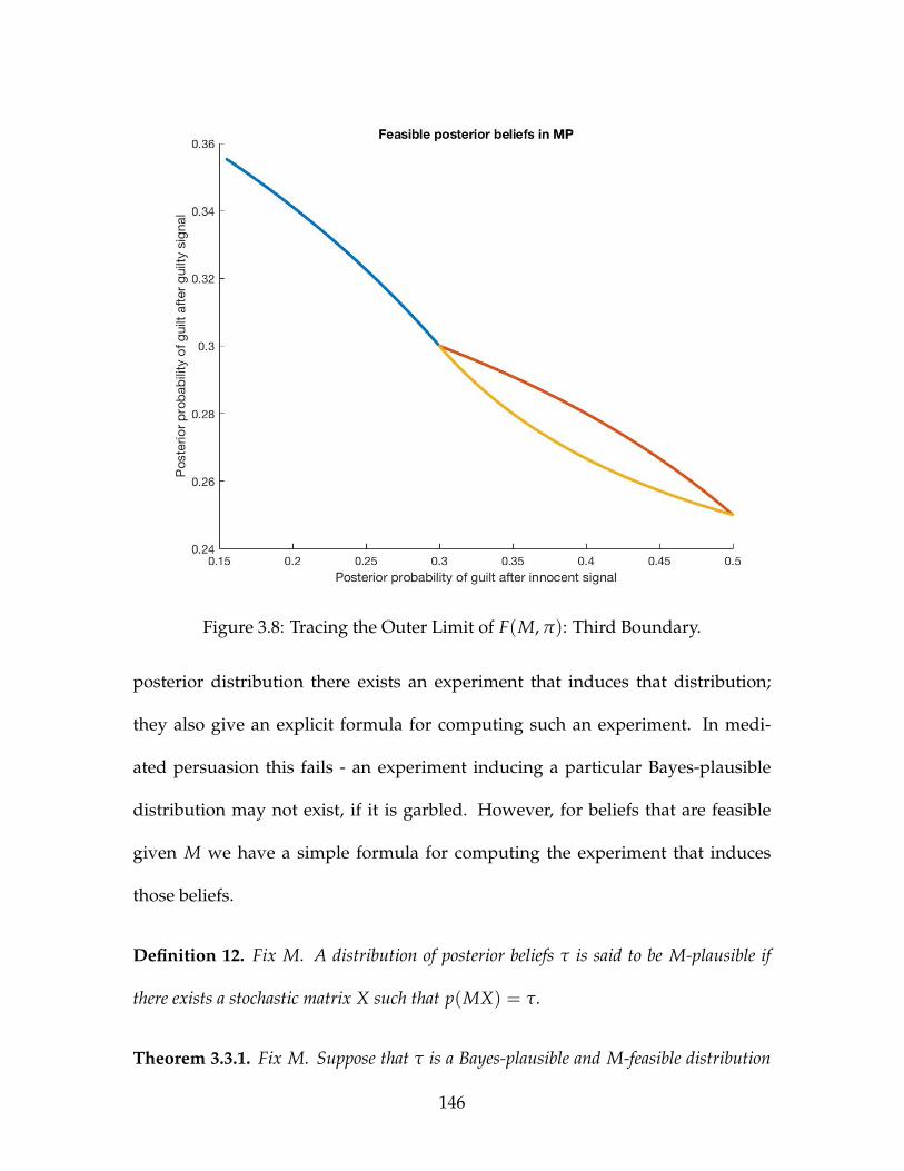
Figure 3.8: Tracing the Outer Limit of F(M, π): Third Boundary.

posterior distribution there exists an experiment that induces that distribution;

they also give an explicit formula for computing such an experiment. In medi-

ated persuasion this fails - an experiment inducing a particular Bayes-plausible

distribution may not exist, if it is garbled. However, for beliefs that are feasible

given M we have a simple formula for computing the experiment that induces

those beliefs.

Definition 12. Fix M. A distribution of posterior beliefs τ is said to be M-plausible if

there exists a stochastic matrix X such that p(MX) = τ.

Theorem 3.3.1. Fix M. Suppose that τ is a Bayes-plausible and M-feasible distribution

146

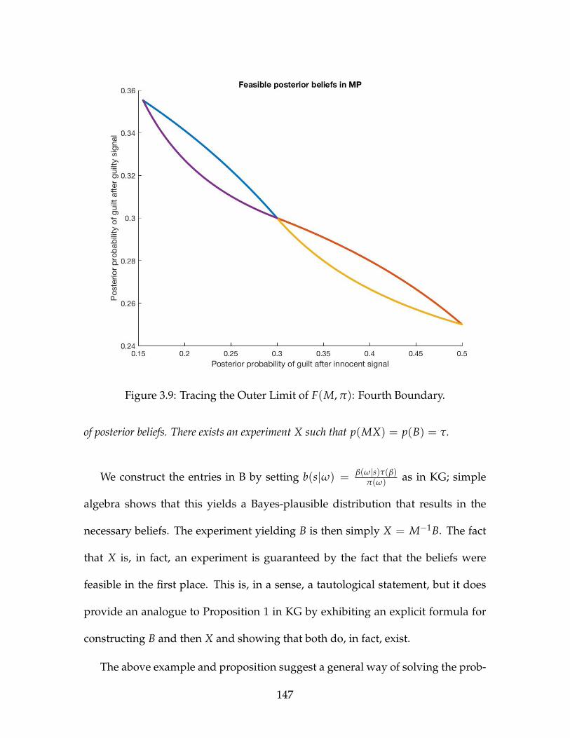
Figure 3.9: Tracing the Outer Limit of F(M, π): Fourth Boundary.

of posterior beliefs. There exists an experiment X such that p(MX) = p(B) = τ.

We construct the entries in B by setting b(s|ω) = β(ω|s)τ(β)π(ω)

as in KG; simple

algebra shows that this yields a Bayes-plausible distribution that results in the

necessary beliefs. The experiment yielding B is then simply X = M−1B. The fact

that X is, in fact, an experiment is guaranteed by the fact that the beliefs were

feasible in the first place. This is, in a sense, a tautological statement, but it does

provide an analogue to Proposition 1 in KG by exhibiting an explicit formula for

constructing B and then X and showing that both do, in fact, exist.

The above example and proposition suggest a general way of solving the prob-

147

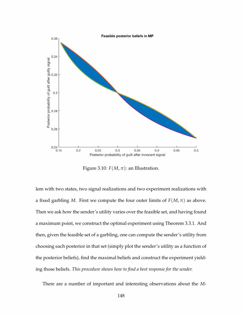
Figure 3.10: F(M, π): an Illustration.

lem with two states, two signal realizations and two experiment realizations with

a fixed garbling M. First we compute the four outer limits of F(M, π) as above.

Then we ask how the sender’s utility varies over the feasible set, and having found

a maximum point, we construct the optimal experiment using Theorem 3.3.1. And

then, given the feasible set of a garbling, one can compute the sender’s utility from

choosing each posterior in that set (simply plot the sender’s utility as a function of

the posterior beliefs), find the maximal beliefs and construct the experiment yield-

ing those beliefs. This procedure shows how to find a best response for the sender.

There are a number of important and interesting observations about the M-

148

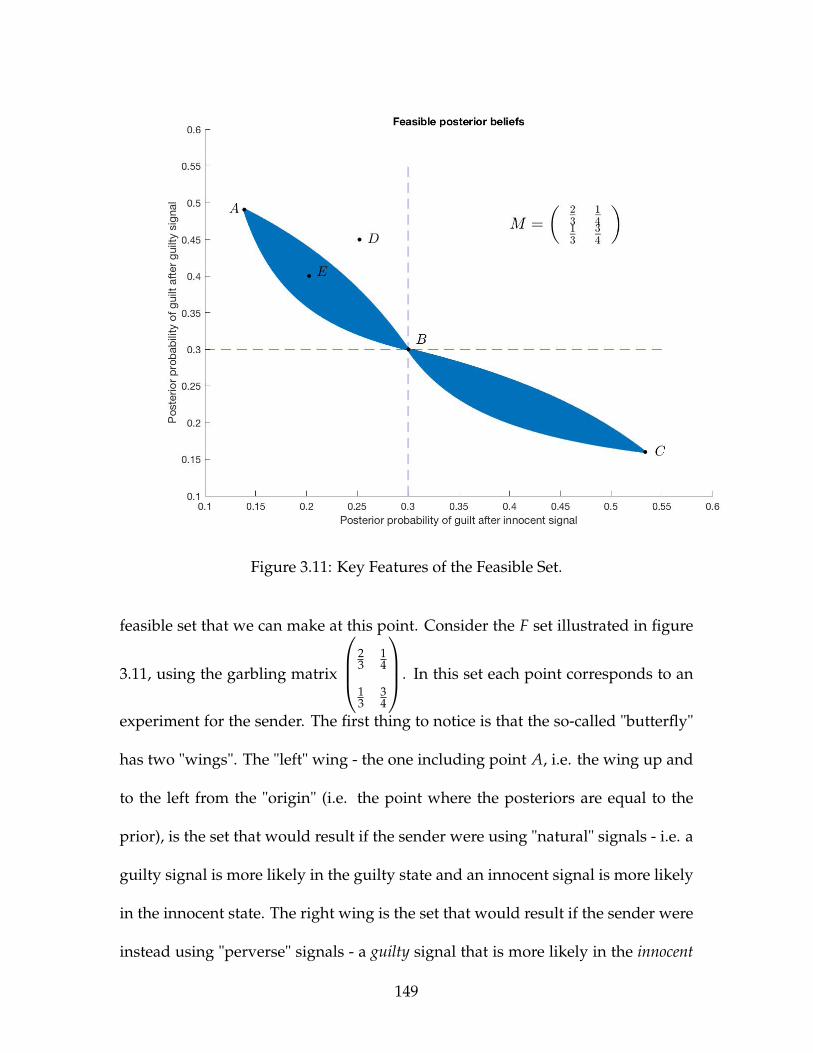
Figure 3.11: Key Features of the Feasible Set.

feasible set that we can make at this point. Consider the F set illustrated in figure

3.11, using the garbling matrix

23

14

13

34

. In this set each point corresponds to an

experiment for the sender. The first thing to notice is that the so-called "butterfly"

has two "wings". The "left" wing - the one including point A, i.e. the wing up and

to the left from the "origin" (i.e. the point where the posteriors are equal to the

prior), is the set that would result if the sender were using "natural" signals - i.e. a

guilty signal is more likely in the guilty state and an innocent signal is more likely

in the innocent state. The right wing is the set that would result if the sender were

instead using "perverse" signals - a guilty signal that is more likely in the innocent

149

state, and vice versa12. This is also equivalent to flipping the labels on the signals.

Consider point B, the point where both posteriors are equal to the prior (with

the obvious motivation, we call that the "origin"). Observe that moving weakly

northwest meaning decreasing the first posterior while increasing the second - in

other words, a mean-preserving spread13. Thus, points that are northwest of B are

posteriors that are Blackwell-more informative than B. Equivalently, they corre-

spond to signals that Blackwell dominate the uninformative signals. Iterating this,

point A is Blackwell-most informative among all the points in the left wing. It can

also be verified that point A is precisely the two posteriors that correspond to the

sender using the fully informative (and "natural") signal. The exact opposite logic

applies to the right wing, so that C is the extreme posterior corresponding to the

Blackwell-most informative "perverse" signal. Importantly, this logic works only

within each wing, (or quadrant by quadrant, which are delineated by the dashed

lines), and not on the figure as a whole.

The other observation that we can make is that while F seems symmetric around

the "origin", in general, it is not. The lack of symmetry comes from the constraints

(and biases) imparted by the garbling; F(M, π) is symmetric if and only if M is

symmetric.

Definition 13. F is said to be symmetric if for each β1, β2 if the ordered pair β1, β2 ∈

F then the ordered pair β2, β1 is also in F.

12Note that if the sender were to choose a signal, say, guilty, that is more likely in both states,that would quickly bring beliefs back to the prior, and whether it would be in the right or the leftwing would be dictated by the relative probabilities.

13The fact that the spread is mean preserving comes from Bayes rule.

150

The next observation is that each wing of the butterfly is convex, but the but-

terfly itself is not. This comes from the fact that for normal (and respectively, for

perverse) signals, if two posteriors can be induced, than so can any convex com-

bination (since the set of the relevant stochastic matrices is convex). On the other

hand, for the entire set to be convex, taking a point from the left wing, a point from

the right and requiring that a mixture would also be in the set would require each

signal to be weakly more likely in either state - which is impossible, except for the

degenerate case. This is why we can take the convex hull of the extreme beliefs

and outer limits for each wing, but not the convex hull of the entire butterfly.

The final observation that we can make is the following: the sender is certainly

capable of choosing the identity experiment, and inducing MI = B (in figure 3.11

this would correspond to point A); this is the best (in the sense of being Blackwell-

maximal) that the sender can induce. Since the sender can also choose any less

informative experiment, it would seem that the sender may be capable of inducing

any Blackwell-inferior distribution to A. Figure 3.11 shows that this intuition is

false. A point like D is certainly Blackwell-inferior to A, being a mean-preserving

contraction, yet it is outside the feasible set. The question then arises, why can we

not simply "construct" the required experiment X as follows: suppose MI B ′

and p(B ′) = D. If there exists an X with MX = B ′, we would be done. What

about simply putting X = M−1B ′? The answer is that if p(MM−1B ′) is in F,

this would work. It turns out that if that it not true, then M−1B ′ will not yield a

stochastic matrix X and therefore would not be a valid experiment (this can be seen

by example). In other words, the sender is not capable of inducing any posterior

151

belief that is Blackwell-inferior to MI.

There are a number of interesting results that we can illustrate using this tech-

nique of considering the feasible sets. For example,

Theorem 3.3.2. Suppose M1 and M2 are two garblings with M1 B M2. Then F(M2, π) ⊆

F(M1, π).

Proof. Fix any π. We must show that for any τ if supp(τ) ∈ F(M2, π), then

supp(τ) ∈ F(M1, π).By assumption we have that p(M2X) = τ for some X. The

question is, does there exist a Y such that τ = p(M1Y)? In other words, does there

exist a Y such that M2X = M1Y? The answer is yes; by assumption we have that

ΓM1 = M2 for some Γ. Thus,

M2X = M1Y ⇒ ΓM1X = M1Y (3.22)

and therefore the required Y is given by

Y = M−11 ΓM1X (3.23)

Note that Y does depend on both M1 and X, as intuition would suggest.

In other words, using a strictly more Blackwell-informative garbling results

in a strictly larger set of feasible receiver posterior beliefs. Of course, this is ob-

vious with trivial garblings (an identity, which would leave the feasible set un-

changed from the Bayes-plausible one, and a completely uninformative garbling

152

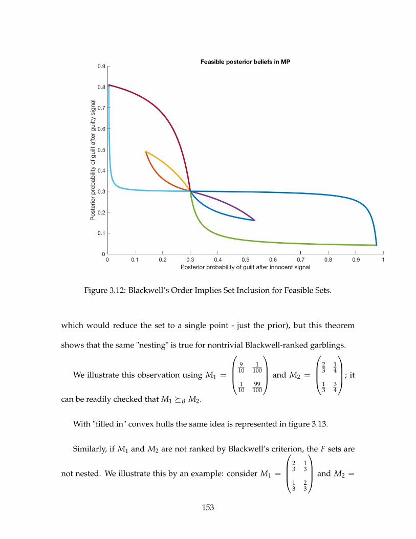
Figure 3.12: Blackwell’s Order Implies Set Inclusion for Feasible Sets.

which would reduce the set to a single point - just the prior), but this theorem

shows that the same "nesting" is true for nontrivial Blackwell-ranked garblings.

We illustrate this observation using M1 =

910

1100

110

99100

and M2 =

23

14

13

34

; it

can be readily checked that M1 B M2.

With "filled in" convex hulls the same idea is represented in figure 3.13.

Similarly, if M1 and M2 are not ranked by Blackwell’s criterion, the F sets are

not nested. We illustrate this by an example: consider M1 =

23

13

13

23

and M2 =

153

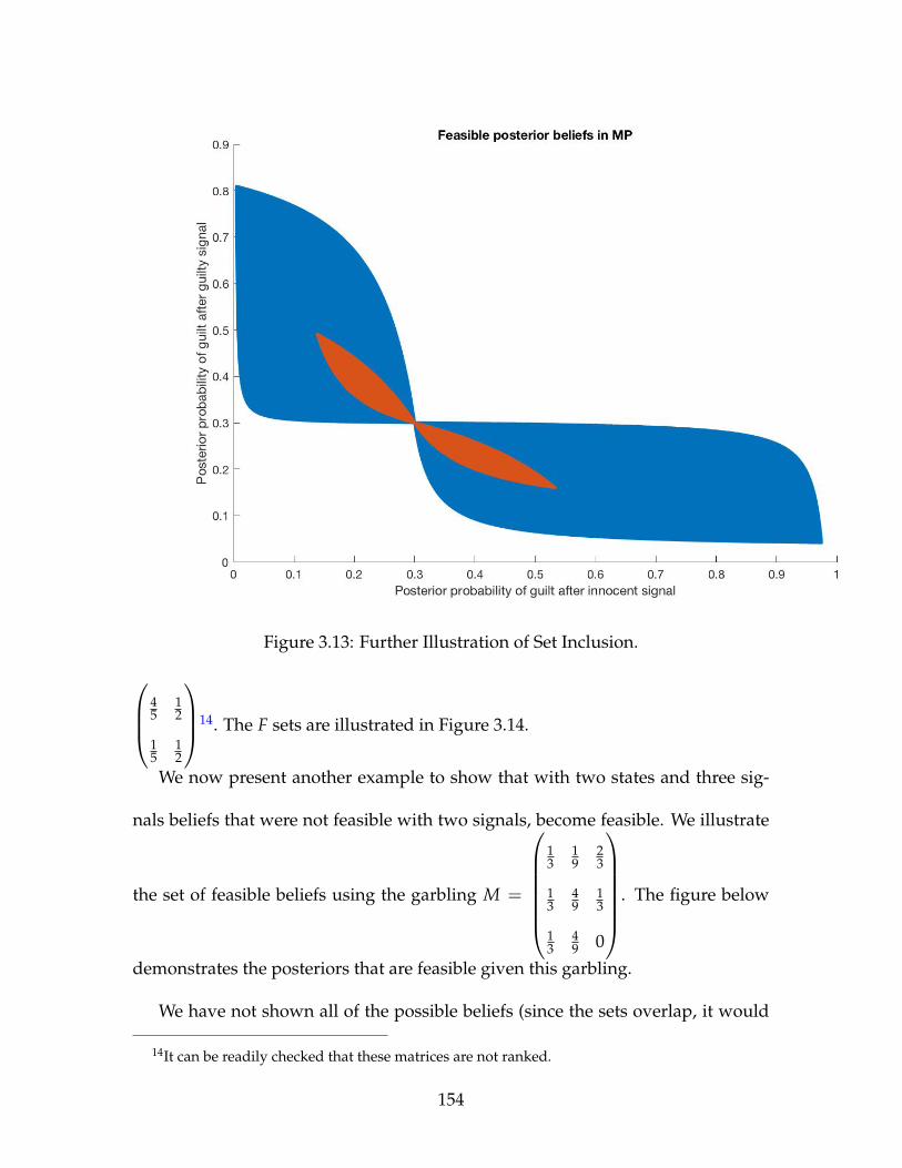
Figure 3.13: Further Illustration of Set Inclusion.

45

12

15

12

14. The F sets are illustrated in Figure 3.14.

We now present another example to show that with two states and three sig-

nals beliefs that were not feasible with two signals, become feasible. We illustrate

the set of feasible beliefs using the garbling M =

13

19

23

13

49

13

13

49 0

. The figure below

demonstrates the posteriors that are feasible given this garbling.

We have not shown all of the possible beliefs (since the sets overlap, it would

14It can be readily checked that these matrices are not ranked.

154

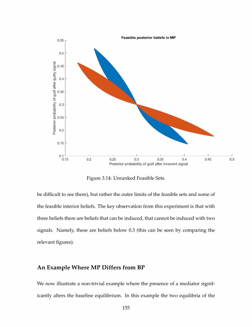
Figure 3.14: Unranked Feasible Sets.

be difficult to see them), but rather the outer limits of the feasible sets and some of

the feasible interior beliefs. The key observation from this experiment is that with

three beliefs there are beliefs that can be induced, that cannot be induced with two

signals. Namely, these are beliefs below 0.3 (this can be seen by comparing the

relevant figures).

An Example Where MP Differs from BP

We now illustrate a non-trivial example where the presence of a mediator signif-

icantly alters the baseline equilibrium. In this example the two equilibria of the

155

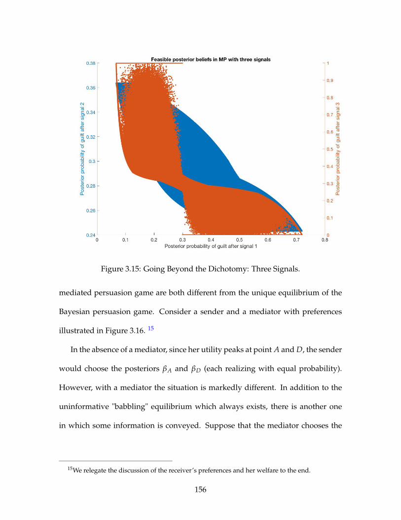
Figure 3.15: Going Beyond the Dichotomy: Three Signals.

mediated persuasion game are both different from the unique equilibrium of the

Bayesian persuasion game. Consider a sender and a mediator with preferences

illustrated in Figure 3.16. 15

In the absence of a mediator, since her utility peaks at point A and D, the sender

would choose the posteriors βA and βD (each realizing with equal probability).

However, with a mediator the situation is markedly different. In addition to the

uninformative "babbling" equilibrium which always exists, there is another one

in which some information is conveyed. Suppose that the mediator chooses the

15We relegate the discussion of the receiver’s preferences and her welfare to the end.

156

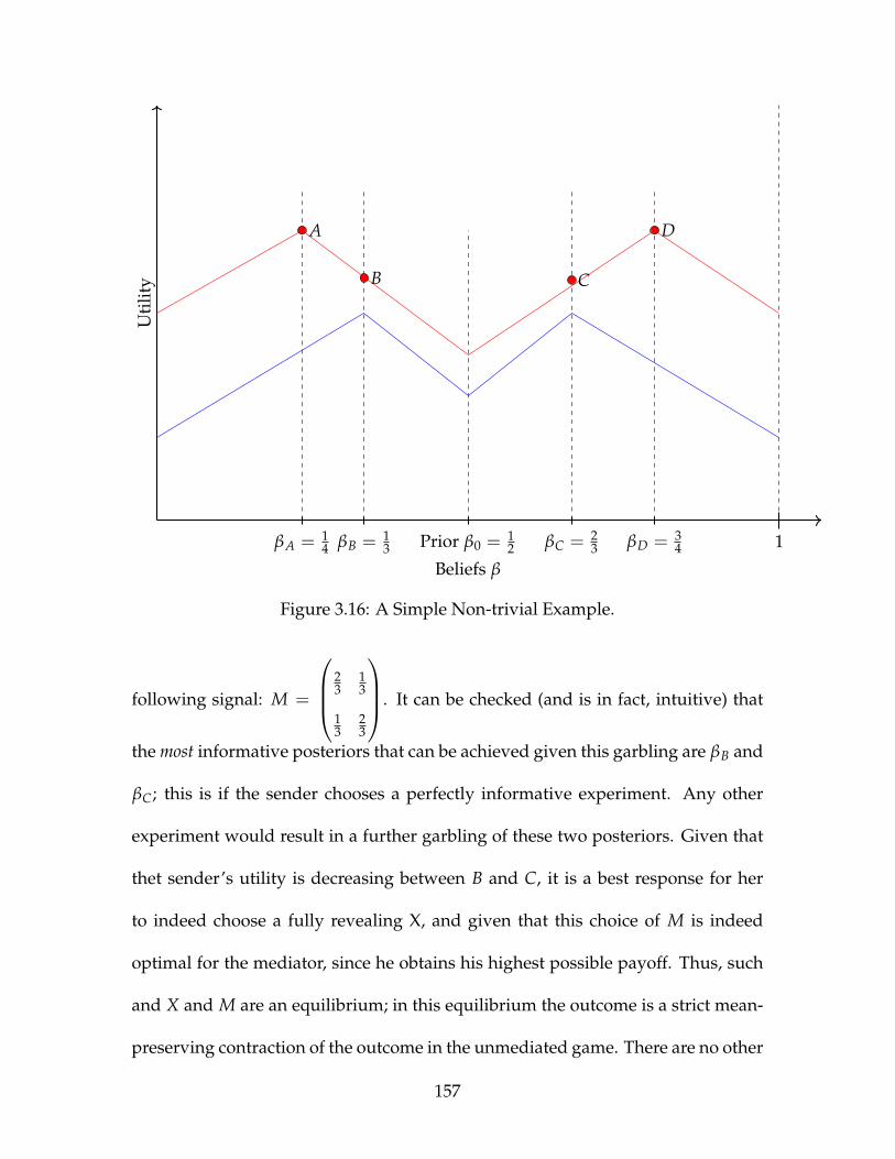
1Prior β0 = 12

Beliefs β

Uti

lity

βA = 14 βD = 3

4βB = 13 βC = 2

3

A

B

D

C

Figure 3.16: A Simple Non-trivial Example.

following signal: M =

23

13

13

23

. It can be checked (and is in fact, intuitive) that

the most informative posteriors that can be achieved given this garbling are βB and

βC; this is if the sender chooses a perfectly informative experiment. Any other

experiment would result in a further garbling of these two posteriors. Given that

thet sender’s utility is decreasing between B and C, it is a best response for her

to indeed choose a fully revealing X, and given that this choice of M is indeed

optimal for the mediator, since he obtains his highest possible payoff. Thus, such

and X and M are an equilibrium; in this equilibrium the outcome is a strict mean-

preserving contraction of the outcome in the unmediated game. There are no other

157

pure strategy equilibria in this game.

We now turn to the question of receiver welfare. It is immediate that if the

receiver’s preferences are the same as those of the mediator, then the receiver is

strictly better off. If, on the other hand, the receiver has preferences that emphasize

certainty of the state (such as the preferences of the receiver in the leading example

of KG, for instance), the receiver is strictly worse off with a mediator. This simple

example illustrates that the presence of the mediator has an ambiguous effect on

the welfare of the receiver.

Interpretation of the Rank of a Garbling Matrix

We now turn to a discussion of one of the key conditions established above - the

necessity for M to be of full rank. This is a fairly straightforward question, yet it

has never come up in the literature - what is the economic interpretation of the

rank of a garbling matrix?

For simplicity suppose that the matrix is square, so that full rank guarantees

invertibility16 We first start with a discussion of what is means for a garbling ma-

trix to not be invertible. By definition of rank, the column rank and the row rank

of a matrix are always identical; recall also the convention that the columns of a

garbling matrix represent signal realizations in each state of the world. If a matrix

is not invertible, it means that there is at least one columns (a profile of signals in

a given state) that is a linear combination of the other columns. In other words,

16We say a few words about non-square matrices below.

158

one can replicate the distribution of signals in a state without knowing anything about

the state. This is literally the definition of a Blackwell garbling.

The corresponding (row) point of view offers the same insight. If a garbling

matrix is not invertible, then the distribution of a particular signal in all possible

states is a linear combination of the distributions of the signals in the other states,

and hence, one can replicate the distribution of a signal. In other words, a singular

garbling contains within itself a sort of Blackwell garbling. Whether or not this

internal garbling can be "undone", perhaps by constructing a new one, remains an

open question17

This discussion sheds some light on the invertibility condition. The fact that the

garblings used in the discussion of the feasible sets were all invertible means that

they carry "as much information as possible", given their dimensional constraints.

Finally, suppose that the garbling is not square, i.e. M is a m-by-n matrix with

m signals, n states and m ≥ n18. The M being full rank means that the rank of

M is equal to n, the number of states, which in turn implies that there always

exists a left inverse. Observe that all of the inverses discussed so far were always

used in left-multiplying the relevant matrices, so for non-square garblings the logic

and algebra of being full rank is the same as the logic of invertibility for square

matrices.

17For example, given a garbling suppose that the receiver constructs another garbling from that,one that has full rank. What are the properties of this artificial garbling relative to the original one?

18Recall that the assumption that there are at least as many signals as states is made to avoidsome trivialities which arise when the signal space is not "rich enough".

159

Modifications

There are a number of fairly obvious modifications to the basic model that can be

made; we summarize these in the present section.

The first has to do with preference misalignment between the sender and the

mediator. It should be clear that the more misaligned (in any reasonable sense) the

preferences are, less information revelation. And in fact, depending on the mea-

sure of misalignment, the informative equilibria "quickly" vanish as misalignment

increases, leaving only the babbling equilibrium.

The second modification is varying the number of mediators; here the com-

parative static is also straightforward: more mediators - less informative equilib-

ria19. However, welfare of the receiver is ambiguous, as illustrated by the examples

above.


We conclude by noting that there is a suggestive feature in the above examples.

While in general finding equilibria is difficult, there is a heuristic - look for inter-

section of sets of beliefs over which utilities are concave. Observe that this is true

in both of the examples above - there is a "minimal" set over which the utilities of

both players are concave; the boundary of that set is precisely the set of unimprov-

able constrained coincident beliefs. One method may be to take the intersection of

sets over which utilities are concave. Any equilibrium outcome would be of such

19Unlike in the model of Li and Norman (2017) where the placement of the mediator matters.

160

a form; however, not all such sets are equilibrium outcomes. It is for this reason

that a precise statement about equilibrium characterization is beyond the scope of

this paper.

3.5 Auxiliary Results

Definition 14. Fix X ∈ X. We say that M is downward-Blackwell-connected given X if

for any feasible τ such that τ B p(X), there exists a M such that τ = p(MX).

We say that M is downward-Blackwell-connected if it is downward-Blackwell-

connected given X for each X.

Definition 15. Fix M ∈ M. We say that X is downward Blackwell-connected (or dBc,

for brevity) given M if for any τ such that τ B p(MX) for some X ∈ X, there exists a

X ′ such that τ = p(MX ′).

Downward Blackwell-connectedness given a M is a condition that guaran-

tees that the sender can always unilaterally induce any beliefs that are Blackwell-

dominated relative to some fixed distribution of beliefs that involves the mediator

choosing a certain signal M.

Similarly, we can define upward Blackwell-connectedness:

Definition 16. Fix M ∈ M. We say that X is upward Blackwell-connected (or uBc, for

brevity) given M if for any τ such that τ B p(MX) for some X ∈ X, there exists a X ′

such that τ = p(MX ′).

161

Upward Blackwell-connectedness ensures that a sender is always able to uni-

laterally induce a belief distribution that Blackwell-dominates another, given some

M. This is what Gentzkow and Kamenica (2017) call Blackwell-connectedness.

It is evident that this environment is not Blackwell-connected in either sense.

It is thus not surprising that equilibrium outcomes can be strictly less informative

than collusive outcomes.

Let C i(D)be constrained coincident beliefs.

Theorem 3.5.1. Let D ∈ ∆(Ω) be a set of receiver posterior beliefs. Beliefs in D can be

equilibrium outcomes if there does not exist D ′ ( D such that D ′ ( CM(D).

Theorem 3.5.2. Let A, B be two matrices and suppose that A Blackwell-dominates B . Let

M be a fixed non-singular garbling matrix and suppose that A is also non-singular. Then:

1. MA Blackwell-dominates MB and furthermore,

2. Since there exists Γ1 with Γ1A = B, there exists a matrix Γ2, with Γ2 similar to Γ1

such that Γ2MA = MB

In other words, the following diagram commutes:A B

MA MB

Γ1

M MΓ2

Proof. We have that Γ1A = B by assumption; we need to show the existence of Γ2

162

with the stated properties. If it exists, we would have Γ2MA = MB. But then

Γ2MA = MB ⇐⇒ Γ2MA = MΓ1A (3.24)

⇒ Γ2M = MΓ1 (3.25)

⇒ Γ2 = MΓ1M−1 (3.26)

Substituting the resulting matrix verifies what was needed to show; the fact that

Γ1 and Γ2 are similar matrices is immediate from the last equation, which is the

definition of similarity. The last equation also gives an explicit formula for Γ2.

The import of the theorem is the garblings Γ1 and Γ2 are similar matrices -

in other words, they represent the same linear transformation, but in different

bases20. The matrix M−1 (notably, not M) is the change of basis matrix.

Hence, one can roughly say that M "shifts" any information structure by the

same "amount" in the same "direction". In more mathematical terms, one can say

that the garbling matrix is a transformation of the matrix of a linear operator.

We can also deduce the following immediate

Corollary 1. Under the assumptions of the theorem, suppose that M−1 is also stochastic.

Then it is a permutation matrix, and thus, Γ1 and Γ2 are not just similar, but permutation-

similar.

We will also make use of the following two simple observations.

20And thus, the features of the linear transformation that have to do with the characteristicpolynomial (which does not depend on the choice of basis), such as the determinant, trace andeigenvalues, but also the rank and the normal forms, are preserved.

163

Lemma 3.5.3. Let nΩ = nE = nS = 2. Let X be an experiment and denote by βA =

βA(χ1), βA(χ2) the distribution of beliefs after observing the two possible outcomes of

A. Suppose that B is another experiment is Blackwell dominated by A, and denote by

βB = βB(χ1), βB(χ2) the resulting distribution of beliefs. Then we have

βA(χ1) ≤ βB(χ1) < βB(χ2) ≤ βA(χ2) (3.27)

Proof. We note the well-known fact that A is Blackwell sufficient for B if and only

if the distribution of posteriors under A is a mean-preserving spread of the distri-

bution of posteriors under B.

We have an analogous result if B is instead Blackwell dominates A as well.

This discussion sheds some light on the idea of Blackwell’s order as a linear

transformation.

Definition 17. Let τ be an outcome. We say that τ is an f-collusive outcome if τ ∈

arg max f (uS, uM).

In general, our environment does not satisfy the Blackwell-connectedness re-

quirement of GK. Whereas GK focus on environments where each individual sender

can make the outcome more informative, but not less informative, we have a

model where one player can only make the outcome more informative, while the

other can only make it less informative.

In other words, τ is a collusive outcome if some function of the utilities of

the sender and the mediator is maximized at that outcome. A simple example

164

is f (uS, uM) = uS + uM; one can however posit other aggregation possibilities (co-

operative bargaining a-la Nash or Kalai-Smorodonsky, or others, such as weighted

average). Gentzkow and Kamenica (2017b) note that the equilibrium outcome is

no less informative than the collusive one (their Proposition 3). In the present

model this is not true. Suppose that there is some other equilibrium outcome, say

τ ′ that is Blackwell-ranked relative to the uninformative one; then it is the case

that τ ′ is a mean-preserving spread of τ.

Corollary 2. Let nΩ = nE = nS. Then the equilibrium outcome has higher entropy.

165

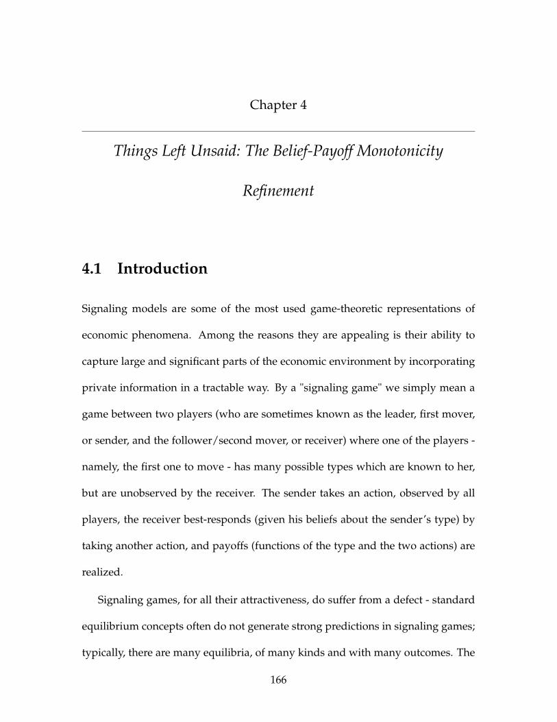
Chapter 4

Things Left Unsaid: The Belief-Payoff Monotonicity

Refinement

4.1 Introduction

Signaling models are some of the most used game-theoretic representations of

economic phenomena. Among the reasons they are appealing is their ability to

capture large and significant parts of the economic environment by incorporating

private information in a tractable way. By a "signaling game" we simply mean a

game between two players (who are sometimes known as the leader, first mover,

or sender, and the follower/second mover, or receiver) where one of the players -

namely, the first one to move - has many possible types which are known to her,

but are unobserved by the receiver. The sender takes an action, observed by all

players, the receiver best-responds (given his beliefs about the sender’s type) by

taking another action, and payoffs (functions of the type and the two actions) are

realized.

Signaling games, for all their attractiveness, do suffer from a defect - standard

equilibrium concepts often do not generate strong predictions in signaling games;

typically, there are many equilibria, of many kinds and with many outcomes. The

166

equilibria can be pooling (where all types take the same action), separating (where

all types take different actions), or mixed/hybrid (where the actions taken by dif-

ferent types do not follow a simple pattern), or more frequently, of all three kinds.

In other words, while signaling games are very useful representations, their pre-

dictive power may be limited. One way of moving past this problem is to resort

to so-called refinements of these equilibria to narrow down outcomes. A "refine-

ment" is simply a condition on the equilibrium conditions; if an equilibrium does

not satisfy such a condition it is said to fail the refinement. One then focuses only

on the equilibria that survive the refinement as a way of strengthening the predic-

tive content of the model.

The existing refinements aim to narrow down predictions by focusing on ac-

tions that are not taken on the equilibrium path of play. They rely on two princi-

ples; the first is often a version of the old adage "cui bono" - in other words, for

which types is a particular action beneficial, relative to a particular equilibrium?

The second principle seeks to adjust off path beliefs of the receiver about the type

of sender, following these off-path actions, so that they are consistent (in a sense

appropriate to the setting) with the types who benefit from those actions. For ex-

ample, if there is a single, unique type that benefits from a deviation, a widely used

refinement, the "intuitive criterion", requires the receiver to believe with probabil-

ity one that the deviation is coming from that type. There are a number of other

refinements of this type, many (though not all) of them based on the concept of

strategic stability proposed by Kohlberg and Mertens (1986). We review some of

167

the relevant refinements below1.

In this work we propose a new refinement, designed to work in a number of

settings. We further argue that it is not only a reasonable refinement, but is some-

times a necessary one. In addition, we posit that this new concept - which we call

belief-payoff monotonicity, or BPM for brevity - has a number of attractive prop-

erties. For example, it is strong in the sense that it can eliminate equilibria in some

games where others do not. Furthermore, it captures an appealing intuition - de-

viations must come from types that have the most to gain, if the receiver believes

the "message" that is implicitly sent by such a deviation2.

The motivation for the refinement we suggest is this: suppose that there is an

equilibrium and an associated (off-path) deviation so that multiple types benefit

for some beliefs of the receiver, but that at least one type benefits relatively more

than others. What should the receiver make of such a deviation, if observed? Cer-

tainly, any reasonable refinement would require the receiver to believe that the

deviation is coming from the set of types that benefit, but are there any additional

restrictions that may be desirable? Suppose for example, that while multiple types

all benefit, one type benefits greatly, while others benefit only slightly; it is reason-

able to stipulate that the receiver should believe that the deviation is coming from

the type for whom the gain is greatest. It is precisely this intuition that BPM is try-

ing to capture. This is also the reason for the nomenclature - the receiver’s beliefs

1We do not give definitions of these refinements, and instead point the reader to the originalarticles in the interests of keeping the present note short.

2Many other refinements attempt to capture a similar notion; we make these ideas precise andelucidate the ways in which out refinement is different in what follows.

168

conditional upon an off-equilibrium path action should be monotonic in the payoff

gain for each type of sender from choosing such an action. Thus, when multiple

types benefit from a deviation, but their gains from that deviation are different,

the receiver should assign higher probability to those types who benefit relatively

more. The reader may also note that this is a joint type-message-belief condition.

There are several ideas at play here. The key ones are the idea of forward

induction proposed by Kohlberg and Mertens (1986), and the notion of trembles

introduced (albeit in a slightly different setting - trembling-hand perfect equilib-

rium) by John Harsanyi. Forward induction attempts to interpret deviations in

some reasonable way - which is precisely what the BPM criterion is aiming to do

by explicitly prescribing what the beliefs should be. Harsanyi introduced the pos-

sibility that players may "tremble" and take deviated actions. Finally, Myerson

(1978) proposed that if players do tremble, they should tremble lexicographically

less often to actions that yield a lower payoff3. As discussed above, we adapt and

unite these ideas and take the stand that deviations (which we think of as trem-

bles) should be attributed to the types of sender than benefit the most from such a

deviation, provided the receiver holds exactly the beliefs that make this true.

There are a few questions that are behind much of the reasoning on refinements

and alternative equilibrium concepts - what do you make of a message that could

have been sent, but wasn’t (a "thing left unsaid"), what should you make of it, and

who would benefit as a result? The answer to these question is key in determining

3Quantal response equilibrium of McKelvey and Palfrey (1995) captures a similar idea in ex-periments - players make mistakes with probability that is proportional to the loss of a particularaction.

169

what sort of beliefs or equilibria are admissible; we explore a particular answer in

this note.

At this point the reader may justifiably wonder - why add a new refinement to

the already large bestiary of such beasts? The reason is that this refinement turns

out to work in a situation where others are unsatisfactory (see Kosenko (2018), the

first chapter of this dissertation). We view this refinement as not better or worse

than others - but we think that it may be helpful in some situations where others

remain silent. In addition, this refinement is quite "strong" qualitatively in that if

an equilibrium is ruled out by some other concept, it is probably4 ruled out by

BPM, so we view this refinement as one of last resort - if all others have failed,

BPM may be a reasonable option.

4.2 Environment

We are concerned with single period signaling games; the details of the environ-

ment and the notation are specified as follows. There is a finite set of types for the

sender: θ ∈ Θ, a finite set of states of the world ω ∈ Ω. Typically, the set of types

of the sender and the set of states of the world are identified, but could, in princi-

ple, be different; in this short chapter we do identify them for simplicity. Denote

by m ∈ M the message sent by the sender, and by a ∈ A the action taken by the

receiver. The utilities are uS(θ, m, a) for the sender and uR(θ, m, a) for the receiver.

Denote by σSθ and σR the respective strategies and let the final posterior beliefs of

4We formalize this below.

170

receiver be given by β.

Fix a PBE: e = σSθ , σR, β with associated equilibrium utilities u∗S(θ); suppose

for simplicity that A is a compact set and that β 7→ a(β) is one-to-one and onto;

in particular this means that we can drop the a argument from the sender’s utility.

We say that e fails the criterion if there exists a type θ ′, a message5 m ′, not sent in

equilibrium e with positive probability, and a belief of the receiver β(m ′) for which

the following is true:

Definition 18 (Belief-Payoff Monotonicity Refinement - BPM). Let e , σSθ , σR, β

be an equilibrium and let u∗(θ) be the equilibrium utility of type θ. Define, for a fixed m,

u(θi) , maxβ u(m, θi, β) and u(θi) , minβ u(m, θi, β). An equilibrium is said fail the

ε-BPM criterion if there is an experiment m, not chosen with positive probability in that

equilibrium and a type of sender, θi, such that:

i) Let β ∈ ∆(Ω) be an arbitrary belief of the receiver and suppose that δ(m, β, θi, e) ,

uS(m,θi,β)−u∗(θi)u(θi)−u(θi)

> 0, for that belief.

ii) Denote by K be the set of types for which (i) is true; if K is empty BPM is inoperative

so suppose that there is at least one type-message-belief triple for which i) holds. Let

θi be the type for which the difference is greatest. If there is another type θj in K, for

which δ(m, β, θi, e) > δ(m, β, θj, e) then let β(θj|m) < εβ(θi|m), for some positive

ε, with ε < 1|K| . If there is yet another type θk such that δ(m, β, θj, e) > δ(m, β, θk, e),

then let β(θk|m) < εβ(θj|m), and so on.

5We use the terminology of "messages" stemming from the cheap talk literature; this would justas well be some other "action".

171

iii) Beliefs are consistent: given the restrictions in (ii), the belief β is precisely the beliefs

that makes (i) true.

The reason for the normalization in part i) of the definition is to make the def-

inition stand up to affine transformations of the utility function (see also de Groot

Ruiz et al. (2011)). The third part of the definition is a consistency requirement; it

rules out situations such as the following. Suppose that the receiver believes that

the deviation is coming from a particular type (say, type i), but it is type j that

benefits more. Without the third requirement BPM would rule out such an equi-

librium, but clearly beliefs in that case are not internally consistent or reasonable.

Thus, one also has to check for internal consistency when applying BPM.

We say that an equilibrium fails the BPM criterion if it fails the ε-BPM criterion

for every admissible ε with ε going to zero. However, we view ε-BPM as the more

relevant refinement since it is more flexible6; we state the definition of BPM as a

limit since it is more intuitive and straightforward to apply.

This definition takes a clear, easily applicable stance on what beliefs should be

off-path. There are, of course, other stipulations one can make; we discuss these

possible differences now. One such stipulation, for example, is that the probability

assigned to a deviation should be proportional to the gain for a type (so that, for

example, if the gain for one type is twice the gain for another type, then the receiver

should believe that the deviation is coming from the first type with probability

two thirds, and from the second type with probability one third). This can be

6In particular, in the typical case there may be multiple types that benefit from a deviation; thereceiver may wish to assign some positive probability to the type that benefits less.

172

accommodated by choosing ε appropriately.

Another, perhaps more interesting issue is this: the definition given above fixes

a belief, and then considers a particular deviation. However, given a belief, there

may be multiple deviations for each type that can be beneficial - how should a

sender "tremble" among them, and what should the receiver believe? A reasonable

and strong7 definition may be the following. First, take an off-path belief for the

receiver, and compute the relative utilities from deviating to all actions, for each

type, given that belief. Then assume that each type will deviate to either sending

the message that is most beneficial, or that each type will tremble among the pos-

sible messages that are beneficial, and that lower-gain messages will be sent with

lower probability. And then apply ε-BPM for each message. This is arguably a

more encompassing refinement, and we note its potential usefulness. However, it

is also more complex and makes even more assumptions about behavior; we thus

focus on ε-BPM as a simpler and more easily applied definition.

Finally, we can draw one useful connection between BPM and proper equilib-

rium; both focus on similar trembles that are lexicographic in the (possible) gain.

However, proper equilibrium requires one to assign smaller probabilities to strate-

gies which are strictly dominated; whereas BPM requires the receiver to assign

smaller probabilities to types that benefit relatively less.

7And also related to reasoning behind proper equilibrium.

173

4.3 Relationship to Other Refinements

Performance relative to stability-based refinements

In this section we explore the relationship of BPM to refinements that are based

on the concept of strategic stability introduced by Kohlberg and Mertens (1986).

These refinements operate by restricting off-path beliefs, as does BPM.

The first observation is that BPM is prior-independent (unlike, for instance, di-

vine beliefs), so that it is more appropriate in this sense. Furthermore, it can accom-

modate (i.e. make meaningful selections in) a version of cheap talk games. Gen-

erally speaking, criteria such as D1 do not have any bite in cheap talk games since

they rely on messages that are unused in equilibrium, and in cheap talk games

there is always an outcome-equivalent equilibrium in which all messages are used

(for example, by randomizing over "unused" messages), and one is forced to re-

sort to other equilibrium concepts (such as neologism-proofness that is discussed

in the next section). BPM may, in fact, eliminate some cheap talk equilibria (as it

does in the first chapter of this dissertation; see Kosenko (2018)). Loosely speak-

ing, BPM can be stronger or weaker than other concepts in the sense that it can

do away with equilibria that are left untouched by other refinements, yet may also

fail to eliminate other equilibria that are eliminated by other refinements in some

cases.

We now turn to the question of examining the performance of BPM relative

to other common refinements. Instead of formulating specific examples, we give

simply a convenient representation of the relevant "moving parts" - the types of

174

sender, the beliefs of the receiver, and the utility changes as functions of those

beliefs. Well-chosen combinations of these moving parts will be sufficient to il-

lustrate the main ideas. We illustrate the workings of BPM in relation to three

commonly used (nested, and increasingly strict) refinements - the intuitive crite-

rion (IC), condition D1, and never a weak best response (NWBR) criterion. There

are many others in the same family (divinity, D2, iterated versions, etc) but they

are all nested in between these three, so by comparing BPM with them, we are also

implicitly illustrating its potential relative to all the others.

To fix ideas, suppose for simplicity that there are only two types of sender -

"red" and "blue", and fix some equilibrium as well as the corresponding equilib-

rium utilities. Suppose that the state of the world is the same as the type of the

sender. Take a particular deviation, and consider the utilities of the two types as

functions of the receiver’s beliefs. Generically, the utility from a deviation will

be different than the equilibrium utility; we thus plot the relative utility difference

from a deviation in the following figures.

In figure 4.1 we illustrate how the intuitive criterion and BPM operate. In the

typical case that is ruled out by IC, there are some beliefs of the receiver for which

one type but not the other, benefits. More precisely, in figure 4.1, equilibrium is

supported by beliefs β ∈ [0, β), which make this deviation unattractive to either

type. In that case, the equilibrium is said to fail IC - and it would also fail BPM,

since In other words, we can make the following

Observation 3. Suppose that an equilibrium fails the intuitive criterion. Then it also fails

175

β0

1

Uti

lity

diff

eren

ce

β

Figure 4.1: IC and BPM

the BPM criterion.

We omit the proof for brevity, but the intuition is clear from figure 4.1 - if there is

a unique type that benefits from a deviation foe some beliefs, both concepts require

one to believe that the deviation is coming from that type.

We now turn to the other frequently used refinement concept - condition D1

and show by example that BPM may or may not make the same equilibrium se-

lection. First we examine a case where they do, this is illustrated in figure 4.2.

D1 would eliminate this type-message pair (which clearly has to be supported by

some belief β ∈ (β†, 1]), since the set of beliefs for which the red type benefits

([0, β†)) is a strict superset of the set of beliefs for which the blue type benefits

([0, β)). Similarly, BPM would eliminate this type-message pair since there are be-

liefs for which the red type benefits relatively more.

176

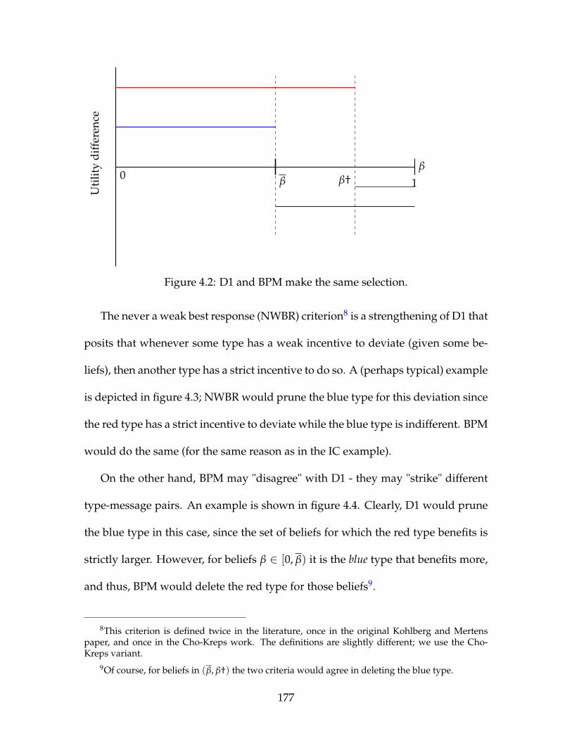
β0

1

Uti

lity

diff

eren

ce

β†β

Figure 4.2: D1 and BPM make the same selection.

The never a weak best response (NWBR) criterion8 is a strengthening of D1 that

posits that whenever some type has a weak incentive to deviate (given some be-

liefs), then another type has a strict incentive to do so. A (perhaps typical) example

is depicted in figure 4.3; NWBR would prune the blue type for this deviation since

the red type has a strict incentive to deviate while the blue type is indifferent. BPM

would do the same (for the same reason as in the IC example).

On the other hand, BPM may "disagree" with D1 - they may "strike" different

type-message pairs. An example is shown in figure 4.4. Clearly, D1 would prune

the blue type in this case, since the set of beliefs for which the red type benefits is

strictly larger. However, for beliefs β ∈ [0, β) it is the blue type that benefits more,

and thus, BPM would delete the red type for those beliefs9.

8This criterion is defined twice in the literature, once in the original Kohlberg and Mertenspaper, and once in the Cho-Kreps work. The definitions are slightly different; we use the Cho-Kreps variant.

9Of course, for beliefs in (β, β†) the two criteria would agree in deleting the blue type.

177

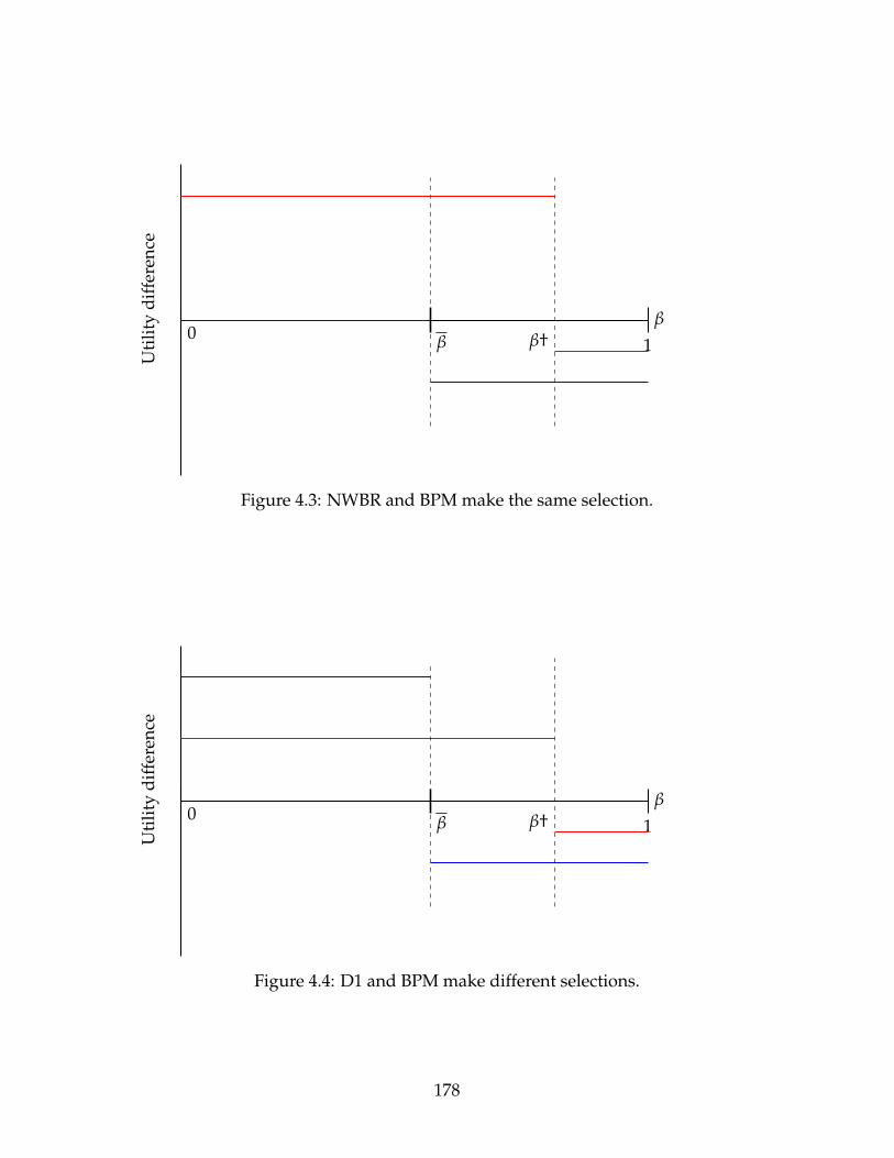
β0

1

Uti

lity

diff

eren

ce

β β†

Figure 4.3: NWBR and BPM make the same selection.

β0

1

Uti

lity

diff

eren

ce

β β†

Figure 4.4: D1 and BPM make different selections.

178

The two examples where D1 and BPM agree and disagree raise a reasonable

question - which of the two refinements is more convincing? The figures also sug-

gest that there is some interesting interplay between what D1 focuses on (the size

of the set of beliefs for which a type benefits) and the magnitude of the gain from

deviation, which is the focus of BPM. We illustrate this idea in figure 4.5 where

as before, D1 and BPM would "disagree". However, depending on how one inter-

prets trembles, either refinement may be more appealing. In this figure D1 would

delete the blue type since the set of beliefs for which the red type benefits is larger.

However, note that the red type benefits only a little (albeit for "more" beliefs),

while the blue type benefits quite a lot. In addition, the set of beliefs for which

the red type benefits is not that much smaller than the corresponding set for the

blue type. Given these two observations it is perfectly reasonable to delete the red

type for this deviation, which is what BPM would prescribe. In short, this exam-

ple shows that when BPM disagrees with other refinements, the question of which

one is "correct" is a subjective matter and depends on the particular case in point;

either can be plausible.

Finally, we give an example where D1 does not rule out any type-message

pairs, while BPM does. In figure 4.6 condition D1 is inoperative since the relative

sets are not nested. However, BPM would rule out both of these types.

We summarize the relation of BPM to stability-based refinement concepts in

figure 4.7. The nested concepts are depicted in black circles (with inclusion repre-

senting subsumption); the BPM refinement (represented by the red oval) may or

may not agree with the refinements that are strictly stronger than IC (and it may, in

179

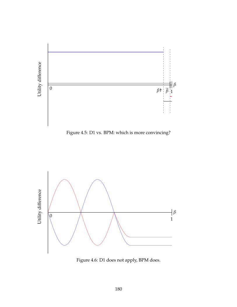
β0

1

Uti

lity

diff

eren

ce

ββ†

Figure 4.5: D1 vs. BPM: which is more convincing?

β0

1

Uti

lity

diff

eren

ce

Figure 4.6: D1 does not apply, BPM does.

180

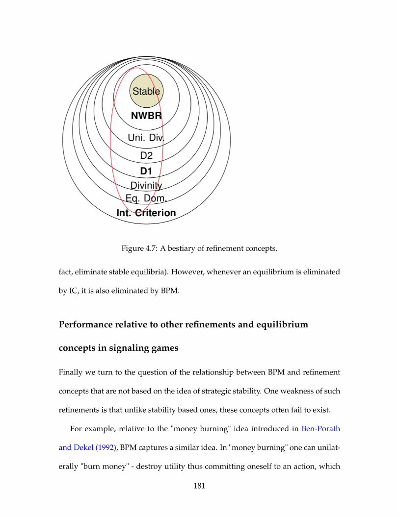
Figure 4.7: A bestiary of refinement concepts.

fact, eliminate stable equilibria). However, whenever an equilibrium is eliminated

by IC, it is also eliminated by BPM.

Performance relative to other refinements and equilibrium

concepts in signaling games

Finally we turn to the question of the relationship between BPM and refinement

concepts that are not based on the idea of strategic stability. One weakness of such

refinements is that unlike stability based ones, these concepts often fail to exist.

For example, relative to the "money burning" idea introduced in Ben-Porath

and Dekel (1992), BPM captures a similar idea. In "money burning" one can unilat-

erally "burn money" - destroy utility thus committing oneself to an action, which

181

forces the other player to respond appropriately. The point is that with this pos-

sibility some equilibria are eliminated even without actually burning money on

the equilibrium path - just the threat or possibility of this turns out to be enough.

The high type of sender can "afford to burn" relatively more than the low type.

In the absence of the option of burning actually payoffs (for example, in the stan-

dard examples from the Bayesian persuasion literature - an FDA drug trial and a

court trial - it is not clear how one would go about burning utility), ε-BPM offers a

simple reduced-form definition that captures much of the same logic with similar

results.

Similarly, relative to the concept of undefeated equilibria (Mailath et al. (1993)),

BPM operates in much the same way. There is an example however (see Kosenko

(2018)) where BPM rules out strictly more equilibria than undefeatedness. Like

undefeated equilibrium, BPM may rule out all equilibria - i.e. it may fail to exist10

However, Mailath et al. (1993) summarizes the undefeated equilibrium thus (p.

253):

Consider a proposed sequential equilibrium and a message for player

I that is not sent in equilibrium. Suppose there is an alternative se-

quential equilibrium in which some non-empty set of types of player I

choose the given message and that that set is precisely the set of types

who prefer the alternative equilibrium to the proposed equilibrium.

The test requires player II’s beliefs at that action in the original equi-

10An example, unfortunately, is the standard purely dissipative Spencian signaling.

182

librium to be consistent with this set. If beliefs are not consistent, we

say the second equilibrium defeats the proposed equilibrium.

Thus, Mailath et al. (1993) ask that there must be another equilibrium that de-

feats a putative equilibrium; BPM does not require that the alternative construction

be an equilibrium to eliminate a putative equilibrium.

Similarly, the perfect sequential equilibria of Grossman and Perry (1986) tries

to rationalize a deviation (once it occurs) by finding a set of types that benefit from

such a deviation. They do so by defining a metastrategy that specifies how this is

to be done; BPM would also eliminate equilibria that are not perfect sequential.

Note that both for perfect sequential and undefeated equilibria BPM would

eliminate at least as many equilibria as either of these concepts. This is because

if there exists an equilibrium that either defeats another, or a metastrategy that ra-

tionalizes a deviation, then surely there exist beliefs that satisfy the requirements

for BPM to eliminate an equilibrium - simply use the type-message-beliefs triple

in the defeating equilibrium.

Finally, BPM operates in a way that is analogous but not identical to the notion

of neologism-proof equilibria Farrell (1992). If an eq’m is neologism-proof, it will

survive BPM. However, BPM also takes a stand on how to "split" the probability

weighting among the types in a self-signaling set; neologism proofness does not

go that far. All three equilibrium concepts mentioned in this subsection may fail

to exist, just like BPM.

183


This note presents a definition a novel refinement of equilibria and briefly explores

its performance relative to other such concepts in the literature. The BPM criterion

has some of the flavor of stability-based refinement, being a restriction on off-path

beliefs, with the operative strength of other, newer equilibrium concepts. It seems

stronger than most other refinements but suffers from lack of existence. Whether

it will prove useful will be determined by its performance in future applications.

184

Bibliography

[1] Akerlof, George A, (1970), "The market for ’lemons’: Quality Uncertainty andthe Market Mechanism," Quarterly Journal of Economics, 84(3), pp. 488-500.

[2] Ales, Laurence and Pricila Maziero, (2012). "Adverse Selection and Non-exclusive Contracts," Working Paper, Carnegie Mellon University.

[3] Alonso, Ricardo and Odilon Camara, (2016). "Bayesian persuasion with hetero-geneous priors." Journal of Economic Theory, Volume 165, 2016, Pages 672-706,ISSN 0022-0531, http://dx.doi.org/10.1016/j.jet.2016.07.006.

[4] Alonso, Ricardo and Odilon Camara, (2016a). "On the value of persua-sion by experts". Working paper. Available at http://www-bcf.usc.edu/ oca-mara/PersuasionExperts.pdf

[5] Alonso, Ricardo and Odilon Camara, (2016b) "Persuading Voters". Forthcom-ing, American Economic Review.

[6] Ambrus, A., Azevedo, E. M. and Kamada, Y, (2013), Hierarchical cheap talk.Theoretical Economics, 8: 233-261. doi:10.3982/TE1038

[7] Arieli, Itai and Yakov Babichenko, (2016). "Private Bayesian Persuasion". Work-ing paper.

[8] Arnott, Richard J. and Joseph E. Stiglitz (1987, 2013), "Equilibrium in competi-tive insurance markets with moral hazard." in The Selected Works of Joseph E.Stiglitz, Volume II: Information and Economic Analysis: Applications to Cap-ital, Labor, and Product Markets, Oxford: Oxford University Press, 2013, pp.660- 689. Edited version of Princeton University Discussion Paper 4, 1987

[9] Arnott, Richard J. and Joseph E. Stiglitz (1991a, 2013), "Price Equilibrium, Effi-ciency, and Decentralizability in Insurance Markets," in The Selected Works ofJoseph E. Stiglitz, Volume II: Information and Economic Analysis: Applicationsto Capital, Labor, and Product Markets, Oxford: Oxford University Press, 2013,pp. 632-659. Edited version of NBER Working Paper 3642, 1991.

185

[10] Arnott, Richard J. and Joseph E. Stiglitz, (1991b). "Moral Hazard and Nonmar-ket Institutions: Dysfunctional Crowding Out or Peer Monitoring?" AmericanEconomic Review, 81(1), pp. 179-90.

[11] Arrow, Kenneth J, (1965). Aspects of the Theory of Risk-Bearing, Yrjo JahnssonLectures, Helsinki, Finland: Yrjo Jahnssonin Saatio.

[12] Attar, Andrea, Thomas Mariotti, and Francois Salanie, (2011), "NonexclusiveCompetition in the Market for Lemons," Econometrica, 79(6), 1869-1918.

[13] Attar, Andrea, Thomas Mariotti, and Francois Salanie, (2014), "NonexclusiveCompetition under Adverse Selection," Theoretical Economics, 9(1), pp. 1-40.

[14] Attar, Andrea, Thomas Mariotti, and Francois Salanie, (2016), "Multiple Con-tracting in Insurance Markets," Working Paper, TSE-532.

[15] Aumann, Robert and Michael Maschler, (1995). Repeated Games with IncompleteInformation. The MIT Press.

[16] Banks, Jeffrey S. and Sobel, Joel, (1987). "Equilibrium Selection in SignalingGames," Econometrica, Econometric Society, vol. 55(3), pages 647-61, May.

[17] Ben-Porath, Elchanan and Eddie Dekel, (1992). "Signaling future actions andthe potential for sacrifice", Journal of Economic Theory, Volume 57, Issue 1,Pages 36-51.

[18] Blackwell, David, (1951). "Comparison of Experiments." Proceedings of theSecond Berkeley Symposium on Mathematical Statistics and Probability, 93–102,University of California Press, Berkeley, Calif.

[19] Blackwell, David, (1953). "Equivalent Comparisons of Experiments." Ann.Math. Statist. 24, no. 2, 265–272.

[20] Blume, Andreas, (2012). "A class of strategy-correlated equilibria in sender-receiver games." Games and Economic Behavior, vol. 75. no. 2, pp. 510-517.

[21] Blume, Andreas, Oliver J. Board and Kohei Kawamura, (2007). "Noisy Talk."Theoretical Economics, vol. 2, no. 4. pp.395-440.

[22] Chen, Y., Kartik, N. and Sobel, J., (2008). "Selecting Cheap-Talk Equilibria."Econometrica, vol. 76, pp. 117-136.

186

[23] Cho, In-Koo, and David M. Kreps, (1987). "Signaling Games and Stable Equi-libria." The Quarterly Journal of Economics, vol. 102, no. 2, pp. 179-221.

[24] Cho, In-Koo and Joel Sobel, (1990). "Strategic Stability and Uniqueness in Sig-naling Games". Journal of Economic Theory, 50, 381-413.

[25] Coval, Joshua D. and Jurek, Jakub W. and Stafford, Erik, The Economics ofStructured Finance (October 20, 2008). Harvard Business School Finance Work-ing Paper No. 09-060. Available at SSRN: https://ssrn.com/abstract=1287363 orhttp://dx.doi.org/10.2139/ssrn.1287363

[26] Crawford, Vincent P., and Joel Sobel, (1982). "Strategic Information Transmis-sion." Econometrica, vol. 50, no. 6, pp. 1431-1451.

[27] Dasgupta, Partha and Eric Maskin (1986), "The Existence of Equilibrium inDiscontinuous Games: I," Review of Economic Studies, 53(1), pp. 1-26.

[28] Farinha Luz, V, (2017). "Characterization and uniqueness of equilibrium incompetitive insurance." Theoretical Economics, 12: 1349-1391.

[29] de Groot Ruiz, Andrian, Theo Offerman and Sander Onderstal, (2013). "Equi-librium Selection in Cheap Talk Games: ACDC Rocks When Other Criteria Re-main Silent." Working paper.

[30] de Groot Ruiz, Andrian, Theo Offerman and Sander Onderstal, (2013). "Equi-librium Selection in Cheap Talk Games: ACDC Rocks When Other Criteria Re-main Silent." Working paper.

[31] Degan, Arianna and Li, Ming, (2015). "Persuasive Signalling" Work-ing paper, available at SSRN: http://ssrn.com/abstract=1595511 orhttp://dx.doi.org/10.2139/ssrn.1595511

[32] Farrell, Joseph, (1993). "Meaning and Credibility in Cheap-Talk Games",Games and Economic Behavior, Volume 5, Issue 4, Pages 514-531.

[33] Geanakoplos, John, (1989). "Game Theory without Partitions, with Applica-tions

[34] Gentzkow, Matthew and Emir Kamenica, (2017a). "Competition in Persua-sion." Review of Economic Studies, vol. 84, no. 4, pp. 300-322.

187

[35] Gentzkow, Matthew and Emir Kamenica, (2017b). "Bayesian persuasion withmultiple senders and rich signal spaces." Games and Economic Behavior, Vol-ume 104, Pages 411-429, https://doi.org/10.1016/j.geb.2017.05.004.

[36] Gill, David and Daniel Sgroi, (2012). "The optimal choice of pre-launch re-viewer". Journal of Economic Theory, 147(3), 1247/1260

[37] Greenwald, Bruce and J. E. Stiglitz, (1986), "Externalities in Economies withImperfect Information and Incomplete Markets," The Quarterly Journal of Eco-nomics, Volume 101, Issue 2, 1 May 1986, Pages 229-264.

[38] Grossman, Sanford, (1981). "The Informational Role of Warranties and PrivateDisclosure about Product Quality", Journal of Law and Economics, 24, issue 3,p. 461-83.

[39] Grossman, Sanford J. and Moty Perry, (1986). "Perfect Sequential Equilib-rium", Journal of Economic Theory, Volume 39, Issue 1, Pages 97-119.

[40] Hedlund, Jonas, (2017). "Bayesian persuasion by a privately informedsender". Journal of Economic Theory, Volume 167, January 2017, Pages 229-268,ISSN 0022-0531, https://doi.org/10.1016/j.jet.2016.11.003.

[41] Hellwig, Martin F, (1987), "Some Recent Developments in the Theory of Com-petition in Markets with Adverse Selection," European Economic Review, 31(1-2), pp. 309-325.

[42] Hellwig, Martin F, (1988), "A note on the specification of interfirm communi-cation in insurance markets with adverse selection," Journal of Economic The-ory, 46(1), pp. 154-163.

[43] Jaynes, Gerald D, (1978), "Equilibria in monopolistically competitive insur-ance markets," Journal of Economic Theory, 19(2), pp. 394-422.

[44] Jaynes, Gerald D, (2011), "Equilibrium and Strategic Communication in theAdverse Selection Insurance Model," Working Paper, Yale University.

[45] Kamenica, Emir, and Matthew Gentzkow, (2011). "Bayesian Persuasion."American Economic Review, 101(6): 2590-2615.

[46] Kohlberg, Elon, and Jean-Francois Mertens, (1986). "On the Strategic Stabilityof Equilibria." Econometrica, vol. 54, no. 5, pp. 1003-1037.

188

[47] Kosenko, Andrew, (2017). "Bayesian Persuasion with Private Information."Working paper. Available at: http://www.columbia.edu/ ak2912/

[48] Kreps, David M and Wilson, Robert, (1982). "Sequential Equilibria," Econo-metrica, Econometric Society, vol. 50(4), pages 863-94, July.

[49] Lehmann, E. L, (1988). "Comparing Location Experiments." The Annals ofStatistics, vol. 16, no. 2, pp. 521-533.

[50] Li, Fei and Norman, Peter. "Sequential Persuasion" Working Paper,(May 12, 2017). Available at SSRN: https://ssrn.com/abstract=2952606 orhttp://dx.doi.org/10.2139/ssrn.2952606

[51] Mailath, George J., Masahiro Okuno-Fujiwara, Andrew Postlewaite, (1993)"Belief-Based Refinements in Signalling Games", Journal of Economic Theory,Volume 60, Issue 2, Pages 241-276.

[52] Mailath, George J., et al. (1993). "Extensive Form Reasoning in Normal FormGames." Econometrica, vol. 61, no. 2, pp. 273-302.

[53] Matthews, Steven A., Masahiro Okuno-Fujiwara, Andrew Postlewaite. "Re-fining cheap-talk equilibria", Journal of Economic Theory, Volume 55, Issue 2,1991, Pages 247-273.

[54] McKelvey, R. D., and Palfrey, T. R, (1998). "Quantal Response Equilibrium forExtensive Form Games." Experimental Economics, 1, pp 9-41.

[55] McKelvey, Richard D. and Thomas R. Palfrey, (1995). "Quan-tal Response Equilibria for Normal Form Games." Games and Eco-nomic Behavior, Volume 10, Issue 1, Pages 6-38, ISSN 0899-8256,http://dx.doi.org/10.1006/game.1995.1023.

[56] Milgrom, Paul, (1981). "Good News and Bad News: Representation Theoremsand Applications", Bell Journal of Economics, 12, issue 2, p. 380-391.

[57] Milgrom, Paul and Shannon, Chris, (1994). "Monotone Comparative Statics,"Econometrica, Econometric Society, vol. 62(1), pages 157-80, January.

[58] Myerson, R, (1978). "Refinements of the Nash Equilibrium Concept." Interna-tional Journal of Game Theory, vol. 7, pp. 73-80.

189

[59] Myerson, Roger B, (1983). "Mechanism Design by an Informed Principal."Econometrica, vol. 51, no. 6, pp. 1767-1797.

[60] Netzer, N. and Scheuer, F, (2014), "A Game Theoretic Foundation of Com-petetive Equilibria with Adverse Selection". International Economic Review, 55:399-422.

[61] Osborne, Martin J. and Ariel Rubinstein, (1994). A Course in Game Theory. MITPress, Cambridge, MA.

[62] Perez-Richet, Eduardo, (2014). "Interim Bayesian Persuasion: First Steps".American Economic Review: Papers & Proceedings, 104, 5.

[63] Persico, Nicola, (2000). "Information Acquisition in Auctions". Econometrica,vol. 68(1), pp. 135-148.

[64] Pollrich, Martin, (2017). "Mediated audits." The RAND Journal of Economics,48: 44-68. doi:10.1111/1756-2171.12167

[65] Rahman, David and Ichiro Obara, (2010). "Mediated Partnerships." Econo-metrica, 78: 285-308. doi:10.3982/ECTA6131

[66] Rayo, L., and Segal, I, (2010). "Optimal Information Disclosure". Journal ofPolitical Economy, 118(5), 949-987.

[67] Riley, John, (1979). "Informational Equilibrium," Econometrica, 47(2), pp. 331-359.

[68] Rothschild, Michael and Joseph E. Stiglitz, (1976). "Equilibrium in competi-tive insurance markets: An essay on the economics of imperfect information,"Quarterly Journal of Economics, 90, pp. 629-649.

[69] Rothschild, Michael and Joseph E. Stiglitz, (1997). "Competition and Insur-ance Twenty Years Later" Geneva Papers on Risk and Insurance Theory, 22(2),pp. 73-79.

[70] Sah, Raaj Kumar, and Joseph E. Stiglitz, (1986). "The Architecture of EconomicSystems: Hierarchies and Polyarchies." The American Economic Review, vol.76, no. 4, pp. 716-727.

190

[71] Samuelson, Larry, (2004). "Modeling Knowledge in Economic Analysis," Jour-nal of Economic Literature, vol. 42, pp. 367-403.

[72] Selten, R, (1975) "Reexamination of the perfectness concept for equilib-rium points in extensive games". International Journal of Game Theory 4: 25.doi:10.1007/BF01766400

[73] Spence, Michael A., (1973). "Job Market Signaling." The Quarterly Journal ofEconomics, vol. 87, no. 3, pp. 355-374.

[74] Stiglitz, Joseph E., (1977). "Monopoly, Non-Linear Pricing and Imperfect In-formation: The Insurance Market," Review of Economic Studies, 44(3), pp. 407-430.

[75] Stiglitz, Joseph E., (2009), "Introduction to Part IIB," in Selected Works ofJoseph E. Stiglitz, Volume I: Information and Economic Analysis, Oxford: Ox-ford University Press, 2009, pp. 129-140.

[76] Stiglitz, Joseph and J. Yun (2016), "Equilibrium in a Competitive InsuranceMarket with Non-exclusivity Under Adverse Selection," mimeo.

[77] Taneva, Ina, (2016). "Information Design." Working paper, available athttps://sites.google.com/site/itaneva13/research

[78] Wilson, C, (1977). "A model of insurance markets with incomplete informa-tion," Journal of Economic Theory, 16(2), pp. 167-207. Econometric Society, vol.55(3), pages 647-61, May.

191

essays in economic theory: strategic communication and

Documents