Essays on Microeconomic Theory

Adriano Basso

A DissertationPresented to the Facultyof Princeton University

in Candidacy for the Degreeof Doctor of Philosophy

Recommended for Acceptanceby the Department ofEconomicsAdviser: Wolfgang Pesendorfer

June 2012

c© Copyright by Adriano Basso, 2012.All rights reserved.

Abstract

This collection of essays investigates issues related to information acquisition in thepresence of permanent ambiguity, perception errors or computational constraints.After a brief introduction, Chapter 1 introduces a decision maker who faces a sequenceof non-identical experiments with a finite numbers of possible outcomes. The lawgenerating the observations changes from period to period and the decision makerdoes not know anything about how the laws evolve. She has probabilistic beliefsover sets of possible laws and makes inferences on the true set of laws. I considerupdating mechanisms characterized by consequentialism and such that updating canonly depend on current beliefs and the current observation. To stay as close aspossible to the standard Bayesian framework, I assume that the relative frequenciesof observations converges to some limit frequency and that this limit frequency iscompatible with only one of the possible sets of laws. I then show that, when thenumber of possible outcomes is larger than three, the individual may never learn whatthe true set of laws is.

In Chapters 2 and 3 I consider a decision maker receiving signals. The signalsspecify a subset of the set S of states of the world in which the true state in included.However, the decision maker does not observe the signals correctly: each signal isperceived as a possibly different subset of S according to a function v mapping truesignals into perceived ones. Chapter 2 introduces the concepts of underconfidence andoverconfidence for this setting and analyzes the consequences of different behavioralsources of misperception on the set of fixed points of the mapping function v and onthe relation between each true signal A and the corresponding perceived signal v(A).In Chapter 3 I add an ex-ante stage to the model. The decision maker is aware of herability to manage a limited number of different signals, smaller than the total numberof signals that she may receive. She therefore chooses an optimal function v mappingreceived signals into perceived ones, subject to the constraint on the number of thelatter. The chapter studies the properties of this optimal mapping.

iii

Acknowledgements

The essays in this dissertation would have never been written without the constantguidance and generous help of my adviser, Professor Wolfgang Pesendorfer. I alsowant to thank Professor Faruk R. Gul and Professor Stephen E. Morris for their usefulcomments.

Many people gave me their support during my years of Graduate School, allowingme to overcome the most difficult periods of this intense experience. My family, firstof all, and then the friends I had the good fortune to meet in Princeton: Ling LingAng, Francesco Bianchi, Elisa Giaccaglia, Francesca Leoni and Alfonso Sorrentino.

Finally, a special thanks to Jayanti Chamling Rai, who has brightened my daysduring the last year.

iv

To Jayanti, whom I love without ambiguity

v

Contents

Abstract . . . . . . . . . . . . . . . . . . . . . . . . . . . . . . . . . . . . . iiiAcknowledgements . . . . . . . . . . . . . . . . . . . . . . . . . . . . . . . iv

Introduction 1

1 Recursive Mechanisms for Updating Beliefs over Sets of Laws 31.1 Introduction . . . . . . . . . . . . . . . . . . . . . . . . . . . . . . . . 3

1.1.1 Preliminary Example . . . . . . . . . . . . . . . . . . . . . . . 31.1.2 Existing Literature and Plan of the chapter . . . . . . . . . . 6

1.2 Non-identical Experiments and Beliefs . . . . . . . . . . . . . . . . . 81.2.1 The Model . . . . . . . . . . . . . . . . . . . . . . . . . . . . . 81.2.2 Differences with Respect to the Epstein-Seo Model . . . . . . 10

1.3 Recursive Updating Rule . . . . . . . . . . . . . . . . . . . . . . . . . 111.4 Updating Rules and Long Run Beliefs . . . . . . . . . . . . . . . . . . 131.5 Conclusions . . . . . . . . . . . . . . . . . . . . . . . . . . . . . . . . 15

2 Updating and Misperception of Signals 172.1 Introduction . . . . . . . . . . . . . . . . . . . . . . . . . . . . . . . . 172.2 Framework . . . . . . . . . . . . . . . . . . . . . . . . . . . . . . . . . 192.3 Indistinguishable Signals . . . . . . . . . . . . . . . . . . . . . . . . . 212.4 Dominated States . . . . . . . . . . . . . . . . . . . . . . . . . . . . . 222.5 Response to Information Increases . . . . . . . . . . . . . . . . . . . . 242.6 Conclusions . . . . . . . . . . . . . . . . . . . . . . . . . . . . . . . . 26

3 Optimal Underconfidence and Overconfidence 283.1 Introduction . . . . . . . . . . . . . . . . . . . . . . . . . . . . . . . . 283.2 The Model . . . . . . . . . . . . . . . . . . . . . . . . . . . . . . . . . 303.3 General Results and Conjectures . . . . . . . . . . . . . . . . . . . . 32

3.3.1 Properties of optimal sets V . . . . . . . . . . . . . . . . . . . 323.3.2 Properties of optimal functions v . . . . . . . . . . . . . . . . 333.3.3 Further observations . . . . . . . . . . . . . . . . . . . . . . . 34

3.4 The Case of Two States . . . . . . . . . . . . . . . . . . . . . . . . . 373.5 The Case of Three States . . . . . . . . . . . . . . . . . . . . . . . . . 383.6 Conclusions . . . . . . . . . . . . . . . . . . . . . . . . . . . . . . . . 40

vi

A Proofs for Chapter 1 41A.1 Proof of Theorem 1.4.1 . . . . . . . . . . . . . . . . . . . . . . . . . . 41A.2 Proof of Theorem 1.4.2 . . . . . . . . . . . . . . . . . . . . . . . . . . 45A.3 Proof of Lemma 1.4.1 . . . . . . . . . . . . . . . . . . . . . . . . . . . 51

B Proofs for Chapter 2 52B.1 Proof of Proposition 2.3.1 . . . . . . . . . . . . . . . . . . . . . . . . 52B.2 Proof of Proposition 2.4.1 . . . . . . . . . . . . . . . . . . . . . . . . 53B.3 Proof of Corollary 2.4.1 . . . . . . . . . . . . . . . . . . . . . . . . . . 55B.4 Proof of Proposition 2.5.1 . . . . . . . . . . . . . . . . . . . . . . . . 56B.5 Proof of Proposition 2.5.2 . . . . . . . . . . . . . . . . . . . . . . . . 56

C Matlab Code and Numerical Examples for Chapter 3 57C.1 Matlab Code . . . . . . . . . . . . . . . . . . . . . . . . . . . . . . . 57C.2 Optimal Sets V for the Case of Three States . . . . . . . . . . . . . . 59

Bibliography 61

vii

Introduction

The chapters of this dissertations analyze the problem of beliefs updating from threedifferent points of view, exploring issues related to information acquisition in the pres-ence of permanent ambiguity, perception errors or computational constraints. In thesecontexts, the traditional Bayesian updating algorithm is either inapplicable (as in thecase of ambiguity) or it produces unusual results (as in the case of misperceptions).

The model presented in Chapter 1 describe a situation of permanent ambiguity.A decision maker who faces a sequence of non-identical experiments with a finitenumbers of possible outcomes. The law generating the observations changes fromperiod to period and the decision maker does not know anything about how thelaws evolve. Moreover, she thinks that no information can be obtained on that.She therefore thinks in terms of sets of probability distributions, or laws: from aset of possible laws, one is selected in each period to generate the observation. Thedecision maker has probabilistic beliefs over sets of laws. The absence of a probabilisticbelief over laws (in contrast to one over sets of laws) gives rise to ambiguity. Theimpossibility of acquiring information on how the laws evolve makes this ambiguitypermanent.

As in any model of ambiguity, it is not obvious what a reasonable mechanismfor updating beliefs should look like. In this work, I consider updating mechanismscharacterized by consequentialism and by a strong restriction of the amount of infor-mation that the decision maker can use: updating can only depend on current beliefsand the current observation. The purpose of Chapter 1 is to verify whether, as in amodel with no ambiguity, this limited information is sufficient to asymptotically learnthe true set of laws. To stay as close as possible to the standard Bayesian framework,I assume that the relative frequencies of observations converges to some limit fre-quency and that this limit frequency is compatible with only one of the possible setsof laws. The main result is that the individual may never learn what the true set oflaws is. Interestingly enough, the impossibility result emerges only when the numberof possible outcomes is larger than three. For a smaller number of outcomes, learningis always possible.

In the last two chapter, the decision maker is an expected utility maximizer andupdates her beliefs through Bayes rule. Her behavior is, however, non-standard, be-cause perception errors or the impossibility to handle too much information influencethe way in which updating takes place.

In Chapters 2 and 3 the decision maker, before choosing an act, receives a signal.The signal specifies a subset of the set S of states of the world in which the true

1

state in included. After observing the signal, the decision maker updates her prioraccording to Bayes rule and then chooses an act that maximizes her utility. However,she does not observe the signals correctly: each signal is perceived as a possiblydifferent subset of S, according to a function v mapping true signals into perceivedones.

Chapter 2 analyzes the consequences of different behavioral sources of misper-ception on the characteristics of the mapping function v. In particular, I study theproperties of set of fixed points of the mapping function v and the relation betweeneach true signal A and the corresponding perceived signal v(A). The chapter alsointroduces the concepts of underconfidence and overconfidence for this setting as arelation between received and perceived signals.

Chapter 3 continues the analysis of the model, adding an ex-ante stage. Thedecision maker is aware of her ability to manage just a limited number of differentsignals, smaller than the total number of signals that she may receive. Therefore, exante, she chooses an optimal function v mapping received signals into perceived ones,subject to the constraint on the number of the latter. Instead of perception errors, themodel can be seen as describing a constraint in the amount of information that thedecision maker can handle. The difference between received and perceived signals isnow endogenous. The chapter studies the properties of the optimal mapping functionv.

2

Chapter 1

Recursive Mechanisms forUpdating Beliefs over Sets of Laws

1.1 Introduction

1.1.1 Preliminary Example

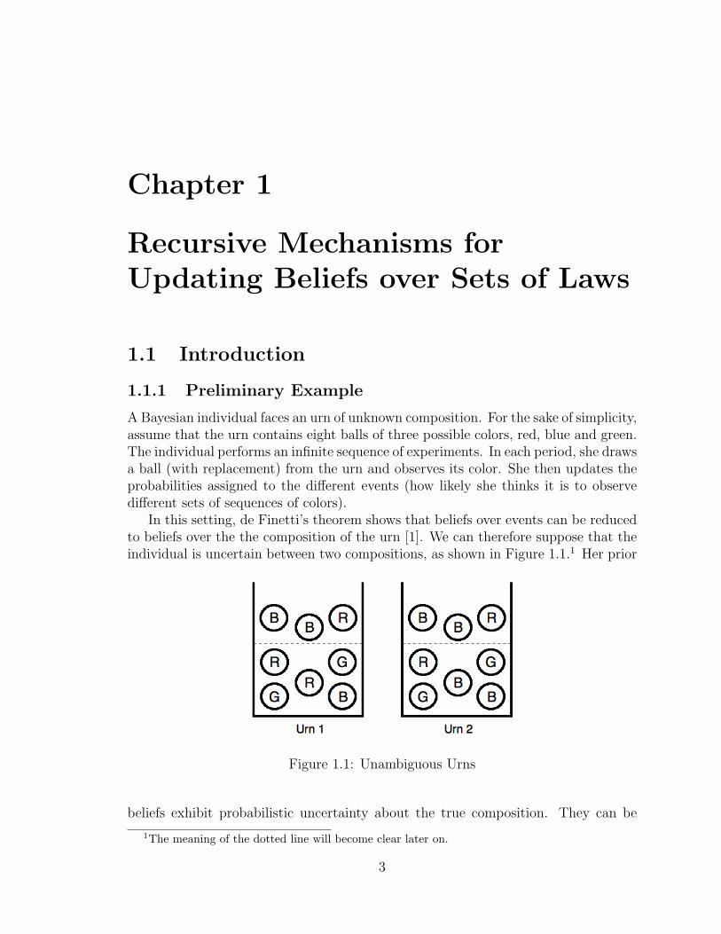
A Bayesian individual faces an urn of unknown composition. For the sake of simplicity,assume that the urn contains eight balls of three possible colors, red, blue and green.The individual performs an infinite sequence of experiments. In each period, she drawsa ball (with replacement) from the urn and observes its color. She then updates theprobabilities assigned to the different events (how likely she thinks it is to observedifferent sets of sequences of colors).

In this setting, de Finetti’s theorem shows that beliefs over events can be reducedto beliefs over the the composition of the urn [1]. We can therefore suppose that theindividual is uncertain between two compositions, as shown in Figure 1.1.1 Her prior

Figure 1.1: Unambiguous Urns

beliefs exhibit probabilistic uncertainty about the true composition. They can be

1The meaning of the dotted line will become clear later on.

3

represented with a probability distribution µ0 over the two possible compositions. Ineach period, after observing the color of the ball, the individual updates her currentbeliefs in a Bayesian way. Once beliefs have been updated, she forgets both theobservation and her past beliefs.

This is a very standard model. For future reference, it is useful to emphasizetwo important features of it. On the one hand, the relative frequencies of the colorsobserved converge in the long run to the true composition of the urn. On the otherhand, the individual’s beliefs µt converge to a degenerate distribution that assignsprobability 1 to the true composition. Notice that this long-run identification isreached even if the individual makes use of a very limited amount of information. Inparticular, she is not aware of the values of the relative frequencies.

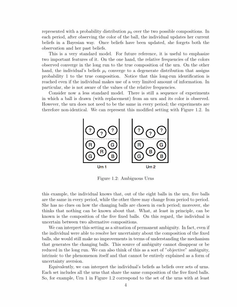
Consider now a less standard model. There is still a sequence of experimentsin which a ball is drawn (with replacement) from an urn and its color is observed.However, the urn does not need to be the same in every period; the experiments aretherefore non-identical. We can represent this modified setting with Figure 1.2. In

Figure 1.2: Ambiguous Urns

this example, the individual knows that, out of the eight balls in the urn, five ballsare the same in every period, while the other three may change from period to period.She has no clues on how the changing balls are chosen in each period; moreover, shethinks that nothing can be known about that. What, at least in principle, can beknown is the composition of the five fixed balls. On this regard, the individual isuncertain between two alternative compositions.

We can interpret this setting as a situation of permanent ambiguity. In fact, even ifthe individual were able to resolve her uncertainty about the composition of the fixedballs, she would still make no improvements in terms of understanding the mechanismthat generates the changing balls. This source of ambiguity cannot disappear or bereduced in the long run. We can also think of this as a sort of ”objective” ambiguity,intrinsic to the phenomenon itself and that cannot be entirely explained as a form ofuncertainty aversion.

Equivalently, we can interpret the individual’s beliefs as beliefs over sets of urns.Each set includes all the urns that share the same composition of the five fixed balls.So, for example, Urn 1 in Figure 1.2 correspond to the set of the urns with at least

4

one red, two blue and two green balls. The convex hulls of the sets correspondingto the urns in Figure 1.2 are shown in Figure 1.3.2 The darker triangle corresponds

Figure 1.3: Sets of Urns

to Urn 1, the other to Urn 2. Notice that the sets are triangle; more precisely, theyare similar to the simplex and differ from each other by a translation. The area ofthe triangles depends on the ratio between changing and fixed balls. As the exampleshows, the sets can intersect. We can think of these sets as ”sets of laws”, wherea law is a probability distribution that, in a given period, assigns probabilities tothe different colors that can be observed. A set of laws, therefore, can be used as adescription of a sequence of non-identical experiments.

In order to remain as close as possible to the standard Bayesian model, I willassume that the individual has probabilistic uncertainty over possible sets of laws;that is, over the two possible compositions of the fixed balls. In each period, theindividual draws a ball (with replacement) and observes its color. She then updatesher beliefs and, after that, forgets the observation and her past beliefs. Therefore, theinformation that the individual can use for updating is the same as in the standardmodel. The class of rules for updating the probabilistic beliefs over sets of lawsmaking use of this limited information will be denoted in this chapter as the classof ”recursive updating rules”. The term ”recursive” underlines the fact that theupdating algorithm is the same in every period: it is a function of current beliefs andof the current observation.3

To make things even more similar, I make an additional assumption on the se-quence of observations. Since nothing is known about the mechanism that selects thechanging balls, there is no guarantee of convergence of the relative frequencies of the

2In the rest of the chapter, I will consider convex sets. So, in this discrete example, it makessense to look at the convex hulls.

3The standard Bayesian rule is an example of recursive updating rule. However, even in a non-ambiguous setting, one can think of many more recursive rules.

5

colors observed. By analogy with the Bayesian model, I assume that such a conver-gence takes place. Moreover, I require that this limit frequency is compatible withone and only one set of urns. That is, I assume that the limit frequency is a pointbelonging to only one of the convex hulls of the two possible sets, and not to theirintersection. With this assumption I exclude the cases of ”undecidability”; in fact, itis clear that, if the individual were able to keep track of the relative frequencies, inthe long run she would identify the true set of urns.

Given these analogies with the Bayesian model, one may wonder whether similarlimit beliefs can be obtained. Since in the non-ambiguous case the beliefs of a Bayesianindividual converge to a degenerate distribution assigning probability one to the trueurn, can a similar result hold in a model of permanent ambiguity? That is, is itpossible for the individual, in the long run, to identify the true composition of thefixed balls using some recursive updating rule? This is the question that I addressin the present chapter. The model I use will be, of course, more general than thispreliminary example. In particular, I will allow for an arbitrary finite number ofoutcomes (or colors). Notice, however, that the generalizations would not underminethe convergence result in the non-ambiguous case.

I will prove that, under mild regularity conditions, convergence to the true setof laws is not generally possible. In particular, problems arise when the number ofoutcomes (colors) is higher than three. The main result of this chapter is thereforean impossibility theorem. For up to three outcomes, on the other hand, we do havea result analogous to the usual Bayesian one.

1.1.2 Existing Literature and Plan of the chapter

The idea that a decision maker could interpret a sequence of experiments as beingnon-identical was first considered by Epstein and Schneider [3], who define the notionof indistinguishability as opposed to independence. Sequences of non-identical exper-iments were then explicitly introduced in the economic literature by Epstein and Seo[4]. Notice, however, that similar ideas had been developed in a statistical context;see for example Fierens and Fine [6].

Epstein and Seo provide a behavioral characterization of a utility function thatwill be used in the present chapter. I will not go over the axioms; here I just want tospend a few words on the interpretation of the function. Let S be the set of outcomesof each experiment; that is, the set of possible colors of a ball. The state space is thengiven by Ω = S∞. Let Σ be the product σ-algebra on Ω. An act f is a Σ-measurablefunction from Ω to [0, 1]. The decision maker’s preference relation can be representedby a utility function of the form

U(f) =

∫ (minL∞

∫fdP

)dµ(L),

where

6

• L is a closed and convex set of probability distributions over outcomes that cancharacterize an experiment; it correspond to the (convex hull of) a set of urnsas described in the example above; in my terminology, it is a set of laws;

• P is a probability measure on (Ω,Σ); it is a distribution over sequences ofoutcomes (sequences of colors, in the example above), constructed taking onelaw in L for each period and considering the experiments as independent;

• µ is a probability distribution over sets of laws; it describes the decision maker’sprobabilistic uncertainty over sets (that is, in my example, over compositionsof the fixed balls in the urn).

With a change of notation, it is possible to show that this representation is aspecial case of the multiple-prior utility function axiomatized by Gilboa and Schmei-dler [9]. The interested reader can look at [4]. Notice, however, that the source ofambiguity in this model is different from that implied in the traditional interpretationof the Ellsberg paradox. Usually, the decision maker is seen as unable to express heruncertainty on the value of the relevant parameter in terms of a probability distri-bution. Here, on the other hand, the relevant parameter is the set of laws L, andthe decision maker does have probabilistic uncertainty over its value. The ambiguityemerges from the relation between the parameter and the outcomes. The differencebecomes crucial when we think about belief updating. In this context, the standardgeneralized Bayesian rule, as axiomatized in Pires [13], that consists in the Bayesianupdating of each prior, does not make sense. The reason is that there is not a naturallikelihood function to use. Updating becomes a more subtle problem. The presentchapter addresses some of the issues emerging when we try to model the process ofupdating beliefs over sets of laws.

The problem of belief updating in the case of non-identical experiments was firststudied within a statistical framework. Fierens, Rego, and Fine [7] summarize the ex-isting literature and provide a complete bibliography on the subject. Their approachinvolves looking at the sequence of outcomes and choosing a particular set of subse-quences to use as inputs for inference. The authors characterize a set of subsequenceselection rules that allows to identify the true set of laws with high probability. Therules are quite complicated and depend on the bound imposed to the complexity ofthe rule for the selection of laws. This approach is unlikely to be applicable to modelsof decision making. A behavioral characterization of the subsequence selection rulesis probably impossible.

A different approach has been proposed by Epstein and Seo [4]. Given the repre-sentability of preferences with a utility function of the form seen above, they look fora behavioral characterization of the existence of a likelihood function.4 Again, theaxiomatization can be found in their chapter. Using a notation slightly different from[4], but closer to the one adopted later in the chapter, let Λ be the space of possiblesets of laws L. A likelihood is a function L : Λ → ∆(Ω). Given L, it is possible to

4The definition of likelihood function in [4] is different from the definition that will be used laterin the present chapter.

7

define its one-step-ahead conditional at period n as a function Ln : Sn−1×Λ→ ∆(S).Beliefs are updated according to a rule of the form

dµn(L) =Ln(sn|L)

Ln(sn)dµn−1(L),

where Ln(·) =∫Ln(·|L)dµn−1(L). Notice that Ln depends on the entire history of

past observations, that is, on the sequence sn−1.The class of recurses updating rules, as defined in this chapter, are neither a subset

nor a superset of the class of likelihood functions in [4].The rest of the chapter is organized as follows. Section 2 formalizes the model and

compares it to the one adopted by Epstein and Seo [4]. Recursive updating rules aredefined in Section 3, where they are classified according to their functional forms. Inparticular, a nonstandard definition of likelihood function is introduced. The mainresults of the chapter are presented in Section 4. Section 5 concludes. Proofs can befound in Appendix A.

1.2 Non-identical Experiments and Beliefs

1.2.1 The Model

A decision maker faces an infinite sequence of experiments, each yielding an outcomein the finite set S = s1, ..., sS (with a little abuse of notation, I use S to denoteboth the set of outcomes and its cardinality). The state space is therefore Ω = S∞.Let Σ be the product σ-algebra on Ω. An act f is a Σ-measurable function from Ωto [0, 1].

Using the slightly abusive notation introduced by Epstein and Seo [4], I assumethat the decision maker’s preference relation can be represented by a utility functionof the form

U(f) =

∫ (minL∞

∫fdP

)dµ(L), (1.1)

where L is a closed and convex set of probability distributions over outcomes thatcan characterize an experiment (that is, a set of laws), P is a probability measureon (Ω,Σ) and µ is a probability distribution over sets of laws. So the decision makerthinks of all the experiment as independent and governed by the same, but unknown,set of laws; she has probabilistic beliefs over possible sets of laws, represented byµ. The utility of an act is determined minimizing the expected utility over all thedistributions P ∈ L∞. Therefore, the decision maker exhibits uncertainty aversion.

This representation has been axiomatized by Epstein and Seo [4]. It is possibleto show that such a utility function is a special case of the Gilboa-Schmeidler [9]multiple-prior utility (see [4] for a detailed analysis).5

5Notice, however, that in my analysis I do not explicitly make use of this utility function. I amonly interested in limit beliefs, not in choices. In fact, all I need is a representation of preferenceswhere uncertainty over sets of laws is probabilistic.

8

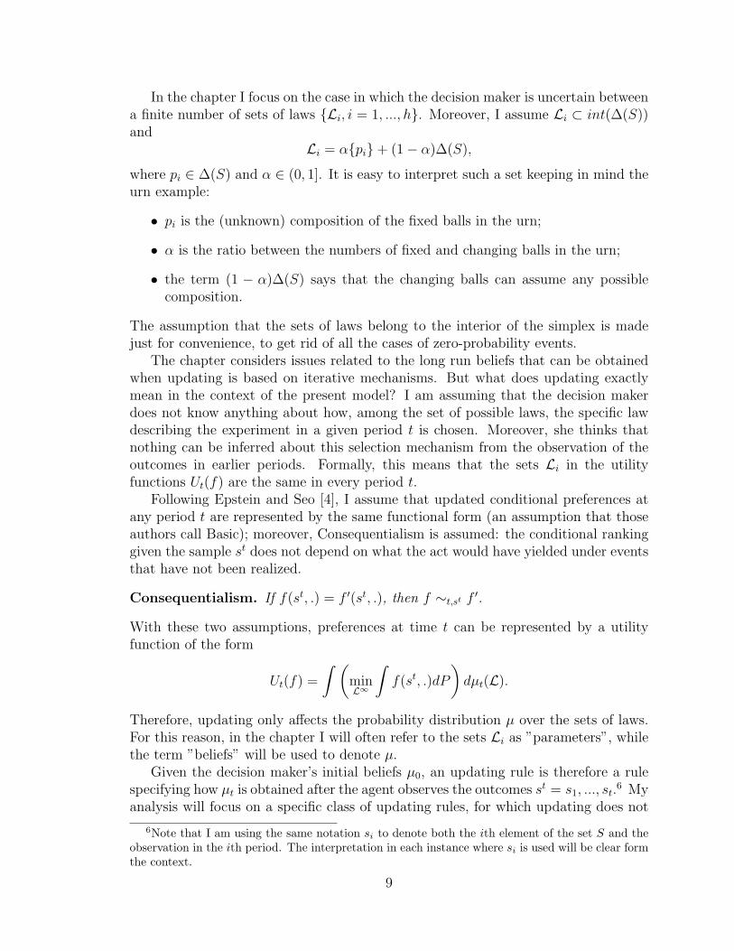
In the chapter I focus on the case in which the decision maker is uncertain betweena finite number of sets of laws Li, i = 1, ..., h. Moreover, I assume Li ⊂ int(∆(S))and

Li = αpi+ (1− α)∆(S),

where pi ∈ ∆(S) and α ∈ (0, 1]. It is easy to interpret such a set keeping in mind theurn example:

• pi is the (unknown) composition of the fixed balls in the urn;

• α is the ratio between the numbers of fixed and changing balls in the urn;

• the term (1 − α)∆(S) says that the changing balls can assume any possiblecomposition.

The assumption that the sets of laws belong to the interior of the simplex is madejust for convenience, to get rid of all the cases of zero-probability events.

The chapter considers issues related to the long run beliefs that can be obtainedwhen updating is based on iterative mechanisms. But what does updating exactlymean in the context of the present model? I am assuming that the decision makerdoes not know anything about how, among the set of possible laws, the specific lawdescribing the experiment in a given period t is chosen. Moreover, she thinks thatnothing can be inferred about this selection mechanism from the observation of theoutcomes in earlier periods. Formally, this means that the sets Li in the utilityfunctions Ut(f) are the same in every period t.

Following Epstein and Seo [4], I assume that updated conditional preferences atany period t are represented by the same functional form (an assumption that thoseauthors call Basic); moreover, Consequentialism is assumed: the conditional rankinggiven the sample st does not depend on what the act would have yielded under eventsthat have not been realized.

Consequentialism. If f(st, .) = f ′(st, .), then f ∼t,st f ′.

With these two assumptions, preferences at time t can be represented by a utilityfunction of the form

Ut(f) =

∫ (minL∞

∫f(st, .)dP

)dµt(L).

Therefore, updating only affects the probability distribution µ over the sets of laws.For this reason, in the chapter I will often refer to the sets Li as ”parameters”, whilethe term ”beliefs” will be used to denote µ.

Given the decision maker’s initial beliefs µ0, an updating rule is therefore a rulespecifying how µt is obtained after the agent observes the outcomes st = s1, ..., st.

6 Myanalysis will focus on a specific class of updating rules, for which updating does not

6Note that I am using the same notation si to denote both the ith element of the set S and theobservation in the ith period. The interpretation in each instance where si is used will be clear formthe context.

9

depend on past observations and beliefs (see Section 1.3). I am interested in particularin the limit beliefs as t → ∞. When is it possible to converge to a probabilitydistribution assigning probability one to the true parameter? Does the answer dependon the cardinality of the set S? These are some of the questions addressed in thefollowing sections.

1.2.2 Differences with Respect to the Epstein-Seo Model

The present model is clearly a special case of the one studied by Epstein and Seo[4]. In fact, I am simply restricting the set of possible parameters, assuming that thedecision maker makes a clear distinction between the features that are common to allthe experiments and those that are specific to each experiment. In the urn example,the agent knows how many balls are fixed in every period and how many change fromperiod to period. This implies that the different sets of laws among which the agentis uncertain can be obtained translating a single set. Formally, two sets of laws candiffer only by the term pi in the expression above. This is not the case for Epsteinand Seo. In their model the decision maker is unsure not only about the colors of thefixed balls, but also about their number.7

To understand why this restriction matters, remember that nothing is knownabout how a specific law is selected in each period. In particular, it cannot be excluded(and the decision maker in my model does not exclude) that in each period one lawin chosen randomly among the laws in the true set.

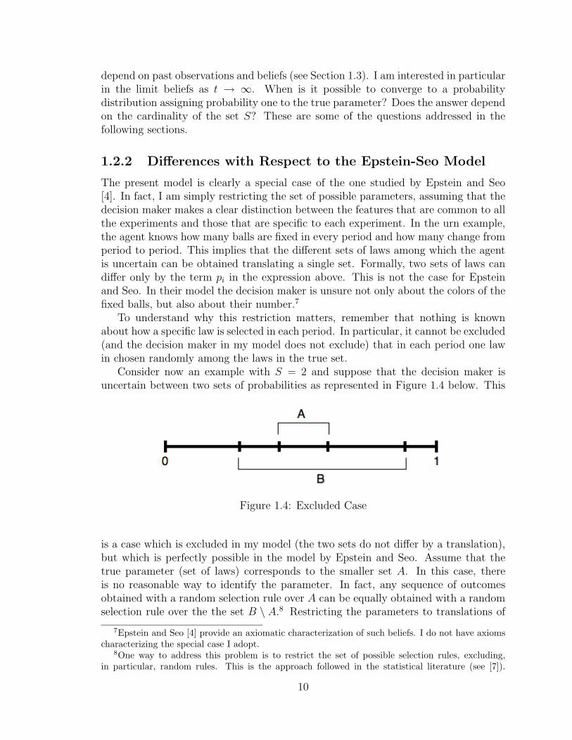
Consider now an example with S = 2 and suppose that the decision maker isuncertain between two sets of probabilities as represented in Figure 1.4 below. This

Figure 1.4: Excluded Case

is a case which is excluded in my model (the two sets do not differ by a translation),but which is perfectly possible in the model by Epstein and Seo. Assume that thetrue parameter (set of laws) corresponds to the smaller set A. In this case, thereis no reasonable way to identify the parameter. In fact, any sequence of outcomesobtained with a random selection rule over A can be equally obtained with a randomselection rule over the the set B \ A.8 Restricting the parameters to translations of

7Epstein and Seo [4] provide an axiomatic characterization of such beliefs. I do not have axiomscharacterizing the special case I adopt.

8One way to address this problem is to restrict the set of possible selection rules, excluding,in particular, random rules. This is the approach followed in the statistical literature (see [7]).

10

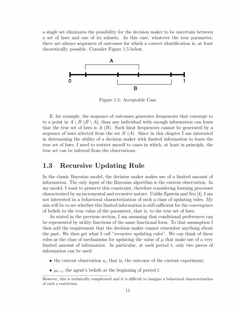
a single set eliminates the possibility for the decision maker to be uncertain betweena set of laws and one of its subsets. In this case, whatever the true parameter,there are always sequences of outcomes for which a correct identification is, at leasttheoretically, possible. Consider Figure 1.5 below.

Figure 1.5: Acceptable Case

If, for example, the sequence of outcomes generates frequencies that converge toto a point in A \ B (B \ A), than any individual with enough information can learnthat the true set of laws is A (B). Such limit frequencies cannot be generated by asequence of laws selected from the set B (A). Since in this chapter I am interestedin determining the ability of a decision maker with limited information to learn thetrue set of laws, I need to restrict myself to cases in which, at least in principle, thetrue set can be inferred from the observations.

1.3 Recursive Updating Rule

In the classic Bayesian model, the decision maker makes use of a limited amount ofinformation. The only input of the Bayesian algorithm is the current observation. Inmy model, I want to preserve this constraint, therefore considering learning processescharacterized by an incremental and recursive nature. Unlike Epstein and Seo [4], I amnot interested in a behavioral characterization of such a class of updating rules. Myaim will be to see whether this limited information is still sufficient for the convergenceof beliefs to the true value of the parameter, that is, to the true set of laws.

As stated in the previous section, I am assuming that conditional preferences canbe represented by utility functions of the same functional form. To that assumption Ithen add the requirement that the decision maker cannot remember anything aboutthe past. We then get what I call ”recursive updating rules”. We can think of theserules as the class of mechanisms for updating the value of µ that make use of a verylimited amount of information. In particular, at each period t, only two pieces ofinformation can be used:

• the current observation st, that is, the outcome of the current experiment;

• µt−1, the agent’s beliefs at the beginning of period t.

However, this is technically complicated and it is difficult to imagine a behavioral characterizationof such a restriction.

11

Notice that, when applied to the non-ambiguous setting, this class includes Bayesrule, among many others.

It is useful to classify recursive updating rules into subgroups. I will consideronly deterministic mechanisms, in which beliefs are updated applying the same rulein each period. Therefore, there exists a function f : (S,∆(Li)) → ∆(Li) suchthat, given the observation st in period t,

µt|st = f(st, µt−1).

In the literature on beliefs updating it is common to focus on mechanisms makinguse of likelihood functions. In the present chapter I use a nonstandard definition: Icall likelihood function any function g : S → Rh

++ such that

(µt|st)i =g(st)iµt−1,i∑

j=1,...,h g(st)jµt−1,j

, i = 1, ..., h.

The difference with respect to the common notion of likelihood function is that I donot require

∑s∈S g(s)i = 1 for all i = 1, ..., h. So, strictly speaking, g cannot be

interpreted as the probability of the current observation given a specific value of theparameter. When I talk about a likelihood function, I am therefore thinking of anyupdating mechanism showing a multiplicative separation of s and µ. Again, Bayesrule is a special case of this class of rules.

It is useful to consider further subsets of mechanisms of the likelihood functiontype. Let Li = αpi+ (1− α)∆(S). We can think of two relevant special cases:

1. Likelihood functions associate to each parameter probabilities belonging to thecorrespondent set of laws: g(s)i ∈ αpi(s) + (1 − α)[0, 1]. We can think ofthese as the only ”meaningful” likelihoods, since, given any outcome and anyparameter, they assume one of the possible values of the conditional probabilityof the outcome given the parameter.

2. Likelihood functions select conditional probabilities that have the same ”posi-tion” within each set of laws: g(s)i = αpi(s) + (1− α)qs(s), where qs ∈ ∆(S) isthe same for all is. So, in the urn example, we can interpret different likelihoodfunctions as different hypotheses on the composition of the variable part of theurn.

Clearly, the second subset of mechanisms is a special case of the first.In the rest of the chapter, I will consider cases in which the decision maker is

uncertain between two possible sets of rules only, L1 and L2; that is, h = 2. Theassumption simplifies the proofs, but does not reduce the power of the theorems. Anyresult can be easily generalized to an arbitrary finite h. A more serious restriction isthe introduction of some mild regularity conditions.

Well-behavedness. Given h = 2, let’s simplify the notation redefining f as a func-tion mapping (S, (0, 1)) to [0, 1], where µ ∈ (0, 1) is now the probability associ-ated to L1. I require that, for any s ∈ S,

12

i) limµ→0 f(s, µ) = 0 and limµ→1 f(s, µ) = 1;

ii) f ′(s, .) has limits (possibly infinite) for µ→ 1 and µ→ 0.

The first condition has a simple interpretation. As beliefs approach certainty, a singleobservation cannot change them dramatically. This is a restriction on the weight thatcan be assigned to observations relative to prior beliefs or, more precisely, a restrictionon the speed with which this weight can increase as beliefs approach certainty. Thesecond condition can be interpreted as an additional restriction on the weights givento observations for different prior beliefs. I assume that, as beliefs approach certainty,these weights don’t oscillate indefinitely. The relevance of observations for updatingbeliefs converges to a singe value, not necessarily finite. Notice that I do not requiref(s, .) to be continuous on the entire interval (0, 1). Observations may in generalbe weighted very differently for arbitrarily close priors. What I need is that thisshould not be the case in the limit; that is, I need f(s, .) to be definitely uniformlycontinuous.

A function f satisfying these conditions will be called ”well-behaved”. Assumingthat f is well-behaved is a significant restriction. The assumption clearly reduces thepower of Theorem 1.4.1 below. In order to prove that the amount of information thatthe decision maker can use in my model is not sufficient for a correct identification ofthe true set of laws, one would like to get rid of these regularity conditions, howevermild they may appear. Whether the same result can be proved for generic functionsf is still an open question.

1.4 Updating Rules and Long Run Beliefs

Before studying the decision maker’s limit beliefs when updating is recursive, I wantto introduce an additional assumption. The assumption will make the similarity withthe standard Bayesian model even stronger. Since experiments are non-identical andnot even independent, there is no guarantee that the frequencies of the outcomesin S will converge in the limit. In the following theorems, however, I will alwaysassume that convergence takes place, in analogy with the model without ambiguity.Informally, we can interpret the experiments as independent ”in the limit”. Noticethat, since my main result will be an impossibility theorem, such a restriction doesnot affect the strength of the result.

I want to study the possibility for the decision maker of learning which of thetwo sets of laws is the true one. However, as we have seen in the Introduction,there are cases that are objectively undecidable. Consider L1 and L2 such thatL1 ∩ L2 6= ∅. Suppose that the relative frequencies of the outcomes converge to apoint in the intersection. Remember that the decision maker does not know anythingabout how a law is selected in each period from the true set. Moreover, she thinksthat any selection mechanism is possible. In particular, a random mechanism cannotbe excluded. For such a decision maker, limit frequencies in L1 ∩ L2 are compatiblewith both sets of laws. This is true no matter how much information she has on thehistory of past observations.

13

On the other hand, if the decision maker were able to observe the frequencies ofthe various outcomes, it would make sense for her beliefs to converge to µ(L1) = 1(µ(L2) = 1) if the limit frequencies belong to the set L1 \ L2 (L2 \ L1). In fact, asequence of outcomes whose limit frequencies fall outside Li cannot be generated by asequence of laws belonging to Li. Clearly, since the decision maker in my model usesa recursive updating rule, she does not have information on the empirical frequencies.This, however, is not a problem in the standard Bayesian case: the true parameterwill be correctly identified in the long run. The question I want to address is whethersuch a result is still possible in the present model, where permanent ambiguity isintroduced. More precisely, I am going to require something a little weaker: I ask fora correct identification of the true set only when limit frequencies fall in int(Li \Lj).As the following theorem shows, even this is generally impossible for well-behavedupdating rules.

Theorem 1.4.1. Suppose S ≥ 4. Let rt(s) be the relative frequency of the outcomes after the first t periods. Let f : (S,∆(Li)) → ∆(Li) be any well-behavedrecursive updating rule. Then, there exist L1, L2, and µ0 ∈ ∆(Li) such that, forsome p ∈ int(L1 \ L2), rt → p but µt 9 δL1.

Theorem 1.4.1 says that, if there are more than three possible outcomes, it may beimpossible for the decision maker to learn the true set of laws, even if the sequence ofobservations is compatible with one of the two sets only. Therefore, the identificationof the true parameter, possible in the standard Bayesian model, does not extend tothe case of permanent ambiguity. This is true, at least, if we restrict ourselves to well-behaved updating rules. The proof of the theorem makes clear that the problems inidentifying the true set arise only when the sets intersect (and not even in all of thesecases).

What is generally not possible when S ≥ 4 becomes possible if S ≤ 3. In thiscase there always exists an updating rule with a likelihood function g such that theparameter L1 (L2) is correctly identified if the limit frequency falls in int(L1 \ L2)(int(L2 \ L1)).

Theorem 1.4.2. Let S ≤ 3 and let the decision maker be uncertain between theparameters L1 = αp1 + (1 − α)∆(S) and L2 = αp2 + (1 − α)∆(S). There exists alikelihood function g : S → ∆(S) such that, if the limit frequency falls in int(L1 \ L2)(int(L2 \ L1)), then the decision maker’s beliefs converge to δL1 (δL2).

It would probably be possible to prove that the likelihood function can be chosensuch that g(s)i ∈ αpi(s) + (1 − α)[0, 1] (the first of the special cases considered inSection 1.3). For the special case in which int(L1)∩ int(L2) 6= ∅, this result is easy toprove, as shown in Appendix A (Remark 1). I have not tried to prove whether thisis true in general.

On the other hand, for S = 3, it turns out that it is not possible to have alikelihood function satisfying the second special case in Section 1.3. In fact, as thefollowing lemma shows, we can find examples where there is no qs ∈ ∆(S) such thatg(s)i = αpi(s) + (1− α)qs(s) for i = 1, 2.

14

Lemma 1.4.1. For S = 3, there exist L1 = αp1 + (1− α)∆(S) and L2 = αp2 + (1−α)∆(S) such that no likelihood functions satisfy both Theorem 4.2 and the conditiong(s)i = αpi(s) + (1− α)qs(s), for i = 1, 2 and qs ∈ ∆(S).

Whether this becomes possible for S = 2 is still an open question.

1.5 Conclusions

In this chapter I have analyzed some issues arising from the problem of updatingbeliefs when the observations come from a sequence of non-identical experiments. Ihave considered the case in which the individual has severe limitations on the amountof information she can carry from one period to the next. In particular, she forgetsall past observations and past beliefs; all she can remember are her beliefs at theend of the previous period. I focused on this special case to preserve an analogywith the classical Bayesian updating model. Moreover, while forgetfulness of all pastobservations can be considered an extreme case, forgetfulness of past beliefs is a verysensible assumption. In particular, the possibility of choosing an updating rule asa function of initial beliefs µ0 assigns to those beliefs a special status that is hardlyjustifiable. In fact, what should be the intrinsic difference between initial beliefs andthose in following periods? Not to mention the fact that in real situations the notionof ”initial period” is ambiguous at best.

To compensate for this limitations, I have restricted myself to a framework that,intuitively, would be the most favorable in order to learn the set of laws that char-acterize the sequence of experiments. Therefore I have considered the case of twoonly possible sets of laws and, within each set, I have assumed that there is a cleardistinction, known by the individual, between what is common to all the laws andwhat changes from law to law. I have also excluded the possibility of sequences ofobservations compatible with both sets of laws. Finally, I have assumed that relativefrequencies converge to a limit distribution.

The main result (Theorem 1.4.1) is an impossibility statement: given the abovelimits on available information, there are no ”well-behaved” updating rules assuringthat beliefs converge in the limit to a distribution that assigns probability one to thetrue set of laws. ”Well-behavedness” is an assumption on the form of the updat-ing function that imposes some regularity conditions in the limit, as the probabilityassigned to one of the sets of laws approaches one.

One weakness of the paper is apparent: Theorem 1.4.1 works under a specificassumption on the class of updating rules we are allowed to consider, namely well-behavedness. It is maybe a weak assumption, but it is still annoying. It would beinteresting to verify whether the theorem holds when this assumption is dropped. Isit true that there are no recursive updating rules, no matter how they behave whenbeliefs approach certainty, that allow the individual to asymptotically identify thetrue set of laws?

Finally, it may be interesting to find general conditions under which identificationis possible. Theorem 1.4.2 states that, when the number of different outcomes is atmost three, beliefs converge to a distribution assigning probability one to the true

15

set of laws. Alternatively, we may ask what minimum amount of information needsto be retained in order to have the same limit result with an arbitrary finite numberof outcomes. Does the individual need to remember all past observations? Is theresome sufficient statistics?

The model of ”objective ambiguity” introduced by Epstein and Seo [4] is surelyworth additional investigation. The present work, and the conclusive suggestions, arejust one of the possible ways to understand its deepest implications.

16

Chapter 2

Updating and Misperception ofSignals

2.1 Introduction

Beliefs updating has generated an immense literature. Several rules (Bayes, General-ized Bayes, Dempster-Shafer, etc.) have been studied and applied to preferences withdifferent utility representations. For recent developments see, for example, Pires [13],Wang [15], Hanany and Klibanoff [11], Eichberger, Grant and Kelsey [2] and Shmayaand Yariv [14]. In these works, the decision maker observes an event or, more gener-ally, a signal. Given this information, she updates her prior beliefs. Looking at theconditional preferences and and having observed the signal, an external observer candetermine the rule the decision maker uses to update her beliefs (or, more precisely,he can model the change in preferences as if the decision maker was updating herbeliefs according to a certain rule). In all these models, the decision maker and theexternal observer see the same signals. But what happens if the decision maker doesnot observe the true signal?

Consider the following example. An urn contains balls with colors in the set S.A ball is drawn and a signal is generated. The signal gives some information on thecolor of the ball: it says that the color belongs to a certain subset of S. If the coloris s, the possible signals can be identified with subsets of S whose elements includes. Assume that, given the true color s, any signal that includes s may be generated.So, for example, the signal s1, s2 can be observed under both states s1 and s2.An external observer is aware of the true signal, but the decision maker is not: herobservational capabilities can be described with a function that assigns to each signalsome other set of colors. This means that, although the decision maker may notobserve the signal correctly, she still interprets signals as subsets of S. Assuming acorrespondence between signals and sets of states is clearly a serious restriction tothe applicability of the model. However, I think that even in this limited settinginteresting questions can be addressed.

Over this structure one can accommodate any kind of updating rules. Giveninitial beliefs and the signal as observed by the decision maker, one can apply any of

17

the updating rules that have been studied in the economic literature. In the presentwork, however, I am only interested in the characteristics of the function mappingeach true signal to what the decision maker perceives. I will introduce assumptions ofthe sort ”given a certain relation between two true signals, the corespondent signalsperceived by the decision maker must satisfy some other relation.” These assumptionsformalize the classes of mistakes that the decision maker can or cannot make. I willthen look at what those assumptions imply in terms of the set of signals that arecorrectly perceived and at how we can restrict the class of perceived signals that thedecision maker may associate to each true one.

Section 2.2 introduces two additional assumptions that will be always maintainedthroughout the chapter. One is a standard non-degeneracy assumption for conditionalpreferences. The other, that I will call Coherence, says that any true signal is mappedinto a subset of S that would be correctly recognized if observed. The idea is thatthere exists a function v : Σ→ Σ such that, after receiving the signal A, the decisionmaker behaves as if she had observed the signal v(A). But this interpretation makessense only if, when the decision maker receives the signal v(A), she correctly perceivesit. Therefore, for any signal A, I require that v(A) is a fixed point of the function v.

Some relations between real and perceived signals can be interpreted as an indi-cation of the level of the decision maker’s confidence on what she observes. So we caninterpret a situation in which A ⊂ v(A) as a case of underconfidence: the decisionmaker does not feel she can exclude all the states of the world that are impossiblegiven the signal. On the other hand, she can be seen as overconfident if v(A) ⊂ A:after receiving the signal A, she is so confident about some of the states of the worldthat she dismisses the others even though the signal does not justify this exclusion.It is tempting to interpret underconfidence as a version of conservatism. However, inthe traditional definition of conservatism, as given by Phillips and Edwards [12], thedecision maker’s updated beliefs lie somewhere between prior beliefs and what wouldbe implied by Bayesian updating. This is not necessarily the case in the presentcontext, in which nothing is assumed about beliefs over conditionally non-null states.

In Sections 2.3 and 2.4 I will study two specific sets of behavioral assumptionsfrom which underconfidence and overconfidence can emerge. In the first model, thedecision maker never excludes any state that is possible under the signal, but maynot be able to distinguish between some states. So the signal she perceives is the onecontaining all the states that are indistinguishable from some state in the true signal.The second model adds a second source of misperception. Some sets of states aremore vivid than others. When the true signal contains a set of states that is morevivid compared to some other state in the signal, this last state is excluded by thedecision maker. These assumptions have some interesting consequences with regardsto the set of fixed points of the function v and to how v(A) is computed for each truesignal A.

Section 2.5 presents some considerations on how the decision maker interpretssignals that differ in the amount of information they provide. In particular, I willanalyze the relation between v(A) and v(B) on one side and v(A ∪ B) or v(A ∩ B)on the other.

Proofs can be found in Appendix B.

18

2.2 Framework

Let S be a finite set of states of the world; Σ, the set of all subsets of S, is the setof events. Let X be the set of outcomes and define acts as functions f : S → Xmapping states of the world into outcomes. L will denote a set of acts and % apreference relation over L.

The decision maker receives a signal providing information on the state of theworld. I am going to distinguish between what an external observer (let’s call it the”experimenter”) can see, and what can be perceived by the decision maker. Theexperimenter observes the signal correctly. Moreover, he knows what the probabilityof any signal is, conditional on each state; that is, he knows the ”true” likelihoodfunction λ. This is not necessarily the case for the decision maker.

Let’s denote with H the set of possible signals. Throughout the chapter I willassume that, for any η1, η2 ∈ H, there exists s ∈ S such that either λ(η1|s) > 0 andλ(η2|s) = 0, or λ(η1|s) = 0 and λ(η2|s) > 0. That is, different signals correspond todifferent subsets of Σ.

For example, imagine a situation in which a ball is drawn from an urn. Thepossible colors of the ball constitute the set of states S. A signal is then generated.The signal gives some information on the color of the ball: it says that the colorbelongs to a certain subset of S. Given the state s, the set of possible signals can beidentified with a subset of S whose elements include s. Assume that, for any signaland for any s included in it, the likelihood of observing the signal given s is positive.So, for example, the signal s1, s2 can be observed under both states s1 and s2. Suchan example satisfies the assumptions of my model.

Notice that the decision maker may have a wrong belief on how signals are gen-erated given states; or she may be unable to distinguish between different signals.However, I will always assume that the decision maker associates signals with subsetsof S, so that different signals (according to what she can perceive) correspond todifferent subsets. This will imply that conditional beliefs can be identified with a setof conditionally non-null states. That is, there cannot be two different conditionalbeliefs that share the same set of non-null states.

The framework can accommodate decision makers with various ways of misin-terpreting the signals. In the chapter I will consider some behavioral assumptionsthat may seem quite reasonable, and I will ask what class of updating mechanismsdescribes a decision maker behaving in this way.

Let’s formalize the above discussion, redefining the properties in terms of prefer-ences. Given the correspondence between signals and elements of Σ, in what follows Iwill use the same notation for both signals and events. The meaning in each instancewill be clear from the context. Therefore, the symbol %A denotes the preference re-lation conditional on the signal corresponding to the set A. Notice that this is the”true” signal, that is the one observed by the experimenter. I will also focus on thespecial case in which H = Σ, that is, for any subset of S there exists a correspond-

19

ing signal.1 As I said, I want to assume that even for the decision maker there isan analogous relation between signals and events. Formally, this corresponds to thefollowing assumption.

A1 (Signals as events) For any A,B ∈ H, if the set of %A-non-null events is equal tothe set of %B-non-null-events, then, for any f, g ∈ L, f %A g ⇐⇒ f %B g.

When the decision maker observes the signal E, she interprets it as saying thatsome events are impossible. So she divides Σ into two groups of conditionally nulland non-null events. It is this reformulated information that enters the updatingmechanism, so that the new preferences %E are completely characterized by theset of %E-non-null events. The axiom excludes the existence of different conditionalpreferences %A and %B sharing the same set of conditionally non-null events. Thanksto Axiom 1, we can represent the updating rule with a function v : Σ→ Σ mappingeach signal into the corresponding set of conditionally non-null states of the world.

The role of Axiom 1 is to limit the class of updating rule under consideration. Icannot exclude that my approach could generalize to a more general set of rules. Theaxiom, however, is reasonable enough not to obliterate the interest of the results inthis limited setting.

In the chapter I will always consider updating rules that satisfy an additionalaxiom, that I call ”Coherence”.

A2 (Coherence) Given any signal E, let E ′ be the set of %E-non-null states, that is,for any F ⊆ E ′, ∃f, g, h ∈ L such that f |hF c E g|hF c , where f |hF c denotes anact that coincides with f on F and with h on F c. Then, E ′ is also the set of%E′-non-null states.

In other words, Axiom 2 states that the function v maps any signal into a fixedpoint: ∀E ∈ Σ, v(v(E)) = v(E). Notice that, up to this point, I have not made anygeneral assumption on the relation between E and v(E). It may well be the casethat, for some signal E, v(E) ⊂ E, or E ⊂ v(E), or that E and v(E) intersect in amore generic way. It may even be the case that E and v(E) are disjoint.

The reason for calling this property ”coherence” is obvious. Consider a signalA and let B be the set of %A-non-null states. We can say that, after receiving thesignal A, the decision maker behaves as if she has observed the signal B. If this isthe interpretation, it must be the case that the decision maker can correctly perceivethe signal B.

Finally, I add the standard requirement that conditional preference are non-degenerate.

A3 (Non-degeneracy) For any E ∈ Σ, ∃f, g ∈ L : f E g.

Axioms 1-3 lead to the following simple result.

1Results similar to those obtained in the chapter may hold in the more general case in whichH ⊆ Σ. However, axioms must be modified to adapt to the new setting.

20

Proposition 2.2.1. Given Axiom 1, conditional preferences satisfy Axioms 2 and 3if and only if there exists a unique collection V of sets such that:

(i) For any V ∈ V and for any E ∈ Σ, E is %V -non-null if and only if E ∩ V 6= ∅;

(ii) For any E ∈ Σ, ∃! V E ∈ V such that ∀f, g ∈ L, f %E g ⇐⇒ f %V E g.

Property (i) defines V as the set of fixed points of the function v. Setting V E =v(E), Proposition 2.2.1 is just a different way to express coherence.

2.3 Indistinguishable Signals

Imagine a decision maker who cannot distinguish between two or more signals. Whatmay be a plausible reason? An interesting possibility is given by the following axiom.

A4 (Strong Indistinguishability) Given a signal A ∈ Σ and a state s ∈ S,(∃f, g ∈ L with f(s′) = g(s′), ∀s′ 6= s s.th. f A g

)⇐⇒

(∃s′′ ∈ A s.th. ∀f, g ∈ L, f %s g ⇐⇒ f %s

′′ g).

The axiom says that, given a signal A, a state s is conditionally non-null if andonly if there exists a state s′′ ∈ A such that the decision maker cannot distinguishbetween the signals s and s′′. Notice that I call two signals indistinguishablewhen updated preferences are the same conditional on any of them.2 Consider thefollowing example. An urn contains red, yellow, and black balls: S = r, y, b. Thedecision maker can correctly observe the color yellow, that is v(y) = y, but shecannot distinguish red from black: v(r) = v(b) = r, b. Suppose a ball is drawnand the decision maker receives a signal r, y, corresponding to the event ”the ball iseither yellow or red.” By Axiom 4, she must consider all three colors as possible. Notonly cannot the colors corresponding to the ”true” signal be excluded, but the samemust hold for any color indistinguishable from one of them. So v(r, y) = r, y, b.

Notice that Axiom 4 implies that all the states contained in a signal are non-null.Moreover, if there exists a signal E such that v(E) 6= E, the decision maker satisfieswhat I call ”global underconfidence”, as formalized in the following definition.

Definition 2.3.1 (Underconfidence). Given the event A ∈ Σ, the decision maker isweakly underconfident if, for any B ⊆ A, ∃f, g, h ∈ L such that f |hBc A g|hBc . If,in addition, there exists a set C with A ∩ C = ∅ satisfying the same property, thedecision maker is said to be underconfident. She is globally underconfident if she isweakly underconfident for any signal in Σ and underconfident for some signals.

2In what follows, I will say that two states are indistinguishable when the corresponding singletonsare.

21

The question now is what kind of updating rules correspond to such an assumption.That is, I want to find the properties of the set of fixed points of v and to determinehow, given a signal, conditional non-null states can be computed. The answer is givenby the following proposition.

Proposition 2.3.1. Given Axiom 1, conditional preferences satisfy Axiom 4 if andonly if there exist a unique set V ⊆ Σ such that (i) and (ii) in Proposition 2.2.1 holdand

(iii) for any signal E ∈ Σ, E ⊆ V E and @ V ∈ V : E ⊆ V ⊂ V E;

(iv) V ∪ ∅ is an algebra.

Notice that Axiom 4 implies both Coherence and Non-degeneracy, as is clear fromthe comparison of Propositions 2.2.1 and 2.3.1.

2.4 Dominated States

t may be interesting to look for updating rules which do not imply that the decisionmaker is always underconfident. In fact, it is not unreasonable to allow for signalsafter which she shows overconfidence, a behavior defined as follows.

Definition 2.4.1 (Overconfidence). Given the event A ∈ Σ, we say that the decisionmaker is overconfident if

(i) there exists no B with A ∩B = ∅ such that ∃f, g, h ∈ L with f |hBc A g|hBc ;

(ii) there exists some C ⊂ A such that, for any f, g, h ∈ L, f |hCc ∼A g|hCc .

Simply put, overconfidence consists in the set of conditionally non-null states beinga subset of the signal. What may be a reason for overconfidence? We can imaginethat some event is so more vividly perceived by the decision maker compared tosome other state, that, every time the signal does not exclude that event, the decisionmaker disregard the other state. In the urn example, suppose that the decision makeris so much impressed by the color red and so little but the color yellow that, whenred is possible, she does not pay attention to the possibility of the drawn ball beingyellow. So, for example, we have v(r, y) = r. This intuitive argument has animportant implication: if, given the signal A, vividness considerations exclude states ∈ A, then the same s must be excluded given any signal B such that A ⊂ B. Infact, if s is excluded because it’s ”dominated” by some event E ⊂ A (that is, becauseE is ”more vivid” than s), it must be excluded also given B, since E ⊂ B. Moreover,it is consistent with the intuition of relative vividness to assume that all states thatare excluded from a signal are dominated by some set of conditionally non-null states.The restriction here is the requirement that the ”dominating” states be conditionallynon-null. This behavior is formally described in the following axiom.

A5 (Relative vividness) Given a signal A, let B be the set of conditionally non-nullstates (as defined in Axiom 2). Then for any s ∈ A \B

22

(i) for any f, g ∈ L, f %B g if and only if f %B∪s g;

(ii) for any signal A′ such that A ⊂ A′, s is %A′-null.

Notice that Axiom 5 does not say that any %A-null state s must also be %B∪s-null. This property has to hold just for s ∈ A. We can interpret (ii) as a sortof confidence monotonicity: the decision maker is relatively more confident for lessinformative signals. This must be interpreted in a very weak way, though. It isnot necessarily the case that overconfidence for A implies overconfidence for any A′

such that A ⊂ A′. However, if the decision maker is so ”confident” that she canexclude some objectively possible state conditionally on a signal, she will still showthis ”confidence” conditionally on any less informative signal.

We can imagine a decision maker characterized by both ”relative vividness” and”indistinguishability”. Given a signal A, if she does not exclude some state s /∈ A,the reason is that she cannot distinguish s from some s′ ∈ A. On the other hand,if she exclude some s′′ ∈ A, it means that the set of conditionally non-null state ismore ”vivid” than s′′. To describe such a decision maker we need to add the followingaxioms.

A6 (Indistinguishability) Given a signal A and given s /∈ A such that ∃f, g, h ∈ Lsuch that f |hsc A g|hsc , there exists s′ ∈ A such that, ∀f, g ∈ L, f s g if andonly if f s′ g.

Axiom 6 says that if, given a signal A, some state s not included in A is condi-tionally non-null, then there there must exists a state in A that the decision makercannot distinguish from s. Notice that this axiom is weaker than Axiom 4. Here weallow for the possibility that states indistinguishable from a state in A may still beconditionally null. A difficulty arises from the interaction of Axioms 5 and 6. It mightbe the case that some state s′ /∈ A is non-null because indistinguishable from somes ∈ A, but s is null because of vividness considerations. To exclude this possibility, Iintroduce an additional axiom.

A7 (Equi-vividness) Given a signal A, let the states s ∈ S and s′ ∈ A be such that∀f, g ∈ L, f s g if and only if f s′ g. Then ∃f, g, h ∈ L such thatf |hsc A g|hsc if and only if the same is true for s′.

Axiom 7 makes two requirements. On one hand, it says that if a state s ∈ A isconditionally non-null, then the same must be true for all the states that the decisionmaker cannot distinguish from s.3 On the other hand, if s is null (because some otherevent is more vivid), all the indistinguishable states must be null, too. Informally, Iwant that indistinguishable states share the same vividness properties.

What kind of updating rules are implied by these axioms? The following propo-sition provides a result.

3This implies that, for states in A that are conditionally non-null, the converse of Axiom 6 holds.

23

Proposition 2.4.1. Given Axioms 1 and 5, conditional preferences satisfy Axiom 2,3, 6 and 7 if and only if there exists a unique set V ⊆ Σ such that (i) and (ii) inProposition 2.2.1 hold and

(iii) V ∪ ∅ is a semialgebra; moreover, ∀A,B ∈ V , A \B ∈ V ∪ ∅.

(iv) for any A ∈ Σ, V A satisfies the conditions:

1. V A ∩ A 6= ∅;2. V A ∩ A 6⊂ V ∩ A, ∀ V ∈ V;

3. V A ⊆ V, ∀ V ∈ V s.th. V ∩ A = V A ∩ A.

Given V and a signal A, property (iv) provides the restrictions that must be satis-fied by the set of %A-non-null states. Notice that the proposition implies that, givena signal A, if V contains supersets of A, then V A is the smallest of these supersets,where existence of a smallest superset is guaranteed by closure under intersection.A weakness of Proposition 2.4.1 is the absence of a sufficient condition for Axiom 5.Finding it is not a trivial task. In Proposition 2.3.1, there is a clear rule associatingeach signal to the set of conditionally non-null states. This set can be determinedindependently for each signal. Here, on the other hand, a single set V may allow fordifferent preference relations: for many signals, there are multiple sets of condition-ally non-null sets that are compatible with V . Of course, not all the sets satisfying(iii) and (iv) above can be taken: the choice of V A for some signal A constrains thecorrespondent choice for other signals. However, this is not a restriction that can beincluded in the proposition: it would be nothing more that a re-statement of Axiom5.

The following corollary establishes a relation between the classes of indistinguish-able signals and the respective sets of conditionally non-null states.

Corollary 2.4.1. Take V ∈ V and let A1, ..., Ak be all the signals such that

• V Ai = V ;

• there is no signal B ⊂ Ai such that V B = V .

Given Axiom 1, if conditional preferences satisfy Axiom 2, 3, 5-7, then V =⋃ki=1 Ai.

2.5 Response to Information Increases

We have seen that the general model can accommodate for updating rules with verydifferent properties. The same is true with respect to the problem of information ac-quisition. For example, the model is compatible with a setting in which ”objectively”less informative signals provide more information to the decision maker. Consider thefollowing example. There is an urn with red, yellow and green balls; so S = r, y, g.The function v is as follows:

v(y) = y v(r, y) = r, y v(y, g) = y, g24

v(r) = v(g) = v(r, g) = v(r, y, g) = r, y, g.

We can imagine that the decision maker is normally sleepy, and expects an alarmclock to ring when a signal arrives. However, the alarm clock works only if the signaldoes not exclude the color y. When asked to make her choice, a decision makerwho did not hear the alarm believes that no signal arrived. The result is that, forexample, the more informative signal r does not provide any information to thedecision maker, while the less informative r, y gets identified.

Let’s now introduce a new axiom.

A8 (Information monotonicity) Given A,B ∈ Σ, if for any f, g, h ∈ L, f |hBc ∼A g|hBc ,then for any A′ ⊂ A, f |hBc ∼A

′g|hBc .

Axiom 8 states that if an event is null conditionally on a given signal, it must stillbe null conditionally to more informative signals.

In this section I will consider only updating rules that exhibit global undercon-fidence. Therefore, the following propositions do not provide a complete axiomaticcharacterization of classes of updating rules. They say that, given a globally un-derconfident decision maker, if we add some requirement on the way information isacquired, the updating rule exhibits some additional features. The following propo-sition shows the implications of Information monotonicity.

Proposition 2.5.1. Given the representation as in Proposition 2.2.1 and global un-derconfidence, conditional preferences satisfy Axiom 8 if and only ∀A ∈ Σ, there isno V ∈ V such that A ⊆ V ⊂ V A. Moreover, if Axiom 8 holds, then V is closedunder intersection.

Notice that V may be closed under intersection even if v does not satisfy mono-tonicity. It is also evident that Axiom 4 implies Information monotonicity.

More generally, the basic model allows for updating rules that exhibit non-constantreturns to information. This is the interpretation I give to the behavior of the functionv with respect to the union of signals. In general, given two signals A and B, thereare no constraints on the relation between v(A) and v(B) on one side and v(A ∪ B)on the other. Consider the following example. Let S = r, y, g, b and suppose

v(r) = r, g v(y) = y, g v(r, y) = r, y, b,

while all the other signals are fixed points of v. The example clearly satisfied theassumptions in Proposition 2.2.1. However, neither v(r, y) ⊆ (v(r) ∪ v(y)),nor (v(r) ∪ v(y)) ⊆ v(r, y). I say that the updating rule exhibits increasingreturns to information if, for any signals A and B, (v(A) ∪ v(B)) ⊂ v(A ∪ B). Theidea is that when ”objective” information increases (as when we move from the signalA ∪ B to either A or B), the amount of information that the decision maker retainsincreases ”more than proportionally”: both the signals A and B allow the decisionmaker to exclude some event that is not excluded when she receives the signal A∪B.Analogously, I say that the updating rule exhibits decreasing returns to informationif, for all signals A and B, v(A ∪ B) ⊂ (v(A) ∪ v(B)). In this case, when moving to

25

a more informative signal, the decision maker may loose some information she wasable to retain before (which does not mean she cannot at the same time acquire newinformation as well). Finally, if, for any signals A and B, v(A ∪B) = (v(A) ∪ v(B)),I say that there are constant returns to information.

The following axiom reformulates the property of decreasing or constant returnsin terms of preferences.

A9 (Non-increasing returns to information) For any A,B,C ∈ Σ, if ∀f, g, h ∈ L,f |hCc ∼A g|hCc and f |hCc ∼B g|hCc , then f |hCc ∼A∪B g|hCc .

The following proposition analyzes the relation between Axiom 8 and Axiom 9.

Proposition 2.5.2. Given the representation as in Proposition 2.2.1, conditionalpreferences satisfy Axiom 8 if and only if the updating rule exhibits increasing orconstant returns to information. If, in addition, global underconfidence is assumed,then:

(i) if conditional preferences satisfy Axiom 9, then V is closed under union;

(ii) if V is closed under complements and Axiom 8 holds, then the updating ruleexhibits constant returns to information.

Remark 1. Notice that the behavioral hypotheses introduced in this section implysome structural properties on V , but they are not equivalent to them: Informationmonotonicity implies closure under intersection, while Decreasing returns to informa-tion lead to closure under union. The inverse implications do not hold. So in part(ii) it can be easily shown that constant returns to information are not implied ifwe substitute Axiom 9 for Axiom 8; that is, they are not a consequence of V beingan algebra. It would be nice to find a characterization of the structural propertiesthemselves. However, this does not seem to be possible, unless we directly assumethe properties (which can clearly be defined in behavioral terms).

Finally, no more general axiom seems to imply closure under complements. Inparticular, constant returns to information do not imply that V is an algebra.

2.6 Conclusions

This chapter has introduced a new framework to look at phenomena of under- andoverconfidence. Although quite simple, it allows to link confidence considerations tomisperception issues. In particular, I have considered the cases of indistinguishablestates and of vividness comparisons. The abstract nature of the framework can bea limit to its applicability, but it has the advantage of providing concepts and toolsthat can be used in more structured environments.

The emergence of some sort of confidence monotonicity seems to be one of thecentral questions that can be asked using my framework for under- and overconfi-dence. Can we claim that the level of confidence depends on how much informationa signal provides? It would be interesting to be able to say that a decision maker

26

is, in some sense, less confident for more informative signals than for less informativeones. That is, I would like to have a decision maker who, when she receives a lot ofinformation, tends to discard some of it; on the other hand, when she receives little,she may view the signal as more informative than it actually is. In Section 2.4, Ihave assumed a weak form of such a monotonicity and I have provided a rationale forsuch a hypothesis. However, the present chapter does not address the question in asatisfying way. Nevertheless, I think it introduces the formal tools that will make itpossible to look for a more complete answer. What we need is to construct a modelin which confidence monotonicity emerges as a property of endogenously generatedunder- and overconfidence.

A first step towards such a model is provided by next Chapter, in which I builda model in which underconfidence and overconfidence are not assumed, but emergeendogenously.

27

Chapter 3

Optimal Underconfidence andOverconfidence

3.1 Introduction

Imagine a finite set of states of the world and suppose that an individual is uncertainabout which of the states is the true one. Her beliefs can be represented with a proba-bility distributions over the states. Suppose now that, before making her decision, shereceives a signal. This signal provides a particular kind of information: it limits theset of states that can be realized, but it does not provide any additional informationon the probability of the the states that are not excluded. We can therefore representsuch signals as sets of states of the world. The individual, however, may misperceivethe signal she has received, interpreting it as a set (of states) possibly different fromthe real one. She then updates her prior as if she has received this second signal.

What I have just described is the framework that I have introduced in Chapter2. There, I imagine an external observer who can correctly observe the signal, butwho does not know what signal the individual has actually perceived. Observing herbehavior, he wants to determine the nature of the perceiving mistakes that she ismaking. Within this framework, it is possible to define notions of underconfidenceand overconfidence in terms of relations between true and perceived signals. Theindividual exhibits underconfidence if the perceived signal is a superset of the trueone; she is overconfident when the perceived signal is a subset of the one she hasreceived.

The present chapter introduces a model in which the previous concepts may foundan application. The main idea is the following. A decision maker has to choose howto allocate a unit among the different states of the world. If a state is realized, shewill win the fraction that she has allocated to that state. For simplicity, assume thatshe is an expected utility maximizer, with a prior on the probability of the differentstates. Before making her choice, the decision maker receives a signal of the kinddescribed above. The decision maker’s beliefs include the likelihoods of the signalsconditional on each state of the world. After receiving the signal, she updates herprior and chooses the allocation that maximizes expected utility.

28

There is, however, a complication. The decision maker is constrained in the num-ber of different signals she can perceive. The constraint can be interpreted as aboundary on her computational capabilities. Each signal she may receive is inter-preted as one of the signals she can actually perceive. The decision maker’s beliefsare updated through Bayes rule given the actually perceived signal, not the one shetruly receives.

Up to this point the model adds little to the framework in Chapter 2. The funda-mental difference is the existence of an ex-ante stage. Ex ante, that is before receivingthe signal, the decision maker knows that the number of possible true signals is higherthan that of the signals she can distinguish. Given this computational constraint, shewants to choose the set of perceivable signals and the mapping from true signals toperceived ones that maximize her ex-ante expected utility.

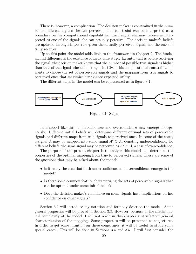
The different steps in the model can be represented as in figure 3.1.

Figure 3.1: Steps

In a model like this, underconfidence and overconfidence may emerge endoge-nously. Different initial beliefs will determine different optimal sets of perceivablesignals and different maps from true signals to perceived ones. In some of the cases,a signal A may be mapped into some signal A′ ⊃ A, denoting underconfidence; fordifferent beliefs, the same signal may be perceived as A′′ ⊂ A, a case of overconfidence.

The purpose of the present chapter is to analyze this model and determine theproperties of the optimal mapping from true to perceived signals. These are some ofthe questions that may be asked about the model:

• Is it really the case that both underconfidence and overconfidence emerge in themodel?

• Is there some common feature characterizing the sets of perceivable signals thatcan be optimal under some initial belief?

• Does the decision maker’s confidence on some signals have implications on herconfidence on other signals?

Section 3.2 will introduce my notation and formally describe the model. Somegeneral properties will be proved in Section 3.3. However, because of the mathemat-ical complexity of the model, I will not reach in this chapter a satisfactory generalcharacterization of the mapping. Some properties will be presented as conjectures.In order to get some intuition on these conjectures, it will be useful to study somespecial cases. This will be done in Sections 3.4 and 3.5. I will first consider the

29

easiest possible case, that with only two states of the world. However, the analysis ofthis case will provide little insight on the properties of the mapping function. Moreconsiderations will be possible in the slightly more complicated case of three statesof the world. The computational details of the analysis will be presented separatelyin Appendix C. Section 3.6 will contain some conclusive considerations.

3.2 The Model

Let S = s1, ..., sn be a finite set of states of the world. Σ, the set of all subsets ofS, is the set of events. A decision maker has a prior probability distribution µ overstates. I limit the set of acts to all the possible allocation of one unit among the nstates. Formally, if the set X of consequences is the set of non-negative real numbersmaller or equal to 1, an act is any function f : S → X such that

∑s∈S f(s) = 1. Let

F be the set of these acts. The decision maker is an expected utility maximizer withvon Neumann-Morgenstern utility index u : X → R, where u is increasing in X andstrictly concave.

Before making her choice, the decision maker receives a signal providing infor-mation on the true state of the world. More specifically, the signal limits the set ofstates that can be realized, but it does not provide any additional information onthe probability of the the states that are not excluded. Therefore, each signal can beassociated to an element of Σ: the true state of the world is one of those contained inthe set. Moreover, I assume that any set in Σ describe a possible signal. With thisassumption, I can use the same notation to denote both events and signals.

Let’s now be more formal on the nature of the signals. The decision maker as-sociates to the signals a likelihood function, which specifies the probability of eachsignal conditional on each state of the world. I will denote with ps(A) the probabilityof signal A conditional on the state s. The interpretation of signals as sets of states, asdescribed above, is equivalent to the following assumptions on the likelihood function:

1. ∀A ∈ Σ, ps(A) > 0 =⇒ s ∈ A;

2. ∀A ∈ Σ, ∀s, s′ ∈ A, ps(A) = ps′(A).

The first assumption says that signals must be truthful: if the signal A can be gener-ated when the true state is s, then A must include s as one of the possible true states.The second assumption assures that no additional information is obtained from thesignal other than the restriction of the set of possible states. It implies that, whenupdating the prior µ through Bayes rule, for any couple of states in A the ratio ofthe posterior probabilities is the same as the ratio of the priors. In addition, I willalso assume that

3. ∀A ∈ Σ, s ∈ A =⇒ ps(A) > 0,

so that, conditional on the state s, any signal that does not exclude s can be generated.

30

Given these assumption, the notation can be simplified noting that

ps(A) =

p(A) > 0 if s ∈ A0 if s /∈ A

To easily follow the rest of the construction of the model, keep in mind Figure 3.1and its description in the Introduction. In the second stage of the decision process,before the decision maker chooses an act, the received (true) signal is mapped intoa perceived signal. Let V ⊂ Σ be the set of perceivable signals. The true signalis interpreted as one of the sets in V . Let v : Σ → V be the mapping function.Therefore, after receiving a signal A, the decision maker actually perceives the signalv(A). She then updates her prior, using Bayes rule, as if she had received v(A). Afterthis, she chooses the act that maximizes expected utility.

The set V and the function v are not exogenously given. Before receiving thesignal, in the first stage of the decision process, the decision maker knows that thereis a limit in the number of different signals she can perceive. Let V denote suchupper limit. V and the decision maker’s beliefs (prior and likelihoods) are the onlyexogenous parameters in the model. The decision maker knows that, in the secondstage, she will behave as described in the previous paragraph. Ex ante, she wants tochoose the set V , with at most V elements, and the function v that, given her priorµ and likelihoods p(·), maximize her expected utility.

The optimization problem can be expressed formally as follows. In the secondstage, after receiving a signal A, the decision maker solves

maxf∈F

∑s∈S

u(f(s))µ(s|v(A))

where µ(s|v(A)) =

ps(v(A))µ(s)∑s′∈S ps′(v(A))µ(s′)

Since

µ(s|v(A)) =

µ(s)P

s′∈v(A) µ(s′)if s ∈ v(A)

0 if s /∈ v(A)

the problem can be simplified to

maxf∈F

∑s∈v(A)

u(f(s))µ(s)

Let f ∗(v,A) be the act that solves the problem. Since u is increasing and strictly

concave, f ∗(v,A)(s) = 0 for any s /∈ v(A) and f ∗(v,A)(s) > 0 for any s ∈ v(A). From anex-ante point of view, the expected utility that the decision maker gets after receivingthe signal A and given the map v is

EU(v, A) =∑s∈S

u(f ∗(v,A)(s))µ(s|A)

31

or, equivalently,

EU(v, A) =1∑

s′∈A µ(s′)

∑s∈A

u(f ∗(v,A)(s))µ(s)

In the first stage, the decision maker chooses a function v such that the cardinalityof v(Σ) is V , in order to maximize the ex ante expected utility. Let vV denote theset of functions v satisfying the cardinality requirement. The problem to solve is then

maxv∈vV

∑A∈Σ

(EU(v, A)

∑s∈S

ps(A)µ(s)

)

or, equivalently, simply

maxv∈vV

∑A∈Σ

(EU(v, A)

∑s∈A

p(A)µ(s)

)

Although quite intuitive, the model is computationally cumbersome even for smallnumbers of states. However, some general properties can be proved, as shown in thenext section.

3.3 General Results and Conjectures

3.3.1 Properties of optimal sets VNot all possible sets V can be optimal for some initial beliefs. The following propo-sition states a property that can be easily proved.

Proposition 3.3.1. When V = 1, the function v such that v(E) = S for all E ∈ Σis always optimal.

Proof is straightforward: when updated beliefs are the same no matter the signalreceived, the optimal thing to do is to consider the signals uninformative; that is, tobehave as if S has been received.1 For generic values of V , other restriction likelyapply. At the present stage I do not have proofs for these properties. However, theanalysis of the case with three states of the world, described in Section 3.5 supportthe following conjectures. The first one can be seen as a generalization of Proposition3.3.1 for the case of generic V .

Conjecture 3.3.1. For any initial beliefs, there exists an optimal set V of observablesignals such that

⋃E : E ∈ V = S. If u′(0) =∞, then a set V can be optimal only

if it satisfies this property.

1Such v is the only optimal mapping if the decision maker is sufficiently risk averse, so that sheallocates to each state of the world a positive share of the unit.

32

Is it the case that any V satisfying this property can be optimal for some initialbeliefs? The analysis in Section 3.5 seems to exclude this possibility. On the otherhand, it may support an additional conjecture.

Conjecture 3.3.2. Let u′(0) = ∞. Any set V such that⋃E : E ∈ V = S can be

optimal for some initial beliefs, unless S /∈ V and there exists a state s such that, forany V ∈ V, s ∈ V .

In fact, with three states of the world, the only set that apparently cannot beoptimal is V = s1, s1, s2, s1, s3.

3.3.2 Properties of optimal functions v

There are other properties of optimal functions v that can be proved, which do nottranslate immediately into features of the set V . First, it is immediate to see thatthere always exists an optimal function v mapping any signal into some fixed pointof v itself. This property was called Coherence in Chapter 2. Its interpretationis straightforward: any signal in the set V of perceivable signals can be correctlyobserved when received.

Proposition 3.3.2. Given any prior µ, likelihoods p and utility index u(.), thereexists an optimal mapping v such that, for any E ∈ Σ, v(E) = v(v(E)).

Proof. Consider a mapping v such that there exists a signal A ∈ Σ such that v(A) 6=v(v(A)). Consider now the map v′ defined as

v′(E) =

v(E) if E 6= v(A)

v(A) if E = v(A)

Notice that EU(v′, v(A)) ≥ EU(v, v(A)), while EU(v′, E) = EU2(v, E) for any E 6=v(A). Denote with Vv the set V corresponding to the function v. It is clear thatVv′ ⊆ Vv, so that v′ continues to satisfy the constraint on the cardinality of V . Thisis enough to prove the result.

Assuming that Conjecture 3.3.1 be true, it is easy to verify that there alwaysexists an optimal v such that, for any received signal E, the corresponding perceivedsignal v(E) must include some of the states in E. The next proposition formulatesthis property in more general terms.

Proposition 3.3.3. For any E ∈ Σ, if there exists a set V ∈ V such that V ∩E 6= ∅,then there is an optimal mapping v for which v(E) ∩ E 6= ∅.2

Proof. Consider a mapping v such that there exists a signal A such that v(A)∩A = ∅.Let V ∈ V be such that V ∩ A 6= ∅. Consider now the map v′ defined as

v′(E) =

v(E) if E 6= A

V if E = A

2Notice that the hypothesis would be satisfied if Conjecture 3.3.1 were true.

33

Notice that EU(v′, A) ≥ EU(v, A), while EU(v′, E) = EU(v, E) for any E 6= A.Moreover, Vv′ = Vv. This proves the result.

Following the approach in Chapter 2, we can define the concept of underconfidenceand overconfidence. The decision maker is underconfident given the signal E whenv(E) ⊃ E; she is globally underconfident when, for any signal E, v(E) ⊇ E and theinclusion is strict for some signal. Similarly, the decision maker exhibits overconfi-dence given the signal E when v(E) ⊂ E; she is globally underconfident when, forany signal E, v(E) ⊆ E and the inclusion is strict for some signal. An underconfi-dent decision maker does not ”trust” the information received: she behaves as if shehas observed a signal less informative than the one received; that is, one including asuperset of the states. Overconfidence is the opposite situation: the decision makerinterprets the signal as more informative than it really is, excluding some states of theworld that, according to the received signal, should be considered possible. Clearly,we can also think of a function v such that, for some signal A, v(A) is neither asuperset nor a subset of A. In this case, the decision maker is neither under- noroverconfident.

The present model is compatible with both underconfidence and overconfidence.It will be shown in Section 3.4 that both behaviors can emerge endogenously from theoptimization problem. Which behavior is observed depends on the decision maker’sinitial beliefs (prior and likelihoods).

3.3.3 Further observations

It may be interesting to verify whether the optimal functions v have to satisfy someconditions that could be interpreted as fixed patterns underlying the misperceptionof signals. Unfortunately, it will be shown that the model does not generally supportsuch patterns. Some useful consideration can however be obtained from these negativeresults.

It has been experimentally shown that people tend to be overconfident in theinformation they possess when facing difficult tasks; their confidence level declinesfor easier ones, possibly leading to underconfidence. See, for example, Lichtensteinand Fischhoff 1977 [8], Griffin and Tversky 1992 [10], or Erev, Wallsten, and Budescu1994 [5]. In the context of the present model, we can consider the choice of theoptimal act as a simple task when the signal received is very informative, and as amore difficult one when the signal is less informative. It would be a nice feature ofthe model if the confidence that the decision maker shows on a signal decreased asthe information it conveys increases. There is not a unique way to formalize this idea.One possibility is to require that, given two signals A and A′, with A′ ⊂ A, and givena state s ∈ A′ such that s /∈ v(A′), it cannot be the case that s∪(A′∩v(A′)) ⊆ v(A).That is, if the decision maker, after receiving the signal A′, is so confident that sheexclude the state s ∈ A′, then she must be at least as confident when receiving theless informative signal A. We can call this property ”Monotone overconfidence”.3

3This property is a weakening of the second point in the definition of Relative vividness, asintroduced in Chapter 2.

34

Does the decision maker in the present model exhibit Monotone overconfidence?In general, this turns out to be false, as shown by the following example.

Example 3.3.1. Suppose that S = s1, s2, s3. As explained in Section 3.5, initialbeliefs can be represented with a vector of six parameters: µ(s1), µ(s2), p(s1),p(s2), p(s3), and p(sS). Let u(x) =

√x and V = 2, and consider the following

values:

µ(s1) =2

11µ(s2) =

2

11

p(s1) =4

9p(s2) =

1

6p(s3) =

1

6p(S) =

1

2

Using the program in Appendix C to compute the optimal function v, we find that theoptimal set of observable signals is V = s1, S. Monotone overconfidence wouldrequire v(s1, s2 = S. However, for these specific initial beliefs, this is not the case.

So, although functions v satisfying monotone overconfidence can be optimal forsome initial beliefs, this property does not hold in general. This discomforting resultcan nonetheless teach us something. The pattern of under- and overconfidence com-monly observed cannot be the result of the optimization of limited computationalcapabilities. Other behavioral consideration must be involved in an explanation ofthe phenomenon.

I now go over some of the properties introduced in the previous chapter. Theanalysis will give us insight on the nature of the decision maker’s perception mistakes.One interesting properties is the one called ”Indistinguishability”. To define it in thecontext of the present model, let’s say that two states s1 and s2 are indistinguishablewhen the corresponding singleton signals s1 and s2 are mapped into the sameperceived signal. Now suppose that for some signal A, there exists a state s ∈v(A) ∩ Ac. Indistinguishability requires the existence of a state s′ ∈ A such that sand s′ are indistinguishable. The interpretation is that, if the decision maker, afterreceiving the signal A, still considers some state not in A to be possible, this must bedue to the fact that she cannot distinguish that state from some other state includedin A. This is a reasonable property if we want to interpret the difference betweenreceived and perceived signals as arising not from a computational constraint, as donein this model, but from limited perception capabilities.

It is immediate to show that Indistinguishability is not satisfied by the model. Acounterexample can be found analyzing the case with two states of the world s1 and s2,and V = 2, as done in Section 3.4. For some initial beliefs, the set V = s1, s1, s2may be optimal. In this case, v(s2) = s1, s2, but v(s1) = s1. So, althoughs1 ∈ v(s2), s1 and s2 are not indistinguishable. We can conclude that the behaviorof a decision maker in this model cannot in general be interpreted as the result oflimited perception capabilities.

An entire section in Chapter 2 was devoted to studying how the decision makerreacts to signals differing in the amount of information. Monotone confidence, asdefined above, is a property included in this category. In that chapter I suggestedtwo other properties. The first was Information monotonicity. Consider two receivedsignals A and A′ such that A′ ⊂ A; that is, A′ is more informative than A. The

35

decision maker’s behavior satisfies Information monotonicity if v(A′) ⊂ v(A): noinformation is lost when moving from a less informative signal to a more informativeone.

Information monotonicity is not guaranteed in the present model. We will se inSection 3.5 that, given three states of the world s1, s2, and s3, and given V = 2, thereare initial beliefs such that the set V = s1, s2 s2, s3 is optimal. In this case,v(s1, s2) = s1, s2 and v(s2, s3) = s2, s3. Clearly, v(s2) cannot be a subsetof both v(s1, s2) and v(s2, s3), so that Information monotonicity is not satisfied.

We can think of a weaker result, and requiring that a more informative receivedsignal cannot be mapped into a less informative one. Formally, given two signals Aand A′ with A′ ⊂ A, we may want that no optimal v can be such that v(A) ⊂ v(A′).4

Even this property turns out to be false in general.

Example 3.3.2. Suppose that S = s1, s2, s3. Let u(x) =√x and V = 2, and

consider the following values:

µ(s1) =2

5µ(s2) =

1

3

p(s1) =7

16p(s2) =

3

8p(s3) =

3

8p(S) =

1

2

It turns out that the optimal set of observable signals is V = s2, S and, inparticular, v(s2, s3) = s2 and v(s3) = S. This violates the weak monotonicityproperty.

Another aspect studied in Chapter 2 was the problem of returns of information.The decision maker exhibits increasing returns to information if, for any signals Aand B, (v(A) ∪ v(B)) ⊂ v(A ∪ B). The idea is that when ”objective” informationincreases (as when we move from the signal A ∪ B to either A or B), the amountof information that the decision maker retains increases ”more than proportionally”:both the signals A and B allow to exclude some event that is not excluded when shereceives the signal A∪B. Analogously, the decision maker exhibits decreasing returnsto information if, for all signals A and B, v(A∪B) ⊂ (v(A)∪v(B)). In this case, whenmoving to a more informative signal, she may loose some information that she wasable to retain before. Finally, if, for any signals A and B, v(A∪B) = (v(A)∪ v(B)),we have constant returns to information.

It is possible to show that no one of these properties can hold in general in themodel: for different initial beliefs, the decision maker can exhibit both increasing anddecreasing returns.

Example 3.3.3. Suppose again that S = s1, s2, s3. Let u(x) =√x and V = 3, and

consider the following values:

µ(s1) =2

5µ(s2) =

2

5

4Or, should Conjecture 3.3.1 be false, that there always exists an optimal v for which v(A) ⊂ v(A′)does not hold.

36

p(s1) =3

8p(s2) =

3

8p(s3) =

3

8p(S) =

1

2

It turns out that the optimal set of observable signals is V = s1, s2, S and, inparticular, v(s1) = s1, v(s2) = s2 and v(s1, s2) = S. That is, we observeincreasing returns to information.

Example 3.3.4. Let S = s1, s2, s3, u(x) =√

(x and V = 3. Consider the followinginitial beliefs:

µ(s1) =2

5µ(s2) =

2

5

p(s1) =1

5p(s2) =

1

5p(s3) =

1

5p(S) =

1

5

Computations give V = s1, s2, s1, s3, s2, s3 as the optimal set of observablesignals, while v(s1, s2) = s1, s2, v(s1) = s1, s3, and v(s2) = s2, s3.Therefore, there are decreasing returns to information.

3.4 The Case of Two States

Assume that S = s1, s2, so that |Σ| = 3. Consider the case V = 2. At the ex-antestage, the decision maker has to choose the optimal set V of perceivable signals andthe corresponding optimal map v from true signals to perceived ones. I will assumethat her preferences can be described with a von Neumann-Morgenstern utility indexu(x) =

√x.

To simplify the notation, let µ(s1) = µ and ps1(S) = ps2(S) = 1 − α; it followsthat ps1(s1) = ps2(s2) = α. The function fAi , which gives the optimal share tobe allocated to state si given the perceived signal A. becomes

fs11 = 1 f

s21 = 0 fS1 =

µ2

µ2 + (1− µ)2

fA2 = 1− fA1 , ∀A ∈ |Σ|

With V = 2, there are three possible sets V :

V1 = s1, S V2 = s2, S V3 = s1, s2

The first step to solve the for the optimal V is to determine the optimal function vconditional on each V . In this special case, the task is easy. It is straightforward torealize that

• for V = V1, v(s1) = s1 and v(s2) = v(S) = S;

• for V = V2, v(s2) = s2 and v(s1) = v(S) = S;

• for V = V3, v(s1) = s1, v(s2) = s2 and v(S) =

s1 if µ ≥ 1

2

s2 if µ < 12

37

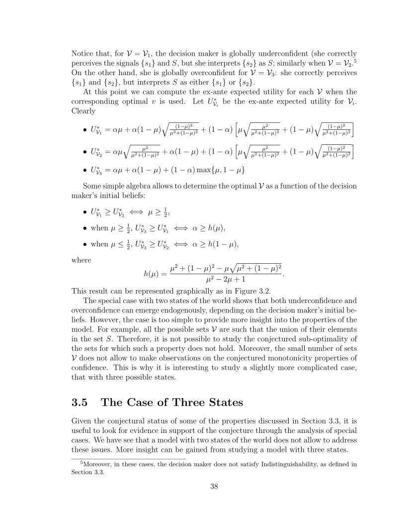
Notice that, for V = V1, the decision maker is globally underconfident (she correctlyperceives the signals s1 and S, but she interprets s2 as S; similarly when V = V2.5

On the other hand, she is globally overconfident for V = V3: she correctly perceivess1 and s2, but interprets S as either s1 or s2.

At this point we can compute the ex-ante expected utility for each V when thecorresponding optimal v is used. Let U∗Vi be the ex-ante expected utility for Vi.Clearly

• U∗V1= αµ+ α(1− µ)

√(1−µ)2

µ2+(1−µ)2 + (1− α)[µ√

µ2

µ2+(1−µ)2 + (1− µ)√

(1−µ)2

µ2+(1−µ)2

]• U∗V2

= αµ√

µ2

µ2+(1−µ)2 + α(1− µ) + (1− α)[µ√

µ2

µ2+(1−µ)2 + (1− µ)√

(1−µ)2

µ2+(1−µ)2

]• U∗V3

= αµ+ α(1− µ) + (1− α) maxµ, 1− µ

Some simple algebra allows to determine the optimal V as a function of the decisionmaker’s initial beliefs:

• U∗V1≥ U∗V2

⇐⇒ µ ≥ 12,

• when µ ≥ 12, U∗V3

≥ U∗V1⇐⇒ α ≥ h(µ),

• when µ ≤ 12, U∗V3

≥ U∗V2⇐⇒ α ≥ h(1− µ),

where

h(µ) =µ2 + (1− µ)2 − µ

√µ2 + (1− µ)2

µ2 − 2µ+ 1.

This result can be represented graphically as in Figure 3.2.The special case with two states of the world shows that both underconfidence and

overconfidence can emerge endogenously, depending on the decision maker’s initial be-liefs. However, the case is too simple to provide more insight into the properties of themodel. For example, all the possible sets V are such that the union of their elementsin the set S. Therefore, it is not possible to study the conjectured sub-optimality ofthe sets for which such a property does not hold. Moreover, the small number of setsV does not allow to make observations on the conjectured monotonicity properties ofconfidence. This is why it is interesting to study a slightly more complicated case,that with three possible states.

3.5 The Case of Three States

Given the conjectural status of some of the properties discussed in Section 3.3, it isuseful to look for evidence in support of the conjecture through the analysis of specialcases. We have see that a model with two states of the world does not allow to addressthese issues. More insight can be gained from studying a model with three states.

5Moreover, in these cases, the decision maker does not satisfy Indistinguishability, as defined inSection 3.3.

38

Figure 3.2: Under- and Overconfidence with Two States

Unfortunately, the analysis in this case is computationally much more complicatedthan in the model with two states. First, to describe initial beliefs six parametersare needed: µ(s1), µ(s2), p(s1), p(s2), p(s3), and p(sS).6 Moreover, |Σ| = 7,implying that different values of V must be considered (two, three, four, five, andsix).

To overcome this difficulties, I have used Matlab to solve the problem numerically.The main steps of the program are the following:

• fixing specific parameters values, the optimal act is computed for any possiblesignal observed (this step can be easily solved analytically);

• for any set V of observable signals and for any signal received, the program findsthe corresponding signal in V maximizing (ex-post) expected utility;

• it is then possible to compute, for each V , the corresponding ex-ante expectedutility; the program selects the set V for which utility is maximized.

In this way, the program finds the optimal V for a specific value of the decisionmaker’s initial beliefs. A more general problem is to determine whether a given Vcan be optimal for some values of the parameters. To do this, I have constructed a

6The remaining values can be derived as follows:µ(s3) = 1− µ(s1)− µ(s2),p(s1, s2) = 1−p(s1)−p(s2)+p(s3)−p(sS)

2 ,p(s1, s3) = 1−p(s1)+p(s2)−p(s3)−p(sS)

2 ,p(s2, s3) = 1+p(s1)−p(s2)−p(s3)−p(sS)

2 .

39

function that, after computing the optimal V , assigns the value 0 to the one underconsideration, and 1 to all the others. Minimizing this function over the possiblevalues of the parameters, it is possible to see whether that particular set V can everbe optimal: this is case when the minimum of the function is 0. A detailed descriptionof the program can be found in Appendix C.

Using this algorithm, I find the following results:

• only sets V such that⋃E : E ∈ V = S can be optimal for some initial beliefs;

• all the sets V satisfying this property are optimal for some values of the param-eters, except s1, s1, s2, s1, s3.

Appendix C gives example of initial beliefs that make each set V optimal. The resultssupport the conjectures in Section 3.3.

However, there is a caveat. The algorithm use for the maximization problem looksfor local maxima only. Although I used a grid of initial values for the six parameters,the possibility of having missed some optimal solutions cannot be excluded.

3.6 Conclusions

This chapter has introduces a model in which a decision maker is aware that shecannot extract all the information from the observation of events. She knows that thenumber of possible signals is larger than the number of different pieces of informationshe can handle. At an ex-ante stage, she therefore wants to optimally map ”true”signals into ”perceived” one, so that to maximize her ex-ante expected utility.

The analysis of optimal mapping performed in this chapter is clearly partial. Fewresults have been established, while the main properties are just presented as conjec-tures. Although intuitively simple, the model is mathematically quite complex. Ofcourse, better results can be obtained with a deeper analysis. In particular, Conjec-tures 3.3.1 and 3.3.2 are clearly provable (or disprovable).

What emerges, however, is the presence of very limited structure. An optimalmapping does not necessarily exhibit any kind of ”confidence monotonicity” or even”information monotonicity” (see Subsection 3.3.3). However, this does not excludethe possibility of the emergence of more structure once the set of possible initialbeliefs is reduced. I am thinking in particular to restriction on the values of thelikelihood functions p, which may be reasonable in particular contexts. Studyingwhether there exist relations between restrictions on p and structural properties ofthe optimal mapping may be an interesting area of future research.

40

Appendix A

Proofs for Chapter 1

A.1 Proof of Theorem 1.4.1

The following simple lemma has a crucial role in the proof.

Lemma A.1.1. Consider x, y ∈ (0, 1)n with x(n) 6= y(n) and αin−1i=1 , where αi > 0

and∑n−1

i=1 αi < 1. There exist scalars kini=0 such that

n−1∏i=1

xαii x1−Pαi

n Tn−1∏i=1

yαii y1−Pαi

n ⇐⇒ k0 +n−1∑i=1

kiαi T 0.

Proof. Simple algebra shows that the relation is satisfied for any (k0, ..., kn−1) suchthat

kik0

=lnxi − lnxn − ln yi + ln yn

lnxn − ln yn, i = 1, ..., n− 1.

What the lemma says is that, given a likelihood function (which is represented bythe vectors x and y), there exists a unique hyperplane separating the limit frequenciesfor which beliefs converge to (1, 0) and those for which beliefs converge to (0, 1).Therefore, any likelihood function can be associated with a hyperplane.

Consider the case µ ∈ ∆(L1,L2). Assume that there exist two limit frequenciesr1, r2 ∈ int∆(S) such that

rt → r1 ⇒ µt → δL1 ,

rt → r2 ⇒ µt → δL2 .

If this is not true, then there is nothing to prove.Consider any recursive updating rule satisfying the conditions of the theorem.

Suppose that µ = (1, 0) or µ = (0, 1) can be reached in finite time with positiveprobability; in what follows I consider the first case, but the argument clearly appliesto the other, too. There are two cases: either there exists s ∈ S such that f(s, (1, 0)) 6=(1, 0), or no such outcome exists. The second case can be easily dismissed. In fact,given any limit frequencies, the probability of observing the sequence of outcomes

41

leading to µ = (1, 0) is positive; but since there must exist limit frequencies withdifferent limit beliefs, we are led to a contradiction. In order to get rid of the first case,consider a limit frequency for which we expect convergence to µ = (1, 0). Clearly,as µ approaches (1, 0), the probability of reaching (1, 0) in finite time must go tozero. Otherwise, there would not be a t such that for all ε, δ > 0, prob(µt′ /∈ (1, 1 −ε)) < δ,∀t′ > t. Therefore, if the only thing we are interested in is convergence,we can disregard the possibility of reaching µ = (1, 0) in finite time: if an updatingmechanism exists for which µ converges to (1, 0), then convergence has to be possiblefor some mechanism in which (1, 0) is not reached in finite time. So, if we provethat no mechanism of this last type exists, we can conclude that the appropriateconvergence cannot be obtained with any recursive mechanism.

Once we exclude the previous cases, µt+1 can be obtained from µt multiplying eachcomponent µi by a positive scalar. Formally, there exists a function v : (S,∆(S))→R2

++ such that

f(s, µ) =

(v(s, µ)iµi∑i v(s, µ)iµi

)2

i=1

.

Moreover, we can always use the normalization∑

i v(s, µ)i = 1 (so that each f isassociated to a unique v).

The following lemma shows the consequences for the function v of assuming thatf is well-behaved. It turns out that v has a limit when beliefs approach certainty.Although it would be nice to get rid of this hypothesis, it’s still unclear whether thetheorem holds in the more general case.

Lemma A.1.2. If f is well-behaved, then v(., µ) converges to a limit function forµ→ (1, 0) and for µ→ (0, 1).

Proof. Convergence of v(., µ) means convergence of v(s, µ) for any s ∈ S. Let’sconsider a generic s. To simplify notation, I will drop the argument s in the proofof this lemma. Therefore, f(µ) and v(µ) must be interpreted as f(s, µ) and v(s, µ)respectively. In addition, I will redefine µ ∈ [0, 1] as the probability associated to L1.

Define z(µ) := v1(µ)v2(µ)

. Then we can write

f(µ) =z(µ)µ

z(µ)µ+ (1− µ)

or, equivalently,

z(µ) =

1−µµf(µ)

1− f(µ).

Let’s consider the case in which µ→ 1; to address the other case, just take the limitof z(µ)−1 as µ→ 1. Computing the limit, we get

limµ→1

z(µ) = limµ→1

1−µµf(µ)

1− f(µ)=

42

= limµ→1

f(µ)µ2 − f ′(µ)1−µ

µ

f ′(µ)= lim

µ→1f ′(µ)−1.

Since f is well-behaved, this limit exists (not necessarily finite).

By Lemma A.1.2, as µ→ (1, 0) or µ→ (0, 1), v(., µ) converges to a limit function.Both limits are, according to the definition in Section 3, likelihood functions. As wealready know, such functions can be associated to hyperplanes separating the half-spaces of limit frequencies for which µt converges to (1, 0) or (0, 1) if updating ischaracterized by the likelihood function itself. We now need to prove the followingresults:

• Consider a limit frequency such that beliefs converge to (1, 0). I claim thatthe same convergence result must hold if updating is performed using the limitlikelihood function for µ→ (1, 0).

• Consider any limit frequency belonging to the half-space where beliefs convergeto (1, 0) according to the limit likelihood function for µ→ (1, 0). Clearly, thereexists ε > 0 such that for any ε′ < ε, the limit frequency lays on the same”side” with respect to the hyperplanes associated to the functions v(., µ) forµ = (1 − ε′, ε′). I then claim that, for µ0 sufficiently close to (1, 0), beliefsconverge to (1, 0) with positive probability.

To prove the first point, suppose that the convergence result does not hold forthe limit likelihood function. Then, since beliefs converge to (1, 0), there must be at such that, for any t′ > t, beliefs are updated using likelihood functions that, eachby themselves, would lead to convergence to (0, 1).1 I want to show that this is notpossible. The following lemma provides this result.

Lemma A.1.3. Consider a sequence of likelihood functions gt∞t=1 and suppose up-dating is performed at each period t using the likelihood function gt. Let p ∈ ∆(S) bea limit frequency such that, for any t, beliefs µn converge to (0, 1) ((1, 0)) for n→∞when updating is performed using the likelihood function gt in every period. Then,when we use, at each period t, the likelihood function gt, beliefs converge to (0, 1)((1, 0)).

Proof. Let i(st) : Ω → 1, ..., S be the random variable whose value is the indexof the observation at time t; that is, i(st) says which element of S is observed inperiod t. Since the experiments are not identical nor independent, i(st) depends onthe history (s1, ..., st−1). Let (xi,t, yi,t)

Si=1 : S → R2

++ be the likelihood function inperiod t. The decision maker does not remember past observations; therefore, thelikelihood function can only depend on µt−1. Studying beliefs convergence means tolook at the limit of

n∏t=1

((yi(st),txi(st),t

) ∣∣∣∣(s1, ..., st−1),t−1∏h=0

(yi(sh),h

xi(sh),h

)µ0

),

1I am implicitly excluding the case in which the limit frequency belongs to the hyperplane cor-responding to the limit likelihood function. This can be safely done since the theorem deals withlimit frequencies in open sets.

43

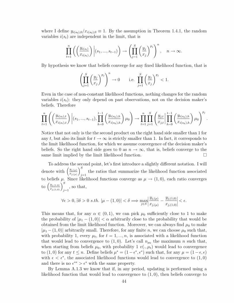
where I define yi(s0),0/xi(s0),0 ≡ 1. By the assumption in Theorem 1.4.1, the randomvariables i(st) are independent in the limit, that is

n∏t=1

((yi(st)xi(st)

) ∣∣∣∣(s1, ..., st−1)

)→

(S∏j=1

(yjxj

)pj)n

, n→∞.

By hypothesis we know that beliefs converge for any fixed likelihood function, that is(S∏j=1

(yjxj

)pj)n

→ 0 i.e.S∏j=1

(yjxj

)pj< 1.

Even in the case of non-constant likelihood functions, nothing changes for the randomvariables i(st): they only depend on past observations, not on the decision maker’sbeliefs. Therefore

n∏t=1

((yi(st),txi(st),t

) ∣∣∣∣(s1, ..., st−1),t−1∏h=0

(yi(sh),h

xi(sh),h

)µ0

)→

n∏t=1

S∏j=1

(yj,txj,t

∣∣∣∣ t−1∏h=0

(yi(sh),h

xi(sh),h

)µ0

)pj

.

Notice that not only is the the second product on the right hand side smaller than 1 forany t, but also its limit for t→∞ is strictly smaller than 1. In fact, it corresponds tothe limit likelihood function, for which we assume convergence of the decision maker’sbeliefs. So the right hand side goes to 0 as n → ∞, that is, beliefs converge to thesame limit implied by the limit likelihood function.

To address the second point, let’s first introduce a slightly different notation. I will

denote with(yj,(µ)

xj,(µ)

)Sj=1

the ratios that summarize the likelihood function associated

to beliefs µ. Since likelihood functions converge as µ → (1, 0), each ratio converges

to(yj,(1,0)

xj,(1,0)

)Sj=1

, so that,

∀ε > 0,∃δ > 0 s.th. |µ− (1, 0)| < δ =⇒ maxj∈S

yj,(µ)

xj,(µ)

−yj,(1,0)

xj,(1,0)

< ε.

This means that, for any α ∈ (0, 1), we can pick µ0 sufficiently close to 1 to makethe probability of |µ1 − (1, 0)| < α arbitrarily close to the probability that would beobtained from the limit likelihood function. Moreover, we can always find µ0 to make|µ1− (1, 0)| arbitrarily small. Therefore, for any finite n, we can choose µ0 such that,with probability 1, every µt, for t = 1, ..., n, is associated with a likelihood functionthat would lead to convergence to (1, 0). Let’s call nµ0 the maximum n such that,when starting from beliefs µ0, with probability 1 v(., µt) would lead to convergenceto (1, 0) for any t ≤ n. Define beliefs µ∗ = (1− ε∗, ε∗) such that, for any µ = (1− ε, ε)with ε < ε∗, the associated likelihood functions would lead to convergence to (1, 0)and there is no ε∗∗ > ε∗ with the same property.

By Lemma A.1.3 we know that if, in any period, updating is performed using alikelihood function that would lead to convergence to (1, 0), then beliefs converge to

44

(1, 0). Therefore, for any µ0, µ and p ∈ (0, 1), there exists a smallest Nµ0,µ,p suchthat, with probability p, µt > µ for any t > Nµ0,µ,p.

2

Now fix µ = µ∗. If we can prove that, for some µ0 > µ∗ and some p, nµ0 > Nµ0,µ∗,p,then the proof of the second point is completed. But nµ0 can be taken arbitrarily largeif we choose µ0 sufficiently close to (1, 0), while limµ0→(1,0)Nµ0,µ∗,p is clearly bounded.

From the two points above, it follows that, in order to have convergence to thetrue parameter whenever the limit frequency falls in int(L1 \ L2) or int(L2 \ L1), anecessary condition is the existence of a hyperplane separating the two sets. However,if S > 3, this may not be the case, as is clear from the example described by FigureA.1, where S = 4.

Figure A.1: Three-dimensional Sets

Whatever hyperplane we choose, there will be frequencies in int(L1\L2) for whichbeliefs converge to δL2 and/or frequencies in int(L2 \ L1) for which beliefs convergeto δL1 . This completes the proof.

A.2 Proof of Theorem 1.4.2

Lemma A.2.1. Let A,B ⊂ R2 be two closed and convex sets such that B = A+ k =x + k ∈ R2 : x ∈ A for some k ∈ R2. There exist disjoint convex sets A′ and B′

with A \B ⊂ A′ and B \ A ⊂ B′.

Proof. Suppose there exist x ∈ A ∩ B, y1, y2 ∈ A \ B, z1, z2 ∈ B \ A, β, γ ∈ (0, 1)such that x = βy1 + (1− β)y2 = γz1 + (1− γ)z2. By construction, y1 + k, y2 + k ∈ Band z1− k, z2− k ∈ A. Since A and B are convex, co(y1, y2, z1− k, z2− k) ⊂ A andco(z1, z2, y1 + k, y2 + k) ⊂ B. Notice that these two sets are convex quadrangles,they have nonempty intersection (they both contain x) and one is the translation ofthe other. It is easy to verify that these conditions imply that, for some i ∈ (1, 2),either yi ∈ B or zi ∈ A. But this is a contradiction. Therefore no x ∈ A∩B can be a

2Since the set S is finite, µt(.) ∝ v(., µt−1)µt−1 converges in probability if and only if it convergesalmost surely.

45

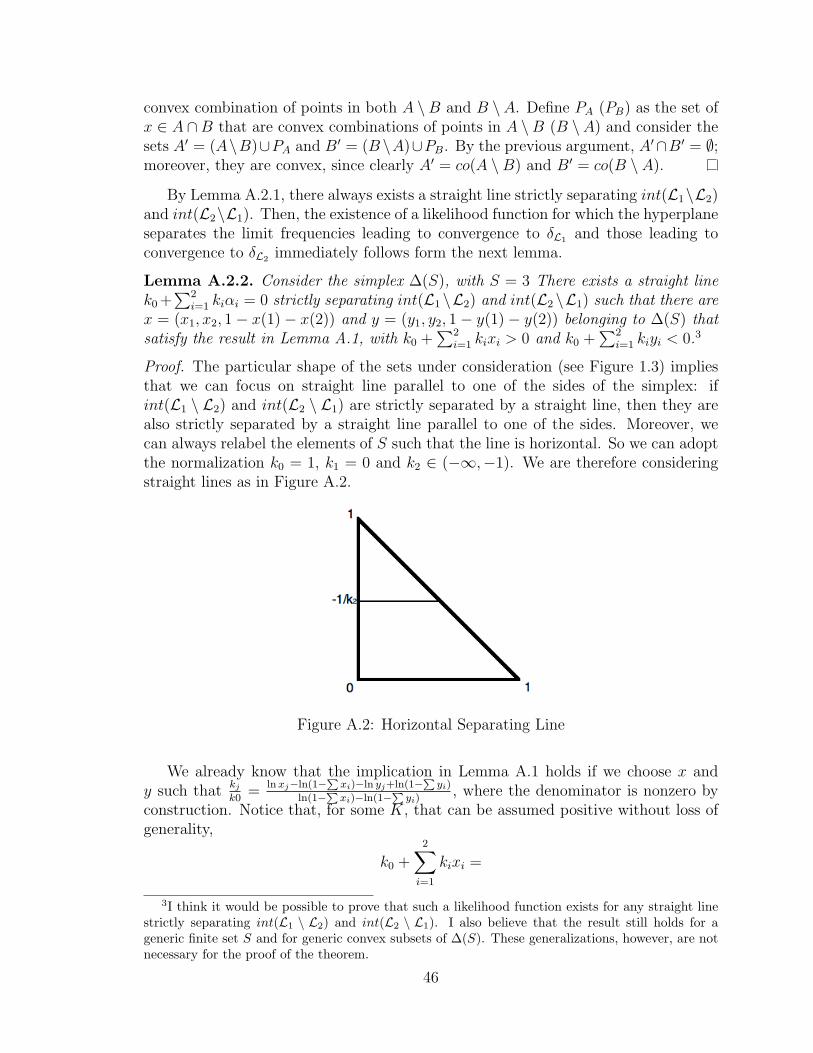
convex combination of points in both A \B and B \A. Define PA (PB) as the set ofx ∈ A ∩B that are convex combinations of points in A \B (B \A) and consider thesets A′ = (A\B)∪PA and B′ = (B \A)∪PB. By the previous argument, A′∩B′ = ∅;moreover, they are convex, since clearly A′ = co(A \B) and B′ = co(B \ A).

By Lemma A.2.1, there always exists a straight line strictly separating int(L1\L2)and int(L2\L1). Then, the existence of a likelihood function for which the hyperplaneseparates the limit frequencies leading to convergence to δL1 and those leading toconvergence to δL2 immediately follows form the next lemma.

Lemma A.2.2. Consider the simplex ∆(S), with S = 3 There exists a straight linek0 +

∑2i=1 kiαi = 0 strictly separating int(L1 \L2) and int(L2 \L1) such that there are

x = (x1, x2, 1− x(1)− x(2)) and y = (y1, y2, 1− y(1)− y(2)) belonging to ∆(S) thatsatisfy the result in Lemma A.1, with k0 +

∑2i=1 kixi > 0 and k0 +

∑2i=1 kiyi < 0.3

Proof. The particular shape of the sets under consideration (see Figure 1.3) impliesthat we can focus on straight line parallel to one of the sides of the simplex: ifint(L1 \ L2) and int(L2 \ L1) are strictly separated by a straight line, then they arealso strictly separated by a straight line parallel to one of the sides. Moreover, wecan always relabel the elements of S such that the line is horizontal. So we can adoptthe normalization k0 = 1, k1 = 0 and k2 ∈ (−∞,−1). We are therefore consideringstraight lines as in Figure A.2.

Figure A.2: Horizontal Separating Line

We already know that the implication in Lemma A.1 holds if we choose x andy such that

kjk0

=lnxj−ln(1−

Pxi)−ln yj+ln(1−

Pyi)

ln(1−Pxi)−ln(1−

Pyi)

, where the denominator is nonzero byconstruction. Notice that, for some K, that can be assumed positive without loss ofgenerality,

k0 +2∑i=1

kixi =

3I think it would be possible to prove that such a likelihood function exists for any straight linestrictly separating int(L1 \ L2) and int(L2 \ L1). I also believe that the result still holds for ageneric finite set S and for generic convex subsets of ∆(S). These generalizations, however, are notnecessary for the proof of the theorem.

46

= K[ln(1−∑

xi)−ln(1−∑

yi)]+∑

K[lnxi−ln(1−∑

xj)−ln yi+ln(1−∑

yj)]xi =

= K[ln(1−∑

xi)− ln(1−∑

yi)](1−∑

xi) +∑

(lnxi − ln yi)xi > 0.

where the inequality is immediate, provided x 6= y. Similarly, k0 +∑S−1

i=1 kiyi < 0.We still need to prove that we can find x and y that satisfy the equalities above andbelong to ∆(S). Simple algebra provides the functional relation between x and y. Infact,

yj

(1−∑yi)

“1+

kjk0

” =xj

(1−∑xi)

“1+

kjk0

” , j = 1, 2, (A.1)

where by construction∑yi 6=

∑xi.

Consider x ∈ int(∆(S)) and assume we are able to find y satisfying equations(A.1) and such that y1 > 0. Then, taking the equation for i = 1, it must be thecase that 1 − y1 − y2 > 0; this in turn implies, from the equation with i = 2, thaty2 > 0, that is, y ∈ int(∆(S)). Also notice that x 6= y implies x1 6= y1. So we simplyhave to show that for any straight line, that is for any k2 ∈ (−∞,−1), there existsx ∈ int(∆(S)) such that there is y satisfying the equations above, with y1 > 0 andy1 6= x1.

Let’s take x2 = − 1k2

+ ε, for ε > 0. From the system of equations above we get

(1 + k2(1− ε))y−k21 − k2x1y

−k2−11 − (1− k2ε)x

−k21 = 0.

Since we want x2 < 1, clearly 1 + k2(1 − ε) < 0, while 1 − k2ε > 0. To simplifynotation, denote the first term as a and the second as b. It is also immediate to seethat any solution must have the form y1 = hx1, for some h > 0. Therefore all weneed is to find positive solutions to the equation

ah−k2 − k2h−k2−1 − b = 0.

First of all, notice that h = 1 is always a solution, and it is the only solution if ε = 0.For ε > 0, we want to prove that there exists another solution. The task is nontrivialsince k2 can be any real number in (−∞,−1). I will prove the result for k2 rational.Given the smooth nature of the equation, the result generalizes to the entire intervalby a continuity argument. Denote −k2 = α

β, where α, β ∈ N++ and α > β. With an

obvious change of variables, we obtain the equation

azα +α

βzα−β − b = 0.

I am going to use Sturm’s theorem (see, for example, [16]) to show that such anequation always has two and only two positive solutions. First we have to constructa particular sequence of polynomials called Sturm chain. The first element is thepolynomial azα + α

βzα−β − b itself; the second is its derivative. Every other element

is computed as the reminder of the polynomial division between the two polynomialsimmediately above, with its sign changed. Notice that the degree of the polynomialsin the chain is strictly decreasing. The chain ends when the last polynomial has

47

degree 1. To find the number of distinct positive real roots of our equation, we haveto determine the signs of each polynomial in the chain corresponding to z = 0 andz → +∞ and to see how many times signs flip in these two cases. Sturm’s theoremstates that the number of solutions is equal to the difference between the numbers ofsign flips for z = 0 and z → +∞.

In order to find the number of solutions, it is not really necessary to computethe Sturm chain. All we need are the corresponding sequences of the exponentsappearing in the polynomials and the signs of the coefficients. I am now going toshow how these sequences can be computed. For the moment, I will build genericsequences, disregarding the specific values of α and β for which some exponent turnsout to be 0. I will show later how to handle these cases. So in what follows, anyexponent that is not explicitly 0 is assumed to be positive. On the other hand, I willindicate as special cases the values of α and β that change the functional form of theexponents with respect to the general case. How the chain evolves after these specialcases will be examined later.

The first three elements of the sequences are easy to compute.

ElementGeneral case Special cases

Exponents Coefficients’ signs Exponents Coefficients’ signs

1 α, α− β, 1 - + -

2 α− 1, α− β − 1 - +

3 α− β, 0 - +β = 1

α− 2, 0 - +

From this point on, signs and exponents can be computed following simple rules,whose proof is straightforward and omitted. If the element number is even, the sign ofthe first term is the opposite to that of the second term of the one to the last element;the sign of the second term is the product of the signs of the terms of the last elementtimes the sign of the first term of the one to the last element. For elements whosenumber is odd, the rules for determining the signs of the two terms are switched. Therule for the exponents follows a cyclical scheme, shown in the table below.

Element General case Special cases

2 g1, g2

3 g2 + 1, 0g1 = g2 + 1

g2, 0

4g2, g3 g2 = g3

(depending on the relation between g1 and g2) g2

5 g3 + 1, 0g2 = g3 + 1

g3, 0

6g3, g4 g3 = g4

(depending on the relation between g2 and g3) g3

48

The cyclicality of the exponents is apparent; the specific form of the second ex-ponent in the even elements is not important for the result. Knowing these rules, wecan easily find the actual sequences.4

El.General case Special cases

Exponents Signs Exponents Signs

4α− β − 1,

- +α = i

i−1β

(i− 1)β − (i− 2)α− 1for α ∈

[ii−1β, i−1

i−2β)

α− β − 1 -

5 (i− 1)β − (i− 2)α, 0 + -α = i

i−1β + 1

i−1

(i− 1)β − (i− 2)α− 1, 0 + -

6(i− 1)β − (i− 2)α− 1,

- +α = (j+2)i−(j+1)

(j+2)i−(3+2j)β

[(i− 2)j + (i− 1)]α− [(i− 1)j + i]β − 1

for α ∈(

(j+1)i−j(j+1)i−(1+2j)

β, (j+2)i−(j+1)(j+2)i−(3+2j)

β]

(i− 1)β − (i− 2)α− 1 +

7 [(i− 2)j + (i− 1)]α− [(i− 1)j + i]β, 0 + -α = (j+2)i−(j+1)

(j+2)i−(3+2j)β + 1

(j+2)i−(3+2j)

[(i− 2)j + (i− 1)]α+ + -−[(i− 1)j + i]β − 1, 0

Notice the cyclicality of the sequence of the signs: the signs at elements 6 and7 are the same as at elements 2 and 3. The same cyclicality (with cycles of length4 starting from element 4) is therefore inherited by the sequence of the signs of thepolynomials for z = 0 and z →= ∞ and, in turn, by the sequence of the differencebetween the numbers of sign flips.

Element 1 2 3 4 5 6 70 - 0 + 0 - 0 +

+∞ - - - - + - -Difference 0 0 1 1 1 0 1

We now have to consider all the cases in which the sequence ends. It is easy tosee that this can happen only when:

• we are in one of the special cases considered above; we will see that in thesecases the sequence ends after at most two additional steps;

• the second term of an even element has exponent 0; the sequence ends after twoadditional steps;

• an even element has degree 0.

4The signs for the special cases of elements 4 and 6 are more difficult to compute. However, wewill see that there is a shortcut to get the results.

49

For each of these cases, we need to check whether the difference between the numbersof sign flips turns out to be 2. Let’s look at the table with the rule for computingthe exponents and let’s start with the cases of the type g2 = g3 (g2 > 0) in an evenelement of the sequence. In this case, in the next step, the power of the polynomialis 0 and the sequence ends. Obviously, the signs for z = 0 and z → +∞ must be thesame. So we have a situation like

Element Even Odd0 0 s2

+∞ s1 s2

To determine the values of s1 and s2, notice that at any odd element the sign forz = 0 is the opposite than that for z → +∞, and the difference between signs flipsis 1. Moreover, we know that at least one positive solution exists, that is z = 1. Theonly way the final difference between sign flips can be at least one is that s1 be thesame as the corresponding sign for the element immediately above and s2 = s1. Butin this case the number of sign flips turns out to be 2.

Let’s consider now the cases of the sort g2 = g3 + 1, which are special for oddelements. It is easy verifiable that we can only have the following sub-cases:

• if g2 > 2, the next element has coefficients (1, 0) and the same signs as theelement immediately above, so that the difference between sign flips is still 1;the sequence ends after another step, where, again by the fact that a solutionexists, the sign must be the opposite of the first sign of the last step; this impliesthe existence of two solutions;

• if g2 = 2, the sequence ends at the next step; the existence of two solutionsfollows by the same argument.

When the second term of an even element has exponent 0, the following holds:

• the sign for z = 0 becomes +; notice that this implies that the difference betweensign flips is 1;

• the next element has exponents (1, 0) and the signs are still computed accordingto the general rule; this does not change the difference;

• the usual argument determines the sign at the final step, proving the existenceof two solutions.

It remains to analyze the cases in which an even element has degree 0. Again, theusual argument gives the sign and implies the existence of two solutions.

This completes the proof of Theorem 1.4.2 for the case S = 3. It can be easilyadapted to the case S = 2.

50

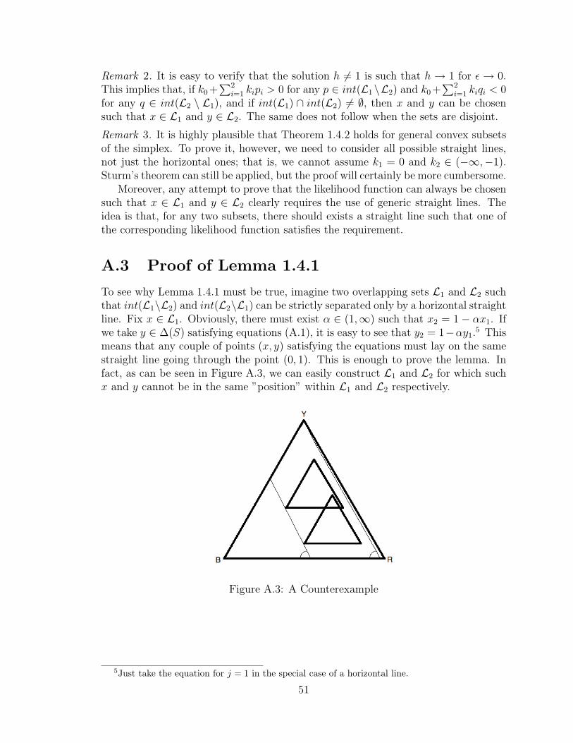
Remark 2. It is easy to verify that the solution h 6= 1 is such that h → 1 for ε → 0.This implies that, if k0 +

∑2i=1 kipi > 0 for any p ∈ int(L1\L2) and k0 +

∑2i=1 kiqi < 0

for any q ∈ int(L2 \ L1), and if int(L1) ∩ int(L2) 6= ∅, then x and y can be chosensuch that x ∈ L1 and y ∈ L2. The same does not follow when the sets are disjoint.

Remark 3. It is highly plausible that Theorem 1.4.2 holds for general convex subsetsof the simplex. To prove it, however, we need to consider all possible straight lines,not just the horizontal ones; that is, we cannot assume k1 = 0 and k2 ∈ (−∞,−1).Sturm’s theorem can still be applied, but the proof will certainly be more cumbersome.

Moreover, any attempt to prove that the likelihood function can always be chosensuch that x ∈ L1 and y ∈ L2 clearly requires the use of generic straight lines. Theidea is that, for any two subsets, there should exists a straight line such that one ofthe corresponding likelihood function satisfies the requirement.

A.3 Proof of Lemma 1.4.1

To see why Lemma 1.4.1 must be true, imagine two overlapping sets L1 and L2 suchthat int(L1\L2) and int(L2\L1) can be strictly separated only by a horizontal straightline. Fix x ∈ L1. Obviously, there must exist α ∈ (1,∞) such that x2 = 1− αx1. Ifwe take y ∈ ∆(S) satisfying equations (A.1), it is easy to see that y2 = 1−αy1.5 Thismeans that any couple of points (x, y) satisfying the equations must lay on the samestraight line going through the point (0, 1). This is enough to prove the lemma. Infact, as can be seen in Figure A.3, we can easily construct L1 and L2 for which suchx and y cannot be in the same ”position” within L1 and L2 respectively.

Figure A.3: A Counterexample

5Just take the equation for j = 1 in the special case of a horizontal line.

51

Appendix B

Proofs for Chapter 2

B.1 Proof of Proposition 2.3.1

Let’s prove that the representation implies the axiom. First, ∀E ∈ Σ, E ⊆ v(E),as required by Axiom 4. Now, consider s /∈ E that is also %E-null, and supposethat there exists s′ ∈ E such that s and s′ are indistinguishable. I will denoteindistinguishability with the notation %s=%s

′. Since E ⊆ V E, we have s′ ∈ V E.Similarly, s ∈ V s and s′ ∈ V s′. Since %s=%s

′, V s = V s′, so that s ∈ V s′.

Since V is closed under intersections, (V s′∩V E) ∈ V . We know that s′ ∈ (V s

′∩V E),but (V s

′ ∩ V E) ⊂ V s′ , because s /∈ V E. This contradicts point (iii).We need now to show that, if there exists s /∈ E that is also %E-non-null, there

must exist an indistinguishable s′ ∈ E. Before doing this, let’s prove a preliminaryresult. Given two states s1 and s2, either V s1 = V s2 or the two are disjoint.Suppose V s1 ∩ V s2 6= ∅ and consider the following two cases:

• s1 /∈ V s2. Since V is an algebra, V s1 \ (V s1 ∩ V s2) ∈ V . Moreover,s1 ∈ V s1 \ (V s1 ∩ V s2) ⊂ V s1. This contradicts point (iii). The argumentis the same is we invert s1 and s2.

• s1 ∈ V s2 and s2 ∈ V s1. Since s1 ∈ (V s1 ∩ V s2), point (iii) implies thatV s1 ⊆ V s2. Similarly, we must have V s2 ⊆ V s1 and so V s1 = V s2.

Now, let s /∈ E be %E-non-null and suppose that, for any s′ ∈ E, %s=%s′. The

representation requires that V s 6= V s′. We have already shown that this implies

that V s ∩ V s′ = ∅. So, for any s′ ∈ E, s′ is %s-null. Therefore E is %s-null;that is, E ∩ V s = ∅. Clearly, S ∈ V and, since V is an algebra, S \ V s ∈ V . BeingE ⊆ S \ V s, point (iii) implies that V E ⊆ S \ V s. Since s ∈ V s, we have that sis %E-null, which contradicts the hypothesis.

It remains to be proved that the axiom implies the representation. Points (i) and(ii) are the same as in Proposition 2.2.1. So I am going to show that Axiom 4 impliesboth Axioms 2 and 3. Axiom 3 obviously holds: given a signal E any s ∈ E is %E-non-null. Suppose Axiom 2 is not satisfied. Then, for some signal E, v(v(E)) 6= v(E).By Axiom 4, v(E) ⊆ v(v(E)). Given s ∈ v(v(E)) \ v(E), there exists s′ ∈ v(E) suchthat %s=%s

′. But there also exists s′′ ∈ E such that %s′=%s

′′ (this may even

52

be s′ itself). Therefore s is indistinguishable from some state in E, and Axiom 4implies that s ∈ v(E), which contradicts the hypothesis.

For point (iii), we already know that E ⊆ v(E). Suppose now that there exists asignal F which is a fixed point of v and such that E ⊆ F ⊂ v(E). Since v(F ) = F , byAxiom 4 there is no s ∈ v(E) \ F such that s is indistinguishable from some state inF . Given that E ⊆ F , again by Axiom 4 s cannot be contained in v(E), contradictingthe hypothesis.

The last thing to prove is that the fixed points of v constitute an algebra. LetE and F be two fixed points of v. Then there is no s /∈ E that is indistinguishablefrom a state in E, and similarly there is no s′ /∈ F that is indistinguishable fromsome state in F . Therefore, no state in (E ∩ F )c can be indistinguishable from somestate in E ∩ F . So v(E ∩ F ) = E ∩ F and the set of fixed points of v is closed underintersections. Closure under complements is obvious.

B.2 Proof of Proposition 2.4.1

Let’s first prove that the representation implies the axioms. Axioms 2 and 3 areobviously implied. To prove Axiom 6, let s ∈ V A \ A and suppose that there is nos′ ∈ A such that %s

′=%s, that is, such that V s′ = V s. Properties (iv)1 and

(iv)3 and the closure of V under intersection imply that V s is the smallest elementof V that contains s. In fact, by (iv)1, V s must contain s; it cannot be a superset ofsome other element of V containing s, because of (iv)3. And there cannot be multiplesets satisfying these properties, because their intersection would still belong to V ,leading to a contradiction. It is therefore obvious that, if V s = V s

′, then both sand s′ are in V s. But I need the inverse result: I want to show that, if V s 6= V s

′,then s′ /∈ V s. Suppose that this is not true, that is, s′ ∈ V s and consider thefollowing two cases:

• we cannot have V s ⊂ V s′, because V s

′ is the smallest element of V con-taining s′;

• if V s \ V s′ 6= ∅, (iii) implies that V s \ V s′ ∈ V . Since V s \ V s′ ⊂ V s,it cannot include the state s. Therefore s ∈ V s′. By (iii), V s ∩ V s′ ∈ V .Clearly, s ∈ V s ∩ V s′ and V s ∩ V s′ ⊂ V s. But such a set cannot exist.

So we have proved that, for any s′ ∈ A, s′ /∈ V s. But V A \V s ∈ V , violating (iv)3.Axiom 7 is easily proved. Consider two indistinguishable states s and s′ such that

s ∈ V A, but s′ /∈ V A. it has already been proved that s, s′ ∈ V s. So V s ∩ V A ⊂V s. By (iii), V s ∩ V A ∈ V . This contradicts the fact that V s is the smallestelement of V containing s, as shown above.

Now I want to show that the axioms imply the representation. Properties (i) and(ii) immediately follow from Proposition 2.2.1. Let’s now prove that any signal A is%A-non-null (property (iv)1). Suppose not, so that A ∩ V = ∅. By Axiom 6, for anystate in V there exists an indistinguishable state in A. But Axiom 7 requires thatthe last state is conditionally non-null, which contradicts the initial hypothesis.

To prove that the set of fixed points of v is a semialgebra, we need to show that

53

• ∀A,B ∈ V , A ∩B ∈ V ;

• ∀A ∈ V , there exists a partition of S \ A whose elements belong to V .

Let’s first prove closure under intersections. Consider A,B ∈ V such that A ∩B 6= ∅. Since by assumption v(A) = A, Axiom 7 implies that no state in Ac isindistinguishable from some state in A. The same is true for B. Therefore, by Axiom6, v(A∩B) ⊆ A∩B. Suppose now that there exists s ∈ A∩B such that s /∈ v(A∩B).By Axiom 5, s must be %A-null, that is s /∈ v(A), but this is impossible. So A∩B ∈ V .

Before moving to the second part, it is useful to prove the other property of V ,that is, closure with respect to set difference. Take A,B ∈ V and suppose there existss such that s ∈ v(A \ B) and s /∈ A \ B. By Axiom 6, there exists s′ ∈ A \ Bwith %s

′=%s. Since by assumption v(A) = A, Axiom 7 implies that s ∈ A. Byassumption, s /∈ A ∩ B. On the other hand, since A ∩ B ∈ V , using Axioms 6 and 7we can immediately show that no state in A \B is indistinguishable from some statein A∩B, and therefore v(A \B)∩ (A∩B) = ∅. We have reached a contradiction, sowe can conclude that v(A \B) ⊆ A \B.

To prove the other direction, let’s first show that, for any A,B ∈ Σ, v(A ∪ B) ⊆v(A) ∪ v(B).1 Take s /∈ v(A) ∪ v(B) and consider two exhaustive cases.

1. s ∈ A or s ∈ B. Then by Axiom 5 s /∈ v(A ∪B).

2. s /∈ A ∪ B. We can consider two sub-cases. If there is no z ∈ A ∪ B such that%s=%z, then Axiom 6 implies that s /∈ v(A∪B). On the other hand, if sucha z exists, by Axiom 7 it must be the case that z /∈ A ∪B. Notice that Axiom7 also implies that s ∈ v(A∪B) if and only if z ∈ v(A∪B). But z falls in case1 above.

Take now A,B ∈ V . By the previous result, we have v(A) ⊆ v(A \B)∪ v(A∩B).By assumption, v(A) = A; moreover, v(A ∩ B) = A ∩ B, because V is closed underintersection. So, A \B ⊆ v(A \B).

To complete the proof of property (iii), let A ∈ V . We need to show that, for anys ∈ Ac, there exists an element of V that contains s and is disjoint from A. Closureunder intersection then provides the result. It is easy to see that the following twoproperties are sufficient for the proof:

• s ∈ V s;

• ∀A,B ∈ V , A \B ∈ V .

But the first result is a special case of (iv)1, which we have already proved, while thesecond is exactly what has been shown above.

Suppose now that property (iv)2 is not satisfied. So there exists V ∈ V such thatA ∩ V A ⊂ A ∩ V . Take s ∈ A ∩ (V \ V A) and consider the following two cases:

• suppose V A ⊂ V ; then Axiom 5(i) requires that v(V A ∪ s) = V A; but V A ∪s ⊆ V , so Axiom 5(ii) implies that s /∈ v(V ) = V , which contradicts theassumption;

1For an interpretation of this property see Section 2.5.

54

• if there exists s′ ∈ V A \ V , then by Axiom 6 there is a state s′′ ∈ A ∩ V A

such that s′ and s′′ are indistinguishable; since s′′ ∈ V and v(V ) = V , Axiom 7implies s′ ∈ V , which is false.

Proving property (iv)3 is easy. Take s ∈ V A \A. By Axioms 6 and 7, there existsa state s′ ∈ A ∩ V A indistinguishable from s. But A ∩ V A = A ∩ V ⊆ V = v(V ), sothat Axiom 7 implies s ∈ V .

Remark 4. Unlike in Proposition 2.3.1, Axiom 2 cannot be deduced from the oth-ers.On one hand, it is possible to exclude the existence of some E ∈ Σ such that∃s ∈ v(v(E)) \ v(E). In fact, Axiom 6 would imply that there exists s′ ∈ v(E) suchthat %s

′=%s. The state s′ is %E-non-null. Therefore, by Axiom 7, s must be%E-non-null, too, leading to a contradiction. On the other hand, the axioms are notsufficient to exclude the existence of some E ∈ Σ such that ∃s ∈ v(E) \ v(v(E)).

B.3 Proof of Corollary 2.4.1

We need to show that, for any V ∈ V and for any s ∈ V , there exists A ∈ Σ suchthat s ∈ A, A ⊆ V , v(A) = V , and, for any B with v(B) = V , B 6⊂ A. The proofcan be divided in three parts:

1. for any A with v(A) = V , A ∩ V 6= ∅;

2. let A be a signal such that s ∈ A and v(A) = V ; then there exists A′ ∈ A ∩ Vsuch that v(A′) = V ;

3. take any s ∈ V and let A be any subset of V such that s ∈ A and v(A) = V ;suppose there is a B ⊂ A such that s /∈ B and v(B) = V ; then there existsA′ ⊂ A such that s ∈ A′, v(A′) = V , and B 6⊂ A′.

It is straightforward to see how these three results establish the result. Part 1 isproperty (iv)1 in Proposition 2.4.1. Before moving to part 2, we need a preliminaryresult. I will prove that, for any signal A, v(A ∩ V A) = V A. If V A ⊂ A, then thereis nothing to prove: v(V A) = V A by Axiom 2. Suppose now that V A \ A 6= ∅. Forany s ∈ V A \ A, Axiom 6 requires the existence of s′ ∈ A such that %s

′=%s.On the other hand, since v(V A) = V A, Axiom 7 implies that no state in (V A)c isindistinguishable from some state in V A. Therefore, the s′ above must belong toA∩V A. Consider now the signal A∩V A. I claim that A∩V A ⊆ v(A∩V A). Supposenot; that is, suppose there exists z ∈ A ∩ V A such that z /∈ v(A ∩ V A). By Axiom5(ii), z must also be %A-null. But this is false. So we have proved that any state inV A \A is indistinguishable from some state in A∩V A and that any state in A∩V A is%A∩V A-non-null. Axiom 7 then implies that V A ⊆ v(A∩V A). By Axiom 6, any statein v(A∩V A)\ (A∩V A) must be indistinguishable from some state in A∩V A. But wehave already proved that no state in (V A)c can satisfy this requirement. Therefore,v(A ∩ V A) = V A. So part 2 is satisfied taking A′ = A ∩ V .

Part 3 is easily proved. Given that B ⊂ v(B), Axioms 6 and 7 imply that v(B)(that is to say V ) is the set of all the states that are indistinguishable from some

55

state in B. In particular, since s ∈ v(B), there must be a state s′ ∈ B such that%s

′=%s. Now take the signal A′ = (B \ s′) ∪ s. The set of indistinguishablestates must obviously be the same as for B, that is, the set V . If we can prove thatA′ ⊂ v(A′), then Axioms 6 and 7 imply that v(A′) = V . But this is immediatelyimplied by Axiom 5: any state in A′ \ v(A) should also be %V -null, and this is clearlyimpossible.

B.4 Proof of Proposition 2.5.1

Information monotonicity an be restated as an assumption on the monotonicity of thefunction v: if A ⊂ B, then v(A) ⊆ v(B). It is straightforward to see that Informationmonotonicity implies (iii). If not, then we could have A ∈ Σ and V ∈ V such thatA ⊆ V ⊂ v(A); since v(V ) = V , we have a contradiction. The other direction isequally trivial. Without Information monotonicity, there exist A,B ∈ Σ such thatA ⊂ B and v(B) ⊂ v(A). By global underconfidence we then have A ⊂ v(B) ⊂ v(A).Since v(B) ∈ V , we get a contradiction.

Consider now V1, V2 ∈ V . By Information monotonicity v(V1 ∩ V2) ⊆ v(V1) = V1

and v(V1 ∩ V2) ⊆ v(V2) = V2, that is v(V1 ∩ V2) ⊆ (V1 ∩ V2). Underconfidence thenimplies v(V1 ∩ V2) = (V1 ∩ V2), meaning that (V1 ∩ V2) ∈ V .

B.5 Proof of Proposition 2.5.2

The first part is obvious. To prove (i), consider V1, V2 ∈ V . Axiom 9 requires thatv(V1 ∪V2) ⊆ (V1 ∪V2). Underconfidence then implies v(V1 ∪V2) = (V1 ∪V2), meaningthat (V1 ∪ V2) ∈ V .

For (ii) we just need to prove that, for all signals A and B, v(A,B) ⊆ (v(A) ∪v(B)). By Proposition 2.5.1, we know that V ∪ ∅ is an algebra. By Axiom 8, forany A and B, v(A) and v(B) are the smallest elements of V such that A ⊆ v(A) andB ⊆ v(B). Therefore, (A ∪ B) ⊆ (v(A) ∪ v(B)) and, since (v(A) ∪ v(B)) ∈ V , itfollows from from Axiom 8 that v(A,B) ⊆ (v(A) ∪ v(B)).

56

Appendix C

Matlab Code and NumericalExamples for Chapter 3

C.1 Matlab Code

This section describes the Matlab code I used to study the model in the case ofthree states of the world. I also assumed u(x) =

√x. First, I want to compute the

optimal function v for specific values of the decision maker’s initial beliefs, given aconstraint on the number of observable signals. In the code, I use k to devote V andthe following intuitive notation for the initial beliefs: mu 1 = µ(s1), mu 2 = µ(s1),p 1 = p(s1), p 2 = p(s2), p 3 = p(s3), and p S = p(S). The prior on s3 andthe other likelihoods p(s1, s2), p(s1, s3), and p(s2, s3) are obtained from y as

mu_3=1-mu_1-mu_2;p_12=(1-p_1-p_2+p_3-p_S)/2;p_13=(1-p_1+p_2-p_3-p_S)/2;p_23=(1+p_1-p_2-p_3-p_S)/2;

The first thing to do is to compute the optimal act, given the observed signal. Todo that, I assign a number to each signal: s1 = 1, s2 = 2, s3 = 3, s1, s2 = 4,s1, s3 = 5, s2, s3 = 6, and S = 7; I then creates a 7× 3 matrix opt fs associatingto each of the seven signals the corresponding optimal allocation of the unit amongthe three states. For a generic signal A, the optimal act is such that

f(s) =

µ(s)2P

s′∈A µ(s′)2 if s ∈ A0 if s /∈ A

The next step is to create a list of all the possible vector of observable signals. Itherefore create a 7!

k!(7−k)!× k matrix V containing all the combinations of numbers

from 1 to 7 (where numbers correspond to signals as explained above). Then, givenany vector of observable signals and any signal received, I compute the associated ob-served signal maximizing expected utility. In the code, C is the matrix of conditionalpriors given the signal received. The matrix P gives, for any V , the observed signalcorresponding to each of the seven signals that the decision maker may receive.

57

C=[1 0 0; 0 1 0; 0 0 1; mu_1/(mu_1+mu_2) mu_2/(mu_1+mu_2) 0;mu_1/(mu_1+mu_3) 0 mu_3/(mu_1+mu_3); 0 mu_2/(mu_2+mu_3) mu_3/(mu_2+mu_3); mu_1 mu_2 mu_3];

P=zeros(factorial(7)/(factorial(k)*factorial(7-k)),7);for t=1:factorial(7)/(factorial(k)*factorial(7-k))

for u=1:7utility=-1;for q=1:k

utility_provv=C(u,1)*sqrt(opt_fs(V(t,q),1)) + C(u,2)*sqrt(opt_fs(V(t,q),2))+ C(u,3)*sqrt(opt_fs(V(t,q),3));

if utility_provv > utilityutility=utility_provv;perc=V(t,q);

elseend

endP(t,u)=perc;

endend

Given this result, it is possible to compute the ex-ante expected utility for each pos-sible set V and find the set that, given the decision maker’s initial beliefs, maximizesit. This is called bestV in the code below.

p=[p_1 p_2 p_3 p_12 p_13 p_23 p_S];exante=-1;for i=1:factorial(7)/(factorial(k)*factorial(7-k))

exante_provv= p(1)*(mu_1*sqrt(opt_fs(P(i,1),1))) + p(2)*(mu_2*sqrt(opt_fs(P(i,2),2)))+ p(3)*(mu_3*sqrt(opt_fs(P(i,3),3)))+ p(4)*(mu_1*sqrt(opt_fs(P(i,4),1))+ mu_2*sqrt(opt_fs(P(i,4),2))) + p(5)*(mu_1*sqrt(opt_fs(P(i,5),1))+ mu_3*sqrt(opt_fs(P(i,5),3))) + p(6)*(mu_2*sqrt(opt_fs(P(i,6),2))+ mu_3*sqrt(opt_fs(P(i,6),3))) + p(7)*(mu_1*sqrt(opt_fs(P(i,7),1))+ mu_2*sqrt(opt_fs(P(i,7),2)) + mu_3*sqrt(opt_fs(P(i,7),3)));

if exante_provv>=exantebest_V=i;exante=exante_provv;

elseend

end

A more general problem is to try to determine whether a given set V can everbe optimal for some initial beliefs. I use the following approach. All the abovecomputations are included into a function file

function [best_V2] = bestV2(k,y,vector)mu_1=y(1); mu_2=y(2);p_1=y(3); p_2=y(4); p_3=y(5); p_S=y(6);

where y is the vector of initial beliefs, while the variable vector denotes a specific setV whose optimality I want to check. At the end of the above calculations, I make thefunction assume value 0 if the optimal V is the one I am considering, and the value1 otherwise.

58

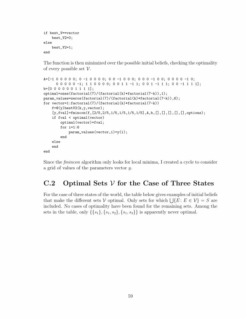
if best_V==vectorbest_V2=0;

elsebest_V2=1;

end

The function is then minimized over the possible initial beliefs, checking the optimalityof every possible set V .

A=[-1 0 0 0 0 0; 0 -1 0 0 0 0; 0 0 -1 0 0 0; 0 0 0 -1 0 0; 0 0 0 0 -1 0;0 0 0 0 0 -1; 1 1 0 0 0 0; 0 0 1 1 -1 1; 0 0 1 -1 1 1; 0 0 -1 1 1 1];

b=[0 0 0 0 0 0 1 1 1 1];optimal=ones(factorial(7)/(factorial(k)*factorial(7-k)),1);param_values=zeros(factorial(7)/(factorial(k)*factorial(7-k)),6);for vector=1:factorial(7)/(factorial(k)*factorial(7-k))

f=@(y)bestV2(k,y,vector);[y,fval]=fmincon(f,[2/5,2/5,1/5,1/5,1/5,1/5],A,b,[],[],[],[],[],options);if fval < optimal(vector)

optimal(vector)=fval;for i=1:6

param_values(vector,i)=y(i);end

elseend

end

Since the fmincon algorithm only looks for local minima, I created a cycle to considera grid of values of the parameters vector y.

C.2 Optimal Sets V for the Case of Three States

For the case of three states of the world, the table below gives examples of initial beliefsthat make the different sets V optimal. Only sets for which

⋃E : E ∈ V = S are

included. No cases of optimality have been found for the remaining sets. Among thesets in the table, only s1, s1, s2, s1, s3 is apparently never optimal.

59

V V Initial beliefsµ(s1) µ(s2) p(s1) p(s2) p(s3) p(S)

2

s1, s2, s3 1/31/3

1/21/4

1/41/10

s1, S 1/31/3

1/31/4

1/41/3

s1, s2, s1, s3 1/51/4

1/201/10

1/101/30

s1, s2, S 3/82/8

1/301/10

1/102/3

3

s1, s2, s3 1/31/3

2/32/3

2/31/4

s1, s2, s1, s3 1/101/5

1/41/2

1/31/5

s1, s2, S 1/31/3

1/31/3

1/61/2

s1, s1, s2, s1, s3 - - - - - -s1, s1, s2, s2, s3 2/5

2/51/2

1/31/3

1/10

s1, s1, s2, S 1/201/20

1/101/10

1/101/10

s1, s2, s3, S 1/21/3

1/31/3

1/31/3

s1, s2, s1, s3, s2, s3 1/31/3

1/61/6

1/61/6

s1, s2, s1, s3, S 1/61/2

1/61/3

1/31/6

4

s1, s2, s3, s1, s2 1/31/3

1/31/3

1/21/10

s1, s2, s3, S 1/31/3

1/21/2

1/21/3

s1, s2, s1, s2, s1, s3 1/101/10

1/61/4

1/101/10

s1, s2, s1, s2, S 1/101/10

1/61/6

1/31/3

s1, s2, s1, s3, s2, s3 2/52/5

1/21/2

1/61/20

s1, s2, s1, s3, S 1/52/5

1/21/2

1/61/3

s1, s1, s2, s1, s3, s2, s3 1/21/4

1/31/10

1/101/10

s1, s1, s2, s1, s3, S 1/51/3

1/61/6

1/61/3

s1, s1, s2, s2, s3, S 1/21/4

1/31/10

1/101/3

s1, s2, s1, s3, s2, s3, S 1/31/3

1/101/10

1/101/3

5

s1, s2, s3, s1, s2, s1, s3 1/51/5

1/51/2

1/21/6

s1, s2, s3, s1, s2, S 1/51/5

1/51/3

1/31/3

s1, s2, s1, s2, s1, s3, s2, s3 1/51/5

1/51/2

1/61/6

s1, s2, s1, s2, s1, s3, S 1/51/5

1/51/2

1/61/3

s1, s2, s1, s3, s2, s3, S 2/51/5

1/51/3

1/61/3

s1, s1, s2, s1, s3, s2, s3, S 1/52/5

1/31/6

1/61/3

6s1, s2, s3, s1, s2, s1, s3, s2, s3 1/3

1/31/3

1/31/3

1/10

s1, s2, s3, s1, s2, s1, s3, S 1/31/3

1/41/3

1/21/4

s1, s2, s1, s2, s1, s3, s2, s3, S 1/31/3

1/41/4

1/101/3

60

Bibliography

[1] Bruno de Finetti. La prevision: ses lois logiques, ses sources subjectives. Annalesde l’Institut Henri Poincare, 7:1–68, 1937.

[2] Jurgen Eichberger, Simon Grant, and David Kelsey. Updating choquet beliefs.Journal of Mathematical Economics, 43(7-8):888–899, 2007.

[3] Larry G. Epstein and Martin Schneider. IID: Independently and indistinguish-ably distributed. Journal of Economic Theory, 113(1):32–50, 2003.

[4] Larry G. Epstein and Kyoungwon Seo. Symmetry of evidence without evidenceof symmetry. Theoretical Economics, 5(3):313–368, 2010.

[5] Ido Erev, Thomas S. Wallesten, and David V. Budescu. Simultaneous over- andunderconfidence: The role of error in judgment processes. Psychological Review,101(3):519–527, 1994.

[6] Pablo I. Fierens and Terrence L. Fine. Toward a chaotic probability model forfrequentist probability: The univariate case. In ISIPTA ’03 Proceedings, pages245–259, 2003.

[7] P.I. Fierens, L.C. Rego, and T.L. Fine. A frequentist understanding of sets ofmeasures. Journal of Statistical Planning and Inference, 139:1879–1892, 2009.

[8] Baruch Fischhoff, Paul Slovich, and Sarah Lichtenstein. Knowing with certainty:The appropriateness of extreme confidence. Journal of Experimental Psychology:Human Perception and Performance, 3(4):552–564, 1077.

[9] Itzhak Gilboa and David Schmeidler. Maxmin expected utility with non-uniqueprior. Journal of Economic Theory, 18(2):141–153, 1989.

[10] Dale Griffin and Amos Tversky. The weighing of evidence and the determinantsof confidence. Cognitive Psychology, 24:411–435, 1992.

[11] Eran Hanany and Peter Klibanoff. Updating preferences with multiple priors.Theoretical Economics, 2(3):261–298, 2007.

[12] Lawrence D. Phillips and Ward Edwards. Conservatism in a simple probabilityinference task. Journal of Experimental Psychology, 72(3):346–354, 1966.

61

[13] Cesaltina P. Pires. A rule for updating ambiguous beliefs. Theory and Decision,53:137–152, 2002.

[14] Eran Shmaya and Leeat Yariv. Foundations for bayesian updating. CaliforniaInstitute of Tech- nology working paper, 2008.

[15] Tan Wang. Conditional preferences and updating. Journal of Economic Theory,108:286–321, 2003.

[16] Chee Yap. Fundamental Problems in Algorithmc Algebra. Oxford UniversityPress, 2000.

62