three essays about energy prices and energy markets
TRANSCRIPT

Graduate Theses Dissertations and Problem Reports
2018
Three Essays about Energy Prices and Energy Markets Three Essays about Energy Prices and Energy Markets
Mousa Tafweeq
Follow this and additional works at httpsresearchrepositorywvueduetd
Recommended Citation Recommended Citation Tafweeq Mousa Three Essays about Energy Prices and Energy Markets (2018) Graduate Theses Dissertations and Problem Reports 7235 httpsresearchrepositorywvueduetd7235
This Dissertation is protected by copyright andor related rights It has been brought to you by the The Research Repository WVU with permission from the rights-holder(s) You are free to use this Dissertation in any way that is permitted by the copyright and related rights legislation that applies to your use For other uses you must obtain permission from the rights-holder(s) directly unless additional rights are indicated by a Creative Commons license in the record and or on the work itself This Dissertation has been accepted for inclusion in WVU Graduate Theses Dissertations and Problem Reports collection by an authorized administrator of The Research Repository WVU For more information please contact researchrepositorymailwvuedu
Three Essays about Energy Prices and Energy Markets
Mousa Tafweeq
Dissertation submitted to the
Davis College of Agriculture Natural Resources and Design
at West Virginia University
in partial fulfillment of the requirements
for the degree of
Doctor of Philosophy
in
Natural Resource Economics
Alan R Collins PhD Committee Chair
Adam Nowak PhD
Stratford Douglas PhD
Xiaoli Etienne PhD
Levan Elbakidze PhD
Division of Resource Economics and Management
Morgantown West Virginia
2018
Keywords energy prices stock markets spatial panel data coal consumption CO2 emissions
Copyright 2018 Mousa Tawfeeq
Abstract
Three Essays about Energy Prices and Energy Markets
Mousa Tafweeq
In this dissertation three related issues concerning empirical time series and panel
models for three essays in energy economics will be investigated The overall theme of these
essays is to explore the relationships between the use of and prices for fossil fuels (coal crude
oil and natural gas) along with larger societal issues of stock market changes resource
extraction rates and CO2 emissions The three main questions will be addressed (1) how do
crude oil prices affect stock markets (2) how have the dynamic linkages between the coal
market and natural gas prices changes with the shale gas revolution and (3) how have
urbanization and other factors impacted CO2 emissions For each question it is considered
proper econometric models to provide empirical answers which will contribute either to the
academic literature or energy economics and policy
In the first essay we investigate linkages between oil price changes and stock market
capitalization in Middle Eastern (ME) economies from 2000-2015 This essay examines how oil
price changes influence stock market capitalization by using a variety of econometric models
including structural breaks VECM VAR and IRF These results suggest the existence of
positive and significant impacts of oil price on MC for all oil-exporting economies
The second essay introduces the idea of a dynamic relationship between coal plus-natural
gas prices and their impacts on coal consumption and extraction In this essay we adopt an
Autoregressive Distributed Lag (ARDL) model to investigate the short-run and long -run
characteristics of coal demand in the US from 2000-2016 Methods and data in this research
contribute to the literature on how the natural gas revolution affects the coal industry in the US
The findings show that coal and natural gas are substitutes as energy sources in the US energy
market Moreover income elasticity reveals that coal is an inferior source of energy since
economic growth has a negative impact on coal demand in the long run Solar energy and
weather both have significant negative impacts on coal consumption over the entire time period
Results provide theoretical and empirical methods of the coal market and allow for a better
understanding of its factors Also these results support the policies to substitute natural gas for
coal due to coal-natural gas prices efficiency and environment friendly
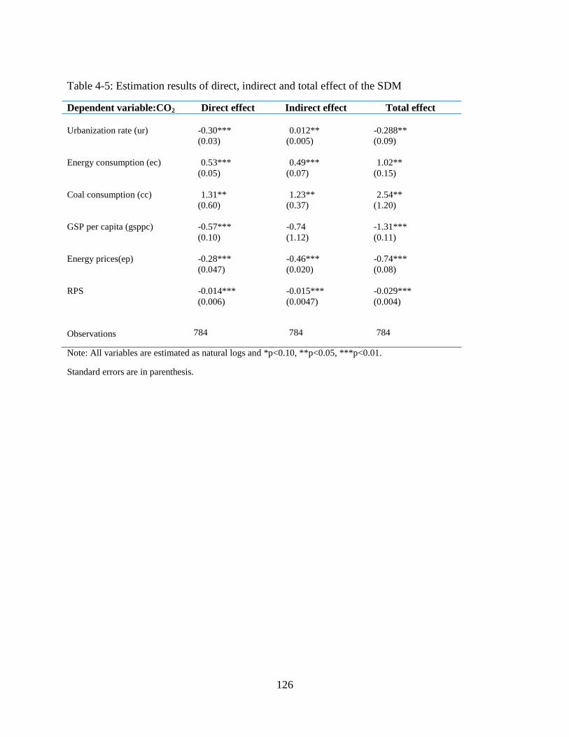
The final essay combines the issues of urbanization energy consumption coal use
energy prices and CO2 emissions regarding US fossil fuel consumption Fossil fuels make up
more than 80 of the humanlsquos energy use (US EIA 2016) and more than 75 of fossil fuels
are used in urban areas Therefore dynamic long- run linkages between fossil fuel energy use
and urbanization are of importance to energy policy makers across the globe This essay focuses
on spillover impacts of energy consumption on CO2 emissions by using spatial autoregressive
regression (SAR) spatial error model (SEM) and spatial dynamic model (SDM) Negative
direct and positive indirect effects of urbanization on state level CO2 emissions are found along
with the negative effects of income along with renewable portfolio standards (RPS) on state level
emissions The income effects provide additional support for the Environmental Kuznets Curve
on CO2 emissions such that income growth reduces per capita CO2 emissions at an own state
level For RPS however the indirect effects of CO2 emission reductions are as large as the own
state direct effects indicating that cross border impacts are important Both of these results are
important due to the prominence of state and local government actions in climate change
mitigation now that the federal government has withdrawn from the Paris Climate Accords
DEDICATION
I would like dedicate this work to Sharmin and Dlovan for providing me with the
unconditional love and support throughout all of my pursuits My Mom who had dedicated her
life to entire family My younger brother who sacrificed his life for humanity and dignity
iv
ACKNOWLEDGEMENTS
I am very grateful for the support and guidance I have received from my family and
faculty throughout my entire graduate career I would like to extend a special thanks to my
advisor Dr Alan Collins for his support and guidance throughout my time at WVU I also wish
to thank Dr Gerard DlsquoSouza Dr Levan Elbakizde Dr Xiaoli Etienne Dr Stratford Douglas
and Dr Adam Nowak for providing me with invaluable advice and assistance through this
process Finally I would also like to thank my fellow grad students for with whom I have spent
countless hours studying with and listening to my ideas on economics energy economics and
the future of natural resource economics
v
Table of Contents
Title Pagehellipi
Abstracthellipii
Dedicationhelliphellipiv
Acknowledgementshelliphelliphellip v
List of Figureshelliphellipvii
List of Tableshelliphellipviii
CHAPTER 1 Introductionhelliphelliphelliphelliphelliphelliphelliphelliphelliphelliphelliphelliphelliphelliphelliphelliphelliphelliphelliphelliphelliphelliphelliphellip1
CHAPTER 2- Essay 1 Linking Crude Oil Prices and Middle East Stock Marketshellip5
1 Introductionhelliphelliphelliphelliphelliphelliphelliphelliphelliphelliphelliphelliphelliphelliphelliphelliphelliphelliphelliphelliphelliphelliphelliphelliphelliphelliphelliphelliphellip5
2 Literature Reviewhelliphelliphelliphelliphelliphelliphelliphelliphelliphelliphelliphelliphelliphelliphelliphelliphelliphelliphelliphelliphelliphelliphelliphelliphellip9
3 Theoryhelliphelliphelliphelliphelliphelliphelliphelliphelliphelliphelliphelliphelliphelliphelliphelliphelliphelliphelliphelliphelliphelliphelliphelliphelliphelliphelliphelliphelliphellip11
4 Methodologyhelliphelliphelliphelliphelliphelliphelliphelliphelliphelliphelliphelliphelliphelliphelliphelliphelliphelliphelliphelliphelliphelliphelliphelliphelliphelliphelliphellip14
5 Data and Descriptive Statisticshelliphelliphelliphelliphelliphelliphelliphelliphelliphelliphelliphelliphelliphelliphelliphelliphelliphelliphelliphelliphelliphellip20
6 Results and Discussion helliphelliphelliphelliphelliphelliphelliphelliphelliphelliphelliphelliphelliphelliphelliphelliphelliphelliphelliphelliphelliphelliphelliphelliphellip22
7 Conclusionshelliphelliphelliphelliphelliphelliphelliphelliphelliphelliphelliphelliphelliphelliphelliphelliphelliphelliphelliphelliphelliphelliphelliphelliphelliphelliphelliphelliphellip28
8 Referenceshelliphelliphelliphelliphelliphelliphelliphelliphelliphelliphelliphelliphelliphelliphelliphelliphelliphelliphelliphelliphelliphelliphelliphelliphelliphelliphelliphelliphelliphellip32
Chapter 3- Essay 2 The Dynamic Response of Coal Consumption to Energy Prices and
GDP An ARDL Approach to the UShelliphelliphelliphelliphelliphelliphelliphelliphelliphelliphelliphelliphelliphelliphelliphelliphelliphelliphelliphellip52
1 Introduction helliphelliphelliphelliphelliphelliphelliphelliphelliphelliphelliphelliphelliphelliphelliphelliphelliphelliphelliphelliphelliphellip52
2 Literature Reviewhelliphelliphelliphelliphelliphelliphelliphelliphelliphelliphelliphelliphelliphelliphelliphelliphelliphelliphelliphelliphelliphelliphelliphelliphelliphelliphellip57
3 Methodology helliphelliphelliphelliphelliphelliphelliphelliphelliphelliphelliphelliphelliphelliphelliphelliphelliphelliphelliphelliphelliphelliphelliphelliphelliphelliphelliphelliphellip59
4 Datahelliphelliphelliphelliphelliphelliphelliphelliphelliphelliphelliphelliphelliphelliphelliphelliphelliphelliphelliphelliphelliphelliphelliphelliphelliphelliphelliphelliphelliphelliphelliphellip64
5 Results helliphelliphelliphelliphelliphelliphelliphelliphelliphelliphelliphelliphelliphelliphelliphelliphelliphelliphelliphelliphelliphelliphelliphelliphelliphelliphelliphelliphelliphelliphellip67
6 Conclusions helliphelliphelliphelliphelliphelliphelliphelliphelliphelliphelliphelliphelliphelliphelliphelliphelliphelliphelliphelliphelliphelliphelliphelliphelliphelliphelliphelliphellip74
7 Referenceshelliphelliphelliphelliphelliphelliphelliphelliphelliphelliphelliphelliphelliphelliphelliphelliphelliphelliphelliphelliphelliphelliphelliphelliphelliphelliphelliphelliphelliphellip77
Chapter 4- Essay 3 The Spillover Impacts of Urbanization and Energy Usage on CO2
Emissions Patterns in the US helliphelliphelliphelliphelliphelliphelliphelliphelliphelliphelliphelliphelliphelliphelliphelliphelliphelliphelliphelliphelliphelliphellip88
1 Introduction helliphelliphelliphelliphelliphelliphelliphelliphelliphelliphelliphelliphelliphelliphelliphelliphelliphelliphelliphelliphelliphelliphelliphelliphelliphelliphelliphelliphellip88
2 Literature Reviewhelliphelliphelliphelliphelliphelliphelliphelliphelliphelliphelliphelliphelliphelliphelliphelliphelliphelliphelliphelliphelliphelliphelliphelliphelliphelliphellip93
3 Theoretical Modelhelliphelliphelliphelliphelliphelliphelliphelliphelliphelliphelliphelliphelliphelliphelliphelliphelliphelliphelliphelliphelliphelliphelliphelliphelliphelliphellip98
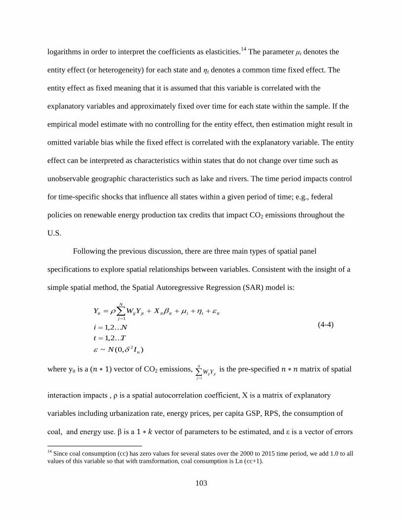
4 Empirical Modelhelliphelliphelliphelliphelliphelliphelliphelliphelliphelliphelliphelliphelliphelliphelliphelliphelliphelliphelliphelliphelliphelliphelliphelliphelliphelliphellip102
5 Datahelliphelliphelliphelliphelliphelliphelliphelliphelliphelliphelliphelliphelliphelliphelliphelliphelliphelliphelliphelliphelliphelliphelliphelliphelliphelliphelliphelliphelliphelliphelliphelliphellip106
6 Results and Discussionhelliphelliphelliphelliphelliphelliphelliphelliphelliphelliphelliphelliphelliphelliphelliphelliphelliphelliphelliphelliphelliphelliphelliphelliphellip109
7 Conclusions helliphelliphelliphelliphelliphelliphelliphelliphelliphelliphelliphelliphelliphelliphelliphelliphelliphelliphelliphelliphelliphelliphelliphelliphelliphelliphelliphelliphelliphellip114
8 Referenceshelliphelliphelliphelliphelliphelliphelliphelliphelliphelliphelliphelliphelliphelliphelliphelliphelliphelliphelliphelliphelliphelliphelliphelliphelliphelliphelliphelliphelliphellip116
Chapter 5 Conclusionshelliphelliphelliphelliphelliphelliphelliphelliphelliphelliphelliphelliphelliphelliphelliphelliphelliphelliphelliphelliphelliphelliphelliphelliphellip127
vi
List of Figures
Essay 1
Figure 21 Mechanisms of crude oil price changes on an oil importer stock market increase (left
arrow) and decrease (right arrow)helliphelliphelliphelliphelliphelliphelliphelliphelliphelliphelliphelliphelliphelliphelliphelliphelliphelliphelliphelliphelliphelliphellip13
Figure 2-2 Market capitalization (MC in billion USD) and crude oil price (OP in USD)helliphellip47
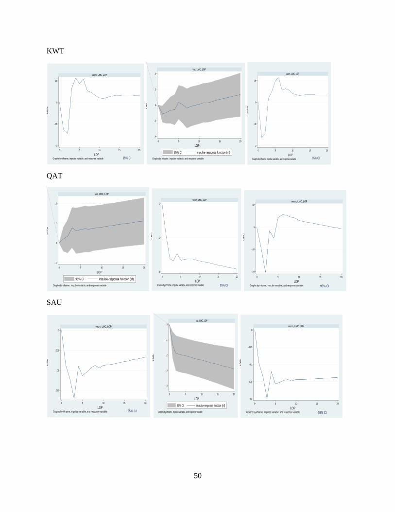
Figure2-3 Impulse response function (IRF) for each Middle East economyhelliphelliphelliphelliphelliphelliphellip48
Essay 2
Figure 3-1 US power generation from coal and natural gashelliphelliphelliphelliphelliphelliphelliphelliphelliphelliphelliphelliphellip54
Figure 3-2 Coal producing states and change in coal productionhelliphelliphelliphelliphelliphelliphelliphelliphelliphelliphellip55
Figure 3-3 Economic growth (US$)helliphelliphelliphelliphelliphelliphelliphelliphelliphelliphelliphelliphelliphelliphelliphelliphelliphelliphelliphelliphelliphelliphellip83
Figure 3-4 Coal consumption (MBTU)helliphelliphelliphelliphelliphelliphelliphelliphelliphelliphelliphelliphelliphelliphelliphelliphelliphelliphelliphelliphellip83
Figure 3-5 Coalndashnatural gas prices ($MBTU)helliphelliphelliphelliphelliphelliphelliphelliphelliphelliphelliphelliphelliphelliphelliphelliphelliphellip83
Figure 3-6 Heating degree-dayshelliphelliphelliphelliphelliphelliphelliphelliphelliphelliphelliphelliphelliphelliphelliphelliphelliphelliphelliphelliphelliphelliphelliphellip83
Figure 3-7 Cooling degree-dayshelliphelliphelliphelliphelliphelliphelliphelliphelliphelliphelliphelliphelliphelliphelliphelliphelliphelliphelliphelliphelliphelliphelliphellip84
Figure 3-8 Solar consumption (TBTU)helliphelliphelliphelliphelliphelliphelliphelliphelliphelliphelliphelliphelliphelliphelliphelliphelliphelliphelliphelliphelliphellip84
Figure 3-9 Plot of the cumulative sum of recursive residuals (CUSUM)helliphelliphelliphelliphelliphelliphelliphellip84
Figure 3-10 Impulse response function (combined)helliphelliphelliphelliphelliphelliphelliphelliphelliphelliphelliphelliphelliphelliphelliphelliphellip85
Panel A 2000 to 2016 Datahelliphelliphelliphelliphelliphelliphelliphelliphelliphelliphelliphelliphelliphelliphelliphelliphelliphelliphelliphelliphelliphelliphelliphelliphelliphellip85
Panel B 2000 to 2008 Datahelliphelliphelliphelliphelliphelliphelliphelliphelliphelliphelliphelliphelliphelliphelliphelliphelliphelliphelliphelliphelliphelliphelliphelliphelliphellip86
Panel C 2009 to 2016 Datahelliphelliphelliphelliphelliphelliphelliphelliphelliphelliphelliphelliphelliphelliphelliphelliphelliphelliphelliphelliphelliphelliphelliphelliphelliphellip86
Essay 3
Figure 4-1 Urban and rural populations of the world 1950ndash2050helliphelliphelliphelliphelliphelliphelliphelliphelliphellip88
Figure 4-2 CO2 emissions from 1750 and projected to 2050helliphelliphelliphelliphelliphelliphelliphelliphelliphelliphelliphellip88
vii
List of Tables
Essay 1
Table 2-1 Macroeconomic overview of ME regionhelliphelliphelliphelliphelliphelliphelliphelliphelliphelliphelliphelliphelliphelliphelliphellip37
Table 2-2 Descriptive statistics for MC (billion USD) and for OP (USD per barrel)helliphelliphellip37
Table 2-3 Tests for unit root hypothesis for market capitalization and oil pricehelliphelliphelliphelliphellip38
Table 2-4 Selection of optimum lag according AIC and BIC criteriahelliphelliphelliphelliphelliphelliphelliphelliphellip39
Table 2-5 Tests of cointegration for MC and OPhelliphelliphelliphelliphelliphelliphelliphelliphelliphelliphelliphelliphelliphelliphelliphelliphellip39
Table 2-6 The result of VECM for MC and OP 2001-2008helliphelliphelliphelliphelliphelliphelliphelliphelliphelliphelliphelliphellip40
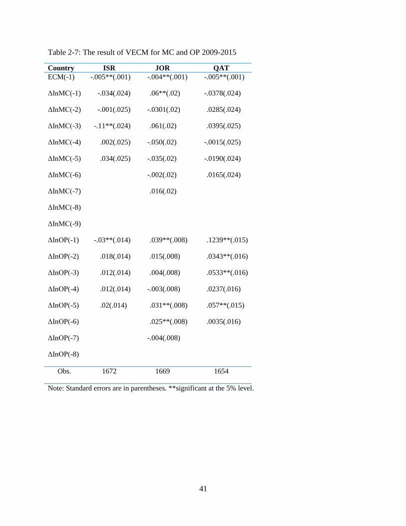
Table 2-7 The result of VECM for MC and OP 2009-2015helliphelliphelliphelliphelliphelliphelliphelliphelliphelliphelliphelliphellip41
Table 2-8 The result of VECM for MC and OP 2001-2015helliphelliphelliphelliphelliphelliphelliphelliphelliphelliphelliphellip42
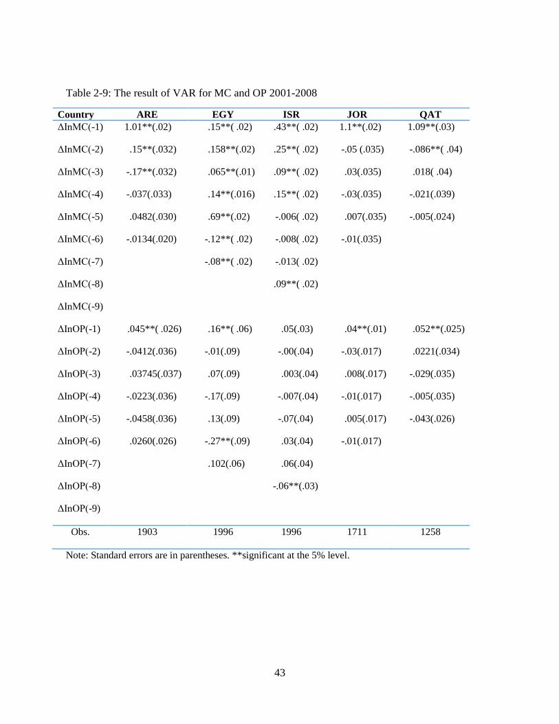
Table 2-9 The result of VAR for MC and OP 2001-2008helliphelliphelliphelliphelliphelliphelliphelliphelliphelliphelliphelliphelliphellip43
Table 2-10 The result of VAR for MC and OP 2009-2015helliphelliphelliphelliphelliphelliphelliphelliphelliphelliphelliphelliphellip44
Table 2-11 The result of VAR for MC and OP 2001-2015helliphelliphelliphelliphelliphelliphelliphelliphelliphelliphelliphelliphellip45
Table 2-12 Summary of resultshelliphelliphelliphelliphelliphelliphelliphelliphelliphelliphelliphelliphelliphelliphelliphelliphelliphelliphelliphelliphelliphelliphelliphellip46
Essay 2
Table 3-1 Descriptive statisticshelliphelliphelliphelliphelliphelliphelliphelliphelliphelliphelliphelliphelliphelliphelliphelliphelliphelliphelliphelliphelliphelliphelliphellip80
Table 3-2 Tests for unit root testhelliphelliphelliphelliphelliphelliphelliphelliphelliphelliphelliphelliphelliphelliphelliphelliphelliphelliphelliphelliphelliphelliphelliphellip80
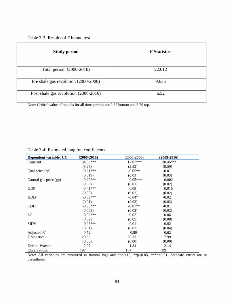
Table 3-3 Results of F bound testhelliphelliphelliphelliphelliphelliphelliphelliphelliphelliphelliphelliphelliphelliphelliphelliphelliphelliphelliphelliphelliphelliphellip81
Table 3-4 Estimated long run coefficientshelliphelliphelliphelliphelliphelliphelliphelliphelliphelliphelliphelliphelliphelliphelliphelliphelliphelliphelliphellip81
Table 3-5 Estimated short run coefficientshelliphelliphelliphelliphelliphelliphelliphelliphelliphelliphelliphelliphelliphelliphelliphelliphelliphelliphellip82
Table 3-6 Diagnostic tests statisticshelliphelliphelliphelliphelliphelliphelliphelliphelliphelliphelliphelliphelliphelliphelliphelliphelliphelliphelliphelliphelliphelliphellip82
Essay 3
Table 4-1 Descriptive statisticshelliphelliphelliphelliphelliphelliphelliphelliphelliphelliphelliphelliphelliphelliphelliphelliphelliphelliphelliphelliphelliphelliphelliphellip123
Table 4-2 Post diagnostic tests helliphelliphelliphelliphelliphelliphelliphelliphelliphelliphelliphelliphelliphelliphelliphelliphelliphelliphelliphelliphelliphelliphelliphellip123
Table 4-3 Estimation results of non-spatial- panel data modelshelliphelliphelliphelliphelliphelliphelliphelliphelliphelliphellip124
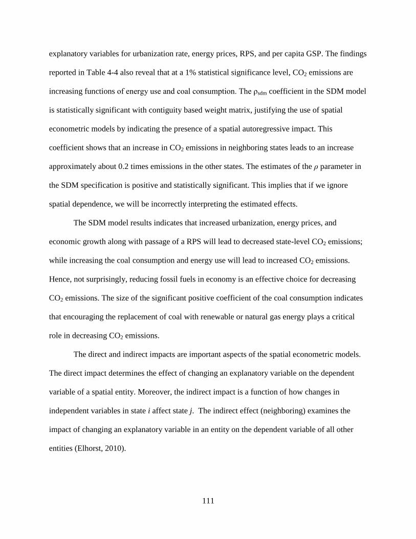
Table 4-4 Estimation results of spatial- panel data modelshelliphelliphelliphelliphelliphelliphelliphelliphelliphelliphelliphelliphellip125
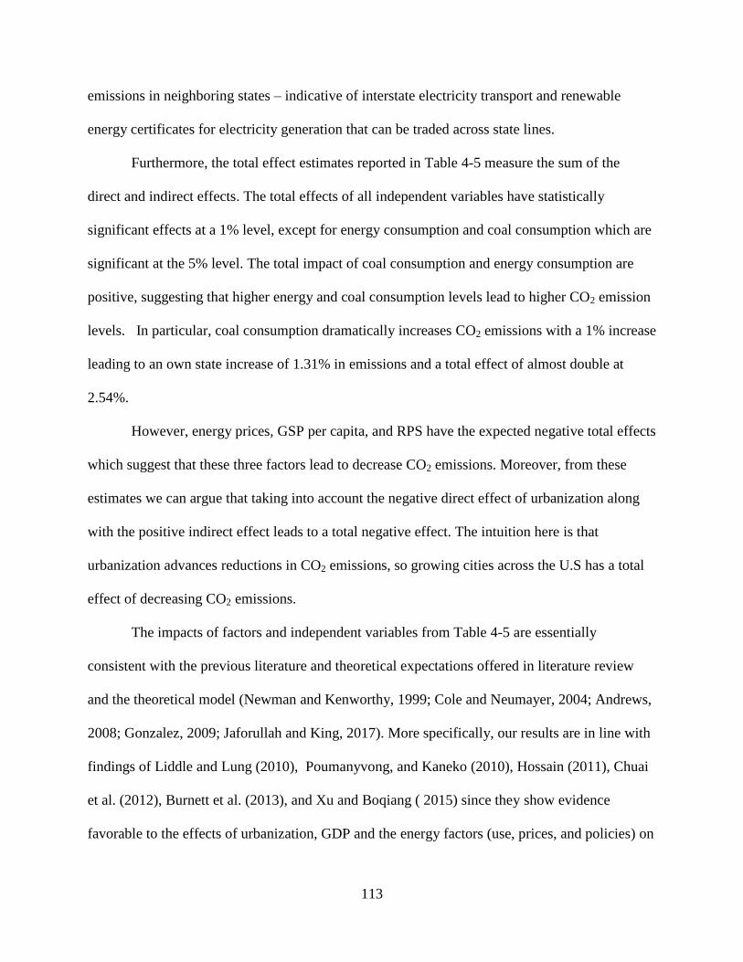
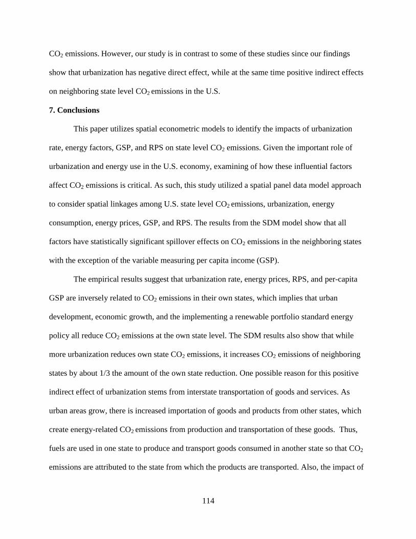
Table 4-5 Estimation results of direct indirect and total effect of the SDMhelliphelliphelliphelliphelliphelliphellip126
viii
1
Chapter 1 Introduction
Economists consider profoundly about energy price volatilities stock markets and
energy consumption as vital parts of an economy In the face of challenges and opportunities in
the energy market crude oil prices and energy markets and urbanization have become concerns
of the global community (Hamilton 2003 Kilian 2006 Poumanyvong and Shinji 2010 Teulon
2015 Xu and Boqiang 2015) To address these concerns many economists are paying attention
to the dynamic linkages between oil price and the stock market value between coal and natural
gas prices and coal consumption and among urbanization energy factors and CO2 emissions
(Sadorsky 2006 York 2003 Sadorsky 2014 Burnett etal 2013) The three research studies
cover the impact of economic and policy analysis on energy and environmental economics They
include crude oil prices and stock market in the Middle Eastern economies the link between coal
or natural gas prices and coal consumption in the US and urbanization energy use and CO2
emissions in the US In these essays a variety of non-spatial and spatial econometric models are
utilized to identify links among variables
Chapter two focuses on dynamic linking between crude oil prices and stock market
capitalization The economy of the Middle East (ME) region is diverse in nature composed of 17
countries which includes both oil exporting and importing countries The economies of this
region depend heavily on hydrocarbon reserves Major oil exporting economies in this region
include Iraq Saudi Arabia Qatar Bahrain Oman Yemen UAE Kurdistan region Kuwait and
Iran In this essay we investigate nine ME economies including oil-exporting and oil-importing
since there is no accurate data for other eight countries and authorities In the oil-exporting
economies a significant portion of total GDP comes from hydrocarbon exports More
importantly ME oil exporters rely heavily on oil prices as shown by fluctuations in economic
2
performance when oil prices change The negative impact of oil price volatility has affected
structural reform initiatives in ME economies to achieve stability and sustainability of economic
growth (Dasgupta et al 2002) Moreover increasing the role of stock market and crude oil have
been the vital part of in the ME economies and stock market activities in this region Given these
facts it is reasonable to suspect that crude oil prices have economic and financial effects within
countries of the ME yet little is known about these impacts in the ME region Therefore the
main objective of this study is to show whether the oil prices changes impact stock market
capitalization in economies across this region
Chapter three examines US coal consumption and the impacts of prices (coal and
natural gas) weather and economic growth on the use of this resource In recent years the coal
industry has faced decreasing production with the resultant negative effects on job markets and
incomes in the coal producing states While arguably cleaner than coal natural gas is a possible
substitute to coal since it is more efficient and less emits environment than coal Moreover coal
industry is in a crisis condition in the US is receiving significant attention recently Since fuel
choice for power generation relies on fuel prices using ARDL model we investigate the
dynamic short and long-run correlations between coal consumption natural gas price price of
coal and other factors over time period 2000-2016 The findings show that there exist long-run
relationships among variables Coal and natural gas prices have negative and positive linkages
with consumption of coal respectively
Chapter four examines spillover effects of urbanization and energy factors on explaining
state level CO2 emissions A number of previous studies have noted the geographic
neighborhood and location in CO2 emissions (Conley and Ligon 2002) Chuai et al 2012 Yu
2012 Burnett et al 2013) Thus we model the issue of CO2 emissions using spatial
3
econometric methods Given the potential spatial correlations between CO2 emissions and state
level independent variables we utilize models Spatial Autoregressive Regression (SAR) Spatial
Error (SEM) and Spatial Durbin (SDM) Results suggest that coal consumption and energy use
have larger effects on CO2 emissions than energy prices urbanization GSP and RPS Further
urbanization has a negative direct impact on own state CO2 emissions but positive indirect
effects on emissions in neighboring states
This dissertation takes a comprehensive view of the energy prices energy market and
CO2 emissions examining both US and ME economies Historically coal extraction and its
consumption have been dominant in the electricity energy market The final essay attempts to
better understand what roles coal and natural gas prices have played in the decline of coal
production while controlling for weather and renewable energy Here we model coal
consumption and evaluate how the dynamic relationships have changed since the development of
shale gas1 In the fourth chapter we focus on the spillover effects that state level energy factors
and GSP have on per capita CO2 emissions With this dissertation researchers and policymakers
will have a better understanding of the US energy market and the ME stock market value and
can better address the challenges and opportunities offered energy prices and energy prices
The dissertation consists of five chapters including the introduction Chapter 2 offers the
Essay 1 that examines dynamic linking between oil price changes and stock market capitalization
in the ME Chapter 3 presents Essay 2 that provides an empirical analysis of how energy prices
weather and income influence coal consumption in the USlsquo energy market Chapter 4 represents
Essay 3 that examines whether the energy factors of state-level affect carbon dioxide emission
1 We explore structural changes in energy markets in all three essays due to recent increases in shale oil and gas
production using hydraulic fracturing technology
4
level is convergence in the US This dissertation concludes in Chapter 5 with directions for
future research
5
Chapter 2 - Essay 1 Linking Crude Oil Prices and Middle East Stock Markets
1 Introduction
Due to the vital role of crude oil in the global economy there has been a vast amount of
studies intended to determine how crude oil price changes impact world economies and financial
markets A large number research studies have found that there exists statistically significant
impacts of crude oil price on economic growth and stock market indicators (Driesprong et al
2008 Jones and Kaul 1996 Narayan and Sharma 2011 Lee et al 2012 Sadorsky
1999 Park and Ratti 2008 Scholtens and Yurtsever 2012 Apergis and Miller 2009 Guumlntner
2013 Kilian and Park 2009 )
Fewer studies have focused on the impact of crude oil price changes on where large
reserves and production of crude oil exist - Middle East (ME) stock markets Moreover there is
no research that links crude oil prices and market capitalization (as a measure of stock market
changes) in the ME economies The economic and financial impacts of crude oil prices have to
be captured by stock market value for they are bound to influence cash flows outstanding
shares and the price of shares in the stock markets Findings from previous research indicate that
crude oil price changes do have a significant impacts on the market performances (Jones et al
2004 Basher and Sadorsky 2006 Miller and Ratti 2009 Filis et al 2011 Arouri and Roult
2012 Le and Chang 2015 Ewing and Malik 2016) In a recent study Ghalayini (2011)
emphasize that crude oil price is an essential element of ME economies The ME economies
have experienced with growth and crisis related to variability in crude oil prices Considering
that there exists in fact an economic effect of the crude oil price volatility should also be
captured by market capitalization in the ME stock markets
Previous empirical studies on crude oil price and stock market activities use stock market
6
returns or stock prices specifications (ie Driesprong et al 2008 Jones and Kaul
1996 Narayan and Sharma 2011 Lee et al 2012 Sadorsky 1999 Park and Ratti
2008 Scholtens and Yurtsever 2012 Park and Ratti 2008 Apergis and Miller 2009 Guumlntner
2013 Kilian and Park 2009) We argue that there are problems with how stock indexes are
calculated that might lead to disadvantages For instance the TA-35 index in Israel is a price-
weighted index which is calculated by taking the sum of the prices of all 35 stocks in the index
Stocks with higher prices have a larger impact on movements in the index as compared to lower-
priced stocks However stock market capitalization (MC) provides the total value of a company
indicating its value in the market and economy By looking at MC a proper evaluation is
provided for the current situation of financial and economic development Furthermore time
series data of MC movements could provide trend to investors as to how the value of companies
in the stock markets In this view MC is a macroeconomic indicator which may allow for policy
makers and investors to make better decisions in an economy
ME stock markets have been affected by crude oil price changes before and after global
financial crisis The ME countries experienced strong economic growth during 2000ndash2008 as a
result of higher oil prices (Selvik and Stenslie 2011) However the global financial crisis has
transformed into a severe financial and economic crisis in most of the ME economies Although
since 2002 the worldlsquos crude oil prices have risen rapidly they have fallen sharply to an even
$35 per barrel recently In November 2007 prices of both WTIlsquos OP and the Brentlsquos OP went
beyond $90 per barrel and the recent record peak of US$145 per barrel reached in July 2008This
resulted in great fluctuations in the OP market causing the ME stock markets to major changes
which in turn changed the financial markets and altered the entire economies of region into
crisis Since many of the ME economies represent the majority of oil-trade ME policymakers
7
must not only take into consideration how their decisions affect energy and oil prices but also
the impact that oil price shocks have on their own stock markets Hence this empirical study
investigates a dynamic linkages between OP and MC in the ME stock markets
In this context the objective of this study is to examine the impact of changes in crude oil
prices (OP) on MC in the stock markets of nine ME economies including a mixture of oil-
exporting and oil-importing economies (United Arab Emirates Bahrain Egypt Israel Jordan
Kuwait Qatar Saudi Arabia and Turkey) Most research referring to crude oil prices and stock
markets concentrates on how various indications of changes of crude oil price could influence
stock market Several studies have examined the impact of the changes of crude oil price on
stock markets However taking account the essential role of crude oil as a major input in
production and supply of goods it is crucial to examine how the prices of crude of oil impacts
market capitalization
In this paper the principal focus is to examine the dynamic long-run linkages between
stock MC and OP across nine ME economies from 2001 to 2015 using a Vector Autoregressive
Regression (VAR) and Vector Error Correction Model (VECM) This study offers the following
contributions to the literature (1) a consideration of and testing for time series (ie unit root
structural break tests misspecification tests and LM test test for normality and test for stability
condition) and econometric models exploring the relationship between OP and stock MC in the
ME region and (2) using daily stock market capitalization which combines all companies in
each country not just subset of index
Our findings suggest four conclusions about the relationship between OP and MC First
the Johansenlsquos test in the period 2001-2008 shows that there are cointegration between OP and
MC in Bahrain Kuwait Saudi Arabia and Turkey and no-cointegration the remaining five
8
economies During the 2009-2015 there are cointegration OP and MC relationship for United
Arab Emirates Israel Jordan and Qatar and no cointegrtaion for the other five economies In
the total period 2001-2015 the results suggest that the existence of a cointegration relationship
among the OP and MC variables in seven of nine countries (Egypt and Jordan are exceptions)
The significant linkages between OP and MC imply some degree of predictability dependency
on oil prices and association between stock market values and crude oil in the ME region
Governments investors and policy makers could have a view to the stock markets in the ME
thus the results may assist them to make a better decision
Second the empirical results of VECM indicate that a dynamic longndashrun response of MC
to an OP increase in all countries except for Israel and Turkey suggesting that all oil-exporting
stock markets examined have long-run dependence on oil prices in all periods Third the
evidence of VAR system show that an increase in OP is associated with a significant increase in
the short-run MC for all economies except Israel Jordan and Egypt in the three time periods
This result emphasizes that oil-exporting countries are more likely depend on oil price increase
in short and long ndashrun periods
Finally the IRFs of response of MC to OP shocks confirm positive relationships between
OP and MC for the majority of ME stock markets These research findings will inform policy
makers in making decisions about the structure and reform of economies in the ME For
instance detecting a particular pattern in changes might assist investors in making decisions
based on both MC and OP In addition the optimal decision for international investors that
invest in the ME and seek to maximize the expected profit of their stocks could be to invest only
when OP has positive effect on MC Therefore these findings not only will be informative for
portfolio investors in building a stock portfolio but also help us understand better the linkages
9
between OP and MC providing us with a clearer picture in the ME economies As a result
observing whether the changes in crude oil prices are transmitted to the ME stock markets will
reconsider attention from the policy makers of the region and the global investors
The remainder of this paper is organized as follows Section 2 surveys relevant literature
on oil price and market capitalization Section 3 provides a theoretical framework for this
research Section 4 is explanation of empirical related to models time series The next section
describes data and presents descriptive statistics Section 6 presents the results and reports
empirical findings in the paper Section 7 concludes
2 Literature Review
Oil prices and stock markets have been a subject of economic and financial research in
the global economy especially during the past decade (Jones et al 2004 Maghyereh 2006
Basher and Sadorsky 2006 Yu and Hassan 2008 Miller and Ratti 2009 Lardic and Mignon
2008 Filis etal 2011 Arouri and Roult 2012 Le and Chang 2015 Ewing and Malik 2016)
Jones et al (2004) address the theoretical and empirical insights of the macroeconomic
consequences of oil price shocks while other studies examine how oil price shocks affect the
performance of stock markets in different economies Using data from different markets and
applying different methodologies many of these studies conclude that there exists a strong
linkage between the oil prices and stock market activities
The linkage between oil prices and stock markets has also become the subject matter of
scholarly studies that address a variety of topics within developed economies Sadorsky (1999)
examines the dynamic interdependence between oil prices and economic activities including
inflation adjusted stock returns in the US Using monthly data from 1947-1996 he showed that
stock returns represented by SampP 500 index had been affected by oil prices and their volatility
Positive shocks to oil prices were found to have negative effects on stock returns On the other
10
hand no effect of stock market returns on oil prices was detected perhaps because oil prices are
formed by global supply and demand forces
Using time series models and a VECM approach Miller and Ratti (2009) examine the
long run relationship between oil prices and stock markets from 1971 to 2008 in six OECD
countries Their results suggest negative linkages between increasing oil prices and stock market
indices for all six economies Abhyankar et al (2013) conducted a study on oil price shocks and
stock market activities for Japanlsquos economy from 1999 to 2011 They concluded with a VAR
model that there was a negative effect on the Japanese stock market as an oil-importing country
Additional research has examined the effect of oil price changes on stock market returns in
emerging countries Basher and Sadorsky (2006) studied the effects of crude oil price changes on
emerging stock market returnsin 21 emerging stock markets around the world including
countries in Middle East Asia South America Europe and Africa Both oil-exporting and oil-
importing countries were included in their study They utilized a multi-factor model that
incorporated both unconditional and conditional risk factors in an approach similar to a capital
asset pricing model Six models investigated the relationships among stock market returns
market risk oil price exchange rate risk squared market price risk and total risk In general
they found strong evidence that oil price was found to have a statistically significant positive
effect on stock market returns in most emerging markets
There is some evidence supporting the link between oil prices and stock markets of the
Gulf Cooperation Council (GCC) within the ME economies Fayyad and Daly (2011) assessed
the effect of oil price shocks on stock markets in GCC countries compared with the US and
United Kingdom (UK) The time series data applied in this research came from weighted equity
market indices of seven stock markets - Kuwait Oman United Arab Emirates (UAE) Bahrain
11
and Qatar along with the UK and US They applied a VAR analysis to examine linkages
between oil price and stock market returns from September 2005 to February 2010 They found
that oil price had statistically significant positive impacts on stock markets in the GCC
economies compared to negative impacts on stock markets in the US and UK These empirical
results suggest that the forecasted influence of oil on stock markets rose with an increase in oil
prices
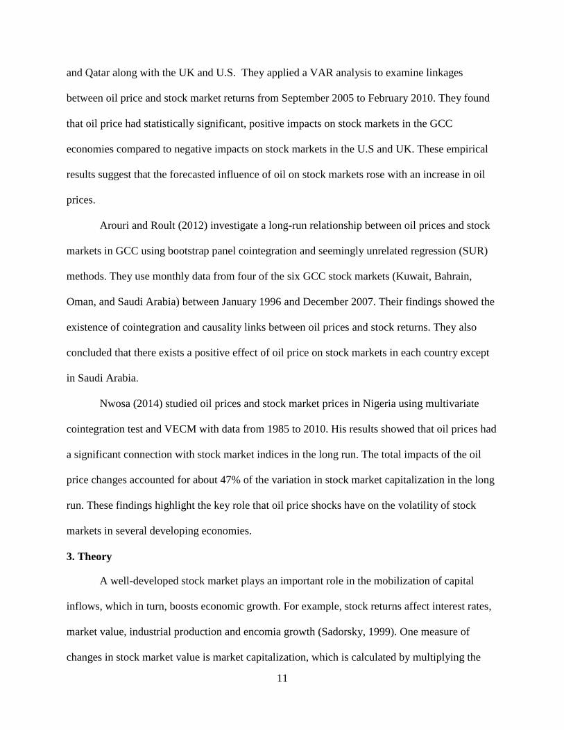
Arouri and Roult (2012) investigate a long-run relationship between oil prices and stock
markets in GCC using bootstrap panel cointegration and seemingly unrelated regression (SUR)
methods They use monthly data from four of the six GCC stock markets (Kuwait Bahrain
Oman and Saudi Arabia) between January 1996 and December 2007 Their findings showed the
existence of cointegration and causality links between oil prices and stock returns They also
concluded that there exists a positive effect of oil price on stock markets in each country except
in Saudi Arabia
Nwosa (2014) studied oil prices and stock market prices in Nigeria using multivariate
cointegration test and VECM with data from 1985 to 2010 His results showed that oil prices had
a significant connection with stock market indices in the long run The total impacts of the oil
price changes accounted for about 47 of the variation in stock market capitalization in the long
run These findings highlight the key role that oil price shocks have on the volatility of stock
markets in several developing economies
3 Theory
A well-developed stock market plays an important role in the mobilization of capital
inflows which in turn boosts economic growth For example stock returns affect interest rates
market value industrial production and encomia growth (Sadorsky 1999) One measure of
changes in stock market value is market capitalization which is calculated by multiplying the
12
per-share price by the number of outstanding shares MC provides a measure of the total value
for companies and entire economy condition For companies in a given economy stock market
capitalization correlates with business development capital accumulation energy and oil prices
and other variables (Maghyereh 2006)
In theory oil price shocks can affect economic activity and economic growth (Brown and
Yuumlcel 2002 Lardic and Mignon 2008 Ghalayini 2011 Gadea etal 2016) On the one hand
stock market activities and MC are affected through both consumption and investment to extract
oil Consumption of goods and services are influenced indirectly by crude oil price related to
income and output (Ewing and Thompson 2007) OP changes can affect output through
production cost effect and then it will impact income (Figure 2-1)
We argue that oil prices have affected income in the world economy in different ways
For a given level of world GDP for instance previous studies found that oil prices have a
negative impact on income in oil-importing countries and positive effects in oil-exporting
economies (Lescaroux and Mignon 2009 Filis etal 2011 Gadea etal 2016) Therefore oil
price is an essential factor to determine firm cash flows and stock market performance (Figure 2-
1) When the price of oil increases income transfers take place from oil-importing economies to
oil-exporting economies and consumption is reduced in oil-importing economies (Lardic and
Mignon 2008 2006) On the other hand crude oil is a significant input in production and GDP
(Jimenez-Rodriguez and Saacutenchez 2006 Lardic and Mignon 2006) Increases in the price of oil
could decrease the demand for petroleum reducing productivity of other inputs which force
companies to lower output Therefore oil price influences economic performance and markets
and thus affects stock market activity and market capitalization
Oil price volatilities lead to changes in stock market returns while stock market returns
13
and cash flows cause changes in market capitalization (Arouri and Roult 2012 Fayyad and
Daly 2011 Abhyankar et al 2013 Ha and Chang 2015 Teulon and Guesmi 2014) Changing
oil prices impact the prices of a wide range of commodities including inputs to industrial (eg
chemicals and electricity) and transportation sectors The overall net impact of oil prices on stock
market capitalization relies on a complex combination of cash flow impacts and then market
capitalization in stock market As shown in Figure 2-1 oil price changes can effect stock market
capitalization through multiple pathways In this figure oil-importing countries experience
decreased output with from production cost increases due to oil price decreases Increased crude
oil prices also raises the inflation rate via higher prices throughout the economy The
consequences of decreasing output decreases income levels increases cost of living and reduces
consumption Additional impacts of increased inflation include higher discount rates in the
economy The end result of these changes in the economy is that firm cash flows will decrease
thereby leading to declining market capitalization
Figure 21 Mechanisms of crude oil price changes on an oil importer stock market increase (left
arrow) and decrease (right arrow)
14
Thus more formally expressed stock market capitalization is strictly a function of
discounted cash flows and discounted cash flows are function of oil prices macroeconomic
activities and socio-political variables
)( tt DCFMMC (2-1)
)( ttt XOPODCF (2-2)
Where MCt represent the value of stock market capitalization DCFt is the discounted sum of
expected future cash flows Xt represents macroeconomic activities (ie interest rate or shale
oil production) and OPt is oil prices Oil price fluctuations impact corporate output and
earnings domestic prices and stock market share prices
4 Methodology
A variety econometric methods have been utilized in the past decade to examine the
impact of oil price shocks on the stock market In order to comprehensively explore the linkages
between OP and MC in ME economies we use time series methods including unit root tests
multivariate time series VECM and VAR analysis A VAR model is utilized to examine all
variables as jointly endogenous and does not inflict restrictions on the structural relationship
VECM is a restricted VAR that has cointegration restrictions Thus the VECM specification
restricts the long-run trend of the endogenous variables to converge to their cointegrating
linkages while allowing a wide range of short-run dynamics
41 Unit Root Testing
The first step of any time series analysis is to examine the order of integration for all
variables used In this analysis Augmented Dickey Fuller (ADF) (Dickey and Fuller 1981) and
Phillips and Perron (1988) (PP) tests were applied to examine the unit roots and the stationary
15
properties of oil price and stock market capitalization variables Equation (3) was used to
calculate the test statistics for both the OP and MC variables
∆119884119905 = 120572 + 120573119905 + 120574119910119905minus1 + 120575∆119910119905minus119894 + 휀119905119901119894=1 (2-3)
In Equation (2-3) 119910119905 stands for either the OP or MC variable 120572 is the constant term 120573 the
coefficient of time trend 휀119905 denotes the error term and p is the number of lags determined by the
auto regressive process From this equation the H0 γ = 0 ie 119910 has a unit root against the
alternative hypothesis of H1 γ lt 0 ie 119910119905 is stationary Observations from the majority of
economic time series data studies are non-stationary at levels but when first difference is
considered the series become stationary (Engle and Granger 1987) After confirmation of the
stationarity of variables we examine whether there exists any long run relationship with the
Johansen and Juselius (JJ) cointegration test
In this study a Zivot-Andrews (ZA) test was utilized Zivot and Andrews (1992)
describe a unit root test for a time series that allows for one structural break in the series
Structural breaks might appear in the trend intercept or both The ZA test detects unknown
structural breaks in the time series A break date is chosen where the t-statistic from the ADF test
of a unit root is at a minimum level or negative Thus a break date can be selected where the
evidence is less suitable for the null of a unit root According to the process described in Zivot
and Andrews (1992) a breakpoint can be endogenously verified
42 Johansenrsquos Cointegration Method
One of the principal objectives in a time series approach is to estimate a long-run
equilibrium using a systems-based method (Johansen 1988 1991 1992 and 1995 Dolado et
al 1990 and Johansen and Juselius 1990) The Johansenlsquos estimation method is represented by
Equation (2-4)
16
∆119910119905 = 1198600 + П119910119905minus1 + 120490119894∆119910119905minus119894 + 휀119905119903119894minus1 (2-4)
Where yt denotes 2x1 vector containing the OP and MC variables Long-run relationships are
captured through П matrix (n x r) in which n is the number of variables and r is the number of
cointegrating vectors can be written as П = αβ where β is matrix of cointegrating vectors α is
adjustment confidents (Johansen 1991) 120490119894 is a matrix with coefficients associated to short-run
dynamic effects The matrix α consists of error correction coefficients and r is the number of
cointegrating relationships in the variable (0ltrltn) which is also known as speed of adjustment
parameter β is a matrix of r cointegrating vectors which represent the long run relationship
between variables The optimum lag is selected on the basis of Akaike Information Criteria
(AIC) (Akaike 1974) In general VAR estimates discussed in the next sub-section are sensitive
to the number of lags included
The cointegration rank is tested using maximum eigenvalue and trace statistics proposed
by Johansen (1988) The long run information of the series is taken into account when analyzing
short run change and the resulting model is a short run error correction model The rank of a
matrix is equal to the number of its characteristic roots that differ from zero The test for the
number of characteristics roots that are not significantly different from unity can be conducted
using the following test statistics
120582119905119903119886119888119890 = minus119879 119868119899 1 minus 120582119894˄ 119870
119894=119903+1 (2-5)
120582119898119886119909 = minus119879119868119899(1 minus 120582119903+1˄ ) (2-6)
Here 120582119894˄ represents the estimated values of the characteristics roots (called eigenvalues) obtained
from the estimated П matrix and T is the number of usable observations The first called the
trace test tests the hypothesis that there are at most r cointegrating vectors In this test the trace
statistic has a nonstandard distribution because the null hypothesis places restrictions on the
17
coefficients on yt-1which is assumed to have K- r random-walk components The farther the
estimated characteristic roots are from zero the more negative is In (l-120582119894˄) and the larger is the
λtrace statistic The testing sequence terminates and the corresponding cointegrating rank in the
null hypothesis is selected when the null hypothesis cannot be rejected for the first time In case
the first null hypothesis in the sequence cannot be rejected then it means that there is no
cointegrating relationship involving the K I(1) variables and hence a VAR process in first
difference is then considered for studying relationships involving the K variables
The second test called the maximum eigenvalue test utilizes the hypothesis that there are
r cointegrating vectors versus the hypothesis that there are r+1 cointegrating vectors This means
if the value of characteristic root is close to zero then the λmax will be small Vecrank (Max rank)
is the command for determining the number of cointegrating equations (Osterwald-Lenum
1992 Johansen 1995) If Max rank is zero and no cointegration we conduct VAR otherwise
VECM will be used
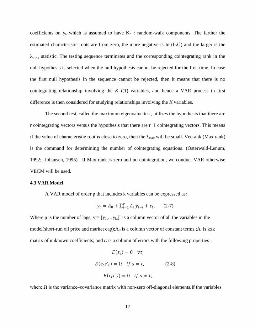
43 VAR Model
A VAR model of order p that includes k variables can be expressed as
119910119905 = 1198600 + 119860119894119875119894=1 119910119905minus119894 + 휀119905 (2-7)
Where p is the number of lags yt= [y1thellipykt]` is a column vector of all the variables in the
model(short-run oil price and market cap)A0 is a column vector of constant terms Ai is kxk
matrix of unknown coefficients and εt is a column of errors with the following properties
119864 휀119905 = 0 forall119905
119864 휀119905휀`119905 = Ω 119894119891 119904 = 119905 (2-8)
119864 휀119905휀`119905 = 0 119894119891 119904 ne 119905
where Ω is the variancendashcovariance matrix with non-zero off-diagonal elementsIf the variables
18
considered in this study are not cointegrated then the unrestricted VAR is used
If the variables are cointegrated and I(1) a vector error correction model can be employed This
method of analysis permits us to test for the direction of causality cointegration analysis is
conducted to shed light on the long-run relations that may exist among the series of nine ME
economies Following Johansen (1995) Harris and Sollis (2003) Lutkepohl (2005) Miller and
Ratti (2009) Greene (2007) and Nwosa (2014) we estimated VECM for series cointegrated
with OP and VAR for series which are not cointegrated with OP
To investigate whether oil price shocks influence ME stock market capitalization we
utilized a restricted VAR which is VECM and unrestricted VAR with a linear specification of oil
price and stock market capitalization The error terms were assumed to be zero-mean
independent white noise processes Based on related literature (Cologni and Manera 2008
Apergis and Miller 2009 Filis and Chatziantoniou 2014) we constructed a VAR model to
examine the influence of oil prices on market capitalization
119872119862119894119905 = 120593 + 120572119894119872119862119905minus119894 + 120573119894
119901
119894=1
119901
119894=1
119874119875119905minus119894 + 휀119905 (2 minus 9)
Where MCit is the market capitalization for country i at time t and tOP is the average oil price at
time t 120593 is constant and 120572119894 120573119894 119894 = 1 hellip119901 denote the linear relationship between variables MCt
and OPt
We lagged the explanatory variables to account for past value influences on the MC
variable and to determine whether the dependent variable is predictable or not Indeed the
impact of oil prices on MC might not happen immediately in which case lagged explanatory
variables are appropriate To determine the optimal length of oil price impact it is important to
take into account the market capitalization of the previous year The optimal length of impact
19
was determined by using the AIC This criterion determines the maximized log-likelihood of the
model where k is the number of parameters estimated and the model with the lowest AIC is
utilized
The models of VAR and VECM are able to capture the dynamics of the interrelationships
between the variables Impulse response functions or IRFs measure the effects of oil price
shocks to stock market cap variable The IRF examines the response while the model shocked by
a one-standard-deviation Further the models are able to capture the dynamics of the
interrelationships between the variables The IRFs represents the dynamic response path of a
variable due to a one-period standard deviation shock on another variable Based on these
models the impact of oil price movement on stock market capitalization is examined using
generalized impulse response functions (IRFs)
5 Data and Descriptive Statistics
In this section we describe the variables and sample periods and provide an economic
overview of the sample countries Nine countries in the ME considered for the study are United
Arab Emirates (ARE) Bahrain (BHR) Egypt (EGY) Israel (ISR) Jordan (JOR) Kuwait
(KWT) Qatar (QAT) Saudi Arabia (SAU) and Turkey (TUR) Among these nine countries
Israel Jordan Egypt and Turkey are net importers while the remaining countries are oil
exporters Table 2-1 presents selected macroeconomic indicators for the ME economies The
percentage of stock market capitalization to GDP ranges from 167 in Egypt to 854 in
Kuwait which shows variation between countries in terms of market capitalization Saudi
Arabia is the top exporter of petroleum products in the world United Arab Emirates ranked in
the 6th position Kuwait ranked in the 13th and Qatar ranked in the 14th position In each of
these countries energy exports contributed the vast majority of total exports (TE) ranging from
20
87 to 94 Industrial and service sectors contributed more than 90 of the GDP for every
country in the ME region except for Egypt Finally oil rents contribute a significant portion of
GDP for some ME countries like Kuwait (53) and Saudi Arabia (387) while for others (like
Israel Jordan and Turkey) these percentages are zero or close to it
To analyze the impact of OP on nine ME stock markets we used daily data Instead of
analyzing stock returns we focus on the MC within each market where MC is defined as the
total tradable value of the number of outstanding shares times the share price Based upon results
from the Zivot-Andrews test attributed to expanded shale oil production and the global financial
crisis it was determined to split the data between two periods Thus while the dataset covers the
period from 2001 to 2015 and analyses were conducted for two sub-periods of 2001-2008 and
2009-2015
Historical data on outstanding shares and the share price for the selected ME stock
markets were obtained Compustat Global through the Wharton Research Data Services
(WRDS) We calculated MC for each company and merged for all companies for each country
Data were expressed in monetary units for local currencies and converted to US dollars The
data files were sorted by Global Company Key (GVKEY) which is a unique six-digit number
represented for each company (issue currency and index) in the Capital IQ Compustat
Database2 Given that there is a large amount of missing data before 2001 we selected daily data
after January 1th
2001
Oil price data were obtained from the US Energy Information Administration (EIA)
using the Brent oil spot price the benchmark price in the oil market measured in US dollars per
2 The raw data includes trading shares and prices of shares or closed day value of each share for every company in
the nine ME stock markets The share price of each company has a specific code Outstanding shares are traded not
always on a given day for each company in the ME stock markets GVKEY is a unique six-digit number key
assigned to each company (issue currency and index) in stock market within each country Market capitalization
values were created for each country by aggregating over GVKEYs
21
barrel Oil prices show fluctuating patterns occur over time particularly after 2008 Some events
creating these fluctuations include Venezuela cutting off oil sales to ExxonMobil in February
2008 production from Iraqi oil fields not recovering from wartime damage the US shale gas and
oil production boom and international sanctions against Iranlsquos oil-dominated economy These
events led rising oil prices from 2004 until the financial crisis in 2008 driven primarily by
surging demand and supply shocks in the oil market (Smith 2009) Then in 2009 oil prices fell
sharply due to a surplus of oil production and the US tight oil production OPEC the largest
player in the oil market in 2009 failed to reach an agreement on production curbs resulting in
plummeting prices
The two main variables are analyzed using natural logarithms for several reasons (1)
coefficients for variables on a natural-log scale are directly interpretable as proportional
differences and (2) following previous studies (Maghayereh and Al-Kandari 2007 Arouri et al
2012 Filis and Chatziantoniou 2014) we utilize logged data to examine the impacts of OP on
the MC (Maghayereh and Al-Kandari 2007 Arouri et al 2012) Thus logarithmically
transforming variables is a proper way to handle stock and oil market where there exists a non-
linear relationship exists between the oil prices and stock market capitalization In addition
logarithmic forms are a suitable way to transfer skewed variables to a log-normal distribution
form Results of skewness in Table 2-2 show that MC and OP are skewed and have asymmetric
distributions
Table 2-2 presents the descriptive statistics related to OP and MC Nominal mean oil
price between 2001 and 2015 was $6714 USD per barrel the minimum and maximum varied
between $175 USD and $1454 USD during the study period The degree of correlation between
MC and daily OP among the ME countries was strongly positive with all correlation coefficients
22
above 070 Saudi Arabia ranked highest in terms of mean MC at $311 billion USD followed by
UAE at $121 billion USD and Kuwait with $111 billion USD
Figure 22 presents charts of oil prices and market capitalization by country Oil prices
show fluctuating patterns over time and are particularly volatile after 2008 Some events creating
these fluctuations include Venezuela cutting off oil sales to ExxonMobil in February 2008
production from Iraqi oil fields not recovering from wartime damage the US shale gas and oil
production boom starting around 2008 and international sanctions against Iranlsquos oil-dominated
economy Oil prices rose consistently from 2004 until the financial crisis in 2008 driven
primarily by surging demand and supply shocks in the oil market (Smith 2009) Then in 2009
oil prices fell sharply due to a surplus of oil production in the US and around the world OPEC
the largest player in the oil market in 2009 failed to reach an agreement on production curbs
resulting in plummeting prices For market capitalization these data show dramatic changes
from 2001 through 2005 for the stock markets in SAU ARE and BHR While showing a general
upward trend the other six countries donlsquot show such large changes in MC during the early time
periods
6 Results and Discussion
For each selected country we tested for unit roots to check for stationary in OP and MC
variables We estimated ADF and PP unit root tests for each of the variables and their first
differences These tests were based on null hypotheses of unit root for all variables Values from
ADF and PP show that MC and OP variables were non-stationary at level since the null
hypothesis of unit root could not be rejected for most of the countries particularly for OP (Table
2-3) Therefore the first difference of each series was taken and both the ADF and the PP test
statistics were once again computed with these first difference values The null hypothesis of the
23
unit root test was rejected when their first differences were considered Based on Table 2-3
results it was concluded that both OP and MC are integrated by an order of one I(1) ie
stationary at first difference for all nine economies and therefore suitable to investigate the
presence of a long-run relationship between these two variables
Moreover the Zivot-Andrews (ZA) test was added to ADF and PP tests for stationarity in
order to take into consideration structural breaks that can occur in the intercept andor the trend
of a data series (Zivot and Andrews 1992) The results of the ZA unit root test with trend are
summarized in Table 2-3 Crude oil prices were non-stationary and the MC variables were non-
stationary in every country except for Bahrain Jordan and Qatar - which were stationary in
level However both variables were stationary in first differences for all nine countries
By country the break dates from the ZA tests were consistent between series The ZA
test results of oil price show that the day of the structural break was Oct 22 2007 However the
date of December 31 2008 was utilized as the date for splitting the OP and MC data in order to
correspond with the financial crisis an in 2008 and shale oil revolution Thus the influence of
shale oil production and global financial crisis conditions are measured by dividing the sample
period into two balanced sub-periods pre-shale (20001-2008) and post-shale (2009-2015) For
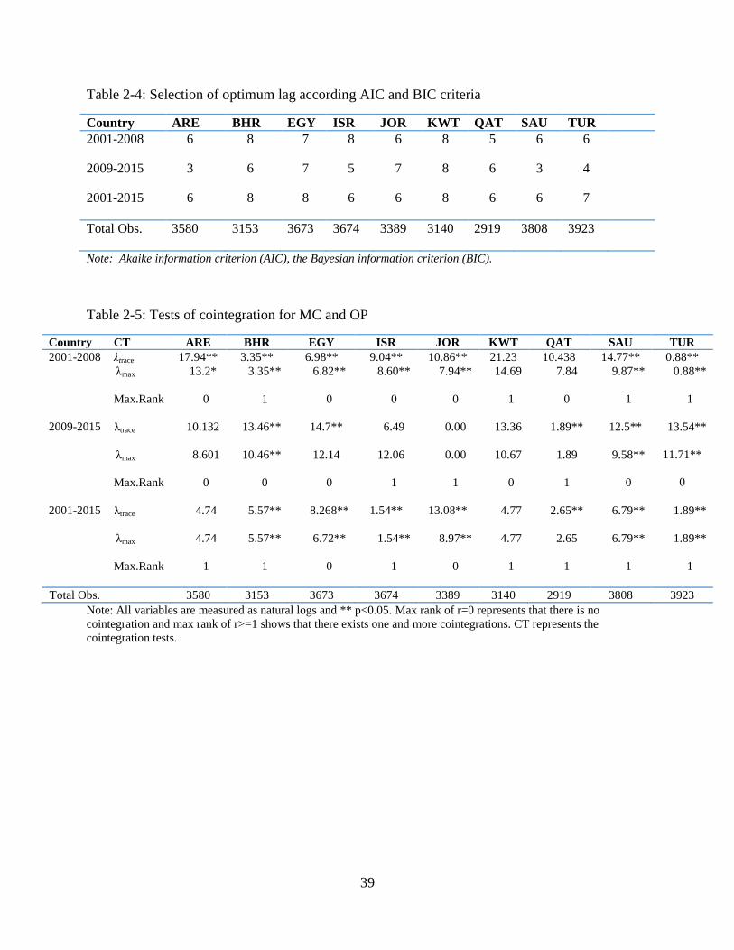
each period the lag length is selected according to the Akaike information criterion (AIC) Table
2-4 shows that the optimum lengths of lags for the two variables for each country in different
time periods (2001-2008 2009-2015 and 2001-2015) United Arab Emirates (636) Bahrain
(868) Egypt (778) Israel (856) Jordan (676) Kuwait (888) Qatar (566) Saudi Arabia
(636) and Turkey (647)
After confirming that all the variables contain a unit root we examine whether
cointegration changed significantly across the three periods This stage involves testing for the
24
existence of a long-run equilibrium linkage between OP and MC using Johansenlsquos cointegration
test Results for both the trace and maximum eigenvalue tests are reported in Table 2-5 Based on
the cointegration test long-run linkages for MC and OP differ for in all nine countries during the
three periods 2001ndash2008 2009-2015 and 2001ndash2015 The value of the λtrace test statistic and
eigenvalue λmax in the period 2001-2008 show that there exists cointegration for BHR KWT
SAU and TUR Hence the null hypotheses of no-cointegration (r = 0) are rejected in favor of a
co-integrating relationship between the OP and MC variables Conversely there are no-
cointegration and long-run linkages between MC and OP for ARE EGY JOR ISR and QAT in
that time period During the 2009-2015 there are cointegration relationships in ME stock
markets of ISR JOR and QAT and no cointegration in the remaining countries The existence
of a cointegrating relationship among OP and MC suggests that there is causality in at least one
direction however it does not determine the direction of causality between the variables
Bahrain Saudi Arabia Kuwait and Turkey have cointegration relationships in the period
of 2001-2008 After the global financial crisis our results indicate that only ISR JOR and QAT
have cointegration relationship We can argue that the global financial crisis affected all oil-
exporting countries except Qatar during the second period of the study These results are
possibly related to reforms in the Qatar economy and financial markets since the Qatar
government has been making efforts to diversify its economy away from crude oil income
In 2008 natural gas overtook crude oil as the largest contributor to the economy of Qatar
Crude oil and natural gas together accounted for 462 percent of the overall GDP of Qatar
(2009) for the first time overtaken by non-oil and gas sectors in the Qatari Markets Performance
Indicators of the Financial Sector didnlsquot change in Qatar prior to the end of 2008 It also resulted
in an accumulation of non-oil sectors and foreign assets In fact Qatars stock market has not
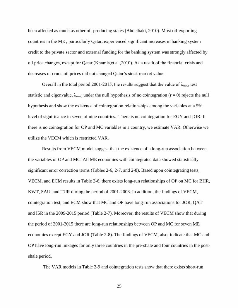
25
been affected as much as other oil-producing states (Abdelbaki 2010) Most oil-exporting
countries in the ME particularly Qatar experienced significant increases in banking system
credit to the private sector and external funding for the banking system was strongly affected by
oil price changes except for Qatar (Khamisetal2010) As a result of the financial crisis and
decreases of crude oil prices did not changed Qatarlsquos stock market value
Overall in the total period 2001-2015 the results suggest that the value of λtrace test
statistic and eigenvalue λmax under the null hypothesis of no cointegration (r = 0) rejects the null
hypothesis and show the existence of cointegration relationships among the variables at a 5
level of significance in seven of nine countries There is no cointegration for EGY and JOR If
there is no cointegration for OP and MC variables in a country we estimate VAR Otherwise we
utilize the VECM which is restricted VAR
Results from VECM model suggest that the existence of a long-run association between
the variables of OP and MC All ME economies with cointegrated data showed statistically
significant error correction terms (Tables 2-6 2-7 and 2-8) Based upon cointegrating tests
VECM and ECM results in Table 2-6 there exists long-run relationships of OP on MC for BHR
KWT SAU and TUR during the period of 2001-2008 In addition the findings of VECM
cointegration test and ECM show that MC and OP have long-run associations for JOR QAT
and ISR in the 2009-2015 period (Table 2-7) Moreover the results of VECM show that during
the period of 2001-2015 there are long-run relationships between OP and MC for seven ME
economies except EGY and JOR (Table 2-8) The findings of VECM also indicate that MC and
OP have long-run linkages for only three countries in the pre-shale and four countries in the post-
shale period
The VAR models in Table 2-9 and cointegration tests show that there exists short-run
26
causality running from OP to MC for ARE EGY ISR JOR and QAT in the 2001-2008 period
Moreover cointgration tests and VAR results in Table 2-10 provide evidence that there exists
short-run linkages for ARE BHR EGY KWT and SAU but not TUR in the 2009-2015 In
comparison there are five economies with shortndashrun and four countries with long-run linkages
between OP and MC in the 2001-2008 In the 2001-2015 period EGY and JOR are the only
countries where OP and MC were not cointegrated Thus we applied the unrestricted VAR
model (Table 2-11) The results of the unrestricted VAR model provide evidence that there is a
short-run causality running from OP to MC in these two economies
The ME stock markets consist of a variety of business and economic sectors Firms and
stock markets in oil exporting have more reliance on oil income While the stock market of
United Arab Emirates has been diversifying in different categories including financial and
banking insurance industrial sector and energy companies its economy remains extremely
reliant on crude oil as more than 85 of the United Arab Emirateslsquo economy was based on the
oil exports in 2009 In Bahrain listed companies in stock market are mostly in banking
insurance and financial sector As an oil-exporter Bahrain depends upon oil revenue and
shareholderslsquo investment relies on money and salaries from oil prices In the Saudi Arabia stock
market listed companies include energy materials capital goods transportation commercial
and professional services insurance banking and health care Likewise the stock markets in
Kuwait and Qatar consist of energy industrial financial insurance and commercial services In
the Egyptian stock market there are more diversified business and companies in industrial
energy health care financial tourism and hotels The results imply that most oil-exporting
countries have affected by changing crude oil prices since the companies and shareholders are
more influenced by crude oil price changes when compared to oil-importing countries in the ME
27
Oil-importing countries such as Israel Jordan and Turkey have more non-petroleum
companies and less dependency on oil income in the stock market In Israel its stock market is
based on high tech companies energy sector real estate and industrial companies Jordanlsquos stock
market is based upon the performance 100 of the largest companies of financial industrial
services and tourism sectors These sectors represent around 90 percent of the aggregate market
capitalization of the listed companies in Jordan The Turkish stock market consists more of
companies from industrial and manufacturing agricultural real estate and commercial services
Finally we examine the effect of OP shocks on MC by examining the impulse response
functions (IRFs) The IRFs map out the response of a one standard deviation shock of OP or MC
to the shock in the error term in VAR system which include unrestricted VAR and VECM over
several time periods An IRF measures the effect of a shock to an endogenous variable on itself
or on another exogenous variable (Lutkepohl 2005) Based on these models the impact of OP
movement on MC is examined using cumulative IRFs Hence the IRF of the VAR and VEC
models enable us to examine how each of the variable responds to innovations from other
variables in the system The orthogonal innovations denoted by εt are obtained by the errors
terms in Equation (2-7) which indicate that error values are uncorrelated with each other Results
for nine countries and 95 confidence bounds around each orthogonalized impulse response
appear in Figure 2-2
We make three observations First we find a significant change in how MC reacts to
shocks in OP changes before versus after 2008 For the period of 2001-2008 the response of MC
to a shock in OP seems to be small and mainly increasing over time Second the IRF results in
the 2009-2015 period show that OP has negative impact on MC in ME economies except for
EGY JOR and KWT These negative effects are possibly due to some combination of the global
28
financial crisis and expanded shale oil production both of which seem to have affected the ME
economies Third the IRFs show that the responses of all nine stock markets to one standard
deviation crude oil price shock displays fluctuations with both positive and negative effects
7 Conclusions
In this paper we analyze whether or not crude oil price changes have dynamic long-run
associations with stock market capitalization in nine ME economies using daily data for the
period 2001ndash2015 by means of estimating multivariate VECM and VAR models In order to
estimate the effect of OP shocks on MC we include cointegration tests and IRFlsquos The inclusion
of these tools help us understand the linkages between OP and MC in the ME region
The empirical analyses provide some important characteristics of OP and MC for nine
ME economies in three different periods (Table 2-12) Among the nine countries considered in
this study OP and MC were cointegrated in each country except for EGY and JOR during the
entire time period of 2001-2015 This suggests that a dynamic long-run causality linkage exists
between the two variables of OP and MC Oil exporting countries (ARE BHR KWT QAT and
SAU) had long-run relationships while oil importing countries (EGY ISR JOR and TUR) had
short-run relationships The findings show that OP has statistically significant short and long
run effects on MC across all nine economies These results suggest that stock market
capitalization have reacted to the changes of crude oil prices in the oil-exporting which have
more dependency on oil prices and income from oil
Prior to the financial crisis and the shale oil revolution (2001-2008) the results show that
there existed long-run causality between OP on MC for BHR KWT SAU and TUR During
this time period VAR models show that there exists short-run causality running from OP to MC
for ARE EGY ISR JOR and QAT in the 2001-2008 period The empirical results show that
before the global financial crisis and expanded shale oil production crude oil prices increased
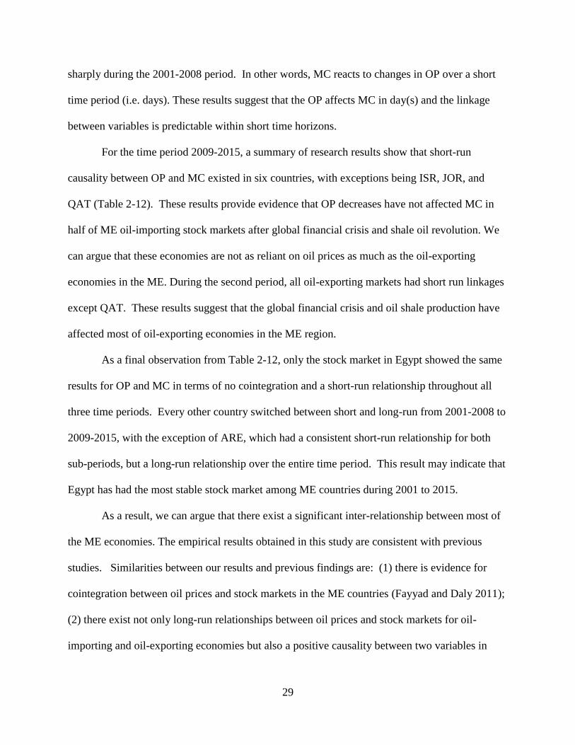
29
sharply during the 2001-2008 period In other words MC reacts to changes in OP over a short
time period (ie days) These results suggest that the OP affects MC in day(s) and the linkage
between variables is predictable within short time horizons
For the time period 2009-2015 a summary of research results show that short-run
causality between OP and MC existed in six countries with exceptions being ISR JOR and
QAT (Table 2-12) These results provide evidence that OP decreases have not affected MC in
half of ME oil-importing stock markets after global financial crisis and shale oil revolution We
can argue that these economies are not as reliant on oil prices as much as the oil-exporting
economies in the ME During the second period all oil-exporting markets had short run linkages
except QAT These results suggest that the global financial crisis and oil shale production have
affected most of oil-exporting economies in the ME region
As a final observation from Table 2-12 only the stock market in Egypt showed the same
results for OP and MC in terms of no cointegration and a short-run relationship throughout all
three time periods Every other country switched between short and long-run from 2001-2008 to
2009-2015 with the exception of ARE which had a consistent short-run relationship for both
sub-periods but a long-run relationship over the entire time period This result may indicate that
Egypt has had the most stable stock market among ME countries during 2001 to 2015
As a result we can argue that there exist a significant inter-relationship between most of
the ME economies The empirical results obtained in this study are consistent with previous
studies Similarities between our results and previous findings are (1) there is evidence for
cointegration between oil prices and stock markets in the ME countries (Fayyad and Daly 2011)
(2) there exist not only long-run relationships between oil prices and stock markets for oil-
importing and oil-exporting economies but also a positive causality between two variables in
30
majority of the ME stock markets (Filis et al 2011 Arouri and Roult 2012) (3) crude oil prices
could predict stock market capitalization in the ME economies (4) the IRFs of a response of MC
to OP shocks verify the positive relationship between oil prices and stock market value for most
of ME markets and (5) stock markets in both oil-importing and oil-exporting countries tend to
react to OP shocks either positive or negative(Yu et al 2008 Apergis and Miller 2009 Filis et
al 2011) These common findings prove a significant influence of OP on stock markets in the
region
In line with expectation most oil-exporting economies have positive short-run impacts of
OP on stock MC Among oil importing economies OP movement affects negatively on MC for
Israel Most of oil exporting economies considered in this study are heavily dependent on oil
price movements in particular in full sample Increase in oil price strengthens their economic
growth which in turn transmitted to higher MC These results suggest that a dynamic long run
causality among oil price and stock market capitalization for seven ME economies in total period
(Table 2-8)
This similarity of the findings for majority of ME economies can be explained by several
facts First since the ME countries having common land borders with each other they have close
economic relationships and increasing crude oil prices have impacts on the most economies
through increasing exports of goods and services from oil- importing to oil- exporting
economies Thus a higher crude oil price has benefits for both oil-importing and oil-exporting
countries in the region Since market capitalization determines the dynamic impact of oil price
changes it is argued that higher oil prices are needed to stimulate stock markets and economic
performance in the ME However consequences of this dependency in particular for oil-
exporting have had economic instability Since majority of oil-exporting rely on oil income oil
31
price shocks have affected their economies negatively Therefore a high priority for policy
makers in ME economies is to diversify their macro economies by improving the shares of the
non-oil industry and additional sectors to their economies
There are several limitations worth noting in this study First there is lack of available
and accurate data for all ME economies due to political instability in majority of countries
comparison to developed economies plus most of ME economies have thin markets for stocks
(Sowers et al 2011) While there are 17 counties in this region data could be obtained from
only nine economies In addition our research lacks considerations of how other
macroeconomic factors such as interest and exchange rates as well as future expectations for
cash flows may impact MC Future research could explore the influences of macroeconomic
activities and other factors contributing to the effect of oil prices on stock market activities in the
Middle Eastern economies such as interest rates shale oil production currency rates renewable
energy political instability and rates of conflict
32
8 References
Abhyankar A Xu B Wang J 2013 Oil price shocks and the stock market evidence from
Japan The Energy Journal 34(2) 199
Akaike H 1974 A new look at the statistical model identification IEEE Transactions in
Automatic Control 19(6) 716-723
Apergis N and Miller S M (2009) Do structural oil mdash market shocks affect stock prices
Energy Economics 31(4) 569minus575
Arouri M EH Roult C 2012 Oil prices and stock market in GCC countries empirical
Evidence from panel analysis International Journal for Finance and Economics 17(3)
242-253
Arouri M Jouini J Nguyen D 2011 Volatility spillovers between oil prices and stock sector
returns implications for portfolio management Journal of International Money and
Finance 301387-1405
Basher SA Sadorsky P 2006 Oil price risk and emerging stock markets Global Finance
Journal 17(2) 224-251
Brown SPA Yuumlcel MK 2002 Energy prices and aggregate economic activity an
interpretative survey Quarterly Review of Economics and Finance 42 193ndash208
Burbidge J Harrison A 1984 Testing for the Effects of Oil-Price Rises Using Vector
Autoregression International Economic Review 25 459-484
Chiou J Lee Y 2009 Jump dynamics and volatility oil and the stock markets Energy 34788-
96
Cologni A and Manera M 2008 Oil prices inflation and interest rates in a structural
cointegrated VAR model for the G-7 countries Energy economics 30(3) 856-888
Creane S Mobarak AM Goyal R and Sab R 2004 Financial sector development in the
Middle East and North Africa IMF Working Paper No 04201
Dickey D A Fuller W A 1981 Likelihood ratio statistics for autoregressive time series with
a unit root Econometrica Journal of the Econometric Society 49(4) 1057-1072
Dolado JJ Jenkinson T Sosvilla‐Rivero S 1990 Cointegration and unit roots Journal of
Economic Surveys 4(3) 249-273
Engle R F Granger C W 1987 Co-integration and error correction representation
estimation and testing Econometrica journal of the Econometric Society 251-276
33
Ewing BT Thompson MA 2007 Dynamic cyclical comovements of oil prices with
industrial production consumer prices unemployment and stock prices Energy Policy
35(11) 5535-5540
Ewing BT Malik F 2016 Volatility spillovers between oil prices and the stock market under
structural breaks Global Finance Journal 29 12-23
Fayyad A Daly K 2011 The impact of oil price shocks on stock market returns comparing
GCC countries with the UK and USA Emerging Markets Review 12(1) 61-78
Filis G Degiannakis S Floros C 2011 Dynamic correlation between stock market and oil
prices The case of oil-importing and oil-exporting countries International Review of
Financial Analysis 20(3) 152-164
Filis G and Chatziantoniou I 2014 Financial and monetary policy responses to oil price
shocks evidence from oil-importing and oil-exporting countries Review of Quantitative
Finance and Accounting 42(4) 709-729
Gadea MD Goacutemez-Loscos A and Montantildeeacutes A 2016 Oil price and economic growth a long
story Econometrics 4(4) 41
Ghalayini L 2011 The interaction between oil price and economic growth Middle Eastern
Finance and Economics 13 127-141
Global Database of Events Language and Tone (GDELT) 2016 All Information and Economic
indicators of Middle Eastern countries Retrieved from httpwwwgdeltprojectorg
Greene WH 2007 Econometric Analysis (7th
) New York University Prentice Hall
Le TH and Chang Y 2015 Effects of oil price shocks on the stock market performance Do
nature of shocks and economies matter Energy Economics 51 261-274
Hammoudeh S Aleisa E 2004 Dynamic relationships among GCC stock markets and
NYMEX oil futures Contemporary Economic Policy 22(2) 250-269
Harris R Sollis R 2003 Applied time series modelling and forecasting International Journal
of Forecasting 1 137-139
Henderson V 2003 The urbanization process and economic growth The so-what question
Journal of Economic growth 8(1) 47-71
Jimenez-Rodriguez R and Sanchez M 2005 Oil price shocks and real GDP growth empirical
evidence for some OECD countries Applied Economics 37(2) 201-228
Johansen S 1988 Statistical analysis of cointegration vectors Journal of EconomicDynamics
and Control 12(2-3) 231-254
34
Johansen S 1991 Estimation and hypothesis testing of cointegration vectors in Gaussian vector
autoregressive models Econometrica Journal of the Econometric Society 59(6) 1551-
1580
Johansen S 1992 Determination of cointegration rank in the presence of a linear trend Oxford
Bulletin of Economics and Statistics 54(3) 383-397
Johansen S 1995 Likelihood-Based Inference in Cointegrated Vector Autoregressive Models
Oxford University Press New York
Johansen S Juselius K 1990 Maximum likelihood estimation and inference on
cointegrationmdashwith applications to the demand for money Oxford Bulletin of
Economics and Statistics 52(2) 169-210
Jones DW Leiby PN Paik IK 2004 Oil price shocks and the macro economy what has
been learned since 1996 The Energy Journal 25(2) 1-32
Kilian L 2008 The economic effects of energy price shocks Journal of Economic
Literature 46(4) pp871-909
Lardic S Mignon V 2008 Oil prices and economic activity An asymmetric cointegration
approach Energy Economics 30(3) 847-855
Lardic S Mignon V 2006 The impact of oil prices on GDP in European countries An
empirical investigation based on asymmetric cointegration Energy policy 34(18) 3910-
3915
Lee K Ni S Ratti RA 1995 Oil shocks and the macroeconomy the role of price variability
The Energy Journal 16(4) 39-56
Lescaroux F Mignon V 2009 Measuring the Effects of Oil Prices on Chinalsquos Economy A
Factor‐Augmented Vector Autoregression Approach Pacific Economic Review 14(3)
410-425
Lutkepohl H 2005 New introduction to multiple time series analysis Econometric
Theory 22(5) 961-967
Maddala GS Wu S 1999 A comparative study of unit root tests with panel data and a new
simple test Oxford Bulletin of Economics and Statistics 61(S1) 631-652
Maghyereh A 2006 Oil price shocks and emerging stock markets A generalized VAR
approach In Global Stock Markets and Portfolio Management (55-68) Palgrave
Macmillan UK
Maghyereh A Al-Kandari A 2007 Oil prices and stock markets in GCC countries new
evidence from nonlinear cointegration analysis Managerial Finance 33(7) 449-460
35
Malik F Ewing BT Volatility transmission between oil prices and equity sector returns Int Rev
Finance Anal 2009 18(3) 95-100
Miller JI Ratti RA 2009 Crude oil and stock markets Stability instability and bubbles
Energy Economics 31(4) 559-568
Moon H R Perron B 2006 Seemingly unrelated regressions The New Palgrave Dictionary
of Economics 1-9
Nwosa PI 2014 Oil prices and stock market price in Nigeria OPEC Energy Review 38(1)
59-74
OPEC 2014 Organization for Petroleum Exporting Countries (OPEC) Retrieved from
httpwwwopecorg
Osterwald-Lenum M G 1992 A note with quantiles of the asymptotic distribution of the
maximum likelihood cointegration rank test statistics Oxford Bulletin of Economics and
Statistics 54 461ndash472
Park J Ratti RA 2008 Oil price shocks and stock markets in the US and 13 European
countries Energy Economics 30(5) 2587-2608
Phillips PCB Perron P 1988 Testing for a unit root in time series regression Biometrika
75 335-346
Piazza JA 2007 Draining the swamp Democracy promotion state failure and terrorism in 19
Middle Eastern countries Studies in Conflict amp Terrorism 30(6) 521-539
Sadorsky P 2006 Oil price risk and emerging stock markets Global Finance Journal 17(2)
224-251
Sadorsky P 1999 Oil price shocks and stock market activity Energy Economics 21(5) 449-
469
Selvik K Stenslie S 2011 Stability and Change in the Modern Middle East London IB
Tauris and Co Ltd
Smith JL 2009 The 2008 Oil Price Shock Markets or Mayhem Resources for the Future
Policy Commentary Series 6 Retrieved from httpwwwrfforgblog20092008-oil-
price-shock-markets-or-mayhem
Sowers J Vengosh A Weinthal E 2011 Climate change water resources and the politics of
adaptation in the Middle East and North Africa Climatic Change 104(3) 599-627
Temel B 2012 From Value to Power The Rise of Oil as a Political Economic Commodity
(No 201252) Discussion Paper Turkish Economic Association
36
Teulon F and Guesmi K 2014 Dynamic Spillover between the Oil and Stock Markets of
Emerging Oil-Exporting Countries Journal of Applied Business Research 30(1) 51
US Energy Information Administration 2016 Energy prices August 2016 Retrieved from
httpswwweiagovoutlookssteomarketreviewcrudecfm
World Bank 2015 World Bank open data Retrieved from httpdataworldbankorg
Yu J S Hassan M K 2008 Global and regional integration of the Middle East and North
African (MENA) stock markets The Quarterly Review of Economics and Finance 48(3)
482-504
Zellner A 1962 An efficient method of estimating seemingly unrelated regressions and tests
for aggregation bias Journal of the American Statistical Association 57(298) 348-368
Zivot E Andrews DWK 2002 Further evidence on the great crash the oil-price shock and
the unit-root hypothesis Journal of Business amp Economic Statistics 20(1) 25-44
37
Tables and Figures Table 2-1 Macroeconomic overview of ME region
ARE BHR EGY ISR JOR KWT QAT SAU TUR
Stock market
capitalization of listed
domestic companies ( of
GDP)
529 597 167 824 678 567 854 652 263
Energy exports ( of TE) 90 45 24 1 62 94 88 87 4
Oil exports global rank 6 33 40 0 0 13 14 1 0
Composition of GDP
Agriculture 0019 03 143 25 001 04 01 23 81
Industry 648 353 396 273 066 594 588 469 277
Service 033 644 461 70 033 402 411 508 642
GDP per Capita (USD) 42000 21200 6000 31000 5300 40700 102900 20400 16067
Oil rents as a ( of GDP) 216 153 58 0 0 53 195 387 02
Note the sources of some data in the table retrieve from US EIA (2016) World Bank (2015)
Table 2-2 Descriptive statistics for MC (billion USD) and for OP (USD per barrel)
MC ARE BHR EGY ISR JOR KWT QAT SAU TUR Oil
price
Mean 121 229 61 132 245 111 107 311 177 6714
Min 0 0 0 0 374 0255 276 0 0 175
Max 273 553 175 236 586 225 231 796 376 14531
SD
Skewness
754
0089
911
0 29
405
-0109
575
-012
115
-021
452
-0078
546
-003
176
-017
103
0011
2798
0012
Correlation with oil 072 07194 084 084 076 076 0701 072 083 -
Observations 3580 3153 3673 3674 3389 3140 2919 3808 3923
38
Table 2-3 Tests for unit root hypothesis for market capitalization and oil price
Country
Variables
Variables in level Variables in first
difference
Minimum
t-statistics3
ADF PP ADF PP ZA test
ARE
LMC -5134 -4779 -64889 -63914 -1885
LOP -1295 -1882 -62607 -62667 -2696
BHR
LMC -10627 -5504 -70095 -71261 -8475
LOP -1414 -1874 -97672 -57663 -2665
EGY
LMC -2005 -1395 -35094 -31572 -3384
LOP -1916 -1844 -64657 -64789 -2916
ISR
LMC -2005 -1395 -35094 -31572 -1140
LOP -1916 -1844 -64657 -64789 -2960
JOR
LMC -2561 -2419 -55905 -56004 -5129
LOP -1983 -1906 -62182 -62597 -2736
KWT
LMC -13082 -12831 -47985 -48028 -3386
LOP -2055 -1989 -56156 -56252 -2553
QAT
LMC -5380 -4971 -55234 -54962 -471
LOP -2317 -2252 -57234 -57458 -2836
SAU
LMC -1712 -4695 -60218 -60235 -3423
LOP -3842 -3796 -63890 -63987 -2906
TUR
LMC -1648 -1140 -78339 -81653 -2916
LOP -1892 -1817 -64755 -64883 -2916
Notes All variables are measured as natural logs and plt001 and z(t)= -3430 plt005 and z(t)= -2860
plt01 and z(t)= -2570 Critical values for ZA test 1(-493) 5(-442) and 10(-411) Based on Zivot-
Andrews unit test root tests for market capitalization and oil price in all economies except BHR JOR and QAT are
non-stationary in level while all countries are stationary in the first difference at 5 significance
3 The oil price break date is Oct 22 2007
39
Table 2-4 Selection of optimum lag according AIC and BIC criteria
Country ARE BHR EGY ISR JOR KWT QAT SAU TUR
2001-2008 6 8 7 8 6 8 5 6 6
2009-2015 3 6 7 5 7 8 6 3 4
2001-2015 6 8 8 6 6 8 6 6 7
Total Obs 3580 3153 3673 3674 3389 3140 2919 3808 3923
Note Akaike information criterion (AIC) the Bayesian information criterion (BIC)
Table 2-5 Tests of cointegration for MC and OP
Country CT ARE BHR EGY ISR JOR KWT QAT SAU TUR
2001-2008 λtrace 1794 335 698 904 1086 2123 10438 1477 088
λmax
MaxRank
132
0
335
1
682
0
860
0
794
0
1469
1
784
0
987
1
088
1
2009-2015
λtrace
λmax
MaxRank
10132
8601
0
1346
1046
0
147
1214
0
649
1206
1
000
000
1
1336
1067
0
189
189
1
125
958
0
1354
1171
0
2001-2015 λtrace 474 557 8268 154 1308 477 265 679 189
λmax
MaxRank
474
1
557
1
672
0
154
1
897
0
477
1
265
1
679
1
189
1
Total Obs 3580 3153 3673 3674 3389 3140 2919 3808 3923
Note All variables are measured as natural logs and plt005 Max rank of r=0 represents that there is no
cointegration and max rank of rgt=1 shows that there exists one and more cointegrations CT represents the
cointegration tests
40
Table 2-6 The result of VECM for MC and OP 2001-2008
Country BHR KWT SAU TUR
ECM(-1) -031(004) -003(00) -003(001) -02 (003)
ΔInMC(-1) -22( 025) -075(03) 014(02) -235(022)
ΔInMC(-2) -054( 026) 035(03) 008(02) -128(023)
ΔInMC(-3) -078(025) -021(03) 007(02) -025(023)
ΔInMC(-4) -04246(025) 023(03) 005(02) -041(023)
ΔInMC(-5) 21(03) 036(03) -005(02) -073(023)
ΔInMC(-6) -0705(026) -043(03) -006(02) -0065(022)
ΔInMC(-7) -062(025) -053(03)
ΔInMC(-8) -0312(025) 023(03)
ΔInMC(-9)
ΔInOP(-1) lrm0131(15) 031(015) -149(07) 036(041)
ΔInOP(-2) 0050(15) 017(015) 09(07) 003(041)
ΔInOP(-3) 1660(15) 013(015) 018(07) -001(041)
ΔInOP(-4) 0085(15) -014(015) -44(07) 043(042)
ΔInOP(-5) 0458(15) 035(015) -129(07) 037(042)
ΔInOP(-6) 1693(15) 008(015) -053(07) -045(042)
ΔInOP(-7) 821( 15) -0009(015)
ΔInOP(-8) 697(16) 018(015)
Obs 1476 1463 1998 1998
Note Standard errors are in parentheses significant at the 5 level
41
Table 2-7 The result of VECM for MC and OP 2009-2015
Country ISR JOR QAT
ECM(-1) -005(001) -004(001) -005(001)
ΔInMC(-1) -034(024) 06(02) -0378(024)
ΔInMC(-2) -001(025) -0301(02) 0285(024)
ΔInMC(-3) -11(024) 061(02) 0395(025)
ΔInMC(-4) 002(025) -050(02) -0015(025)
ΔInMC(-5) 034(025) -035(02) -0190(024)
ΔInMC(-6) -002(02) 0165(024)
ΔInMC(-7) 016(02)
ΔInMC(-8)
ΔInMC(-9)
ΔInOP(-1) -03(014) 039(008) 1239(015)
ΔInOP(-2) 018(014) 015(008) 0343(016)
ΔInOP(-3) 012(014) 004(008) 0533(016)
ΔInOP(-4) 012(014) -003(008) 0237(016)
ΔInOP(-5) 02(014) 031(008) 057(015)
ΔInOP(-6) 025(008) 0035(016)
ΔInOP(-7) -004(008)
ΔInOP(-8)
Obs 1672 1669 1654
Note Standard errors are in parentheses significant at the 5 level
42
Table 2-8 The result of VECM for MC and OP 2001-2015
Country ARE BHR ISR KWT QAT SAU TUR
ECM(-1) -002( 00) -001( 00) -03(001) -002(00) -001(00) -003(00) -001(00)
ΔInMC(-1) 0134(016) -80(01) -006(01) -03( 02) 062(02) 0169(016) -206(02)
ΔInMC(-2) 148( 016) -62(02) -018(015) -03( 02) 019(02) 0089(016) -101(02)
ΔInMC(-3) -0020(016) -49(021) -009 (015) -016(02) 027(02) 006(016) -007(017)
ΔInMC(-4) -0267(016) -43(023) 01(015) 013(02) 009(02) 003(016) -027(017)
ΔInMC(-5) 021(016) 22(024) -003(015) 036(02) -020(02) -005(02) -06(02)
ΔInMC(-6) -0096(015) 06(023) -006(013) -02(02) 004(01) -007(016) -001(016)
ΔInMC(-7) -038(021) -05(02)
ΔInMC(-8) -114(01) 027( 01)
ΔInMC(-9)
ΔInOP(-1) 055( 015) 099(04) -04( 02) 036(009) 077(01) 118(042) 036 (025)
ΔInOP(-2) 019(016) 150(041) -003(016) 02(009) 050(01) 091(042) 027 (025)
ΔInOP(-3) 033(016) 153(041) 04(08) 02(009) 045(01) 0199(042) 015 (025)
ΔInOP(-4) 0098(016) 055(041) 003(016) 02(009) 025(01) 265(043) 038 (025)
ΔInOP(-5) -0010(016) 172(041) -05(016) -00(009) 022(01) -068(043) 031 (025)
ΔInOP(-6) -0055(015) -052(041) -02(02) -004(009) 006(01) -028(043) -031 (025)
ΔInOP(-7) 015(041) 011(009)
ΔInOP(-8) -007(041) 024(009)
Obs 3580 3153 3674 3140 2919 3808 3923
Note Standard errors are in parentheses significant at the 5 level
43
Table 2-9 The result of VAR for MC and OP 2001-2008
Country ARE EGY ISR JOR QAT
ΔInMC(-1) 101(02) 15( 02) 43( 02) 11(02) 109(03)
ΔInMC(-2) 15(032) 158(02) 25( 02) -05 (035) -086( 04)
ΔInMC(-3) -17(032) 065(01) 09( 02) 03(035) 018( 04)
ΔInMC(-4) -037(033) 14(016) 15( 02) -03(035) -021(039)
ΔInMC(-5) 0482(030) 69(02) -006( 02) 007(035) -005(024)
ΔInMC(-6) -0134(020) -12( 02) -008( 02) -01(035)
ΔInMC(-7) -08( 02) -013( 02)
ΔInMC(-8) 09( 02)
ΔInMC(-9)
ΔInOP(-1) 045( 026) 16( 06) 05(03) 04(01) 052(025)
ΔInOP(-2) -0412(036) -01(09) -00(04) -03(017) 0221(034)
ΔInOP(-3) 03745(037) 07(09) 003(04) 008(017) -029(035)
ΔInOP(-4) -0223(036) -17(09) -007(04) -01(017) -005(035)
ΔInOP(-5) -0458(036) 13(09) -07(04) 005(017) -043(026)
ΔInOP(-6) 0260(026) -27(09) 03(04) -01(017)
ΔInOP(-7) 102(06) 06(04)
ΔInOP(-8) -06(03)
ΔInOP(-9)
Obs 1903 1996 1996 1711 1258
Note Standard errors are in parentheses significant at the 5 level
44
Table 2-10 The result of VAR for MC and OP 2009-2015
Country ARE BHR EGY KWT SAU TUR
ΔInMC(-1) 105(
024)
54(02) 50(02) 107(02) 102(02) 966( 025)
ΔInMC(-2) 0427(035) 13(02) 22(02) -09(03) 0024(03) 053(035)
ΔInMC(-3) -0940( 024) 18(02) 015(02) 01(035) -027(02) 028(035)
ΔInMC(-4) -047(02) 12(02) -03(035) -055( 025)
ΔInMC(-5) 51(02) 54(02) 06(035)
ΔInMC(-6) -34(02) -35(02) 019(035)
ΔInMC(-7) -06(02) -12(035)
ΔInMC(-8) 07(02)
ΔInMC(-9)
ΔInOP(-1) 0719( 012) -028(03) 016(03) 048(011) 065(01) 003(022)
ΔInOP(-2) -0374( 017) 11(04) 08(04) -017(015) 006 (02) 040(030)
ΔInOP(-3) -0329( 012) -0003(03) 014(04) 002(015) -07(01) -022(030)
ΔInOP(-4) -035(04) 014(05) -001(015) -018 (022)
ΔInOP(-5) -036(04) -056(04) -012(015)
ΔInOP(-6) -009(03) -13(04) -031(015)
ΔInOP(-7) 06(03) 05(015)
ΔInOP(-8) -034(011)
ΔInOP(-9)
Obs 1677 1669 1670 1669 1669 1669
Note Standard errors are in parentheses significant at the 5 level
45
Table 2-11 The result of VAR for MC and OP 2001-2015
Country EGY JOR
ΔInMC(-1) 19( 01) 106(016)
ΔInMC(-2) 17(02) -065(024)
ΔInMC(-3) 11(02) 046(024)
ΔInMC(-4) 14(01) -052(024)
ΔInMC(-5) 67(01) 013(024)
ΔInMC(-6) -15(02) -005(024)
ΔInMC(-7) -08(02)
ΔInMC(-8) -05(02)
ΔInMC(-9)
ΔInOP(-1) 11( 04) 035(007)
ΔInOP(-2) 0489(06) -025(010)
ΔInOP(-3) 0167 003(010)
ΔInOP(-4) -11(06) -012(010)
ΔInOP(-5) 10(06) 014(010)
ΔInOP(-6) -23(06) -015(007)
ΔInOP(-7) 07(06)
ΔInOP(-8) -004(06)
ΔInOP(-9)
Obs 3673 3389
Note Standard errors are in parentheses significant at the 5 level
46
Table 2-12 Summary of results
Period 2001-2008 2009-2015 2001-2015
Country r Linkage r Linkage r Linkage
United Arab Emirates(ARE) No SRR Yes SRR Yes LRR
Bahrain (BHR) Yes LRR No SRR Yes LRR
Egypt (EGY) No SRR No SRR No SRR
Israel (ISR) No SRR Yes LRR Yes SRR
Jordan (JOR) No SRR Yes LRR No SRR
Kuwait (KWT) Yes LRR No SRR Yes LRR
Qatar (QAT) No SRR Yes LRR Yes LRR
Saudi Arabia (SAU) Yes LRR No SRR Yes LRR
Turkey (TUR) Yes LRR No SRR Yes SRR
Note Cointegration (Yes rgt=1) no-Cointegration (No r=0 ) ECM (Long-run linkage LRR)
and VAR (Shortndashrun linkage SRR)
47
Figure 2-2 Market capitalization (MC in Billion USD) and crude oil price (OP in USD) by
Country
The United Arab Emirates (ARE)
050
100
150
OP
0
100
200
300
MC
Jan 01 2000 Jan 01 2005 Jan 01 2010 Jan 01 2015Date
MC OP
Bahrain (BHR)
050
100
150
OP
0
2000
040
000
6000
0
MC
Jan 1 2002 Jul 1 2006 Jan 1 2011 Jul 1 2015Date
MC OP
050
100
150
OP
050
100
150
200
MC
Jan 01 2000 Jan 01 2005 Jan 01 2010 Jan 01 2015Date
MC OP
Egypt (EGY) Israel (ISR)
050
100
150
OP
5010
015
020
025
0M
CS
Jan 01 2000 Jan 01 2005 Jan 01 2010 Jan 01 2015Date
MCS OP
050
100
150
OP
020
4060
MC
Jan 01 2000 Jan 01 2005 Jan 01 2010 Jan 01 2015Date
MC OP
Jordan (JOR)
050
100
150
OP
050
100
150
200
250
MC
Jan 01 2000 Jan 01 2005 Jan 01 2010 Jan 01 2015Date
MC OP
Kuwait (KWT)
050
100
150
OP
050
100
150
200
250
MC
Jan 01 2002 Jul 01 2006 Jan 01 2011 Jul 01 2015Date
MC OP
Qatar (QAT)Saudi Arabia (SAU)
050
100
150
OP
0
200
400
600
800
MC
S
Jul 01 2001 Jan 01 2005 Jul 01 2008 Jan 01 2012 Jul 01 2015Date
MC OP
48
Figure2-3 Impulse response function (IRF) for each Middle East econmy
ARE 2001-2008 2009-2015 2001-2015
BHR
050
100
150
OP
0
100
200
300
400
MC
Jan 01 2000 Jan 01 2005 Jan 01 2010 Jan 01 2015Date
MC OP
Turkey (TUR)
-1
0
1
2
0 5 10 15 20
var LMC LOP
95 CI impulse-response function (irf)
LM
C
LOP
Graphs by irfname impulse variable and response variable
-3
-2
-1
0
1
0 5 10 15 20
var LMC LOP
95 CI impulse-response function (irf)
LM
C
LOP
Graphs by irfname impulse variable and response variable
-02
-01
0
01
02
0 5 10 15 20
order1 LMC LOP
95 CI
LM
C
LOPGraphs by irfname impulse variable and response variable
0
005
01
015
0 5 10 15 20
vecm LMC LOP
95 CI
LM
C
LOPGraphs by irfname impulse variable and response variable
-015
-01
-005
0
005
0 5 10 15 20
vecm LMC LOP
95 CI
LM
C
LOPGraphs by irfname impulse variable and response variable
49
EGY
ISR
JOR
-04
-02
0
02
04
0 5 10 15 20
var LMC LOP
95 CI impulse-response function (irf)
LM
C
LOP
Graphs by irfname impulse variable and response variable
-04
-02
0
02
04
0 5 10 15 20
var LMC LOP
95 CI impulse-response function (irf)
LM
C
LOP
Graphs by irfname impulse variable and response variable
-04
-02
0
02
0 5 10 15 20
var LMC LOP
95 CI impulse-response function (irf)
LM
C
LOP
Graphs by irfname impulse variable and response variable
-05
0
05
1
0 5 10 15 20
var LMC LOP
95 CI impulse-response function (irf)
LM
C
LOP
Graphs by irfname impulse variable and response variable
-2
-15
-1
-05
0
0 5 10 15 20
vecm LMC LOP
95 CI
LM
C
LOPGraphs by irfname impulse variable and response variable
-02
-01
0
01
02
0 5 10 15 20
vecm LMC LOP
95 CI
LM
C
LOPGraphs by irfname impulse variable and response variable
-2
-1
0
1
2
0 5 10 15 20
var LMC LOP
95 CI impulse-response function (irf)
step
Graphs by irfname impulse variable and response variable JOR2001-2008
-1
-05
0
05
0 5 10 15 20
vec LMC LOP
stepGraphs by irfname impulse variable and response variable JOR2009-2015
-3
-2
-1
0
1
0 5 10 15 20
var LMC LOP
95 CI impulse-response function (irf)
step
Graphs by irfname impulse variable and response variableJOR2001-2015
50
KWT
QAT
SAU
-1
-05
0
05
0 5 10 15 20
vecm LMC LOP
95 CI
LM
C
LOPGraphs by irfname impulse variable and response variable
-4
-2
0
2
4
0 5 10 15 20
var LMC LOP
95 CI impulse-response function (irf)
LM
CLOP
Graphs by irfname impulse variable and response variable
-1
-05
0
05
0 5 10 15 20
vecm LMC LOP
95 CI
LM
C
LOPGraphs by irfname impulse variable and response variable
-1
0
1
2
0 5 10 15 20
var LMC LOP
95 CI impulse-response function (irf)
LM
C
LOP
Graphs by irfname impulse variable and response variable
-4
-2
0
0 5 10 15 20
vecm LMC LOP
95 CI
LM
C
LOPGraphs by irfname impulse variable and response variable
-04
-02
0
02
0 5 10 15 20
vecm LMC LOP
95 CI
LM
C
LOPGraphs by irfname impulse variable and response variable
-015
-01
-005
0
0 5 10 15 20
vecm LMC LOP
95 CI
LM
C
LOPGraphs by irfname impulse variable and response variable
-4
-3
-2
-1
0
0 5 10 15 20
var LMC LOP
95 CI impulse-response function (irf)
LM
C
LOP
Graphs by irfname impulse variable and response variable
-02
-015
-01
-005
0
0 5 10 15 20
vecm LMC LOP
95 CI
LM
C
LOPGraphs by irfname impulse variable and response variable
51
TUR
0
05
1
0 5 10 15 20
vecm LMC LOP
95 CI
LM
C
LOPGraphs by irfname impulse variable and response variable
-3
-2
-1
0
1
0 5 10 15 20
var LMC LOP
95 CI impulse-response function (irf)
LM
C
LOP
Graphs by irfname impulse variable and response variable
-01
0
01
02
03
0 5 10 15 20
vecm LMC LOP
95 CI
LM
C
LOPGraphs by irfname impulse variable and response variable
52
Chapter 3 - Essay 2 The Dynamic Response of Coal Consumption to Energy Prices and
GDP An ARDL Approach to the US
1 Introduction
A variety of energy sources and technologies are used in the United States to generate
electricity These sources and technologies have changed over time based upon price efficiency
and environmental impacts The US Energy Information Administration (EIA) lists the three
main categories of energy sources for the 4015 billion kilowatt-hours (kWh) of electricity
generated in 2017 fossil fuels (coal natural gas and petroleum) nuclear energy and renewable
energy sources About 63 of this electricity generation is from fossil fuels (coal natural gas
petroleum and other gases) of which just under frac12 of this power supply originates from coal
Coal has served as a crucial source of energy to generate electricity for many decades As much
of the US gravitates towards more efficient and sustainable energy sources for generating
electricity natural gas is seen as a transition fossil fuel able to produce less polluting electricity
than coal The possibility for substitution between energy sources and the sensitivity of power
utilities to changes in the prices of energy sources are essential for understanding energy markets
as policy makers seek to promote cleaner energy and enhance energy efficiency Therefore coal-
to-natural gas substitution in the power plants is expected to drive consumption down for coal in
energy market
Rising concerns about climate change have resulted in increased consumption of clean
energy for electricity in the US as well as in nations around the world Fuel switching or the
substitution of low-carbon energy sources for fossil fuels with higher carbon content is one of the
principal methods suggested to reduce carbon dioxide (CO2) emissions (Hayhoe et al 2002)
53
According to the US EIA the amount of CO2 produced when coal (228)4 is burned is almost
twice that of natural gas (117) due to the carbon content of the coal Thus utilization of natural
gas in place of coal leads to a significant reduction in CO2 emissions when generating electricity
Natural gas is a possible alternative to coal also improves conversion efficiency of energy to
electricity 62 for natural gas (rising to over 90) compared to a 25 to 35 efficient coal-
fired plant (Audus 1999 Nakicenovic 2000 Hayhoe et al 2002) Considering that the
majority of CO2 emissions originate from coal consumption the ability to switch coal to natural
gas in the power plants become a main target and instrument for energy and environmental
policy makers
Furthermore choices of fuel and factor alternatives are critical issues in energy policy A
natural gas price shock could have significant impacts on the costs and utilization of coal in
energy market and power plant relatively (Atkeson and Kehoe 1999) Since natural gas
combustion has lower amounts of CO2 sulfur dioxide (SO2) nitrogen oxides (NOx) emissions
per megawatt hour (MWh) fuel displacing from coal to natural gas reduces environmental
emissions We could argue that increased natural gas usage by power plants is not only related to
efficiency and reducing pollution but also leads to enhanced links between natural gas and coal
prices
Natural gas development has increased gradually in the USlsquo energy industry Coal has
long been the US preferred source of cheaper energy although falling natural gas prices that
stabilized below $250MBTU make natural gas a competitive energy source for power plants
(Slingsby 2015) During the past three decades the natural gas market has seen significant price
volatility and the US energy market has shifted away from coal-fired power plants toward
natural gasndashfired power generation (US EIA 2016) Moreover the commercialization of
4Pounds of CO2 emitted per million British thermal units (Btu) of coal
54
fracking technology starting in the 2008-2009 led to dramatically lower natural gas prices At
the same time US electricity generation from coal has decreased along with domestic coal
consumption (Figure 3-1) As a result the production of coal has decreased over past two
decades As shown in Figure 3-2 decreasing coal extraction has affected labor market and
income for local and state economies in the most producing coal states in the US 5(EIA 2017)
Moreover efficiency and lower natural gas prices have led to more consumption of natural gas
and less production of coal due to the development of shale gas resources in the US (US EIA
2016)
Figure 3-1 US power generation from coal and natural gas (source US EIA (2016))
5 There are 11 states including Wyoming West Virginia Pennsylvania Illinois Kentucky Texas Montana Indiana
North Dakota Colorado and Ohio
55
Figure 3-2 Coal producing states and change in coal production (source US EIA (2017))
Fuel choice for power generation relies on fuel prices While the elasticity of demand for
energy as a whole is low (Platchkov and Pollitt 2011) own-price demand elasticity for coal
should be positive because of the presence of demand side substitutes for coal such as natural
gas and renewable energy sourves Thus there will be a shift from coal to natural gas if natural
gas prices remain lower compared to coal as both coal and natural gas are consumed in
electricity generation A study conducted by US EIA (2012) showed that coal consumption and
natural gas price cross elasticity was 017 and own price elasticity was -011 for coal If coal and
natural gas are substitutes it is hypothesized that there is a positive relationship between
consumption of coal and price of natural gas
The effects of natural gas prices on economic activities have been studied but the related
research have lesser insights for changes of natural gas price and related impacts on the coal
industry There is literature (Hamilton 2005 Kilian 2008) about the linkage between energy
prices and economic activity but there is no study specifically related to natural gas price
volatility and coal consumption Accordingly several studies using various estimation models
and samples have been applied to the analysis of energy elasticities and fuel substitution in
energy markets However no previous research has estimated the relationship between both coal
56
and natural gas prices and coal consumption in the US This study is the first research to
examine linkage between energy prices and the consumption of coal in the US energy market
using an Autoregresive Distributive Lag (ARDL) model The focus of this study is to investigate
the linkages between coal and natural gas prices and the coal consumption in the US and to
reveal other characteristics and underlying elements in the coal market
It is critical to examine the changing relationship between natural gas and coal since
natural gas has been expanding its electricity generation market share at the expense of coal in
recent years (Figure 3-1) Recent evidence shows that utilities are more likely to build natural
gasndashfired plants than coal-fired plants (US EIA 2012 Xie et al 2016) Given this background
the present research investigates both the long-run and short-run dynamic responses of coal
consumption in the US to changes in energy prices (coal and natural gas) along with GDP and
other related factors It is important to know the potential magnitude of impacts from price based
policies to determine their suitability for transitioning to clean energy sources thereby reducing
carbon emissions for the US economy
The main contribution of this study is to develop an economic framework for estimating
the dynamic longndashrun linkages between coal-natural gas prices and coal consumption in the US
economy In addition this research contributes to the literature by establishing coal-natural gas
linkages utilizing an ARDL model that allows for exploration of both short and long-run
relationships among variables A novel contribution is estimating how much of the decrease in
coal use occurred as a result of declining natural gas prices in the US energy market This
research investigates the extent to which coal and natural gas prices economic growth and other
factors have encouraged a switch from coal use to natural gas consumption If coal consumption
responds significantly to these factors these changes impact policy makers towards encouraging
57
alternative energy sources such as natural gas Hence to determine the strength of relationships
we examine the short and long-run correlations between coal consumption natural gas price
coal price and other factors over time period 2000-2016
The organization of the paper is as follows Section 2 gives a summary of previous
studies Sections 3 and 4 include discussions of the theoretical approach and empirical model
Section 5 presents the empirical results
2 Literature Review
In recent years the crisis of coal industry in the US has received increasing attention in
the literature The potential for natural gas to replace coal has promoted recommendation that
natural gas could be used as a bridging fuel until close to zero carbon energy sources are more
environmentally and economically viable (Levi 2013) Burke and Lioa (2015) found evidence
from provincial data in China that in the long- run coal demand has increasingly price elastic
Hence Chinalsquos coal market is more suitable for price based approach to reduce demand
The issue of energy demand and coal industry have also become the subject matter of
scholarly studies that address various topics For instance Apergis and Payne (2010) examine
the renewable and non-renewable energy demand finding that the demand of clean energy
sources increase with the growth of economy Nonetheless the relationship between economic
growth and energy consumption remain a debate (Hamilton 2005 and Kilian 2008 Apergis and
Payne 2012 Salim and Hassan 2014 Ben Aissa et al 2014) During early phase of economic
development environment degrades and pollution increases with the expansion of income
However environment enhances with the economic growth along with clean technology
diffusion and new approaches to pollution regulation (Dasgupta et al 2002) Apergis and
Payne (2010) examine the relationship between coal consumption and economic growth for 25
58
OECD countries over 1980-2005 The findings show that there exist both short and long-term
bidirectional causality between coal consumption and economic growth however the short run
causality is negative Policy towards lessening coal consumption might not have an adverse
impact on economic growth Economic growth reduces coal consumption as evident from the
fact that proportion of coal use in electricity generation has been lessening around the world
(Wolde -Rufeal 2010) Using a panel of 10 hydrocarbon consuming nations there exists short-
run bidirectional causality between economic growth and energy consumption (Ghali and El-
Sakka 2004)
Other studies have also been examined regarding coal and natural gas For example
Arezki et al (2017) have studied the surge in the generation of shale gas in the US energy
markets The study finds that the shale gas revolution resulted in change in long-term gas price in
the US However the difference in natural gas prices is due to differences in its endowment of
natural gas which is difficult to trade The production of shale gas led to increase in gas supply
impacted the long-run trend in gas prices Neighbouring countries such as Canada and Mexico
may directly benefit from exports of the US shale gas This is particularly boon for the US
economy when decreasing supply of conventional natural gas sources begun to reduce (Atkeson
and Kehoe 1999) Prices of coal are determined by long-run contracts while natural gas prices
are determined territorially and state level demand supply relations (Renou-Maissant
2012 Caporin and Fontini 2016 Olsen et al 2015)
There is a considerable amount of literature highlighting the substitution of coal and
natural gas in power plants For instance Xie etal (2016) investigate the potential substitution
between coal and natural gas in China Results show elasticity estimates of both coal-gas
substitution and substitution of coal electricity to be positive over 1985-2012 suggesting that
59
these two energy sources are substitute It also indicates that there is relatively higher
substitution between coal and natural gas and less possibilities to substitute coal with other fuels
This is on the grounds that coal and natural gas are substitute as inputs and utilized in the same
market as factors of production The impacts of natural gas prices on economic activities have
been studied however the related research have lesser insights for natural gas price volatility and
coal industry
3 Methodology
On a national basis the consumption for coal is assumed to be a function of national
income coal prices and natural gas prices Other exogenous factors can likewise determine coal
use including weather seasonality efficiency and other factors related to energy demand We
assume that energy prices income and weather are probably going to be the most important
determinants of energy consumption The functional relationship is assumed as follows
119862119862119905 = 119891(119884119905 119862119875119905 119866119875119905 119866119863119875119905 119867119863119863119905 119862119863119863119905 119878119862119905) (3-1)
Where CCt is consumption for coal in period t Yt is the real GDP in t period CPt is the price of
coal in t period GPt is the price of natural gas HDD is heating degree-days CDD is cooling
degree-days and we add solar energy use (SCt) as a control variable for coal consumption
Since coefficients for variables on a natural-log scale are directly interpretable as
proportional differences and our data are distributed normally in log form all the variables are
converted into natural logarithm which helps to reduce the variability of data series Thus
logarithmic transformation of the above function takes the following form
119862119862119905 = 1205720 + 1205721119884119905 + 1205722119862119875119905 + 1205723119866119875119905 + 1205724119867119863119863 + 1205725119862119863119863119905 + 1205726119878119862119905 + 1205727119905119889119907119905 + 휀119905 (3-2)
where 휀119905 the stochastic disturbance term and dvt is the dummy variable which is seasonality
variable The coefficient 1205721represents the income elasticity of coal demand which is expected to
60
be negative as higher incomes increase demand for clean energy and substitute the use of coal
The coefficient 1205722 is expected to be negative because higher price of coal might lead to
substitution with other energy sources for coal 1205723 represents cross price elasticity for natural
gas which should be positive sign The assumption that natural gas can be substituted for coal is
reasonable based upon the discussion in the literature review First fossil fuels have provided
over 80 of US energy for many decades (US EIA 2016) Second renewable energy (ie
solar) is still more expensive than natural gas to compete with natural gas at utility scales without
large subsidies The coefficient sign for HDD ( 1205724) is expected to be positive as higher HDD
should increase electricity consumption and lead to higher coal consumption The greater
number of CDD leads to more heating demand and thus is expected to have a positive effect on
coal consumption (1205725gt0) The consumption of solar as a control variable and 1205726 is expected to
be negative since solar represents a substitute for coal The coefficient 1205727 represents a dummy
variable to reflect a seasonality variable in the ARDL model It can be expected signs of the
coefficients are as follows 1205721lt0 1205722lt0 1205723gt0 1205724gt0 1205725gt0 1205726lt0 1205727gt0
Initially the stationarity of variables is checked by unit root test If the variables are
found to be non-stationary at level we convert into first difference and then examine the
stationarity The long- run relationship among the variables can be estimated from equation 3-2
On the other hand to estimate long -run dynamics this model can be estimated by bound testing
procedures of an ARDL model (Pesaran et al 2001)
31 Unit Root Test
Before applying any cointegration tests of time series variables it is required to check
whether the variables are integrated or order one I(1) This is because estimating non-stationary
data can yield spurious causality (Wu et al 2016) Following Engle and Granger we first test
61
the unit roots of the variables used in the study to confirm their stationarity which is done by the
augmented Dickey-Fuller (ADF) and the Phillips-Perron (PP) tests If any variables are found to
be non-stationary then first difference is applied to estimate the long run and short run dynamics
of the variables considered in the study
32 Autoregressive Distributed Lag (ARDL) Model
The empirical approach of this study is to explore the long-run and short-run
relationships between coal consumption and its determinants Short-run and long-run6 refer to
estimate horizons defined with respect to a given point in time Moreover if variables are found
to be co-integrated the long-run elasticities are estimated from the co-integration equation and
the short-run elasticities can be estimated from an Error Correction Model (ECM) Using an
ARDL framework in the present study measures the income and price elasticities of coal demand
in the US energy market
The rationale behind the selection of ARDL model is due to following reasons The
ARDL can be adopted whether the variables are stationary or non-stationary or the combination
of both This helps to remove the problem of spurious regression before testing cointegration
exercise (Nkoro and Uko 2016) ARDL model avoids the problems of low power in detecting
cointegrating relationship irrespective of the length of data A dynamic ECM can be developed
from the ARDL model (Banerjee et al 1993) Using ordinary least square (OLS) estimation
technique the log-linear functional form of ARDL model can be represented as follows
∆119862 =
1205720 + 120573119894∆119862119905minus119894 + 120574119894∆119862119875119905minus119894 +1198991119894=0
119898119894=1 120593119894∆119866119875119905minus119894 +1198992
119894=0 1205791198941198993119894=0 ∆119884119905minus119894 + 120588119894
1198994119894=0 ∆119867119863119863119905minus119894 +
micro1198941198995119894=0 ∆119862119863119863119905minus119894 + ᴪ119894
1198996119894=0 ∆119878119862119905minus119894+1205751119862119905minus1 + 1205752119862119875119905minus1 + 1205753119866119875119905minus1 + 1205754119884119905minus1 + 1205755119867119863119863119905minus1 +
1205756119862119863119863119905minus1 + 1205757119878119862119905minus1 + 1205758119889119907119905minus1+휀119905 (3-3)
6 Equation 3- 4 is long-run and equation 3-3 is short ndashrun We assume that a month represents short-run and years
are long-run
62
where ∆ is the difference operator and 휀119905 is the error term In order to obtain the optimal lag
length for each variable the ARDL bounds testing follows estimation of regressions The
optimal lag length is determined using Akaikelsquos information criterion (AIC) that specifies the
rule used lag selection Equation (3-3) was estimated utilizing the ARDL approach to determine
if the dependent and independent variables in each model are cointegrated The joint F-test is
conducted on the lagged log-level variables while the differenced variables have no direct impact
on the bounds cointegration test (Pesaran 1997) The F-statistic investigates the joint null
hypothesis that the coefficients of the lagged log-levels are equal to zero which suggests that no
cointegrating long-run relationship exists
The Wald test or joint F statistics is utilized to examine the null hypothesis of
cointegrating linkages H0 δ1= δ2= δ3= δ4= δ5= δ6= δ7 = δ8 = 0 which is tested against the
alternative of δ1neδ2neδ3ne δ4ne δ5ne δ6ne δ7 ne δ8ne0 The long run linkage can be detected by the
statistical significance of F statistics The rejection of H0 infers that we have a long-run
relationship When the F-statistics falls beneath the lower bound the null hypothesis cannot be
rejected Thus we would presume that the factors are I(0) If the F-statistics surpasses the upper
bound there exists cointegration and rejection of the null hypothesis of no cointegration can be
rejected regardless of order of integration Eventually if the F-measurement falls between the
limits the test yields no conclusion
Accepting that the bound test prompts the decision of cointegration we can seriously
evaluate the long-run connection between the variables The long run dynamics is estimated as
∆119862 = 1205720 + 1205751119862119905minus1 + 1205752119862119875119905minus1 + 1205753119866119875119905minus1 + 1205754119884119905minus1 + 1205755119867119863119863119905minus1 + 1205756119862119863119863119905minus1 + 1205757119878119862119905minus1 +
1205758119878119868119905minus1+휀119905 (3-4)
In order to determine the direction of the causal relationship using Granger causality
model augmented with lagged error correction (ECM) is a cointegration relationship exist and
63
Toda and Yamamoto (1995) augmented Granger causality in the models without cointegration
relationship among the variables Thus the parameters pertaining to short run dynamics are
estimated by Error Correction Model (ECM) attached with the long run estimates
∆119862 =
1205720 + 120573119894∆119862119905minus119894 + 120574119894∆119862119875119905minus119894 +1198991119894=0
119898119894=1 120593119894∆119866119875119905minus1 +1198992
119894=0 1205791198941198993119894=0 ∆119884119905minus119894 + 120588119894
1198994119894=0 ∆119867119863119863119905minus119894 +
micro1198941198995119894=0 ∆119862119863119863119905minus119894 + ᴪ119894
1198996119894=0 ∆119878119862119905minus119894 + ∮
1198941198997119894=0 ∆119878119868119905minus119894 + empty119864119862119879119905minus1 + 휀119905
(3-5)
where empty is the coefficient of the error correction term ECTt-1 is the lagged error correction term
which is supposed to be based on the residuals from the long-run equilibrating relationship
Thus ECTt-1 is the speed of adjustment for long run equilibrium each period in dependent
variable when a change occurs in other variables m is the lagged length and 휀119905 is the serially
uncorrelated error term The sign of ECTt-1 should be negative which indicates how fast the
variables converge towards equilibrium in the long run
Following Brown et al (1975) the cumulative sum (CUSUM) test and cumulative sum
of squares (CUSUMSQ) test have applied to assure the stability of the error correction model
Stability of the model can be ensured of plots of CUSUM or CUSUMSQ measurements remain
inside basic limits of the 5 percent significance level Finally the Impulse Response Function
(IRF) is employed to investigate how coal consumption respond to shocks in other variables
included in the model Moreover in order to ensure models are proper to estimate we imply
tests for normality and serial correlation
33 Structural Breaks
Structural break test takes into consideration structural changes which can occur in the
intercept andor the trend of the series ((Zivot and Andrews 1992) Thus in view of the Perrons
64
portrayal of shaping the auxiliary break Zivot and Andrews (1992) considered three models to
test for a unit root These model equations are
Model 1 ∆119910119905 = 119888 + 120572119910119905minus1 + 120573119905 + 120574119863119880119905 + 119889119895∆119910119905minus119895119896119895=1 + 휀119905 (3-6)
Model 2 ∆119910119905 = 119888 + 120572119910119905minus1 + 120573119905 + 120579119863119879119905 + 119889119895∆119910119905minus119895119896119895=1 + 휀119905 (3-7)
Model 3 ∆119910119905 = 119888 + 120572119910119905minus1 + 120573119905 + 120574119863119880119905 + 120579119863119879119905 + 119889119895∆119910119905minus119895119896119895=1 + 휀119905 (3-8)
where y represents to the variable of interest in detecting a structural break in equation 3-1 DUt
is a dummy variable mean shift happening at every conceivable date of break (TB) DTt is
relating pattern shift variable DTt = 1 if tgtTB else 0 DTt = t ndash TB else 0 Equation 3-6 deals
with a level one shift as it takes into consideration an adjustment in the level of the trend
function Equation 3-7 presents growth shift and equation 3-8 is viewed as level-cum growth
shift one in which both the level and the slope of trend function are permitted to change after the
break The null hypothesis for these models is α = 0 indicating that the series contains a unit root
that with a drift that bars a structural break The alternative hypothesis αlt0 infers that the
arrangement is a trend stationary process with a one-time break happening at an obscure point in
time From among all conceivable break-focuses (TB) the system chooses as its decision of
break-date (TB) the date which limits the one-sided testing of t-statistics As indicated by Zivot
and Andrews (1992) the significance of t-statistics is evaluated by utilizing asymptotic assessed
breakpoint basic qualities
4 Data
The empirical estimation of the research is based on monthly data for the period of
January 2000 to June 2016 The dataset consists of 198 observations of eight variables coal
consumption coal price and price of natural gas Gross Domestic Products (GDP) Heating
Degree-Days (HDD) Cooling Degree-Days (CDD) solar energy consumption and a seasonal
65
dummy variable7 The idea is to include a seasonal dummy variable for each month which will
then change in a variable resulting from any seasonal fluctuations Seasonality in fact is the
presence of variations that happen at specific regular intervals less than a year such as weekly
monthly or quarterly In this study we have monthly data for seasonality dummy variable
Seasonality may be caused by different factors such as economic conditions weather natural
disaster and holidays However CDD and HDD are only affected by temperatures and amount of
energy that need to cool or heat a space The data was collected from US EIA energy market
data (US EIA 2016) Federal Reserve Economic Data (FRED) and Bureau of Labor Statistics
(BLS) The monthly data of coal consumption is measured by Million British thermal unit
(MBtu)8 coal and natural gas price are measured by US dollarMBtu In addition the amount of
solar consumption in the USlsquo energy market as the proxy for policies supporting green energy
came from US EIA Hence Solar Energy Consumption (SC) is measured by trillion Btu The
dependent variable is coal consumption where monthly consumption of coal is used The
explanatory variables are GDP of the US prices of coal and natural gas HDD and CDD All
the nominal variables were converted into real variables using consumer price index (CPI) The
monthly data of coal consumption coal prices and natural gas prices were retrieved from US
Energy Information Administration (EIA) In addition HDD is a measurement designed to
quantify the demand for energy needed to heat a location which is how cold the temperature was
on a given day or over a period of days A CDD reflects the amount of energy used to cool a
location (US EIA 2016) Data for HDD and CDD were retrieved from National Oceanic and
7 The seasonal dummy variable is one for winter (December January and February) and summer months (June July
and August) and zero for spring and autumn months 8 A Btu is a unit of energy measured as the amount of heat required to raise the temperature of one pound of water
by one degree Fahrenheit In this study coal consumption is measured by the quantity of western coal in tons and
multiplied by its heat content per ton and the quantity of eastern coal in tons multiplied its heat content per ton and
then add the two together to get the total coal consumed in MBtu
66
Atmospheric Administration (NOAA) Time series data on real GDP have come from Bureau of
Economic Analysis (BEA) Based on shale gas revolution date in the USlsquo energy market and
Zivot ndashAndrews test July 2008 was identified as the breakpoint for coal consumption data
Thus we split data to two sub samples which are pre-shale gas period of 2000-2008 and post
shale gas period of 2009-2016 Table 3-1 presents the summary statistics of the data
As far as trends of the variables are concerned Figure 3-3 presents the monthly GDP of
the US from 2000 to 2016 It can be observed that GDP witnessed upward trend till May 2008
then slowed down due to financial crisis Since March 2009 GDP continued upward trend and
continued till then As indicated from the Figure 3-4 coal consumption exhibited a falling trend
throughout the study period On the other hand coal prices did not show volatile price behavior
except for a period in 2010 and 2011 (Figure 3-5) Lastly natural gas prices followed a range
bound pattern throughout the study period varies between $1 and $7MBTU (Figure 3-5)
Figures 3-6 and 3-7 show the trend of monthly heating degree-days and cooling degree- days
Figure 3-8 is monthly solar consumption which increased dramatically towards the end of the
time period
67
5 Results
The stationarity properties are checked using ADF and PP unit root test Moreover
Zivot-Andrews structural breaks are calculated to find unit root and the structural break of the
variables used particularly coal consumption and prices of coal and natural gas which are
important from the point of view of shale gas revolution The cointegrating relationships between
variables are tested using bounds test for cointegration using ARDL approach The cointegrating
equation is estimated using ARDL model to estimate long-run own price and cross price
elasticity Finally short-run elasticity is calculated using ECM In the present study we have
conducted the long-run and short-run linkage between coal consumption and its determinants
separately from 2000 to 2008 for pre shale and 2009 to 2016 for post shale gas because of
structural break9 in the US energy market
Table 3-2 presents the results of ADF and PP tests for each variable considered at their
levels and first difference It is hypothesizing that all the variables have the unit root It is evident
from the ADF test statistics that coal prices coal consumption natural gas price HDD CDD
and solar energy use are non-stationary at levels Therefore null hypothesis of unit root could
not be rejected In PP test except for coal consumption and HDD all other variables have unit
root and null hypothesis could not be rejected Therefore the first difference of each variable
was conducted where both the ADF and the PP test statistics reject the null hypothesis of unit
root since the absolute values of test statistics for each variable are greater than 5 critical
values Therefore it can be said that all the variables are integrated of order one I(1) ie
stationary at first difference and therefore suitable to investigate the presence of a dynamic long-
run relationship between them
9 Based upon Zivot-Andrews test
68
It is also assumed that for the two sub periods the variables are integrated at first
difference and fit for long-run further analysis The results of endogenous structural break test of
Zivot -Andrewslsquos unit root test results show that structural breaks and non-stationary behaviour
in all variables used in the study Utilizing this procedure the time of the structural changes for
each of the variable is identified based on the most significant t statistics The most significant
structural break occurred in July 2008 for coal consumption coal price natural gas price and
GDP The first test in ARDL procedure is to investigate the presence of long-run relationship of
equation 3 In order to run the ARDL model we need to select the number of lags There are
several indicators such as LR FPE AIC Schwarz information criterion (SBC) and Hannan-
Quinn information criterion are applied to select the optimum lag The order of the lag
distribution on the dependent variables and regressors can be selected on the basis of the AIC
since it chooses the maximum important lag length (Pesaran and Shin 1999)
Table 3-3 presents the results of F bound test The calculated F-statistics of coal
consumption coal price natural gas price GDP HDD CDD and SC are higher than the upper
bound critical value of 379 at a 5 percent level As this falls beyond the inconclusive region a
null hypothesis can be rejected of no cointegration relationship indicating that a long-run
cointegrating exists linking the dependent and independent variables in this model Accordingly
in these cases we conclude the presence of a long-run cointegrating relationship among
variables That is the variables tend to move together dynamically over time The same exercise
was carried out for pre post shale gas revolution periods The F-statistics in both sub periods
signify cointegrating relationships exist between the variables However there is no short run
significant impact of coal price on coal consumption in post shale period
69
After confirming cointegration we move to estimate long-run and short-run coefficients
Long-run coefficients for all three time periods are reported in Table 3-4 where coal
consumption is treated as the dependent variable For the entire period the explanatory variables
represent determinant factors over the long-run - the 2000 to 2016 period There exists dynamic
long-run relationships between coal consumption and all independent variables based upon
statistically significant coefficient estimates over the entire period model Weather variability is
accounted for by including HDD and CDD An increase in HDD by 1 leads to a decrease in
the monthly coal consumption 009 Similarly an increase in the CDD by 1 reduces coal
consumption but by only 003 While these elasticities are small the results are the opposite
signs of those expected The findings of HDD and CDD suggest that other energy sources (ie
natural gas or solar) may be used during winter and summer time since there is negative
relationship between HDD CDD and coal consumption
Income elasticity of coal consumption shows that the level of responsiveness of the
demanded amount of coal in respect to changes in income level and economic growth The
income elasticity for the entire period is -041 and statistically significant which is in line with
expectations so that an increase in GDP leads to a fall in coal consumption The results provide
evidence that there is a significant negative impact of GDP on coal demand implying that coal is
an inferior energy sources in the market Also this finding implies that economic growth has
stimulated declining coal consumption via more efficient and environment friendly energy
sources to generate electricity
During the pre-shale period (2000-2008) long run linkages are found to exist between
coal consumption and coal price natural gas price HDD and CDD The other explanatory
variables do not show long run linkages There exists statistically significant for own price and
70
cross price elasticity for the coal consumption Since the primary goal is to examine linkages
between coal consumption and energy prices the coefficient estimates meet with the
expectations discussed in the methodology section These findings are in line with previous
literature estimates (Hayhoe et al 2002 Xie et al 2016) who found that natural gas is an
alternative for coal in energy market and power plants During the post-shale gas period of 2009-
2016 there are not any statistically significant long run linkages between coal consumption and
the independent variables While this result is difficult to explain further discussion of this result
will be provided in the conclusions
The cross price elasticities of coal consumption and natural gas as expected are positive
at 029 for entire period 005 for pre-shale and 0002 for post-shale gas The coefficients for the
entire period and pre-shale are statistically significant which suggests that coal and natural gas
are substitute goods in US energy markets For the entire period a 1 percent decrease in natural
gas price leads to 03 percent decrease in coal consumption Comparing this finding to the
literature reveals that coal-natural gas cross elasticity during the entire period is higher than a
previous estimate by the EIA (2012) at 017 Moreover the own price elasticity is lower than the
cross price elasticity over the entire period
The third stage of the ARDL procedure is to estimate the Error Correction Model (ECM)
which includes the coefficients of short run model and the Error Correction Term (ECT) As
explained previously in equation 3-5 the ECT contains residuals of the long run model
Coefficients of ECT indicate whether or not the variables in the model have a long rum
association Hence the ECT coefficients estimate the speed of adjustment for long run
equilibrium which a dependent variable returns to equilibrium after a shock in the other
71
variables The sign of ECT coefficient should be negative and statistically significant which
expresses adjustment speed towards long-run equilibrium in the ARDL model
Table 3-5 presents the estimated ECM of ARDL equations of short-run10
The ECT
coefficient gives an indication of short run deviations from the long run equilibrium As
expected the adjustment variable ECT (-1) in each of the three time periods is negative and is
statistically significant at a 1 percent level These results ensure that stable long-run relationships
exist among variables in the coal consumption model The magnitude of the error correction
coefficient is -095 in 2000-2016 -118 in 2000-2008 and -076 in the period of 2009-2016
Therefore it implies that disequilibria in this model is corrected by approximately 095 percent
every month over the entire study period During the pre-shale revolution period coal
consumption adjusts towards long-run equilibrium at much faster rate compared to the post-shale
revolution period Coal consumption coal- natural gas prices GDP and other explanatory
variables have a tendency to converge towards an equilibrium path in the long run
Considering the short-run or static analysis the estimated short-run elasticities of all
variables are statistically significant except CDD over the entire period In the pre-shale gas
period the variable coefficients of coal price the price of natural gas GDP and solar
consumption are not statistically significant The results also show that HDD and CDD
coefficients are statistically significant at 1 level of significance for the pre-shale period In the
post-shale period coal price natural gas price and solar consumption have statistically
significant coefficients in determining coal consumption at 1 level of significance There are
no statistically significance for CDD HDD and GDP coefficients
10
One lag report in Table 3-5 which represents to short run and static relationship
72
The final stage of ARDL model is model diagnostic tests including serial correlation
stability and normality The results show that optimal lag length is two for all three time periods
In the ARDL model in order to ensure models are proper to estimate we need to examine
diagnostic tests for normality serial correlation and stability Table 3-6 provides these
diagnostic tests for the ARDL model The results show that there exist normality no serial
correlation and no zero coefficients Residual diagnostic using an F test where with a p value
smaller than 005 we cannot reject the null hypothesis so that there is no serial correlation
We apply the CUSUM and CUSUMSQ tests for stability of the model which proposed by
Brown et al (1975) to the residuals of the error-correction model The graphical results of these
tests are illustrated in Figure 3-9 For the most part the plots of the CUSUM and CUSUMSQ
statistics stay within the critical bounds indicating the stability of the estimated coefficients
Thus the coal consumption function remains stable with no regard to the specific lag selection
criterion The CUSUM and CUSUMSQ tests suggest that the estimated parameters are stable
over time since the plot of the two tests statistics fall within the boundaries and statically
significant at 5 Hence it proves and emphasizes about existence of a dynamic long run
linkage between dependent and explanatory variables
Finally the IRF analysis reveals two aspects first the initial response to a shock in the
other variables and secondly whether the shock impact persists or dies out in the short run
(Soytas and Sari 2006) Results of IRF for 2000 to 2016 are reported in panel A from Figure 3-
10 The first graph shows that the response of coal consumption to coal consumption shocks
Coal consumption starts positive and declines sharply reaching zero by period four The
response becomes positive again by period 6 and finally moves to negative after period 9 The
response of coal consumption to a one standard deviation change in coal price is that it fluctuates
73
very little around zero and positive or negative The response of coal consumption to natural gas
price starts at zero and increases constantly and remains positive over all of the 10 time periods
The response of coal consumption to GDP is that it is below zero initially and then
positive briefly for periods 6 and 7 before going to negative to the end The response of coal
consumption to CDD is that it increases initially but later decreases and touches the zero line at
period 8 The response becomes positive to the end The response of coal consumption to HDD
is that it is negative or zero until period 9 when it turns positive The response of coal
consumption to solar consumption is initially negative but later increases and touches the zero
line at period 3 Then it peaks in period 5 before becoming negative in period 7 Later it
becomes positive and tries to move up after period 9 The response of coal consumption to
seasonality variable shows that initially it is negative but it become positive at the period of 6 it
turns to positive and finally downward to negative
Results of IRF in the period of 2000-2008 are reported in the panel B from Figure 3-10
The impulse is coal consumption the responses from natural gas price and HDD shocks have a
positive movement but obvious fluctuation during period 6 The responses to coal price and GDP
shocks are negative and or positive and there are distinct effects on the period 2 and 4 The
response to CDD is positive until period 7 and decreasing into negative over the final three
periods The responses to solar energy consumption and seasonal dummy changes by coal
consumption show fluctuation below and above zero throughout the time periods
The IRFs in the period 2009-2016 in panel C from Figure 3-10 show that the response of
coal consumption to a one standard deviation change in coal price as initially zero or negative
through period 4 and positive thereafter until the end of the time horizon Response of coal
consumption to natural gas prices starts at zero and then remains positive throughout the entire
74
period The response of coal consumption to GDP changes also starts at zero and remains
consistently negative throughout the entire period The response of coal consumption to CDD
changes is that it increases initially but later decreases and touches the zero line at period 7 and
remains negative thereafter The response of coal consumption to HDD changes is mostly
negative or zero until period 8 after which it remains positive until the end The response of
coal consumption to solar consumption and the seasonal dummy variable both shows
fluctuations between negative and positive throughout the entire period Overall the results
provide evidence that there exists a consistency with the empirical results from ARDL model in
the three periods of study
6 Conclusions
In this study we have estimated long-run and short-run responses of coal consumption in
the US energy market to changes in coal and natural gas prices GDP HDD CDD solar usage
and seasonality Using monthly data from January 2000 to June 2016 the main purpose of these
results is to reveal the dynamic linkages among the variables by using the ARDL approach to
examine energy switching from coal to natural gas These include the ARDL cointegration and
error correction techniques to establish dynamic relationships among the variables Implications
from the bounds test method confirm the existence of cointegration among coal consumption
coal and natural gas prices GDP HDD CDD and solar energy consumption Moreover the
empirical results from ECT coefficient show that a long-run relationship exists between the
consumption of coal coal price the price of natural gas economic growth HDD CDD and
solar consumption During the entire time period for instance the ECT coefficient indicates that
if coal consumption drifts away from its long-run equilibrium level it adjusts towards long-run
equilibrium at 095 percent per month
75
From the ARDL model long-run results show that the impact on coal consumption from
natural gas prices to be statistically significant and positive over 2000-2016 suggesting that
these two energy inputs are substitutes Based upon the long-run analyses a 1 decrease in the
price of natural gas will lead to decrease by 029 of coal consumption Also own price
elasticity shows that a 1 increase in coal price will lead to decrease by 021 of coal
consumption In addition it is observed that in the short-run and long run coal consumption is
inelastic with respect to both coal and natural gas prices The effect of solar energy consumption
and economic growth on coal demand are statically significant and negative in the entire period
of study As the income elasticity estimate shows we can argue that coal is an inferior good
Therefore increments in economic growth prompt a decrease in coal consumption and increases
in other more efficient sources such as natural gas Finally the results of IRFs provide evidence
that there exists a consistency with the empirical results from ARDL model
The implications of this study for policy are as follows First US utilities are using more
clean energy and substituting natural gas for coal as this substitution is affected by both
efficiency and the price of natural gas The coal industry has been in crisis due to substitution of
coal to natural gas Coal market crisis has affected not only job market as well as local
government income in the most coal producing states Since the coal industry has been in crisis
one possible policy is to promote exporting of coal to other countries as a solution to overcome
the industrylsquos crisis Also we conjecture that an important role has been played by natural gas
price and effectiveness of the natural gas consumption in power plants
Secondly since there is no statistically significant long run impacts from any variables
on coal consumption in the post-shale gas time period the expansion of shale gas production has
substantially changed the factors that determine coal consumption However decreasing natural
76
gas prices compared to coal prices during this time period along with a statistically significant
short-run impact might illustrate short term substitutions of natural gas for coal still exist On the
one hand this substitution has resulted in important shifts in the US energy market and
reducing CO2 emissions On the other hand this substitution implies that another proper policy
could be encourage using coal for other uses (ie manufacturing or steel industry) These results
are in line with previous studies (US EIA 2012 Nakicenovic 2000 Hayhoe et al 2002 Xie et
al 2016) Lastly economic growth and maintaining the growth of the US economy has led to a
path of consuming more low carbon energy and less coal To maintain this energy path energy
policies such as renewable portfolio standards implemented by states around the US should aim
at increasing the use of both natural gas and renewable energy
These empirical results not only contribute to advancing the current literature but also
deserve certain attention from energy policy makers in the US market Since more than 90
coal has been used in power plants in the US as capacities of power plants are decreasing and
new capacities are being established to replace them power firms are promoting to use more
efficient and cost-effective energy sources (ie natural gas) to build new power plants over coal-
fired plants Given the coal issue of the energy market in the US more study needs to be
undertaken so as to offer a comprehensive resource for policymakers pursuing actual solutions to
alleged problems surrounding this industry
77
7 References
Apergis N and Payne J E (2010) Renewable energy consumption and economic growth
evidence from a panel of OECD countries Energy policy 38(1) 656-660
Apergis N and Payne J E (2012) Renewable and non-renewable energy consumption-growth
nexus Evidence from a panel error correction model Energy Economics 34(3) 733-738
Arezki R Fetzer T and Pisch F (2017) On the comparative advantage of US manufacturing
evidence from the shale gas revolution Journal of International Economics 107 34-59
Atkeson A and Kehoe P J (1994) Models of energy use Putty-putty versus putty-
clay National Bureau of Economic Research (Now4833)
Audus H (1999) Technologies for CO2 Emission Reductionlsquo presented at the International
Conference on Sustainable Future of the Global System Tokyo Japan February 23ndash24
1999
Aissa M S B Jebli M B and Youssef S B (2014) Output renewable energy consumption
and trade in Africa Energy Policy 66 11-18
Banerjee A Dolado J J Galbraith J W and Hendry D (1993) Co-integration error
correction and the econometric analysis of non-stationary data OUP Catalogue
Burke P J and Liao H (2015) Is the price elasticity of demand for coal in China
increasing China Economic Review 36 309-322
Bureau of Economic Analysis (BEA) (2017) Time series data on real GDP
httpswwwbeagov
Bureau of Labor Statistics (BLS) (2016) Time series data on price index 2016
httpswwwblsgov
Caporin M and Fontini F (2017) The long-run oilndashnatural gas price relationship and the shale
gas revolution Energy Economics 64 511-519
Chen Y Ebenstein A Greenstone M and Li H (2013) Evidence on the impact of sustained
exposure to air pollution on life expectancy from Chinalsquos Huai River policy Proceedings
of the National Academy of Sciences 110(32) 12936-12941
Dasgupta S Laplante B Wang H and Wheeler D (2002) Confronting the environmental
Kuznets curve The Journal of Economic Perspectives 16(1) 147-168
Federal Reserve Economic Data (FRED) (2016) httpsfredstlouisfedorg
Ghali K H and El-Sakka M I (2004) Energy use and output growth in Canada a
multivariate cointegration analysis Energy economics 26(2) 225-238
78
Hayhoe K Kheshgi HS Jain AK and Wuebbles DJ (2002) Substitution of natural gas for
coal climatic effects of utility sector emissions Climatic Change 54(1) 107-139
Jamasb T and Pollitt M G (2011) The future of electricity demand Customers citizens and
loads (Vol 69) Cambridge University Press
Kilian L (2008) Exogenous oil supply shocks how big are they and how much do they matter
for the US economy The Review of Economics and Statistics 90(2) 216-240
Levi M (2013) Climate consequences of natural gas as a bridge fuel Climatic change 118(3-
4) 609-623
National Oceanic and Atmospheric Administration (NOAA) (2017) Data for HDD and CDD
were retrieved from httpwwwnoaagov
Nakicenovic N (2000) Global Prospects and Opportunities for Methane in the 21st Centurylsquo
Presented at IGU Special Natural Gas Event UNFCCC COP6 The Hague The
NetherlandsNovember 16 2000
Nkoro E and Uko AK (2016) Autoregressive distributed lag (ARDL) cointegration
technique application and interpretation Journal of Statistical and Econometric
Methods 5(4) 63-91
Olsen K K Mjelde J W and Bessler D A (2015) Price formulation and the law of one
price in internationally linked markets an examination of the natural gas markets in the
USA and Canada The Annals of Regional Science 54(1) 117-142
Pesaran MH Shin Y Smith RJ (2001) Bounds testing approaches to the analysis of level
relationships Journal of Applied Econometrics 16(3)289ndash326
Renou-Maissant P (2012) Toward the integration of European natural gas markets A time-
varying approach Energy Policy 51 779-790
Salim R A Hassan K and Shafiei S (2014) Renewable and non-renewable energy
consumption and economic activities Further evidence from OECD countries Energy
Economics 44 350-360
Soytas U and Sari R (2006) Energy consumption and income in G-7 countries Journal of
Policy Modeling 28(7) 739-750
Shahbaz M Tiwari A K Jam F A and Ozturk I (2014) Are fluctuations in coal
consumption per capita temporary Evidence from developed and developing
economies Renewable and Sustainable Energy Reviews 33 96-101
US Energy Information Administration (EIA) (2017) Coal data At
httpswwweiagovcoaldatabrowser
79
US Energy Information Administration (EIA) (2016) Dataset and US energy markets at
https httpswwweiagov
US EIA (2012) Fuel competition in power generation and elasticities of substitution
Independent Statistics Analysis Energy Information Administration June 2012
Available at httpwwweiagovanalysisstudiesfuelelasticities
Wolde-Rufael Y (2010) Coal consumption and economic growth revisited Applied
Energy 87(1)160-167
Wu M You P and Zou N (2016) On spurious regressions with trending variables arXiv
preprint arXiv160605049
Xie C Du K Zhao Y and Brandon NP (2016) Possibilities of coalndashgas substitution in East
Asia A comparison among China Japan and South Korea Natural Gas Industry B 3(4)
387-397
Zivot E and Andrews D W K (2002) Further evidence on the great crash the oil-price
shock and the unit-root hypothesis Journal of Business amp Economic Statistics 20(1)
25-44
Zivot E and Andrews DWK (1992) Further Evidence on the Great Crash the Oil-Price
Shock and the Unit-Root Hypothesis Journal of Business and Economic Statistics
10251ndash70
80
Tables and Figures
Table 3-1 Descriptive statistics
Variables Coal
Consumption
(MBTU)
GDP
(Million $)
Coal Price
($MBTU)
Natural Gas
Price
($MBTU)
Heating
degree-days
(HDD)
Cooling degree-
days
(CDD)
Solar
consumptio
n(TBTU)
Mean 1700044 1452082 104 285 3621 13215 1141
StdDev 1500455 116942 053 124 31661 15006 1137
Minimum 845520 1229489 0442 1014 298 1 291
Maximum 2129983 1665999 378 717 99545 621 5866
Note Number of observations = 198 All variables are converted to natural logarithms
Table 3-2 Tests for unit root test
Log of variables
Level First difference Zivot-Andrews
ADF PP ADF PP ZA
Coal consumption 0479 -397 -2267 -398 -573
Coal price -1871 -2001 -13585 -1358 -452
Natural gas price -255 -2795 -1297 -1297 -826
GDP -0708 -0769 -18465 -18390 -622
HDD -2026 -6080 -1488 -6604 -487
CDD -0207 -1862 -11411 -5235 -514
SC -276 -098 -1356 548 499
Notes plt010 plt005 plt001For Zivot-Andrews test the critical values at 1 5 and 10 level are -
493 -442 and -411 respectively
81
Table 3-3 Results of F bound test
Study period F Statistics
Total period (2000-2016) 22012
Pre shale gas revolution (2000-2008) 9635
Post shale gas revolution (2008-2016) 652
Note Critical value of bounds for all time periods are 262 bottom and 379 top
Table 3-4 Estimated long run coefficients
Dependent variable CC (2000-2016) (2000-2008) (2009-2016)
Constant 3489
(325)
1707
(252)
2845
(950)
Coal price (cp) -021
(0019)
-005
(003)
-001
(003)
Natural gas price (gp) 029
(003)
005
(001)
0002
(002)
GDP -041
(009)
008
(007)
0015
(002)
HDD -009
(001)
-004
(003)
-002
(002)
CDD -003
(0009)
-007
(002)
-001
(002)
SC -002
(002)
002
(005)
006
(008)
SIDV
006
(001)
001
(002)
-002
(004)
Adjusted R2 072 080 062
F Statistics 2362
(000)
2033
(000)
799
(000)
Durbin-Watson 207 184 214
Observations 197 107 89
Note All variables are measured as natural logs and plt010 plt005 plt001 Standard errors are in
parenthesis
82
Table 3-5 Estimated short run coefficients
Dependent variable CC (2000-2016) (2000-2008) (2009-2016)
Constant 0003
(0004)
-0001
(0005)
-913
(1594)
Δcp(-1) -013 (007)
-005
(006)
-071
(0013)
Δgp(-1) 012
(004)
003
(003)
0223
(0012)
ΔGDP(-1) -185
(083)
-019
(067)
-252
(163)
ΔHDD(-1) -006
(0008)
-006
(001)
-004
(002)
ΔCDD(-1) -0005
(0008)
-006
(002)
-0002
(001)
ΔC(-1) 069
(013)
117
(031)
049
(018)
ΔSC(-1) -028
(006)
023
(014)
-039
(012)
ECT(-1) -095
(005)
-118
(020)
-076
(019)
Adjusted R2 062 067 068
F Statistics 1953
(000)
1220
(000)
1095
(000)
Durbin-Watson 231 238 225
Observations 195 102 96
Note All variables are measured as natural logs and plt010 plt005 plt001 Standard errors are in
parenthesis
Table 3-6 Diagnostic tests statistics
Diagnostic tests (2000-2016) (2000-2008) (2009-2016)
F Statistics (Wald test) 1851
(0000)
1938
(0000)
291
(000)
Durbin-Watson 207 184 214
Serial Correlation 476
(011)
121
(029)
193
(016)
Normality 049
(075)
054
(031)
023
(017)
Stability (CUSUM test) Yes Yes Yes
Observations 198 108 90
Note Wald test represents for coefficient diagnostics J-B test null is normality B-G test null is no serial correlation
up to the selected lag Parentheses are p-value
83
Figure 3-3 Economic Growth (US$)
Figure 3-4Coal consumption (MBTU)
Figure 3-5 Coal ndashnatural gas prices ($MBTU)
Figure 3-6 Heating degree-days
000
200000
400000
600000
800000
1000000
1200000
1400000
1600000
1800000
Jan
-00
May
-hellip
Sep
-hellip
Jan
-04
May
-hellip
Sep
-hellip
Jan
-08
May
-hellip
Sep
-hellip
Jan
-12
May
-hellip
Sep
-hellip
Jan
-16
GDP
00
5000000
10000000
15000000
20000000
25000000
Jan
-00
Jun
-01
No
v-0
2
Ap
r-0
4
Sep
-05
Feb
-07
Jul-
08
Jan
-10
Jun
-11
No
v-1
2
Ap
r-1
4
Sep
-15
CC
000
200
400
600
800
Jan
-00
Ap
r-0
1
Jul-
02
Oct
-03
Jan
-05
Ap
r-0
6
Jul-
07
Oct
-08
Jan
-10
Ap
r-1
1
Jul-
12
Oct
-13
Jan
-15
Ap
r-1
6
$MBtu
Coal price Natural gas price
000
20000
40000
60000
80000
100000
120000
Jan
-00
Jul-
01
Jan
-03
Jul-
04
Jan
-06
Jul-
07
Jan
-09
Jul-
10
Jan
-12
Jul-
13
Jan
-15
HDD
84
Figure 3-7 Cooling degree-days Figure 3-8 Solar consumption (TBTU)
Figure 3-9 Plot of the cumulative sum of recursive residuals (CUSUM)
-40
-30
-20
-10
0
10
20
30
40
02 03 04 05 06 07 08 09 10 11 12 13 14 15 16
CUSUM 5 Significance
2000-2016
-30
-20
-10
0
10
20
30
2002 2003 2004 2005 2006 2007 2008
CUSUM 5 Significance
2000-2008
-30
-20
-10
0
10
20
30
I II III IV I II III IV I II III IV I II III IV I II III IV I II
2011 2012 2013 2014 2015 2016
CUSUM 5 Significance
2009-2016
0
100
200
300
400
500
600
700
Jan
-00
May
-01
Sep
-02
Jan
-04
May
-05
Sep
-06
Jan
-08
May
-09
Sep
-10
Jan
-12
May
-13
Sep
-14
Jan
-16
CDD
0
10
20
30
40
50
60
70
Jan
-00
Mar
-01
May
-02
Jul-
03
Sep
-04
No
v-0
5
Jan
-07
Mar
-08
May
-09
Jul-
10
Sep
-11
No
v-1
2
Jan
-14
Mar
-15
May
-16
Solar consumption
85
Figure 3-10 Impulse response function (combined)
Panel A 2000 to 2016 Data11
-04
-02
00
02
04
06
1 2 3 4 5 6 7 8 9 10
Response of LCC to LCC2000-2016
-04
-02
00
02
04
06
1 2 3 4 5 6 7 8 9 10
Response of LCC to LCP
-04
-02
00
02
04
06
1 2 3 4 5 6 7 8 9 10
Response of LCC to LGP
-04
-02
00
02
04
06
1 2 3 4 5 6 7 8 9 10
Response of LCC to LGDP
-04
-02
00
02
04
06
1 2 3 4 5 6 7 8 9 10
Response of LCC to LCDD
-04
-02
00
02
04
06
1 2 3 4 5 6 7 8 9 10
Response of LCC to LHDD
-04
-02
00
02
04
06
1 2 3 4 5 6 7 8 9 10
Response of LCC to LSC
-04
-02
00
02
04
06
1 2 3 4 5 6 7 8 9 10
Response of LCC to SIDV
Response to Cholesky One SD Innovations plusmn 2 SE
Panel B 2000 to 2008 Data 11
For all three panels LCC is on the y axis and variable shocks are on the x axis
86
-03
-02
-01
00
01
02
03
04
1 2 3 4 5 6 7 8 9 10
Response of LCC to LCC2000-2008
-03
-02
-01
00
01
02
03
04
1 2 3 4 5 6 7 8 9 10
Response of LCC to LCP
-03
-02
-01
00
01
02
03
04
1 2 3 4 5 6 7 8 9 10
Response of LCC to LGP
-03
-02
-01
00
01
02
03
04
1 2 3 4 5 6 7 8 9 10
Response of LCC to LGDP
-03
-02
-01
00
01
02
03
04
1 2 3 4 5 6 7 8 9 10
Response of LCC to LCDD
-03
-02
-01
00
01
02
03
04
1 2 3 4 5 6 7 8 9 10
Response of LCC to LHDD
-03
-02
-01
00
01
02
03
04
1 2 3 4 5 6 7 8 9 10
Response of LCC to LSC
-03
-02
-01
00
01
02
03
04
1 2 3 4 5 6 7 8 9 10
Response of LCC to SIDV
Response to Cholesky One SD Innovations plusmn 2 SE
87
Panel C 2009 to 2016 Data
-04
-02
00
02
04
06
08
1 2 3 4 5 6 7 8 9 10
Response of LCC to LCC2009-2016
-04
-02
00
02
04
06
08
1 2 3 4 5 6 7 8 9 10
Response of LCC to LCP
-04
-02
00
02
04
06
08
1 2 3 4 5 6 7 8 9 10
Response of LCC to LGP
-04
-02
00
02
04
06
08
1 2 3 4 5 6 7 8 9 10
Response of LCC to LGDP
-04
-02
00
02
04
06
08
1 2 3 4 5 6 7 8 9 10
Response of LCC to LCDD
-04
-02
00
02
04
06
08
1 2 3 4 5 6 7 8 9 10
Response of LCC to LHDD
-04
-02
00
02
04
06
08
1 2 3 4 5 6 7 8 9 10
Response of LCC to LSC
-04
-02
00
02
04
06
08
1 2 3 4 5 6 7 8 9 10
Response of LCC to SIDV
Response to Cholesky One SD Innovations plusmn 2 SE
88
Chapter 4 - Essay 3 The Spillover Impacts of Urbanization and Energy Usage on CO2
Emissions Patterns in the US
1 Introduction
Urbanization refers to the gradual increase in the proportion of people living in urban
areas and the increasing of human populations into discrete areas which leading to
transformation of land for residential commercial industrial and transportation purposes
(Henderson 2003) In fact urban activities and energy use in urban areas have become the
principal sources of CO2 emissions Moreover the urbanization progress has caused increased
natural resource use fossil fuels consumption and more impacts on the environment and
ecosystem As shown in Figure 4-1 the United Nations Convention on Climate Change indicates
that 75 of world population will be living in cities and suburb areas by the year 2030 (UN
2014) Also this report makes clear that CO2 emissions are decreasing in industrialized
countries and increasing in the rest or world in recent decades (Figure 4-2)
Figure 4-1 Urban and rural populations of the world 1950ndash2050
Figure 4-2 CO2 emissions from 1750 and projected to 2050
89
Due to concerns about global climate change the general public has an interest in
policies that advocate limiting the rise of CO2 emissions Studies of urban environmental
transition emphasize that urbanization can have both negative and positive effects on the
environment making it difficult to determine the net effect a priori (Cole and Neumayer 2004
Liddle and Lung 2010) Examining the linkages among CO2 emissions urbanization and other
factors in the US is significant as the US is the second largest aggregate emitter in the globe in
2016 based upon its share of global energy-related CO2 emissions (International Energy
Agency [IEA] 2016) The availability of state level data from US EIA and the Carbon
Dioxide Information Analysis Center [CDIAC] is the basic information to study CO2 emissions
urbanization energy consumption and socio-economic variables in the US This research
investigates how urbanization and other variables reflecting energy use impact carbon emissions
in the US
Yet at the same time a growing body of literature now implies that urbanization holds
the key factor to sustainability since as a multidimensional socio-economic and environmental
process it is highly carbon-efficient at the local level in the developed countries Hence
urbanization growth reduces environmental costs of infrastructure per capita facilitates
alternative transit use increases energy efficiency encourages distributed use of solar energy
and stimulates environmental awareness - all in ways that could lead to decrease the CO2
emissions Some researchers conclude that more urbanized communities create higher CO2
emissions in the globe (Poumanyvong and Kaneko 2010 Hossain 2011 Kindle and Shawhan
2011 Zhang and Lin 2012 Leitao and Shahbaz 2013 Liddle 2014 Liddle 2014) Other
scholars working at the local and state levels have also argued that urbanization leads to less CO2
emissions (Newman and Kenworthy 1999 Andrews 2008 Gonzalez 2009 Bettencourt et al
90
2010 Glaeser 2011) Together this literature argues that urbanizationlsquos impact on CO2
emissions has advantages locally but drawbacks globally Estimates of CO2 emissions represent
to energy-related which is based upon state-level energy use and the consumption of fossil fuels
(US EIA 2016) The crucial reason to utilize energy-related estimate is due to high cost to
monitor wide variety of static and dynamic sources of CO2 emissions (Auffhammer and
Steinhauser 2007)12
Furthermore a controversial discourse has recently advanced about the subject of
whether CO2 emissions measurement must be based upon space-related consumption or
production method (Davis et al 2011 Peters et al 2012 Steininger et al 2014 Liu 2015 Fan et
al 2016 Fernandez-Amador et al 2017) Production-based accounting (PBA) of CO2 emissions
for fossil fuel consumption estimates the greenhouse gas emissions from all the coal crude oil
and gas consumed in a state by power plants residential and industrial production of goods and
services
However PBA has multiple drawbacks First it excludes CO2 emissions derived from
international trade and transportation Since such CO2 emissions do not occur within a specific
state allocation of these emissions to specific territories is complicated Second industries with
energy-intensive in states with CO2 emission regulations and taxes may move into other states
with fewer regulations and lower costs of energy However the goods and services produced in
the less regulated states could then be transported to the more regulated states Hence reducing
CO2 emissions in one state might be directly correlated to rising CO2 emissions in the other
states due to CO2 emissions leakage Thus one states production can also be driven by
consuming in other states
12
The top five non-energy sources of climate change are Deforestation Methane from livestock Soil carbon Landfills and wastewater and Permafrost
91
A consumption-based accounting (CBA) is an approach that considers these issues It
subtracts from states all CO2 emissions that are incorporated in exported goods and services
including CO2 emissions of transportation and the contained CO2 emissions in the inventories of
the importing states (Aldy 2005 Auffhammer and Carson 2008 Peters et al 2011 Fan et al
2016) Hence with respect to PBA low emission states may be less clean in the CBA approach
as high CO2 emissions states could be producing goods that are transported for consumption in
low CO2 emission states Econometric analyses of PBA CO2 emissions can find that CO2
emissions are primarily driven by city size population GDP and the energy consumption of a
an economy
More importantly it can be argued that not all energy used to produce goods and services
in one state are consumed in that same state For example West Virginian generates more than
95 percent of its electricity from coal-fired power plants while exporting a large portion of
electricity to other neighboring states (IER 2013) This creates a likely mechanism for the spatial
spillover effects of CO2 emissions More explicitly it is argued that there exists a spatial
dependence among the forces of energy-related emissions and key economic factors which cross
state levels Moreover it is hypothesized that transportation of goods and services inter-state and
across the country has spillover impacts in state-level In particular recent studies address the
spatial correlation between the factors of emissions interstate Examples include US EIA
(2016) and Burnett et al (2013) Thus since economic activities and urban area distances matter
consideration of spatial spillovers in energy use is a chief motivation in this study
To address spatial spillovers we employ several methods that complement both PBA
and CBA approaches to investigate the contradiction of urbanization and CO2 emissions These
contradictions appear not just from a variety of scales of analysis (ie state versus national) but
92
also from limitations in how previous studies have theorized and estimated the factors of CO2
emissions and urbanization To address these shortcomings we synthesize insights from non-
spatial and spatial econometric methods to develop a framework for understanding how
urbanization and energy factors affect CO2 emissions across 48 continental states and District of
Columbia Hence spatial linkages are examined by determining spatial panel data models that
control for spatial impacts over time and space (LeSage and Pace 2009 Aldy 2005) Indeed
estimated parameters might be biased when spatial correlation is not taken into account
(Kalenkoski and Lacombe 2006)
Using spatial econometric models is an appropriate approach to study the effects of
urbanization per-capita gross state product (GSP) energy use energy prices and coal
consumption on CO2 emissions at the state level from 2000 to 2015 Additionally the spatial
reliance signifies that an energy policy implemented in one state could have spillover impacts on
neighboring states (Kindle and Shawhan 2011) The estimate of such spillovers is significant to
determine the direct and indirect impacts of state ndashlevel policies adopted in the US which affect
the level of CO2 emissions Hence this study attempts to control for spatial correlation in
estimating the impact of urbanization and other driving forces on CO2 emissions
This research makes contributions to the literature through its use of a spatial panel data
approach More specifically we have taken into consideration urbanization and energy-related
factors on CO2 emissions when examining state-level panel data for 2000-2015 This time period
captures recent developments in state-level economic growth and energy use policies like
passage of renewable portfolio standards by states Looking ahead our findings suggest that a
statistically significant spatial dependence among the key factors and CO2 emissions at the state-
level in the US
93
The remainder of this paper is organized as follows Section 2 surveys the relevant
literature on urbanization energy consumption and CO2 emissions Section 3 describes theory
related to driving forces of CO2 emissions Section 4 is about empirical models The next section
describes data Section 6 presents the results and reports empirical findings in the paper Finally
section 7 concludes this study
2 Literature Review
Urbanization is often discussed in the context of urban economics and it is a demographic
indicator that increases with population density and transforms the organization of human
behavior affecting energy consumption and CO2 emission patterns (Jorgensen et al 2014)
Previous research has applied various time series and panel data models to examine the
relationships between economic activities urbanization level and CO2 emissions (Martiacutenez-
Zarzoso et al 2007 Parshall et al 2009 Poumanyvong and Kaneko 2010 Hossain 2011
Kindle and Shawhan 2011 Zhang and Lin 2012 Leitao and Shahbaz 2013 Liddle 2014
Sadorsky 2014 Xu and Boqiang 2015) These previous studies provide the extensive literature
reviews on urbanization the factors of energy environmental pollution and CO2 emissions
Rising CO2 emissions are both an environmental and public health concern CO2
emissions and environmental pollution have grown due to industrialization fossil fuel
consumption and urbanization that have become main major environmental problems not only
for developed economies but severely in the developing countries Consequently CO2 emissions
have affected climate via global warming and impacted individualslsquo health condition in terms of
disease and life expectancy (Galor and Weil 2000 Schafer and Van Basshuysen 2013) It is
evident that global CO2 emissions from fossil fuel consumption and from urban development do
play a key part in the expansion of global warming as well as ozone exhaustion (Canadell et al
94
2007) Previous research mostly has applied non-spatial econometric models and have been
criticized because of omitted distance variables bias (LeSage and Pace 2009 Elhorst and Vega
2013) However recent studies have investigated the spatial dependencies between carbon
dioxide emissions energy consumption and economic growth in a spatial framework (Chuai et
al 2012 Yu 2012 Burnett et al 2013)
The issue of how urbanization and energy use affect CO2 emissions has been studied an
empirical question Existing literature shows that the principal forces driving US CO2 emissions
come from urbanization transportation coal-fired power plants and energy use (Aldy 2005
Carson 2010 Burnett et al 2013) These key factors have had positive impacts on CO2
emissions but their effects have been cautiously decreasing over the past decade (US EIA
2016) Some studies have revealed that there is a positive relationship between urbanization and
CO2 emissions (York 2003 Sadorsky 2014) Burnett et al (2013) used a long-run panel data set
in fixed- effect and spatial models to examine the relationship between US state-level CO2
emissions and economic activity They show that economic distance plays a crucial role in intra-
state and inter-state emissions and there exist statistically significant positive economic
spillovers and negative price spillovers to state-level emissions in the United States As stated by
Chuai et al (2012) and Yu (2012) the relationships between energy consumption urbanization
and CO2 emissions have examined even though the studies are not clear about how urbanization
affects the environmental quality of neighboring regions The magnitudes and signs of the
impacts are not comparable because of various data sets assumptions and estimation
methodologies (Sadorsky 2014) In one of the earliest studies Parikh and Shukla (1995) use a
data set of 83 developed and developing countries for the year 1986 to investigate the effect of
95
urbanization level on energy consumption and emissions Their empirical results show that
urbanization has a positive and significant effect on CO2 emissions
In addition there are also some studies in the related literature For instance Martinez-
Zarzoso and Maruotti (2011) study the relationship between urbanization and CO2 emissions
using the Stochastic Impacts Regression and Population Affluence and Technology (STIRPAT)
model in a panel of 88 developing countries over the period 1975 to 2003 The empirical results
show an inverted-U shaped linkage between urbanization and CO2 emissions This paper relates
to the previous studies by using a semi-parametric mixture model that allows for unknown
distributional shapes and endogenously classifies countries into homogeneous groups The
results show that urbanizations effect on CO2 emissions are different among the country groups
Hossain (2011) studies the dynamic causal relationships between CO2 emissions energy use
economic growth trade openness and urbanization level for the panel of newly industrialized
countries using the time series data for the period 1971ndash2007 The Granger (1988) causality test
results supported that there is no evidence of long-run causal relationships between
unidirectional short-run causal economic growth and trade openness to CO2 emissions In
addition Sadorsky (2014) applies developed panel regression approaches that allow for
heterogeneous slope coefficients and cross-section dependence to model the effect that
urbanization has on CO2 emissions for a panel of emerging economies Zhang and Lin (2012)
investigate urbanization and CO2 emissions in China They show that the urbanization affect
more energy use across regions in China The researchers investigate the impact of urbanization
growth on CO2 emissions and focus on regional differences They use a stochastic IPAT- impact
of human activity on the environment- model which is STRIPAT approach using provincial
panel data from 1995 to 2010 The findings reveal that urbanization raises energy use and CO2
96
emissions gradually in provinces of China Moreover the results show that the impacts of
urbanization on energy use vary across regions and decrease constantly from the western region
to the central and eastern regions in China
Furthermore Poumanyvong and Shinji (2010) examine linkage between urbanization
energy consumption and CO2 emissions with highlighting on income levels They also used the
STIRPAT approach employing panel data for 99 countries from 1975 to 2005 It is clear that the
relationship between CO2 emissions and urbanization is complex and it is not only a linear link
between variables Xu and Boqiang (2015) investigate the effects of industrialization and
urbanization on CO2 emissions in 30 provinces of China using nonparametric additive
econometric methods and regional panel data from 1990 to 2011 This study is a comprehensive
research not only about urbanization but also consideration of industrialization factors for
environmental impacts The findings indicate that there exists an inverted U-shaped linkage
between industrialization and CO2 emissions in the three provinces in China In fact
urbanization caused an inverted U-shaped model with CO2 emissions in the eastern region and a
positive U-shaped trend in the central provinces Hence one of the most important aspects of this
study is using a dynamic approach to determine the impact of urbanization and energy factors on
CO2 emissions in China However this study did not use panel data model features such as fixed
or random effects
The issue of environmental emissions has also become the subject matter of scholarly
research that address main drivers of CO2 emissions Some recent studies indicate that the
consumption of energy is as a basic determinant of CO2 emissions through estimating an
emissions-energy-output (EEO) model (Ang 2007) However Itkonen (2012) criticizes the EEO
model approach by examining the impact of income on CO2 emissions when energy use is a
97
positive linear function of income Itkonen (2012) argues that income variable included in the
EEO model can only explain the carbon intensity13
of energy consumption and not the level of
CO2 emissions Moreover Jaforullah and King (2017) investigate a model using the EEO
framework to explore determinants of CO2 emissions They extend Itkonens (2012) critique of
the EEO model in several ways First they state that Itkonenlsquos remarks regarding estimation bias
are critical to the functional form of the linkage between energy use and income Second they
highlight the conceptual dependence between energy use and CO2 emissions data from Itkonens
(2012) model This in turn implies that the coefficient on the energy consumption variable
should equal positive one when all related factors of CO2 emissions are included in the model
As the estimates found for this coefficient often diverge markedly from unity this suggests that
most of empirical EEO models are misspecified in some way Finally they conclude that under a
plausible nonlinear model to Itkonens (2012) model the consumption of energy and income
variables are fundamental factors in the model
Majority of previous studies assume that inter-jurisdiction local regions to be independent
throughout cross-sections so that spatial interactive impacts are disregarded Ultimately local
regionlsquos attributes could rely on its neighbors for example urban areas in one state utilize
electricity generated in another state Thus disregarding spatial dependency may lead to a
spurious model or estimate biased parameters in OLS approach (Anselin 2002 Lesage and Pace
2009) Burnett et al (2013) used a spatial econometric method to determine US energy emissions
using state-level data They incorporated spatial forces driving energy pollution in the US
Although the authors utilize spatial models SDM model and spatial dependence have not
investigated by various data generating process Therefore it is adequate to examine the impacts
of urbanization and energy factors on environment with a variety of econometric and spatial
13
The ratio of CO2 emissions to energy consumption
98
econometric approaches This study explores to contribute the literature by adding new data and
more variables by using both non-spatial and spatial models
3 Theoretical Model
Urban areas are the center of energy consumption and the consumption of fossil fuels in
transportation electricity and industrial goods all of which generate CO2 emissions However
many power plants and industrial firms are located in rural regions and they burn fossil fuels -
emitting a high amount of CO2 and pollute entire environment It has been theoretically shown
that an increase in energy use occurs in urban areas related to higher economic activities and
income levels (Canadell et al 2007) Moreover Itkonen (2012) assumes that energy
consumption and income are linearly associated Itkonen (2012) modifies the EEO model by
examining the effect of income on CO2 emissions when the consumption of energy has a positive
linear relationship with income Also Jaforullah and King (2017) model CO2 emissions using
the EEO approach to identify determinants of CO2 emissions The EEO model although
indicates that energy consumption is a function of income energy use and income are two
critical exogenous variables of CO2 emissions However based upon their model they
concluded that the consumption of energy was not an independent determinant of CO2 emissions
(Jaforullah and King 2017)
We argue that the energy consumption can be used as an independent variable to explain
CO2 emissions First most of the empirical studies on the relationships between energy use
GDP and CO2 emissions have included energy consumption as a main independent variable
(Ang 2007 Soytas et al 2007 Ang 2008 Martinez-Zarzoso 2008 Zhang and Cheng 2009
Halicioglu 2009 Soytas and Sari 2009 Poumanyvong and Shinji 2010 Acaravci and Ozturk
2010 Hossain 2011 Wang et al 2011 Chuai et al 2012 Yu 2012 Gonzalez and Martinez
99
2012 Saboori and Sulaiman 2013 Sadorsky 2014) This literature has focused on the linkages
between CO2 emissions income and energy consumption by utilizing energy use variables as
explanatory variables Second a single study by Jaforullah and King (2017) may not be
generalizable to ignore energy consumption effect on CO2 emissions Lastly the spatial spillover
effects of both income and energy consumption on CO2 emissions in other states will be
explored in this research hence both variables are included in the model below
The idea of spatial spillovers among economic activities is related to the concept of
economic distance which indicates that the closer two locations are to one another in a
geographic distance the more possibility that their economies are interconnect (Conley and
Ligon 2002) Spatial linkages suggest that policies adopted in one region would impact the
whether or not policies are implemented in neighboring regions Thus for example a US state
is more likely to adopt a law and or policy if its neighboring states have already done so
(Mooney 2001) In fact geographical location has been identified as a critical factor of cross-
region economic growth due to indicators like the diffusion of technology (Keller 2004) We
could argue that CO2 emissions may decrease with technological development then the diffusion
of technology would likely enhance conditions of neighboring environment
Furthermore it is considered that spatial panel data models have divided in two
categories One is a non-dynamic which has utilized in the context of forecasting recently
(Elhorst 2009 Baltagi et al 2012) Another spatial panel is dynamic which controls for either
time-invariant heterogeneity across geographical areas or spatial autocorrelation between areas
(Anselin 2001 Anselin et al 2008) Since the main empirical aim of this study is to precisely
model the main drivers of CO2 emissions in the USlsquo state level we formulate the dynamic
spatial panel data models Given the theoretical concepts cited literature above we can formulate
100
an equation as follows
)( itititit REGXy (4-1)
The dependent variable yi represents to per capita CO2 emissions in state i Xi is an 119899 lowast 119896 matrix
of 119896 state-level characteristics such as urbanization rate GSP the consumption of energy coal
consumption energy prices and RPS in state 119894 and time period t Gi represents the geographical
characteristics (ie longitude and latitude) of the sample and REi includes a dummy variable to
describe a renewable policy proxy for state level
The linkages between energy use urbanization and CO2 emissions will be examined
while controlling for possible spatial impacts in the panel data To account for this insight a term
for spatial linkage is taking into account association between states arguing that there exist
possible spatial linkages between state-level economic activities and energy use which in turn
produce CO2 emissions (Auffhammer and Carson 2008) Spatial linkages can be constructed in
various ways depending on the relationship between the dependent variable and the explanatory
variables When specifying interaction between spatial units the model may contain a spatially
lagged dependent variable or a spatial autoregressive process for the error term including the
spatial autoregressive model (SAR) spatial lag model (SLM) or a spatial error model (SEM)
(Anselin et al 2008) The spatial Durbin model (SDM) contains a spatially lagged dependent
variable and spatially lagged independent variables (LeSage and Pace 2009) All spatial models
have a weight matrix (W) which quantifies the spillover between regions Elhorst (2014) names
the weight matrix as a tool to explain the spatial linkages of the geographical units in the sample
There are variety of units of measurement for spatial dependency such as neighbors distance
and links (Getis 2007) In this study a contiguity weight matrix is utilized for each spatial
model This matrix specifies the value of one between adjacent states and zero between states
101
with no common border
The main factors which lead to spillover impacts across states allow us to include spatial
lags First there exist more than 3200 fossil fuel ndashfired power plants within all states in the US
(EIA 2016) and these power plants are likely to spillover emissions to neighboring states The
second factor giving rise to spatial lags is urbanization and its impact on the own state and
neighboring state The third factor is inter-state of goods transportation which lead to consider
spillover effects of pollution across states for energy consumption These would suggest that
state-level of urbanization and energy use would lead to state spillover impacts of CO2 emissions
by spatial lags The spatial dependence method provides the theoretical basis for the literature on
interstate level impacts of CO2 emissions Anselin (2002) states two important motivations for
considering spatial impacts in regression models from a theory-driven as well as from a data-
driven perspective A theory-driven framework follows from the formal specification of spatial
interaction which are interacting agents and social interaction in an econometric model where
an explicit interest in the spatial interaction of a particular variable conquers and a theoretical
model creates the model specification
If we have two regions 119894 and 119895 which are spatially correlated and supposed error terms
have normality then
119910119894 = 120572119894119910119895 + 119909119894120573 + 휀119894 (4-2)
119910119895 = 120572119895119910119894 + 119909119895120573 + 휀119895
휀119894~119873 119874 1205901199092 119894 = 1 휀119895 ~119873 119874 1205901199092 119895 = 2
Where the dependent variable in neighbor i influences the dependent variable in neighbor j and
vice versa In non-spatial models each observation has a mean of 119909119894120573 and a random
component 휀119894 where the observation 119894 represents a location or point in space at one location and
102
is considered to be independent of observations in other locations In other words statistically
independent observations imply that119864 휀119894 휀119895 = 119864 휀119894 119864 휀119897 = 0 This assumption of
independence greatly simplifies models However a spatial approach implies that each
observation corresponds to a location or region (LeSage 2009)
4 Empirical Model
In this study we examine the linkages between energy factors urbanization and CO2
emissions while controlling for possible spatial impacts in the panel data In order to test and
estimate the proper spatial model this study selects an ordinary panel model spatial lag model
(SAR) spatial error model (SEM) and the spatial Durbin model (SDM) In addition the SDM is
utilized to determine direct and indirect effects which contains a spatially lagged dependent
variable and spatially lagged independent variables (LeSage and Pace 2009) According to the
variables that described we can have a main empirical model to estimate which is given by the
following
ln(cit ) = β0 + β1119897119899(urit ) + β2ln(ecit ) + β3ln(ccit ) + β4ln(gspit ) + β5ln(epit ) + β6rpsit
+ 120583i + 120578t + εit
119894 = 1 hellip119873 119905 = 1 hellip119879 (4-3)
Where cit represents to per capita CO2 emissions urit is urbanization rates ecit represents to total
energy consumption ccit represents the consumption of coal gspit is per capita Gross State
Product (GSP) epit denotes energy prices and rpsit is dummy variable for renewable energy
policy which is renewable portfolio standard (RPS) for state i over time t 1205731 12057321205733 1205734 1205735 1205736
are coefficients of explanatory variables Moreover all variables are converted to natural
103
logarithms in order to interpret the coefficients as elasticities14
The parameter μi denotes the
entity effect (or heterogeneity) for each state and ηt denotes a common time fixed effect The
entity effect as fixed meaning that it is assumed that this variable is correlated with the
explanatory variables and approximately fixed over time for each state within the sample If the
empirical model estimate with no controlling for the entity effect then estimation might result in
omitted variable bias while the fixed effect is correlated with the explanatory variable The entity
effect can be interpreted as characteristics within states that do not change over time such as
unobservable geographic characteristics such as lake and rivers The time period impacts control
for time-specific shocks that influence all states within a given period of time eg federal
policies on renewable energy production tax credits that impact CO2 emissions throughout the
US
Following the previous discussion there are three main types of spatial panel
specifications to explore spatial relationships between variables Consistent with the insight of a
simple spatial method the Spatial Autoregressive Regression (SAR) model is
)0(~
21
21
2
1
n
ittiititjt
N
j
ijit
IN
Tt
Ni
XYWY
(4-4)
where yit is a (119899 lowast 1) vector of CO2 emissions jt
N
j
ijYW1
is the pre-specified 119899 lowast 119899 matrix of spatial
interaction impacts ρ is a spatial autocorrelation coefficient X is a matrix of explanatory
variables including urbanization rate energy prices per capita GSP RPS the consumption of
coal and energy use β is a 1 lowast 119896 vector of parameters to be estimated and ε is a vector of errors
14
Since coal consumption (cc) has zero values for several states over the 2000 to 2015 time period we add 10 to all
values of this variable so that with transformation coal consumption is Ln (cc+1)
104
(Anselin 2002)
The Spatial Error Model (SEM) mode is
)0(~
21
21
2
1
n
itit
N
j
ijit
ittiititit
IN
Tt
Ni
W
XY
(4-5)
where λ is a spatial parameter similar to ρ in SAR model and all other notations are as
previously The estimate results in the spatial models (SAR and SEM) show that the spatial
coefficients (lambda and rho) are statistically significant with contiguity based matrix justifying
the use of spatial econometric panel data models This specification says that the error for CO2
emissions depends on the average of the errors in neighboring observations and its idiosyncratic
component implying that the unobserved errors u and ε are entirely predictable from
neighboring error Wε
When the endogenous variable can be predicted as a function of spatially lagged of
exogenous variables the appropriate model to utilize is a Spatial Durbin model (SDM) The
SDM is given by
)0(~
21
21
2
11
n
ittijt
N
j
ijititjt
N
j
ijit
IN
Tt
Ni
XWXYWY
(4-6)
where parameter γ is a (119896 lowast 1) vector of spatial autocorrelation coefficients on the exogenous
variables and ρ denotes a scalar spatial autocorrelation coefficient of endogenous variable The
SDM can be utilized to control if the model can be simplified to a SLM or a SEM since the
105
models nest dependence in both the disturbances and the dependent variable (LeSage and Pace
2009)
In order to specify non-spatial panel models against the spatial models (ie SAR and
SEM) we utilize several Lagrange Multiplier (LM) tests These tests examine whether the
spatial models approach offer a proper specification Moreover we explore the joint significance
of state fixed effects (120583119894 ) and time period fixed effects (120578119905) (Elhorst 2012) The null hypothesis
tests are
1198670 1205831 = 1205832 = ⋯ = 120583119873 = 0 (4-7)
1198670 1205781 = 1205782 = ⋯ = 120578119879 = 0
The LR tests are employed to investigate those null hypotheses If the plt005 then we can
reject the null hypothesis of joint insignificance (Elhorst 2012)
If we fail to reject the spatial model then the next step will be to explore whether the
SDM model can be simplified to the SAR or SEM model The hypothesis tests are
1198670 120574 = 0 (4-8)
1198670 120574 + 120588120573 = 0
where 1198670 120574 = 0 verifies whether the SDM can be simplified to the SAR and 1198670 120574 + 120588120573 =
0 proves whether it can be simplified to the SEM (Elhorst 2009 LeSage and Pace 2009) All
tests follow a χ2
distribution If we reject both hypotheses suggesting that the SDM is the best fit
to the spatial panel data Inversely if we cannot reject the hypotheses it suggest that the SAR
and SEM provide the best fit for the panel data
5 Data
106
This paper includes a panel dataset of 48 states and District of Columbia in the US over
the period 2000-2015 CO2 emissions are estimated based upon a linear function of fossil fuels
consumption where the volume of CO2 emissions are calculated by the share of fossil fuels
consumption (Department of Energy [DOE] 2016)The data of CO2 emissions per fuel source
energy consumption coal consumption and energy prices are obtained from the US Energy
Information Administration (2016) and the Carbon Dioxide Information Analysis Center
(CDIAC) Urbanization rate data comes from United States Census Bureau (USCB) and United
States Department of Housing and Urban Development (HUD) All data are obtained over the
time period from 2000 to 2015
The dependent variable is per capita CO2 which is a measure of the total CO2 emissions
by state divided by the state population Consistent with the insight of CO2 emissions as a
simple formulation of how the energy emissions are estimated through emissions-energy-output
(EEO) model (Itkonen 2012) the following equation is used
ttcmgas
tgas
oil
toil
coal
tcoalt SEEEECO 2 (4-9)
where 120572119909 are the related thermal conversion factors and or coefficients of CO2 emissions Based
upon equation 4-9 CO2 emissions are calculated for the final energy use of four main sources of
energy for each state coal crude oil natural gas and cement manufacturing It is assumed that
all carbon in the fuels are completely converted into CO2 emissions Due to lack of data for
cement manufacturing it is not calculated in this study Finally annual state population data are
obtained from the US Census Bureau (2016) Therefore carbon dioxide emissions estimated
based upon observation of state-level in the US (US EIA 2016)
Independent variables include urbanization rate energy use coal consumption per capita
GSP energy prices and RPS Urbanization rate represents to the percentage of urban areas in
107
each state in the sample Energy consumption represents per capita total energy use in each state
per million Btu The consumption of coal is determined by the amount of coal used by electric
power plants per billion Btu Per unit of energy coal contributes more CO2 emissions than any
other fossil fuel so coal consumption as part of energy use is considered as a separate
explanatory variable The GSP variable was converted to real values with a base year of 2009 by
using the BEAs implicit price deflator
It is hypothesized that per capita GSP represents to economic growth and affect CO2
emissions (Markandya 2006) An increase in economic growth or GDP require more energy
sources and inputs implying a higher use of natural resources CO2 emissions have measured by
some methods and one of them related to this study is an EEO model EEO models indicate the
output-energy linkage and the output-pollution association (Itkonen 2012) Economic growth
therefore leads to a higher amount of waste and environmental degradation (Yandle et al 2002
Jaforullah and King 2017 Ahmad et al 2017)
Conversely economic growth might have positive effect on the quality of the
environment generating more renewable energy and improving green technologies Hence it is
can be argued that there is a negative correlation between GDP and emissions Following the
Environmental Kuznets Curve (EKC) initial increases in GDP would lead to environmental
degradation but at some unspecified level increases in GDP reduce environmental degradation
and lead to reductions in emissions Accordingly the EKC indicates that there is an inverted U-
shape linkage between economic growth and environmental degradation At initial stage
economic growth increases CO2 emissions while after the specific level of development this
relationship turns to inverse (Coondoo and Dinda 2002)
108
Energy prices are state-level annual average prices of energy sources including coal
natural gas and oil The energy price index will add as another important variable that may
influence CO2 emissions In the context of energy there exists an inverse linkage between the
price of fossil fuel and CO2 emissions (Hammoudeh et al 2014) Higher prices of energy (ie
coal and crude oil) lead higher reduction in CO2 emissions over the long term and vice versa
(DOE 2017)15
It is predicted that the energy prices will be inversely correlated to CO2
emissions since these emissions are measured based upon the use of energy sources Energy
prices were converted from nominal to real values by using the Bureau of Economic Analysis
(BEA)s implicit price deflator with a base year of 2009
A Renewable Portfolio Standard (RPS) is another explanatory variable that reflects state
level commitment to renewable energy RPS is a state level policy instrument that aims to
stimulate the supply of renewable energy in the US electricity markets Therefore the RPS
variable acts as an indicator variable for whether a state has already passed the law to encourage
renewable energy This variable takes a value of one starting in the year that a state has passed
the RPS law and zero otherwise This variable does not reflect the date when the RPS standard is
implemented as for many states this standard comes into effect after 2015 A total of 29 states
have passed and adopted RPS mandates as a method to develop diversification of their electricity
markets as well as promote reductions in air emissions A RPS requires utility companies to
provide a percentage of their electricity to be generated from renewable energy sources (Wiser et
al 2008) The variable characterizing the presence of an RPS was constructed using the
15
The report available on Department of Energy website wwwenergygovsitesprodfiles2017
109
Database of State Incentives for Renewables and Efficiency (DSIRE)16
Descriptive statistics for
all the variables are presented in Table 4-1
6 Results and Discussion
This study examines the influential factors on state level CO2 emissions We have
adopted spatial dynamic econometric models to avoid regression bias from omitting spatial
correlation Therefore the principal concentration of this study is to examine how spatial
relationships affect the factors of state-level CO2 emissions Accordingly to investigate evidence
of the non-spatial and spatial properties of the underlying variables we examined both
conventional and spatial models
Prior to presentation of the empirical results for the spatial models model
misspecification tests are conducted In order to explore the joint significance of the fixed effects
we conduct likelihood ratio (LR) tests Table 4-2 provides the results of post diagnostics Based
upon the LR tests for non-spatial models for fixed effects we can add the both the state fixed
effects and time period fixed effects to the model Moreover regarding selection of panel data
specifications between fixed effect and random effect we need to conduct a Hausman test
(Hausman and Taylor 1981) The Hausman test has a null hypothesis of the preferred model is
random effects versus the alternative of fixed effects (Green 2008) It basically tests whether
unique errors (ui) are correlated with the regressors The null hypothesis is they are not and if the
significance level of this χ2
is lt 005 we use fixed effects The Hausman test results show that
the calculated χ2 is 3286 with corresponding p value 0000 which denote that the estimated
parameters are biased and inconsistent under the specification of random effects
The estimation results for the non-spatial panel data models are shown in Table 4-3 and
assuming there is no spatial impact (ρ=λ=0) Columns (1) through (4) represent the estimation
16
The data are publicly available at wwwdsireusaorg
110
results of pooled OLS state fixed effects (SFE) only time fixed effects only(TFE) and both
state and time fixed effects respectively Examining Column (4) results only coal consumption
per capita GSP and RPS have statistically significant impacts on CO2 emissions Coal
consumption has a positive impact while per capita GSP and RPS have negative impacts on CO2
emissions
Next before we present estimation results from the three spatial models we investigate
which spatial model has the best fit for the panel data in this study Therefore the Wald and LR
tests are applied to test the hypothesis whether the SDM model is the better spatial panel model
compared to the SAR or SEM models The Wald statisticlsquos null hypothesis is that the exclusion
restrictions (spatial autocorrelation parameters) hold (ie the model with spatial autocorrelation
parameter(s) is arguably the proper specification) compared to the alternative hypothesis that the
exclusion restrictions do not hold LR tests the difference between the log-likelihood values of
the unrestricted model versus the restricted model If the difference between the two log-
likelihood values is statistically significant then the model with the spatial autocorrelation
term(s) is arguably the proper specification17
The results reported in Table 4-2 show that the
SDM model is the best fit based upon the data Hence both the SAR and SEM models are
rejected in favor of the SDM model Estimated spatial models show that states with higher fossil
fuel and energy consumption for cars power plants residential and industrial firms have more
CO2 emissions
The estimated results for the three spatial models are reported in Table 4-4 The results
show that at a 1 statistical significance level CO2 emissions is an decreasing function of
17
The formulas for both statistics can be found within Chapter 15 of Wooldridge JM 2002 Introductory
Econometrics A Modern Approach 4th ed Cengage Learning USA
111
explanatory variables for urbanization rate energy prices RPS and per capita GSP The findings
reported in Table 4-4 also reveal that at a 1 statistical significance level CO2 emissions are
increasing functions of energy use and coal consumption The ρsdm coefficient in the SDM model
is statistically significant with contiguity based weight matrix justifying the use of spatial
econometric models by indicating the presence of a spatial autoregressive impact This
coefficient shows that an increase in CO2 emissions in neighboring states leads to an increase
approximately about 02 times emissions in the other states The estimates of the ρ parameter in
the SDM specification is positive and statistically significant This implies that if we ignore
spatial dependence we will be incorrectly interpreting the estimated effects
The SDM model results indicates that increased urbanization energy prices and
economic growth along with passage of a RPS will lead to decreased state-level CO2 emissions
while increasing the coal consumption and energy use will lead to increased CO2 emissions
Hence not surprisingly reducing fossil fuels in economy is an effective choice for decreasing
CO2 emissions The size of the significant positive coefficient of the coal consumption indicates
that encouraging the replacement of coal with renewable or natural gas energy plays a critical
role in decreasing CO2 emissions
The direct and indirect impacts are important aspects of the spatial econometric models
The direct impact determines the effect of changing an explanatory variable on the dependent
variable of a spatial entity Moreover the indirect impact is a function of how changes in
independent variables in state i affect state j The indirect effect (neighboring) examines the
impact of changing an explanatory variable in an entity on the dependent variable of all other
entities (Elhorst 2010)
112
Table 4-5 reports the estimation results for direct and indirect effects from the SDM
model Among the direct effects each independent variable has a statistically significant impact
at a 1 level except for coal consumption which is significant at the 5 level Moreover the
indirect effects of most explanatory variables also have significant impacts at the 1 level with
exceptions of urbanization rate and the consumption of coal (both of which are significant at a
5 level) and GSP which does not have statistically significant impact These results show that
urbanization rate is significant in direct indirect and total effects on CO2 emissions
The negative direct effect and positive indirect effect of urbanization rate suggest that a
growth in urbanization will reduce own state CO2 while at the same time increasing CO2
emissions of neighboring states These results explicitly imply that a one percent increase in
urbanization is linked with a 03 percent decrease of the per capita CO2 emission in own state
and an increase of 0012 percent of per capita CO2 emissions in neighboring states
Both the direct and indirect effects of energy consumption along with consumption of
coal are positive and statistically significant implying that an increase in either leads to an
increase of both own state and neighboring state CO2 emissions The statistically significant
effect of per capita GSP is negative within own state emission but the indirect effect is not
statistically significant This result suggests that if the own state per capita GSP increases it will
lead to reduce the CO2 emissions in own state but not in neighboring states
As shown in Table 4-5 the negative direct and indirect effects of energy prices suggests
that if energy price increases it will decrease CO2 emissions in own state and neighboring states
Finally both the direct effect and indirect effect of RPS are negative which implies that if a RPS
is implemented in one state it will lead to reductions in own state CO2 emissions as well as
113
emissions in neighboring states ndash indicative of interstate electricity transport and renewable
energy certificates for electricity generation that can be traded across state lines
Furthermore the total effect estimates reported in Table 4-5 measure the sum of the
direct and indirect effects The total effects of all independent variables have statistically
significant effects at a 1 level except for energy consumption and coal consumption which are
significant at the 5 level The total impact of coal consumption and energy consumption are
positive suggesting that higher energy and coal consumption levels lead to higher CO2 emission
levels In particular coal consumption dramatically increases CO2 emissions with a 1 increase
leading to an own state increase of 131 in emissions and a total effect of almost double at
254
However energy prices GSP per capita and RPS have the expected negative total effects
which suggest that these three factors lead to decrease CO2 emissions Moreover from these
estimates we can argue that taking into account the negative direct effect of urbanization along
with the positive indirect effect leads to a total negative effect The intuition here is that
urbanization advances reductions in CO2 emissions so growing cities across the US has a total
effect of decreasing CO2 emissions
The impacts of factors and independent variables from Table 4-5 are essentially
consistent with the previous literature and theoretical expectations offered in literature review
and the theoretical model (Newman and Kenworthy 1999 Cole and Neumayer 2004 Andrews
2008 Gonzalez 2009 Jaforullah and King 2017) More specifically our results are in line with
findings of Liddle and Lung (2010) Poumanyvong and Kaneko (2010) Hossain (2011) Chuai
et al (2012) Burnett et al (2013) and Xu and Boqiang ( 2015) since they show evidence
favorable to the effects of urbanization GDP and the energy factors (use prices and policies) on
114
CO2 emissions However our study is in contrast to some of these studies since our findings
show that urbanization has negative direct effect while at the same time positive indirect effects
on neighboring state level CO2 emissions in the US
7 Conclusions
This paper utilizes spatial econometric models to identify the impacts of urbanization
rate energy factors GSP and RPS on state level CO2 emissions Given the important role of
urbanization and energy use in the US economy examining of how these influential factors
affect CO2 emissions is critical As such this study utilized a spatial panel data model approach
to consider spatial linkages among US state level CO2 emissions urbanization energy
consumption energy prices GSP and RPS The results from the SDM model show that all
factors have statistically significant spillover effects on CO2 emissions in the neighboring states
with the exception of the variable measuring per capita income (GSP)
The empirical results suggest that urbanization rate energy prices RPS and per-capita
GSP are inversely related to CO2 emissions in their own states which implies that urban
development economic growth and the implementing a renewable portfolio standard energy
policy all reduce CO2 emissions at the own state level The SDM results also show that while
more urbanization reduces own state CO2 emissions it increases CO2 emissions of neighboring
states by about 13 the amount of the own state reduction One possible reason for this positive
indirect effect of urbanization stems from interstate transportation of goods and services As
urban areas grow there is increased importation of goods and products from other states which
create energy-related CO2 emissions from production and transportation of these goods Thus
fuels are used in one state to produce and transport goods consumed in another state so that CO2
emissions are attributed to the state from which the products are transported Also the impact of
115
urbanization growth on CO2 emissions has been affected by construction of well-designed cities
and reduce CO2 emissions by lower building energy-use per person and higher energy efficiency
(Busch and Kennan 2013) These results indicate the importance of developing federal and state
policy to manage CO2 emissions in the cities Moreover policies that decrease CO2 emissions
would be those that promote development of urban areas and implementation of renewable
energy policies
In addition these findings include energy use and coal consumption have statistically
significant positive effects on both own state and neighboring states CO2 emissions These results
imply that higher coal consumption and energy use lead to higher CO2 emissions on a regional
basis not just in the state where these increases occur Based upon total effects the coal
consumption has the highest impact on CO2 emissions which suggests that a proper policy is to
use more efficient energy sources such as building natural gas power plants over coal-fired
plants Other factors are responsible for different CO2 emissions paths followed by different
states possibly due to urban infrastructure solar and other renewable energy sources in cities
green technologies and the development of new socio-economic systems in the USlsquo urban
areas
These results contribute to the energy and environmental economics literature by
quantifying opposite direct and indirect effects of urbanization on state level CO2 emissions
along with the negative effects of income along with renewable portfolio standards (RPS) on
state level emissions The income effects provide additional support for the EKC on CO2
emissions such that income growth reduces per capita CO2 emissions at an own state level For
RPS however the indirect effects of CO2 emission reductions are as large as the own state direct
effects indicating that cross border impacts are important Both of these results are important
116
due to the prominence of state and local government actions in climate change mitigation now
that the federal government has withdrawn from the Paris Climate Accords
This study suffers from several limitations First the problem of measurement error of
CO2 emissions which is consistent with the rest of literature since CO2 emission is based on the
measurement of emissions from the burning of fossil fuels and not real ambient CO2 emissions
Second there are other factors that contribute to CO2 emissions that include land use conversions
from natural areas or farm to urban which are necessary to create urbanization These factors are
not accounted for in this analysis Third the spatial panel data process could suffer from problem
of endogeneities within the independent variables and issue of theoretical framework (Partridge
et al 2012)
Finally this study only provides a primary interpretation of the effect of urbanization
from a state level hence it excludes more explicit examining about the city size the green
technologies a substitution from fossil fuel to renewable energy and structural changes among
various economic sectors in the US urban areas Future work could be more directly investigate
the roles of economic activities sectors of economy in urban areas renewable energy sources
and other excluded factors in explaining the effect of urbanization on environment and economic
development We look forward to future study along these lines
8 References
Acaravci A and Ozturk I (2010) On the relationship between energy consumption CO2
emissions and economic growth in Europe Energy 35 5412-5420
Ahmad N Du L Lu J Wang J Li HZ and Hashmi MZ 2017 Modelling the CO2
emissions and economic growth in Croatia Is there any environmental Kuznets
curve Energy 123164-172
Aldy J 2005 Environmental Kuznets curve analysis of US state-level carbon dioxide
emissions J Environ Dev 14 (2) 48ndash72
117
Abdelbaki HH 2010 Assessing the impact of the global financial crisis on GCC countries
Journal of Business amp Economics Research 820- 28
Ang JB 2007 CO2 emissions energy consumption and output in France Energy Policy 35
4772ndash4778
Ang JB 2008 Economic development pollutant emissions and energy consumption in
Malaysia J Policy Model 30 271ndash278
Andrews Clinton J 2008 ―Greenhouse Gas Emissions along the Rural-Urban GradientJournal
of Environmental Planning and Management 51(6) 847ndash70
Anselin L 2002 Under the hood issues in the specification and interpretation of spatial
regression models Agricultural economics 27(3) 247-267
Anselin L Le Gallo J and Jayet H 2008 Spatial panel econometrics In The econometrics of
panel data Springer Berlin Heidelberg (625-660)
Auffhammer M and Steinhauser R 2007 The future trajectory of US CO2 emissions the role
of state vs aggregate information J Reg Sci 47 (1) 47ndash61
Auffhammer M Carson RT 2008 Forecasting the path of Chinas CO2 emissions using
province-level information J Environ Econ Management 55 229ndash247
Baltagi BH Bresson G and Pirotte A 2012 Forecasting with spatial panel
data Computational Statistics amp Data Analysis 56(11) 3381-3397
Bettencourt LM Lobo J Strumsky D and West GB 2010 Urban scaling and its
deviations Revealing the structure of wealth innovation and crime across cities PloS
one 5(11) 13-41
Burnett J W Bergstrom J C and Dorfman J H 2013 A spatial panel data approach to
estimating US state-level energy emissions Energy Economics 40 396-404
Busch C and Kennan H 2013 Urbanization Can Actually Reduce Greenhouse Gas
Emissions Energy Innovation Policy and Technology Retrieved from
httpswwwlivesciencecom
Canadell JG Le Queacutereacute C Raupach MR Field CB Buitenhuis ET Ciais P Conway
TJ Gillett NP Houghton RA and Marland G 2007 Contributions to accelerating
atmospheric CO2 growth from economic activity carbon intensity and efficiency of
natural sinks Proceedings of the national academy of sciences 104(47) 18866-18870
Carson RT 2010 The environmental Kuznets curve seeking empirical regularity and
theoretical structure Rev Environ Econ Policy 4 (1) 3ndash23
118
Chuai X Huang X Wang W Wen J Chen Q and Peng J 2012 Spatial econometric
analysis of carbon emissions from energy consumption in China Journal of Geographical
Sciences 22(4) 630-642
Conley TG and Ligon E 2002 Economic distance and cross-country spillovers J Econ Growth
7(2) 157ndash87
Coondoo D and Dinda S 2002 Causality between income and emission a country group-
specific econometric analysis Ecological Economics 40(3) 351-367
Cole MA and Neumayer E 2004 Examining the impact of demographic factors on air
pollution Population and Environment 26(1) 5-21
Davis S Peters G Caldeira K (2011) The supply chain of CO2 emissions Proc Natl Acad Sci
USA 108(18) 554 - 559
Elhorst J 2009 Spatial panel data models In Fischer MM Getis A (Eds) Handbook of
Applied Spatial Analysis Springer-Verlag Berlin 377ndash407
Fan JL Hou YB Wang Q Wang C Wei YM 2016 Exploring the characteristics of
production-based and consumption-based carbon emissions of major economies A
multiple dimension comparison Appl Energy 184 790ndash799
Fernandez-Amador O Francois JF Oberdabernig DA Tomberger P 2017 Carbon dioxide
emissions and economic growth An assessment based on production and consumption
emission inventories Ecol Econ 135 269-279
Galor O and Weil DN 2000 Population technology and growth From Malthusian
stagnation to the demographic transition and beyond American Economic Review 806-
828
Getis A 2007 Reflections on spatial autocorrelation Regional Science and Urban
Economics 37(4) 491-496
Glaeser E 2011 Triumph of the City How Our Greatest Invention Makes Us Richer Smarter
Greener Healthier and Happier New York Penguin
Granger CWJ 1988 Some recent developments in a concept of causality J Econ 139 (12)
Greene WH 2008 The econometric approach to efficiency analysis in The Measurement of
Productive Efficiency and Productivity Growth ed Fried HO Lovell AK and
Schmidt SS Oxford Scholarship
Gonzalez GA 2009 Urban Sprawl Global Warming and the Empire of Capital Albany
NY State University of New York Press
119
Halicioglu F 2009 An econometric study of CO2 emissions energy consumption income and
foreign trade in Turkey Energy Policy 37 699ndash702
Hausman JA and Taylor WE 1981 Panel data and unobservable individual effects
Econometrica Journal of the Econometric Society 1377-1398
Hossain S 2011 An econometric Analysis for CO2 Emissions Energy Consumption
Economic Growth Foreign Trade and Urbanization of Japan Low Carbon Economy 3
92-105
Hammoudeh S Nguyen DK and Sousa RM 2014 Energy prices and CO2 emission
allowance prices A quantile regression approach Energy Policy 70201-206
Institute for Energy Research (IER) 2013 West Virginia An Energy and Economic Analysis
Available at httpsinstituteforenergyresearchorganalysiswest-virginia-an-energy-and-
economic-analysis
Itkonen JV 2012 Problems estimating the carbon Kuznets curve Energy 39(1) 274-280
Jaforullah M and King A 2017 The econometric consequences of an energy consumption
variable in a model of CO2 emissions Energy Economics 63 84-91
Jorgensen SV Hauschild MZ and Nielsen PH 2014 Assessment of urgent impacts of
greenhouse gas emissions-the climate tipping potential (CTP) The International Journal
of Life Cycle Assessment 19(4) 919-930
Kasman A and Duman Y S (2015) CO2 emissions economic growth energy consumption
trade and urbanization in new EU member and candidate countries A panel data analysis
Economic Modelling 44 97-103
Kalenkoski C M and Lacombe D J 2008 Effects of minimum wages on youth employment
The Importance of accounting for spatial correlation Journal of Labor Research 29(4)
303-317
Keller W 2004 International technology diffusion Journal of Economic Literature 42(3) 752-
782
Khamis MMY Semlali MAS Sensenbrenner MG Kumah FY Hasan M and Prasad
A 2010 Impact of the global financial crisis on the Gulf Cooperation Council countries
and challenges ahead International Monetary Fund)
Kindle AG and Shawhan DL 2011 An empirical test for inter-state carbon-dioxide
emissions leakage resulting from the regional greenhouse gas initiative Tech Rep
Rensselaer Polytechnic Institute
120
Leitao NC and Shahbaz M 2013 Carbon dioxide emissions urbanization and globalization a
dynamic panel Economic Research Guardian 3(1) 22-32
LeSage J and Pace K 2009 Introduction to Spatial Econometrics Taylor amp Francis Group
LLC
Liddle B 2014 Impact of population age structure and urbanization on carbon
emissionsenergy consumption evidence from macro-level cross-country analyses
Population and Environment 35(3) 286-304
Liddle B and Lung S 2010 Age-structure urbanization and climate change in developed
countries revisiting STIRPAT for disaggregated population and consumption-related
environmental impacts Population and Environment 31(5) 317-343
Liu L 2015 A critical examination of the consumption-based accounting approach has the
blaming of consumers gone too far WIREs Clim Change 6 1-8
Markandya A Golub A and Pedroso-Galinato S 2006 Empirical analysis of national income
and SO2 emissions in selected European countries Environmental and Resource
Economics 35(3) 221-257
Martiacutenez-Zarzoso I Bengochea-Morancho A and Morales-Lage R 2007 The impact of
population on CO2 emissions evidence from European countries Environmental and
Resource Economics 38(4) 497-512
Martinez-Zarzoso and I Maruotti A 2011 The impact of urbanization on CO2 emissions
evidence from developing countries Ecol Econ 70 1344ndash1353
Mooney CZ 2001 Modeling regional effects on state policy diffusion Political Research
Quarterly 54(1) 103-124
Newman P and Kenworthy JR 1999 Sustainability and Cities Overcoming Automobile
Dependence Washington DC Island Press
Osterwald-Lenum M G 1992 A note with quantiles of the asymptotic distribution of the
maximum likelihood cointegration rank test statistics Oxford Bulletin of Economics and
Statistics 54 461ndash472
Parikh J Shukla V 1995 Urbanization energy use and greenhouse effects in economic
development results from a cross-national study of developing countries Global
Environmental Change 5 (2) 87ndash103
Parshall L Hammer S and Gurney K 2009 June Energy consumption and CO2 emissions in
urban counties in the United States with a case study of the New York Metropolitan Area
In Fifth Urban Research Symposium Cities and Climate Change Responding to an
Urgent Agenda 28-30
121
Partridge M Boarnet M Brakman S Ottaviano G 2012 Introduction whiter spatial
economics J Reg Sci 52(2)167ndash71
Peters GP Minx JC Weber CL Edenhofer O 2011 Growth in emission transfers via
international trade from 1990 to 2008 Proc Natl Acad Sci U S A 108(8) 903ndash908
Poumanyvong P Kaneko S 2010 Does urbanization lead to less energy use and lower CO2
emissions A cross-country analysis Ecol Econ 70 (2) 434ndash444
Sadorsky P 2014 The effect of urbanization on CO2 emissions in emerging economies Energy
Economics 41 147-153
Saboori B and Sulaiman J (2013) CO2 emissions energy consumption and economic growth
in Association of Southeast Asian Nations (ASEAN) countries A cointegration
approach Energy 55 813-822
Schafer F and Van Basshuysen R 2013 Reduced emissions and fuel consumption in
automobile engines Springer Science amp Business Media
Soytas U Sari R 2006 Energy consumption and income in G-7 countries J Policy Model 28
739ndash750
Soytas U Sari R Ewing BT 2007 Energy consumption income and carbon emissions in
the United States Ecol Econ 62 482ndash489
Steininger KW Lininger C Droege S Roser D Tomlinson L Meyer L (2014) Justice and cost
effectiveness of consumption-based versus production-based approaches in the case of
unilateral climate policies Glob Environ Chang 24 75-87
UN 2014 World Urbanization Prospects Report 2012 Available at
httpsesaunorgunpdwuppublicationsfileswup2014-highlightspdf
US Energy Information Administration (EIA) (2016) Dataset and US Energy Markets at
https httpswwweiagov
Wang SS Zhou DQ Zhou P Wang QW 2011 CO2 emissions energy consumption and
economic growth in China a panel data analysis Energy Policy 39 4870ndash4875
Wiser R Wiser R Barbose G Bird L Churchill S Deyette J and Holt E
2008 Renewable portfolio standards in the United States-a status report with data
through 2007(No LBNL-154E) Ernest Orlando Lawrence Berkeley National
Laboratory Berkeley CA (US)
122
Xu B and Boqiang L 2015 How industrialization and urbanization process impacts on CO2
emissions in China evidence from nonparametric additive regression models Energy
Economics 48 188-202
York R Rosa EA Dietz T 2003 STIRPAT IPAT and Impact analytic tools for unpacking
the driving forces of environmental impacts Ecological Economics 46 (3) 351ndash365
Yandle B Vijayaraghavan M and Bhattarai M 2002 The environmental Kuznets curve A
Primer PERC Research Study 02-01
Yu H 2012 The influential factors of Chinas regional energy intensity and its spatial linkages
1988ndash2007 Energy Policy 45583-593
Zhang C and Lin Y 2012 Panel estimation for urbanization energy consumption and CO2
emissions a regional analysis in China Energy Policy 49(4) 488-498
Zhang XP Cheng X-M 2009 Energy consumption carbon emissions and economic growth
in China Ecol Econ 68 2706ndash2712
123
Tables
Table 4-1 Descriptive statistics
Variables Mean Stddev Min Max
CO2 Emission Per Capita (C) 2347 1902 42 2347
Urbanization growth (ur) 7318 149 382 7318
Energy consumption (ec) 311 3025 2444 311
Coal consumption (cc) 383270 366848 0 383270
GSP per capita (gsppc) 38121 8622 13288 38121
Energy prices(ep) 3199 553 2378 3199
RPS 050 050 0 1
Observations 784 784 784 784
Note CO2 emissions is per capita urbanization rate is percentage of population in cities in each state energy
consumption is million Btu coal use is the amount of coal for each state(Thousand shortens) per capita GSP is US
dollar and energy price is price index
Table 4-2 Post diagnostic tests
Tests Non-spatial and Spatial Joint significant for
FE
Spatial Specification
Likelihood ratio (LR) State Fixed Effect (SFE) 12835 (0000) -
Time Fixed Effect (TFE) 4267 (0000) -
Spatial Lag - 8492 (0000)
Spatial Error - 7254 (0000)
Hausman - 3286 (0000) -
Wald Spatial Lag
Spatial Error
-
-
7045 (0000)
7608 (0000)
Note All tests follow 2 distribution with K degree of freedom The numbers are the value of 2 and all p-
values are in parenthesis
124
Table 4-3 Estimation results of non-spatial panel data models
Dependent variable CO2
emissions per capita
(1) (2) (3) (4)
Constant -589
(-106)
NA NA NA
Urbanization rate (ur)
-0021
(0013)
0023
(0004)
004
(058)
059
(061)
Energy consumption (ec)
1039
(003)
010
(040)
-0003
(0056)
0023
(019)
Coal consumption (cc)
130
(003)
104
(002)
107
(007)
101
(003)
GSP per capita (gsppc)
-005
(003)
-044
(003)
-026
(005)
-078
(0006)
Energy prices(ep)
-034
(009)
-025
(007)
-041
(010)
-065
(294)
RPS
-0026
(0009)
-017
(0007)
-015
(0004)
-031
(0001)
LM spatial lag
6724
2017
1283
894
LM spatial error 2734 1369 701 6 08
ζ2 012 003 006 004
R2 058 052 067 036
Observations 784 784 784 784
Note The following models presented are Column (1) pooled OLS (no fixed or time-period effects) Column (2)
fixed effects only (individual fixed effects) Column (3) time-period effects only and Column (4) both individual
fixed effects and time-period effects respectively
All variables are measured as natural logs and plt010 plt005 plt001
Standard errors are in parenthesis
125
Table 4-4 Estimation results of spatial- panel data models
Dependent variable CO2 emissions
per capita
(SAR) (SEM) (SDM)
Urbanization rate (ur) -028(005) -034 (004) -047 (008)
Energy consumption (ec) 210 (038) 055 (007) 132(009)
Coal consumption (cc) 156(004) 134 (005) 140 (005)
GSP per capita (gsppc) -022 (007) -083 (025) -041 (006)
Energy prices(ep) -012 (001) -035(011) -062(003)
RPS -018(0007) 021(0009) -025(0005)
ρ 022(002) NA 020(0015)
⋋ NA 056(004) NA
w Urbanization rate (ur) NA NA 0043(0004)
wEnergy consumption (ec) NA NA 055 (006)
w coal consumption (cc) NA NA 1001 (034)
w GSP per capita (gsppc) NA NA -064 (002)
w Energy prices(ep) NA NA 052 (093)
w RPS NA NA 007(0005)
ζ2 007 006 004
R2 072 069 075
Observations 784 784 784
Note All variables are estimated as natural logs and plt010 plt005 plt001
Standard errors are in parenthesis
126
Table 4-5 Estimation results of direct indirect and total effect of the SDM
Dependent variableCO2 Direct effect Indirect effect Total effect
Urbanization rate (ur)
-030
(003)
0012
(0005)
-0288
(009)
Energy consumption (ec)
053
(005)
049
(007)
102
(015)
Coal consumption (cc)
131
(060)
123
(037)
254
(120)
GSP per capita (gsppc)
-057
(010)
-074
(112)
-131
(011)
Energy prices(ep)
-028
(0047)
-046
(0020)
-074
(008)
RPS
-0014
(0006)
-0015
(00047)
-0029
(0004)
Observations
784
784
784
Note All variables are estimated as natural logs and plt010 plt005 plt001
Standard errors are in parenthesis
127
Chapter 5 Conclusions
This dissertation has examined three aspects of energy economics (1) the dynamic
linkage between crude oil prices and stock market capitalization (2) the relationship between
coal consumption the coal price natural gas prices weather and GDP and (3) spatial spillover
among energy factors urbanization and CO2 emissions Econometric methods utilized in this
research included VAR VECM ARDL and spatial econometric models The three essays
explore the influential factors of energy prices and energy factors in the ME economies the US
coal market and how the non-spatial times series and spatial panel data models perform in
estimating linkages between variables We have provided a nuanced view of three methods of
econometric models that are important to the international energy markets and the US economy
This dissertation will be useful to anyone interested in global and national energy policies along
with understanding how changes in energy factors have led to considerable changes in each of
these markets Similarly anyone interested in competitive energy markets and the Middle East
(ME) economies could benefit from this research
The first essay (Chapter 2) investigates the extent of how changes in crude oil prices (OP)
impact market capitalization (MC) in ME stock markets This provides a more nuanced view of
the crude oil prices and stock market capitalization The results suggest that MC has reacted to
the changes of OP generated by global economic crisis and shale revolution Moreover
dependency on income from crude oil OP increases have benefits for most nine oil-importing
and oil-exporting countries in the ME
The second essay (Chapter 3) explores the coal industry paying particular attention to the
relationships between coal consumption and coal plus natural gas prices The results suggest that
cross price elasticity of coal consumption with natural gas prices is 029 and own price elasticity
128
is -021 while previous elasticities were estimated at 017 and -011 in the US (US EIA 2012)
In addition a significant negative impact of GDP on coal demand implying that coal is an
inferior energy source in the market and economic growth prompts decreases in coal
consumption
The spillover effects of energy factors on CO2 emissions state level is the topic of the
third essay (Chapter 4) This essay examines the influential factors of energy-related CO2
emission levels within states in the US We argue that there is spatial dependence among these
energy drivers and other main factors which cross state lines Spatial dependence implies that
policies adopted within one state will impact emissions in neighboring states Specifically we
estimate a model of state level CO2 emissions based upon per-capita GSP energy prices
urbanization energy consumption coal consumption and renewable portfolio standards (RPS)
from 2000-2015 The findings suggest that energy use and coal consumption have statistically
significant positive effects on both own state and neighboring states CO2 emissions Also CO2
emissions are negatively affected by energy prices per-capita GSP urbanization growth and
RPS
The main goal of this dissertation is to provide a basic reference for researchers and
policy makers to make proper decisions and set CO2 emission reduction targets and policy The
ME economies rely on oil income and their stock market values are connected to crude oil
prices Thus the ME economies need to diversify the economies to non- oil income sources In
the coal industry natural gas is substitute for coal and the US energy market should focus on
natural gas power plants since natural gas is more efficient and releases less emissions than coal
Perhaps exporting coal is an approach to improving the market for coal Finally urbanization
growth contributes less emissions for own state Therefore cities development should be
129
promoting for reducing emission level Energy use and Coal consumption accounted for the
highest total effects on CO2 emissions in the US and a combination of policies that address
substitute renewable energy over fossil fuels and the transition to more fuel efficiency standards
is necessary
In this dissertation we only considered one explanatory variable as the impact factor in
the first essay because of the data limitation for political instability and macroeconomic activities
in the ME However a lot of factors such as political and macroeconomic variables will indeed
affect market capitalization in ME countries Future studies for the first essay should be include
more explanatory variables in the model Moreover the second and third essay need to include
more exogenous variables including wind energy city size transportation and population
density So future studies should consider the non-spatial and spatial panel data models by
incorporating more explanatory variables in the models
- Three Essays about Energy Prices and Energy Markets
-
- Recommended Citation
-
- tmp1569874982pdfZ3jdI
-

Three Essays about Energy Prices and Energy Markets
Mousa Tafweeq
Dissertation submitted to the
Davis College of Agriculture Natural Resources and Design
at West Virginia University
in partial fulfillment of the requirements
for the degree of
Doctor of Philosophy
in
Natural Resource Economics
Alan R Collins PhD Committee Chair
Adam Nowak PhD
Stratford Douglas PhD
Xiaoli Etienne PhD
Levan Elbakidze PhD
Division of Resource Economics and Management
Morgantown West Virginia
2018
Keywords energy prices stock markets spatial panel data coal consumption CO2 emissions
Copyright 2018 Mousa Tawfeeq
Abstract
Three Essays about Energy Prices and Energy Markets
Mousa Tafweeq
In this dissertation three related issues concerning empirical time series and panel
models for three essays in energy economics will be investigated The overall theme of these
essays is to explore the relationships between the use of and prices for fossil fuels (coal crude
oil and natural gas) along with larger societal issues of stock market changes resource
extraction rates and CO2 emissions The three main questions will be addressed (1) how do
crude oil prices affect stock markets (2) how have the dynamic linkages between the coal
market and natural gas prices changes with the shale gas revolution and (3) how have
urbanization and other factors impacted CO2 emissions For each question it is considered
proper econometric models to provide empirical answers which will contribute either to the
academic literature or energy economics and policy
In the first essay we investigate linkages between oil price changes and stock market
capitalization in Middle Eastern (ME) economies from 2000-2015 This essay examines how oil
price changes influence stock market capitalization by using a variety of econometric models
including structural breaks VECM VAR and IRF These results suggest the existence of
positive and significant impacts of oil price on MC for all oil-exporting economies
The second essay introduces the idea of a dynamic relationship between coal plus-natural
gas prices and their impacts on coal consumption and extraction In this essay we adopt an
Autoregressive Distributed Lag (ARDL) model to investigate the short-run and long -run
characteristics of coal demand in the US from 2000-2016 Methods and data in this research
contribute to the literature on how the natural gas revolution affects the coal industry in the US
The findings show that coal and natural gas are substitutes as energy sources in the US energy
market Moreover income elasticity reveals that coal is an inferior source of energy since
economic growth has a negative impact on coal demand in the long run Solar energy and
weather both have significant negative impacts on coal consumption over the entire time period
Results provide theoretical and empirical methods of the coal market and allow for a better
understanding of its factors Also these results support the policies to substitute natural gas for
coal due to coal-natural gas prices efficiency and environment friendly
The final essay combines the issues of urbanization energy consumption coal use
energy prices and CO2 emissions regarding US fossil fuel consumption Fossil fuels make up
more than 80 of the humanlsquos energy use (US EIA 2016) and more than 75 of fossil fuels
are used in urban areas Therefore dynamic long- run linkages between fossil fuel energy use
and urbanization are of importance to energy policy makers across the globe This essay focuses
on spillover impacts of energy consumption on CO2 emissions by using spatial autoregressive
regression (SAR) spatial error model (SEM) and spatial dynamic model (SDM) Negative
direct and positive indirect effects of urbanization on state level CO2 emissions are found along
with the negative effects of income along with renewable portfolio standards (RPS) on state level
emissions The income effects provide additional support for the Environmental Kuznets Curve
on CO2 emissions such that income growth reduces per capita CO2 emissions at an own state
level For RPS however the indirect effects of CO2 emission reductions are as large as the own
state direct effects indicating that cross border impacts are important Both of these results are
important due to the prominence of state and local government actions in climate change
mitigation now that the federal government has withdrawn from the Paris Climate Accords
DEDICATION
I would like dedicate this work to Sharmin and Dlovan for providing me with the
unconditional love and support throughout all of my pursuits My Mom who had dedicated her
life to entire family My younger brother who sacrificed his life for humanity and dignity
iv
ACKNOWLEDGEMENTS
I am very grateful for the support and guidance I have received from my family and
faculty throughout my entire graduate career I would like to extend a special thanks to my
advisor Dr Alan Collins for his support and guidance throughout my time at WVU I also wish
to thank Dr Gerard DlsquoSouza Dr Levan Elbakizde Dr Xiaoli Etienne Dr Stratford Douglas
and Dr Adam Nowak for providing me with invaluable advice and assistance through this
process Finally I would also like to thank my fellow grad students for with whom I have spent
countless hours studying with and listening to my ideas on economics energy economics and
the future of natural resource economics
v
Table of Contents
Title Pagehellipi
Abstracthellipii
Dedicationhelliphellipiv
Acknowledgementshelliphelliphellip v
List of Figureshelliphellipvii
List of Tableshelliphellipviii
CHAPTER 1 Introductionhelliphelliphelliphelliphelliphelliphelliphelliphelliphelliphelliphelliphelliphelliphelliphelliphelliphelliphelliphelliphelliphelliphelliphellip1
CHAPTER 2- Essay 1 Linking Crude Oil Prices and Middle East Stock Marketshellip5
1 Introductionhelliphelliphelliphelliphelliphelliphelliphelliphelliphelliphelliphelliphelliphelliphelliphelliphelliphelliphelliphelliphelliphelliphelliphelliphelliphelliphelliphelliphellip5
2 Literature Reviewhelliphelliphelliphelliphelliphelliphelliphelliphelliphelliphelliphelliphelliphelliphelliphelliphelliphelliphelliphelliphelliphelliphelliphelliphellip9
3 Theoryhelliphelliphelliphelliphelliphelliphelliphelliphelliphelliphelliphelliphelliphelliphelliphelliphelliphelliphelliphelliphelliphelliphelliphelliphelliphelliphelliphelliphelliphellip11
4 Methodologyhelliphelliphelliphelliphelliphelliphelliphelliphelliphelliphelliphelliphelliphelliphelliphelliphelliphelliphelliphelliphelliphelliphelliphelliphelliphelliphelliphellip14
5 Data and Descriptive Statisticshelliphelliphelliphelliphelliphelliphelliphelliphelliphelliphelliphelliphelliphelliphelliphelliphelliphelliphelliphelliphelliphellip20
6 Results and Discussion helliphelliphelliphelliphelliphelliphelliphelliphelliphelliphelliphelliphelliphelliphelliphelliphelliphelliphelliphelliphelliphelliphelliphelliphellip22
7 Conclusionshelliphelliphelliphelliphelliphelliphelliphelliphelliphelliphelliphelliphelliphelliphelliphelliphelliphelliphelliphelliphelliphelliphelliphelliphelliphelliphelliphelliphellip28
8 Referenceshelliphelliphelliphelliphelliphelliphelliphelliphelliphelliphelliphelliphelliphelliphelliphelliphelliphelliphelliphelliphelliphelliphelliphelliphelliphelliphelliphelliphelliphellip32
Chapter 3- Essay 2 The Dynamic Response of Coal Consumption to Energy Prices and
GDP An ARDL Approach to the UShelliphelliphelliphelliphelliphelliphelliphelliphelliphelliphelliphelliphelliphelliphelliphelliphelliphelliphelliphellip52
1 Introduction helliphelliphelliphelliphelliphelliphelliphelliphelliphelliphelliphelliphelliphelliphelliphelliphelliphelliphelliphelliphelliphellip52
2 Literature Reviewhelliphelliphelliphelliphelliphelliphelliphelliphelliphelliphelliphelliphelliphelliphelliphelliphelliphelliphelliphelliphelliphelliphelliphelliphelliphelliphellip57
3 Methodology helliphelliphelliphelliphelliphelliphelliphelliphelliphelliphelliphelliphelliphelliphelliphelliphelliphelliphelliphelliphelliphelliphelliphelliphelliphelliphelliphelliphellip59
4 Datahelliphelliphelliphelliphelliphelliphelliphelliphelliphelliphelliphelliphelliphelliphelliphelliphelliphelliphelliphelliphelliphelliphelliphelliphelliphelliphelliphelliphelliphelliphelliphellip64
5 Results helliphelliphelliphelliphelliphelliphelliphelliphelliphelliphelliphelliphelliphelliphelliphelliphelliphelliphelliphelliphelliphelliphelliphelliphelliphelliphelliphelliphelliphelliphellip67
6 Conclusions helliphelliphelliphelliphelliphelliphelliphelliphelliphelliphelliphelliphelliphelliphelliphelliphelliphelliphelliphelliphelliphelliphelliphelliphelliphelliphelliphelliphellip74
7 Referenceshelliphelliphelliphelliphelliphelliphelliphelliphelliphelliphelliphelliphelliphelliphelliphelliphelliphelliphelliphelliphelliphelliphelliphelliphelliphelliphelliphelliphelliphellip77
Chapter 4- Essay 3 The Spillover Impacts of Urbanization and Energy Usage on CO2
Emissions Patterns in the US helliphelliphelliphelliphelliphelliphelliphelliphelliphelliphelliphelliphelliphelliphelliphelliphelliphelliphelliphelliphelliphelliphellip88
1 Introduction helliphelliphelliphelliphelliphelliphelliphelliphelliphelliphelliphelliphelliphelliphelliphelliphelliphelliphelliphelliphelliphelliphelliphelliphelliphelliphelliphelliphellip88
2 Literature Reviewhelliphelliphelliphelliphelliphelliphelliphelliphelliphelliphelliphelliphelliphelliphelliphelliphelliphelliphelliphelliphelliphelliphelliphelliphelliphelliphellip93
3 Theoretical Modelhelliphelliphelliphelliphelliphelliphelliphelliphelliphelliphelliphelliphelliphelliphelliphelliphelliphelliphelliphelliphelliphelliphelliphelliphelliphelliphellip98
4 Empirical Modelhelliphelliphelliphelliphelliphelliphelliphelliphelliphelliphelliphelliphelliphelliphelliphelliphelliphelliphelliphelliphelliphelliphelliphelliphelliphelliphellip102
5 Datahelliphelliphelliphelliphelliphelliphelliphelliphelliphelliphelliphelliphelliphelliphelliphelliphelliphelliphelliphelliphelliphelliphelliphelliphelliphelliphelliphelliphelliphelliphelliphelliphellip106
6 Results and Discussionhelliphelliphelliphelliphelliphelliphelliphelliphelliphelliphelliphelliphelliphelliphelliphelliphelliphelliphelliphelliphelliphelliphelliphelliphellip109
7 Conclusions helliphelliphelliphelliphelliphelliphelliphelliphelliphelliphelliphelliphelliphelliphelliphelliphelliphelliphelliphelliphelliphelliphelliphelliphelliphelliphelliphelliphelliphellip114
8 Referenceshelliphelliphelliphelliphelliphelliphelliphelliphelliphelliphelliphelliphelliphelliphelliphelliphelliphelliphelliphelliphelliphelliphelliphelliphelliphelliphelliphelliphelliphellip116
Chapter 5 Conclusionshelliphelliphelliphelliphelliphelliphelliphelliphelliphelliphelliphelliphelliphelliphelliphelliphelliphelliphelliphelliphelliphelliphelliphelliphellip127
vi
List of Figures
Essay 1
Figure 21 Mechanisms of crude oil price changes on an oil importer stock market increase (left
arrow) and decrease (right arrow)helliphelliphelliphelliphelliphelliphelliphelliphelliphelliphelliphelliphelliphelliphelliphelliphelliphelliphelliphelliphelliphelliphellip13
Figure 2-2 Market capitalization (MC in billion USD) and crude oil price (OP in USD)helliphellip47
Figure2-3 Impulse response function (IRF) for each Middle East economyhelliphelliphelliphelliphelliphelliphellip48
Essay 2
Figure 3-1 US power generation from coal and natural gashelliphelliphelliphelliphelliphelliphelliphelliphelliphelliphelliphelliphellip54
Figure 3-2 Coal producing states and change in coal productionhelliphelliphelliphelliphelliphelliphelliphelliphelliphelliphellip55
Figure 3-3 Economic growth (US$)helliphelliphelliphelliphelliphelliphelliphelliphelliphelliphelliphelliphelliphelliphelliphelliphelliphelliphelliphelliphelliphelliphellip83
Figure 3-4 Coal consumption (MBTU)helliphelliphelliphelliphelliphelliphelliphelliphelliphelliphelliphelliphelliphelliphelliphelliphelliphelliphelliphelliphellip83
Figure 3-5 Coalndashnatural gas prices ($MBTU)helliphelliphelliphelliphelliphelliphelliphelliphelliphelliphelliphelliphelliphelliphelliphelliphelliphellip83
Figure 3-6 Heating degree-dayshelliphelliphelliphelliphelliphelliphelliphelliphelliphelliphelliphelliphelliphelliphelliphelliphelliphelliphelliphelliphelliphelliphelliphellip83
Figure 3-7 Cooling degree-dayshelliphelliphelliphelliphelliphelliphelliphelliphelliphelliphelliphelliphelliphelliphelliphelliphelliphelliphelliphelliphelliphelliphelliphellip84
Figure 3-8 Solar consumption (TBTU)helliphelliphelliphelliphelliphelliphelliphelliphelliphelliphelliphelliphelliphelliphelliphelliphelliphelliphelliphelliphelliphellip84
Figure 3-9 Plot of the cumulative sum of recursive residuals (CUSUM)helliphelliphelliphelliphelliphelliphelliphellip84
Figure 3-10 Impulse response function (combined)helliphelliphelliphelliphelliphelliphelliphelliphelliphelliphelliphelliphelliphelliphelliphelliphellip85
Panel A 2000 to 2016 Datahelliphelliphelliphelliphelliphelliphelliphelliphelliphelliphelliphelliphelliphelliphelliphelliphelliphelliphelliphelliphelliphelliphelliphelliphelliphellip85
Panel B 2000 to 2008 Datahelliphelliphelliphelliphelliphelliphelliphelliphelliphelliphelliphelliphelliphelliphelliphelliphelliphelliphelliphelliphelliphelliphelliphelliphelliphellip86
Panel C 2009 to 2016 Datahelliphelliphelliphelliphelliphelliphelliphelliphelliphelliphelliphelliphelliphelliphelliphelliphelliphelliphelliphelliphelliphelliphelliphelliphelliphellip86
Essay 3
Figure 4-1 Urban and rural populations of the world 1950ndash2050helliphelliphelliphelliphelliphelliphelliphelliphelliphellip88
Figure 4-2 CO2 emissions from 1750 and projected to 2050helliphelliphelliphelliphelliphelliphelliphelliphelliphelliphelliphellip88
vii
List of Tables
Essay 1
Table 2-1 Macroeconomic overview of ME regionhelliphelliphelliphelliphelliphelliphelliphelliphelliphelliphelliphelliphelliphelliphelliphellip37
Table 2-2 Descriptive statistics for MC (billion USD) and for OP (USD per barrel)helliphelliphellip37
Table 2-3 Tests for unit root hypothesis for market capitalization and oil pricehelliphelliphelliphelliphellip38
Table 2-4 Selection of optimum lag according AIC and BIC criteriahelliphelliphelliphelliphelliphelliphelliphelliphellip39
Table 2-5 Tests of cointegration for MC and OPhelliphelliphelliphelliphelliphelliphelliphelliphelliphelliphelliphelliphelliphelliphelliphelliphellip39
Table 2-6 The result of VECM for MC and OP 2001-2008helliphelliphelliphelliphelliphelliphelliphelliphelliphelliphelliphelliphellip40
Table 2-7 The result of VECM for MC and OP 2009-2015helliphelliphelliphelliphelliphelliphelliphelliphelliphelliphelliphelliphellip41
Table 2-8 The result of VECM for MC and OP 2001-2015helliphelliphelliphelliphelliphelliphelliphelliphelliphelliphelliphellip42
Table 2-9 The result of VAR for MC and OP 2001-2008helliphelliphelliphelliphelliphelliphelliphelliphelliphelliphelliphelliphelliphellip43
Table 2-10 The result of VAR for MC and OP 2009-2015helliphelliphelliphelliphelliphelliphelliphelliphelliphelliphelliphelliphellip44
Table 2-11 The result of VAR for MC and OP 2001-2015helliphelliphelliphelliphelliphelliphelliphelliphelliphelliphelliphelliphellip45
Table 2-12 Summary of resultshelliphelliphelliphelliphelliphelliphelliphelliphelliphelliphelliphelliphelliphelliphelliphelliphelliphelliphelliphelliphelliphelliphelliphellip46
Essay 2
Table 3-1 Descriptive statisticshelliphelliphelliphelliphelliphelliphelliphelliphelliphelliphelliphelliphelliphelliphelliphelliphelliphelliphelliphelliphelliphelliphelliphellip80
Table 3-2 Tests for unit root testhelliphelliphelliphelliphelliphelliphelliphelliphelliphelliphelliphelliphelliphelliphelliphelliphelliphelliphelliphelliphelliphelliphelliphellip80
Table 3-3 Results of F bound testhelliphelliphelliphelliphelliphelliphelliphelliphelliphelliphelliphelliphelliphelliphelliphelliphelliphelliphelliphelliphelliphelliphellip81
Table 3-4 Estimated long run coefficientshelliphelliphelliphelliphelliphelliphelliphelliphelliphelliphelliphelliphelliphelliphelliphelliphelliphelliphelliphellip81
Table 3-5 Estimated short run coefficientshelliphelliphelliphelliphelliphelliphelliphelliphelliphelliphelliphelliphelliphelliphelliphelliphelliphelliphellip82
Table 3-6 Diagnostic tests statisticshelliphelliphelliphelliphelliphelliphelliphelliphelliphelliphelliphelliphelliphelliphelliphelliphelliphelliphelliphelliphelliphelliphellip82
Essay 3
Table 4-1 Descriptive statisticshelliphelliphelliphelliphelliphelliphelliphelliphelliphelliphelliphelliphelliphelliphelliphelliphelliphelliphelliphelliphelliphelliphelliphellip123
Table 4-2 Post diagnostic tests helliphelliphelliphelliphelliphelliphelliphelliphelliphelliphelliphelliphelliphelliphelliphelliphelliphelliphelliphelliphelliphelliphelliphellip123
Table 4-3 Estimation results of non-spatial- panel data modelshelliphelliphelliphelliphelliphelliphelliphelliphelliphelliphellip124
Table 4-4 Estimation results of spatial- panel data modelshelliphelliphelliphelliphelliphelliphelliphelliphelliphelliphelliphelliphellip125
Table 4-5 Estimation results of direct indirect and total effect of the SDMhelliphelliphelliphelliphelliphelliphellip126
viii
1
Chapter 1 Introduction
Economists consider profoundly about energy price volatilities stock markets and
energy consumption as vital parts of an economy In the face of challenges and opportunities in
the energy market crude oil prices and energy markets and urbanization have become concerns
of the global community (Hamilton 2003 Kilian 2006 Poumanyvong and Shinji 2010 Teulon
2015 Xu and Boqiang 2015) To address these concerns many economists are paying attention
to the dynamic linkages between oil price and the stock market value between coal and natural
gas prices and coal consumption and among urbanization energy factors and CO2 emissions
(Sadorsky 2006 York 2003 Sadorsky 2014 Burnett etal 2013) The three research studies
cover the impact of economic and policy analysis on energy and environmental economics They
include crude oil prices and stock market in the Middle Eastern economies the link between coal
or natural gas prices and coal consumption in the US and urbanization energy use and CO2
emissions in the US In these essays a variety of non-spatial and spatial econometric models are
utilized to identify links among variables
Chapter two focuses on dynamic linking between crude oil prices and stock market
capitalization The economy of the Middle East (ME) region is diverse in nature composed of 17
countries which includes both oil exporting and importing countries The economies of this
region depend heavily on hydrocarbon reserves Major oil exporting economies in this region
include Iraq Saudi Arabia Qatar Bahrain Oman Yemen UAE Kurdistan region Kuwait and
Iran In this essay we investigate nine ME economies including oil-exporting and oil-importing
since there is no accurate data for other eight countries and authorities In the oil-exporting
economies a significant portion of total GDP comes from hydrocarbon exports More
importantly ME oil exporters rely heavily on oil prices as shown by fluctuations in economic
2
performance when oil prices change The negative impact of oil price volatility has affected
structural reform initiatives in ME economies to achieve stability and sustainability of economic
growth (Dasgupta et al 2002) Moreover increasing the role of stock market and crude oil have
been the vital part of in the ME economies and stock market activities in this region Given these
facts it is reasonable to suspect that crude oil prices have economic and financial effects within
countries of the ME yet little is known about these impacts in the ME region Therefore the
main objective of this study is to show whether the oil prices changes impact stock market
capitalization in economies across this region
Chapter three examines US coal consumption and the impacts of prices (coal and
natural gas) weather and economic growth on the use of this resource In recent years the coal
industry has faced decreasing production with the resultant negative effects on job markets and
incomes in the coal producing states While arguably cleaner than coal natural gas is a possible
substitute to coal since it is more efficient and less emits environment than coal Moreover coal
industry is in a crisis condition in the US is receiving significant attention recently Since fuel
choice for power generation relies on fuel prices using ARDL model we investigate the
dynamic short and long-run correlations between coal consumption natural gas price price of
coal and other factors over time period 2000-2016 The findings show that there exist long-run
relationships among variables Coal and natural gas prices have negative and positive linkages
with consumption of coal respectively
Chapter four examines spillover effects of urbanization and energy factors on explaining
state level CO2 emissions A number of previous studies have noted the geographic
neighborhood and location in CO2 emissions (Conley and Ligon 2002) Chuai et al 2012 Yu
2012 Burnett et al 2013) Thus we model the issue of CO2 emissions using spatial
3
econometric methods Given the potential spatial correlations between CO2 emissions and state
level independent variables we utilize models Spatial Autoregressive Regression (SAR) Spatial
Error (SEM) and Spatial Durbin (SDM) Results suggest that coal consumption and energy use
have larger effects on CO2 emissions than energy prices urbanization GSP and RPS Further
urbanization has a negative direct impact on own state CO2 emissions but positive indirect
effects on emissions in neighboring states
This dissertation takes a comprehensive view of the energy prices energy market and
CO2 emissions examining both US and ME economies Historically coal extraction and its
consumption have been dominant in the electricity energy market The final essay attempts to
better understand what roles coal and natural gas prices have played in the decline of coal
production while controlling for weather and renewable energy Here we model coal
consumption and evaluate how the dynamic relationships have changed since the development of
shale gas1 In the fourth chapter we focus on the spillover effects that state level energy factors
and GSP have on per capita CO2 emissions With this dissertation researchers and policymakers
will have a better understanding of the US energy market and the ME stock market value and
can better address the challenges and opportunities offered energy prices and energy prices
The dissertation consists of five chapters including the introduction Chapter 2 offers the
Essay 1 that examines dynamic linking between oil price changes and stock market capitalization
in the ME Chapter 3 presents Essay 2 that provides an empirical analysis of how energy prices
weather and income influence coal consumption in the USlsquo energy market Chapter 4 represents
Essay 3 that examines whether the energy factors of state-level affect carbon dioxide emission
1 We explore structural changes in energy markets in all three essays due to recent increases in shale oil and gas
production using hydraulic fracturing technology
4
level is convergence in the US This dissertation concludes in Chapter 5 with directions for
future research
5
Chapter 2 - Essay 1 Linking Crude Oil Prices and Middle East Stock Markets
1 Introduction
Due to the vital role of crude oil in the global economy there has been a vast amount of
studies intended to determine how crude oil price changes impact world economies and financial
markets A large number research studies have found that there exists statistically significant
impacts of crude oil price on economic growth and stock market indicators (Driesprong et al
2008 Jones and Kaul 1996 Narayan and Sharma 2011 Lee et al 2012 Sadorsky
1999 Park and Ratti 2008 Scholtens and Yurtsever 2012 Apergis and Miller 2009 Guumlntner
2013 Kilian and Park 2009 )
Fewer studies have focused on the impact of crude oil price changes on where large
reserves and production of crude oil exist - Middle East (ME) stock markets Moreover there is
no research that links crude oil prices and market capitalization (as a measure of stock market
changes) in the ME economies The economic and financial impacts of crude oil prices have to
be captured by stock market value for they are bound to influence cash flows outstanding
shares and the price of shares in the stock markets Findings from previous research indicate that
crude oil price changes do have a significant impacts on the market performances (Jones et al
2004 Basher and Sadorsky 2006 Miller and Ratti 2009 Filis et al 2011 Arouri and Roult
2012 Le and Chang 2015 Ewing and Malik 2016) In a recent study Ghalayini (2011)
emphasize that crude oil price is an essential element of ME economies The ME economies
have experienced with growth and crisis related to variability in crude oil prices Considering
that there exists in fact an economic effect of the crude oil price volatility should also be
captured by market capitalization in the ME stock markets
Previous empirical studies on crude oil price and stock market activities use stock market
6
returns or stock prices specifications (ie Driesprong et al 2008 Jones and Kaul
1996 Narayan and Sharma 2011 Lee et al 2012 Sadorsky 1999 Park and Ratti
2008 Scholtens and Yurtsever 2012 Park and Ratti 2008 Apergis and Miller 2009 Guumlntner
2013 Kilian and Park 2009) We argue that there are problems with how stock indexes are
calculated that might lead to disadvantages For instance the TA-35 index in Israel is a price-
weighted index which is calculated by taking the sum of the prices of all 35 stocks in the index
Stocks with higher prices have a larger impact on movements in the index as compared to lower-
priced stocks However stock market capitalization (MC) provides the total value of a company
indicating its value in the market and economy By looking at MC a proper evaluation is
provided for the current situation of financial and economic development Furthermore time
series data of MC movements could provide trend to investors as to how the value of companies
in the stock markets In this view MC is a macroeconomic indicator which may allow for policy
makers and investors to make better decisions in an economy
ME stock markets have been affected by crude oil price changes before and after global
financial crisis The ME countries experienced strong economic growth during 2000ndash2008 as a
result of higher oil prices (Selvik and Stenslie 2011) However the global financial crisis has
transformed into a severe financial and economic crisis in most of the ME economies Although
since 2002 the worldlsquos crude oil prices have risen rapidly they have fallen sharply to an even
$35 per barrel recently In November 2007 prices of both WTIlsquos OP and the Brentlsquos OP went
beyond $90 per barrel and the recent record peak of US$145 per barrel reached in July 2008This
resulted in great fluctuations in the OP market causing the ME stock markets to major changes
which in turn changed the financial markets and altered the entire economies of region into
crisis Since many of the ME economies represent the majority of oil-trade ME policymakers
7
must not only take into consideration how their decisions affect energy and oil prices but also
the impact that oil price shocks have on their own stock markets Hence this empirical study
investigates a dynamic linkages between OP and MC in the ME stock markets
In this context the objective of this study is to examine the impact of changes in crude oil
prices (OP) on MC in the stock markets of nine ME economies including a mixture of oil-
exporting and oil-importing economies (United Arab Emirates Bahrain Egypt Israel Jordan
Kuwait Qatar Saudi Arabia and Turkey) Most research referring to crude oil prices and stock
markets concentrates on how various indications of changes of crude oil price could influence
stock market Several studies have examined the impact of the changes of crude oil price on
stock markets However taking account the essential role of crude oil as a major input in
production and supply of goods it is crucial to examine how the prices of crude of oil impacts
market capitalization
In this paper the principal focus is to examine the dynamic long-run linkages between
stock MC and OP across nine ME economies from 2001 to 2015 using a Vector Autoregressive
Regression (VAR) and Vector Error Correction Model (VECM) This study offers the following
contributions to the literature (1) a consideration of and testing for time series (ie unit root
structural break tests misspecification tests and LM test test for normality and test for stability
condition) and econometric models exploring the relationship between OP and stock MC in the
ME region and (2) using daily stock market capitalization which combines all companies in
each country not just subset of index
Our findings suggest four conclusions about the relationship between OP and MC First
the Johansenlsquos test in the period 2001-2008 shows that there are cointegration between OP and
MC in Bahrain Kuwait Saudi Arabia and Turkey and no-cointegration the remaining five
8
economies During the 2009-2015 there are cointegration OP and MC relationship for United
Arab Emirates Israel Jordan and Qatar and no cointegrtaion for the other five economies In
the total period 2001-2015 the results suggest that the existence of a cointegration relationship
among the OP and MC variables in seven of nine countries (Egypt and Jordan are exceptions)
The significant linkages between OP and MC imply some degree of predictability dependency
on oil prices and association between stock market values and crude oil in the ME region
Governments investors and policy makers could have a view to the stock markets in the ME
thus the results may assist them to make a better decision
Second the empirical results of VECM indicate that a dynamic longndashrun response of MC
to an OP increase in all countries except for Israel and Turkey suggesting that all oil-exporting
stock markets examined have long-run dependence on oil prices in all periods Third the
evidence of VAR system show that an increase in OP is associated with a significant increase in
the short-run MC for all economies except Israel Jordan and Egypt in the three time periods
This result emphasizes that oil-exporting countries are more likely depend on oil price increase
in short and long ndashrun periods
Finally the IRFs of response of MC to OP shocks confirm positive relationships between
OP and MC for the majority of ME stock markets These research findings will inform policy
makers in making decisions about the structure and reform of economies in the ME For
instance detecting a particular pattern in changes might assist investors in making decisions
based on both MC and OP In addition the optimal decision for international investors that
invest in the ME and seek to maximize the expected profit of their stocks could be to invest only
when OP has positive effect on MC Therefore these findings not only will be informative for
portfolio investors in building a stock portfolio but also help us understand better the linkages
9
between OP and MC providing us with a clearer picture in the ME economies As a result
observing whether the changes in crude oil prices are transmitted to the ME stock markets will
reconsider attention from the policy makers of the region and the global investors
The remainder of this paper is organized as follows Section 2 surveys relevant literature
on oil price and market capitalization Section 3 provides a theoretical framework for this
research Section 4 is explanation of empirical related to models time series The next section
describes data and presents descriptive statistics Section 6 presents the results and reports
empirical findings in the paper Section 7 concludes
2 Literature Review
Oil prices and stock markets have been a subject of economic and financial research in
the global economy especially during the past decade (Jones et al 2004 Maghyereh 2006
Basher and Sadorsky 2006 Yu and Hassan 2008 Miller and Ratti 2009 Lardic and Mignon
2008 Filis etal 2011 Arouri and Roult 2012 Le and Chang 2015 Ewing and Malik 2016)
Jones et al (2004) address the theoretical and empirical insights of the macroeconomic
consequences of oil price shocks while other studies examine how oil price shocks affect the
performance of stock markets in different economies Using data from different markets and
applying different methodologies many of these studies conclude that there exists a strong
linkage between the oil prices and stock market activities
The linkage between oil prices and stock markets has also become the subject matter of
scholarly studies that address a variety of topics within developed economies Sadorsky (1999)
examines the dynamic interdependence between oil prices and economic activities including
inflation adjusted stock returns in the US Using monthly data from 1947-1996 he showed that
stock returns represented by SampP 500 index had been affected by oil prices and their volatility
Positive shocks to oil prices were found to have negative effects on stock returns On the other
10
hand no effect of stock market returns on oil prices was detected perhaps because oil prices are
formed by global supply and demand forces
Using time series models and a VECM approach Miller and Ratti (2009) examine the
long run relationship between oil prices and stock markets from 1971 to 2008 in six OECD
countries Their results suggest negative linkages between increasing oil prices and stock market
indices for all six economies Abhyankar et al (2013) conducted a study on oil price shocks and
stock market activities for Japanlsquos economy from 1999 to 2011 They concluded with a VAR
model that there was a negative effect on the Japanese stock market as an oil-importing country
Additional research has examined the effect of oil price changes on stock market returns in
emerging countries Basher and Sadorsky (2006) studied the effects of crude oil price changes on
emerging stock market returnsin 21 emerging stock markets around the world including
countries in Middle East Asia South America Europe and Africa Both oil-exporting and oil-
importing countries were included in their study They utilized a multi-factor model that
incorporated both unconditional and conditional risk factors in an approach similar to a capital
asset pricing model Six models investigated the relationships among stock market returns
market risk oil price exchange rate risk squared market price risk and total risk In general
they found strong evidence that oil price was found to have a statistically significant positive
effect on stock market returns in most emerging markets
There is some evidence supporting the link between oil prices and stock markets of the
Gulf Cooperation Council (GCC) within the ME economies Fayyad and Daly (2011) assessed
the effect of oil price shocks on stock markets in GCC countries compared with the US and
United Kingdom (UK) The time series data applied in this research came from weighted equity
market indices of seven stock markets - Kuwait Oman United Arab Emirates (UAE) Bahrain
11
and Qatar along with the UK and US They applied a VAR analysis to examine linkages
between oil price and stock market returns from September 2005 to February 2010 They found
that oil price had statistically significant positive impacts on stock markets in the GCC
economies compared to negative impacts on stock markets in the US and UK These empirical
results suggest that the forecasted influence of oil on stock markets rose with an increase in oil
prices
Arouri and Roult (2012) investigate a long-run relationship between oil prices and stock
markets in GCC using bootstrap panel cointegration and seemingly unrelated regression (SUR)
methods They use monthly data from four of the six GCC stock markets (Kuwait Bahrain
Oman and Saudi Arabia) between January 1996 and December 2007 Their findings showed the
existence of cointegration and causality links between oil prices and stock returns They also
concluded that there exists a positive effect of oil price on stock markets in each country except
in Saudi Arabia
Nwosa (2014) studied oil prices and stock market prices in Nigeria using multivariate
cointegration test and VECM with data from 1985 to 2010 His results showed that oil prices had
a significant connection with stock market indices in the long run The total impacts of the oil
price changes accounted for about 47 of the variation in stock market capitalization in the long
run These findings highlight the key role that oil price shocks have on the volatility of stock
markets in several developing economies
3 Theory
A well-developed stock market plays an important role in the mobilization of capital
inflows which in turn boosts economic growth For example stock returns affect interest rates
market value industrial production and encomia growth (Sadorsky 1999) One measure of
changes in stock market value is market capitalization which is calculated by multiplying the
12
per-share price by the number of outstanding shares MC provides a measure of the total value
for companies and entire economy condition For companies in a given economy stock market
capitalization correlates with business development capital accumulation energy and oil prices
and other variables (Maghyereh 2006)
In theory oil price shocks can affect economic activity and economic growth (Brown and
Yuumlcel 2002 Lardic and Mignon 2008 Ghalayini 2011 Gadea etal 2016) On the one hand
stock market activities and MC are affected through both consumption and investment to extract
oil Consumption of goods and services are influenced indirectly by crude oil price related to
income and output (Ewing and Thompson 2007) OP changes can affect output through
production cost effect and then it will impact income (Figure 2-1)
We argue that oil prices have affected income in the world economy in different ways
For a given level of world GDP for instance previous studies found that oil prices have a
negative impact on income in oil-importing countries and positive effects in oil-exporting
economies (Lescaroux and Mignon 2009 Filis etal 2011 Gadea etal 2016) Therefore oil
price is an essential factor to determine firm cash flows and stock market performance (Figure 2-
1) When the price of oil increases income transfers take place from oil-importing economies to
oil-exporting economies and consumption is reduced in oil-importing economies (Lardic and
Mignon 2008 2006) On the other hand crude oil is a significant input in production and GDP
(Jimenez-Rodriguez and Saacutenchez 2006 Lardic and Mignon 2006) Increases in the price of oil
could decrease the demand for petroleum reducing productivity of other inputs which force
companies to lower output Therefore oil price influences economic performance and markets
and thus affects stock market activity and market capitalization
Oil price volatilities lead to changes in stock market returns while stock market returns
13
and cash flows cause changes in market capitalization (Arouri and Roult 2012 Fayyad and
Daly 2011 Abhyankar et al 2013 Ha and Chang 2015 Teulon and Guesmi 2014) Changing
oil prices impact the prices of a wide range of commodities including inputs to industrial (eg
chemicals and electricity) and transportation sectors The overall net impact of oil prices on stock
market capitalization relies on a complex combination of cash flow impacts and then market
capitalization in stock market As shown in Figure 2-1 oil price changes can effect stock market
capitalization through multiple pathways In this figure oil-importing countries experience
decreased output with from production cost increases due to oil price decreases Increased crude
oil prices also raises the inflation rate via higher prices throughout the economy The
consequences of decreasing output decreases income levels increases cost of living and reduces
consumption Additional impacts of increased inflation include higher discount rates in the
economy The end result of these changes in the economy is that firm cash flows will decrease
thereby leading to declining market capitalization
Figure 21 Mechanisms of crude oil price changes on an oil importer stock market increase (left
arrow) and decrease (right arrow)
14
Thus more formally expressed stock market capitalization is strictly a function of
discounted cash flows and discounted cash flows are function of oil prices macroeconomic
activities and socio-political variables
)( tt DCFMMC (2-1)
)( ttt XOPODCF (2-2)
Where MCt represent the value of stock market capitalization DCFt is the discounted sum of
expected future cash flows Xt represents macroeconomic activities (ie interest rate or shale
oil production) and OPt is oil prices Oil price fluctuations impact corporate output and
earnings domestic prices and stock market share prices
4 Methodology
A variety econometric methods have been utilized in the past decade to examine the
impact of oil price shocks on the stock market In order to comprehensively explore the linkages
between OP and MC in ME economies we use time series methods including unit root tests
multivariate time series VECM and VAR analysis A VAR model is utilized to examine all
variables as jointly endogenous and does not inflict restrictions on the structural relationship
VECM is a restricted VAR that has cointegration restrictions Thus the VECM specification
restricts the long-run trend of the endogenous variables to converge to their cointegrating
linkages while allowing a wide range of short-run dynamics
41 Unit Root Testing
The first step of any time series analysis is to examine the order of integration for all
variables used In this analysis Augmented Dickey Fuller (ADF) (Dickey and Fuller 1981) and
Phillips and Perron (1988) (PP) tests were applied to examine the unit roots and the stationary
15
properties of oil price and stock market capitalization variables Equation (3) was used to
calculate the test statistics for both the OP and MC variables
∆119884119905 = 120572 + 120573119905 + 120574119910119905minus1 + 120575∆119910119905minus119894 + 휀119905119901119894=1 (2-3)
In Equation (2-3) 119910119905 stands for either the OP or MC variable 120572 is the constant term 120573 the
coefficient of time trend 휀119905 denotes the error term and p is the number of lags determined by the
auto regressive process From this equation the H0 γ = 0 ie 119910 has a unit root against the
alternative hypothesis of H1 γ lt 0 ie 119910119905 is stationary Observations from the majority of
economic time series data studies are non-stationary at levels but when first difference is
considered the series become stationary (Engle and Granger 1987) After confirmation of the
stationarity of variables we examine whether there exists any long run relationship with the
Johansen and Juselius (JJ) cointegration test
In this study a Zivot-Andrews (ZA) test was utilized Zivot and Andrews (1992)
describe a unit root test for a time series that allows for one structural break in the series
Structural breaks might appear in the trend intercept or both The ZA test detects unknown
structural breaks in the time series A break date is chosen where the t-statistic from the ADF test
of a unit root is at a minimum level or negative Thus a break date can be selected where the
evidence is less suitable for the null of a unit root According to the process described in Zivot
and Andrews (1992) a breakpoint can be endogenously verified
42 Johansenrsquos Cointegration Method
One of the principal objectives in a time series approach is to estimate a long-run
equilibrium using a systems-based method (Johansen 1988 1991 1992 and 1995 Dolado et
al 1990 and Johansen and Juselius 1990) The Johansenlsquos estimation method is represented by
Equation (2-4)
16
∆119910119905 = 1198600 + П119910119905minus1 + 120490119894∆119910119905minus119894 + 휀119905119903119894minus1 (2-4)
Where yt denotes 2x1 vector containing the OP and MC variables Long-run relationships are
captured through П matrix (n x r) in which n is the number of variables and r is the number of
cointegrating vectors can be written as П = αβ where β is matrix of cointegrating vectors α is
adjustment confidents (Johansen 1991) 120490119894 is a matrix with coefficients associated to short-run
dynamic effects The matrix α consists of error correction coefficients and r is the number of
cointegrating relationships in the variable (0ltrltn) which is also known as speed of adjustment
parameter β is a matrix of r cointegrating vectors which represent the long run relationship
between variables The optimum lag is selected on the basis of Akaike Information Criteria
(AIC) (Akaike 1974) In general VAR estimates discussed in the next sub-section are sensitive
to the number of lags included
The cointegration rank is tested using maximum eigenvalue and trace statistics proposed
by Johansen (1988) The long run information of the series is taken into account when analyzing
short run change and the resulting model is a short run error correction model The rank of a
matrix is equal to the number of its characteristic roots that differ from zero The test for the
number of characteristics roots that are not significantly different from unity can be conducted
using the following test statistics
120582119905119903119886119888119890 = minus119879 119868119899 1 minus 120582119894˄ 119870
119894=119903+1 (2-5)
120582119898119886119909 = minus119879119868119899(1 minus 120582119903+1˄ ) (2-6)
Here 120582119894˄ represents the estimated values of the characteristics roots (called eigenvalues) obtained
from the estimated П matrix and T is the number of usable observations The first called the
trace test tests the hypothesis that there are at most r cointegrating vectors In this test the trace
statistic has a nonstandard distribution because the null hypothesis places restrictions on the
17
coefficients on yt-1which is assumed to have K- r random-walk components The farther the
estimated characteristic roots are from zero the more negative is In (l-120582119894˄) and the larger is the
λtrace statistic The testing sequence terminates and the corresponding cointegrating rank in the
null hypothesis is selected when the null hypothesis cannot be rejected for the first time In case
the first null hypothesis in the sequence cannot be rejected then it means that there is no
cointegrating relationship involving the K I(1) variables and hence a VAR process in first
difference is then considered for studying relationships involving the K variables
The second test called the maximum eigenvalue test utilizes the hypothesis that there are
r cointegrating vectors versus the hypothesis that there are r+1 cointegrating vectors This means
if the value of characteristic root is close to zero then the λmax will be small Vecrank (Max rank)
is the command for determining the number of cointegrating equations (Osterwald-Lenum
1992 Johansen 1995) If Max rank is zero and no cointegration we conduct VAR otherwise
VECM will be used
43 VAR Model
A VAR model of order p that includes k variables can be expressed as
119910119905 = 1198600 + 119860119894119875119894=1 119910119905minus119894 + 휀119905 (2-7)
Where p is the number of lags yt= [y1thellipykt]` is a column vector of all the variables in the
model(short-run oil price and market cap)A0 is a column vector of constant terms Ai is kxk
matrix of unknown coefficients and εt is a column of errors with the following properties
119864 휀119905 = 0 forall119905
119864 휀119905휀`119905 = Ω 119894119891 119904 = 119905 (2-8)
119864 휀119905휀`119905 = 0 119894119891 119904 ne 119905
where Ω is the variancendashcovariance matrix with non-zero off-diagonal elementsIf the variables
18
considered in this study are not cointegrated then the unrestricted VAR is used
If the variables are cointegrated and I(1) a vector error correction model can be employed This
method of analysis permits us to test for the direction of causality cointegration analysis is
conducted to shed light on the long-run relations that may exist among the series of nine ME
economies Following Johansen (1995) Harris and Sollis (2003) Lutkepohl (2005) Miller and
Ratti (2009) Greene (2007) and Nwosa (2014) we estimated VECM for series cointegrated
with OP and VAR for series which are not cointegrated with OP
To investigate whether oil price shocks influence ME stock market capitalization we
utilized a restricted VAR which is VECM and unrestricted VAR with a linear specification of oil
price and stock market capitalization The error terms were assumed to be zero-mean
independent white noise processes Based on related literature (Cologni and Manera 2008
Apergis and Miller 2009 Filis and Chatziantoniou 2014) we constructed a VAR model to
examine the influence of oil prices on market capitalization
119872119862119894119905 = 120593 + 120572119894119872119862119905minus119894 + 120573119894
119901
119894=1
119901
119894=1
119874119875119905minus119894 + 휀119905 (2 minus 9)
Where MCit is the market capitalization for country i at time t and tOP is the average oil price at
time t 120593 is constant and 120572119894 120573119894 119894 = 1 hellip119901 denote the linear relationship between variables MCt
and OPt
We lagged the explanatory variables to account for past value influences on the MC
variable and to determine whether the dependent variable is predictable or not Indeed the
impact of oil prices on MC might not happen immediately in which case lagged explanatory
variables are appropriate To determine the optimal length of oil price impact it is important to
take into account the market capitalization of the previous year The optimal length of impact
19
was determined by using the AIC This criterion determines the maximized log-likelihood of the
model where k is the number of parameters estimated and the model with the lowest AIC is
utilized
The models of VAR and VECM are able to capture the dynamics of the interrelationships
between the variables Impulse response functions or IRFs measure the effects of oil price
shocks to stock market cap variable The IRF examines the response while the model shocked by
a one-standard-deviation Further the models are able to capture the dynamics of the
interrelationships between the variables The IRFs represents the dynamic response path of a
variable due to a one-period standard deviation shock on another variable Based on these
models the impact of oil price movement on stock market capitalization is examined using
generalized impulse response functions (IRFs)
5 Data and Descriptive Statistics
In this section we describe the variables and sample periods and provide an economic
overview of the sample countries Nine countries in the ME considered for the study are United
Arab Emirates (ARE) Bahrain (BHR) Egypt (EGY) Israel (ISR) Jordan (JOR) Kuwait
(KWT) Qatar (QAT) Saudi Arabia (SAU) and Turkey (TUR) Among these nine countries
Israel Jordan Egypt and Turkey are net importers while the remaining countries are oil
exporters Table 2-1 presents selected macroeconomic indicators for the ME economies The
percentage of stock market capitalization to GDP ranges from 167 in Egypt to 854 in
Kuwait which shows variation between countries in terms of market capitalization Saudi
Arabia is the top exporter of petroleum products in the world United Arab Emirates ranked in
the 6th position Kuwait ranked in the 13th and Qatar ranked in the 14th position In each of
these countries energy exports contributed the vast majority of total exports (TE) ranging from
20
87 to 94 Industrial and service sectors contributed more than 90 of the GDP for every
country in the ME region except for Egypt Finally oil rents contribute a significant portion of
GDP for some ME countries like Kuwait (53) and Saudi Arabia (387) while for others (like
Israel Jordan and Turkey) these percentages are zero or close to it
To analyze the impact of OP on nine ME stock markets we used daily data Instead of
analyzing stock returns we focus on the MC within each market where MC is defined as the
total tradable value of the number of outstanding shares times the share price Based upon results
from the Zivot-Andrews test attributed to expanded shale oil production and the global financial
crisis it was determined to split the data between two periods Thus while the dataset covers the
period from 2001 to 2015 and analyses were conducted for two sub-periods of 2001-2008 and
2009-2015
Historical data on outstanding shares and the share price for the selected ME stock
markets were obtained Compustat Global through the Wharton Research Data Services
(WRDS) We calculated MC for each company and merged for all companies for each country
Data were expressed in monetary units for local currencies and converted to US dollars The
data files were sorted by Global Company Key (GVKEY) which is a unique six-digit number
represented for each company (issue currency and index) in the Capital IQ Compustat
Database2 Given that there is a large amount of missing data before 2001 we selected daily data
after January 1th
2001
Oil price data were obtained from the US Energy Information Administration (EIA)
using the Brent oil spot price the benchmark price in the oil market measured in US dollars per
2 The raw data includes trading shares and prices of shares or closed day value of each share for every company in
the nine ME stock markets The share price of each company has a specific code Outstanding shares are traded not
always on a given day for each company in the ME stock markets GVKEY is a unique six-digit number key
assigned to each company (issue currency and index) in stock market within each country Market capitalization
values were created for each country by aggregating over GVKEYs
21
barrel Oil prices show fluctuating patterns occur over time particularly after 2008 Some events
creating these fluctuations include Venezuela cutting off oil sales to ExxonMobil in February
2008 production from Iraqi oil fields not recovering from wartime damage the US shale gas and
oil production boom and international sanctions against Iranlsquos oil-dominated economy These
events led rising oil prices from 2004 until the financial crisis in 2008 driven primarily by
surging demand and supply shocks in the oil market (Smith 2009) Then in 2009 oil prices fell
sharply due to a surplus of oil production and the US tight oil production OPEC the largest
player in the oil market in 2009 failed to reach an agreement on production curbs resulting in
plummeting prices
The two main variables are analyzed using natural logarithms for several reasons (1)
coefficients for variables on a natural-log scale are directly interpretable as proportional
differences and (2) following previous studies (Maghayereh and Al-Kandari 2007 Arouri et al
2012 Filis and Chatziantoniou 2014) we utilize logged data to examine the impacts of OP on
the MC (Maghayereh and Al-Kandari 2007 Arouri et al 2012) Thus logarithmically
transforming variables is a proper way to handle stock and oil market where there exists a non-
linear relationship exists between the oil prices and stock market capitalization In addition
logarithmic forms are a suitable way to transfer skewed variables to a log-normal distribution
form Results of skewness in Table 2-2 show that MC and OP are skewed and have asymmetric
distributions
Table 2-2 presents the descriptive statistics related to OP and MC Nominal mean oil
price between 2001 and 2015 was $6714 USD per barrel the minimum and maximum varied
between $175 USD and $1454 USD during the study period The degree of correlation between
MC and daily OP among the ME countries was strongly positive with all correlation coefficients
22
above 070 Saudi Arabia ranked highest in terms of mean MC at $311 billion USD followed by
UAE at $121 billion USD and Kuwait with $111 billion USD
Figure 22 presents charts of oil prices and market capitalization by country Oil prices
show fluctuating patterns over time and are particularly volatile after 2008 Some events creating
these fluctuations include Venezuela cutting off oil sales to ExxonMobil in February 2008
production from Iraqi oil fields not recovering from wartime damage the US shale gas and oil
production boom starting around 2008 and international sanctions against Iranlsquos oil-dominated
economy Oil prices rose consistently from 2004 until the financial crisis in 2008 driven
primarily by surging demand and supply shocks in the oil market (Smith 2009) Then in 2009
oil prices fell sharply due to a surplus of oil production in the US and around the world OPEC
the largest player in the oil market in 2009 failed to reach an agreement on production curbs
resulting in plummeting prices For market capitalization these data show dramatic changes
from 2001 through 2005 for the stock markets in SAU ARE and BHR While showing a general
upward trend the other six countries donlsquot show such large changes in MC during the early time
periods
6 Results and Discussion
For each selected country we tested for unit roots to check for stationary in OP and MC
variables We estimated ADF and PP unit root tests for each of the variables and their first
differences These tests were based on null hypotheses of unit root for all variables Values from
ADF and PP show that MC and OP variables were non-stationary at level since the null
hypothesis of unit root could not be rejected for most of the countries particularly for OP (Table
2-3) Therefore the first difference of each series was taken and both the ADF and the PP test
statistics were once again computed with these first difference values The null hypothesis of the
23
unit root test was rejected when their first differences were considered Based on Table 2-3
results it was concluded that both OP and MC are integrated by an order of one I(1) ie
stationary at first difference for all nine economies and therefore suitable to investigate the
presence of a long-run relationship between these two variables
Moreover the Zivot-Andrews (ZA) test was added to ADF and PP tests for stationarity in
order to take into consideration structural breaks that can occur in the intercept andor the trend
of a data series (Zivot and Andrews 1992) The results of the ZA unit root test with trend are
summarized in Table 2-3 Crude oil prices were non-stationary and the MC variables were non-
stationary in every country except for Bahrain Jordan and Qatar - which were stationary in
level However both variables were stationary in first differences for all nine countries
By country the break dates from the ZA tests were consistent between series The ZA
test results of oil price show that the day of the structural break was Oct 22 2007 However the
date of December 31 2008 was utilized as the date for splitting the OP and MC data in order to
correspond with the financial crisis an in 2008 and shale oil revolution Thus the influence of
shale oil production and global financial crisis conditions are measured by dividing the sample
period into two balanced sub-periods pre-shale (20001-2008) and post-shale (2009-2015) For
each period the lag length is selected according to the Akaike information criterion (AIC) Table
2-4 shows that the optimum lengths of lags for the two variables for each country in different
time periods (2001-2008 2009-2015 and 2001-2015) United Arab Emirates (636) Bahrain
(868) Egypt (778) Israel (856) Jordan (676) Kuwait (888) Qatar (566) Saudi Arabia
(636) and Turkey (647)
After confirming that all the variables contain a unit root we examine whether
cointegration changed significantly across the three periods This stage involves testing for the
24
existence of a long-run equilibrium linkage between OP and MC using Johansenlsquos cointegration
test Results for both the trace and maximum eigenvalue tests are reported in Table 2-5 Based on
the cointegration test long-run linkages for MC and OP differ for in all nine countries during the
three periods 2001ndash2008 2009-2015 and 2001ndash2015 The value of the λtrace test statistic and
eigenvalue λmax in the period 2001-2008 show that there exists cointegration for BHR KWT
SAU and TUR Hence the null hypotheses of no-cointegration (r = 0) are rejected in favor of a
co-integrating relationship between the OP and MC variables Conversely there are no-
cointegration and long-run linkages between MC and OP for ARE EGY JOR ISR and QAT in
that time period During the 2009-2015 there are cointegration relationships in ME stock
markets of ISR JOR and QAT and no cointegration in the remaining countries The existence
of a cointegrating relationship among OP and MC suggests that there is causality in at least one
direction however it does not determine the direction of causality between the variables
Bahrain Saudi Arabia Kuwait and Turkey have cointegration relationships in the period
of 2001-2008 After the global financial crisis our results indicate that only ISR JOR and QAT
have cointegration relationship We can argue that the global financial crisis affected all oil-
exporting countries except Qatar during the second period of the study These results are
possibly related to reforms in the Qatar economy and financial markets since the Qatar
government has been making efforts to diversify its economy away from crude oil income
In 2008 natural gas overtook crude oil as the largest contributor to the economy of Qatar
Crude oil and natural gas together accounted for 462 percent of the overall GDP of Qatar
(2009) for the first time overtaken by non-oil and gas sectors in the Qatari Markets Performance
Indicators of the Financial Sector didnlsquot change in Qatar prior to the end of 2008 It also resulted
in an accumulation of non-oil sectors and foreign assets In fact Qatars stock market has not
25
been affected as much as other oil-producing states (Abdelbaki 2010) Most oil-exporting
countries in the ME particularly Qatar experienced significant increases in banking system
credit to the private sector and external funding for the banking system was strongly affected by
oil price changes except for Qatar (Khamisetal2010) As a result of the financial crisis and
decreases of crude oil prices did not changed Qatarlsquos stock market value
Overall in the total period 2001-2015 the results suggest that the value of λtrace test
statistic and eigenvalue λmax under the null hypothesis of no cointegration (r = 0) rejects the null
hypothesis and show the existence of cointegration relationships among the variables at a 5
level of significance in seven of nine countries There is no cointegration for EGY and JOR If
there is no cointegration for OP and MC variables in a country we estimate VAR Otherwise we
utilize the VECM which is restricted VAR
Results from VECM model suggest that the existence of a long-run association between
the variables of OP and MC All ME economies with cointegrated data showed statistically
significant error correction terms (Tables 2-6 2-7 and 2-8) Based upon cointegrating tests
VECM and ECM results in Table 2-6 there exists long-run relationships of OP on MC for BHR
KWT SAU and TUR during the period of 2001-2008 In addition the findings of VECM
cointegration test and ECM show that MC and OP have long-run associations for JOR QAT
and ISR in the 2009-2015 period (Table 2-7) Moreover the results of VECM show that during
the period of 2001-2015 there are long-run relationships between OP and MC for seven ME
economies except EGY and JOR (Table 2-8) The findings of VECM also indicate that MC and
OP have long-run linkages for only three countries in the pre-shale and four countries in the post-
shale period
The VAR models in Table 2-9 and cointegration tests show that there exists short-run
26
causality running from OP to MC for ARE EGY ISR JOR and QAT in the 2001-2008 period
Moreover cointgration tests and VAR results in Table 2-10 provide evidence that there exists
short-run linkages for ARE BHR EGY KWT and SAU but not TUR in the 2009-2015 In
comparison there are five economies with shortndashrun and four countries with long-run linkages
between OP and MC in the 2001-2008 In the 2001-2015 period EGY and JOR are the only
countries where OP and MC were not cointegrated Thus we applied the unrestricted VAR
model (Table 2-11) The results of the unrestricted VAR model provide evidence that there is a
short-run causality running from OP to MC in these two economies
The ME stock markets consist of a variety of business and economic sectors Firms and
stock markets in oil exporting have more reliance on oil income While the stock market of
United Arab Emirates has been diversifying in different categories including financial and
banking insurance industrial sector and energy companies its economy remains extremely
reliant on crude oil as more than 85 of the United Arab Emirateslsquo economy was based on the
oil exports in 2009 In Bahrain listed companies in stock market are mostly in banking
insurance and financial sector As an oil-exporter Bahrain depends upon oil revenue and
shareholderslsquo investment relies on money and salaries from oil prices In the Saudi Arabia stock
market listed companies include energy materials capital goods transportation commercial
and professional services insurance banking and health care Likewise the stock markets in
Kuwait and Qatar consist of energy industrial financial insurance and commercial services In
the Egyptian stock market there are more diversified business and companies in industrial
energy health care financial tourism and hotels The results imply that most oil-exporting
countries have affected by changing crude oil prices since the companies and shareholders are
more influenced by crude oil price changes when compared to oil-importing countries in the ME
27
Oil-importing countries such as Israel Jordan and Turkey have more non-petroleum
companies and less dependency on oil income in the stock market In Israel its stock market is
based on high tech companies energy sector real estate and industrial companies Jordanlsquos stock
market is based upon the performance 100 of the largest companies of financial industrial
services and tourism sectors These sectors represent around 90 percent of the aggregate market
capitalization of the listed companies in Jordan The Turkish stock market consists more of
companies from industrial and manufacturing agricultural real estate and commercial services
Finally we examine the effect of OP shocks on MC by examining the impulse response
functions (IRFs) The IRFs map out the response of a one standard deviation shock of OP or MC
to the shock in the error term in VAR system which include unrestricted VAR and VECM over
several time periods An IRF measures the effect of a shock to an endogenous variable on itself
or on another exogenous variable (Lutkepohl 2005) Based on these models the impact of OP
movement on MC is examined using cumulative IRFs Hence the IRF of the VAR and VEC
models enable us to examine how each of the variable responds to innovations from other
variables in the system The orthogonal innovations denoted by εt are obtained by the errors
terms in Equation (2-7) which indicate that error values are uncorrelated with each other Results
for nine countries and 95 confidence bounds around each orthogonalized impulse response
appear in Figure 2-2
We make three observations First we find a significant change in how MC reacts to
shocks in OP changes before versus after 2008 For the period of 2001-2008 the response of MC
to a shock in OP seems to be small and mainly increasing over time Second the IRF results in
the 2009-2015 period show that OP has negative impact on MC in ME economies except for
EGY JOR and KWT These negative effects are possibly due to some combination of the global
28
financial crisis and expanded shale oil production both of which seem to have affected the ME
economies Third the IRFs show that the responses of all nine stock markets to one standard
deviation crude oil price shock displays fluctuations with both positive and negative effects
7 Conclusions
In this paper we analyze whether or not crude oil price changes have dynamic long-run
associations with stock market capitalization in nine ME economies using daily data for the
period 2001ndash2015 by means of estimating multivariate VECM and VAR models In order to
estimate the effect of OP shocks on MC we include cointegration tests and IRFlsquos The inclusion
of these tools help us understand the linkages between OP and MC in the ME region
The empirical analyses provide some important characteristics of OP and MC for nine
ME economies in three different periods (Table 2-12) Among the nine countries considered in
this study OP and MC were cointegrated in each country except for EGY and JOR during the
entire time period of 2001-2015 This suggests that a dynamic long-run causality linkage exists
between the two variables of OP and MC Oil exporting countries (ARE BHR KWT QAT and
SAU) had long-run relationships while oil importing countries (EGY ISR JOR and TUR) had
short-run relationships The findings show that OP has statistically significant short and long
run effects on MC across all nine economies These results suggest that stock market
capitalization have reacted to the changes of crude oil prices in the oil-exporting which have
more dependency on oil prices and income from oil
Prior to the financial crisis and the shale oil revolution (2001-2008) the results show that
there existed long-run causality between OP on MC for BHR KWT SAU and TUR During
this time period VAR models show that there exists short-run causality running from OP to MC
for ARE EGY ISR JOR and QAT in the 2001-2008 period The empirical results show that
before the global financial crisis and expanded shale oil production crude oil prices increased
29
sharply during the 2001-2008 period In other words MC reacts to changes in OP over a short
time period (ie days) These results suggest that the OP affects MC in day(s) and the linkage
between variables is predictable within short time horizons
For the time period 2009-2015 a summary of research results show that short-run
causality between OP and MC existed in six countries with exceptions being ISR JOR and
QAT (Table 2-12) These results provide evidence that OP decreases have not affected MC in
half of ME oil-importing stock markets after global financial crisis and shale oil revolution We
can argue that these economies are not as reliant on oil prices as much as the oil-exporting
economies in the ME During the second period all oil-exporting markets had short run linkages
except QAT These results suggest that the global financial crisis and oil shale production have
affected most of oil-exporting economies in the ME region
As a final observation from Table 2-12 only the stock market in Egypt showed the same
results for OP and MC in terms of no cointegration and a short-run relationship throughout all
three time periods Every other country switched between short and long-run from 2001-2008 to
2009-2015 with the exception of ARE which had a consistent short-run relationship for both
sub-periods but a long-run relationship over the entire time period This result may indicate that
Egypt has had the most stable stock market among ME countries during 2001 to 2015
As a result we can argue that there exist a significant inter-relationship between most of
the ME economies The empirical results obtained in this study are consistent with previous
studies Similarities between our results and previous findings are (1) there is evidence for
cointegration between oil prices and stock markets in the ME countries (Fayyad and Daly 2011)
(2) there exist not only long-run relationships between oil prices and stock markets for oil-
importing and oil-exporting economies but also a positive causality between two variables in
30
majority of the ME stock markets (Filis et al 2011 Arouri and Roult 2012) (3) crude oil prices
could predict stock market capitalization in the ME economies (4) the IRFs of a response of MC
to OP shocks verify the positive relationship between oil prices and stock market value for most
of ME markets and (5) stock markets in both oil-importing and oil-exporting countries tend to
react to OP shocks either positive or negative(Yu et al 2008 Apergis and Miller 2009 Filis et
al 2011) These common findings prove a significant influence of OP on stock markets in the
region
In line with expectation most oil-exporting economies have positive short-run impacts of
OP on stock MC Among oil importing economies OP movement affects negatively on MC for
Israel Most of oil exporting economies considered in this study are heavily dependent on oil
price movements in particular in full sample Increase in oil price strengthens their economic
growth which in turn transmitted to higher MC These results suggest that a dynamic long run
causality among oil price and stock market capitalization for seven ME economies in total period
(Table 2-8)
This similarity of the findings for majority of ME economies can be explained by several
facts First since the ME countries having common land borders with each other they have close
economic relationships and increasing crude oil prices have impacts on the most economies
through increasing exports of goods and services from oil- importing to oil- exporting
economies Thus a higher crude oil price has benefits for both oil-importing and oil-exporting
countries in the region Since market capitalization determines the dynamic impact of oil price
changes it is argued that higher oil prices are needed to stimulate stock markets and economic
performance in the ME However consequences of this dependency in particular for oil-
exporting have had economic instability Since majority of oil-exporting rely on oil income oil
31
price shocks have affected their economies negatively Therefore a high priority for policy
makers in ME economies is to diversify their macro economies by improving the shares of the
non-oil industry and additional sectors to their economies
There are several limitations worth noting in this study First there is lack of available
and accurate data for all ME economies due to political instability in majority of countries
comparison to developed economies plus most of ME economies have thin markets for stocks
(Sowers et al 2011) While there are 17 counties in this region data could be obtained from
only nine economies In addition our research lacks considerations of how other
macroeconomic factors such as interest and exchange rates as well as future expectations for
cash flows may impact MC Future research could explore the influences of macroeconomic
activities and other factors contributing to the effect of oil prices on stock market activities in the
Middle Eastern economies such as interest rates shale oil production currency rates renewable
energy political instability and rates of conflict
32
8 References
Abhyankar A Xu B Wang J 2013 Oil price shocks and the stock market evidence from
Japan The Energy Journal 34(2) 199
Akaike H 1974 A new look at the statistical model identification IEEE Transactions in
Automatic Control 19(6) 716-723
Apergis N and Miller S M (2009) Do structural oil mdash market shocks affect stock prices
Energy Economics 31(4) 569minus575
Arouri M EH Roult C 2012 Oil prices and stock market in GCC countries empirical
Evidence from panel analysis International Journal for Finance and Economics 17(3)
242-253
Arouri M Jouini J Nguyen D 2011 Volatility spillovers between oil prices and stock sector
returns implications for portfolio management Journal of International Money and
Finance 301387-1405
Basher SA Sadorsky P 2006 Oil price risk and emerging stock markets Global Finance
Journal 17(2) 224-251
Brown SPA Yuumlcel MK 2002 Energy prices and aggregate economic activity an
interpretative survey Quarterly Review of Economics and Finance 42 193ndash208
Burbidge J Harrison A 1984 Testing for the Effects of Oil-Price Rises Using Vector
Autoregression International Economic Review 25 459-484
Chiou J Lee Y 2009 Jump dynamics and volatility oil and the stock markets Energy 34788-
96
Cologni A and Manera M 2008 Oil prices inflation and interest rates in a structural
cointegrated VAR model for the G-7 countries Energy economics 30(3) 856-888
Creane S Mobarak AM Goyal R and Sab R 2004 Financial sector development in the
Middle East and North Africa IMF Working Paper No 04201
Dickey D A Fuller W A 1981 Likelihood ratio statistics for autoregressive time series with
a unit root Econometrica Journal of the Econometric Society 49(4) 1057-1072
Dolado JJ Jenkinson T Sosvilla‐Rivero S 1990 Cointegration and unit roots Journal of
Economic Surveys 4(3) 249-273
Engle R F Granger C W 1987 Co-integration and error correction representation
estimation and testing Econometrica journal of the Econometric Society 251-276
33
Ewing BT Thompson MA 2007 Dynamic cyclical comovements of oil prices with
industrial production consumer prices unemployment and stock prices Energy Policy
35(11) 5535-5540
Ewing BT Malik F 2016 Volatility spillovers between oil prices and the stock market under
structural breaks Global Finance Journal 29 12-23
Fayyad A Daly K 2011 The impact of oil price shocks on stock market returns comparing
GCC countries with the UK and USA Emerging Markets Review 12(1) 61-78
Filis G Degiannakis S Floros C 2011 Dynamic correlation between stock market and oil
prices The case of oil-importing and oil-exporting countries International Review of
Financial Analysis 20(3) 152-164
Filis G and Chatziantoniou I 2014 Financial and monetary policy responses to oil price
shocks evidence from oil-importing and oil-exporting countries Review of Quantitative
Finance and Accounting 42(4) 709-729
Gadea MD Goacutemez-Loscos A and Montantildeeacutes A 2016 Oil price and economic growth a long
story Econometrics 4(4) 41
Ghalayini L 2011 The interaction between oil price and economic growth Middle Eastern
Finance and Economics 13 127-141
Global Database of Events Language and Tone (GDELT) 2016 All Information and Economic
indicators of Middle Eastern countries Retrieved from httpwwwgdeltprojectorg
Greene WH 2007 Econometric Analysis (7th
) New York University Prentice Hall
Le TH and Chang Y 2015 Effects of oil price shocks on the stock market performance Do
nature of shocks and economies matter Energy Economics 51 261-274
Hammoudeh S Aleisa E 2004 Dynamic relationships among GCC stock markets and
NYMEX oil futures Contemporary Economic Policy 22(2) 250-269
Harris R Sollis R 2003 Applied time series modelling and forecasting International Journal
of Forecasting 1 137-139
Henderson V 2003 The urbanization process and economic growth The so-what question
Journal of Economic growth 8(1) 47-71
Jimenez-Rodriguez R and Sanchez M 2005 Oil price shocks and real GDP growth empirical
evidence for some OECD countries Applied Economics 37(2) 201-228
Johansen S 1988 Statistical analysis of cointegration vectors Journal of EconomicDynamics
and Control 12(2-3) 231-254
34
Johansen S 1991 Estimation and hypothesis testing of cointegration vectors in Gaussian vector
autoregressive models Econometrica Journal of the Econometric Society 59(6) 1551-
1580
Johansen S 1992 Determination of cointegration rank in the presence of a linear trend Oxford
Bulletin of Economics and Statistics 54(3) 383-397
Johansen S 1995 Likelihood-Based Inference in Cointegrated Vector Autoregressive Models
Oxford University Press New York
Johansen S Juselius K 1990 Maximum likelihood estimation and inference on
cointegrationmdashwith applications to the demand for money Oxford Bulletin of
Economics and Statistics 52(2) 169-210
Jones DW Leiby PN Paik IK 2004 Oil price shocks and the macro economy what has
been learned since 1996 The Energy Journal 25(2) 1-32
Kilian L 2008 The economic effects of energy price shocks Journal of Economic
Literature 46(4) pp871-909
Lardic S Mignon V 2008 Oil prices and economic activity An asymmetric cointegration
approach Energy Economics 30(3) 847-855
Lardic S Mignon V 2006 The impact of oil prices on GDP in European countries An
empirical investigation based on asymmetric cointegration Energy policy 34(18) 3910-
3915
Lee K Ni S Ratti RA 1995 Oil shocks and the macroeconomy the role of price variability
The Energy Journal 16(4) 39-56
Lescaroux F Mignon V 2009 Measuring the Effects of Oil Prices on Chinalsquos Economy A
Factor‐Augmented Vector Autoregression Approach Pacific Economic Review 14(3)
410-425
Lutkepohl H 2005 New introduction to multiple time series analysis Econometric
Theory 22(5) 961-967
Maddala GS Wu S 1999 A comparative study of unit root tests with panel data and a new
simple test Oxford Bulletin of Economics and Statistics 61(S1) 631-652
Maghyereh A 2006 Oil price shocks and emerging stock markets A generalized VAR
approach In Global Stock Markets and Portfolio Management (55-68) Palgrave
Macmillan UK
Maghyereh A Al-Kandari A 2007 Oil prices and stock markets in GCC countries new
evidence from nonlinear cointegration analysis Managerial Finance 33(7) 449-460
35
Malik F Ewing BT Volatility transmission between oil prices and equity sector returns Int Rev
Finance Anal 2009 18(3) 95-100
Miller JI Ratti RA 2009 Crude oil and stock markets Stability instability and bubbles
Energy Economics 31(4) 559-568
Moon H R Perron B 2006 Seemingly unrelated regressions The New Palgrave Dictionary
of Economics 1-9
Nwosa PI 2014 Oil prices and stock market price in Nigeria OPEC Energy Review 38(1)
59-74
OPEC 2014 Organization for Petroleum Exporting Countries (OPEC) Retrieved from
httpwwwopecorg
Osterwald-Lenum M G 1992 A note with quantiles of the asymptotic distribution of the
maximum likelihood cointegration rank test statistics Oxford Bulletin of Economics and
Statistics 54 461ndash472
Park J Ratti RA 2008 Oil price shocks and stock markets in the US and 13 European
countries Energy Economics 30(5) 2587-2608
Phillips PCB Perron P 1988 Testing for a unit root in time series regression Biometrika
75 335-346
Piazza JA 2007 Draining the swamp Democracy promotion state failure and terrorism in 19
Middle Eastern countries Studies in Conflict amp Terrorism 30(6) 521-539
Sadorsky P 2006 Oil price risk and emerging stock markets Global Finance Journal 17(2)
224-251
Sadorsky P 1999 Oil price shocks and stock market activity Energy Economics 21(5) 449-
469
Selvik K Stenslie S 2011 Stability and Change in the Modern Middle East London IB
Tauris and Co Ltd
Smith JL 2009 The 2008 Oil Price Shock Markets or Mayhem Resources for the Future
Policy Commentary Series 6 Retrieved from httpwwwrfforgblog20092008-oil-
price-shock-markets-or-mayhem
Sowers J Vengosh A Weinthal E 2011 Climate change water resources and the politics of
adaptation in the Middle East and North Africa Climatic Change 104(3) 599-627
Temel B 2012 From Value to Power The Rise of Oil as a Political Economic Commodity
(No 201252) Discussion Paper Turkish Economic Association
36
Teulon F and Guesmi K 2014 Dynamic Spillover between the Oil and Stock Markets of
Emerging Oil-Exporting Countries Journal of Applied Business Research 30(1) 51
US Energy Information Administration 2016 Energy prices August 2016 Retrieved from
httpswwweiagovoutlookssteomarketreviewcrudecfm
World Bank 2015 World Bank open data Retrieved from httpdataworldbankorg
Yu J S Hassan M K 2008 Global and regional integration of the Middle East and North
African (MENA) stock markets The Quarterly Review of Economics and Finance 48(3)
482-504
Zellner A 1962 An efficient method of estimating seemingly unrelated regressions and tests
for aggregation bias Journal of the American Statistical Association 57(298) 348-368
Zivot E Andrews DWK 2002 Further evidence on the great crash the oil-price shock and
the unit-root hypothesis Journal of Business amp Economic Statistics 20(1) 25-44
37
Tables and Figures Table 2-1 Macroeconomic overview of ME region
ARE BHR EGY ISR JOR KWT QAT SAU TUR
Stock market
capitalization of listed
domestic companies ( of
GDP)
529 597 167 824 678 567 854 652 263
Energy exports ( of TE) 90 45 24 1 62 94 88 87 4
Oil exports global rank 6 33 40 0 0 13 14 1 0
Composition of GDP
Agriculture 0019 03 143 25 001 04 01 23 81
Industry 648 353 396 273 066 594 588 469 277
Service 033 644 461 70 033 402 411 508 642
GDP per Capita (USD) 42000 21200 6000 31000 5300 40700 102900 20400 16067
Oil rents as a ( of GDP) 216 153 58 0 0 53 195 387 02
Note the sources of some data in the table retrieve from US EIA (2016) World Bank (2015)
Table 2-2 Descriptive statistics for MC (billion USD) and for OP (USD per barrel)
MC ARE BHR EGY ISR JOR KWT QAT SAU TUR Oil
price
Mean 121 229 61 132 245 111 107 311 177 6714
Min 0 0 0 0 374 0255 276 0 0 175
Max 273 553 175 236 586 225 231 796 376 14531
SD
Skewness
754
0089
911
0 29
405
-0109
575
-012
115
-021
452
-0078
546
-003
176
-017
103
0011
2798
0012
Correlation with oil 072 07194 084 084 076 076 0701 072 083 -
Observations 3580 3153 3673 3674 3389 3140 2919 3808 3923
38
Table 2-3 Tests for unit root hypothesis for market capitalization and oil price
Country
Variables
Variables in level Variables in first
difference
Minimum
t-statistics3
ADF PP ADF PP ZA test
ARE
LMC -5134 -4779 -64889 -63914 -1885
LOP -1295 -1882 -62607 -62667 -2696
BHR
LMC -10627 -5504 -70095 -71261 -8475
LOP -1414 -1874 -97672 -57663 -2665
EGY
LMC -2005 -1395 -35094 -31572 -3384
LOP -1916 -1844 -64657 -64789 -2916
ISR
LMC -2005 -1395 -35094 -31572 -1140
LOP -1916 -1844 -64657 -64789 -2960
JOR
LMC -2561 -2419 -55905 -56004 -5129
LOP -1983 -1906 -62182 -62597 -2736
KWT
LMC -13082 -12831 -47985 -48028 -3386
LOP -2055 -1989 -56156 -56252 -2553
QAT
LMC -5380 -4971 -55234 -54962 -471
LOP -2317 -2252 -57234 -57458 -2836
SAU
LMC -1712 -4695 -60218 -60235 -3423
LOP -3842 -3796 -63890 -63987 -2906
TUR
LMC -1648 -1140 -78339 -81653 -2916
LOP -1892 -1817 -64755 -64883 -2916
Notes All variables are measured as natural logs and plt001 and z(t)= -3430 plt005 and z(t)= -2860
plt01 and z(t)= -2570 Critical values for ZA test 1(-493) 5(-442) and 10(-411) Based on Zivot-
Andrews unit test root tests for market capitalization and oil price in all economies except BHR JOR and QAT are
non-stationary in level while all countries are stationary in the first difference at 5 significance
3 The oil price break date is Oct 22 2007
39
Table 2-4 Selection of optimum lag according AIC and BIC criteria
Country ARE BHR EGY ISR JOR KWT QAT SAU TUR
2001-2008 6 8 7 8 6 8 5 6 6
2009-2015 3 6 7 5 7 8 6 3 4
2001-2015 6 8 8 6 6 8 6 6 7
Total Obs 3580 3153 3673 3674 3389 3140 2919 3808 3923
Note Akaike information criterion (AIC) the Bayesian information criterion (BIC)
Table 2-5 Tests of cointegration for MC and OP
Country CT ARE BHR EGY ISR JOR KWT QAT SAU TUR
2001-2008 λtrace 1794 335 698 904 1086 2123 10438 1477 088
λmax
MaxRank
132
0
335
1
682
0
860
0
794
0
1469
1
784
0
987
1
088
1
2009-2015
λtrace
λmax
MaxRank
10132
8601
0
1346
1046
0
147
1214
0
649
1206
1
000
000
1
1336
1067
0
189
189
1
125
958
0
1354
1171
0
2001-2015 λtrace 474 557 8268 154 1308 477 265 679 189
λmax
MaxRank
474
1
557
1
672
0
154
1
897
0
477
1
265
1
679
1
189
1
Total Obs 3580 3153 3673 3674 3389 3140 2919 3808 3923
Note All variables are measured as natural logs and plt005 Max rank of r=0 represents that there is no
cointegration and max rank of rgt=1 shows that there exists one and more cointegrations CT represents the
cointegration tests
40
Table 2-6 The result of VECM for MC and OP 2001-2008
Country BHR KWT SAU TUR
ECM(-1) -031(004) -003(00) -003(001) -02 (003)
ΔInMC(-1) -22( 025) -075(03) 014(02) -235(022)
ΔInMC(-2) -054( 026) 035(03) 008(02) -128(023)
ΔInMC(-3) -078(025) -021(03) 007(02) -025(023)
ΔInMC(-4) -04246(025) 023(03) 005(02) -041(023)
ΔInMC(-5) 21(03) 036(03) -005(02) -073(023)
ΔInMC(-6) -0705(026) -043(03) -006(02) -0065(022)
ΔInMC(-7) -062(025) -053(03)
ΔInMC(-8) -0312(025) 023(03)
ΔInMC(-9)
ΔInOP(-1) lrm0131(15) 031(015) -149(07) 036(041)
ΔInOP(-2) 0050(15) 017(015) 09(07) 003(041)
ΔInOP(-3) 1660(15) 013(015) 018(07) -001(041)
ΔInOP(-4) 0085(15) -014(015) -44(07) 043(042)
ΔInOP(-5) 0458(15) 035(015) -129(07) 037(042)
ΔInOP(-6) 1693(15) 008(015) -053(07) -045(042)
ΔInOP(-7) 821( 15) -0009(015)
ΔInOP(-8) 697(16) 018(015)
Obs 1476 1463 1998 1998
Note Standard errors are in parentheses significant at the 5 level
41
Table 2-7 The result of VECM for MC and OP 2009-2015
Country ISR JOR QAT
ECM(-1) -005(001) -004(001) -005(001)
ΔInMC(-1) -034(024) 06(02) -0378(024)
ΔInMC(-2) -001(025) -0301(02) 0285(024)
ΔInMC(-3) -11(024) 061(02) 0395(025)
ΔInMC(-4) 002(025) -050(02) -0015(025)
ΔInMC(-5) 034(025) -035(02) -0190(024)
ΔInMC(-6) -002(02) 0165(024)
ΔInMC(-7) 016(02)
ΔInMC(-8)
ΔInMC(-9)
ΔInOP(-1) -03(014) 039(008) 1239(015)
ΔInOP(-2) 018(014) 015(008) 0343(016)
ΔInOP(-3) 012(014) 004(008) 0533(016)
ΔInOP(-4) 012(014) -003(008) 0237(016)
ΔInOP(-5) 02(014) 031(008) 057(015)
ΔInOP(-6) 025(008) 0035(016)
ΔInOP(-7) -004(008)
ΔInOP(-8)
Obs 1672 1669 1654
Note Standard errors are in parentheses significant at the 5 level
42
Table 2-8 The result of VECM for MC and OP 2001-2015
Country ARE BHR ISR KWT QAT SAU TUR
ECM(-1) -002( 00) -001( 00) -03(001) -002(00) -001(00) -003(00) -001(00)
ΔInMC(-1) 0134(016) -80(01) -006(01) -03( 02) 062(02) 0169(016) -206(02)
ΔInMC(-2) 148( 016) -62(02) -018(015) -03( 02) 019(02) 0089(016) -101(02)
ΔInMC(-3) -0020(016) -49(021) -009 (015) -016(02) 027(02) 006(016) -007(017)
ΔInMC(-4) -0267(016) -43(023) 01(015) 013(02) 009(02) 003(016) -027(017)
ΔInMC(-5) 021(016) 22(024) -003(015) 036(02) -020(02) -005(02) -06(02)
ΔInMC(-6) -0096(015) 06(023) -006(013) -02(02) 004(01) -007(016) -001(016)
ΔInMC(-7) -038(021) -05(02)
ΔInMC(-8) -114(01) 027( 01)
ΔInMC(-9)
ΔInOP(-1) 055( 015) 099(04) -04( 02) 036(009) 077(01) 118(042) 036 (025)
ΔInOP(-2) 019(016) 150(041) -003(016) 02(009) 050(01) 091(042) 027 (025)
ΔInOP(-3) 033(016) 153(041) 04(08) 02(009) 045(01) 0199(042) 015 (025)
ΔInOP(-4) 0098(016) 055(041) 003(016) 02(009) 025(01) 265(043) 038 (025)
ΔInOP(-5) -0010(016) 172(041) -05(016) -00(009) 022(01) -068(043) 031 (025)
ΔInOP(-6) -0055(015) -052(041) -02(02) -004(009) 006(01) -028(043) -031 (025)
ΔInOP(-7) 015(041) 011(009)
ΔInOP(-8) -007(041) 024(009)
Obs 3580 3153 3674 3140 2919 3808 3923
Note Standard errors are in parentheses significant at the 5 level
43
Table 2-9 The result of VAR for MC and OP 2001-2008
Country ARE EGY ISR JOR QAT
ΔInMC(-1) 101(02) 15( 02) 43( 02) 11(02) 109(03)
ΔInMC(-2) 15(032) 158(02) 25( 02) -05 (035) -086( 04)
ΔInMC(-3) -17(032) 065(01) 09( 02) 03(035) 018( 04)
ΔInMC(-4) -037(033) 14(016) 15( 02) -03(035) -021(039)
ΔInMC(-5) 0482(030) 69(02) -006( 02) 007(035) -005(024)
ΔInMC(-6) -0134(020) -12( 02) -008( 02) -01(035)
ΔInMC(-7) -08( 02) -013( 02)
ΔInMC(-8) 09( 02)
ΔInMC(-9)
ΔInOP(-1) 045( 026) 16( 06) 05(03) 04(01) 052(025)
ΔInOP(-2) -0412(036) -01(09) -00(04) -03(017) 0221(034)
ΔInOP(-3) 03745(037) 07(09) 003(04) 008(017) -029(035)
ΔInOP(-4) -0223(036) -17(09) -007(04) -01(017) -005(035)
ΔInOP(-5) -0458(036) 13(09) -07(04) 005(017) -043(026)
ΔInOP(-6) 0260(026) -27(09) 03(04) -01(017)
ΔInOP(-7) 102(06) 06(04)
ΔInOP(-8) -06(03)
ΔInOP(-9)
Obs 1903 1996 1996 1711 1258
Note Standard errors are in parentheses significant at the 5 level
44
Table 2-10 The result of VAR for MC and OP 2009-2015
Country ARE BHR EGY KWT SAU TUR
ΔInMC(-1) 105(
024)
54(02) 50(02) 107(02) 102(02) 966( 025)
ΔInMC(-2) 0427(035) 13(02) 22(02) -09(03) 0024(03) 053(035)
ΔInMC(-3) -0940( 024) 18(02) 015(02) 01(035) -027(02) 028(035)
ΔInMC(-4) -047(02) 12(02) -03(035) -055( 025)
ΔInMC(-5) 51(02) 54(02) 06(035)
ΔInMC(-6) -34(02) -35(02) 019(035)
ΔInMC(-7) -06(02) -12(035)
ΔInMC(-8) 07(02)
ΔInMC(-9)
ΔInOP(-1) 0719( 012) -028(03) 016(03) 048(011) 065(01) 003(022)
ΔInOP(-2) -0374( 017) 11(04) 08(04) -017(015) 006 (02) 040(030)
ΔInOP(-3) -0329( 012) -0003(03) 014(04) 002(015) -07(01) -022(030)
ΔInOP(-4) -035(04) 014(05) -001(015) -018 (022)
ΔInOP(-5) -036(04) -056(04) -012(015)
ΔInOP(-6) -009(03) -13(04) -031(015)
ΔInOP(-7) 06(03) 05(015)
ΔInOP(-8) -034(011)
ΔInOP(-9)
Obs 1677 1669 1670 1669 1669 1669
Note Standard errors are in parentheses significant at the 5 level
45
Table 2-11 The result of VAR for MC and OP 2001-2015
Country EGY JOR
ΔInMC(-1) 19( 01) 106(016)
ΔInMC(-2) 17(02) -065(024)
ΔInMC(-3) 11(02) 046(024)
ΔInMC(-4) 14(01) -052(024)
ΔInMC(-5) 67(01) 013(024)
ΔInMC(-6) -15(02) -005(024)
ΔInMC(-7) -08(02)
ΔInMC(-8) -05(02)
ΔInMC(-9)
ΔInOP(-1) 11( 04) 035(007)
ΔInOP(-2) 0489(06) -025(010)
ΔInOP(-3) 0167 003(010)
ΔInOP(-4) -11(06) -012(010)
ΔInOP(-5) 10(06) 014(010)
ΔInOP(-6) -23(06) -015(007)
ΔInOP(-7) 07(06)
ΔInOP(-8) -004(06)
ΔInOP(-9)
Obs 3673 3389
Note Standard errors are in parentheses significant at the 5 level
46
Table 2-12 Summary of results
Period 2001-2008 2009-2015 2001-2015
Country r Linkage r Linkage r Linkage
United Arab Emirates(ARE) No SRR Yes SRR Yes LRR
Bahrain (BHR) Yes LRR No SRR Yes LRR
Egypt (EGY) No SRR No SRR No SRR
Israel (ISR) No SRR Yes LRR Yes SRR
Jordan (JOR) No SRR Yes LRR No SRR
Kuwait (KWT) Yes LRR No SRR Yes LRR
Qatar (QAT) No SRR Yes LRR Yes LRR
Saudi Arabia (SAU) Yes LRR No SRR Yes LRR
Turkey (TUR) Yes LRR No SRR Yes SRR
Note Cointegration (Yes rgt=1) no-Cointegration (No r=0 ) ECM (Long-run linkage LRR)
and VAR (Shortndashrun linkage SRR)
47
Figure 2-2 Market capitalization (MC in Billion USD) and crude oil price (OP in USD) by
Country
The United Arab Emirates (ARE)
050
100
150
OP
0
100
200
300
MC
Jan 01 2000 Jan 01 2005 Jan 01 2010 Jan 01 2015Date
MC OP
Bahrain (BHR)
050
100
150
OP
0
2000
040
000
6000
0
MC
Jan 1 2002 Jul 1 2006 Jan 1 2011 Jul 1 2015Date
MC OP
050
100
150
OP
050
100
150
200
MC
Jan 01 2000 Jan 01 2005 Jan 01 2010 Jan 01 2015Date
MC OP
Egypt (EGY) Israel (ISR)
050
100
150
OP
5010
015
020
025
0M
CS
Jan 01 2000 Jan 01 2005 Jan 01 2010 Jan 01 2015Date
MCS OP
050
100
150
OP
020
4060
MC
Jan 01 2000 Jan 01 2005 Jan 01 2010 Jan 01 2015Date
MC OP
Jordan (JOR)
050
100
150
OP
050
100
150
200
250
MC
Jan 01 2000 Jan 01 2005 Jan 01 2010 Jan 01 2015Date
MC OP
Kuwait (KWT)
050
100
150
OP
050
100
150
200
250
MC
Jan 01 2002 Jul 01 2006 Jan 01 2011 Jul 01 2015Date
MC OP
Qatar (QAT)Saudi Arabia (SAU)
050
100
150
OP
0
200
400
600
800
MC
S
Jul 01 2001 Jan 01 2005 Jul 01 2008 Jan 01 2012 Jul 01 2015Date
MC OP
48
Figure2-3 Impulse response function (IRF) for each Middle East econmy
ARE 2001-2008 2009-2015 2001-2015
BHR
050
100
150
OP
0
100
200
300
400
MC
Jan 01 2000 Jan 01 2005 Jan 01 2010 Jan 01 2015Date
MC OP
Turkey (TUR)
-1
0
1
2
0 5 10 15 20
var LMC LOP
95 CI impulse-response function (irf)
LM
C
LOP
Graphs by irfname impulse variable and response variable
-3
-2
-1
0
1
0 5 10 15 20
var LMC LOP
95 CI impulse-response function (irf)
LM
C
LOP
Graphs by irfname impulse variable and response variable
-02
-01
0
01
02
0 5 10 15 20
order1 LMC LOP
95 CI
LM
C
LOPGraphs by irfname impulse variable and response variable
0
005
01
015
0 5 10 15 20
vecm LMC LOP
95 CI
LM
C
LOPGraphs by irfname impulse variable and response variable
-015
-01
-005
0
005
0 5 10 15 20
vecm LMC LOP
95 CI
LM
C
LOPGraphs by irfname impulse variable and response variable
49
EGY
ISR
JOR
-04
-02
0
02
04
0 5 10 15 20
var LMC LOP
95 CI impulse-response function (irf)
LM
C
LOP
Graphs by irfname impulse variable and response variable
-04
-02
0
02
04
0 5 10 15 20
var LMC LOP
95 CI impulse-response function (irf)
LM
C
LOP
Graphs by irfname impulse variable and response variable
-04
-02
0
02
0 5 10 15 20
var LMC LOP
95 CI impulse-response function (irf)
LM
C
LOP
Graphs by irfname impulse variable and response variable
-05
0
05
1
0 5 10 15 20
var LMC LOP
95 CI impulse-response function (irf)
LM
C
LOP
Graphs by irfname impulse variable and response variable
-2
-15
-1
-05
0
0 5 10 15 20
vecm LMC LOP
95 CI
LM
C
LOPGraphs by irfname impulse variable and response variable
-02
-01
0
01
02
0 5 10 15 20
vecm LMC LOP
95 CI
LM
C
LOPGraphs by irfname impulse variable and response variable
-2
-1
0
1
2
0 5 10 15 20
var LMC LOP
95 CI impulse-response function (irf)
step
Graphs by irfname impulse variable and response variable JOR2001-2008
-1
-05
0
05
0 5 10 15 20
vec LMC LOP
stepGraphs by irfname impulse variable and response variable JOR2009-2015
-3
-2
-1
0
1
0 5 10 15 20
var LMC LOP
95 CI impulse-response function (irf)
step
Graphs by irfname impulse variable and response variableJOR2001-2015
50
KWT
QAT
SAU
-1
-05
0
05
0 5 10 15 20
vecm LMC LOP
95 CI
LM
C
LOPGraphs by irfname impulse variable and response variable
-4
-2
0
2
4
0 5 10 15 20
var LMC LOP
95 CI impulse-response function (irf)
LM
CLOP
Graphs by irfname impulse variable and response variable
-1
-05
0
05
0 5 10 15 20
vecm LMC LOP
95 CI
LM
C
LOPGraphs by irfname impulse variable and response variable
-1
0
1
2
0 5 10 15 20
var LMC LOP
95 CI impulse-response function (irf)
LM
C
LOP
Graphs by irfname impulse variable and response variable
-4
-2
0
0 5 10 15 20
vecm LMC LOP
95 CI
LM
C
LOPGraphs by irfname impulse variable and response variable
-04
-02
0
02
0 5 10 15 20
vecm LMC LOP
95 CI
LM
C
LOPGraphs by irfname impulse variable and response variable
-015
-01
-005
0
0 5 10 15 20
vecm LMC LOP
95 CI
LM
C
LOPGraphs by irfname impulse variable and response variable
-4
-3
-2
-1
0
0 5 10 15 20
var LMC LOP
95 CI impulse-response function (irf)
LM
C
LOP
Graphs by irfname impulse variable and response variable
-02
-015
-01
-005
0
0 5 10 15 20
vecm LMC LOP
95 CI
LM
C
LOPGraphs by irfname impulse variable and response variable
51
TUR
0
05
1
0 5 10 15 20
vecm LMC LOP
95 CI
LM
C
LOPGraphs by irfname impulse variable and response variable
-3
-2
-1
0
1
0 5 10 15 20
var LMC LOP
95 CI impulse-response function (irf)
LM
C
LOP
Graphs by irfname impulse variable and response variable
-01
0
01
02
03
0 5 10 15 20
vecm LMC LOP
95 CI
LM
C
LOPGraphs by irfname impulse variable and response variable
52
Chapter 3 - Essay 2 The Dynamic Response of Coal Consumption to Energy Prices and
GDP An ARDL Approach to the US
1 Introduction
A variety of energy sources and technologies are used in the United States to generate
electricity These sources and technologies have changed over time based upon price efficiency
and environmental impacts The US Energy Information Administration (EIA) lists the three
main categories of energy sources for the 4015 billion kilowatt-hours (kWh) of electricity
generated in 2017 fossil fuels (coal natural gas and petroleum) nuclear energy and renewable
energy sources About 63 of this electricity generation is from fossil fuels (coal natural gas
petroleum and other gases) of which just under frac12 of this power supply originates from coal
Coal has served as a crucial source of energy to generate electricity for many decades As much
of the US gravitates towards more efficient and sustainable energy sources for generating
electricity natural gas is seen as a transition fossil fuel able to produce less polluting electricity
than coal The possibility for substitution between energy sources and the sensitivity of power
utilities to changes in the prices of energy sources are essential for understanding energy markets
as policy makers seek to promote cleaner energy and enhance energy efficiency Therefore coal-
to-natural gas substitution in the power plants is expected to drive consumption down for coal in
energy market
Rising concerns about climate change have resulted in increased consumption of clean
energy for electricity in the US as well as in nations around the world Fuel switching or the
substitution of low-carbon energy sources for fossil fuels with higher carbon content is one of the
principal methods suggested to reduce carbon dioxide (CO2) emissions (Hayhoe et al 2002)
53
According to the US EIA the amount of CO2 produced when coal (228)4 is burned is almost
twice that of natural gas (117) due to the carbon content of the coal Thus utilization of natural
gas in place of coal leads to a significant reduction in CO2 emissions when generating electricity
Natural gas is a possible alternative to coal also improves conversion efficiency of energy to
electricity 62 for natural gas (rising to over 90) compared to a 25 to 35 efficient coal-
fired plant (Audus 1999 Nakicenovic 2000 Hayhoe et al 2002) Considering that the
majority of CO2 emissions originate from coal consumption the ability to switch coal to natural
gas in the power plants become a main target and instrument for energy and environmental
policy makers
Furthermore choices of fuel and factor alternatives are critical issues in energy policy A
natural gas price shock could have significant impacts on the costs and utilization of coal in
energy market and power plant relatively (Atkeson and Kehoe 1999) Since natural gas
combustion has lower amounts of CO2 sulfur dioxide (SO2) nitrogen oxides (NOx) emissions
per megawatt hour (MWh) fuel displacing from coal to natural gas reduces environmental
emissions We could argue that increased natural gas usage by power plants is not only related to
efficiency and reducing pollution but also leads to enhanced links between natural gas and coal
prices
Natural gas development has increased gradually in the USlsquo energy industry Coal has
long been the US preferred source of cheaper energy although falling natural gas prices that
stabilized below $250MBTU make natural gas a competitive energy source for power plants
(Slingsby 2015) During the past three decades the natural gas market has seen significant price
volatility and the US energy market has shifted away from coal-fired power plants toward
natural gasndashfired power generation (US EIA 2016) Moreover the commercialization of
4Pounds of CO2 emitted per million British thermal units (Btu) of coal
54
fracking technology starting in the 2008-2009 led to dramatically lower natural gas prices At
the same time US electricity generation from coal has decreased along with domestic coal
consumption (Figure 3-1) As a result the production of coal has decreased over past two
decades As shown in Figure 3-2 decreasing coal extraction has affected labor market and
income for local and state economies in the most producing coal states in the US 5(EIA 2017)
Moreover efficiency and lower natural gas prices have led to more consumption of natural gas
and less production of coal due to the development of shale gas resources in the US (US EIA
2016)
Figure 3-1 US power generation from coal and natural gas (source US EIA (2016))
5 There are 11 states including Wyoming West Virginia Pennsylvania Illinois Kentucky Texas Montana Indiana
North Dakota Colorado and Ohio
55
Figure 3-2 Coal producing states and change in coal production (source US EIA (2017))
Fuel choice for power generation relies on fuel prices While the elasticity of demand for
energy as a whole is low (Platchkov and Pollitt 2011) own-price demand elasticity for coal
should be positive because of the presence of demand side substitutes for coal such as natural
gas and renewable energy sourves Thus there will be a shift from coal to natural gas if natural
gas prices remain lower compared to coal as both coal and natural gas are consumed in
electricity generation A study conducted by US EIA (2012) showed that coal consumption and
natural gas price cross elasticity was 017 and own price elasticity was -011 for coal If coal and
natural gas are substitutes it is hypothesized that there is a positive relationship between
consumption of coal and price of natural gas
The effects of natural gas prices on economic activities have been studied but the related
research have lesser insights for changes of natural gas price and related impacts on the coal
industry There is literature (Hamilton 2005 Kilian 2008) about the linkage between energy
prices and economic activity but there is no study specifically related to natural gas price
volatility and coal consumption Accordingly several studies using various estimation models
and samples have been applied to the analysis of energy elasticities and fuel substitution in
energy markets However no previous research has estimated the relationship between both coal
56
and natural gas prices and coal consumption in the US This study is the first research to
examine linkage between energy prices and the consumption of coal in the US energy market
using an Autoregresive Distributive Lag (ARDL) model The focus of this study is to investigate
the linkages between coal and natural gas prices and the coal consumption in the US and to
reveal other characteristics and underlying elements in the coal market
It is critical to examine the changing relationship between natural gas and coal since
natural gas has been expanding its electricity generation market share at the expense of coal in
recent years (Figure 3-1) Recent evidence shows that utilities are more likely to build natural
gasndashfired plants than coal-fired plants (US EIA 2012 Xie et al 2016) Given this background
the present research investigates both the long-run and short-run dynamic responses of coal
consumption in the US to changes in energy prices (coal and natural gas) along with GDP and
other related factors It is important to know the potential magnitude of impacts from price based
policies to determine their suitability for transitioning to clean energy sources thereby reducing
carbon emissions for the US economy
The main contribution of this study is to develop an economic framework for estimating
the dynamic longndashrun linkages between coal-natural gas prices and coal consumption in the US
economy In addition this research contributes to the literature by establishing coal-natural gas
linkages utilizing an ARDL model that allows for exploration of both short and long-run
relationships among variables A novel contribution is estimating how much of the decrease in
coal use occurred as a result of declining natural gas prices in the US energy market This
research investigates the extent to which coal and natural gas prices economic growth and other
factors have encouraged a switch from coal use to natural gas consumption If coal consumption
responds significantly to these factors these changes impact policy makers towards encouraging
57
alternative energy sources such as natural gas Hence to determine the strength of relationships
we examine the short and long-run correlations between coal consumption natural gas price
coal price and other factors over time period 2000-2016
The organization of the paper is as follows Section 2 gives a summary of previous
studies Sections 3 and 4 include discussions of the theoretical approach and empirical model
Section 5 presents the empirical results
2 Literature Review
In recent years the crisis of coal industry in the US has received increasing attention in
the literature The potential for natural gas to replace coal has promoted recommendation that
natural gas could be used as a bridging fuel until close to zero carbon energy sources are more
environmentally and economically viable (Levi 2013) Burke and Lioa (2015) found evidence
from provincial data in China that in the long- run coal demand has increasingly price elastic
Hence Chinalsquos coal market is more suitable for price based approach to reduce demand
The issue of energy demand and coal industry have also become the subject matter of
scholarly studies that address various topics For instance Apergis and Payne (2010) examine
the renewable and non-renewable energy demand finding that the demand of clean energy
sources increase with the growth of economy Nonetheless the relationship between economic
growth and energy consumption remain a debate (Hamilton 2005 and Kilian 2008 Apergis and
Payne 2012 Salim and Hassan 2014 Ben Aissa et al 2014) During early phase of economic
development environment degrades and pollution increases with the expansion of income
However environment enhances with the economic growth along with clean technology
diffusion and new approaches to pollution regulation (Dasgupta et al 2002) Apergis and
Payne (2010) examine the relationship between coal consumption and economic growth for 25
58
OECD countries over 1980-2005 The findings show that there exist both short and long-term
bidirectional causality between coal consumption and economic growth however the short run
causality is negative Policy towards lessening coal consumption might not have an adverse
impact on economic growth Economic growth reduces coal consumption as evident from the
fact that proportion of coal use in electricity generation has been lessening around the world
(Wolde -Rufeal 2010) Using a panel of 10 hydrocarbon consuming nations there exists short-
run bidirectional causality between economic growth and energy consumption (Ghali and El-
Sakka 2004)
Other studies have also been examined regarding coal and natural gas For example
Arezki et al (2017) have studied the surge in the generation of shale gas in the US energy
markets The study finds that the shale gas revolution resulted in change in long-term gas price in
the US However the difference in natural gas prices is due to differences in its endowment of
natural gas which is difficult to trade The production of shale gas led to increase in gas supply
impacted the long-run trend in gas prices Neighbouring countries such as Canada and Mexico
may directly benefit from exports of the US shale gas This is particularly boon for the US
economy when decreasing supply of conventional natural gas sources begun to reduce (Atkeson
and Kehoe 1999) Prices of coal are determined by long-run contracts while natural gas prices
are determined territorially and state level demand supply relations (Renou-Maissant
2012 Caporin and Fontini 2016 Olsen et al 2015)
There is a considerable amount of literature highlighting the substitution of coal and
natural gas in power plants For instance Xie etal (2016) investigate the potential substitution
between coal and natural gas in China Results show elasticity estimates of both coal-gas
substitution and substitution of coal electricity to be positive over 1985-2012 suggesting that
59
these two energy sources are substitute It also indicates that there is relatively higher
substitution between coal and natural gas and less possibilities to substitute coal with other fuels
This is on the grounds that coal and natural gas are substitute as inputs and utilized in the same
market as factors of production The impacts of natural gas prices on economic activities have
been studied however the related research have lesser insights for natural gas price volatility and
coal industry
3 Methodology
On a national basis the consumption for coal is assumed to be a function of national
income coal prices and natural gas prices Other exogenous factors can likewise determine coal
use including weather seasonality efficiency and other factors related to energy demand We
assume that energy prices income and weather are probably going to be the most important
determinants of energy consumption The functional relationship is assumed as follows
119862119862119905 = 119891(119884119905 119862119875119905 119866119875119905 119866119863119875119905 119867119863119863119905 119862119863119863119905 119878119862119905) (3-1)
Where CCt is consumption for coal in period t Yt is the real GDP in t period CPt is the price of
coal in t period GPt is the price of natural gas HDD is heating degree-days CDD is cooling
degree-days and we add solar energy use (SCt) as a control variable for coal consumption
Since coefficients for variables on a natural-log scale are directly interpretable as
proportional differences and our data are distributed normally in log form all the variables are
converted into natural logarithm which helps to reduce the variability of data series Thus
logarithmic transformation of the above function takes the following form
119862119862119905 = 1205720 + 1205721119884119905 + 1205722119862119875119905 + 1205723119866119875119905 + 1205724119867119863119863 + 1205725119862119863119863119905 + 1205726119878119862119905 + 1205727119905119889119907119905 + 휀119905 (3-2)
where 휀119905 the stochastic disturbance term and dvt is the dummy variable which is seasonality
variable The coefficient 1205721represents the income elasticity of coal demand which is expected to
60
be negative as higher incomes increase demand for clean energy and substitute the use of coal
The coefficient 1205722 is expected to be negative because higher price of coal might lead to
substitution with other energy sources for coal 1205723 represents cross price elasticity for natural
gas which should be positive sign The assumption that natural gas can be substituted for coal is
reasonable based upon the discussion in the literature review First fossil fuels have provided
over 80 of US energy for many decades (US EIA 2016) Second renewable energy (ie
solar) is still more expensive than natural gas to compete with natural gas at utility scales without
large subsidies The coefficient sign for HDD ( 1205724) is expected to be positive as higher HDD
should increase electricity consumption and lead to higher coal consumption The greater
number of CDD leads to more heating demand and thus is expected to have a positive effect on
coal consumption (1205725gt0) The consumption of solar as a control variable and 1205726 is expected to
be negative since solar represents a substitute for coal The coefficient 1205727 represents a dummy
variable to reflect a seasonality variable in the ARDL model It can be expected signs of the
coefficients are as follows 1205721lt0 1205722lt0 1205723gt0 1205724gt0 1205725gt0 1205726lt0 1205727gt0
Initially the stationarity of variables is checked by unit root test If the variables are
found to be non-stationary at level we convert into first difference and then examine the
stationarity The long- run relationship among the variables can be estimated from equation 3-2
On the other hand to estimate long -run dynamics this model can be estimated by bound testing
procedures of an ARDL model (Pesaran et al 2001)
31 Unit Root Test
Before applying any cointegration tests of time series variables it is required to check
whether the variables are integrated or order one I(1) This is because estimating non-stationary
data can yield spurious causality (Wu et al 2016) Following Engle and Granger we first test
61
the unit roots of the variables used in the study to confirm their stationarity which is done by the
augmented Dickey-Fuller (ADF) and the Phillips-Perron (PP) tests If any variables are found to
be non-stationary then first difference is applied to estimate the long run and short run dynamics
of the variables considered in the study
32 Autoregressive Distributed Lag (ARDL) Model
The empirical approach of this study is to explore the long-run and short-run
relationships between coal consumption and its determinants Short-run and long-run6 refer to
estimate horizons defined with respect to a given point in time Moreover if variables are found
to be co-integrated the long-run elasticities are estimated from the co-integration equation and
the short-run elasticities can be estimated from an Error Correction Model (ECM) Using an
ARDL framework in the present study measures the income and price elasticities of coal demand
in the US energy market
The rationale behind the selection of ARDL model is due to following reasons The
ARDL can be adopted whether the variables are stationary or non-stationary or the combination
of both This helps to remove the problem of spurious regression before testing cointegration
exercise (Nkoro and Uko 2016) ARDL model avoids the problems of low power in detecting
cointegrating relationship irrespective of the length of data A dynamic ECM can be developed
from the ARDL model (Banerjee et al 1993) Using ordinary least square (OLS) estimation
technique the log-linear functional form of ARDL model can be represented as follows
∆119862 =
1205720 + 120573119894∆119862119905minus119894 + 120574119894∆119862119875119905minus119894 +1198991119894=0
119898119894=1 120593119894∆119866119875119905minus119894 +1198992
119894=0 1205791198941198993119894=0 ∆119884119905minus119894 + 120588119894
1198994119894=0 ∆119867119863119863119905minus119894 +
micro1198941198995119894=0 ∆119862119863119863119905minus119894 + ᴪ119894
1198996119894=0 ∆119878119862119905minus119894+1205751119862119905minus1 + 1205752119862119875119905minus1 + 1205753119866119875119905minus1 + 1205754119884119905minus1 + 1205755119867119863119863119905minus1 +
1205756119862119863119863119905minus1 + 1205757119878119862119905minus1 + 1205758119889119907119905minus1+휀119905 (3-3)
6 Equation 3- 4 is long-run and equation 3-3 is short ndashrun We assume that a month represents short-run and years
are long-run
62
where ∆ is the difference operator and 휀119905 is the error term In order to obtain the optimal lag
length for each variable the ARDL bounds testing follows estimation of regressions The
optimal lag length is determined using Akaikelsquos information criterion (AIC) that specifies the
rule used lag selection Equation (3-3) was estimated utilizing the ARDL approach to determine
if the dependent and independent variables in each model are cointegrated The joint F-test is
conducted on the lagged log-level variables while the differenced variables have no direct impact
on the bounds cointegration test (Pesaran 1997) The F-statistic investigates the joint null
hypothesis that the coefficients of the lagged log-levels are equal to zero which suggests that no
cointegrating long-run relationship exists
The Wald test or joint F statistics is utilized to examine the null hypothesis of
cointegrating linkages H0 δ1= δ2= δ3= δ4= δ5= δ6= δ7 = δ8 = 0 which is tested against the
alternative of δ1neδ2neδ3ne δ4ne δ5ne δ6ne δ7 ne δ8ne0 The long run linkage can be detected by the
statistical significance of F statistics The rejection of H0 infers that we have a long-run
relationship When the F-statistics falls beneath the lower bound the null hypothesis cannot be
rejected Thus we would presume that the factors are I(0) If the F-statistics surpasses the upper
bound there exists cointegration and rejection of the null hypothesis of no cointegration can be
rejected regardless of order of integration Eventually if the F-measurement falls between the
limits the test yields no conclusion
Accepting that the bound test prompts the decision of cointegration we can seriously
evaluate the long-run connection between the variables The long run dynamics is estimated as
∆119862 = 1205720 + 1205751119862119905minus1 + 1205752119862119875119905minus1 + 1205753119866119875119905minus1 + 1205754119884119905minus1 + 1205755119867119863119863119905minus1 + 1205756119862119863119863119905minus1 + 1205757119878119862119905minus1 +
1205758119878119868119905minus1+휀119905 (3-4)
In order to determine the direction of the causal relationship using Granger causality
model augmented with lagged error correction (ECM) is a cointegration relationship exist and
63
Toda and Yamamoto (1995) augmented Granger causality in the models without cointegration
relationship among the variables Thus the parameters pertaining to short run dynamics are
estimated by Error Correction Model (ECM) attached with the long run estimates
∆119862 =
1205720 + 120573119894∆119862119905minus119894 + 120574119894∆119862119875119905minus119894 +1198991119894=0
119898119894=1 120593119894∆119866119875119905minus1 +1198992
119894=0 1205791198941198993119894=0 ∆119884119905minus119894 + 120588119894
1198994119894=0 ∆119867119863119863119905minus119894 +
micro1198941198995119894=0 ∆119862119863119863119905minus119894 + ᴪ119894
1198996119894=0 ∆119878119862119905minus119894 + ∮
1198941198997119894=0 ∆119878119868119905minus119894 + empty119864119862119879119905minus1 + 휀119905
(3-5)
where empty is the coefficient of the error correction term ECTt-1 is the lagged error correction term
which is supposed to be based on the residuals from the long-run equilibrating relationship
Thus ECTt-1 is the speed of adjustment for long run equilibrium each period in dependent
variable when a change occurs in other variables m is the lagged length and 휀119905 is the serially
uncorrelated error term The sign of ECTt-1 should be negative which indicates how fast the
variables converge towards equilibrium in the long run
Following Brown et al (1975) the cumulative sum (CUSUM) test and cumulative sum
of squares (CUSUMSQ) test have applied to assure the stability of the error correction model
Stability of the model can be ensured of plots of CUSUM or CUSUMSQ measurements remain
inside basic limits of the 5 percent significance level Finally the Impulse Response Function
(IRF) is employed to investigate how coal consumption respond to shocks in other variables
included in the model Moreover in order to ensure models are proper to estimate we imply
tests for normality and serial correlation
33 Structural Breaks
Structural break test takes into consideration structural changes which can occur in the
intercept andor the trend of the series ((Zivot and Andrews 1992) Thus in view of the Perrons
64
portrayal of shaping the auxiliary break Zivot and Andrews (1992) considered three models to
test for a unit root These model equations are
Model 1 ∆119910119905 = 119888 + 120572119910119905minus1 + 120573119905 + 120574119863119880119905 + 119889119895∆119910119905minus119895119896119895=1 + 휀119905 (3-6)
Model 2 ∆119910119905 = 119888 + 120572119910119905minus1 + 120573119905 + 120579119863119879119905 + 119889119895∆119910119905minus119895119896119895=1 + 휀119905 (3-7)
Model 3 ∆119910119905 = 119888 + 120572119910119905minus1 + 120573119905 + 120574119863119880119905 + 120579119863119879119905 + 119889119895∆119910119905minus119895119896119895=1 + 휀119905 (3-8)
where y represents to the variable of interest in detecting a structural break in equation 3-1 DUt
is a dummy variable mean shift happening at every conceivable date of break (TB) DTt is
relating pattern shift variable DTt = 1 if tgtTB else 0 DTt = t ndash TB else 0 Equation 3-6 deals
with a level one shift as it takes into consideration an adjustment in the level of the trend
function Equation 3-7 presents growth shift and equation 3-8 is viewed as level-cum growth
shift one in which both the level and the slope of trend function are permitted to change after the
break The null hypothesis for these models is α = 0 indicating that the series contains a unit root
that with a drift that bars a structural break The alternative hypothesis αlt0 infers that the
arrangement is a trend stationary process with a one-time break happening at an obscure point in
time From among all conceivable break-focuses (TB) the system chooses as its decision of
break-date (TB) the date which limits the one-sided testing of t-statistics As indicated by Zivot
and Andrews (1992) the significance of t-statistics is evaluated by utilizing asymptotic assessed
breakpoint basic qualities
4 Data
The empirical estimation of the research is based on monthly data for the period of
January 2000 to June 2016 The dataset consists of 198 observations of eight variables coal
consumption coal price and price of natural gas Gross Domestic Products (GDP) Heating
Degree-Days (HDD) Cooling Degree-Days (CDD) solar energy consumption and a seasonal
65
dummy variable7 The idea is to include a seasonal dummy variable for each month which will
then change in a variable resulting from any seasonal fluctuations Seasonality in fact is the
presence of variations that happen at specific regular intervals less than a year such as weekly
monthly or quarterly In this study we have monthly data for seasonality dummy variable
Seasonality may be caused by different factors such as economic conditions weather natural
disaster and holidays However CDD and HDD are only affected by temperatures and amount of
energy that need to cool or heat a space The data was collected from US EIA energy market
data (US EIA 2016) Federal Reserve Economic Data (FRED) and Bureau of Labor Statistics
(BLS) The monthly data of coal consumption is measured by Million British thermal unit
(MBtu)8 coal and natural gas price are measured by US dollarMBtu In addition the amount of
solar consumption in the USlsquo energy market as the proxy for policies supporting green energy
came from US EIA Hence Solar Energy Consumption (SC) is measured by trillion Btu The
dependent variable is coal consumption where monthly consumption of coal is used The
explanatory variables are GDP of the US prices of coal and natural gas HDD and CDD All
the nominal variables were converted into real variables using consumer price index (CPI) The
monthly data of coal consumption coal prices and natural gas prices were retrieved from US
Energy Information Administration (EIA) In addition HDD is a measurement designed to
quantify the demand for energy needed to heat a location which is how cold the temperature was
on a given day or over a period of days A CDD reflects the amount of energy used to cool a
location (US EIA 2016) Data for HDD and CDD were retrieved from National Oceanic and
7 The seasonal dummy variable is one for winter (December January and February) and summer months (June July
and August) and zero for spring and autumn months 8 A Btu is a unit of energy measured as the amount of heat required to raise the temperature of one pound of water
by one degree Fahrenheit In this study coal consumption is measured by the quantity of western coal in tons and
multiplied by its heat content per ton and the quantity of eastern coal in tons multiplied its heat content per ton and
then add the two together to get the total coal consumed in MBtu
66
Atmospheric Administration (NOAA) Time series data on real GDP have come from Bureau of
Economic Analysis (BEA) Based on shale gas revolution date in the USlsquo energy market and
Zivot ndashAndrews test July 2008 was identified as the breakpoint for coal consumption data
Thus we split data to two sub samples which are pre-shale gas period of 2000-2008 and post
shale gas period of 2009-2016 Table 3-1 presents the summary statistics of the data
As far as trends of the variables are concerned Figure 3-3 presents the monthly GDP of
the US from 2000 to 2016 It can be observed that GDP witnessed upward trend till May 2008
then slowed down due to financial crisis Since March 2009 GDP continued upward trend and
continued till then As indicated from the Figure 3-4 coal consumption exhibited a falling trend
throughout the study period On the other hand coal prices did not show volatile price behavior
except for a period in 2010 and 2011 (Figure 3-5) Lastly natural gas prices followed a range
bound pattern throughout the study period varies between $1 and $7MBTU (Figure 3-5)
Figures 3-6 and 3-7 show the trend of monthly heating degree-days and cooling degree- days
Figure 3-8 is monthly solar consumption which increased dramatically towards the end of the
time period
67
5 Results
The stationarity properties are checked using ADF and PP unit root test Moreover
Zivot-Andrews structural breaks are calculated to find unit root and the structural break of the
variables used particularly coal consumption and prices of coal and natural gas which are
important from the point of view of shale gas revolution The cointegrating relationships between
variables are tested using bounds test for cointegration using ARDL approach The cointegrating
equation is estimated using ARDL model to estimate long-run own price and cross price
elasticity Finally short-run elasticity is calculated using ECM In the present study we have
conducted the long-run and short-run linkage between coal consumption and its determinants
separately from 2000 to 2008 for pre shale and 2009 to 2016 for post shale gas because of
structural break9 in the US energy market
Table 3-2 presents the results of ADF and PP tests for each variable considered at their
levels and first difference It is hypothesizing that all the variables have the unit root It is evident
from the ADF test statistics that coal prices coal consumption natural gas price HDD CDD
and solar energy use are non-stationary at levels Therefore null hypothesis of unit root could
not be rejected In PP test except for coal consumption and HDD all other variables have unit
root and null hypothesis could not be rejected Therefore the first difference of each variable
was conducted where both the ADF and the PP test statistics reject the null hypothesis of unit
root since the absolute values of test statistics for each variable are greater than 5 critical
values Therefore it can be said that all the variables are integrated of order one I(1) ie
stationary at first difference and therefore suitable to investigate the presence of a dynamic long-
run relationship between them
9 Based upon Zivot-Andrews test
68
It is also assumed that for the two sub periods the variables are integrated at first
difference and fit for long-run further analysis The results of endogenous structural break test of
Zivot -Andrewslsquos unit root test results show that structural breaks and non-stationary behaviour
in all variables used in the study Utilizing this procedure the time of the structural changes for
each of the variable is identified based on the most significant t statistics The most significant
structural break occurred in July 2008 for coal consumption coal price natural gas price and
GDP The first test in ARDL procedure is to investigate the presence of long-run relationship of
equation 3 In order to run the ARDL model we need to select the number of lags There are
several indicators such as LR FPE AIC Schwarz information criterion (SBC) and Hannan-
Quinn information criterion are applied to select the optimum lag The order of the lag
distribution on the dependent variables and regressors can be selected on the basis of the AIC
since it chooses the maximum important lag length (Pesaran and Shin 1999)
Table 3-3 presents the results of F bound test The calculated F-statistics of coal
consumption coal price natural gas price GDP HDD CDD and SC are higher than the upper
bound critical value of 379 at a 5 percent level As this falls beyond the inconclusive region a
null hypothesis can be rejected of no cointegration relationship indicating that a long-run
cointegrating exists linking the dependent and independent variables in this model Accordingly
in these cases we conclude the presence of a long-run cointegrating relationship among
variables That is the variables tend to move together dynamically over time The same exercise
was carried out for pre post shale gas revolution periods The F-statistics in both sub periods
signify cointegrating relationships exist between the variables However there is no short run
significant impact of coal price on coal consumption in post shale period
69
After confirming cointegration we move to estimate long-run and short-run coefficients
Long-run coefficients for all three time periods are reported in Table 3-4 where coal
consumption is treated as the dependent variable For the entire period the explanatory variables
represent determinant factors over the long-run - the 2000 to 2016 period There exists dynamic
long-run relationships between coal consumption and all independent variables based upon
statistically significant coefficient estimates over the entire period model Weather variability is
accounted for by including HDD and CDD An increase in HDD by 1 leads to a decrease in
the monthly coal consumption 009 Similarly an increase in the CDD by 1 reduces coal
consumption but by only 003 While these elasticities are small the results are the opposite
signs of those expected The findings of HDD and CDD suggest that other energy sources (ie
natural gas or solar) may be used during winter and summer time since there is negative
relationship between HDD CDD and coal consumption
Income elasticity of coal consumption shows that the level of responsiveness of the
demanded amount of coal in respect to changes in income level and economic growth The
income elasticity for the entire period is -041 and statistically significant which is in line with
expectations so that an increase in GDP leads to a fall in coal consumption The results provide
evidence that there is a significant negative impact of GDP on coal demand implying that coal is
an inferior energy sources in the market Also this finding implies that economic growth has
stimulated declining coal consumption via more efficient and environment friendly energy
sources to generate electricity
During the pre-shale period (2000-2008) long run linkages are found to exist between
coal consumption and coal price natural gas price HDD and CDD The other explanatory
variables do not show long run linkages There exists statistically significant for own price and
70
cross price elasticity for the coal consumption Since the primary goal is to examine linkages
between coal consumption and energy prices the coefficient estimates meet with the
expectations discussed in the methodology section These findings are in line with previous
literature estimates (Hayhoe et al 2002 Xie et al 2016) who found that natural gas is an
alternative for coal in energy market and power plants During the post-shale gas period of 2009-
2016 there are not any statistically significant long run linkages between coal consumption and
the independent variables While this result is difficult to explain further discussion of this result
will be provided in the conclusions
The cross price elasticities of coal consumption and natural gas as expected are positive
at 029 for entire period 005 for pre-shale and 0002 for post-shale gas The coefficients for the
entire period and pre-shale are statistically significant which suggests that coal and natural gas
are substitute goods in US energy markets For the entire period a 1 percent decrease in natural
gas price leads to 03 percent decrease in coal consumption Comparing this finding to the
literature reveals that coal-natural gas cross elasticity during the entire period is higher than a
previous estimate by the EIA (2012) at 017 Moreover the own price elasticity is lower than the
cross price elasticity over the entire period
The third stage of the ARDL procedure is to estimate the Error Correction Model (ECM)
which includes the coefficients of short run model and the Error Correction Term (ECT) As
explained previously in equation 3-5 the ECT contains residuals of the long run model
Coefficients of ECT indicate whether or not the variables in the model have a long rum
association Hence the ECT coefficients estimate the speed of adjustment for long run
equilibrium which a dependent variable returns to equilibrium after a shock in the other
71
variables The sign of ECT coefficient should be negative and statistically significant which
expresses adjustment speed towards long-run equilibrium in the ARDL model
Table 3-5 presents the estimated ECM of ARDL equations of short-run10
The ECT
coefficient gives an indication of short run deviations from the long run equilibrium As
expected the adjustment variable ECT (-1) in each of the three time periods is negative and is
statistically significant at a 1 percent level These results ensure that stable long-run relationships
exist among variables in the coal consumption model The magnitude of the error correction
coefficient is -095 in 2000-2016 -118 in 2000-2008 and -076 in the period of 2009-2016
Therefore it implies that disequilibria in this model is corrected by approximately 095 percent
every month over the entire study period During the pre-shale revolution period coal
consumption adjusts towards long-run equilibrium at much faster rate compared to the post-shale
revolution period Coal consumption coal- natural gas prices GDP and other explanatory
variables have a tendency to converge towards an equilibrium path in the long run
Considering the short-run or static analysis the estimated short-run elasticities of all
variables are statistically significant except CDD over the entire period In the pre-shale gas
period the variable coefficients of coal price the price of natural gas GDP and solar
consumption are not statistically significant The results also show that HDD and CDD
coefficients are statistically significant at 1 level of significance for the pre-shale period In the
post-shale period coal price natural gas price and solar consumption have statistically
significant coefficients in determining coal consumption at 1 level of significance There are
no statistically significance for CDD HDD and GDP coefficients
10
One lag report in Table 3-5 which represents to short run and static relationship
72
The final stage of ARDL model is model diagnostic tests including serial correlation
stability and normality The results show that optimal lag length is two for all three time periods
In the ARDL model in order to ensure models are proper to estimate we need to examine
diagnostic tests for normality serial correlation and stability Table 3-6 provides these
diagnostic tests for the ARDL model The results show that there exist normality no serial
correlation and no zero coefficients Residual diagnostic using an F test where with a p value
smaller than 005 we cannot reject the null hypothesis so that there is no serial correlation
We apply the CUSUM and CUSUMSQ tests for stability of the model which proposed by
Brown et al (1975) to the residuals of the error-correction model The graphical results of these
tests are illustrated in Figure 3-9 For the most part the plots of the CUSUM and CUSUMSQ
statistics stay within the critical bounds indicating the stability of the estimated coefficients
Thus the coal consumption function remains stable with no regard to the specific lag selection
criterion The CUSUM and CUSUMSQ tests suggest that the estimated parameters are stable
over time since the plot of the two tests statistics fall within the boundaries and statically
significant at 5 Hence it proves and emphasizes about existence of a dynamic long run
linkage between dependent and explanatory variables
Finally the IRF analysis reveals two aspects first the initial response to a shock in the
other variables and secondly whether the shock impact persists or dies out in the short run
(Soytas and Sari 2006) Results of IRF for 2000 to 2016 are reported in panel A from Figure 3-
10 The first graph shows that the response of coal consumption to coal consumption shocks
Coal consumption starts positive and declines sharply reaching zero by period four The
response becomes positive again by period 6 and finally moves to negative after period 9 The
response of coal consumption to a one standard deviation change in coal price is that it fluctuates
73
very little around zero and positive or negative The response of coal consumption to natural gas
price starts at zero and increases constantly and remains positive over all of the 10 time periods
The response of coal consumption to GDP is that it is below zero initially and then
positive briefly for periods 6 and 7 before going to negative to the end The response of coal
consumption to CDD is that it increases initially but later decreases and touches the zero line at
period 8 The response becomes positive to the end The response of coal consumption to HDD
is that it is negative or zero until period 9 when it turns positive The response of coal
consumption to solar consumption is initially negative but later increases and touches the zero
line at period 3 Then it peaks in period 5 before becoming negative in period 7 Later it
becomes positive and tries to move up after period 9 The response of coal consumption to
seasonality variable shows that initially it is negative but it become positive at the period of 6 it
turns to positive and finally downward to negative
Results of IRF in the period of 2000-2008 are reported in the panel B from Figure 3-10
The impulse is coal consumption the responses from natural gas price and HDD shocks have a
positive movement but obvious fluctuation during period 6 The responses to coal price and GDP
shocks are negative and or positive and there are distinct effects on the period 2 and 4 The
response to CDD is positive until period 7 and decreasing into negative over the final three
periods The responses to solar energy consumption and seasonal dummy changes by coal
consumption show fluctuation below and above zero throughout the time periods
The IRFs in the period 2009-2016 in panel C from Figure 3-10 show that the response of
coal consumption to a one standard deviation change in coal price as initially zero or negative
through period 4 and positive thereafter until the end of the time horizon Response of coal
consumption to natural gas prices starts at zero and then remains positive throughout the entire
74
period The response of coal consumption to GDP changes also starts at zero and remains
consistently negative throughout the entire period The response of coal consumption to CDD
changes is that it increases initially but later decreases and touches the zero line at period 7 and
remains negative thereafter The response of coal consumption to HDD changes is mostly
negative or zero until period 8 after which it remains positive until the end The response of
coal consumption to solar consumption and the seasonal dummy variable both shows
fluctuations between negative and positive throughout the entire period Overall the results
provide evidence that there exists a consistency with the empirical results from ARDL model in
the three periods of study
6 Conclusions
In this study we have estimated long-run and short-run responses of coal consumption in
the US energy market to changes in coal and natural gas prices GDP HDD CDD solar usage
and seasonality Using monthly data from January 2000 to June 2016 the main purpose of these
results is to reveal the dynamic linkages among the variables by using the ARDL approach to
examine energy switching from coal to natural gas These include the ARDL cointegration and
error correction techniques to establish dynamic relationships among the variables Implications
from the bounds test method confirm the existence of cointegration among coal consumption
coal and natural gas prices GDP HDD CDD and solar energy consumption Moreover the
empirical results from ECT coefficient show that a long-run relationship exists between the
consumption of coal coal price the price of natural gas economic growth HDD CDD and
solar consumption During the entire time period for instance the ECT coefficient indicates that
if coal consumption drifts away from its long-run equilibrium level it adjusts towards long-run
equilibrium at 095 percent per month
75
From the ARDL model long-run results show that the impact on coal consumption from
natural gas prices to be statistically significant and positive over 2000-2016 suggesting that
these two energy inputs are substitutes Based upon the long-run analyses a 1 decrease in the
price of natural gas will lead to decrease by 029 of coal consumption Also own price
elasticity shows that a 1 increase in coal price will lead to decrease by 021 of coal
consumption In addition it is observed that in the short-run and long run coal consumption is
inelastic with respect to both coal and natural gas prices The effect of solar energy consumption
and economic growth on coal demand are statically significant and negative in the entire period
of study As the income elasticity estimate shows we can argue that coal is an inferior good
Therefore increments in economic growth prompt a decrease in coal consumption and increases
in other more efficient sources such as natural gas Finally the results of IRFs provide evidence
that there exists a consistency with the empirical results from ARDL model
The implications of this study for policy are as follows First US utilities are using more
clean energy and substituting natural gas for coal as this substitution is affected by both
efficiency and the price of natural gas The coal industry has been in crisis due to substitution of
coal to natural gas Coal market crisis has affected not only job market as well as local
government income in the most coal producing states Since the coal industry has been in crisis
one possible policy is to promote exporting of coal to other countries as a solution to overcome
the industrylsquos crisis Also we conjecture that an important role has been played by natural gas
price and effectiveness of the natural gas consumption in power plants
Secondly since there is no statistically significant long run impacts from any variables
on coal consumption in the post-shale gas time period the expansion of shale gas production has
substantially changed the factors that determine coal consumption However decreasing natural
76
gas prices compared to coal prices during this time period along with a statistically significant
short-run impact might illustrate short term substitutions of natural gas for coal still exist On the
one hand this substitution has resulted in important shifts in the US energy market and
reducing CO2 emissions On the other hand this substitution implies that another proper policy
could be encourage using coal for other uses (ie manufacturing or steel industry) These results
are in line with previous studies (US EIA 2012 Nakicenovic 2000 Hayhoe et al 2002 Xie et
al 2016) Lastly economic growth and maintaining the growth of the US economy has led to a
path of consuming more low carbon energy and less coal To maintain this energy path energy
policies such as renewable portfolio standards implemented by states around the US should aim
at increasing the use of both natural gas and renewable energy
These empirical results not only contribute to advancing the current literature but also
deserve certain attention from energy policy makers in the US market Since more than 90
coal has been used in power plants in the US as capacities of power plants are decreasing and
new capacities are being established to replace them power firms are promoting to use more
efficient and cost-effective energy sources (ie natural gas) to build new power plants over coal-
fired plants Given the coal issue of the energy market in the US more study needs to be
undertaken so as to offer a comprehensive resource for policymakers pursuing actual solutions to
alleged problems surrounding this industry
77
7 References
Apergis N and Payne J E (2010) Renewable energy consumption and economic growth
evidence from a panel of OECD countries Energy policy 38(1) 656-660
Apergis N and Payne J E (2012) Renewable and non-renewable energy consumption-growth
nexus Evidence from a panel error correction model Energy Economics 34(3) 733-738
Arezki R Fetzer T and Pisch F (2017) On the comparative advantage of US manufacturing
evidence from the shale gas revolution Journal of International Economics 107 34-59
Atkeson A and Kehoe P J (1994) Models of energy use Putty-putty versus putty-
clay National Bureau of Economic Research (Now4833)
Audus H (1999) Technologies for CO2 Emission Reductionlsquo presented at the International
Conference on Sustainable Future of the Global System Tokyo Japan February 23ndash24
1999
Aissa M S B Jebli M B and Youssef S B (2014) Output renewable energy consumption
and trade in Africa Energy Policy 66 11-18
Banerjee A Dolado J J Galbraith J W and Hendry D (1993) Co-integration error
correction and the econometric analysis of non-stationary data OUP Catalogue
Burke P J and Liao H (2015) Is the price elasticity of demand for coal in China
increasing China Economic Review 36 309-322
Bureau of Economic Analysis (BEA) (2017) Time series data on real GDP
httpswwwbeagov
Bureau of Labor Statistics (BLS) (2016) Time series data on price index 2016
httpswwwblsgov
Caporin M and Fontini F (2017) The long-run oilndashnatural gas price relationship and the shale
gas revolution Energy Economics 64 511-519
Chen Y Ebenstein A Greenstone M and Li H (2013) Evidence on the impact of sustained
exposure to air pollution on life expectancy from Chinalsquos Huai River policy Proceedings
of the National Academy of Sciences 110(32) 12936-12941
Dasgupta S Laplante B Wang H and Wheeler D (2002) Confronting the environmental
Kuznets curve The Journal of Economic Perspectives 16(1) 147-168
Federal Reserve Economic Data (FRED) (2016) httpsfredstlouisfedorg
Ghali K H and El-Sakka M I (2004) Energy use and output growth in Canada a
multivariate cointegration analysis Energy economics 26(2) 225-238
78
Hayhoe K Kheshgi HS Jain AK and Wuebbles DJ (2002) Substitution of natural gas for
coal climatic effects of utility sector emissions Climatic Change 54(1) 107-139
Jamasb T and Pollitt M G (2011) The future of electricity demand Customers citizens and
loads (Vol 69) Cambridge University Press
Kilian L (2008) Exogenous oil supply shocks how big are they and how much do they matter
for the US economy The Review of Economics and Statistics 90(2) 216-240
Levi M (2013) Climate consequences of natural gas as a bridge fuel Climatic change 118(3-
4) 609-623
National Oceanic and Atmospheric Administration (NOAA) (2017) Data for HDD and CDD
were retrieved from httpwwwnoaagov
Nakicenovic N (2000) Global Prospects and Opportunities for Methane in the 21st Centurylsquo
Presented at IGU Special Natural Gas Event UNFCCC COP6 The Hague The
NetherlandsNovember 16 2000
Nkoro E and Uko AK (2016) Autoregressive distributed lag (ARDL) cointegration
technique application and interpretation Journal of Statistical and Econometric
Methods 5(4) 63-91
Olsen K K Mjelde J W and Bessler D A (2015) Price formulation and the law of one
price in internationally linked markets an examination of the natural gas markets in the
USA and Canada The Annals of Regional Science 54(1) 117-142
Pesaran MH Shin Y Smith RJ (2001) Bounds testing approaches to the analysis of level
relationships Journal of Applied Econometrics 16(3)289ndash326
Renou-Maissant P (2012) Toward the integration of European natural gas markets A time-
varying approach Energy Policy 51 779-790
Salim R A Hassan K and Shafiei S (2014) Renewable and non-renewable energy
consumption and economic activities Further evidence from OECD countries Energy
Economics 44 350-360
Soytas U and Sari R (2006) Energy consumption and income in G-7 countries Journal of
Policy Modeling 28(7) 739-750
Shahbaz M Tiwari A K Jam F A and Ozturk I (2014) Are fluctuations in coal
consumption per capita temporary Evidence from developed and developing
economies Renewable and Sustainable Energy Reviews 33 96-101
US Energy Information Administration (EIA) (2017) Coal data At
httpswwweiagovcoaldatabrowser
79
US Energy Information Administration (EIA) (2016) Dataset and US energy markets at
https httpswwweiagov
US EIA (2012) Fuel competition in power generation and elasticities of substitution
Independent Statistics Analysis Energy Information Administration June 2012
Available at httpwwweiagovanalysisstudiesfuelelasticities
Wolde-Rufael Y (2010) Coal consumption and economic growth revisited Applied
Energy 87(1)160-167
Wu M You P and Zou N (2016) On spurious regressions with trending variables arXiv
preprint arXiv160605049
Xie C Du K Zhao Y and Brandon NP (2016) Possibilities of coalndashgas substitution in East
Asia A comparison among China Japan and South Korea Natural Gas Industry B 3(4)
387-397
Zivot E and Andrews D W K (2002) Further evidence on the great crash the oil-price
shock and the unit-root hypothesis Journal of Business amp Economic Statistics 20(1)
25-44
Zivot E and Andrews DWK (1992) Further Evidence on the Great Crash the Oil-Price
Shock and the Unit-Root Hypothesis Journal of Business and Economic Statistics
10251ndash70
80
Tables and Figures
Table 3-1 Descriptive statistics
Variables Coal
Consumption
(MBTU)
GDP
(Million $)
Coal Price
($MBTU)
Natural Gas
Price
($MBTU)
Heating
degree-days
(HDD)
Cooling degree-
days
(CDD)
Solar
consumptio
n(TBTU)
Mean 1700044 1452082 104 285 3621 13215 1141
StdDev 1500455 116942 053 124 31661 15006 1137
Minimum 845520 1229489 0442 1014 298 1 291
Maximum 2129983 1665999 378 717 99545 621 5866
Note Number of observations = 198 All variables are converted to natural logarithms
Table 3-2 Tests for unit root test
Log of variables
Level First difference Zivot-Andrews
ADF PP ADF PP ZA
Coal consumption 0479 -397 -2267 -398 -573
Coal price -1871 -2001 -13585 -1358 -452
Natural gas price -255 -2795 -1297 -1297 -826
GDP -0708 -0769 -18465 -18390 -622
HDD -2026 -6080 -1488 -6604 -487
CDD -0207 -1862 -11411 -5235 -514
SC -276 -098 -1356 548 499
Notes plt010 plt005 plt001For Zivot-Andrews test the critical values at 1 5 and 10 level are -
493 -442 and -411 respectively
81
Table 3-3 Results of F bound test
Study period F Statistics
Total period (2000-2016) 22012
Pre shale gas revolution (2000-2008) 9635
Post shale gas revolution (2008-2016) 652
Note Critical value of bounds for all time periods are 262 bottom and 379 top
Table 3-4 Estimated long run coefficients
Dependent variable CC (2000-2016) (2000-2008) (2009-2016)
Constant 3489
(325)
1707
(252)
2845
(950)
Coal price (cp) -021
(0019)
-005
(003)
-001
(003)
Natural gas price (gp) 029
(003)
005
(001)
0002
(002)
GDP -041
(009)
008
(007)
0015
(002)
HDD -009
(001)
-004
(003)
-002
(002)
CDD -003
(0009)
-007
(002)
-001
(002)
SC -002
(002)
002
(005)
006
(008)
SIDV
006
(001)
001
(002)
-002
(004)
Adjusted R2 072 080 062
F Statistics 2362
(000)
2033
(000)
799
(000)
Durbin-Watson 207 184 214
Observations 197 107 89
Note All variables are measured as natural logs and plt010 plt005 plt001 Standard errors are in
parenthesis
82
Table 3-5 Estimated short run coefficients
Dependent variable CC (2000-2016) (2000-2008) (2009-2016)
Constant 0003
(0004)
-0001
(0005)
-913
(1594)
Δcp(-1) -013 (007)
-005
(006)
-071
(0013)
Δgp(-1) 012
(004)
003
(003)
0223
(0012)
ΔGDP(-1) -185
(083)
-019
(067)
-252
(163)
ΔHDD(-1) -006
(0008)
-006
(001)
-004
(002)
ΔCDD(-1) -0005
(0008)
-006
(002)
-0002
(001)
ΔC(-1) 069
(013)
117
(031)
049
(018)
ΔSC(-1) -028
(006)
023
(014)
-039
(012)
ECT(-1) -095
(005)
-118
(020)
-076
(019)
Adjusted R2 062 067 068
F Statistics 1953
(000)
1220
(000)
1095
(000)
Durbin-Watson 231 238 225
Observations 195 102 96
Note All variables are measured as natural logs and plt010 plt005 plt001 Standard errors are in
parenthesis
Table 3-6 Diagnostic tests statistics
Diagnostic tests (2000-2016) (2000-2008) (2009-2016)
F Statistics (Wald test) 1851
(0000)
1938
(0000)
291
(000)
Durbin-Watson 207 184 214
Serial Correlation 476
(011)
121
(029)
193
(016)
Normality 049
(075)
054
(031)
023
(017)
Stability (CUSUM test) Yes Yes Yes
Observations 198 108 90
Note Wald test represents for coefficient diagnostics J-B test null is normality B-G test null is no serial correlation
up to the selected lag Parentheses are p-value
83
Figure 3-3 Economic Growth (US$)
Figure 3-4Coal consumption (MBTU)
Figure 3-5 Coal ndashnatural gas prices ($MBTU)
Figure 3-6 Heating degree-days
000
200000
400000
600000
800000
1000000
1200000
1400000
1600000
1800000
Jan
-00
May
-hellip
Sep
-hellip
Jan
-04
May
-hellip
Sep
-hellip
Jan
-08
May
-hellip
Sep
-hellip
Jan
-12
May
-hellip
Sep
-hellip
Jan
-16
GDP
00
5000000
10000000
15000000
20000000
25000000
Jan
-00
Jun
-01
No
v-0
2
Ap
r-0
4
Sep
-05
Feb
-07
Jul-
08
Jan
-10
Jun
-11
No
v-1
2
Ap
r-1
4
Sep
-15
CC
000
200
400
600
800
Jan
-00
Ap
r-0
1
Jul-
02
Oct
-03
Jan
-05
Ap
r-0
6
Jul-
07
Oct
-08
Jan
-10
Ap
r-1
1
Jul-
12
Oct
-13
Jan
-15
Ap
r-1
6
$MBtu
Coal price Natural gas price
000
20000
40000
60000
80000
100000
120000
Jan
-00
Jul-
01
Jan
-03
Jul-
04
Jan
-06
Jul-
07
Jan
-09
Jul-
10
Jan
-12
Jul-
13
Jan
-15
HDD
84
Figure 3-7 Cooling degree-days Figure 3-8 Solar consumption (TBTU)
Figure 3-9 Plot of the cumulative sum of recursive residuals (CUSUM)
-40
-30
-20
-10
0
10
20
30
40
02 03 04 05 06 07 08 09 10 11 12 13 14 15 16
CUSUM 5 Significance
2000-2016
-30
-20
-10
0
10
20
30
2002 2003 2004 2005 2006 2007 2008
CUSUM 5 Significance
2000-2008
-30
-20
-10
0
10
20
30
I II III IV I II III IV I II III IV I II III IV I II III IV I II
2011 2012 2013 2014 2015 2016
CUSUM 5 Significance
2009-2016
0
100
200
300
400
500
600
700
Jan
-00
May
-01
Sep
-02
Jan
-04
May
-05
Sep
-06
Jan
-08
May
-09
Sep
-10
Jan
-12
May
-13
Sep
-14
Jan
-16
CDD
0
10
20
30
40
50
60
70
Jan
-00
Mar
-01
May
-02
Jul-
03
Sep
-04
No
v-0
5
Jan
-07
Mar
-08
May
-09
Jul-
10
Sep
-11
No
v-1
2
Jan
-14
Mar
-15
May
-16
Solar consumption
85
Figure 3-10 Impulse response function (combined)
Panel A 2000 to 2016 Data11
-04
-02
00
02
04
06
1 2 3 4 5 6 7 8 9 10
Response of LCC to LCC2000-2016
-04
-02
00
02
04
06
1 2 3 4 5 6 7 8 9 10
Response of LCC to LCP
-04
-02
00
02
04
06
1 2 3 4 5 6 7 8 9 10
Response of LCC to LGP
-04
-02
00
02
04
06
1 2 3 4 5 6 7 8 9 10
Response of LCC to LGDP
-04
-02
00
02
04
06
1 2 3 4 5 6 7 8 9 10
Response of LCC to LCDD
-04
-02
00
02
04
06
1 2 3 4 5 6 7 8 9 10
Response of LCC to LHDD
-04
-02
00
02
04
06
1 2 3 4 5 6 7 8 9 10
Response of LCC to LSC
-04
-02
00
02
04
06
1 2 3 4 5 6 7 8 9 10
Response of LCC to SIDV
Response to Cholesky One SD Innovations plusmn 2 SE
Panel B 2000 to 2008 Data 11
For all three panels LCC is on the y axis and variable shocks are on the x axis
86
-03
-02
-01
00
01
02
03
04
1 2 3 4 5 6 7 8 9 10
Response of LCC to LCC2000-2008
-03
-02
-01
00
01
02
03
04
1 2 3 4 5 6 7 8 9 10
Response of LCC to LCP
-03
-02
-01
00
01
02
03
04
1 2 3 4 5 6 7 8 9 10
Response of LCC to LGP
-03
-02
-01
00
01
02
03
04
1 2 3 4 5 6 7 8 9 10
Response of LCC to LGDP
-03
-02
-01
00
01
02
03
04
1 2 3 4 5 6 7 8 9 10
Response of LCC to LCDD
-03
-02
-01
00
01
02
03
04
1 2 3 4 5 6 7 8 9 10
Response of LCC to LHDD
-03
-02
-01
00
01
02
03
04
1 2 3 4 5 6 7 8 9 10
Response of LCC to LSC
-03
-02
-01
00
01
02
03
04
1 2 3 4 5 6 7 8 9 10
Response of LCC to SIDV
Response to Cholesky One SD Innovations plusmn 2 SE
87
Panel C 2009 to 2016 Data
-04
-02
00
02
04
06
08
1 2 3 4 5 6 7 8 9 10
Response of LCC to LCC2009-2016
-04
-02
00
02
04
06
08
1 2 3 4 5 6 7 8 9 10
Response of LCC to LCP
-04
-02
00
02
04
06
08
1 2 3 4 5 6 7 8 9 10
Response of LCC to LGP
-04
-02
00
02
04
06
08
1 2 3 4 5 6 7 8 9 10
Response of LCC to LGDP
-04
-02
00
02
04
06
08
1 2 3 4 5 6 7 8 9 10
Response of LCC to LCDD
-04
-02
00
02
04
06
08
1 2 3 4 5 6 7 8 9 10
Response of LCC to LHDD
-04
-02
00
02
04
06
08
1 2 3 4 5 6 7 8 9 10
Response of LCC to LSC
-04
-02
00
02
04
06
08
1 2 3 4 5 6 7 8 9 10
Response of LCC to SIDV
Response to Cholesky One SD Innovations plusmn 2 SE
88
Chapter 4 - Essay 3 The Spillover Impacts of Urbanization and Energy Usage on CO2
Emissions Patterns in the US
1 Introduction
Urbanization refers to the gradual increase in the proportion of people living in urban
areas and the increasing of human populations into discrete areas which leading to
transformation of land for residential commercial industrial and transportation purposes
(Henderson 2003) In fact urban activities and energy use in urban areas have become the
principal sources of CO2 emissions Moreover the urbanization progress has caused increased
natural resource use fossil fuels consumption and more impacts on the environment and
ecosystem As shown in Figure 4-1 the United Nations Convention on Climate Change indicates
that 75 of world population will be living in cities and suburb areas by the year 2030 (UN
2014) Also this report makes clear that CO2 emissions are decreasing in industrialized
countries and increasing in the rest or world in recent decades (Figure 4-2)
Figure 4-1 Urban and rural populations of the world 1950ndash2050
Figure 4-2 CO2 emissions from 1750 and projected to 2050
89
Due to concerns about global climate change the general public has an interest in
policies that advocate limiting the rise of CO2 emissions Studies of urban environmental
transition emphasize that urbanization can have both negative and positive effects on the
environment making it difficult to determine the net effect a priori (Cole and Neumayer 2004
Liddle and Lung 2010) Examining the linkages among CO2 emissions urbanization and other
factors in the US is significant as the US is the second largest aggregate emitter in the globe in
2016 based upon its share of global energy-related CO2 emissions (International Energy
Agency [IEA] 2016) The availability of state level data from US EIA and the Carbon
Dioxide Information Analysis Center [CDIAC] is the basic information to study CO2 emissions
urbanization energy consumption and socio-economic variables in the US This research
investigates how urbanization and other variables reflecting energy use impact carbon emissions
in the US
Yet at the same time a growing body of literature now implies that urbanization holds
the key factor to sustainability since as a multidimensional socio-economic and environmental
process it is highly carbon-efficient at the local level in the developed countries Hence
urbanization growth reduces environmental costs of infrastructure per capita facilitates
alternative transit use increases energy efficiency encourages distributed use of solar energy
and stimulates environmental awareness - all in ways that could lead to decrease the CO2
emissions Some researchers conclude that more urbanized communities create higher CO2
emissions in the globe (Poumanyvong and Kaneko 2010 Hossain 2011 Kindle and Shawhan
2011 Zhang and Lin 2012 Leitao and Shahbaz 2013 Liddle 2014 Liddle 2014) Other
scholars working at the local and state levels have also argued that urbanization leads to less CO2
emissions (Newman and Kenworthy 1999 Andrews 2008 Gonzalez 2009 Bettencourt et al
90
2010 Glaeser 2011) Together this literature argues that urbanizationlsquos impact on CO2
emissions has advantages locally but drawbacks globally Estimates of CO2 emissions represent
to energy-related which is based upon state-level energy use and the consumption of fossil fuels
(US EIA 2016) The crucial reason to utilize energy-related estimate is due to high cost to
monitor wide variety of static and dynamic sources of CO2 emissions (Auffhammer and
Steinhauser 2007)12
Furthermore a controversial discourse has recently advanced about the subject of
whether CO2 emissions measurement must be based upon space-related consumption or
production method (Davis et al 2011 Peters et al 2012 Steininger et al 2014 Liu 2015 Fan et
al 2016 Fernandez-Amador et al 2017) Production-based accounting (PBA) of CO2 emissions
for fossil fuel consumption estimates the greenhouse gas emissions from all the coal crude oil
and gas consumed in a state by power plants residential and industrial production of goods and
services
However PBA has multiple drawbacks First it excludes CO2 emissions derived from
international trade and transportation Since such CO2 emissions do not occur within a specific
state allocation of these emissions to specific territories is complicated Second industries with
energy-intensive in states with CO2 emission regulations and taxes may move into other states
with fewer regulations and lower costs of energy However the goods and services produced in
the less regulated states could then be transported to the more regulated states Hence reducing
CO2 emissions in one state might be directly correlated to rising CO2 emissions in the other
states due to CO2 emissions leakage Thus one states production can also be driven by
consuming in other states
12
The top five non-energy sources of climate change are Deforestation Methane from livestock Soil carbon Landfills and wastewater and Permafrost
91
A consumption-based accounting (CBA) is an approach that considers these issues It
subtracts from states all CO2 emissions that are incorporated in exported goods and services
including CO2 emissions of transportation and the contained CO2 emissions in the inventories of
the importing states (Aldy 2005 Auffhammer and Carson 2008 Peters et al 2011 Fan et al
2016) Hence with respect to PBA low emission states may be less clean in the CBA approach
as high CO2 emissions states could be producing goods that are transported for consumption in
low CO2 emission states Econometric analyses of PBA CO2 emissions can find that CO2
emissions are primarily driven by city size population GDP and the energy consumption of a
an economy
More importantly it can be argued that not all energy used to produce goods and services
in one state are consumed in that same state For example West Virginian generates more than
95 percent of its electricity from coal-fired power plants while exporting a large portion of
electricity to other neighboring states (IER 2013) This creates a likely mechanism for the spatial
spillover effects of CO2 emissions More explicitly it is argued that there exists a spatial
dependence among the forces of energy-related emissions and key economic factors which cross
state levels Moreover it is hypothesized that transportation of goods and services inter-state and
across the country has spillover impacts in state-level In particular recent studies address the
spatial correlation between the factors of emissions interstate Examples include US EIA
(2016) and Burnett et al (2013) Thus since economic activities and urban area distances matter
consideration of spatial spillovers in energy use is a chief motivation in this study
To address spatial spillovers we employ several methods that complement both PBA
and CBA approaches to investigate the contradiction of urbanization and CO2 emissions These
contradictions appear not just from a variety of scales of analysis (ie state versus national) but
92
also from limitations in how previous studies have theorized and estimated the factors of CO2
emissions and urbanization To address these shortcomings we synthesize insights from non-
spatial and spatial econometric methods to develop a framework for understanding how
urbanization and energy factors affect CO2 emissions across 48 continental states and District of
Columbia Hence spatial linkages are examined by determining spatial panel data models that
control for spatial impacts over time and space (LeSage and Pace 2009 Aldy 2005) Indeed
estimated parameters might be biased when spatial correlation is not taken into account
(Kalenkoski and Lacombe 2006)
Using spatial econometric models is an appropriate approach to study the effects of
urbanization per-capita gross state product (GSP) energy use energy prices and coal
consumption on CO2 emissions at the state level from 2000 to 2015 Additionally the spatial
reliance signifies that an energy policy implemented in one state could have spillover impacts on
neighboring states (Kindle and Shawhan 2011) The estimate of such spillovers is significant to
determine the direct and indirect impacts of state ndashlevel policies adopted in the US which affect
the level of CO2 emissions Hence this study attempts to control for spatial correlation in
estimating the impact of urbanization and other driving forces on CO2 emissions
This research makes contributions to the literature through its use of a spatial panel data
approach More specifically we have taken into consideration urbanization and energy-related
factors on CO2 emissions when examining state-level panel data for 2000-2015 This time period
captures recent developments in state-level economic growth and energy use policies like
passage of renewable portfolio standards by states Looking ahead our findings suggest that a
statistically significant spatial dependence among the key factors and CO2 emissions at the state-
level in the US
93
The remainder of this paper is organized as follows Section 2 surveys the relevant
literature on urbanization energy consumption and CO2 emissions Section 3 describes theory
related to driving forces of CO2 emissions Section 4 is about empirical models The next section
describes data Section 6 presents the results and reports empirical findings in the paper Finally
section 7 concludes this study
2 Literature Review
Urbanization is often discussed in the context of urban economics and it is a demographic
indicator that increases with population density and transforms the organization of human
behavior affecting energy consumption and CO2 emission patterns (Jorgensen et al 2014)
Previous research has applied various time series and panel data models to examine the
relationships between economic activities urbanization level and CO2 emissions (Martiacutenez-
Zarzoso et al 2007 Parshall et al 2009 Poumanyvong and Kaneko 2010 Hossain 2011
Kindle and Shawhan 2011 Zhang and Lin 2012 Leitao and Shahbaz 2013 Liddle 2014
Sadorsky 2014 Xu and Boqiang 2015) These previous studies provide the extensive literature
reviews on urbanization the factors of energy environmental pollution and CO2 emissions
Rising CO2 emissions are both an environmental and public health concern CO2
emissions and environmental pollution have grown due to industrialization fossil fuel
consumption and urbanization that have become main major environmental problems not only
for developed economies but severely in the developing countries Consequently CO2 emissions
have affected climate via global warming and impacted individualslsquo health condition in terms of
disease and life expectancy (Galor and Weil 2000 Schafer and Van Basshuysen 2013) It is
evident that global CO2 emissions from fossil fuel consumption and from urban development do
play a key part in the expansion of global warming as well as ozone exhaustion (Canadell et al
94
2007) Previous research mostly has applied non-spatial econometric models and have been
criticized because of omitted distance variables bias (LeSage and Pace 2009 Elhorst and Vega
2013) However recent studies have investigated the spatial dependencies between carbon
dioxide emissions energy consumption and economic growth in a spatial framework (Chuai et
al 2012 Yu 2012 Burnett et al 2013)
The issue of how urbanization and energy use affect CO2 emissions has been studied an
empirical question Existing literature shows that the principal forces driving US CO2 emissions
come from urbanization transportation coal-fired power plants and energy use (Aldy 2005
Carson 2010 Burnett et al 2013) These key factors have had positive impacts on CO2
emissions but their effects have been cautiously decreasing over the past decade (US EIA
2016) Some studies have revealed that there is a positive relationship between urbanization and
CO2 emissions (York 2003 Sadorsky 2014) Burnett et al (2013) used a long-run panel data set
in fixed- effect and spatial models to examine the relationship between US state-level CO2
emissions and economic activity They show that economic distance plays a crucial role in intra-
state and inter-state emissions and there exist statistically significant positive economic
spillovers and negative price spillovers to state-level emissions in the United States As stated by
Chuai et al (2012) and Yu (2012) the relationships between energy consumption urbanization
and CO2 emissions have examined even though the studies are not clear about how urbanization
affects the environmental quality of neighboring regions The magnitudes and signs of the
impacts are not comparable because of various data sets assumptions and estimation
methodologies (Sadorsky 2014) In one of the earliest studies Parikh and Shukla (1995) use a
data set of 83 developed and developing countries for the year 1986 to investigate the effect of
95
urbanization level on energy consumption and emissions Their empirical results show that
urbanization has a positive and significant effect on CO2 emissions
In addition there are also some studies in the related literature For instance Martinez-
Zarzoso and Maruotti (2011) study the relationship between urbanization and CO2 emissions
using the Stochastic Impacts Regression and Population Affluence and Technology (STIRPAT)
model in a panel of 88 developing countries over the period 1975 to 2003 The empirical results
show an inverted-U shaped linkage between urbanization and CO2 emissions This paper relates
to the previous studies by using a semi-parametric mixture model that allows for unknown
distributional shapes and endogenously classifies countries into homogeneous groups The
results show that urbanizations effect on CO2 emissions are different among the country groups
Hossain (2011) studies the dynamic causal relationships between CO2 emissions energy use
economic growth trade openness and urbanization level for the panel of newly industrialized
countries using the time series data for the period 1971ndash2007 The Granger (1988) causality test
results supported that there is no evidence of long-run causal relationships between
unidirectional short-run causal economic growth and trade openness to CO2 emissions In
addition Sadorsky (2014) applies developed panel regression approaches that allow for
heterogeneous slope coefficients and cross-section dependence to model the effect that
urbanization has on CO2 emissions for a panel of emerging economies Zhang and Lin (2012)
investigate urbanization and CO2 emissions in China They show that the urbanization affect
more energy use across regions in China The researchers investigate the impact of urbanization
growth on CO2 emissions and focus on regional differences They use a stochastic IPAT- impact
of human activity on the environment- model which is STRIPAT approach using provincial
panel data from 1995 to 2010 The findings reveal that urbanization raises energy use and CO2
96
emissions gradually in provinces of China Moreover the results show that the impacts of
urbanization on energy use vary across regions and decrease constantly from the western region
to the central and eastern regions in China
Furthermore Poumanyvong and Shinji (2010) examine linkage between urbanization
energy consumption and CO2 emissions with highlighting on income levels They also used the
STIRPAT approach employing panel data for 99 countries from 1975 to 2005 It is clear that the
relationship between CO2 emissions and urbanization is complex and it is not only a linear link
between variables Xu and Boqiang (2015) investigate the effects of industrialization and
urbanization on CO2 emissions in 30 provinces of China using nonparametric additive
econometric methods and regional panel data from 1990 to 2011 This study is a comprehensive
research not only about urbanization but also consideration of industrialization factors for
environmental impacts The findings indicate that there exists an inverted U-shaped linkage
between industrialization and CO2 emissions in the three provinces in China In fact
urbanization caused an inverted U-shaped model with CO2 emissions in the eastern region and a
positive U-shaped trend in the central provinces Hence one of the most important aspects of this
study is using a dynamic approach to determine the impact of urbanization and energy factors on
CO2 emissions in China However this study did not use panel data model features such as fixed
or random effects
The issue of environmental emissions has also become the subject matter of scholarly
research that address main drivers of CO2 emissions Some recent studies indicate that the
consumption of energy is as a basic determinant of CO2 emissions through estimating an
emissions-energy-output (EEO) model (Ang 2007) However Itkonen (2012) criticizes the EEO
model approach by examining the impact of income on CO2 emissions when energy use is a
97
positive linear function of income Itkonen (2012) argues that income variable included in the
EEO model can only explain the carbon intensity13
of energy consumption and not the level of
CO2 emissions Moreover Jaforullah and King (2017) investigate a model using the EEO
framework to explore determinants of CO2 emissions They extend Itkonens (2012) critique of
the EEO model in several ways First they state that Itkonenlsquos remarks regarding estimation bias
are critical to the functional form of the linkage between energy use and income Second they
highlight the conceptual dependence between energy use and CO2 emissions data from Itkonens
(2012) model This in turn implies that the coefficient on the energy consumption variable
should equal positive one when all related factors of CO2 emissions are included in the model
As the estimates found for this coefficient often diverge markedly from unity this suggests that
most of empirical EEO models are misspecified in some way Finally they conclude that under a
plausible nonlinear model to Itkonens (2012) model the consumption of energy and income
variables are fundamental factors in the model
Majority of previous studies assume that inter-jurisdiction local regions to be independent
throughout cross-sections so that spatial interactive impacts are disregarded Ultimately local
regionlsquos attributes could rely on its neighbors for example urban areas in one state utilize
electricity generated in another state Thus disregarding spatial dependency may lead to a
spurious model or estimate biased parameters in OLS approach (Anselin 2002 Lesage and Pace
2009) Burnett et al (2013) used a spatial econometric method to determine US energy emissions
using state-level data They incorporated spatial forces driving energy pollution in the US
Although the authors utilize spatial models SDM model and spatial dependence have not
investigated by various data generating process Therefore it is adequate to examine the impacts
of urbanization and energy factors on environment with a variety of econometric and spatial
13
The ratio of CO2 emissions to energy consumption
98
econometric approaches This study explores to contribute the literature by adding new data and
more variables by using both non-spatial and spatial models
3 Theoretical Model
Urban areas are the center of energy consumption and the consumption of fossil fuels in
transportation electricity and industrial goods all of which generate CO2 emissions However
many power plants and industrial firms are located in rural regions and they burn fossil fuels -
emitting a high amount of CO2 and pollute entire environment It has been theoretically shown
that an increase in energy use occurs in urban areas related to higher economic activities and
income levels (Canadell et al 2007) Moreover Itkonen (2012) assumes that energy
consumption and income are linearly associated Itkonen (2012) modifies the EEO model by
examining the effect of income on CO2 emissions when the consumption of energy has a positive
linear relationship with income Also Jaforullah and King (2017) model CO2 emissions using
the EEO approach to identify determinants of CO2 emissions The EEO model although
indicates that energy consumption is a function of income energy use and income are two
critical exogenous variables of CO2 emissions However based upon their model they
concluded that the consumption of energy was not an independent determinant of CO2 emissions
(Jaforullah and King 2017)
We argue that the energy consumption can be used as an independent variable to explain
CO2 emissions First most of the empirical studies on the relationships between energy use
GDP and CO2 emissions have included energy consumption as a main independent variable
(Ang 2007 Soytas et al 2007 Ang 2008 Martinez-Zarzoso 2008 Zhang and Cheng 2009
Halicioglu 2009 Soytas and Sari 2009 Poumanyvong and Shinji 2010 Acaravci and Ozturk
2010 Hossain 2011 Wang et al 2011 Chuai et al 2012 Yu 2012 Gonzalez and Martinez
99
2012 Saboori and Sulaiman 2013 Sadorsky 2014) This literature has focused on the linkages
between CO2 emissions income and energy consumption by utilizing energy use variables as
explanatory variables Second a single study by Jaforullah and King (2017) may not be
generalizable to ignore energy consumption effect on CO2 emissions Lastly the spatial spillover
effects of both income and energy consumption on CO2 emissions in other states will be
explored in this research hence both variables are included in the model below
The idea of spatial spillovers among economic activities is related to the concept of
economic distance which indicates that the closer two locations are to one another in a
geographic distance the more possibility that their economies are interconnect (Conley and
Ligon 2002) Spatial linkages suggest that policies adopted in one region would impact the
whether or not policies are implemented in neighboring regions Thus for example a US state
is more likely to adopt a law and or policy if its neighboring states have already done so
(Mooney 2001) In fact geographical location has been identified as a critical factor of cross-
region economic growth due to indicators like the diffusion of technology (Keller 2004) We
could argue that CO2 emissions may decrease with technological development then the diffusion
of technology would likely enhance conditions of neighboring environment
Furthermore it is considered that spatial panel data models have divided in two
categories One is a non-dynamic which has utilized in the context of forecasting recently
(Elhorst 2009 Baltagi et al 2012) Another spatial panel is dynamic which controls for either
time-invariant heterogeneity across geographical areas or spatial autocorrelation between areas
(Anselin 2001 Anselin et al 2008) Since the main empirical aim of this study is to precisely
model the main drivers of CO2 emissions in the USlsquo state level we formulate the dynamic
spatial panel data models Given the theoretical concepts cited literature above we can formulate
100
an equation as follows
)( itititit REGXy (4-1)
The dependent variable yi represents to per capita CO2 emissions in state i Xi is an 119899 lowast 119896 matrix
of 119896 state-level characteristics such as urbanization rate GSP the consumption of energy coal
consumption energy prices and RPS in state 119894 and time period t Gi represents the geographical
characteristics (ie longitude and latitude) of the sample and REi includes a dummy variable to
describe a renewable policy proxy for state level
The linkages between energy use urbanization and CO2 emissions will be examined
while controlling for possible spatial impacts in the panel data To account for this insight a term
for spatial linkage is taking into account association between states arguing that there exist
possible spatial linkages between state-level economic activities and energy use which in turn
produce CO2 emissions (Auffhammer and Carson 2008) Spatial linkages can be constructed in
various ways depending on the relationship between the dependent variable and the explanatory
variables When specifying interaction between spatial units the model may contain a spatially
lagged dependent variable or a spatial autoregressive process for the error term including the
spatial autoregressive model (SAR) spatial lag model (SLM) or a spatial error model (SEM)
(Anselin et al 2008) The spatial Durbin model (SDM) contains a spatially lagged dependent
variable and spatially lagged independent variables (LeSage and Pace 2009) All spatial models
have a weight matrix (W) which quantifies the spillover between regions Elhorst (2014) names
the weight matrix as a tool to explain the spatial linkages of the geographical units in the sample
There are variety of units of measurement for spatial dependency such as neighbors distance
and links (Getis 2007) In this study a contiguity weight matrix is utilized for each spatial
model This matrix specifies the value of one between adjacent states and zero between states
101
with no common border
The main factors which lead to spillover impacts across states allow us to include spatial
lags First there exist more than 3200 fossil fuel ndashfired power plants within all states in the US
(EIA 2016) and these power plants are likely to spillover emissions to neighboring states The
second factor giving rise to spatial lags is urbanization and its impact on the own state and
neighboring state The third factor is inter-state of goods transportation which lead to consider
spillover effects of pollution across states for energy consumption These would suggest that
state-level of urbanization and energy use would lead to state spillover impacts of CO2 emissions
by spatial lags The spatial dependence method provides the theoretical basis for the literature on
interstate level impacts of CO2 emissions Anselin (2002) states two important motivations for
considering spatial impacts in regression models from a theory-driven as well as from a data-
driven perspective A theory-driven framework follows from the formal specification of spatial
interaction which are interacting agents and social interaction in an econometric model where
an explicit interest in the spatial interaction of a particular variable conquers and a theoretical
model creates the model specification
If we have two regions 119894 and 119895 which are spatially correlated and supposed error terms
have normality then
119910119894 = 120572119894119910119895 + 119909119894120573 + 휀119894 (4-2)
119910119895 = 120572119895119910119894 + 119909119895120573 + 휀119895
휀119894~119873 119874 1205901199092 119894 = 1 휀119895 ~119873 119874 1205901199092 119895 = 2
Where the dependent variable in neighbor i influences the dependent variable in neighbor j and
vice versa In non-spatial models each observation has a mean of 119909119894120573 and a random
component 휀119894 where the observation 119894 represents a location or point in space at one location and
102
is considered to be independent of observations in other locations In other words statistically
independent observations imply that119864 휀119894 휀119895 = 119864 휀119894 119864 휀119897 = 0 This assumption of
independence greatly simplifies models However a spatial approach implies that each
observation corresponds to a location or region (LeSage 2009)
4 Empirical Model
In this study we examine the linkages between energy factors urbanization and CO2
emissions while controlling for possible spatial impacts in the panel data In order to test and
estimate the proper spatial model this study selects an ordinary panel model spatial lag model
(SAR) spatial error model (SEM) and the spatial Durbin model (SDM) In addition the SDM is
utilized to determine direct and indirect effects which contains a spatially lagged dependent
variable and spatially lagged independent variables (LeSage and Pace 2009) According to the
variables that described we can have a main empirical model to estimate which is given by the
following
ln(cit ) = β0 + β1119897119899(urit ) + β2ln(ecit ) + β3ln(ccit ) + β4ln(gspit ) + β5ln(epit ) + β6rpsit
+ 120583i + 120578t + εit
119894 = 1 hellip119873 119905 = 1 hellip119879 (4-3)
Where cit represents to per capita CO2 emissions urit is urbanization rates ecit represents to total
energy consumption ccit represents the consumption of coal gspit is per capita Gross State
Product (GSP) epit denotes energy prices and rpsit is dummy variable for renewable energy
policy which is renewable portfolio standard (RPS) for state i over time t 1205731 12057321205733 1205734 1205735 1205736
are coefficients of explanatory variables Moreover all variables are converted to natural
103
logarithms in order to interpret the coefficients as elasticities14
The parameter μi denotes the
entity effect (or heterogeneity) for each state and ηt denotes a common time fixed effect The
entity effect as fixed meaning that it is assumed that this variable is correlated with the
explanatory variables and approximately fixed over time for each state within the sample If the
empirical model estimate with no controlling for the entity effect then estimation might result in
omitted variable bias while the fixed effect is correlated with the explanatory variable The entity
effect can be interpreted as characteristics within states that do not change over time such as
unobservable geographic characteristics such as lake and rivers The time period impacts control
for time-specific shocks that influence all states within a given period of time eg federal
policies on renewable energy production tax credits that impact CO2 emissions throughout the
US
Following the previous discussion there are three main types of spatial panel
specifications to explore spatial relationships between variables Consistent with the insight of a
simple spatial method the Spatial Autoregressive Regression (SAR) model is
)0(~
21
21
2
1
n
ittiititjt
N
j
ijit
IN
Tt
Ni
XYWY
(4-4)
where yit is a (119899 lowast 1) vector of CO2 emissions jt
N
j
ijYW1
is the pre-specified 119899 lowast 119899 matrix of spatial
interaction impacts ρ is a spatial autocorrelation coefficient X is a matrix of explanatory
variables including urbanization rate energy prices per capita GSP RPS the consumption of
coal and energy use β is a 1 lowast 119896 vector of parameters to be estimated and ε is a vector of errors
14
Since coal consumption (cc) has zero values for several states over the 2000 to 2015 time period we add 10 to all
values of this variable so that with transformation coal consumption is Ln (cc+1)
104
(Anselin 2002)
The Spatial Error Model (SEM) mode is
)0(~
21
21
2
1
n
itit
N
j
ijit
ittiititit
IN
Tt
Ni
W
XY
(4-5)
where λ is a spatial parameter similar to ρ in SAR model and all other notations are as
previously The estimate results in the spatial models (SAR and SEM) show that the spatial
coefficients (lambda and rho) are statistically significant with contiguity based matrix justifying
the use of spatial econometric panel data models This specification says that the error for CO2
emissions depends on the average of the errors in neighboring observations and its idiosyncratic
component implying that the unobserved errors u and ε are entirely predictable from
neighboring error Wε
When the endogenous variable can be predicted as a function of spatially lagged of
exogenous variables the appropriate model to utilize is a Spatial Durbin model (SDM) The
SDM is given by
)0(~
21
21
2
11
n
ittijt
N
j
ijititjt
N
j
ijit
IN
Tt
Ni
XWXYWY
(4-6)
where parameter γ is a (119896 lowast 1) vector of spatial autocorrelation coefficients on the exogenous
variables and ρ denotes a scalar spatial autocorrelation coefficient of endogenous variable The
SDM can be utilized to control if the model can be simplified to a SLM or a SEM since the
105
models nest dependence in both the disturbances and the dependent variable (LeSage and Pace
2009)
In order to specify non-spatial panel models against the spatial models (ie SAR and
SEM) we utilize several Lagrange Multiplier (LM) tests These tests examine whether the
spatial models approach offer a proper specification Moreover we explore the joint significance
of state fixed effects (120583119894 ) and time period fixed effects (120578119905) (Elhorst 2012) The null hypothesis
tests are
1198670 1205831 = 1205832 = ⋯ = 120583119873 = 0 (4-7)
1198670 1205781 = 1205782 = ⋯ = 120578119879 = 0
The LR tests are employed to investigate those null hypotheses If the plt005 then we can
reject the null hypothesis of joint insignificance (Elhorst 2012)
If we fail to reject the spatial model then the next step will be to explore whether the
SDM model can be simplified to the SAR or SEM model The hypothesis tests are
1198670 120574 = 0 (4-8)
1198670 120574 + 120588120573 = 0
where 1198670 120574 = 0 verifies whether the SDM can be simplified to the SAR and 1198670 120574 + 120588120573 =
0 proves whether it can be simplified to the SEM (Elhorst 2009 LeSage and Pace 2009) All
tests follow a χ2
distribution If we reject both hypotheses suggesting that the SDM is the best fit
to the spatial panel data Inversely if we cannot reject the hypotheses it suggest that the SAR
and SEM provide the best fit for the panel data
5 Data
106
This paper includes a panel dataset of 48 states and District of Columbia in the US over
the period 2000-2015 CO2 emissions are estimated based upon a linear function of fossil fuels
consumption where the volume of CO2 emissions are calculated by the share of fossil fuels
consumption (Department of Energy [DOE] 2016)The data of CO2 emissions per fuel source
energy consumption coal consumption and energy prices are obtained from the US Energy
Information Administration (2016) and the Carbon Dioxide Information Analysis Center
(CDIAC) Urbanization rate data comes from United States Census Bureau (USCB) and United
States Department of Housing and Urban Development (HUD) All data are obtained over the
time period from 2000 to 2015
The dependent variable is per capita CO2 which is a measure of the total CO2 emissions
by state divided by the state population Consistent with the insight of CO2 emissions as a
simple formulation of how the energy emissions are estimated through emissions-energy-output
(EEO) model (Itkonen 2012) the following equation is used
ttcmgas
tgas
oil
toil
coal
tcoalt SEEEECO 2 (4-9)
where 120572119909 are the related thermal conversion factors and or coefficients of CO2 emissions Based
upon equation 4-9 CO2 emissions are calculated for the final energy use of four main sources of
energy for each state coal crude oil natural gas and cement manufacturing It is assumed that
all carbon in the fuels are completely converted into CO2 emissions Due to lack of data for
cement manufacturing it is not calculated in this study Finally annual state population data are
obtained from the US Census Bureau (2016) Therefore carbon dioxide emissions estimated
based upon observation of state-level in the US (US EIA 2016)
Independent variables include urbanization rate energy use coal consumption per capita
GSP energy prices and RPS Urbanization rate represents to the percentage of urban areas in
107
each state in the sample Energy consumption represents per capita total energy use in each state
per million Btu The consumption of coal is determined by the amount of coal used by electric
power plants per billion Btu Per unit of energy coal contributes more CO2 emissions than any
other fossil fuel so coal consumption as part of energy use is considered as a separate
explanatory variable The GSP variable was converted to real values with a base year of 2009 by
using the BEAs implicit price deflator
It is hypothesized that per capita GSP represents to economic growth and affect CO2
emissions (Markandya 2006) An increase in economic growth or GDP require more energy
sources and inputs implying a higher use of natural resources CO2 emissions have measured by
some methods and one of them related to this study is an EEO model EEO models indicate the
output-energy linkage and the output-pollution association (Itkonen 2012) Economic growth
therefore leads to a higher amount of waste and environmental degradation (Yandle et al 2002
Jaforullah and King 2017 Ahmad et al 2017)
Conversely economic growth might have positive effect on the quality of the
environment generating more renewable energy and improving green technologies Hence it is
can be argued that there is a negative correlation between GDP and emissions Following the
Environmental Kuznets Curve (EKC) initial increases in GDP would lead to environmental
degradation but at some unspecified level increases in GDP reduce environmental degradation
and lead to reductions in emissions Accordingly the EKC indicates that there is an inverted U-
shape linkage between economic growth and environmental degradation At initial stage
economic growth increases CO2 emissions while after the specific level of development this
relationship turns to inverse (Coondoo and Dinda 2002)
108
Energy prices are state-level annual average prices of energy sources including coal
natural gas and oil The energy price index will add as another important variable that may
influence CO2 emissions In the context of energy there exists an inverse linkage between the
price of fossil fuel and CO2 emissions (Hammoudeh et al 2014) Higher prices of energy (ie
coal and crude oil) lead higher reduction in CO2 emissions over the long term and vice versa
(DOE 2017)15
It is predicted that the energy prices will be inversely correlated to CO2
emissions since these emissions are measured based upon the use of energy sources Energy
prices were converted from nominal to real values by using the Bureau of Economic Analysis
(BEA)s implicit price deflator with a base year of 2009
A Renewable Portfolio Standard (RPS) is another explanatory variable that reflects state
level commitment to renewable energy RPS is a state level policy instrument that aims to
stimulate the supply of renewable energy in the US electricity markets Therefore the RPS
variable acts as an indicator variable for whether a state has already passed the law to encourage
renewable energy This variable takes a value of one starting in the year that a state has passed
the RPS law and zero otherwise This variable does not reflect the date when the RPS standard is
implemented as for many states this standard comes into effect after 2015 A total of 29 states
have passed and adopted RPS mandates as a method to develop diversification of their electricity
markets as well as promote reductions in air emissions A RPS requires utility companies to
provide a percentage of their electricity to be generated from renewable energy sources (Wiser et
al 2008) The variable characterizing the presence of an RPS was constructed using the
15
The report available on Department of Energy website wwwenergygovsitesprodfiles2017
109
Database of State Incentives for Renewables and Efficiency (DSIRE)16
Descriptive statistics for
all the variables are presented in Table 4-1
6 Results and Discussion
This study examines the influential factors on state level CO2 emissions We have
adopted spatial dynamic econometric models to avoid regression bias from omitting spatial
correlation Therefore the principal concentration of this study is to examine how spatial
relationships affect the factors of state-level CO2 emissions Accordingly to investigate evidence
of the non-spatial and spatial properties of the underlying variables we examined both
conventional and spatial models
Prior to presentation of the empirical results for the spatial models model
misspecification tests are conducted In order to explore the joint significance of the fixed effects
we conduct likelihood ratio (LR) tests Table 4-2 provides the results of post diagnostics Based
upon the LR tests for non-spatial models for fixed effects we can add the both the state fixed
effects and time period fixed effects to the model Moreover regarding selection of panel data
specifications between fixed effect and random effect we need to conduct a Hausman test
(Hausman and Taylor 1981) The Hausman test has a null hypothesis of the preferred model is
random effects versus the alternative of fixed effects (Green 2008) It basically tests whether
unique errors (ui) are correlated with the regressors The null hypothesis is they are not and if the
significance level of this χ2
is lt 005 we use fixed effects The Hausman test results show that
the calculated χ2 is 3286 with corresponding p value 0000 which denote that the estimated
parameters are biased and inconsistent under the specification of random effects
The estimation results for the non-spatial panel data models are shown in Table 4-3 and
assuming there is no spatial impact (ρ=λ=0) Columns (1) through (4) represent the estimation
16
The data are publicly available at wwwdsireusaorg
110
results of pooled OLS state fixed effects (SFE) only time fixed effects only(TFE) and both
state and time fixed effects respectively Examining Column (4) results only coal consumption
per capita GSP and RPS have statistically significant impacts on CO2 emissions Coal
consumption has a positive impact while per capita GSP and RPS have negative impacts on CO2
emissions
Next before we present estimation results from the three spatial models we investigate
which spatial model has the best fit for the panel data in this study Therefore the Wald and LR
tests are applied to test the hypothesis whether the SDM model is the better spatial panel model
compared to the SAR or SEM models The Wald statisticlsquos null hypothesis is that the exclusion
restrictions (spatial autocorrelation parameters) hold (ie the model with spatial autocorrelation
parameter(s) is arguably the proper specification) compared to the alternative hypothesis that the
exclusion restrictions do not hold LR tests the difference between the log-likelihood values of
the unrestricted model versus the restricted model If the difference between the two log-
likelihood values is statistically significant then the model with the spatial autocorrelation
term(s) is arguably the proper specification17
The results reported in Table 4-2 show that the
SDM model is the best fit based upon the data Hence both the SAR and SEM models are
rejected in favor of the SDM model Estimated spatial models show that states with higher fossil
fuel and energy consumption for cars power plants residential and industrial firms have more
CO2 emissions
The estimated results for the three spatial models are reported in Table 4-4 The results
show that at a 1 statistical significance level CO2 emissions is an decreasing function of
17
The formulas for both statistics can be found within Chapter 15 of Wooldridge JM 2002 Introductory
Econometrics A Modern Approach 4th ed Cengage Learning USA
111
explanatory variables for urbanization rate energy prices RPS and per capita GSP The findings
reported in Table 4-4 also reveal that at a 1 statistical significance level CO2 emissions are
increasing functions of energy use and coal consumption The ρsdm coefficient in the SDM model
is statistically significant with contiguity based weight matrix justifying the use of spatial
econometric models by indicating the presence of a spatial autoregressive impact This
coefficient shows that an increase in CO2 emissions in neighboring states leads to an increase
approximately about 02 times emissions in the other states The estimates of the ρ parameter in
the SDM specification is positive and statistically significant This implies that if we ignore
spatial dependence we will be incorrectly interpreting the estimated effects
The SDM model results indicates that increased urbanization energy prices and
economic growth along with passage of a RPS will lead to decreased state-level CO2 emissions
while increasing the coal consumption and energy use will lead to increased CO2 emissions
Hence not surprisingly reducing fossil fuels in economy is an effective choice for decreasing
CO2 emissions The size of the significant positive coefficient of the coal consumption indicates
that encouraging the replacement of coal with renewable or natural gas energy plays a critical
role in decreasing CO2 emissions
The direct and indirect impacts are important aspects of the spatial econometric models
The direct impact determines the effect of changing an explanatory variable on the dependent
variable of a spatial entity Moreover the indirect impact is a function of how changes in
independent variables in state i affect state j The indirect effect (neighboring) examines the
impact of changing an explanatory variable in an entity on the dependent variable of all other
entities (Elhorst 2010)
112
Table 4-5 reports the estimation results for direct and indirect effects from the SDM
model Among the direct effects each independent variable has a statistically significant impact
at a 1 level except for coal consumption which is significant at the 5 level Moreover the
indirect effects of most explanatory variables also have significant impacts at the 1 level with
exceptions of urbanization rate and the consumption of coal (both of which are significant at a
5 level) and GSP which does not have statistically significant impact These results show that
urbanization rate is significant in direct indirect and total effects on CO2 emissions
The negative direct effect and positive indirect effect of urbanization rate suggest that a
growth in urbanization will reduce own state CO2 while at the same time increasing CO2
emissions of neighboring states These results explicitly imply that a one percent increase in
urbanization is linked with a 03 percent decrease of the per capita CO2 emission in own state
and an increase of 0012 percent of per capita CO2 emissions in neighboring states
Both the direct and indirect effects of energy consumption along with consumption of
coal are positive and statistically significant implying that an increase in either leads to an
increase of both own state and neighboring state CO2 emissions The statistically significant
effect of per capita GSP is negative within own state emission but the indirect effect is not
statistically significant This result suggests that if the own state per capita GSP increases it will
lead to reduce the CO2 emissions in own state but not in neighboring states
As shown in Table 4-5 the negative direct and indirect effects of energy prices suggests
that if energy price increases it will decrease CO2 emissions in own state and neighboring states
Finally both the direct effect and indirect effect of RPS are negative which implies that if a RPS
is implemented in one state it will lead to reductions in own state CO2 emissions as well as
113
emissions in neighboring states ndash indicative of interstate electricity transport and renewable
energy certificates for electricity generation that can be traded across state lines
Furthermore the total effect estimates reported in Table 4-5 measure the sum of the
direct and indirect effects The total effects of all independent variables have statistically
significant effects at a 1 level except for energy consumption and coal consumption which are
significant at the 5 level The total impact of coal consumption and energy consumption are
positive suggesting that higher energy and coal consumption levels lead to higher CO2 emission
levels In particular coal consumption dramatically increases CO2 emissions with a 1 increase
leading to an own state increase of 131 in emissions and a total effect of almost double at
254
However energy prices GSP per capita and RPS have the expected negative total effects
which suggest that these three factors lead to decrease CO2 emissions Moreover from these
estimates we can argue that taking into account the negative direct effect of urbanization along
with the positive indirect effect leads to a total negative effect The intuition here is that
urbanization advances reductions in CO2 emissions so growing cities across the US has a total
effect of decreasing CO2 emissions
The impacts of factors and independent variables from Table 4-5 are essentially
consistent with the previous literature and theoretical expectations offered in literature review
and the theoretical model (Newman and Kenworthy 1999 Cole and Neumayer 2004 Andrews
2008 Gonzalez 2009 Jaforullah and King 2017) More specifically our results are in line with
findings of Liddle and Lung (2010) Poumanyvong and Kaneko (2010) Hossain (2011) Chuai
et al (2012) Burnett et al (2013) and Xu and Boqiang ( 2015) since they show evidence
favorable to the effects of urbanization GDP and the energy factors (use prices and policies) on
114
CO2 emissions However our study is in contrast to some of these studies since our findings
show that urbanization has negative direct effect while at the same time positive indirect effects
on neighboring state level CO2 emissions in the US
7 Conclusions
This paper utilizes spatial econometric models to identify the impacts of urbanization
rate energy factors GSP and RPS on state level CO2 emissions Given the important role of
urbanization and energy use in the US economy examining of how these influential factors
affect CO2 emissions is critical As such this study utilized a spatial panel data model approach
to consider spatial linkages among US state level CO2 emissions urbanization energy
consumption energy prices GSP and RPS The results from the SDM model show that all
factors have statistically significant spillover effects on CO2 emissions in the neighboring states
with the exception of the variable measuring per capita income (GSP)
The empirical results suggest that urbanization rate energy prices RPS and per-capita
GSP are inversely related to CO2 emissions in their own states which implies that urban
development economic growth and the implementing a renewable portfolio standard energy
policy all reduce CO2 emissions at the own state level The SDM results also show that while
more urbanization reduces own state CO2 emissions it increases CO2 emissions of neighboring
states by about 13 the amount of the own state reduction One possible reason for this positive
indirect effect of urbanization stems from interstate transportation of goods and services As
urban areas grow there is increased importation of goods and products from other states which
create energy-related CO2 emissions from production and transportation of these goods Thus
fuels are used in one state to produce and transport goods consumed in another state so that CO2
emissions are attributed to the state from which the products are transported Also the impact of
115
urbanization growth on CO2 emissions has been affected by construction of well-designed cities
and reduce CO2 emissions by lower building energy-use per person and higher energy efficiency
(Busch and Kennan 2013) These results indicate the importance of developing federal and state
policy to manage CO2 emissions in the cities Moreover policies that decrease CO2 emissions
would be those that promote development of urban areas and implementation of renewable
energy policies
In addition these findings include energy use and coal consumption have statistically
significant positive effects on both own state and neighboring states CO2 emissions These results
imply that higher coal consumption and energy use lead to higher CO2 emissions on a regional
basis not just in the state where these increases occur Based upon total effects the coal
consumption has the highest impact on CO2 emissions which suggests that a proper policy is to
use more efficient energy sources such as building natural gas power plants over coal-fired
plants Other factors are responsible for different CO2 emissions paths followed by different
states possibly due to urban infrastructure solar and other renewable energy sources in cities
green technologies and the development of new socio-economic systems in the USlsquo urban
areas
These results contribute to the energy and environmental economics literature by
quantifying opposite direct and indirect effects of urbanization on state level CO2 emissions
along with the negative effects of income along with renewable portfolio standards (RPS) on
state level emissions The income effects provide additional support for the EKC on CO2
emissions such that income growth reduces per capita CO2 emissions at an own state level For
RPS however the indirect effects of CO2 emission reductions are as large as the own state direct
effects indicating that cross border impacts are important Both of these results are important
116
due to the prominence of state and local government actions in climate change mitigation now
that the federal government has withdrawn from the Paris Climate Accords
This study suffers from several limitations First the problem of measurement error of
CO2 emissions which is consistent with the rest of literature since CO2 emission is based on the
measurement of emissions from the burning of fossil fuels and not real ambient CO2 emissions
Second there are other factors that contribute to CO2 emissions that include land use conversions
from natural areas or farm to urban which are necessary to create urbanization These factors are
not accounted for in this analysis Third the spatial panel data process could suffer from problem
of endogeneities within the independent variables and issue of theoretical framework (Partridge
et al 2012)
Finally this study only provides a primary interpretation of the effect of urbanization
from a state level hence it excludes more explicit examining about the city size the green
technologies a substitution from fossil fuel to renewable energy and structural changes among
various economic sectors in the US urban areas Future work could be more directly investigate
the roles of economic activities sectors of economy in urban areas renewable energy sources
and other excluded factors in explaining the effect of urbanization on environment and economic
development We look forward to future study along these lines
8 References
Acaravci A and Ozturk I (2010) On the relationship between energy consumption CO2
emissions and economic growth in Europe Energy 35 5412-5420
Ahmad N Du L Lu J Wang J Li HZ and Hashmi MZ 2017 Modelling the CO2
emissions and economic growth in Croatia Is there any environmental Kuznets
curve Energy 123164-172
Aldy J 2005 Environmental Kuznets curve analysis of US state-level carbon dioxide
emissions J Environ Dev 14 (2) 48ndash72
117
Abdelbaki HH 2010 Assessing the impact of the global financial crisis on GCC countries
Journal of Business amp Economics Research 820- 28
Ang JB 2007 CO2 emissions energy consumption and output in France Energy Policy 35
4772ndash4778
Ang JB 2008 Economic development pollutant emissions and energy consumption in
Malaysia J Policy Model 30 271ndash278
Andrews Clinton J 2008 ―Greenhouse Gas Emissions along the Rural-Urban GradientJournal
of Environmental Planning and Management 51(6) 847ndash70
Anselin L 2002 Under the hood issues in the specification and interpretation of spatial
regression models Agricultural economics 27(3) 247-267
Anselin L Le Gallo J and Jayet H 2008 Spatial panel econometrics In The econometrics of
panel data Springer Berlin Heidelberg (625-660)
Auffhammer M and Steinhauser R 2007 The future trajectory of US CO2 emissions the role
of state vs aggregate information J Reg Sci 47 (1) 47ndash61
Auffhammer M Carson RT 2008 Forecasting the path of Chinas CO2 emissions using
province-level information J Environ Econ Management 55 229ndash247
Baltagi BH Bresson G and Pirotte A 2012 Forecasting with spatial panel
data Computational Statistics amp Data Analysis 56(11) 3381-3397
Bettencourt LM Lobo J Strumsky D and West GB 2010 Urban scaling and its
deviations Revealing the structure of wealth innovation and crime across cities PloS
one 5(11) 13-41
Burnett J W Bergstrom J C and Dorfman J H 2013 A spatial panel data approach to
estimating US state-level energy emissions Energy Economics 40 396-404
Busch C and Kennan H 2013 Urbanization Can Actually Reduce Greenhouse Gas
Emissions Energy Innovation Policy and Technology Retrieved from
httpswwwlivesciencecom
Canadell JG Le Queacutereacute C Raupach MR Field CB Buitenhuis ET Ciais P Conway
TJ Gillett NP Houghton RA and Marland G 2007 Contributions to accelerating
atmospheric CO2 growth from economic activity carbon intensity and efficiency of
natural sinks Proceedings of the national academy of sciences 104(47) 18866-18870
Carson RT 2010 The environmental Kuznets curve seeking empirical regularity and
theoretical structure Rev Environ Econ Policy 4 (1) 3ndash23
118
Chuai X Huang X Wang W Wen J Chen Q and Peng J 2012 Spatial econometric
analysis of carbon emissions from energy consumption in China Journal of Geographical
Sciences 22(4) 630-642
Conley TG and Ligon E 2002 Economic distance and cross-country spillovers J Econ Growth
7(2) 157ndash87
Coondoo D and Dinda S 2002 Causality between income and emission a country group-
specific econometric analysis Ecological Economics 40(3) 351-367
Cole MA and Neumayer E 2004 Examining the impact of demographic factors on air
pollution Population and Environment 26(1) 5-21
Davis S Peters G Caldeira K (2011) The supply chain of CO2 emissions Proc Natl Acad Sci
USA 108(18) 554 - 559
Elhorst J 2009 Spatial panel data models In Fischer MM Getis A (Eds) Handbook of
Applied Spatial Analysis Springer-Verlag Berlin 377ndash407
Fan JL Hou YB Wang Q Wang C Wei YM 2016 Exploring the characteristics of
production-based and consumption-based carbon emissions of major economies A
multiple dimension comparison Appl Energy 184 790ndash799
Fernandez-Amador O Francois JF Oberdabernig DA Tomberger P 2017 Carbon dioxide
emissions and economic growth An assessment based on production and consumption
emission inventories Ecol Econ 135 269-279
Galor O and Weil DN 2000 Population technology and growth From Malthusian
stagnation to the demographic transition and beyond American Economic Review 806-
828
Getis A 2007 Reflections on spatial autocorrelation Regional Science and Urban
Economics 37(4) 491-496
Glaeser E 2011 Triumph of the City How Our Greatest Invention Makes Us Richer Smarter
Greener Healthier and Happier New York Penguin
Granger CWJ 1988 Some recent developments in a concept of causality J Econ 139 (12)
Greene WH 2008 The econometric approach to efficiency analysis in The Measurement of
Productive Efficiency and Productivity Growth ed Fried HO Lovell AK and
Schmidt SS Oxford Scholarship
Gonzalez GA 2009 Urban Sprawl Global Warming and the Empire of Capital Albany
NY State University of New York Press
119
Halicioglu F 2009 An econometric study of CO2 emissions energy consumption income and
foreign trade in Turkey Energy Policy 37 699ndash702
Hausman JA and Taylor WE 1981 Panel data and unobservable individual effects
Econometrica Journal of the Econometric Society 1377-1398
Hossain S 2011 An econometric Analysis for CO2 Emissions Energy Consumption
Economic Growth Foreign Trade and Urbanization of Japan Low Carbon Economy 3
92-105
Hammoudeh S Nguyen DK and Sousa RM 2014 Energy prices and CO2 emission
allowance prices A quantile regression approach Energy Policy 70201-206
Institute for Energy Research (IER) 2013 West Virginia An Energy and Economic Analysis
Available at httpsinstituteforenergyresearchorganalysiswest-virginia-an-energy-and-
economic-analysis
Itkonen JV 2012 Problems estimating the carbon Kuznets curve Energy 39(1) 274-280
Jaforullah M and King A 2017 The econometric consequences of an energy consumption
variable in a model of CO2 emissions Energy Economics 63 84-91
Jorgensen SV Hauschild MZ and Nielsen PH 2014 Assessment of urgent impacts of
greenhouse gas emissions-the climate tipping potential (CTP) The International Journal
of Life Cycle Assessment 19(4) 919-930
Kasman A and Duman Y S (2015) CO2 emissions economic growth energy consumption
trade and urbanization in new EU member and candidate countries A panel data analysis
Economic Modelling 44 97-103
Kalenkoski C M and Lacombe D J 2008 Effects of minimum wages on youth employment
The Importance of accounting for spatial correlation Journal of Labor Research 29(4)
303-317
Keller W 2004 International technology diffusion Journal of Economic Literature 42(3) 752-
782
Khamis MMY Semlali MAS Sensenbrenner MG Kumah FY Hasan M and Prasad
A 2010 Impact of the global financial crisis on the Gulf Cooperation Council countries
and challenges ahead International Monetary Fund)
Kindle AG and Shawhan DL 2011 An empirical test for inter-state carbon-dioxide
emissions leakage resulting from the regional greenhouse gas initiative Tech Rep
Rensselaer Polytechnic Institute
120
Leitao NC and Shahbaz M 2013 Carbon dioxide emissions urbanization and globalization a
dynamic panel Economic Research Guardian 3(1) 22-32
LeSage J and Pace K 2009 Introduction to Spatial Econometrics Taylor amp Francis Group
LLC
Liddle B 2014 Impact of population age structure and urbanization on carbon
emissionsenergy consumption evidence from macro-level cross-country analyses
Population and Environment 35(3) 286-304
Liddle B and Lung S 2010 Age-structure urbanization and climate change in developed
countries revisiting STIRPAT for disaggregated population and consumption-related
environmental impacts Population and Environment 31(5) 317-343
Liu L 2015 A critical examination of the consumption-based accounting approach has the
blaming of consumers gone too far WIREs Clim Change 6 1-8
Markandya A Golub A and Pedroso-Galinato S 2006 Empirical analysis of national income
and SO2 emissions in selected European countries Environmental and Resource
Economics 35(3) 221-257
Martiacutenez-Zarzoso I Bengochea-Morancho A and Morales-Lage R 2007 The impact of
population on CO2 emissions evidence from European countries Environmental and
Resource Economics 38(4) 497-512
Martinez-Zarzoso and I Maruotti A 2011 The impact of urbanization on CO2 emissions
evidence from developing countries Ecol Econ 70 1344ndash1353
Mooney CZ 2001 Modeling regional effects on state policy diffusion Political Research
Quarterly 54(1) 103-124
Newman P and Kenworthy JR 1999 Sustainability and Cities Overcoming Automobile
Dependence Washington DC Island Press
Osterwald-Lenum M G 1992 A note with quantiles of the asymptotic distribution of the
maximum likelihood cointegration rank test statistics Oxford Bulletin of Economics and
Statistics 54 461ndash472
Parikh J Shukla V 1995 Urbanization energy use and greenhouse effects in economic
development results from a cross-national study of developing countries Global
Environmental Change 5 (2) 87ndash103
Parshall L Hammer S and Gurney K 2009 June Energy consumption and CO2 emissions in
urban counties in the United States with a case study of the New York Metropolitan Area
In Fifth Urban Research Symposium Cities and Climate Change Responding to an
Urgent Agenda 28-30
121
Partridge M Boarnet M Brakman S Ottaviano G 2012 Introduction whiter spatial
economics J Reg Sci 52(2)167ndash71
Peters GP Minx JC Weber CL Edenhofer O 2011 Growth in emission transfers via
international trade from 1990 to 2008 Proc Natl Acad Sci U S A 108(8) 903ndash908
Poumanyvong P Kaneko S 2010 Does urbanization lead to less energy use and lower CO2
emissions A cross-country analysis Ecol Econ 70 (2) 434ndash444
Sadorsky P 2014 The effect of urbanization on CO2 emissions in emerging economies Energy
Economics 41 147-153
Saboori B and Sulaiman J (2013) CO2 emissions energy consumption and economic growth
in Association of Southeast Asian Nations (ASEAN) countries A cointegration
approach Energy 55 813-822
Schafer F and Van Basshuysen R 2013 Reduced emissions and fuel consumption in
automobile engines Springer Science amp Business Media
Soytas U Sari R 2006 Energy consumption and income in G-7 countries J Policy Model 28
739ndash750
Soytas U Sari R Ewing BT 2007 Energy consumption income and carbon emissions in
the United States Ecol Econ 62 482ndash489
Steininger KW Lininger C Droege S Roser D Tomlinson L Meyer L (2014) Justice and cost
effectiveness of consumption-based versus production-based approaches in the case of
unilateral climate policies Glob Environ Chang 24 75-87
UN 2014 World Urbanization Prospects Report 2012 Available at
httpsesaunorgunpdwuppublicationsfileswup2014-highlightspdf
US Energy Information Administration (EIA) (2016) Dataset and US Energy Markets at
https httpswwweiagov
Wang SS Zhou DQ Zhou P Wang QW 2011 CO2 emissions energy consumption and
economic growth in China a panel data analysis Energy Policy 39 4870ndash4875
Wiser R Wiser R Barbose G Bird L Churchill S Deyette J and Holt E
2008 Renewable portfolio standards in the United States-a status report with data
through 2007(No LBNL-154E) Ernest Orlando Lawrence Berkeley National
Laboratory Berkeley CA (US)
122
Xu B and Boqiang L 2015 How industrialization and urbanization process impacts on CO2
emissions in China evidence from nonparametric additive regression models Energy
Economics 48 188-202
York R Rosa EA Dietz T 2003 STIRPAT IPAT and Impact analytic tools for unpacking
the driving forces of environmental impacts Ecological Economics 46 (3) 351ndash365
Yandle B Vijayaraghavan M and Bhattarai M 2002 The environmental Kuznets curve A
Primer PERC Research Study 02-01
Yu H 2012 The influential factors of Chinas regional energy intensity and its spatial linkages
1988ndash2007 Energy Policy 45583-593
Zhang C and Lin Y 2012 Panel estimation for urbanization energy consumption and CO2
emissions a regional analysis in China Energy Policy 49(4) 488-498
Zhang XP Cheng X-M 2009 Energy consumption carbon emissions and economic growth
in China Ecol Econ 68 2706ndash2712
123
Tables
Table 4-1 Descriptive statistics
Variables Mean Stddev Min Max
CO2 Emission Per Capita (C) 2347 1902 42 2347
Urbanization growth (ur) 7318 149 382 7318
Energy consumption (ec) 311 3025 2444 311
Coal consumption (cc) 383270 366848 0 383270
GSP per capita (gsppc) 38121 8622 13288 38121
Energy prices(ep) 3199 553 2378 3199
RPS 050 050 0 1
Observations 784 784 784 784
Note CO2 emissions is per capita urbanization rate is percentage of population in cities in each state energy
consumption is million Btu coal use is the amount of coal for each state(Thousand shortens) per capita GSP is US
dollar and energy price is price index
Table 4-2 Post diagnostic tests
Tests Non-spatial and Spatial Joint significant for
FE
Spatial Specification
Likelihood ratio (LR) State Fixed Effect (SFE) 12835 (0000) -
Time Fixed Effect (TFE) 4267 (0000) -
Spatial Lag - 8492 (0000)
Spatial Error - 7254 (0000)
Hausman - 3286 (0000) -
Wald Spatial Lag
Spatial Error
-
-
7045 (0000)
7608 (0000)
Note All tests follow 2 distribution with K degree of freedom The numbers are the value of 2 and all p-
values are in parenthesis
124
Table 4-3 Estimation results of non-spatial panel data models
Dependent variable CO2
emissions per capita
(1) (2) (3) (4)
Constant -589
(-106)
NA NA NA
Urbanization rate (ur)
-0021
(0013)
0023
(0004)
004
(058)
059
(061)
Energy consumption (ec)
1039
(003)
010
(040)
-0003
(0056)
0023
(019)
Coal consumption (cc)
130
(003)
104
(002)
107
(007)
101
(003)
GSP per capita (gsppc)
-005
(003)
-044
(003)
-026
(005)
-078
(0006)
Energy prices(ep)
-034
(009)
-025
(007)
-041
(010)
-065
(294)
RPS
-0026
(0009)
-017
(0007)
-015
(0004)
-031
(0001)
LM spatial lag
6724
2017
1283
894
LM spatial error 2734 1369 701 6 08
ζ2 012 003 006 004
R2 058 052 067 036
Observations 784 784 784 784
Note The following models presented are Column (1) pooled OLS (no fixed or time-period effects) Column (2)
fixed effects only (individual fixed effects) Column (3) time-period effects only and Column (4) both individual
fixed effects and time-period effects respectively
All variables are measured as natural logs and plt010 plt005 plt001
Standard errors are in parenthesis
125
Table 4-4 Estimation results of spatial- panel data models
Dependent variable CO2 emissions
per capita
(SAR) (SEM) (SDM)
Urbanization rate (ur) -028(005) -034 (004) -047 (008)
Energy consumption (ec) 210 (038) 055 (007) 132(009)
Coal consumption (cc) 156(004) 134 (005) 140 (005)
GSP per capita (gsppc) -022 (007) -083 (025) -041 (006)
Energy prices(ep) -012 (001) -035(011) -062(003)
RPS -018(0007) 021(0009) -025(0005)
ρ 022(002) NA 020(0015)
⋋ NA 056(004) NA
w Urbanization rate (ur) NA NA 0043(0004)
wEnergy consumption (ec) NA NA 055 (006)
w coal consumption (cc) NA NA 1001 (034)
w GSP per capita (gsppc) NA NA -064 (002)
w Energy prices(ep) NA NA 052 (093)
w RPS NA NA 007(0005)
ζ2 007 006 004
R2 072 069 075
Observations 784 784 784
Note All variables are estimated as natural logs and plt010 plt005 plt001
Standard errors are in parenthesis
126
Table 4-5 Estimation results of direct indirect and total effect of the SDM
Dependent variableCO2 Direct effect Indirect effect Total effect
Urbanization rate (ur)
-030
(003)
0012
(0005)
-0288
(009)
Energy consumption (ec)
053
(005)
049
(007)
102
(015)
Coal consumption (cc)
131
(060)
123
(037)
254
(120)
GSP per capita (gsppc)
-057
(010)
-074
(112)
-131
(011)
Energy prices(ep)
-028
(0047)
-046
(0020)
-074
(008)
RPS
-0014
(0006)
-0015
(00047)
-0029
(0004)
Observations
784
784
784
Note All variables are estimated as natural logs and plt010 plt005 plt001
Standard errors are in parenthesis
127
Chapter 5 Conclusions
This dissertation has examined three aspects of energy economics (1) the dynamic
linkage between crude oil prices and stock market capitalization (2) the relationship between
coal consumption the coal price natural gas prices weather and GDP and (3) spatial spillover
among energy factors urbanization and CO2 emissions Econometric methods utilized in this
research included VAR VECM ARDL and spatial econometric models The three essays
explore the influential factors of energy prices and energy factors in the ME economies the US
coal market and how the non-spatial times series and spatial panel data models perform in
estimating linkages between variables We have provided a nuanced view of three methods of
econometric models that are important to the international energy markets and the US economy
This dissertation will be useful to anyone interested in global and national energy policies along
with understanding how changes in energy factors have led to considerable changes in each of
these markets Similarly anyone interested in competitive energy markets and the Middle East
(ME) economies could benefit from this research
The first essay (Chapter 2) investigates the extent of how changes in crude oil prices (OP)
impact market capitalization (MC) in ME stock markets This provides a more nuanced view of
the crude oil prices and stock market capitalization The results suggest that MC has reacted to
the changes of OP generated by global economic crisis and shale revolution Moreover
dependency on income from crude oil OP increases have benefits for most nine oil-importing
and oil-exporting countries in the ME
The second essay (Chapter 3) explores the coal industry paying particular attention to the
relationships between coal consumption and coal plus natural gas prices The results suggest that
cross price elasticity of coal consumption with natural gas prices is 029 and own price elasticity
128
is -021 while previous elasticities were estimated at 017 and -011 in the US (US EIA 2012)
In addition a significant negative impact of GDP on coal demand implying that coal is an
inferior energy source in the market and economic growth prompts decreases in coal
consumption
The spillover effects of energy factors on CO2 emissions state level is the topic of the
third essay (Chapter 4) This essay examines the influential factors of energy-related CO2
emission levels within states in the US We argue that there is spatial dependence among these
energy drivers and other main factors which cross state lines Spatial dependence implies that
policies adopted within one state will impact emissions in neighboring states Specifically we
estimate a model of state level CO2 emissions based upon per-capita GSP energy prices
urbanization energy consumption coal consumption and renewable portfolio standards (RPS)
from 2000-2015 The findings suggest that energy use and coal consumption have statistically
significant positive effects on both own state and neighboring states CO2 emissions Also CO2
emissions are negatively affected by energy prices per-capita GSP urbanization growth and
RPS
The main goal of this dissertation is to provide a basic reference for researchers and
policy makers to make proper decisions and set CO2 emission reduction targets and policy The
ME economies rely on oil income and their stock market values are connected to crude oil
prices Thus the ME economies need to diversify the economies to non- oil income sources In
the coal industry natural gas is substitute for coal and the US energy market should focus on
natural gas power plants since natural gas is more efficient and releases less emissions than coal
Perhaps exporting coal is an approach to improving the market for coal Finally urbanization
growth contributes less emissions for own state Therefore cities development should be
129
promoting for reducing emission level Energy use and Coal consumption accounted for the
highest total effects on CO2 emissions in the US and a combination of policies that address
substitute renewable energy over fossil fuels and the transition to more fuel efficiency standards
is necessary
In this dissertation we only considered one explanatory variable as the impact factor in
the first essay because of the data limitation for political instability and macroeconomic activities
in the ME However a lot of factors such as political and macroeconomic variables will indeed
affect market capitalization in ME countries Future studies for the first essay should be include
more explanatory variables in the model Moreover the second and third essay need to include
more exogenous variables including wind energy city size transportation and population
density So future studies should consider the non-spatial and spatial panel data models by
incorporating more explanatory variables in the models
- Three Essays about Energy Prices and Energy Markets
-
- Recommended Citation
-
- tmp1569874982pdfZ3jdI
-
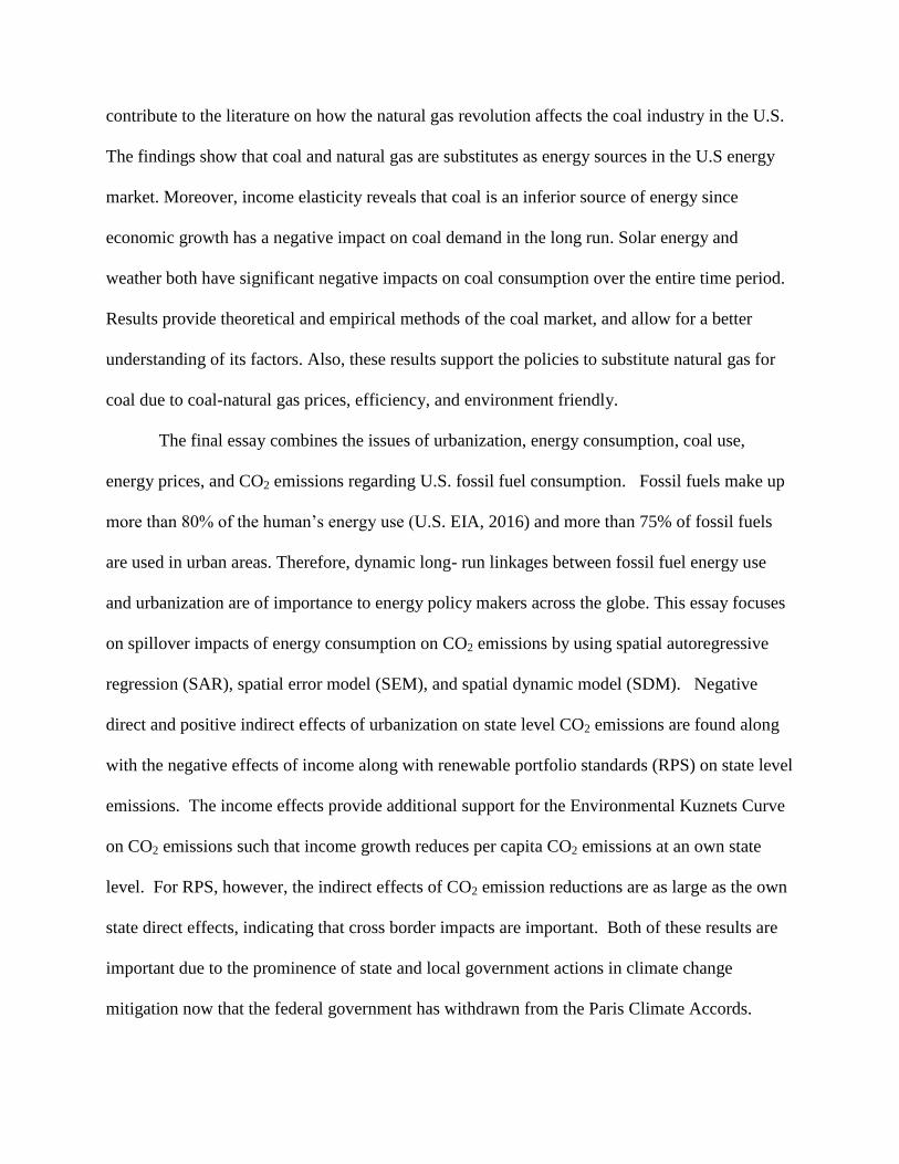