threat of grade retention, remedial education and student ...ftp.iza.org/dp7086.pdf · threat of...
TRANSCRIPT
DI
SC
US
SI
ON
P
AP
ER
S
ER
IE
S
Forschungsinstitut zur Zukunft der ArbeitInstitute for the Study of Labor
Threat of Grade Retention, Remedial Education and Student Achievement: Evidence from Upper Secondary Schools in Italy
IZA DP No. 7086
December 2012
Erich BattistinAntonio Schizzerotto

Threat of Grade Retention, Remedial Education
and Student Achievement: Evidence from Upper Secondary Schools in Italy
Erich Battistin University of Padova,
IRVAPP and IZA
Antonio Schizzerotto University of Trento
and IRVAPP
Discussion Paper No. 7086 December 2012
IZA
P.O. Box 7240 53072 Bonn
Germany
Phone: +49-228-3894-0 Fax: +49-228-3894-180
E-mail: [email protected]
Any opinions expressed here are those of the author(s) and not those of IZA. Research published in this series may include views on policy, but the institute itself takes no institutional policy positions. The IZA research network is committed to the IZA Guiding Principles of Research Integrity. The Institute for the Study of Labor (IZA) in Bonn is a local and virtual international research center and a place of communication between science, politics and business. IZA is an independent nonprofit organization supported by Deutsche Post Foundation. The center is associated with the University of Bonn and offers a stimulating research environment through its international network, workshops and conferences, data service, project support, research visits and doctoral program. IZA engages in (i) original and internationally competitive research in all fields of labor economics, (ii) development of policy concepts, and (iii) dissemination of research results and concepts to the interested public. IZA Discussion Papers often represent preliminary work and are circulated to encourage discussion. Citation of such a paper should account for its provisional character. A revised version may be available directly from the author.

IZA Discussion Paper No. 7086 December 2012
ABSTRACT
Threat of Grade Retention, Remedial Education and Student Achievement: Evidence from Upper Secondary Schools in Italy* We use a reform that was recently implemented in Italy to investigate the effects on academic achievement of more stringent requirements for the admission to the next grade at upper secondary school. We study how such effects are mediated by changes in family and school inputs, and in the student commitment to learn all school subjects including those usually considered as marginal components of the curriculum. Geographical discontinuities in the implementation of the reform allow us to set out the comparison of similar students undergoing alternative progression rules, and to shed light on whether, and to what extent, the reform has worked as a tool to improve short-term achievement gains. We document differential effects across curricular tracks, picturing at best – depending on the data employed – a marginal improvement for students in academic schools. We instead find sharp negative effects of the reform in technical and vocational schools, where the students enrolled come from less privileged backgrounds. These findings are accompanied by a substantial increase in the number of activities out of the normal school hours in technical and vocational schools, but not in academic schools. Also, we find that the reform has left unchanged the various family inputs that we consider, and that parents did not provide extra economic support to students facing an increased threat of grade retention. However, in contrast with the documented effects on achievement, we find that schools reacted to the additional administrative burdens and costs imposed by the reform by admitting more students to the next grade. We thus conclude that the reform has had a negative effect on motivation and engagement of the most struggling students, thus exacerbating existing inequalities. JEL Classification: C31, I24, I28 Keywords: policy evaluation, quasi experimental designs, remedial education Corresponding author: Erich Battistin University of Padova Department of Statistics Via Cesare Battisti 243-5 35123 Padova Italy E-mail: [email protected]
* This paper benefited from helpful discussion with Hans-Peter Blossfeld, Alfonso Caramazza, Piero Cipollone, Ilaria Covizzi, Roberto Cubelli, Daniele Checchi and from comments by audiences at Bamberg, Brescia, Verona, CORE, Stockholm and AERA 2012. Financial support from Fondazione Bruno Kessler is gratefully acknowledged.

1
1. Introduction
Increasing concerns about the quality of education in Europe and the United States
have lead in the recent years to the implementation of accountability policies designed to
hold administrators, teachers and students responsible for the level of academic
achievement. This strategy reflects the belief that the promise of rewards or the threat of
sanctions is needed to ensure change, setting clear standards and tools to promote
educational change (Hamilton, 2003). This paper assesses the effectiveness of a remedial
education reform that was recently introduced in Italian upper secondary schools with the
aim of improving student achievement. The intervention considered shares with
accountability policies the central assumption that sanctions may be an effective tool to
enhance performance.
Starting from the school year 2007/08, students in upper secondary schools of the
country who don’t meet predefined performance levels must attend remedial summer
courses, and their progression to next grade is conditional on passing a remedial exam
before the beginning of the new year. Remedial education assumes a more important role
in the formative plan, and is made compulsory during the school year for low performing
students. This new progression rule replaced the old system, in which students who were
not retained could be admitted to the next grade with ‘educational debts’ in one or more
subjects to be cleared with no clear deadline. According to this rule, the practice of social
promotion was effectively at work.
The policy question addressed in this paper is whether mandating remedial summer
courses for those deemed in need of such courses, and testing students after the summer
before admitting them to the next grade, makes a difference. In particular, we study the
short-term effects on student achievement, and how such effects are mediated by changes
in school and family inputs that are indirectly caused by the intervention. Our empirical
strategy exploits the quasi experimental variation that results from geographical
discontinuity in the implementation of the reform. Unlike the rest of the country, schools
located in a well-defined area of Northern Italy, the province of Trento, were exempted
from adopting the new progression system. We make use of this setting, and obtain
counterfactual quantities that we employ to quantify the effects of the reform.
Remedial exams were introduced in Italian schools in 1923, and were abolished in
upper secondary schools during the 1990s. The policy rationale for their reintroduction in
2007 resulted from a combination of scientific and political discussion on the evidence
2
from the first three waves of PISA of low performance of Italian students. Variability in
test scores across regions pictured a sharp North/South divide, with students in Northern
areas, amongst which the province of Trento, performing well above the OECD average.1
The policy implemented was therefore intended largely to provide strong incentives to
students, teachers and parents, thus reinforcing discipline and, though this, academic
achievement.
Advocates of the reform believed that the threat of grade retention was the most
effective device to control for low school performance. According to this interpretation,
students should study more intensely and, indirectly, achieve higher levels of proficiency
because individuals instinctively fair failure. From a theoretical point of view, this
assumption echoes the reinforcement theory originally developed by the behaviourist
school of psychology (see, for example, Staddon, 2003). However, the stimulus-response
mechanism alone may not be sufficient to account for all outcomes observed in learning
situations.2 By adopting this point of view, reform opponents raised the concern that the
threat of grade retention might undermine effort, motivation and engagement of struggling
students, thus exacerbating existing inequalities.
As a matter of fact, the desirability of grade retention policies as a method for
remediating poor performance is not uncontroversial. The recent push for educational
accountability has brought this policy problem back to the forefront. Despite the large
number of studies that have looked into this issue, evidence from quasi-experimental
designs is relatively scarce (notable exceptions are Jacob and Lefgren, 2004 and 2009). If
one considers only studies rigorously designed to control for selection bias, the available
evidence fails to demonstrate that grade retention is more beneficial than grade promotion,
for both academic and socio-emotional outcomes (see Jimerson, 2001, for a
comprehensive review of empirical findings). This paper marks something of a departure
from this literature, as we do not seek identification of the causal effects of retention on
1 As we shall see, it was mostly this evidence that motivated the discontinuity in the geographic roll out of the reform, although Trento was the only autonomous province in Northern Italy not complying with the new system. 2 The empirical evidence available suggests that intrinsic motivation (Fortier et al., 1996; Pintrich, 2003), social origins (Shavit and Blossfeld, 1993; Breen and Goldthorpe 1997; Bowles and Gintis 2002), parents’ behaviour and expectations (Englund et al., 2004), teachers’ expectations (Rosenthal and Jacobson, 1968; Saracho, 1991; Rubie-Davies et al., 2006), and teachers’ classroom assessment practices (McMillan, 2001) are inputs playing a pivotal role in the learning process, yielding heterogeneous reactions to punishment practices.

3
student outcomes. The quasi experimental comparison of outcomes for students
undergoing different progression rules is revealing of the threat.3
Overlaid to the dimension represented by retention policies, another relevant stream
of the literature that we touch upon is that investigating the effectiveness of remedial
education. The reform introduced clear requirements on the school side about the
organization of remedial courses for low achieving students, both during the school year
and in the summer for those mandated to the remedial exam. In investigating the reduced
form effects of the reform, we compare outcomes in areas implementing different
progression rules without distinguishing the relative merits of remedial instruction time
vis-à-vis the increased threat of grade retention. Disentangling the causal effects of these
two channels calls for empirical evidence on remedial education for underperforming
students. However, rigorous research in this direction is still scanty, and points to mixed
results. Lavy and Schlosser (2005) quantify the effects of a remedial intervention for high
school students in Israel, finding a significant increase in the school mean matriculation
rate. Calcagno and Long (2008) look at the impact of post-secondary remediation
programmes in Florida, finding that mathematics and reading courses have mixed benefits
on college performance. Battistin and Meroni (2012) investigate the short term effects for
low achieving students in Italian lower secondary schools, and document positive results
for mathematics but not for reading.
Our analysis adds to the empirical findings documented in economics, sociology and
psychology on the interplay between incentives faced by students and academic
achievement. Effort, total time devoted to study and engagement at school were found to
be important determinants of student learning (see, for example, the review by Bishop,
2004). Students choose which subject to focus on, and decide how much effort to put into
each task. Depending on the incentives facing students, one may expect sizeable
differences in decisions about effort. The available empirical evidence suggests that
determinants of effort may vary a great deal across school tracks. For example, Carbonaro
(2005) finds that students in higher curricular tracks exert substantially more effort than do
students in lower tracks. This, of course, may simply reflect differences in effort explained
by sorting of students into tracks. However, given the very rich set of background and
3 To the best of our knowledge, the closest in spirit to our paper is the work by Belot and Vandenberghe (2011), who study the effects of the threat of grade retention introduced by a reform implemented for the French speaking community in Belgium finding no effects on achievement gains.

4
school characteristics controlled for in the analysis, Carbonaro (2005) claims that the
differences documented are suggestive of track specific effects on effort. This evidence is
reinforced if one considers the work by Hastings et al. (2012), who provide quasi-
experimental evidence that school choice has sizeable effects on motivation and academic
performance for low income and minority students. It is well documented that setting
higher standards in schools may induce heterogeneous effects on effort, having adverse
consequences on students for whom standards move beyond their reach. For example,
Betts and Grogger (2003) find that high standards have significantly larger returns on test
scores at the top end of the ability distribution. This result may be mediated by differential
effects on effort, as students at the bottom end of the distribution may perceive themselves
as losing ground and give up.4
Gender differences in decisions about effort are a relevant dimension to consider. The
attitude of female students is more supportive of academic learning than that of their male
peers (see, for example, Carbonaro, 2005). This implies that there might be positive
externalities in classes or schools with higher percentage of females. Lavy and Schlosser
(2011) study the effects of classroom gender composition on academic achievement,
finding that both male and female students tend to perform better in classes presenting
higher percentages of females. They find heterogeneous effects depending on the
socioeconomic background of students, with larger effects for the most disadvantaged
groups. In documenting the channels for the existence of such gender peer effects, Lavy
and Schlosser (2011) find that having more female students in the class has positive
effects on the learning climate and inter-student relationships, thus leading to a more
efficient use of instructional time. This should affect positively non-cognitive factors like
motivation and concentration and thus, indirectly, learning.
The above findings suggest that a sensible stratification to consider for the empirical
analysis is by gender and curricular track. This is what we will do in documenting the
main results. Technical and vocational schools in Italy are characterised by a much lower
proportion of female students in the class when compared to academic schools. It is well
documented in the literature that not only students perform better if their peers are high
achievers, but peers can also act as a buffer by legitimising deviant behaviour. Thus, it is
4 For example, Betts and Grogger (2003) document differential effects of setting high standards by ethnicity, with lower returns on achievement for blacks. This is consistent with findings by Carbonaro (2005), who documents, ceteris paribus, lower effort from black students.
5
interesting to investigate how the increased threat of sanctions induced by the reform
interacts with gender, and with differences in the learning climate. The stratification by
gender is also motivated by studies that have documented gender differential in skills that
may depend on the mode of assessment.5
Our empirical analysis is conducted using survey and administrative data from
complementary sources of information that we were able to obtain for the purpose of this
study. Test scores and socio-economic indicators come from a small scale survey that was
commissioned purposively for the evaluation of the reform in selected schools either side
of the administrative border of the province of Trento. This information is complemented
with data from the PISA 2006 and 2009 surveys, as they refer to pre and post-policy
periods. We were able to obtain from the Ministry of Education area identifiers for where
the schools are located, not available in the public use files, so to reproduce fairly closely
the same evaluation design considered for the main analysis. Finally, we use time series
data coming from administrative information released by the Ministry of Education on
retention rates for all schools in the areas considered for the evaluation.
The main findings of this paper can be summarized as follows. First, we find sharp
differences depending on the type of school considered, and thus on the socio economic
background of students. Consistently across data sources, we document negative effects of
the reform on academic achievement in vocational schools. As for academic schools, in
the main analysis we find no statistically significant effect, which becomes positive and
significant in some dimensions of learning once we employ PISA data as a sensitivity
check. Because of the importance of distributional effects, we go beyond averages and
assess how the intervention considered affects achievement across quantiles of the test
score distributions. We find that much of the variability in the effect is captured through
the stratification by curricular track, and document much lower within track differences
across students. Most interestingly, we find more pronounced negative effects for females
in vocational tracks, where the proportion of male students is higher. The results are
5 For example, Machin and McNally (2005) find lower achievement of female students resulting from the introduction of the National Curriculum in the United Kingdom, that set out the standards that should be achieved at different stages of the education sequence and, amongst other things, assigned more importance to continuous assessment by teachers. Gipps and Murphy (1994) report evidence that females do less well in timed examinations because of higher levels of anxiety. Powney (1996) reviews a number of studies documenting that the mode of assessment is a factor explaining the differential performance of male and female students. Pekkarinen (2012) provides evidence that the structure of the educational system affects male and female students differently, in particular with reference to tracking in secondary schools.

6
robust to sensitivity checks that we perform on the functional form adopted, as well as the
source of identifying variability employed. Thus, consistently with the findings in Betts
and Grogger (2003), our first contribution is to show that higher standards coming with
the threat of sanctions contribute considerably to create inequality in the distribution of
educational achievement, resulting in both winners and losers.
Second, we use PISA data to investigate the effects of the intervention on key inputs
of the education production function, providing important insights on the possible
mediating factors driving the results documented above. We find no significant effects of
the reform on household spending for education, the bulk of which - given the public
school system in Italy - consists in fees paid to individual teachers in the school or to other
teachers for tutoring. According to our findings, households ceteris paribus did not react
to the reform by providing extra support to students facing an increase in the threat of
grade retention. In contrast, we find that the amount of extra time spent by students
learning subjects outside of normal school hours increased after the reform. Of course this
effect could be explained as a mechanical consequence of the intervention itself, being the
provision of remedial classes for low achieving students compulsory on the school side.
However, our results show that much of the action took place in technical and vocational
schools, while in academic schools the provision of remedial classes is unaffected by the
reform. From this evidence we conclude that the reform lowered the “safety” of the most
struggling students, imposing substantial extra work loads only for those from low socio-
economic backgrounds.
Third, we document the effects on the promotion and retention rates for the two
groups of schools considered during the first three school years following the reform. We
compare the status of students in June of each year in areas affected by the reform (i.e.
“admitted to the next grade”, “retained” or “mandated to summer courses and the remedial
exam in September”) to the status of students in areas that we use as controls (i.e.
“admitted to the next grade”, “retained” or “admitted to the next grade with ‘educational
debts’”). Despite the effects on achievement documented above, we find that the reform
sensibly increased the percentage of students in vocational schools admitted to the next
grade in June of each year. The same conclusion holds for academic schools, although the
results documented are only marginally significant. On the contrary, we find - consistently
across curricular tracks - no effect on retention rates in June, thus concluding that schools
reacted to the reform by admitting to the next grade students who, before, would have
been given an ‘educational debt’. Since the mandatory organisation of remedial summer
7
classes for low achieving students impacts importantly on school budgets, we interpret this
result as adaptive behaviour that resulted in less stringent rules to pass students to the next
grade. Thus we conclude that the effects documented on achievement are driven by
important changes in school inputs. Our findings highlight the importance of providing
schools with sufficient resources to support general reforms of the school system that are
aimed at enhancing the competences of students. The relevance of this problem for policy
making is particularly important for students and areas facing marked socio-economic
deprivation, and thus being at risk of lagging behind in their development.
Finally, we perform back of the envelope calculations to infer the long term effects of
the reform on graduation rates at upper secondary school. To this end, we exploit a
different education reform that took place in the country during the 1990s and, curiously
enough, represents the mirror image of the intervention considered in this paper. The
reform was rolled out starting from the school year 1994/95, and introduced the practice of
the ‘educational debt’ by abolishing the same remedial exam in September that was again
introduced in 2007/08. We use data from the Bank of Italy Household Survey on Income
and Wealth to set out the comparison of cohorts of individuals aged 14 during the 1990s,
14 being the normal age for completing compulsory schooling at the time. Bearing in
mind some important differences between the two reforms that we discuss in what
follows, the cohort study that we set out points to no effects of the threat of grade retention
on attainment of the upper secondary school diploma.6
The remainder of the paper is organised as follows. The main features of the policy
under evaluation are discussed in Section 2. Section 3 presents the data, while the
evaluation design is illustrated in Section 4. Results are reported in Section 5. Conclusions
and policy implication are discussed in Section 6.
6 A similar result is found by Belot and Vandenberghe (2011). Differently from the most recent counter-reformation, remedial courses for low achieving students were not mandatorily included in the school formative plan during the 1990s. It thus follows that the cohort study that we set out reveals the long-term effects of ‘educational debts’ vis-à-vis the increased risk of grade retention represented by the remedial exam in September. We could in principle consider other variables that refer to labour market outcomes later in life, as well as university participation and attainment. We however show that the cohorts of students affected by the 1994/95 reform were also affected by an additional reform of the university system in the early 2000s, thus making it difficult to disentangle the effects of the various interventions on outcomes such as university degree and wages.

8
2. Background
Until the school year 2006/07, students in upper secondary schools in Italy who were
not retained could be admitted to the next grade with or without an ‘educational debt’
(debito formativo), that is a final mark signaling the lack of predefined performance level
in one or more subjects. Such lack in achievement was given at the end of the school year
(mid-June), and was to be cleared in the following years with no clear deadline. The
system at work de facto resulted in the practice of social promotion. Official figures
provided by the Italian Ministry of Education show that about 42 percent of students
enrolled at high school in the country were given at least one educational debt, with just
one out of four students recovering it by the end of the following year.
Table 1 presents descriptive statistics for the school year 2006/07 derived by the
Ministry of Education, using all upper secondary schools in the areas considered for the
main analysis. Separately for academic and technical/vocational schools, reported are the
percentage of students retained, the percentage of students with at least one educational
debt and the end of the school year, and a breakdown of debts assigned by subject. Results
are presented by gender, as this dimension will prove particularly important in our
empirical analysis. Numbers reported refer to the first two upper secondary school grades,
as these define the relevant age band for students in our sample.
Retention rates in vocational schools are much higher than in academic schools, for
both males and females. Gender differences are clearcut, with females performing sensibly
better than males across schools and grades. The difference across schools almost vanishes
when it comes to educational debts, gender remaining the most relevant dimension. Above
40 percent of males are given at least one educational debt, and this figure is roughly the
same across school types. The percentage for females with educational debts is well below
that for males, and females in vocational schools are marginally worse than their peers in
academic schools. The breakdown by subject reveals that mathematics and foreign
languages are, by far, the most problematic subjects, with no clear pattern by gender.
These numbers, which provide a representative picture of the situation in Italy in the
early 2000s, casted doubts on the learning effectiveness of the upper secondary system,
and the need for a general reform of the school curricula was brought to attention. The

9
disappointing output documented by the first three PISA surveys created even more
concern in the public opinion.7
A major intervention was therefore implemented starting from the school year
2007/08 to enforce the recovery of educational debts. There are three key factors that
characterized this reform (which the media called the “Fioroni reform” from the name of
the Minister of Education in place). First, under the new progression system, which is still
in operation, students in upper secondary schools were compelled to recover all
educational debts before the beginning of the new year (mid-September). Second, students
with educational debts must attend remedial courses organized by the school during the
summer, and take a remedial exam in early September (the assessment mode being
decided by the school). On failing to pass the exam, retention would be deliberated by the
school council. Finally, the reform introduced more stringent requirements on the school
side about the organization of summer courses. Although we were not able to access
administrative data on school budgets for a large enough number of cases, it is well known
to researchers and policy makers that the additional burdens imposed by the reform were
not compensated by an adjustment of financial resources transferred from the Ministry of
Education to the schools. It is thus fair to conclude that schools complied with the
requirements of the new progression system administrating the same financial resources
employed in the past.
Contrary to what happened in the rest of the country, the local government of the
province of Trento, an area of Northern Italy which enjoys some degree of autonomy in
the implementation of education policies, did not comply with the reform. The decision
was made moving from the available evidence on the achievement of students enrolled in
local schools. Italy is characterized by substantial variability in PISA scores across areas,
with students in Northern regions performing well above the national average. At the time
of the reform, PISA scores for students living in the province of Trento were as good as
those recorded by top-ranking countries.8 In light of this evidence, local policy-makers
7 According to PISA 2000 data, Italy ranked above Spain, Portugal and Greece but far behind the most advanced countries. The average score of Italian students was 100 points lower than that of top-ranking Korean students (OECD 2001). The public concern became widespread after the PISA 2003 results for mathematics, when the overall performance of Italian students dropped below that of Spain and Portugal with an average score of 86 points lower than that of their Finnish peers (OECD 2004). The overall picture was confirmed in the PISA 2006 survey (OECD 2007). 8 For example, according to PISA 2006 data the average test score in mathematics is 462 in Italy, and 508 in the province of Trento. The same sharp difference remains if test scores in reading comprehension and scientific literacy are considered.
10
decided that there was no need to comply with the national intervention. Furthermore, they
supported the idea that remedial courses already offered to students by schools in the
province were effective for the full recovery of educational debts, and that no remedial
exam was needed to ensure the achievement of academic standards.
We exploit such geographic discontinuity to investigate the short-term effects of the
reform on a variety of outcomes. The question is whether mandating remedial summer
courses for low performing teenagers, and tight their promotion to the exam in September,
makes a difference. In addition to the direct effect on achievement, which may be
mediated by the effect on effort, there may be an indirect effect of the reform on the
attitude of parents towards the education of their children. For example, reacting to the
threat of grade retention, parents may decide to increase household spending for fees paid
to teachers for tutoring. Similarly, there may be effects on the school side, as the
organization of summer courses imposed by the reform may come at some cost, and this
may vary depending on the resources available at the school. The aim of the next section
is to describe the data that we employ to shed light on these aspects.
3. Data
3.1. Main sample
The data set combines school administrative databases (containing teachers’ marks
and information on promotion/retention) and unique data from two surveys purposively
designed for this study. The first survey collects information on student proficiency
through the administration of a standardized assessment test to all students in our sample.
The second survey – administered to parents – collects information on parental social
background such as education, job status, household composition and learning resources at
home.
The assessment methodology was shaped around PISA, and adjusted to the specific
purpose of our study. The test was developed from publicly released items from the first
three PISA assessments available at the time that this research started (2000, 2003 and
2006). The test was constructed by experts at the Ministry of Education to guarantee
comparability of items difficulty with the PISA scale, and was conducted at the beginning
of the 2008/09 school year (October/November 2008).9 Students were asked to provide
9 The items were presented to students in three one-hour booklets, resulting in a three-hour session with 23 units for reading, 20 for mathematics and 19 for science. All students in our sample took the same tests, thus

11
information about education and occupation of their parents, and life-style at home. An
additional survey was carried out on parents soon after the test. Respondents were asked to
provide detailed information on educational and employment background, household
composition and home learning resources.
The sampling frame for the survey was constructed by considering a selected number
of towns sharing similar characteristics in terms of their demographic, economic and
occupational structure, as well as of school-related infrastructures (see Figure A.3 of the
Appendix). To ensure comparability, we considered towns near the administrative border
of the province of Trento. The leading criteria followed to guide selection were (i) the
presence of schools for each curricular track of the Italian upper secondary school system:
licei (academic, or general education, track), istituti tecnici (technical track) and istituti
professionali (vocational track); (ii) population size of town; and (iii) features of the
economic and occupational structure. A pair-wise matching comparison of towns was
conducted, which was further refined by controlling for geographical proximity (less than
seventy kilometers). As a result of this procedure, we ended up selecting three towns in
the province of Trento and their most similar counterparts outside the administrative
border. The population of the three town considered covers approximately one third of the
total population of the province of Trento.
The target sample of students resulted from a two-stage procedure that selected
schools in the first stage, and in the second stage cohorts of students defined from the year
attended at the time of the test. We again followed a one-to-one matching procedure,
selecting similar schools located in each pair of towns. The selection of schools was
conducted by controlling for observable dimensions such as school track, school size as
measured by trends in enrollment and school resources, as well as unobservable
dimensions (such as reputation of the school) gathered from general knowledge of the
socio-economic background in which they operate.
Across all schools, we focused on students attending the second and the third upper
secondary grade during the school year 2008/09, thus aged between 15 and 16. For each
school we randomly selected two classes in the second year (i.e. for the cohort of students
enrolled for the first time in school year 2007/08) and two classes in the third year (i.e. for
leaving us with the joint distribution of test scores for the three dimensions of learning considered (reading, mathematics and science). Following the OECD procedure test scores were obtained from item response theory, and standardised using mean and standard deviation of PISA 2006 scores in the province of Trento.

12
the cohort of students enrolled for the first time in school year 2006/07). We did so to
ensure variability in the duration of enrollment at school across the different regimes
defined by the reform. The cohort dimension proved statistically not important in the
analysis, and will not be considered in what follows.
Information on student achievement was complemented with administrative data
on teachers’ marks on past years at school, as well as with the final grade students
obtained at the state examination on completion of the lower secondary school (leaving
certificate). Qualitative data elaborated from interviews conducted with all school
principals completed the sources of information that will be used for our empirical
exercise. The sample size of the working data, which in what follows we will refer to as
“Main Sample”, is reported in Table 2. The number of schools involved in the analysis is
22. The number of students is 916 and 942 inside and outside the province of Trento,
respectively, evenly distributed in academic and vocational tracks.10
3.2. Additional sources of information
Test scores for the main sample were collected in October/November 2008. It
follows that the identification strategy employed to measure the effects on achievement
may only use post reform data. We complemented this information with data for pre
reform periods coming from the PISA 2006 and 2009 surveys, and used information from
these two waves to assess the sensitivity of our conclusions obtained from the main
sample to the presence of selection bias.
The Ministry of Education granted us access to information which is not available
in public use PISA files, allowing us to select (academic and vocational) schools in
narrowly defined areas that match closely the evaluation design described in the previous
section.11 The resulting sample, which in what follows we will refer to as “PISA Sample”,
contains test scores for students before (PISA 2006) and after (PISA 2009) the reform roll
out. Given that the nature of the information collected, the set of demographics in the main
10We investigated the possible sorting effects deriving from the choice of curricular track at high school across the areas considered in our analysis. We computed the average transition rates from lower secondary school to licei for the school year 2007/08 using official data from the Ministry of Education. This analysis pictures rather similar figures in the areas considered, with transition rates ranging between 29 and 34 percent. 11 Because of the design of the PISA survey, in which repeated cross sections of schools are sampled at each wave, we were not able to identify the same schools as in the main sample. Moreover, the finest area identifier that we were able to gather is the province where schools in the main sample are located - an Italian province being a territory administratively similar to a US county.

13
sample coincide with those available in the PISA sample. Sample size for the latter dataset
is reported in Table 2.
Finally, we were able to gather administrative data from local government agencies
and the Ministry of Education on retention rates since the school year 2006/07 in the areas
considered for the evaluation. We constructed longitudinal information for the same
schools included in the main sample, thus picturing changes in retention rates from before
to after the reform that come on top of school-specific fixed effects. We will use this
information to document how schools reacted to the reform, and to relate this to the
documented effects on achievement.
4. Methods
4.1 Identification strategy
The evaluation design sets up the comparison of outcomes for students in upper
secondary schools in the province of Trento, to outcomes for students in similar schools in
adjacent areas. The causal interpretation crucially rests upon a ceteris paribus condition
about the composition of students and inputs in the two groups of schools. This amounts
to assuming that the outcome for students enrolled in one group of schools can serve as an
approximation to the counterfactual outcome for students enrolled in the other group of
schools.
The general problem underlying the validity of this condition can be easily put across
using standard arguments taken from the programme evaluation literature (see, for
example, Heckman and Vytlacil, 2007). In the potential outcomes framework interest lies
in the causal impact of a given “treatment” on an “outcome” of interest. Let 𝑌1 (𝑌0) denote
the potential outcome that would result from the remedial exam being (not being) in
operation. The causal effect of the reform on school achievement is then defined as
𝑌1 − 𝑌0. This difference is by its very nature not observable, as geographical location of
the school attended reveals only one of the two potential outcomes (𝑌0 for students in the
province of Trento, and 𝑌1 otherwise).
The average policy impact for students facing remedial exams (or the average
treatment effect of the reform on the treated) is defined as:12
12 The notation 𝐸𝐴|𝐵[𝐴|𝑏] and 𝐹𝐴|𝐵[𝑎|𝑏] indicates the conditional expectation and distribution, respectively, of the random variable 𝐴 given 𝐵 = 𝑏.
14
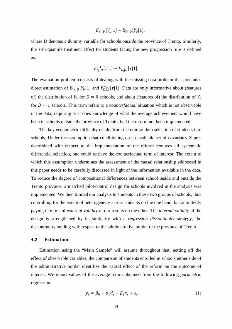
𝐸𝑌1|𝐷[𝑌1|1]− 𝐸𝑌0|𝐷[𝑌0|1],
where D denotes a dummy variable for schools outside the province of Trento. Similarly,
the 𝜏-th quantile treatment effect for students facing the new progression rule is defined
as:
𝐹𝑌1|𝐷−1 [𝜏|1] − 𝐹𝑌0|𝐷
−1 [𝜏|1].
The evaluation problem consists of dealing with the missing data problem that precludes
direct estimation of 𝐸𝑌0|𝐷[𝑌0|1] and 𝐹𝑌0|𝐷−1 [𝜏|1]. Data are only informative about (features
of) the distribution of 𝑌0 for 𝐷 = 0 schools, and about (features of) the distribution of 𝑌1
for 𝐷 = 1 schools. This term refers to a counterfactual situation which is not observable
in the data, requiring as it does knowledge of what the average achievement would have
been in schools outside the province of Trento, had the reform not been implemented.
The key econometric difficulty results from the non-random selection of students into
schools. Under the assumption that conditioning on an available set of covariates X pre-
determined with respect to the implementation of the reform removes all systematic
differential selection, one could retrieve the counterfactual term of interest. The extent to
which this assumption undermines the assessment of the causal relationship addressed in
this paper needs to be carefully discussed in light of the information available in the data.
To reduce the degree of compositional differences between school inside and outside the
Trento province, a matched pilot/control design for schools involved in the analysis was
implemented. We then limited our analysis to students in these two groups of schools, thus
controlling for the extent of heterogeneity across students on the one hand, but admittedly
paying in terms of external validity of our results on the other. The internal validity of the
design is strengthened by its similarity with a regression discontinuity strategy, the
discontinuity holding with respect to the administrative border of the province of Trento.
4.2 Estimation
Estimation using the “Main Sample” will assume throughout that, netting off the
effect of observable variables, the comparison of students enrolled in schools either side of
the administrative border identifies the causal effect of the reform on the outcome of
interest. We report values of the average return obtained from the following parametric
regression:
𝑦𝑖 = 𝛽0 + 𝛽1𝑑𝑖 + 𝛽2𝑥𝑖 + 𝜀𝑖, (1)
15
which is estimated separately for the various groups considered (gender and curricular
track). Results from this specification will be reported in Table 5.
We considered semi-parametric alternatives to this specification, which we used to
check the sensitivity of our conclusions to the estimation method employed. First, the
average effect of interest was estimated through a matching estimator, contrasting
outcomes across pairs of similar students in schools undergoing different progression
rules. Matching was implemented using the propensity score, which was obtained from a
parametric regression of the “treatment” status on the observables that will be described in
the next section. Estimates of the propensity score are reported in columns (5) and (10) of
Table 3. Second, we employed the same propensity score to estimate the average effect
through a weighting estimator (see, for example, Imbens, 2004). Perhaps not surprisingly
given the evaluation design adopted, the two groups of students contrasted were
characterized by substantially identical distributions of the rich set of observables
controlled for, thus ruling out any type of common support problem in the data. We
however check the robustness of our results dropping from the sample observations that
were extreme with respect to the propensity score metric. The various sensitivity checks
considered yielded results equivalent to those obtained from the estimation of the
parametric regression in (1), both in terms of point estimates and statistical significance.
Because of this, we decided to report only parametric estimates while presenting the
results in the following sections. Estimation results obtained using the weighting
procedure described in Imbens (2004) are presented in Table A.1 of the Appendix.
In estimating quantile treatment effects from the “Main Sample”, we decided to fit the
standard quantile regression counterpart of equation (1). The results from this analysis will
be presented in Figure 1. We checked the sensitivity of our findings to alternative
estimation methods employed in the programme evaluation literature (see, for example,
Firpo, 2010), but the results proved very similar to those presented in the main text (see
Figure A.1 of the Appendix).
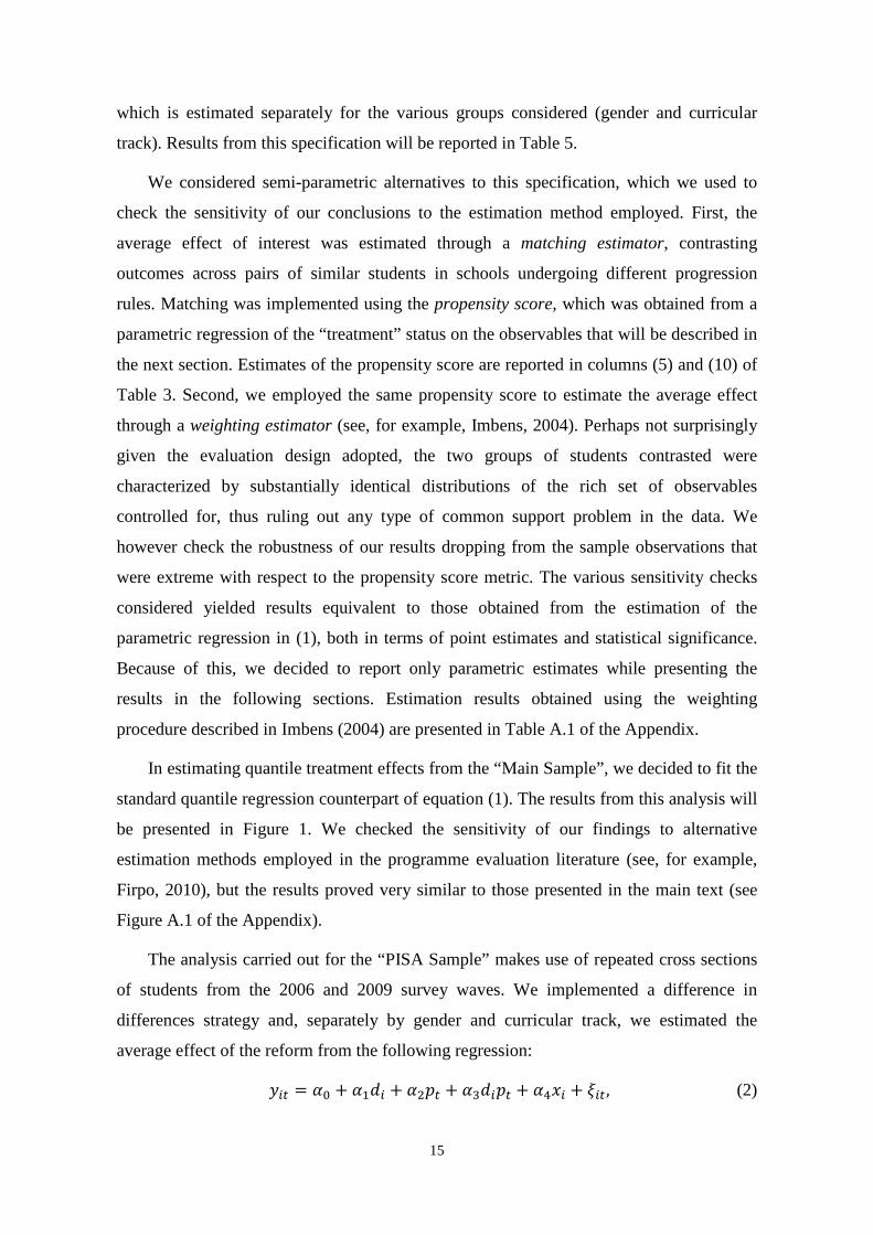
The analysis carried out for the “PISA Sample” makes use of repeated cross sections
of students from the 2006 and 2009 survey waves. We implemented a difference in
differences strategy and, separately by gender and curricular track, we estimated the
average effect of the reform from the following regression:
𝑦𝑖𝑡 = 𝛼0 + 𝛼1𝑑𝑖 + 𝛼2𝑝𝑡 + 𝛼3𝑑𝑖𝑝𝑡 + 𝛼4𝑥𝑖 + 𝜉𝑖𝑡, (2)

16
where 𝑝𝑡 is a dummy for observations coming from the post reform survey round. The
socio-economic demographics controlled for in the analysis coincide with those
considered in equation (1). As before, semi-parametric alternatives to (2) were considered
as a sensitivity check (Abadie, 2005), which yielded informationally equivalent results and
are not reported in the main text. The average effect of the policy, 𝛼3, and the extent of
pre-policy differences across areas, 𝛼1, are the parameters of interest in (2). The former
parameter is compared to 𝛽1 estimated from equation (1). The latter parameter serves as a
over-identification test for the validity of the conclusions drawn from the “Main Sample”:
should the evaluation design be properly conducted, no difference in test scores across
areas in 2006 must be detected, after having netted off the effect of the observables X. The
results from this analysis are presented in Table 6 and Table 7.
Finally, administrative data for schools were used to run the following regression:
𝑦𝑖𝑗𝑡 = 𝛾0 + 𝛾1𝑝𝑡 + 𝛾2𝑑𝑖𝑝𝑡 + 𝛾𝑗 + 𝛿𝑖 + 𝜈𝑖𝑡, (3)
which models the outcome change (e.g. retention rates) at grade j for school i from before
to after the implementation of the reform, controlling for both school (𝛿𝑖) and grade (𝛾𝑗)
fixed effects. We will consider the results from the specification to look into the effects of
the reform on school inputs, using micro data at the school level from the Ministry of
Education. The results will be reported in Table 8.
Throughout the analysis, we will compute standard errors which are robust to
heteroskedasticity and are clustered at the class level. When using PISA and
administrative data, the cluster unit that we consider is the school.
5. Results
5.1 Descriptive statistics
Table 3 provides a picture of the degree of homogeneity for students in the two
groups of schools along the key dimensions relevant for the analysis. Data from the “Main
Sample” are considered for the following covariates: (i) student demographics (gender,
age, dummy for foreign students, dummy for cohabitation with mother and father,
proximity to school) (ii) socio-economic background of the household (father’s age and
education, mother’s age and education, dummy for housewife mothers, dummy for
unemployed mother or father), (iii) household wealth and social-status(occupational

17
stratification scores, material deprivation index).13 Means and standard deviations of these
variables are reported, stratifying observations by curricular track and policy status. To
test for the validity of our evaluation design, we estimated the propensity score from a
regression of the dummy for being a student in schools outside the province of Trento on
the covariates considered. Results from this regression are reported in columns (5) and
(10) of the table, for academic and vocational tracks, respectively. Overall, the distribution
of demographics is balanced across the two groups of areas, although some departure from
the general pattern emerges for the education level of mothers. Regardless of the index
considered, the difference in socio-economic backgrounds between students enrolled in
vocational vis-à-vis academic schools is worth noting.
The bottom panel of the table reports descriptive statistics for test scores in the
three dimensions of learning considered by PISA. Taken at face value, the mean
difference between the two groups of areas is positive for academic schools, and negative
for vocational schools. Table 4 adds in the additional dimension represented by gender
differences. The average test score for the three domains considered is considerably lower
for students enrolled in technical and vocational schools compared to students in academic
schools. Students in the former group of schools undergoing the new progression rule
present levels of reading, mathematical and scientific literacy lower than those of their
counterparts in the province of Trento. Simple tests for the significance of the outcome
difference between policy on and policy off areas point to positive results for males in
academic schools for the science test score, and negative results for females in technical
and vocational schools for the reading and science test scores. The results are therefore
suggestive of disparities in achievement between treated and control schools, with
negative differences for females from lower socio-economic backgrounds.
For descriptive purposes, we used the “PISA Sample” to investigate the
distribution of other key school inputs that may concur to determine test scores for
students in the two areas. In particular, we considered the student to teacher ratio and the
proportion of girls in the class, which produced roughly equivalent figures either side of
the administrative border of the province of Trento and stable across survey waves.
13 The socio-economic status is measured using an Italian occupational stratification scale that measures the social desiderability (and, in broad sense, the prestige) attributed to different jobs (De Lillo and Schizzerotto, 1985). The life style deprivation index (Whelan et al., 2002) is an additive index based on the lack of 5 items in the household: TV, car, DVD player, computer, internet access. Each individual item is weighted by the proportion of households possessing that item in Italy. Weights were derived from the SILC 2006 survey for Italy.
18
Academic schools present a teacher to pupil ratio equal to 8.65 and 8.01 inside and outside
the province of Trento, respectively. The corresponding figures for technical and
vocational schools are instead 6.49 and 7.27. As we have anticipated in the Introduction,
the average proportion of girls in the latter curricular track is way below that in academic
schools, being 44 percent in the province of Trento vis-à-vis 41 percent outside the
province. These should be compared with the values 66 percent and 67 percent,
respectively, for academic tracks. It is thus fair to conclude that the stratification by
curricular track that we maintain throughout the analysis captures sensibly different
environments for the class, both in terms of socio-economic background and climate
learning.
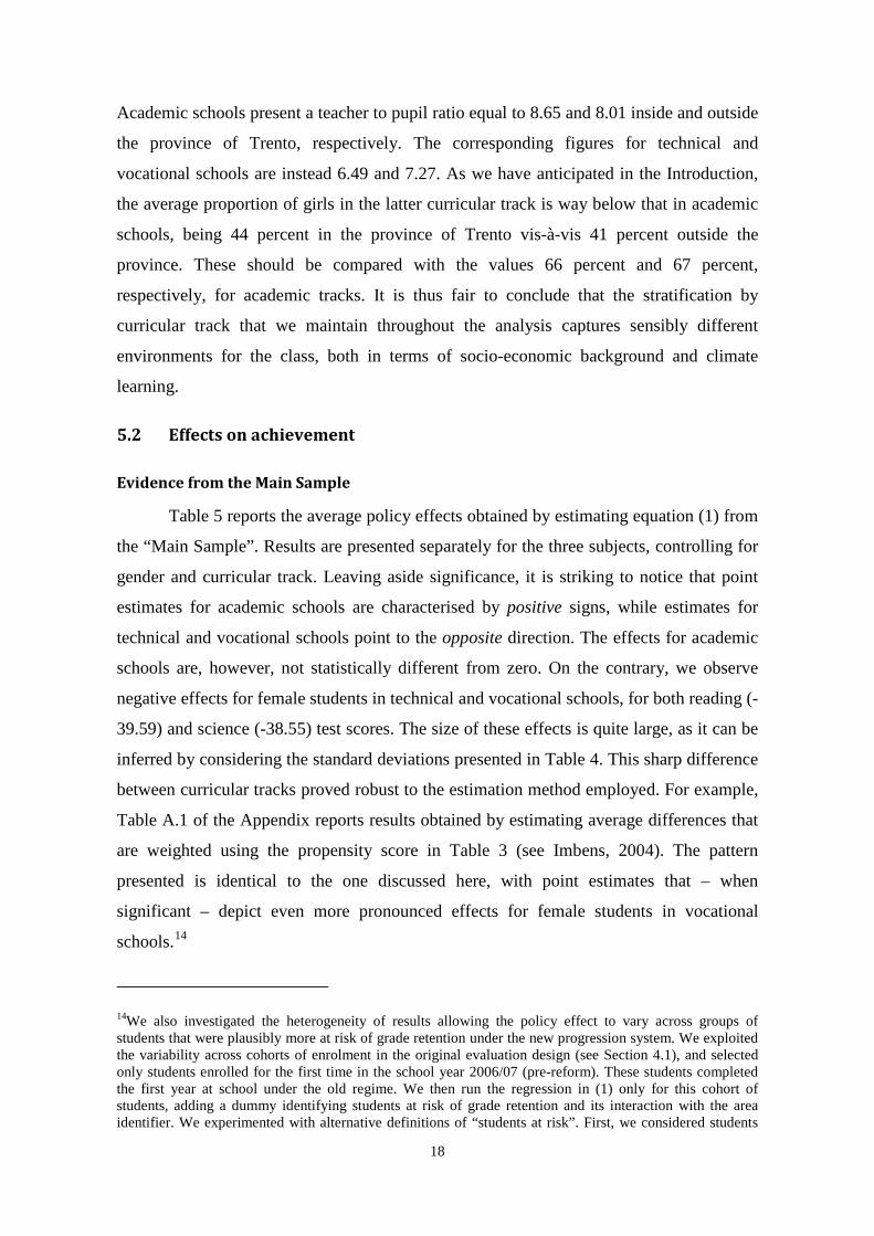
5.2 Effects on achievement
Evidence from the Main Sample
Table 5 reports the average policy effects obtained by estimating equation (1) from
the “Main Sample”. Results are presented separately for the three subjects, controlling for
gender and curricular track. Leaving aside significance, it is striking to notice that point
estimates for academic schools are characterised by positive signs, while estimates for
technical and vocational schools point to the opposite direction. The effects for academic
schools are, however, not statistically different from zero. On the contrary, we observe
negative effects for female students in technical and vocational schools, for both reading (-
39.59) and science (-38.55) test scores. The size of these effects is quite large, as it can be
inferred by considering the standard deviations presented in Table 4. This sharp difference
between curricular tracks proved robust to the estimation method employed. For example,
Table A.1 of the Appendix reports results obtained by estimating average differences that
are weighted using the propensity score in Table 3 (see Imbens, 2004). The pattern
presented is identical to the one discussed here, with point estimates that – when
significant – depict even more pronounced effects for female students in vocational
schools.14
14We also investigated the heterogeneity of results allowing the policy effect to vary across groups of students that were plausibly more at risk of grade retention under the new progression system. We exploited the variability across cohorts of enrolment in the original evaluation design (see Section 4.1), and selected only students enrolled for the first time in the school year 2006/07 (pre-reform). These students completed the first year at school under the old regime. We then run the regression in (1) only for this cohort of students, adding a dummy identifying students at risk of grade retention and its interaction with the area identifier. We experimented with alternative definitions of “students at risk”. First, we considered students

19
We checked the sensitivity of these findings to omitted variable bias by relying on
within student variability in achievement. This idea is not novel, and was already
employed in other studies (see, for example, Lavy et al., 2012). We considered the various
teacher marks available in the data as indicators of performance, pooled them with the
three tests scores collected through the main survey (reading, mathematics and science),
and derived a proxy for student “ability” according to the following procedure. First, for
each student we considered final marks at the end of the two semesters of the first and
second grade at school, for both mathematics and Italian language. We limited the analysis
to these subjects as they are common across all curricular tracks. We also considered the
final mark obtained at the end of the lower secondary school. This yielded a total of 8 to
12 indicators per students, depending of the cohort of enrollment in the original sampling
frame (see Section 3.1). Second, we stacked these indicators and run gender-specific fixed
effect regressions controlling for subject dummies (mathematics or science, vis-à-vis
reading or Italian language), nature of the indicator employed (test scores vis-à-vis
administrative marks) and age when the indicator was measured. Third, we used these
regressions to predict student level fixed effects, that we inserted into (1) to net off
unobservables that can be related to ability of students, or unobserved family background
characteristics.
Results from this specification are reported in Table A.2 of the Appendix, which
aligns well with the pattern already documented in Table 5. In technical and vocational
schools, only test scores for female students are affected by the reform. The negative
effects documented for reading and science are still confirmed, although their magnitude
is now somewhat attenuated. Differently from before, the effect for mathematics is now
statistically significant, and positive. As for academic schools, most of the results in Table
5 are confirmed. The negative effect of reading for males, which was not statistically
different from zero, is now more precisely estimated and significant at the conventional
levels.
Consistently with other studies in the literature, we went beyond averages and
tested whether the reform affected achievement across quantiles of the distribution of test
who were admitted to the second grade with at least one educational debt. Second, we focussed on students having a debt in mathematics, as we know from Table 1 that this was, by far, the case most frequently encountered situation. Finally, we defined at risk those students who completed the lower secondary school with the minimum score. As expected, results from this set of regressions show that students more at risk of grade retention have actually lower test scores that their peers in the class. However, we rejected the hypothesis that the results documented in Table 5 vary with risk.

20
scores. Figure 1 reports the values of the quantile treatment effects (QTEs) for the various
groups considered, along with the corresponding 95 percent confidence intervals.15 For
academic schools all figures are not statistically different from zero, thus pointing to
homogeneous effects of the reform. The pattern found for technical and vocational schools
also supports the hypothesis of constant effects across students, but with a negative shift in
reading and science test scores for female students. Overall, the evidence documented
points to much lower within track variability in policy effects than the variability found
between tracks. This result can partly be explained by noting that school tracking creates
homogeneous classes with respect to ability and family background. Other studies in the
literature (see, for example, Figlio and Lucas, 2006) have shown that high standards in the
class have the largest effects on achievement for students mismatched with the average
ability of their peers.16
Evidence from the PISA Sample
The aim of this part of the analysis is twofold. First, we replicate in Table 6 the
same analysis carried out in the previous section, this time obtained by estimating
equation (2) from the “PISA Sample”. This serves as an additional sensitivity check for
the conclusions drawn from the “Main Sample”. Second, we assess whether the two
groups of areas used for the evaluation design presented pre-reform differences in test
scores. We therefore use the longitudinal dimension of PISA data to test the validity of
causal conclusions from equation (1).
Negative figures in Table 6 are noteworthy concentrated in vocational schools, and
are now statistically significant at the conventional levels for nearly all the combinations
considered. As for academic schools, this analysis confirms the pattern already
documented in Table 5, and the results for males are now marginally significant for
mathematics and science. Taken at face value, the results obtained from the two
alternative samples depict sharp differences across curricular tracks, with negative average
effects for students in technical and vocational schools and zero, or at most marginally
15Under the assumption of rank invariance of students across distributions of potential outcomes, that is if every student had the same rank across potential distributions, QTEs could be interpreted as the effects of the reform for a student at the τ-th quantile of the test score distribution. 16As for average effects, we checked the sensitivity of QTEs to the specification and the estimation method adopted. Figure A.1 of the Appendix is the analogue of Figure 1, but is obtained using the semi-parametric procedure suggested by Firpo (2010). It is clear that the informational content is equivalent to that of Figure 1. We additionally derive the analogue of Figure 1 when quantile regressions include student fixed effects, the latter being derived as explained in the section (see Figure A.2 of the Appendix).

21
positive effects, in academic schools. To a lesser extent, gender differences seem to
emerge depending on the dataset employed. These findings points to a negative effect of
the reform that exacerbates pre-existing inequalities in educational opportunities between
school tracks.
As it was explained in Section 4.1, the key assumption required to rule out
selection bias is that students in the two groups of schools would have presented the same
average score had the reform not taken place. The coefficient labelled by “Area” in Table
6 measures the extent of such a difference in 2006, and is not statistically significant
across all groups considered for the three scores. As the “PISA Sample” was constructed
adopting the same selection criteria employed for the definition of the main evaluation
sample, this piece of evidence corroborates the idea that the results presented in Table 5
depict causal relationships.
5.3 Effects on school and family inputs
The policy effects on family inputs are investigated by considering the “PISA
Sample”, and maintaining the assumption that a difference in differences strategy that
adjusts for the demographics as in Table 3 allows to retrieve causal relationships. We thus
focussed on variables that are available in public use PISA files, and for which the
wording in the questionnaire is unchanged between the 2006 and the 2009 survey waves.
It turns out that the number of indicators that we could eventually employ, also taking
missing data into consideration, is limited.
If parents perceive their children to be struggling at school, they may devote more
attention to their children’s schoolwork. We started by considering an indicator of
education costs borne by the household for the student in the last year, which refer to
services by “educational providers”.17 Given the Italian public school system in which
there are practically no tuition fees paid to the school, these costs most likely cover extra
instruction time in the form of private remedial classes. After controlling for the variables
17This is the wording for the question that refers to education expenses for the student interviewed, which comes from the parent questionnaire for both survey waves: “In the last twelve months, about how much would you have paid to educational providers for services? In determining this, please include any tuition fees you pay to your child’s school, any other fees paid to individual teachers in the school or to other teachers for any tutoring your child receives, as well as any fees for cram school. Do not include the costs of goods like sports equipment, school uniforms, computers or textbooks if they are not included in a general fee (that is, if you have to buy these things separately)”. The variable is coded by PISA using the following categories: less than 100EUR, between 100EUR and 200EUR, between 200EUR and 300EUR, between 300EUR and 400EUR, and more than 400EUR. For simplicity we decided to take as reference values for these categories 50EUR, 150EUR, 250EUR, 350EUR and 500EUR, and to treat the variable as continuous in all regressions.
22
in Table 3, this represents a good proxy for household investment in education of the
student. The mean value of this variable in the pre-reform period is 207EUR and 243EUR
for students in vocational and academic schools, respectively, with no detectable
differences by gender and area. We also considered a series of variables measuring the
perception of parents on the quality of the school. The dimensions analysed are
competence of teachers, standards of achievement, instructional methods, discipline and
how progress of students is monitored.
Finally, we considered three indicators of instructional time, which we obtained
from the self-reported number of weekly hours spent by the student attending out-of-
school time lessons in Italian language, mathematics and other subjects. The latter subject
category includes foreign languages, which – as it was documented in Table 1 – represents
one of the most problematic dimensions of learning at the time of the reform. According
to the PISA questionnaire, the activities considered are taken outside of normal school
hours, refer subjects that are also learnt at school, and may be given at school, at home or
somewhere else.18 These indicators most likely comprise private remedial classes and
extra classes organised by schools (which is exactly one of the school inputs affected by
the reform). The inspection of mean values for this variable in 2006 reveals two
interesting patterns. First, activities in mathematics and other subjects are more intense in
academic schools than in vocational schools. Second, students in technical and vocational
schools located in the province of Trento are more engaged in extra-curricular activities
than their peers in other areas; moreover, there are no differences across areas along this
dimension when academic schools are considered. This finding is consistent with the
claim made by the local government of the province, discussed in Section 2, about the
number of remedial courses already in place at the time of the reform.
We estimated equation (2) separately for the various outcomes considered. The
results reported in Table A.3 of the Appendix show that there are no detectable effects of
the reform on the block of variables that refer to parents. Household spending is not
18 This is the wording for the question that refers to learning time for the student interviewed, which comes from the student questionnaire for both survey waves: “How many hours do you typically spend per week attending out-of-school-time lessons in the following subjects (at school, at home or somewhere else)?”. The 2006 wave states explicitly to consider the time spent attending lessons “at school, at home or somewhere else”. The 2009 wave is more explicit, and states that there “are only lessons in subjects that you are also learning at school, that you spend learning extra time outside of normal school hours. The lessons may be given at your school, at your home or somewhere else.” The variables considered in the analysis were obtained from raw categories collected by PISA, creating continuous indicators using the following definitions: “no time” (0 hours), “less than 2 hours a week” (1 hours), “2 or more but less than 4 hours a week” (3 hours), “4 or more but less than 6 hours a week” (5 hours), “6 or more hours a week” (6 hours).
23
affected, nor is the attitude of parents towards the role of or the learning environment at
the school of their children. However, results for instructional time in Table 7 show that
the number of out-of-school activities is significantly affected by the reform. The extra
time spent by students learning subjects outside of normal school hours increases, which is
a finding consistent with the requirements imposed by the reform on the school side. If
instructional time increases but the cost for this is not covered by parents, then it must be
that this effect is mediated by a change in school inputs. However, such an effect applies
only to students in technical and vocational schools, and for those subjects (mathematics
and foreign languages) that were the most problematic at the time of the reform.
This two pieces of evidence suggest that parents did not react by providing extra
support to children as a result of the new progression rule. On the school side, much of the
action was concentrated in technical and vocational schools, which is consistent with the
hypothesis that the number of activities in academic schools already in place before the
reform was sufficient to meet the student’s needs and teachers’ requirements.
Moving from this evidence, we use administrative school files released by the
Ministry of Education to investigate the effect of the reform on retention rates. Results are
presented in Table 8, considering micro data by school and grade up to three years after
the reform rollout (the most recent figure available). We report separate results for
academic, technical and vocational schools. We keep separate the former group as, after a
state exam at the end of the third year, students can attain a formal qualification that
enables to practice an occupation. Because of this, we consider data across curricular types
for grades that are not characterised by having the state exam at the end (grades 1 to 4,
excluding the third grade in vocational schools).
We first consider in columns (1), (4) and (7) students for whom the final status
(retention or promotion to the next grade) is determined in June. All remaining students
have either been given an educational debt (for schools in control areas), or been
mandated to summer courses and the remedial exam in September (for schools affected by
the reform). Results for promotion rates, as determined in June, are reported in columns
(2), (5) and (8) of the table. Finally, columns (3), (6) and (9) report the overall retention
rates at the end of the school year, computed by considering retention in June or after the
remedial exam in September. Figures reported in Table 8 are obtained from school fixed
effects regressions run by curricular type, allowing for grade specific effects and
controlling for grade dummies and enrollment rates.
24
For vocational schools, consistently across grades, we find a significant increase in
the percentage of students whose status is determined in June – see column (4) – which is
driven by higher promotion rates – see column (5). The analysis for academic schools
yields similar conclusions, but with policy effects in the first two grades that are only
marginally significant – see columns (1) and (2). For the remaining curricular type, we are
not able to detect any significant effect although, leaving significance aside, it is striking
to note that the figures reported are consistent with higher retention rates – see column (8).
Taken at face value, these results show that students admitted to the next grade in the post
reform period are those who, before the reform, would have been given at least one
educational debt. This phenomenon is more pronounced in vocational schools. We finally
consider the effects on retention rates that results after the screening made by schools in
June. The policy effects are positive, increasingly higher when we move to the left of the
table, and strongly significant for vocational schools. Effects in columns (3) and (9) are, in
some cases, only marginally significant at the conventional levels.19
Overall, the figures presented in Table 8 are at odds with the evidence documented
for achievement. Despite the negative effects on test scores in technical and vocational
schools, we observe in the latter group a marked increase in the number of students
admitted to the next grade. Similar evidence, with lower statistical precision, is found in
academic schools, where no effects on test scores are detected. These findings are
consistent with changes in school inputs that result from adaptive behavior in the new
regime. As clarified above, the reform introduced additional administrative burdens
related to the organisation of remedial courses and the exam in September, leaving
substantially unaffected school budgets. Schools reacted by admitting to the next grade
those students who, with the practice of social promotion in place, would have obtained an
educational debt. This is not the case for the worst students of this group, who are
mandated to summer courses and have to sit the remedial exam in September. The risk of
grade retention for this group is substantially higher with new progression system, and this
impacts significantly retention rates in those schools with students from less advantaged
backgrounds. We conclude that the behavior of schools may have induced an additional
19We additionally check whether the effects documented in Table 8 reflect a temporary adaptation to the requirements imposed by the Ministry, or whether there are persistent over time. Starting from equation (3), we considered a specification that allows for year-specific effects for the three post-reform periods for which we have data (2007/08, 2008/09 and 2009/10). Results from this analysis confirm that the differences between areas remain fairly stable over time.

25
effect on effort on students that goes on top of the effect on curricular tracking that we
reviewed in the Introduction.20
5.4 Long-term effects
In this section we present back of the envelope calculations on the long run effects
of the reform. To this end, we use the variability introduced by a different reform that
affected upper secondary schools of the country during the 1990s, and that shares many
similarities with the nature of the intervention considered in this paper. As it was
explained in the Introduction, remedial exams for low performing students were
introduced for the first time in Italian schools in 1923. Starting from the school year
1994/95 they were abolished from upper secondary schools, and this intervention was
universally applied in all areas of the country (also for cohorts of students already enrolled
under the past progression system). It follows that the 1994/95 reform acted the opposite
direction of the 2007/08 reform considered in this paper, and introduced the practice of
educational debts explained in Section 2. The important dimension worth noting is that,
contrary to the most recent reform, the former intervention did not introduce any condition
on the inclusion of remedial courses in the school formative plan. Their inclusion became
compulsory by law only starting from the school year 2004/05; before that time, the
quantity and the quality of remedial classes depended on the resources invested by the
school. Anecdotal evidence, for which we cannot provide empirical figures due to the lack
of data for those years, suggests that most of the costs of remedial education were left to
the household.
The last cohort of high school graduates before the 1994/05 reform comprises
students born in 1976. For these students, remedial exams before the beginning of the new
school year had substantially the same format as the exams introduced with the 2007/08
reform. In this sense, the former reform represents the mirror image of the latter. Again,
anecdotal (but certainly uncontroversial) evidence suggests that the remedial exam
represented a serious threat of grade retention, not just extra time that students had to
spend studying during the summer. We can thus set out a comparison of cohorts of
students born before and after 1976, and use the available longitudinal dimension to look
at their outcomes for school attainment and later in life. The causal relationship addressed
reveals just the effects of diminishing the risk of grade retention. This is a feature worth
20 The above interpretation was confirmed by considering results from qualitative analysis that we carried out from interviews conducted on teachers and principals of all schools in our “Main Sample”.

26
remembering in light of the results documented in Table 8, as the 1994/05 reform did not
impose any clear burden on schools as it is the case for the most recent counter-
reformation.
Figure 2 reports official figures for retention rates by school grade and curricular
type published by the Italian National Bureau of Statistics (ISTAT). The reform year,
which is marked with a dot in each profile, is associated with negative spikes at all grades,
and this is more so for vocational schools. However, leaving aside temporary adjustments
around the reform year, the time series does not seem to present any evident structural
break arising from the change to the progression rule. As a result, the risk of grade
retention does not impact on retention rates. Figure 3 maintains the same design, and
reports profiles for the percentage of upper secondary school graduates around the reform
year. Due to the lack of official figures, we decided to use data from the 2010 Survey of
Household Income and Wealth run by the Bank of Italy, and we checked that the findings
documented are consistently reproduced using information from the Italian Labour Force
Survey. No clear discontinuity emerges from the figure, for both male and female
students. In principle, by adopting the same approach we could shed light of longer term
effects on university completion and wages. However, cohorts around 1976 were also the
most affected by a subsequent reform of the university system (see, for instance,
Cappellari and Lucifora, 2009), that resulted for those cohorts into higher graduation rates
and, therefore, indirect effects on labour market outcomes (see Figure A.4 of the
Appendix).
The absence of clear effects of the 1994/95 reform, as opposed to the effects
documented in Table 8, represents corroborative evidence in favour of the role played by
changes in school inputs in the most recent reform.
6. Discussion and conclusions
Remedial programmes for compulsory secondary education have received
relatively scant attention. We have presented evidence that such programmes have
heterogeneous returns on student achievement. Our findings depict zero or mildly positive
effects on performance for students enrolled in academic tracks, and negative effects for
students in technical and vocational oriented schools.
Heterogeneous effects of the reform on effort could be one driver of this result. As
in other advanced countries, a large proportion of Italian students enrolled in academic

27
tracks comes from advantaged social backgrounds, while students in technical and
vocational schools are from less privileged backgrounds. Disparities in educational
achievement between curricular tracks can therefore be mediated by differential effects of
the reform on effort that reflect the difference in composition of the classes. Through the
impact that parents exert on their offspring (Boudon, 1974), children of advantaged social
classes show more positive attitude towards learning and feel more confident in their
school performance. This in turn affects the extent to which students identify with, and
value, schooling outcomes participating in academic and non-academic activities.
Students choose to put effort and time in school to balance its social return with its
opportunity cost. Breen and Goldthorpe (1997) argue that children aim to acquire a social
position at least as advantageous as that of their parents. Thus the relative risk aversion,
namely the concern of downward social mobility, varies between social classes and can
affect schooling ambitions differently. Clearly, such risk is higher for children from less
advantaged origins. It follows that they may be more reluctant to accept additional
commitment to school with an uncertain payoff rather than minimising their effort to
obtain a more certain, and possibly lower, payoff. This is suggestive of differential effects
on effort and school engagement across curricular tracks caused by the reform. It follows
that the intervention has reinforced, at least in the short run, preexisting inequalities in
achievement among students from different school tracks.
We document in our main analysis that this negative effect is higher for female
students, and more pronounced in reading and science than in mathematics. A possible
explanation for this finding builds upon the evidence, also found in our data (see Table 4)
and in PISA, that female students in technical and vocational schools perform, on average,
well below their male peers. This is particularly true for mathematics, which is perceived
by school teachers as the most important subject to learn when compared to Italian
language and science. As girls are more risk-averse to school failures than boys (see, for
example, Borghans et al., 2009), it could be that female students in technical and
vocational schools decided to react to the threat of grade retention by investing more in
mathematics, and by lowering the effort devoted to other school subjects.
The result is exacerbated by secondary school tracking, that creates homogeneous
classes according to ability and social background and thus reduces peer effects (see
Zimmer, 2003, Hanushek and Wößmann, 2006). Not only students perform at a higher
level if their peers are high achievers, but peers can also act as a buffer by legitimising
deviant behaviour. The social stigmas may therefore be less important in schools where a
28
non-negligible share of the population acts lowering effort. For example, Figlio and Lucas
(2004) document sharp effects of grading standards for low-ability students when
classroom ability is relatively high, supporting the idea that high standards improve the
achievement of students mismatched with the typical ability level of their peers. While
this is by no means a definitive explanation of our empirical findings, it is a plausible one.
Changes in school inputs caused by the reform represent an additional channel to
explain results. We have seen that the reform imposed additional administrative burdens,
leaving substantially equal the financial resources made available to schools. Despite the
results documented on test scores, we found that the percentage of students admitted to the
next grade increased. We have provided evidence that schools reacted by admitting to the
next grade in June students who, in the pre-reform period, would have been given the
‘educational debt’. If schools lowered the standards required to avoid the organization of
summer courses and the remedial exam in September, the negative effect on test scores
can be driven by adaptive behavior of students.
Students from less privileged backgrounds are likely to benefit more from
reinforcement of positive attitudes towards learning as well as reinforcement of positive
values about their schooling outcomes rather than punishment practices. For instance, a
growing number of policies in both developing and developed countries provide cash
transfers to students from disadvantaged backgrounds to help them stay in school (see, for
example, Dearden et al., 2009). Besides, merit-based scholarships have been recently
found to raise not only school attendance but also test scores and boost classroom effort
(Kremer et al., 2009). Chevalier et al. (2012) find that positive incentives impact on
students’ willingness to exercise effort. In addition, recent comparative studies reveal that
students perform significantly better in countries where large shares of schools use
accountability measures to make decisions about students’ retention or promotion
(Wößmann et al., 2007).21
21 The idea that negative sanctions do not raise students’ learning efforts but, on the contrary, strengthen previously existing – or even generate ex novo – negative attitudes towards school and teachers, is supported, as far as Italy is concerned, by data regarding the distribution across school tracks of retention and drop-out rates. For instance, in the school year 2006/07 the average retention rate among first grade students of high school varied from 11 percent in academic schools, to 24 percent in technical school and 33 percent in vocational schools. The proportion of students who, in the school year 2007/08, repeated the grade displays an opposite trend (94, 88 and 85 percent in academic, technical and vocational schools, respectively). The remaining students dropped out. Hence, it can be claimed that poorly motivated and low performing students from low class origins are more inclined to leave school, rather than to try improve their performance, as a reaction to the negative sanction represented by retention.
29
Previous research has also demonstrated that teachers’ expectations have a
significant impact on student achievement. Teachers with high expectations are a positive
predictor of students’ goals and interests, while negative feedback is the most consistent
negative predictor of academic performance (Wentzel, 2002). More generally, how
teachers manage classroom culture (e.g. creating a supportive environment for low-
achieving students) has a strong impact on student motivation and passing rates (Akerlof
and Cranton, 2003). Given that teachers’ expectations have been found to vary a great dael
depending on socio-economic status of students (Rist, 1970; Bowles and Gintis, 1976;
Speybroeck et al., 2012), it seems reasonable to claim that expectations of teachers in
academic schools are higher than those of teachers in technical and vocational schools
where, conversely, students typically show a higher susceptibility to negative teacher
expectations. The reform considered in this paper may have induced teachers to react
differently across curricular tracks, thus contributing to some of the negative effects that
we have documented.

30
References
Akerlof, G. and Kranton, R. (2002). Identity and schooling: Some lessons for the economics of
education. Journal of Economic Literature, 40(4), pp. 1167-1201.
Abadie, A. (2005). Semiparametric difference-in-Differences Estimators. Review of Economic
Studies, 72(1), pp. 1-19.
Battistin, E. and Meroni, E.C. (2012). Remedial education and Quantile Treatment Effects:
Evidence from Southern Italy. Unpublished manuscript, University of Padova.
Belot, M. and Vandenberghe, V. (2011). Evaluating the “Threat” Effects of Grade Repetition.
Exploiting the 2001 Reform by the French-Speaking Community of Belgium. Discussion
Paper (IRES - Institut de Recherches Economiques et Sociales) 2011-026, Université
catholique de Louvain, Institut de Recherches Economiques et Sociales.
Betts, J.R. and Grogger, J. (2003). The impact of grading standards on student achievement,
educational attainment, and entry-level earnings. Economics of Education Review, 22(4), pp.
343-352.
Bishop, J.H. (2004). Drinking from the fountain of knowledge: Student incentive to study and
learn-externalities, information problems and peer pressure. CAHRS Working Paper 04-15.
Ithaca, NY: Cornell University, School of Industrial and Labor Relations, Center for Advanced
Human Resource Studies.
Borghans, L., Golsteyn, B. H., Heckman, J.J. and Meijers, H. (2009). Gender differences in risk
aversion and ambiguity aversion, Journal of European Economic Association, 7, 2-3, pp. 649-
658.
Boudon, R. (1974). Education, opportunity, and social inequality: Changing prospects in western
society, Wiley: New York.
Bowles, S. and Gintis, H. (1976). Schooling in Capitalistic America. Educational Reform and the
Contradictions of Economic Life, New York, Basic Books, Inc.
Bowles, S., and Gintis, H. (2002). The Inheritance of Inequality, Journal of Economic
Perspectives, 16, 3, pp. 3-30.
Breen, R. and Goldthorpe, J. (1997). Explaining educational differentials: Towards a formal
rational action theory. Rationality and Society, 9(3), pp. 275-305.
Calcagno, J.C. and Long, B.T. (2008). The Impact of Postsecondary Remediation Using a
Regression Discontinuity Approach: Addressing Endogenous Sorting and Noncompliance.
NBER Working Paper No. 14194.
Cappellari, L. and Lucifora, C. (2009). The “Bologna Process” and college enrollment decisions,
Labour Economics, 16, 6, pp. 638-647.
Carbonaro, W. (2005). Tracking, Students’ Effort, and Academic Achievement. Sociology of
Education, 78(1), pp. 27–49.
31
Chevalier, A., Dolton, P. and Luehrmann, M. (2012). “Making it count”: Evidence from a
Controlled Field Experiment of the Effect of Assessment Rules and Study Incentives on
Student Effort and Performance. Unpublished manuscript.
Dearden, L., Emmerson, C., Frayne, C. and Meghir, C. (2008). Conditional Cash Transfers and
School Drop Out Rates. Journal of Human Resources, 44(4), pp. 827-857.
De Lillo, A. and Schizzerotto, A. (1985). La valutazione sociale delle occupazioni: Una scala di
stratificazione occupazionale per l'Italia contemporanea. Bologna: Il Mulino.
Englund, H.M., Luckner, A.E., Whaley, G.J.L. and Egeland, B. (2004). Children’s Achievements
in Early Elementary School: Longitudinal Effects of Parental Involvement, Expectations, and
Quality of Assistance, Journal of Educational Psychology, 96, 4, pp. 723-730.
Figlio, D.N. and Lucas, M.E. (2004). Do High Grading Standards Affect Student Performance?
Journal of Public Economics, 88, pp. 1815-1834.
Firpo, S. (2010). Efficient Semiparametric Estimation of Quantile Treatment Effects.
Econometrica, 75(1), pp. 259-276.
Fortier, M.S., Vallerand, R.J. and Guay, F. (1996). Academic motivation and School Performance:
Toward a Structural Model, Contemporary Educational Psychology, 20, 3, pp. 257-274.
Gipps, C. and Murphy, P. (1994). A Fair Test? Assessment, Achievement and Equity. Open
University Press.
Hamilton, L. (2003). Assessment as a policy tool. Review of Research in Education, 27(1), pp. 25–
68.
Hanushek, E.A. and Wössmann, L. (2006). Does educational tracking affect performance and
inequality? Differences-in-differences evidence across countries. Economic Journal, 116(510),
pp. 63-76.
Hastings, J.S., Neilson, C.A. and Zimmerman, S.D. (2012). The Effect of School Choice on
Intrinsic Motivation and Academic Outcomes. NBER Working Paper No. 18324.
Heckman, J.J. and Vytlacil, J.E. (2007). Econometric Evaluation of Social Programs, Part I:
Causal Models, Structural Models and Econometric Policy Evaluation. In Handbook of
Econometrics, Chapter 70, Volume 6, Part B, pp. 4779-4874.
Imbens, G.W. (2004). Nonparametric Estimation of Average Treatment Effects under Exogeneity.
a Review. Review of Economics and Statistics, 86(1), pp. 4-29.
Jacob, B.A. and Lefgren, L. (2004). Remedial education and student achievement: A regression-
discontinuity analysis. Review of Economics and Statistics, 86(1), pp. 226-244.
Jacob, B.A. and Lefgren, L. (2009). The Effect of Grade Retention on High School Completion.
American Economic Journal: Applied Economics, 1(3), pp. 33-58.
Jimerson, S.R. (2001). Meta-Analysis of Grade Retention Research: Implications for Practice in
the 21st Century. School Psychology Review, 30(3), pp. 420-437.
32
Kremer, M., Miguel, E. and Thornton, R. (2009). Incentives to Learn. Review of Economics and
Statistics, 91(3), pp. 437-456.
Lavy, V. and Schlosser, A. (2005). Targeted remedial education for underperforming teenagers:
Costs and benefits. Journal of Labor Economics, 23(4), 839-874.
Lavy, V. and Schlosser, A. (2011). Mechanisms and Impacts of Gender Peer Effects at School.
American Economic Journal: Applied Economics, 3(2), pp. 1-33.
Lavy, V., Silva, O. and Weinhardt, F. (2012). The Good, the Bad and the Average: Evidence on
the Scale and Nature of Ability Peer Effects in Schools. Journal of Labor Economics,
forthcoming.
Machin, S. and McNally, S. (2005). Gender and Student Achievement in English Schools. Oxford
Review of Economic Policy, 21(3), pp. 357-372.
McMillan, J.H. (2001). Secondary Teachers’ Classroom Assessment and Grading Practices,
Educational Measurement Issues and Practice, 20, 1, pp. 20-32.
OECD (2001).Knowledge and skills for life. First results from PISA 2000. Paris: OECD.
OECD (2004).Learning for tomorrow's world. First results from PISA 2003.Paris: OECD.
OECD (2007). Evidence in education: Linking research and policy. Paris: OECD.
Pekkarinen, T. (2012). Gender Differences in Education. IZA Discussion Paper No. 6390.
Pintrich, P.R. (2003). A Motivational Science Perspective on the Role of Student Motivation in
Learning and Teaching Context, Journal of Educational Psychology, 95, 4, pp. 667-686.
Powney, J. (1996). Gender and Attainment - A Review. Edinburgh: Scottish Council for Research
in Education.
Rist, R.C. (1970). Student Social Class and Teacher Expectations: The Sel-Fulfilling Prophecy in
Ghetto Education, Harvard Educational Review, 40, 3, pp. 411-451.
Rosenthal, R. and Jacobson, L. (1968). Pygmalion in the Classroom, New York, Holt, Reinhart &
Winston.
Rubie-Davies, C., Hottie, J. and Hamilton, R. (2006). Expecting the best for Students: Teacher
Expectation and Academic Outcomes, British Journal of Educational Psychology, 76, 3, pp.
429-444.
Saracho, O.N. (1991). Teacher Expectations of Students Performance: A Review of the Research,
Early Child Development and Care, 76, 1, pp. 27-41.
Shavit, Y., and Blossfeld, H.P. (1993). Persistent Inequality. Changing Educational Attainments in
Thirteen Countries, Boulder (CO), Westview Press.
Speybroeck, S., Kuppens, S., Van Damme, J., Van Petegem, P., Lamote, C., Boonen, T. and de
Bilde, J. (2012): The Role of Teacher Expectations in the Association between Children’ SES
and Performance in Kindergarten: A Moderated Mediation Analysis, PLoS ONE 7, 4:
e34502.doi.10.1371/.
Staddon, J. (1983). Adaptive learning and behavior. Cambridge: Cambridge University Press.

33
Wentzel, K. (2002). Are effective teachers like good parents? Teaching styles and student
adjustment in early adolescence. Child Development, 73(1), pp. 287-301.
Whelan, C., Layte, R. andMaitre, B. (2002). Multiple deprivation and persistent poverty in the
European Union. Journal of European Social Policy, 12(2), pp. 91-105.
Wößmann, L., Lüdemann, E., Schütz, G. and West, M. (2007). School accountability, autonomy,
choice, and the level of student achievement: International evidence from PISA 2003. OECD
Education Working Paper: EDU/WKP(2007)8.
Zimmer, R. (2003). A new twist in the educational tracking debate. Economics of Education
Review, 22(3),pp. 307-315.
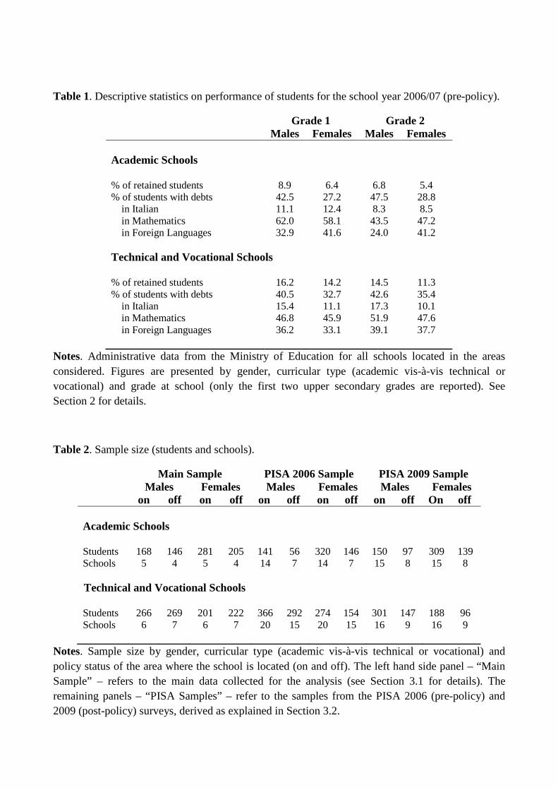
Table 1. Descriptive statistics on performance of students for the school year 2006/07 (pre-policy).
Grade 1 Grade 2 Males Females Males Females Academic Schools % of retained students 8.9 6.4 6.8 5.4 % of students with debts 42.5 27.2 47.5 28.8 in Italian 11.1 12.4 8.3 8.5 in Mathematics 62.0 58.1 43.5 47.2 in Foreign Languages 32.9 41.6 24.0 41.2 Technical and Vocational Schools % of retained students 16.2 14.2 14.5 11.3 % of students with debts 40.5 32.7 42.6 35.4 in Italian 15.4 11.1 17.3 10.1 in Mathematics 46.8 45.9 51.9 47.6 in Foreign Languages 36.2 33.1 39.1 37.7
Notes. Administrative data from the Ministry of Education for all schools located in the areas considered. Figures are presented by gender, curricular type (academic vis-à-vis technical or vocational) and grade at school (only the first two upper secondary grades are reported). See Section 2 for details.
Table 2. Sample size (students and schools).
Main Sample PISA 2006 Sample PISA 2009 Sample Males Females Males Females Males Females on off on off on off on off on off On off Academic Schools Students 168 146 281 205 141 56 320 146 150 97 309 139 Schools 5 4 5 4 14 7 14 7 15 8 15 8 Technical and Vocational Schools Students 266 269 201 222 366 292 274 154 301 147 188 96 Schools 6 7 6 7 20 15 20 15 16 9 16 9
Notes. Sample size by gender, curricular type (academic vis-à-vis technical or vocational) and policy status of the area where the school is located (on and off). The left hand side panel – “Main Sample” – refers to the main data collected for the analysis (see Section 3.1 for details). The remaining panels – “PISA Samples” – refer to the samples from the PISA 2006 (pre-policy) and 2009 (post-policy) surveys, derived as explained in Section 3.2.
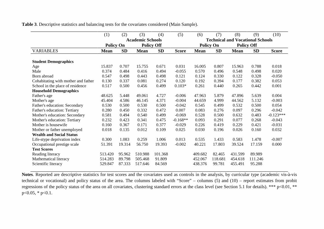
Table 3. Descriptive statistics and balancing tests for the covariates considered (Main Sample).
(1) (2) (3) (4) (5) (6) (7) (8) (9) (10) Academic Schools Technical and Vocational Schools Policy On Policy Off Policy On Policy Off VARIABLES Mean SD Mean SD Score Mean SD Mean SD Score Student Demographics Age 15.837 0.707 15.755 0.671 0.031 16.005 0.807 15.963 0.788 0.018 Male 0.374 0.484 0.416 0.494 -0.055 0.570 0.496 0.548 0.498 0.020 Born abroad 0.547 0.498 0.443 0.498 0.121 0.124 0.330 0.122 0.328 -0.050 Cohabitating with mother and father 0.130 0.337 0.081 0.274 0.120 0.192 0.394 0.177 0.382 0.053 School in the place of residence 0.517 0.500 0.456 0.499 0.103* 0.261 0.440 0.265 0.442 0.001 Household Demographics Father's age 48.625 5.448 49.061 4.727 -0.006 47.963 5.879 47.896 5.639 0.004 Mother's age 45.404 4.586 46.145 4.371 -0.004 44.659 4.999 44.562 5.132 -0.003 Father's education: Secondary 0.530 0.500 0.530 0.500 -0.042 0.545 0.499 0.532 0.500 0.054 Father's education: Tertiary 0.280 0.450 0.332 0.472 0.007 0.083 0.276 0.097 0.296 -0.042 Mother's education: Secondary 0.581 0.494 0.540 0.499 -0.069 0.528 0.500 0.632 0.483 -0.123*** Mother's education: Tertiary 0.232 0.423 0.341 0.475 -0.168** 0.093 0.291 0.077 0.268 -0.043 Mother is housewife 0.160 0.367 0.171 0.377 -0.029 0.226 0.419 0.229 0.421 -0.031 Mother or father unemployed 0.018 0.135 0.012 0.109 0.025 0.030 0.196 0.026 0.160 0.032 Wealth and Social Status Life-stype deprivation index 0.300 1.083 0.259 1.006 0.013 0.535 1.433 0.583 1.478 -0.007 Occupational prestige scale 51.391 19.314 56.750 19.393 -0.002 40.221 17.803 39.524 17.159 0.000 Test Scores Reading literacy 513.420 95.962 510.988 101.368 409.682 82.465 431.599 89.989 Mathematical literacy 514.283 89.798 505.468 91.809 452.067 118.681 454.618 111.246 Scientific literacy 529.847 87.333 517.646 84.569 438.376 99.781 455.491 95.288
Notes. Reported are descriptive statistics for test scores and the covariates used as controls in the analysis, by curricular type (academic vis-à-vis technical or vocational) and policy status of the area. The columns labeled with “Score” – columns (5) and (10) – report estimates from probit regressions of the policy status of the area on all covariates, clustering standard errors at the class level (see Section 5.1 for details). *** p<0.01, ** p<0.05, * p<0.1.

Table 4. Descriptive statistics for test scores (Main Sample).
Males Females On Off On Off Academic Schools Reading Mean 500.670 509.438 521.042 512.092 SD 91.090 102.069 98.128 101.102 Math Mean 540.312 523.952 498.814 492.304 SD 79.690 91.804 91.999 89.734 Science Mean 545.119 523.044 520.717 513.828 SD 86.278 83.872 86.833 85.055 Technical and Vocational Schools Reading Mean 411.271 418.770 407.558 447.144 SD 80.488 85.151 85.194 93.376 Math Mean 480.705 484.796 413.787 417.886 SD 113.330 96.482 115.081 117.043 Science Mean 453.240 460.934 418.407 448.835 SD 104.739 101.633 89.128 86.668
Notes. Summary statistics by gender, curricular type (academic vis-à-vis technical or vocational) and policy status of the area where the school is located (on and off).
Table 5. Average effects for achievement (Main Sample).
Reading Mathematics Science (1) (2) (3) (4) (5) (6) Males Females Males Females Males Females Academic Schools -18.5915 17.4019 5.6371 6.2289 16.9269 11.0727 (12.072) (13.764) (11.995) (11.551) (12.031) (9.193) Technical and Vocational Schools 2.3689 -39.5927 -7.956 -1.3815 -0.4246 -38.5546 (10.961) (11.561) (14.854) (12.718) (12.957) (11.688)
Notes. Results were obtained from separate regressions by gender and curricular type (academic vis-à-vis technical or vocational). All regressions include as controls the variables in Table 3. Robust standard errors clustered at the class level are reported in parentheses.
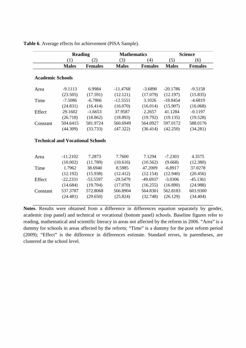
Table 6. Average effects for achievement (PISA Sample).
Reading Mathematics Science (1) (2) (3) (4) (5) (6) Males Females Males Females Males Females Academic Schools Area -9.1113 6.9984 -11.4768 -3.6890 -20.1786 -9.5158 (23.505) (17.591) (12.121) (17.079) (12.197) (15.835) Time -7.5086 -6.7866 -12.5551 3.1026 -18.8454 -4.6819 (24.831) (16.414) (16.070) (16.014) (15.907) (16.068) Effect 29.1602 -1.6653 37.9587 2.2657 41.1284 -0.1197 (26.718) (18.862) (18.893) (19.792) (19.135) (19.528) Constant 504.6415 581.9724 560.6949 564.0927 597.0172 588.0176 (44.309) (33.733) (47.322) (36.414) (42.250) (34.281) Technical and Vocational Schools
Area -11.2102 7.2873 7.7600 7.1294 -7.2303 4.3575 (10.002) (11.789) (10.616) (10.562) (9.668) (12.380) Time 1.7962 38.6940 8.5985 47.2009 -6.8917 37.0278 (12.192) (15.938) (12.412) (12.154) (12.940) (20.456) Effect -22.2331 -53.5597 -29.5479 -49.6937 -3.0306 -45.1361 (14.684) (19.704) (17.070) (16.255) (16.890) (24.988) Constant 537.3787 572.8068 566.8904 564.8301 562.8183 603.9300 (24.481) (29.650) (25.824) (32.748) (26.129) (34.404)
Notes. Results were obtained from a difference in differences equation separately by gender, academic (top panel) and technical or vocational (bottom panel) schools. Baseline figures refer to reading, mathematical and scientific literacy in areas not affected by the reform in 2006. “Area” is a dummy for schools in areas affected by the reform; “Time” is a dummy for the post reform period (2009); “Effect” is the difference in differences estimate. Standard errors, in parentheses, are clustered at the school level.
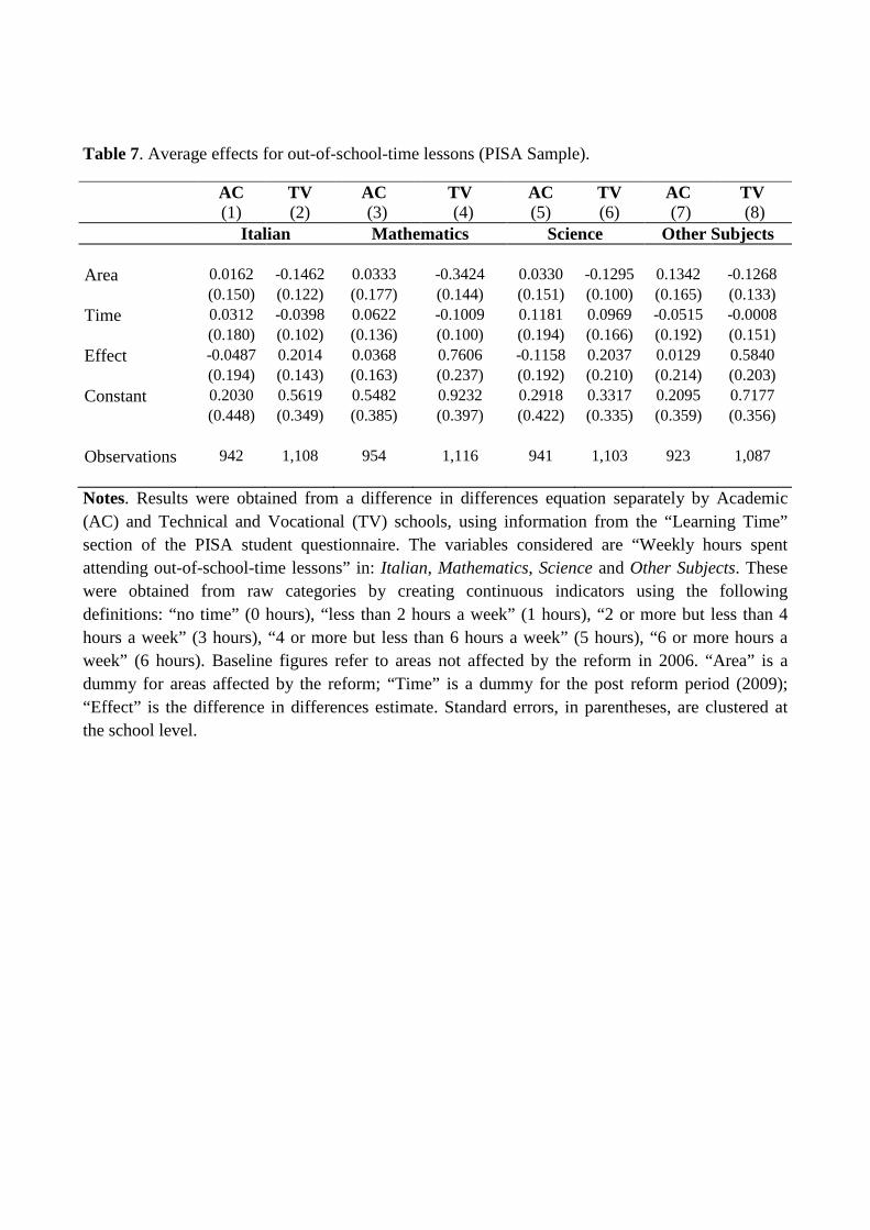
Table 7. Average effects for out-of-school-time lessons (PISA Sample).
AC TV AC TV AC TV AC TV (1) (2) (3) (4) (5) (6) (7) (8) Italian Mathematics Science Other Subjects Area 0.0162 -0.1462 0.0333 -0.3424 0.0330 -0.1295 0.1342 -0.1268 (0.150) (0.122) (0.177) (0.144) (0.151) (0.100) (0.165) (0.133) Time 0.0312 -0.0398 0.0622 -0.1009 0.1181 0.0969 -0.0515 -0.0008 (0.180) (0.102) (0.136) (0.100) (0.194) (0.166) (0.192) (0.151) Effect -0.0487 0.2014 0.0368 0.7606 -0.1158 0.2037 0.0129 0.5840 (0.194) (0.143) (0.163) (0.237) (0.192) (0.210) (0.214) (0.203) Constant 0.2030 0.5619 0.5482 0.9232 0.2918 0.3317 0.2095 0.7177 (0.448) (0.349) (0.385) (0.397) (0.422) (0.335) (0.359) (0.356) Observations 942 1,108 954 1,116 941 1,103 923 1,087 Notes. Results were obtained from a difference in differences equation separately by Academic (AC) and Technical and Vocational (TV) schools, using information from the “Learning Time” section of the PISA student questionnaire. The variables considered are “Weekly hours spent attending out-of-school-time lessons” in: Italian, Mathematics, Science and Other Subjects. These were obtained from raw categories by creating continuous indicators using the following definitions: “no time” (0 hours), “less than 2 hours a week” (1 hours), “2 or more but less than 4 hours a week” (3 hours), “4 or more but less than 6 hours a week” (5 hours), “6 or more hours a week” (6 hours). Baseline figures refer to areas not affected by the reform in 2006. “Area” is a dummy for areas affected by the reform; “Time” is a dummy for the post reform period (2009); “Effect” is the difference in differences estimate. Standard errors, in parentheses, are clustered at the school level.

Table 8. Effects for retention and promotion rates (administrative data).
Academic Schools Technical Schools Vocational Schools (1) (2) (3) (4) (5) (6) (7) (8) (9) In June Admitted Retained In June Admitted Retained In June Admitted Retained Effect Grade 1 0.0473 0.0526 0.0112 0.0657 0.0398 0.0506 0.0143 -0.0405 0.0899 (0.030) (0.034) (0.012) (0.020) (0.019) (0.017) (0.065) (0.079) (0.047) Effect Grade 2 0.0560 0.0566 0.0161 0.0680 0.0571 0.0381 0.0083 -0.0204 0.0625 (0.029) (0.033) (0.010) (0.021) (0.020) (0.017) (0.068) (0.081) (0.049) Effect Grade 3 0.0375 0.0400 0.0164 0.0507 0.0485 0.0333 (0.029) (0.033) (0.009) (0.020) (0.020) (0.016) Effect Grade 4 0.0374 0.0387 0.0123 0.0448 0.0376 0.0294 0.0137 -0.0436 0.0962 (0.030) (0.032) (0.008) (0.020) (0.017) (0.015) (0.068) (0.083) (0.049) Grade 2 -0.0312 -0.0004 -0.0309 -0.0315 0.0132 -0.0449 -0.0357 0.0181 -0.0534 (0.011) (0.012) (0.005) (0.009) (0.010) (0.008) (0.011) (0.012) (0.010) Grade 3 -0.0116 0.0086 -0.0204 -0.0371 -0.0031 -0.0341 (0.011) (0.014) (0.007) (0.010) (0.012) (0.011) Grade 4 -0.0017 0.0459 -0.0482 -0.0430 0.0330 -0.0763 -0.0503 0.0555 -0.1053 (0.015) (0.017) (0.007) (0.011) (0.015) (0.011) (0.019) (0.016) (0.016) Enrolment 0.0001 -0.0000 0.0001* -0.0001 -0.0005 0.0004 -0.0000 -0.0003 0.0003 (0.000) (0.000) (0.000) (0.000) (0.000) (0.000) (0.000) (0.000) (0.000) Constant 0.6876 0.6119 0.0774 0.6333 0.4867 0.1471 0.5742 0.3625 0.2083 (0.021) (0.023) (0.010) (0.014) (0.022) (0.016) (0.020) (0.020) (0.022) Observations 1,092 1,092 1,092 1,415 1,415 1,415 800 800 800
Notes. Reported are estimates of the ATE obtained from school fixed effects equations, by curricular type, using administrative data granted by the Italian Ministry of Education and local agencies. The available data refer to school grades, for the years 2006/07 (pre-reform), 2007/08, 2008/09 and 2019/10 (post-reform). Columns (1), (4) and (7) refer to students whose final status (retention or promotion to the next grade) is determined in June. Columns (2), (5) and (8) refer to students admitted to the next grade in June. Columns (3), (6) and (9) report the overall retention rates at the end of the school year, computed by considering retention in June or after the remedial exam in September. Standard errors, in parentheses, are clustered by school.

Figure 1. Quantile treatment effects for achievement (Main Sample).
Academic Schools
Technical and Vocational Schools
Notes. Reported are estimates of quantile regressions for reading, mathematical and scientific literacy. Results were obtained from separate regressions by gender and curricular type (academic vis-à-vis technical or vocational). All regressions control for variables in Table 3, as explained in Section 4. Bootstrap standard errors based on 200 replications and clustered at the class level are used to compute 95% confidence intervals.
-100
-50
050
0 50 100 0 50 100
Females Males
Graphs by gender
Reading
-100
-50
050
0 50 100 0 50 100
Females Males
Graphs by gender
Reading
-50
050
100
0 50 100 0 50 100
Females Males
Graphs by gender
Math
-100
-50
050
0 50 100 0 50 100
Females Males
Graphs by gender
Math
-50
050
100
0 50 100 0 50 100
Females Males
Graphs by gender
Science
-100
-50
050
100
0 50 100 0 50 100
Females Males
Graphs by gender
Science

Figure 2. Retention rates by cohort of birth (1994 reform).
Notes. Reported are profiles for retention rates by cohort of enrollment at upper secondary school (e.g. 78 stands for “born in 1978” and enrolled at age 14), separately for the first four school grades. Only regions in the Northern/Central part of Italy are considered. The reform year is marked with the red dot. Source: ISTAT (Italian National Bureau of Statistics, before the school year 1997/98) and MIUR (Ministry of Education, from the school year 1998/99).
0.0
5.1
.15
.2.2
5.3
71 73 75 77 79 81 83 85 87 71 73 75 77 79 81 83 85 87
Vocational Schools Academic Schools
Grade 1 Grade 2Grade 3 Grade 4
Year of birth at entrance
Graphs by School type
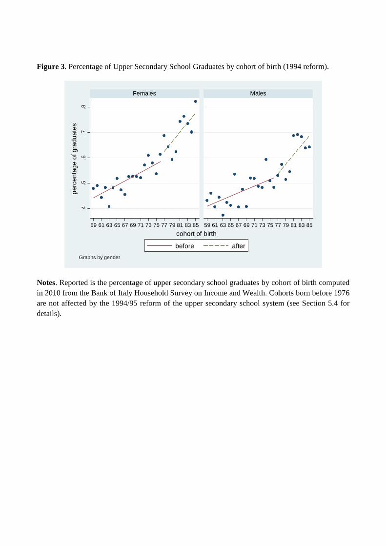
Figure 3. Percentage of Upper Secondary School Graduates by cohort of birth (1994 reform).
Notes. Reported is the percentage of upper secondary school graduates by cohort of birth computed in 2010 from the Bank of Italy Household Survey on Income and Wealth. Cohorts born before 1976 are not affected by the 1994/95 reform of the upper secondary school system (see Section 5.4 for details).
.4.5
.6.7
.8
59 61 63 65 67 69 71 73 75 77 79 81 83 85 59 61 63 65 67 69 71 73 75 77 79 81 83 85
Females Males
before after
perc
enta
ge o
f gra
duat
es
cohort of birth
Graphs by gender

Appendix

Table A.1. Average effects for achievement (sensitivity analysis - Main Sample).
Academic Schools Reading Mathematics Science Males Females Males Females Males Females Effect -20.6359 19.2969 -0.1515 7.2619 14.5582 11.1516 (15.5322) (13.0739) (14.5347) (11.9800) (16.4977) (8.7610) Baseline 521.3540 505.7525 532.5818 491.2104 528.2151 512.9147 (12.6388) (7.8504) (11.3752) (6.9062) (11.7942) (7.1733) Technical and Vocational Schools Reading Mathematics Science Males Females Males Females Males Females Effect 3.1842 -44.9988 -3.6869 -6.8148 -0.5680 -43.9076 (14.4280) (12.9602) (18.9895) (18.3495) (17.5347) (13.8951) Baseline 415.6732 447.7098 481.5509 423.1282 459.6394 455.3818 (10.8549) (9.7333) (16.4587) (14.8501) (13.6718) (9.8758)
Notes. Results were obtained from separate groups defined by gender and curricular type (academic and technical or vocational), using the propensity score weighting estimator described in Imbens (2004). Baseline figures refer to reading, mathematical and scientific literacy in areas not affected by the reform. Standard errors, in parentheses, were computed via bootstrap using 200 replications, allowing for clustering at the class level.
Table A.2. Average effects for achievement (sensitivity analysis - Main Sample).
Reading Mathematics Science (1) (2) (3) (4) (5) (6) Males Females Males Females Males Females Academic Schools -26.0238 1.7277 2.5943 -3.7520 10.3944 -0.0456 (7.2362) (8.6828) (9.0698) (6.9193) (7.8627) (6.5460) Technical and Vocational Schools -0.1710 -22.6390 -11.8815 22.5778 -3.0561 -21.1343 (7.7645) (6.6710) (9.2264) (9.4210) (8.8225) (6.7858)
Notes. Results were obtained from separate regressions by gender and curricular type (academic vis-à-vis technical or vocational). All regressions include as controls the variables in Table 3, and a proxy for student’s ability obtained as explained in Section 5.2. Robust standard errors clustered at the class level are reported in parentheses.

Table A.3. Average effects for family inputs (PISA Sample).
AC TV AC TV AC TV AC TV (1) (2) (3) (4) (5) (6) (7) (8) Methods Discipline Education Progress Area -0.0555 -0.0470 -0.0439 0.0528 0.0332 0.0477 -0.0343 0.0562 (0.058) (0.035) (0.032) (0.036) (0.052) (0.038) (0.063) (0.055) Time -0.0431 -0.0875 -0.0815 -0.0021 -0.0064 -0.0514 0.0140 0.0023 (0.052) (0.030) (0.031) (0.039) (0.047) (0.037) (0.042) (0.068) Effect 0.0397 0.0533 0.0817 -0.0473 0.0034 0.0280 -0.0462 -0.0271 (0.058) (0.042) (0.039) (0.044) (0.058) (0.043) (0.052) (0.077) Constant 0.8927 0.9016 0.8930 0.8332 0.6909 0.8930 0.7886 0.7469 (0.113) (0.104) (0.092) (0.107) (0.132) (0.093) (0.116) (0.117) Observations 1,008 1,186 1,017 1,191 1,006 1,189 1,014 1,193
AC TV (9) (10) Spending Area 26.9392 -8.6224 (24.338) (10.650) Time -23.5837 -37.9330 (22.939) (16.156) Effect -18.5209 9.9809 (26.098) (21.791) Constant 209.0503 202.209 (55.470) (40.018) Observations 1,013 1,164
Notes. Results were obtained from a difference in differences equation, by Academic (AC) and Technical and Vocational (TV) schools, using information from the PISA parent questionnaire. The variables considered are: “I am happy with the content taught and the instructional methods used in my child’s school” (Methods, columns (1)-(2), dummy for agree or strongly agree); “I am satisfied with the disciplinary atmosphere in my child’s school” (Discipline, columns (3)-(4), dummy for agree or strongly agree); “My child’s school does a good job in educating students” (Education, columns (5)-(6), dummy for agree or strongly agree); “My child’s progress is carefully monitored by the school” (Progress, columns (7)-(8), dummy for agree or strongly agree); “Education costs” (Spending, columns (9)-(10); the variable is coded by PISA using the following categories: less than 100EUR, between 100EUR and 200EUR, between 200EUR and 300EUR, between 300EUR and 400EUR, and more than 400EUR. We take as reference values for these categories 50EUR, 150EUR, 250EUR, 350EUR and 500EUR, respectively). Standard errors, in parentheses, are clustered at the school level.
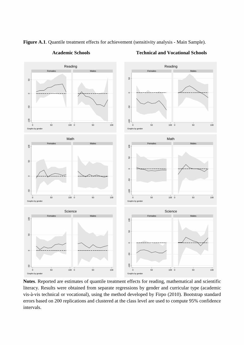
Figure A.1. Quantile treatment effects for achievement (sensitivity analysis - Main Sample).
Academic Schools
Technical and Vocational Schools
Notes. Reported are estimates of quantile treatment effects for reading, mathematical and scientific literacy. Results were obtained from separate regressions by gender and curricular type (academic vis-à-vis technical or vocational), using the method developed by Firpo (2010). Bootstrap standard errors based on 200 replications and clustered at the class level are used to compute 95% confidence intervals.
-100
-50
050
0 50 100 0 50 100
Females Males
Graphs by gender
Reading
-100
-50
050
0 50 100 0 50 100
Females Males
Graphs by gender
Reading
-50
050
100
0 50 100 0 50 100
Females Males
Graphs by gender
Math
-100
-50
050
100
0 50 100 0 50 100
Females Males
Graphs by gender
Math
-50
050
100
0 50 100 0 50 100
Females Males
Graphs by gender
Science
-100
-50
050
100
0 50 100 0 50 100
Females Males
Graphs by gender
Science
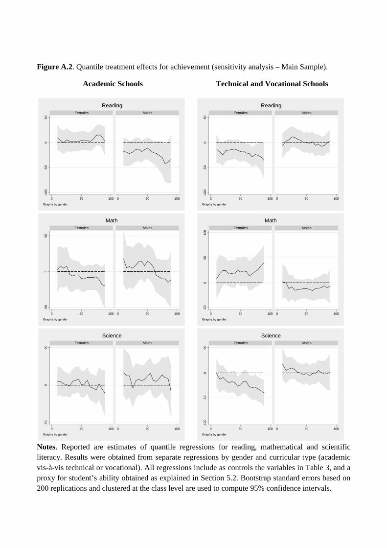
Figure A.2. Quantile treatment effects for achievement (sensitivity analysis – Main Sample).
Academic Schools
Technical and Vocational Schools
Notes. Reported are estimates of quantile regressions for reading, mathematical and scientific literacy. Results were obtained from separate regressions by gender and curricular type (academic vis-à-vis technical or vocational). All regressions include as controls the variables in Table 3, and a proxy for student’s ability obtained as explained in Section 5.2. Bootstrap standard errors based on 200 replications and clustered at the class level are used to compute 95% confidence intervals.
-100
-50
050
0 50 100 0 50 100
Females Males
Graphs by gender
Reading
-100
-50
050
0 50 100 0 50 100
Females Males
Graphs by gender
Reading
-50
050
0 50 100 0 50 100
Females Males
Graphs by gender
Math
-50
050
100
0 50 100 0 50 100
Females Males
Graphs by gender
Math
-50
050
0 50 100 0 50 100
Females Males
Graphs by gender
Science
-100
-50
050
0 50 100 0 50 100
Females Males
Graphs by gender
Science

Figure A.3. Classification of Italian provinces depending on policy status and survey design.
Notes. The province of Trento (Northern Italy, in light blue) is the only province not affected by the reform. An Italian province is a territory administratively similar to a US county. Provinces in dark blue are used as donors in the evaluation design to match schools in the province of Trento to similar schools outside its administrative border. All remaining provinces are discarded from the analysis. See Section 3 for additional details.
TRENTO
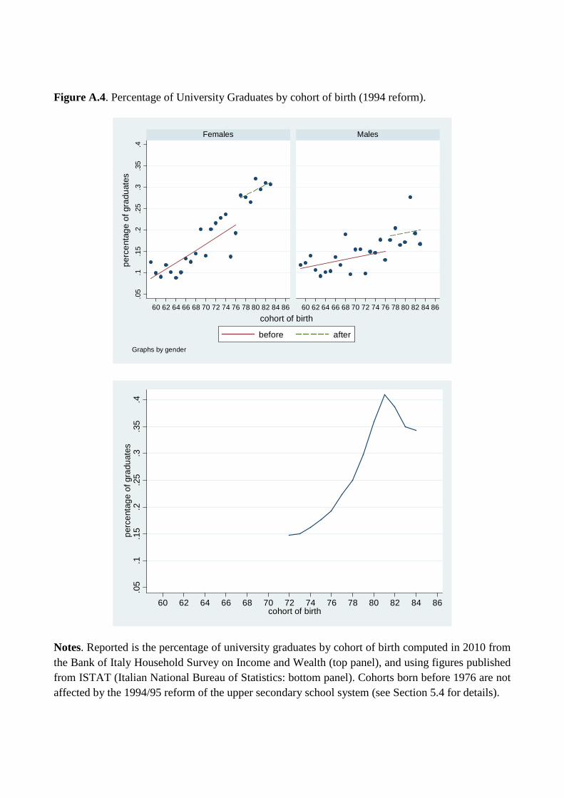
Figure A.4. Percentage of University Graduates by cohort of birth (1994 reform).
Notes. Reported is the percentage of university graduates by cohort of birth computed in 2010 from the Bank of Italy Household Survey on Income and Wealth (top panel), and using figures published from ISTAT (Italian National Bureau of Statistics: bottom panel). Cohorts born before 1976 are not affected by the 1994/95 reform of the upper secondary school system (see Section 5.4 for details).
.05
.1.1
5.2
.25
.3.3
5.4
60 62 64 66 68 70 72 74 76 78 80 82 84 86 60 62 64 66 68 70 72 74 76 78 80 82 84 86
Females Males
before after
perc
enta
ge o
f gra
duat
es
cohort of birth
Graphs by gender
.05
.1.1
5.2
.25
.3.3
5.4
perc
enta
ge o
f gra
duat
es
60 62 64 66 68 70 72 74 76 78 80 82 84 86cohort of birth