theory of computing - gunma u
TRANSCRIPT

Theory of Computing
April 6, 2017
1 Preliminaries (Mainly for graph)
1.1 Notation
Let G = (V,E) be a graph.
1. V (G) and E(G) denote the vertex set and the edge set of G, respectively, i.e., V = V (G),E = E(G).
2. For W ⊆ V , G[W ] denotes the indeuced subgraph of G by W .
3. For v ∈ V , degG(v) (or simply deg(v)) denotes the degree of v. ∆(G) denotes the maximumdegree in G.
4. For v ∈ V , NG(v) (or simply N(v)) denotes the verices adjacent to v, i.e., NG(v) = {u |{u, v} ∈ E}.
5. E denotes the complement of E, i.e., {{u, v} | {u, v} ̸∈ E}. The graph (V,E), denoted byG, is called the complement graph of G
1.2 Graph parameters
1.2.1 Graph parameters based on vertex subset
Let G be a graph and let W ⊆ V (G).
Independent Set
• W is an independent set (of G) if {u, v} ̸∈ E(G) for all u, v ∈ W .
• An independent set X (of G) is called maximum if there is no independent set Y (of G) suchthat |X| < |Y |.
• The independence number of G, denoted by α(G), is the size of maximum independent setof G
1
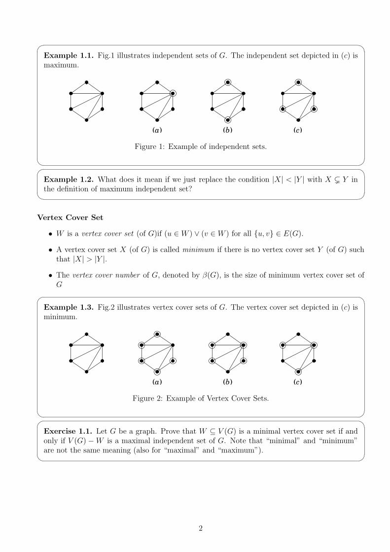
� �Example 1.1. Fig.1 illustrates independent sets of G. The independent set depicted in (c) ismaximum.
(a) (b) (c)
Figure 1: Example of independent sets.
� �� �Example 1.2. What does it mean if we just replace the condition |X| < |Y | with X ⊊ Y inthe definition of maximum independent set?� �
Vertex Cover Set
• W is a vertex cover set (of G)if (u ∈ W ) ∨ (v ∈ W ) for all {u, v} ∈ E(G).
• A vertex cover set X (of G) is called minimum if there is no vertex cover set Y (of G) suchthat |X| > |Y |.
• The vertex cover number of G, denoted by β(G), is the size of minimum vertex cover set ofG� �
Example 1.3. Fig.2 illustrates vertex cover sets of G. The vertex cover set depicted in (c) isminimum.
(a) (b) (c)
Figure 2: Example of Vertex Cover Sets.
� �� �Exercise 1.1. Let G be a graph. Prove that W ⊆ V (G) is a minimal vertex cover set if andonly if V (G) −W is a maximal independent set of G. Note that “minimal” and “minimum”are not the same meaning (also for “maximal” and “maximum”).� �
2

2 Class NP and NP-completeness
2.1 What does “problem” mean ?: Problem and Instance
• We should distinguish between “Problem” and “Instance”.
• Formally “problem” considered here can be viewed as recognition problem: for a fixed set(language) L and any elemnt (string) s, decide whether s ∈ L or not, where an elementcorresponds an input.
• In the formal definition, “problem” described in natural language is translated into an arti-ficial language (usually a Turing machine).
� �Example 2.1. Difference between “problem” and “instance”:
• Problem: given a graph G and a positive integer k, Does G have a vertex cover set ofsize at most k ?
• Instance: The graph illustrated in Fig. 2 and k = 3.
• The graph illustrated in Fig. 2 is an yes instance for k ≥ 3, and no instance for k ≤ 2.
• Let VCP denote the set {(G, k) | (G, k) is an yes instance on VC}. Then, “Vertex CoverProblem” can be viewed as the recognition problem: Decide wherther or not (G, k) ∈V CP for a given input(G, k),� �
2.2 How to measure the difficulty of a problem (in the sense of com-putation)?
feeling (subjective measure) Not Goodmathematics (objective measure) Good → function is used usually
Computational complexityDifficult/Easy: problems which require much/less resources (time, space)
2.3 Types of problems
2.3.1 Optimization Problem
• Solution space: A space containing all solutions
• Objective function: A function from solution space (or the set of all solutions) to the set ofreal numbers
• Objective value: The value of the objective function at a point
• Constraint: Conditions, Restrictions
• Feasible solution: A solution subject to the constraint conditions
• Optimal solution: The best solution of feasible solutions (not necessarily unique solution)
3

• Optimal value: The value of optimal solutions (the optimal value is of course unique)
• Optimization problem (Decision version): Computing the optimal value.
• Optimization problem (Construction version): Finding an optimal solution.
Solution Space
Feasible Solutions
Opt. Sol.value 5
Opt. Val 3 value 2value 4(a)
(c)
(b)
(d)
Graph G
Figure 3: Optimization problem, feasible solutions, optimal solution
� �Example 2.2. Example of optimization problem: VC
• Solution space: {U | U ⊆ V (G)}
• Objective function: U 7→ |U |
• Constraint: U must be vertex cover of G
• Feasible solution: {U | U :vertex cover}
• Optimal solution: A minimum vertex cover set
• Optimal value: The size of minimum (optimal) vertex cover set, i.e., β(G).
• Optimization problem: Input: a graph GOutput: β(G)� �
2.3.2 Decision Problem
• Problem for which we can answer with “yes” or “no”.
� �Example 2.3. Example of decision problem: VCInput: a graph G and a positive integer k
Output:
{yes if β(G) ≤ kno otherwise� �
2.3.3 Construction Problem
• Problem for which we have to answer with “yes + additional information” or “no”, whereadditional information is a proof or evidence showing that the input is indeed an “yes in-stance”.
4

� �Example 2.4. Example of construction problem: VCInput: a graph G and a positive integer k
Output:
{yes + a vertex cover set of size at most k if β(G) ≤ kno otherwise� �
2.3.4 Verification Problem
• Input: a proof or evidence
Output:
{yes if the proof is validno otherwise� �
Example 2.5. Example of verification problem: VCInput: a graph G and U ⊆ V (G)
Output:
{yes if U is a vertex cover set of Gno otherwise� �
2.4 Polynomial time computable
In the theoretical analysis of algorithms, for theoretical estimation of the running time, we oftentake the following way:
• quantification of its input size, e.g., g : Input 7→ N
• estimatation of running cost as a function on input size, e.g., f : N 7→ N .� �Example 2.6. Example on VC:
• For a given graph G, the size of G is usually defined as its cardinality of the vertex set|V (G)|.
• Let us use the symbol n to indicate the size of G. Then, the running time for the followingnaive algorithm for VC can be represented as O(2n).
Procedure FindMinimumVCInput: a graph G = (V,E)Output: a minimum vertex cover set of G1: i := 1;2: while i ≤ n− 1 do3: foreach U ⊆ V (G) of size i do4: go to step 8 if U is a vertex cover set;5: od;6: i := i+1;7: od;8: output the vertex cover set of size i and stop;� �
• A problem is polynomial time solvable if there is an algorithm with running time O(f(p)),where f is a polynomial multi valued function on p.
5

• In the theoretical analysis, if a problem A is polynomial time solvable, then A is referred toas easy, and if not as hard.
2.5 Misc.
• Is there any difference between decision version and construction version in optimizationproblem ?
• If there is, which problem is more difficult than the other ?
• For NP-complete problems P , there is essentially no difference between decision versionand construction version in optimization problem on P . (See “Complexity and Approxima-tion: Combinatorial Optimization Problems and Their Approximability Properties” by P.Crescenzi, G. Gambosi, V. Kann, A. Marchetti-Spaccamela, M. Protasi, G. Ausiello)
2.6 Class NP
Class of decision problems satisfying the following:
1. every yes instance has a short proof (“Short” means poly. size or poly. time).
2. each short proof can be checked in poly. time
• If a problem A is in NP, I is an yes instance of A iff there exists a short proof (evidence)confirming that I is indeed yes instance.
• For example, the problem to decide whether β(G) ≤ k or not for a given graph G and positiveinteger k, is in NP.Because β(G) can be considered as a short proof for each yes instance of the problem.
• The point is that for problems in NP we do not care about the cost of finding the short proof.We only care about the cost of verification.
2.7 Find vs. Verify
Consider the following:
• There are twins Mana and Kana who have the same mathematical ability.
• Suppose that Mana can verify the correctness of a proof for a mathematical theorem.
• Then, How do you think the following claim?Claim: Kana should be able to prove the mathematical theorem, because Mana can verifythe proof and Kana has the same mathematical ability as Mana’s ability.
2.8 Problems for which no poly. time algorithms are known (NP-complete problem)
• “Hard problems” means problems for which there seems to be no poly. time algorithm.
• Why “seems”? Many researchers have tried to prove that there is no poly. time algorithmfor those problems, but still unproved.
6

• There are, however, some research progress: If one of problems called NP-complete can besolved in poly. time, any problem in class NP also can be solved in poly. time.
• Famous examples of NP-complete problems are: Independet set problem, Vertex cover prob-lem, Hamiltonian cycle problem, Traveling sales-person problem (those all problems aredecision problems) (See Fig. 4).
Vertex Cover Problem Hamiltonian Cycle Problem
Traveling Sales-person Problem Graph Coloring Problem
Matching
Minimum Spaning Tree Problem
Shortest Path Problem
. . .
Class NP
NP-Complete Problems
Class P
Figure 4: Class NP, Class P, NP-complete
� �Exercise 2.1. Let β(G) denote the minimum number of vertices which covers all edges in agraph G. Is the following problem in NP: Given a graph G and an integer k, decide whetheror not β(G) > k.� �� �Exercise 2.2. There is a dormitory which can have 100 students. But there are 400 studentswho want to enter the dormitory. And we have a list of pair of students who are on bad terms.So we have to choose 100 students from the 400 students so as to there is no pair in the 100students who are on bad terms. How to describe the above problem in terms of graph theory?� �� �Exercise 2.3. Show that if one of the decision problem for vertex cover problem and thedecision problem for independent set problem can be solved in polynomial time, then the otherproblem also can be solved in polynomial time.� �
7

3 Reduction
• Is it possible to compare two problems? For example, which problem is computationallyharder, Hamiltonian cycle problem and vertex cover problem?
• It would be nice if we can have a partial order ≤ such that A ≤ B if A is not harder than B.
• Let A and B are problems. Intuitively speaking, we will write A ≤P B if B can be solved inpoly. time, then A can also be solved in poly. time.
• The idea how to get such a partial order is to assume that we have a subroutine solving Bin poly. time, and to use it for solving A as a black box.
• Cook reduction vs. Karp reduction (SAT ≤p SAT ?).
� �Definition 3.1. Let A and B are problems, and f be a polynomial time algorithm whichtransforms an instance of A to an instance of B. A is called reducible to B if x is an yesinstance of A iff f(x) is an yes instance of B. We write A ≤P B.� �Intuitively, solving A can be changed into solving B with keeping yes instances.
3.1 VCP vs. HCP� �Theorem 3.1. If Hamiltonian cycle problem can be solved in poly. time, then and vertexcover problem can also be solved in poly. time. That is, VCP ≤P HCP.� �
Proof We first show the construction of G′.
Construction of G′
1. The idea here is to construct a graph G′ with the following property from given G and k asan instance of VC in poly. time.
Property G has a vertex cover set of size kiff⇐⇒ G′ has a Hamiltonian cycle.
2. If HCP can be solved in poly. time, then VCP can also be solved in poly. time. SO we canprove the theorem (See Fig.5).
Graph GPositiveinteger k
Graph G’YES
NO
Transform in poly. time Solve in poly. time
Algorithm solving VCP
Algorithm solving HCP YES
NO
Figure 5: Scheme of reduction
8

3. How to construct? Recall that from given G and k, we will construct a graph G′.
4. First, for each {u, v} ∈ E(G), construct a graph G{u,v} as shown in Fig.6.
u
v
enter
enter
u
v
u
v
u
v
(a) (b) (c)
exit
exit
Graph G{u,v}
{u,v}
Figure 6: Graph G{u,v}
� �Proposition 3.2. In each graph G{u,v}, it is necessary one or two paths to visite all thevertices in G (without revisit) by the paths with “enter” and “exit” as the end points.
Each graph G{u,v} has the following property:
1. Case where one path is enough:
1. visite, starting from u, in the way illustrated in Fig. 6 (a), (*)
2. visite, starting from v, in the way illustrated in Fig. 6 (b), (**)
2. Case where two path are required:
1. the path starting from u consists of the upper half vertices, and the pathstarting from v consists of the lower half vertices (See 6 (c), (***) ).
3. There is no other way to visite the all vertices in G.
The above property corresponds to: in a vertex cover set, each edge {u, v} is covered by:
1. only u (corresponding to (*) )
2. only v (corresponding to (**) )
3. both u and v (corresponding to (***) )� �5. Eventually, the graph G′ is constructed from the graphs G{u,v} and k vertices {a1, . . . , ak}
called transfer (or connection) by connecting those vertices (See Fig.7). Intuitively, thetransfer vertices correspond to vertex cover set of G.
9

v1
v2
v3
v6
v5
v4
{v1,v6}
{v2,v3}
{v2,v4}
{v2,v6}
{v5,v6}
{v1,v2}
{v3,v4}{v4,v5}
{v2,v5}
1
2
6
2
2
5
2
4
2
3
1
6
3
4
5
4
6
5
{v1,v6}
{v2,v3}
{v2,v4}
{v2,v6}
{v5,v6}
{v1,v2}
{v3,v4}{v4,v5}
{v2,v5}
1
2
6
2
2
5
2
4
2
3
1
6
3
4
5
4
6
5
p.p for v1
a1
. . .
ak
......
k
Inputs
Graph G’
constructed from the information of G k vertices
Figure 7: Construction of G
6. For the construction of G′ we need paths called pseudo-path: For each vertex u, make apseudo-path in the following way:
• sort the edges incident to u,{{u, vi1}, {u, vi2}, . . . , {u, videg(v)}
}in any order.
• make a path by connecting “enter” and “exit” of those edges alternatively in that order.as shown Fig.8.
• For example in Fig.8, for v4, the edges incident to v4 is {{v2, v4}, {v3, v4}, {v4, v5}}, andthe pseudo-path for v4 is made in the order {v3, v4}, {v2, v4}, {v4, v5}.• The entrance of G{v3,v4} will be referred to as the entrance of the pseudo-path for v4and the exit of G{v4,v5} will be referred to as the exit of the pseudo-path for v4.
{v1,v6}
{v2,v3}
{v2,v4}
{v2,v6}
{v5,v6}
{v1,v2}
{v3,v4}{v4,v5}
{v2,v5}
1
2
6
2
2
5
2
4
2
3
1
6
3
4
5
4
6
5
{v1,v6}
{v2,v3}
{v2,v4}
{v2,v6}
{v5,v6}
{v1,v2}
{v3,v4}{v4,v5}
{v2,v5}
1
2
6
2
2
5
2
4
2
3
1
6
3
4
5
4
6
5
{v1,v6}
{v2,v3}
{v2,v4}
{v2,v6}
{v5,v6}
{v1,v2}
{v3,v4}{v4,v5}
{v2,v5}
1
2
6
2
2
5
2
4
2
3
1
6
3
4
5
4
6
5
{v1,v6}
{v2,v3}
{v2,v4}
{v2,v6}
{v5,v6}
{v1,v2}
{v3,v4}{v4,v5}
{v2,v5}
1
2
6
2
2
5
2
4
2
3
1
6
3
4
5
4
6
5
{v1,v6}
{v2,v3}
{v2,v4}
{v2,v6}
{v5,v6}
{v1,v2}
{v3,v4}{v4,v5}
{v2,v5}
1
2
6
2
2
5
2
4
2
3
1
6
3
4
5
4
6
5
{v1,v6}
{v2,v3}
{v2,v4}
{v2,v6}
{v5,v6}
{v1,v2}
{v3,v4}{v4,v5}
{v2,v5}
1
2
6
2
2
5
2
4
2
3
1
6
3
4
5
4
6
5
p.p for v1 p.p for v3
p.p for v6
p.p for v2
p.p for v4 p.p for v5
Figure 8: Pseudo-paths
7. Next for each pseudo-path Pv (for v), connect “entrance” and “exit” of Pv to the k vertices{a1, . . . , ak} so-called transfer (See Fig.9). Recall that the transfer vertices correspond tovertex cover set of G.
10

{v1,v6} {v1,v2}1
2
1
6
{v1,v6}
{v2,v6}
{v5,v6}
6
2
1
6
6
5
. . .a1 a2 ak
. . .a1 a2 ak
. . .
Connection relation between p.p. for v1 and transfer vertices
the entrance for the psude-path
the exit for the pseudo-path
Connection relation between p.p. for v6 and transfer vertices
the entrance for the psude-path
the exit for the pseudo-path
Figure 9: Connection relation between pseudo-paths and transfers
Correctness of the construction
We now check that G′ has the following property: G has a vertex cover set of size kiff⇐⇒ G′ has
a Hamiltonian cycle.
1. From the construction, it is not difficult to see that: from the vertex cover set {v2, v4, v6} ofG, we can have a Hamiltonian cycle of G′ (see Fig.10):
1. take the entrance of pseudo-path for v2 as starting vertex,
2. after arriving the exit of pseudo-path for v2 on along the pseudo-path for v2, transferthe pseudo-path from for “v2” to “for v6” at a1, that is, move from the exit of thepseudo-path for v2 to a1, then move from a1 to the entrance of the pseudo-path for v6.
3. after arriving the exit of pseudo-path for v6 on along the pseudo-path for v6, transferthe pseudo-path from for “v6” to for “v4” at a2,
4. after arriving the exit of pseudo-path for v4 on along the pseudo-path for v4, transferthe pseudo-path from for “v4” to for “v2” at a3.
5. This description is still not enough. We need need to be careful a bit more! See G{v2,v6}for example! Actually, we have just shown the existence of a “closed walk”.
{v1,v6}
{v2,v3}
{v2,v4}
{v2,v6}
{v5,v6}
{v1,v2}
{v3,v4}{v4,v5}
{v2,v5}
{v1,v6}
{v2,v3}
{v2,v4}
{v2,v6}
{v5,v6}
{v1,v2}
{v3,v4}{v4,v5}
{v2,v5}
{v1,v6}
{v2,v3}
{v2,v4}
{v2,v6}
{v5,v6}
{v1,v2}
{v3,v4}{v4,v5}
{v2,v5}
a3
a1
a2
Transfer p.p. for v4 to p.p. for v2 at a3Transfer p.p. for v4 to p.p. for v4 at a3Transfer p.p. for v2 to p.p. for v6 at a1
Figure 10: The relation between Hamiltonian cycle and vertex cover set
2. Also for the other direction, if we can have a Hamiltonian cycle H in G′, then we can alsohave a vertex cover set of G by decomposing H into pseudo-paths and then considering forwhich vertex the pseudo-paths are.
11

3. In Fig.11, a Hamiltonian cycle in G′ is indicated by the bold line.
{v1,v6}
{v2,v3}
{v2,v4}
{v2,v6}
{v5,v6}
{v1,v2}
{v3,v4}{v4,v5}
{v2,v5}
12
62
25
24
23
1
6
34
54
65
a1
Graph G’
a2
a3
start
Figure 11: Hamiltonian cycle in G′
□� �Exercise 3.1. In Fig.11, G{v2,v4} and G{v2,v6} cover the vertices by two paths, but the otherG{v.,v.}’s cover the vertices by one path. Where does the difference come from?� �
12

4 Self-Reducible
1. Which problem is harder decision problem PD and construction problem PC for a problemP? For example, which is harder between vertex cover decision problem and vertex coverconstruction problem?
2. It is obvious, if vertex cover construction problem can be solved in poly. time, then vertexcover decision problem can also be solved in poly. time.
3. How about the other direction? Is it true that if vertex cover decision problem can be solvedin poly. time, then vertex cover construction problem can also be solved in poly. time ???
4.1 Problems on which there is no difference between decision versionand construction version� �
Theorem 4.1. Let PD be a NP-complete (decision) problem and let PC be the constructionproblem of PD. If PD can be solved in poly. time, then PC can also be solved in poly. time.� �
The proof of the above theorem is omitted, because the proof requires some knowledge of compu-tational complexity.
An example on vertex cover problem, however, is shown here. Next algorithm ConstructVCsolves vertex cover construction problem by using an algorithm solving vertex cover decision prob-lem as a subroutine. (See Fig. 12).
Procedure ConstructVCInput: graph G = (V = {v1, . . . , vn}, E), positive integer kOutput: vertex cover set of G1: U := ∅; i := 1;2: while (i ≤ n) and (G(E) ̸= ∅) do3: if G− {vi} has a vertex cover set of size k − 1 then4: begin U := U ∪ {vi}; G := G− {vi}; k := k − 1; end;5: i := i+ 1;6: od8: Output U ;
v5
グラフG
v1
v2
v3
v4
v6
v5
v1
v2
v3
v4
v6
v5
v1
v2
v3
v4
v6
v5
v1
v3
v4
v6
v5
v1
v3
v4
v6
v5
v1
v6v2v6
2頂点カバー不可能
v1
v3
v4
v6
v5
2頂点カバー可能
v4
1頂点カバー不可能
1頂点カバー可能
v5
v6
0頂点カバー不可能
v1
v6
v5
1頂点カバー可能
Figure 12: Self-reducibility for VCP
� �Exercise 4.1. Design an algorithm solving Hamiltonian cycle construction problem by usingan algorithm solving Hamiltonian cycle decision problem as a subroutine.� �
13
� �Exercise 4.2. Bandwidth problem of a graph G is to find an ordering πopt of the vertices suchthat πopt minimizes minπ max{u,v}∈E(G) |π(u) − π(v)|. Hence, an input of bandwidth decisionproblem is a pair of a graph and a positive integer, and a proof (evidence) in bandwidthconstruction problem is an ordering. Design an algorithm solving bandwidth constructionproblem by using an algorithm solving bandwidth decision problem as a subroutine.� �
4.2 Problems on which there seems to be a difference between decisionversion and construction version
1. Let n be a composite number (i.e., n is non prime number). Then there exists a pair (m, ℓ)of positive integer such that n = m× ℓ but m and ℓ both are neither 1 nor n.
2. Composite number decision problem is to determine whether n is a composite number or not,and composite number construction problem is to find a pair (m,ℓ) stated above if it is acomposite number.
3. The composite number decision problem is equivalent to prime number problem, which canbe solved in poly. time. The composite number construction problem, however, is equivalentto prime factorization, for which there is no known poly. time algorithm so far.
� �Exercise 4.3. Let A = {a1, . . . , an} be given n positve integers such that
∑ni=1 ai < 2n − 1.
Then, there exist two distinct subsets U, V ⊆ A such that∑
ai∈U ai =∑
ai∈V ai. (It, however,is not known a poly. time algorithm finding such U, V .) Prove the existence of U, V . (Hint:How many values are possible for
∑ai∈U ai ? How many subsets are there of A ?)� �
14

5 Applications of graph algorithms
5.1 Module flipping problem in VLSI
5.1.1 Module flipping problem
• We will consider here the following problem on VLSI layout. A net is a pair of terminal portsand each terminal port belongs to an individual net.
• Fig. 13 shows an example of modules and nets. In the figure, there are five modules and fivenets, and each box represents a module and has its own number. Each terminal is indicatedby a triangle with a letter a through e. The nets are represented by the five letters a throughe by twos and the two terminals with the same letter have to be connected eventually.
• For instance, the terminal d in module 1 should be linked to the terminal d in module 2.
aab
e c bd
ec
d 51 2 43
Figure 13: An example of modules and nets.
• Suppose that the layout of modules are already fixed,
• For example, in Fig.13, each module will be placed as depicted in (a) in Fig. 14.
• What we should do is to decide, for each module M , whether M should be placed withoutor with flip horizontal.
• Note here that each module can be reversed horizontally but not vertically.
• For instance, in Fig.13, we can put the five modules as illustrated in Fig. (b) or (c) in 14.
a
ab
e c
bd
ec
d
51
24
3a
ab
e c
bd
ec
d
51
24
3
(a) (b) (c)
51
24
3
Figure 14: An example of replacement with flipping.
• The problem is to find a flipping of modules so as to minimize the total length of wire toconnect terminals. We call such a minimum flipping optimal.
• For example, in Fig. 14, the total length in (b) is much larger than that in (c).
15

a
ab
e c
bd
ec
d
ab
cd
e
51
24
3a
ab
e c
bd
ec
d
ab
cd
e
51
24
3
Total wire (trace) length=15 Total wire (trace) length=4Figure 15: An example showing the difference in total length.
5.1.2 Formulation
• Let us first associate each net N with a triangle TN . TN of course has three vertices, andtwo of them are labled with the identifying numbers of the modules containing a terminal inN and the other is labled with a special label T .
• For instance, Fig. 16 illustrates a triangle associated with a that has the vertices labeledwith 3, 5, and T (Note that the terminals of T is in modules 3 and 5.)
• Furthermore, the edges in the triangle are weighted so that:For any cut C in the triangle, if only the modules in VT ̸∈ are flipped (i.e., the modules inVT∈ are not flipped), then the total length will be increased by the total weight of the cut(VT∈, VT ̸∈), . (VT∈ denotes the side (in C) containing T and VT ̸∈ the other side.
a
a
53
5 3
T
0
5-2
Net a
a
a
53
5 3
T
0
5-2
a 3
5 3
T
0
5-2
a 53
5 3
T
0
5-2
Rotate 3rd and 5th boxes 180 degrees, then the length increases 3(=-2+5).
a5
a
length 2 length 5 length 0 length 7
Rotate 5th box 180 degrees, then the length increases -2(=-2+0).
Rotate 3rd box 180 degrees, then the length increases 5(=5+0).
Figure 16: The relation between cut weight and wire length.
• It is easy to compute the weight above by solving a system of equations.
• For example, Fig. 17 illustrates each weighted triangle in the setting that (b) in Fig. 15 isthe default placement.
16

a
a
53
5 3
T
0
5-2
bb4
3
4 3
T
-2
10
c
c4
3
4 3
T
-2
-10
d
d1
2
2 1
T
1
0-2
e
e2
3
3 2
T
-1
-2-2
Net a Net b Net c Net d Net e
Figure 17: Weighted triangles.
• Now unify the weighted triangles in the way illustrated in Fig. 18.
5 3
T
0
5-2
4 3
T
-2
10
2 1
T
1
0-2
3 2
T
-1
-2-2
1T 0-2
2
3
4
5-2+-2
5+1+
-1+-2
0+0
0-2+-2
-1
1
4 3
T
-2
-10
Figure 18: Unification of triangles.
• Now it is easy to see that the following two problems are essentially the same:
1. computing the minimum cut of the big graph by unifying the weighted triangle.
2. finding the optimal flipping of modules.
• For example, the dotted line in right side graph in 19 indicates a minimum cut for the graphin Fig. 19.
– Note that in the cut VT ̸∈ = {1, 2, 4, 5}.– In the cut, flipping all modules but not the 3rd module decreases the wire length by 11
(indeed, (−4) + (−1) + (−4) + (−2) = −11).– From the cut, we can have the placement (c) in Fig. 14. And as we can see easily the
wire length of (c) becomes 4 from that of the default placement 15 (See Fig. 15).
1T 0-2
2
3
4
5-2+-2
5+1+
-1+-2
0+0
0-2+-2
-1
1
1T-2
2
3
4
5
-1
1
-4
5-4
Figure 19: The minimum cut.
17

• As we have just seen, a real practical problem “Module flipping problem in VLSI” can besolved by solving a graph problem “minimum cut problem”.
18

5.2 Minimum fill-in problem
5.2.1 Gauss elimination method and fill-in
• We often encounter a situation where it is required to solve a huge system of linear equationsin order to handle engineer issues. For instance, consider numerical solution of differentialequations in Finite Element Method.
• As you know, a system of linear equations can be formulated (using matrices) as Ax = b.For solving such equation system, Gauss elimination method is widely used. Also it is knownthat Gauss elimination method works very efficiently if the coefficient matrix A is sparse.
• In the process of Gauss elimination method, the matrix A would be changed dynamicallymany times. So, in the end of the process, A would be no linger sparse. This is becausesome elements that are originally zero in A will be transformed into non-zero elements forthe process. We call such transformation fill-in. The number of occurrences of fill-in forA is referred to as fill-in number of A, and denoted by fin(A). For example, the fill-innumber of the matrix in Fig. 21 is 4, but 1 for the matrix in Fig. 22.
abcdef
a b c d e fe
ee
ee
e
e e ee e
ee
e
e
eeee e
ee
abcdef
a b c d e fe
ee
ee
e
e ee
ee
e
eeee e
ee f
f
abe
ee
e
e e
ee
-
e
efe
b
=
adeee
e ee e
e
f
e
d
- =
aee
ee
e
e ee e
e
ee
e
e
e- =
f:fill-in
e:non-zero element
Sweep out
Figure 20: An example of fill-in.
abcdef
a b c d e fe
ee
ee
e
e e ee e
ee
e
e
eeee e
ee f
abcdef
a b c d e fe
ee
ee
e
e ee
ee
e
eeee e
ee f
ff
f
ff
f
abcdef
a b c d e fe
ee
ee
e
ee
e
e
eeee e
ee f
fff
f
f
f
abcdef
a b c d e fe
ee
ee
e
ee
e
eeee e
ee f f
ff
f
abcdef
a b c d e fe
ee
ee
ee
e
eeee e
ee f f
ff
abcdef
a b c d e fe
ee
ee
e
e
eeee e
ee f f
ff
Figure 21: Example of many times fill-in.
abc
d
ef
a b cd e f
ee
e
e
ee
ee ee e
e
e
e
e
e eee e
e
eabc
d
ef
a b cd e f
ee
e
e
ee
ee ee e
ee
e
e eee e
e
abc
d
ef
a b cd e f
ee
e
e
ee
ee e
ee
e
e eee e
ef
f
abc
d
ef
a b cd e f
ee
e
e
ee
e
ee
e
e eee e
ef
f
abc
d
ef
a b cd e f
ee
e
e
ee
e
e
e
e eee e
ef
abc
d
ef
a b cd e f
ee
e
e
ee
ee
e eee e
ef
Figure 22: Example of very few fill-in.
19

5.2.2 Minimum fill-in problem
• As we can see from the above, minimum fill-in problem has applications such as solving ahuge system of linear equations. In such an application, row-column permutation makes nosense for modeling, however, would be meaningful computationally (Consulte “bandwidthproblem” for more detail).
• Indeed, as we can see the above example Fig. 21 and Fig. 22, row-column permutationinfluences the fill-in number. For example, in Fig. 21, there are 4 times fill-in, on the otherhand, in Fig. 22, just one fill-in occurs. So, it is very important for improving the efficiency ofGauss elimination method to reduce the fill-in number (the number of occurrences of fill-in).
• Let n be a positive integer, ei the ith unit vector for 1 ≤ i ≤ n, and π a permutation on{1, 2, . . . , n}. Then, the matrix P = [eπ(1), eπ(2), . . . , eπ(n)] is referred to as a row-columnpermutation matrix (for short RCPM) of size n. We denote the set of LCPMs of size nby RCPMn.
• Let A be an n by n matrix. Then, we call the value defined by:
minP ∈RCPMn
fin(PAP−1).
The problem finding the value for given A is called minimum fill-in problem,
20

5.2.3 View of a matrix as a graph
• The matrix transition processes in Fig. 21 and Fig. 22 can be interpreted as the graphtransition processes in Fig. 23 and Fig. 24, respectively.
• As we can see from Fig. 23 and Fig. 24, (from graph theoretical point of view, ) “fill-in“ canbe considered as “making the subgraph G′ complete”, where G′ is the subgraph induced bythe vertices placed on the riht-hand-side of the vertex corresponding the pivot term.
abcdef
a b c d e fe
ee
ee
e
e e ee e
ee
e
e
eeee e
ee f
abcdef
a b c d e fe
ee
ee
e
e ee
ee
e
eeee e
ee f
ff
f
ff
f
abcdef
a b c d e fe
ee
ee
e
ee
e
e
eeee e
ee f
fff
f
f
f
abcdef
a b c d e fe
ee
ee
e
ee
e
eeee e
ee f f
ff
f
abcdef
a b c d e fe
ee
ee
ee
e
eeee e
ee f f
ff
abcdef
a b c d e fe
ee
ee
e
e
eeee e
ee f f
ff
a b c
d fe
b c
d fe
c
d fe d fe fe f
d e fa b c d e fa b c d e fa b c d e fa b c d e fa b c d e fa b c
Figure 23: A graph transition process for many time fill-ins.
abc
d
ef
a b cd e f
ee
e
e
ee
ee ee e
e
e
e
e
e eee e
e
eabc
d
ef
a b cd e f
ee
e
e
ee
ee ee e
ee
e
e eee e
e
abc
d
ef
a b cd e f
ee
e
e
ee
ee e
ee
e
e eee e
ef
f
abc
d
ef
a b cd e f
ee
e
e
ee
e
ee
e
e eee e
ef
f
abc
d
ef
a b cd e f
ee
e
e
ee
e
e
e
e eee e
ef
abc
d
ef
a b cd e f
ee
e
e
ee
ee
e eee e
ef
a b c
d fe
b c
fe
a b c
fe
c
fe fe f
d e fa b c d e fa b c d e fa b c d e fa b c d e fa b c d e fa b c
Figure 24: A graph transition process for veery few fill-ins.
21

5.2.4 Perfect Elimination Ordering (PEO)� �Definition 5.1. Let G be a graph, n be the number of the vertices in G. Perfect eliminationordering (PEO) is an ordering {v1, v2, . . . , vn} of the vertices in G such that G[N(vi) ∩{vi+1, vi+2, . . . , vn}] forms a clique in G for each i = 1, 2, . . . , n− 1 (see Fig. 25).� �• Note that not every graphs have PEO.
• Let A = {ai,j} be a symmetric matrix of n × n, G(A) be the graph defined by V (G) ={1, . . . , n}, E(G) = {{i, j}|ai,j ̸= 0}.
• G(A) has a PEO iff minP ∈LCPMnfin(PAP−1) = 0. (see Fig. 21, 22).
a b c
d e fd e fa b c d e fa b c d e fa b c d e fa b c d e fa b c
Figure 25: An example of PEO.
• An undirected graph is a chordal graph if every cycle of length greater than three has achord.� �
Theorem 5.1. Let A = {ai,j} be an n × n symmetric matrix. G(A) is a chordal graph iffG(A) has a PEO.� �• From Theorem 5.1, the problem computing minimum fill-in number for given A can beconsidered as the following graph problem:
input: an n× n symmetric matrix A
output: the minimum number of edges in order to make G(A) chordal
• That is, the minimum number of edges in order to make G(A) chordal is equal to
minP ∈LCPMn
fin(PAP−1)
.
22

6 Approximatoin algorithm for graph problems
6.1 Notion of approximation
Many researcher conjecture that we cannot get the optimal solution of the optimization problembased on a NP-complete problem in polynomial time.
• Can we obtain a near optimal solution in polynomial time?
• How to define ”near optimality”?
approximation algorithm
Input : (Graph) Output : (Vertex cover)
ratio = = 3/2
approximation algorithm
Input : (Graph) Output : (Vertex cover)
ratio = = 4/3
Figure 26: Performance ratio for vertex cover problem
An approximation algoritm is an algorithm that outputs near optimal solution. Usually itsrunning time is required to be polynomial.
Approximtion ratio:
• supIopt(I)out(I)
for maximization problems
• supIout(I)opt(I)
for minimization problems
So, in our definition, an approximation ratio is always at least one, and if the ratio is one, thatmeans the algorithm is an exact algrithm.
f(|I|) approxmation algorithm:
• ∀I, out(I) ≤ f(|I|) · opt(I) for minimization
• ∀I, out(I) ≥ opt(I)f(|I|) for maximization
23

6.2 Example of approximation algorithms
6.2.1 Metric TSP
1. First example is a special version of TSP so-called “Metric TSP” which is TSP with triangleinequality. The triangle inequality makes it possible to exist an approximation algorithmwith performance ratio 2.� �Definition 6.1. A metric space is a 2-tuple (X, d), where X is a set and d is a functiond : X ×X 7→ R such that
• ∀x, y d(x, y) ≥ 0 (non-negativity)
• d(x, y) = 0⇔ x = y (identity)
• d(x, y) = d(y, x) (symmetry)
• ∀x, y, z, d(x, z) ≤ d(x, y) + d(y, z) (triangle inequality).� �a
dc
b e74
85
3
7
4
6
6
4
a
dc
b e74
85
3
7
4
6
6
4
a
dc
b e74
85
3
7
4
6
6
4
a
dc
b e74
85
3
7
4
6
6
4
Figure 27: Costs of moving
2.Procedure SimpleTSPInput: An edge weighted graph G = (V,E)Output: a tour1: Find a MST T of G;2: Chose any vertex as the root;3: Order the vertices according to preorder traversal from the root.4: Output the order (of vertices)
3. Decision version of Metric TSP is an NP-complete problem. Fig. 27 illustrates an exampleof execution:
1. after step 1, we would have the minimum spanning tree indicated by bold lines in Fig.28 center,
2. if we choose a as the root, we would have the ordering abcde.
3. So the cost of the order is 4 + 6 + 6 + 4 + 7 = 27.
24

a
dc
b e74
853
7
4
6
6
4
a
dc
b e74
853
7
4
6
6
4
ab(a)c(a)de(d)a
a
dc
b e
Figure 28: An execution example of SimpleTSP
� �Theorem 6.1. SimpleTSP outputs a solution within twice the optimal for Metric TSP inpoly. time.� �Proof
1. Let m∗ be the total edge weight of an optimal tour (i.e., the optimal value), and m be thetotal edge weight of the output tour, and t be the total edge weight of the minimum spanningtree.
2. t can be considered as a lower bound for optimal (i.e., t ≤ m∗). Since each solutionof TSP should be a Hamiltonian cycle (say C), we can have a path P by deleting an edge inC from C, and clearly P is a spanning tree. So we have:
Optimal value m∗ = the total edge weight of the Hamiltonian cycle C≥ the total edge weight of the path P
(since there is no negative weight)≥ the total edge weight of the minimum spanning tree t
(since P is a minimum spanning tree)
3. m ≤ 2t. This is due to the triangle inequality. For example, in the right side of Fig. 28, ifwe take the routing abacadeda, then the cost of the routing is 2t, but if we skip (i.e., shortcut) the vertices already visited and return the starting point, then routing is abcdea. So, bythe triangle inequality, we have:
2t = |abacadeda|= ab+ ba+ ac+ ca+ ad+ de+ ed+ da
= ab+ (ba+ ac) + (ca+ ad) + de+ (ed+ da)
≥ ab+ (bc) + (cd) + de+ (ea)
= |abcdea|.
ab(a)c(a)de(d)a
a
dc
b e
ab(a)c(a)de(d)a
a
dc
b e
ab(a)c(a)de(d)a
a
dc
b e
Figure 29: Necessity of the triangle inequality.
25

4. From the above observations, we can have m ≤ 2t ≤ 2m∗.
□
6.2.2 An approximation algorithm for unweighted version of vertex covering problem
1.Procedure SimpleVCInput: An unweighted graph G = (V,E)Output: a vertex cover set1: Find a maximal matching M of G;2: V C := {u, v | {u, v} ∈M};3: Output V C;
2. For example, if we choose a maximal matching as shown in the right side of Fig. 30, thenthe set of encircled vertices is outputed as the vertex cover set.
Figure 30: An execution example of SimpleVC
� �Theorem 6.2. SimpleVC outputs a solution within twice the optimal for unweighted VC inpoly. time.� �
Proof
1. Note that the output of SimpleVC is a vertex cover set.
2. It is easy to see that |M | is a lower bound for the optimal (i.e., |M | ≤ m∗). Because in orderto cover each edge {u, v} ∈M , at least one of u and v should be covered. Thus, |M | verticesare required, so we have |M | ≤ m∗.
At least 8 vertices are needed to cover the 8 edges !!
Figure 31: An explanation that |M | can be considered as a lower bound.
26

3. From the construction of V C, it is clear that |V C| = 2|M |. So we have 2|M | ≤ 2m∗, whichmeans that |V C| = 2|M | ≤ 2m∗. As a result, |V C| ≤ 2m∗.
□� �Exercise 6.1. Show that SimpleVC outputs a vertex covering set.� �
6.3 Hardness for approximating
1. In this subsection, we will study “gap” technique which is one of fundamental and usefultechniques to show hardness for approximating.
2. More precisely, we consider not metric TSP (i.e., a restricted TSP) but the general TSP.Due to lack of metric property, we cannot design an apprximation algorithm with a constantratio.
Theorem 6.3. If P ̸= NP , then there is no polynomial time approximation algorithm with aconstant ratio for general TSP.
Proof
1. If there is such an approximation algorithm with a constant ratio (say K), then Hamiltoniancycle problem can be solved in polynomial time, i.e. P = NP .
Graph G Graph G’K|V(G)|≧output
Algorithm solving HAM
YES
NOK|V(G)|<output
Translatable in poly. time Computable in poly. time
Approximation algorithm solving TSP in poly. timewith performance ratio K
Figure 32: An algorithm solving Hamiltonian cycle problem in poly. time.
2. The idea is to add edges of big weight (to make G into a complete graph). This addition ofheavy edges makes a desired “gap”.
1. G: input graph
2. Construct a complete graph H from G by adding new edges e with w(e):
w(e) =
{1 e ∈ E(G)K|V (G)| e /∈ E(G)
3. If G has a Hamiltonian cycle, then the cost of optimal tour OPT (H) of H is |V (G)| (i.e.,just take a Hamiltonian cycle of G as an optimal tour of H). Thus, we have that
OPT (H) = |V (G)| (if G has a Hamiltonian cycle) (1)
27

4. G has no Hamiltonian cycle, then any Hamiltonian cycle in H has at least one heavy edge(i.e., an edge of weight K|V (G)|). This means that any tour (hence optimal tour) has atleast one heavy edge. Hence, we have
OPT (H) ≥ (|V (G)| − 1) +K|V (G)| (if G has no Hamiltonian cycle). (2)
5. Then we can have the following a desired gap between |V (G)| and (|V (G)| − 1) +K|V (G)| :((|V (G)| − 1) +K|V (G)|
)−K|V (G)| = |V (G)| − 1 > 0
6. Then, from the above observation, the tour OUT (H) (on H) produced by the approximationalgorithm for TSP is in
• the range A:[|V (G)|, K|V (G)|] or• the range B:[(|V (G)| − 1) +K|V (G)|, K
(|V (G)|2
)].
Note that the two ranges A and B cannot intersect.
7. Now we can conclude that:
• if OUT (H) ≤ K|V (G)|, then G has a Hamiltonian cycle,
• if K|V (G)| < OUT (H), then G has no Hamiltonian cycle,
|V(G)| K|V(G)|
OUT(H) should be in the rangeif G has a Hamiltonian cycle.
K|V(G)|+|V(G)|−1
OUT(H) should be in the rangeif G has no Hamiltonian cycle.
Graph G Graph G’
Algorithm solving HAM
YES
NO
Approximation algorithm solving TSP in poly. timewith performance ratio K
YES
NO
Figure 33: The gap.
8. From the above relation, we can solve HAM in polynomial time.
□� �Question 6.1. We might be able to use Simple TSP (the approximation algorithm for MetricTSP) as subroutine (i.e. approximation algorithm solving TSP in poly. time with performanceratio K = 2) in the gap technique. However, this does not work well. Why? How we get stuckin the gap technique ?� �
28

6.4 Misc.
Maximal independent set problem:
• The current best ratio is O(|V |/(log |V |)2). MIS cannot be approximated in polynomial timewithin |V |1/4 − ϵ ∀ϵ > 0 under some widely believed complexity assumption.
• Minimum vertex covering problem: Some hardness results have been reported in which PCPtechniques and repetition theorem are heavily used.
29

7 Randomized algorithms
7.1 Types of randomized algorithms
1. Las Vegas algorithm
• Algorithm always outputs a correct answer.
• But algorithm sometimes thinks (computes) for a long time.
2. Monte Carlo algorithm
• Algorithm sometimes outputs a wrong answer with a small possibility.
• But algorithm always give a quick answer (computes in a short time).
• The probability of getting a wrong answer can be decreased by executing the samealgorithm over and over (but it increases the running time).
7.2 Linearity of Expectation� �Proposition 7.1. (Linearity of Expectation)Let X, Y be random variables and a be a real. Then:
1. E[X + Y ] = E[X] + E[Y ]
2. E[aX] = aE[X]� �Example
� �Question 7.1. • The ship arrived at the port, and 40 sailors went out to drink sake.
• They went back the ship late at night, and they got too drunk to identify which room ishis own.
• So we can assume that each sailor choose randomly any room, but room per sailor.
• What is the expectation of the number of people who are sleeping in his own room ?� �Answer
1. Let Xi be a random variable such that Xi = 1 if the ith sailor had his own room, Xi = 0otherwisr.
2. Then the probability that the ith sailor had his own room is 1/40, so we have E[Xi] = 1/40.
3. Thus, by the linearity of expectation, we have E[∑40
i=0 Xi] =∑40
i=0E[Xi] = 1, hence, theexpectation is 1.
□
30

7.3 Randomized algorithm for VC
RandomWVCInput: a vertex weighted graph G = (V,E) and the weight function w;Output: a vertex cover set of G
1 V C := ∅;2 while E(G) ̸= ∅ do3 Choose an edge {u, v} ∈ E;
4 Take u with probabilityw(v)
w(u) + w(v), and take v if u is not taken.;
5 V C := V C ∪ {u};6 E := E − {e ∈ E | u ∈ e} (i.e., u is an endpoint of e);
7 Output V C;� �Theorem 7.2. The expectation of the weight of RandomWVC is at most twice of the optimal.� �
Strategy of proof
1. Let
• Let V C: the output of RandomWVC.
• V C∗: an optimal solution.
• XV C :∑
v∈V C w(v) (XV C can be considered as a random variable).
2. • Note that V C is a vertex covering by the construction.� �Question 7.2. To show the theorem, what do we have to prove? Describe it byusing mathematical expression.� �
• What we want to prove is that
E[XV C ] ≤ 2∑
v∈V C∗
w(v).
• To do so, we should observe the random variable XV C .
• Instead of handlingXV C directly, we consider random variables “for edges”X{u,v} ratherthan “for vertices” XV C .
Outline of proof
1. Let denote
Xv =
{w(v) v ∈ V C,0 otherwise.
2. It is sufficient to show that ∑v∈V
E[Xv] ≤ 2∑
v∈V C∗
E[Xv] (3)
31

Because:
E[XV C ] = E[∑v∈V
Xv] (by XV C =∑
v∈V Xv)
=∑v∈V
E[Xv] (by what?)
≤ 2∑
v∈V C∗
E[Xv] (by the equation (3) which we will prove later)
= 2∑
v∈V C∗
((w(v)×Pr{v ∈ V C}
)+(0×Pr{v ̸∈ V C}
))≤ 2
∑v∈V C∗
w(v)
� �Question 7.3. Why does the 2nd line hold? How about 4th line?� �
3. For each edge {u, v} ∈ E, let denote random variable X(u,v), X(v,u) as follows:
X(u,v) =
{w(u) {u, v} is selected in step 4 and u is chosen0 otherwise.
X(v,u) =
{w(v) {u, v} is selected in step 4 and v is chosen0 otherwise.
4. The point is that:
• For any u ∈ V , it holds that:
1. ∀t ∈ N(u), X(u,t) = 0, or
2. ∃v ∈ N(u), such that (X(u,v) = w(u)) and (for t ̸= v and t ∈ N(u), X(u,t) = 0)
• So we haveXu =
∑t∈N(u)
X(u,t)
(The left side is on random variable for vertices and right side is on random variable foredges). (To verify the equality, see Fig. 34).
32

u. . .
X(u,ti)=0
X(u,tj)=0
X(u,tk)=0
ti
tj
tk
Case: u is not in VC for all t., X(u,t.) = 0 holds
. . .
u
. . .
X(u,v)=w(u)
X(u,ti)=0
X(u,tj)=0
X(u,tk)=0
v
ti
tj
tk
Case: u is in VCthere is a vertex v such that
X(u,v)=w(u) holds.
VC V−VCVC V−VC
th
X(u,th)=0
Figure 34: The points.
5. Now we can use random variable on edges instead of Xu as follows:
E[Xu] = E[∑
t∈N(u)
X(u,t)] =∑
t∈N(u)
E[X(u,t)].
Σv N(u)
. . .
E[X(u,vi)]
E[X(u,vj)]
E[X(u,vk)]
. . .
E[X(u,v)]E[Xu] =E[Xu]
Figure 35: Conversion from random variable on vertices to on edges
6. Let us call E[Xu] by the weight of vertex u, E[X(u,v)] by the weight of directed edge (u, v).
7. The expectation of V C∑u∈V
E[Xu] is:∑u∈V
E[Xu] =∑u∈V
∑t∈N(u)
E[X(u,t)] (4)
8. Quite nicely, we have E[X(u,v)] = E[X(v,u)]. That is, the weight of (u, v) is the same as thatof (v, u).Because:
E[X(u,v)] = w(u)×Pr{{u, v}is selected and u is chosen}
= w(u)×Pr{{u, v} is selected } × w(v)
w(u) + w(v)
= w(v)×Pr{{u, v} is selected } × w(u)
w(u) + w(v)
= w(v)×Pr{{u, v}is selected and v is chosen}= E[X(v,u)] (5)
33

9. From the equation (4), we have∑u∈V
E[Xu] =∑u∈V
∑t∈N(u)
E[X(u,t)]
=∑
u∈V C∗
∑t∈N(u)
E[X(u,t)] +∑
u̸∈V C∗
∑t∈N(u)
E[X(u,t)]
10.∑
u∈V C∗
∑t∈N(u)
E[X(u,t)] and∑
u̸∈V C∗
∑t∈N(u)
E[X(u,t)] can be represented by the weights of bold lines
in Fig. 36. So we have ∑u∈V C∗
∑t∈N(u)
E[X(u,t)] ≥∑
u̸∈V C∗
∑t∈N(u)
E[X(u,t)].
Hence, ∑u∈V C∗
E[Xu] =∑
u∈V C∗
∑t∈N(u)
E[X(u,t)] ≥∑
u̸∈V C∗
∑t∈N(u)
E[X(u,t)] =∑
u ̸∈V C∗
E[Xu].
Graph G
v1
v2
v3
v4
v6
v5
VC* V(G)−VC*
v2
v3
v1
v5
v4
v6
Σu VC*
Σt N(u)
There is no problem with double counting of the edges between VC* vertices
Σu VC*
Σt N(u)
The point is that there is no edges
between V(G)−VC* vertices.
VC* V(G)−VC*
v2
v3
v1
v5
v4
v6
E[X(u,t)] E[X(u,t)]
Figure 36: Explanation for∑
u∈V C∗ E[Xu] ≥∑
u ̸∈V C∗ E[Xu].
� �Question 7.4. Why is there no edge between vertices in V (G) \ V C?� �
11. Finally we have, ∑u∈V
E[Xu] =∑
u∈V C∗
E[Xu] +∑
u ̸∈V C∗
E[Xu] ≤ 2∑
u∈V C∗
E[Xu]
34

8 Rounding
8.1 Basic idea
• Many combinatorial optimization problems can be formulated as an integer programmingproblem.
• Thus, many combinatorial optimization problems can be solved by solving the correspondinginteger programming problem.
• In general, it is, however, hard to solve integer programming problems.
• On the other hand, it is relatively easy to solve linear programming problems.
• It would be expected that we can still have better solution even if we solve the correspondinglinear programming problem instead of the integer programming problem.
• However, even if we can have a solution of the linear programming problem, such a solutionmay not be integral. So how should we do?
• To have an integral solution, we do rounding.
• By this way, sometimes we can have better solution. The way is called by rounding tech-nique.
Combinatorial problem
(x1,...,xi,...,xn) (x1,...,xi,...,xn)not necessarily integers
It takes a long time easy to solve
relaxationInteger programming
Algorithm for IP
Linear programming
Algorithm for LP
Rounding
Approximation solutionOptimal solution
This should be integral vector
Figure 37: Outline of rounding technique.
35
• From the point of view of approximation algorithms, (in the case of minimization problems)the solution of the linear programming problem is a lower bound for the original integerprogramming problem (See Fig. 38).
Lower bound of the linear programming
Optimal solution of the integer programming
Result of the rounding
Lower bound of the optimal value
Better lower bound produces a better performance ratio
Figure 38: Point of rounding technique.
8.2 Example of rounding technique (weighted vertex covering prob-lem)
• For each vertex vi, denote xi as:
xi =
{1 vi is chosen as an element of vertex covering0 otherwise
• Then vertex cover problem can be stated as the following integer programming:
minimize∑
1≤i≤|V |
w(vi)xi
subject to xi + xj ≥ 1 ∀{vi, vj} ∈ Exi ∈ {0, 1} ∀1 ≤ i ≤ |V |
(IP )
� �Question 8.1. What does xi + xj ≥ 1 ∀{vi, vj} ∈ E mean?� �
• By changing the restriction [xi ∈ {0, 1} ∀1 ≤ i ≤ |V |] into [0 ≤ xi ≤ 1 ∀1 ≤ i ≤ |V |], wehave the corresponding linear programming.
36

Example 8.1. Rounding
• For the left side graph in Fig. 39, Vertex covering problem for the graph can be formulatedas the following integer programming
minimize x1 + x2 + x3 + 10x4 + x5 + x6
subject to x1 + x2 ≥ 1x2 + x3 ≥ 1x3 + x4 ≥ 1x4 + x5 ≥ 1x5 + x6 ≥ 1x6 + x1 ≥ 1x2 + x6 ≥ 1x2 + x5 ≥ 1x3 + x6 ≥ 10 ≤ xi ≤ 1 ∀1 ≤ i ≤ 6
.
• The solution of the LP is (x1, x2, x3, x4, x5, x6) = (0.5, 0.5, 1, 0, 1, 0.5), which means that coverhalf v1, v2, v6 and cover completely v3, v5. Because we cannot cover half a vertex, we have todecide to cover or not.
• For rounding, we cover a vertex vi iff xi ≥ 0.5. In this way, we have a vertex covering (notnecessarily optimal).
• For instance, we have the solution depicted in Fig. 39 (the vertices colored with gray in theright side graph) 1.
v1
v6
v5
v4
v3
v2
1
1
1
10
1
1
v1
v6
v5
v4
v3
v2
0.5
0.5
1
0
0.5
1
v1
v6
v5
v4
v3
v2
(x1,x2,x3,x4,x5,x6) (0.5,0.5,1,0,1,0.5) (1,1,1,0,1,1)
Solve the LP relaxation
Do rounding
Figure 39: An example of ”rounding” in a vertex covering problem.
1The vertex covering is not minimal (so not optimal)
37
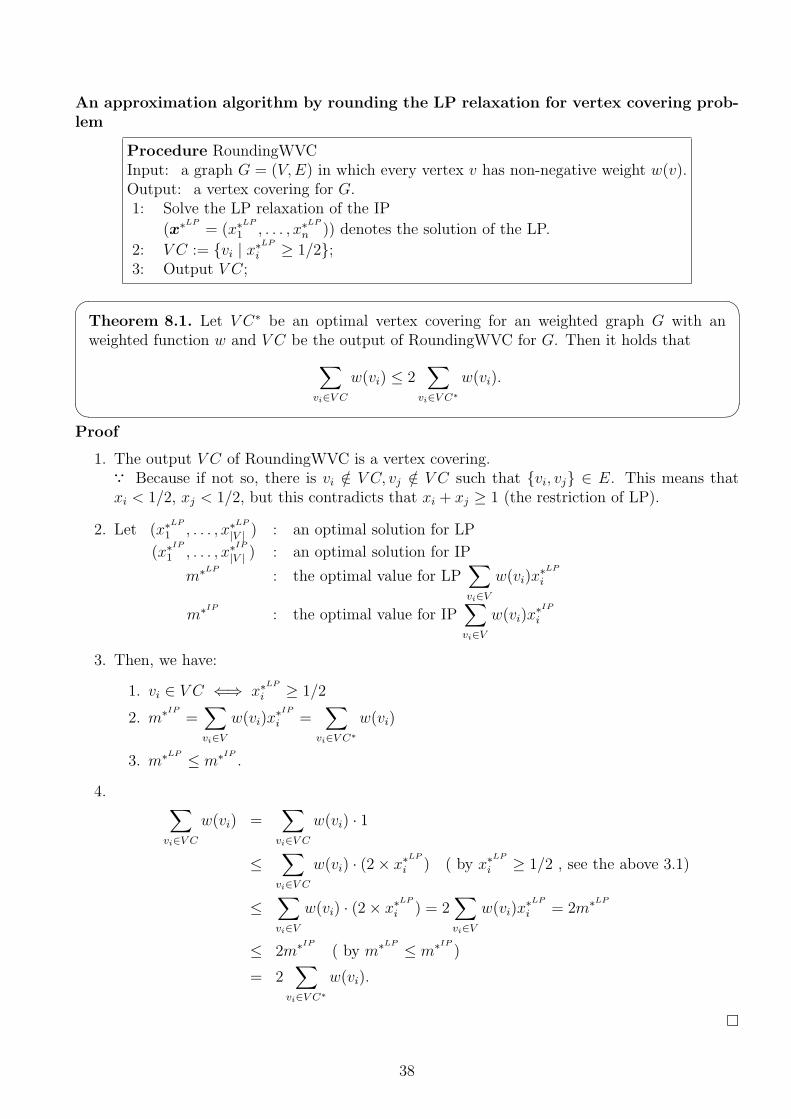
An approximation algorithm by rounding the LP relaxation for vertex covering prob-lem
Procedure RoundingWVCInput: a graph G = (V,E) in which every vertex v has non-negative weight w(v).Output: a vertex covering for G.1: Solve the LP relaxation of the IP
(x∗LP= (x∗LP
1 , . . . , x∗LP
n )) denotes the solution of the LP.
2: V C := {vi | x∗LP
i ≥ 1/2};3: Output V C;
� �Theorem 8.1. Let V C∗ be an optimal vertex covering for an weighted graph G with anweighted function w and V C be the output of RoundingWVC for G. Then it holds that∑
vi∈V C
w(vi) ≤ 2∑
vi∈V C∗
w(vi).
� �Proof
1. The output V C of RoundingWVC is a vertex covering.∵ Because if not so, there is vi /∈ V C, vj /∈ V C such that {vi, vj} ∈ E. This means thatxi < 1/2, xj < 1/2, but this contradicts that xi + xj ≥ 1 (the restriction of LP).
2. Let (x∗LP
1 , . . . , x∗LP
|V | ) : an optimal solution for LP
(x∗IP1 , . . . , x∗IP
|V | ) : an optimal solution for IP
m∗LP: the optimal value for LP
∑vi∈V
w(vi)x∗LP
i
m∗IP : the optimal value for IP∑vi∈V
w(vi)x∗IPi
3. Then, we have:
1. vi ∈ V C ⇐⇒ x∗LP
i ≥ 1/2
2. m∗IP =∑vi∈V
w(vi)x∗IPi =
∑vi∈V C∗
w(vi)
3. m∗LP ≤ m∗IP .
4. ∑vi∈V C
w(vi) =∑
vi∈V C
w(vi) · 1
≤∑
vi∈V C
w(vi) · (2× x∗LP
i ) ( by x∗LP
i ≥ 1/2 , see the above 3.1)
≤∑vi∈V
w(vi) · (2× x∗LP
i ) = 2∑vi∈V
w(vi)x∗LP
i = 2m∗LP
≤ 2m∗IP ( by m∗LP ≤ m∗IP )
= 2∑
vi∈V C∗
w(vi).
□
38

9 Primal-Dual Method
9.1 Basic knowledge of Primal Dual method� �Definition 9.1. (Canonical form of duality)Let
minimize z = ctxsubject to Ax ≥ b
x ≥ 0(P )
be a linear programming. The following linear programming is called dual problem of (P ):
maximize w = btysubject to Aty ≤ c
y ≥ 0.(D)
For the dual problem (D), (P ) is called by primal problem.� �� �Theorem 9.1. (Weak duality theorem)Let x be a feasible solution of (P ) and y be a feasible solution of (D). Then
w = bty ≤ ctx = z.� �
39

9.2 Basic idea of primal-dual method
• Although LP can be solved relatively easily, it takes a time in its own way.
• Clearly solving a linear programming is finding an optimal solution or computing the optimalvalue.
• Optimal solution is the best solution in the feasible solutions. So, finding an optimal solutioncosts more than finding a feasible solution.
Solving LP = Comp. OPT-SOL = Finding BEST ≥ Finding BETTER = Comp. FEA-SOL
• In the primal-dual metohd, we try to find a feasible solution of the dual programming insteadof finding an optimal solution. By this way, we can save the computational cost.
Combinatrial Problem
Primal LP Problem
Algorithm solving Primal LP Problem Algorithm finding a feasible
solution of Dual LP Problem +Algorithm finding a solution of Combinatrial Problem
duality
Rounding
Approximation Algorithm
Integer Programming
relaxation
Dual LP Problem
Approximation Algorithm
Figure 40: Outline of primal-dual method.
40

• From the point of view of approximation algorithms, (in the case of minimization problem)the point is that the value of a feasible solution can be considered as a lower bound for thecombinatorial problem (See Fig.41).
The value can be computed easily
A feasible solution of the Dual LP problem
Optimal solution of the Primal LP problem
Optimal solution of the integer programming
Lower bound of the optimal value
Figure 41: The point of primal-dual method.
41

9.3 An example: (weighted) vertex cover problem
• The linear relaxation of the integer programming for vertex cover problem can be representedby:
minimize w(vi)xi
subject to xi + xj ≥ 1 ∀{vi, vj} ∈ Exi ≤ 1 ∀vi ∈ V.
(LP )
• The dual linear programming of (LP ) can be represented by:
maximize∑
{vi,vj}∈E
yij
subject to∑
{vi,vj}∈E
yij ≤ w(vi) ∀vi ∈ V
yij ≥ 0 ∀{vi, vj} ∈ E
(DLP )
Note that we identify yij as yji.
• For instance, for the graph on the left side in Fig.42, from Ax ≥ b⇔ Aty ≤ c, we have:
1 2 2 2 2x1 x2 x3 x4 x5
y1,2 1 1 ≥ 1y2,3 1 1 ≥ 1y3,4 1 1 ≥ 1y4,5 1 1 ≥ 1y5,1 1 1 ≥ 1
⇔
1 1 1 1 1y1,2 y2,3 y3,4 y4,5 y5,1
x1 1 1 ≤ 1x2 1 1 ≤ 2x3 1 1 ≤ 2x4 1 1 ≤ 2x5 1 1 ≤ 2
• And from w = bty and y ≥ 0, (DLP ) can be represented by
maximize y1,2 + y2,3 + y3,4 + y4,5 + y5,1subject to y5,1 + y1,2 ≤ 1 (= w(v1))
y1,2 + y2,3 ≤ 2 (= w(v2))y2,3 + y3,4 ≤ 2 (= w(v3))y3,4 + y4,5 ≤ 2 (= w(v4))y4,5 + y5,1 ≤ 2 (= w(v5))yij ≥ 0 ∀{vi, vj} ∈ E
.
v1
v5
v4 v3
v2
1
2
2
2
2
v1
v5
v4 v3
v2
1
2
2
2
2
v1
v5
v4 v3
v2
1
2
2
2
2
v1
v5
v4 v3
v2
1
2
2
2
22 2 2 2 2
0
(0,2,0,0,0)(y12,y23,y34,y45,y51) (0,2,0,2,0) (0,2,0,2,0)
Figure 42: Process of Primal-DualWVC.
42

9.4 An approximation algorithm with primal-dual method for WVCproblem
Primal-DualWVCInput: a graph G = (V,E) in which every vertex v has non-negative weight w(v);Output: a vertex covering for G;
1 V C := ∅;2 for {vi, vj} ∈ E do3 yij := 0
4 while V C is not a vertex cover set do5 Pick an uncovered edge {vi, vj} ∈ E;
6 Increase yij up to∑
vk∈N(vi)
yik = w(vi) or∑
vk∈N(vj)
ykj = w(vj) ;
7 if∑
vk∈N(vi)
yik = w(vi) then
8 V C := V C ∪ {vi}9 else
10 V C := V C ∪ {vj}
11 return V C;� �Exercise 9.1. Is it true that Primal-DualWVC always outputs a minimal vertex covering?Prove it if so, disprove it if not so.� �
43

� �Theorem 9.2. Let G be a graph, V C∗ be an optimal vertex covering of G, V C be the outputof Primal-DualWVC for G. Then∑
vi∈V C
w(vi) ≤ 2∑
vi∈V C∗
w(vi).
� �Proof
1. From the construction, V C is a vertex covering.
2. Let m∗LP: the optimal value for LP
∑vi∈V
w(vi)x∗LP
i
m∗IP : the optimal value for IP∑vi∈V
w(vi)x∗IPi
3. For any feasible solution {yij | {vi, vj} ∈ E} of DLP , by weak duality theorem, we have∑{vi,vj}∈E
yij︸ ︷︷ ︸feasible sol. of DLP
≤ m∗LP︸ ︷︷ ︸opt. sol. of PLP
︸ ︷︷ ︸weak duality theorem
≤ m∗IP︸ ︷︷ ︸sol. of original problem
(6)
4.
∑vi∈V C
w(vi) =∑
vi∈V C
∑vj∈N(vi)
yij
by∑
vj∈N(vi)
yij = w(vi)
≤
∑vi∈V
∑vj∈N(vi)
yij
= 2∑
{vi,vj}∈E
yij
≤ 2m∗IP ( by Eq.(6))
□
44

9.5 Observation from the point of view of maximal solution
We consider PrimalDualWVC from the point of view of maximal solution.� �Definition 9.2. A feasible solution y of (DLP ) is maximal if there is no feasible solution yof (DLP ) such that
1. For each {vi, vj} ∈ E, yij ≥ yij, and,
2.∑
{vi,vj}∈E
yij >∑
{vi,vj}∈E
yij (Note that > not ≥).
� �MaximalPrimal-DualWVCInput: a graph G = (V,E) in which every vertex v has non-negative weight w(v).;Output: a vertex covering for G;
1 Find a maximal solution y of (DLP );
2 V C :=
vi
∣∣∣∣∣ ∑vj∈N(vi)
yij = w(vi)
;
3 return V C;
� �Theorem 9.3. Let G be a graph, V C∗ be an optimal vertex covering of G, V C be the outputof MaximalPrimal-DualWVC with G. Then,∑
vi∈V C
w(vi) ≤ 2∑
vi∈V C∗
w(vi).
� �Proof
1. V C is a vertex covering.
2. As in the case of Primal-DualWV,
∑vi∈V C
w(vi) =∑
vi∈V C
∑vj∈N(vi)
yij
by∑
vj∈N(vi)
yij = w(vi)
≤
∑vi∈V
∑vj∈N(vi)
yij
= 2∑
{vi,vj}∈E
yij
≤ 2m∗IP
□� �Exercise 9.2. Show that MaximalPrimal-DualWVC outputs a vertex covering.� �� �Exercise 9.3. Show that the approximation ratio of SimpleVC is 2, by using Theorem 9.3.� �
45

10 Fixed Parameter Tractability (FPT)
� �Definition 10.1. A problem P is Fixed Parameter Tractable (FPT) if for a parameterk, there are a constant which is not dependent on k and a function f(k) (not necessarilypolynomial on k), P can be solved in O(f(k)nc) time.� �• We call such an algorithm (realizing that complexity) FPT algorithm. We denote the setof FPT problems by FPT .
• The brute force approach (i.e. checking for all subset U ⊆ V of size k) costs O(nk), so theapproach is not FPT algorithm.
10.1 Fixed Parametrized Algorithm based on Search Tree� �Theorem 10.1. Let k be a fixed integer. For given a graph G = (V,E), it can be checked inO(2k|V (G)|) time whether there is a vertex covering of size k for G.� �
Proof
1. The following algorithm checks the problem in O(2k|V (G)|) time. (It is easy to modify thealgorithm to find a vertex covering of size at most k.)
FPTVC(G,k)
Input: A graph G = (V,E), positive integer k;
Output:
{Report ”YES” if there exists a veretex covering of size at most kReport nothing otherwise
1 if G has no edge then exit(YES) ; // failure → stop
2 if k = 0 then return; // failure → return
3 Chose an edge {u, v} in G;4 Construct the graph G− {u} by removing u and its incedent edges from G;5 FPTVC(G− {u},k − 1);6 Construct the graph G− {v} by removing v and its incedent edges from G;7 FPTVC(G− {v},k − 1);
2. FPTVC reports ”YES” iff there is a vertex covering of size at most k for G. The reason isas follows:
3. Let {u, v} be the edge chosen at step 3. Then either u ∈ U or v ∈ U holds.
4. So, ”G− {u} has a vertex covering of size at most k − 1 or ”G− {v} has a vertex coveringof size at most k − 1. At least one of the above two holds.
5. FPTVC repeats the process recursively, FPTVC finally outputs ”YES” if there exists (SeeFig.43).
6. The tree in Fig.43 is called by Serach Tree. Note that the size of search tree is only dependon k.
□
46

k=3
Figure 43: An example of search tree of FPTVC
47
10.2 Shrinking for search trees
• In the previous approach, for each selected edge {u, v}, we consider the two cases: u ∈ V Cand v ∈ V C.
• As opposed to the previous approach, here we choose a vertex, say v, then consider the twocases: v ∈ V C and v ̸∈ V C. By this approach, we can reduce the size of serach trees.
• To describe the new approach, it is enough to show that for each vertex v (in the search tree)what the children of v is. So we show it.
• Note that a vertex in the search tree corresponds to a subgraph of the input graph.
• Suppose that we are checking for the current graph G at a step. Without loss of generality,we can assume that G has a vertex of degree at least 3, because if not so G consists of pathsand/or cycles, so we can check quite easily.
• Let v be a vertex of degree at least 3 in G, w1, . . . , wp be the neighbors of v. The children ofthe vertex corresponding to G can be determined from v and w1, . . . , wp.
• The vertex corresponding to G has the following two children:
– The vertex corresponding to G− {v} (this is the case v ∈ V C),
– The vertex corresponding to G− {w1, . . . , wp} (this is the case v ̸∈ V C).
∵ In the case v ̸∈ V C, to cover the edges {v, w1} . . . , {v, wp}, the vertices {w1, . . . , wp}should be contained in V C (See Fig.45).
• – For the child G− {v}, we check whether G− {v} has a vertex covering of size at mostk − 1 or not.
– For the child G−{w1, . . . , wp}, we check whether G−{w1, . . . , wp} has a vertex coveringof size at most k − p or not.
– If p is large, the sub-search tree rooted by G−{w1, . . . , wp} should have small size. Notethat the point is the fact p ≥ 3.
• Let ak denote the size of serach tree for checking whether there is a vertex covering of sizeat most k for a graph. (Note that the size is not depend on the graph.)
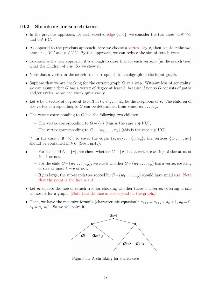
• Then, we have the recursive formula (characteristic equation): ak+3 = ak+2 + ak + 1, a0 = 0,a1 = a2 = 1. So we will solve it.
ak+3
ak ≧ ak+3-p
ak+2 = ak+3-1
Figure 44: A shrinking for search tree
48

• To solve it, let us try to set ak = ck. So solve ck+3 = ck+2 + ck (i.e. solving c3 = c2 + 1).Then we have c ≈ 51/4 (c < 51/4).
• Finally, we can have ak ≤ 5k4 − 1 for (k ≥ 2). (This can be shown easily by induction). So
we have the following theorem.
wp
w2
w1
···
v0
wp ∈ V C?
w2 ∈ V C?
w1 ∈ V C?
···
v0
wp ∈ V C
w2 ∈ V C
w1 ∈ V C
···
v0
The case of v0 ∈ V C
wi might be in VC or not.The case of v0 6∈ V C
w1, . . . , wp should be in VC.
Maximal degree< 3.
Degree of the vertex> (3 − 1).
Degree of the vertex> (3 − 1).
k = 3.
2
Figure 45: Shrinking for search trees
� �Theorem 10.2. There is an FTP algorithm of O(5k/4|V (G)|) running time for the vertexcover problem.� �
Proof
• Note that any induced graph G′ of G can be constructed in linear time.
• Because this can be done by keeping only the vertices by which G′ is induced.
• Note that the size of search tree is at most 5k/4, and the cost for each vertex (in the serachtree) is at most O(n).
□
49

10.3 Kernel reduction
In this subsection, we demonstrate a technique, so-called Kernel reduction.
FPTVC(G,k)
Input: A graph G = (V,E), positive integer k;
Output:
{Report ”YES” if there exists a veretex covering of size at most kReport nothing otherwise
1 Let S = {u1, . . . , up} be the set of vertices of degree more than k;2 if p > k then exit; // There is no small VC
3 k′ := k − p;4 Remove S and the incident edges with S and isolated vertices from G;5 // Denote the resulting graph by G′
6 if |V (G′)| > k′(k + 1) then exit; // There is no small VC
7 if G′ has no vertex covering of size at most k′ then // There is no small VC
8 exit9 else
10 Output the union of vertex covering of G′ and S.
• Any vertex covering of size at msot k for G should contain the set of vertices of degree morethan k (i.e., S ⊆ V C).
– Because if not so (i.e., there is a vertex v ̸∈ V C of degree more than k), then N(v)should be contained in V C, but we have contradiction k < |N(v)| ≤ |V C|.
• So G′ should be covered by a vertex covering of size at most k′ = k − p.
• The point is that G′ is the kernel part of G obtained from G by removing the nonessentialpart, and as we will see below, the size of kernel part G′ is bounded by a function of k(independent of n).
• If |V (G′)| > k′(k + 1), then there is no vertex covering of size at most k′ (See step 5).
– Let V C ′ be a vertex covering of size at most k′ for G′. Since
∗ each vertex in V (G′) \ V C ′ is adjacent to a vertex in V C ′, and
∗ every vertex in G′ (thus, V C ′) has degree at most k, and
∗ G′ has no isolated vertex.
So |V (G′) \ V C ′| is at most k′k.
– From V (G′) = V C ′ ∪ V (G′) \ V C ′, we have |V (G′)| ≤ |V C ′|+ |V (G′) \ V C ′| ≤ k′ + k′k.
• The check in step 1 can be done O(k|V (G)|) time. From Theorem 10.2, the check for step 6can be done O(5k/4 · k2) time (Note that k′ ≤ k). So we have the following theorem.
� �Theorem 10.3. The running tiime of KernelReductionFPTVC(G,k) is O(5k/4 ·k2+k|V (G)|).� �
50

11 Nonconstructive methods
11.1 Probabilistic Method
• We consider here methods for proving the existence of a solution.
• For example, consider the following question:
Problem Students in a class had a math. exam and the average score is 50 points. Is therea student who scores at least 50 points?
• How to prove the existence? The simple and natural way is to find such a student. This way(finding such a student) is sufficient to answer the question. Is this “finding” necessary toanswer the question?
• Now we have a question: Can we show the existence without finding a student?
• In this lecture, the method by finding a student is called constructive method, and themethod without finding is called nonconstructive method.
• In this section we demonstrate a technique so-called ”Probabilistic Method”, which is oftenused to prove ”existence”.
• By using Probabilistic Method, we can answer the question: Let n be the number of studentsand X be the average score. If there is no student who scores at least 50 points, that is, if allstudent score less than 50 points, then X should be less than 50, this contradicts X ≥ 50.� �
Theorem 11.1. A graph G = (V,E) has an independent set of size at least |V |/(2δ), whereδ = δ(G) denotes the average degree of G.� �
Proof
1. Let S ⊆ V be a random subset of V with the probability Pr[v ∈ S] = p. Let X = |S| andY be the number of edges in G[S].
2. For each edge {u, v} = e ∈ E, random variable Ye is defined as the following:
Ye =
{1 u ∈ S and v ∈ S0 otherwise.
Thus, Y =∑
e∈E Ye.
3. ClearlyE[Y{u,v}] = Pr[(u ∈ S) and (v ∈ S)] = p2.
4. From the linearity of expectation and |E| = |V |δ/2, we have
E[Y ] = E
[∑e∈E
Ye
]=∑e∈E
E[Ye] =|V |δ2
p2.
5. From E[X] = |V |p (and the linearity of expectation again), we have
E[X − Y ] = |V |p− |V |δ2
p2. (7)
51

6. The equation 7 reaches the maximaum when p = 1/δ, and the maximaum value is
E[X − Y ] =|V |2δ
.
7. We can have an independent set from S by removing vertices of degree at least 1. The expec-tation of the size of the independent set is at least |V |
2δ. So there there exists an independent
set of size at least |V |/(2δ).
□� �Theorem 11.2. A graph G = (V,E) has an independent set of size at least
∑v∈V
1
degG(v) + 1.
� �Proof (nonconstructive)
1. Let < be a uniformly chosen total ordering of V . Define I = {v ∈ V | {v, w} ∈ E ⇒ v < w}.Note that I is an independent set of G.
2. Let
Xv =
{1 v ∈ I0 otherwise.
Thus, X =∑
v∈V Xv = |I|.
3. For each vertex v,
E[Xv] = Pr[v ∈ I] =1
degG(v) + 1. (8)
4. Hence the expectation of X is
E[X] =∑v∈V
1
degG(v) + 1
Therefore, there must exist an independent set I such that |I| ≥∑v∈V
1
degG(v) + 1.
□� �Exercise 11.1. Prove that I is an independent set of G.� �� �Exercise 11.2. Prove the equation (8).� �
Proof (constructive)
1. For a graph G and a vertex v in G of minimum degree, the following holds:∑u∈{v}∪NG(v)
1
dG(u) + 1≤ 1. (9)
52

2. Furthermore the following holds:∑u∈V
1
dG(u) + 1≤ 1 +
∑u∈V−
({v}∪NG(v)
) 1
dGv(u) + 1
Because, ∑u∈V
1
dG(u) + 1=
∑u∈({v}∪NG(v)
) 1
dG(u) + 1+
∑u∈V−
({v}∪NG(v)
) 1
dG(u) + 1
≤ 1 +∑
u∈V−({v}∪NG(v)
) 1
dGv(u) + 1(9) より (10)
Figure 46: Inequation (10)
3. The following algorithm outputs an independent set of size at least∑v∈V
1
degG(v) + 1.
GreedyMIS
Input: A graph G = (V,E);Output: an independent set
1 S := ∅;2 while E(G) ̸= ∅ do3 Chose a vertex v ∈ V (G) of minimum degree;4 S := S ∪ {v};5 G := G−
{{v} ∪NG(v)
};
6 Output S;
53

4. Because, from the equation (10),∑u∈V
1
dG(u) + 1≤ 1 +
∑u∈V−
({v}∪NG(v)
) 1
dG(u) + 1
≤ 2 +∑
u∈V−({v}∪NG(v)
) 1
dG(u) + 1(G, v in the 2nd loop)
...
≤ |S| − 1 +∑
u∈V−({v}∪NG(v)
) 1
dG(u) + 1
(G is the graph just before the empty graph)
≤ |S|
Hence, the theorem holds.
□� �Exercise 11.3. Prove the equation (9).� �
54

11.1.1 Max cut� �Theorem 11.3. A graph G = (V,E) has a cut (V1, V2) of size at least |E|/2.� �
Proof (By Probabilistic Method, nonconstructive)
1. Color each vertex v ∈ V with red or blue with a probability of 1/2. Consider the set ofvertices colored with red and blue as V1 and V2 respectively.
2. Define random variable Xe for each e ∈ E as follows:
Xe =
{1 the endpoints of e have different colors0 otherwise.
3. Let X be the size of the cut (V1, V2). So X =∑
e∈E Xe.
4. The probability of X{u,v} = 1 is 1/2. So E[Xe] = 1/2.
5. Thus,
E[X] = E
[∑e∈E
Xe
]=∑e∈E
E[Xe] = |E|/2
6. Therefore there is a cut of size at least |E|/2.
□
Proof (By Local Search, constructive)
1. What is Local Search?
1
4311
3 2 2 4
23 3
65 3
4
2
12
3
maximum
maximal
maximal maximal
12
3
maximum
maximal
maximal
12
3
maximum
maximal
v
neighbor of solution v
Image (Solution Space)Image (Hill Climbing)
Figure 47: Image of Local Search.
2. The solution space of max-cut problem consists of S = {(V1, V2) | V1 ⊆ V, V2 = V − V1}.
55

3. The neighbors of a cut C = (V1, V2) ∈ S is defined by the set of cuts obtained from C byapplying one of the following two operations:
1. a vertex in V1 is moved into V2 or
2. a vertex in V2 is moved into V1.
4. The following algorithm output a cut of size at least |E|/2.
Procedure MaxCutLocalSearchInput: a graph G = (V,E)Output: a cut of size at least |E|/21: C := a cut C;2: while there is a neighbor C ′ of C such that |C ′| > |C| do3: C := C ′;4: od5: output C;
5. Fig. 48 illustrates an example of local search for max-cut problem. In this example, C0 =({v6}, {v1, v2, v3, v4, v5})is chosen as initial solution. The value of C0 is 4. From the neighborsof C0, C1 = ({v3, v6}, {v1, v2, v4, v5}) is chosen. The value of C0 is 6.
Figure 48: An example of local search.
6. As shown in Fig. 49, C1 is a local optimal solution, since there is no better neighbor of C1
than C1.
v1
v2
v3
v6
v5
v4
v1
v2
v3
v6
v5
v4
v1
v2
v3
v6
v5
v4
v1
v2
v3
v6
v5
v4
v1
v2
v3
v6
v5
v4
v1
v2
v3
v6
v5
v4
V1={v3,v6}
V2={v1,v2,v4,v5}
局所解(6本)
v1
v2
v3
v6
v5
v4
V1={v1,v3,v6}
V2={v2,v4,v5}
V1={v2,v3,v6}
V2={v1,v4,v5}
V1={v3,v4,v6}
V2={v1,v2,v5}
V1={v3,v5,v6}
V2={v1,v2,v4}
V1={v6}
V2={v1,v2,v3,v4,v5}
V1={v3}
V2={v1,v2,v4,v5,v6}
Figure 49: An example of local solution.
56

7. Let C be an output of MaxCutLocalSearch, and m1 and m2 be the numbers of edges in G[V1]and G[V2] respectively. Then
|E| = m1 +m2 + |C|. (11)
8. Letm1(vk) = {v | v ∈ V1 and {v, vk} ∈ E}m2(vk) = {v | v ∈ V2 and {v, vk} ∈ E}.
9. Since C is a local optimal solution,
∀vk ∈ V1, |m1(vk)| − |m2(vk)| ≤ 0
∀vk ∈ V2, |m2(vk)| − |m1(vk)| ≤ 0
∵ If a vertex vk ∈ V1 moves into V2 then the size of the cut (V1 − {vk}, V2 ∪ {vk}) in-creases |m1(vk)| and decreases |m2(vk)|. Since the total does not increase, we have |m1(vk)|−|m2(vk)| ≤ 0 (the case vk ∈ V2 can be shown similarly).
Figure 50: Inequation
10. By taking sum over all the vertices in V1,∑vk∈V1
(|m1(vk)| − |m2(vk)|) = 2m1 − |C| ≤ 0 (12)
∵ For an edge {v, vk}, the edge is counted twice if v ∈ V1, and is counted only once if v ̸∈ V1.
11. Similarly by taking sum over all the vertices in V2, we have∑vk∈V2
(|m2(vk)| − |m1(vk)|) = 2m2 − |C| ≤ 0. (13)
12. By taking the sum eq. (12) and eq. (13),
2m1 + 2m2 − 2|C| ≤ 0⇒ m1 +m2 ≤ |C|. (14)
13. By substituting eq. (14) into eq. (11),
|E| = m1 +m2 + |C| ≤ 2|C|
Therefore we have |C| ≥ |E|/2.
□
57

11.2 Graph minor and Wagner’s conjecture
11.2.1 Graph minor� �Definition 11.1. (minor)A graph H is minor of a graph G, denoted by H ≤m G if H can be obtained from G byapplying repeatedly the following operations:
1. contraction of an edge, or
2. deletion of an isolated vertex or an edge.� �Fig. 51 illustrates an example of minor.
削除宿約
削除
宿約
Figure 51: An example of minor.
� �Definition 11.2. ( minor-closed-family)A class F of graphs is called minor-closed-family if
H ∈ F , G ≤m H ⇒ G ∈ F .� �� �Definition 11.3. (obstruction set)A class O of graphs is called obstruction set of F if
G ∈ F ⇐⇒ ∀H ∈ O, H ̸≤m G.� �For example, the obstruction set of planar graphs is {K5, K3,3}. 2� �Theorem 11.4. Let H be a fixed graph and G be an input graph. Then the decision problemwhether H ≤m G or not can be solved in O(|V (G)|3) time.� �
11.2.2 Wagner’s conjecture
Wagner’sconjecture was answered affirmatively by Robertson and Seymour in the second half of1980’.� �Theorem 11.5. For any minor-closed-family, its obstruction set is finite.� �
Combining Theorem 11.4 and Wagner’s conjecture, we have the following theorem.
2This is the version of not ”homeomorphic” but ”minor” of Kuratowski theorem.
58

� �Theorem 11.6. Let F be a minor-closed-family. For a graph G, there exists an algorithmsolving the problem whether or not G ∈ F in O(|V (G)|3) time.� �
Proof Sketch of the proof.
1. Let {H1, · · · , HnF} be the obstruction set of F . The algorithm just checks ”Hi ≤m G” foreach Hi (1 ≤ i ≤ nF).
2. 1. Since nF is independent of G, nF can be seen as a constant.3
2. The check ”Hi ≤m G” can be done in O(n3) time.
Thus, the running time of the algorithm is O(n3).
□
The problem is how to find the obstruction set. Unfortunately it is undecidable to determinewhether or not the obstruction set is empty.
So we do not know concretely the obstruction set, but we know it should be finite.
3The hidden constant is quite large.
59

12 Nemhauser-Trotter Theorem
• Recall that the linear relaxation of the integer programming for vertex cover problem can berepresented by:
minimize w(vi)xi
subject to xi + xj ≥ 1 ∀{vi, vj} ∈ Exi ≤ 1 ∀vi ∈ V.
(LP )
• We frequently use xvi instead of xi, specially xv for v ∈ V .
• It is known that (LP) has always an optimal solution with the property that the variablestake one of three possible values {0, 1
2, 1}. We will use this fact, but not prove here.
• Let Vℓ (ℓ ∈ {0, 12 , 1}) denote the set of vertices whose fractional values are ℓ.
Theorem 12.1. (Nemhauser and Trotter)There exists an optimal solution OPT with the following properties:
(a) OPT is a subset of (V1 ∪ V 12),
(b) OPT includes all of V1.
Remarks. In the proof, we use often arguments by contradiction. There are mainly two types:
• contradiction to optimality of the LP solution,
• contradiction to the fact that OPT covers all edges.
Proof We first show that (a)⇒ (b).
• Suppose to the contrary that OPT does not include v ∈ V1.
• case[(N(v) ∩ V0) = ∅]
– subcase[w(v) = 0]We can add v to OPT without increasing the weight.
– subcase[w(v) > 0]The fractional value xv can be reduced. ∵ In this case, we do not need to consider thecase “xu(= 0)+xv(= 1) ≥ 1” because of (N(v)∩V0) = ∅ (Also not need for “xu(= 1)+xv(= 1) ≥ 1”). That is, we need to consider only the case “xu(= 1/2)+xv(= 1/2) ≥ 1”.So we can have a better LP solution (See Fig. 52 (a)).
• case[u ∈ (N(v) ∩ V0) ̸= ∅]For u ∈ N(v) ∩ V0, {u, v} is not covered in OPT . (See Fig. 52 (b)).
v
V0 V1 V1/2
v
V0 V1 V1/2
v
V0 V1 V1/2
OPTOPT OPT
(a) (b)u
Figure 52: (a)⇒ (b)
60

We now prove (a).
• Suppose to the contrary that OPT ∩ V0 ̸= ∅.
• Let BI denote the set (OPT ∩ V0) (So BI ̸= ∅), and LO denote the set V1\OPT .
• The vertices in BI can have only edges going to vertices in V1, otherwise the edges do notsatisfy the LP constraint (See Fig. 53 (a)).
• The edges going to LO can be classified into two types:
– edges exactly one endpoint is covered by OPT ,
– edges both endpoints are covered by OPT .
• There is no edge between u ∈ (V0\OPT ) and v ∈ LO, because OPT does not cover such anedge (See Fig. 53 (a)).
• – case[w(BI) ≥ w(LO)]We can replace BI by LO in OPT without increasing the weight of OPT , and the newOPT satisfies (a). (See Fig. 53 (b)).
– case[w(BI) < w(LO)]For each vertices in BI and LO, and 0 < ϵ ≤ 1
2, modify
∗ x′u := xu + ϵ for u ∈ BI ,
∗ x′v := xv − ϵ for v ∈ LO, and
∗ x′w := xw for w ∈ BI ∪ LO.
Thus, we have a new solution (x′v1, . . . , x′
vn) of the LP problem. The cost of new solutionis the cost of old solution plus ϵ · (w(BI)− w(LO)). Thus, as w(BI) < w(LO), the newsolution is better than the old solution, a contradiction (See Fig. 53 (b)).
□V0 V1 V1/2
OPT
(a)
BI
LO
0+1/2<1
0+0<1
V0 V1 V1/2
OPT
(b)
BI
LO
+ε
-ε
exchange
Figure 53: Figures in the proof of (a)
• The theorem implicitly show that the approximation ratio of RoundingWVC (in Section 8)is two. This is because:
• Denote the optimal solution in Theorem 12.1 by OPT . We also denote OPT ∩ V1/2 OPT1/2.Recall that V1∪V1/2 ⊇ OPT ⊃ V1. Note that the output OUT of RoundingWVC is V1∪V1/2.
• Since 0 · w(V0) +12· w(V1/2) + 1 · w(V1) is a lower bound for the optimal value, we have
w(V1) +12w(V1/2) ≤ w(OPT ) = w(V1) + w(OPT1/2).
• Hence, 12w(V1/2) ≤ w(OPT1/2), i.e., w(V1/2) ≤ 2w(OPT1/2) holds. So, we have
w(OUT )
w(OPT )=
w(V1) + w(V1/2)
w(V1) + w(OPT1/2)≤
w(V1) + 2w(OPT1/2)
w(V1) + w(OPT1/2)≤ 1 +
w(OPT1/2)
w(V1) + w(OPT1/2)≤ 2.
61
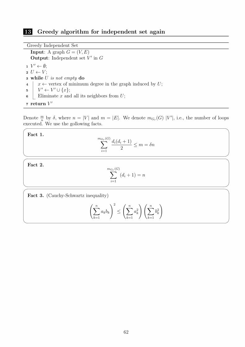
13 Greedy algorithm for independent set again
Greedy Independent Set
Input: A graph G = (V,E)Output: Independent set V ′ in G
1 V ′ ← ∅;2 U ← V ;3 while U is not empty do4 x← vertex of minimum degree in the graph induced by U ;5 V ′ ← V ′ ∪ {x};6 Eliminate x and all its neighbors from U ;
7 return V ′
Denote mn
by δ, where n = |V | and m = |E|. We denote mGr(G) |V ′|, i.e., the number of loopsexecuted. We use the gollowing facts.� �Fact 1.
mGr (G)∑i=1
di(di + 1)
2≤ m = δn
� �� �Fact 2.
mGr (G)∑i=1
(di + 1) = n
� �� �Fact 3. (Cauchy-Schwartz inequality)(
n∑k=1
akbk
)2
≤
(n∑
k=1
a2k
)(n∑
k=1
b2k
)� �
62

� �Lemma 13.1.
n(2δ + 1) ≥mGr (G)∑
i=1
(di + 1)2 ≥ n2
mGr(G)i.e., mGr(G) ≥ n
2δ + 1=
n
δ̄ + 1.
� �Proof
• By Fact 1 and Fact 2,
mGr(G)∑i=1
di(di + 1)
2≤ δn
⇒mGr(G)∑
i=1
di(di + 1) ≤ 2δn
⇒mGr(G)∑
i=1
di(di + 1) +
mGr(G)∑i=1
(di + 1) ≤ 2δn+ n
⇒mGr (G)∑
i=1
(di + 1)2 ≤ n(2δ + 1)
• By Fact 3, mGr (G)∑i=1
(di + 1)
2
≤
mGr (G)∑i=1
(di + 1)2
mGr (G)∑i=1
12
≤ mGr(G) ·
mGr (G)∑i=1
(di + 1)2
• By Fact 2, the leftside
mGr (G)∑i=1
(di + 1)
2
is n2.
• So, we have thatn2
mGr(G)≤
mGr (G)∑i=1
(di + 1)2.
□
• Fix a maximum independent set V ∗ and let ki be the number of vertices in V ∗ that aredeleted in the i-th iteration of the while loop in the algorithm.
• Then, we have:mGr(G)∑
i=1
ki = |V ∗| = m∗(G)
63

� �Lemma 13.2.
mGr(G)∑i=1
((di + 1)2 + k2
i
)≤ n(2δ + 1) +m∗(G)
� �Proof From Figure 54, it is not difficult to verify the following::
mGr(G)∑i=1
di(di + 1) + ki(ki − 1)
2≤ δn
If we do not know ki, we have to consider the worst case..
64 4 1274
m*
m*
If we know ki, then we can ...
Figure 54: Why +ki(ki − 1)?
mGr(G)∑i=1
di(di + 1) + ki(ki − 1)
2≤ δn
⇒mGr(G)∑
i=1
di(di + 1) + ki(ki − 1) ≤ 2δn
⇒mGr(G)∑
i=1
di(di + 1) +
mGr(G)∑i=1
ki(ki − 1) ≤ 2δn
⇒mGr(G)∑
i=1
di(di + 1) +
mGr(G)∑i=1
(di + 1) +
mGr(G)∑i=1
ki(ki − 1) ≤ 2δn+ n
⇒mGr(G)∑
i=1
(di + 1)2 +
mGr(G)∑i=1
ki(ki − 1) +
mGr(G)∑i=1
ki ≤ 2δn+ n+m∗(G)
⇒mGr(G)∑
i=1
(di + 1)2 +
mGr(G)∑i=1
k2i ≤ n(2δ + 1) +m∗(G)
□
64

� �Theorem 13.3.
m∗(G)
mGr(G)≤ δ + 1 =
δ̄
2+ 1
� �Proof
• By Lemma 13.2,mGr(G)∑
i=1
((di + 1)2 + k2
i
)≤ n(2δ + 1) +m∗(G)
• By Fact 3 ,
m∗(G)2 =
mGr(G)∑i=1
(ki · 1)2 ≤mGr(G)∑
i=1
k2i ·
mGr(G)∑i=1
12 = mGr(G)
mGr(G)∑i=1
k2i
• By Lemma 13.1,
n(2δ + 1) +m∗(G) ≥mGr(G)∑
i=1
((di + 1)2 + k2
i
)≥ n2 +m∗(G)2
mGr(G)
• Thus,
mGr(G) ≥ m∗(G) · (n/m∗(G)) + (m∗(G)/n)
2δ + 1 + (m∗(G)/n)
• The inequality can be minimized by setting m∗(G) = n, by which we can have the theorem.Hence,
mGr(G) ≥ m∗(G) · 2
2δ + 2= m∗(G) · (δ + 1).
□
References
[1] G. Ausiello, P. Crescenzi, G. Gambosi, V. Kann, A. Marchetti-Spaccamela, M. Protasi “Com-plexity and Approximation Combinatorial optimization problems and their approximabilityproperties”, Springer Verlag, ISBN 3-540-65431-3.
[2] Christos H. Papadimitriou, Kenneth Steiglitz, “Combinatorial Optimization: Algorithms andComplexity”.
65