N92-15459

Theory and ObservationsModel Simulations of the

Period 1955-- 1985

I*

Panel Members

S. A. Isaksen, Chair

R. Eckman

A. LacisM. Ko -- /q& 5--2.5"7Jo

M. Prather _ _e q4qq (e,7

J. pyle -- ogg,(ot oblH. RodheF. Stordal _@ o_7 9b'7_-

R. Stolarski - t? C q q 4 _ &7

R. P. Turco _D. Wuebbles L}q 6_ 5" 0"?5"

z

7!-!!!_

®

ilB!i!Hmmm

=jzJ

https://ntrs.nasa.gov/search.jsp?R=19920006241 2018-07-06T00:33:12+00:00Z

Chapter 7

Theory and ObservationsModel Simulations of the Period 1955-1985

7.2

7.3

Contents

INTRODUCTION .......................................................... 503

ATMOSPHERIC SCENARIOS FOR 1955-1990 ................................. 503

7.1.1 Trace Gases .......................................................... 504

7.1.2 Solar Variability ....................................................... 5067.1.3 Nuclear Test Series .................................................... 507

7.1.4 Atmospheric Variations Not Modelled .................................. 508

THE

7.2.1

7.2.2

7.2.3

7.2.4

7.2.5

MODELS ............................................................. 508

Model Descriptions ................................................... 508Basic Chemical Uncertainties ........................................... 511

Uncertainties in Transport ............................................. 512

Comparison of Models With the Contempora D" Atmosphere .............. 513

Stratospheric Temperature Feedbacks ................................... 521

MODEL SIMULATIONS OF OZONE CHANGE ............................... 521

7.3.1 Calculated Total Global Variations ...................................... 522

7.3.2 Atmospheric Nuclear Tests ............................................ 5237.3.3 Column Ozone: Comparison With Observations ......................... 525

7.3.3.1 Theoretical Fingerprints for the Solar Cycle and Trace Gases ...... 525

7.3.3.2 Thirty Years of Dobson Data ................................... 5277.3.3.3 Global Data From Satellite, 1979-1987 ........................... 527

7.3.3.4 Subtracting the Solar Cycle From Dobson Data ................... 531

7.3.4 Profile Ozone: Comparison With Observations .......................... 532

7.3.4.1 Fingerprints of the Solar Cycle and Trace Gases .................. 5327.3.4.2 Trends in Vertical Structure, 1979-1985 .......................... 535

7.3.5 Tropospheric Ozone ................................................... 5367.3.5.1 Impact on Column Perturbations ............................... 5367.3.5.2 Uncertainties in the Estimates .................................. 537

7.3.6 Future Ozone Changes (1985-1990) ..................................... 5387.3.7 How Good Are the Models? ........................................... 539

7.4 CONCLUSIONS ........................................................... 539

501

PRECEDING PAGE BLA_'_K NOT F!LMED

°

THEORY AND OBSERVATIONS

7.0 INTRODUCTION

The main objective of the theoretical studies presented here is to apply models of strato-

spheric chemistry and transport in order to understand the processes that control stratospheric

ozone and that are responsible for the observed variations. The model calculations are intended

to simulate the observed behavior of atmospheric ozone over the past three decades (1955-1985),for which there exists a substantial record of both ground-based and (more recently) satellite

measurements. Through comparisons of the modeled history of atmospheric ozone with these

data, we hope to:

• Simulate the observed temporal and spatial variations of ozone.

• Focus on the specific patterns, or "fingerprints," of ozone change that, according to currentunderstanding, can be uniquely associated with a specific cause.

• Identify the roles of human activity, solar cycle variations, and other undetermined natural

variability in altering stratospheric ozone.

• Evaluate the reliability of models for stratospheric ozone and their ability to predict change.

The development of two-dimensional (2-D) models of stratospheric chemistry and transport

has led to considerable improvement in our ability to describe the stratosphere, to predict ozone

distributions, and to compare with observations of ozone and other trace compounds (see WMO,

1986). Two-dimensional calculations allow us to simulate both the latitudinal and seasonal

variations in the stratosphere, a task beyond the scope of the 1-D models traditionally used for

assessment. Results from the 2-D models may allow for identification of fingerprints in ozone:i.e., certain months and latitudes for which chlorofluorocarbon (CFC)-induced ozone effects are

most pronounced. We have chosen to base our present study on results from 2-D models. Wehave included for historical perspective some results from parallel 1-D models (from the same

research groups as for 2-D models), but find that 1-D models cannot be used to predict even the

globally averaged perturbations to ozone.

Although many features in these atmospheric simulations are common to all models,

significant differences exist. There are systematic discrepancies in all of the models with regardto the absolute concentrations of ozone at the stratopause and the source of odd nitrogen in the

lower tropical stratosphere. These stratospheric models represent the most recent versionsavailable from the research groups involved, and thus are not fully or, in some cases, partly

documented in the published literature. A detailed intercomparison of the 2-D models has not

yet been made, but is planned for 1988. For these reasons, we have incorporated a brief section

on comparison with observations and an extended discussion on uncertainties pertinent to the

model calculations in this study.

7.1 ATMOSPHERIC SCENARIOS FOR 1955-1990

The period of focus for this study was selected to be the last 30 years, because there is anextensive data base collected on total column ozone by the Dobson network for this period,

starting with the International Geophysical Year, 1957. Factors that could have influenced

atmospheric ozone during this period include slow increases in the concentration of biogenic/

anthropogenic trace gases such as carbon dioxide (CO2), methane (CH4), and nitrous oxide

5O3

_..._C)_ tcn_E_Ti(_Nr,l._vIi"AB ,. PRBCEDING PAGE BLANK NOT FILMED

THEORY AND OBSERVATIONS

(N20); a rapid rise in the concentration of stratospheric chlorine from the manmade gases CFCI3,

CF2CI2, carbon tetrachloride (CCl4), and methylchloroform (CH3CC13); injection of nitrogen

oxide (NO) by atmospheric nuclear tests; and variations in ultraviolet (UV) sunlight over the

ll-year solar cycle. These terms have been included in the model scenarios selected here. Other

geophysical factors that lead to noticeable changes include changes in tropospheric chemistryand climate, increases in brominated halocarbons, volcanos, heterogeneous chemistry in the

polar stratosphere, and changes in circulation associated with the quasi-biennial oscillation(QBO) and the E1 Nifio/Southern Oscillation (ENSO). The neglect of these latter terms isdiscussed with the uncertainties in the models. Table 7.1 indicates the combinations of factors

that are incorporated in the different calculations.

In addition to the primary period, 1955-1985, we believe it is important to extend the

calculations through 1991 in order to predict near-term global trends in ozone as we approach the

next maximum in the solar cycle. A realistic assessment of the predictions of ozone change is

needed since, according to current theory, increases in ozone caused by increasing solar

intensity could fully or partially cancel the calculated ozone decreases caused by the effect of

trace gases, as described below.

Table 7.1 Factors Included in Model Simulations

Case CFC's N20 _a: CH4 solar nuclear T _ CO 2

1 yes yes no no (some)

2 yes yes yes no (some)

3 yes yes yes yes (some)

Case 1 illustrates the effects of changes in trace gases only. In case 2, the effects of the solar

cycle are introduced through cyclic changes in the solar ultraviolet (UV) flux. In case 3, releases of

NO from atmospheric nuclear tests during 1958-1962 are included. Changes in stratospheric

temperature will be driven by changes in CO2 and 03; some of the models were able to includethis feedback, others were not (see model description below).

7.1.1 Trace Gases

Emissions and atmospheric concentrations of important trace gases, such as CO2, CH4, NaO,

and several chtorocarbons, are known to have increased substantially over 1955-1985. Scenarios

for the historical variations in these gases are based on observed increases in concentrations or onestimates of the emissions of these gases (Wuebbles et al., 1984), as outlined in Table 7.2. The

scenarios employed here represent one possible reconstruction of the recent composition of the

atmosphere. Nevertheless, the uncertainties in the trace gas composition of the atmosphere over

Table 7.2 Trace Gas Scenarios Adopted for 1950-1991

CO2 (ppm) 270 x (1.00141)" _s_} t <1958.0270 + 44.4 x (1.0192f _9_) t >1958.0

CH4 (ppm) 0.70 + 0.93 x (1.018y' _"_'_ t <1980.01.63 x (1.010y '-I°s°_ t >1980.0

N20 (ppb) 285 + 14.0 x (1.041y '-1"7_ all t

Concentrations refer to bulk tropospheric values; t is time in years. Based on fits supplied by D. Wuebbles (see Wuebbles et aI., 1984).

5O4

THEORY AND OBSERVATIONS

the last three decades are bounded by measurements, and alternate scenarios that are consistent

with observations would not produce significantly different results in these models.

Yearly release rates of chlorocarbons are given in Table 7.3 for each year between 1955 and

1985. Fluxes of chlorocarbons are assumed to be constant after 1985. Other trace gases, such as

CO and NO× ( = NO + NO2), which may have had important effects on tropospheric ozone, are

kept at a constant level, partly due to major uncertainties about their emissions over this time

period and partly due to the uncertainties connected to the treatment of tropospheric chemistry

in the present models. For example, aircraft emissions of NO× were not included; there areuncertainties in theoretical emission rates, in addition to uncertainties in how to model the

tropospheric NO× and ozone (03). Carbon monoxide (CO) increases are not considered,

although there are indications that Northern Hemispheric levels have been increasing slowly

(see Chapter 8). Halon (bromocarbon) scenarios were not included because the increase in

Table 7.3 Fluorocarbon Emission Fluxes (109g/yr) Used in Models for 1950-1991

Year CFCI3 CF2Cl2 CHCIF2 C2C13F3 CCl4 CH3CCI3(CFC-11) (CFC-12) (CFC-22) (CFC-113)

1955 21.5 46.9 0.6 0.0 91.0 3.4

1956 26.1 53.3 0.8 0.0 87.9 7.4

1957 31.3 60.5 1.1 0.0 84.8 16.4

1958 31.3 68.6 1.4 0.0 84.8 19.6

1959 31.3 77.9 1.9 0.0 84.8 23.3

1960 38.2 88.5 2.6 2.5 84.8 27.8

1961 47.3 100.5 3.5 3.0 84.8 33.0

1962 58.5 114.1 4.2 3.7 84.8 39.2

1963 72.4 129.5 5.1 4.4 88.7 46.6

1964 88.7 148.2 6.1 5.4 92.8 55.51965 100.8 167.6 7.3 6.5 97.0 65.9

1966 114.6 189.5 8.8 7.9 101.5 78.4

1967 130.2 214.3 10.6 9.6 106.1 93.2

1968 148.0 242.4 I2.7 11.6 111.0 110.8

1969 168.2 274.1 15.3 14.0 116.1 131.71970 191.2 300.5 18.3 17.0 121.4 156.6

1971 217.3 327.9 22.0 20.6 127.0 186.2

1972 247.0 357.9 26.5 24.9 132.9 221.3

1973 280.7 390.6 31.8 30.2 139.0 263.1

1974 323.5 443.5 38.3 36.6 145.3 312.8

1975 323.5 434.6 46.0 44.3 131.2 37 I. 9

1976 323.5 433.9 50.3 53.6 131.2 442.1

1977 325.5 418.0 55.0 65.0 131.2 454.51978 316.5 388.6 60.1 74.4 131.2 454.5

1979 307.8 388.6 65.7 85.1 131.2 454.5

1980 264.5 388.6 71.9 97.3 131.2 454.5

1981 264.5 412.2 71.9 97.3 131.2 454.5

1982 264.5 412.2 71.9 97.3 131.2 454.5

1983 264.5 412.2 71.9 97.3 131.2 454.5

1984 264.5 412.2 71.9 97.3 131.2 454.5

1985 264.5 412.2 71.9 97.3 131.2 454.5

505

THEORY AND OBSERVATIONS

stratospheric bromine from manmade halocarbons is expected to have had only a minor effect on

ozone through 1985. (A notable exception may be the polar ozone reductions, which are notaddressed in these calculations.)

7.1.2 Solar Variability

Variations in sunlight over the 11-year solar cycle are believed to manifest themselves as

cyclic changes in the solar flux on the order of 10 percent or less in the far ultraviolet, with verysmall changes, if any, in the visible region of the spectrum. The far UV--wavelengths less than

220 nm--is responsible for photolysis of 02 and, hence, primary production of ozone. (Destruc-

tion of ozone is driven, in general, by wavelengths longer than 240 nm.) The maximum in solarUV is associated with the maximum of the solar cycle (defined by sunspot number or F10.7 flux)

and is expected to produce an increase in stratospheric ozone. The magnitude of the solar-cycleeffect on ozone will depend on the amplitude and spectrum of solar variations as well as their

impact on the distribution of other trace gases in the stratosphere.

The large solar-cycle model used here for variations in solar UV, shown in Table 7.4, is based

on SBUV data and the analyses of Heath and Schlesinger (1984; 1986). A fundamental assump-

tion for this model is that the spectral pattern of variability observed over the solar rotation of

active regions (27 days) is the same as that over the solar cycle (11 years). The magnitude of the

solar cycle in UV irradiance is assumed to scale linearly with the ratio of the core-to-wingemissions of the Mg II line. An alternative case for solar variability is the small solar-cycle model,

presented in WMO (1986) and based on Solar Mesospheric Explorer (SME) observations. Lean(1987) notes that the solar variability derived from SBUV data is significantly higher than thatderived from SME satellite data. Some 2-D model calculations also were made with this pattern

for the solar cycle.

Table 7.4 Assumed Peak-to-Peak Variation of UV Radiation During a Solar Cycle as a Function of

Wavelength

Wavelength Large* Small**(nm) Model (%) Model (%)

175-190 12 2.0190-210 10 3.0

210-240 4 2.6

240-260 3 0.5

260-300 1 0.5

*SBUV

**SME

In the present model studies, UV flux changes are represented by a simple sine curve through

each solar cycle. This assumption ignores the asymmetry of the solar cycle observed in sunspots

or F10.7 flux, which exhibits a rapid rise to solar maximum and a slower decay to minimum.Variations in UV radiation that occur during a solar cycle are still highly uncertain. The

magnitudes of individual solar cycles are based on solar radio emissions, F10.7, assuming themagnitude of solar cycle 21 (1974--1985) to be unity. All solar cycles are assumed to have the same

baseline flux at solar minimum. Table 7.5 shows the amplitude of each solar cycle. In these model

studies, it is assumed that solar UV variation is the only external variation associated with the

solar cycle.

506

THEORY AND OBSERVATIONS

Table 7.5 Relative Magnitude of Solar Cycles

Cycle No. Year of Max. Relative Magnitude

18 1946.5 0.89

19 1957.5 1.30

20 1968.5 0.86

21 1979.5 1.00

22 1990.5 1.00 (assumed)

Adopted from Heath & Schlesinger (1984), scaled to Flo7 flux.

7.1.3 Nuclear Test Series

In estimating the changes in ozone during the 1960% it is necessary to include the impact of

NO produced by the U.S. and U.S.S.R. nuclear test series of the 1950's and 1960's. Past modeling

studies (e.g., Chang et al., 1979; Wuebbies, 1983b) have predicted that these tests would have

significantly perturbed stratospheric ozone.

For our calculations, we have selected a limited set of nuclear tests, based on the more

complete list of Bauer (1979). This subset, shown in Table 7.6, includes all explosions greater than

or equal to 10 megatons (MT) and accounts for about 70 percent of the total megatonnage during

the primary testing period in 1961 and 1962. A comparison made with a more complete

compilation of the test series shows that the limited set is a good approximation. The altitudes ofthe bottom and top of the stabilized cloud are taken from the empirically based analyses of

Peterson (1970) and assume a uniform source of NO (molecules/cm 3) between cloud bottom and

cloud top. The production of NO per megaton of explosion energy is still highly uncertain, withtheoretical estimates ranging from 0.4-1.5 x 1032 (see discussion in Chang et al., 1979, or NRC,1985). We assume here a value of 1.0 x 1032, An exception to the above scenarios was the LLNL

model which adopted a yield of 0.67 x 10 32 NO per MT, and that used the altitude distribution ofNO within the cloud from Peterson (1970).

The major uncertainties in simulating these nuclear tests are the yield of NO and the altitude

range of the cloud, particularly for the high-latitude U.S.S.R. tests. The timing and yield(megatons) of the tests are well established.

Table 7.6 Limited Set of Nuclear Tests Used in Model Calculations

Date Country Latitude Yield(MT) Alt (km) +

May 12, 1958 USA ll°N 1.4" 13-19July 28, 1958 USA ll°N 8.9* 18-29Oct. 23, 1961 USSR 75°N 25 19-37

Oct. 30, 1961 USSR 75°N 58 20M2

June 27, 1962 USA 2°N 11 18-30

Aug. 5, 1962 USSR 75°N 38 20-41

Sep. 19, 1962 USSR 75°N 24 18-36

Sep. 25, 1962 USSR 75°N 27 18-36

Sep. 27, 1962 USSR 75°N 24 18-36Oct. 30, 1962 USA 17°N 10 18-30

Dec. 23, 1962 USSR 75°N 20 19-35

+ Altitude range (kin) of the injected NO*Surface test

507

THEORY AND OBSERVATIONS

7.1.4 Atmospheric Variations Not Modeled

When comparing the model simulations discussed above with observed values of total ozone

for the same period, it is important to bear in mind that the ozone concentrations are also

influenced by factors that are not considered in the models.

The atmosphere is variable on all scales, many of which cannot be resolved by our current

models. For example, some of the variability in total ozone appears to be correlated with theQBO, but this atmospheric cycle has not been included in these ozone trend studies. The more

regular annual and semiannual cycles are generally included in these models through the

seasonal variation in sunlight (included directly in the photochemistry and indirectly through

imposed atmospheric temperatures or transports). The annual cycle is large at high latitudes,

and most models would capture this variation producing a spring maximum and fall minimumin total ozone (see Figure 7.3). There is also a semiannual component that has been investigatedin some models.

The QBO is quasi-periodic, which complicates attempts to model it with regular, periodic

functions. In addition, major climatic events, such as ENSO, are likely to affect the stratosphere

and induce temporary changes in ozone. Other irregular phenomena include solar protonevents that are erratic, that tend to occur on the waning side of the solar cycle, and that can

produce large amounts of NO× in the middle and upper stratosphere (Crutzen et aI., 1975;Jackman et al., 1980).

More important, the 2-D model studies presented here did not attempt to simulate the largeozone decreases observed in the Antarctic spring over the last 8-10 years, nor to study the

possible consequences of proposed Antarctic chemistry at other latitudes. The model cal-

culations also do not consider the possible effects on stratospheric ozone and temperatures of the

volcanic eruptions of El Chich6n in April 1982 and Agung in 1963. All of these studies require

special research efforts, many of which are in progress. Neglect of these irregular geophysical

phenomena probably represents an important source of error in simulating the recent ozonetrends.

7.2 THE MODELS

7.2.1 Model Descriptions

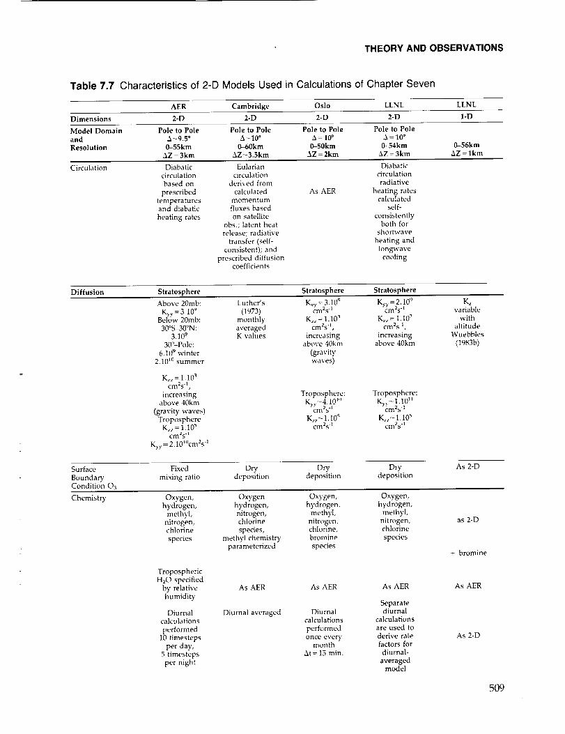
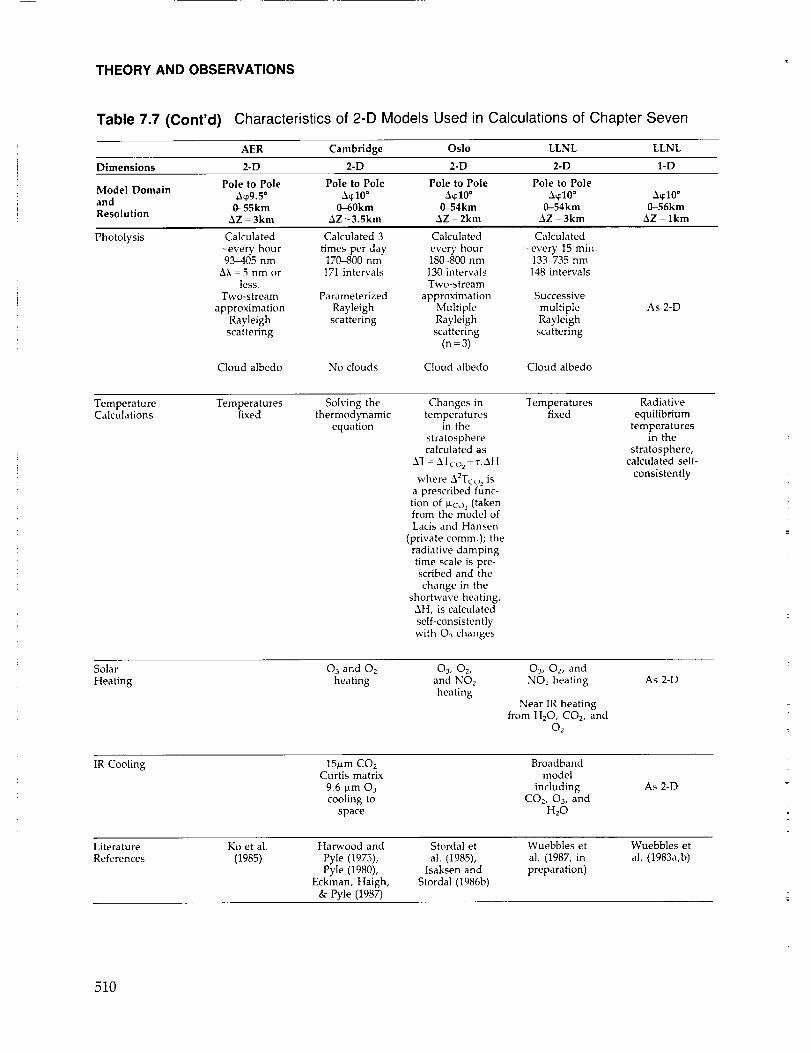
The present work is based on experiments with four different 2-D models (described in Table7.7) and with some parallel 1-D models. With the exception of the LLNL 2-D model, they were all

used in the previous compilation of model results. (See WMO 1986, Chapters 12 and 13, for a

more complete description of the types of 2-D stratospheric models and their performance.)

Three of the 2-D models (AER, LLNL, and Oslo) use a diabatic circulation, although their

transport velocities can differ because the circulations are derived from different data sets. In theAER and Oslo models, the circulation is fixed in all computations. In the LLNL model, the

temperatures are held fixed, while the radiative heating rates and the diabatic circulation arecomputed as ozone varies. The fourth 2-D model (Cambridge) uses a Eulerian circulation. The

mean transport by waves in the Cambridge model is represented as momentum fluxes based onsatellite observations and specified diffusion coefficients, and is held fixed while changes in the

508

THEORY AND OBSERVATIONS

Table 7.7 Characteristics of 2-D Models Used in Calculations of Chapter Seven

AER Cambridge Oslo LLNL LLNL

Dimensions 2-D 2-D 2-D 2-D 1-D

Model Domain Pole to Pole Pole to Pole Pole to Pole Pole to Pole

and A-_9.5 o A-10 o A = 10 ° A = 10 °

Resolution 0-55km 0--60kin 0-50km 0-54km 0-56kmAZ - 3km AZ-3.5km AZ = 2km AZ = 3km AZ = lkm

Circulation Diabatic Eularian Diabaticcirculation circulation circulation

based on derived from radiative

prescribed calculated As AER heating rates

temperatures momentum calcuIatedand diabatic fluxes based self-

heating rates on satellite consistentlyobs.; latent heat both for

release; radiative shortwave

transfer (self- heating and

consistent); and longwave

prescribed diffusion coolingcoefficients

Diffusion Stratosphere Stratosphere Stratosphere

Above 20rob: Luther's Kvv = 3.109 Kyy = 2.109 Kz

Kyy = 3.109 (1973) cm2s "l cm 2s-I variableBelow 20mb: monthly K,; = 1.103 K_; = 1.10 _ with

30°S-30°N: averaged cm2s% cm2s -_, altitude3.109 K values increasing increasing Wuebbles

30°_Pole: above 40km above 40kin (1983b)

6.109 winter (gravity2.10 l° summer waves)

K_ = 1.103

cm2s -I '

increasingabove 40km

(gravity waves)

TroposphereK;; = 1.105

cm2s -_

Kyy : 2.10_°cm2s -1

Troposphere: Troposphere:

Ky_4.10 I° Kyy_l.10 ]]cm2s -I cm2s -1

K,,_ 1,10 s K;,_ 1.10 scm2s_l cm2s 1

Surface Fixed Dry Dry Dry As 2-D

Boundary mixing ratio deposition deposition deposition

Condition O3

Chemistry Oxygen, Oxygen Oxygen, Oxygen,

hydrogen, hydrogen, hydrogen, hydrogen,

methyl, nitrogen, methyl, methyl,nitrogen, chlorine nitrogen, nitrogen, as 2-D

chlorine species, chlorine, chlorine

species methyl chemistry bromine species

parameterized species + bromine

Tropospheric

HaO specified

by relative

humidity

Diurnal

calculations

performed10 timesteps

per day,5 timesteps

per night

As AER As AER As AER As AER

Diurnal averaged Diurnal

calculations

performed

once everymonth

At = 15 min.

Separatediurnal

calculations

are used to

derive rate

factors for

diurnal-

averagedmodel

As 2-D

509

THEORY AND OBSERVATIONS

Table 7.7 (Cont'd) Characteristics of 2-D Models Used in Calculations of Chapter Seven

AER Cambridge Oslo LLNL LLNL

Dimensions 2-D 2-D 2-D 2-D 1-D

Pole to Pole Pole to Pole Pole to Pole Pole to PoleModel Domainand A_9"5° &_10° A_10° "X_10° A_10°

0--55km 0-60km 0-54km 0-54km 0-56kmResolution

AZ = 3kin AZ-3.5km AZ - 2km AZ - 3km AZ - lkm

Photolysis Calculated Calculated 3 Calculated Calculated

-eve O, hour times per day ever), hour -every 15 min.93-405 nm 170-800 nm 180-800 nm 133-735 nm

IX = 5 nm or 171 intervals 130 intervals I48 intervals

less. Two-stream

Two-stream Parameterized approximation Successive

approximation Rayleigh Multiple multiple As 2-DRayleigh scattering Rayleigh Rayleigh

scattering scattering scattering(n = 3)

Cloud albedo No clouds Cloud albedo Cloud albedo

Temperature Temperatures Solving the Changes in TemperaturesCalculations fixed thermodynamic temperatures fixed

equation in the

stratospherecalculated as

&T = &To 02 + "r. 3H

where A2Tco 2 is

a prescribed func-

tion of _co 2 (takenfrom the model of

Lacis and Hansen

(private comm.); the

radiative damping

time scale is pre-scribed and the

change in the

shortwave heating,AH, is calculated

self-consistently

with 03 changes

Radiative

equilibrium

temperaturesin the

stratosphere,calculated self-

consistently

Solar 03 and O2 03, 02, 03, O2, and

Heating heating and NO2 NO2 heatingheating

Near IR heatingfrom H20, CO2, and

02

As 2-D

IR Cooling 15_m CO2 BroadbandCurtis matrix model

9.6 p.m 03 including

cooling to CO2, 03, and

space H20

As 2-D

Literature

References

Ko et al.

(1985)IIarwood and Stordal et Wuebbles et

Pyle (1975), al. (1985), a]. (1987, in

Pyle (1980), Isaksen and preparation)

Eckman, Haigh, Stordal (1986b)

& Pyle (1987)

Wuebbles et

al. (1983a,b)

510

THEORY AND OBSERVATIONS

radiative transfer allow the circulation to change with ozone variations. The diffusion co-

efficients used for tracer mixing in the stratosphere are similar in the three diabatic circulation

models, and generally larger in the Eulerian model.

All of the models are based on same chemistry (DeMore et al., 1985); however, the Oslo model

is the only one to include bromine chemistry (held constant with time using background levels of

CHBBr). All the models assume the same values for the solar flux and compute photolysis rates ata number of different times during the day. Various techniques are used to include the effect of

diurnal variations in the chemical constituents.

Temperatures are calculated ab initio only in the Cambridge model, which calculates the

temperatures from the thermodynamic equation. The AER and LLNL models keep the tempera-

tures fixed in all computations. In the Oslo model, the temperatures in the stratosphere are

allowed to diverge from a reference value, thus allowing for a temperature feedback to the

chemistry. The assumption made in the Oslo model is that temperature changes are a purely

radiative adjustment in response to changes in solar heating, while the diabatic circulationremains unchanged. There is some evidence for this assumption from the 3-D GFDL model (Fels

et al., 1980). The LLNL model has employed the other extreme approach, namely that changes in

the heating rates are manifested purely as dynamical adjustment to circulation.

7.2.2 Basic Chemical Uncertainties

Uncertainties in perturbation calculations that are due to known measurement uncertainties

in reaction rate coefficients have been estimated for pure chlorine perturbations and for at least

one combined perturbation (Stolarski and Douglass, 1986; Grant et al., 1985). An important

result from such studies of error propagation is that combinations of rate coefficients that lead to

a very high sensitivity of ozone to chlorine give poorer results in matching observed atmosphericconstituents than do the models (i.e., combination of rate coefficients) with lower sensitivity to

chlorine (Douglass and Stolarski, 1987). The conclusion reached in that study was that acombination of chemical reaction rate coefficients that yields a sensitivity of ozone to chlorine

more than twice that calculated with the currently recommended rate coefficients is un-

satisfactory. The conclusion rests upon chlorine monoxide (CIO) being the rate-determining

radical for chlorine chemistry. The study is based on comparison of modelled and measured

trace species at midlatitudes and, further, does not include the heterogeneous chemistry

believed to be important in forming the Antarctic ozone hole.

Perhaps the most important facet of the chemical uncertainty is the question of completenessof the chemical mechanism. Early information on the atmospheric chemical mechanism was

derived from relatively high-pressure laboratory experiments in which many reactions were

occurring simultaneously. The reactions believed to be important were then isolated one at atime, and their reaction rate coefficients were measured. This process occurred over several

decades of careful laboratory experiments. Our present atmospheric chemical scheme is con-structed from these individually measured fundamental reaction rate coefficients.

In the early 1970's, many of the basic catalytic reactions had significant uncertainties in theirreaction rate coefficients. Progress in laboratory kinetics caused rapid changes in the evaluation

of perturbations. An example was the 1976 measurement of the NO + HOx reaction, whichfound a rate coefficient more than an order of magnitude larger than previous values (Howard

and Evenson, 1977). This led to model calculations of a lower stratosphere with significantly

511

THEORY AND OBSERVATIONS

more hydroxyl radical (OH) in which chlorine-catalyzed loss of ozone becomes more important.It is now believed that uncertainties in most of the major catalytic reactions and radical-radical

exchange reactions have been reduced to the order of 10-30 percent.

Another set of chemical uncertainties is associated with the major reservoir species such as

chlorine nitrate (CIONO2). Much of the present uncertainty in the calculated sensitivity of ozone

to chlorine or total odd-nitrogen (NOy) perturbations can be traced directly to the radical-

reservoir balance, which is determined by the formation and destruction processes for the

reservoirs. Many of the reservoir species are formed by three-body addition reactions, making

their chemical impact greatest in the lower stratosphere and at high latitudes. These locations areshielded from UV radiation by ozone absorption, yielding significant reservoir molecule life-

times, which in turn allow a buildup in their concentrations. The lower stratosphere and polar

latitudes thus may be the regions of greatest chemical uncertainty.

More recently, the question has been raised as to whether there might be very slowreservoir-reservoir reactions that return two reservoir molecules to radicals, thus significantly

enhancing radical chemistry and ozone destruction (WMO, 1986, Chapter 2). Laboratory

experiments have shown that the homogeneous gas-phase rate coefficients for reservoir-reservoir reactions are insignificant, but the possibility remains of a significant heterogeneous

contribution. This has, in fact, been suggested to be the mechanism for the rapid springtime

change in Antarctic ozone (see, e.g., Solomon et al., 1986a; McElroy et al., 1986b; Isaksen andStordal, 1986a; Crutzen and Arnold, 1986), where the surfaces for heterogeneous reactions are

believed to be the polar stratospheric clouds (PSC's). New laboratory studies indicate that

reservoir species containing chlorine are involved in this process. Observations of high C10

levels during periods with PSC's over Antarctica support this view (see the discussion in Chapter11). The critical role of heterogeneous processes for Antarctic ozone chemistry is now emerging

from a combination of atmospheric measurements, laboratory studies, and theoretical modeling

efforts; but its importance for the rest of the stratosphere is still under debate. Of particular

importance is understanding its role at high northern latitudes, where the meteorological

patterns are quite different from those found over Antarctica, and also at all latitudes in the lower

stratosphere after major volcanic eruptions.

As more and more laboratory studies are published, our confidence in the completeness of

the chemical mechanism for stratospheric ozone has increased. Except for the effects of het-

erogeneous chemistry, the past 5 years have seen little change in the evaluation of specifically

CFC perturbations.

7.2.3 Uncertainties in 2-D Model Transport

Significant advances have been made in the formulation of transport in 2-D models over the

past few years. For instance, it has been shown that 3-D general-circulation models can be usedto drive useful transport parameters for 2-D models (Plumb and Mahlman, 1987; Pitari and

Visconti, 1985). Nevertheless, there are still many problems that could affect our ability to model

changes in ozone: for example, only zonal mean processes can be explicitly described, and the

transport changes slowly with season or with latitude. Unfortunately, we know that theatmosphere is highly variable on all scales. Data for trace gas distributions will reflect this

variability; our models will not.

The rate of vertical advection coupled with the parameterization of eddy diffusion in the

stratosphere determines much of the calculated distribution of the long-lived trace species. The

512

THEORY AND OBSERVATIONS

estimated distribution of methane is of particular importance for the partitioning of the chlorine

species. A slow transport leads to lower concentrations of methane in the upper stratosphere,favoring a more efficient C1/C10 formation and thereby a more efficient ozone reduction by

catalytic chlorine reactions. Therefore, if the transport istoo slow in the models, the chlorine

effect is overestimated in the upper stratosphere. Comparisons of the calculated methanedistribution with observations in some of the model studies indicate that this might be the case.

However, the comparisons are not conclusive since the observations are also uncertain. SAMS

measurements of methane indicate large latitudinal gradients in the upper stratosphere such

that lower concentrations occur at higher latitudes. Models that duplicate this behavior (e.g.,

Solomon and Garcia, 1984a) and extend it to the polar regions (for which we are lacking

observations) show a high sensitivity of ozone to chlorine in this region because of the relative

absence of methane. This may be particularly important in assessing the latitudinal dependence

of perturbations.

Furthermore, some of the processes influencing ozone on short time scales are inherentlydifficult to model within a 2-D framework. This applies especially to the kind of dynamical

regime believed to exist in the Antarctic. An isolated vortex whose breakdown may well dependon ozone concentration is very difficult to model in two dimensions. Much of the transport

description in 2-D models is empirical and thus does not allow the kind of feedback processes

that may well be important in studying trends in ozone.

7.2.4 Comparison of Models With the Contemporary Atmosphere

The credibility of stratospheric models in predicting future ozone change will depend on howwell they reproduce current observations, particularly the distribution of key species directly

involved in ozone chemistry. Such tests of the models allow for ready intercomparison of models

and may help us understand any differences in the calculated scenarios for ozone, both past andfuture.

Because the chemistry of the stratosphere involves a nonlinear system of chemical reactions,

one should expect the results of perturbation calculations to be sensitive to the initial chemicalconcentrations, in particular that of Cly (total inorganic chlorine -- C1 + C10 + HC1 + HOC1 +OC10 4- C12 4- (C10)2 + C1ONO2). This is especially true for the NOx-Cly system, where the

reaction of C10 with NO and the reaction of C10 and NO2 to form C1ONO2 provide rapid

transition between regimes dominated by Cly- or NO×-catalyzed loss of ozone. This set ofchemical reactions has been shown to result in a rapid increase in ozone sensitivity to chlorine at

the level where Cly is approximately equal to or greater than the total odd nitrogen concentration

(e.g., Prather et al., 1984). For the current atmosphere, with Cly levels well below NOy levels, the

ozone depletion efficiency by chlorine reactions has been shown to increase with decreasing

NOy levels. A model with initial low NOy levels tends to give greater ozone depletion fromchlorine species than a model with high NOy levels (Isaksen and Stordal, 1986b). Thus, ourassessment of the effect of simultaneous changes in a number of species in the stratosphere

depends not only on the relative changes in each of the species, but also on the absolute

concentrations of many key species.

We have here selected a few key species to characterize the behavior of stratospheric

chemistry in the different models. Some of the models (Oslo, AER, and a previous version of the

Cambridge model) have been involved in a comparison study earlier (WMO, 1986). It is not theobjective here to make an extensive comparison of the different models used, but rather to apply

513

THEORY AND OBSERVATIONS

the most recent versions of the models and point out where significant differences occur. To

validate or to test more thoroughly these 2-D models, a more complete intercomparison of 2-D

models is planned as a separate task in the near future.

OzoJle

All of the models show some of the main features common to the observed latitude-height

distribution of ozone from the Limb Infrared Monitoring Spectrometer (LIMS) and the Solar

Backscatter Ultraviolet (SBUV) (see Figure 7.1). Theoretical altitude profiles for the tropics are

compared to a LIMS profile in Figure 7.2. The mixing ratio peaks above about 10 ppmv in the

Tropics at about 34 kin. The maximum calculated values range between 9 and 12 ppm in most

models, (in reasonable agreement with the LIMS values). All models overpredict O3 at 30 km and

underpredict it above 40 km. In the lower stratosphere, where ozone is controlled more by

dynamical transport, the mixing ratio surfaces slope poleward and downward due to the

predominant Brewer-Dobson circulation. In the models with the weakest horizontal diffusion(Oslo and LLNL), the slopes are steeper. In general, the models used here overpredict the peak

mixing ratio of ozone, and some of them place the maximum mixing ratios below those observed

by several kilometers.

There is a systematic discrepancy between observed and calculated ozone above 40 km, asdiscussed in WMO (1986). In the upper stratosphere, ozone is controlled by photochemistry, and

the discrepancy might indicate some important errors in modeling stratospheric chemistry.

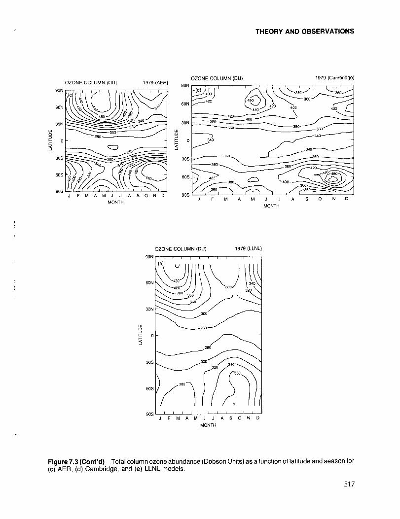
The integrated column abundance of ozone (often called total ozone) is shown in Figure 7.3 as

a function of latitude and time of year. Figure 7.3 shows TOMS observations along with resultsfrom all of the models. The main features in the observations are adequately described by the

models: low total ozone in the Tropics with little seasonal variation; increasing ozone column

with latitude; a maximum in the Northern Hemisphere at very high latitudes in late winter; large

seasonal variation at high latitudes; and a maximum in the Southern Hemisphere spring thatoccurs in midlatitudes rather than over the pole. The seasonal variation is suppressed in some of

the models (AER and Oslo), yielding too-high ozone columns in the summer and fall. In the

Southern Hemisphere, the maximum columns are observed at about 60°S in spring. While this

0.1

n_

wn-o.. 1o

10o90S

OZONE (ppmv) JAN 1979

(a)1 I I I I

-- LIMS V5.6.0 (A) -- SBUV 60

60S 30S 0 30N 60N 90N

LATITUDE

5O

4o(..9

wI

3O

OZONE (ppmv) JAN 1979 (Oslo)

4e- (b) 3.o.---__ k.

41_.- 6.0, _4:0_

7.0 - I- k I_N36 -- 8.0

_ 21

16

11

6

11 t 1 I I t I I80S 60S 40S 20S 0 20N 40N 60N 80N

LATITUDE

Figure 7.1 Ozone-mixing ratio (ppmv) as a function of latitude and altitude for January from (a) LIMS andSBUV observations for 1979, (b) Calculations using Oslo 2-D model.

514

THEORY AND OBSERVATIONS

5O

4O

LUO

3o

<:

LLI

__ 20>(0

Q.<

10

55

5O

45

4O

g as

_ 3025

15

10

OZONE (ppmv)

0.1

1

100

lO00 I I ] t90S 60S 30S 0 30N

LATITUDE

OZONE (ppmv)

10

I 060N 90N

JAN 1979 (Cambridge)

I _ I 3/ _a"r/ ' 1

_-3 _4-- _s_/__...___-.-- 4/_ 5.._. 6_6 _

0 I I I I90S 60S 30S 0 30N 60N 90N

LATITUDE

OZONE (ppmv) JAN 1979 (LLNL)

I i i i i i i i y_ i(e)

10

5

0 I I L I I I I ] I I90S 60S 30S 0 30N 60N 90N

100

i

i 1000

LATITUDE

J_giiitl,-

(/.)

ti-n

Figure 7.1 (Cont'd) Ozone-mixing ratio (ppmv) as a function of latitude and altitude for January from (c)Calculations using AER 2-D model, (d) Calculations using Cambridge 2-D model, (e) Calculations usingLLNL 2-D model.

515

THEORY AND OBSERVATIONS

Ev

LUa

b,<

51 I ,_ I t I 1 t I I t I I

os,o" s47 _'k_ Cambridge

45 - -,kx_..,_ AER43- ...... U_NL

".

39

37 JAN 1979 _i" "'_.",,

33- \

31 - / _.") )29 .... /_'"_ / /'

19 -_.'1/ -f I I I 1 I I I I 1 I

0 1 2 3 4 5 6 7 8 9 10 11 12 13

ppmv

Figure 7.2 Altitude profile of ozone-mixing ratios for January in the Tropics from LIMS observations and thefour 2-D models.

U.lt'_

OZONE COLUMN (DU)

90N

60N

3DN

30S

60S

90S

TOMS AVERAGE 1979-1986

J F M A M J J A S O N D

MONTH

I.gQ

f-l--5

OZONE COLUMN (DU) 1979 (Oslo)

60N

40N _ 330 _--_J_ 3'_0 "-''-'''_'-

_ 25

_270_ ?.90_2os _1_4os _31o_ j 3_o

J M M J S N J

MONTH

Figure 7.3 Total column ozone abundance (Dobson Units) as a function of latitude and season for (a)TOMS observations averaged 1979-1986, and (b) the Oslo models.

516

. THEORY AND OBSERVATIONS

OZONE COLUMN (DU)

90N

60N

30N

30S

60S

9OS

1979 (AER)

,°,::"i' ' ' ' ' ' ' * ' '

-----._=o_

F M A M J J A S 0 N D

MONTH

OZONE COLUMN (DU)

90N

60N

3ON

w0

---- o

30S

60S

90S

1979 (Cambridge)

t i , p L - _ I _ i /

__._ 420 _ _- _ _-- 400 _ /

34°_

J F M A M J J A S 0 N D

MONTH

90N

60N

30N

L,U,mz3_- o

i

30S

60S

90S

OZONE COLUMN (DU) 1979 (LLNL)

I I I I I I I I I I I

\ )l!!

J g M A M J J A S O N D

MONTH

Figure 7.3 (Cont'd) Total column ozone abundance (Dobson Units) as a function of latitude and season for(c) AER, (d) Cambridge, and (e) LLNL models.

517

THEORY AND OBSERVATIONS

maximum is found somewhat further poleward and later in the AER model, it is missing in the

Oslo model (see discussion in Stordal et al., 1985). The Cambridge model, on the other hand,

calculates ozone columns too high in the Tropics, as is expected from the high ozone mixing

ratios in the middle and lower tropical stratosphere (Figure 7.2). In the Northern Hemisphere,

the Cambridge model predicts maximum ozone columns at high latitudes during early summer,later than observed. As already mentioned, none of the models describes the Antarctic ozone

hole, which is apparent in the Total Ozone Mapping Spectrometer (TOMS) data covering1979-1986.

Odd Nitrogen (NOv)

One important issue brought up in previous 2-D model studies (WMO, 1986) was the

apparent lack of agreement between models and observations of NO× (LIMS observations of

nighttime NO2), particularly in the tropical lower stratosphere. Models tended to underestimatethe NO× present in this region. Large uncertainties in the NO× distribution strongly limit the

models' ability to predict ozone distribution, as ozone production from the CH4-NO× chemistry

at these heights is very sensitive to NO× levels. In the present diabatically driven 2-D models,

additional NOx is assumed to be produced by lightning, which is particularly efficient at high

tropospheric altitudes. This source is shown to have a pronounced effect on NO× levels in the

upper troposphere and lower stratosphere in equatorial regions (Ko et al., 1986). Another

possible mechanism that would increase NO× levels in the lower tropical stratosphere is

increased Kyy values, which would lead to increased transport of NOx into the Tropics frommidlatitudes.

Figure 7.4 is a latitudinal cross-section of NOy at three different pressure levels--3 mb (-40km), 16 mb (-30 km), and 30 mb (-25 km)--for July 1985. The figure shows that the present

models (Cambridge model not shown) agree fairly well with the observed data. The modelled

value for NOy falls within the range of the data from LIMS and ATMOS (Russell et al., 1988). The

NOy maximum in the three models ranges from 21 to 23 ppb, which is within the uncertaintylimits of the LIMS observations (Callis et al., 1985b).

The Oslo model has been used to study the impact of the lightning source of NO× on ozone

depletion. One scenario study has been performed both with and without the lightning source.

In the case that involved changes in trace gases only, the depletion of globally averaged totalozone from 1960 to 1980 was reduced from -0.7 percent to -0.4 percent when a lightning source

was introduced, as compared to a model without such a source; at the Equator, the ozone

depletion changed from -0.7 percent to -0.3 percent. For the period 1960-1990, the calculated

global decrease was reduced from - 1.4 percent to -1.0 percent. At high latitudes, ozone depletionis less sensitive to these NO× sources, decreasing from -2. I percent to -1.9 percent (March). The

uncertainties connected with the magnitude of the lightning source in the upper troposphere

(source strength, conversion to and removal of nitric acid (HNO3) leads to additional uncer-tainties in these calculations.

In the present model simulations, one source of change in stratospheric odd nitrogen is

included through the slow increase in the atmospheric concentration of nitrous oxide. Also

included are the changes due to variations in UV radiation over the 11-year solar cycle. Several

studies (e.g., Jackman et al., 1980; Garcia et al., 1984) have pointed out the potential forinterannual as well as 11-year solar-cycle variations due to mesospheric and upper stratospheric

production from energetic particles penetrating to these depths in the atmosphere. Callis and

Natarajan (1986) claimed that a significant increase in odd nitrogen occurred as measured bySAGE-II in 1985 as compared to SAGE-I in 1979. Other observations so far have not confirmed

the importance of such processes for variations in the ozone layer (see Chapter 9).

518

THEORY AND OBSERVATIONS

25

20

15

10

3mb I I I

, ..... "le.leow _

ATMOS "" =_-,44.:.

(a)

I I I

16S 32S 48S 64S

20

5

I I I

16mb

-- ._.." -

I I I

(b)

0 16S 32S 48S 64S

2O

15

10

5

I I I

30mb

- i .-...:._.._-_-.._.-.. • • -,.... -"_ • • ". • •J'/3"._.-..--'_-'.">-"" .....

_:_..._._

0I I I

(c)

16S 32S 48S

LATITUDE (APPROX.)

64S

LIMS DATA (SUMMER)

LLNL 1AER MODEL CALCULATIONS

....... Oslo

Figure 7.4 Total odd nitrogen (NOy in ppbv) as a function of latitude for summer from LIMS observationsand from the four 2-D models for (a) 3 rob, (b) 16 rnb, and (c) 30 mb. Also shown (crossed circle) are resultsfrom ATMOS.

519

THEORY AND OBSERVATIONS

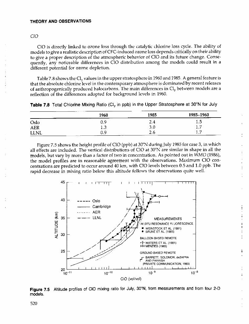
CIO

C10 is directly linked to ozone loss through the catalytic chlorine loss cycle. The ability of

models to give a realistic description of CFC-induced ozone loss depends critically on their ability

to give a proper description of the atmospheric behavior of C10 and its future change. Conse-

quently, any noticeable differences in CIO distribution among the models could result in a

different potential for ozone depletion.

Table 7.8 shows the Cly values in the upper stratosphere in 1960 and 1985. A general feature isthat the absolute chlorine level in the contemporary atmosphere is dominated by recent releases

of anthropogenically produced halocarbons. The main differences in Cly between models are areflection of the differences adopted for background levels in 1960.

Table 7.8 Total Chlorine Mixing Ratio (Cly in ppb) in the Upper Stratosphere at 30°N for July

1960 1985 1985-1960

Oslo 0.9 2.4 1.5AER 1.3 3.0 1.7

LLNL 0.9 2.6 1.7

Figure 7.5 shows the height profile of C10 (ppb) at 30°N during July 1985 for case 3, in whichall effects are included. The vertical distributions of C10 at 30°N are similar in shape in all the

models, but vary by more than a factor of two in concentration. As pointed out in WMO (1986),

the model profiles are in reasonable agreement with the observations. Maximum C10 con-

centrations are predicted to occur around 40 km, with CIO levels between 0.5 and 1.0 ppb. The

rapid decrease in mixing ratio below this altitude follows the observations quite well.

45

40

E35

LU

L_ 30<

25

i I i I IF_F i- I 1 I _ I _ I I _ I Illirl I Illl

\.

i ", I-_ .... os,oCambridge

........ AER

- LLNL / MEASUREMENTS -/

//[ .'IN SITU RESONANCE FLUORESCENCE

• WEINSTOCK ET AL. (198t)

• BRUNE ET AL, (1985)

BALLOON-BASED REMOTE

/[ " ÷ WATERSETAL,(1981)

('O') MENZIES (1983)

GROUND-BASED REMOTE

r" BARRETT, SOLOMON, deZAFRAr AND PARRISH

(PRIVATE COMMUNICATION, 1985)

I I I I LilIJ. _ + 1 i t LLII I I I I 111I

10-1o 10-9 10-8

CIO (vol/vol)

Figure 7.5 Altitude profiles of CIO mixing ratio for July, 30°N, from measurements and from four 2-Dmodels.

520

THEORY AND OBSERVATIONS

7.2.5 Stratospheric Temperature Feedbacks

The temperature of the stratosphere is predicted to respond to changes in ozone, to increases

in CO2, and to volcanic aerosols, as well as to dynamical forcing through transport of heat. Over

the study period, the past 30 years, model predictions indicate that stratospheric temperature

changes associated with trace gases and the solar cycle are modest--a few degrees at most. These

changes in temperature will feed back upon the chemical kinetics that control the concentration

of ozone. The impact of including this feedback has been tested in the Oslo model. The 1979-1987

period corresponds to the most rapid decline predicted for ozone concentrations near 40 km. Theestimated temperature decrease in the upper stratosphere is shown in Table 7.9 for the two

solar-cycle cases over the 8 years. Inclusion of this decrease in temperature affects the predicteddecline in O3, reducing the depletion by approximately 20 percent (see also Table 7.10).

Table 7.9 Calculated Temperature Changes in 1985 vs. 1979 for Oslo Model, Case 3. Values Are

Given for July at the Equator

Alt (km) Large Solar Small Solar

Cycle Model Cycle Model

49 -2.40 K -1.61 K

47 -2.86 K -2.06 K

45 -2.94 K -2.18 K43 -2.84 K -2.08 K

41 -2.15 K -1.50 K

39 -1.44 K -0.93 K

37 -1.30 K -0.79 K

35 -1.10 K -0.63 K

In the detailed comparison of the ozone simulations with observations, it may be important to

include temperature changes caused by factors other than ozone. Temperature variations of a

few degrees in the stratosphere due to year-to-year changes in dynamics or volcanic aerosols

could have a significant effect on the modeled trend in ozone. The temperature record for this

period is insufficient, however, and the model studies have not included this effect and itsinfluence on ozone.

Estimated stratospheric temperature changes due to the increasing concentrations of CO2 to

date are small. Over longer time periods, however, looking into the next century, increases in

CO2 may have a more substantial impact on stratospheric temperatures. The effects of expected

changes in tropospheric climate are not included in current stratospheric models and also maylead to uncertainties in the predicted temperatures of the stratosphere in the 2I st century.

7.3 MODEL SIMULATIONS OF OZONE CHANGE

Calculations of the response of atmospheric ozone for the natural and anthropogenicvariations described in Section 7.1 were made with the 2-D numerical models described in

Section 7.2. The models were initialized with atmospheric conditions 1955 and integrated with

time for the 30-year period of the study. One of the models (Oslo) continued calculations until

1991, the expected maximum of the upcoming solar cycle. The calculated history of ozone fromthe three cases defined in Table 7.1 is used to examine the relative contributions of the different

geophysical forcings to changes in ozone over the study period.

521

THEORY AND OBSERVATIONS

All experiments have been examined two dimensionally both in space (ozone mixing ratios asa function of latitude and altitude) and space-time (ozone columns as a function of latitude and

time). In 2-D calculations, the effects of CFC releases might be easier to separate from natural

variations in specific regions of the atmosphere during certain seasons when the maximumeffects are calculated to occur (the CFC "fingerprint"). Most 2-D models indicate that ozone

depletion, as reflected in total ozone observations, is most pronounced at high latitudes duringthe winter and spring seasons. This analysis focusses on the period 1979-1985 because of the

ability to compare these calculations with available satellite ozone observations.

To understand the impact of the atmospheric nuclear test series, the latitudinal and globaldistributions of ozone during the 1960's are examined. Because the tests occurred at widely

varying geographical locations, the previous 1-D model investigations of the response of ozoneto nuclear tests would not have been adequate to define the latitudinal variation of the calculated

response. Of particular interest are the high-latitude tests, which would be expected to yield

local perturbations not representative of a global-averaged response. The perturbations intro-duced by the atmospheric bomb tests are expected to be negligible a few years after the bomb

tests are stopped; thus, changes after the late 1960's come from the response to solar UV

variations and possible changes induced by man's releases of trace gases (e.g., CFC's).

7.3.1 Calculated Total Global Variations

As discussed in Section 7.1, four 2-D models were used to simulate expected ozone variations

since 1960. Figure 7.6 shows the calculations from each of these models for the three cases givenin Table 7.1. The model calculations are shown as percent deviations of the total column of ozonefrom the 1970 value. All four models show similar decreases for perturbation case 1 (trace gases

only). The ozone change for this case is smooth, with a decrease of nearly 1 percent reached by1985 as compared to 1970. The initial decay in the AER model from 1960 to 1965 is a transient, dueto the start of the calculations in 1960 rather than 1955. The other models began their calculations

prior to 1960, and no transients from the initial condition appear in 1960.

The superposed solar cycle in perturbation case 2 has an amplitude of 1.5-2.0 percent in each

model, all of which used the large solar-cycle model (Heath and Schlesinger, 1984) defined in

Table 7.4. Use of the small solar-cycle model deduced from the Solar Mesospheric Explorer

(SME) measurements (also Table 7.4) leads to a solar-cycle-induced amplitude somewhat less

than half of that shown in Figure 7.6 (0.7 percent for the Oslo model).

The atmospheric nuclear tests of the early 1960's are superposed in Figure 7.6 for perturbationcase 3. These occurred at a time of minimum expected ozone during the solar cycle. The bomb

effects are predicted to have disappeared by the late 1960's.

Also shown for comparison to these globally integrated 2-D models are results for per-turbation case 1 (trace gases only) for the AER 1-D model. That model was run for exactly the

same conditions as the 2-D counterpart. The 1-D model shows considerably less ozone depletion

since 1970, -0.2 percent at most. Similar differences between 1D and 2-D models are observed inthe LLNL models. Thus, we find that 1-D models cannot be used to calculate even the globally

averaged change in stratospheric ozone.

522

THEORY AND OBSERVATIONS

1.0 f I I I I I I I I I I I

h,' ' ' ' ' t "°TRACE GAS1.2 a) 294 0 ._"'-" ONI'Y- -' _

° :F--T7.... - t,5 -o . $ _ -20

_ -12 .... o _ -ao

I Y -1/ .........oo.. e_ CE GAS ÷ U_LT

SCENARIOS 1,2,3 w _T

_..oI ,..,,.: i I/EENNAARIoOs _ SO_, 284-2.4

II -5,0 _ _1 I I ! I

56 60 65 70 75 BO 85 60 62 64 66 68 70 72 74 76 78 80 82 B4

YEAR YEAR

-1 ¸

;_ -2uJ_j

_-3

-4

-5

(c) I I I I l I I

I __ "CASE21:il:3:

U -4

IZL

tfl

tII

f CASE 1 -- TRACE GASES ONLY

CASE 2 -- TRACE GASES + SOLAR CYCLE

t CASE 3 -- TRACE GASES + BOMBS

'lV CASE 3

I I J I )

65 7O 75 80 85

YEAR

-6

1 I I t I I i I

I ! \

I I

\/V

NH AVG (TRACE GASES)

NH AVG (SOLAR CYCLE _ TRACE GASES)

NH AVG IFULL SERIES)

86

-6 I I -8 I • I / t / I I

50 55 6O 90 50 54 58 62 66 70 74 78 82 86

YEAR

Figure 7.6 Timeline of percent change in globally averaged column ozone from model calculations for thethree cases described in Table 7.1 : (1) trace gas emissions only, (2) trace gases plus solar cycle, and (3) tracegases, solar cycle, and atmospheric nuclear tests for the (a) Oslo, (b) AER, (c) Cambridge, and (d) LLNLmodels.

7.3.2 Atmospheric Nuclear Tests

The nuclear bomb tests during the late 1950"s and early 1960's, with their associated injection

of large amounts of nitrogen oxides into the stratosphere, provide a possibility of testing some

aspects of the chemistry/transport models of the stratosphere. The model simulations of this

period are based on the emission scenarios given in Section 7.1.3. As seen in Figure 7.6, all fourmodels show a substantial depletion of total ozone during the year following the large explosions

in late 1962. The globally averaged decrease was substantially different in the four models, with

maximum yearly decreases ranging from 1.3 percent (Oslo) to almost 4.5 percent (Cambridge).The probable cause of this difference is the transport formulation in the models, since the bomb

tests are predominantly released at high northern latitudes. Figure 7.7 shows total ozone

depletion following the bomb tests in 1962 with time and latitude as calculated by the LLNL

model; the model estimates total ozone to have dropped by 56-68 DU (Dobson Units) at 70°N.

A depletion of similar magnitude has been reported for observations of total ozone from the

Dobson network (Reinsel, 1981; Angell et al., 1985; Bojkov, 1987) (see Figure 7.10). However, the

observed depletion tends to start well before the time predicted by the models. This discrepancy

523

THEORY AND OBSERVATIONS

WO

I--<.J

90N

60N

30N

30S

60S

90SJ F MA M J J ASO N D J FMA M J J D J

1962 1963

Figure 7.7 Calculated change (%) in column ozone changes as a function of time and latitude during theatmospheric nuclear tests. Results from the LLNL 2-D model are shown for 1962-1963.

could have many causes, including the limited geographic representativeness of the early

Dobson network. Until the reasons for the discrepancy are better understood, it is difficult to

draw conclusions from this comparison regarding the ability of the models to simulate the

atmospheric test series.

We have studied the sensitivity of the above results to moderate differences in the scenario

for NO generated by the atmospheric nuclear tests. The difference between a simulation using

the reduced set of bomb tests (Table 7.6) and one using the full set, including the smaller bombs,

is of the order of 10 percent for the Northern Hemisphere average, the full set giving the larger

depletion (LLNL model). A similar comparison using the Oslo model yielded even smaller

differences. Based on these considerations, we estimate that the bomb tests are likely to have

produced an ozone depletion at high northerly latitudes in early 1963 of 25-75 DU. Thecorresponding range for the global average depletion is 3-15 DU. These estimates should be

regarded as tentative, as there still are uncertainties connected to the models.

The absolute magnitudes of the calculated ozone depletion depends, among other things, on32

the adopted emission scenario for NO. The assumption of I x 10 molecules of NO produced by

each MT total yield of nuclear explosion, as used in the AER, Oslo, and Cambridge simulations,

is probably uncertain by at least a factor of two (see discussion in Section 7.1.3).

As seen in Figures 7.6 and 7.7, the recovery time of the depletion following the major

explosions is a few years. Five years after the major injection in late 1962, very little depletionremained. This is a feature common to all models.

524

THEORY AND OBSERVATIONS

7.3.3 Column Ozone: Comparison With Observations

The primary long-term data set that is available for comparison to model calculations is thatfor total ozone from the ground-based Dobson spectrophotometers. Approximately 30 years of

data can be used for trend analysis. Satellite data give a better global coverage of ozone

distribution but are available only from late 1978. In the following sections, ozone trendscalculated with the four 2-D models will be compared with ozone trends deduced from the

Dobson network. An example using data from the TOMS instrument on Nimbus-7 will also be

used for comparison. The emphasis of these studies is to search for fingerprints from theoretical

models that can use existing measurements to separate the changes due to solar cycle from those

due to trace gases.

7.3.3.1 Theoretical Fingerprints for Solar Cycle and Trace Gases

We present two separate model calculations covering the period from solar maximum in 1979to solar minimum in 1985: solar-cycle effects and concurrent changes in trace gases.

Calculated ozone changes due to solar-cycle effects alone are shown in Figure 7.8 for one

model (Oslo), using the large solar-cycle case in Table 7.4. The main feature, which is the samefor all four models, is the almost constant depletion of ozone with latitude and season ranging

from 1.7 percent to 2.1 percent (Oslo model) going from solar maximum to solar minimum. For

the small solar-cycle case, the Oslo model calculates ozone reductions of similar pattern, but

smaller magnitude--about 0.7 percent.

2

80N

60N

40N

20N

0

20S

40S

60S

80S

-2.00

3 5 7 9 11 13

MONTH

Figure 7.8 Calculated change (%) in column ozone from 1979-t985 as a function of latitude and monthfrom the Oslo model. The results demonstrate the effect of solar cycle (maximum to minimum) alone,neglecting all other influences.

525

THEORY AND OBSERVATIONS

The calculation for the same period, but with only trace gas changes included (case 1), is

shown in Figure 7.9. In contrast to the solar cycle case, all the models show distinct latitudinal

and temporal patterns of ozone depletion, with the largest changes occurring at high latitudesduring winter and spring (n.b., results from the Cambridge model were not available for this

figure; the Cambridge model is known to produce a quite different pattern at high latitudes for

trace-gas impacts on ozone). However, the magnitude of the depletion, a global average of order

0.3 to 0.6 percent over this period, is substantially less than that obtained for the solar-cycle

W0

I-

5

'I'(' '/' \'\

60N '_10 #// ) 1 -0

40N - • "

20S - _ -0,5o

608 -

(a)

80S I IJ F M A M J J A S O N D J

MONTH

90N I _ I i_ I. i --t I,,_j/ _l i • I I

6o _2_ o _-o.3--'_'_

605

90S I I I I I I i" "1 I I I

J F M A M J J A S O N D

MONTH

90N

60N

30N

30S

60S

90SJ

b

IIIII

FMAM

t I I t I I I

I l I i i I I

J J A S O N D

MONTH

Figure 7.9 Calculated change (%) in column ozone from 1979-1985 as a function of latitude and month,considering trace gases only (case 1). Calculations are from the (a) Oslo, (b) AER, and (c) LLNL models.

526

THEORY AND OBSERVATIONS

effects in the large solar-cycle case. If we compare with the case for small solar-cycle variations,

then trace gases become more significant, particularly at high latitudes.

The magnitude and phase of the solar cycle must be correctly taken into account in data

analysis for comparison with the models. For example, results from the AER model showed that

shifting the time period for comparison by I year (1978 to 1984) led to noticeable changes in the

calculated solar-cycle impact. Our current model for the solar-cycle variations is simplistic (a sine

curve), and future efforts will require a more realistic model scaled to solar activity, such as the

11-year pattern for sunspots or 10.7 cm flux.

7.3.3.2 Thirty Years of Dobson Data

Thirty years of total ozone observations have been reanalyzed by Bojkov (1987) and pre-

sented in Chapter 4 of this report. The data have been divided into latitude bands, based onstation location. The three latitude bands for which there were sufficient data to construct a

meaningful average are shown in Figure 7.10 (30-39°N, 40-52°N, 53-64°N). For each of these

latitude bands, calculations from the four models are superposed.

The observations show a distinct biennial oscillation, which is particularly pronounced at

high latitudes. This feature is not seen in the calculations for reasons that already have been

discussed. Also, there is an apparent solar-cycle variation that is broadly in agreement with the

calculated solar-cycle variation. However, any trends related to trace gas releases are difficult to

deduce from Figure 7.10 due to the large variability of the observations.

7.3.3.3 Global Data From Satellite, 1979-1987

A characteristic of the Dobson data presented for latitude bands in Figure 7.10 is its variability

on all time scales. Much of this variability is meteorological and can be removed by the more

complete coverage of satellite data available from late 1978. Even when satellite data are used to

integrate over large areas of the globe, however, significant variability remains. Figure 7.11shows one example using data from the TOMS instrument on Nimbus-7. The dots are the daily

values of the area-weighted integral of total ozone from 65°S to 65°N over the 9-year data record.

The point values are relative to the 9-year average for that particular week; the line through the

points is a 60-day running mean. Also shown by a heavy line is the annual average calculated by

the Oslo model, including both solar cycle and trace gas effects. The TOMS result is similar to

that previously presented by Heath (1988) for SBUV data, except in this case, the TOMS datahave been corrected as a function of time over the 9-year period by adjusting to the Dobson

record (i.e., using satellite overpasses and subtracting the mean difference between the two

records). As can be seen in the figure, the long-term changes in total ozone calculated by the

model are in general agreement with observations, but the data exhibit significant variability

relative to the long-term changes. It is not clear whether we should regard this failure to

reproduce the observed variability as a fundamental discrepancy between models and theory or,

more likely, as an inherent limitation in the 2-D nature of the models.

Additional information can be obtained from the seasonal and latitudinal behavior of the

change in total ozone, as shown in Figure 7.12 for TOMS data, where the difference between the

mean of the years 1985 plus 1986 and the mean of the years 1979 plus 1980 is plotted. The data

have been adjusted to account for the drift of TOMS with respect to Dobson overpasses. The

springtime Antarctic ozone hole is clearly visible, with changes of greater than 30 percent (see

527

THEORY AND OBSERVATIONS

4

3

2

w I

z 0<I

wo -3rruJa_ -4

-5

--6

-7

4

3

2

w 1

Z 0<I0 -1

I.-z -2LU

ILl

13.- -4

-5

--6

-7

4

3

2

w 1(9Z< 0-t-O -1f-

zw-20rr -3uJ_ -4

-5

-6

-7

' ' I ' I ' 1 t l I I I t

(a) 52N - 64N

/...... Oslo

....... AER

Cambridge

I I I 1 I I t 1 I I I I I I I I I I I

66 68 70 72 74 76 78 80 82 84

YEAR

• I i i_ 1 t [ i I i I I I t I I

(b) 40N- 52N

.... _'---'-T-._-_'"-.

.%

Oslo V

....... AER

--.- Cambridge

I I I I [ I l I I I I I I I I I I I 1

66 68 70 72 74 76 78 80 82 84

YEAR

p t t _ I ' ' ' i I ' _ ' ' I ' J

(c) 30N- 40N

,.

_ Observations (Bojkov)..... Oslo

....... AER

----- Cambridge

I I I I _ i I I I t I I I I J I I t I

66 68 70 72 74 76 78 80 82 84

YEAR

Figure 7.10 Timeline of percent change in column ozone from 1965 to 1985 for the latitude bands (a)52-64°N, (b) 40-52°N, and (c) 30-40°N. Reevaluated data from the Dobson network (see Chapter 4) areshown by the thick line. Calculations from three models (Oslo, AER, and Cambridge) are also shown forcomparison.

528

THEORY AND OBSERVATIONS

zLU0trLUEL

(nZo

_f

a

2

0

-2

-4-

-6

78

I I I I I I I f 1 I

.... . ,.:,4: _..;L_ OSLO

__,.....".':'.";,':';''"';__.::_l" s;''P: ;_" ;...._ __'__"" _:''_',.,' . ['.: _' ._MODEL--_;_!,_..',_'_"___ _

•_ :_ _ ; -.:- ,:._•. : ¢"=_

l I I I I I I I I I79 80 81 82 83 84 85 86 87 88 89

YEAR

Figure 7.11 TOMS data for column ozone integrated from 65°S to 65°N are shown for 1978-1987. TheTOMS satellite data have been normalized to the ground-based Dobson network. The points representpercent deviations of the daily average from the 9-year average for that particular week; the thin solid line is a80-day running mean through the points. The thick solid line shows calculated total ozone (Oslo model) forthis period.

ILlO

I-"-

F-<_J

70N -%

50N

30N

_os

50S

90SJ F M A M J J A S O N D

MONTH

Figure 7.12 Observed change (%) in column ozone from TOMS data, the average of 1985-1986 minus theaverage of 1979-1980. The TOMS data have been recalibrated and do not reflect the currently archived data:TOMS data for 1985 and 1986 have been increased by approximately 4 percent to account for drift withrespect to Dobson network.

529

THEORY AND OBSERVATIONS

Chapter 11). In addition to this primary signal, the data also show noticeable depletions at highlatitudes in late fall, winter, and early spring. This pattern is closer to the calculated fingerprint

for trace gases than it is to that for the solar cycle (see Figures 7.8 and 7.9). There is a possible

indication from these TOMS data that the magnitude of the decrease in the winter at high

latitudes may be more pronounced than that calculated in the models.

Calculations of the combined effects of trace gases and solar cycle from 1979 to 1985 are shown

in Figure 7.13 as a function of latitude and season. The predominant change is a global net

80N

60N

40N

2DN

ILl

EQ

,_1

20S

40S

60S

80S

uJrl

I-

.J

90N

60N

30N

EQ

30S

60S

90S

OSLO

( t )/dJ F M A M J J A S O N D

MONTH

(a)CAMBRIDGE

t _ I " t t _ l I I 1 I

_,-1,75_ - "

-.-1,50

-1.

I I I I I I l I I. I I

J F M A M J J A S O N D

MONTH

(c)

90N

60N

30N

uJa

i- EQI.-<_J

30S

60S

90S

AERI I I ,l I I I I I_ I I

-25_

F M A M J J A S O N D

MONTH

(b)LLNL

90N t I I i i i i t i i i

60N __2.7_,, 2.50 \ ,/

/30S -_ -_.50 -2_75 -2.5o

-2.?

90S I I I I I I I I I I IF M A M J J A S O N D

MONTH

(d)

Figure 7.13 Calculated change (%) in column ozone as a function of latitude and season from 1979-1985,including effects of trace gases and solar cycle. Calculations are from the (a) Oslo, (b) AER, (c) Cambridge,and (d) LLNL models.

530

THEORY AND OBSERVATIONS

decrease of order 1.5 to 2.5 percent that is associated with the solar cycle, and a smaller influence

of the trace gases that is superimposed. Three of the models show similar variations, with largest

decreases at high latitudes during winter, but the Cambridge model gives a markedly different

result with ozone increases as large as 0.5 percent at high latitude during summer. The cause of

this difference is not yet understood.

7.3.3.4 Subtracting the Solar Cycle From Dobson Data

One way to separate the solar cycle and trace gas effects is to use the Dobson data over two

complete 11-year solar cycles. Bojkov (1987) in Chapter 4 has done this by comparing the records

during two different seasons for two ll-year averaging period: 1965-1975 and 1976-1986. Figure

7.14 shows the difference between these ll-year records for the summer season (May-August)

and the winter season (December-March) from each of 36 stations that are plotted as a function

of station latitude. The summer season differences are small and consistent with the two model

calculations, also shown in Figure 7.14. Decreases during the winter season are pronounced, and

generally much larger than the model predictions, particularly north of 30°N. Model calculations

w

z<"I-0

Zw0nnLUO-

2

1

0

-1

-2

-3

-4

-510N

I I io

(a)o% SUMMER

oo o

o o o 9o _

---?t-- -oo° o

O o OBSERVATIONSO

Oslo MODEL

--=-- AER MODEL

I L I

30N 50N 70N

LATITUDE

w(.9 0

I-z -2LU(OrruJ -3(:1.

-4

-510N

I I I

(b)o WINTER

_ - o_.,,:0

0 0

00 0

o_

o OBSERVATIONS O

Oslo MODEL o d 3

--m-- AER MODEL

I _ O I

30N 50N 70N

LATITUDE

Figure 7.14 Observed change (%) in column ozone between the 11-year (solar-cycle) averages1965-1975 and 1976-1986 for (a) summer season (May-June-July-August) and (b) winter season (De-cember-January-February-March). Points representing values from single stations are plotted as a functionof station latitude. Results from two 2-D models (Oslo and AER) are also shown.

531

THEORY AND OBSERVATIONS

(AER and Oslo) are in qualitative agreement with observations in that depletion increases

toward higher latitudes, but the magnitude of the decrease predicted near 50°N (about -1

percent) is substantially less than that observed (about -1.5 to -4.5 percent).

If the similar feature seen in the TOMS data for 1979-1986 is robust (i.e., survives the current

recalibration of the data set), then it is likely that current 2-D models underestimate the decreases

in total ozone that have occurred at high northern latitudes over the last one to two decades. It is

difficult at present to explain the cause of this discrepancy; however, it may be that the present

2-D models are missing some chemical processes, quite possibly heterogeneous chemistry that is

particularly important at high northern latitudes, similar to that associated with the Antarcticozone hole.

7.3.4 Profile Ozone: Comparison With Observations

We now examine the model-calculated changes in the local concentrations of 03 as a function

of latitude and altitude; we hope to associate different patterns of change with the geophysical

forcing included in the models: trace gases, solar cycle, and atmospheric nuclear tests. This

analysis will concentrate on the calculated differences between 1979 and 1985 (solar maximum tosolar minimum). For this period, we have global data from satellites (SAGE-I and SAGE-II,

SBUV) and limited coverage from ground-based observations (Umkehr). We focus on small

percent changes in the vertical profile of ozone concentrations and look for latitudinal effects.

7.3.4.1 Fingerprints of the Solar Cycle and Trace Gases

Ozone perturbations induced by the solar cycle alone (1979-1985, maximum-to-minimum,

no trace gas changes) as calculated by the models are shown in Figure 7.15a as a function of

height and latitude. Solar flux changes for the large solar-cycle model are used in thesecalculations. The decrease in UV intensities leads to decreases in stratospheric ozone at all

latitudes and altitudes. The models predict a broad maximum around 40 km, with ozone changes

between -1.5 and -3.0 percent. Calculations with the small solar-cycle model give a similar

pattern, but with substantially smaller ozone perturbations. A characteristic pattern for thesolar-cycle-induced changes is that the latitudinal gradients are moderate at all altitudes.

The calculated changes in 03 concentrations between July 1979 and July 1985 for case 2 (trace

gases plus solar cycle) are shown in Figure 7.15b-e for all four models. Ozone changes in the

upper stratosphere (1-3 mb, 48-40 km) are dominated by the effect of chlorine increases rather

than solar cycle (compare Figure 7.15a with 7.15b). The effect of trace-gas changes has a

pronounced latitudinal pattern and is approximately twice as large as that from the solar cycle.Maximum depletion of ozone occurs about 2 mb (43 km) and ranges from -7 + 2 percent in the

Tropics to -10 + 2 percent at mid- and high latitudes. From 1979 to 1985, the models predictdecreases in stratospheric ozone at almost all latitudes and altitudes, the one exception being the

Cambridge model, which predicts increases in the high-latitude lower stratosphere during

summer. The upper stratosphere is, therefore, an area where the impact of CFC's can be more

readily detected, as the trace-gas effects dominate the solar cycle for the period 1979 to present.

Results from all models show similar morphology in the upper stratosphere, although there

are some differences near the winter pole. These variations may indicate the different way in

which models treat the chemistry near the polar night, or may reflect differences in stratospheric

transport at high latitudes. The magnitude of the maximum calculated change is almost twice as

large in polar regions relative to the Tropics in three of the four models, whereas the LLNL model

532

THEORY AND OBSERVATIONS

OZONE CONCENTRATION (PERCENT CHANGE)

JUL 1985 vs 1979 (Oslo: Solar cycle only)

f_ _.1 I I I I I

41

16

11

(all I

80s 60s 40S 20s 0 20N 40N 60N 80N

LATITUDE

OZONE CONCENTRATION (PERCENT CHANGE)JULY 1985 vs 1979 (Oslo)

45

41

g 33_ 292 25

_, 21

13 o

9

5

180S 60S 40S 20S 0 20N 40N 60N 80N

LATITUDE

100

lOO090S

OZONE CONCENTRATION (PERCENT CHANGE)JULY 1985 vs 1979 (AER)

.1 I I I I I

_ /_o_ '-_________-

-1 __i

:-IcI---T--o_' i , °'n----'-60S

65

6O

55

5O

45

4og35 _3o 2

25 ._20

15

10

5

030S 0 30N 60N 90N

LATITUDE

30

_' 20<

10

OZONE CONCENTRATION (PERCENT CHANGE)JULY 1985 vs 1979 (Cambridge)

5O

40- ____._____._.._ _1 _-- -_-_ _4 _

._-_f __

0 (d)_ll -_ __L__ I I

90S 60S 30S 30N 60N

uJ

100

0

LATITUDE

100090N

OZONECONCENTRATION(PERCENTCHANGE)JULYI985vsI979(LLNL)

Figure 7.15 Calculated height-latitude changes (%) in ozone from July 1979 to July 1985 for solar cycleonly from the Oslo model (a), and solar cycle plus trace gases (case 2) from the (b) Oslo, (c) AER, (d)Cambridge, and (e) LLNL models.

533

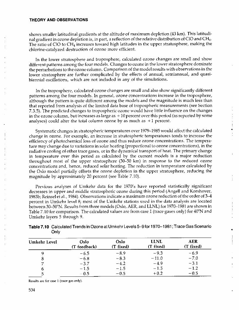
THEORY AND OBSERVATIONS

shows smaller latitudinal gradients at the altitude of maximum depletion (43 km). This latitudi-

nal gradient in ozone depletion is, in part, a reflection of the relative distribution of C10 and CH4.

The ratio of C10 to CH 4 increases toward high latitudes in the upper stratosphere, making the

chlorine-catalyzed destruction of ozone more efficient.

In the lower stratosphere and troposphere, calculated ozone changes are small and show

different patterns among the four models. Changes to ozone in the lower stratosphere dominate

the perturbations to the ozone column. Comparison of the model results with observations in the

lower stratosphere are further complicated by the effects of annual, semiannual, and quasi-

biennial oscillations, which are not included in any of the simulations.

In the troposphere, calculated ozone changes are small and also show significantly different

patterns among the four models. In general, ozone concentrations increase in the troposphere,

although the pattern is quite different among the models and the magnitude is much less than

that reported from analysis of the limited data base of tropospheric measurements (see Section

7.3.5). The predicted changes to tropospheric ozone would have little influence on the changesin the ozone column, but increases as large as + 10 percent over this period (as reported by some

analyses) could alter the total column ozone by as much as + 1 percent.

Systematic changes in stratospheric temperatures over 1979-1985 would affect the calculated

change in ozone. For example, an increase in stratospheric temperatures tends to increase the

efficiency of photochemical loss of ozone and thus reduce ozone concentrations. The tempera-

ture may change due to variations in solar heating (proportional to ozone concentrations), in theradiative cooling of other trace gases, or in the dynamical transport of heat. The primary change

in temperature over this period as calculated by the current models is a major reductionthroughout most of the upper stratosphere (30-50 km) in response to the reduced ozone

concentrations and, hence, reduced solar heating. The reduction in temperature calculated by

the Oslo model partially offsets the ozone depletion in the upper stratosphere, reducing the

magnitude by approximately 20 percent (see Table 7.10).

Previous analyses of Umkehr data for the 1970's have reported statistically significant

decreases in upper and middle stratospheric ozone during this period (Angell and Korshover,1983b; Reinsel et al., 1984). Observations indicate a maximum ozone reduction of the order of 3-4

percent in Umkehr level 8; most of the Umkehr stations used in the data analysis are locatedbetween 30-50°N. Results from three models (Oslo, AER, and LLNL) for 1970-1981 are shown in

Table 7.10 for comparison. The calculated values are from case I (trace gases only) for 40°N and

Umkehr layers 5 through 9.

Table 7.10 Calculated Trends in Ozone at Umkehr Levels 5-9 for 1970-1981 ;Trace Gas Scenario

Only

Umkehr Level Oslo Oslo LLNL AER

(T feedback) (T fixed) (T fixed) (T fixed)

9 -6.5 -8.9 -9.3 -6.9

8 -6.8 -8.3 -11.0 -7.0

7 -3.7 -4.2 -4.9 -3.1

6 -1.5 -1.5 -1.5 -1.2

5 -0.5 -0.5 +0.2 -0.5

Results are for case 1 (trace gas only).

534

THEORY AND OBSERVATIONS

Results from the different models compare well in the lower layers, but there is a significant

difference in layers 8 and 9, where the LLNL model gives the largest .calculated change in ozoneover 1970-1981. We are unable at present to explain these differences and await a more complete

model intercomparison. Calculations with the University of Oslo model were done with fixed

temperatures and with a parameterization for the change in temperature due to increased CO2

and changes in O3. As noted above, temperature feedback is important in calculating ozone

change, particularly in the upper stratosphere, layers 7, 8, and 9. Although in qualitative

agreement with observations, all models give calculated changes in ozone in Umkehr levels 8

and 9 that are substantially larger than those determined from analysis of Umkehr data; the

comparison is better at the lower levels.

All models show that the upper stratosphere is the altitude region most sensitive to trace gas

releases, and that the magnitude of the effect exceeds effects introduced by solar-cycle vari-

ations. The models also predict strong latitudinal gradients due to increases in trace gases, in

contrast to the impact of the solar cycle. Therefore, the upper stratosphere is the region where it

should be possible to identify the fingerprints of trace gases on ozone. Such identification,

however, will depend critically on the quality and global representation of the observations.

7.3.4.2 Trends in Vertical Structure, 1979-1985

Figure 7.16 compares the changes in the altitude profile of ozone from SAGE-I (1979-1980) to

SAGE-II (1984-1985, latitude belts 20-50°N and 20-50°S) and from the Umkehr network (stations

55

50

45A

E

"" 40IJJ

I--- 35I-._1.<

30

25

OZONE CONCENTRATION

I t I

,_i_i__:_:_:_

D,- = [] /_

,98 -5 .us , 79-80\%

- []MODEL 1985 MINUS 1979 r-A

[]UMKEHR 1986 MINUS 1979

r_v,

20 I I 1 I I-20 -15 -10 -5 0 5 10

PERCENT CHANGE

Figure 7.16 Observed changes (%) in stratospheric ozone profiles from different instruments over1979-1986. Differences between SAGE-I (1979-1980) and SAGE-II (1984-1985) measurements areshown for northern and southern latitudes (20°-50°). Umkehr observations from 1979-1986 are limited tonorthern midlatitudes. The band shows the range of model calculations (1979-1985, midlatitude, Oslomodel) for both large and small solar-cycle models.

535

THEORY AND OBSERVATIONS

between 36°N and 52°N) to the calculated change in ozone profile from the Oslo model

(midlatitudes). Analysis of Umkehr data for trends during 1979-1986 is complicated by the

strong interference of aerosols following the E1 Chich6n eruption. One recent report, however,claims that it is possible to correct partially for this interference and, thus, to deduce upper

stratospheric ozone changes over this period (see Chapter 5).

Both observations and models show ozone depletions that increase with altitude, peaking

around 40-45 km. The calculated depletion in the upper stratosphere is larger than that reported

from the SAGE observations, but slightly smaller than that from the Umkehr analysis. The

discrepancy with the SAGE data is most pronounced around 50 km, where observations show a

slight ozone increase. However, there is a possible systematic difference in derived ozone valuesbetween the two SAGE instruments that may be as large as -+4 percent (see Chapter 5). The scale

on the SAGE curve in Figure 7.16 could be shifted by as much as 4 percent, bringing the

observations into better agreement with the calculations between 30 and 45 km, but still not

explaining the small change above 45 km or the significant depletion below 30 km. Similarly

enhanced ozone depletion in the lower stratosphere is deduced from ozonesonde data for thelast two decades over Germany (Bojkov and Attmanspacher, 1988); however, changes of this

magnitude in the lower stratosphere should be clearly evident in the total ozone column--and

this is not apparent from the ozone column data.

The currently archived SBUV data for the same period show ozone depletions that are

substantially larger than the models or data shown in Figure 7.16 and that have a distinctly

different profile: a maximum ozone depletion of approximately 20 percent is found at 50 km. Itis believed that these data cannot be used to determine changes in the ozone profile (see

Chapter 5).

7.3.5 Tropospheric Ozone

7.3.5.1 Impact on Column Perturbations

Although only about 10 percent or less of the total ozone column is located in the trop-

osphere, increases in tropospheric ozone that have occurred over the last few decades might

have produced a detectable change in the ozone column. Therefore, observed trends in total

ozone must not be interpreted uncritically as reflecting stratosphere changes alone. Similarly, it

is important for models to include tropospheric processes in a realistic way if they are to attempt

to simulate changes in total ozone.

There are indications that the ozone levels in surface air are substantially higher in the present

atmosphere over Europe and the U.S. than those found during the end of last century (Bojkov,

1986c; Kley et al., 1988), and that, during the last two decades, an increase of -1 percent per year

has taken place in the free troposphere over most of the observing sites in the Northern

Hemisphere (Bojkov, 1988b). Measurements over the last 30 years show substantial increases,

-50 percent, during this period at surface levels over East Germany (Warmbt and Feister, 1984).The increases are not confined to the planetary boundary layer, but are observed also in the free

troposphere. Ozone increases are observed to be largest northward of 40°N, with stronglatitudinal dependence. Increases are particularly large over and around industrialized areas in

Europe and North America (Logan, 1985). For example, ozonesonde observations over West

536

THEORY AND OBSERVATIONS

Germany (Bojkov and Attmanspacher, 1988) report increases much larger than 1 percent per

year throughout the troposphere over the last 20 years.

Assuming that the reported increases in tropospheric ozone, -1 percent per year, are

representative of average conditions throughout the Northern Hemisphere for the last twodecades, we can estimate the impact on the total ozone column. Tropospheric ozone should have

produced an increase in column ozone of about I percent from 1970-1985 and about 0.5 percentfrom 1979-1985. Increases over industrialized areas would have been substantially greater, but

these areas are a small fraction of the hemisphere. Therefore, the observed downward trend in

total ozone at most northern sites might actually be larger than measured, being partially

compensated for by increases in tropospheric ozone.

7.3.5.2 Uncertainties in the Estimates

The observed increase in tropospheric ozone is likely caused by anthropogenically induced

increases in the concentration of precursor gases NO×, CH4, nonmethane hydrocarbons

(NMHC), and CO, although quantitative estimates are connected with large uncertainties (e.g.,Isaksen and Hov, 1987). A main uncertainty in modelling tropospheric ozone comes from our

lack of knowledge of NO× distribution in the troposphere. Due to short chemical lifetime (days or

less) and uneven source distribution, NO× shows strong temporal and spatial variations in the

troposphere. The efficiency of the CH4-NO× chemistry for ozone production is strongly and

nonlinearly dependent on NOx levels, and the 2-D formulation of the current models is limited in

representing the spatial variations in tropospheric NO×. Additional uncertainties in ozone

production and trends in the troposphere are introduced by our lack of knowledge of long-termtrends in CO, NMHC, and NOx.

The 2-D models used in this study all have a very crude representation of tropospheric

processes. They do, in general, predict an increase in tropospheric ozone during the last two

decades, but this increase is global and not limited to the northern midlatitudes, for which

observations indicate substantially larger increases. Production of tropospheric ozone in the

Northern Hemisphere may be underestimated because the models do not include any trends inshort-lived anthropogenic species like CO, NOx, and NMHC. According to model calculations

with a 2-D tropospheric model by Isaksen and Hov (1987), these species may have a significant

impact on the production of tropospheric ozone, particularly at high northern latitudes, and can

yield ozone increases of approximately 1 percent per year.

Changes in the chemical composition of the troposphere may also influence stratospheric

ozone indirectly through changes in the oxidation rate of trace species such as CH 4, CHBCCI 3,

CHF2C1, CH3C1, and CHBBr. The atmospheric lifetimes of these species, and hence theirconcentrations, are determined by the tropospheric distribution of the hydroxyl radical, OH. It

has long been known in tropospheric modelling that increases in CH4 and CO can markedly

reduce global OH (Sze, 1977) and that this may have occurred over the past few decades

(Thompson and Cicerone, 1986). Increases in the NO× levels, on the other hand, will increase

OH levels through a more efficient conversion of HO2 to OH through reaction with NO. In

model calculations, Isaksen and Hov (1987) showed that the 1 percent per year growth in CH4

coupled with a 3 percent per year growth in anthropogenic releases of CO, NMHC, and NO×

would produce little net change in tropospheric OH. Modelling of tropospheric chemistry is

inherently more complex because of the greater range of heterogeneity in the troposphere;

tropospheric results from the current 2-D stratospheric models must be regarded with caution.

537

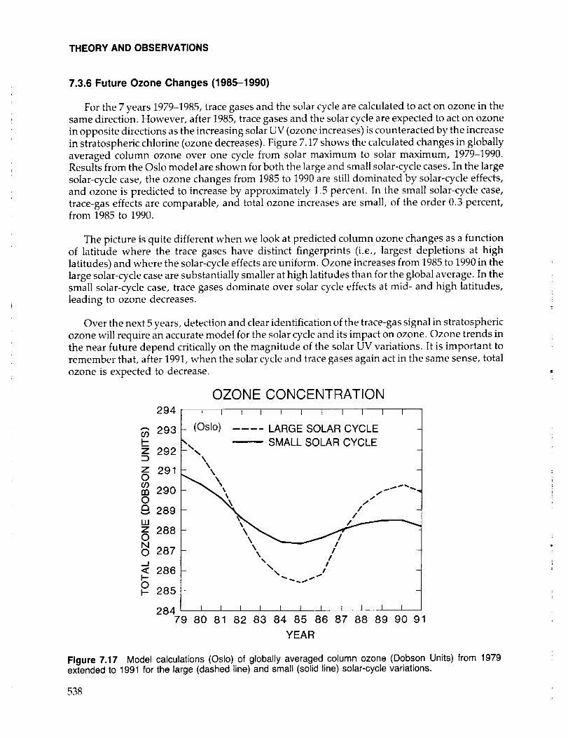
THEORY AND OBSERVATIONS

7.3.6 Future Ozone Changes (1985-1990)

For the 7 years 1979-1985, trace gases and the solar cycle are calculated to act on ozone in the

same direction. However, after 1985, trace gases and the solar cycle are expected to act on ozone

in opposite directions as the increasing solar UV (ozone increases) is counteracted by the increase

in stratospheric chlorine (ozone decreases). Figure 7.17 shows the calculated changes in globally

averaged column ozone over one cycle from solar maximum to solar maximum, 1979-t990.Results from the Oslo model are shown for both the large and small solar-cycle cases. In the large

solar-cycle case, the ozone changes from 1985 to 1990 are still dominated by solar-cycle effects,

and ozone is predicted to increase by approximately 1.5 percent. In the small solar-cycle case,

trace-gas effects are comparable, and total ozone increases are small, of the order 0.3 percent,from 1985 to 1990.

The picture is quite different when we look at predicted column ozone changes as a function

of latitude where the trace gases have distinct fingerprints (i.e., largest depletions at high

latitudes) and where the solar-cycle effects are uniform. Ozone increases from 1985 to 1990 in the

large solar-cycle case are substantially smaller at high latitudes than for the global average. In the

small solar-cycle case, trace gases dominate over solar cycle effects at mid- and high latitudes,

leading to ozone decreases.

Over the next 5 years, detection and clear identification of the trace-gas signal in stratospheric

ozone will require an accurate model for the solar cycle and its impact on ozone. Ozone trends in

the near future depend critically on the magnitude of the solar UV variations. It is important to

remember that, after 1991, when the solar cycle and trace gases again act in the same sense, total

ozone is expected to decrease.

294

292

291

290

_289

288ONO 287

< 286

O285 -

OZONE CONCENTRATION

t I 1 t I I t I I I t

_ (Oslo) .... LARGE SOLAR CYCLE

',,, SMALL SOLAR CYCLE

\\

_ "_ //

_\ /

- \ /\ /

N !¢

284 _ I I I I t I I I_ I I79 80 81 82 83 84 85 86 87 88 89 90 9

YEAR

Figure 7.17 Model calculations (Oslo) of globally averaged column ozone (Dobson Units) from 1979extended to 1991 for the large (dashed line) and small (solid line) solar-cycle variations.

538

THEORY AND OBSERVATIONS

7.3.7 How Good Are the Models?

The models participating in this study have a certain degree of realism in that they can predictabsolute concentrations of ozone, including its latitudinal, altitudinal, and seasonal variations.

This general success of the models regarding ozone does not, of course, imply that the models

can correctly describe all the remaining chemical species of the stratosphere. Nor, for that matter,

does it imply that perturbations to ozone can be predicted with great confidence.

In this study we have made several systematic comparisons among the four 2-D models.

These intercomparisons show a good qualitative, and even quantitative, agreement between the

models in most cases. Some of the disagreement can be understood from the differences inmodel structure. However, there are important differences in predictions for the lower strato-

sphere, which clearly underline the need for further comparisons both among models andbetween models and observations, especially in the lower stratosphere. The ultimate test of

predicting trends with these models would be a comparison between calculated and observedvariations on a time scale of decades, such as we have attempted here with only limited global

data.

An obvious failing of all the stratospheric models used in assessing future perturbations toozone was the Antarctic ozone hole. From intensive studies of the Antarctic ozone problem (see

Chapter 11) we have found that PSC's play a major rote in the gas-phase chemistry of the lower

stratosphere, and even have identified an important new species in the laboratory, C1202, with a

new catalytic cycle for destruction of ozone. Furthermore, we have recognized the unique

stratospheric circulation associated with the Southern Hemisphere, in particular the isolation of

the springtime Antarctic vortex. We have found unusually low levels of long-lived trace gases

(N20, CFC's) in the wintertime lower stratosphere over both poles. These recent findings haveled to substantial revisions both to the chemistry and transport of stratospheric models, but the

changes to the models will not fix all of the discrepancies with regard to observations. Most ofthese improvements have not yet been applied to the type of calculations described here,

although in the next 2 years we should expect to see assessments of future ozone change,

including the effects of heterogeneous chemistry, PSC's and precipitation, and winter polarvortices.

Future studies and assessments should attempt to improve our confidence in the strato-

spheric models by addressing the following questions:

• Which species should we measure to provide key tests of models?

• Can we design strategies to detect early changes in the ozone?

• How do we define a "good fit" between models and observations?

7.4 CONCLUSIONS

Ozone concentrations in the atmosphere vary on different time scales and for several

different causes. The models described in this chapter are designed to simulate the effect on

ozone of changes in the concentration of such trace gases as CFC, CH4, N20, and CO2. Changes

from year to year in UV radiation associated with the solar cycle are also included in the models.A third source of variability explicitly considered is the sporadic introduction of large amounts of

NO× into the stratosphere during atmospheric nuclear tests.

539

THEORY AND OBSERVATIONS

On the other hand, the models are not designed to simulate variations associated with

weekly meteorological variations, but should be able to calculate the average seasonal variation.

Thus, the effects of the pronounced QBO in the wind systems of the lower stratosphere and of

the ENSO on circulation of the tropical troposphere are not considered in the models. Another

important limitation of the models is that they do not attempt to simulate effects of volcanic

eruptions or of condensed-phase processes in general (i.e., heterogeneous chemistry and

physics). This means that the Antarctic ozone hole does not show up in any of the modelsimulations discussed here.

The performance of the models has been tested by comparing the simulations againstobservations of ozone and some other key chemical compounds. The observations exhibit

substantial variability in both space and time that is not reflected in the model simulation.

Nevertheless the average seasonal variations of the ozone concentration as a function of heightand latitude are simulated quite well. We have difficulty quantifying the uncertainty associated

with the calculations of ozone changes due to systematic changes in forcing, such as increasing

concentrations of CFC's. The ultimate test of the models in this context is a comparison between

calculated and observed variations on time scales of years to decades.

A major source of uncertainty in 2-D models is the treatment of the troposphere: its

chemistry, its zonal inhomogeneities, and the ability to predict changes in tropospheric ozone

due to trace gas changes (CH4, NOx, NMHC's, CO). Over the time period considered here,increases in tropospheric CH4, CO, and NO× are likely to have led to significant increases in

tropospheric ozone. Changes in tropospheric ozone may be large enough (-10 percent) toobscure small changes (-1 percent) in total column ozone resulting from changes in the

stratosphere.

The series of atmospheric nuclear tests during the late I950's to early 1960's represent an

interesting test case. All four models show a substantial, though different, depletion of total

ozone during the year following the large explosion in late 1962. A depletion of similar

magnitude seems to be borne out by the observations of total ozone. However, the data are

sparse and may not be representative of this period. Furthermore, the observed decrease inozone appeared to start prior to the main bomb tests. No firm conclusions can be drawn from this

simulation of the atmospheric nuclear tests.

Calculated changes in ozone due to increasing trace gas have specific patterns with latitude,

altitude, and season (i.e., fingerprints) that differ from those resulting from solar-cycle vari-

ations. The primary impact of the trace-gas scenario is due to increasing levels of stratospheric

chlorine. The fingerprint on column ozone of the trace gases for 1979-1985 shows a maximum

variation at high latitude, with larger decreases occurring during late winter (0.75-1.5) percentand smaller decreases during summer (0.25-0.5) percent. A uniform decrease of 0.3-0.5 percent

over the Tropics is estimated in the three models for which comparisons are available. The

corresponding vertical profiles show depletion peaked at 40 km of the order of 7-10 percent at

high latitudes and 3-5 percent in the Tropics.

As solar activity declines from maximum to minimum (1979 to 1985), the column ozone is

predicted to decrease almost uniformly across all latitudes and seasons. The magnitude of this

change in column ozone depends on the UV variations and ranges from about -2 percent for the

large solar-cycle case to about -0.7 percent for the small solar-cycle case. The corresponding

profiles decrease everywhere above 25 km with a broad extreme of about -3 percent near 40

km--a pattern that is less pronounced but similar to that from increases in CFC's.

54O

THEORY AND OBSERVATIONS

Can we distinguish between solar-cycle changes in ozone and those induced by increases inCFC's and CH4? The answer to this question requires the testing of all aspects of the fingerprints

of the two perturbing influences. The first approach is to look at the long-term record from theDobson network in a search for a cyclic change in column ozone that is correlated with solar

activity over the solar cycle. The statistical uncertainty of the observed amplitude is large, and thesolar cycle amplitude not well known. For this reason, the trace-gas signal cannot be clearly

separated from the record by subtracting the solar effect.

Another approach used to remove the effects of the solar cycle and short-term variations is to

average the Dobson record over two separate ll-year periods, assuming that different solar

cycles have the same integrated impact on column ozone. Wintertime Dobson data for 1976-1986

are consistently lower than those from 1965-1975. The change was most pronounced at high-

and midlatitudes (50-60°N), and about -3 percent at 60°N. This observed decrease in ozone over

the period is substantially larger than that predicted by 2-D models on the basis of the adopted

trace gas scenarios. The pattern is similar to the trace-gas fingerprint, indicating the possibilitythat the trace-gas effect is underpredicted. This is not sufficient reason, however, merely to scale

the results for the trace-gas scenario without determining the source of error, such as the

omission of certain physics and chemistry from the models.

The satellite data from TOMS/SBUV provide a more global picture of ozone, but only since

late 1978. This period, 1979-1986, is one in which both the solar cycle and trace gases are expectedto act in the same sense--that is, to reduce column ozone. The pattern of changes observed by

TOMS corroborates the evidence from the ll-year average of the Dobson data: large decreases in

ozone have occurred at high latitudes in both hemispheres in winter. To obtain a separation of

the fingerprints of trace gases and solar cycle, global satellite data must be extended through thenext solar maximum (circa 1991).

The observed changes in ozone concentration at different altitudes may also provide evi-dence of specific perturbations. The most reliable record for absolute changes in ozone profiles

over the past decade is limited to satellite instruments, SAGE-I and SAGE-II, and to the recently

analyzed Umkehr data (see Chapter 5). The difference between average ozone profiles from theSAGE instruments in 1979 and 1985 show a maximum change near 40 km of -4 + 4 percent, and

from the Umkehr observations -9 + 5 percent between 1979 and 1986. This should be compared

with a range of -6 percent to -10 percent predicted for the combined effects of increase in CFC'sand decrease in solar UV. Although the decrease appears to be dominated by trace gases, the

height profile is not sufficiently unique to make a definitive identification of fingerprints from

trace gases.

The effect of the solar cycle on ozone after its passing through its minimum during 1985 isexpected to be opposite that of the trace gases until the next solar maximum. Knowledge of the

magnitude of the solar cycle impact is essential for predicting the change in total ozone during

this period. The large solar-cycle case gives ozone changes that dominate over trace gas effects at

all latitudes through 1990. Calculations using this model for solar variability predict an increase

in globally averaged column ozone greater than 1 percent over this period. However, the small

solar-cycle model with a less pronounced solar variation in UV flux gives ozone changes that arenear zero over the next few years. Furthermore, the small solar-cycle model gives a distinct

fingerprint over the next few years in which total ozone increases at low latitudes (solar-cycle

effects dominate) and decreases at high latitudes (trace-gas effects dominate).

541

THEORY AND OBSERVATIONS

Obviously, our lack of knowledge of the magnitude of the solar-cycle variations in the UVlimits our ability to identify fingerprints in the observed ozone changes over the next few years.

Furthermore, the prediction of future ozone depletion from trace gases with the current 2-D

models is uncertain because of the lack of heterogeneous chemistry in the models used here. We

are still unsure whether the discrepancy between models and observations in the Northern

Hemisphere over the past 20 years is statistically significant and, even if it is, we are unable to say

how this error will propagate for future predictions of ozone.

542