theoretical investigation of stimulated brillouin ... · theoretical investigation of stimulated...
TRANSCRIPT

Theoretical Investigation of stimulatedBrillouin scattering in Optical Fibers and
their Applications
by
Daisy Williams
Thesis submitted to theFaculty of Graduate and Postdoctoral Studies
in partial fulfillment of the requirementsfor the Doctorate in Philosophy degree in Physics
Department of PhysicsFaculty of Science
University of Ottawa
© Daisy Williams, Ottawa, Canada, 2014

ii
To my parents

iii
Abstract
In 1920, Leon Brillouin discovered a new kind of light scattering – Brillouin scattering –
which occurs as a result of the interaction of light with a transparent material’s temporal
periodic variations in density and refractive index. Many advances have since been made in
the study of Brillouin scattering, in particular in the field of fiber optics. An in-depth
investigation of Brillouin scattering in optical fibers has been carried out in this thesis, and
the theory of stimulated Brillouin scattering (SBS) and combined Brillouin gain and loss has
been extended. Additionally, several important applications of SBS have been found and
applied to current technologies.
Several mathematical models of the pump-probe interaction undergoing SBS in the
steady-state regime have emerged in recent years. Attempts have been made to find
analytical solutions of this system of equations, however, previously obtained solutions are
numerical with analytical portions and, therefore, qualify as hybrid solutions. Though the
analytical portions provide useful information about intensity distributions along the fiber,
they fall short of describing the spectral characteristics of the Brillouin amplification and the
lack of analytical expressions for Brillouin spectra substantially limits the utility of the
hybrid solutions for applications in spectral measurement techniques. In this thesis, a highly
accurate, fully analytic solution for the pump wave and the Stokes wave in Brillouin
amplification in optical fibers is given. It is experimentally confirmed that the reported
analytic solution can account for spectral distortion and pump depletion in the parameter
space that is relevant to Brillouin fiber sensor applications. The analytic solution provides a
valid characterization of Brillouin amplification in both the low and high nonlinearity regime,
for short fiber lengths. Additionally, a 3D parametric model of Brillouin amplification is
proposed, which reflects the effects of input pump and Stokes powers on the level of pump
wave depletion in the fiber, and acts as a classification tool to describe the level of similarity
between various Brillouin amplification processes in optical fibers.
At present, there exists a multitude of electro-optic modulators (EOM), which are used to
modulate the amplitude, frequency, phase and polarization of a beam of light. Among these
iv
modulators, phase modulation provides the highest quality of transmitted signal. As such, an
improved method of phase-modulation, based on the principles of stimulated Brillouin
scattering, as well as an optical phase-modulator and optical phase network employing the
same, has been developed.
Due to its robustness, low threshold power, narrow spectrum and simplicity of operation,
stimulated Brillouin scattering (SBS) has become a favourable underlying mechanism in
fiber-based devices used for both sensing and telecommunication applications. Since
birefringence is a detrimental effect for both, it is important to devise a comprehensive
characterization of the SBS process in the presence of birefringence in an optical fiber. In this
thesis, the most general model of elliptical birefringence in an optical fiber has been
developed for a steady-state and transient stimulated Brillouin scattering (SBS) interaction,
as well as the combined Brillouin gain and loss regime. The impact of the elliptical
birefringence is to induce a Brillouin frequency shift and distort the Brillouin spectrum –
which varies with different light polarizations and pulse widths. The model investigates the
effects of birefringence and the corresponding evolution of spectral distortion effects along
the fiber, and proposes regimes that are more favourable for sensing applications related to
SBS – providing a valuable prediction tool for distributed sensing applications.
In recent years, photonic computing has received considerable attention due to its numerous
applications, such as high-speed optical signal processing, which would yield much faster
computing times and higher bandwidths. For this reason, optical logic has been the focus of
many research efforts and several schemes to improve conventional logic gates have been
proposed. In view of this, a combined Brillouin gain and loss process has been proposed in a
polarization maintaining optical fiber to realize all-Optical NAND/NOT/AND/OR logic
gates in the frequency domain. A model describing the interaction of a Stokes, anti-Stokes
and a pump wave, and two acoustic waves inside a fiber, ranging in length from
350m-2300m, was used to theoretically model the gates. Through the optimization of the
pump depletion and gain saturation in the combined gain and loss process, switching
contrasts of 20-83% have been simulated for different configurations.

v
Statement of Originality
This work contains no material which has been accepted for the award of any other degree or
diploma in an University or other tertiary institution and, to the best of my knowledge and
belief, contains no material previously published or written by another person, except where
due reference has been made in the text.
I give consent to this copy of my thesis, when deposited in the University Library, being
available for loan and photocopying.
SIGNED: ____________________________
DATED: _____________________________
Supervisors: Dr. Xiaoyi Bao and Dr. Liang Chen

vi
Acknowledgments
It is my pleasure to take this opportunity to thank all the people who have helped
me over the past few years.
First of all, I would like to thank my supervisors Dr. Xiaoyi Bao and Dr. Liang Chen, who
invited me to join their group as a graduate student and gave me the chance to do research on
stimulated Brillouin scattering (SBS) in optical fibers. I am grateful for the opportunity to
have worked in their Fiber Optics Group at the University of Ottawa, in an environment
which supported and motivated me to achieve my goals. I would like to thank Dr. Xiaoyi Bao
and Dr. Liang Chen for the interest they showed in my progress and for the guidance they
gave me. Their diligence and persistence in both research and mentorship is deeply
appreciated. Their critical and thoughtful approach to problems was always instructive.
I must give many thanks to my colleagues in Fiber Optics Group at University of Ottawa.
Their comments and suggestions have greatly benefited me. Special thanks to Bhavaye
Saxena for interesting discussions and Dr. Dapeng Zhou for helping with my experimental
setup. Their kind help and valuable suggestions went a long way in furthering my research
goals.
I am deeply indebted to my parents. Their enduring love and support gave me the strength to
overcome the challenges of being a Ph.D. student. To them, I dedicate this thesis.
Daisy Williams

vii
Table of ContentsAbstract......................................................................................................................... iiiAcknowledgments........................................................................................................ viList of Figures............................................................................................................... xList of Tables................................................................................................................. xivList of Acronyms.......................................................................................................... xv
Chapter 1. Introduction............................................................................................... 11.1 Overview................................................................................................ 11.2 3D parametric model............................................................................ 21.3 SBS optical phase modulator............................................................... 31.4 Polarization effects in SBS................................................................... 41.5 Photonic Logic....................................................................................... 61.6 Thesis contributions.............................................................................. 81.7 Thesis outline......................................................................................... 10
Chapter 2. Physics of Brillouin Scattering................................................................. 122.1 Introduction........................................................................................... 122.2 Light Scattering .................................................................................... 122.3 Spontaneous Brillouin Scattering........................................................ 142.4 Stimulated Brillouin Scattering........................................................... 18
2.4.1 SBS Generator......................................................................... 182.4.2 SBS Amplifier........................................................................... 192.4.3 Electrostriction......................................................................... 192.4.4 SBS Coupled wave equations and
configuration........................................................................... 202.4.5 Combined Brillouin gain and loss coupled
wave equations and configuration......................................... 232.5 Polarization and birefringence............................................................ 25
2.5.1 Polarization states.................................................................... 252.5.2 Polarization Ellipse.................................................................. 262.5.3 Poincaré Sphere....................................................................... 282.5.4 Birefringence............................................................................ 30
2.6 Summary................................................................................................ 31
Chapter 3. 3D parametric model................................................................................ 323.1. Introduction.......................................................................................... 323.2 Model...................................................................................................... 333.3 Solution.................................................................................................. 363.4 Analytic Solutions.................................................................................. 39
3.4.1 Linear approximation............................................................. 403.4.2 Quadratic approximation....................................................... 41
3.5 Relative error......................................................................................... 413.5.1 Linear Approximation............................................................. 423.5.2 Quadratic Approximation....................................................... 43

viii
3.6 3D parametric model............................................................................ 443.7 3D parametric model: Similar and Dis-similar Processes.................. 453.8 Applications in Fiber Sensing.............................................................. 483.9 Spectral Characteristics....................................................................... 49
3.9.1 Analytical expressions............................................................. 493.9.2 Transition to a Lorentzian Spectra (Curvature)................... 52
3.10 Experiment.......................................................................................... 553.10.1 Experimental Setup............................................................... 553.10.2 Experimental Results............................................................ 56
3.11 Summary.............................................................................................. 57
Chapter 4. SBS Optical Phase Modulator and Network.......................................... 584.1 Introduction........................................................................................... 584.2 Theory.................................................................................................... 584.3 Proposed Experimental Setup.............................................................. 634.4 Optical phase modulator construction................................................ 674.4 Optical network transmission lines with phase-modulated carriers 684.5 Summary................................................................................................ 72
Chapter 5. Polarization Effects in SBS...................................................................... 735.1 Introduction........................................................................................... 735.2 Model...................................................................................................... 745.3. Results and Discussion......................................................................... 79
5.3.1 Spectral Shift............................................................................ 795.3.2 Spectral Distortion................................................................... 82
A. Linear Polarization (LP).............................................. 82B. Elliptical Polarization for steady-state interaction.... 86
5.4 Summary................................................................................................ 90
Chapter 6. Polarization Effects in combined Brillouin gain and loss...................... 916.1 Introduction........................................................................................... 916.2 Model...................................................................................................... 916.3 Results and Discussion.......................................................................... 98
6.3.1. Gain dominant regime............................................................ 986.3.2 Competing Gain and Loss regime.......................................... 102
6.4 Summary................................................................................................ 105
Chapter 7. Applications of SBS: Photonic Logic....................................................... 1067.1 Introduction........................................................................................... 1067.2 Model...................................................................................................... 1067.3 Results and Discussion.......................................................................... 1107.4 NAND gate............................................................................................. 110
7.4.1 Configuration I........................................................................ 1107.4.2 Configuration II....................................................................... 1117.4.3 Configuration III..................................................................... 112
7.5 NOT gate................................................................................................ 1147.5.1 Configuration IV...................................................................... 114

ix
7.5.2 Configuration V....................................................................... 1157.6 AND gate................................................................................................ 115
7.6.1 Configuration VI...................................................................... 1157.6.2 Configuration VII.................................................................... 1177.6.3 Configuration VIII................................................................... 118
7.7 OR gate.................................................................................................. 1197.7.1 Configuration IX...................................................................... 1197.7.2 Configuration X....................................................................... 1207.7.3 Configuration XI...................................................................... 122
7.8 General method of logic gate construction......................................... 1237.8.1 Configuration V: NOT gate..................................................... 1237.8.2 Configuration IV: NOT gate................................................... 1257.8.3 Configurations I and II: NAND gates.................................... 1267.8.4 Configuration III: NAND gate............................................... 1277.8.5 3D parametric model applications in photonic logic............ 129
7.9 Proposed Experimental Configurations.............................................. 1307.9.1 Configurations I-V................................................................... 1307.9.2 Configurations VI.................................................................... 1327.9.3 Configurations VII................................................................... 1347.9.4 Configurations IX.................................................................... 1357.9.5 Configurations X...................................................................... 1377.9.6 Configurations XI.................................................................... 138
7.10 Bit rate.................................................................................................. 1407.11 Summary.............................................................................................. 140
Chapter 8. Conclusion................................................................................................. 1418.1 Thesis Outcomes.................................................................................... 1418.2 Future Work.......................................................................................... 142
Bibliography................................................................................................................. 144Appendix....................................................................................................................... 153
A. Derivation of the system of equations (5.1)-(5.4)................................. 153B. Fourth Order Runge-Kutta Method of Solution................................. 157
Curriculum Vitae......................................................................................................... 159

x
List of FiguresFigure 2.1: Schematic of the observed scattered light intensity [1]. 13Figure 2.2: Stokes Brillouin scattering [1]. (a) Relative orientations of the
wavevectors k1 and k2, (b) k1, k2 and q relationship, Schematic ofSBS interaction. 16
Figure 2.3: Anti-Stokes Brillouin scattering [1]. (a) Relative orientations of thewavevectors k1 and k3, (b) k1, k3 and q relationship, Schematic ofSBS interaction. 17
Figure 2.4: SBS generator [1]. 19Figure 2.5: SBS amplifier [1]. 19Figure 2.6: Schematic arrangement of SBS in a fiber of length L.
Pump and probe configuration: A1(z) – Pump wave, A2(z) – probewave (incident pulse). 21
Figure 2.7: Schematic distribution of the pump and probe intensities during SBS[1]. 23
Figure 2.8: Schematic arrangement of SBS in a PMF of length L.PW and pulse configuration: A1 – pump wave, A2 – Stokes wave, A3
– anti-Stokes wave. 24Figure 2.9: Different polarization states, figure taken from Wikipedia. 25Figure 2.10: Polarization Ellipse. 27Figure 2.11: Poincaré Sphere. 28Figure 3.1: Relative error of Y1(0): Linear Approximation of 3D parametric
model of output PW. L=1000m, 0<Ppump<10mW , 0<PStokes<40mW. 42Figure 3.2: Relative error of Y1(0): Quadratic Approximation of 3D parametric
model of output PW. L=1000m, 0<Ppump<10mW , 0<PStokes<40mW. 43Figure 3.3: Linear Approximation of Y1(0): 3D parametric model of output PW.
Dimensionless output intensity of the PW versus dimensionlessparameters β1 and β3. γe=0.902, v=5616 m/s, n=1.48, λ=1.319μm,ρ0=2.21 g/cm3, ΓB = 0.1 GHz, L=1000m, 0<Ppump<10mW ,0<PStokes<40mW. 44
Figure 3.4: Linear Approximation of Y2(ℓ): 3D parametric model of output SW.Dimensionless output intensity of the SW versus dimensionlessparameters β1 and β3. γe=0.902, v=5616 m/s, n=1.48, λ=1.319μm,ρ0=2.21 g/cm3, ΓB = 0.1 GHz, L=1000m, 0<Ppump<10mW,0<PStokes<40mW. 45
Figure 3.5: Linear Approximation of Y1(0): 3D parametric model of output PW.Dimensionless output intensity of the PW versus dimensionlessparameters β1 and β3. γe=0.902, v=5616 m/s, n=1.48, λ=1.319μm,ρ0=2.21 g/cm3, ΓB = 0.1 GHz, L=1000m, 0<Ppump<10mW ,0<PStokes<40mW. 47
Figure 3.6: Analytical results, normalized intensity units of the SW. PSW (mW) = 0.01; 1.8; 6.6; 12.1; 17.1; + 22.4; ⁕ 27.2; --- 31.8; 36.3; n=1.48, γe=0.902, λ=1319nm, ρ0=2.21 g/cm3, v=5616 m/s,L=1000 m, ΓB=0.1 GHz, PPW = 1.0 mW. 50

xi
Figure 3.7: Pump depletion as a function of probe spectral distortion. PSW (mW)= 0.01; 1.8; 6.6; 12.1; 17.1; + 22.4; ⁕ 27.2; 31.8; ♦36.3; n=1.48, γe=0.902, λ=1319nm, ρ0=2.21 g/cm3, v=5616 m/s,L=1000 m, ΓB=0.1 GHz, PPW = 1.0 mW. 51
Figure 3.8: Shaded area depicts range of β1 and β3 values which yield curvatureswithin 20% of the Lorentz Curvature for both PW and SW spectra. 54
Figure 3.9: Experimental setup. 55Figure 3.10: Experimental results, normalized intensity units of the SW. PSW
(mW) = 0.01; 1.8; 6.6; 12.1; 17.1; + 22.4; ⁕ 27.2; ---31.8; 36.3; n=1.48, γe=0.902, λ=1319nm, ρ0=2.21 g/cm3, v=5616m/s, L=1000m, ΓB=0.1 GHz, PPW = 1.0 mW. 56
Figure 4.1: Form factor as a function of ξ1. 61Figure 4.2: Gain factor as a function of ξ1. 62Figure 4.3: Experimental setup. 63Figure 4.4: Optical phase modulator construction. 67Figure 4.5: Optical network construction. 69Figure 5.1: Schematic arrangement of SBS in an optical fiber of length L. E1x –
Pump wave, E1y – Pump wave, E2x – Stokes wave, E2y – Stokeswave. 74
Figure 5.2: (a) Output pump spectrum, (b) output Stokes spectrum.Birefringence Δn: *10-4; 10-5; 10-6; LHP(1,0,0); L=1000m.P1x0 = 0.5 mW, P1y0 = 0.5 mW, P2x0 = 0.5 mW, P2y0 = 0.5 mW. 80
Figure 5.3: Brillouin shift dependence on beat length, L=1000m, LHP (1,0,0).(a) P1x0 = 0.9 mW, P1y0 = 0.1 mW, P2x0 = 0.9 mW, P2y0 = 0.1 mW.(b) P1x0 = 0.5 mW, P1y0 = 0.5 mW, P2x0 = 0.5 mW, P2y0 = 0.5 mW. 81
Figure 5.4: Left: output pump spectrum; Right: output Stokes spectrum. (a)-(b)steady-state; (c)-(d) 240ns pulse; (e)-(f) 79ns pulse; BirefringenceΔn=10-4; L=1 km. : P1x0 = 10.0 mW, P1y0 = 1.0 mW, P2x0 = 10.0mW, P2y0 = 1.0 mW; LHP (1,0,0); : P1x0 = 10.9 mW, P1y0 = 0.1mW, P2x0 = 10.9 mW, P2y0 = 0.1 mW; LHP (1,0,0); : P1x0 = 10.0mW, P1y0 = 1.0 mW, P2x0 = 10.0 mW, P2y0 = 1.0 mW; no pol (0,0,0).
82-83
Figure 5.5: (a) x-comp. of output Stokes spectrum; (b) y-comp. of output Stokesspectrum. Birefringence Δn = * 10-4 ; 10-5; 10-6; Random4(0.1,0.9,0.42), L=1000m. P1x0 = 10.0 mW, P1y0 = 1.0 mW, P2x0 = 10.0mW, P2y0 = 1.0 mW. 87
Figure 5.6: (a) Output pump spectrum, (b) Output Stokes spectrum.Birefringence Δn: 10-6 Random1 (0.6, 0.25, 0.76); 10-6
Random2 (0.3, 0.7, 0.65); L=1000m. 10-6 Random3 (0.58, 0.58,0.58); * 10-6 Random4 (0.1, 0.9,0.42); 10-10 no pol (0,0,0); P1x0 =1.0 mW, P1y0 = 1.0 mW, P2x0 = 1.0 mW, P2y0 = 80.0 mW. 88
Figure 5.7: (a) Output pump spectrum, (b) output Stokes spectrum.Birefringence Δn: 10-6 Random1 (0.6, 0.25, 0.76); 10-6
Random2 (0.3, 0.7, 0.65); L=1000m. 10-6 Random3 (0.58, 0.58,0.58); * 10-6 Random4 (0.1, 0.9,0.42); 10-10 no pol (0,0,0); P1x0 =10.0 mW, P1y0 = 1.0 mW, P2x0 = 60.0 mW, P2y0 = 1.0 mW. 89
Figure 6.1: Schematic arrangement of SBS in an optical fiber of length L. E1x –

xii
Pump wave, E1y – Pump wave, E2x – Stokes wave, E2y – Stokeswave, E3x – anti-Stokes wave, E3y – anti-Stokes wave. 92
Figure 6.2: Output pump spectra. S=(0.1, 0.9, 0.42). L=45m. P1x=P1y=1mW. (a)P2x=P2y=P3x=P3y=0.1mW; (b) P2x=P2y=P3x=P3y=0.2mW; (c)P2x=P2y=P3x=P3y=0.3mW; (d) P2x=P2y=P3x=P3y=0.4mW; (e)P2x=P2y=P3x=P3y=0.5mW; (f) P2x=P2y=P3x=P3y=0.6mW.
:Δn =10-4; : Δn =10-5; : Δn =10-6; :Δn =10-10
S=(0, 0, 0). 99Figure 6.3: (A) ΔυB dependence on Δn; (B) Ratio dependence on Δn. L=45m,
S=(0.1, 0.9, 0.42). (a) P2x=P2y=P3x=P3y=0.1mW; (b)P2x=P2y=P3x=P3y=0.2mW; (c) P2x=P2y=P3x=P3y=0.3mW; (d)P2x=P2y=P3x=P3y=0.4mW; (e) P2x=P2y=P3x=P3y=0.5mW; (f)P2x=P2y=P3x=P3y=0.6mW. 100
Figure 6.4: Output pump spectra. S=(0.1, 0.9, 0.42). L=45m. P1x=P1y=1mW.(a) P2x=P2y=P3x=P3y=0.7mW; (b) P2x=P2y=P3x=P3y=0.8mW; (c)P2x=P2y=P3x=P3y=0.9mW; : Δn =10-4; :Δn =10-5;
:Δn =10-6; :Δn =10-10 S=(0, 0, 0). 102Figure 6.5: (A) ΔυB dependence on Δn; (B)-(C) Ratio dependence on Δn. L=45m,
S=(0.1, 0.9, 0.42). (a) P2x=P2y=P3x=P3y=0.7mW; (b)P2x=P2y=P3x=P3y=0.8mW; (c) P2x=P2y=P3x=P3y=0.9mW. 103
Figure 7.1: ASW power distribution inside the optical fiber. (a) Gain and Lossregime: P20=10mW; (b) Gain or Loss regime: P20=0mW. n=1.48,γe=0.902, λ=1550nm, ρ0=2.21 g/cm3, v=5616 m/s, ΓB=0.1 GHz,α=0.2 dB/km, L=350m, P10=10mW, P30=10mW. 110
Figure 7.2: NAND gate switching contrast plots. (a) Configuration I: Lowthreshold: 54.7%, High threshold: 74.8%, Tolerance: 20.6%. (b)Configuration II: Low threshold: 35.8%, High threshold: 87.8%,Tolerance: 52.7%. (c) Configuration III: Low threshold: 5.9%, Highthreshold: 87.7%, Tolerance: 82.8%. 111
Figure 7.3: Output ASW power spectra. (a) ‘0 0’ input, (b) ‘0 1’ input, (c) ‘1 0’input, (d) ‘1 1’ input.
112-113
Figure 7.4: NOT gate switching contrast plots. (a) Configuration IV: Lowthreshold: 38.9%, High threshold: 91.1%, Tolerance: 52.9%.(b)Configuration V: Low threshold: 13.3%, High threshold: 90.0%,Tolerance: 77.6%. 114
Figure 7.5: Schematic of Configuration VI: AND gate. 116Figure 7.6: AND gate switching contrast plots. Configuration VI: Low
threshold: 40.2%, High threshold: 83.1%, Tolerance: 42.3%.Configuration VII: Low threshold: 16.1%, High threshold: 77.1%,Tolerance: 61.8%. 116
Figure 7.7: Schematic of Configuration VII: AND gate. 117Figure 7.8: Schematic of Configuration IX: OR gate. 119Figure 7.9: OR gate switching contrast plot. Low threshold: 6.8%, High
threshold: 88.9%, Tolerance: 83.0%. 120Figure 7.10: (a) Schematic of configuration X: OR gate, (b) OR gate switching
contrast plot, Low threshold: 7.04%, High threshold: 90.6%,

xiii
Tolerance: 83.6%. 121Figure 7.11: (a) Schematic of configuration XI: OR gate, (b) OR gate switching
contrast plot, Low threshold: 7.22%, High threshold: 89.6%,Tolerance: 82.4%. 122
Figure 7.12: Flow chart for NOT gate of configuration V. 124Figure 7.13: Flow chart for NOT gate of configuration IV. 125Figure 7.14: Flow chart for NAND gate of configurations I and II. 126Figure 7.15: Flow chart for NAND gate of configuration III. 128Figure 7.16: NOT experimental setup for test of NAND/NOT gates.
(a) Configurations I-IV, (b) Configuration V. DFB: DistributedFeedback, RF: radio frequency, C: circulator, CC: fiber coupler,FUT: fiber under test, I: isolator, EOM: Electro-Optic Modulator,FBG: Fiber Bragg Grating, PC: polarization controller, EDFA:Erbium-doped fiber amplifier, DAQ: Data Acquisition. 131
Figure 7.17: Configuration VI: AND gate. DFB: Distributed Feedback, RF: radiofrequency, C: circulator, CC: fiber coupler, RR: ring resonator, FUT:fiber under test, I: isolator, EOM: Electro-Optic Modulator, FBG:Fiber Bragg Grating, PC: polarization controller, EDFA:Erbium-doped fiber amplifier, DAQ: Data Acquisition. 133
Figure 7.18: Configuration VII: AND gate. DFB: Distributed Feedback, RF: radiofrequency, C: circulator, CC: fiber coupler, RR: ring resonator, FUT:fiber under test, I: isolator, EOM: Electro-Optic Modulator, FBG:Fiber Bragg Grating, PC: polarization controller, EDFA:Erbium-doped fiber amplifier, DAQ: Data Acquisition. 134
Figure 7.19: Configuration IX: OR gate. DFB: Distributed Feedback, RF: radiofrequency, C: circulator, CC: fiber coupler, RR: ring resonator, FUT:fiber under test, I: isolator, EOM: Electro-Optic Modulator, FBG:Fiber Bragg Grating, PC: polarization controller, EDFA:Erbium-doped fiber amplifier, DAQ: Data Acquisition. 136
Figure 7.20: Configuration XI: OR gate. DFB: Distributed Feedback, RF: radiofrequency, C: circulator, CC: fiber coupler, RR: ring resonator, FUT:fiber under test, I: isolator, EOM: Electro-Optic Modulator, FBG:Fiber Bragg Grating, PC: polarization controller, EDFA:Erbium-doped fiber amplifier, DAQ: Data Acquisition. 139

xiv
List of Tables
Table 4.1: Simulation results for the experimental setup....................................... 66Table 7.1: Simulation Parameters.......................................................................... 109

xv
List of AcronymsDFB: Distributed FeedbackRF: Radio FrequencyC: circulatorCC: Fiber CouplerRR: Ring ResonatorFUT: Fiber Under TestI: IsolatorEOM: Electro-Optic ModulatorFBG: Fiber Bragg GratingPC: Polarization ControllerEDFA: Erbium-doped fiber amplifierDAQ: Data AcquisitioneVOA: Electronic Variable Optical AttenuatorAOM: Acoustic-Optic ModulatorBGS: Brillouin gain spectrumBLS: Brillouin loss spectrumBOFDA: Brillouin Optical Frequency Domain AnalysisBOTDA: Brillouin Optical Time Domain AnalysisBOTDR: Brillouin Optical Time Domain ReflectometerCW: Continuous wavePW: Pump waveSW: Stokes waveASW: Anti-Stokes waveAW: Acoustic waveDBS: Distributed Feedback laserEM ElectromagneticEOM: Electro-Optic ModulatorFWHM: Full width at Half MaximumODPA: Optical Differential Parametric AmplificationOSA: Optical Spectrum AnalyzerOTDA: Optical Time Domain AnalysisOTDR: Optical Time Domain ReflectometerPM: Polarization MaintainingPMF: Polarization Maintaining FiberSBS: Stimulated Brillouin ScatteringSNR: Signal-to-Noise RatioSOP: State of PolarizationPDL: Polarization Dependent LossPMD: Polarization Mode DispersionHOM: High-Order ModeLHS: Left-hand sideRHS: Right-hand sideSMF: Single-mode fiberAM: Amplitude-Modulated

xvi
UPA: Undepleted Pump ApproximationRK4 Fourth Order Runge-KuttaRK6 Sixth Order Runge-KuttaLP: Linear Polarization or Linearly PolarizedLHP: Linearly Horizontally PolarizedLVP: Linearly Vertically PolarizedL+45P: Linear +45° PolarizedL-45P: Linear -45° PolarizedLCP: Left Circularly PolarizedRCP: Right Circularly PolarizedBOCDA: Brillouin optical correlation-domain analysisMZI: Mach-Zehnder InterferometerSOA: Semiconductor Optical AmplifiersHNLF: Highly Nonlinear Fiber
1
Chapter 1
Introduction
1.1 Overview
In 1920, a new kind of light scattering was discovered by Leon Brillouin – Brillouin
scattering – which occurs as a result of the interaction of light with a transparent material’s
temporal periodic variations in density and refractive index. The result of this interaction
between the light wave and the material is a change in the momentum of the light wave
(frequency and energy) along preferential angles, similar to the diffraction off a moving
grating. Many advances have since been made in the study of Brillouin scattering, in
particular in the field of fiber sensing and fiber optics.
This thesis focuses on the investigation and applications of Brillouin scattering in optical
fibers. The current chapter introduces the background, motivation, and contributions of the
research work. Section 1.2 describes previously obtained solutions for SBS, which are
numerical with analytical portions, and illustrates the motivation of developing a fully
analytical solution of the Brillouin amplification problem valid for an arbitrary high
depletion. Section 1.3 provides an overview of existing optical phase modulation devices and
techniques and their limitations, and presents an optical phase modulation technique based
on the principles of SBS, which would mitigate the disadvantages of existing technologies.
Section 1.4 focuses on the investigation of a more accurate model of the
polarization-dependent SBS interaction, including the possibility of elliptical birefringence,
and its effect on the SBS process. Section 1.5 presents a polarization-independent technique
to accurately realize all-optical logic gates based on the principles of combined Brillouin
gain and loss in an optical fiber. Section 1.6 explains the thesis contributions, and section 1.7
provides the thesis outline.

2
1.2 3D parametric model
Since the discovery of stimulated Brillouin scattering (SBS) in optical fibers, several
mathematical models of the pump-probe interaction undergoing SBS in the steady-state
regime have emerged, which are valid for pulse lengths greater than the phonon relaxation
time [1]. The two-wave interaction is modeled by a system of ordinary differential equations,
which in most cases [2, 3] has solved numerically. However, numerical solutions not lend
themselves easily to the high pump wave depletion-related optimization procedures that are
essential for applications in strain and temperature sensing. For example, distributed sensing,
using an EDFA (Erbium Doped Fiber Amplifier) and distributed Raman amplifiers [4, 5, 6]
has the potential to lead to high pump depletion and would require an appropriately accurate
solution.
Several attempts have been made to find analytical solutions of this system of equations. The
most common is the undepleted pump approximation (UPA), employed in [7], which
imposes the assumption that the pump wave depletion, due to energy transfer between the
pump and probe waves, is negligible. The lack of pump wave depletion is a coarse
approximation which does not reflect the challenges of fiber sensing techniques.
In [8, 9] an analytical solution for a lossless fiber has been attempted without putting limits
on the level of depletion. However, this attempt has been only partially successful – the
system of ordinary differential equations has been reduced to a transcendental equation,
which still has to be solved numerically.
An interesting technique has been used in [1] to find the analytical solutions for a lossy fiber,
placing no limits on the level of depletion in the fiber. The system of ordinary differential
equations has been reduced to a transcendental equation involving an integral, which,
unfortunately, could only be evaluated numerically. As a result, neither intensity distribution
along the fiber, nor Brillouin spectra could be expressed analytically. A variation of the
perturbation technique has been used in [10] with the intention of obtaining an analytical
solution for a lossy fiber. However, a solution in the zero-approximation with respect to the

3
attenuation constant has been taken from [9], which, as described above, requires the
numerical solutions of a transcendental equation. Contrary to the claim in [10], only a hybrid
solution has been obtained, which extends the solution in [6] to a lossy fiber, but otherwise
has similar limitations.
Therefore, there is still an unsatisfied need for a fully analytical solution of the Brillouin
amplification problem valid for an arbitrary high depletion, as well as a model which would
characterize the Brillouin amplification process and help mitigate the detrimental effects of
spectral depletion.
1.3 SBS optical phase modulator
At present, there exists a multitude of electro-optic modulators (EOM), which are used to
modulate the amplitude, frequency, phase and polarization of a beam of light [11, 12, 13, 14].
Among these modulators, phase modulation provides the highest quality of transmitted signal
– though at the expense of a widened spectrum. In view of the benefits, optical phase
modulation has various applications in the field of optical networks and data transmission.
The most common phase modulator uses a Lithium Niobate crystal (LiNbO3) [15, 16, 17],
which has an index of refraction that depends linearly on the applied electric field, and a
phase linearly dependent on the index of refraction. As the electric field changes, the
resulting phase is modulated. The achievable variation of the refractive index in Lithium
Niobate is relatively small, requiring either large voltages or long electrode lengths to obtain
sufficient phase modulation. Such modulators may also perform the task of amplitude
modulation.
ThorLabsTM, for example, produces Lithium Niobate phase modulators made of Titanium
Indiffused Z-Cut LiNbO3, which are especially designed to be integrated into transponders.
The Lithium Niobate component is required for all-optical frequency shifting, and
applications such as sensing and data encryption. These phase modulators are designed to

4
operate in the 1550 nm range.
JenoptikTM produces integrated optical phase modulators, which employ a combination of
Magnesium oxide (MgO) and Lithium niobate (LiNbO3) crystals to realize phase modulation
in the GHz range. An advantage with JenoptikTM phase modulators is that a relatively low
modulation voltage is required to achieve the desired phase modulation, thus being suitable
for wavelengths in the visible and infrared spectral range.
Other methods of optical phase modulation have also been employed. For example, optical
phase modulation has been achieved in a traveling wave semiconductor laser amplifier [18].
In this work, the optically controlled phase modulation is independent of the signal
wavelength.
In spite of advances made in the area of optical phase modulation, there is still a need in the
industry for developing alternative methods of optical phase modulation and further
improvements to optical networks.
1.4 Polarization effects in SBS
In recent years, due to its robustness, low threshold power, and simplicity of operation,
stimulated Brillouin scattering (SBS) has become a favourable underlying mechanism in
fiber-base devices used for both sensing and telecommunication applications [4, 19, 20, 21].
Since birefringence is a detrimental effect for both, it is important to devise a comprehensive
characterization of the SBS process in the presence of birefringence in an optical fiber, so
that a prediction of the Brillouin frequency shift and birefringence variation over different
sensing lengths can be made. All previous theoretical works [19, 22, 23, 24, 25, 26, 27] are
related to the Brillouin gain variation due to the state of polarization (SOP) change. Although
the effects of fiber birefringence on Brillouin frequency shift and linewidth have been studied
experimentally [28], no report has been made regarding the Brillouin frequency shift
associated with the SOP and birefringence change in relation to the fiber position.
5
A quantitative study of the fiber birefringence versus frequency shift is essential in finding
the maximum impact of the fiber birefringence on the measurement precision of temperature
and strain, for distributed Brillouin optical time domain analysis (BOTDA) or Brillouin
optical time domain reflectometry (BOTDR) sensors, since it will be helpful in designing the
best suitable fiber for BOTDA or BOTDR applications as well as optimizing system design.
Early works which investigated the polarization effects on SBS in optical fibers [22, 23, 24,
25] showed that the Stokes gain is strongly dependent on polarization effects, and in [29],
this theoretical work was experimentally confirmed. [26] examines the applications of optical
birefringence in SBS sensing for strain and temperature measurements, while [19] devises a
technique to overcome the sensitivity of pulse delay to polarization perturbations, enhancing
SBS slow light delay. In [27], a vector formalism was used to characterize the effects of
birefringence on the SBS interaction. One such effect was signal broadening as a result of
polarization effects. However, only linearly polarized (LP) pump and signal waves were
investigated in [26, 27]. Additionally, [27] assumed an undepleted pump regime, which has
applications only for short fiber lengths, while the BOTDA and BOTDR often operate on
long fiber distances; the convolution of the birefringence and depletion would induce much
larger distortion on the Brillouin spectrum, and hence lower the temperature and strain
resolution. Thus the undepleted and linear polarized models are not adequate to address real
problems.
The above mentioned works [23, 24, 25, 27, 29], however, treat a steady-state SBS system
where both the pump and Stokes waves are continuous. Additionally, none of these
references investigated the effect of birefringence and polarization on the spectral distortion
– namely Brillouin frequency shift of pulses undergoing SBS. In [19], though pulse length
was taken into account, Brillouin spectrum distortion was not. More importantly, the impact
of the nonlinear effect under different pump powers convoluted with the fiber birefringence
and its impact on the Brillouin spectrum shape and peak shift have not yet been examined.
An extension of [27] was published in the work [30], whereby signal pulses were taken into
consideration and pulse distortion was observed. However, this work still did not take into
consideration the most general case of birefringence, which is elliptical birefringence. Finally,

6
none of the aforementioned works investigated the effects of polarization and birefringence
in the combined Brillouin gain and loss regime in an optical fiber.
The authors feel that it was important to investigate a more accurate model of the
polarization-dependent SBS interaction – including elliptical birefringence. Besides being
able to accommodate the most general case of elliptical birefringence, the effects of
polarization mode dispersion (PMD), polarization dependent loss (PDL), phonon resonance
structures, pulse length, as well as the overall attenuation of the fiber must be taken into
account. Finally, since spectral distortion is detrimental for fiber sensing and
telecommunications, an in depth investigation into the effects of birefringence and
polarization on the SBS process, and methods of minimizing these effects have been
investigated.
1.5 Photonic Logic
In recent years, photonic computing has received considerable attention due to its numerous
applications, such as high-speed optical signal processing, which would yield much faster
computing times and higher bandwidths. For this reason, optical logic has been the focus of
many research efforts, and several schemes to improve conventional logic gates have been
proposed. In [31, 32, 33], optically programmable and reversible Boolean logic units are
proposed, consisting of a circuit which is designed by the implementation of a 2 x 2
optoelectronic switch [34]. The drawback of this scheme is that the switching speed of the 2
x 2 switching element is about 106 times slower compared to, for example, a semiconductor
optical amplifier (SOA) based interferometric switch. In view of the speed limitations
inherent in electronic circuits, all-optical data processing devices have become the focus of
many research efforts, especially in optical fibers, as these devices provide compatibility to
fiber links with low connection loss and easy implementation. One category of such devices
is the all-optical logic gate, which is projected to be a main component in future integrated
photonic circuits.

7
Some established techniques for achieving functional all-optical logic gates include the use
of integrated optical and waveguide structure Mach-Zehnder interferometers (MZIs) [35, 36,
37] that are often limited by back-reflections of the optical signal, which are minimized by
extending the cladding and substrate layers; the use of nonlinear optical processes in
semiconductor optical amplifiers (SOA), such as four-wave mixing [38] and cross-gain
modulation [39, 40, 41]; and the use of a combination thereof – integrated Mach-Zehnder
interferometers based on SOA [42, 43, 44, 45]. SOA-based techniques are often limited by
the carrier’s recovery time which in turn slows down the operation of the device. In addition,
these techniques often require the use of multiple SOAs to achieve functional all-optical
logic gates, and fall victim to additional noise such as spontaneous emission noise [46, 47],
time dependent modulation due to time jitter, and birefringence induced signal distortion.
Additionally, there exist logic gates proposed by terahertz optical asymmetric demultiplexer
(TOAD) based switches [48, 49, 50, 51]. The TOAD consists of a loop mirror and a
nonlinear element, usually an SOA, which is positioned asymmetrically in the fiber loop. In
addition to the limitations of the SOA mentioned above, the TOAD scheme suffers from a
walk-off problem due to dispersion, intensity losses due to beam splitter, optical circulators,
etc. In addition, if there is an attempt to remedy the aforementioned finite propagation time
of the pulse across the SOA by decreasing the offset length, the decrease in effective SOA
length causes a reduction in contrast ratio of the TOAD switching mechanism, which hinders
the functionality of the logic gate.
Techniques, based on the design of simple passive optical components, also exist. These
techniques include optical logic parallel processors [52] and the multi-output
polarization-encoded optical shadow-casting scheme [53]. Both schemes are based on the
polarization of light, whereby the switching mechanism consists of the polarization switching
of output light. Drawbacks of such schemes include polarization instability, inherent in any
polarization-dependent device, and detrimental diffraction effects.
Other such techniques also exist, such as using a Kerr nonlinear prism to realize
binary-to-gray-to-binary code conversion, whereby the switching mechanism is the deviation

8
of light due to nonlinear refraction [54]. However, to function correctly, such a scheme
requires several such prisms and mirrors to be aligned in series, the configuration of which is
both bulky and requires extensive calibration. In addition, very large intensities are required
for the function of the proposed setup.
Fiber nonlinearity-based techniques provide comparable functionality, without the limitations
mentioned above. Among fiber nonlinearity-based logic gates, one of the techniques includes
using the Kerr effect in highly nonlinear fibers (HNLF) to induce birefringence, thereby
rotating the polarization state of an output light wave [55, 56], which represents the optical
gate operation with an ultimate speed limitation above 100 Gb/s. However, one limitation of
this technique is that long fiber lengths introduce polarization instabilities in conventional
single mode fibers. A relatively short fiber length of 2 km was used to realize the XOR gate
in [55]. Since polarization rotation is necessary in [55, 56], the presence of birefringence is
another limitation of the technique, which may cause polarization mode dispersion (PMD) of
the optical signal.
Therefore, there is a need for a polarization-independent technique to accurately realize
all-optical logic gates, which could be realized in the frequency domain through the
combined Brillouin gain and loss spectrum. Polarization maintaining fibers (PMFs) help to
eliminate the influence of polarization mode dispersion (PMD) [57], as well as other
polarization maintaining applications [58, 59]. Using PMFs ensures that the technique based
on combined Brillouin gain and loss is free of polarization induced signal fluctuations at
different positions, which cause spectral distortion.
1.6 Thesis contributions
In this thesis, the mechanisms of stimulated Brillouin scattering, and combined Brillouin gain
and loss, are investigated and applied to the development and improvement of current
technologies.
9
Firstly, highly accurate, fully analytic solutions for the Brillouin amplification process have
been discovered, void of any underlying assumptions about the pump and Stokes waves.
These analytic solutions are valid in the 0-100% depletion regimes, which are detrimental for
sensing applications, since depletion and spectral distortion makes it difficult to accurately
measure the center frequency of the spectrum. It is experimentally confirmed that the
reported analytic solution can account for spectral distortion and pump depletion in the
parameter space that is relevant to Brillouin fiber sensor applications. The fully analytic
solutions allowed for the construction of a 3D parametric model which has been used to
characterize the SBS interaction, and as a tool to avoid the undesirable spectral distortion via
limitations of the parameter space that is relevant to Brillouin fiber sensing applications. The
3D parametric model also has applications in photonic logic and, in particular, in the optimal
construction of logic gates.
Furthermore, an improved method of phase-modulation, based on the principles of
stimulated Brillouin scattering, and an optical phase network employing the same have been
developed. This proposed optical-phase modulator mitigates the drawbacks of current
phase-modulation technologies, which require either large voltages or long electrode lengths
to obtain sufficient phase modulation, as in the case of Lithium Niobate based optical phase
modulators.
Additionally, the most general model of elliptical birefringence in an optical fiber has been
developed for a steady-state and transient stimulated Brillouin scattering (SBS) interaction,
as well as the combined Brillouin gain and loss regime. The impact of the elliptical
birefringence is to induce a Brillouin frequency shift and distort the Brillouin spectrum –
which varies with different light polarizations, pulse widths, and degrees of birefringence.
The model presented in this thesis investigates the effects of birefringence on the Brillouin
process, and proposes methods of maintaining a pulse fidelity and full width at half
maximum (FWHM), as compared to non-polarized light in a non-birefringent fiber –
providing a valuable prediction tool for distributed sensing applications and data
transmission. This tool also allows for the avoidance, or mitigation, of detrimental spectral
distortion effects caused by birefringence in optical fibers, providing a means of increasing

10
the ease of operation and efficiency of fiber sensing technology.
Finally, configurations to realize all-optical NAND/NOT/AND/OR logic gates in the
frequency domain, based on the principles of combined Brillouin gain and loss in an optical
fiber, have been proposed. Through the optimization of the pump depletion and gain
saturation in the combined gain and loss process, switching contrasts of 20-83% have been
simulated for different configurations. The proposed gates are free from polarization
instabilities and polarization mode dispersion (PMD) which plague current fiber
nonlinearity-based techniques of optical gate construction. A general method of finding
additional optical gate constructions has been proposed in the form of a computer algorithm,
as well as using the 3D parametric model described in Chapter 3. Finally, experimental
configurations have been proposed for the testing and construction of the proposed optical
gates.
1.7 Thesis outline
This thesis contains eight Chapters and is organized as follows.
Chapter 2 is dedicated to the study of the principles of stimulated Brillouin scattering (SBS),
including the concepts of combined Brillouin gain and loss. Standard coupled wave
equations will be derived to mathematically describe the behaviour of the amplitudes of the
interacting waves in the SBS interaction.
Chapter 3 will provide a fully analytical solution of the Brillouin amplification problem,
valid for an arbitrarily high depletion, as well as a 3D parametric model, which can be used
to investigate the Brillouin amplification process.
Chapter 4 will propose an optical phase modulator based on the principles of stimulated
Brillouin scattering, which would avoid or mitigate the disadvantages of existing
technologies.

11
Chapter 5 will present a model which describes the complete SBS picture, including
birefringence and polarization effects. The most comprehensive SBS equations, considering
elliptical birefringence effects in an optical fiber, will be presented. Chapter 6 will present a
comparable model for the regime of combined Brillouin gain and loss.
Chapter 7 will describe in detail a polarization-independent technique to construct all-optical
logic gates based on the principles of stimulated Brillouin scattering and combined Brillouin
gain and loss in an optical fiber.
Chapter 8 will conclude the work presented in the thesis, and suggest some possible future
directions.

12
Chapter 2
Physics of Brillouin Scattering
2.1 Introduction
The present chapter is dedicated to the study of the principles of stimulated Brillouin
scattering (SBS). Section 2.2 explains the mechanism of light scattering in different media,
while sections 2.3 and 2.4 apply these concepts to particular cases of Brillouin scattering.
Section 2.3 provides an overview of spontaneous Brillouin scattering while section 2.4
describes in detail the case of stimulated Brillouin scattering. Section 2.5 provides an
overview of the concepts of polarization and birefringence in optical fibers. Section 2.6
provides a summary.
2.2 Light Scattering
When an electro-magnetic (EM) wave [60], or light, is launched into a material such as an
optical fiber, the incident EM wave interacts with the molecules of the material, resulting in a
scattering phenomenon. The result is a scattering spectrum. Depending on the intensity of the
incident light, we may get either spontaneous scattering for low intensities of incident light,
or stimulated scattering for high intensities of incident light. Figure 2.1 shows a typical
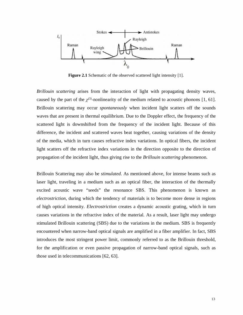
spectrum for spontaneous scattering from solid state matter. In inelastic scattering, the light
having a lower frequency than the incident light is called the Stokes branch, while the light
having a higher frequency than the incident light is called the anti-Stokes branch.
13
Figure 2.1 Schematic of the observed scattered light intensity [1].
Brillouin scattering arises from the interaction of light with propagating density waves,
caused by the part of the χ(3)-nonlinearity of the medium related to acoustic phonons [1, 61].
Brillouin scattering may occur spontaneously when incident light scatters off the sounds
waves that are present in thermal equilibrium. Due to the Doppler effect, the frequency of the
scattered light is downshifted from the frequency of the incident light. Because of this
difference, the incident and scattered waves beat together, causing variations of the density
of the media, which in turn causes refractive index variations. In optical fibers, the incident
light scatters off the refractive index variations in the direction opposite to the direction of
propagation of the incident light, thus giving rise to the Brillouin scattering phenomenon.
Brillouin Scattering may also be stimulated. As mentioned above, for intense beams such as
laser light, traveling in a medium such as an optical fiber, the interaction of the thermally
excited acoustic wave “seeds” the resonance SBS. This phenomenon is known as
electrostriction, during which the tendency of materials is to become more dense in regions
of high optical intensity. Electrostriction creates a dynamic acoustic grating, which in turn
causes variations in the refractive index of the material. As a result, laser light may undergo
stimulated Brillouin scattering (SBS) due to the variations in the medium. SBS is frequently
encountered when narrow-band optical signals are amplified in a fiber amplifier. In fact, SBS
introduces the most stringent power limit, commonly referred to as the Brillouin threshold,
for the amplification or even passive propagation of narrow-band optical signals, such as
those used in telecommunications [62, 63].

14
2.3 Spontaneous Brillouin Scattering
It is important to develop a macroscopic description of the light scattering process, whereby
the light scattering process occurs as a result of fluctuations in material density and
temperature. Assuming that the scattering volume, V, may be divided into smaller volumes,
V’, whereby all the atoms in V’ have the characteristic that they radiate in phase in the θ
direction. Letting Δϵ be the fluctuation of the dielectric constant in the volume V’, then we
have Δε = Δχ , where χ is the susceptibility of the material. This equality is deduced from the
relation ε = 1 + χ. Due to this change in optical susceptibility, an additional polarization is
developed, where 0~E is the electric field.
0~~ EP (2.1)
As a result, the dipole moment becomes
000~'~'~ EVPVp (2.2)
The change in dielectric constant can also be expressed as
TTT
(2.3)
It is also important to note that the electrostrictive constant of the material, γe, can be
expressed as
0
e (2.4)
From the field of acoustics [64], the equation of motion for a pressure wave is as follows
0~~'
~222
2
2
pv
tp
tp (2.5)
Here v is the velocity of sound inside the material, which is defined thermodynamically as
s
pv
2 (2.6)
And Γ' is the damping parameter, defined as
1
341'
pbs C
(2.7)

15
where ηs is the shear viscosity coefficient, ηb is the bulk viscosity coefficient, γ is the
adiabatic index, and κ is the thermal conductivity.
To illustrate the nature of the acoustic wave, we propose the following wave equation
..~ ccpep tqzi (2.8)
By substituting (2.8) into the equation (2.5), we see that q and are related by a dispersion
relation of the form
'222 ivq (2.9)
Which, after rearranging, can be written in the form
22
22 '1
vi
vq (2.10)
Which leads to the following expression
vi
vq
2
(2.11)
Where Г=ГB is the phonon decay rate, and is related to q in the following way
'2 qB (2.12)
In terms of Brillouin scattering, the phonon decay rate can also be expressed as the inverse of
the phonon lifetime, τB, as follows: ГB=1/τB. Assuming that the incident optical field obeys
the driven wave equation,
2
2
20
2
2
2
22
~1~~tP
ctE
cnE
(2.13)
and is described by the following expression
..,~00 cceEtzE ti rk (2.14)
combining the expressions (2.8) and (2.14), it becomes apparent that the scattered field obeys
the following wave equation

16
..
~~
02
*0
2
22
2
2
22
ccpeE
epEcC
tE
cnE
tirqki
tirqkise
(2.15)
Where Cs is the compressibility at constant entropy, and k is the wavevector. In the above
expression, the (ω-Ω) term leads to Stokes wave scattering, while the (ω+Ω) terms leads to
anti-Stokes scattering.
In Stokes scattering, the scattered wavevector, k2, may be expressed in terms of the incident
and acoustic wavevector, k1, and q, as follows: k2 = k1 - q, having a frequency ω2 = ω1 - Ω.
The frequency and wavevector of the incident field, ω1 and k1, are related by: ω1 = |k1|c/n,
while the frequency and wavevector of the acoustic wave, Ω and q, are related as follows: Ω
= |q|v.
Efficient scattering can occur only if the frequency and wavevector of the scattered wave, ω2
and k1, are related by the dispersion relation for optical waves, namely: ω2 = |k2|c/n.
Stokes scattering is illustrated on Figure 2.2 below, with scattering angle θ.
Figure 2.2. Stokes Brillouin scattering [1].
(a) Relative orientations of the wavevectors k1 and k2, (b) k1, k2 and q relationship,
(c) Schematic of SBS interaction.

17
Since |k1| ≈ |k2|, we have the following relation: |q| = 2|k1|sin(θ/2). According to the
dispersion relation Ω = |q|v, we therefore have the following expression for the acoustic
frequency
Ω1 = 2nω1(v/c)sin(θ/2) (2.16)
Taking into account that the majority of scattering occurs for θ=180°, the maximum
frequency shift becomes: ΩB = 2nω1(v/c). As such, Stokes scattering can be visualized from
a retreating acoustic wave.
The same analysis may be applied to the case of anti-Stokes scattering. The scattered
wavevector, k3, may be expressed in terms of the incident and acoustic wavevectors, k1, and
q, as follows: k2 = k1 + q, having a frequency ω3 = ω1 + Ω. As before, efficient scattering
can occur only if the frequency and wavevector of the scattered wave, ω3 and k1, are related
by the dispersion relation for optical waves, namely: ω3 = |k3|c/n.
Anti-Stokes scattering is illustrated on Figure 2.3 below, with scattering angle θ.
Figure 2.3. Anti-Stokes Brillouin scattering [1].
(a) Relative orientations of the wavevectors k1 and k3, (b) k1, k3 and q relationship,
(c) Schematic of SBS interaction.
18
Since |k1| ≈ |k3|, we once again have the following relation: |q| = 2|k1|sin(θ/2). According to
the dispersion relation Ω = |q|v, we therefore have the same expression for acoustic
frequency as in expression (2.16)
Ω2 = 2nω1(v/c)sin(θ/2) (2.17)
Taking into account that the majority of scattering occurs for θ=0° for anti-Stokes scattering,
the maximum frequency shift becomes: ΩB=2nω1(v/c). Anti-Stokes scattering can be
visualized from an oncoming acoustic wave.
2.4 Stimulated Brillouin Scattering
The previous section 2.3 discussed the mechanisms of spontaneous Brillouin scattering,
where the applied optical fields were sufficiently weak to leave the acoustic properties of the
material unaltered. However, if the laser light is sufficiently intense, the incident and
scattered field can beat together, creating a dynamic acoustic grating via electrostriction. The
incident field will then scatter off the acoustic grating at the Stokes frequency and add
constructively with the scattered, Stokes or anti-Stokes, field. In this way, the amplitudes of
the acoustic grating and scattered light are reinforced. Though the χ(3)-nonlinearity of a
medium is rather small, Brillouin scattering can grow exponentially to a large amplitude in
optical fibers.
2.4.1 SBS Generator
There exist two conceptually different configurations in which SBS can be studied [1].
Figure 2.4 shows the configuration of the SBS generator, in which only the laser beam is
applied externally, a pump wave with frequency ω1, while both the Stokes wave with
frequency ω2, and the acoustic wave, are created from the noise within the region of
interaction. The noise is typically generated by the scattering of pump laser light from
thermally-generated density fluctuations (phonons).

19
Figure 2.4 SBS generator [1].
2.4.2 SBS Amplifier
Figure 2.5 shows the configuration for a SBS amplifier, in which both the laser and Stokes
fields are applied externally. In this configuration, the pump and Stokes fields are counter-
propagating, and a strong interaction takes place when the frequency of the injected Stokes
wave is equal to that which would be created by the SBS generator. In this manuscript, the
SBS amplifier configuration will be considered.
Figure 2.5 SBS amplifier [1].
2.4.3 Electrostriction
Electrostriction is the tendency of materials to acquire a higher overall density in the
presence of an applied electric field. Certain third-order optical responses are caused by the
electrostriction phenomenon, including stimulated Brillouin scattering (SBS) which is the
focus of this thesis.
We can explain the origin of this effect by taking a look at the change in potential energy per
unit volume of a material placed in the presence of an electric field E.
202
1 Eu (2.18)
Here is the relative dielectric constant, and 0 is the permittivity of free space. In the
presence of the electric field E
, each molecule experiences a dipole moment

20
Ep
0 (2.19)
Where is the molecular polarizability. It follows that the energy of the molecule is
E
EEdpU
0
202
1' (2.20)
As such, the resultant force acting on the molecule is given by
202
1 EUF
(2.21)
From expression (2.21), it is apparent that the force acting on the molecule pulls it into the
region of increasing electric field strength. Hence, an applied electric field E
onto a material
will result in the molecules of the material, at the vicinity of the applied force, to be pulled in
the direction of increasing field strength. As such, the density in this vicinity will increase, in
turn causing the local index of refraction to change as well. The result is a dynamic acoustic
grating along the length of the fiber, characterized by periodic differences in density, and
consequently the index of refraction.
2.4.4 SBS Coupled wave equations and configuration
The previous section 2.4.3 described the mechanism of electrostriction by which the
dynamic acoustic grating, inherent in stimulated Brillouin scattering, is created. In this
section, we will describe the possible configurations of the laser lights and fiber which allow
us to attain the electrostriction effect most efficiently, and derive the standard coupled wave
equations related to each configuration.
An incident electric field at a certain frequency scatters off the refractive index variations,
the scattered light being at the same frequency as the incident light. As such, the scattered
light interacts constructively with the incident pulse which originally produced the acoustic
disturbance, both mutually reinforcing each other’s existence. The incident pulse, which may
be either a Stokes or an anti-Stokes wave, is launched into the beginning of the fiber z=0,
where z is the coordinate inside the fiber. The pump wave (PW) is launched into the opposite
end of the fiber z=L, where L is the total length of the fiber. This configuration is shown on
Figure 2.6 below.

21
Figure 2.6 Schematic arrangement of SBS in a fiber of length L.
Pump and probe configuration: A1(z) – Pump wave, A2(z)– probe wave (incident pulse).
Firstly, we consider the case when the incident pulse has a downshifted frequency as
compared to the frequency of the PW, by a frequency of ΩB=10-11 GHz, also known as the
Brillouin frequency. Such a pulse is called the Stokes wave (SW), and is responsible for
Brillouin gain in the SBS amplifier.
We begin with the equations representing the incident waves involved in the Brillouin
interaction.
..,,~11
11 ccetzAtzE tzi k (2.22)
..,,~22
22 ccetzAtzE tzi k (2.23)
Where 1~E represents the pump wave incident at the end of the fiber, and 2
~E represents the
pulse incident at the beginning of the fiber, or Stokes wave. k1, k2 are the wavevectors of the
pump wave (PW) and Stokes waves (SW) respectively, and ω1 and ω2 are the frequencies of
the PW and SW respectively. The acoustic wave may be expressed in terms of material
density distribution, where Ω = ω1 - ω2, q≈2k1, and ρ0 denotes the density of the material.
..,,~ 1101 ccetztz tzi q (2.24)
The scattered field obeys the wave equation
2
2
20
2
2
2
22
~1~~tP
ctE
cnE ii
i
, i=1,2 (2.25)

22
Where the polarization iP~ of the medium is given in terms of the electrostrictive constant, e ,
the permittivity of free space, 0 , mean density of the material ρ0, and in terms of density
),(~ tz .
tzEtztrP e ,~,~,~0
0
(2.26)
The equation of motion for a pressure wave, which we have used to describe the propagation
of the acoustic wave inside the fiber, follows the acoustic wave equation
0~~'
~222
2
2
pv
tp
tp (2.27)
Here v is the velocity of sound inside the material, Γ' is the damping parameter, defined as
ΓB=q2Γ', where ГB=1/τB is the inverse of the phonon lifetime, τB. Substituting equations
(2.22)-(2.23) into (2.25) and equation (2.24) into (2.27), we get the following system of
equations describing the interaction of the pump, Stokes and acoustic waves.
1210
111
21
2/1 AA
nci
tA
nczA e
(2.28)
21*
10
122
21
2/1 AA
nci
tA
nczA e
(2.29)
*21
21
1121
2
4AAqi e
BB (2.30)
Where α is the fiber attenuation parameter, and q has been denoted as q1, and ρ has been
denoted as ρ1. The following approximations have been made to attain this system of
equations: the phonon propagation distance is considered to be small compared to the
distance over which the amplitude of the acoustic wave fluctuates [1]. For the optical waves,
the slowly-varying amplitude approximation has been applied.

23
Figure 2.7 Schematic distribution of the pump and probe intensities during SBS [1].
Figure 2.7 above shows a typical intensity distribution of the pump and Stokes powers inside
an optical fiber, in the steady state regime of SBS.
The incident pulse may also have an upshifted frequency as compared to the frequency of the
PW, such a pulse is called the anti-Stokes wave (ASW), and is responsible for Brillouin loss
in the SBS amplifier. The same analysis may be applied to obtain equations for this case, and
the result will be very similar to the system of equations (2.28)-(2.30), with the difference
that the Stokes wave parameters will be replaced by corresponding anti-Stokes parameters.
In fact, from a physical point of view, since the PW is now downshifted from the ASW by
the Brillouin frequency, the anti-Stokes may be viewed as a new ‘pump wave’ and the PW
may be viewed as a new ‘Stokes wave’.
2.4.5 Combined Brillouin gain and loss coupled wave equations and configuration
In this section we will derive the equations governing the SBS interaction for the case of
simultaneous gain and loss. Following section 2.4.4, we may add an additional wave,
representing the anti-Stokes wave to the pump and Stokes waves described by equations
(2.22) and (2.23):
..,,~33
33 ccetzAtzE tzki (2.31)
and an additional acoustic field, which results from the interaction of the PW and ASW
..,,~ 2202 ccetztz tqzi (2.32)
24
Repeating the analysis of section 2.4.4, we get the following system of equations, describing
the interaction of the PW, SW, ASW and two acoustic waves [1, 65].
13*2
0
121
0
11
21
22AA
nciA
nci
dzdA ee
(2.33)
21*1
0
22
21
2AA
nci
dzdA e
(2.34)
3120
33
21
2AA
nci
dzdA e
(2.35)
*21
21
1121
2
4AAqi e
BB (2.36)
*13
22
2222
2
4AAqi e
BB (2.37)
Where Ω1=ω1 – ω2, Ω2=ω3 – ω1, q1 and q2 are the acoustic wavevectors defined as q1=k1-
k2≈2k1 and q2=k3-k1≈2k1, where k1, k2 and k3 are the wavevectors of the PW, SW and ASW
respectively, defined as cnk ii /
, i=1,2,3.
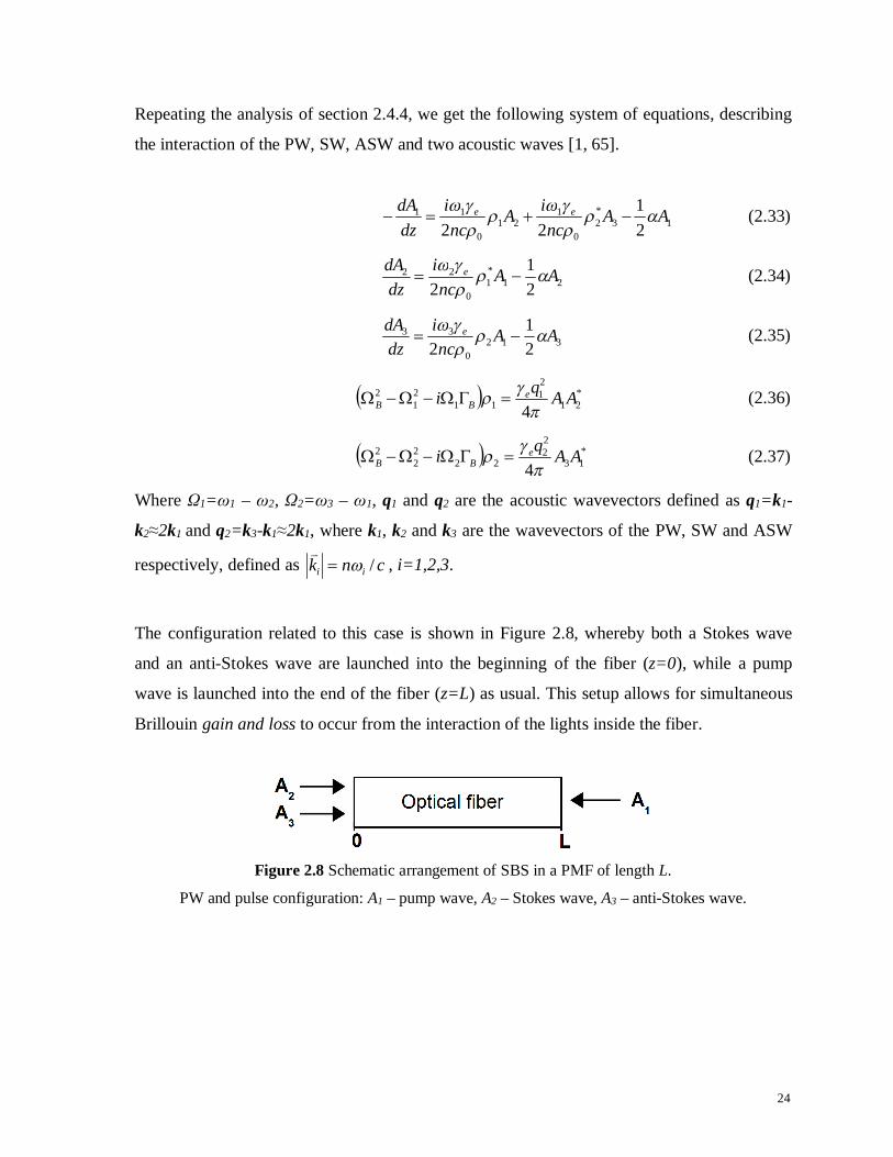
The configuration related to this case is shown in Figure 2.8, whereby both a Stokes wave
and an anti-Stokes wave are launched into the beginning of the fiber (z=0), while a pump
wave is launched into the end of the fiber (z=L) as usual. This setup allows for simultaneous
Brillouin gain and loss to occur from the interaction of the lights inside the fiber.
Figure 2.8 Schematic arrangement of SBS in a PMF of length L.
PW and pulse configuration: A1 – pump wave, A2 – Stokes wave, A3 – anti-Stokes wave.

25
2.5 Polarization and birefringence
2.5.1 Polarization states
Polarization is a property of waves which can oscillate with more than one orientation [66,
67, 68]. Electromagnetic waves, such as light, exhibit polarization whereby the electric field
vector traces out an ellipse. The shape and orientation of this ellipse (or line) defines the
polarization state. The following Figure 2.9 shows some examples of the evolution of the
electric field vector, with time (the vertical axes), at a particular point in space, along with its
x and y components.
Linear
(a)
Circular
(b)
Elliptical
(c)
Figure 2.9 Different polarization states, figure taken from Wikipedia.
In Figure 2.9(a), the electric field's x and y components are exactly in phase. The net result is
polarization along a particular direction in the x-y plane over each cycle. Since the vector
traces out a single line in the plane, this special case is called linear polarization. In Figure
2.9(b), the x and y components maintain the same amplitude but now are exactly 90° out of
phase. In this special case, the electric field vector traces out a circle in the plane, and is thus
referred to as circular polarization. Depending on whether the phase difference is + or −90°,
it may be qualified as right-hand circular polarization or left-hand circular polarization.
26
The most general case occurs when the x and y components are out of phase by an arbitrary
amount, or 90° out of phase but with different amplitudes, and is called elliptical
polarization. In this case, the electric field vector traces out an ellipse (the polarization
ellipse). This case is depicted in Figure 2.9(c). The ellipse shape may be produced either by a
clockwise or counterclockwise rotation of the field, corresponding to distinct polarization
states.
In summary, in the most general case, the optical field E
is elliptically polarized, but there
exist several combinations of amplitudes and phases which describe particular cases of
polarization. These states of polarization are called degenerate polarization states: linearly
horizontal/vertical polarized light (LHP/LVP), linear ±45° polarized light (L+45P/L-45P),
and right/left circularly polarized light (RCP/LCP).
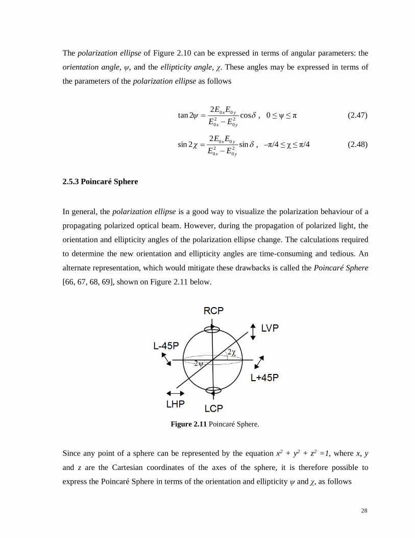
2.5.2 Polarization ellipse
According to Fresnel’s theory [66], orthogonal components of a field E
may be expressed by
wave equations
2
2
22 ,1,
ttzE
ctzE x
x
(2.38)
2
2
22 ,1,
ttzE
ctzE y
y
(2.39)
Where Ex(z,t) and Ey(z,t) are the optical field components, which describe sinusoidal
oscillations in the x-z and y-z planes, c is the velocity of propagation of the optical field in
space, and t is time. The simplest solution of equations (2.38) and (2.39) is in terms of
sinusoidal functions. For propagation in the +z-direction, the solutions may be represented as
xxx kztEtzE cos, 0 (2.40)
yyy kztEtzE cos, 0 (2.41)

27
Where E0x and E0y are the maximum amplitudes, ωt-kz is the propagator, and δx and δy are
arbitrary phases of the components respectively. Equations (2.40) and (2.41) can be re-
written in the following way
xxx
x kztkztE
tzE sinsincoscos,
0
(2.42)
yyy
y kztkztE
tzE sinsincoscos
,
0
(2.43)
After some algebra, the following relations can be derived
xyxy
yy
x
x kztE
tzEE
tzE sincossin,
sin,
00
(2.44)
xyxy
yy
x
x kztE
tzEE
tzE sincoscos,
cos,
00
(2.45)
By squaring equations (2.44) and (2.45) and adding them together, the following equation is
obtained
2
002
0
2
20
2
sincos,,2,,
yx
yx
y
y
x
x
EEtzEtzE
EtzE
EtzE (2.46)
where δ = δx - δy and δx and δy are arbitrary phases. Equation (2.46) is referred to as the
polarization ellipse, which represents a locus of points described by the optical field as it
propagates. A schematic diagram of the polarization ellipse is shown in Figure 2.10.
Figure 2.10 Polarization Ellipse.
28
The polarization ellipse of Figure 2.10 can be expressed in terms of angular parameters: the
orientation angle, ψ, and the ellipticity angle, χ. These angles may be expressed in terms of
the parameters of the polarization ellipse as follows
cos2
2tan 20
20
00
yx
yx
EEEE
, 0 ≤ ψ ≤ π (2.47)
sin2
2sin 20
20
00
yx
yx
EEEE
, –π/4 ≤ χ ≤ π/4 (2.48)
2.5.3 Poincaré Sphere
In general, the polarization ellipse is a good way to visualize the polarization behaviour of a
propagating polarized optical beam. However, during the propagation of polarized light, the
orientation and ellipticity angles of the polarization ellipse change. The calculations required
to determine the new orientation and ellipticity angles are time-consuming and tedious. An
alternate representation, which would mitigate these drawbacks is called the Poincaré Sphere
[66, 67, 68, 69], shown on Figure 2.11 below.
Figure 2.11 Poincaré Sphere.
Since any point of a sphere can be represented by the equation x2 + y2 + z2 =1, where x, y
and z are the Cartesian coordinates of the axes of the sphere, it is therefore possible to
express the Poincaré Sphere in terms of the orientation and ellipticity ψ and χ, as follows

29
x = cos(2χ)cos(2ψ) (2.49)
y = cos(2χ)sin(2ψ) (2.50)
z = sin(2χ) (2.51)
Equation (2.49)-(2.51) relate the Cartesian coordinates (x, y, z) to the Poincaré Spherical
coordinates (1, ψ, χ).
Applying the time average definition to the polarization ellipse of equation (2.46) yields the
following equation
2002
0022
020
220
20 sin2cos2 yxyxyxyx EEEEEEEE (2.52)
Defining the terms of equation (2.52) in the following way
20
200 yx EES (2.53)
20
201 yx EES (2.54)
cos2 002 yxEES (2.55)
sin2 003 yx EES (2.56)
We obtain the following relation23
22
21
20 SSSS (2.57)
Where S0, S1, S2 and S3 are the observables of the polarized field, and are called the Stokes
polarization parameters. The S0 parameter describes the total intensity of the optical beam,
which is usually normalized to 1. The S1 parameter describes the domination of LHP light
over LVP, the S2 parameter describes the domination of L+45P light over L-45P light, while
the S3 parameter describes the domination of RCP light over LCP.

30
The normalized Stokes vector may be expressed as S=(S1, S2, S3), and may be used to express
degenerate polarization states as follows: SLHP=(1,0,0), SLVP=(-1,0,0), SL+45P=(0,1,0), SL-
45P=(0,-1,0), SRCP=(0,0,1), and SLCP=(0,0,-1). An elliptically polarized light will have a
Stokes vector whereby S1, S2, S3 ≠ 0, while a first order approximation to unpolarized light
will have a Stokes vector S=(0,0,0).
2.5.4 Birefringence
Birefringence is an optical property of a material having a refractive index which depends on
the polarization and propagation direction of light [1, 61]. The birefringence is often
quantified as the maximum difference between refractive indices exhibited by the material.
In optical fibers, birefringence results from the difference in indices of refraction between the
two principal x- and y- axes, also referred to as the fast and slow axes, since light will
propagate with different speeds along two axes having different indices of refraction.
Intrinsic birefringence results from asymmetry of the fiber core, usually caused by
imperfections of the fiber drawing process. Induced birefringence results from induced stress
on the fiber, such as bending or twisting. For all practical purposes, the fiber manufactured
would possess a various degree of birefringence either due to imperfections in the fiber
drawing process, or in the later cabling and installation processes, as well as environmental
perturbations. The different kinds of birefringence include linear birefringence, which causes
the orthogonally polarized modes to have linear polarizations (LP). Circular birefringence
produces left- and right-circularly polarized (CP) modes, while elliptical birefringence
causes elliptical polarization of the orthogonally polarized modes. The difference in
refractive indices of the principle axes causes the light to travel along orthogonally polarized
modes at different phase velocities, yielding a phase difference between the two waves. The
two waves will arrive at the end of the fiber at different times, causing the output spectrum of
light to spread out, resulting in polarization mode dispersion (PMD). The length of the fiber
required to bring the two polarization modes back in phase and reproduce the original
polarization state is the beat length, LB, defined as LB = λ/Δn, where λ is the wavelength of
light, and n is the refractive index.

31
2.6 Summary
In conclusion, nonlinear optics studies the interaction between moderate and intense optical
fields. When light travels through matter, various scatterings, which are caused by
fluctuations of the optical properties of the medium can occur. The spontaneous Brillouin
scattering arises from the interaction between a light wave and an acoustic wave. The
acoustic wave can be considered as a propagating grating that diffracts the incident wave and
induces the periodic variation of the material density, and consequently, the refractive index
change. The diffracted wave experiences a frequency shift with an amount proportional to
the acoustic velocity inside the material due to the Doppler Effect. Stimulated Brillouin
scattering arises from the electrostriction caused by the incident optical fields. When two
counter-propagating light waves are present inside the fiber, the beating of these two waves
can induce the density and refractive index variation caused by electrostriction. The acoustic
wave inside the fiber is enhanced when the beat frequency of the two lightwaves matches
with the frequency of the acoustic wave. The scattered Stokes wave is then increased by the
enhanced acoustic wave. The positive feedback between the acoustic wave and the scattered
Stokes wave leads to Stimulated Brillouin scattering. This mechanism can also include both
the Stokes and anti-Stokes waves, to yield combined Brillouin gain and loss in an optical
fiber. In this regime, there are two scattered waves, the SW and the ASW, and two counter-
propagating acoustic gratings inside the optical fiber.
Since SBS originates from the mixing of the two light waves, the efficiency of this effect is
polarization dependent. Polarization states arise from the oscillation of the electric field with
different orientations in a polarization ellipse. A Poincaré sphere is used to derive Stokes
vectors, which are used to define polarization states. Birefringence is an optical property of a
material having a refractive index which depends on the polarization and propagation
direction of light, and is defined as the maximum difference between the refractive indices
exhibited by the material. In optical fibers, this is the difference between the indices of
refraction of the x- and y- principal states of polarization.
32
Chapter 3
3D parametric model
3.1. Introduction
As described in section 1.2, previously obtained solutions for SBS are numerical with
analytical portions, and, therefore, qualify as hybrid solutions. Though the analytical portions
provide useful information about intensity distributions along the fiber, they fall short in
describing spectral characteristics of the Brillouin amplification conveyed by the
transcendental equation. The lack of analytical expressions for Brillouin spectra substantially
limits the utility of the hybrid solution [8] for applications, since spectral measurement is a
leading technique for strain and temperature sensing. Methods of avoiding systematic errors
in distributed fiber sensing are described in [3, 70, 71, 72], but do not include the correct
conditions under which an undesirable effect of spectral distortion occurs in optical fibers,
nor how to more accurately obtain a Lorentzian profile for sensing applications.
We propose a 3D parametric model of Brillouin amplification that will reflect the effects of
input pump and pulse powers on the level of pump wave depletion in the lossless fiber, and
act as a classification tool to describe the level of similarity between various Brillouin
amplification processes in optical fibers. This model is valid in any power regime capable of
sustaining SBS, corresponding to 0<Ppump<10mW and 0<PStokes<40mW, and for an arbitrary
depletion of the PW and pulses, acting as an effective, universal, tool for avoiding the
undesirable spectral distortion via limitations of the parameter space that is relevant to
distributed Brillouin fibers.
Additionally, the 3D parametric model has been used to find fully analytic solutions for
calculating the distribution of a pump wave (PW), which has been taken to be a continuous
wave, and a Stokes wave (SW) intensities and phases, for an arbitrary pump depletion
(0-100%), and an arbitrary range of pump and pulse intensities, in fiber lengths of up to a

33
few kilometers. These solutions are valid for expressing the Brillouin spectrum under
different depletion conditions, including the spectral distortion effect that occurs for high
levels of pump depletion and high Stokes powers, which has been confirmed experimentally.
3.2 Model
The process of stimulated Brillouin scattering has been studied in a lossless single mode
optical fiber, with core radius of 4.1μm. Attenuation terms have been neglected due to the
short fiber lengths inherent in the model. The schematic arrangement and typical intensity
distributions are shown on Figures 2.6 and 2.7 in Chapter 2.
In the slowly varying amplitude approximation, recall that the steady state interaction
between the PW, the SW and an acoustic wave (AW1) is described by the following system
of equations [9]. The system operates in the steady-state regime when pulse lengths greater
than 10ns.
210
11
2A
nci
zA e
(3.1)
1*1
0
22
2Aρ
ncργiω=
zA e
(3.2)
*21
21
1121
2
4AAqi e
BB
(3.3)
Where:Ω1=ω1 - ω2
A1 – complex amplitude of the PWA2 – complex amplitude of the SWρ1 – complex amplitude of the AW1
caused by interaction of PW + SWω1 – angular frequency of the PWω2 – angular frequency of the SWγe – electrostrictive constantz – coordinate along the fiberq1 – acoustic wavevector: q1≈2k1
Ω1 – angular frequency of the AW1
caused by interaction of PW + SW
ΩB – Brillouin frequency: 12n ωcv=ΩB
c – speed of lightρ0 – density of the fiberΓB – Brillouin linewidthv – speed of sound in the fibern – index of refraction of the fiberk1 – wavevector of the PW: |k1|=nω1/c

34
Recall that in the above arrangement, the SW input parameters are known only at the
beginning of the fiber, i.e. at z=0. Correspondingly, the PW input parameters are known only
at the end of the fiber, i.e. at z=L, where L is the length of the fiber. Therefore, the boundary
conditions for system of equations (3.1)-(3.3) are as follows
|A1(L)|2 = A210; |A2(0)|2 =A220 (3.4)
where A210 and A220 are known squared absolute values of the complex amplitudes A1 and A2,
respectively.
The goal is to find analytical expressions for the intensities and phases of the PW and SW.
Introducing the intensities of the waves as 22π ii Anc=I , where Ii is the intensity of the i-th
wave, the system of equations (3.1)-(3.3) is transformed into the following system of
equations (3.5)-(3.7).
212110
3
321
112 II
cnk
dzdI
B
e
(3.5)
212110
3
322
112 II
cnk
dzdI
B
e
(3.6)
2121
2
10
22
1 112 II
nck
B
e
(3.7)
B
B
ΓΩΩΩ=ξ
1
21
2
1 (3.8)
Equations (3.5)-(3.7) are similar to those derived in [8]. Correspondingly, the boundary
conditions (3.4) become as follows, where I10 and I20 are the input intensities of the PW and
SW respectively
|I1|2z=L= I10; |I2|2z=0=I20 (3.9)
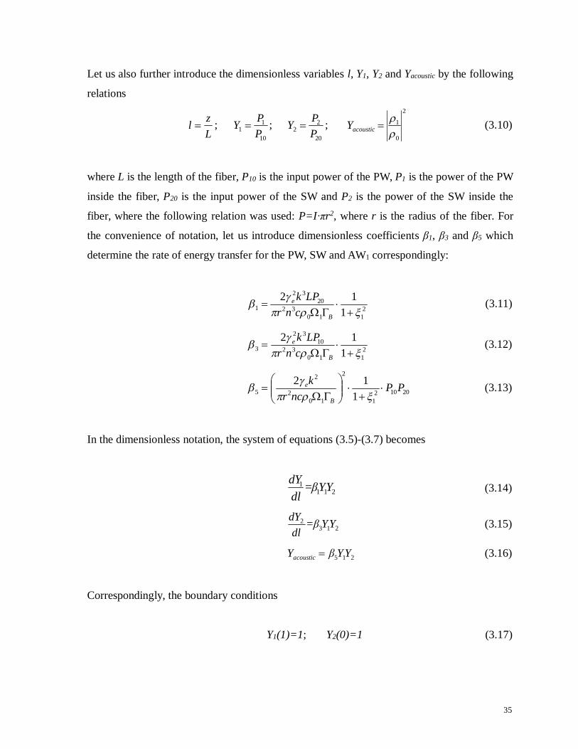
35
Let us also further introduce the dimensionless variables l, Y1, Y2 and Yacoustic by the following
relations
Lzl ;
10
11 P
PY ;20
22 P
PY ;2
0
1
acousticY (3.10)
where L is the length of the fiber, P10 is the input power of the PW, P1 is the power of the PW
inside the fiber, P20 is the input power of the SW and P2 is the power of the SW inside the
fiber, where the following relation was used: P=I∙πr2, where r is the radius of the fiber. For
the convenience of notation, let us introduce dimensionless coefficients β1, β3 and β5 which
determine the rate of energy transfer for the PW, SW and AW1 correspondingly:
2110
3220
32
1 112
B
e
cnrLPk (3.11)
2110
3210
32
3 112
B
e
cnrLPk (3.12)
201021
2
102
2
5 112 PP
ncrk
B
e
(3.13)
In the dimensionless notation, the system of equations (3.5)-(3.7) becomes
2111 YY=β
dldY
(3.14)
2132 YY=β
dldY (3.15)
215 YYβYacoustic (3.16)
Correspondingly, the boundary conditions
Y1(1)=1; Y2(0)=1 (3.17)

36
3.3 Solution
The following analysis will be performed on the system of equations (3.14)-(3.16) to
determine the dimensionless intensities Y1 and Y2 of the interacting optical waves, in a similar
way to the one performed in [8].
Since β3≠0, we can find the product of Y1 and Y2 from equation (3.15), and substitute the
product into equation (3.14), determining thereby the first integral of the system
123
11 C=Y
ββY (3.18)
Determining the arbitrary constant C1 from the boundary conditions (3.17) at ℓ=0, we yield
3
111 0
ββY=C (3.19)
where Y1(0) is the output intensity of the PW. Finding Y2 from the first integral (3.18) and
substituting it into equation (3.14), we yield the following differential equation for Y1
11131 CYY=β
dldY
(3.20)
Since Y2(ℓ) is a monotonically increasing function of its argument, starting from Y2(0)=1, and
assuming that the PW is never depleted completely, we conclude that Y1≠0 and Y2≠0 for any
ℓ∊[0, 1]. Therefore, it follows from (3.18) that Y1-C1 ≠ 0. This allows for separation of
variables in (3.20), resulting in the following second integral of the system of equations
(3.14)-(3.16).

37
∫ dY 1
Y 1⋅(Y 1−C1)=∫β3⋅dl+ C3 (3.21)
Determining the arbitrary constant C3 from the boundary conditions (3.17) and introducing a
dummy variable τ, we yield
lβ=
l Cττdτ
Y
1
13
11
(3.22)
Expression (3.22) contains the yet unknown output intensity Y1(0) of the PW as a part of the
arbitrary constant C1. At ℓ=0, the expression (3.22) turns into a nonlinear equation for
determining Y1(0)
3
13
11
1
0 0β=
ββ+Yττ
dτ
Y
(3.23)
Once Y1(0) is determined from (3.23) and Y1(ℓ) is determined from (3.22), Y2(ℓ) can be found
from the first integral (3.18) as follows
10111
32 +YlY
ββ=lY (3.24)
Here we will only consider the case when C1≠0. The integrand can be expanded into a sum
of simple fractions, each fraction being continuous on the interval of integration [Y1(ℓ), 1].
τCτC=
Cττ1111
111; C1≠0 (3.25)
Integration and further simplification yield
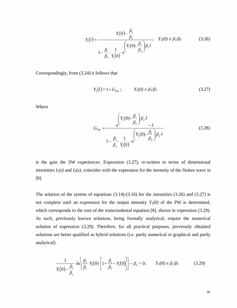
38
lβββY
Yββ
ββY
=lY
33
11
13
1
3
11
1
)0(e
011
0; Y1(0) ≠ β1/β3 (3.26)
Correspondingly, from (3.24) it follows that
SWG=lY 12 ; Y1(0) ≠ β1/β3 (3.27)
Where
lβββY
Yββ
lβββY
GSW
33
11
13
1
33
11
)0(e
011
1)0(
e (3.28)
is the gain the SW experiences. Expression (3.27), re-written in terms of dimensional
intensities I1(z) and I2(z), coincides with the expression for the intensity of the Stokes wave in
[8].
The solution of the system of equations (3.14)-(3.16) for the intensities (3.26) and (3.27) is
not complete until an expression for the output intensity Y1(0) of the PW is determined,
which corresponds to the root of the transcendental equation [8], shown in expression (3.29).
As such, previously known solutions, being formally analytical, require the numerical
solution of expression (3.29). Therefore, for all practical purposes, previously obtained
solutions are better qualified as hybrid solutions (i.e. partly numerical or graphical and partly
analytical).
0010ln
0
131
3
11
1
3
3
11
=βYββ+Y
ββ
ββY
; Y1(0) ≠ β1/β3 (3.29)
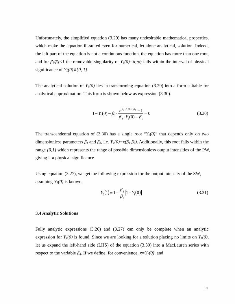
39
Unfortunately, the simplified equation (3.29) has many undesirable mathematical properties,
which make the equation ill-suited even for numerical, let alone analytical, solution. Indeed,
the left part of the equation is not a continuous function, the equation has more than one root,
and for β1/β3<1 the removable singularity of Y1(0)=β1/β3 falls within the interval of physical
significance of Y1(0)∊(0, 1].
The analytical solution of Y1(0) lies in transforming equation (3.29) into a form suitable for
analytical approximation. This form is shown below as expression (3.30).
0)0(
1)0(1113
)0(
11
113
YeY
Y
(3.30)
The transcendental equation of (3.30) has a single root “Y1(0)” that depends only on two
dimensionless parameters β1 and β3, i.e. Y1(0)=x(β1,β3). Additionally, this root falls within the
range [0,1] which represents the range of possible dimensionless output intensities of the PW,
giving it a physical significance.
Using equation (3.27), we get the following expression for the output intensity of the SW,
assuming Y1(0) is known.
0111 11
32 YY
(3.31)
3.4 Analytic Solutions
Fully analytic expressions (3.26) and (3.27) can only be complete when an analytic
expression for Y1(0) is found. Since we are looking for a solution placing no limits on Y1(0),
let us expand the left-hand side (LHS) of the equation (3.30) into a MacLauren series with
respect to the variable β3. If we define, for convenience, x=Y1(0), and

40
13131
11),,(13
xexxF
x
Then xexF 1),0,( 1 , and n
nn
n
xCexFn
1
3
1 ),0,(!
1
where
n
n
nn
eC
1
11 !1...11
The corresponding MacLauren series is
n
n
nn xCexexF 3
131
11),,(
Thus, the equation (3.30) takes a form suitable for finding approximate analytical solutions.
031
11
n
n
nn xCexe (3.32)
3.4.1 Linear approximation
Keeping only linear terms in (3.32) we yield the simplest approximation as follows
011
13
111
xeexe
Collecting like terms and solving for “x” yields
1331
1
11
ex (3.33)

41
If better accuracy is required, the quadratic approximation is in order.
3.4.2 Quadratic approximation
Keeping additionally β32 terms in (3.32), we yield the next approximation as follows
0211
1 22
1
211
23
1
13
1
11
11
xe
exeexe
After some simple but tedious algebra, we obtain a more accurate expression for the output
intensity of the PW.
21
2112
32 2
11
41
21
1
1
e
x
xx
linear
linear (3.34)
where xlinear is the output intensity of the PW in the linear approximation, defined by (3.33).
In a similar way, one can also get the cubic and quartic approximations, which we do not
show here due to their complexity.
3.5 Relative error
To gauge the accuracy of our analytical solutions (3.33) and (3.34), we compare them to the
numerically calculated solution for the output dimensionless PW intensity. The
transcendental equation (3.30) lends itself to numerical solution with the use of standard
methods of computational physics.

42
3.5.1 Linear Approximation
The relative error is less than 33% in the worst case, on the interval 0<β1<25.4, 0<β3<6.4, in
this case, corresponding to 0<Ppump<10mW , 0<PStokes<40mW, as it is shown on Figure 3.1
below.
Figure 3.1 Relative error of Y1(0): Linear Approximation of 3D parametric model of output PW.
L=1000m, 0<Ppump<10mW , 0<PStokes<40mW
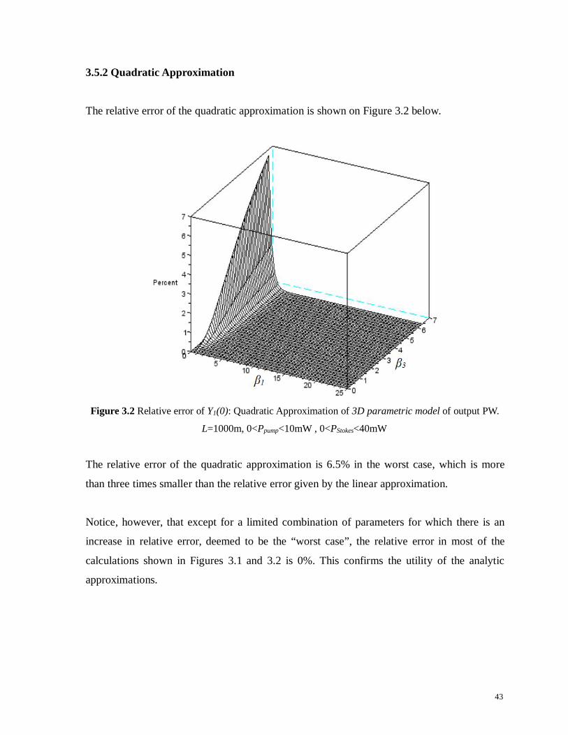
43
3.5.2 Quadratic Approximation
The relative error of the quadratic approximation is shown on Figure 3.2 below.
Figure 3.2 Relative error of Y1(0): Quadratic Approximation of 3D parametric model of output PW.
L=1000m, 0<Ppump<10mW , 0<PStokes<40mW
The relative error of the quadratic approximation is 6.5% in the worst case, which is more
than three times smaller than the relative error given by the linear approximation.
Notice, however, that except for a limited combination of parameters for which there is an
increase in relative error, deemed to be the “worst case”, the relative error in most of the
calculations shown in Figures 3.1 and 3.2 is 0%. This confirms the utility of the analytic
approximations.

44
3.6 3D parametric model
An analytic 3D parametric model, attained by plotting the linear approximation solution as a
function of dimensionless parameters β1 and β3 is shown in Figure 3.3 below.
Figure 3.3 Linear Approximation of Y1(0): 3D parametric model of output PW.
Dimensionless output intensity of the PW versus dimensionless parameters β1 and β3.
γe=0.902, v=5616 m/s, n=1.48, λ=1.319μm, ρ0=2.21 g/cm3, ΓB = 0.1 GHz
L=1000m, 0<Ppump<10mW , 0<PStokes<40mW
As can be seen from Figure 3.3, the linear approximation (3.34) covers the entire range of
values of output intensities of the PW (i.e. from weak depletion, to full depletion when
Y1(0)~0). In spite of its simplicity, this 3D parametric model is valid in a wide range of
combinations of dimensionless parameters β1 and β3.
Using equation (3.31), a similar 3D parametric model for the output Stokes intensity is
calculated and shown below in Figure 3.4.

45
Figure 3.4 Linear Approximation of Y2(ℓ): 3D parametric model of output SW.
Dimensionless output intensity of the SW versus dimensionless parameters β1 and β3.
γe=0.902, v=5616 m/s, n=1.48, λ=1.319μm, ρ0=2.21 g/cm3, ΓB = 0.1 GHz
L=1000m, 0<Ppump<10mW , 0<PStokes<40mW
As expected, while the PW experiences depletion, the SW experiences amplification.
3.7 3D parametric model: Similar and Dis-similar Processes
The 3D parametric model for the output PW intensity allows for the easy interpretation of
the effects of pump and pulse powers on the level of PW depletion in the fiber. Parameters of
the fiber are described in Figures 3.3 and 3.4, and the range of pump and Stokes powers
0<Ppump<10mW, 0<PStokes<40mW, correspond to the following range of dimensionless
parameters β1 and β3: 0<β1<6.4 ; 0<β3<25.4. This power range models PW depletion from
0-100%, corresponding to 0<Y1(0)<1 from Figure 3.1. For example, restricting the range of
SW power to 1.6 mW<PStokes<40 mW yields a depletion of 55-100%. Further changes in SW
power change the level of depletion accordingly. Being a very versatile model, a change in
Stokes power, parameters of the fiber, or fiber length would alter the restrictions on β1 and β3,

46
therefore allowing for the “picking and choosing” of the preferred level of depletion for the
given fiber. For example, in optical fibers it is often preferable to avoid large depletion,
which would require a Stokes power of <1.6mW for the parameters given in Figures 3.3 and
3.4.
The study of analytical solutions for the output PW intensity Y1(0) have led us to notice that
certain patterns of similarity exist between various amplification processes in each regime,
even though each process may be described by different combinations of parameters of
amplification. On this basis, a system of classification of the Brillouin amplification
processes has been developed and is described below for the PW and SW arrangement.
Below, we will provide several definitions which characterize the 3D parametric model.
Statement 1.
Any Brillouin amplification process in a lossless media can be characterized by two
dimensionless parameters, β1 and β3, determining the outcome of energy exchange between
the PW and the SW.
Statement 2.
All possible outcomes of energy exchange between the PW and the SW are described by the
relation Y1(0)=F(β1,β3) and can be graphically depicted as a 3D parametric model, each point
on the surface corresponding to a subset of Brillouin amplification processes, determined by
the values of the dimensionless parameters β1 and β3.
Definition 1.
A point on the 3D parametric model of Statement 2, corresponding to a subset of Brillouin
amplification processes, determined by the values of the dimensionless parameters β1 and β3,
is called the representative point.
Definition 2.
Two Brillouin amplification processes are called similar if they are characterized by the same
representative point.

47
Definition 3.
Two Brillouin amplification processes are called dis-similar, if they are characterized by
different representative points.
Definition 3.
The degree of similarity between two Brillouin amplification processes A and B is
determined by the distance between their representative points, a bigger distance indicating a
smaller degree of similarity, and vice versa.
Figure 3.5 below shows an example of two similar, and two dis-similar processes. Processes
A and B are represented by points A and B, while Process C is represented by point C.
Figure 3.5 Linear Approximation of Y1(0): 3D parametric model of output PW.
Dimensionless output intensity of the PW versus dimensionless parameters β1 and β3.
γe=0.902, v=5616 m/s, n=1.48, λ=1.319μm, ρ0=2.21 g/cm3, ΓB = 0.1 GHz
L=1000m, 0<Ppump<10mW , 0<PStokes<40mW

48
Example 1.
Similar Processes: (β1)A=3.18, (β3)A=1.59 , (β1)B=3.18, (β3)B=1.59
Process A: γe=0.902, ω1=8.381097∙105 GHz, ω2=8.380692∙105 GHz, Ω1=4.053668∙101 GHz,
ΩB=4.053668∙101 GHz, P10=6.3 mW, P20=12.7 mW, n=1.48, c= 299792.458 km/s, v=5000 m/s,
ρ0=2.21 g/cm3, ΓB = 0.1 GHz, r=4.1 μm, L=350 m.
Process B: γe=0.8, ω1=8.381097∙105 GHz, ω2=8.380692∙105 GHz, Ω1=4.053668∙101 GHz,
ΩB=4.053668∙101 GHz, P10=3.2 mW, P20=6.3 mW, n=1.15, c=299792.458 km/s, v=5000 m/s, ρ0=1.74
g/cm3, ΓB = 0.1 GHz, r=4.1 μm, L=350 m.
Dis-similar Processes: (β1)A=3.18, (β3)A=1.59, (β1)B=4.07∙10-1, (β3)B=6.79∙10-2
Process A: γe=0.902, ω1=8.381097∙105 GHz, ω2=8.380692∙105 GHz, Ω1=4.053668∙101 GHz,
ΩB=4.053668∙101 GHz, P10=6.3 mW, P20=12.7 mW, n=1.48, c= 299792.458 km/s, v=5000 m/s,
ρ0=2.21 g/cm3, ΓB = 0.1 GHz, r=4.1 μm, L=350 m.
Process C: γe=0.7, ω1=8.381097∙105 GHz, ω2=8.380692∙105 GHz, Ω1=4.053668∙101 GHz,
ΩB=4.053668∙101 GHz, P10=4.2 mW, P20=25.3 mW, n=1.53, c= 299792.458 km/s, v=5000 m/s,
ρ0=2.21 g/cm3, ΓB = 0.8 GHz, r=4.1 μm, L=350 m.
3.8 Applications in Fiber Sensing
Classification of the Brillouin amplification processes, in terms of their degree of similarity
as described above, may have useful applications in the design of various devices based on
Brillouin scattering, such as fiberoptic sensors. Indeed, a design specification for a device is
likely to require that a certain level of output signal be achieved within a certain margin to
ensure normal operation of the device. Practice shows that there often exist severe design and
technological constraints for many such devices; therefore, though theoretical considerations
may suggest a combination of parameters of the Brillouin amplification process which meets
the design specification requirements, this theoretical combination may be impractical,
expensive, or simply unavailable technologically. In this case, the 3D parametric model
would be useful in finding an alternate combination of parameters that is available
technologically, and which either meets the requirements of the design specification or is
reasonably close to it. Such a model would allow for the quick and inexpensive attainment of
49
the maximum utility and performance from such a device.
3.9 Spectral Characteristics
3.9.1 Analytical expressions
The starting point in the analysis of analytical expressions for Brillouin output spectra are the
previously derived expressions for the output intensities of the PW x(β1, β3), expressed in
equation (3.34), and the SW μ(β1, β3), expressed in equation (3.31). Denoting x=Y1(0) and
μ=Y2(1), the following standard approximations are made.
11
B ΩΩ ; 1
2
1 ; ΩB+Ω1≈2ΩB (3.35)
With these approximations in mind, we yield instead of (3.34) much simpler expressions
(3.36) and (3.37).
)(11 11)(1 11
ebbx (3.36)
)(11111
11)(1 11
ebb(3.37)
Where20
10
PP=b ,
B
B
21
11 .
And
21
1011 1+ξ
β)=(ξβ ; 21
3013 1+ξ
β)=(ξβ ;B0
202
ΩΓcρrLPkγ
B
aire2
2
102
;B0
102
ΩΓcρrLPkγ
B
aire2
2
302
(3.38)
100 11
010
eb
bxx

50
Analytical expressions for the full width at half maximum (FWHM) of the spectra may also
be obtained, valid for 0-100% nonlinearity. For the simplicity of notation, we introduce
x0=x(0), μ0=μ(0) and recall that b=β10/β30.
111121
21
21
112
0
0
0
010
xx
bb
xxFWHM (units of ΓB) (3.39)
Using the expressions (3.26) and (3.27), we are able to describe the behaviour of the PW and
SW at every coordinate inside the fiber, and the corresponding output intensity spectrums
obtained from expressions (3.36) and (3.37) above.
Figure 3.6 Analytical results, normalized intensity units of the SW.
PSW (mW) = 0.01; 1.8; 6.6; 12.1; 17.1; + 22.4; ⁕ 27.2; --- 31.8; 36.3
n=1.48, γe=0.902, λ=1319nm, ρ0=2.21 g/cm3, v=5616 m/s, L=1000 m, ΓB=0.1 GHz, PPW = 1.0 mW.
Looking at the Stokes wave spectrum in Figure 3.6, we can see that spectral distortion occurs
with increasing Stokes wave power. Energy is transferred from the Pump (higher frequency)
to the SW (lower frequency). A strong SW signal can induce pump depletion [73], since it

51
causes the pump to transfer more energy. However, since PPW<PSW, saturation effects occur
because there is not enough energy supplied by the Pump.
To better demonstrate the correlation between pump depletion and SW spectrum distortion,
the Ratio=FWHM/GSW is plotted versus pump depletion in Figure 3.7 for various Stokes
powers, where FWHM is the full width at half maximum of the Stokes spectrum from
expression (3.39), and GSW is the gain of the SW from expression (3.28). The more distorted
the Stokes spectrum, the higher its Ratio value will be. Depletion of the pump was calculated
using expression (3.26).
Figure 3.7 Pump depletion as a function of Stokes spectral distortion.
PSW (mW) = 0.01; 1.8; 6.6; 12.1; 17.1; + 22.4; ⁕ 27.2; 31.8; ♦ 36.3
n=1.48, γe=0.902, λ=1319nm, ρ0=2.21 g/cm3, v=5616 m/s, L=1000 m, ΓB=0.1 GHz, PPW = 1.0 mW.
As can be seen from Figure 3.7, the stronger the Stokes power, the greater the pump
depletion. Consequently, the spectral distortion of the SW spectrum is higher (higher Ratio).
The Lorentzian shape of the spectrum then becomes flattened and the FWHM increases, as
saturation effects begin to become prominent. As such, an output Lorentzian Stokes wave
spectrum (low Ratio) is an indication of low pump depletion, while an increase in spectral
distortion (high Ratio) is symptomatic of an increase in pump depletion and saturation
effects.

52
Pump depletion is detrimental in the field of fiberoptic sensing devices, since it causes a
deviation of the peak frequency of the recorded spectrum from the local Brillouin frequency
shift, resulting in a systematic error in temperature/strain evaluation [73]. Hence, a
Lorentzian SW spectral shape is desired to ensure minimal pump depletion. It is possible to
use the 3D parametric model to avoid parameter combinations which would lead to such a
spectral distortion effect and, instead, choose parameter combinations which would yield an
approximate Lorentzian profile. This will be described in more detail in section 3.9.2.
3.9.2 Transition to a Lorentzian Spectra (Curvature)
As can be seen from Section 3.9.1, in the nonlinear case, the general expression for the
Stokes wave spectrum (3.37) does not represent a Lorentzian profile. However, it can be seen
from Figure 3.6, as well as experimental results (Figure 3.10 below), that for certain
combinations of parameters, the output SW spectrum is very close, if not indistinguishable,
from the Lorentzian spectrum. In this section, the conditions for which the output PW and
SW spectra have a Lorentzian profile will be determined, within a given level of tolerance.
Since a purely Lorentzian spectrum is characteristic of linear systems, it is expected to occur
for small nonlinearities, i.e. for small 3010 , . Expanding the expression (3.36) and (3.37)
into a power series with respect to 10 and 30 , we get the following linear approximations
...12
11
1 221
1030302
1
3011
xP (3.40)
...12
11
1 221
1030302
1
1011
S (3.41)
It can be seen from (3.40) and (3.41) that the first (linear) term is representative of a
Lorentzian profile, (while higher terms distort it). Ensuring that these distortions are much
smaller than the Lorentzian term, we require that

53
11
30
10
(3.42)
For a nonlinear phenomenon like SBS, the spectral shape inevitably deviates from the
Lorentzian profile as either the pump power ( 30 ), or Stokes power ( 10 ) are increased. It
can be seen from Figure 3.6 that the spectrum becomes flattened more quickly than it widens
in the onset of spectral distortions. As such, the sharpness of the spectral tip is more sensitive
to the changes in the spectral shape, as compared to the FWHM of the spectrum. For this
reason, we measure the deviation of the spectral shape from the Lorentzian shape by using
the relative deviation of the curvature, CR, of the distorted spectral tip as compared to the
Lorentzian spectral tip, according to the following expression.
Lorentz
LorentzPWR C
CCC (3.43)
Using the standard definition of the curvature of the plain curve, as well as expressions (3.36)
and (3.37) respectively, we yield the following expressions for the curvatures of the PW and
SW, CPW and CSW, respectively.
12 030010 xxCPW (3.44)
12 030030 xxCSW (3.45)
Where x0, β1 and β3 are defined in (3.38). From expressions (3.40) and (3.41) we find the
curvature of the corresponding Lorentzian profiles (maximum curvature) for the PW and SW,
respectively, is
102LorentzC for the PW (3.46)
302LorentzC for the SW (3.47)
Choosing a tolerance , we get the following inequality for a quasi-Lorentzian spectral shape
RC (3.48)

54
Figure 3.8 Shaded area depicts range of β1 and β3 values which yield curvatures within 20% of the
Lorentz Curvature for both PW and SW spectra.
The range of β1 and β3 values for which the tolerance does not exceed 20.0 from the ideal
Lorentzian curvature is shown in Figure 3.8 above. For clarity, the scales along the β1 and β3
axes are different. A tolerance of 20% may not be achieved for β1-values exceeding 0.50,
corresponding to a power range of 0<PSW<0.8mW for fiber parameters in Figure 3.6, while it
is possible to choose any β3-value, which corresponds to the power range 0<PPW<10mW,
provided it is coupled to the correct β1-value.
This reflects the current theory in which weak pulse powers are usually utilized for sensing
applications, since this is the regime in which a Lorentz-like profile may be achieved. As
such, fiber and strain measurements (measurements of the Stokes wave) are best conducted
within the β-parameters shown in Figure 3.8, provided that other factors, not considered here,
do not require otherwise.

55
3.10 Experiment
3.10.1 Experimental Setup
The spectral distortion from the previous section is verified with an experiment, the setup of
which is shown in Figure 3.9. Two narrow linewidth (3kHz) fiber lasers operating at 1310
nm are used to provide the pump and Stokes waves, respectively. The frequency difference is
locked by a frequency counter and is automatically swept to cover the Brillouin range. A
12-GHz bandwidth high-speed detector is used to measure the beating signal of the pump
and Stokes waves, providing feedback to the frequency counter to lock their frequency
differences. The pump laser is launched into an optical circulator, which passes through into
the fiber under test (FUT), which is a 1 km Corning SMF-28e capable of sustaining the
relatively high powers needed for the 100% depletion regime. The Stokes laser is launched
into the FUT, to interact with the pump wave, after which it re-enters the optical circulator.
Figure 3.9 Experimental setup.

56
3.10.2 Experimental Results
Figure 3.10 Experimental results, normalized intensity units of the SW.
PSW (mW) = 0.01; 1.8; 6.6; 12.1; 17.1; + 22.4; ⁕ 27.2; --- 31.8; 36.3
n=1.48, γe=0.902, λ=1319nm, ρ0=2.21 g/cm3, v=5616 m/s, L=1000m, ΓB=0.1 GHz, PPW = 1.0 mW.
As can be seen from Figure 3.10 above, the same kind of spectral distortion is seen in the
experimental results as was shown by the analytical expression in Figure 3.6. For both the
experimental and theoretical results, the Lorentzian spectrum is maintained for low depletion,
i.e. when PSW<~PPW , and when PSW>>PPW, the intensity drop at resonance is more and more
gradual, and the shape becomes flatter. The second, smaller peak seen at 12925 MHz is a
result of second-order Brillouin scattering effects [74], which are not taken into consideration
in this work.
57
3.11 Summary
Accurate analytic expressions have been obtained for PW Brillouin amplification, describing
the intensities of the PW and SW for any coordinate inside the fiber, without any underlying
assumptions about the behaviour of the pump or Stokes waves. Among these solutions are: (i)
the linear approximation which gives a maximum relative error of 33%, and (ii) the quadratic
approximation which gives a maximum relative error of 6.5%. The nonzero relative errors
stated above apply to the particular collection of parameters chosen in this chapter, however,
the relative error for the above analytic solutions quickly decreases to 0% for the majority of
parameters.
Additionally, analytic solutions for the output pump and Stokes spectra have been obtained to
good accuracy, as well as an expression for the FWHM. These solutions model a spectral
distortion effect, which takes place at high pump depletions and high Stokes powers, and is
confirmed experimentally. In sensing applications, the 3D parametric model may be used to
avoid parameter combinations which yield this unwanted spectral distortion effect, such as in
distributed sensing where PW depletion is substantial.
The 3D parametric model can also be used to classify the similarity between various
Brillouin amplification processes, making it possible to attain the same PW output intensity
with a different collection of parameters of the fiber.

58
Chapter 4
SBS Optical Phase Modulator and Network
4.1 Introduction
Like described in section 1.3, there exist several technologies for optical phase modulation,
each having respective drawbacks and limitations. In this section, an optical phase modulator
based on the principles of stimulated Brillouin scattering (SBS) and an optical network using
the same are proposed, which mitigate the disadvantages of current technology.
4.2 Theory
In this section, new results are presented on the phase relationships between a pump wave
(PW), which is taken to be a continuous wave, and a Stokes wave (SW), undergoing
stimulated Brillouin scattering (SBS) in an optical fiber, as depicted in the schematic
arrangement of Figure 2.6 of Chapter 2.
The pump wave is generated by a pump laser source, which may be a tunable laser source,
generating light at about 1549.4 nm, followed by an erbium-doped fiber amplifier (EDFA).
The Stokes wave is generated by a SW laser source, which may also be another tunable laser
source, or an erbium doped fiber laser. The frequency difference between the pump and
Stokes waves is controlled with a phase locked loop which is locked to the resonant Brillouin
frequency, ΩB, of the fiber under test. The optical fiber is a standard single-mode fiber (SMF),
such as those manufactured by Corning.
The interaction between the PW, SW, and an acoustic wave (AW1), created due to
electrostriction in the optical fiber, is described by the steady-state system of equations
(4.1)-(4.3) from section 2.4.4, shown below. As originally introduced in Chapters 2 and 3,

59
the angular frequency of the acoustic wave, Ω1, is defined as the frequency difference
between the pump and Stokes waves, ω1 and ω2 respectively: Ω1=ω1-ω2.
210
11
2A
nci
zA e
(4.1)
1*1
0
22
2Aρ
ncργiω=
zA e
(4.2)
*21
21
1121
2
4AAqi e
BB (4.3)
Here, q1 is the acoustic wavevector defined as q1≈2k1, where k1 is the wavevector of the PW,
defined as |k1|=nω1/c. Complex amplitudes of the waves were represented in polar form asieAA , and the system of equations (4.1)-(4.3) was transformed into the following
extended system of equations.
211 YYβ=dldY1 (4.4)
213 YYβ=dl
dY2 (4.5)
251 Y
dld
(4.6)
172 Y
dld
(4.7)
Where: φ1 – phase of pump wave, φ2 – phase of Stokes wave, and where the β1, β3
-coefficients are defined as in equations (3.11) and (3.12) from chapter 3, with
21
1
1032
2032
5 1
B
e
cnrLPk
21
1
1
2
1032
1032
7 1
B
e
cnrLPk

60
where 1ξ is defined in equation (3.8). The sub-system of equations (4.4) and (4.5) can be
solved independently of the remaining sub-systems of equations (4.6) and (4.7) for the PW
and SW interaction, to determine the intensities of the interacting optical waves Y1 and Y2.
Many important properties of the equations (4.4) and (4.5), and (4.6) and (4.7) can be studied
even before the formal solution for the intensities are obtained:
a) The rate of change of the phase of the pump wave is proportional to the intensity of the
Stokes wave and does not depend on the intensity of the pump wave. Similarly, the rate of
change of the phase of the Stokes wave is proportional to the intensity of the pump wave and
does not depend on the intensity of the Stokes wave.
b) The rates of change of both optical waves, the pump and the Stokes wave, have common
β-coefficients of proportionality, as defined in expressions (3.11)-(3.13). The β-coefficients
are comprised of two factors, the first factor being the line-center gain factor for the
intensities of the optical waves:
LIcn
kgB
e20
103
31
2
1
( 4.8)
LIcn
kgB
e10
1
2
103
31
2
3
(4.9)
The second factor is a form factor
F(ξ1)=12
1
1
, (4.10)
withB
B
1
21
2
1 (4.11)
The form factor determines the shape of the phase spectra of the interacting waves. The
graph of the form factor F(ξ1) is shown in Figure 4.1 below. This general shape is attributed
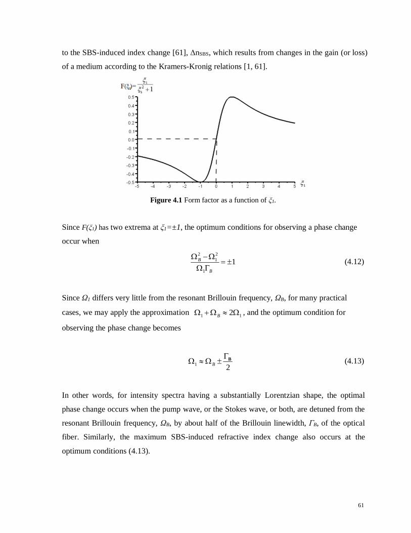
61
to the SBS-induced index change [61], ΔnSBS, which results from changes in the gain (or loss)
of a medium according to the Kramers-Kronig relations [1, 61].
Figure 4.1 Form factor as a function of ξ1.
Since F(ξ1) has two extrema at ξ1=±1, the optimum conditions for observing a phase change
occur when
11
21
2
B
B (4.12)
Since Ω1 differs very little from the resonant Brillouin frequency, ΩB, for many practical
cases, we may apply the approximation 11 2 B , and the optimum condition for
observing the phase change becomes
21B B (4.13)
In other words, for intensity spectra having a substantially Lorentzian shape, the optimal
phase change occurs when the pump wave, or the Stokes wave, or both, are detuned from the
resonant Brillouin frequency, ΩB, by about half of the Brillouin linewidth, ΓB, of the optical
fiber. Similarly, the maximum SBS-induced refractive index change also occurs at the
optimum conditions (4.13).
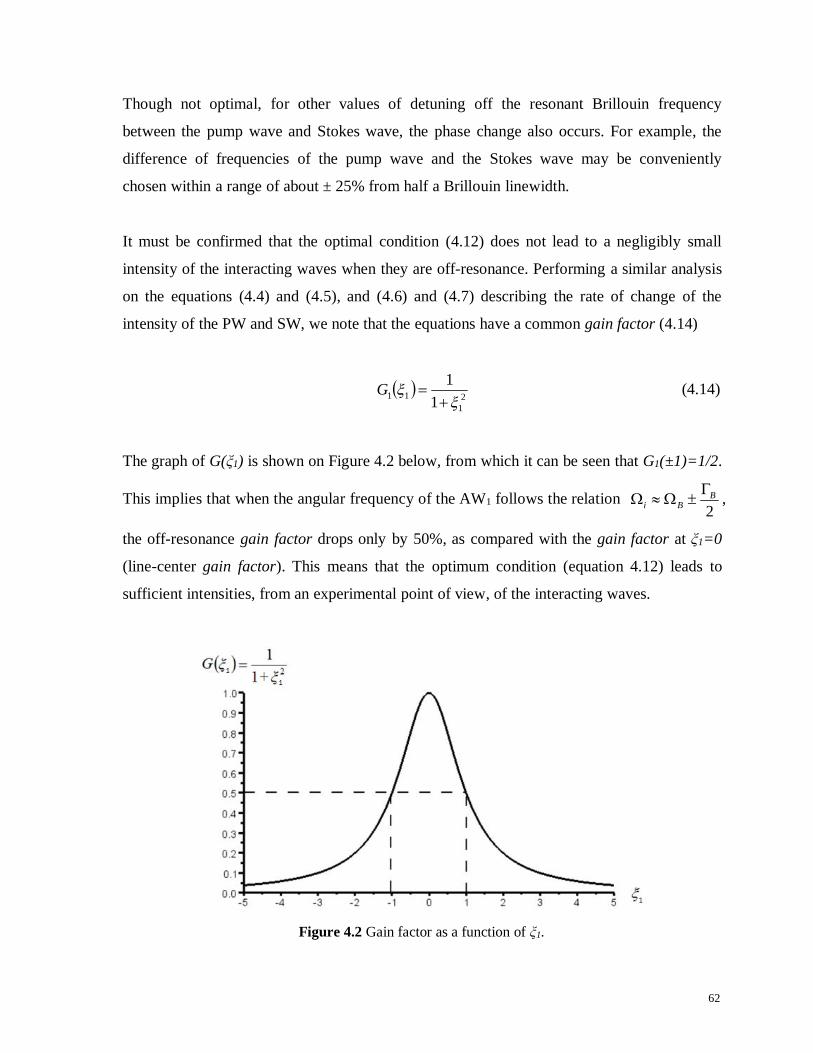
62
Though not optimal, for other values of detuning off the resonant Brillouin frequency
between the pump wave and Stokes wave, the phase change also occurs. For example, the
difference of frequencies of the pump wave and the Stokes wave may be conveniently
chosen within a range of about ± 25% from half a Brillouin linewidth.
It must be confirmed that the optimal condition (4.12) does not lead to a negligibly small
intensity of the interacting waves when they are off-resonance. Performing a similar analysis
on the equations (4.4) and (4.5), and (4.6) and (4.7) describing the rate of change of the
intensity of the PW and SW, we note that the equations have a common gain factor (4.14)
21
11 11
G (4.14)
The graph of G(ξ1) is shown on Figure 4.2 below, from which it can be seen that G1(±1)=1/2.
This implies that when the angular frequency of the AW1 follows the relation2B
Bi
,
the off-resonance gain factor drops only by 50%, as compared with the gain factor at ξ1=0
(line-center gain factor). This means that the optimum condition (equation 4.12) leads to
sufficient intensities, from an experimental point of view, of the interacting waves.
Figure 4.2 Gain factor as a function of ξ1.

63
From observation of Figure 4.1, it may be concluded that
F(0)=0 (4.15)
For which we have β5=β7=0, and therefore
0
zi when Ω1=ΩB, i=1,2. (4.16)
In other words, at the resonant Brillouin frequency, the phases of the pump wave and the
Stokes wave remain constant at every point in the fiber.
Likewise, off-resonance, i.e. When Ω1≠ΩB, we have
|F(ξ1)|>0 (4.17)
For which we have β5, β7 >0. Therefore,
0
zi , i=1,2. (4.18)
In other words, the phases of the pump wave and Stokes wave change along the fiber if
Ω1≠ΩB i.e detuned from the resonant Brillouin frequency.
4.3 Proposed Experimental Setup
To demonstrate the proposed theory of section 4.2, an experimental setup is proposed, which
is shown in Figure 4.3.

64
Figure 4.3 Experimental setup.
The experimental setup is comprised of a SW laser source, a beamsplitter, a pump laser
source, an electronic variable optical attenuator (eVOA), which is used as a source of
amplitude modulation, an active Brillouin scattering optical fiber, a path equalizing optical
fiber, a first and second reflective mirror, a semi-transparent mirror, a screen with tiny
aperture, and a photodiode.
The experimental setup of Figure 4.3 operates as follows. The pump laser source, for
example, a tunable laser source, generates a pump wave, which passes through the eVOA.
The resulting wave is an amplitude modulated pump wave, which is injected into one end of
the active optical fiber. The SW laser source, for example a tunable laser source, generates a
Stokes wave which encounters the beamsplitter, and is split into an incident Stokes wave and
a reference optical signal. The incident Stokes wave is injected into the opposite end of the
active optical fiber, such that the incident Stokes wave and the amplitude modulated pump
wave counter-propagate in the active optical fiber, causing the phase of the incident Stokes
wave to change according to the equation (4.7).
For clarity of the experimental setup of Figure 4.3, the second reflective mirror is
schematically shown as spatially separated from the pump wave. In practice, the second
reflective mirror is replaced with a second semi-transparent mirror.
In accordance with the theory recommendations in the section 4.2 above, the frequency of
the Stokes wave is detuned from the resonant Brillouin frequency to create conditions

65
necessary for the phases of the amplitude modulated pump wave and the incident Stokes
wave to change. Preferably, the frequency of the Stokes wave is chosen to satisfy the optimal
conditions as described in equation (4.13) above, to induce a maximum phase change,
thereby making it easier to measure. An output Stokes wave, with the phase changed in
accordance with the chosen attenuation of the eVOA, is reflected off the second reflective
mirror, at about a 90° angle, creating a phase modulated Stokes beam.
The first reference optical signal is reflected at about a 90° angle off a first reflective mirror,
to create a second reference optical signal, which is passed through a path equalizing optical
fiber that is substantially identical to the active Brillouin scattering optical fiber in all
respects. The result is an output reference beam which exits the path equalizing optical fiber,
the purpose of which is to equalize the optical path for the first reference optical signal with
the optical path of the incident Stokes wave, keeping both mutually coherent. Since the
typical coherence length of a typical laser, such as an He-Ne laser, is around 20 cm, the
difference in optical paths between the active Brillouin Scattering optical fiber and the path
equalizing optical fiber should be much smaller than 20 cm, preferably not exceeding several
centimeters.
The output reference beam passes through a semi-transparent mirror, while the phase
modulated Stokes beam is reflected from the semi-transparent mirror, such that both the
output reference beam and the phase modulated Stokes beam converge to create an
interference pattern on the screen with tiny aperture. The angle of convergence is selected to
be small enough (preferably substantially smaller than 1`) to widen the interference pattern,
such as a 10 mm wide interference pattern. The required convergence angle can be estimated
from the expression 2d·sin(ϑ)=λ, where λ is the wavelength, d is the width of the interference
patterns, and 2ϑ is the convergence angle between the phase modulated Stokes beam and the
output reference beam.
When the interference pattern becomes visible, the convergence angle can be adjusted
experimentally as required. To maintain the stability of the interference pattern for the
amount of time required for measurements (presumably ~ 5-10 min), the entire setup is

66
preferably mounted on an anti-vibrational table or breadboard, such as produced by Newport
Corporation.
The aperture on the screen with tiny aperture is chosen to be much smaller in diameter than
the width of the light and dark bands of the interference pattern, which permits the light from
the interference pattern to be detected by the photodiode. Initially, the aperture is adjusted to
occupy a position of an interference pattern at about a middle point between a light and a
dark band of the interference pattern, which provides for a substantially linear region of
intensity variation. When the eVOA is controlled to a different attenuation from the initial
attenuation, the phase of the output Stokes wave is expected to change relative to the phase
of the output reference beam, causing the light and dark bands of the interference pattern to
change locations relative to the aperture in the transverse direction. Therefore, the amount of
light that reaches the photodiode changes approximately proportionally to the phase shift,
allowing the phase shift to be measured.
A controllable change of attenuation of the eVOA allows for the measurement of the phase
shift versus the intensity of the amplitude modulated pump wave. Simulation results are
shown in Table 4.1 below.
Table 4.1 Simulation results for the experimental setup
Parameters of the Fiber Detuning Phase Change of SW (rad)
γe=0.902ω1=8.381097∙105 GHzω2= 8.380691∙105 GHzΩ1=4.053668∙101 GHzΩB=4.053668∙101 GHz
n=1.45, c= 299792.458 km/sv=5000 m/s, ρ0=2.21 g/cm3
ΓB = 0.1 GHz, L=1000 mPW power: PPW=10mWSW power: PSW=9mW
B 5.01 B
(optimal conditions)~1.2
B 25.01 B ~0.2
B 1.01 B ~0.08

67
As can be seen from Table 4.1, the phase change of the output Stokes wave is sufficiently
large and suitable for conducting measurements. It has also been noticed that, when the pump
wave is amplitude modulated, the phase change of the output Stokes wave is larger for pump
waves experiencing larger depletion, for example, when the depletion of the pump wave is
larger than about 50%.
Also, the Stokes wave can be amplitude modulated instead of the pump wave, thus causing a
phase modulation of the pump wave.
4.4 Optical phase modulator construction
An optical phase modulator based on the principles outlined in Sections 4.2 and 4.3 is shown
in Figure 4.4 below. It comprises an active Brillouin scattering optical fiber, a pump and SW
laser source, for example tunable laser sources, an eVOA, and a reflective mirror.
Figure 4.4 Optical phase modulator construction.
For clarity of the setup of Figure 4.4, the reflective mirror is schematically shown being
spatially separated from an amplitude modulated pump wave. In practice, the reflective
mirror is replaced with a semi-transparent mirror.
In Figure 4.4, the pump laser source generates a pump wave, the amplitude of which is
modulated by a low frequency signal (for example speech signal, which is not shown) using
the amplitude modulator, such as an eVOA. The resulting amplitude modulated pump wave
is injected into one end of the active optical fiber. A Stokes wave is generated by the SW
laser source, that is injected into the opposite end of the active optical fiber, such that the two
waves counter-propagate in the active optical fiber. The SW laser source is used to detune
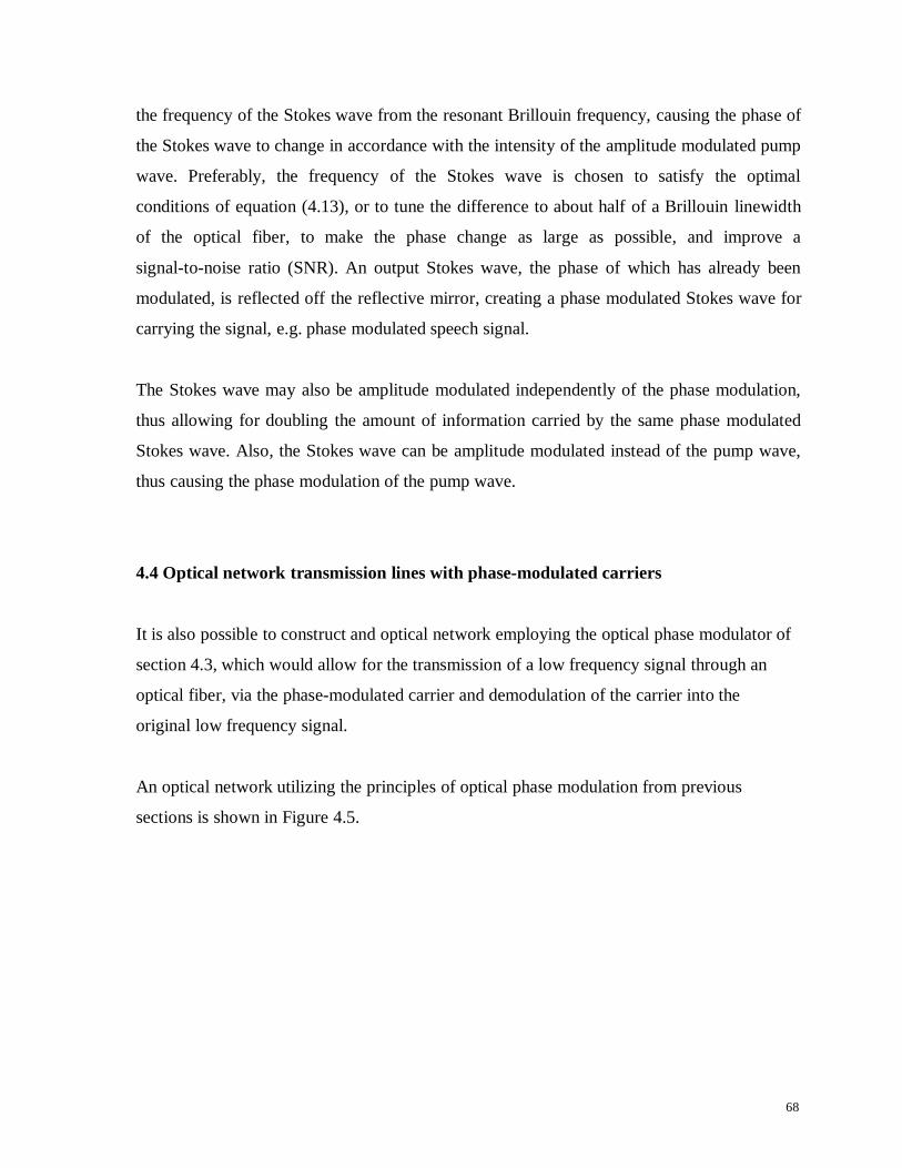
68
the frequency of the Stokes wave from the resonant Brillouin frequency, causing the phase of
the Stokes wave to change in accordance with the intensity of the amplitude modulated pump
wave. Preferably, the frequency of the Stokes wave is chosen to satisfy the optimal
conditions of equation (4.13), or to tune the difference to about half of a Brillouin linewidth
of the optical fiber, to make the phase change as large as possible, and improve a
signal-to-noise ratio (SNR). An output Stokes wave, the phase of which has already been
modulated, is reflected off the reflective mirror, creating a phase modulated Stokes wave for
carrying the signal, e.g. phase modulated speech signal.
The Stokes wave may also be amplitude modulated independently of the phase modulation,
thus allowing for doubling the amount of information carried by the same phase modulated
Stokes wave. Also, the Stokes wave can be amplitude modulated instead of the pump wave,
thus causing the phase modulation of the pump wave.
4.4 Optical network transmission lines with phase-modulated carriers
It is also possible to construct and optical network employing the optical phase modulator of
section 4.3, which would allow for the transmission of a low frequency signal through an
optical fiber, via the phase-modulated carrier and demodulation of the carrier into the
original low frequency signal.
An optical network utilizing the principles of optical phase modulation from previous
sections is shown in Figure 4.5.
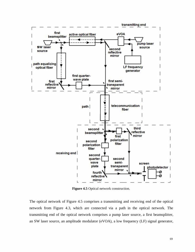
69
Figure 4.5 Optical network construction.
The optical network of Figure 4.5 comprises a transmitting and receiving end of the optical
network from Figure 4.3, which are connected via a path in the optical network. The
transmitting end of the optical network comprises a pump laser source, a first beamsplitter,
an SW laser source, an amplitude modulator (eVOA), a low frequency (LF) signal generator,

70
an active Brillouin scattering optical fiber, a passive path equalizing optical fiber, a first and
second reflective mirror, a first quarter-wave plate, and a first semi-transparent mirror.
The receiving end of the optical network comprises a second beamsplitter, a first and second
polarization filter, a second quarter-wave plate, a third and fourth reflective mirror, a second
semi-transparent mirror, a screen with a pinhole, and a photodetector.
The path in the optical network comprises a telecommunication fiber acting as a transmission
channel.
The pump laser source generates a pump wave, which may also be referred to as a first
optical signal. The first beamsplitter acts to split the pump wave into a pump wave to be
phase modulated and a reference optical signal, both with parallel polarization.
The SW laser source generates a Stokes wave, which may also be referred to as a second
optical signal. The Stokes wave and a low frequency signal, which is generated by the low
frequency signal generator, are sent to the amplitude modulator which generates an
amplitude-modulated wave, or AM carrier. The AM carrier is injected into one end of the
active optical fiber, while the pump wave to be phase modulated is injected into an opposite
end of the active optical fiber. The pump wave to be phase modulated and the AM carrier
counter-propagate inside the active Brillouin scattering optical fiber, resulting in
transforming the pump wave to be phase modulated into a phase modulated pump wave, also
with parallel polarization.
For clarity of the setup of Figure 4.5, the first reflective mirror is schematically shown as
spatially separated from a AM carrier. In practice, the first reflective mirrors replaced with a
third semi-transparent mirror.
The phase modulated pump wave is reflected off the first reflective mirror, at about a 90°
angle, creating a phase modulated optical signal. Likewise, the reference optical signal enters
the passive path equalizing optical fiber, which acts as an optical path equalizer, and is then
71
reflected off the second reflective mirror at about a 90° angle, creating a reference wave. The
reference wave passes through the first quarter-wave plate, which changes its polarization to
a perpendicular polarization, resulting in a first perpendicular polarized reference beam. The
first perpendicular polarized reference beam is perpendicularly polarized, while the phase
modulated optical signal is still parallel polarized.
The phase modulated optical signal passes through the first semi-transparent mirror, resulting
in a polarization perpendicular reference beam, while the first perpendicular polarized
reference beam is reflected, at about a 90° angle, resulting in a polarization parallel phase
modulated beam. Both the polarization perpendicular reference beam and the polarization
parallel phase modulated beam, which in Figure 4.5 are drawn separate from each other only
for the purpose of clarity, enter the telecommunication fiber. Upon exiting the
telecommunication fiber, the polarization perpendicular reference beam becomes a
destination reference beam, and the polarization parallel phase modulated beam becomes a
destination phase modulated beam. Both the destination reference beam and the destination
phase modulated beam encounter the second beamsplitter, which redirects them to the first
and second polarization filters.
The first polarization filter allows only the destination phase modulated beam to pass through,
to be reflected off the third reflective mirror, as well as the second semi-transparent mirror,
to produce a converging phase modulated beam. The polarization filter allows only the
destination reference beam to pass through, creating a second perpendicular polarized
reference beam. The resulting second perpendicular polarized reference beam passes through
the second quarter-wave plate, which is polarization to parallel, resulting in a first parallel
polarized reference beam. The first parallel polarized reference beam is reflected off the
fourth reflective mirror, and passes through the second semi-transparent mirror, producing a
converging reference beam.
The resulting converging phase modulated beam and the converging reference beam, both
with the same polarization, converge at a small angle (preferably smaller than 1`), and
overlap on a screen with a pinhole. The light passing through is detected by the photodetector.

72
When the phase of the converging phase modulated beam changes (due to the phase
modulation) relative to the phase of the converging reference beam, the interference pattern,
of variable intensity, shifts in the transverse direction approximately proportionally to the
change in phase. As a result, the intensity of light which passes through the screen with a
pinhole also changes respectively. In this way, the low frequency signal is decoded from the
converging phase modulated beam. Consequently, we were able to transmit the low
frequency signal through an optical network to its destination and restore it at this
destination.
It is also possible to amplitude modulate the pump wave with the amplitude modulator,
independently of the phase modulation, and as mentioned in previous sections, the pump
wave may also be amplitude modulated instead of the Stokes wave, thus causing the phase
modulation of the Stokes wave.
Finally, instead of using two differently polarized beams: the phase modulated optical signal
and the first perpendicular polarized reference beam, propagating through the same
telecommunication fiber, two separate fibers with substantially similar characteristics could
be used so that one fiber propagates the phase modulated optical signal, while another fiber
propagates the first perpendicular polarized reference beam. In this case, both the phase
modulated optical signal and the first perpendicular polarized reference beam may have
similar polarizations, and the second quarter-wave plate will not be needed for producing the
interference pattern.
4.5 Summary
Therefore, an improved method of phase-modulation, based on the principles of stimulated
Brillouin scattering, has been proposed, as well as an optical phase network employing the
same.

73
Chapter 5
Polarization Effects in SBS
5.1 Introduction
As described in section 1.4, this chapter will introduce several important applications of
birefringence in optical fibers, relating to telecommunications and fiber sensing. The effect
of the spectral shift due to increased birefringence is investigated, as well as spectral
distortion due to various degrees of birefringence will be investigated for steady-state and
transient pulsed regimes. Namely, the steady-state model presented for linearly polarized (LP)
light will be shown to be a valuable measure of the experimentally realistic case of non-ideal
LP light in optical fibers. The degree of spectral distortion may be used as an indication of
the quality of linear polarization during the SBS interaction, or as a measure of power
leaking between the fast and slow modes. Furthermore, increased power leaking between the
fast and slow modes for LP can be used to create a regime that is more favourable for sensing
applications related to SBS. In the pulsed regime, spectral broadening and depletion of the
Stokes spectrum will be observed as a result of increased birefringence. Spectral distortion is
detrimental for fiber sensing and telecommunications, hence methods of minimizing this
effect are important to investigate.
Additionally, the effects of various elliptical polarizations on output spectral shape will be
investigated for the steady-state model, including spectral spreading effects and spectral
broadening. Methods of maintaining a pulse fidelity and full width at half maximum
(FWHM), as compared to non-polarized light in a non-birefringent fiber, will be proposed.
In this chapter, the most comprehensive SBS equations are presented, considering the
birefringence effects in optical fibers. Besides the usual slowly varying amplitude
approximation, the only extra approximation of the model is the assumption that the phonon
fields are established almost instantaneously, namely, the time it takes for the acoustic
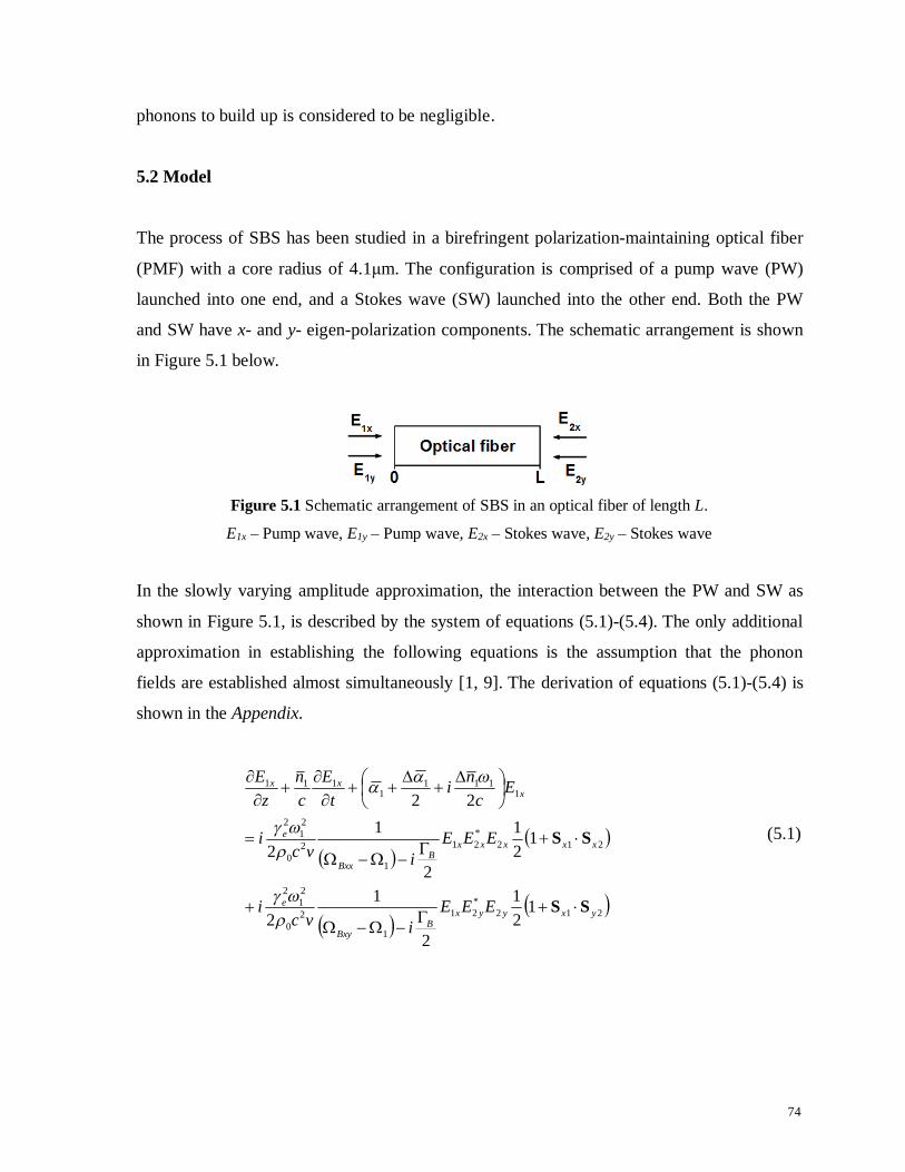
74
phonons to build up is considered to be negligible.
5.2 Model
The process of SBS has been studied in a birefringent polarization-maintaining optical fiber
(PMF) with a core radius of 4.1μm. The configuration is comprised of a pump wave (PW)
launched into one end, and a Stokes wave (SW) launched into the other end. Both the PW
and SW have x- and y- eigen-polarization components. The schematic arrangement is shown
in Figure 5.1 below.
Figure 5.1 Schematic arrangement of SBS in an optical fiber of length L.
E1x – Pump wave, E1y – Pump wave, E2x – Stokes wave, E2y – Stokes wave
In the slowly varying amplitude approximation, the interaction between the PW and SW as
shown in Figure 5.1, is described by the system of equations (5.1)-(5.4). The only additional
approximation in establishing the following equations is the assumption that the phonon
fields are established almost simultaneously [1, 9]. The derivation of equations (5.1)-(5.4) is
shown in the Appendix.
212
*21
1
20
21
2
212*21
1
20
21
2
1111
1111
121
2
12
121
2
12
22
yxyyxB
Bxy
e
xxxxxB
Bxx
e
xxx
EEEivc
i
EEEivc
i
Ec
nit
Ecn
zE
SS
SS
(5.1)
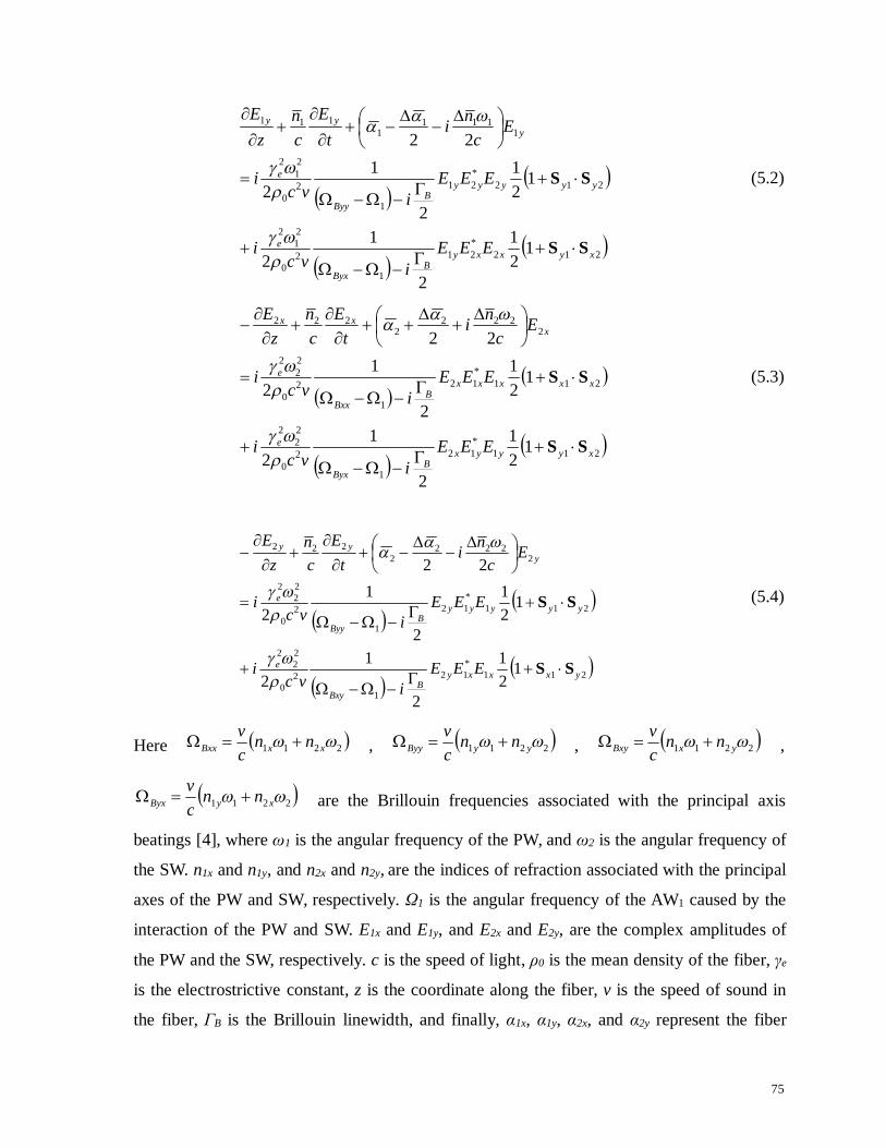
75
212
*21
1
20
21
2
212*21
1
20
21
2
1111
1111
121
2
12
121
2
12
22
xyxxyB
Byx
e
yyyyyB
Byy
e
yyy
EEEivc
i
EEEivc
i
Ec
nit
Ecn
zE
SS
SS
(5.2)
211
*12
1
20
22
2
211*12
1
20
22
2
2222
2222
121
2
12
121
2
12
22
xyyyxB
Byx
e
xxxxxB
Bxx
e
xxx
EEEivc
i
EEEivc
i
Ec
nit
Ecn
zE
SS
SS
(5.3)
211
*12
1
20
22
2
211*12
1
20
22
2
2222
2222
121
2
12
121
2
12
22
yxxxyB
Bxy
e
yyyyyB
Byy
e
yyy
EEEivc
i
EEEivc
i
Ec
nit
Ecn
zE
SS
SS
(5.4)
Here 2211 xxBxx nncv , 2211 yyByy nn
cv , 2211 yxBxy nn
cv ,
2211 xyByx nncv
are the Brillouin frequencies associated with the principal axis
beatings [4], where ω1 is the angular frequency of the PW, and ω2 is the angular frequency of
the SW. n1x and n1y, and n2x and n2y, are the indices of refraction associated with the principal
axes of the PW and SW, respectively. Ω1 is the angular frequency of the AW1 caused by the
interaction of the PW and SW. E1x and E1y, and E2x and E2y, are the complex amplitudes of
the PW and the SW, respectively. c is the speed of light, ρ0 is the mean density of the fiber, γe
is the electrostrictive constant, z is the coordinate along the fiber, v is the speed of sound in
the fiber, ΓB is the Brillouin linewidth, and finally, α1x, α1y, α2x, and α2y represent the fiber

76
attenuations of the principal axes of polarization of the two interacting waves.
The S1x, S1y, S2x, and S2y represent the Stokes vectors in the Poincaré sphere polarization
representation [68, 69], and are used to define the polarization of the propagating lights [61,
68]. Some extra relations of importance are the following: Sx1 = -Sy1 for forward propagating
light (PW), and Sx2 = -Sy2 for backward propagating light (SW). Furthermore, it is
worthwhile to emphasize that in the above system of equations (5.1)-(5.4), Sx1 describes the
principal state of polarization vector for the forward propagating light, and Sx2 describes the
principal state of the polarization vector of the backward propagating light. In this case, if Sx1
is defined as Sx1 = (a, b, c), then it must follow that Sy1 = (-a, -b, -c), and neglecting the
dispersion effect, then Sx2 = (a, b, -c) and Sy2 = (-a, -b, c), where a, b and c are the Stokes
vector components, the third component, c, describing circular birefringence, and are
normalized such that a2 + b2 + c2 = 1. From this arrangement it is apparent that for fibers
having elliptical birefringence (0 < |c| < 1), the most general beating situation will be excited,
i.e. there will exist four acoustic resonances.
Lastly, some remaining simplifications were introduced to the system of equations (5.1)-(5.4)
to make the birefringence effect more explicit. This can be justified by the fact that
birefringence and polarization dependent loss are both small. It is defined 211
1yx nn
n
,
yx nnn 111 , 222
2yx nn
n
, yx nnn 222 , and 211
1yx
, yx 111 ,
222
2yx
, yx 222 .
In the above arrangement, the PW input parameters are known only at the beginning of the
fiber, i.e. at z=0. Correspondingly, the SW input parameters are known only at the end of the
fiber, i.e. at z=L, where L is the length of the fiber. Therefore, the boundary conditions for the
system of equations (5.1)-(5.4) are similar to previously-studied configurations with one
pulse [4, 65]. The conditions for two pulses are as follows:
|E1x(0)|2 = E21x0 ; |E1y(0)|2 =E21y0 ; |E2x(L)|2 = E22x0; |E2y(L)|2 = E22y0; (5.5)
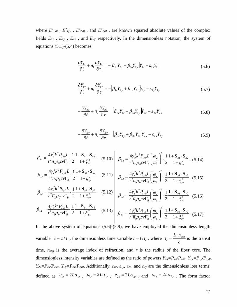
77
where E21x0 , E21y0 , E22x0 , and E22y0 , are known squared absolute values of the complex
fields E1x , E1y , E2x , and E2y respectively. In the dimensionless notation, the system of
equations (5.1)-(5.4) becomes
xxxybxaxx YYYYYnY
11121211
11
(5.6)
yyyxdycyy YYYY
Yn
Y1112121
11
1
(5.7)
xxxybxaxx YYYYYnY
22213132
22
(5.8)
yyyxdycyy YYYY
Yn
Y2221313
22
2
(5.9)
221
022
0222
1 11
214
xx
xx
B
xea cvnr
LPk
SS
(5.10)
2y2x1
022
0222
1 11
214
xyB
yeb cvnr
LPk
SS(5.11)
2y2y1
022
0222
1 11
214
yyB
yec cvnr
LPk
SS(5.12)
221
022
0222
1 11
214
yx
xy
B
xed cvnr
LPk
SS(5.13)
221
2
1
2
012
0122
3 11
214
xx
xx
B
xea cvnr
LPk
SS
(5.14)
221
2
1
2
012
0122
3 11
214
yx
xy
B
yeb cvnr
LPk
SS
(5.15)
221
2
1
2
012
0122
3 11
214
yy
yy
B
yec cvnr
LPk
SS
(5.16)
221
2
1
2
012
0122
3 11
214
xy
yx
B
xed cvnr
LPk
SS
(5.17)
In the above system of equations (5.6)-(5.9), we have employed the dimensionless length
variable Lz / , the dimensionless time variable ctt / , wherecnL
t avgc
is the transit
time, navg is the average index of refraction, and r is the radius of the fiber core. The
dimensionless intensity variables are defined as the ratio of powers Y1x=P1x/P1x0, Y1y=P1y/P1y0,
Y2x=P2x/P2x0, Y2y=P2y/P2y0. Additionally, ε1x, ε1y, ε2x, and ε2y are the dimensionless loss terms,
defined as xx L 11 2 , yy L 11 2 , xx L 22 2 , and yy L 22 2 . The form factor

78
component of the β-coefficients is defined as
2
1
B
Bijij
, where i=x,y, and j=x,y. The
Method of Characteristics was employed [61, 75, 76, 77] and the following change of
variables was performed, where the approximation nnn 21 was used.
n
u 1(5.18)
nv 1
(5.19)
The resulting system of equations is as follows, with β-coefficients as defined in expressions
(5.10)-(5.17).
xxxybxax YYYY
dudY
11121211 (5.20)
yyyxdycy YYYY
dudY
11121211 (5.21)
xxxybxax YYYY
dvdY
22213132 (5.22)
yyyxdycy YYYY
dvdY
22213132 (5.23)
The change of variables u and v transforms the system of equations (5.6)-(5.9) of counter-
propagating waves into the system of equations (5.20)-(5.23) of co-propagating waves.
Consequently, we are able to set the following initial conditions
1tanhtanh0, 22110 btabtatYij (5.24)
both of which take place at the same end of the new coordinate system, where i=1,2, and
j=x,y. The parameters a1 and a2 determine the rise time of the PW and SW pulse profiles,
while the parameters b1 and b2 define the center of the pulses via the expression |b2-b1|/2.
Though there exist many numerical methods of solution for SBS equations [75, 78, 79, 80,

79
81, 82, 83], the fourth order Runge-Kutta method (RK4) was used to numerically solve the
system of equations (5.20)-(5.23), and was chosen for its stability and relatively large step
size. Details of this numerical method of solution are summarized in the Appendix.
5.3. Results and Discussion
Output spectra were calculated by detuning the Stokes frequency, ω2. Output powers were
calculated as P1x-out = P1x0 ∙Y1x-out, P1y-out = P1y0 ∙Y1y-out, P2x-out = P2x0 ∙Y2x-out, and P2y-out = P2y0
∙Y2y-out, and the total power of the pump and Stokes waves was calculated to be P1 = P1x + P1y
and P2 = P2x + P2y respectively. Also, the attenuation in the fiber has been approximated as
α1x=α1y=α2x=α2y=α=0.2 dB/km, and the following parameters of the fiber were used:
navg=1.45, γe=0.902, λ=1550nm, ρ0=2.21g/cm3, v=5616m/s, ΓB=0.1GHz.
5.3.1 Spectral Shift
The appearance of a fast and slow axis results in two optical modes in the fiber with different
SBS frequency shifts, causing a mismatch in the corresponding momentum vectors of the
acoustic waves, thereby making it impossible for both principal axes to be resonant with the
acoustic phonons in the conventional sense. The mismatch in phonon resonance causes a
Brillouin shift, ΔυB, and the larger the birefringence, the larger the Brillouin shift.
Figure 5.2 below shows the magnitude of the Brillouin shift in the output PW and SW
spectra.
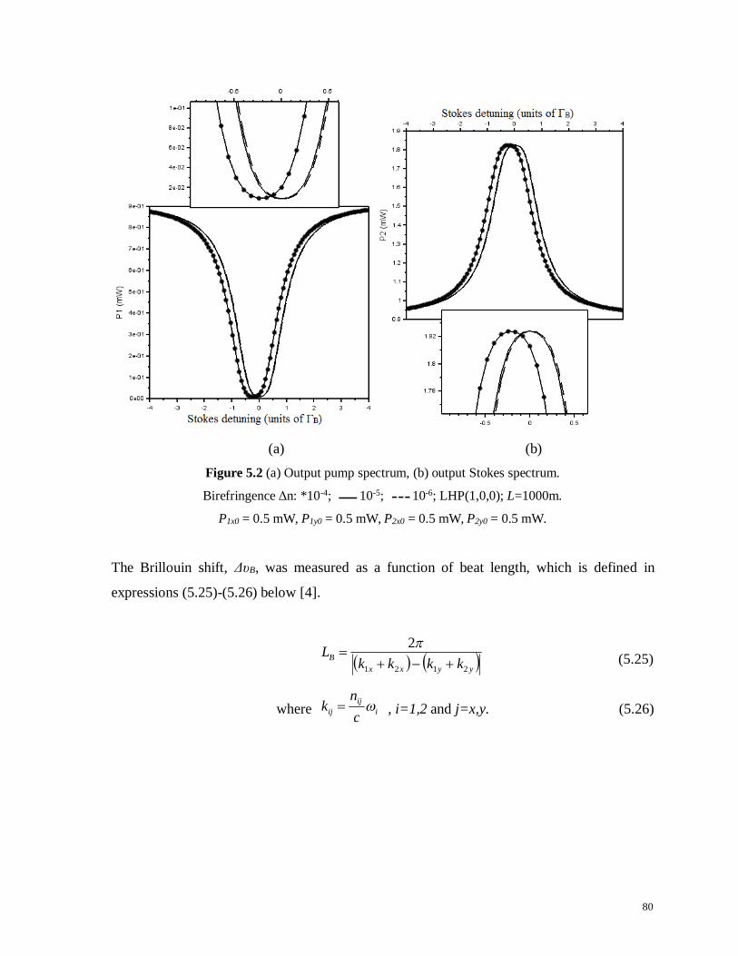
80
(a) (b)Figure 5.2 (a) Output pump spectrum, (b) output Stokes spectrum.
Birefringence Δn: *10-4; 10-5; 10-6; LHP(1,0,0); L=1000m.
P1x0 = 0.5 mW, P1y0 = 0.5 mW, P2x0 = 0.5 mW, P2y0 = 0.5 mW.
The Brillouin shift, ΔυB, was measured as a function of beat length, which is defined in
expressions (5.25)-(5.26) below [4].
yyxxB kkkk
L2121
2
(5.25)
where iij
ij cn
k , i=1,2 and j=x,y. (5.26)
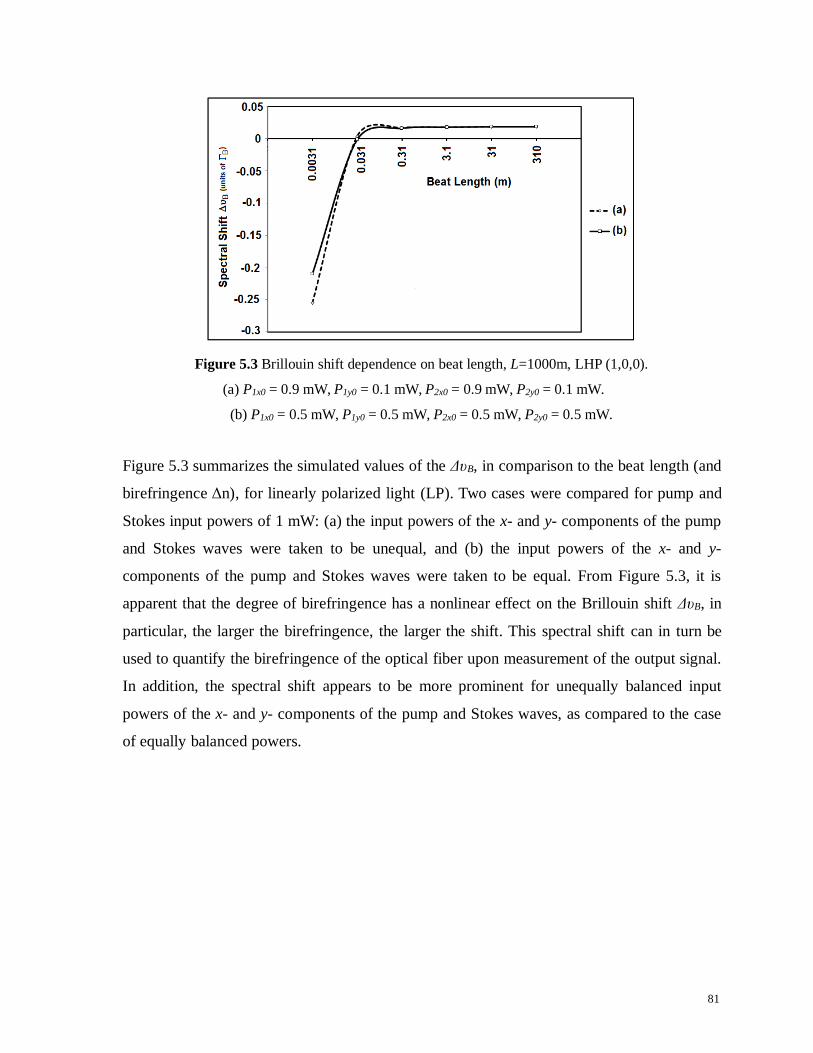
81
Figure 5.3 Brillouin shift dependence on beat length, L=1000m, LHP (1,0,0).
(a) P1x0 = 0.9 mW, P1y0 = 0.1 mW, P2x0 = 0.9 mW, P2y0 = 0.1 mW.
(b) P1x0 = 0.5 mW, P1y0 = 0.5 mW, P2x0 = 0.5 mW, P2y0 = 0.5 mW.
Figure 5.3 summarizes the simulated values of the ΔυB, in comparison to the beat length (and
birefringence Δn), for linearly polarized light (LP). Two cases were compared for pump and
Stokes input powers of 1 mW: (a) the input powers of the x- and y- components of the pump
and Stokes waves were taken to be unequal, and (b) the input powers of the x- and y-
components of the pump and Stokes waves were taken to be equal. From Figure 5.3, it is
apparent that the degree of birefringence has a nonlinear effect on the Brillouin shift ΔυB, in
particular, the larger the birefringence, the larger the shift. This spectral shift can in turn be
used to quantify the birefringence of the optical fiber upon measurement of the output signal.
In addition, the spectral shift appears to be more prominent for unequally balanced input
powers of the x- and y- components of the pump and Stokes waves, as compared to the case
of equally balanced powers.
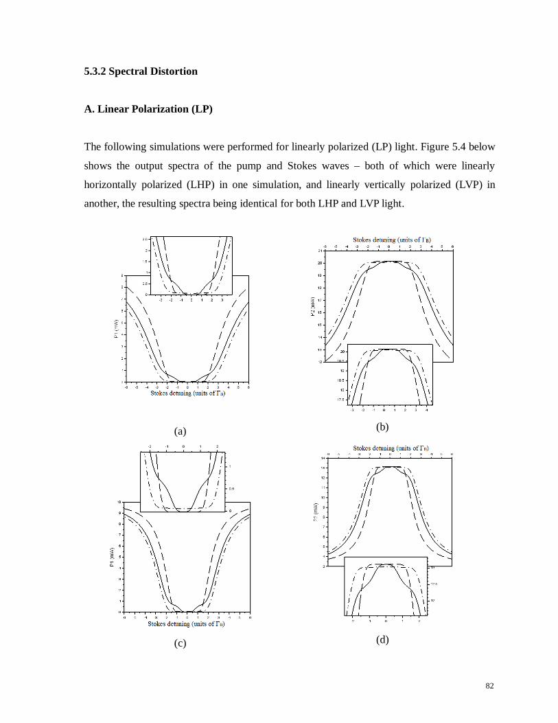
82
5.3.2 Spectral Distortion
A. Linear Polarization (LP)
The following simulations were performed for linearly polarized (LP) light. Figure 5.4 below
shows the output spectra of the pump and Stokes waves – both of which were linearly
horizontally polarized (LHP) in one simulation, and linearly vertically polarized (LVP) in
another, the resulting spectra being identical for both LHP and LVP light.
(a) (b)
(c) (d)

83
(e) (f)
Figure 5.4 Left: output pump spectrum; Right: output Stokes spectrum.
(a)-(b) steady-state; (c)-(d) 240ns pulse; (e)-(f) 79ns pulse; Birefringence Δn=10-4; L=1 km.
: P1x0 = 10.0 mW, P1y0 = 1.0 mW, P2x0 = 10.0 mW, P2y0 = 1.0 mW; LHP (1,0,0);
: P1x0 = 10.9 mW, P1y0 = 0.1 mW, P2x0 = 10.9 mW, P2y0 = 0.1 mW; LHP (1,0,0);
: P1x0 = 10.0 mW, P1y0 = 1.0 mW, P2x0 = 10.0 mW, P2y0 = 1.0 mW; no pol (0,0,0).
It is often experimentally not possible to achieve a 100% separation of power between the
slow and fast modes of the signal. There is power leakage between the x- and y-axes [84],
especially when additional optical components, such a polarization controllers or scramblers
[85, 86], are used. Hence, for a 11 mW signal, it is a realistic assumption that as much as 1
mW of power could be present in the vertical mode of the signals for LHP light. Likewise,
for LVP lights, it is also experimentally plausible to have as much as 1 mW of power in the
horizontal mode.
The shape of the output spectra in Figures 5.4 can be explained by the modified interaction
between the pump and Stokes waves during LP. Referring to the system of equations (5.20)-
(5.23) and β-coefficients (5.10)-(5.17), we see that the β-coefficients β1b, β1d, β3b and β3d are
reduced to zero for both LHP and LVP light. As a result, the system of equations (5.20)-(5.23)
is broken up into two smaller systems consisting of equations: a) (5.20) and (5.21), and b)

84
(5.22) and (5.23) respectively, which are independent of each other. The first system
describes the interaction between the horizontal components (x-components) of the pump
and Stokes waves, and the second system describes the interaction between the vertical
components (y-components) of the pump and Stokes waves. In other words, interactions
along the x- and y-components become independent from each other, which is to be expected
during linear polarization.
In Figure 5.4, which represents the output pump and Stokes spectra of LHP light, the little
'blip' at the bottom/top of the spectra is the y-component contribution, while the 'general'
shape of the spectra is a result of the x-component contribution. Since the power in the
horizontal mode is large for LHP light, the resultant depletion of the PW and amplification of
the SW are also large, leading to the general trend of the output spectra in Figure 5.4. This is
the spectral shape which would be expected for an idealized LHP light (or perhaps light with
no consideration for polarization at all). However, the LHP is not ideal, and there exists a
small interaction in the vertical component. Since the power along the y-axis is small, the
resultant contribution is also small. As can be seen from Figure 5.4, the smaller the power in
the y-component, the smaller the contribution, and the weaker the spectral distortion of the
graph. In other words, increasing powers in the y-components have been chosen to
demonstrate the increasing degree of spectral distortion. For P1y=P2y=1mW, the spectral
'blip' is much larger than for the case where P1y=P2y=0.1mW. However, while a small power
leakage causes a smaller spectral distortion or 'blip', it yields an output spectra with a larger
depletion, or 'flat-top', than in the case of larger power leakage. For the steady-state regime,
shown in Figures 5.4(a)-(b), where both the pump and Stokes waves are continuous waves,
the 'flat-top' effect is more prominent and the spectral 'blip' is less pronounced, as compared
to shorter pulse lengths of 240ns and 79ns, shown in Figures 5.4(c)-(d) and 5.4(e)-(f)
respectively. With decreasing temporal pulse width, the power leakage causes the distorted
spectral tip to be sharper and more pronounced, as compared to longer pulses.
For sensing applications, it is detrimental to have a depleted spectrum [70, 71, 72], since
depletion and spectral flattening makes it difficult to accurately measure the center frequency
of the spectrum. Although the distorted spectra with smaller depletion, obtained from the

85
steady-state interaction of the PW and SW, may not have a sufficiently prominent spectral tip
for sensing applications, it is an improvement none-the-less, as compared to the case of
larger depletion, where the 'flat-top' spans an even larger frequency range.
As shown in Figure 5.4(e)-(f), a shorter pulse length of 79ns undergoing spectral leakage
between the fast and slow modes has a sufficiently prominent spectral tip for measurement in
sensing applications. As such, by using the distortion effects caused by birefringence to our
advantage, it is possible to provide a regime that is favourable for sensing applications
related to SBS, by increasing the power leakage between the fast and slow modes, as well as
decreasing the pulse length during LP.
In the case of LVP, also shown in Figure 5.4, the roles of the x- and y-components are
reversed, but the interaction is identical. For this reason, the two cases of LHP and LVP light,
shown in Figures 5.4, give identical results, since in either case, the interaction along the
slow or fast axes remains the same.
Also shown in the Figure 5.4, the output spectra of LP light is shown in comparison to light
without a dependence on polarization – namely light having a Stokes vector S=(0,0,0), which
has been taken to be a first-order approximation to truly unpolarized light. The spectra of the
LP is spread out in the frequency domain, as compared to non-polarized light. This effect can
be explained by the nature of the LP interaction between the pump and Stokes waves. As
discussed above, when LP is not ideal, there exists a small independent interaction along
either the fast or slow mode, contributing to the spectral distortion. The interaction along the
main axis of polarization, however, contributes the most to the output spectral shape of the
light – the SOP of the counter-propagating waves being lined up for maximum gain [22, 24,
25, 27, 29, 30]. Additionally, since this interaction is strong, and the input powers along the
main mode are comparatively large, the output light experiences a significant gain/depletion,
causing the spectrum itself to be larger and inherently spread out [72]. This effect does not
present itself for unpolarized light, where there cannot be polarization alignment for
maximum gain. All four lights interact with each other and as a result, the output spectrum is
smaller, which contributes to less spectral spreading in the frequency domain.

86
As a result, the model presented for LP light proves to be a valuable measure of the
experimentally realistic case of non-ideally linearly polarized light in optical fibers, or as a
measure of power leakage between the fast and slow modes. The degree of spectral distortion
may be used as an indication of the quality of LP during the SBS interaction.
B. Elliptical Polarization for steady-state interaction
In this section, the pump and Stokes waves were simulated to have several elliptical
polarizations: Random1 (0.1, 0.9, 0.42), Random2 (0.3, 0.7, 0.65), Random3 (0.58, 0.58,
0.58), and Random4 (0.1, 0.9, 0.42). The effect of the elliptical polarization on the spectral
shape of the output light was observed for pump and Stokes input powers: a) below the
Brillouin threshold, and b) above the Brillouin threshold [1, 61].
In the Figure 5.5 below, the individual x- and y- components of the Stokes wave have been
plotted. Moderate powers have been chosen for various degrees of birefringence: 10-4, 10-5,
and 10-6. It can be seen that the spectral distortion which results due to the birefringence is
more prominent for higher degrees of birefringence (10-4) as compared to lower degrees of
birefringence (10-6).

87
(a) (b)Figure 5.5 (a) x-comp. of output Stokes spectrum; (b) y-comp. of output Stokes spectrum.
Birefringence Δn = * 10-4 ; 10-5; 10-6; Random4 (0.1,0.9,0.42), L=1000m.
P1x0 = 10.0 mW, P1y0 = 1.0 mW, P2x0 = 10.0 mW, P2y0 = 1.0 mW.
In the most general case of elliptical birefringence, there are four running acoustic waves,
each having their own resonance frequency. As a result, each of the fast and slow modes
have their own resonant frequency, which is the cause of the multiple peaks on the output
spectra in Figure 5.5.
In Figures 5.6-5.7 below, input powers have been taken beyond the Brillouin threshold for
various elliptical polarizations. It can be seen that certain polarizations cause a kind of
spectral spreading effect [87, 88], to the extent that the two spectra become partially disjoint,
while others affect the spectral shape negligibly.

88
(a) (b)Figure 5.6 (a) Output pump spectrum, (b) Output Stokes spectrum.
Birefringence Δn: 10-6 Random1 (0.6, 0.25, 0.76); 10-6 Random2 (0.3, 0.7, 0.65); L=1000m
10-6 Random3 (0.58, 0.58, 0.58); * 10-6 Random4 (0.1, 0.9,0.42); 10-10 no pol (0,0,0);
P1x0 = 1.0 mW, P1y0 = 1.0 mW, P2x0 = 1.0 mW, P2y0 = 80.0 mW.
In Figure 5.6, for example, the spectral spreading effect can be explained as a result of a very
strong interaction along one mode of the optical fiber, and weak interactions along the other
modes for the polarization Random4 (0.1, 0.9, 0.42). In Figure 5.6, since the input power of
the Stokes y-component is so large (80mW), and the corresponding linear polarization
component is also large, it acts to quickly deplete power from the other modes, and since, as
mentioned before, there is no single resonant frequency, it does so along multiple resonant
frequencies. For polarizations Random1 (0.6, 0.25, 0.76), Random2 (0.3, 0.7, 0.65) and
Random3 (0.3, 0.7, 0.65), the combination of relatively weak vertical polarization component
and strong circular polarization component almost eliminate the effect altogether.
Polarizations Random1 and Random2 are nearly identical to the non-polarized light, hence
these polarizations can be used to maintain the fidelity of the spectral shape to be as close as
possible to non-polarized light which is unaffected by birefringence. Additionally, the effects
of distortion on the full width at half maximum (FWHM) of the output pulse can be
minimized, which has numerous applications in communications and data transmission.
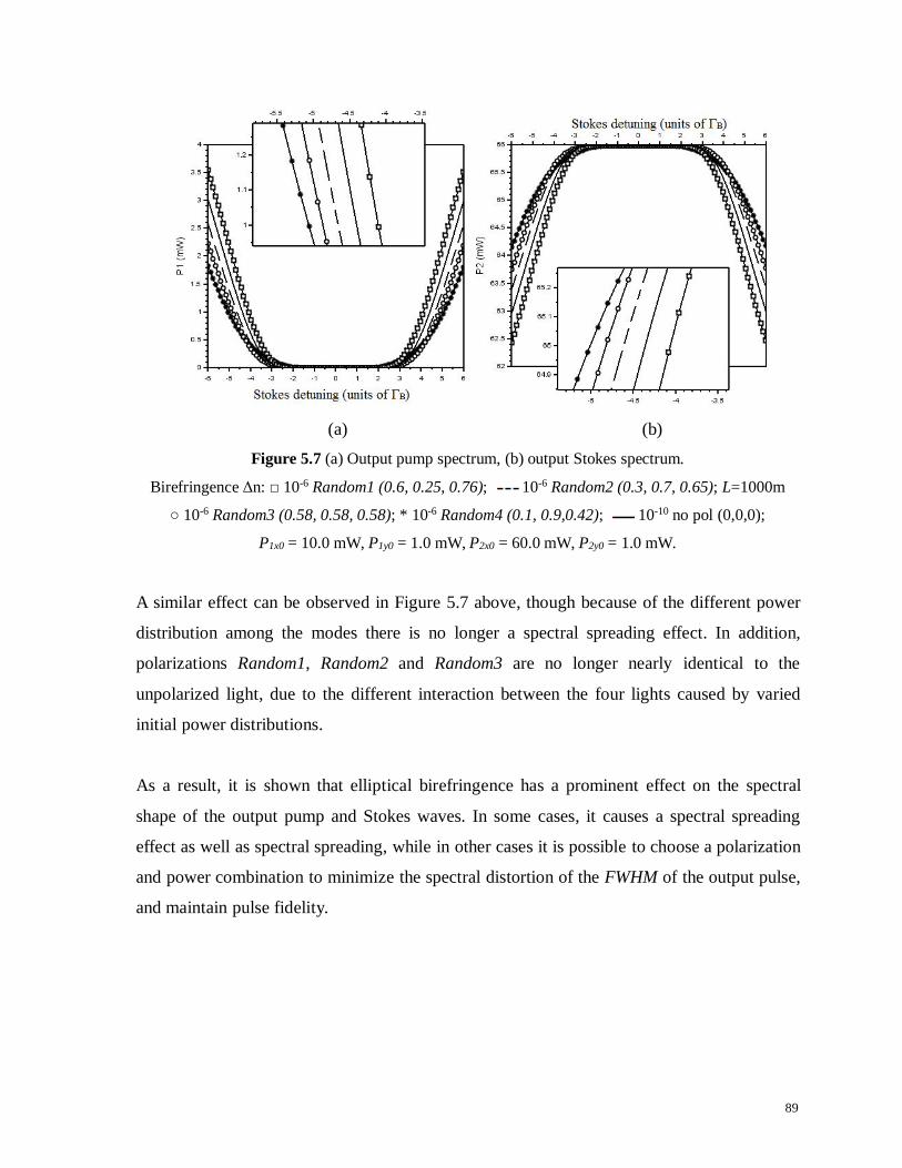
89
(a) (b)Figure 5.7 (a) Output pump spectrum, (b) output Stokes spectrum.
Birefringence Δn: 10-6 Random1 (0.6, 0.25, 0.76); 10-6 Random2 (0.3, 0.7, 0.65); L=1000m
10-6 Random3 (0.58, 0.58, 0.58); * 10-6 Random4 (0.1, 0.9,0.42); 10-10 no pol (0,0,0);
P1x0 = 10.0 mW, P1y0 = 1.0 mW, P2x0 = 60.0 mW, P2y0 = 1.0 mW.
A similar effect can be observed in Figure 5.7 above, though because of the different power
distribution among the modes there is no longer a spectral spreading effect. In addition,
polarizations Random1, Random2 and Random3 are no longer nearly identical to the
unpolarized light, due to the different interaction between the four lights caused by varied
initial power distributions.
As a result, it is shown that elliptical birefringence has a prominent effect on the spectral
shape of the output pump and Stokes waves. In some cases, it causes a spectral spreading
effect as well as spectral spreading, while in other cases it is possible to choose a polarization
and power combination to minimize the spectral distortion of the FWHM of the output pulse,
and maintain pulse fidelity.

90
5.4 Summary
In summary, it has been observed that the degree of birefringence, or beat length, is
responsible for an observed Brillouin shift, ΔυB, in the output PW and SW spectra, which
may be used to quantify the birefringence of the fiber. Polarization and elliptical
birefringence has a prominent effect on the spectral shape of output light – in particular, non-
ideal LP light causes spectral distortion, which appears in the shape of a 'blip' on top of the
expected spectral shape, as well as spreading of the spectrum in the frequency domain. As
such, a good measure for detecting non-ideally linearly polarized light has been established.
Additionally, the spectral depletion of the non-ideally linearly polarized light has uncovered
a regime which is preferable for measurement in sensing applications. Elliptical polarization,
for moderate input powers of the PW and SW, also causes the spectrum to spread out in the
frequency domain. For high input powers, a spectral spreading effect is observed for certain
elliptical polarizations. Other elliptical polarizations provide means for maintaining the
FWHM and pulse fidelity of the Brillouin spectral shape – even for powers beyond the
Brillouin threshold.

91
Chapter 6
Polarization Effects in combined Brillouin gain and loss
6.1 Introduction
In this chapter, a more accurate model of the polarization-dependent Brillouin gain and loss
interaction, which includes the case of elliptical birefringence, is provided. The model
presented in this manuscript describes the most comprehensive equations considering the
birefringence effects in an optical fiber, being an extension of the work presented in Chapter
5. As in Chapter 5, the model includes the most general case of elliptical birefringence, the
effects of polarization mode dispersion (PMD), polarization dependent loss (PDL), phonon
resonance structures, pulse length, as well as the overall attenuation of the fiber.
For sensing applications involving optical differential parametric amplification in Brillouin
optical time domain analysis (ODPA-BOTDA) systems [65, 89], which employ both Stokes
wave (SW) and anti-Stokes wave (ASW) pulses, this investigation of the effects of
birefringence on the combined Brillouin gain and loss is paramount. Additionally, since
spectral distortion is detrimental in sensing applications, it is important to investigate a power
regime in which birefringence effects are minimal.
6.2 Model
The process of Brillouin gain and loss has been studied in a birefringent optical fiber, with a
core radius of 4.1μm. The configuration is comprised of a pump wave (PW) launched into
one end, and a Stokes wave (SW) and an anti-Stokes wave (ASW) launched from the other
end. The PW, SW and ASW have x- and y- eigen-polarization components. The schematic
arrangement is shown in Figure 6.1 below.

92
Figure 6.1 Schematic arrangement of SBS in an optical fiber of length L.
E1x – Pump wave, E1y – Pump wave, E2x – Stokes wave, E2y – Stokes wave, E3x – anti-Stokes wave,
E3y – anti-Stokes wave
The extended system of equations (1.1)-(1.6) describes the interaction of the pump, SW and
ASW, as shown in Figure 6.1, including the effects of PMD and PDL, similar to the system
presented in section 5.2. Again, besides the usual slowly varying amplitude approximation,
the only additional approximation employed was the assumption that the phonon fields are
established almost simultaneously [1, 30].
StokesantiEEE
ivci
EEEivc
i
StokesEEE
ivci
EEEivc
i
Ec
nit
Ecn
zE
yxyyxBASW
Bxy
e
xxxxxBASW
Bxx
e
yxyyxBSW
Bxy
e
xxxxxBSW
Bxx
e
xxx
313*31
2
20
21
2
313*31
2
20
21
2
212*21
1
20
21
2
212*21
1
20
21
2
1111
1111
121
2
12
121
2
12
121
2
12
121
2
12
22
SS
SS
SS
SS
(6.1)

93
StokesantiEEE
ivci
EEEivc
i
StokesEEE
ivci
EEEivc
i
Ec
nit
Ecn
zE
xyxxyBASW
Byx
e
yyyyyBASW
Byy
e
xyxxyBSW
Byx
e
yyyyyBSW
Byy
e
yyy
313*31
2
20
21
2
313*31
2
20
21
2
212*21
1
20
21
2
212*21
1
20
21
2
1111
1111
121
2
12
121
2
12
121
2
12
121
2
12
22
SS
SS
SS
SS
(6.2)
211
*12
1
20
22
2
211*12
1
20
22
2
2222
2222
121
2
12
121
2
12
22
xyyyxBSW
Byx
e
xxxxxBSW
Bxx
e
xxx
EEEivc
i
EEEivc
i
Ec
nit
Ecn
zE
SS
SS
(6.3)
211
*12
1
20
22
2
211*12
1
20
22
2
2222
2222
121
2
12
121
2
12
22
yxxxyBSW
Bxy
e
yyyyyBSW
Byy
e
yyy
EEEivc
i
EEEivc
i
Ec
nit
Ecn
zE
SS
SS
(6.4)

94
311
*13
2
20
22
2
311*13
2
20
23
2
3333
3333
121
2
12
121
2
12
22
xyyyxBASW
Byx
e
xxxxxBASW
Bxx
e
xxx
EEEivc
i
EEEivc
i
Ec
nit
Ecn
zE
SS
SS
(6.5)
311
*13
2
20
22
2
311*13
2
20
23
2
3333
3333
121
2
12
121
2
12
22
yxxxyBASW
Bxy
e
yyyyyBASW
Byy
e
yyy
EEEivc
i
EEEivc
i
Ec
nit
Ecn
zE
SS
SS
(6.6)
For the Stokes wave, we have 2211 xxSWBxx nn
cv
, 2211 yySWByy nn
cv
,
2211 yxSWBxy nn
cv
, 2211 xySWByx nn
cv
, and for the anti-Stokes wave we have
3311 xxASWBxx nn
cv
, 3311 yyASWByy nn
cv
, 3311 yxASWBxy nn
cv
,
3311 xyASWByx nn
cv
, which are the Brillouin frequencies associated with the principal
axis beatings [4], where ω1 is the angular frequency of the PW, and ω2 and ω3 are the angular
frequencies of the SW and ASW respectively. n1x and n1y, n2x and n2y, and n3x and n3y, are the
indices of refraction associated with the principal axes of the PW, SW and ASW respectively.
211 is the angular frequency of the AW1 caused by the interaction of the PW and
SW, and 132 is the angular frequency of the AW2 caused by the interaction of the
PW and ASW. E1x and E1y, E2x and E2y, and E3x and E3y, are the complex amplitudes of the
PW, SW and the ASW, respectively. c is the speed of light, ρ0 is the mean density of the fiber,
γe is the electrostrictive constant, z is the coordinate along the fiber, v is the speed of sound in
the fiber, ΓB is the Brillouin linewidth, and finally, α1x, α1y, α2x, α2y, α3x, and α3y represent the

95
fiber attenuations of the principal axes of polarization of the three interacting waves.
The S1x, S1y, S2x, S2y, S3x, and S3y represent the Stokes vectors in the Poincaré sphere
polarization representation [66, 67], and are used to define the polarization of the
propagating lights [61, 66, 67]. As defined in section 5.2, relations of importance include: Sx1
= -Sy1, Sx2 = -Sy2 and Sx3 = -Sy3. In the above system of equations (6.1)-(6.6), Sx1 describes the
principal state of polarization vector for the forward propagating light, and Sx2 and Sx3
describe the principal states of the polarization vector of the backward propagating lights. In
this case, if Sx1 is defined as Sx1 = (a, b, c), then Sy1 = (-a, -b, -c), Sx2 = (a, b, -c), Sy2 = (-a, -b,
c), Sx3 = (a, b, -c) and Sy3 = (-a, -b, c), where a, b and c are the Stokes vector components
normalized such that a2 + b2 + c2 = 1. For fibers having elliptical birefringence (0 < |c| < 1),
the most general beating situation will be excited.
Lastly, the remaining simplifications were introduced to the system of equations (6.1)-(6.6)
to make the birefringence effect more explicit,2
iyixi
nnn
, iyixi nnn ,
2iyix
i
,
iyixi , i=1,2,3.
In the above arrangement, the PW input parameters are known only at the beginning of the
fiber, i.e. at z=0. Correspondingly, the SW and ASW input parameters are known only at the
end of the fiber, i.e. at z=L, where L is the length of the fiber. Therefore, the boundary
conditions for the system of equations (1.1)-(1.6) are similar to previously-studied
configurations with one pulse [4, 9] from section 5.2. The conditions for two pulses are as
follows
|E1x(0)|2=E21x0; |E1y(0)|2=E21y0 (6.7)
|E2x(L)|2=E22x0; |E2y(L)|2=E22y0 (6.8)
|E3x(L)|2=E23x0; |E3y(L)|2=E23y0 (6.9)
where E21x0 , E21y0 , E22x0 , E22Y0 , E23x0 , and E23y0 are the known squared absolute values of
the complex fields E1x , E1y , E2x , E2y , E3x , and E3y respectively. The same method was used
to simplify the system of equations (6.1)-(6.6) as in section 5.2, namely we have employed

96
the dimensionless length variable Lz / , and the dimensionless time variable ctt / ,
wherecnL
t avgc
is the transit time, navg is the average index of refraction, and r is the
radius of the fiber core. The dimensionless intensity variables are defined as the ratio of
powers Yij=Pij/Pij0, i=1,2,3, j=x,y. Additionally, ε1x, ε1y, ε2x, ε2y, ε3x, and ε3y are the
dimensionless loss terms, defined as ijij L 2 , i=1,2,3, j=x,y. The form factor component
of the β-coefficients is defined as
2
1
B
BijSWij
or
2
2
B
BijASWij
, where i=x,y, j=x,y.
Similarly, the Method of Characteristics [61, 75, 76] was employed as in section 5.2, and the
following change of variables was used n
u 1and
nv 1
, where the
approximation nnn 21 was employed. The resulting system of equations is as follows,
with β-coefficients as defined in expressions (6.16)-(6.31).
xx
Stokesanti
xybxa
Stokes
xybxax YYYYYYY
dudY
1113232121211
(6.10)
yy
Stokesanti
yxdyc
Stokes
yxdycy YYYYYYY
dudY
1113232121211
(6.11)
xxxybxax YYYY
dvdY
22213132 (6.12)
yyyxdycy YYYY
dvdY
22213132 (6.13)
xxxybxax YYYY
dvdY
33314143 (6.14)
yyyxdycy YYYY
dvdY
33314143 (6.15)
221
022
0222
11
1214
SWxx
xx
B
xea cvnr
LPk
SS (6.16) 231
032
0322
211
214
ASWxx
xx
B
xea cvnr
LPk
SS (6.20)

97
221
022
0222
11
1214
SWxy
yx
B
yeb cvnr
LPk
SS(6.17)
221
022
0222
11
1214
SWyy
yy
B
yec cvnr
LPk
SS(6.18)
221
022
0222
11
1214
SWyx
xy
B
xed cvnr
LPk
SS(6.19)
231
032
0322
21
1214
ASWxy
yx
B
yeb cvnr
LPk
SS(6.21)
231
032
0322
21
1214
ASWyy
yy
B
yec cvnr
LPk
SS(6.22)
231
032
0322
21
1214
ASWyx
xy
B
xed cvnr
LPk
SS(6.23)
221
2
1
2
012
0122
31
1214
SWxx
xx
B
xea cvnr
LPk
SS (6.24)
221
2
1
2
012
0122
31
1214
SWyx
xy
B
yeb cvnr
LPk
SS
(6.25)
221
2
1
2
012
0122
31
1214
SWyy
yy
B
yec cvnr
LPk
SS
(6.26)
221
2
1
2
012
0122
31
1214
SWxy
yx
B
xed cvnr
LPk
SS
(6.27)
231
2
1
3
012
0122
411
214
ASWxx
xx
B
xea cvnr
LPk
SS (6.28)
231
2
1
3
012
0122
41
1214
ASWyx
xy
B
yeb cvnr
LPk
SS
(6.29)
231
2
1
3
012
0122
41
1214
ASWyy
yy
B
yec cvnr
LPk
SS
(6.30)
231
2
1
3
012
0122
41
1214
ASWxy
yx
B
xed cvnr
LPk
SS
(6.31)
Once again, the change of variables u and v transforms the system of equations (6.1)-(6.6) of
counter-propagating waves into the system of equations (6.10)-(6.15) of co-propagating
waves. Consequently, we are able to set the initial conditions as
1tanhtanh0, 22110 btabtatYij , each of which takes place at the same end
of the new coordinate system, where i=1,2,3 and j=x,y. The parameters a1 and a2 determine
the rise time of the PW, SW and ASW pulse profiles, while the parameters b1 and b2 define
the center of the pulses via the expression |b2-b1|/2.
In this chapter, the sixth order Runge-Kutta method (RK6) was used to numerically solve the
system of equations (5.1)-(5.6), and was chosen for its stability, increased accuracy and
relatively large step size [90, 91].

98
6.3 Results and Discussion
Output spectra were calculated by detuning the Stokes and anti-Stokes frequencies, ω2 and
ω3, synchronously, as done in the typical experimental setup [4, 28, 92]. Output powers were
calculated as Pij-out=Pij0 ∙Yij-out , i=1,2,3 and j=x,y, and the total power of the pump, Stokes
and anti-Stokes waves was calculated to be Pi=Pix+Piy, i=1,2,3. Also, the attenuation in the
fiber has been approximated as αij=α=0.2 dB/km, i=1,2,3 and j=x,y, and the following
parameters of the fiber were used: navg=1.45, γe=0.902, λ=1550nm, ρ0=2.21g/cm3, v=5616m/s,
ΓB=0.1GHz.
For sensing applications such as the ODPA-BOTDA systems [65, 89], the pump and pulse
powers are chosen to be relatively low, with Ppump > Ppulse. In addition, the ODPA system
functions ideally when the SW and ASW are balanced, causing the gain and loss to eliminate
each other, creating a ‘similar’ effect to the substraction process in the differential
pulse-width pair Brillouin optical time-domain analysis (DPP-BOTDA) in the electric
domain. Consequently, for the simulations performed in this chapter, the pump wave was
given a power of P1x=P1y=1mW, while the Stokes and anti-Stokes waves were given
increasing powers from P2x=P2y=P3x=P3y=0.1mW to 0.9mW in nine different simulations.
Elliptical birefringences of Δn = 10-4, 10-5 and 10-6 were investigated, and compared to the
case of negligible birefringence, Δn = 10-10 with Stokes vector S=(0, 0, 0), which has been
taken to be a first-order approximation to truly unpolarized light. A random elliptical
polarization has been assigned to the pulses, having a Stokes vector S=(0.1, 0.9, 0.424),
which corresponds to polarization Random4 from Chapter 5. A pulse length of 7.5ns has been
chosen for the SW and ASW, respectively.
6.3.1. Gain dominant regime
In this section, pulse powers have been chosen to be between 0.1 mW and 0.6mW. As can be
seen from Figure 6.2 below, the output pump spectra look substantially Lorentzian, since the
powers chosen allowed the combined Brillouin gain and loss to operate in the gain dominant

99
regime. By increasing in pulse powers from 0.1mW to 0.6 mW, the Brillouin spectrum
becomes increasingly distorted. This is caused by an imbalance between the gain and loss
processes since the regime is gain dominant, the loss experienced by the pump wave
contributes in creating an asymmetry in the output pump spectra.
(a) (b) (c)
(d) (e) (f)Figure 6.2 Output pump spectra. S=(0.1, 0.9, 0.42). L=45m. P1x=P1y=1mW.
(a) P2x=P2y=P3x=P3y=0.1mW; (b) P2x=P2y=P3x=P3y=0.2mW; (c) P2x=P2y=P3x=P3y=0.3mW;
(d) P2x=P2y=P3x=P3y=0.4mW; (e) P2x=P2y=P3x=P3y=0.5mW; (f) P2x=P2y=P3x=P3y=0.6mW.
:Δn =10-4; :Δn =10-5; : Δn =10-6; : Δn =10-10 S=(0, 0, 0).
Similar physical principles govern the SBS interaction as described in section 5.3, namely
that in addition to the contributing gain and loss processes, birefringence of the optical fiber
causes the appearance of a fast and slow axis, which results in two optical modes in the fiber

100
with different SBS frequency shifts. This causes a mismatch in the corresponding momentum
vectors of the acoustic waves, thereby making it impossible for both principal axes to be
resonant with the acoustic phonons. The mismatch in phonon resonance causes a Brillouin
shift, ΔυB.
For each power distribution, the spectral shift was calculated for each degree of birefringence,
shown in Figure 6.3(A) below.
(A) (B)Figure 6.3. (A) ΔυB dependence on Δn; (B) Ratio dependence on Δn. L=45m, S=(0.1, 0.9, 0.42).
(a) P2x=P2y=P3x=P3y=0.1mW; (b) P2x=P2y=P3x=P3y=0.2mW; (c) P2x=P2y=P3x=P3y=0.3mW;
(d) P2x=P2y=P3x=P3y=0.4mW; (e) P2x=P2y=P3x=P3y=0.5mW; (f) P2x=P2y=P3x=P3y=0.6mW.
It is apparent from Figure 6.3(A) that the degree of birefringence has a nonlinear effect on
the Brillouin shift ΔυB, in particular, the larger the birefringence, the larger the shift,
regardless of the power distribution. Not surprisingly, this nonlinear effect is similar to the
case of the two-wave interaction of the PW and SW from Chapter 5. This spectral shift can in
turn be used to quantify the birefringence of the optical fiber upon measurement of the output
signal. Understandably, the largest shifts occur for the smallest power disparity between the
pump and pulses, while the smallest shift occurs for the largest power disparity, since the
case of smaller power disparity, shown in Figure 6.2(f), yields a greater spectral distortion
due to a stronger competing gain and loss process, while the spectral distortion of Figure
6.2(a) is nearly noticeable.
To assess the effect of birefringence on the asymmetry of the output spectra, the spectral
width at half maximum on the left, ΔυL, and the spectral width at half maximum on the right,

101
ΔυR, was measured, and their Ratio=ΔυL/ΔυR was calculated. Exemplary ΔυL and ΔυR are
shown in Figure 6.2(f) for clarity a perfectly symmetric spectrum would have a Ratio=1.
Figure 6.3(B) below shows the Ratios for the different power distributions, as well as for
different Δn, from which it is confirmed that an increase in pulse power increases the spectral
distortion (asymmetry) of the output plots. Although the general asymmetrical shape is a
result of the competing gain and loss processes, an increase in birefringence contributes to
the asymmetry, increasing the disparity between ΔυL and ΔυR, as seen by the increase in the
Ratio, as compared to the case of negligible birefringence.
In the most general case of elliptical birefringence used in both Chapter 5 and the current
chapter, there are four running acoustic waves, each having their own resonance frequency.
As a result, each of the fast and slow modes have their own resonant frequency at which
energy transfer occurs. The result is an asymmetric spectral shape due to the uneven energy
transfer along different resonant frequencies. The effects of polarization mode dispersion
(PMD) contribute to the spectral distortion seen in Figure 6.3(B), since the existence of a fast
and slow axis causes the two optical modes to travel at different speeds, and arrive at the end
of the fiber at differing times. In Chapter 5, this has been shown to causes a spectral
spreading, and in combination with the multiple resonance frequencies, could account for the
increase in distortion.

102
6.3.2 Competing Gain and Loss regime
In the previous section, although the gain and loss processes were competing, due to the
power distributions chosen, the regime was mainly gain dominant. For higher pulse powers,
the loss process becomes stronger, making the effects of the gain and loss regime comparable.
In this section, pulse powers were increased from 0.7mW to 0.9mW.
(a) (b) (c)
Figure 6.4 Output pump spectra. S=(0.1, 0.9, 0.42). L=45m. P1x=P1y=1mW.
(a) P2x=P2y=P3x=P3y=0.7mW; (b) P2x=P2y=P3x=P3y=0.8mW; (c) P2x=P2y=P3x=P3y=0.9mW;
:Δn =10-4; :Δn =10-5; : Δn =10-6; : Δn =10-10 S=(0, 0, 0).
As can be seen from Figure 6.4, the comparable gain and loss processes substantially alter
the output pump spectrum from its previous Lorentzian shape [28, 30] in Figure 6.4(a) the
spectral deformity results in dual peaks, or a spectral spreading effect, while in Figures
6.4(b)-(c) there is a simultaneous gain and loss spectra. A spectral shift is still apparent in
Figure 6.4(a), the positions of the two peaks have been measured, while in Figures 6.4(b)-(c)
the positions of the peaks and troughs have been measured. The results are shown in Figure
6.5(A) below, where the same general trend is observed as in Figure 6.3(A).
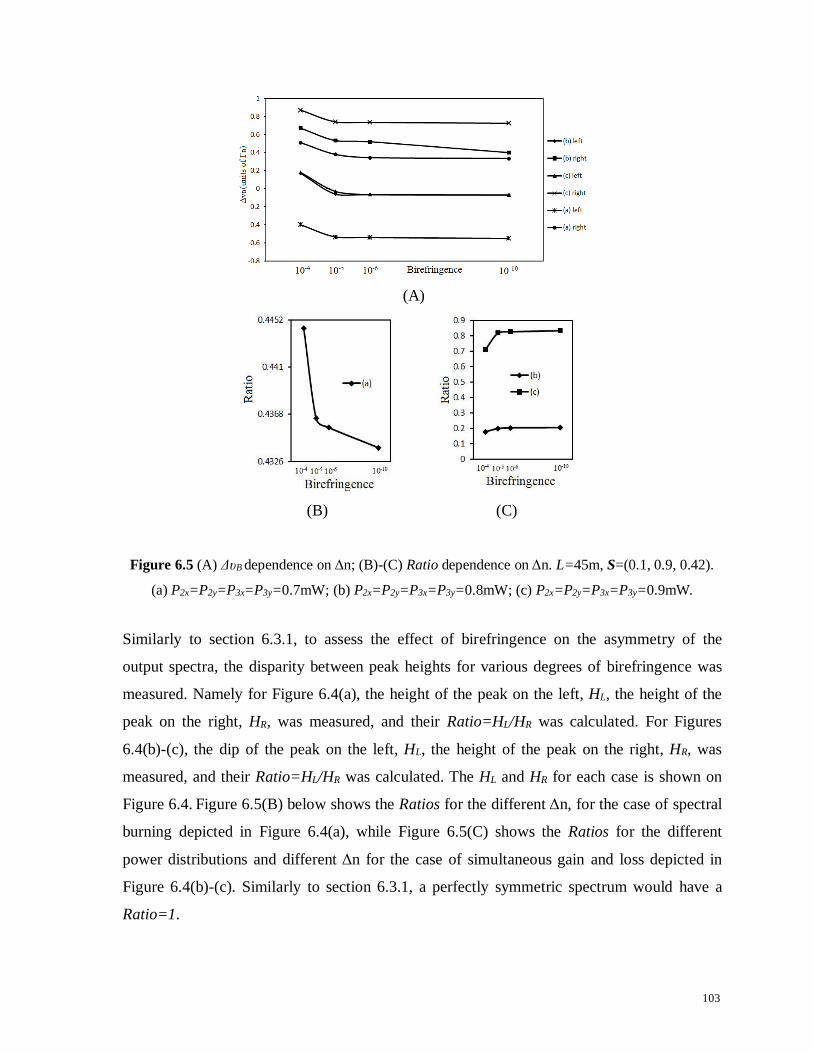
103
(A)
(B) (C)
Figure 6.5 (A) ΔυB dependence on Δn; (B)-(C) Ratio dependence on Δn. L=45m, S=(0.1, 0.9, 0.42).
(a) P2x=P2y=P3x=P3y=0.7mW; (b) P2x=P2y=P3x=P3y=0.8mW; (c) P2x=P2y=P3x=P3y=0.9mW.
Similarly to section 6.3.1, to assess the effect of birefringence on the asymmetry of the
output spectra, the disparity between peak heights for various degrees of birefringence was
measured. Namely for Figure 6.4(a), the height of the peak on the left, HL, the height of the
peak on the right, HR, was measured, and their Ratio=HL/HR was calculated. For Figures
6.4(b)-(c), the dip of the peak on the left, HL, the height of the peak on the right, HR, was
measured, and their Ratio=HL/HR was calculated. The HL and HR for each case is shown on
Figure 6.4. Figure 6.5(B) below shows the Ratios for the different Δn, for the case of spectral
burning depicted in Figure 6.4(a), while Figure 6.5(C) shows the Ratios for the different
power distributions and different Δn for the case of simultaneous gain and loss depicted in
Figure 6.4(b)-(c). Similarly to section 6.3.1, a perfectly symmetric spectrum would have a
Ratio=1.
104
The spectral spreading effect of Figure 6.4(a) can be explained as a result of a sufficiently
strong loss process, which causes a portion of the pump spectra to become substantially
depleted, but not sufficiently strong enough to create a lossy spectrum. From Figure 6.5(A),
it can be seen that the disparity between the height of the peaks increases with increasing
birefringence, represented by the decreasing Ratio birefringence contributes once again to
spectral asymmetry.
However, looking at Figure 6.5(C), it is apparent that with increasing birefringence, the
disparity between the gain and loss peaks decreases, represented by the Ratio becoming
closer to 1, hence the asymmetry decreases. This can be explained by the same multiple
resonant frequency argument as in section 6.3.1. The same energy transfer that contributed to
the increase in spectral asymmetry in section 6.3.1, now contributes to creating a more
symmetrical simultaneous gain and loss spectrum in Figures 6.4(b)-(c).
As can be seen from Figures 6.2 and 6.4 above, the effects of PMD and PDL caused by
birefringence result in a spectral distortion effect, similar to the one reported in [28] for
BOTDA systems. Since elliptical polarizations of the interacting pulses include vertical,
horizontal, and circular components in their Stokes vectors, it is therefore expected that the
resulting gain would be different than in the case of parallel linear alignment, where both
waves have the Stokes vector (1, 0, 0) and experience maximum gain along one resonant
frequency [22, 24, 25]. In the case of elliptical polarization, where there exists an interaction
along all components of the Poincaré sphere, an increase in distortion effects is expected, as
compared to the case of perfectly parallel polarized light, often attributed to models of
Brillouin gain and loss which do not account for polarization [4, 65, 89]. In the gain
dominant regime, this distortion contributes to the asymmetry of the output pump spectrum,
while conversely in the competing gain and loss regime, the distortion contributes to making
the output spectra more symmetrical.
The spectral distortion effect is highly detrimental for the ODPA-BOTDA sensor system
employing Lorentzian spectra [65, 89], where an inaccurate spectral reading could cause
inaccuracies in the operation of the sensor. Based on the results of this chapter, it is therefore

105
beneficial to choose powers in the gain dominant regime. Not only is the output pump
spectrum substantially Lorentzian in this regime, but the higher the disparity in power
between the pump and pulses, the more minimal the effect of birefringence is on the spectral
distortion of the output pulse.
6.4 Summary
The most general model of elliptical birefringence in an optical fiber has been extended to
describe a transient Brillouin interaction including both gain and loss. Spectral distortion
effects related to birefringence have been investigated in the gain dominant and competing
gain and loss regimes. It has been shown that the spectral distortion caused by birefringence
can be minimized by choosing pump and pulse powers with a large disparity.

106
Chapter 7
Applications of SBS: Photonic Logic
7.1 Introduction
In this chapter, a novel fiber nonlinearity-based technique is proposed to realize all-optical
NAND/NOT/AND/OR logic gates, based on the principles of a combined Brillouin gain and
loss process in a polarization maintaining fiber (PMF). Combined Brillouin gain and loss is
often advantageous over Brillouin gain in the construction of all-optical gates since it
describes the energy transfer between three optical waves, as compared to only two optical
waves. Additionally, the combination of simultaneous gain and loss acts to improve the
signal-to-noise ratio (SNR) by approximately twofold [92] upon measurement of the
Brillouin gain spectrum (BGS). This increases the clarity of the signal, as well as the
switching contrast in the proposed logic gates. Furthermore, the combined gain and loss
scheme is more compact than the traditional Brillouin optical correlation-domain analysis
(BOCDA) system [93, 94], which employs successive utilization of the Brillouin gain and
loss. The additional parameters in the three-wave interaction give combinations of input
powers such that the output signals yield results which correspond to the truth tables of, for
example, a NAND gate. The combined Brillouin gain and loss model was used to create
several configurations of a functional NAND gate, and a NOT gate. With Brillouin gain one
can construct a simplified NOT gate. The combination of the NAND and NOT gates has
been used to further construct several configurations of AND and OR gates. Switching
contrasts are simulated to be between 20-83% for various configurations.
7.2 Model
The process of combined Brillouin gain and loss has been studied in a single mode optical
fiber, with core radius of 4.1μm and power penalty of 0.67 dB/km. The configuration is

107
comprised of a pump wave, which has been taken to be a continuous wave (CW) launched
into one end, and a Stokes wave (SW), and an anti-Stokes wave (ASW) launched into the
other end. The schematic arrangement is shown on Figure 2.8 in Chapter 2. Since the pump
wave is a continuous wave in this case, it will be referred to as ‘CW.’
The system is deemed to operate in the steady-state regime with pulse lengths greater than
the phonon relaxation time, in this case 10ns [1, 4]. In the slowly varying amplitude
approximation, the steady state interaction between the CW, SW, ASW and two acoustic
waves (AW1 and AW2) is described by the system of equations (2.33)-(2.37) from Chapter 2,
shown again below [1, 9, 65].
13*2
0
121
0
11
21
22AA
nciA
nci
dzdA ee
(7.1)
21*1
0
22
21
2AA
nci
dzdA e
(7.2)
3120
33
21
2AA
nci
dzdA e
(7.3)
*21
21
1121
2
4AAqi e
BB (7.4)
*13
22
2222
2
4AAqi e
BB (7.5)
Where Ω1=ω1 – ω2, Ω2=ω3 – ω1, Ω1 is the angular frequency of the AW1 caused by the
interaction of CW and SW, Ω2 is the angular frequency of the AW2 caused by interaction of
CW and ASW, q1 and q2 are the acoustic wavevectors defined as q1≈2k1 and q2≈2k1, where
k1 is the wavevector of the CW, defined as |k1|=nω1/c. A1 is the complex amplitude of the
CW, A2 is the complex amplitude of the SW, A3 is the complex amplitude of the ASW, ρ1 is
the complex amplitude of the AW1 caused by interaction of CW and SW, ρ2 is the complex
amplitude of the AW2 caused by interaction of CW and ASW, c is the speed of light, ρ0 is the
density of the fiber, γe is the electrostrictive constant, z is the coordinate along the fiber, n is
the index of refraction of the fiber, v is the speed of sound in the fiber, ΓB is the Brillouin
linewidth, ΩB is the Brillouin frequency defined as ΩB = 2nvω1/c, where ω1 is the angular

108
frequency of the CW, ω2 is the angular frequency of the SW, and ω3 is the angular frequency
of the ASW.
For a two-wave configuration describing Brillouin gain, the ASW terms are simply set to ‘0’
in the following analysis. In the above arrangement, the SW and ASW input parameters are
known only at the beginning of the fiber, i.e. at z=0. Correspondingly, the CW input
parameters are known only at the end of the fiber, i.e. at z=L, where L is the length of the
fiber. Therefore, the boundary conditions for the system of equations (7.1)-(7.5) are similar
to previously-studied configurations with one pulse [4, 65]. The conditions for two pulses are
as follows
|A1(L)|2 = A210; |A2(0)|2 =A220; |A3(0)|2 =A230 (7.6)
where A210 , A220 and A230 are known squared absolute values of the complex amplitudes A1 ,
A2 , and A3 respectively. In the dimensionless notation, the system of equations (7.1)-(7.5)
becomes
13122111 YYYYY
dldY (7.7)
22132 YYY
dldY (7.8)
33143 YYY
dldY (7.9)
2154 YYY (7.10)
3165 YYY (7.11)
With corresponding boundary conditions: Y1(1)=1; Y2(0)=1; Y3(0)=1 (7.12)
The dimensionless variables Lzl / , Y1=P1/P10, Y2=P2/P20, Y3=P3/P30, Y4=|ρ1/ρ0|2,
Y5=|ρ2/ρ0|2, L have been introduced to derive the system of equations (7.7)-(7.11), as
well as the following β-coefficients.
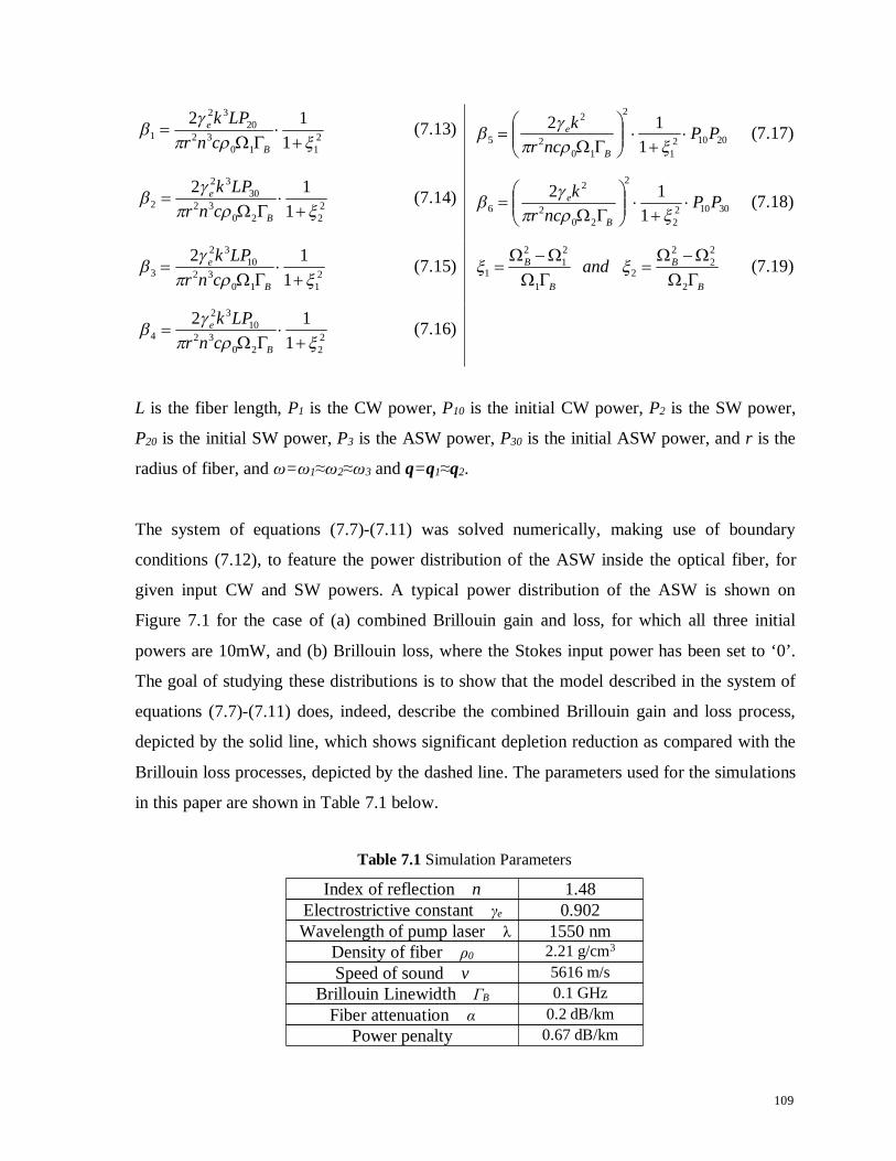
109
2110
3220
32
1 112
B
e
cnrLPk (7.13)
201021
2
102
2
5 112 PP
ncrk
B
e
(7.17)
2220
3230
32
2 112
B
e
cnrLPk (7.14)
301022
2
202
2
6 112 PP
ncrk
B
e
(7.18)
2110
3210
32
3 112
B
e
cnrLPk (7.15)
B
B
B
B and
2
22
2
21
21
2
1 (7.19)
2220
3210
32
4 112
B
e
cnrLPk (7.16)
L is the fiber length, P1 is the CW power, P10 is the initial CW power, P2 is the SW power,
P20 is the initial SW power, P3 is the ASW power, P30 is the initial ASW power, and r is the
radius of fiber, and ω=ω1≈ω2≈ω3 and q=q1≈q2.
The system of equations (7.7)-(7.11) was solved numerically, making use of boundary
conditions (7.12), to feature the power distribution of the ASW inside the optical fiber, for
given input CW and SW powers. A typical power distribution of the ASW is shown on
Figure 7.1 for the case of (a) combined Brillouin gain and loss, for which all three initial
powers are 10mW, and (b) Brillouin loss, where the Stokes input power has been set to ‘0’.
The goal of studying these distributions is to show that the model described in the system of
equations (7.7)-(7.11) does, indeed, describe the combined Brillouin gain and loss process,
depicted by the solid line, which shows significant depletion reduction as compared with the
Brillouin loss processes, depicted by the dashed line. The parameters used for the simulations
in this paper are shown in Table 7.1 below.
Table 7.1 Simulation Parameters
Index of reflection n 1.48Electrostrictive constant γe 0.902Wavelength of pump laser λ 1550 nm
Density of fiber ρ0 2.21 g/cm3
Speed of sound v 5616 m/sBrillouin Linewidth ΓB 0.1 GHz
Fiber attenuation α 0.2 dB/kmPower penalty 0.67 dB/km

110
Figure 7.1 ASW power distribution inside the optical fiber.
(a) Gain and Loss regime: P20=10mW; (b) Loss regime: P20=0mW
n=1.48, γe=0.902, λ=1550nm, ρ0=2.21 g/cm3, v=5616 m/s, ΓB=0.1 GHz, α=0.2 dB/km, L=350m,
P10=10mW, P30=10mW.
7.3 Results and Discussion
It has been determined that obtaining a logical output of exactly 0.1mW or 10mW is not
feasible. However, it is possible to obtain output signals within a given level of tolerance. In
this manuscript, a threshold value of at least 20% is deemed acceptable. Switching contrast
bar graphs are introduced in Figures 7.2, 7.5, 7.6 and 7.9, showing the output signals as
percentages of the optimal signal power of 10mW. The tolerance between the low and high
thresholds is the resultant switching contrast of the logic gate configuration. The higher the
switching contrast, the more accurate the logical ‘0’ and ‘1’ representation is by the real
circuit.
7.4 NAND gate
7.4.1 Configuration I
In Configuration I, a fiber length of L=2300m was used (shorter fiber length is possible with
lower switching contrast), and the ASW reference signal was kept constant at P30=40mW.
The logical output ‘1’ corresponds to several different values of output power, namely
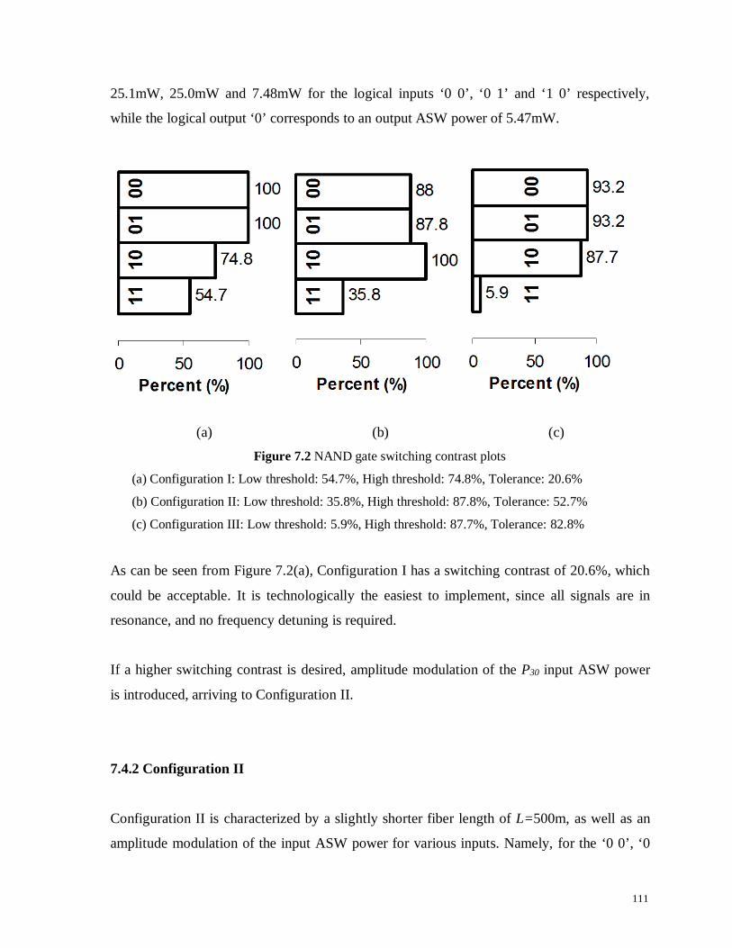
111
25.1mW, 25.0mW and 7.48mW for the logical inputs ‘0 0’, ‘0 1’ and ‘1 0’ respectively,
while the logical output ‘0’ corresponds to an output ASW power of 5.47mW.
(a) (b) (c)Figure 7.2 NAND gate switching contrast plots
(a) Configuration I: Low threshold: 54.7%, High threshold: 74.8%, Tolerance: 20.6%
(b) Configuration II: Low threshold: 35.8%, High threshold: 87.8%, Tolerance: 52.7%
(c) Configuration III: Low threshold: 5.9%, High threshold: 87.7%, Tolerance: 82.8%
As can be seen from Figure 7.2(a), Configuration I has a switching contrast of 20.6%, which
could be acceptable. It is technologically the easiest to implement, since all signals are in
resonance, and no frequency detuning is required.
If a higher switching contrast is desired, amplitude modulation of the P30 input ASW power
is introduced, arriving to Configuration II.
7.4.2 Configuration II
Configuration II is characterized by a slightly shorter fiber length of L=500m, as well as an
amplitude modulation of the input ASW power for various inputs. Namely, for the ‘0 0’, ‘0
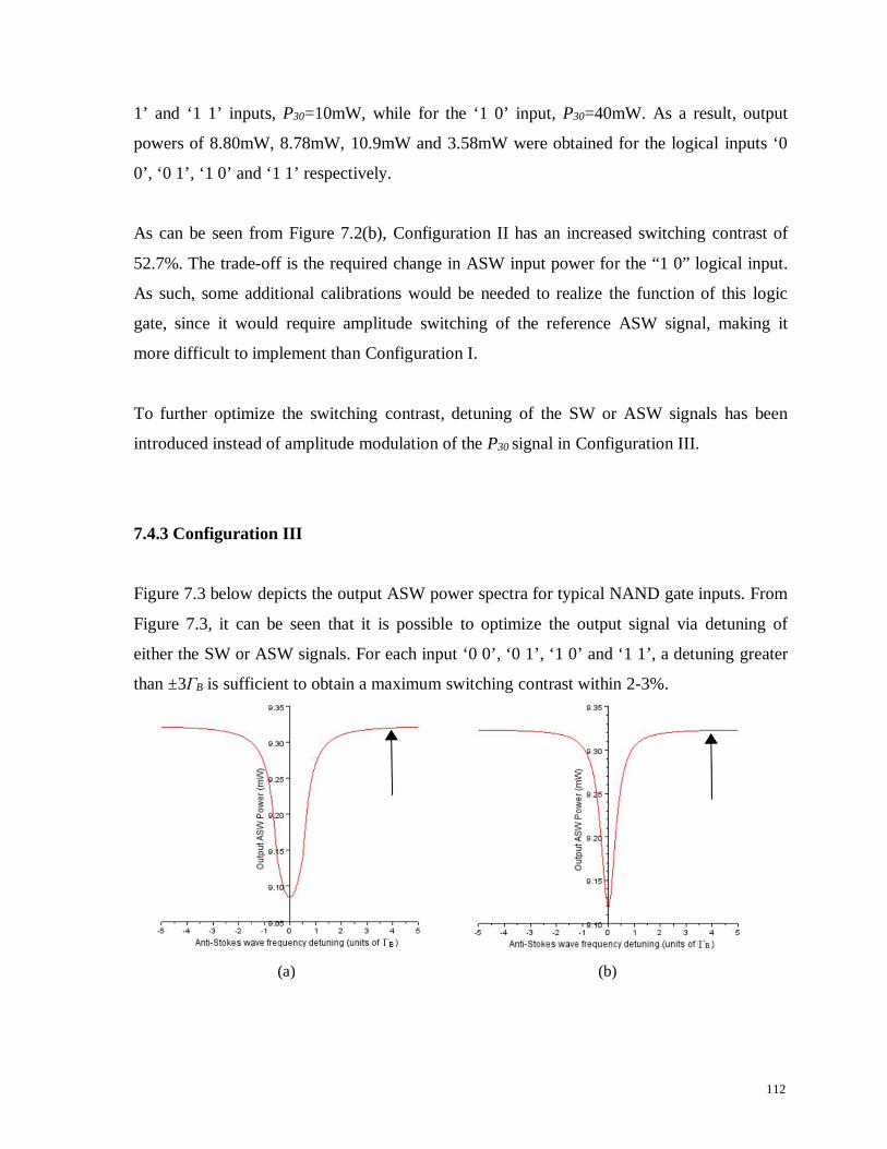
112
1’ and ‘1 1’ inputs, P30=10mW, while for the ‘1 0’ input, P30=40mW. As a result, output
powers of 8.80mW, 8.78mW, 10.9mW and 3.58mW were obtained for the logical inputs ‘0
0’, ‘0 1’, ‘1 0’ and ‘1 1’ respectively.
As can be seen from Figure 7.2(b), Configuration II has an increased switching contrast of
52.7%. The trade-off is the required change in ASW input power for the “1 0” logical input.
As such, some additional calibrations would be needed to realize the function of this logic
gate, since it would require amplitude switching of the reference ASW signal, making it
more difficult to implement than Configuration I.
To further optimize the switching contrast, detuning of the SW or ASW signals has been
introduced instead of amplitude modulation of the P30 signal in Configuration III.
7.4.3 Configuration III
Figure 7.3 below depicts the output ASW power spectra for typical NAND gate inputs. From
Figure 7.3, it can be seen that it is possible to optimize the output signal via detuning of
either the SW or ASW signals. For each input ‘0 0’, ‘0 1’, ‘1 0’ and ‘1 1’, a detuning greater
than ±3ΓB is sufficient to obtain a maximum switching contrast within 2-3%.
(a) (b)

113
(c) (d)
Figure 7.3 Output ASW power spectra.
(a) ‘0 0’ input, (b) ‘0 1’ input, (c) ‘1 0’ input, (d) ‘1 1’ input.
Configuration II utilizes a fiber length of L=350m, as well as detuning of the SW and ASW
to achieve a maximum switching contrast. Namely, for the ‘0 0’, ‘0 1’ and ‘1 0’ inputs, the
ASW is detuned by ±3ΓB, while for the ‘1 1’ input, the SW is detuned by ±3ΓB. As a result,
output powers of 9.32mW, 9.32mW, 8.77mW, and 0.59mW were obtained for the logical
inputs ‘0 0’, ‘0 1’, ‘1 0’ and ‘1 1’ respectively. In this configuration, the reference ASW
signal was held constant at P30=10mW.
Configuration III requires a tunable laser source, capable of detuning the SW and ASW
separately. Although technologically this is more complicated to realize, the tunable
frequency range is very large and, in this case, any detuning outside ±3ΓB (about ±0.3 GHz)
will provide the maximum switching contrast of 82.8%, within 2-3%. As such, this
configuration also benefits from a shorter fiber length of 350m, which acts to compactify the
setup.

114
7.5 NOT gate
7.5.1 Configuration IV
Although, according to DeMorgan’s Theorem [95], any logic gate may be constructed from
several NAND gates, practical considerations may require a simplified design of certain
simple gates, such as the NOT, AND, etc. In view of this, the design for an all-optical NOT
gate was considered, using a similar approach as for the NAND gate described in previous
sections. The combination of the NAND and NOT gates may be used to create a simplified
AND gate, which would require minimal calibration and yield a high switching contrast.
In Configuration IV, the initial CW power, P10 , was chosen to be the input signal, and the
output ASW power, P3-out, was taken to be the output signal of the optical gate. In this case,
the input SW is a reference signal, and was held constant at P20=10mW. As before, a power
of 0.1mW was assigned a logical value of ‘0’, while a power of 10mW was assigned a
logical value of ‘1’. Output powers of 9.11mW and 3.89mW were obtained for the logical
inputs ‘0’ and ‘1’ respectively. In this configuration, a fiber length of L=350m was used.
(a) (b)
Figure 7.4 NOT gate switching contrast plots
(a)Configuration IV: Low threshold: 38.9%, High threshold: 91.1%, Tolerance: 52.9%
(b)Configuration V: Low threshold: 13.3%, High threshold: 90.0%, Tolerance: 77.6%

115
The proposed configuration of the NOT gate has all the technological benefits of the NAND
gate in Configuration I, as well as a switching contrast of 52.9%, as can be seen from Figure
7.4(a).
7.5.2 Configuration V
Another possible realization of the NOT gate utilizes the two-wave configuration of Brillouin
gain. In this case, the initial SW power, P20, was chosen to be the input signal, and the output
CW power, P1-out , was taken to be the output signal of the optical gate. The input CW was
taken to be the reference signal, and was held constant at P10=10mW. A power of 0.1mW
was assigned a logical value of ‘0’, while a power of 10mW was assigned a logical value of
‘1’. Output powers of 9.0mW and 1.33mW were obtained for the logical inputs ‘0’ and ‘1’
respectively. In this configuration, a fiber length of L=350m was used.
As seen in Figure 7.4(b), the proposed configuration of the NOT gate has a higher switching
contrast of 77.6%, as compared to Configuration IV. Additionally, the current NOT gate,
based on the two-wave SBS interaction is substantially simpler in design, requiring the use of
only two optical waves, as compared to three optical waves.
7.6 AND gate
7.6.1 Configuration VI
In the current configuration, an AND gate is constructed by connecting the NAND gate of
Configuration III with the NOT gate of Configuration IV, shown schematically in Figure 7.5
below.

116
Figure 7.5 Schematic of Configuration VI: AND gate.
P10 and P20, represented by CW1 and SW1 in Figure 7.5 above, are the input signals of the
AND gate, while the initial power of the reference signal ASW1 is held constant at
P30=10mW. The output ASW’1 signal from the NAND gate, P3-out, is frequency downshifted
from ω3 to ω1, turning it into an effective CW2 wave, which is the input signal for the NOT
gate. SW2 and ASW2 are the reference signals of the NOT gate, and are kept constant at
10mW. The output signal of the AND gate is the ASW’2 signal. As before, a power of
0.1mW was assigned a logical value of ‘0’, while a power of 10mW was assigned a logical
value of ‘1’. Output powers of 4.02mW, 4.02mW, 4.14mW and 8.31mW were obtained for
the logical inputs ‘0 0’, ‘0 1’, ‘1 0’ and ‘1 1’ respectively. In this configuration, a fiber length
of L=350m was used for both the NAND gate and NOT gate.
(a) (b)
Figure 7.6 AND gate switching contrast plots.
(a) Configuration VI: Low threshold: 40.2%, High threshold: 83.1%, Tolerance: 42.3%
(b) Configuration VII: Low threshold: 16.1%, High threshold: 77.1%, Tolerance: 61.8%

117
The same detuning must be applied to optical signals entering the NAND gate as stated in the
description of Configuration III. For the subsequent NOT gate, input signals should be kept
at resonance.
As can be seen from Figure 7.6(a), Configuration VI of the AND gate yields a switching
contrast of 42.3%.
7.6.2 Configuration VII
In the current configuration, an AND gate is constructed by connecting the NAND gate of
Configuration III with the NOT gate of Configuration V, shown schematically in Figure 7.7
below.
Figure 7.7 Schematic of Configuration VII: AND gate.
Similar to Configuration VI, P10 and P20, represented by CW1 and SW1 in Figure 7.7 above,
are the input signals of the AND gate, while the initial power of the reference signal ASW1 is
held constant at P30=10mW. The output ASW’1 signal from the NAND gate, P3-out, is
frequency downshifted from ω3 to ω2, turning it into an effective SW2 wave, which is the
input signal for the NOT gate. The reference signal CW2 is kept constant at 10mW. The
output signal of the AND gate is the CW’2 signal. As usual, a power of 0.1mW was assigned
a logical value of ‘0’, while a power of 10mW was assigned a logical value of ‘1’. Output
powers of 1.47mW, 1.47mW, 1.61mW and 7.71mW were obtained for the logical inputs ‘0

118
0’, ‘0 1’, ‘1 0’ and ‘1 1’ respectively. Once again, a fiber length of L=350m was used for
both the NAND gate and NOT gate.
The same detuning must be applied to optical signals entering the NAND gate as stated in the
description of Configuration III. For the subsequent NOT gate, input signals should be kept
at resonance.
As can be seen from Figure 7.6(b), Configuration VI of the AND gate yields a switching
contrast of 61.8%. This is higher than the switching contrast on Configuration VI;
additionally, the setup is substantially simpler since the NOT gate from Configuration V
requires a two-wave SBS interaction.
7.6.3 Configuration VIII
In another possible configuration, loops mirrors [96] and High-Order Mode Fibers (HOM)
[97, 98], are utilized to re-use the fiber under test. Loops mirrors redirect output light back
into a different mode of the HOM, thereby compactifying the setup. In this configuration
only one fiber, which must be an HOM fiber, is required. Since HOM fibers do not maintain
the polarization of propagating light, this configuration is more prone to polarization
instabilities and PMD. Another possibility is to use a PMF, whereby loop mirrors redirect
output light back into a perpendicularly polarized state in the same fiber, similar to the
implemented schemes in [99, 100]. This would also act to compactify the setup, while
helping to eliminate the influence of polarization instability and PMD.
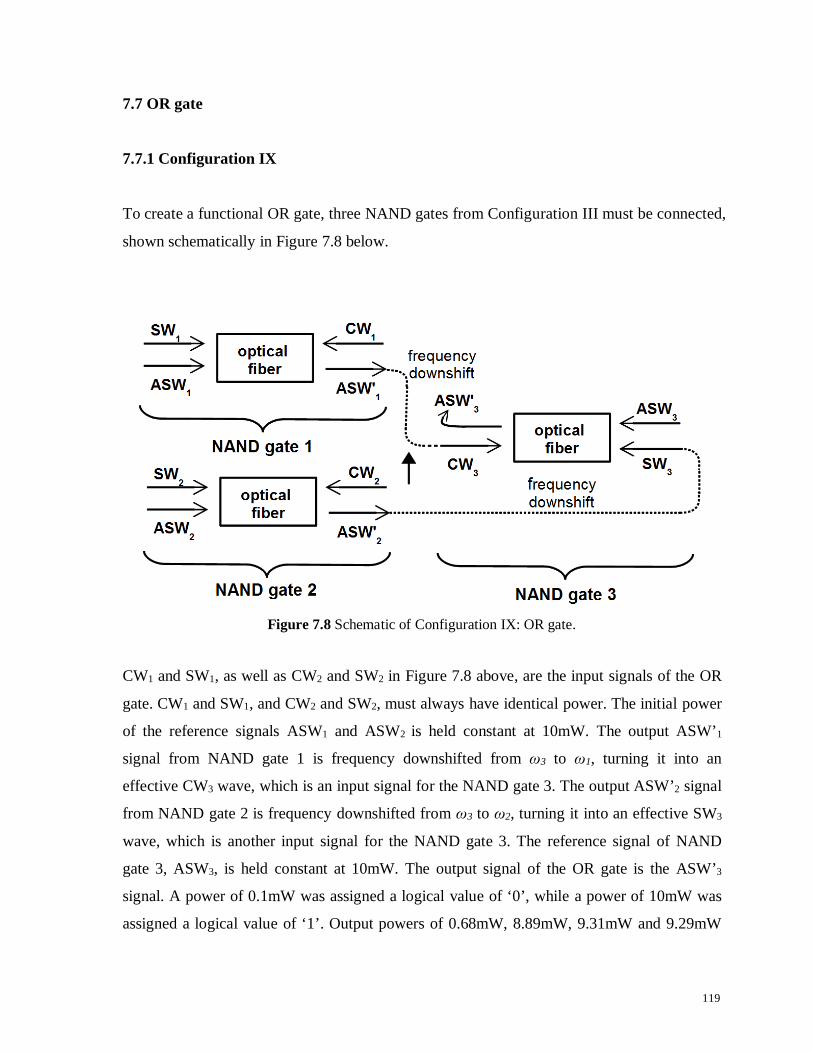
119
7.7 OR gate
7.7.1 Configuration IX
To create a functional OR gate, three NAND gates from Configuration III must be connected,
shown schematically in Figure 7.8 below.
Figure 7.8 Schematic of Configuration IX: OR gate.
CW1 and SW1, as well as CW2 and SW2 in Figure 7.8 above, are the input signals of the OR
gate. CW1 and SW1, and CW2 and SW2, must always have identical power. The initial power
of the reference signals ASW1 and ASW2 is held constant at 10mW. The output ASW’1
signal from NAND gate 1 is frequency downshifted from ω3 to ω1, turning it into an
effective CW3 wave, which is an input signal for the NAND gate 3. The output ASW’2 signal
from NAND gate 2 is frequency downshifted from ω3 to ω2, turning it into an effective SW3
wave, which is another input signal for the NAND gate 3. The reference signal of NAND
gate 3, ASW3, is held constant at 10mW. The output signal of the OR gate is the ASW’3
signal. A power of 0.1mW was assigned a logical value of ‘0’, while a power of 10mW was
assigned a logical value of ‘1’. Output powers of 0.68mW, 8.89mW, 9.31mW and 9.29mW

120
were obtained for the logical inputs ‘0 0’, ‘0 1’, ‘1 0’, and ‘1 1’ respectively. A fiber length
of L=350m was used for all three NAND gates.
The same detuning must be applied to optical signals entering all three NAND gates as stated
in the description of Configuration III.
Figure 7.9 OR gate switching contrast plot.
Low threshold: 6.8%, High threshold: 88.9%, Tolerance: 83.0%.
As can be seen from Figure 7.9, Configuration IX of the OR gate yields a switching contrast
of 83.0%. Though the current configuration is more complicated than the previous ones, it
also yields an extremely high switching contrast.
7.7.2 Configuration X
In the current configuration, an OR gate is constructed by connecting a NAND gate with two
3-wave NOT gates, shown schematically in Figure 7.10 below.

121
(a)(b)
Figure 7.10 (a) Schematic of Configuration X: OR gate, (b) OR gate switching contrast plot,
Low threshold: 7.04%, High threshold: 90.6%, Tolerance: 83.6%.
CW1, as well as CW2, in Figure 7.10(a) above, are the input signals of NOT gate 1 and NOT
gate 2, respectively, as well as the two input signals of the OR gate. Similarly, SW1 and
ASW1, as well as SW2 and ASW2, are the reference signals of each NOT gate, which are
held constant at 10mW. The output ASW’1 signal from NOT gate 1 is frequency downshifted
from ω3 to ω1, turning it into an effective CW3 wave, which is an input signal for the NAND
gate. The output ASW’2 signal from NOT gate 2 is frequency downshifted, from ω3 to ω2,
turning it into an effective SW3 wave, which is another input signal for the NAND gate. The
reference signal of the NAND gate, ASW3, is held constant at 10mW. The output signal of
the OR gate is the ASW’3 signal. Output powers of 0.704mW, 9.24mW, 9.06mW, and
9.19mW were obtained for the logical inputs ‘0 0’, ‘0 1’, ‘1 0’, and ‘1 1’, respectively. A
fiber length of L=350m was used for all three gates.
As can be seen from Figure 7.10(b), Configuration X of the OR gate yields a high switching
contrast of 83.6%. This is comparable to the OR gate proposed in Configuration IX, which
has a switching contrast of 83.0%. Additionally, NOT gate 1 and NOT gate 2 have only one
input each, namely CW1 and CW2 respectively. The SW1 and ASW1, and SW2 and ASW2,
respectively, are kept as reference signals. In the OR gate of Configuration IX, a NAND gate
1 and a NAND gate 2 are employed – each having two input signals, CW1 and SW1, and
CW2 and SW2, respectively, which must be carefully calibrated to match each other for each
logical input. Such calibration is time-consuming, and often difficult to achieve.

122
Configuration X eliminates this difficulty by employing NOT gate 1 and NOT gate 2, which
by virtue of the operation of a NOT gate, have only one input signal each, and do not require
any such calibration. As a result, Configuration X of the all-optical OR gate has the benefit
of being simpler to operate and more compact as compared to the existing variant of
Configuration IX.
7.7.3 Configuration XI
In the current configuration, an OR gate is constructed by connecting a NAND gate with two
2-wave NOT gates, shown schematically in Figure 7.11 below.
(a) (b)Figure 7.11 (a) Schematic of Configuration XI: OR gate, (b) OR gate switching contrast plot,
Low threshold: 7.22%, High threshold: 89.6%, Tolerance: 82.4%.
SW1, as well as SW2, in Figure 7.11(a) above, are the input signals of NOT gate 1 and NOT
gate 2, respectively, as well as the two input signals of the OR gate. Similarly, CW1 and CW2
are the reference signals of NOT gate 1 and NOT gate 2, respectively, which are held
constant at 10mW. The output CW’1 signal from NOT gate 1 is redirected towards the
NAND gate into an effective CW3 wave, which is an input signal for the NAND gate. The
output CW’2 signal from NOT gate 2 is frequency downshifted from ω1 to ω2, turning it into
an effective SW3 wave, which is another input signal for the NAND gate. The reference
signal of the NAND gate, ASW3, is held constant at 10mW. The output signal of the OR gate
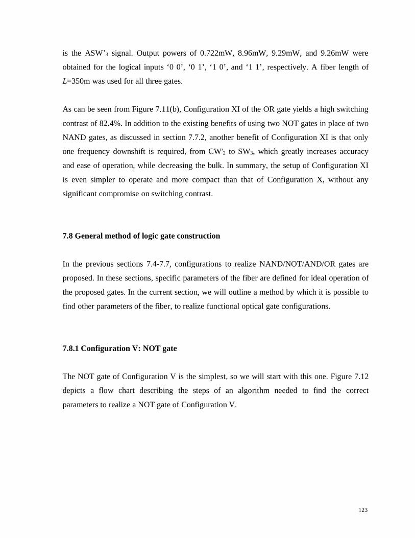
123
is the ASW’3 signal. Output powers of 0.722mW, 8.96mW, 9.29mW, and 9.26mW were
obtained for the logical inputs ‘0 0’, ‘0 1’, ‘1 0’, and ‘1 1’, respectively. A fiber length of
L=350m was used for all three gates.
As can be seen from Figure 7.11(b), Configuration XI of the OR gate yields a high switching
contrast of 82.4%. In addition to the existing benefits of using two NOT gates in place of two
NAND gates, as discussed in section 7.7.2, another benefit of Configuration XI is that only
one frequency downshift is required, from CW'2 to SW3, which greatly increases accuracy
and ease of operation, while decreasing the bulk. In summary, the setup of Configuration XI
is even simpler to operate and more compact than that of Configuration X, without any
significant compromise on switching contrast.
7.8 General method of logic gate construction
In the previous sections 7.4-7.7, configurations to realize NAND/NOT/AND/OR gates are
proposed. In these sections, specific parameters of the fiber are defined for ideal operation of
the proposed gates. In the current section, we will outline a method by which it is possible to
find other parameters of the fiber, to realize functional optical gate configurations.
7.8.1 Configuration V: NOT gate
The NOT gate of Configuration V is the simplest, so we will start with this one. Figure 7.12
depicts a flow chart describing the steps of an algorithm needed to find the correct
parameters to realize a NOT gate of Configuration V.
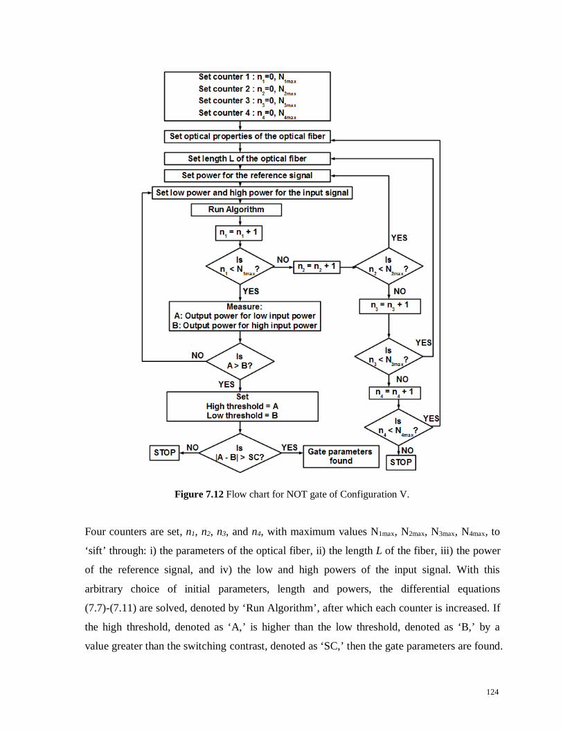
124
Figure 7.12 Flow chart for NOT gate of Configuration V.
Four counters are set, n1, n2, n3, and n4, with maximum values N1max, N2max, N3max, N4max, to
‘sift’ through: i) the parameters of the optical fiber, ii) the length L of the fiber, iii) the power
of the reference signal, and iv) the low and high powers of the input signal. With this
arbitrary choice of initial parameters, length and powers, the differential equations
(7.7)-(7.11) are solved, denoted by ‘Run Algorithm’, after which each counter is increased. If
the high threshold, denoted as ‘A,’ is higher than the low threshold, denoted as ‘B,’ by a
value greater than the switching contrast, denoted as ‘SC,’ then the gate parameters are found.

125
If not, the algorithm is repeated with a different combination of fiber parameters, length and
powers until the correct gate parameters are found.
7.8.2 Configuration IV: NOT gate
For the slightly more complex setup of the NOT gate of Configuration IV, we have the flow
chart of Figure 7.13.
Figure 7.13 Flow chart for NOT gate of Configuration IV.

126
For the algorithm of the NOT gate of Configuration IV, an additional counter is added, n5,
with maximum N5max, to take into account the power of the second reference signal. The rest
of the algorithm remains unchanged.
7.8.3 Configurations I and II: NAND gates
For the NAND gates of Configurations I and II, which do not have frequency detuning, we
have the following flow chart, shown in Figure 7.14 below.
Figure 7.14. Flow chart for NAND gate of Configurations I and II.

127
For the algorithm of the NAND gates of Configurations I-II, the additional counter added, n5,
is used to take into account the second low power and second high power of the second input
signal. ‘C,’ ‘D,’ ‘E,’ and ‘F’ are denoted as the output powers for the effective input
combinations of ‘0 0,’ ‘0 1,’ ‘1 0,’ and ‘1 1’, which are simulated by the combination of low
power and second low power, low power and second high power, high power and second
low power, and high power and second high power. For the NAND gate, for which the
corresponding outputs should be ‘1,’ ‘1,’ ‘1,’ and ‘0’ respectively, C, D, E are evaluated in
comparison to F. If C, D, E > F by a value greater than the switching contrast, ‘SC,’ then the
smallest of C, D, E are set as the high threshold, and F is set as the low threshold. Otherwise,
the counters are increased and the algorithm continues to ‘sift’ through other parameters of
the fiber.
7.8.4 Configuration III: NAND gate
For the NAND gate of Configuration III, which has frequency detuning, we have the
following flow chart, shown in Figure 7.15 below.

128
Figure 7.15 Flow chart for NAND gate of Configuration III.
In the algorithm of the NAND gate of Configuration III, an additional counter is added, n6,
with maximum N6max, to take into account the detuning of the Stokes or anti-Stokes waves.
The rest of the algorithm remains unchanged as compared to the NAND gates of
Configurations I-II.

129
7.8.5 3D parametric model applications in photonic logic
An additional important application of the 3D parametric model of Chapter 3 is in photonic
logic. In section 7.5.2, the construction of an optical NOT gate of Configuration V, utilizing
the mechanisms of SBS, has been described. To obtain a high switching contrast of 77.6%,
such as the one obtained in section 7.5.2, it is important to find the correct combination of
fiber parameters. The initial Stokes power, PSW, was chosen to be the input signal, and an
output CW power, Ppump-out,was taken to be the output signal of the optical gate. The input
CW power was taken to be the reference signal, and was held constant at Ppump=10mW. An
input power of 0.1mW was assigned a logical value of “0,” while an input power of 10mW
was assigned a logical value of “1.” Output powers of 9.0mW and 1.33mW were obtained
for the logical inputs “0” and “1,” respectively, yielding the switching contrast of 77.6%. In
the configuration described in Section 7.5.2, a SNF-28 fiber was used, of length 350m, and a
1550nm laser.
The Brillouin surface can be used to reconstruct this optical gate for any combination of
parameters, not only for the ones used in Section 7.5.2. For example, it is possible to
reproduce the optical logic gate of Section 7.5.2 for the SMF-28e fiber, 1310nm laser, and
1000m fiber, used in Chapter 3, by referring to the Brillouin surface in Figure 3.3. From
Figure 3.3, it is seen that a reference input CW beam of 10mW corresponds to β3=6.4, hence
all combinations of parameters must be on the parametric curve corresponding to β3=6.4.
Furthermore, the output CW power of Ppump-out=1.33mW, corresponding to the “0” output, in
turn corresponds to β1=0.88. For the parameters taken in this manuscript, this yields an input
Stokes power of PSW=1.4mW. Likewise, the output CW power of P1-out=9.0mW,
corresponding to the “1” output, in turn corresponds to β1=0.002. Again, for the parameters
taken in this manuscript, this yields an input Stokes power of PSW=0.003mW. Hence, just by
looking at the Brillouin surface in Figure 3.3, it is possible to find the combination of
parameters of the fiber, to re-create the optical logic gate described in section 7.5.2. Of
course, the 3D parametric model may also be used to construct an optical gate with a higher
switching contrast than the one disclosed in section 7.5.2, or for different, more practical,
input powers.
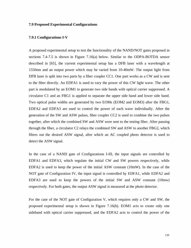
130
7.9 Proposed Experimental Configurations
7.9.1 Configurations I-V
A proposed experimental setup to test the functionality of the NAND/NOT gates proposed in
sections 7.4-7.5 is shown in Figure 7.16(a) below. Similar to the ODPA-BOTDA sensor
described in [65], the current experimental setup has a DFB laser with a wavelength at
1550nm and an output power which may be varied from 10-40mW. The output light from
DFB laser is split into two parts by a fiber coupler CC1. One part works as a CW and is sent
to the fiber directly. An EDFA1 is used to vary the power of this CW light wave. The other
part is modulated by an EOM1 to generate two side bands with optical carrier suppressed. A
circulator C1 and an FBG1 is applied to separate the upper side band and lower side band.
Two optical pulse widths are generated by two EOMs (EOM2 and EOM3) after the FBG1,
EDFA2 and EDFA3 are used to control the power of each wave individually. After the
generation of the SW and ASW pulses, fiber coupler CC2 is used to combine the two pulses
together, after which the combined SW and ASW were sent to the testing fiber. After passing
through the fiber, a circulator C2 relays the combined SW and ASW to another FBG2, which
filters out the desired ASW signal, after which an AC coupled photo detector is used to
detect the ASW signal.
In the case of a NAND gate of Configurations I-III, the input signals are controlled by
EDFA1 and EDFA3, which regulate the initial CW and SW powers respectively, while
EDFA2 is used to keep the power of the initial ASW constant (10mW). In the case of the
NOT gate of Configuration IV, the input signal is controlled by EDFA1, while EDFA2 and
EDFA3 are used to keep the powers of the initial SW and ASW constant (10mw)
respectively. For both gates, the output ASW signal is measured at the photo detector.
For the case of the NOT gate of Configuration V, which requires only a CW and SW, the
proposed experimental setup is shown in Figure 7.16(b). EOM1 acts to create only one
sideband with optical carrier suppressed, and the EDFA2 acts to control the power of the

131
resulting SW. In this case, circulator C2 is moved to the opposite end of the optical fiber, and
the output CW wave is measured by the photo detector.
(a)
(b)
Figure 7.16 NOT experimental setup for test of NAND/NOT gates.
(a) Configurations I-IV, (b) Configuration V.
DFB: Distributed Feedback, RF: radio frequency, C: circulator, CC: fiber coupler,
FUT: fiber under test, I: isolator, EOM: Electro-Optic Modulator, FBG: Fiber Bragg Grating,
PC: polarization controller, EDFA: Erbium-doped fiber amplifier, DAQ: Data Acquisition.

132
7.9.2 Configurations VI
In the current configuration, an AND gate is constructed by connecting the NAND gate of
Configuration III with the NOT gate of Configuration IV, shown in Figure 7.17 below.
Similar to Figure 7.16, the signal from the DFB laser is split by circulator C1 into a SW and
ASW via FBG1, while EOM2 and EOM3 detune the SW and ASW signals individually. In
this case, before the two waves are recombined, couplers CC4 and CC5 redirect the SW and
ASW, to later act as reference signals for the NOT gate. EDFA5 and EDFA4 are used to
control the power of the redirected SW and ASW waves respectively, keeping them constant
(10mW). The NAND gate is represented by the first fiber under test (FUT1). The output
ASW from FUT1, P3-out, after being separated from its output SW counterpart by FBG3, is
passed through a ring resonator RR1 which is utilized to downshift the frequency of the
ASW from ω3 to ω1, which is the frequency of the CW. The resulting converted CW wave
acts as an input signal for the NOT gate, represented by FUT2. Reference signals ASW and
SW are recombined by coupler CC6 and injected into FUT2 from the opposite end, and as
previously, the output ASW is filtered by FBG4 before being measured by the photo
detector.
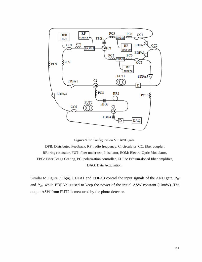
133
Figure 7.17 Configuration VI: AND gate.
DFB: Distributed Feedback, RF: radio frequency, C: circulator, CC: fiber coupler,
RR: ring resonator, FUT: fiber under test, I: isolator, EOM: Electro-Optic Modulator,
FBG: Fiber Bragg Grating, PC: polarization controller, EDFA: Erbium-doped fiber amplifier,
DAQ: Data Acquisition.
Similar to Figure 7.16(a), EDFA1 and EDFA3 control the input signals of the AND gate, P10
and P20, while EDFA2 is used to keep the power of the initial ASW constant (10mW). The
output ASW from FUT2 is measured by the photo detector.

134
7.9.3 Configurations VII
In the current configuration, an AND gate is constructed by connecting the NAND gate of
Configuration III with the NOT gate of Configuration V, shown in Figure 7.18 below. The
dotted lines represent extension to the experimental setup of Figure 7.16(a).
Figure 7.18 Configuration VII: AND gate.
DFB: Distributed Feedback, RF: radio frequency, C: circulator, CC: fiber coupler,
RR: ring resonator, FUT: fiber under test, I: isolator, EOM: Electro-Optic Modulator,
FBG: Fiber Bragg Grating, PC: polarization controller, EDFA: Erbium-doped fiber amplifier,
DAQ: Data Acquisition.
In this configuration, the output ASW, P3-out, after being filtered by FBG3, is passed through
a ring resonator RR1, which downshifts the frequency of the optical signal from ω3 to ω2,
which is the frequency of the SW. The resulting converted SW wave acts as an input signal
for the NOT gate, represented by FUT2. A CW reference signal is injected into FUT2 from
the opposite end. The output CW signal from FUT2 is measured by the photo detector.
In this case, EDFA1 and EDFA3 (Figure 7.16(a)) are used to regulate the input signals of the
AND gate, P10 and P20, while the output CW from FUT2 is measured by the photodetector.
135
7.9.4 Configurations IX
To create a functional OR gate of Configuration IX, three NAND gates from Configuration
III must be connected, shown in Figure 7.19 below. In this case, FUT1, FUT2 and FUT3
represent the three NAND gates, NAND1, NAND2 and NAND3 respectively. In this case,
both inputs to NAND1 and NAND2 are identical. For this reason, the power of the CW and
SW signals, which is controlled by attenuators EDFA1 and EDFA3, for NAND1, and
EDFA7 and EDFA8, for NAND2, must be made identical. Similar to Figure 7.17, before the
generated SW and ASW are recombined by a coupler CC2, another coupler CC4 is used
redirect the ASW, to later act as reference signals for the NAND3. The output ASW from
NAND1 is passed through ring resonator RR1, which downshifts its frequency from ω3 to ω1,
which is the frequency of the CW. The resulting converted CW wave acts as an input signal
for NAND3. The output ASW from NAND2 is passed through ring resonator RR2, which
downshifts its frequency from ω3 to ω2, which is the frequency of the SW. The resulting
converted SW wave acts as the second input signal for NAND3, and is injected into FUT3 at
the opposite end, after being recombined with the redirected ASW by coupler CC7. The
output ASW signal from FUT3 from is then filtered by FBG4 and measured by the photo
detector.

136
Figure 7.19 Configuration IX: OR gate.
DFB: Distributed Feedback, RF: radio frequency, C: circulator, CC: fiber coupler,
RR: ring resonator, FUT: fiber under test, I: isolator, EOM: Electro-Optic Modulator,
FBG: Fiber Bragg Grating, PC: polarization controller, EDFA: Erbium-doped fiber amplifier,
DAQ: Data Acquisition.
In this case, EDFA1 and EDFA3, and EDFA7 and EDFA8, are used to regulate the input
signals of the AND gate, while the output ASW from FUT3 is measured by the photo
detector.
The same detuning must be applied to optical signals entering FUT1 (NAND gate 1), FUT2
(NAND gate 2) and FUT3 (NAND gate 3), as described in Table 3 of Configuration III. To

137
accomplish this, combined SW and ASW signals by coupler CC2 are split by coupler CC9
into two paths, one path is injected into FUT1, while the SW and ASW signals on the second
path are split by circulator C5 and separated by FBG6. In this way, it is possible to detune the
SW and ASW separately by EOM4 and EOM5, such that the resulting recombined signals by
coupler CC8 are detuned accordingly, before being injected into FUT2.
7.9.5 Configurations X
The setup to create a functional OR gate of Configuration X is very similar to that of
Configuration IX depicted in Figure 7.19. The difference is that two NOT gates of
Configuration IV and one NAND gate from Configuration III must be connected. Keeping
this difference in mind, it follows that FUT1 and FUT2 represent the two NOT gates, NOT1
and NOT2 respectively, and FUT3 represents the NAND gate, NAND3 respectively. In this
case, only one input to NOT1 and NOT2 exist, which are the CW signals controlled by
attenuators EDFA1 for NOT1 and EDFA8 for NOT2. The ASW and SW reference signals,
which are controlled respectively by attenuators EDFA2 and EDFA3 for NOT1, and EDFA6
and EDFA7 for NOT2, are kept constant at 10mW. Similar to Figure 7.17, before the
generated SW and ASW are recombined by a coupler CC2, another coupler CC4 is used
redirect the ASW, to later act as reference signals for the NAND3. The output ASW from
NOT1 is passed through ring resonator RR1, which downshifts its frequency from ω3 to ω1,
which is the frequency of the CW. The resulting converted CW wave acts as an input signal
for NAND3. The output ASW from NOT2 is passed through ring resonator RR2, which
downshifts its frequency from ω3 to ω2, which is the frequency of the SW. The resulting
converted SW wave acts as the second input signal for NAND3, and is injected into FUT3 at
the opposite end, after being recombined with the redirected ASW by coupler CC7. The
output ASW signal from FUT3 from is then filtered by FBG4 and measured by the photo
detector.

138
7.9.6 Configurations XI
The setup to create a functional OR gate of Configuration XI is comprised of two NOT gates
of Configuration V and one NAND gate from Configuration III. To realize this setup, the
experimental setups from Figure 7.16(b) must be combined with the experimental setup of
7.16(a), shown below in Figure 7.20. In this case, FUT1 and FUT2 represent the two NOT
gates, NOT1 and NOT2 respectively, and FUT3 represents the NAND gate, NAND3
respectively. In this case, only one input to NOT1 and NOT2 exist, which are the SW signals
controlled by attenuators EDFA3 for NOT1 and EDFA7 for NOT2. The CW reference
signals, which are controlled respectively by attenuators EDFA1 for NOT1, and EDFA8
NOT2, are kept constant at 10mW. Since the NOT gates in this setup are 2-wave NOT gates,
the SW and ASW waves are no longer recombined by a coupler CC2, the ASW is simply
redirected to later act as a reference signal for the NAND3. The output CW from NOT1 is
passed directly to the FUT3, the redirected CW wave acts as an input signal for NAND3. The
output CW from NOT2 is passed through ring resonator RR1, which downshifts its
frequency from ω1 to ω2, which is the frequency of the SW. The resulting converted SW
wave acts as the second input signal for NAND3, and is injected into FUT3 at the opposite
end, after being recombined with the redirected ASW by coupler CC7. The output ASW
signal from FUT3 from is then filtered by FBG4 and measured by the photo detector.

139
Figure 7.20 Configuration XI: OR gate.
DFB: Distributed Feedback, RF: radio frequency, C: circulator, CC: fiber coupler,
RR: ring resonator, FUT: fiber under test, I: isolator, EOM: Electro-Optic Modulator,
FBG: Fiber Bragg Grating, PC: polarization controller, EDFA: Erbium-doped fiber amplifier,
DAQ: Data Acquisition.
In this case, EDFA3 and EDFA7, are used to regulate the input signals of the AND gate,
while the output ASW from FUT3 is measured by the photo detector.

140
7.10 Bit rate
Because optical gates based on the process of SBS, or combined Brillouin gain and loss, are
limited by a phonon relaxation time of about 10ns, and because of the narrowband
characteristic of Brillouin amplification, the bit rate of the Brillouin signal is limited to tens
of megabits per second [101, 102]. However, there are a number of techniques aimed at
increasing the Brillouin gain bandwidth, thereby supporting a higher bit rate. These include a
simple pump-spectral broadening technique [103, 104] via direct- modulation of the pump
laser using a pseudorandom binary sequence (PRBS) data, a Gaussian noise source.
Alternatively, the pump wave can be broadened by using an external phase modulator (PM),
which has been demonstrated to yield bit rates between 1-2.5 Gb/s [101, 105]. Comparatively,
bit rates between 10 Gb/s to 100 Gb/s have been claimed by other technologies to construct
optical logic units [37, 43, 49, 51, 106, 107]. Though these alternative constructions have
higher bit rates, they also include numerous drawbacks, including configurations which are
both bulky and require extensive calibration, and fall victim to spontaneous emission noise,
time dependent modulation due to time jitter, and birefringence induced signal distortion.
The technique based on combined Brillouin gain and loss, disclosed in this chapter, is free of
polarization-induced signal fluctuations which cause spectral distortion, thereby making the
lower bit rate a worthy trade-off.
7.11 Summary
A novel fiber nonlinearity-based technique has been proposed to realize all-optical
NAND/NOT/AND/OR logic gates, based on the principles of combined Brillouin gain and
loss in a PMF. Switching contrasts are simulated to be between 20-83%, for various
configurations. In addition, the technique is not limited by polarization instabilities or PMD.
Additionally, a general method for constructing optical gates has been proposed in the form
of an algorithm.
Finally, experimental configurations have been proposed to realize the optical logic gates of
Configurations I-XI.

141
Chapter 8
Conclusion
8.1 Thesis Outcomes
The main focus of the research presented in this thesis was on the theoretical investigation of
stimulated Brillouin scattering (SBS), as well as combined Brillouin gain and loss, in optical
fibers and their application to current technologies in fiber sensing, photonic logic, and
telecommunications.
Experimentally verified fully analytic expressions have been obtained for the Brillouin
amplification process without any underlying assumptions about the behaviour of the pump
or pulse waves. Additionally, for the first time, analytic solutions for the output pump and
Stokes spectra have been obtained to good accuracy, as well as an expression for the FWHM,
which have been confirmed experimentally. In sensing applications, the 3D parametric
model may be used to avoid parameter combinations which yield the unwanted spectral
distortion effect, such as in distributed sensing where pump depletion is substantial. The 3D
parametric model can also be used to classify the similarity between various Brillouin
amplification processes, making it possible to obtain the same pump or Stokes output
intensity with a different collection of parameters of the fiber. This, in particular, has useful
applications in the construction of all-optical logic gates.
Regarding applications in telecommunications, the SBS process has been used to develop an
improved method of phase-modulation, and applied in the conceptualization of an optical
phase-modulator based on the principles of SBS, as well as an optical phase network
employing the same.
Polarization and birefringence effects on SBS, and combined Brillouin gain and loss, in an
optical fiber have been investigated. The most general model of elliptical birefringence in an

142
optical fiber has been developed and extended to describe a transient Brillouin interaction
including gain, loss, and combined gain and loss. The subsequent investigation of SBS
spectral distortion effects, caused by the birefringence and polarization of the optical fiber,
showed that these effects can be used for measuring the degree of non-ideally linearly
polarized light, finding regimes which are preferable for measurement in fiber sensing, and
for preserving the full width at half maximum (FWHM) and pulse fidelity of the Brillouin
spectral shape, which has applications in telecommunications and data transmission. In the
combined Brillouin gain and loss regime, it has been shown that the spectral distortion
caused by birefringence can be minimized by choosing pump and pulse powers with a large
disparity, thereby increasing the ease of operation of the optical differential parametric
amplification in optical differential parametric amplification (ODPA-BOTDA) systems.
Finally, the theory of combined Brillouin gain and loss has been employed to propose a novel
fiber nonlinearity-based technique to realize all-optical NAND/NOT/AND/OR logic gates in
polarization-maintaining fibers (PMF). Switching contrasts are simulated to be between
20-83% for various configurations. In addition, the technique is not limited by polarization
instabilities or PMD. Finally, experimental configurations have been proposed to realize the
optical logic gates.
8.2 Future Work
Future research directions could include the experimental verification of the theoretical
works presented in this thesis. Namely, experimental confirmation of the optical
phase-modulator of Chapter 4, as well as the optical network employing the optical
phase-modulator, would be a logical next step in the development of this technology.
For the all-optical logic gates proposed in Chapter 7, an interesting avenue for research could
include the use of chalcogenide fibers in place of silica fibers to realize the all-optical gates.
Chalcogenide fibers are characterized by pronounced optical nonlinearities. Compared to
silica, for example, the nonlinear refractive index of As2S3 glass is about 1000 larger [61, 108,

143
109, 110, 111, 112], and the Brillouin gain coefficient was reported to be between 100-600
times larger than in fused silica [108, 111]. As a result, a comparable gain may be
accomplished in chalcogenide fibers of a few meters as compared to silica fibers of hundreds
of meters, which would greatly compactify the setups described in Chapter 7. Additionally,
the 3D parametric model may be used to characterize this new chalcogenide optical gate, as
described in section 7.8.5. Furthermore, realization of the experimental configurations
proposed in section 7.9, as well as performing multiple-gate connections, would be an
important next step in the development of the photonic logic technology.
Regarding the theoretical investigation of polarization and birefringence effects, additional
studies could be performed to investigate the effects of a non-uniform fiber on spatial
resolution, by simulating different sound velocities for different segments of the optical fiber.
Additionally, it would also be interesting to see the spectral evolution as a function of
coordinate inside the optical fiber, z. It has been shown experimentally [113] that a spectral
"oscillation" occurs inside the fiber; future work could include modeling this behaviour
theoretically and seeing how the spatial period of these oscillations is related to the PMD and
beat length of the fiber. Additionally, experimental verification of the current theory could be
performed by inducing elliptical birefringence in a PMF fiber by twisting it in a controlled
way and performing measurements on the twisted fiber.

144
Bibliography
[1] R. Boyd, Nonlinear Optics, second ed., Academic Press, New York, 1992.
[2] P. Bayvel, P.M. Radmore, "Solutions of the SBS equations in single mode opticalfibers and implications for fibre transmission systems," Electronics Letters 26, 434-436(1990).
[3] E. Geinitz, S. Jetschke, U. Röpke, S. Schröter, R. Willsch and H. Bartelt, "Theinfluence of pulse amplification on distributed fibre-optic Brillouin sensing and a methodto compensate for systematic errors," Measurement Science and Technology 10, 112-116(1999).
[4] X. Bao, L. Chen, "Recent Progress in Distributed Fiber Optic Sensors," Sensors 12,8601-8639 (2012).
[5] S. L. Zhang, J. J. O’Reilly, "Effect of Stimulated Brillouin Scattering on DistributedErbium-Doped Fiber Amplifier," IEEE Photonics Techonology Letters 5, 537-539 (1993).
[6] B. Foley, M. L. Dakss, R. W. Davies, P. Melman, "Gain Saturation in Fiber RamanAmplifiers Due to Stimulated Brillouin Scattering," J. of Lightwave Technology 7,2024-2032 (1989)
[7] F. S. Gokhan, "Moderate-gain Brillouin amplification: An analytical solution belowpump threshold," Optics Communications 284, 4869-4873 (2011).
[8] C. L. Tang, "Saturation and Spectral Characteristics of the Stokes Emission in theStimulated Brillouin Process," J. of Applied Physics 37, 2945-2955 (1966).
[9] L. Chen, X. Bao, "Analytical and Numerical Solutions for Steady State StimulatedBrillouin Scattering in a Single-mode Fiber," Optics Communications 152, 65-70 1998).
[10] A. Kobyakov, S. Darmanyan, M. Sauer, D. Chowdhury, "High-gain Brillouinamplification: an analytical approach," Optics Letters 31, 1960-1962 (2006).
[11] A. Chen, E. Murphy, Broadband Optical Modulators: Science, Technology, andApplications, first ed., CRC Press, Boca Raton, 2012.
[12] R. Hui, M. O'Sullivan, Fiber Optic Measurement Techniques, first ed., ElsevierAcademic Press, Burlington, 2009.
[13] M. M. Rao, Optical Communication, first ed., Universal Press, Hyderguda, 2000.
[14] J. N. Downing, Fiber-optic Communications, first ed., Thomson Delmar Learning,Clifton Park, 2005.
[15] C. DeCusatis, I. P. Kaminow, The Optical Communications Reference, first ed.,

145
Academic Press, Oxford, 2010.
[16] P. E. Powers, Fundamentals of Nonlinear Optics, first ed., CRC Press, Boca Raton,2011.
[17] Y. S. Kuz'minov, Lithium Niobate Crystals, first ed., Cambridge InternationalScience Publishing, Cambridge, 1999.
[18] R. Hui, Q. Jiang, M. Kavehrad, T. Makino, “All-optical phase modulation in atraveling wave semiconductor laser amplifier”, IEEE Photonics Technology Letters 6,808-810 (1994).
[19] D. R. Walker, M. Bashkanski, A. Gulian, F. K. Fatemi, M. Steiner, "Stabilizing slowlight delay in stimulated Brillouin scattering using a Faraday rotator mirror," JOSA B 25,C61-C64 (2008).
[20] L. Thevenaz, "Slow and Fast Light in Optical fibers,"Nature Photonics 2, 474-481(2008).
[21] G. M. Gehring, R. W. Boyd, A. L. Gaeta, D. J. Gauthier, A. E. Willner, "Fiber-basedSlow-Light Technologies," J. of Lightwave Technology 26, 3752-3762 (2008).
[22] R. H. Stolen, "Polarization Effects in Fiber Raman and Brillouin Lasers," J. ofQuantum Electronics QE-15, 1157-1160 (1979).
[23] O. Shlomovits, M. Tur, "Vector analysis of depleted stimulated Brillouin scatteringamplification in standard single-mode fibers with non-zero birefringence," Optics Letters38, 836-838 (2013).
[24] L. Ursini, M. Santagiustina, L. Palmieri, "Polarization-Dependent Brillouin Gain inRandomly Birefringence Fibers," IEEE Photonics Technology Letters 22, 712-714(2010).
[25] M. Oskar van Deventer, A. J. Boot, "Polarization Properties of Stimulated BrillouinScattering in Single-Mode Fibers," J. of Lightwave Technology 12, 585-590 (1994).
[26] W. Zou, Z. He, K. Hotate, "Complete discrimination of strain and temperature usingBrillouin frequency shift and birefringence in a polarization-maintaining fiber," OpticsExpress 17, 1248-1255 (2009).
[27] A. Zadok, A. Eyal, M. Tur, "Polarization attributes of stimulated Brillouin scatteringslow light in fiber," Proc. of SPIE 7949, 79490A (2011).
[28] S. Xie, M. Pang, X. Bao, L. Chen, “Polarization dependence of Brillouin linewidthand peak frequency due to fiber inhomogeneity in single mode fiber and its impact ondistributed fiber Brillouin sensing,” Opt Express 20, 6385-6399 (2012) .
[29] L. Thevenaz, M. Facchini, A. Fellay, M. Nikles, P. Robert, "Evaluation of local

146
birefringence along fibres using Brillouin analysis," Optical Fibre MeasurementConference OFMC'97,82-85 (1997).
[30] A. Zadok, S. Chin, L. Thevenaz, E. Zilka, A. Eyal, M. Tur, "Polarization-induceddistortion in stimulated Brillouin scattering slow-light systems," Optics Letters 34,2530-2532 (2009).
[31] T. Chattopadhyay, “Optical programmable Boolean logic unit,” Applied Optics 52,6049-6056 (2011).
[32] T. Chattopadhyay, “Optical reversible programmable Boolean logic unit,” AppliedOptics 51, 5266-5271 (2012).
[33] M. R. Fetterman, "Design for high-speed optoelectronic Boolean logic," IEEEPhotonics Technology Letters 21, 1740-1742 (2009).
[34] J. Yang, X. Li, J. Yang, J. Liu, X. Su, "Polarization-independent bidirectional 4 x 4optical switch in free-space," Optical Laser Technology 43, 927-933 (2010).
[35] Y. Wu, T. Shih, M. Chen, “New all-optical logic gates based on the local nonlinearMach-Zehnder interferometer,” Optics Express 16, 248-257 (2008).
[36] M. Nazari, M. Haghparast, “Novel design of all-optical reversible logic gate usingMach-Zehnder interferometer in the field of nanotechnology,” Australian J. of Basic andApplied Science 5, 923-929 (2011).
[37] T. Chattopadhyay, “All-optical modified Fredkin gate,” IEEE J. of Selected Topics inQuantum Electronics 18, 585-592 (2012).
[38] Z. Li, G. Li, “Ultrahigh speed reconfigurable logic gates based on four-wave mixingin a semiconductor optical amplifier,” Photonics Technology Letters 18, 1341-1343(2006).
[39] S. H. Kim, J. H. Kim, B. G. Yu, Y. T. Byun, Y. M. Jeon, S. Lee, D. H. Woo, S. H.Kim, “All-optical NAND gate using cross-gain modulation in semiconductor opticalamplifiers,” Electronics Letters 41, 1027-1028 (2005).
[40] D. Nesset, T. Kelly, D. Marcenac, "All-optical wavelength conversion using SOAnonlinearities," IEEE Communications Magazine 36, 56-61 (1998).
[41] C. Schubert, R. Ludwig, H-G. Weber, “High-speed optical signal processing usingsemiconductor optical amplifiers," J. of Optical and Fiber Communication ResearchReports 2, 171-208 (2004).
[42] X. Ye, P. Ye, M. Zhang, “All-optical NAND gate using integrated SOA-basedMach-Zehnder interferometer,” Optical Fiber Technology 12, 312-316 (2006).

147
[43] T. Chattopadhyay, “All-optical programmable Boolean logic unit using SOA-MZIswitch,” IET Optoelectronics 5, 270-280 (2011).
[44] K. I. Kang, T.G. Chang, I. Glesk, P. R. Prucnal, "Comparison of Sagnac andMach-Zehnder ultrafast all-optical interferometric switches based on semiconductorresonant optical nonlinearity," Applied Optics 35, 417-426 (1996).
[45] J. Y. Kim, J. M. Kang, T. Y. Kim, S. K. Han, "All-optical multiple logic gates withXOR, NOR, OR and NAND functions using parallel SOA-MZI structures: theory andexperiment," J. of Lightwave Technology 24, 3392-3399 (2006).
[46] J. Wang, J. Sun, Q. Sun, “Experimental observation of a 1.5μm band wavelengthconversion and logic NOT gate at 40 Gbit/s based on sum-frequency generation,” OpticsLetters 31, 1711-1713 (2006).
[47] J. Wang, J. Sun, Q. Sun, “Proposal for all-optical switchable OR/XOR logic gatesusing sum-frequency generation,” IEEE Photonics Technology Letters 19, 541-543(2007).
[48] Z. Y. Shen, L. L.Wu, “Reconfigurable optical logic unit with terahertz opticalasymmetric demultiplexer and electro optic switches,” Applied Optics 47, 3737-3742(2008).
[49] T. Chattopadhyay, “Eliminating the additional input beam in all-optical XOR gateusing Terahertz Optical Asymmetric Demultiplexer (TOAD) based interferometer: Atheoretical analysis,” Optik International J. for Light and Electron Optics 122, 1486–1491(2011).
[50] T. Chattopadhyay, “All-optical terahertz optical asymmetric demultiplexer (TOAD)based binary comparator: a proposal,” J. of Nonlinear Optical Physics & Materials 18,471-480 (2009).
[51] T. Chattopadhyay, “All-optical cross-bar network architecture using TOAD basedinterferometric switch and using it to design reconfigurable logic unit,” Optical FiberTechnology 17, 558-567 (2011).
[52] A. W. Lohmann, “Polarization and optical logic,” Applied Optics 25, 1594-1597(1986).
[53] M. A. Karim, A. A. S. Awwal, A. K. Cherri, “Polarization-Encoded OpticalShadow-Casting Logic Units: Design,” Applied Optics 26, 2720-2725 (1987).
[54] T. Chattopadhyay, T. Sarkar, “All-optical by Kerr nonlinear prism and its applicationto of binary-to-gray-to-binary code conversion,” Optics & Laser Technology 44,1722-1728 (2012).
148
[55] C. Yu, L. Christen, T. Luo, Y. Wang, Z. Pan, L. Yan, A. E. Willner, “All-optical XORgate using polarization rotation in single highly nonlinear fiber,” Photonics TechnologyLetters 17, 1232-1234 (2005).
[56] C. Yu, L. Christen, T. Luo, Y. Wang, Z. Pan, L. Yan, A. E. Willner, “All-optical XORgate based on Kerr effect in single highly-nonlinear fiber,” Proc. of Conf. Lasers andElectro-Optics (CLEO), 3-5 (2004).
[57] K. Suzuki, H. Kubota, S. Kawanishi, M. Tanaka, M. Fujita, “Optical properties oflow-loss polarization-maintaining photonic crystal fiber,” Optics Express 9, 676-680(2001).
[58] T. Hosaka, K. Okamoto, T. Miya, Y. Sasaki, T. Edahiro, “Low-loss singlepolarization fibers with asymmetrical strain birefringence,” Electronics Letters 17,530-531 (1981).
[59] R. D. Birch, D. N. Payne, M. P. Varnham, “Fabrication of polarization-maintainingfibers using gas-phase etching,” Electronics Letters 18, 1036-1038 (1982).
[60] J. D. Jackson, Classical Electrodynamics, first ed., John Wiley & Sons, Inc., NewYork, 1962.
[61] G. P. Agrawal, Nonlinear Fiber Optics, third ed., Academic Press, San Diego, 2001.
[62] A. B. Ruffin, "Stimulated Brillouin Scattering: An overview of measurements,system impairments, and applications," NIST Symposium on Optical FiberMeasurements 2, 23-28 (2004).
[63] A. Kobyakov, M. Sauer, D. Chowdhury, “Stimulated Brillouin scattering in opticalfibers,” Advances in Optics and Photonics 2, 1-59 (2010).
[64] I. L. Fabelinskii, Molecular Scattering of Light, first ed., Plenum Press, Moscow,1968.
[65] Y. Li, X. Bao, Y. Dong, L. Chen, "A novel distributed Brillouin sensor based onoptical differential parametric amplification," J. Lightwave Technology 28, 2621–2626(2010).
[66] E. Collette, Field Guide to Polarization, first ed., SPIE Press, Washington, 2005.
[67] A. Kumar, A. Ghatak, Polarization of Light with Applications in Optical Fibers, firsted., SPIE press, Washington, 2011.
[68] E. Collette, Polarized Light in Fiber Optics, first ed., The PolaWave Group, Lincroft,2003.
149
[69] A. Rogers, Polarization in Optical Fibers, first ed., Artech House Inc., Norwood,2008.
[70] F. Ravet, Performance of the Distributed Brillouin Sensor: Benefits and PenaltiesDue to Pump Depletion, first ed., University of Ottawa Press, Ottawa, 2007.
[71] T. Horiguchi, K. Shimizu, T. Kurashima, M. Tateda, Y. Koyamada, "Development ofa distributed sensing technique using Brillouin scattering," J. of Lightwave Technology13, 1296-1302 (1995).
[72] L. Thévenaz, S. F. Mafang, "Depletion in a distributed Brillouin fiber sensor:practical limitation and strategy to avoid it," J. Lin. Proc. of SPIE 7753A5 1-4 (2011).
[73] A. Minardo, R. Bernini, L. Zeni, L. Thevenaz, F. Briffod, "A reconstructiontechnique for long-range stimulated Brillouin scattering distributed fibre-optic sensors:experimental results," Measurement Science and Technology 16, 900-908 (2005).
[74] T. H. Russell, W. B. Roh, "Threshold of second-order stimulated Brillouin scatteringin optical fiber," JOSA B 19, 2341-2345 (2002).
[75] J. W. D. Chi, L. Chao, M. K. Rao, "Time-domain large-signal investigation onnonlinear interactions between an optical pulse and semiconductor waveguides," J. ofQuantum Electronics 37, 1329-1336 (2001).
[76] R. Chu, M. Kanefsky, J. Falk, "Numerical study of transient stimulated Brilllouinscattering," J. of Applied Physics 71, 4653 - 4658 (1992).
[77] M. Razaghi, V. Ahmadi, M. J. Connelly, "Comprehensive Finite-DifferenceTime-Dependent Beam Propagation Model of Counterpropagating Picosecond Pulses in aSemiconductor Optical Amplifier," J. of Lightwave Technology 27, 3162-3174 (2009).
[78] F. S. Gokhan, G. W. Griffiths, W. E. Schiesser, "Method of lines solution to thetransient SBS equations for nanosecond Stokes pulses," J. of the European OpticalSociety 8, 13049 (2013).
[79] Z. Zhu, D. J. Gauthier, Y. Okawachi, J. E. Sharping, A. L. Gaeta, R. W. Boyd, A. E.Willner, "Numerical study of all-optical slow-light delays via stimulated Brillouinscattering in an optical fiber," JOSA B 22, 2378-2384 (2005).
[80] C. Zeringue, I. Dajani, S. Naderi, G. T. Moore, C. Robin, "A theoretical study oftransient stimulated Brillouin scattering in optical fibers seeded with phase-modulatedlight," Optics Express 20, 21196-21213 (2012).
[81] D. Cotter, "Transient Stimulated Brillouin Scattering in long single-mode fibres,"Electronics Letters 18, 504-506 (1982).
[82] V. P. Kalosha, L. Chen, X. Bao, "Slow and fast light via SBS in optical fibers for

150
short pulses and broadband pump," Optics Express 14, 12693-12703 (2006).
[83] V. P. Kalosha, E. A. Ponomarev, L. Chen, X. Bao, "How to obtain high spectralresolution of SBS-based distributed sensing by using nanosecond pulses," Optics Express14, 2071-2077 (2006).
[84] S. V. Afshar, G. A. Ferrier, X. Bao, L. Chen, "Effect of the finite extinction ratio ofan electro-optic modulator on the performance of distributed probe-pump Brillouin sensorsystems," Optics Letters 28, 1418-1420 (2003).
[85] R. Bernini, A. Minardo, L. Zeni, "Dynamic strain measurement in optical fibers bystimulated Brillouin scattering,: Optics Letters 34, 2613-2615 (2009).
[86] X. Bao, C. Zhang, W. Li, M. Eisa, S. El-Gamal, B. Benmokrane, "Monitoring thedistributed impact wave on a concrete slab due to the traffic based on polarizationdependence on stimulated Brillouin scattering," Smart Materials and Structures 17, 1-5(2008).
[87] V. I. Kovalev, R. G. Harrison, "Observation of Inhomogeneous Spectral Broadeningof Stimulated Brillouin Scattering in an Optical Fiber," Physical Review Letters 85,1879-1882 (2000).
[88] L. Stepien, S. Randoux, J. Zemmouri, "Origin of spectral hole burning in Brillouinfiber amplifiers and generators," Physical Review A 65, 053812 (2002).
[89] X. Bao, L. Chen, “Recent Progress in Optical Fiber Sensors based on Brillouinscattering at University of Ottawa,” Photonic Sensors 1, 102-117 (2011).
[90] H. A. Luther, "An Explicit Sixth-Order Runge-Kutta Formula," Mathematics ofComputation 22, 424-436 (1968).
[91] J. C. Butcher, "On Fifth and Sixth Order Explicit Runge-Kutta Methods: OrderConditions and Order Barriers," Canadian Applied Mathematics Quarterly 17, 433-445(2009).
[92] W. Zou, C. Jin, J. Chen, “Distributed Strain Sensing Based on Combination ofBrillouin Gain and Loss Effects in Brillouin Optical Correlation Domain Analysis,”Applied Physics Express 5, 082503 (2012).
[93] K. Y. Song, Z. He, K. Hotate, "Distributed strain measurement with millimeter-orderspatial resolution based on Brillouin optical correlation domain analysis," Optics Letters31, 2526-2528 (2006).
[94] W. Zou, Z. He, M. Kishi, K. Hotate, "Stimulated Brillouin scattering and itsdependences on strain and temperature in a high-delta optical fiber with F-dopeddepressed inner cladding," Optics Letters 32, 600-602 (2007).
[95] A. Kumar, Switching Theory and Logic Design, first ed., PHI Learning Private

151
Limited, New Delhi, 2008.
[96] N. J. Doran, D. Wood, “Nonlinear-optical loop mirror,” Optics Letters 13, 56-58(1988).
[97] S. H. Larsen, M. E. V. Pedersen, L. Gruner-Nielsen, M. F. Yan, E. M. Monberg, P. W.Wisk, K. Rottwitt, “Polarization Maintaining Higher Order Mode Fiber Module withAnomalous Dispersion at 1μm,” Optics Letters 37, 4170-4172 (2012).
[98] M. Tur, E. Herman, A. Kozhekin, Y. Danziger, “Stimulated Brillouin Scattering inHigh-Order Mode fibers employed in dispersion management modules,” IEEE Photon.Technology Letters 14, 1282-1284 (2002).
[99] A. Bogoni, L. Poti, R. Proietti, G. Meloni, F. Ponzini, P. Ghelfi, “Regenerative andreconfigurable all-optical logic gates for ultra-fast applications,” Electronics Letters 41,435-436 (2005).
[100] Y. Miyoshi, R. Ikeda, H. Tobioka, T. Inoue, S. Namiki, K. Kitayama, “Ultrafastall-optical logic gate using a nonlinear optical loop mirror based multi-periodic transferfunction,” Optics Express 16, 2570-2577 (2008).
[101] L. Yi, L. Zhan, W. Hu, Y. Xia, "Delay of Broadband Signals Using Slow Light inStimulated Brillouin Scattering With Phase-Modulated Pump," IEEE PhotonicsTechnology Letters 19, 619-621 (2007).
[102] M. Lee, R. Pant, M. A. Neifeld, "Improved slow-light delay performance of abroadband stimulated Brillouin scattering system using fiber Bragg gratings," AppliedOptics 47, 6404-6415 (2008).
[103] M. G. Herraez, K. Y. Song, L. Thevenaz, “Arbitrary-bandwidth Brillouin slow lightin optical fibers,” Optics Express 14, 395–1400 (2006).
[104] Z. Zhu, A. M. C. Dawes, D. J. Gauthier, L. Zhang, A. E. Willner,"12-GHz-bandwidth SBS slow light in optical fibers,” Proc. OFC PDP1, 1-3 (2006).
[105] L. Yi, L. Zhan, Y. Su, W. Hu, L. Leng, Y. Song, H. Shen, Y. Xia, “Delay of RZPRBS data based on wideband SBS by phase-modulating the Brillouin pump,” Proc.ECOC We3.P.30, 1-2 (2006).
[106] L. Yi, W. Hu, H. He, Y. Dong, Y. Jin, W. Sun, "All-Optical reconfigurablemulti-logic gates based on nonlinear polarization rotation effect in a single SOA,"Chinese Optics Letters 9, 030603-1 - 030603-4. (2011).
[107] J. Yang, L. Han, H. Zhang, Y. Guo, " Function-lock strategy in OR/NOR opticallogic gates based on cross-polarization modulation effect in semiconductor opticalamplifier," Chinese Optics Letters 5, 566-568 (2007).

152
[108] S. Levy, V. Lyubin, M. Klebanov, J. Scheuer, A. Zadok, "Stimulated Brillouinscattering amplification in centimeter-long directly written chalcogenide waveguides,"Optics Letters 37, 5112-5114 (2012).
[109] J. L. Adam, X. Zhang, Chalcogenide Glasses: Preparation, Properties andApplications, first ed., Woodhead Publishing, New Delhi, India, 2014.
[110] J. S. Sanghera, L. B. Shaw, C. M. Florea, P. Pureza, V. Q. Nguyen, F. Kung, D.Gibson, I. D. Aggarwal, "Nonlinear Properties of Chalcogenide glass fibers," J. ofOptoelectronics and Advanced Materials 8, 2148-2155 (2006).
[111] R. Cherif, A. Salem, M. Zghal, "Full modal analysis of the stimulated Brillouinscattering in As2S3 chalcogenide photonic crystal fiber," Proc. Of SPIE 8073, (2011).
[112] J. S. Sanghera, L. B. Shaw, I. D. Aggarwal, "Applications of Chalcogenide glassoptical fibers," Comptes Rendus Chimie 5, 873-883 (2002).
[113] Y. Li, Development of the Distributed Brillouin Sensor with High Spatial andFrequency Resolution, first ed., University of Ottawa Press, Ottawa, 2010.

153
Appendix
A. Derivation of the system of equations (5.1)-(5.4)
Let us consider the simple case of two propagation constants in the fiber, x and y . If a light
with an angular frequency ω was injected into the fiber, the electric fields could be written in
the following form, in terms of their principal axis of polarization
ytzkiExtzkiEtzE yyxx expexp,1 (A.1)
Where yyxx 1 and 0yx . Considering two counter-propagating beams in
the fiber, we can individually write them for the +z-propagating light,
111111111 expexp, ytzkiExtzkiEtzE yyxx (A.2)
And the – z-propagating light,
222222222 expexp, ytzkiExtzkiEtzE yyxx (A.3)
The beating via electrostriction in the fiber due to the two light waves can be written
explicitly
122121
*21
122121*21
122121*21
122121*2112
exp
exp
exp
exp,,
yxtzkkiEE
xytzkkiEE
yytzkkiEE
xxtzkkiEEtzEtzE
xyxy
yxyx
yyyy
xxxx
(A.4)
In the most general case of elliptical birefringence, we will have 1212 1 yyxx and

154
furthermore 1212 0 yxxy . The direct physical consequence of this is that there are
now four acoustic running waves.
Taking the steady state approximation, we have the complex acoustic field amplitude for the
simplest case of zero birefringence, where q=q1≈2k1 as defined in Chapter 2:
tzEtzEi
q
BB
e ,, 121
21
2
2
(A.5)
To generalize the result to the case of elliptical birefringence, where it is expected to have the
corresponding resonance frequency associated with the principal birefringence axes, we
make ΩB to be functions of the polarization principal axis beatings [30], with ΩBxx, ΩByy, ΩBxy
and ΩByx as defined in Chapter 5. Furthermore, the following approximation is used
2
12
12
/
1
11
11
12
121
2
2
BB
e
BB
e
BBB
e
BB
e
icvn
ivq
i
qi
q
(A.6)
as well as the approximation c
nnnc
kkq 21221121 , where n and are
taken to be the averages of n1 and n2, and ω1 and ω2 respectively. It is then possible to have
the following approximate complex acoustic field amplitudes,

155
122121
*21
1
122121*21
1
122121*21
1
122121*21
1
exp
2
1
exp
2
1
exp
2
1
exp
2
1
yxtzkkiEEicv
n
xytzkkiEEicv
n
yytzkkiEEicv
n
xxtzkkiEEicv
n
xyxyB
Byx
e
yxyxB
Bxy
e
yyyyB
Byy
e
xxxxB
Bxx
e
(A.7)
Paying attention to the original case without birefringence in equation (A.5), it is possible to
generalize our result. Recall that non-birefringent lights were assumed to undergo ideal
power transfer between the pump wave and the Stokes wave, as would be the case when both
these waves are parallel-polarized (under the slowly varying amplitudes, A1 and A2,
approximation),
20
11
11
2A
nciA
tA
cn
zA e
(A.8)
1*
0
22
22
2A
nciA
tA
cn
zA e
(A.9)
In equations (A.8) and (A.9), ρ0 is the mean density of the fiber. Generalizing the above
system of equations (A.8) and (A.9) to the case of birefringence we take the following,
21122
*21
110
1
21122*21
110
1
11111
2
12
2
12
yxxyEEEicv
ncn
i
xxxxEEEicv
ncn
i
Et
Ec
nz
E
yyxB
Bxy
e
x
e
xxxB
Bxx
e
x
e
xxxxx
(A.10)

156
21122
*21
110
1
21122*21
110
1
11111
2
12
2
12
xyyxEEEicv
ncn
i
yyyyEEEicv
ncn
i
Et
Ec
nz
E
xxyB
Byx
e
y
e
yyyB
Byy
e
y
e
yyyyy
(A.11)
12211
*12
120
2
12211*12
120
2
22222
2
12
2
12
yxxyEEEicv
ncn
i
xxxxEEEicv
ncn
i
Et
Ec
nz
E
yyxB
Byx
e
x
e
xxxB
Bxx
e
x
e
xxxxx
(A.12)
21121
*12
120
2
12211*12
120
2
22222
2
12
2
12
yxxyEEEicv
ncn
i
yyyyEEEicv
ncn
i
Et
Ec
nz
E
xxyB
Bxy
e
y
e
yyyB
Byy
e
y
e
yyyyy
(A.13)
The attenuations α1x, α1y, α2x, and α2y represent the fiber attenuations of the principal axes of
polarizations 1x , 1y , 2x and 2y , respectively. Finally, using the identity
σS xxx 121
which links the Jones matrix unit vector to its Stokes vector Sx on the
Poincaré sphere via the Pauli matrix σ, as well as the simplifications for 1n , 1n , 2n ,
2n , 1 , 1 , 2 , and 2 , we arrive at the system of equations (5.1)-(5.4).

157
B. Fourth Order Runge-Kutta Method of Solution
Using the Fourth Order Runge-Kutta (RK4) numerical method, the solution to the system of
equations (5.20)-(5.23) is summarized in equations (B.1)-(B.4), where n is the temporal step,
and j is the spatial step.
6
22,1,1 432111
KKKKjnYjnY xx
(B.1)
6
22,1,1 432111
LLLLjnYjnY yy
(B.2)
6
22,1,1 432122
QQQQjnYjnY xx
(B.3)
6
22,1,1 432122
RRRRjnYjnY yy
(B.4)
The coefficients Ki, Li, Qi, Ri, where i=1,2,3,4 are defined as:
ujnYjnYjnYK xxybxa ,,, 1121211 (B.5)
ujnYjnYjnYL yyxdyc ,,, 1121211 (B.6)
vjnYjnYjnYQ xxybxa ,,, 2213131 (B.7)
vjnYjnYjnYR yyxdyc ,,, 2213131 (B.8)
uKjnYRjnYQjnYK xxybxa
2,
2,
2, 1
111
211
212 (B.9)
uLjnYQjnYRjnYL yyxdyc
2,
2,
2, 1
111
211
212 (B.10)
vQjnYLjnYKjnYQ xxybxa
2,
2,
2, 1
221
131
132 (B.11)
vRjnYKjnYLjnYR yyxdyc
2,
2,
2, 1
221
131
132 (B.12)
158
uKjnYRjnYQjnYK xxybxa
2,
2,
2, 2
112
212
213 (B.13)
uLjnYQjnYRjnYL yyxdyc
2,
2,
2, 2
112
212
213 (B.14)
vQjnYLjnYKjnYQ xxybxa
2,
2,
2, 2
222
132
133 (B.15)
vRjnYKjnYLjnYR yyxdyc
2,
2,
2, 2
222
132
133 (B.16)
uKjnYRjnYQjnYK xxybxa 3113213214 ,,, (B.17)
uLjnYQjnYRjnYL yyxdyc 3113213214 ,,, (B.18)
vQjnYLjnYKjnYQ xxybxa 3223133134 ,,, (B.19)
vRjnYKjnYLjnYR yyxdyc 3223133134 ,,, (B.20)

159
Curriculum VitaeDAISY WILLIAMS
EDUCATION
2010-2014 Ph.D. in Physics (Photonics) Thesis defense on September 3, 2014.
University of Ottawa (Dean’s List)
Recipient of CREATE Grant
Recipient of Admission Scholarship at the University of Ottawa
2006-2010 B.Sc. Honours Physics-Mathematics
University of Ottawa (Dean's List)
Recipient of Prestige Scholarship at the University of Ottawa, for academic
achievement and excellence in sports.
LIST OF PUBLICATIONS
Journal Papers
1. Journal publication in Applied Optics Journal
D. Williams, X. Bao, L. Chen, "All-optical NAND/NOT/AND/OR logic gates based on
combined Brillouin gain and loss in an optical fiber," Applied Optics 52, 3404-3411 (2013).
2. Journal publications in Photonics Research Journal
D. Williams, X. Bao, L. Chen, "Characterization of high nonlinearity in Brillouin
amplification in optical fibers with applications in fiber sensing and photonic logic,"
Photonics Research 2, 1-9 (2014).
3. Journal publication in Chinese Optics Letters
D. Williams, X. Bao, L. Chen, "Improved all-optical OR logic gate based on combined

160
Brillouin gain and loss in an optical fiber," Chinese Optics Letters 12, 1-4 (2014).
4. Journal publication in Photonics Research Journal
D. Williams, X. Bao, L. Chen, "Effects of Polarization on stimulated Brillouin Scattering in a
birefringent optical fiber," Photonics Research 2, 126-137 (2014).
5. Journal accepted for publication in Chinese Optics Letters
D. Williams, X. Bao, L. Chen, "Investigation of combined Brillouin gain and loss in a
birefringent fiber with applications in sensing," Chinese Optics Letters 12, (2014).
Patents
1. Regular Patent Application filed in the USPTO
D. Williams, X. Bao, L. Chen, "All-optical NAND/NOT/AND/OR logic gates based on the
combined Brillouin gain and loss in an optical fiber" US 14/048,004, Filed: Oct. 7, 2013,
Published: Apr. 10, 2014.
2. Regular Patent Application filed in the CIPO
D. Williams, X. Bao, L. Chen, "All-optical NAND/NOT/AND/OR logic gates based on the
combined Brillouin gain and loss in an optical fiber," CA 2829175, Filed: Oct. 7, 2013,
Published: Apr. 5, 2014.
3. Regular Patent Application filed in the USPTO
Daisy Williams, Xiaoyi Bao, Liang Chen, "Method for Optical Phase Modulation, Optical
Phase Modulator and optical network employing the same," US 13/633,749, Filed: Oct 2,
2012, Published: Apr. 4, 2013.