the welfare impacts of engineers without borders in western kenya - donavin
TRANSCRIPT
THE WELFARE IMPACTS OF ENGINEERS WITHOUT BORDERS
IN WESTERN KENYA
by
Kirkwood Paul Donavin
A thesis submitted in partial fulfillmentof the requirements for the degree
of
Master of Science
in
Applied Economics
MONTANA STATE UNIVERSITYBozeman, Montana
April 2015
©COPYRIGHT
by
Kirkwood Paul Donavin
2015
All Rights Reserved
ii
ACKNOWLEDGMENTS
I thank my thesis advisor, Dr. Sarah Janzen, Assistant Professor of Economics at
Montana State University, for her structured input when it was needed, as well as her open
guidance that otherwise allowed me to explore the research process on my own. Thank
you Dr. Vincent Smith, Professor of Economics; and Dr. Christina Stoddard, Associate
Professor of Economics for composing my thesis committee and providing valuable
comments along the way. I’d additionally like to thank Dr. Stoddard for her aid with my
understanding of the econometrics. Thank you Christian Cox, my fellow cohort member
and friend for his comments and assistance with my writing. This research was supported
by the Engineers Without Borders-Montana State University’s faculty development fund,
The Souderton Telford Rotary Club of Pennsylvania and professional development funds
from Dr. Janzen. I am grateful to these groups and Dr. Janzen for their generosity in
supporting research and education.
iii
TABLE OF CONTENTS
1. INTRODUCTION........................................................................................ 1
2. LITERATURE REVIEW ............................................................................... 4
The Impacts of Water Access & Safety ............................................................. 4Water Safety & Enteric Disease Contraction ................................................ 4Water Safety & Child Health .................................................................... 5Water Access & Time-Use ....................................................................... 7Water Access & Education....................................................................... 8
The Impacts of Sanitation Access .................................................................. 10Sanitation Access & Child Health............................................................ 10
How This Thesis Contributes to the Literature .................................................. 11
3. DATA ...................................................................................................... 12
Welfare Outcomes of Interest ....................................................................... 12What Was Collected ................................................................................... 14Data Summary .......................................................................................... 16
Welfare Outcomes................................................................................ 17Other Variables of Interest ..................................................................... 22
Summary ................................................................................................. 27
4. EMPIRICAL METHODOLOGY .................................................................. 30
Method (1): Ordinary Least Squares .............................................................. 31Method (2): Fixed Effect ............................................................................. 32Method (3): Instrumental Variables................................................................ 34Other Threats to Identification of EWB-MSU’s Impact ...................................... 36
Measurement Error .............................................................................. 36Statistical Power & Group-Specific Time Trends ........................................ 38
5. RESULTS ................................................................................................ 40
EWB-MSU’s Impact on Health ..................................................................... 40Ordinary Least Squares Estimates ........................................................... 41Instrumental Variable Estimates .............................................................. 42
EWB-MSU Impact on Time-Use................................................................... 44Ordinary Least Squares Estimates ........................................................... 44Fixed Effect Estimates .......................................................................... 47
EWB-MSU’s Impact on Education ................................................................ 49Ordinary Least Squares Estimates ........................................................... 50Fixed Effect Estimates .......................................................................... 51
iv
TABLE OF CONTENTS – CONTINUED
6. CONCLUSION ......................................................................................... 55
REFERENCES CITED .................................................................................. 60
APPENDICES ............................................................................................. 66
APPENDIX A: Miscellaneous................................................................ 67APPENDIX B: Auxiliary Regression Results ............................................ 71APPENDIX C: The Experimental Ideal .................................................... 73
v
LIST OF TABLES
Table Page
1. Probability of Suffering Illness Symptoms ............................................ 18
2. Education ...................................................................................... 20
3. Drinking Water ............................................................................... 21
4. Household Wealth ........................................................................... 23
5. House Construction Materials ............................................................ 25
6. Population Density .......................................................................... 26
7. Household Sanitation Facilities .......................................................... 27
8. Orphan Rates ................................................................................. 28
9. EWB-MSU’s Impact on Health .......................................................... 42
10. First Stage Regression for Instrumented Health Impact Models ................. 45
11. Distance to School’s Relationship with Welfare ..................................... 46
12. EWB-MSU’s Impact on Time-use – The Intended Treatment Group........... 48
13. EWB-MSU’s Impact on Time-use – The Treated Group .......................... 49
14. EWB-MSU’s Impact on Education...................................................... 52
15. EWB-MSU’s Impact on Education at the School-level ............................ 54
16. Household Surveys ......................................................................... 68
17. Table of Variables............................................................................ 68
18. EWB-MSU’s Impact on Health Using Incidence of Disease ..................... 72
vi
LIST OF FIGURES
Figure Page
1. EWB-MSU’s Anticipated Welfare Impacts ........................................... 13
vii
ABSTRACT
The undergraduate chapter of Engineers Without Borders at Montana StateUniversity (EWB-MSU) work towards improvement of student welfare by providing borehole wells and composting latrines to primary schools in Khwisero, Kenya. These projectsseek to improve the safety of drinking water at the school, increase school attendance andperformance and decrease time spent collecting water in these communities. Data werecollected from 776 households in Khwisero in order to measure the organization’s impact.Instrumental variable methods are used to analyze EWB-MSU’s impact on healthoutcomes, while fixed effect analysis is used to investigate the impact on education andtime-use outcomes. No impact is detected on student health or education due toEWB-MSU projects but households surrounding EWB-MSU water projects spend almostone minute fewer, on average, traveling to their primary water source relative to otherhouseholds.
1
INTRODUCTION
Unsafe or inaccessible water and sanitation has consequences for individual
welfare in developing countries. The WHO estimates that 6% of all deaths in 2004 were
attributable to water, sanitation or hygiene (WSH) practices [27]. Over half of these
deaths, or approximately 3% of annual deaths, are caused by diarrheal disease from
enteric infections.1 Children are especially vulnerable. Of the 1.5 million deaths related to
diarrhea reported in 2004, the majority were children [27]. Further, inaccessible water
may have an opportunity cost for household members, most often women and children.2
The time required to collect water may keep children from school, decrease female labor
force participation, or generally reduce welfare outcomes of women and children.
Engineers Without Borders-Montana State University (EWB-MSU), an undergraduate
organization, seeks to mitigate these consequences by improving the safety and
accessibility of water and sanitation at primary schools in Khwisero sub-county, Kenya.3
Examination of the impact of this organization is the purpose of this thesis.
Between 2004 and 2014, EWB-MSU has constructed 11 deep bore hole wells and
13 composting latrines at 20 schools in Khwisero.4 One expected result of increasing
drinking water safety is subsequent improvement in primary student health outcomes. In
turn, improvement of these health outcomes is expected to lead to improvement in
academic performance. Another expected result of the construction of EWB-MSU water
projects in particular is increasing water accessibility for nearby households. In turn,
1Enteric infections are caused by viruses and bacteria that enter the body through the mouth or intestinalsystem, primarily as a result of eating, drinking and digesting contaminated foods or liquids [36].
2Looking at three African countries: Malawi, Rwanda and Uganda; Koolwal & Van de Walle (2013) findabout 60 – 80% women, 50 – 60% of girls and 20 – 60% of boys report collecting water for the household(see Table 2) [18]. In contrast, only about 10 – 40 % of men report doing so.
3Other EWB-MSU goals include the reduction of time students spend collecting water during school,increasing school crop yield with human waste compost, increasing the aspirations of Khwisero studentsand community members and deriving experiential benefit from the exposure of college students living in amore-developed country to people living in a less-developed country, and vice versa.
4EWB-MSU also implemented a rainwater catchment system at one school that is included in this analy-sis.
2
shorter trips to collect water may reduce the labor burden on household children, allowing
them to attend more school.
Studies of similar water and sanitation interventions confirm three impacts worth
highlighting. First, both water and sanitation source interventions lead to improvements in
health outcomes [1, 9, 11, 12, 14, 31, 33, 34]. However, the impact of water source on
child health may be conditional on household wealth and parental education [17, 20, 21].
Second, water source interventions reduce the amount of time household members spend
collecting water. Women do not typically use this saved time towards increased labor
force participation but rather for non-market household production or leisure. [7, 8, 29].
Third, water source interventions decrease child labor and increase school attendance [18,
25]. This analysis is unique within the literature because EWB-MSU’s projects are
specifically implemented at primary schools. It contributes by examining whether child
health, education and household time-use outcomes improve when water and sanitation
projects are implemented at a school.
This analysis uses data collected from 776 households in Khwisero, Kenya during
the Summer of 2014. In addition, time-series data for all Khwisero primary schools are
used to test the robustness of EWB-MSU’s academic impact. Intrinsic to determining
EWB-MSU’s impacts are two selection bias problems. First, EWB-MSU projects are
implemented in communities that the organization deems most in need. As a result, EWB
schools and surrounding communities likely experienced lower welfare than other
communities in the first place. The fixed effect estimator is used to capture this form of
community endogeneity. Second, Khwisero students are able to transfer between schools
and may do so in response to EWB-MSU project implementation. Students who transfer
may have characteristics that yield better welfare outcomes. Their attendance at an
EWB-MSU project school may increase the average welfare outcomes for students at that
school. The fixed effect estimator is used to control for time-invariant individual
characteristics when time-series data are available. The instrumental variables estimator is
3
also used to control for individual endogeneity when time-series data are unavailable.
The subsequent analysis does not find evidence that EWB-MSU projects affect
primary student health or education outcomes. Evidence is found to support a time-use
impact. Households in communities surrounding primary schools with EWB-MSU water
projects save approximately one minute on average traveling to their primary water
source. For households actually using the water projects, the time savings are much larger:
between 40 minutes to an hour in the dry and wet seasons respectively. Unfortunately,
only an estimated 25 households are using the water projects, all in a single community.
Their time savings aggregate to approximately 30 hours of labor saved every day for
approximately 15% of the population of this community or approximately 3% of the total
population surrounding EWB-MSU water projects.
This thesis consists of five additional sections. Section one reviews evidence from
the development literature linking water and sanitation interventions to health, education
and time-use outcomes. Section two describes household survey data and other data
sources used in the subsequent empirical analysis. This section compares welfare
outcomes of interest between the groups with and without EWB-MSU projects. Further,
the section compares other measures not expected to be impacted by EWB-MSU projects
in order to evaluate how these groups differ in observed characteristics. Section three
explains the empirical methods used and how they handle the selection bias threats to
identification. Section four details and summarizes the results from the methodological
approaches to testing EWB-MSU’s welfare impact. Section five summarizes findings,
presents potential explanations for those findings, and offers future recommendations for
EWB-MSU based on the given findings and explanations.
4
LITERATURE REVIEW
The impacts of water and sanitation projects on health, education and time-use are
well analyzed in the literature. The findings of the following studies provide a backdrop
with which to compare the estimated outcomes of EWB-MSU projects. The review is
separated into two sections that investigate what is understood about the impacts of water
and sanitation projects. First, water access intervention impacts on health, time-use and
education are examined. Second, the impact of sanitation access intervention on health is
examined. Primary students are the target population of EWB-MSU projects and so
children are the focus of this review of the literature.
The Impacts of Water Access & Safety
The literature on water access and safety provides three general conclusions about
the impact of water source interventions on welfare outcomes. First, introducing an
improved water source decreases the likelihood of contracting all enteric diseases.1
Improvements in water safety are shown to improve child health [9, 11, 14, 31, 33, 34].
However, the effects on children may be conditional on wealth and parental education [17,
20, 21]. Second, women who experience decreases in time requirements for water
collection are not observed to substitute greater time participating in the work force.
Instead, they use extra time to conduct other non-market household production or enjoy
leisure [7, 8, 18]. Third, a decrease in resource gathering activities, including water
collection, will increase a child’s attendance at school [18, 24, 25, 28]. Contrary to
intuition, the impact is not significantly different between boys and girls.
Water Safety & Enteric Disease Contraction
Several studies consider the relationship between water access and health [9, 11,
14, 31, 33, 34]. This literature broadly addresses whether an increase in water safety
causes a decrease in disease morbidity. Specifically, diarrhea morbidity is of great interest
5
among several other water borne illnesses.
The relationship between water access and disease is found to be relatively weak
compared with sanitation facilities or hygiene habits. Nevertheless, it is agreed upon that
water source interventions negatively impact disease contraction. Access to ground water
is an improvement over surface water and piped water is superior to both. Wang, Shepard,
Shu, Cash, Zhao, Zhu & Shen (1989) find that randomized implementation of bore hole
well tap water in Chinese communities decreases the incidence of enteric diseases [34].5
Esrey, Potash, Roberts & Shiff (1991) examine 144 water and sanitation access studies
and how they impact health. They find a consensus that improved water facilities
generally reduces morbidity in many common diseases. However, water safety
improvements are less important than improved sanitation facilities. Interestingly,
simultaneous interventions in water, sanitation and hygiene (WSH) areas are not
significantly more effective in reducing morbidity than interventions that focus on one of
the three. The majority of WSH-related deaths are due to diarrhea, a symptom of enteric
disease.6 Fewtrell, Kaufmann, Kay, Enanoria, Haller & Colford (2005) conclude that all
WSH interventions, including water source interventions, form a significant negative
relationship with diarrhea morbidity [11].
Water Safety & Child Health
As indicated in the introduction, children appear more vulnerable to enteric
diseases than adults. Much of water safety research focuses on child morbidity, as these
diseases more severely affect young children [1, 4, 17, 19–23]. These studies are
highlighted here because they are most directly comparable to the focus of this thesis.
Three studies indicate the relationship between water access and child health outcomes is
conditional on parental education and household wealth. Lee, Rosenzweig & Pitt (1997)
use the semi-parametric maximum likelihood (SML) estimator as well as simultaneous
5These diseases included bacillary dysentery, viral hepatitis A, El Tor cholera, and acute watery diarrhea.6See Table 1 from Pruss-Ustun and WHO [27].
6
equations with data collected in rural Bangladesh to conclude that water safety has an
insignificant impact on child survivability, conditional on parental education and wealth
[20]. Further, Lee et al. find that child health is strongly correlated with parental wealth
and education level. Similarly, Jalan & Ravallion (2003) find that health benefits
associated with piped water access are conditional on household income and mother’s
education using propensity score matching methods on a cross section of households from
India [17]. Mangyo (2007) follows with evidence that children in Chinese households
who receive water access within their own compound have improved health, only if the
mother is educated. The effect is insignificant otherwise [21].
Another set of studies find positive impacts of water source on child health even
after controlling for household wealth and parental education. Tumwine, Thompson,
Katua-Katua, Mujwajuzi, Johnstone & Porras (2002) find that the use of surface water has
a significant positive relationship with child diarrheal disease using data from 33 East
African sites [31]. They use a logistic regression for whether a child had diarrhea in the
past week and control for community and household variables. Mutunga (2007) uses the
2003 Kenya Demographic and Health Survey (DHS) dataset to estimate a hazard function
for child mortality controlling for mother’s education and household assets [23].7 The
hazard ratio estimation indicates that environmental factors, including access to water,
have a significant impact on the probability of child survival.8 Adewara & Visser (2011)
use the 2008 Nigeria DHS dataset to relate water safety with better child health compared
to unimproved sources [1]. Balasubramaniam (2010) finds that both water access and
sanitation have significant negative relationships with stunting and malnutrition using a
cross section of data from Indian households. She also finds that sanitation facilities are
more strongly related to child health than water source safety [4]. Adewara & Visser
(2011), Balasubramanian (2010) and Tumwine et al. (2002) include child characteristics7The Demographic and Health Survey (DHS) is conducted by USAid in developing countries around the
world [32].8Hazard Ratio: The probability of dying within the next day given survival for t days.
7
such as age, birth order, and gender as well as household characteristics such as assets and
parental education in their models. These studies rely on the conditional independence of
water access improvements from health outcomes when using a control variable
conditioning set. However, as Lee et al. (1997) argue, the allotment of resources to child
health may be endogenous due to unobserved characteristics of households that have safer
and closer water sources. Further, there is a possibility of omitted household or individual
characteristics that may bias these results.
Some of the literature on water access and child health questions the beneficial
relationship of water infrastructure and child health [10, 17, 20, 21]. Instead these studies
point to parental or maternal education level as a necessary condition for child health
impacts. Lee et al. (1997) make the argument that reduced form estimates may
underestimate the impact on child health due to endogeneity of resource allocation
towards child health in households with improved infrastructure [20]. Though Mutunga
(2007) may successfully address household endogeneity with a hazard rate function, other
literature does not mention this potential concern. Nevertheless, more recent literature
finds that water infrastructure is significantly related with child health, controlling for
child and household characteristics. The relationship between water safety and child
health outcomes appears mixed.
Water Access & Time-Use
Studies of water source interventions indicate such projects save time for
household members, especially women, who are the most frequent contributers to
household water collection.9 Ilahi & Grimard (1991) find that as water access decreases,
female labor hours increase [16]. They use a system of equations on household data from
Pakistan. Costa, Hailu, Silva & Tsukada (2009) find that increases in the number of
community water sources causes a decrease the total labor burden for women in the
household [6]. They use data from Ghana with two stage least squares to deal with the
9See Koolwal & Van de Walle (2013), Table 2 [18].
8
suspected endogenous relationship between communities with water and time women
spend collecting water. Koolwal and Van de Walle (2013) use a cross-section of
households from 9 countries and fixed effects to link increased water access with
decreased overall labor burden for women [18]. Each of these studies finds insignificant
relationships between water collection time and female labor force participation, however
women do spend their saved time productively in non-market activities in the household
or at leisure.
Water Access & Education
One concern regarding water access is that time spent collecting water may take
away from a child’s educational attainment. Further concerning is the possibility that girls
may bear a larger responsibility for collection relative to boys in the household, thus
suffering academic losses disproportionately. Early research on the impact of household
labor and education was conducted by Psacharopoulos (1997). He finds that child labor
hours have a negative relationship with education attainment as well as a positive
relationship with grade repetition. He used a tobit model and household survey data from
Bolivia and Venezuela [28]. More recently, Nankhuni & Findeis (2003) evaluated the
effect of child labor on school attendance in Malawi using a multinominal logit regression.
They find that hours spent on resource collection reduces the probability of school
attendance. They hypothesize that households are affected by the trade off between the
child’s education and household resource needs [24].10
Nauges & Strand (2013) are the first to find evidence in Africa that decreases in
the time spent collecting water increases the portion of girls 5 to 15 years of age attending
school using four rounds of DHS data in Ghana [25]. Interestingly, the effect is
insignificant when collection times are below 20 minutes one-way. This suggests to the
authors the existence of a threshold effect caused by discretionary household time
10The variable resource collection in Nankhuni and Findeis’s 1997-8 Malawi Integrated Household Survey(IHS) dataset refers to collection of firewood, another necessary household task in poor households.
9
available for water collection. They argue households may not recognize the effects on
their time budget constraints until the amount of time required to collect water increases
beyond 20 minutes, at which point children are kept home from school. Interestingly, they
find no significant difference between girls and boys in the effect on attendance after
controlling for other household and community characteristics. They estimate that a 50%
reduction in haul time leads to an average increase of 2.4% in school attendance for both
sexes, with stronger average effects in rural communities. They make the explicit
assumption that endogeneity of water access arises at the individual-level, not the
community-level. Thus, community averages for school attendance are expected to wash
out in individual fixed effects. However, heterogeneous communities may have
unobserved characteristics that correlate with both water access and education and, thus,
explain some of the variation.
Koolwal & Van de Walle (2013) also look at the effect of water access on school
attendance across multiple countries [18]. They find a positive and significant impact of
increasing water access on girls and boys attendance but only in non-African countries.
They posit the equal impact on boys and girls may be due to a small attendance gender
gap along with room for improvement in attendance for both sexes. This gender-neutral
result concurs with the results of Nauges & Strand (2013). Koolwal & Van de Walle
hypothesize that a lack of significant estimates relating water collection to school
attendance in African countries may be explained by overall higher attendance rates
relative to other developing countries.
Studies of child labor estimate a negative relationships with education.
Specifically, estimates of the relationship between water access and education suggest that
as haul times decrease, school attendance increases. Contrary to intuition, there is no
significant difference between this effect on boys and girls.
10
The Impacts of Sanitation Access
The impact of sanitation facilities on health outcomes is well studied in the
literature. There is general accordance that increased or improved sanitation facility
access decreases disease contraction. Frisvold, Mines & Perloff (1988) find that a lack of
field sanitation facilities for agriculture workers increased the likelihood of contracting a
gastrointestinal disorder by 60% [12]. They use a probit model with data from Tulare
County, California. In a meta analysis mentioned previously, Esrey et al. (1991) conclude
that sanitation facilities, as well as improved water sources, generally reduce morbidity of
several enteric infections [9]. They further conclude that sanitation facilities are more
important in treating diarrheal disease than water sources. Another meta analysis by
Fewtrell et al. (2005) also indicates sanitation interventions improve health outcomes [11].
In contrast, Pradhan & Rawlings (2002) find no impact on health outcomes for public
investment in sanitations facilities using data from Nicaragua [26]. They used propensity
score matching to create control and treatment groups. Nevertheless, it appears well
established that improvement of sanitation facilities leads to better health outcomes in
most circumstances.
Sanitation Access & Child Health
Examinations of the impacts of sanitation on children often specifically focus on
child mortality as a consequence of enteric infection. Sanitation facilities are further
linked with reductions in child mortality rates. Aly & Grabowski (1990) find that
sanitation facilities were relatively more important for child survival than parental
education using data from Egypt and probit methods [3]. Watson (2006) uses data from
sanitation infrastructure investment on US Indian reservations and county fixed effects to
estimate that a 10% increase in homes with a US government funded sanitation
improvement led to a decrease in infant mortality by 0.5 per 1000 [35]. In an analysis of
31 Sub-Saharan African countries, Shandra, Shandra & London (2011) find sanitation
11
improvements decrease child mortality after controlling for year and country fixed effects
[30]. Gunther & Fink (2013) find similar results in 40 countries using logistic regression
on the probability of a child dying [13].
Other studies link sanitation to non-fatal health outcomes. Begum, Ahmed & Sen
(2011) show with propensity score matching and data from Bangladesh that improved
sanitation facilities reduce the incidence of diarrhea in children, but only when paired with
water interventions [5]. Adewara & Visser (2011) connect improved sanitation sources, in
addition to improved water sources to better child health outcomes, measured in morbity
rates for several diseases [1].
How This Thesis Contributes to the Literature
In addition to this study’s value to the EWB-MSU organization, it is valuable as a
member of a very small set of studies that examines the impact of water and sanitation
interventions specifically at primary schools. This researcher is aware of only one other
similar study. Adukia (2013) investigates the impact of government implemented
sanitation facilities at Indian schools. She finds that these projects increase enrollment
using difference in differences [2]. Further, the effect is not significantly different for boys
than it is for girls, except pubescent girls, who require a sex-specific sanitation facility to
see increases in enrollment. EWB-MSU’s program is an opportunity for further research
on the impacts of water and sanitation access and safety at primary schools. This thesis
will test for the health effects observed elsewhere of both types of interventions. It may go
further than Adukia’s study by measuring the effect of these projects on academic
performance as well as enrollment. This thesis will also test for time-use impacts from
water access interventions at primary schools but it is unable to distinguish what
saved-time is used for, as other studies have done.
12
DATA
The data described here were collected in Khwisero, Kenya beginning the 16th of
June, 2014 and ending the 5th of August, 2014. The data were collected for Engineers
Without Borders-Montana State University (EWB-MSU) using the 2014 Impact
Evaluation Survey. The survey was developed at MSU by Kirkwood Donavin, Master’s
candidate in Applied Economics, and undergraduates researchers Jacob Ebersole, Elesia
Fasching, Colin Gaiser, Niel Liotta, and Alexander Paterson. These are members of the
EWB-MSU Impact Evaluation Team advised by Dr. Sarah Janzen, Assistant Professor of
Economics at MSU. The survey was primarily designed to assess the impact of
EWB-MSU’s water and sanitation projects on health, education and time-use. Additional
data were collected from Khwisero government sources that measure school-level
outcomes. These data include all Khwisero primary school enrollment from 2004 to 2014
and national exam averages from 2004 to 2013.
Welfare Outcomes of Interest
EWB-MSU projects have many potential impacts. Three welfare outcomes have
been selected that are subsequently used to test EWB-MSU’s impact with the empirical
methods described in the Methodology section. These welfare outcomes include health,
education and time-use and were selected because they are both expected outcomes of
EWB-MSU projects and readily measurable with cross-sectional data collected in the
2014 household survey.
As is depicted in Figure 1, EWB-MSU projects are each expected to improve
health outcomes through the enhancement of the students’ drinking water source as well
as through provision of improved sanitation facilities. EWB-MSU bore hole wells
enhance students’ drinking water source by providing deeper, less contaminated drinking
water. EWB-MSU composting latrines enhance drinking water by preventing human
waste contamination of the ground water through a concrete seal in the base of the

13
Figure 1: EWB-MSU’s Anticipated Welfare Impacts
Composting Latrines
Bore Hole Wells
Improved Health Outcomes
Reduced Time-Use Outcomes
Education Outcomes
structure. Additionally, composting latrines are safer than the school’s previous sanitation
facility, which is further expected to benefit student health. Health outcomes may be
observed in decreased individual symptoms of enteric disease, such as diarrhea, vomiting,
fever or number of days spent home sick.
In addition to providing clean water access to students at school, another
EWB-MSU goal is to provide this access to nearby households. It is expected that some of
these households will save time collecting water at an EWB-MSU water project because
the project is closer than prior water sources (see Figure 1). Time use outcomes are
measured by the amount of time households spend collecting drinking water from their
primary source over a five year period.
EWB-MSU is expected to impact primary student education outcomes indirectly
through beneficial impacts on health or time-use (see Figure 1). If students are healthier
because they use an EWB-MSU composting latrine or bore hole well, they may also be
able to attend more days of school and become better educated. Alternatively, if
household labor requirements for water collection decrease due to an EWB-MSU water
project, then the labor required of students in the household may decrease as well,
allowing increased school attendance. Education outcomes may be observed in increased
grade point averages, school enrollment or school average performance on national
exams, all measured over time.
14
What Was Collected
This project’s target population is primary school children in Khwisero, Kenya. To
gather data on these children, households were randomly sampled using parent lists
acquired from 16 Khwisero primary schools (see Table 16 in Appendix A). Eight of these
schools are tentatively the location of the next eight EWB-MSU projects to be
implemented after survey. The remaining eight schools are the location of the eight most
recent EWB-MSU projects. Four of the schools surveyed received composting latrines
and the other four received EWB-MSU water projects, most of which were bore hole
wells.11 The community sample size was chosen with respect to cultural, administrative
and monetary limitations. In particular, these communities were selected because it was
presumed that the eight most recent EWB-MSU communities would be characteristically
similar to the next eight EWB-MSU communities. The EWB-Khwisero Board created the
project order by ranking school applications based on need.12 It is expected that
communities that are near each other in need-rank are also characteristically more similar
than other schools in Khwisero. If this is true, it mitigates a concern that differences in
welfare outcomes are driven by prior differences in community characteristics.
Microsoft Excel’s random number generator was used to create a sample of
households from each school’s parent list. The target sample size for most schools was 48
households. The actual sample size ranged between 47 and 60 households. 60 households
were sampled from two schools because of their relatively larger population size (See
Table 16 in Appendix A). These samples represented between 16.6% and 32.6% of each
school’s household population, with a mean of 24.2% of households. Some sampled
households were not found during survey. This occurred for 0% to 14.0% of households
11One of the four EWB-MSU water projects observed in the household survey is a rain catchment andfiltration system rather than a bore hole well. This project, located at Ekatsombero, is similar to a bore holewell in terms of safety and convenience of access. It does have the drawback of relying on rainfall, which canbe infrequent during the dry season, but is generally plentiful during the remainder of the year.
12The EWB-Khwisero Board is made up of nine leaders from the overall Khwisero community represent-ing the Ministry of Education, the Ministry of Health, and the Ministry of Water, as well as several headteachers from schools in Khwisero.
15
and usually transpired because children from, or familiar with the household were not
located at the primary school being surveyed.
The 2014 Impact Evaluation Survey was administered to consenting sampled
households. A comprehensive list of measures collected in this survey that are relevant to
this analysis is found in Table 17 in Appendix A. To measure the three primary outcomes
of interest, respondents provided information on health & education of household
members over time, and information on the household’s primary drinking water source
over time.13 First, respondents reported household member health measures, including the
likelihood of contracting fever, vomiting, diarrhea, malaria and the likelihood of missing
school due to illness, all within that last few months. Unlike the other outcomes of
interest, these health outcomes were measured in cross-section rather than in time-series.
The health measures are summarized for primary students in Table 1. Second, respondents
reported household member education data including household members’ grade point
averages from 2011 to 2013 and parental education levels. These measures are
summarized in Table 2. The household survey data measuring education outcomes are
supplemented by school-level data on enrollment numbers from 2004 to 2014 and mean
Grade 8 Kenya Certificate of Primary Education (KCPE) national examination scores
from all 61 schools in Khwisero between 2004 and 2013 (Table 2).14 Third, respondents
reported the household’s drinking water source history from 2010 to 2014, including
information on water source type, distance and treatment status of the water. These
measures are summarized in Table 3. Primary water sources and time-use measurements
were collected for the wet and dry seasons separately. This was done because households
often switch water sources between rain and alternate sources between the two seasons.15
13Health measures were recored as totals from the past three months, rather than for multiple points oftime like retrospective measures of academic performance and water source. The Research Team decidedto measure health only in the current time period because the group speculated that, in general, householdrespondents would not precisely recall health information for household members from years past.
14This community-level data were supplied by the EWB-Khwisero Board representatives for the KenyanMinistry of Education, Mr. Caleb Musa, and Kenyan Ministry of Health, Mr. Johnstone Aseka.
15The correlation coefficient for households between usage of “good” water sources in the wet and the dryseasons is 0.80. This provides evidence that some households are switching water sources between the wet
16
The Research Team used the survey to collected additional data on parental
education (Table 2), orphan rates (Table 8), household wealth measures (Tables 4 & 5),
measures of population density (Table 6), household water treatment frequency (Table 3)
and household sanitation facilities (Table 7). It is not expected that EWB schools affect
this set of outcomes. Thus, these outcomes may be used to determine whether the eight
communities without EWB-MSU projects are a proper counterfactual for the eight
communities that have received projects.
Data Summary
Throughout this section, summarized data are separated into two groups and the
statistical difference between the means is calculated. These groups are labeled the “EWB
group” with EWB-MSU projects, and the “non-EWB group” without projects but
tentatively scheduled to receive one of the next eight EWB-MSU projects. Further, each
group contains observations from one of three levels. First, the individual-level
EWB-MSU group label refers to primary school students who are attending an
EWB-MSU project school. The comparable individual-level non-EWB group consists of
students attending a primary school without an EWB-MSU project. Second, the
household-level EWB group label refers to those households that have a child in
attendance at a primary school with an EWB-MSU project. The comparable
household-level non-EWB group label refers to those households with children in primary
school but only at those schools without EWB-MSU projects. Third, the school-level
EWB group label refers to primary schools that have received EWB-MSU projects while
the comparable non-EWB group label refers to primary schools that have not.
The purpose of comparing the EWB and non-EWB group is two-fold. First,
comparison of primary student health & education outcomes and household time-use
outcomes provides descriptive evidence for or against a relationship between EWB-MSU
and dry seasons.
17
and welfare in Khwisero. However, causality in this relationship cannot be inferred
because characteristic differences between the groups may obscure any effect EWB-MSU
truly has on health, education and time-use outcomes. For instance, if a relatively
unhealthy community is selected for a project based on need, this community may
experience improved health outcomes while also remaining less healthy than other
communities after project implementation. Analyzing the differences in means in this
case, The EWB group would form a negative relationship with health outcomes even
though the EWB-MSU project positively affected health.
Second, comparing other outcomes that are not expected impacts of EWB-MSU
projects constructs an image of how equivalent the groups were prior to project
implementation. These outcomes include measures of household wealth, parental
education, population density, orphan rates, drinking water treatment behavior and
household sanitation facilities. It is argued here that these outcomes are not likely to be
affected by EWB-MSU within the time-frame of project implementation to observation
(2011 to 2014). Analyzing the differences in these other welfare measures provides
evidence for whether or not the non-EWB group is an approximate counterfactual for the
EWB group. If observed differences exist, it may be inferred that the groups were
characteristically different in welfare outcomes of interest from the beginning. That is
because health, education and time-use are likely related to wealth, parental education,
population density, and other welfare measures examined here. Such an analysis is
important for motivating the use of statistical methodology that controls for potential
characteristic differences, layed out in the Methodology section.
Welfare Outcomes
Table 1 reports the likelihood of experiencing disease symptoms by primary
student group. Likelihood of experiencing fever, vomiting or diarrhea is not significantly
different between groups. Fever is the most likely illness to experience in the three months
prior to survey, while diarrhea is the least likely. EWB students are approximately 4%
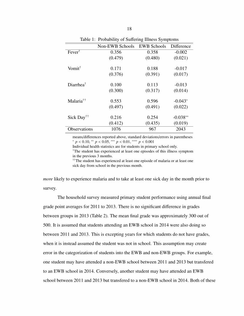
18
Table 1: Probability of Suffering Illness SymptomsNon-EWB Schools EWB Schools Difference
Fever† 0.356 0.358 -0.002(0.479) (0.480) (0.021)
Vomit† 0.171 0.188 -0.017(0.376) (0.391) (0.017)
Diarrhea† 0.100 0.113 -0.013(0.300) (0.317) (0.014)
Malaria†† 0.553 0.596 -0.043∗
(0.497) (0.491) (0.022)
Sick Day†† 0.216 0.254 -0.038∗∗
(0.412) (0.435) (0.019)Observations 1076 967 2043
means/differences reported above, standard deviations/errors in parentheses∗ p < 0.10, ∗∗ p < 0.05, ∗∗∗ p < 0.01, ∗∗∗∗ p < 0.001Individual health statistics are for students in primary school only.†The student has experienced at least one episodes of this illness symptomin the previous 3 months.††The student has experienced at least one episode of malaria or at least onesick day from school in the previous month.
more likely to experience malaria and to take at least one sick day in the month prior to
survey.
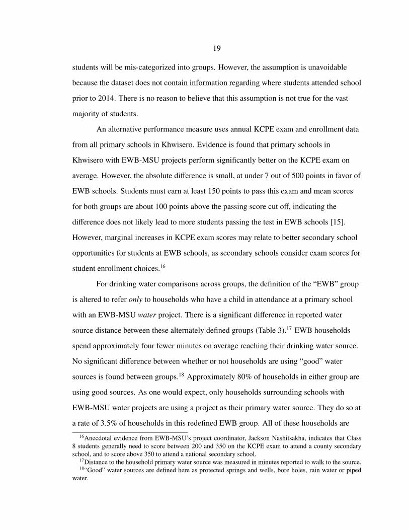
The household survey measured primary student performance using annual final
grade point averages for 2011 to 2013. There is no significant difference in grades
between groups in 2013 (Table 2). The mean final grade was approximately 300 out of
500. It is assumed that students attending an EWB school in 2014 were also doing so
between 2011 and 2013. This is excepting years for which students do not have grades,
when it is instead assumed the student was not in school. This assumption may create
error in the categorization of students into the EWB and non-EWB groups. For example,
one student may have attended a non-EWB school between 2011 and 2013 but transfered
to an EWB school in 2014. Conversely, another student may have attended an EWB
school between 2011 and 2013 but transfered to a non-EWB school in 2014. Both of these
19
students will be mis-categorized into groups. However, the assumption is unavoidable
because the dataset does not contain information regarding where students attended school
prior to 2014. There is no reason to believe that this assumption is not true for the vast
majority of students.
An alternative performance measure uses annual KCPE exam and enrollment data
from all primary schools in Khwisero. Evidence is found that primary schools in
Khwisero with EWB-MSU projects perform significantly better on the KCPE exam on
average. However, the absolute difference is small, at under 7 out of 500 points in favor of
EWB schools. Students must earn at least 150 points to pass this exam and mean scores
for both groups are about 100 points above the passing score cut off, indicating the
difference does not likely lead to more students passing the test in EWB schools [15].
However, marginal increases in KCPE exam scores may relate to better secondary school
opportunities for students at EWB schools, as secondary schools consider exam scores for
student enrollment choices.16
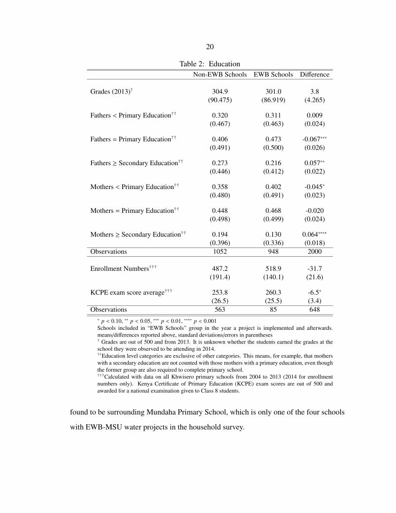
For drinking water comparisons across groups, the definition of the “EWB” group
is altered to refer only to households who have a child in attendance at a primary school
with an EWB-MSU water project. There is a significant difference in reported water
source distance between these alternately defined groups (Table 3).17 EWB households
spend approximately four fewer minutes on average reaching their drinking water source.
No significant difference between whether or not households are using “good” water
sources is found between groups.18 Approximately 80% of households in either group are
using good sources. As one would expect, only households surrounding schools with
EWB-MSU water projects are using a project as their primary water source. They do so at
a rate of 3.5% of households in this redefined EWB group. All of these households are
16Anecdotal evidence from EWB-MSU’s project coordinator, Jackson Nashitsakha, indicates that Class8 students generally need to score between 200 and 350 on the KCPE exam to attend a county secondaryschool, and to score above 350 to attend a national secondary school.
17Distance to the household primary water source was measured in minutes reported to walk to the source.18“Good” water sources are defined here as protected springs and wells, bore holes, rain water or piped
water.
20
Table 2: EducationNon-EWB Schools EWB Schools Difference
Grades (2013)† 304.9 301.0 3.8(90.475) (86.919) (4.265)
Fathers < Primary Education†† 0.320 0.311 0.009(0.467) (0.463) (0.024)
Fathers = Primary Education†† 0.406 0.473 -0.067∗∗∗
(0.491) (0.500) (0.026)
Fathers ≥ Secondary Education†† 0.273 0.216 0.057∗∗
(0.446) (0.412) (0.022)
Mothers < Primary Education†† 0.358 0.402 -0.045∗
(0.480) (0.491) (0.023)
Mothers = Primary Education†† 0.448 0.468 -0.020(0.498) (0.499) (0.024)
Mothers ≥ Secondary Education†† 0.194 0.130 0.064∗∗∗∗
(0.396) (0.336) (0.018)Observations 1052 948 2000
Enrollment Numbers††† 487.2 518.9 -31.7(191.4) (140.1) (21.6)
KCPE exam score average††† 253.8 260.3 -6.5∗
(26.5) (25.5) (3.4)Observations 563 85 648∗ p < 0.10, ∗∗ p < 0.05, ∗∗∗ p < 0.01, ∗∗∗∗ p < 0.001Schools included in “EWB Schools” group in the year a project is implemented and afterwards.means/differences reported above, standard deviations/errors in parentheses† Grades are out of 500 and from 2013. It is unknown whether the students earned the grades at theschool they were observed to be attending in 2014.††Education level categories are exclusive of other categories. This means, for example, that motherswith a secondary education are not counted with those mothers with a primary education, even thoughthe former group are also required to complete primary school.†††Calculated with data on all Khwisero primary schools from 2004 to 2013 (2014 for enrollmentnumbers only). Kenya Certificate of Primary Education (KCPE) exam scores are out of 500 andawarded for a national examination given to Class 8 students.
found to be surrounding Mundaha Primary School, which is only one of the four schools
with EWB-MSU water projects in the household survey.
21
Table 3: Drinking WaterWet Season Dry Season
Household Group Non-EWB EWB Diff. Non-EWB EWB Diff.
Dist. to Primary Water Source (min.) 16.0 12.2 3.8∗∗∗ 17.0 12.9 4.1∗∗∗∗
(15.5) (12.6) (1.2) (13.8) (11.9) (1.1)
Treat Water † 0.583 0.678 -0.095∗∗ 0.583 0.678 -0.095∗∗
(0.493) (0.468) (0.040) (0.493) (0.468) (0.040)
Treat Water in House†† 0.403 0.467 -0.065 0.403 0.467 -0.065(0.491) (0.500) (0.041) (0.491) (0.500) (0.041)
Good Water Source††† 0.834 0.869 -0.035 0.768 0.799 -0.031(0.372) (0.338) (0.030) (0.423) (0.402) (0.034)
Spring (protected) 0.418 0.347 0.072∗ 0.503 0.447 0.056(0.494) (0.477) (0.040) (0.500) (0.498) (0.041)
Spring (unprotected) 0.043 0.030 0.013 0.064 0.035 0.029(0.204) (0.171) (0.016) (0.245) (0.185) (0.019)
Rain 0.217 0.246 -0.029 0.002 0.010 -0.008(0.413) (0.432) (0.034) (0.042) (0.100) (0.005)
Public Tap 0.099 0.090 0.009 0.156 0.136 0.021(0.299) (0.288) (0.024) (0.363) (0.343) (0.029)
Household Pipe 0.023 0.090 -0.068∗∗∗∗ 0.026 0.095 -0.069∗∗∗∗
(0.149) (0.288) (0.016) (0.159) (0.295) (0.017)
River/Stream 0.106 0.090 0.015 0.148 0.151 -0.003(0.308) (0.288) (0.025) (0.355) (0.359) (0.029)
Well (protected) 0.064 0.045 0.019 0.068 0.055 0.012(0.245) (0.208) (0.019) (0.251) (0.229) (0.020)
Well (unprotected) 0.012 0.010 0.002 0.017 0.015 0.002(0.110) (0.100) (0.009) (0.131) (0.122) (0.011)
Bore Hole Well 0.012 0.015 -0.003 0.012 0.020 -0.008(0.110) (0.122) (0.009) (0.110) (0.141) (0.010)
EWB Bore Hole 0.000 0.035 -0.035∗∗∗∗ 0.000 0.035 -0.035∗∗∗∗
(0.000) (0.185) (0.008) (0.000) (0.185) (0.008)
Lake/Pond 0.003 0.000 0.003 0.002 0.000 0.002(0.059) (0.000) (0.004) (0.042) (0.000) (0.003)
Observations 576 199 775 576 199 775∗ p < 0.10, ∗∗ p < 0.05, ∗∗∗ p < 0.01, ∗∗∗∗ p < 0.001The EWB group is restricted here to households surrounding EWB schools with water projects, only. This is done to specifi-cally examine the relationship between EWB-MSU water projects and household water use. Means/differences reported above,standard deviations/errors in parentheses†indicates the household always treats drinking water in house or the drinking water is treated at the source.††indicates the household always treats drinking water in house.†††“Good” indicates the source is piped, a protected ground source (including bore hole wells) or rain water and excludes anysurface or unprotected source.
22
Other Variables of Interest
The following summarized outcomes are not expected to be impacted by
EWB-MSU projects but are likely related to the outcomes of interest: health, education
and time-use. As mentioned above, evaluating differences between groups in these
dimensions provides evidence regarding whether the non-EWB group is an approximate
counterfactual for the EWB group.
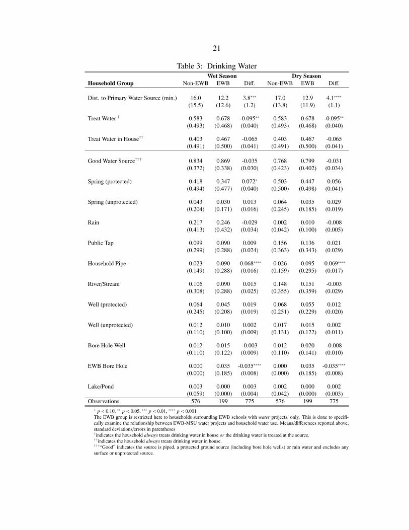
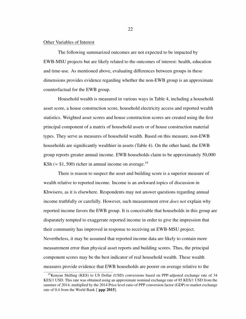
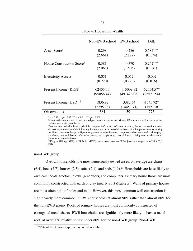
Household wealth is measured in various ways in Table 4, including a household
asset score, a house construction score, household electricity access and reported wealth
statistics. Weighted asset scores and house construction scores are created using the first
principal component of a matrix of household assets or of house construction material
types. They serve as measures of household wealth. Based on this measure, non-EWB
households are significantly wealthier in assets (Table 4). On the other hand, the EWB
group reports greater annual income. EWB households claim to be approximately 50,000
KSh (≈ $1, 500) richer in annual income on average.19
There is reason to suspect the asset and building score is a superior measure of
wealth relative to reported income. Income is an awkward topics of discussion in
Khwisero, as it is elsewhere. Respondents may not answer questions regarding annual
income truthfully or carefully. However, such measurement error does not explain why
reported income favors the EWB group. It is conceivable that households in this group are
disparately tempted to exaggerate reported income in order to give the impression that
their community has improved in response to receiving an EWB-MSU project.
Nevertheless, it may be assumed that reported income data are likely to contain more
measurement error than physical asset reports and building scores. Thus, the principal
component scores may be the best indicator of real household wealth. These wealth
measures provide evidence that EWB households are poorer on average relative to the19Kenyan Shilling (KES) to US Dollar (USD) conversions based on PPP-adjusted exchange rate of 34
KES/1 USD. This rate was obtained using an approximate nominal exchange rate of 85 KES/1 USD from thesummer of 2014, multiplied by the 2014 Price level ratio of PPP conversion factor (GDP) to market exchangerate of 0.4 from the World Bank [˙ppp˙2015].
23
Table 4: Household Wealth
Non-EWB school EWB school Diff.
Asset Score† 0.298 -0.286 0.584∗∗∗∗
(2.661) (2.127) (0.174)
House Construction Score† 0.381 -0.370 0.752∗∗∗∗
(2.068) (1.505) (0.131)
Electricity Access 0.051 0.052 -0.002(0.220) (0.223) (0.016)
Present Income (KES)†† 62455.35 115009.92 -52554.57∗∗
(95056.44) (491426.08) (25571.54)
Present Income (USD)†† 1836.92 3382.64 -1545.72∗∗
(2795.78) (14453.71) (752.10)Observations 384 391 775
∗ p < 0.10, ∗∗ p < 0.05, ∗∗∗ p < 0.01, ∗∗∗∗ p < 0.001Income and assets are self reported and subject to measurement error. Means/differences reported above, standarddeviations/errors in parentheses†Scores calculated with the first principle component of a matrix of assets or primary house construction materi-als. Assets are numbers of the following: houses, carts, hoes, motorbikes, boats, bicycles, plows, tractors, sewingmachines, lanterns or lamps, refrigerators, generators, wheelbarrows, computers, radios, water tanks, video play-ers, chairs, cars, cellphones, sofas, solar panels, beds, cupboards, chest of drawers, dining sets, watches, drums(instrument) and televisions.††Kenyan Shilling (KES) to US Dollar (USD) conversions based on PPP-adjusted exchange rate of 34 KES/1USD.
non-EWB group.
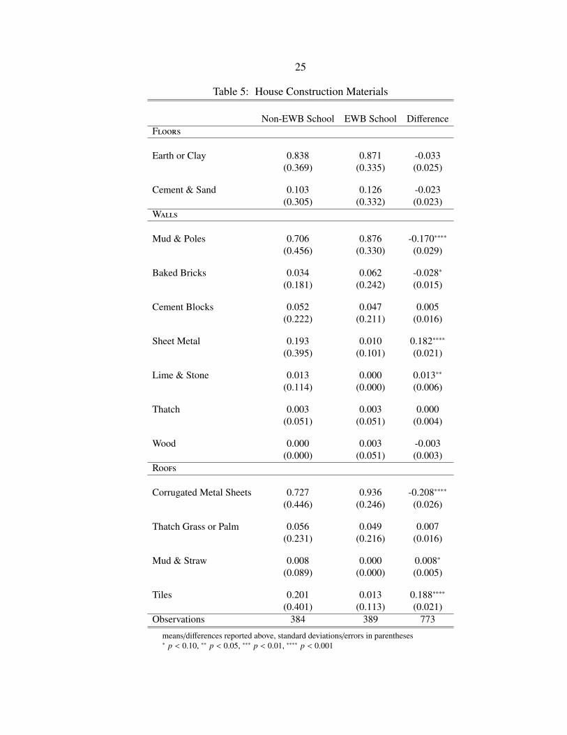
Over all households, the most numerously owned assets on average are chairs
(6.4), hoes (2.7), houses (2.3), sofas (2.1), and beds (1.9).20 Households are least likely to
own cars, boats, tractors, plows, generators, and computers. Primary house floors are most
commonly constructed with earth or clay (nearly 90%)(Table 5). Walls of primary houses
are most often built of poles and mud. However, this most common wall construction is
significantly more common in EWB households at almost 90% rather than almost 80% for
the non-EWB group. Roofs of primary houses are most commonly constructed of
corrugated metal sheets. EWB households are significantly more likely to have a metal
roof, at over 90% relative to just under 80% for the non-EWB group. Non-EWB
20Rate of asset ownership is not reported in a table.
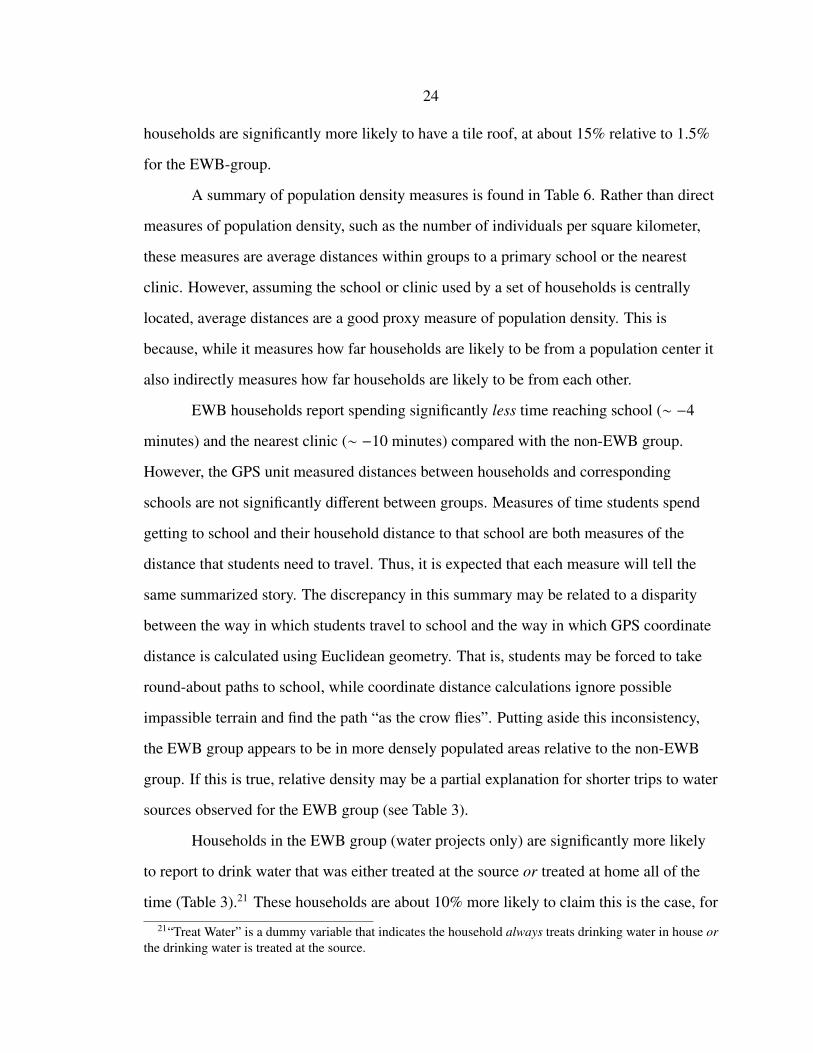
24
households are significantly more likely to have a tile roof, at about 15% relative to 1.5%
for the EWB-group.
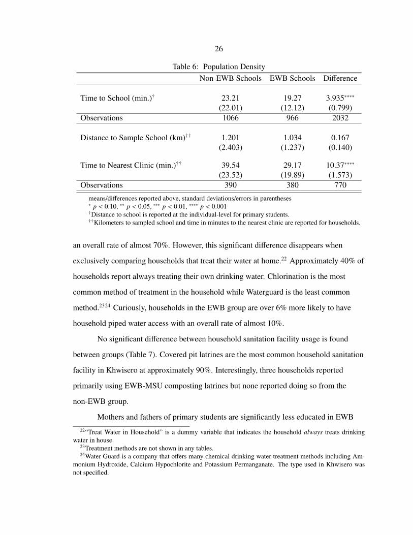
A summary of population density measures is found in Table 6. Rather than direct
measures of population density, such as the number of individuals per square kilometer,
these measures are average distances within groups to a primary school or the nearest
clinic. However, assuming the school or clinic used by a set of households is centrally
located, average distances are a good proxy measure of population density. This is
because, while it measures how far households are likely to be from a population center it
also indirectly measures how far households are likely to be from each other.
EWB households report spending significantly less time reaching school (∼ −4
minutes) and the nearest clinic (∼ −10 minutes) compared with the non-EWB group.
However, the GPS unit measured distances between households and corresponding
schools are not significantly different between groups. Measures of time students spend
getting to school and their household distance to that school are both measures of the
distance that students need to travel. Thus, it is expected that each measure will tell the
same summarized story. The discrepancy in this summary may be related to a disparity
between the way in which students travel to school and the way in which GPS coordinate
distance is calculated using Euclidean geometry. That is, students may be forced to take
round-about paths to school, while coordinate distance calculations ignore possible
impassible terrain and find the path “as the crow flies”. Putting aside this inconsistency,
the EWB group appears to be in more densely populated areas relative to the non-EWB
group. If this is true, relative density may be a partial explanation for shorter trips to water
sources observed for the EWB group (see Table 3).
Households in the EWB group (water projects only) are significantly more likely
to report to drink water that was either treated at the source or treated at home all of the
time (Table 3).21 These households are about 10% more likely to claim this is the case, for
21“Treat Water” is a dummy variable that indicates the household always treats drinking water in house orthe drinking water is treated at the source.
25
Table 5: House Construction Materials
Non-EWB School EWB School DifferenceFloors
Earth or Clay 0.838 0.871 -0.033(0.369) (0.335) (0.025)
Cement & Sand 0.103 0.126 -0.023(0.305) (0.332) (0.023)
Walls
Mud & Poles 0.706 0.876 -0.170∗∗∗∗
(0.456) (0.330) (0.029)
Baked Bricks 0.034 0.062 -0.028∗
(0.181) (0.242) (0.015)
Cement Blocks 0.052 0.047 0.005(0.222) (0.211) (0.016)
Sheet Metal 0.193 0.010 0.182∗∗∗∗
(0.395) (0.101) (0.021)
Lime & Stone 0.013 0.000 0.013∗∗
(0.114) (0.000) (0.006)
Thatch 0.003 0.003 0.000(0.051) (0.051) (0.004)
Wood 0.000 0.003 -0.003(0.000) (0.051) (0.003)
Roofs
Corrugated Metal Sheets 0.727 0.936 -0.208∗∗∗∗
(0.446) (0.246) (0.026)
Thatch Grass or Palm 0.056 0.049 0.007(0.231) (0.216) (0.016)
Mud & Straw 0.008 0.000 0.008∗
(0.089) (0.000) (0.005)
Tiles 0.201 0.013 0.188∗∗∗∗
(0.401) (0.113) (0.021)Observations 384 389 773
means/differences reported above, standard deviations/errors in parentheses∗ p < 0.10, ∗∗ p < 0.05, ∗∗∗ p < 0.01, ∗∗∗∗ p < 0.001
26
Table 6: Population DensityNon-EWB Schools EWB Schools Difference
Time to School (min.)† 23.21 19.27 3.935∗∗∗∗
(22.01) (12.12) (0.799)Observations 1066 966 2032
Distance to Sample School (km)†† 1.201 1.034 0.167(2.403) (1.237) (0.140)
Time to Nearest Clinic (min.)†† 39.54 29.17 10.37∗∗∗∗
(23.52) (19.89) (1.573)Observations 390 380 770
means/differences reported above, standard deviations/errors in parentheses∗ p < 0.10, ∗∗ p < 0.05, ∗∗∗ p < 0.01, ∗∗∗∗ p < 0.001†Distance to school is reported at the individual-level for primary students.††Kilometers to sampled school and time in minutes to the nearest clinic are reported for households.
an overall rate of almost 70%. However, this significant difference disappears when
exclusively comparing households that treat their water at home.22 Approximately 40% of
households report always treating their own drinking water. Chlorination is the most
common method of treatment in the household while Waterguard is the least common
method.2324 Curiously, households in the EWB group are over 6% more likely to have
household piped water access with an overall rate of almost 10%.
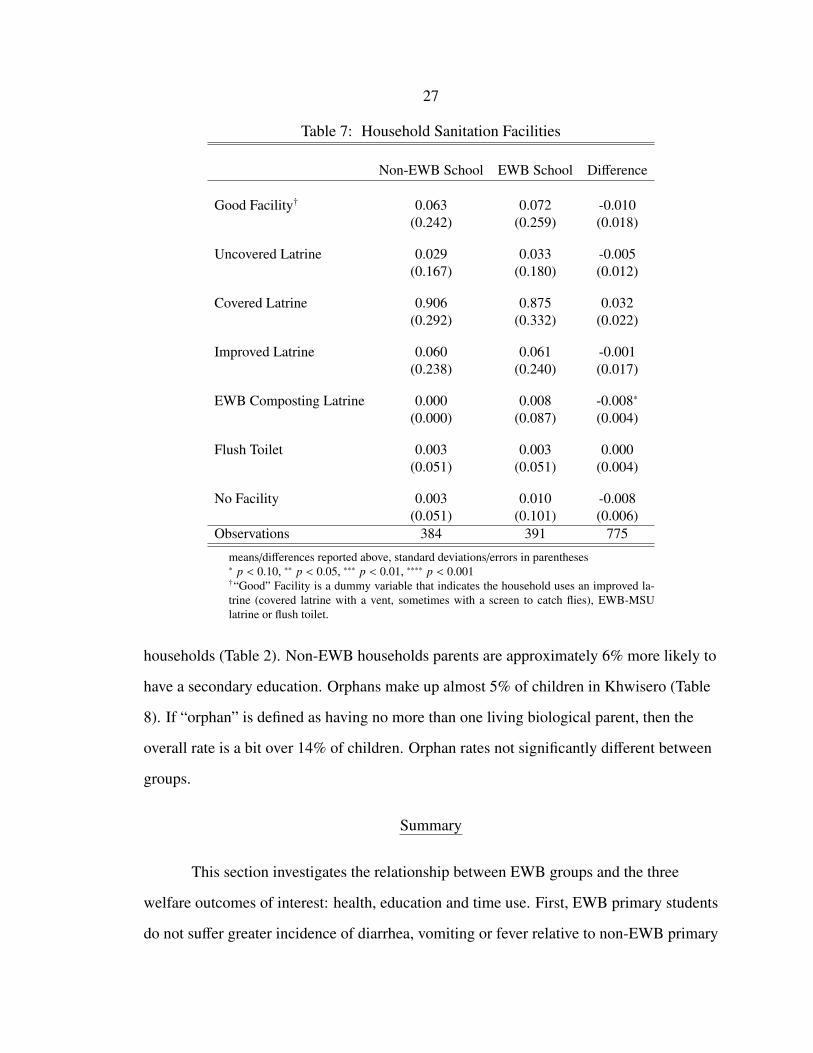
No significant difference between household sanitation facility usage is found
between groups (Table 7). Covered pit latrines are the most common household sanitation
facility in Khwisero at approximately 90%. Interestingly, three households reported
primarily using EWB-MSU composting latrines but none reported doing so from the
non-EWB group.
Mothers and fathers of primary students are significantly less educated in EWB
22“Treat Water in Household” is a dummy variable that indicates the household always treats drinkingwater in house.
23Treatment methods are not shown in any tables.24Water Guard is a company that offers many chemical drinking water treatment methods including Am-
monium Hydroxide, Calcium Hypochlorite and Potassium Permanganate. The type used in Khwisero wasnot specified.
27
Table 7: Household Sanitation Facilities
Non-EWB School EWB School Difference
Good Facility† 0.063 0.072 -0.010(0.242) (0.259) (0.018)
Uncovered Latrine 0.029 0.033 -0.005(0.167) (0.180) (0.012)
Covered Latrine 0.906 0.875 0.032(0.292) (0.332) (0.022)
Improved Latrine 0.060 0.061 -0.001(0.238) (0.240) (0.017)
EWB Composting Latrine 0.000 0.008 -0.008∗
(0.000) (0.087) (0.004)
Flush Toilet 0.003 0.003 0.000(0.051) (0.051) (0.004)
No Facility 0.003 0.010 -0.008(0.051) (0.101) (0.006)
Observations 384 391 775
means/differences reported above, standard deviations/errors in parentheses∗ p < 0.10, ∗∗ p < 0.05, ∗∗∗ p < 0.01, ∗∗∗∗ p < 0.001†“Good” Facility is a dummy variable that indicates the household uses an improved la-trine (covered latrine with a vent, sometimes with a screen to catch flies), EWB-MSUlatrine or flush toilet.
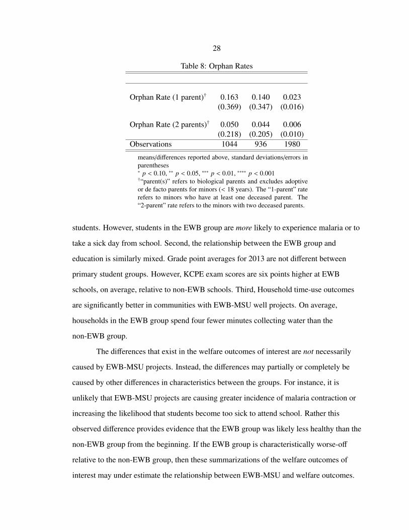
households (Table 2). Non-EWB households parents are approximately 6% more likely to
have a secondary education. Orphans make up almost 5% of children in Khwisero (Table
8). If “orphan” is defined as having no more than one living biological parent, then the
overall rate is a bit over 14% of children. Orphan rates not significantly different between
groups.
Summary
This section investigates the relationship between EWB groups and the three
welfare outcomes of interest: health, education and time use. First, EWB primary students
do not suffer greater incidence of diarrhea, vomiting or fever relative to non-EWB primary
28
Table 8: Orphan Rates
Orphan Rate (1 parent)† 0.163 0.140 0.023(0.369) (0.347) (0.016)
Orphan Rate (2 parents)† 0.050 0.044 0.006(0.218) (0.205) (0.010)
Observations 1044 936 1980
means/differences reported above, standard deviations/errors inparentheses∗ p < 0.10, ∗∗ p < 0.05, ∗∗∗ p < 0.01, ∗∗∗∗ p < 0.001†“parent(s)” refers to biological parents and excludes adoptiveor de facto parents for minors (< 18 years). The “1-parent” raterefers to minors who have at least one deceased parent. The“2-parent” rate refers to the minors with two deceased parents.
students. However, students in the EWB group are more likely to experience malaria or to
take a sick day from school. Second, the relationship between the EWB group and
education is similarly mixed. Grade point averages for 2013 are not different between
primary student groups. However, KCPE exam scores are six points higher at EWB
schools, on average, relative to non-EWB schools. Third, Household time-use outcomes
are significantly better in communities with EWB-MSU well projects. On average,
households in the EWB group spend four fewer minutes collecting water than the
non-EWB group.
The differences that exist in the welfare outcomes of interest are not necessarily
caused by EWB-MSU projects. Instead, the differences may partially or completely be
caused by other differences in characteristics between the groups. For instance, it is
unlikely that EWB-MSU projects are causing greater incidence of malaria contraction or
increasing the likelihood that students become too sick to attend school. Rather this
observed difference provides evidence that the EWB group was likely less healthy than the
non-EWB group from the beginning. If the EWB group is characteristically worse-off
relative to the non-EWB group, then these summarizations of the welfare outcomes of
interest may under estimate the relationship between EWB-MSU and welfare outcomes.
29
Thus, the true impacts of the projects are likely entangled with other factors.
This section also investigates the relationship between the EWB group and other
outcomes not expected to be impacted by EWB-MSU. Although the EWB and non-EWB
groups are similar to one another regarding some characteristics, they differ in other
notable characteristics. Each group is generally equivalent in primary household
construction materials, sanitation facilities and orphan rates. However, households in the
non-EWB group appear wealthier and to have better educated parents. Households in the
EWB group appear to be located in more densely populated areas and have significantly
greater access to piped water in household compounds. This final descriptive difference in
piped water access suggests that EWB-MSU’s relationship with shorter water trips is
partially explained by a higher rate of piped water access within the EWB group.
The descriptive evidence does suggest that EWB-MSU is successfully prioritizing
less well-off schools for project construction. It also suggests that the non-EWB group is
not a good approximation of the EWB group’s counterfactual. That is, had an EWB-MSU
project not been constructed, EWB primary school students and their households might
have already experienced worse outcomes in health, education and time-use relative to the
non-EWB group. This conclusion illustrates the importance of utilizing empirical
methods that control for selection bias. These are detailed in the following section.
30
EMPIRICAL METHODOLOGY
To test the welfare impact of Engineers Without Borders’ water and sanitation
projects, schools that have received projects are to be compared with schools that have not
in order to examine the differences in welfare outcomes. However, EWB-MSU’s projects
are not randomized control trials, nor is the project treatment restricted to a single set of
individuals, for the EWB and non-EWB groups may change over time. These facts give
rise to two identification concerns.
First, as shown in the previous section, EWB communities are characteristically
distinct from non-EWB communities. On the one hand, the non-EWB group appears to be
wealthier and have better educated parents. These differences likely lead to worse welfare
outcomes that conflict with the potential positive impact of EWB-MSU projects. Thus,
these characteristics may understate the organization’s relationship with welfare. On the
other hand, EWB communities appear more densely populated and to have greater access
to piped water.25 These characteristic differences may overstate the organization’s impact
by positively affecting welfare outcomes simultaneously with EWB-MSU projects.
Second, an additional threat to identification is the possibility that households with
certain characteristics may be more likely to send their children to an EWB school in
order to have access to a project. Of these characteristics, only some may be observed,
such as wealth and parental education. However, other characteristics may not be
observed in these data. Positive welfare outcomes related to EWB-MSU may partially be
explained by these households changing the characteristic composition of the EWB group
over time. This may overstate the relationship between EWB-MSU projects and welfare
outcomes, as projects are expected to simultaneously improve welfare outcomes.
Anecdotal evidence from EWB-MSU’s project coordinator, Jackson Nashitsakha,
25When using the aggregated school data, characteristic differences may be even greater, as the 21 schoolswith EWB-MSU projects are compared with more than 40 other primary schools around Khwisero. This isbecause many of these other schools are not being considered for future projects, as are schools in the surveycategorized in the non-EWB group. Thus, these schools presumably experience even better welfare outcomesthan both EWB schools and non-EWB schools.
31
suggests student’s do not transfer to EWB schools in response to project implementation.
However, the possibility of such individual-level endogeneity will motivate the use of
empirical methods to safe-guard against it.
In order to identify EWB-MSU’s impact on welfare outcomes, the two forms of
selection bias presented here need to be controlled. The following is an elaboration of the
empirical methodology designed to do so. In the subsequent results section, these
strategies are used to estimate the impact of EWB-MSU projects on welfare outcomes.
Method (1): Ordinary Least Squares
Let all individual or household characteristics that determines EWB-MSU project
placement, as well as one’s attendance at an EWB school, be known and observed. If
these characteristics are held constant, then any remaining variation in attendance at an
EWB school, EWBi, is random and the variable is said to be conditionally independent of
the outcome of interest, yi. Ordinary least squares analysis relies on the conditional
independence assumption (CIA) in order to interpret the coefficient, δ, as the causal effect
of EWBi on yi. This method is mathematically represented in Equation (1). The EWBi
dummy variable indicates either that primary student i is attending an EWB school or that
household i was selected from an EWB school parent list. All relevant characteristics that
allow the CIA are contained in the conditioning set xi. If the CIA holds, then selection
bias at the community or household-level is controlled because any information that leads
to this bias is held constant in the xi set.
yi = α + δEWBi + xi · β + εi (1)
In practice, the estimate of EWB-MSU’s impact, δ, may be biased if relevant
characteristics for the CIA are omitted from xi. Let the set xi for each i be stacked into
matrix X, and let there exist another unobserved or unknown set of individual and
32
household characteristics, W, such that the correlation between X and W is non-zero and
the correlation between W and yi is non-zero. In this case, omitted variable bias exists in
the estimate δ because it identifies variation in both EWBi and W that affects yi.
The conditioning matrix, X, varies by model. For household-level models,
characteristics measured in X include a household asset score, house construction score,
the head’s education-level, the household’s water and sanitation source quality and
whether the household treats its water. For individual-level models, the control variable
matrix includes those previously mentioned with the addition of age, gender, orphan status
and parental education-level and excluding household head’s education level. Each of
these control variables is included because they are expected to explain variation in
welfare outcomes, and many are additionally related to EWB-MSU project placement and
EWB school attendance.
Method (2): Fixed Effect
In addition to the observed control variables, there may exist other unobserved
characteristics that relate to EWB-MSU project placement, EWB school attendance and
welfare outcomes. For example, Typhoid virus may be common in a community that
EWB-MSU selects for project placement. The prevalence of the virus in that community
will independently affect health outcomes. However, given that Typhoid is unobserved as
well as related to EWB-MSU project placement, its omission from a model explaining
health outcomes will bias the estimated impact of the organization.
The set of characteristics held by individual i has a fixed effect on the outcome of
interest yi,t across time, t.26 That is, i’s characteristics, be they observed or otherwise, have
an average effect on yi,t that is constant in time. These individual fixed effects may also
correlate with EWB-MSU project placement or EWB school attendance. Without
controlling for i’s fixed effect, ρi, some unobserved portion of this variation may be
26For convenience, the discussion prototype for Method (2) will be an individual-level model. However,in practice, Method (2) will be applied to individual, household and school-level data.
33
inappropriately captured in δ, the effect of EWB-MSU on yi,t. However, including
individual fixed effects in the regression will remove selection bias in the estimate of δ that
is caused by these time-invariant characteristics. This fixed effect estimation strategy is
represented mathematically in Equation (2).
yi,t = α + δEWBi,t + τt + ρi + εi,t (2)
Time-series data are required in order to observe i’s fixed effect on the outcome of
interest across time. However, there may additionally be an effect of each year t on yi,t that
is constant across individuals. For instance, increasing wealth over time is expected to
improve welfare outcomes for both EWB and non-EWB students in Khwisero. Including
a time fixed effect, τt, removes variation in the outcome of interest explained by any such
factors that are constant across individuals in year t.
In Equation 2, the variable EWBi,t is a treatment dummy indicating i has access to
an EWB-MSU project. In the individual-level models, EWBi,t indicates individual i is
attending a primary school that received an EWB-MSU project in year t or prior. In the
household-level models, EWBi,t indicates that household i was selected from a school that
has received an EWB-MSU project in year t or prior. In the school-level models, EWBi,t
indicates that school i has received an EWB-MSU project in year t or prior.
The coefficient δ is the average effect of access to an EWB-MSU project on
outcome yi,t. If yi,t measures a desirable outcome, such as average grade points, then the
estimate of EWB-MSU impact, δ, is expected to be positive. Accordingly, if the outcome
of interest measures undesirable outcomes, then the estimated effect is expected to be
negative. Time is expected to relate positively to welfare outcomes because of wealth
growth.27 The magnitude and sign of each individual fixed effect estimate, ρi will depend
on the ith individual’s time-invariant characteristics.27Kenya has experience between 4-9% annual GDP growth between 2010 to 2013 [˙world˙2015].
34
EWB and non-EWB group specific time trends in the outcomes of interest are a
further identification concern for estimating EWB-MSU’s impact with individual fixed
effects. Neither the estimated individual fixed effects or year fixed effects control for
variation in yi,t explained by disparate time trends, because the former is constant across t
and the later is constant across i. If these trends are identical, δ is an estimate of the
variation in yi,t explained exclusively by EWB-MSU projects. However, if the trends are
not identical across time, the difference will be picked up in the estimated effect of
EWB-MSU because of the trends dependence on the EWBi,t dummy. Hence, δ will be
biased.
The dataset used in this analysis provides limited time-series data for use with the
fixed effect methodology. The analysis will utilize retrospective measures of welfare
outcomes and school-level time-series data. Unfortunately, other covariates related to the
outcomes of interest, yi,t, do not exist in this dataset prior to the Summer of 2014. Thus,
any other covariates otherwise used as control variables may not be used in Method (2).
Some of these covariates may measure time-variant characteristics that are related to yi,t.
Such variation over time may be the cause of unequal time trends between the EWB and
non-EWB group, leading to a biased estimate of δ. However, if it is assumed that all
characteristics relevant to explaining welfare outcomes have a time-invariant effect on
welfare outcomes, then the set’s covariation with yi,t is completely captured by the
coefficient, ρi.
Method (3): Instrumental Variables
As previously indicated, there may remain other characteristics of EWB schools
and households with children who attend those schools that are not observed in the
dataset. These unobserved characteristics may be correlated with welfare outcomes as
well as the likelihood of receiving an EWB-MSU project or the likelihood of sending
children to primary schools with EWB-MSU projects. Another approach utilizes distance
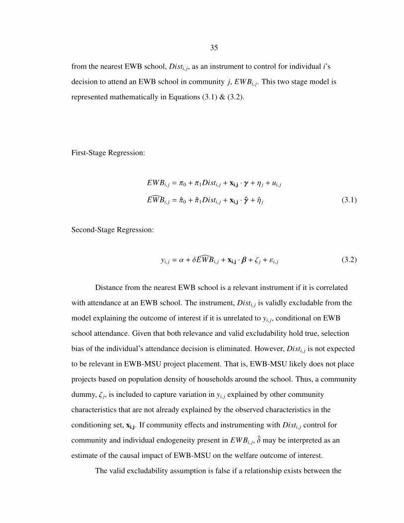
35
from the nearest EWB school, Disti, j, as an instrument to control for individual i’s
decision to attend an EWB school in community j, EWBi, j. This two stage model is
represented mathematically in Equations (3.1) & (3.2).
First-Stage Regression:
EWBi, j = π0 + π1Disti, j + xi,j · γ + η j + ui, j
EWBi, j = π0 + π1Disti, j + xi,j · γ + η j (3.1)
Second-Stage Regression:
yi, j = α + δEWBi, j + xi,j · β + ζ j + εi, j (3.2)
Distance from the nearest EWB school is a relevant instrument if it is correlated
with attendance at an EWB school. The instrument, Disti, j is validly excludable from the
model explaining the outcome of interest if it is unrelated to yi, j, conditional on EWB
school attendance. Given that both relevance and valid excludability hold true, selection
bias of the individual’s attendance decision is eliminated. However, Disti, j is not expected
to be relevant in EWB-MSU project placement. That is, EWB-MSU likely does not place
projects based on population density of households around the school. Thus, a community
dummy, ζ j, is included to capture variation in yi, j explained by other community
characteristics that are not already explained by the observed characteristics in the
conditioning set, xi,j. If community effects and instrumenting with Disti, j control for
community and individual endogeneity present in EWBi, j, δ may be interpreted as an
estimate of the causal impact of EWB-MSU on the welfare outcome of interest.
The valid excludability assumption is false if a relationship exists between the
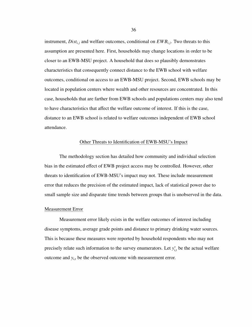
36
instrument, Disti, j and welfare outcomes, conditional on EWBi, j. Two threats to this
assumption are presented here. First, households may change locations in order to be
closer to an EWB-MSU project. A household that does so plausibly demonstrates
characteristics that consequently connect distance to the EWB school with welfare
outcomes, conditional on access to an EWB-MSU project. Second, EWB schools may be
located in population centers where wealth and other resources are concentrated. In this
case, households that are farther from EWB schools and populations centers may also tend
to have characteristics that affect the welfare outcome of interest. If this is the case,
distance to an EWB school is related to welfare outcomes independent of EWB school
attendance.
Other Threats to Identification of EWB-MSU’s Impact
The methodology section has detailed how community and individual selection
bias in the estimated effect of EWB project access may be controlled. However, other
threats to identification of EWB-MSU’s impact may not. These include measurement
error that reduces the precision of the estimated impact, lack of statistical power due to
small sample size and disparate time trends between groups that is unobserved in the data.
Measurement Error
Measurement error likely exists in the welfare outcomes of interest including
disease symptoms, average grade points and distance to primary drinking water sources.
This is because these measures were reported by household respondents who may not
precisely relate such information to the survey enumerators. Let y∗i,t be the actual welfare
outcome and yi,t be the observed outcome with measurement error.
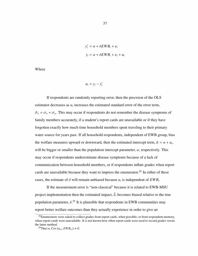
37
y∗i = α + δEWBi + εi
yi = α + δEWBi + εi + ui
Where
ui = yi − y∗i
If respondents are randomly reporting error, then the precision of the OLS
estimator decreases as ui increases the estimated standard error of the error term,
σε = σε + σu. This may occur if respondents do not remember the disease symptoms of
family members accurately, if a student’s report cards are unavailable or if they have
forgotten exactly how much time household members spent traveling to their primary
water source for years past. If all household respondents, independent of EWB group, bias
the welfare measures upward or downward, then the estimated intercept term, α = α + ui,
will be bigger or smaller than the population intercept parameter, α, respectively. This
may occur if respondents underestimate disease symptoms because of a lack of
communication between household members, or if respondents inflate grades when report
cards are unavailable because they want to impress the enumerator.28 In either of these
cases, the estimate of δ will remain unbiased because ui is independent of EWBi.
If the measurement error is “non-classical” because it is related to EWB-MSU
project implementation then the estimated impact, δ, becomes biased relative to the true
population parameter, δ.29 It is plausible that respondents in EWB communities may
report better welfare outcomes than they actually experience in order to give an
28Enumerators were asked to collect grades from report cards, when possible; or from respondent memory,when report cards were unavailable. It is not known how often report cards were used to record grades versusthe latter method.
29That is, Cov(ui,t, EWBi,t
), 0.
38
impression that EWB-MSU projects are working. In this case, the estimate δ will be
biased upwards. Alternatively, respondents may report worse outcomes than truly
experienced in hopes of receiving another project. In this case, δ will instead be biased
downward.30 Ultimately, whether these data contain biased measurement error is
unknowable. The potential implications of measurement error in the outcome measures is
considered throughout the subsequent empirical results.
Measurement error is unlikely to be an issue in the explanatory variable of interest,
EWBi. Instead, it seems likely that household respondents will know which members are
attending which schools and if those schools have an EWB-MSU project. Further, there is
no reason to suspect respondents might claim a household member is not a student at an
EWB school when they truly are, and vice versa. However, measurement error may exist
in i’s reported distance to the nearest EWB school, Disti. This variable is used as an
instrument for attendance at an EWB school. Respondents from the EWB group may
report distance to EWB schools with greater accuracy than non-EWB group households
leading to variance of the error term that is related to the explanatory variable of interest.
This heteroskedasticity of the error term will lead generally to over-estimated standard
errors for EWB-group households and increase the likelihood of a false negative test.
Whites heteroskedasticity-consistent standard errors are used in these models as a
safe-guard to this potential issue.
Statistical Power & Group-Specific Time Trends
Lacking statistical power and group specific time trends are further threats to
identification of EWB-MSU’s impact. Even if EWB-MSU has an impact on welfare
outcomes, the likelihood of detecting such impact may be low due to the sample size.
Further, the effect of group specific time trends is not addressed with the methodology.
Such disparate trends may correlate with group designation while simultaneously affecting
30The the bias will make estimate δ inconsistent. Mathematically, for all γ > 0 and n observations sampledfrom this population, as n → ∞ the functional estimate δ(n) does not consistently estimate the populationparameter δ. That is, limn→∞ P
[|δ(n) − δ∗| > γ
], 0
39
the rate of change in welfare outcomes. Thus, without controlling for the potential
differences in time trends, the estimated impact of EWB-MSU projects may be biased.
40
RESULTS
The structure of the data that measure the three outcomes of interest determines
which Methods, (1), (2) or (3), from the previous section are used to test EWB-MSU’s
impact. First, EWB-MSU’s relationship with several health outcomes is estimated with
ordinary least squares (OLS) and instrumental variables, Methods (1) & (3). These
methods are selected because health measures were collected for a single point in time
and, thus, only non-panel data OLS and instrumental variables are appropriate. Health
estimates are provided in Table 9. Second, the impact of EWB school attendance on
student average grade points is estimated with OLS and individual fixed effects, Methods
(1) & (2). Fixed effect methods are selected, in addition to OLS, because education
outcomes were collected for multiple points in time. These estimates are provided in
Table 14. Further, EWB-MSU’s impact on education is tested using school fixed effects
and school-level measures of KCPE exam performance and enrollment numbers. These
estimates are presented in Table 15. Third, the effect of EWB-MSU’s water projects on
household time spent collecting water is estimated with OLS and household fixed effects,
Methods (1) & (2). Fixed effect methods are also appropriate for this analysis because
time-use measures were collected for multiple points in time. These estimates may be
found in Table 12.
EWB-MSU’s Impact on Health
EWB-MSU’s impact on primary student health outcomes is tested using OLS and
instrumental variables, Methods (1) & (3). Contrary to expectations, estimates do not
provide evidence that EWB-MSU is positively impacting health outcomes. In fact,
evidence to support a relationship between reported health outcomes and any covariates in
the data are difficult to find in these models. Further, R2 values are exceptionally low in
these models. This may partially be explained by measurement error in health outcomes.
This error may lead to insignificant relationships with many covariates due to higher
41
standard errors. Alternatively, this may be explained by omitted control variables that
explain variation in health outcomes.31
Ordinary Least Squares Estimates
Estimates for the impact of EWB-MSU on probability of experiencing illness
symptoms using Method (1) are presented in Table 9.32 Health outcomes are generally
unrelated to whether or not a student attends an EWB school. The exception to this is
observed in the OLS estimates for malaria morbidity. However, contrary to expectation
attending an EWB school has a positive relationship with the probability of contracting
malaria in the previous year by about 9%.
In this model, the control variable matrix includes age, gender, household asset
score and house construction score, parental education level, distance to the nearest clinic,
and dummies for “good” household water source, water treatment in house, and “good”
household sanitation source. Further, community fixed effects are included that capture
other unobserved characteristics that may related to EWB-MSU project placement.
Contrary to expectations, none of these controls are consistently found to relate
significantly with health outcomes with the exception of age. Age relates negatively with
diarrhea, vomiting and malaria, as expected.
Unexpectedly, good water source and the asset score are significantly and
positively related to one of the disease symptoms. Both are signals of wealth, which
should related to decreases in illness. Further, having a good water source should help
household members avoid enteric disease. Nevertheless, conditional on control variables,
students are almost 2% more likely to experience vomiting in the previous three months
per relative point in their household’s asset score. Further, students from households with
31The notably small R2 values in the instrumental variables models is further explained by unique calcu-lation of the value for this estimation strategy. In instrumental variables, the total sum of squares (TSS) isallowed to be larger than the sum of squared residuals (RSS), in contrast to estimates in ordinary least squares.
32 Table 18 in Appendix B also contains OLS and instrumental variables estimates for the relationshipbetween EWB-MSU projects and health. However, the dependent variable in Table 18 is instead the numberof illness episodes experienced by the individual student in the past three months. The results are effectivelyequivalent in regards to EWB-MSU’s impact on health.
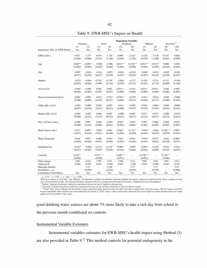
42
Table 9: EWB-MSU’s Impact on Health
Dependent Variable:Diarrhea Fever Vomitting Malaria† Sick Day††
(1) (2) (3) (4) (5) (6) (7) (8) (9) (10)Instrument: Dist. to EWB School No Yes No Yes No Yes No Yes No Yes
EWB (indiv.) 0.021 1.275 0.034 1.150 0.096∗ 2.523∗∗ 0.116 -1.728 0.119∗ -0.861(0.046) (0.800) (0.073) (1.100) (0.058) (1.258) (0.075) (1.268) (0.065) (0.989)
Age -0.007∗∗∗ -0.008∗∗ -0.006 -0.006 -0.015∗∗∗∗ -0.018∗∗∗∗ -0.016∗∗∗∗ -0.013∗∗ 0.000 0.000(0.002) (0.003) (0.004) (0.005) (0.003) (0.005) (0.004) (0.005) (0.004) (0.004)
Girl -0.007 -0.016 -0.014 -0.035 -0.002 -0.018 -0.009 -0.015 -0.025 -0.026(0.017) (0.022) (0.027) (0.030) (0.021) (0.035) (0.027) (0.035) (0.024) (0.027)
Orphan -0.025 -0.064 -0.218∗∗ -0.239∗∗ -0.084 -0.177 0.105 0.214 -0.151∗ -0.108(0.062) (0.084) (0.098) (0.116) (0.078) (0.133) (0.101) (0.134) (0.088) (0.104)
Asset Score -0.002 -0.005 0.001 0.003 0.014∗∗∗ 0.010 0.014∗∗ 0.018∗∗ 0.006 0.009(0.004) (0.005) (0.007) (0.007) (0.005) (0.008) (0.007) (0.009) (0.006) (0.007)
House Construction Score 0.002 0.005 -0.013 -0.012 -0.026∗∗∗ -0.019 -0.013 -0.021 -0.002 -0.006(0.006) (0.008) (0.010) (0.011) (0.008) (0.013) (0.010) (0.013) (0.009) (0.010)
Father Edu. Level -0.003 0.008 0.004 0.007 -0.011 -0.001 0.010 0.008 -0.005 -0.008(0.007) (0.010) (0.011) (0.013) (0.009) (0.015) (0.012) (0.016) (0.010) (0.012)
Mother Edu. Level -0.001 -0.001 0.004 0.007 -0.000 0.005 0.017 0.013 -0.009 -0.010(0.008) (0.011) (0.013) (0.015) (0.011) (0.017) (0.014) (0.017) (0.012) (0.014)
Dist. to Clinic (min.) 0.000 0.001 -0.001 -0.001 -0.001∗∗ -0.001 0.001 0.000 -0.001 -0.001(0.000) (0.001) (0.001) (0.001) (0.001) (0.001) (0.001) (0.001) (0.001) (0.001)
Water Source (dry) 0.011 0.059∗ -0.003 0.064 0.064∗∗ 0.132∗∗ -0.005 -0.044 0.106∗∗∗∗ 0.085∗
(0.021) (0.036) (0.033) (0.049) (0.026) (0.056) (0.034) (0.056) (0.029) (0.044)
Water Treatment 0.018 0.031 0.046 0.029 0.011 0.029 -0.043 -0.077∗ -0.041 -0.068∗∗
(0.020) (0.026) (0.031) (0.036) (0.025) (0.042) (0.032) (0.042) (0.028) (0.033)
Sanitation Fac. -0.033 -0.040 -0.114∗∗ -0.118∗∗ -0.082∗∗ -0.087 -0.099∗ -0.120∗ 0.016 0.014(0.033) (0.042) (0.052) (0.058) (0.042) (0.066) (0.054) (0.066) (0.047) (0.052)
Constant 0.182∗∗∗ – 0.547∗∗∗∗ – 0.460∗∗∗∗ – 0.736∗∗∗∗ – 0.328∗∗∗∗ –(0.056) (0.090) (0.071) (0.092) (0.080)
Observations 1292 1212 1292 1212 1292 1212 1292 1212 1292 1212Adjusted R2 -0.001 -0.657 0.016 -0.204 0.047 -1.398 0.032 -0.500 0.030 -0.187Hausman Statistic – 4.17 – 11.09 – 2.77 – 3.71 – 3.33Probability > χ2
12 – (0.965) – (0.436) – (0.993) – (0.978) – (0.986)Community Fixed Effects Yes Yes Yes Yes Yes Yes Yes Yes Yes Yes∗ p < 0.10, ∗∗ p < 0.05, ∗∗∗ p < 0.01, ∗∗∗∗ p < 0.001With the exception of “Sick Day” and ”Malaria”, the dependent variables are dummies indicating whether the primary student has experienced the illness symptom at leastonce in the past three months. All school fixed effects estimated in lieu of a constant term but none are not shown. Standard errors are in parentheses.†“Malaria” indicates the primary student has experienced at least one case of malaria in the past year.††“Sick Day” indicates the primary student has experienced at least one day off from school due to illness in the past month.†††“Good” Water Source indicates the household is using a protected spring, protected well, bore hole, rain water or piped water in the dry season. The dry season is specifiedbecause households often switch to rain water during the wet season; a “good” source. Using a good source during the dry season might be a better measure of the year roundquality of the household’s water source.
good drinking water sources are about 7% more likely to take a sick day from school in
the previous month conditional on controls.
Instrumental Variable Estimates
Instrumental variables estimates for EWB-MSU’s health impact using Method (3)
are also provided in Table 9.32 This method controls for potential endogeneity in the
43
choice to attend an EWB school, and community fixed effects capture other community
characteristics that may cause selection bias in project implementation. There remains
almost no detectable impact on health outcomes contrary to expectations. The
goodness-of-fit statistics are very low, indicating low explanation of variation in health
outcomes.
EWB school attendance is instrumented with distance to the nearest EWB school.
The first stage regression is reported in Table 10. There are three apparent problems with
this instrument. First, the instrument forms a weak relationship with the variable of
interest, EWBi, j. The F-test for joint significance reports a F-statistic just below the
threshold for a non-weak instrument.33 Further, the R2 value is low in the first-stage,
indicating the right-hand-side variables poorly explain variation in EWB school
attendance. Each of these statistics indicate that EWBi, j is weakly identified. Second, the
distance instrument may not be validly excluded from a model explaining health
outcomes. Table 11 provides some evidence that distance to the nearest EWB school is
positively related to the mother’s education level.34 Further, distance to the student’s
primary school (i.e. not necessarily an EWB school) is positively related to wealth
measures. In turn, wealth and parental education levels are related to the child’s health
outcomes. This constitutes evidence that distance is not exogenous to models explaining
health and, therefore, an invalid instrument for EWB school attendance. Finally, the
Hausman statistics fail to reject the null hypothesis that EWBi, j is exogenous to the error
term, εi, j. Assuming that the IV estimator is consistently estimating EWB-MSU’s impact
on health, these statistics provide some evidence that individual endogeneity in school
attendance does not exist. That is, student’s are not transferring to EWB schools in order
to gain access to a project. This backs up anecdotal evidence provided by EWB-MSU’s
33An F-statistic for joint significance is generally regarded to identify a weak instrument when below 10.The statistic reported in Table 10 is approximately 9.5.
34Evidence is also found that distance to school is negatively related to the father’s education level. It isunclear why the relationship between distance and paternal education would be inverse to the correspondingrelationship with maternal education.
44
project coordinator, Jackson Nashitsakha.
The uncertainty regarding relevance and valid excludability of distance as an
instrument for EWBi, j may indicate there exists bias in the estimates for EWB-MSU’s
impact on health. If the instrument exogeneity condition does not hold then the estimate
bias worsens with a weaker relationship between the instrument and the explanatory
variables.35 Bias in the instrumental variable estimator may partially explain the lack of
significance in instrumented estimates for the impact of EWB-MSU health outcomes.
Further, Hausman statistics indicate instrumentation for individual-level endogeneity may
be unnecessary in the first place.
EWB-MSU Impact on Time-Use
EWB-MSU’s impact on time-use is tested with ordinary least squares and fixed
effects Methods (1) & (2). Each empirical strategy is applied to two models, one for the
wet season and one for the dry. The division is made in order to remove variation
explained by changing water sources during the wet season, relative to the dry.36 For these
time-use models, the right-hand-side variable of interest, EWBi,t, indicates a water project
has been implemented at a school, at which household i has a student in attendance in year
t, excepting OLS models where t = 2014. This removes from the “treatment” group
households that send students to EWB schools with latrines, which are not expected to
receive any time-use benefits in water collection.
Ordinary Least Squares Estimates
Households selected from parent lists at EWB schools with bore hole well projects
spend less time collecting water during the dry season, conditional on wealth and water
source type (Table 12). These households spend a little over two and a quarter fewer
35To see this mathematically, first construct the instrumental variables estimator with matrix notation,βIV = (Z′X)−1Z′y, where Z is the explanatory variable matrix from the first stage regression. AssumingE [Z′ε] , 0, the expected value of the estimator, E
[βIV
]= β + E
[(Z′X)−1Z′ε
], becomes increasingly biased
as Cov (Z′X)→ 0.36For a discussion of this variation, see the Outcomes subsection in the Data Description section.
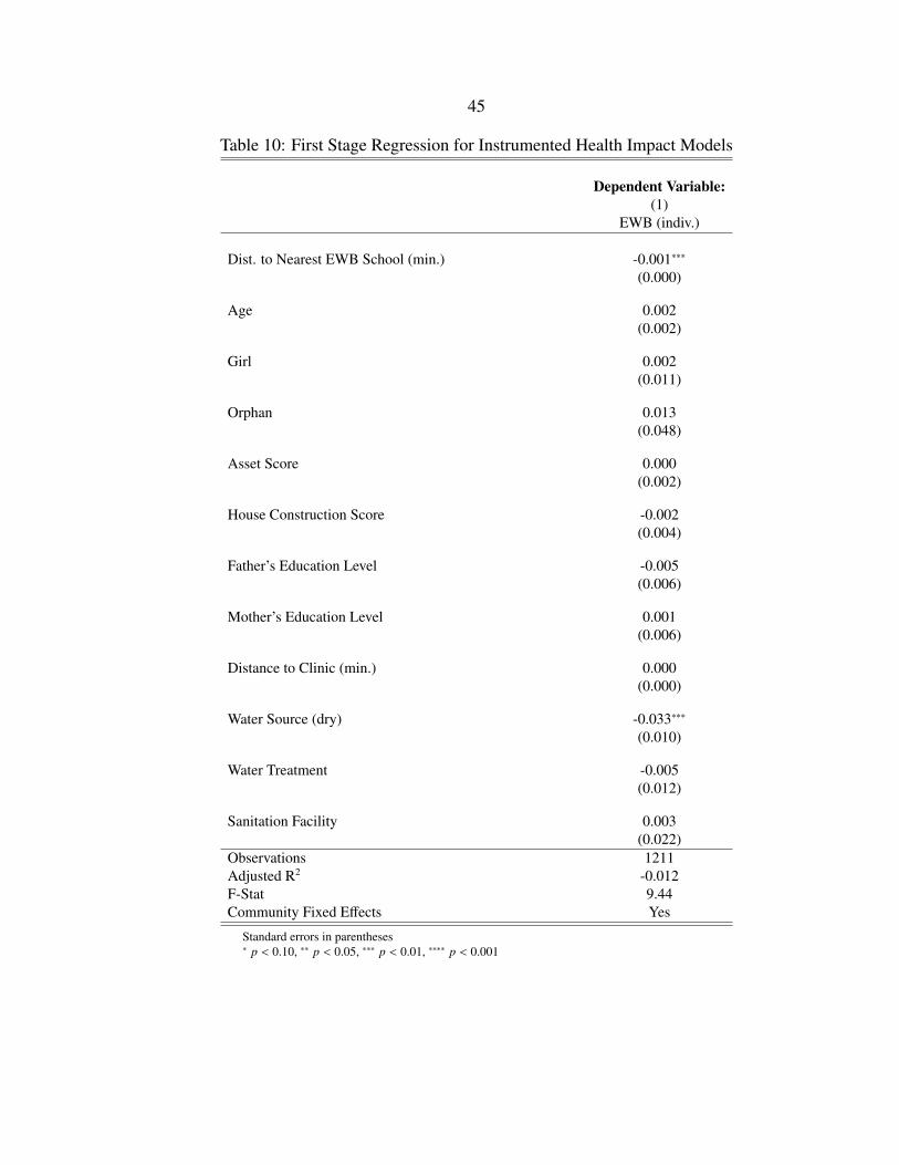
45
Table 10: First Stage Regression for Instrumented Health Impact Models
Dependent Variable:(1)
EWB (indiv.)
Dist. to Nearest EWB School (min.) -0.001∗∗∗
(0.000)
Age 0.002(0.002)
Girl 0.002(0.011)
Orphan 0.013(0.048)
Asset Score 0.000(0.002)
House Construction Score -0.002(0.004)
Father’s Education Level -0.005(0.006)
Mother’s Education Level 0.001(0.006)
Distance to Clinic (min.) 0.000(0.000)
Water Source (dry) -0.033∗∗∗
(0.010)
Water Treatment -0.005(0.012)
Sanitation Facility 0.003(0.022)
Observations 1211Adjusted R2 -0.012F-Stat 9.44Community Fixed Effects Yes
Standard errors in parentheses∗ p < 0.10, ∗∗ p < 0.05, ∗∗∗ p < 0.01, ∗∗∗∗ p < 0.001
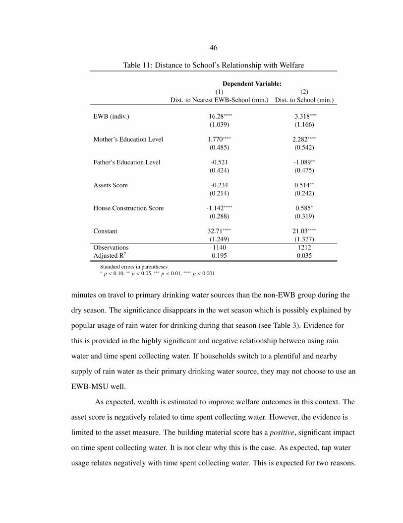
46
Table 11: Distance to School’s Relationship with Welfare
Dependent Variable:(1) (2)
Dist. to Nearest EWB-School (min.) Dist. to School (min.)
EWB (indiv.) -16.28∗∗∗∗ -3.318∗∗∗
(1.039) (1.166)
Mother’s Education Level 1.770∗∗∗∗ 2.282∗∗∗∗
(0.485) (0.542)
Father’s Education Level -0.521 -1.089∗∗
(0.424) (0.475)
Assets Score -0.234 0.514∗∗
(0.214) (0.242)
House Construction Score -1.142∗∗∗∗ 0.585∗
(0.288) (0.319)
Constant 32.71∗∗∗∗ 21.03∗∗∗∗
(1.249) (1.377)Observations 1140 1212Adjusted R2 0.195 0.035
Standard errors in parentheses∗ p < 0.10, ∗∗ p < 0.05, ∗∗∗ p < 0.01, ∗∗∗∗ p < 0.001
minutes on travel to primary drinking water sources than the non-EWB group during the
dry season. The significance disappears in the wet season which is possibly explained by
popular usage of rain water for drinking during that season (see Table 3). Evidence for
this is provided in the highly significant and negative relationship between using rain
water and time spent collecting water. If households switch to a plentiful and nearby
supply of rain water as their primary drinking water source, they may not choose to use an
EWB-MSU well.
As expected, wealth is estimated to improve welfare outcomes in this context. The
asset score is negatively related to time spent collecting water. However, the evidence is
limited to the asset measure. The building material score has a positive, significant impact
on time spent collecting water. It is not clear why this is the case. As expected, tap water
usage relates negatively with time spent collecting water. This is expected for two reasons.
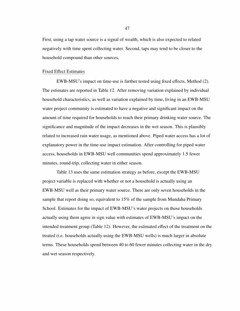
47
First, using a tap water source is a signal of wealth, which is also expected to related
negatively with time spent collecting water. Second, taps may tend to be closer to the
household compound than other sources.
Fixed Effect Estimates
EWB-MSU’s impact on time-use is further tested using fixed effects, Method (2).
The estimates are reported in Table 12. After removing variation explained by individual
household characteristics, as well as variation explained by time, living in an EWB-MSU
water project community is estimated to have a negative and significant impact on the
amount of time required for households to reach their primary drinking water source. The
significance and magnitude of the impact decreases in the wet season. This is plausibly
related to increased rain water usage, as mentioned above. Piped water access has a lot of
explanatory power in the time-use impact estimation. After controlling for piped water
access, households in EWB-MSU well communities spend approximately 1.5 fewer
minutes, round-trip, collecting water in either season.
Table 13 uses the same estimation strategy as before, except the EWB-MSU
project variable is replaced with whether or not a household is actually using an
EWB-MSU well as their primary water source. There are only seven households in the
sample that report doing so, equivalent to 15% of the sample from Mundaha Primary
School. Estimates for the impact of EWB-MSU’s water projects on those households
actually using them agree in sign value with estimates of EWB-MSU’s impact on the
intended treatment group (Table 12). However, the estimated effect of the treatment on the
treated (i.e. households actually using the EWB-MSU wells) is much larger in absolute
terms. These households spend between 40 to 60 fewer minutes collecting water in the dry
and wet season respectively.
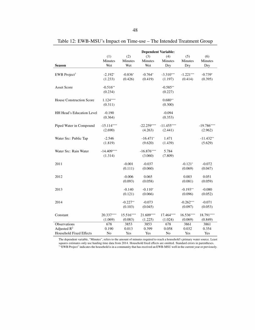
48
Table 12: EWB-MSU’s Impact on Time-use – The Intended Treatment Group
Dependent Variable:(1) (2) (3) (4) (5) (6)
Minutes Minutes Minutes Minutes Minutes MinutesSeason Wet Wet Wet Dry Dry Dry
EWB Project† -2.192∗ -0.836∗ -0.764∗ -3.310∗∗∗ -1.221∗∗∗ -0.739∗
(1.233) (0.426) (0.419) (1.197) (0.414) (0.395)
Asset Score -0.516∗∗ -0.585∗∗
(0.234) (0.227)
House Construction Score 1.124∗∗∗∗ 0.680∗∗
(0.311) (0.300)
HH Head’s Education Level -0.190 -0.094(0.364) (0.353)
Piped Water in Compound -15.114∗∗∗∗ -22.259∗∗∗∗ -11.455∗∗∗∗ -19.786∗∗∗∗
(2.690) (4.263) (2.441) (2.962)
Water Src: Public Tap -2.546 -16.471∗ 1.471 -11.432∗∗
(1.819) (9.620) (1.439) (5.629)
Water Src: Rain Water -14.409∗∗∗∗ -16.876∗∗∗∗ 5.784(1.314) (3.060) (7.809)
2011 -0.001 -0.037 -0.121∗ -0.072(0.111) (0.060) (0.069) (0.047)
2012 -0.006 0.065 0.003 0.051(0.093) (0.058) (0.081) (0.059)
2013 -0.140 -0.110∗ -0.193∗∗ -0.080(0.121) (0.066) (0.096) (0.052)
2014 -0.227∗∗ -0.073 -0.262∗∗∗ -0.071(0.103) (0.045) (0.097) (0.053)
Constant 20.337∗∗∗∗ 15.516∗∗∗∗ 21.609∗∗∗∗ 17.464∗∗∗∗ 16.536∗∗∗∗ 18.791∗∗∗∗
(1.069) (0.083) (1.225) (1.024) (0.069) (0.849)Observations 678 3853 3853 678 3861 3861Adjusted R2 0.190 0.013 0.399 0.058 0.032 0.354Household Fixed Effects No Yes Yes No Yes Yes
The dependent variable, “Minutes”, refers to the amount of minutes required to reach a household’s primary water source. Leastsquares estimates only use hauling time data from 2014. Household fixed effects are omitted. Standard errors in parentheses.†“EWB Project” indicates the household is in a community that has received an EWB-MSU well in the current year or previously.
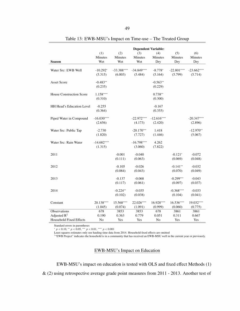
49
Table 13: EWB-MSU’s Impact on Time-use – The Treated Group
Dependent Variable:(1) (2) (3) (4) (5) (6)
Minutes Minutes Minutes Minutes Minutes MinutesSeason Wet Wet Wet Dry Dry Dry
Water Src: EWB Well -10.292∗ -33.388∗∗∗∗ -34.849∗∗∗∗ -8.778∗ -22.801∗∗∗∗ -23.662∗∗∗∗
(5.315) (6.003) (5.484) (5.164) (5.799) (5.714)
Asset Score -0.483∗∗ -0.563∗∗
(0.235) (0.229)
House Construction Score 1.158∗∗∗∗ 0.738∗∗
(0.310) (0.300)
HH Head’s Education Level -0.255 -0.167(0.364) (0.355)
Piped Water in Compound -16.030∗∗∗∗ -22.972∗∗∗∗ -12.616∗∗∗∗ -20.347∗∗∗∗
(2.656) (4.173) (2.420) (2.896)
Water Src: Public Tap -2.730 -20.170∗∗∗ 1.418 -12.970∗∗
(1.820) (7.727) (1.446) (5.067)
Water Src: Rain Water -14.682∗∗∗∗ -16.798∗∗∗∗ 4.262(1.315) (3.060) (7.822)
2011 -0.001 -0.040 -0.121∗ -0.072(0.111) (0.063) (0.069) (0.048)
2012 -0.105 -0.026 -0.141∗∗ -0.032(0.084) (0.043) (0.070) (0.049)
2013 -0.137 -0.068 -0.299∗∗∗ -0.043(0.117) (0.061) (0.097) (0.037)
2014 -0.224∗∗ -0.035 -0.368∗∗∗∗ -0.033(0.102) (0.038) (0.104) (0.041)
Constant 20.138∗∗∗∗ 15.568∗∗∗∗ 22.026∗∗∗∗ 16.928∗∗∗∗ 16.536∗∗∗∗ 19.032∗∗∗∗
(1.045) (0.074) (1.091) (0.999) (0.060) (0.775)Observations 678 3853 3853 678 3861 3861Adjusted R2 0.190 0.363 0.779 0.051 0.311 0.667Household Fixed Effects No Yes Yes No Yes Yes
Standard errors in parentheses∗ p < 0.10, ∗∗ p < 0.05, ∗∗∗ p < 0.01, ∗∗∗∗ p < 0.001Least squares estimates only use hauling time data from 2014. Household fixed effects are omitted†“EWB Project” indicates the household is in a community that has received an EWB-MSU well in the current year or previously.
EWB-MSU’s Impact on Education
EWB-MSU’s impact on education is tested with OLS and fixed effect Methods (1)
& (2) using retrospective average grade point measures from 2011 - 2013. Another test of
50
EWB-MSU’s impact on education uses Method (2) on enrollment and KCPE exam scores
from all Khwisero primary schools. No evidence is found for an impact on education
outcomes.
There are at least two explanations for the lack of observed impact on education.
First, this analysis hasn’t found evidence of an EWB-MSU impact on health outcomes.
Additionally, time-use impacts are limited to a small number of households. Thus, If
EWB-MSU is not meaningfully affecting health and time-use outcomes, and these are the
only two vectors through which education improvements are expected, then an
EWB-MSU impact on education outcomes clearly cannot be expected. Second, Khwisero
primary schools likely use relative grading schemes. If grading is entirely relative then a
welfare shock that uniformly affects all students is not expected to change the relative
grades for any specific student. Thus, even if EWB-MSU projects improve the educational
performance of all students at a school equally, relative grades will obscure the effect.
However, this explanation does not apply to the lack of observed impact on KCPE exam
scores and enrollment, each measured relative to other schools.
Ordinary Least Squares Estimates
Whether or not an individual attends an EWB school does not have a significant
relationship with 2013 student grade point averages according to Method (1) estimates
(Table 14). Other covariates are estimated to form an expected relationship with education
outcomes. Whether or not a household always treats water at home is significantly and
positively related to grade point by a large absolute margin. Students from these
households score an average of about 17 points higher on a 500 point scale, than do those
students from households that do not treat. A possible explanation of this may be the
characteristics of households that treat water at home also positively influence the
household pupils’ academic performance. Alternatively, the pupil’s health benefits from
treated water translate into academic benefits at school. The relationship between water
treatment and grade points provides some evidence that improved health is indeed a vector
51
for improved education outcomes.
Of the wealth measures, only household construction quality appears to relate
significantly to grade point outcomes. The father’s education level is also significantly and
positively related. For every increment in level of education of the father, the student’s
grade point gains almost 5 points.37 It appears that fathers who are well educated are also
likely to have high achieving sons and daughters. Curiously, the same relationship does
not exist between mothers and offspring in these data.
Contrary to expectation, age is negatively related to grade point outcomes. The
student’s gender is not significantly related to grade point. Further, covariates, including
clinic distance, “good” household drinking water source and sanitation facility, are not
estimated to have a significant relationship with education outcomes as expected.
Fixed Effect Estimates
The fixed effect Method (2) is used to test EWB-MSU’s impact on primary student
grade point outcomes. These estimates are also reported in Table 14.38 After removing
variation explained by individual fixed effects and time fixed effects, the impact of
attending a school with an EWB-MSU project on grade points remains unknown. As
mentioned above, it is perhaps unsurprising that an EWB-MSU project, which presumably
benefits all students at the school equally, doesn’t affect grade points within a relativistic
grading regime.
A positive and significant effect of 2013 (the 3rd year) is detected on grades across
primary schools. It is unclear what occurred that year that would lead to an overall
increase in grade points. The relationship of time and grade points provides some
evidence that grades are at least partially absolute rather than purely relativistic. That is,
teachers may compare students to fixed achievement goals rather than exclusively to each
37The education level of the parent of minor (< 18 years) i is measured by partial or full completionof standard institutional academic levels. That is, (0) “none”, (1) “some primary school”, (2) “completedprimary school”, (3) “some secondary”, and so on.
38The individual fixed effects are not reported.
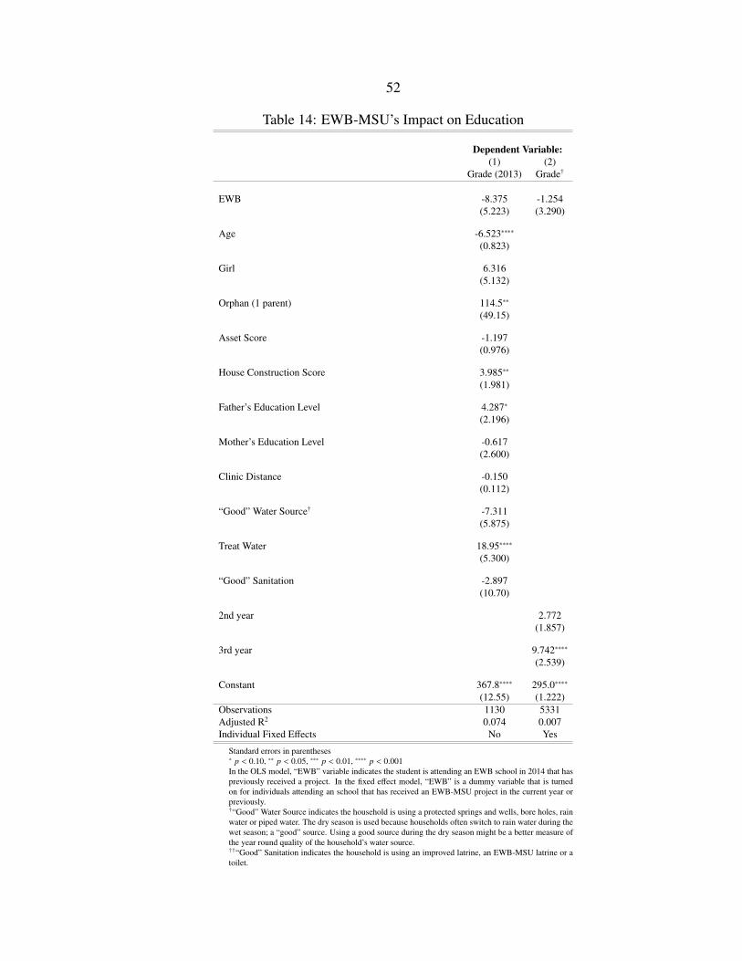
52
Table 14: EWB-MSU’s Impact on Education
Dependent Variable:(1) (2)
Grade (2013) Grade†
EWB -8.375 -1.254(5.223) (3.290)
Age -6.523∗∗∗∗
(0.823)
Girl 6.316(5.132)
Orphan (1 parent) 114.5∗∗
(49.15)
Asset Score -1.197(0.976)
House Construction Score 3.985∗∗
(1.981)
Father’s Education Level 4.287∗
(2.196)
Mother’s Education Level -0.617(2.600)
Clinic Distance -0.150(0.112)
“Good” Water Source† -7.311(5.875)
Treat Water 18.95∗∗∗∗
(5.300)
“Good” Sanitation -2.897(10.70)
2nd year 2.772(1.857)
3rd year 9.742∗∗∗∗
(2.539)
Constant 367.8∗∗∗∗ 295.0∗∗∗∗
(12.55) (1.222)Observations 1130 5331Adjusted R2 0.074 0.007Individual Fixed Effects No Yes
Standard errors in parentheses∗ p < 0.10, ∗∗ p < 0.05, ∗∗∗ p < 0.01, ∗∗∗∗ p < 0.001In the OLS model, “EWB” variable indicates the student is attending an EWB school in 2014 that haspreviously received a project. In the fixed effect model, “EWB” is a dummy variable that is turnedon for individuals attending an school that has received an EWB-MSU project in the current year orpreviously.†“Good” Water Source indicates the household is using a protected springs and wells, bore holes, rainwater or piped water. The dry season is used because households often switch to rain water during thewet season; a “good” source. Using a good source during the dry season might be a better measure ofthe year round quality of the household’s water source.††“Good” Sanitation indicates the household is using an improved latrine, an EWB-MSU latrine or atoilet.
53
other. Otherwise, overall average grade points would not change over time.
Method (2) is also used to test EWB-MSU’s impact on education outcomes at the
school-level. These estimates relate to enrollment and average test score on the KCPE
exam as the outcome of interest. After controlling for school fixed-effects and year fixed
effects, there is no evidence that EWB-MSU is impacting education outcomes at the
school-level either. This confirms the findings from the individual-level models and is
similarly unsurprising due to the lack of evidence for an EWB-MSU health impact.
Estimates of the effect of years 2012 and 2013 provide some evidence that Khwisero
primary students in Class 8 are performing better than the area average on KCPE exams in
recent years. It is also clear from year estimates that enrollment in Khwisero primary
schools is growing over time.
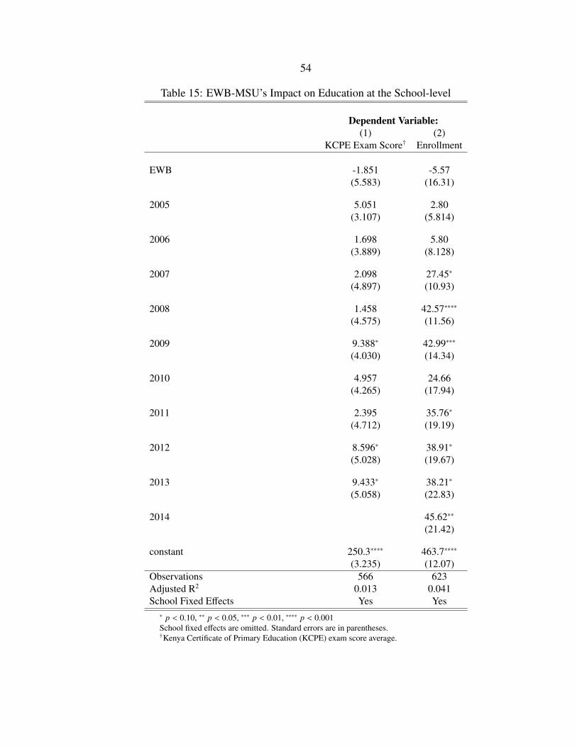
54
Table 15: EWB-MSU’s Impact on Education at the School-level
Dependent Variable:(1) (2)
KCPE Exam Score† Enrollment
EWB -1.851 -5.57(5.583) (16.31)
2005 5.051 2.80(3.107) (5.814)
2006 1.698 5.80(3.889) (8.128)
2007 2.098 27.45∗
(4.897) (10.93)
2008 1.458 42.57∗∗∗∗
(4.575) (11.56)
2009 9.388∗ 42.99∗∗∗
(4.030) (14.34)
2010 4.957 24.66(4.265) (17.94)
2011 2.395 35.76∗
(4.712) (19.19)
2012 8.596∗ 38.91∗
(5.028) (19.67)
2013 9.433∗ 38.21∗
(5.058) (22.83)
2014 45.62∗∗
(21.42)
constant 250.3∗∗∗∗ 463.7∗∗∗∗
(3.235) (12.07)Observations 566 623Adjusted R2 0.013 0.041School Fixed Effects Yes Yes∗ p < 0.10, ∗∗ p < 0.05, ∗∗∗ p < 0.01, ∗∗∗∗ p < 0.001School fixed effects are omitted. Standard errors are in parentheses.†Kenya Certificate of Primary Education (KCPE) exam score average.
55
CONCLUSION
Estimation of the effect EWB-MSU has on welfare outcomes in Khwisero, Kenya
was the primary goal of this research. The analysis does not provide evidence that
EWB-MSU water and sanitation projects affect health or education outcomes. However, it
does find evidence that EWB-MSU water projects reduce the amount of time households
spend collecting water. On average, households in communities with EWB-MSU water
projects are spending approximately 1.5 fewer minutes per trip collecting drinking water.
Only 7 households in the sample, or approximately 4% of sampled households
surrounding EWB-MSU water projects, are using the projects as their primary water
source.
The lack of evidence for an EWB-MSU impact on health and education may be
explained by three short-comings of the dataset. First, measurement error in the outcomes
of interest undoubtedly exists due to survey respondent error. It is possible the extra noise
in the outcome measures leads to less precise estimates of the EWB-MSU effect. Second,
EWB and non-EWB groups may experience disparate rates of change over time that
counteract an EWB-MSU impact on the outcomes of interest. For instance, non-EWB
communities may experience a greater rate of investment in teachers over time relative to
the corresponding rate in the EWB communities. Such time-variant information is not
observed in the dataset. If disparate time trends between groups indeed exist, the
estimated effect of EWB-MSU may be biased towards zero due to counteracting variation
over time. Finally, the analysis may be under-powered due to the sample size of the
dataset. That is, if an EWB-MSU impact on the outcomes of interest exists, the likelihood
of observing those outcomes may be low due to insufficient sample size. Thus, an
EWB-MSU effect on these outcomes should not be ruled out.
Alternatively, the lack of evidence supporting an EWB-MSU impact on health and
education may indicate that the organization truly does not impact these outcomes. If
EWB-MSU’s efforts are failing in this dimension, it is important to ask why. There are
56
three potential explanations for a null effect. First, in order to observe a positive health
impact, a threshold of investment in water and sanitation infrastructure may be required.
For instance, a student might begin drinking clean water at an EWB school but continue
drinking contaminated water at home. Similarly, the student may sometimes use a
composting latrine at school, but an unimproved pit latrine other times. Consequently, this
student may not experience measurable improvements in health. As indicated in the
results, very few children have access to EWB-MSU’s water source while at home.
Furthermore, EWB-MSU composting latrines generally replace only one of several pit
latrines at a primary school, are often limited to one gender and often cannot even serve
all members of that gender all the time. Additionally, although composting latrines seal-in
some human waste, the other remaining pit latrines continue to contaminate the ground
water. For these reasons, EWB-MSU’s projects may fail to exceed the threshold required
for observable health improvements.
Second, the vectors through which EWB-MSU is expected to improve education
outcomes are either through a direct improvement of health outcomes or a reduction in
household labor required to collect water. Given that no effect on health outcomes are
observed, and that the effect on household time-use is limited to a handful of households,
it is not surprising that positive education outcomes are also not observed.
Third, anecdotal evidence from conducting the household survey suggests
Khwisero primary student grades are curved. Thus, if EWB-MSU projects impact all
students at one school equally, then no effect is expected on curved grade points. That is,
if students are evaluated relative to one another, then a positive welfare shock to all
students should not affect the grade distribution. However, the existence of grade curving
does not explain the absence of observed impact on national exam scores, nor on
enrollment at EWB schools. KCPE exam scores are relative to all Class 8 students in
Kenya who take the exam. Enrollment measures are relative to other primary schools.
Thus, A positive welfare shock at an EWB school is expected to improve performance on
57
the KCPE exam and increase enrollment regardless of how student performance is
evaluated within the school.
This thesis does find evidence for an EWB-MSU impact on household time-use.
The average effect on households in water project communities (i.e. the intended
treatment group) is about two minutes saved per trip back and forth to an EWB-MSU
water project in the dry season. After controlling for growing piped water access in
Khwisero, EWB-MSU’s estimated effect on the intended treatment group decreases in
significance in the dry season and becomes insignificant in the wet season. This indicates
that household piped water access is increasing disproportionately over time in
communities with EWB-MSU water projects relative to non-EWB communities. This
trend is occurring simultaneously with EWB-MSU water project implementation.
The average effect on time-use for households actually using an EWB-MSU well
(i.e. the effect of the treatment on the treated) is more than 40 minutes saved per trip in the
dry season and more than an hour saved per trip in the wet season. Only 7 households in
the sample data report using an EWB-MSU well, all of which surround Mundaha Primary
School. These households constitute about 15% of the households sampled from
Mundaha (See Table 16 in Appendix A). Utilizing this sample proportion of households
and extrapolating with the total number of households in the Mundaha Primary School
student population, it is estimated that at least 25 households are using the EWB-MSU
well at Mundaha Primary.39 Assuming that these households make two trips to collect
water per day, the EWB-MSU bore hole well at Mundaha has saved 30 to 50 hours of
labor every day since it’s implementation in the Summer of 2013. These 25 benefiting
households constitute approximately 3% of almost 950 households surrounding surveyed
schools with EWB-MSU water projects.
The impact of EWB-MSU’s water projects on time use is simultaneously hopeful
and disappointing for EWB-MSU. On the one hand, some households are saving an
39This estimate probably misses even more households using this well because these households do nothave children attending Mundaha Primary and, thus, they are missing from the dataset.
58
economically significant amount of time. With an extra 1.5 to 2 hours per day, household
members may now attend more school, increase labor force participation, increase the
productivity of non-market household activities, or spend more time enjoying each other’s
company. On the other hand, the amount of households benefiting from these water
projects is small relative to the number of households surrounding them. There are two
potential explanations for the lack of household usage. First, other households may have
closer primary water sources that they prefer. These households also may not be aware
that the EWB-MSU wells might provide safer water for consumption. Second, schools
with projects and surrounding households may be unable to work out a resource sharing
arrangement due to transaction costs. Anecdotal evidence suggests households are often
unwilling to contribute monetary resources towards project repairs. In return, schools are
unwilling to share the water, as they alone bear the costs.
Finally, out of this research comes two policy recommendations for Engineers
Without Borders-Montana State University. First, continued empirical study of
EWB-MSU’s impacts is crucial for the organization’s long run improvement.
Supplementing the baseline dataset used in this analysis with follow-up data may clarify
whether a lack of evidence for an impact on health and education is a result of flawed data
or an absence of impact in truth. If evidence for such an impact is detected with the
combined dataset, then EWB-MSU may use the results both as a reference point for
improvement and a marketing tool for funding. Alternatively, if evidence of an impact on
health and education is not provided by follow-up data, such information may fuel critical
thought, and ultimately improvement of project implementation. Further, follow-up data
collection may allow time-series analysis of EWB-MSU’s impact on other observable
outcomes measured with the household survey. Due to a lack of time-series data, this
analysis did not investigate the organization’s impact on the amount of time students
spend collecting water during school, nor on the aspirations held by people in Khwisero
regarding their future. EWB-MSU may affect each of these outcomes, and follow-up data
59
collection will allow their observation over time.
Second, EWB-MSU should investigate solutions to potential project
ineffectiveness in case further research confirms the the organization does not impact
health, education or time-use outcomes. For instance, EWB-MSU should study Mundaha
Primary School and its surrounding community, because this group exhibits the sole
observed case where households are using an EWB-MSU water project. Understanding
how this arrangement functions between Mundaha Primary and surrounding households
may provide insight into how water sharing can be encouraged at the other water projects.
EWB-MSU may subsequently create a policy for encouraging such behavior based on
what the organization learns. Additionally, EWB-MSU should experiment with complete
replacement of school sanitation facilities with composting latrines. In conjunction with
follow-up data collection, such a policy change will help determine if greater
concentration of these projects may provide the expected welfare benefits for students.
Both of these recommendations are likely to increase water and sanitation access for
primary students in Khwisero. Thus, implementing such policies will address a potential
hindrance of EWB-MSU’s projects: that they do not exceed a threshold of investment in
water or sanitation infrastructure required to observe an improvement in welfare
outcomes.

60
REFERENCES CITED
61
[1] Sunday Olabisi Adewara and Martine Visser. “Use of Anthropometric Measures toAnalyze How Sources of Water and Sanitation Affect Chidren’s Health in Nigeria”.In: Resources For the Future, Discussion Papers, 2011 (2011). JSTOR:874883101;1236358. url:http://search.proquest.com/docview/874883101?accountid=28148.
[2] Anjali Adukia. “Sanitation and Education”. In: Cambridge, MA: Harvard GraduateSchool of Education (2013). url: http://scholar.harvard.edu/files/adukia/files/adukia_sanitation_and_education.pdf (visited on11/26/2014).
[3] Hassan Y. Aly and Richard Grabowski. “Education and child mortality in Egypt”.In: World Development 18.5 (May 1990), pp. 733–742. issn: 0305-750X. doi:10.1016/0305-750X(90)90021-O. url: http://www.sciencedirect.com/science/article/pii/0305750X9090021O
(visited on 01/28/2015).
[4] Divya Balasubramaniam. “Access to Drinking Water in India”. PhD thesis.University of Georgia, 2010. url: http://search.proquest.com/econlit/docview/913430389/8DD37911066D4C23PQ/1?accountid=28148 (visited on02/15/2014).
[5] Sharifa Begum, Mansur Ahmed, and Binayak Sen. “Do Water and SanitationInterventions Reduce Childhood Diarrhoea? New Evidence from Bangladesh”. In:Bangladesh Development Studies 34.3 (2011), p. 1. url:http://bdresearch.org/home/attachments/article/934/169.pdf
(visited on 01/22/2015).
[6] Joana Costa et al. The implications of water and electricity supply for the timeallocation of women in rural Ghana. Working Paper, International Policy Centrefor Inclusive Growth, 2009. url:http://www.econstor.eu/handle/10419/71815 (visited on 03/05/2014).
[7] Joana Costa et al. “Water Supply in Rural Ghana: Do Women Benefit?” In: WaterSupply (2009). url: http://sdnp.undp.org/content/dam/undp/library/Environment%20and%20Energy/Water%20and%20Ocean%20Governance/
water_supply_and_sanitation/IPCOnePager101.pdf (visited on02/25/2014).
[8] Florencia Devoto et al. Happiness on tap: piped water adoption in urban Morocco.National Bureau of Economic Research, 2011. url:http://www.nber.org/papers/w16933 (visited on 03/01/2014).
[9] S. A. Esrey et al. “Effects of improved water supply and sanitation on ascariasis,diarrhoea, dracunculiasis, hookworm infection, schistosomiasis, and trachoma.” In:
62
Bulletin of the World Health Organization 69.5 (1991), pp. 609–621. issn:0042-9686. url:http://www.ncbi.nlm.nih.gov/pmc/articles/PMC2393264/ (visited on02/25/2014).
[10] Marianne Fay et al. “Achieving child-health-related Millennium DevelopmentGoals: The role of infrastructure”. In: World Development 33.8 (Aug. 2005),pp. 1267–1284. issn: 0305750X. doi: 10.1016/j.worlddev.2005.03.001. url:http://linkinghub.elsevier.com/retrieve/pii/S0305750X05000768
(visited on 03/07/2014).
[11] Lorna Fewtrell et al. “Water, sanitation, and hygiene interventions to reducediarrhoea in less developed countries: a systematic review and meta-analysis”. In:The Lancet infectious diseases 5.1 (2005), pp. 42–52. url: http://www.sciencedirect.com/science/article/pii/S1473309904012538
(visited on 02/26/2014).
[12] George Frisvold, Richard Mines, and Jeffrey M. Perloff. “The Effects of Job SiteSanitation and Living Conditions on the Health and Welfare of AgriculturalWorkers”. In: American Journal of Agricultural Economics 70.4 (1988),pp. 875–885.
[13] Isabel G{\textbackslash}”\{u\}nther and G{\textbackslash}”\{u\}nther Fink.“Saving a Life-Year and Reaching MDG 4 with Investments in Water andSanitation: A Cost-Effective Policy&quest”. In: European Journal of DevelopmentResearch 25.1 (2013), pp. 129–153. url: http://www.palgrave-journals.com/ejdr/journal/v25/n1/abs/ejdr201224a.html (visited on01/22/2015).
[14] Guy Howard and Jamie Bartram. Domestic water quantity, service level, andhealth. World Health Organization Geneva, 2003. url: http://cdrwww.who.int/entity/water_sanitation_health/diseases/WSH03.02.pdf (visitedon 02/25/2014).
[15] Qalinle Hussein. Teenage tragedy: Two Kenyan pupils commit suicide over failedexams. Dec. 2011. url: http://www.somalilandpress.com/teenage-tragedy-two-kenyan-pupils-commit-suicide-over-failed-exams/
(visited on 03/22/2015).
[16] Nadeem Ilahi and Franque Grimard. “Public Infrastructure and Private Costs: WaterSupply and Time Allocation of Women in Rural Pakistan”. In: EconomicDevelopment and Cultural Change 49.1 (Oct. 1, 2000), pp. 45–75. issn: 0013-0079.doi: 10.1086/edcc.2000.49.issue-1. url:http://www.jstor.org/stable/10.1086/452490 (visited on 02/25/2014).
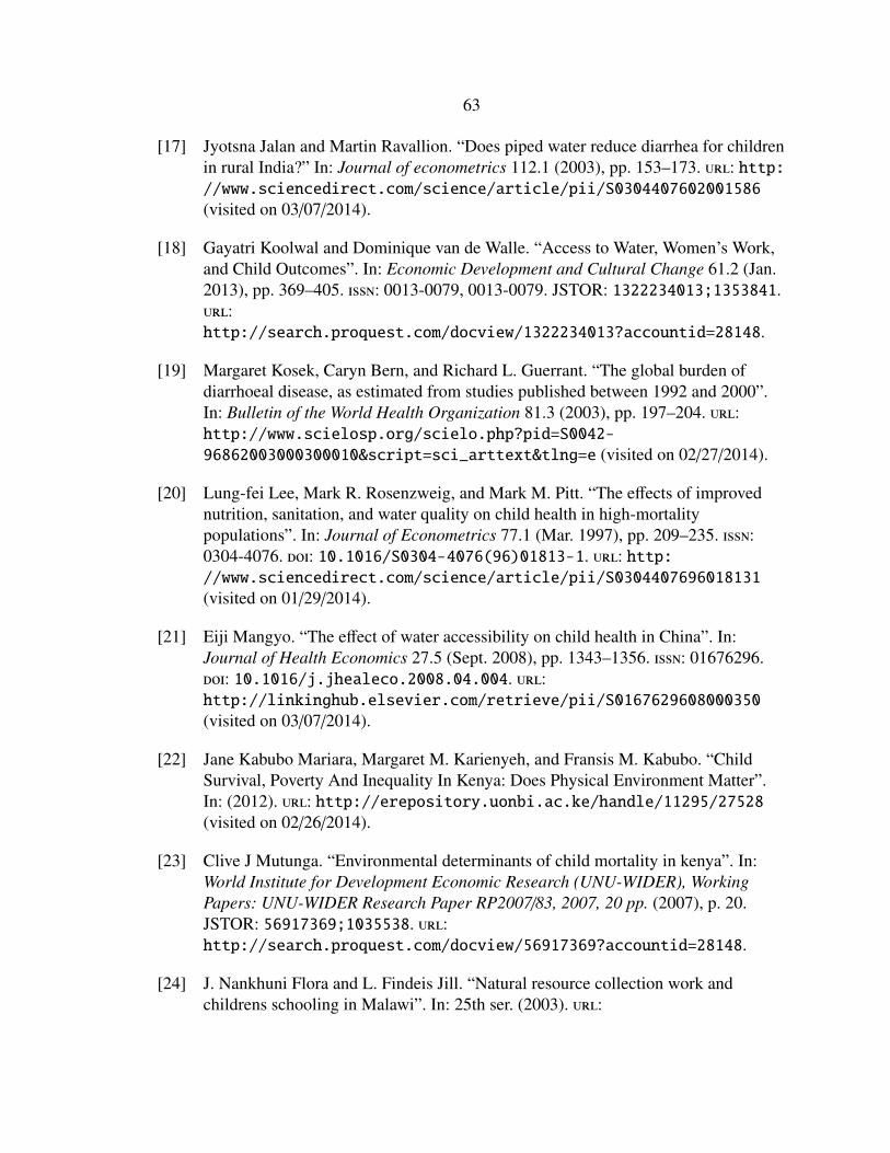
63
[17] Jyotsna Jalan and Martin Ravallion. “Does piped water reduce diarrhea for childrenin rural India?” In: Journal of econometrics 112.1 (2003), pp. 153–173. url: http://www.sciencedirect.com/science/article/pii/S0304407602001586
(visited on 03/07/2014).
[18] Gayatri Koolwal and Dominique van de Walle. “Access to Water, Women’s Work,and Child Outcomes”. In: Economic Development and Cultural Change 61.2 (Jan.2013), pp. 369–405. issn: 0013-0079, 0013-0079. JSTOR: 1322234013;1353841.url:http://search.proquest.com/docview/1322234013?accountid=28148.
[19] Margaret Kosek, Caryn Bern, and Richard L. Guerrant. “The global burden ofdiarrhoeal disease, as estimated from studies published between 1992 and 2000”.In: Bulletin of the World Health Organization 81.3 (2003), pp. 197–204. url:http://www.scielosp.org/scielo.php?pid=S0042-
96862003000300010&script=sci_arttext&tlng=e (visited on 02/27/2014).
[20] Lung-fei Lee, Mark R. Rosenzweig, and Mark M. Pitt. “The effects of improvednutrition, sanitation, and water quality on child health in high-mortalitypopulations”. In: Journal of Econometrics 77.1 (Mar. 1997), pp. 209–235. issn:0304-4076. doi: 10.1016/S0304-4076(96)01813-1. url: http://www.sciencedirect.com/science/article/pii/S0304407696018131
(visited on 01/29/2014).
[21] Eiji Mangyo. “The effect of water accessibility on child health in China”. In:Journal of Health Economics 27.5 (Sept. 2008), pp. 1343–1356. issn: 01676296.doi: 10.1016/j.jhealeco.2008.04.004. url:http://linkinghub.elsevier.com/retrieve/pii/S0167629608000350
(visited on 03/07/2014).
[22] Jane Kabubo Mariara, Margaret M. Karienyeh, and Fransis M. Kabubo. “ChildSurvival, Poverty And Inequality In Kenya: Does Physical Environment Matter”.In: (2012). url: http://erepository.uonbi.ac.ke/handle/11295/27528(visited on 02/26/2014).
[23] Clive J Mutunga. “Environmental determinants of child mortality in kenya”. In:World Institute for Development Economic Research (UNU-WIDER), WorkingPapers: UNU-WIDER Research Paper RP2007/83, 2007, 20 pp. (2007), p. 20.JSTOR: 56917369;1035538. url:http://search.proquest.com/docview/56917369?accountid=28148.
[24] J. Nankhuni Flora and L. Findeis Jill. “Natural resource collection work andchildrens schooling in Malawi”. In: 25th ser. (2003). url:
64
http://ageconsearch.umn.edu/bitstream/25829/1/cp03na01.pdf
(visited on 02/25/2014).
[25] Celine Nauges and Jon Strand. “Water hauling and girls’ school attendance: somenew evidence from Ghana”. In: The World Bank, Policy Research Working PaperSeries: 6443, 2013 (2013). url: http://search.proquest.com/econlit/docview/1361806051/CF56F793083C413BPQ/4?accountid=28148 (visited on02/15/2014).
[26] Menno Pradhan and Laura B. Rawlings. “The Impact and Targeting of SocialInfrastructure Investments: Lessons from the Nicaraguan Social Fund”. In: TheWorld Bank Economic Review 16.2 (2002), pp. 275–295.
[27] Annette Prss-stn and World Health Organization. Safer water, better health costs,benefits and sustainability of interventions to protect and promote health. [Geneva]:World Health Organization, 2008. isbn: 9789241596435 9241596430. url: http://whqlibdoc.who.int/publications/2008/9789241596435_eng.pdf
(visited on 03/31/2014).
[28] George Psacharopoulos. “Child labor versus educational attainment Some evidencefrom Latin America”. In: Journal of population economics 10.4 (1997),pp. 377–386. url:http://link.springer.com/article/10.1007/s001480050049 (visited on03/07/2014).
[29] Sydney Rosen and Jeffrey R. Vincent. “Household Water Resources and RuralProductivity in Sub-Saharan Africa: A Review of the Evidence”. In: HarvardInstitute for International Development (1999). url:http://pdf.usaid.gov/pdf_docs/pnack781.pdf (visited on 03/07/2014).
[30] Carrie L. Shandra, John M. Shandra, and Bruce London. “World bank structuraladjustment, water, and sanitation: A cross-national analysis of child mortality inSub-Saharan Africa”. In: Organization & Environment 24.2 (2011), pp. 107–129.url: http://oae.sagepub.com/content/24/2/107.short (visited on01/27/2015).
[31] James K Tumwine et al. “Diarrhoea and effects of different water sources,sanitation and hygiene behaviour in East Africa”. In: Tropical medicine &
international health: TM & IH 7.9 (Sept. 2002), pp. 750–756. issn: 1360-2276.
[32] USAid. The DHS Program. 2014. url: http://dhsprogram.com/.
[33] James VanDerslice and John Briscoe. “Environmental interventions in developingcountries: interactions and their implications”. In: American journal ofepidemiology 141.2 (1995), pp. 135–144. url:
65
http://aje.oxfordjournals.org/content/141/2/135.short (visited on03/31/2014).
[34] Z S Wang et al. “Reduction of enteric infectious disease in rural China by providingdeep-well tap water”. In: Bulletin of the World Health Organization 67.2 (1989),pp. 171–180. issn: 0042-9686.
[35] Tara Watson. “Public health investments and the infant mortality gap: Evidencefrom federal sanitation interventions on US Indian reservations”. In: Journal ofPublic Economics 90.8 (2006), pp. 1537–1560. url: http://www.sciencedirect.com/science/article/pii/S0047272705001611
(visited on 01/16/2015).
[36] wiseGEEK. What Are Enteric Diseases? (with pictures). wiseGEEK. 2014. url:http://www.wisegeek.com/what-are-enteric-diseases.htm (visited on03/23/2014).

66
APPENDICES

67
APPENDIX A:
MISCELLANEOUS
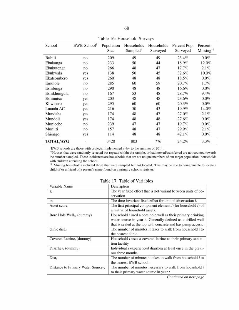
68
Table 16: Household SurveysSchool EWB-School† Population Households Households Percent Pop. Percent
Size Sampled† Surveyed Surveyed Missing††
Buhili no 209 49 49 23.4% 0.0%Ebukanga no 233 50 44 18.9% 12.0%Ebukutenga no 266 48 47 17.7% 2.1%Ebukwala yes 138 50 45 32.6% 10.0%Ekatsombero yes 260 48 48 18.5% 0.0%Emulole no 285 60 59 20.7% 1.7%Eshibinga no 290 48 48 16.6% 0.0%Eshikhungula no 167 53 48 28.7% 9.4%Eshinutsa yes 203 48 48 23.6% 0.0%Khwisero yes 295 60 60 20.3% 0.0%Luanda AC yes 216 50 43 19.9% 14.0%Mundaha yes 174 48 47 27.0% 2.1%Mundoli yes 174 48 48 27.6% 0.0%Munjeche no 239 47 47 19.7% 0.0%Munjiti no 157 48 47 29.9% 2.1%Shiongo yes 114 48 48 42.1% 0.0%
TOTAL/AVG - 3420 803 776 24.2% 3.3%†EWB schools are those with projects implemented prior to the summer of 2014.††Houses that were randomly selected but repeats within the sample, or had moved/transferred are not counted towardsthe number sampled. These incidences are households that are not unique members of our target population: householdswith children attending the school.†††Missing households included those that were sampled but not located. This may be due to being unable to locate achild of or a friend of a parent’s name found on a primary schools register.
Table 17: Table of VariablesVariable Name Descriptionτt The year fixed effect that is not variant between units of ob-
servation.αi The time-invariant fixed effect for unit of observation i.Asset scorei The first principal component element i (for household i) of
a matrix of household assets.Bore Hole Welli,t (dummy) Household i used a bore hole well as their primary drinking
water source in year t. Generally defined as a drilled wellthat is sealed at the top with concrete and has pump access.
clinic dist.i The number of minutes it takes to walk from household i tothe nearest clinic
Covered Latrinei (dummy) Household i uses a covered latrine as their primary sanita-tion facility.
Diarrheai (dummy) Individual i experienced diarrhea at least once in the previ-ous three months
Disti The number of minutes it takes to walk from household i tothe nearest EWB school.
Distance to Primary Water Sourcei,t The number of minutes necessary to walk from household ito their primary water source in year t
Continued on next page
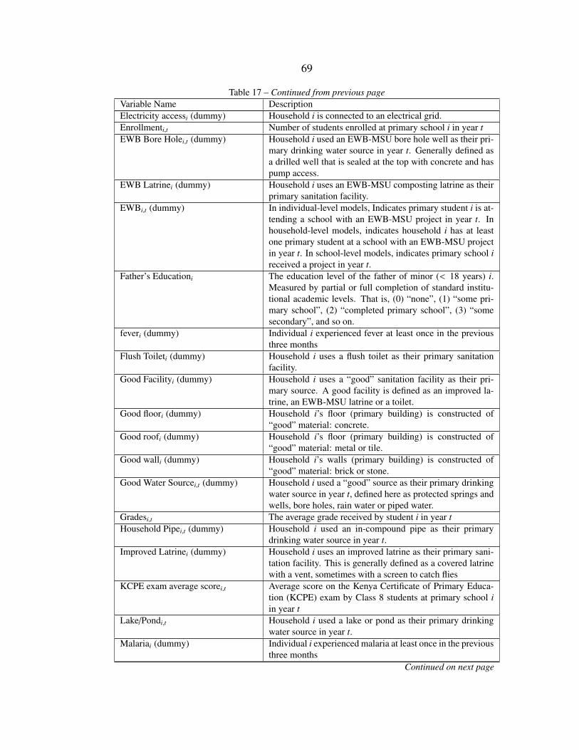
69
Table 17 – Continued from previous pageVariable Name DescriptionElectricity accessi (dummy) Household i is connected to an electrical grid.Enrollmenti,t Number of students enrolled at primary school i in year tEWB Bore Holei,t (dummy) Household i used an EWB-MSU bore hole well as their pri-
mary drinking water source in year t. Generally defined asa drilled well that is sealed at the top with concrete and haspump access.
EWB Latrinei (dummy) Household i uses an EWB-MSU composting latrine as theirprimary sanitation facility.
EWBi,t (dummy) In individual-level models, Indicates primary student i is at-tending a school with an EWB-MSU project in year t. Inhousehold-level models, indicates household i has at leastone primary student at a school with an EWB-MSU projectin year t. In school-level models, indicates primary school ireceived a project in year t.
Father’s Educationi The education level of the father of minor (< 18 years) i.Measured by partial or full completion of standard institu-tional academic levels. That is, (0) “none”, (1) “some pri-mary school”, (2) “completed primary school”, (3) “somesecondary”, and so on.
feveri (dummy) Individual i experienced fever at least once in the previousthree months
Flush Toileti (dummy) Household i uses a flush toilet as their primary sanitationfacility.
Good Facilityi (dummy) Household i uses a “good” sanitation facility as their pri-mary source. A good facility is defined as an improved la-trine, an EWB-MSU latrine or a toilet.
Good floori (dummy) Household i’s floor (primary building) is constructed of“good” material: concrete.
Good roofi (dummy) Household i’s floor (primary building) is constructed of“good” material: metal or tile.
Good walli (dummy) Household i’s walls (primary building) is constructed of“good” material: brick or stone.
Good Water Sourcei,t (dummy) Household i used a “good” source as their primary drinkingwater source in year t, defined here as protected springs andwells, bore holes, rain water or piped water.
Gradesi,t The average grade received by student i in year tHousehold Pipei,t (dummy) Household i used an in-compound pipe as their primary
drinking water source in year t.Improved Latrinei (dummy) Household i uses an improved latrine as their primary sani-
tation facility. This is generally defined as a covered latrinewith a vent, sometimes with a screen to catch flies
KCPE exam average scorei,t Average score on the Kenya Certificate of Primary Educa-tion (KCPE) exam by Class 8 students at primary school iin year t
Lake/Pondi,t Household i used a lake or pond as their primary drinkingwater source in year t.
Malariai (dummy) Individual i experienced malaria at least once in the previousthree months
Continued on next page
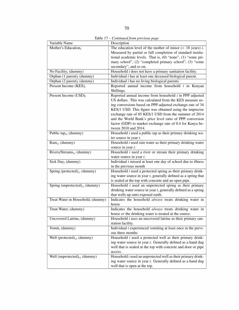
70
Table 17 – Continued from previous pageVariable Name DescriptionMother’s Educationi The education level of the mother of minor (< 18 years) i.
Measured by partial or full completion of standard institu-tional academic levels. That is, (0) “none”, (1) “some pri-mary school”, (2) “completed primary school”, (3) “somesecondary”, and so on.
No Facilityi (dummy) Household i does not have a primary sanitation facility.Orphan (1 parent)i (dummy) Individual i has at least one deceased biological parent.Orphan (2 parent)i (dummy) Individual i has no living biological parents.Present Income (KES)i Reported annual income from household i in Kenyan
Shillings.Present Income (USD)i Reported annual income from household i in PPP adjusted
US dollars. This was calculated from the KES measure us-ing conversions based on PPP-adjusted exchange rate of 34KES/1 USD. This figure was obtained using the impreciseexchange rate of 85 KES/1 USD from the summer of 2014and the World Bank’s price level ratio of PPP conversionfactor (GDP) to market exchange rate of 0.4 for Kenya be-tween 2010 and 2014.
Public tapi,t (dummy) Household i used a public tap as their primary drinking wa-ter source in year t.
Raini,t (dummy) Household i used rain water as their primary drinking watersource in year t.
Rivers/Streamsi,t (dummy) Household i used a river or stream their primary drinkingwater source in year t.
Sick Dayi (dummy) Individual i missed at least one day of school due to illnessin the previous month
Spring (protected)i,t (dummy) Household i used a protected spring as their primary drink-ing water source in year t, generally defined as a spring thatis sealed at the top with concrete and an open pipe.
Spring (unprotected)i,t (dummy) Household i used an unprotected spring as their primarydrinking water source in year t, generally defined as a springthat wells up onto exposed earth.
Treat Water in Householdi (dummy) Indicates the household always treats drinking water inhouse
Treat Wateri (dummy) Indicates the household always treats drinking water inhouse or the drinking water is treated at the source.
Uncovered Latrinei (dummy) Household i uses an uncovered latrine as their primary san-itation facility.
Vomiti (dummy) Individual i experienced vomiting at least once in the previ-ous three months
Well (protected)i,t (dummy) Household i used a protected well as their primary drink-ing water source in year t. Generally defined as a hand dugwell that is sealed at the top with concrete and door or pipeaccess.
Well (unprotected)i,t (dummy) Household i used an unprotected well as their primary drink-ing water source in year t. Generally defined as a hand dugwell that is open at the top.

71
APPENDIX B
AUXILLARY REGRESSION RESULTS
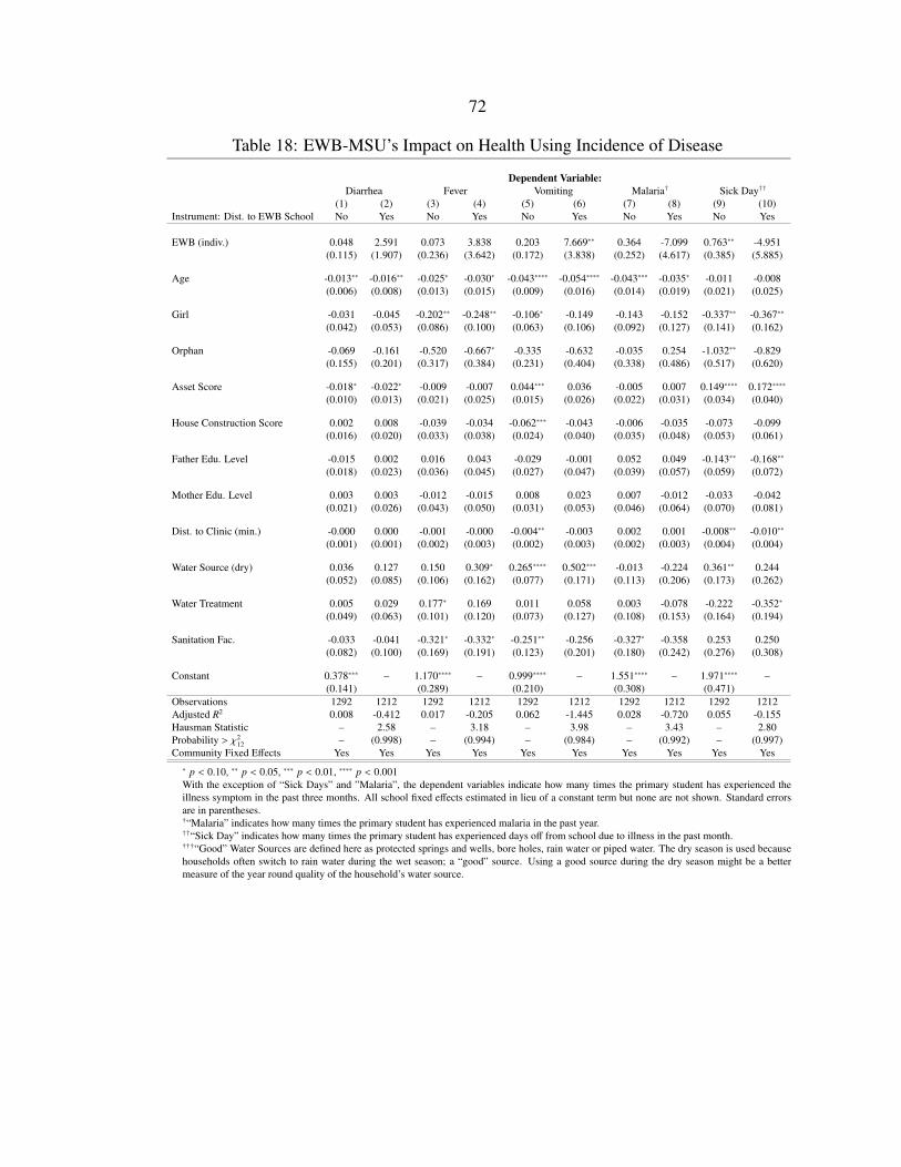
72
Table 18: EWB-MSU’s Impact on Health Using Incidence of Disease
Dependent Variable:Diarrhea Fever Vomiting Malaria† Sick Day††
(1) (2) (3) (4) (5) (6) (7) (8) (9) (10)Instrument: Dist. to EWB School No Yes No Yes No Yes No Yes No Yes
EWB (indiv.) 0.048 2.591 0.073 3.838 0.203 7.669∗∗ 0.364 -7.099 0.763∗∗ -4.951(0.115) (1.907) (0.236) (3.642) (0.172) (3.838) (0.252) (4.617) (0.385) (5.885)
Age -0.013∗∗ -0.016∗∗ -0.025∗ -0.030∗ -0.043∗∗∗∗ -0.054∗∗∗∗ -0.043∗∗∗ -0.035∗ -0.011 -0.008(0.006) (0.008) (0.013) (0.015) (0.009) (0.016) (0.014) (0.019) (0.021) (0.025)
Girl -0.031 -0.045 -0.202∗∗ -0.248∗∗ -0.106∗ -0.149 -0.143 -0.152 -0.337∗∗ -0.367∗∗
(0.042) (0.053) (0.086) (0.100) (0.063) (0.106) (0.092) (0.127) (0.141) (0.162)
Orphan -0.069 -0.161 -0.520 -0.667∗ -0.335 -0.632 -0.035 0.254 -1.032∗∗ -0.829(0.155) (0.201) (0.317) (0.384) (0.231) (0.404) (0.338) (0.486) (0.517) (0.620)
Asset Score -0.018∗ -0.022∗ -0.009 -0.007 0.044∗∗∗ 0.036 -0.005 0.007 0.149∗∗∗∗ 0.172∗∗∗∗
(0.010) (0.013) (0.021) (0.025) (0.015) (0.026) (0.022) (0.031) (0.034) (0.040)
House Construction Score 0.002 0.008 -0.039 -0.034 -0.062∗∗∗ -0.043 -0.006 -0.035 -0.073 -0.099(0.016) (0.020) (0.033) (0.038) (0.024) (0.040) (0.035) (0.048) (0.053) (0.061)
Father Edu. Level -0.015 0.002 0.016 0.043 -0.029 -0.001 0.052 0.049 -0.143∗∗ -0.168∗∗
(0.018) (0.023) (0.036) (0.045) (0.027) (0.047) (0.039) (0.057) (0.059) (0.072)
Mother Edu. Level 0.003 0.003 -0.012 -0.015 0.008 0.023 0.007 -0.012 -0.033 -0.042(0.021) (0.026) (0.043) (0.050) (0.031) (0.053) (0.046) (0.064) (0.070) (0.081)
Dist. to Clinic (min.) -0.000 0.000 -0.001 -0.000 -0.004∗∗ -0.003 0.002 0.001 -0.008∗∗ -0.010∗∗
(0.001) (0.001) (0.002) (0.003) (0.002) (0.003) (0.002) (0.003) (0.004) (0.004)
Water Source (dry) 0.036 0.127 0.150 0.309∗ 0.265∗∗∗∗ 0.502∗∗∗ -0.013 -0.224 0.361∗∗ 0.244(0.052) (0.085) (0.106) (0.162) (0.077) (0.171) (0.113) (0.206) (0.173) (0.262)
Water Treatment 0.005 0.029 0.177∗ 0.169 0.011 0.058 0.003 -0.078 -0.222 -0.352∗
(0.049) (0.063) (0.101) (0.120) (0.073) (0.127) (0.108) (0.153) (0.164) (0.194)
Sanitation Fac. -0.033 -0.041 -0.321∗ -0.332∗ -0.251∗∗ -0.256 -0.327∗ -0.358 0.253 0.250(0.082) (0.100) (0.169) (0.191) (0.123) (0.201) (0.180) (0.242) (0.276) (0.308)
Constant 0.378∗∗∗ – 1.170∗∗∗∗ – 0.999∗∗∗∗ – 1.551∗∗∗∗ – 1.971∗∗∗∗ –(0.141) (0.289) (0.210) (0.308) (0.471)
Observations 1292 1212 1292 1212 1292 1212 1292 1212 1292 1212Adjusted R2 0.008 -0.412 0.017 -0.205 0.062 -1.445 0.028 -0.720 0.055 -0.155Hausman Statistic – 2.58 – 3.18 – 3.98 – 3.43 – 2.80Probability > χ2
12 – (0.998) – (0.994) – (0.984) – (0.992) – (0.997)Community Fixed Effects Yes Yes Yes Yes Yes Yes Yes Yes Yes Yes∗ p < 0.10, ∗∗ p < 0.05, ∗∗∗ p < 0.01, ∗∗∗∗ p < 0.001With the exception of “Sick Days” and ”Malaria”, the dependent variables indicate how many times the primary student has experienced theillness symptom in the past three months. All school fixed effects estimated in lieu of a constant term but none are not shown. Standard errorsare in parentheses.†“Malaria” indicates how many times the primary student has experienced malaria in the past year.††“Sick Day” indicates how many times the primary student has experienced days off from school due to illness in the past month.†††“Good” Water Sources are defined here as protected springs and wells, bore holes, rain water or piped water. The dry season is used becausehouseholds often switch to rain water during the wet season; a “good” source. Using a good source during the dry season might be a bettermeasure of the year round quality of the household’s water source.

73
APPENDIX C
THE EXPERIMENTAL IDEAL
74
The Ideal Data
EWB-MSU seeks to improve the welfare of children attending primary school.
Accordingly, the ideal data would provide information at the individual-level on children
at Khwisero primary schools over a period of time. It is expected that EWB-MSU projects
improve the safety of the school childrens’ water source. Thus, one would collect health
data on Khwisero students’ water borne illness morbidity such as typhoid and diarrhea. It
is expected that healthier students are able to increase school attendance and performance.
Thus, one would collect education records on individual students such as grades, exam
scores, and attendance records. It is expected that EWB-MSU’s water projects reduce
water collection times for students while at school. Thus, one would collect data on the
students’ water collection labor. It is expected that EWB-MSU projects raise the students’
aspirations for their future via interactions with collegiate foreigners and demonstration of
welfare improvements through collective action. Thus, one would collect data on what
these students’ aspire to achieve academically, professionally and socio-politically in the
future. In addition, one would collect individual-level information on other known
covariates that related to the enumerated welfare outcomes. These might include the
student’s household wealth and parental education levels. Doing so will allow the removal
variation explained by these other factors and increase the precision of estimates in the
econometric analysis of these data.
The Experimental Ideal
The ideal experiment to test the welfare impacts of EWB-MSU would randomly
assign students to schools with or without EWB-MSU projects. A “treatment” group of
students would attend a school that receives a project, while a “control” group would not.
The ideal data described would be collected from all “treatment” and “control” individuals
and their families.
75
yi = α + δEWBi + xiβ + εi
Random assignment would remove the possibility of selection bias in community
characteristics and bias from choice in attendance of EWB schools. Therefore, the effect
of EWB-MSU on the outcome of interest, yi, may be interpreted as causal. From the ideal
data, a conditioning set, xi, may be used to increase estimate precision but is not necessary
for estimating a causal effect.