Marine Geology 345 (2013) 96–112

Contents lists available at ScienceDirect

Marine Geology

j ourna l homepage: www.e lsev ie r .com/ locate /margeo

The use of modeling and suspended sediment concentrationmeasurements for quantifying net suspended sediment transportthrough a large tidally dominated inlet

Li H. Erikson a,⁎, Scott A. Wright b, Edwin Elias c, Daniel M. Hanes d, David H. Schoellhamer b, John Largier e

a U.S. Geological Survey, Pacific Coastal and Marine Science Center, Santa Cruz, CA, USAb U.S. Geological Survey, California Water Science Center, Sacramento, CA, USAc Deltares, Delft, Netherlandsd Saint Louis University, Dept. of Earth and Atmospheric Sciences, MO, USAe U.C. Davis Bodega Marine Laboratories, Bodega Bay, CA, USA

⁎ Corresponding author. Tel.: +1 831 460 7563.E-mail address: lerikson@usgs.gov (L.H. Erikson).

0025-3227/$ – see front matter. Published by Elsevier Bhttp://dx.doi.org/10.1016/j.margeo.2013.06.001

a b s t r a c t

a r t i c l e i n f o

Article history:Received 12 July 2012Received in revised form 28 May 2013Accepted 3 June 2013Available online 13 June 2013

Keywords:inlet sediment fluxsuspended sediment transportestuariesDelft3DSan Francisco Bay

Sediment exchange at large energetic inlets is often difficult to quantify due complex flows, massive amountsof water and sediment exchange, and environmental conditions limiting long-term data collection. In aneffort to better quantify such exchange this study investigated the use of suspended sediment concentrations(SSC) measured at an offsite location as a surrogate for sediment exchange at the tidally dominated GoldenGate inlet in San Francisco, CA. A numerical model was calibrated and validated against water and suspendedsediment flux measured during a spring–neap tide cycle across the Golden Gate. The model was then run forfive months and net exchange was calculated on a tidal time-scale and compared to SSC measurements at theAlcatraz monitoring site located in Central San Francisco Bay ~5 km from the Golden Gate. Numericallymodeled tide averaged flux across the Golden Gate compared well (r2 = 0.86, p-value b0.05) with 25 hlow-pass filtered (tide averaged) SSCs measured at Alcatraz over the five month simulation period (Januarythrough April 2008). This formed a basis for the development of a simple equation relating the advective fluxat Alcatraz with suspended sediment flux across the Golden Gate. Utilization of the equation with allavailable Alcatraz SSC data resulted in an average export rate of 1.2 Mt/yr during water years 2004 through2010. While the rate is comparable to estimated suspended sediment inflow rates from sources within theBay over the same time period (McKee et al., 2013-this issue), there was little variation from year to year.Exports were computed to be greatest during the wettest water year analyzed but only marginally so.

Published by Elsevier B.V.

1. Introduction

Large tidal estuaries located at the interface between rivers and theocean provide awealth of natural resources and are often an economichub in many parts of the world. A quantitative understanding of sedi-ment delivered to, stored within, and exported from an estuary isimportant for a number of issues including maintenance dredging ofnavigation channels, sand mining, light availability for primaryproductivity, creation and sustainability of tidal wetlands, and thetransport of particle-bound nutrients and contaminants (Teeter etal., 1996; Zedler and Callaway, 2001). Although an estuary providesa readily definable control volume where point sources and sinksexist in the form of rivers and the open ocean, it is difficult todetermine sediment influx to the system and net flux at the estuary–ocean boundary. This is particularly true for large tidal inlets inregions of modest to high tide ranges where it is not physically or

.V.

economically feasible to continuously monitor sediment flux, andexchange is complicated by variations in bathymetry, topography,and density driven flows.

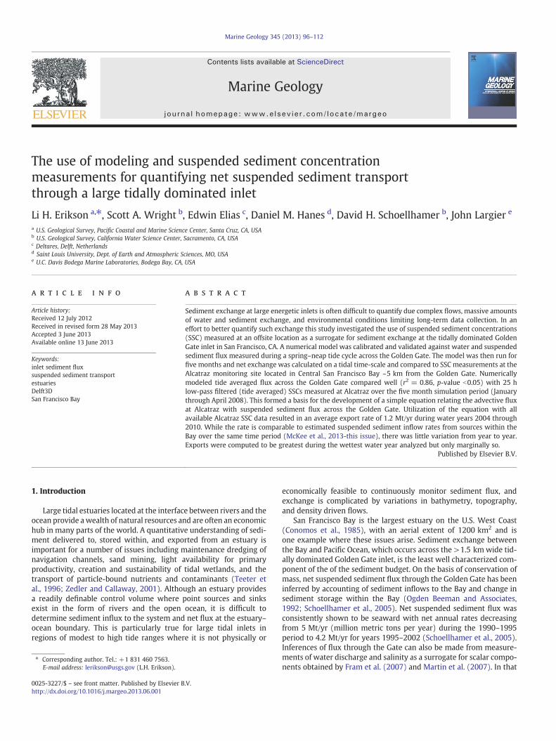
San Francisco Bay is the largest estuary on the U.S. West Coast(Conomos et al., 1985), with an aerial extent of 1200 km2 and isone example where these issues arise. Sediment exchange betweenthe Bay and Pacific Ocean, which occurs across the >1.5 km wide tid-ally dominated Golden Gate inlet, is the least well characterized com-ponent of the of the sediment budget. On the basis of conservation ofmass, net suspended sediment flux through the Golden Gate has beeninferred by accounting of sediment inflows to the Bay and change insediment storage within the Bay (Ogden Beeman and Associates,1992; Schoellhamer et al., 2005). Net suspended sediment flux wasconsistently shown to be seaward with net annual rates decreasingfrom 5 Mt/yr (million metric tons per year) during the 1990–1995period to 4.2 Mt/yr for years 1995–2002 (Schoellhamer et al., 2005).Inferences of flux through the Gate can also be made from measure-ments of water discharge and salinity as a surrogate for scalar compo-nents obtained by Fram et al. (2007) and Martin et al. (2007). In that

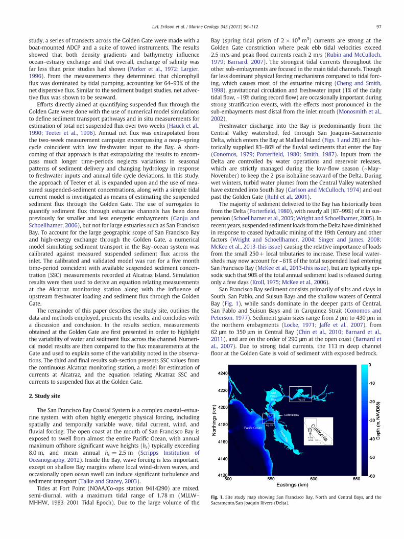
Fig. 1. Site study map showing San Francisco Bay, North and Central Bays, and theSacramento/San Joaquin Rivers (Delta).

97L.H. Erikson et al. / Marine Geology 345 (2013) 96–112

study, a series of transects across the Golden Gate were made with aboat-mounted ADCP and a suite of towed instruments. The resultsshowed that both density gradients and bathymetry influenceocean–estuary exchange and that overall, exchange of salinity wasfar less than prior studies had shown (Parker et al., 1972; Largier,1996). From the measurements they determined that chlorophyllflux was dominated by tidal pumping, accounting for 64–93% of thenet dispersive flux. Similar to the sediment budget studies, net advec-tive flux was shown to be seaward.

Efforts directly aimed at quantifying suspended flux through theGolden Gate were done with the use of numerical model simulationsto define sediment transport pathways and in situ measurements forestimation of total net suspended flux over two weeks (Hauck et al.,1990; Teeter et al., 1996). Annual net flux was extrapolated fromthe two-week measurement campaign encompassing a neap–springcycle coincident with low freshwater input to the Bay. A short-coming of that approach is that extrapolating the results to encom-pass much longer time-periods neglects variations in seasonalpatterns of sediment delivery and changing hydrology in responseto freshwater inputs and annual tide cycle deviations. In this study,the approach of Teeter et al. is expanded upon and the use of mea-sured suspended-sediment concentrations, along with a simple tidalcurrent model is investigated as means of estimating the suspendedsediment flux through the Golden Gate. The use of surrogates toquantify sediment flux through estuarine channels has been donepreviously for smaller and less energetic embayments (Ganju andSchoellhamer, 2006), but not for large estuaries such as San FranciscoBay. To account for the large geographic scope of San Francisco Bayand high-energy exchange through the Golden Gate, a numericalmodel simulating sediment transport in the Bay–ocean system wascalibrated against measured suspended sediment flux across theinlet. The calibrated and validated model was run for a five monthtime-period coincident with available suspended sediment concen-tration (SSC) measurements recorded at Alcatraz Island. Simulationresults were then used to derive an equation relating measurementsat the Alcatraz monitoring station along with the influence ofupstream freshwater loading and sediment flux through the GoldenGate.

The remainder of this paper describes the study site, outlines thedata and methods employed, presents the results, and concludes witha discussion and conclusion. In the results section, measurementsobtained at the Golden Gate are first presented in order to highlightthe variability of water and sediment flux across the channel. Numeri-cal model results are then compared to the flux measurements at theGate and used to explain some of the variability noted in the observa-tions. The third and final results sub-section presents SSC values fromthe continuous Alcatraz monitoring station, a model for estimation ofcurrents at Alcatraz, and the equation relating Alcatraz SSC andcurrents to suspended flux at the Golden Gate.

2. Study site

The San Francisco Bay Coastal System is a complex coastal–estua-rine system, with often highly energetic physical forcing, includingspatially and temporally variable wave, tidal current, wind, andfluvial forcing. The open coast at the mouth of San Francisco Bay isexposed to swell from almost the entire Pacific Ocean, with annualmaximum offshore significant wave heights (hs) typically exceeding8.0 m, and mean annual hs = 2.5 m (Scripps Institution ofOceanography, 2012). Inside the Bay, wave forcing is less important,except on shallow Bay margins where local wind-driven waves, andoccasionally open ocean swell can induce significant turbulence andsediment transport (Talke and Stacey, 2003).

Tides at Fort Point (NOAA/Co-ops station 9414290) are mixed,semi-diurnal, with a maximum tidal range of 1.78 m (MLLW–

MHHW, 1983–2001 Tidal Epoch). Due to the large volume of the

Bay (spring tidal prism of 2 × 109 m3) currents are strong at theGolden Gate constriction where peak ebb tidal velocities exceed2.5 m/s and peak flood currents reach 2 m/s (Rubin and McCulloch,1979; Barnard, 2007). The strongest tidal currents throughout theother sub-embayments are focused in the main tidal channels. Thoughfar less dominant physical forcing mechanisms compared to tidal forc-ing, which causes most of the estuarine mixing (Cheng and Smith,1998), gravitational circulation and freshwater input (1% of the dailytidal flow, ~19% during record flow) are occasionally important duringstrong stratification events, with the effects most pronounced in thesub-embayments most distal from the inlet mouth (Monosmith et al.,2002).

Freshwater discharge into the Bay is predominantly from theCentral Valley watershed, fed through San Joaquin–SacramentoDelta, which enters the Bay at Mallard Island (Figs. 1 and 2B) and his-torically supplied 83–86% of the fluvial sediments that enter the Bay(Conomos, 1979; Porterfield, 1980; Smith, 1987). Inputs from theDelta are controlled by water operations and reservoir releases,which are strictly managed during the low-flow season (~May–November) to keep the 2-psu isohaline seaward of the Delta. Duringwet winters, turbid water plumes from the Central Valley watershedhave extended into South Bay (Carlson and McCulloch, 1974) and outpast the Golden Gate (Ruhl et al., 2001).

The majority of sediment delivered to the Bay has historically beenfrom the Delta (Porterfield, 1980), with nearly all (87–99%) of it in sus-pension (Schoellhamer et al., 2005;Wright and Schoellhamer, 2005). Inrecent years, suspended sediment loads from theDelta have diminishedin response to ceased hydraulic mining of the 19th Century and otherfactors (Wright and Schoellhamer, 2004; Singer and James, 2008;McKee et al., 2013-this issue) causing the relative importance of loadsfrom the small 250+ local tributaries to increase. These local water-sheds may now account for ~61% of the total suspended load enteringSan Francisco Bay (McKee et al., 2013-this issue), but are typically epi-sodic such that 90% of the total annual sediment load is released duringonly a few days (Kroll, 1975; McKee et al., 2006).

San Francisco Bay sediment consists primarily of silts and clays inSouth, San Pablo, and Suisun Bays and the shallow waters of CentralBay (Fig. 1), while sands dominate in the deeper parts of Central,San Pablo and Suisun Bays and in Carquinez Strait (Conomos andPeterson, 1977). Sediment grain sizes range from 2 μm to 430 μm inthe northern embayments (Locke, 1971; Jaffe et al., 2007), from62 μm to 350 μm in Central Bay (Chin et al., 2010; Barnard et al.,2011), and are on the order of 290 μm at the open coast (Barnard etal., 2007). Due to strong tidal currents, the 113 m deep channelfloor at the Golden Gate is void of sediment with exposed bedrock.

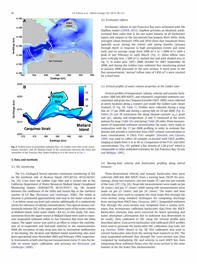
Fig. 2. Studied areas of suspended sediment flux; (A) Golden Gate inlet at the ocean–estuary interface, and (B) Mallard Island at the constriction between the Delta andremainder of San Francisco Bay. Depth shading in A is the same as in Fig. 1.

98 L.H. Erikson et al. / Marine Geology 345 (2013) 96–112

3. Data and methods

3.1. SSC monitoring

The U.S. Geological Survey operates continuous monitoring of SSCon the northeast side of Alcatraz Island (N37.82722, W122.42167;Fig. 2A) 5 km from the Golden Gate inlet and a second one at theCalifornia Department of Water Resources Mallard Island ComplianceMonitoring Station (N38.042778, W121.91917; Fig. 2B) locatedbetween the confluence of the Delta and Suisun Bay in the northernreaches of S.F. Bay (Buchanan and Lionberger, 2006). The sonde atAlcatraz is positioned approximately mid-way in the water column at~3 m below mean sea level and consists additionally of a conductivitysensor for inference of salinity concentrations. Two optical sensors con-tinuouslymonitor SSC in the upper and lower parts of thewater columnat Mallard Island (total water depth ~8.8 m). In this study, SSC mea-surements from the upper sensor at Mallard Island were used to repre-sent suspended sediment influx to San Francisco Bay from the Deltaregion. The upper sensor was used in an effort to reduce the contribu-tion of re-suspended and bed-load material in the measurements.With the exception of data drop-outs due to instrument malfunctionor bio-fouling, the Alcatraz and Mallard Island monitoring sites havebeen operational since November 2003 and February 1994, respective-ly. Instruments at both sites log onemeasurement every 15 min. For de-tails on sensor types, calibration, and accuracy see Buchanan andLionberger (2006).

3.2. Freshwater inflows

Freshwater inflows to San Francisco Bay were estimated with theDayflow model (CDWR, 2012). Dayflow provides an idealized, unidi-rectional flow value that is the net water balance of all freshwaterinputs and outputs to the Sacramento/San Joaquin River Delta. Dailyaveraged values between 1956 and 2010 show that maximum flowstypically occur during the winter and spring months (Januarythrough April) in response to high precipitation events and snowmelt, and on average range from 1000 m3/s to >2000 m3/s with apeak in late February to early March (Fig. 3). Delta inflow rateswere critically low (~500 m3/s; dashed line and dark shaded area inFig. 3) in water year (WY) 2008, October 01 2007–September 302008, and during the Golden Gate sediment flux monitoring periodin January 2008 discussed in the next section. A week prior to theflux measurements, ‘normal’ inflow rates of 1450 m3/s were reachedfor a brief time.

3.3. Vertical profiles of water column properties at the Golden Gate

Vertical profiles of temperature, salinity, velocity and acoustic back-scatter (600 kHz RDI ADCP), and volumetric suspended-sediment con-centration and grain size (Sequoia Scientific LISST-100X)were collectedat seven locations along a transect just inside the Golden Gate (InnerTransect, IT, Fig. 2A, Table 1). Profiles were collected during a neaptide on 17 Jan 2008 and during a spring tide on 24 Jan 2008 (Fig. 4).Tables 2A and 2B summarize the along channel currents (uac), grainsize (gs), salinity, and temperature (S and T) measured at the sevenstations for neap (Table 2A) and spring (Table 2B) tides. Pointmeasure-ments of suspended-sediment concentration (by mass) were made inconjunction with the 17 Jan 2008 profiling in order to estimate flocdensity and provide a conversion from LISST volume concentration tomass concentration. A USGS P-61 sampler (Edwards and Glysson,1999) was used to collect 20 samples co-located with LISST profiles,ranging in depth from 3 m to 30 m. Comparison of the P-61 and LISSTconcentrations (Fig. 5A) yielded a floc density of 1.26 g/cm3 which iscomparable to other published estimates for San Francisco Bay (Krankand Milligan, 1992).

3.4. Moving-boat velocity and backscatter profiling along lateraltransects

Three-dimensional velocity and acoustic backscatter data werecollected (600 kHz RDI ADCP) from a moving boat (DGPS for posi-tioning) along two transects, one just inside (IT) and one just outsideof the Gate (OT) (Fig. 2A). Neap tide measurements were made on Jan16 (outer) and Jan 17 (inner) while spring tide measurements weremade on Jan 23 (outer) and Jan 24 (inner). The water and boatvelocity data were used to compute the total water flux through thecross-section using standard techniques for computing dischargefrom moving-boat ADCP data (Simpson, 2001). Suspended-sedimentflux through the cross-section was computed from a similar tech-nique that incorporates calibrated backscatter data from the ADCP.Backscatter intensity data were corrected for beam spreading andwater absorption (attenuation due to sediment was determined tobe small), then calibrated to SSC using the vertical profile datadescribed above. Concurrent backscatter and calibrated LISST profileswere used to generate the backscatter-SSC calibration (log scale, seee.g. Gartner, 2004) shown in Fig. 5B. This calibration was used toconvert backscatter data from the moving boat transects to SSC. Thetotal suspended-sediment flux through the cross-section was thencomputed by multiplying SSC and velocity in each ADCP bin, thenintegrating these sediment fluxes over the cross-section in the samemanner as for the water flux measurements.

Fig. 3. Net freshwater inflows from the Sacramento/San Joaquin River Delta to San Francisco Bay (California Department of Water Resources, 2012). Darker gray area highlights thetime-period in water year (WY) 2008 when flux measurements at the Golden Gate were obtained for this study; lighter gray shading indicates time-period of model simulation.Compared to the long-term mean (solid line), freshwater inputs were low during the flux measurements.

99L.H. Erikson et al. / Marine Geology 345 (2013) 96–112

3.5. Numerical modeling

Suspended sediment flux measurements obtained in January 2008(Sections 3.3 and 3.4) coincided with relatively low seas and swell(max significant wave heights = 2.5 m at the SF Bar buoy, CDIP)and calm meteorological conditions (max winds b 5 m/s, NDBC)and hence only tidal forcing, freshwater, and sediment inputs wereused as boundary conditions to model sediment flux through theGolden Gate.

The numerical model Delft3D was used to simulate water andsediment exchange at the Golden Gate (Lesser et al., 2004; Deltares,2011). The Delft3D package is a modeling system that consists of anumber of integrated modules; the ones relevant to this work allowfor the simulation of hydrodynamic flow by solving the shallowwater equations, and transport of salinity and sediment by solvingthe advection–diffusion equation.

Given the large spatial extent of the San Francisco Bay system, themodel was divided into five two-way coupled domains of varying res-olution thus enabling parallel computing and reducing computationtime (Fig. 6). Grid resolution ranged from ~50 to 100 m at the GoldenGate inlet and from 100 m to >500 m in the northern reaches ofSuisun Bay The Delta was highly schematized as the primary goalwas to provide storage of the tidal prism. Tidal variations were drivenat the open boundaries of the large-scale ocean domain that extendedout past the continental shelf. A total of 12 tidal constituent ampli-tudes and phases (M2, S2, N2, K2, K1, O1, P1, Q1, MF, MM, M4, MS4,and MN4) were applied at the open boundary with initial estimatesobtained from the TOPEX7.2 global tidal model (Egbert et al., 1994;Egbert and Erofeeva, 2002). Hydrodynamic aspects of the modelwere calibrated and validated against >30 tide stations throughoutthe Bay and water flux measurements obtained along the inner andouter transects across the Golden Gate described previously. Detailsof the numerical modeling approach used in this study, includinghydrodynamic model calibration and validation, can be found inElias and Hansen (2012).

All domains were run in a depth averaged mode (2DH). Thisapproach assumes that flows at the Golden Gate and all other areasare vertically well-mixed and not strongly stratified; a reasonable as-sumption given that the model simulations were done for a critically

Table 1Location and water depth at stations sampled along the inner transect (IT).

Station ID Lon Lat Water depth(DD) (DD) (m)

IT1 −122.47126 37.83215 32.5IT2 −122.47064 37.82814 51.9IT3 −122.46781 37.82580 57.1IT4 −122.46712 37.82309 56.5IT5 −122.46621 37.81988 50.5IT6 −122.46843 37.81651 34.9IT7 −122.47033 37.81450 30.9

dry water year and that there was little vertical variation in measuredsalinity. If the water column was actually strongly stratified then the2D model would presumably have significant discrepancies in thepredicted fields of both velocity and suspended sediment concentra-tion. Typically the vertical velocity gradients would be larger for strat-ified flows, and the suspended sediment distribution could influencedby flocculation processes if there was a sharp interface between freshand brackish water.

Four sediment fractions were simulated in the model; twonon-cohesive (sand) and two cohesive. Based on measured grain sizedistributions at the Golden Gate and previous measurements withinCentral Bay and outer coast, median sand-sized particles of 200 μmand 350 μm were simulated. A specific density of 2650 kg/m3 and drybed density of 1600 kg/m3 was assumed for all sand fractions; all sandtransport calibration parameters were kept at the default values. Sandfraction transport was modeled with the van Rijn TR2004 formulation,which has been shown to successfully represent the movement ofnon-cohesive sediment ranging in size from 60 μm to 600 μm (VanRijn, 2007).

Transport of the cohesive mud fractions were modeled with theKrone and Ariathurai–Partheniades formulations (Krone, 1962;Ariathurai, 1974). The critical shear stress for deposition (τcrd)was set to 1000 N/m2, which effectively implied that deposition was afunction only of concentration and fall velocity (Wintwerp and VanKesteren, 2004). The critical shear stress for erosion (τcre), fall speed ve-locity (ws), and erosion rate constants (M) were treated as calibration pa-rameters. Values in the range of 0.1 N/m2 b τcre b 0.4 N/m2, 0.09 mm/s bw b 1.01 mm/s, and 5 · 10−5 kg/m2/s b M b 2 · 10−4 kg/m2/s weretested based on previous laboratory and modeling studies (Mehta,1986; Teeter, 1986; Kineke and Sternberg, 1989; Krank and Milligan,1992; Ganju and Schoellhamer, 2009; van der Wegen et al., 2011a,b).Characteristic parameters of the mud fractions were determined by run-ning numerous simulations with varying sediment size and minimizingobserved–modeled differences; the resulting parameters are listed inTable 3. A mid-range dry bed density of 850 kg/m3 was assigned toboth cohesive fractions (Porterfield, 1980). Based on recent fieldmeasurements (Manning and Schoellhamer, 2013-this issue), fall speedvelocitieswere kept constant under all salinity concentrations and floccu-lation was considered to be negligible.

Bed composition maps were generated following guidelinesoutlined by van der Wegen et al. (2011a,b). In that approach, initialbed composition is estimated by defining sediment availabilitythroughout the domain and then running the model over long timeperiods to distribute sediments over the domain using prevailinghydrodynamic conditions. The resulting bed composition is thenused as the initial condition. In this study, bed thickness maps wereconstructed from measurements summarized by Chin et al. (2004)and assuming 6 m in areas void of observations. A single layer wasused, such that all fractions eroded and deposited onto the samelayer. Initial estimates of bed composition were assumed to consistof 100% sand in the ocean domain and at the Golden Gate inlet, 6%cohesive and 94% sand in Central Bay and central channels of north

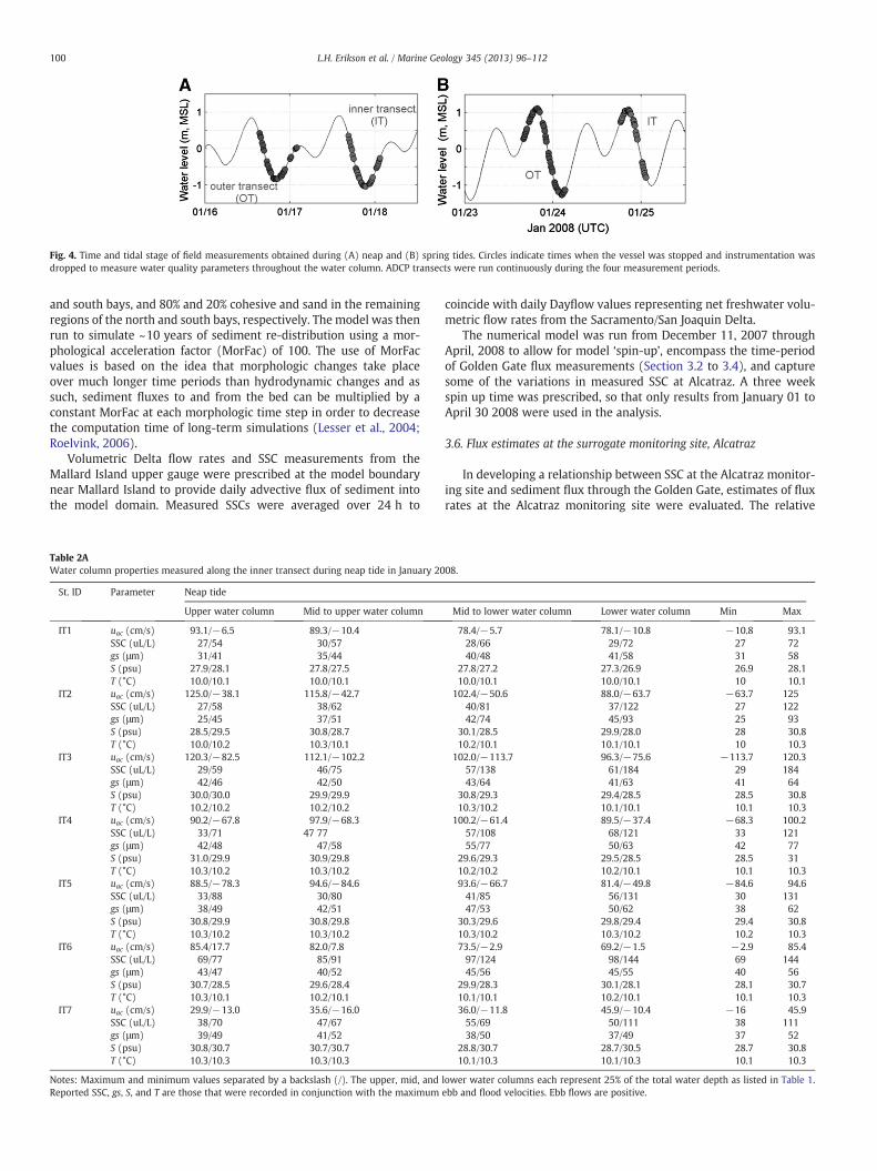
Fig. 4. Time and tidal stage of field measurements obtained during (A) neap and (B) spring tides. Circles indicate times when the vessel was stopped and instrumentation wasdropped to measure water quality parameters throughout the water column. ADCP transects were run continuously during the four measurement periods.

100 L.H. Erikson et al. / Marine Geology 345 (2013) 96–112

and south bays, and 80% and 20% cohesive and sand in the remainingregions of the north and south bays, respectively. The model was thenrun to simulate ~10 years of sediment re-distribution using a mor-phological acceleration factor (MorFac) of 100. The use of MorFacvalues is based on the idea that morphologic changes take placeover much longer time periods than hydrodynamic changes and assuch, sediment fluxes to and from the bed can be multiplied by aconstant MorFac at each morphologic time step in order to decreasethe computation time of long-term simulations (Lesser et al., 2004;Roelvink, 2006).

Volumetric Delta flow rates and SSC measurements from theMallard Island upper gauge were prescribed at the model boundarynear Mallard Island to provide daily advective flux of sediment intothe model domain. Measured SSCs were averaged over 24 h to

Table 2AWater column properties measured along the inner transect during neap tide in January 20

St. ID Parameter Neap tide

Upper water column Mid to upper water column

IT1 uac (cm/s) 93.1/−6.5 89.3/−10.4SSC (uL/L) 27/54 30/57gs (μm) 31/41 35/44S (psu) 27.9/28.1 27.8/27.5T (°C) 10.0/10.1 10.0/10.1

IT2 uac (cm/s) 125.0/−38.1 115.8/−42.7SSC (uL/L) 27/58 38/62gs (μm) 25/45 37/51S (psu) 28.5/29.5 30.8/28.7T (°C) 10.0/10.2 10.3/10.1

IT3 uac (cm/s) 120.3/−82.5 112.1/−102.2SSC (uL/L) 29/59 46/75gs (μm) 42/46 42/50S (psu) 30.0/30.0 29.9/29.9T (°C) 10.2/10.2 10.2/10.2

IT4 uac (cm/s) 90.2/−67.8 97.9/−68.3SSC (uL/L) 33/71 47 77gs (μm) 42/48 47/58S (psu) 31.0/29.9 30.9/29.8T (°C) 10.3/10.2 10.3/10.2

IT5 uac (cm/s) 88.5/−78.3 94.6/−84.6SSC (uL/L) 33/88 30/80gs (μm) 38/49 42/51S (psu) 30.8/29.9 30.8/29.8T (°C) 10.3/10.2 10.3/10.2

IT6 uac (cm/s) 85.4/17.7 82.0/7.8SSC (uL/L) 69/77 85/91gs (μm) 43/47 40/52S (psu) 30.7/28.5 29.6/28.4T (°C) 10.3/10.1 10.2/10.1

IT7 uac (cm/s) 29.9/−13.0 35.6/−16.0SSC (uL/L) 38/70 47/67gs (μm) 39/49 41/52S (psu) 30.8/30.7 30.7/30.7T (°C) 10.3/10.3 10.3/10.3

Notes: Maximum and minimum values separated by a backslash (/). The upper, mid, andReported SSC, gs, S, and T are those that were recorded in conjunction with the maximum

coincide with daily Dayflow values representing net freshwater volu-metric flow rates from the Sacramento/San Joaquin Delta.

The numerical model was run from December 11, 2007 throughApril, 2008 to allow for model ‘spin-up’, encompass the time-periodof Golden Gate flux measurements (Section 3.2 to 3.4), and capturesome of the variations in measured SSC at Alcatraz. A three weekspin up time was prescribed, so that only results from January 01 toApril 30 2008 were used in the analysis.

3.6. Flux estimates at the surrogate monitoring site, Alcatraz

In developing a relationship between SSC at the Alcatraz monitor-ing site and sediment flux through the Golden Gate, estimates of fluxrates at the Alcatraz monitoring site were evaluated. The relative

08.

Mid to lower water column Lower water column Min Max

78.4/−5.7 78.1/−10.8 −10.8 93.128/66 29/72 27 7240/48 41/58 31 58

27.8/27.2 27.3/26.9 26.9 28.110.0/10.1 10.0/10.1 10 10.1

102.4/−50.6 88.0/−63.7 −63.7 12540/81 37/122 27 12242/74 45/93 25 93

30.1/28.5 29.9/28.0 28 30.810.2/10.1 10.1/10.1 10 10.3

102.0/−113.7 96.3/−75.6 −113.7 120.357/138 61/184 29 18443/64 41/63 41 64

30.8/29.3 29.4/28.5 28.5 30.810.3/10.2 10.1/10.1 10.1 10.3

100.2/−61.4 89.5/−37.4 −68.3 100.257/108 68/121 33 12155/77 50/63 42 77

29.6/29.3 29.5/28.5 28.5 3110.2/10.2 10.2/10.1 10.1 10.393.6/−66.7 81.4/−49.8 −84.6 94.641/85 56/131 30 13147/53 50/62 38 62

30.3/29.6 29.8/29.4 29.4 30.810.3/10.2 10.3/10.2 10.2 10.373.5/−2.9 69.2/−1.5 −2.9 85.497/124 98/144 69 14445/56 45/55 40 56

29.9/28.3 30.1/28.1 28.1 30.710.1/10.1 10.2/10.1 10.1 10.336.0/−11.8 45.9/−10.4 −16 45.955/69 50/111 38 11138/50 37/49 37 52

28.8/30.7 28.7/30.5 28.7 30.810.1/10.3 10.1/10.3 10.1 10.3

lower water columns each represent 25% of the total water depth as listed in Table 1.ebb and flood velocities. Ebb flows are positive.

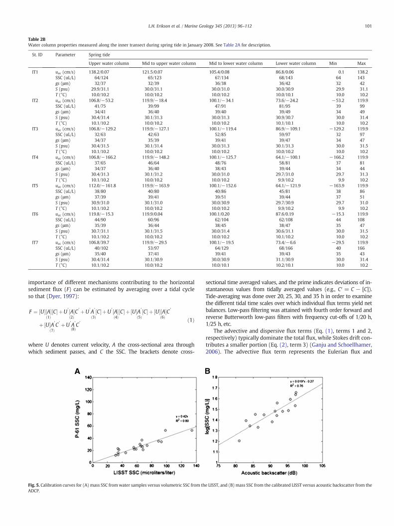
Table 2BWater column properties measured along the inner transect during spring tide in January 2008. See Table 2A for description.

St. ID Parameter Spring tide

Upper water column Mid to upper water column Mid to lower water column Lower water column Min Max

IT1 uac (cm/s) 138.2/0.07 121.5/0.07 105.4/0.08 86.8/0.06 0.1 138.2SSC (uL/L) 64/124 65/123 67/134 68/143 64 143gs (μm) 32/37 32/39 36/38 36/42 32 42S (psu) 29.9/31.1 30.0/31.1 30.0/31.0 30.0/30.9 29.9 31.1T (°C) 10.0/10.2 10.0/10.2 10.0/10.2 10.0/10.1 10.0 10.2

IT2 uac (cm/s) 106.8/−53.2 119.9/−18.4 100.1/−34.1 73.6/−24.2 −53.2 119.9SSC (uL/L) 41/75 39/99 47/91 81/95 39 99gs (μm) 34/41 36/40 39/40 39/49 34 49S (psu) 30.4/31.4 30.1/31.3 30.0/31.3 30.9/30.7 30.0 31.4T (°C) 10.1/10.2 10.0/10.2 10.0/10.2 10.1/10.1 10.0 10.2

IT3 uac (cm/s) 106.8/−129.2 119.9/−127.1 100.1/−119.4 86.9/−109.1 −129.2 119.9SSC (uL/L) 32/63 42/63 52/85 59/97 32 97gs (μm) 34/37 35/39 39/41 39/47 34 47S (psu) 30.4/31.5 30.1/31.4 30.0/31.3 30.1/31.3 30.0 31.5T (°C) 10.1/10.2 10.0/10.2 10.0/10.2 10.0/10.2 10.0 10.2

IT4 uac (cm/s) 106.8/−166.2 119.9/−148.2 100.1/−125.7 64.1/−100.1 −166.2 119.9SSC (uL/L) 37/65 46/64 48/76 58/81 37 81gs (μm) 34/37 36/40 38/43 39/44 34 44S (psu) 30.4/31.3 30.1/31.2 30.0/31.0 29.7/31.0 29.7 31.3T (°C) 10.1/10.2 10.0/10.2 10.0/10.2 9.9/10.2 9.9 10.2

IT5 uac (cm/s) 112.0/−161.8 119.9/−163.9 100.1/−152.6 64.1/−121.9 −163.9 119.9SSC (uL/L) 38/80 40/80 40/86 45/81 38 86gs (μm) 37/39 39/41 39/51 39/44 37 51S (psu) 30.9/31.0 30.1/31.0 30.0/30.9 29.7/30.9 29.7 31.0T (°C) 10.1/10.2 10.0/10.2 10.0/10.2 9.9/10.2 9.9 10.2

IT6 uac (cm/s) 119.8/−15.3 119.9/0.04 100.1/0.20 87.6/0.19 −15.3 119.9SSC (uL/L) 44/90 60/96 62/104 62/108 44 108gs (μm) 35/39 36/44 38/45 38/47 35 47S (psu) 30.7/31.1 30.1/31.5 30.0/31.4 30.6/31.1 30.0 31.5T (°C) 10.1/10.2 10.0/10.2 10.0/10.2 10.1/10.2 10.0 10.2

IT7 uac (cm/s) 106.8/39.7 119.9/−29.5 100.1/−19.5 73.4/−6.6 −29.5 119.9SSC (uL/L) 40/102 53/97 64/129 68/166 40 166gs (μm) 35/40 37/41 39/41 39/43 35 43S (psu) 30.4/31.4 30.1/30.9 30.0/30.9 31.1/30.9 30.0 31.4T (°C) 10.1/10.2 10.0/10.2 10.0/10.1 10.2/10.1 10.0 10.2

101L.H. Erikson et al. / Marine Geology 345 (2013) 96–112

importance of different mechanisms contributing to the horizontalsediment flux (F) can be estimated by averaging over a tidal cycleso that (Dyer, 1997):

F ¼ U½ � A½ � C½ �1ð Þ

þU′ A½ �C′

2ð ÞþU′A′ C½ �

3ð ÞþU′ A½ � C½ �

4ð Þþ U½ �A′ C½ �

5ð Þþ U½ � A½ �C′

6ð Þ

þ U½ �A′C′

7ð ÞþU′A′C′

8ð Þ

ð1Þ

where U denotes current velocity, A the cross-sectional area throughwhich sediment passes, and C the SSC. The brackets denote cross-

Fig. 5. Calibration curves for (A) mass SSC fromwater samples versus volumetric SSC from thADCP.

sectional time averaged values, and the prime indicates deviations of in-stantaneous values from tidally averaged values (e.g., C′ = C − [C]).Tide-averaging was done over 20, 25, 30, and 35 h in order to examinethe different tidal time scales over which individual flux terms yield netbalances. Low-pass filtering was attained with fourth order forward andreverse Butterworth low-pass filters with frequency cut-offs of 1/20 h,1/25 h, etc.

The advective and dispersive flux terms (Eq. (1), terms 1 and 2,respectively) typically dominate the total flux, while Stokes drift con-tributes a smaller portion (Eq. (2), term 3) (Ganju and Schoellhamer,2006). The advective flux term represents the Eulerian flux and

e LISST, and (B) mass SSC from the calibrated LISST versus acoustic backscatter from the

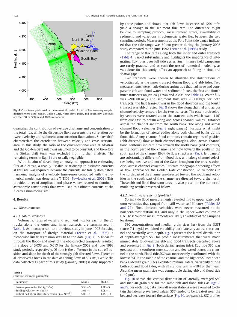
Fig. 6. Curvilinear grids used in the numerical model. A total of five two-way coupleddomains were used: Ocean, Golden Gate, North Bays, Delta, and South Bay. Contoursare the 100 m, 500 m and 1000 m isobaths.

102 L.H. Erikson et al. / Marine Geology 345 (2013) 96–112

quantifies the contribution of average discharge and concentration tothe total flux, while the dispersive flux represents the correlation be-tween velocity and sediment concentration fluctuations. Stokes driftcharacterizes the correlation between velocity and cross-sectionalarea. In this study, the ratio of the cross-sectional area at Alcatrazand the Golden Gate inlet was assumed to be constant, and thereforethe Stokes drift term was excluded from further analysis. Theremaining terms in Eq. (1) are usually negligible.

With the aim of developing an analytical approach to estimatingflux at Alcatraz, a readily useable relationship to estimate currentsat this site was required. Because the currents are tidally dominated,harmonic analysis of a velocity time-series computed with the nu-merical model was done using T_TIDE (Pawlowicz et al., 2002). Thisprovided a set of amplitude and phase values related to dominantastronomic constituents that were used to estimate currents at theAlcatraz monitoring site.

4. Results

4.1. Measurements

4.1.1. Lateral transectsVolumetric rates of water and sediment flux for each of the 25

tracks along the outer and inner transects are summarized inTable 4. As a comparison to a previous study in June 1992 focusingon the transport of dredge material (Teeter et al., 1996), apiece-wise linear regression was fit to the data (Fig. 7). A linear fitthrough the flood- and most of the ebb-directed transports resultedin a slope of 0.033 and 0.013 for the January 2008 and June 1992study periods, respectively. Of note is the difference in the cut-off po-sition and slope for the fit of the strongly ebb directed flows. Teeter etal. observed a break in the data at ebbing flows of 50k m3/s while thedata collected as part of this study (January 2008) is only supported

Table 3Cohesive sediment parameters.

Parameter Mud-2 Mud-4

Erosion parameter (M, kg/m2/s) 5.5E−5 1.3E−5Settling velocity (w, mm/s) 3.0E−1 1.0E−1Critical bed shear stress for erosion (τcre, N/m2) 5.0E−1 1.35E−1

by three points and shows that ebb flows in excess of 120k m3/syield a change in the sediment flux rate. The difference mightbe due to sampling protocol, measurement errors, availability ofsediment, and variations in volumetric water flux between the twosampling periods. Measurements at the Fort Point tide gauge indicat-ed that the tide range was 30 cm greater during the January 2008study compared to the June 1992 Teeter et al. (1996) study.

The range of flux rates along both the inner and outer transects(Table 4) varied substantially and highlights the importance of inte-grating flux rates over full tide cycles. Such intense field campaignsare rarely practical and as such the use of numerical modeling, aswas done for this study, offers an approach to filling in time andspatial gaps.

Two transects were chosen to illustrate the distributions ofvelocities along the inner transect during flood and ebb tides. Twomeasurements were made during spring tide that had large and com-parable ebb and flood water and sediment fluxes, the first and fourthinner transects on Jan 24 (17:44 and 23:05, see Table 4). Water fluxwas ~90,000 m3/s and sediment flux was ~3000 kg/s for bothtransects; the first transect was in the flood direction and the fourthtransect was ebb directed. Fig. 8 shows the along channel and acrosschannel velocity contours for the two transects. The east–north veloc-ity vectors were rotated about the transect axis which was ~140°from due east, to obtain along and across channel values. Distancesacross the channel are from the south bank. The along and acrosschannel flood velocities (Fig. 8 right panels) illustrate what mightbe the formation of lateral eddies along both channel banks duringflood tide. Along-channel flood contours contain regions of positive(ebb directed) flow at both channel margins. Also, across channelflood contours indicate flow toward the north bank (red contours)in the north part of the channel and flow toward the south in thesouth part of the channel. Ebb tide flow structures (Fig. 8, left panels)are substantially different from flood tide, with along channel veloci-ties being positive and out of the Gate throughout the cross section.Also, across channel velocities illustrate topographic steering effectsas flow approaches the Golden Gate constriction, i.e. velocities inthe north part of the channel are directed toward the south and veloc-ities in the south part of the channel are directed toward the north.These ebb and flood flow structures are also present in the numericalmodeling results presented below.

4.1.2. Point measurements (profiles)Spring tide flood measurements revealed mid to upper water col-

umn velocities that ranged from still water to 164 cm/s (Tables 2Aand 2B). Flood directed velocities were never measured at thenorthern-most station, IT1, and only in the upper water column ofIT6. These ‘outlier’measurements are likely an artifact of the samplinglocations.

SSC concentrations and median grain sizes (gs) from the LISST(rmse 7.1 mg/L) exhibited variability both laterally across the chan-nel and vertically with depth. Fig. 9 presents the lateral distributionof depth-averaged SSC for profile measurements that were madeimmediately following the ebb and flood transects described aboveand presented in Fig. 8 (both during spring tide). Ebb tide SSC wasgreatest at the southern-most station and decreased across the chan-nel to the north. Flood tide SSC was more evenly distributed, with thelowest SSC in the middle of the channel and the higher SSC near bothbanks. Median grain sizes exhibited minimal lateral variability duringboth ebb and flood tides, with all stations within ~10% of the mean.Also, the mean grain size was comparable during ebb and flood tide(~40 μm).

Fig. 10 shows the vertical distribution of laterally-averaged SSCand median grain size for the same ebb and flood tides as Figs. 8and 9. For each tide, data from all seven stations were averaged to ob-tain the laterally-averaged values. SSC tended to be greatest near thebed and decrease toward the surface (Fig. 10, top panels). SSC profiles

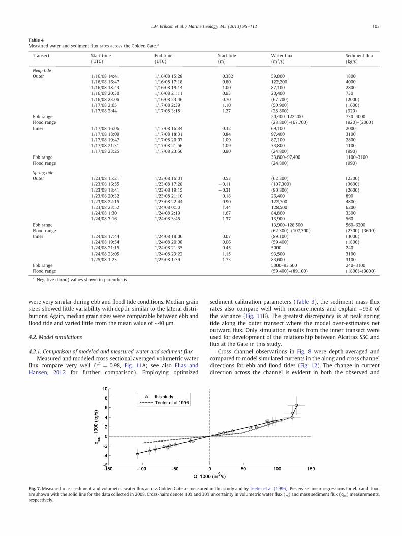
Table 4Measured water and sediment flux rates across the Golden Gate.a

Transect Start time End time Start tide Water flux Sediment flux(UTC) (UTC) (m) (m3/s) (kg/s)

Neap tideOuter 1/16/08 14:41 1/16/08 15:28 0.382 59,800 1800

1/16/08 16:47 1/16/08 17:18 0.80 122,200 40001/16/08 18:43 1/16/08 19:14 1.00 87,100 28001/16/08 20:30 1/16/08 21:11 0.93 20,400 7301/16/08 23:06 1/16/08 23:46 0.70 (67,700) (2000)1/17/08 2:05 1/17/08 2:39 1.10 (50,900) (1600)1/17/08 2:44 1/17/08 3:18 1.27 (28,800) (920)

Ebb range 20,400–122,200 730–4000Flood range (28,800)–(67,700) (920)–(2000)Inner 1/17/08 16:06 1/17/08 16:34 0.32 69,100 2000

1/17/08 18:09 1/17/08 18:31 0.84 97,400 31001/17/08 19:47 1/17/08 20:07 1.09 87,100 28001/17/08 21:31 1/17/08 21:56 1.09 33,800 11001/17/08 23:25 1/17/08 23:50 0.90 (24,800) (990)

Ebb range 33,800–97,400 1100–3100Flood range (24,800) (990)

Spring tideOuter 1/23/08 15:21 1/23/08 16:01 0.53 (62,300) (2300)

1/23/08 16:55 1/23/08 17:28 −0.11 (107,300) (3600)1/23/08 18:41 1/23/08 19:15 −0.31 (80,800) (2600)1/23/08 20:32 1/23/08 21:10 0.18 26,400 8901/23/08 22:15 1/23/08 22:44 0.90 122,700 48001/23/08 23:52 1/24/08 0:50 1.44 128,500 62001/24/08 1:30 1/24/08 2:19 1.67 84,800 33001/24/08 3:16 1/24/08 3:45 1.37 13,900 560

Ebb range 13,900–128,500 560–6200Flood range (62,300)–(107,300) (2300)–(3600)Inner 1/24/08 17:44 1/24/08 18:06 0.07 (89,100) (3000)

1/24/08 19:54 1/24/08 20:08 0.06 (59,400) (1800)1/24/08 21:15 1/24/08 21:35 0.45 5000 2401/24/08 23:05 1/24/08 23:22 1.15 93,500 31001/25/08 1:23 1/25/08 1:39 1.73 83,600 3100

Ebb range 5000–93,500 240–3100Flood range (59,400)–(89,100) (1800)–(3000)

a Negative (flood) values shown in parenthesis.

103L.H. Erikson et al. / Marine Geology 345 (2013) 96–112

were very similar during ebb and flood tide conditions. Median grainsizes showed little variability with depth, similar to the lateral distri-butions. Again, median grain sizes were comparable between ebb andflood tide and varied little from the mean value of ~40 μm.

4.2. Model simulations

4.2.1. Comparison of modeled and measured water and sediment fluxMeasured andmodeled cross-sectional averaged volumetric water

flux compare very well (r2 = 0.98, Fig. 11A; see also Elias andHansen, 2012 for further comparison). Employing optimized

Fig. 7. Measured mass sediment and volumetric water flux across Golden Gate as measuredare shown with the solid line for the data collected in 2008. Cross-hairs denote 10% and 30%respectively.

sediment calibration parameters (Table 3), the sediment mass fluxrates also compare well with measurements and explain ~93% ofthe variance (Fig. 11B). The greatest discrepancy is at peak springtide along the outer transect where the model over-estimates netoutward flux. Only simulation results from the inner transect wereused for development of the relationship between Alcatraz SSC andflux at the Gate in this study.

Cross channel observations in Fig. 8 were depth-averaged andcompared to model simulated currents in the along and cross channeldirections for ebb and flood tides (Fig. 12). The change in currentdirection across the channel is evident in both the observed and

in this study and by Teeter et al. (1996). Piecewise linear regressions for ebb and flooduncertainty in volumetric water flux (Q) and mass sediment flux (qss) measurements,

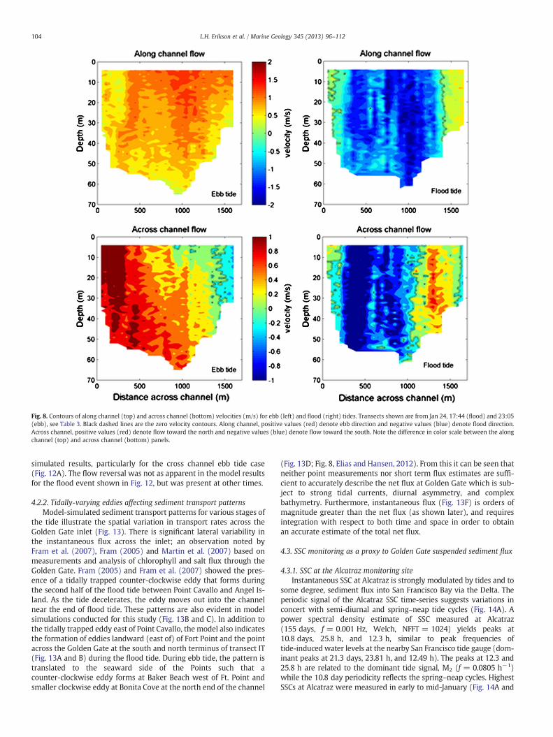
Fig. 8. Contours of along channel (top) and across channel (bottom) velocities (m/s) for ebb (left) and flood (right) tides. Transects shown are from Jan 24, 17:44 (flood) and 23:05(ebb), see Table 3. Black dashed lines are the zero velocity contours. Along channel, positive values (red) denote ebb direction and negative values (blue) denote flood direction.Across channel, positive values (red) denote flow toward the north and negative values (blue) denote flow toward the south. Note the difference in color scale between the alongchannel (top) and across channel (bottom) panels.

104 L.H. Erikson et al. / Marine Geology 345 (2013) 96–112

simulated results, particularly for the cross channel ebb tide case(Fig. 12A). The flow reversal was not as apparent in the model resultsfor the flood event shown in Fig. 12, but was present at other times.

4.2.2. Tidally-varying eddies affecting sediment transport patternsModel-simulated sediment transport patterns for various stages of

the tide illustrate the spatial variation in transport rates across theGolden Gate inlet (Fig. 13). There is significant lateral variability inthe instantaneous flux across the inlet; an observation noted byFram et al. (2007), Fram (2005) and Martin et al. (2007) based onmeasurements and analysis of chlorophyll and salt flux through theGolden Gate. Fram (2005) and Fram et al. (2007) showed the pres-ence of a tidally trapped counter-clockwise eddy that forms duringthe second half of the flood tide between Point Cavallo and Angel Is-land. As the tide decelerates, the eddy moves out into the channelnear the end of flood tide. These patterns are also evident in modelsimulations conducted for this study (Fig. 13B and C). In addition tothe tidally trapped eddy east of Point Cavallo, the model also indicatesthe formation of eddies landward (east of) of Fort Point and the pointacross the Golden Gate at the south and north terminus of transect IT(Fig. 13A and B) during the flood tide. During ebb tide, the pattern istranslated to the seaward side of the Points such that acounter-clockwise eddy forms at Baker Beach west of Ft. Point andsmaller clockwise eddy at Bonita Cove at the north end of the channel

(Fig. 13D; Fig. 8, Elias and Hansen, 2012). From this it can be seen thatneither point measurements nor short term flux estimates are suffi-cient to accurately describe the net flux at Golden Gate which is sub-ject to strong tidal currents, diurnal asymmetry, and complexbathymetry. Furthermore, instantaneous flux (Fig. 13F) is orders ofmagnitude greater than the net flux (as shown later), and requiresintegration with respect to both time and space in order to obtainan accurate estimate of the total net flux.

4.3. SSC monitoring as a proxy to Golden Gate suspended sediment flux

4.3.1. SSC at the Alcatraz monitoring siteInstantaneous SSC at Alcatraz is strongly modulated by tides and to

some degree, sediment flux into San Francisco Bay via the Delta. Theperiodic signal of the Alcatraz SSC time-series suggests variations inconcert with semi-diurnal and spring–neap tide cycles (Fig. 14A). Apower spectral density estimate of SSC measured at Alcatraz(155 days, f = 0.001 Hz, Welch, NFFT = 1024) yields peaks at10.8 days, 25.8 h, and 12.3 h, similar to peak frequencies oftide-induced water levels at the nearby San Francisco tide gauge (dom-inant peaks at 21.3 days, 23.81 h, and 12.49 h). The peaks at 12.3 and25.8 h are related to the dominant tide signal, M2 (f = 0.0805 h−1)while the 10.8 day periodicity reflects the spring–neap cycles. HighestSSCs at Alcatraz were measured in early to mid-January (Fig. 14A and

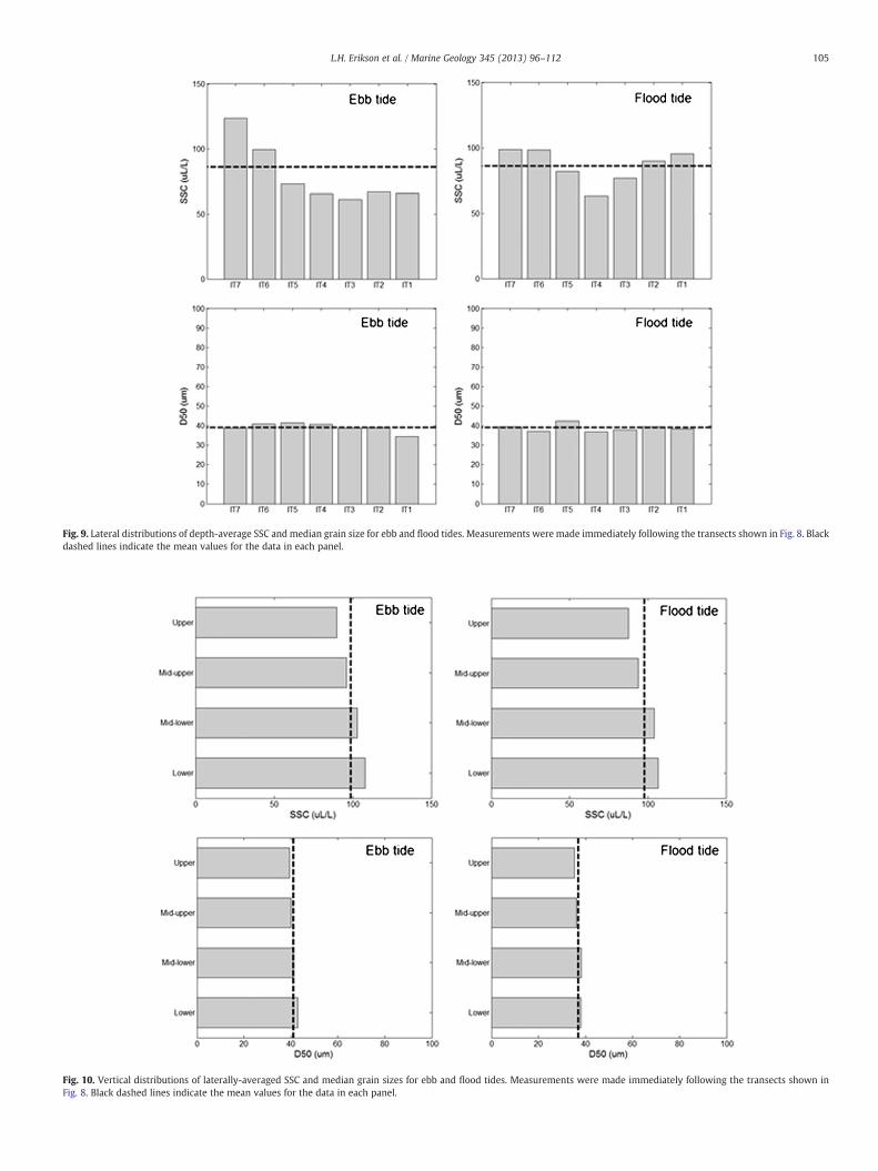
Fig. 9. Lateral distributions of depth-average SSC andmedian grain size for ebb and flood tides. Measurements were made immediately following the transects shown in Fig. 8. Blackdashed lines indicate the mean values for the data in each panel.

Fig. 10. Vertical distributions of laterally-averaged SSC and median grain sizes for ebb and flood tides. Measurements were made immediately following the transects shown inFig. 8. Black dashed lines indicate the mean values for the data in each panel.

105L.H. Erikson et al. / Marine Geology 345 (2013) 96–112

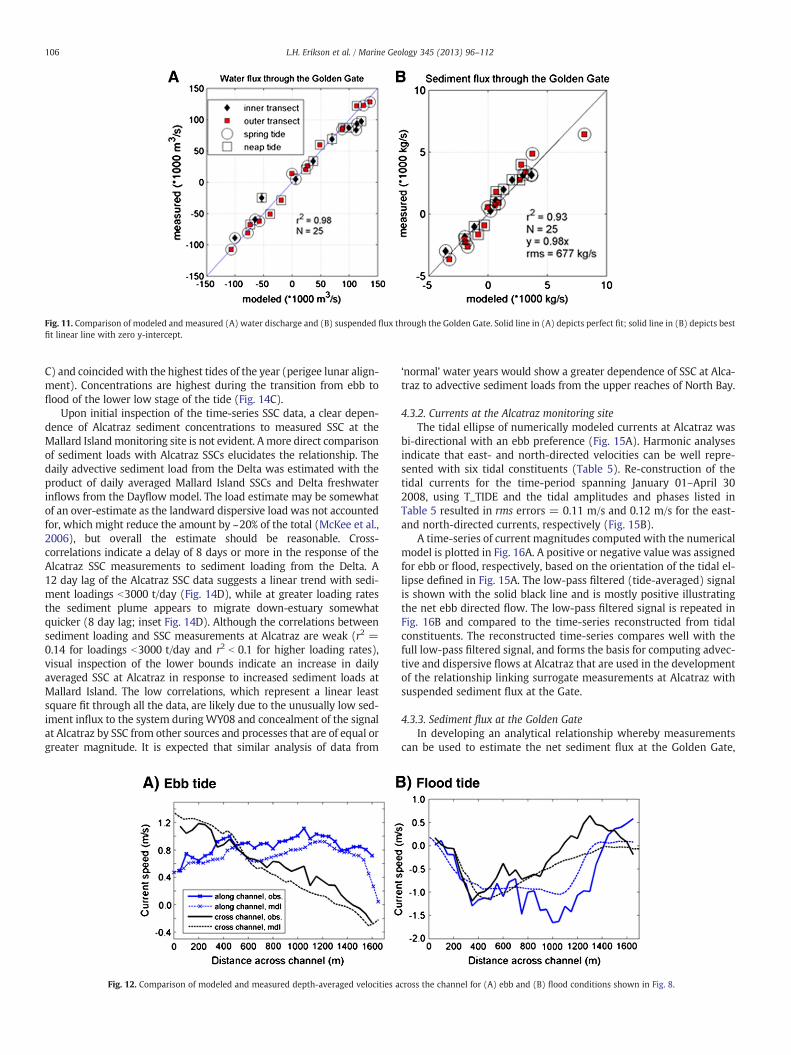
Fig. 11. Comparison of modeled and measured (A) water discharge and (B) suspended flux through the Golden Gate. Solid line in (A) depicts perfect fit; solid line in (B) depicts bestfit linear line with zero y-intercept.

106 L.H. Erikson et al. / Marine Geology 345 (2013) 96–112

C) and coincidedwith the highest tides of the year (perigee lunar align-ment). Concentrations are highest during the transition from ebb toflood of the lower low stage of the tide (Fig. 14C).

Upon initial inspection of the time-series SSC data, a clear depen-dence of Alcatraz sediment concentrations to measured SSC at theMallard Islandmonitoring site is not evident. Amore direct comparisonof sediment loads with Alcatraz SSCs elucidates the relationship. Thedaily advective sediment load from the Delta was estimated with theproduct of daily averaged Mallard Island SSCs and Delta freshwaterinflows from the Dayflow model. The load estimate may be somewhatof an over-estimate as the landward dispersive load was not accountedfor, which might reduce the amount by ~20% of the total (McKee et al.,2006), but overall the estimate should be reasonable. Cross-correlations indicate a delay of 8 days or more in the response of theAlcatraz SSC measurements to sediment loading from the Delta. A12 day lag of the Alcatraz SSC data suggests a linear trend with sedi-ment loadings b3000 t/day (Fig. 14D), while at greater loading ratesthe sediment plume appears to migrate down-estuary somewhatquicker (8 day lag; inset Fig. 14D). Although the correlations betweensediment loading and SSC measurements at Alcatraz are weak (r2 =0.14 for loadings b3000 t/day and r2 b 0.1 for higher loading rates),visual inspection of the lower bounds indicate an increase in dailyaveraged SSC at Alcatraz in response to increased sediment loads atMallard Island. The low correlations, which represent a linear leastsquare fit through all the data, are likely due to the unusually low sed-iment influx to the system duringWY08 and concealment of the signalat Alcatraz by SSC from other sources and processes that are of equal orgreater magnitude. It is expected that similar analysis of data from

Fig. 12. Comparison of modeled and measured depth-averaged velocities a

‘normal’ water years would show a greater dependence of SSC at Alca-traz to advective sediment loads from the upper reaches of North Bay.

4.3.2. Currents at the Alcatraz monitoring siteThe tidal ellipse of numerically modeled currents at Alcatraz was

bi-directional with an ebb preference (Fig. 15A). Harmonic analysesindicate that east- and north-directed velocities can be well repre-sented with six tidal constituents (Table 5). Re-construction of thetidal currents for the time-period spanning January 01–April 302008, using T_TIDE and the tidal amplitudes and phases listed inTable 5 resulted in rms errors = 0.11 m/s and 0.12 m/s for the east-and north-directed currents, respectively (Fig. 15B).

A time-series of current magnitudes computed with the numericalmodel is plotted in Fig. 16A. A positive or negative value was assignedfor ebb or flood, respectively, based on the orientation of the tidal el-lipse defined in Fig. 15A. The low-pass filtered (tide-averaged) signalis shown with the solid black line and is mostly positive illustratingthe net ebb directed flow. The low-pass filtered signal is repeated inFig. 16B and compared to the time-series reconstructed from tidalconstituents. The reconstructed time-series compares well with thefull low-pass filtered signal, and forms the basis for computing advec-tive and dispersive flows at Alcatraz that are used in the developmentof the relationship linking surrogate measurements at Alcatraz withsuspended sediment flux at the Gate.

4.3.3. Sediment flux at the Golden GateIn developing an analytical relationship whereby measurements

can be used to estimate the net sediment flux at the Golden Gate,

cross the channel for (A) ebb and (B) flood conditions shown in Fig. 8.

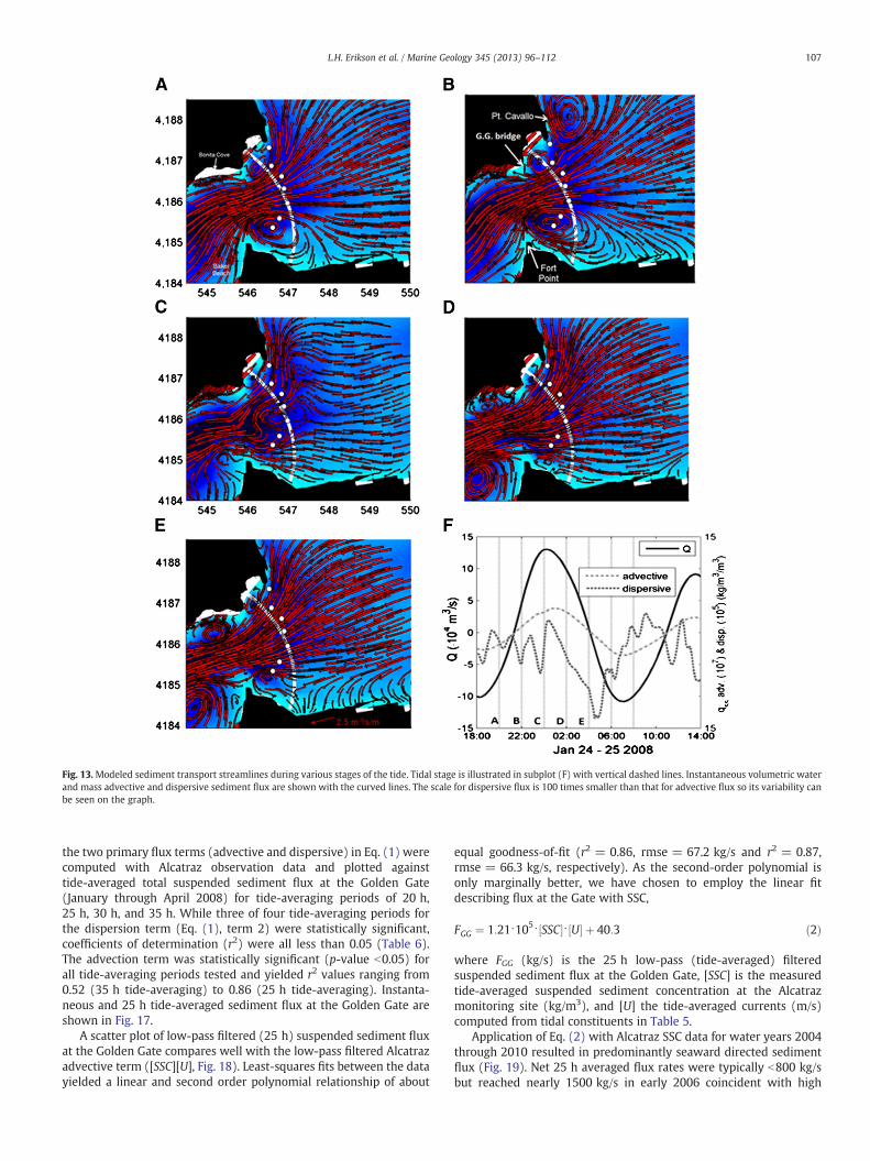
Fig. 13.Modeled sediment transport streamlines during various stages of the tide. Tidal stage is illustrated in subplot (F) with vertical dashed lines. Instantaneous volumetric waterand mass advective and dispersive sediment flux are shown with the curved lines. The scale for dispersive flux is 100 times smaller than that for advective flux so its variability canbe seen on the graph.

107L.H. Erikson et al. / Marine Geology 345 (2013) 96–112

the two primary flux terms (advective and dispersive) in Eq. (1) werecomputed with Alcatraz observation data and plotted againsttide-averaged total suspended sediment flux at the Golden Gate(January through April 2008) for tide-averaging periods of 20 h,25 h, 30 h, and 35 h. While three of four tide-averaging periods forthe dispersion term (Eq. (1), term 2) were statistically significant,coefficients of determination (r2) were all less than 0.05 (Table 6).The advection term was statistically significant (p-value b0.05) forall tide-averaging periods tested and yielded r2 values ranging from0.52 (35 h tide-averaging) to 0.86 (25 h tide-averaging). Instanta-neous and 25 h tide-averaged sediment flux at the Golden Gate areshown in Fig. 17.

A scatter plot of low-pass filtered (25 h) suspended sediment fluxat the Golden Gate compares well with the low-pass filtered Alcatrazadvective term ([SSC][U], Fig. 18). Least-squares fits between the datayielded a linear and second order polynomial relationship of about

equal goodness-of-fit (r2 = 0.86, rmse = 67.2 kg/s and r2 = 0.87,rmse = 66.3 kg/s, respectively). As the second-order polynomial isonly marginally better, we have chosen to employ the linear fitdescribing flux at the Gate with SSC,

FGG ¼ 1:21⋅105⋅ SSC½ �⋅ U½ � þ 40:3 ð2Þ

where FGG (kg/s) is the 25 h low-pass (tide-averaged) filteredsuspended sediment flux at the Golden Gate, [SSC] is the measuredtide-averaged suspended sediment concentration at the Alcatrazmonitoring site (kg/m3), and [U] the tide-averaged currents (m/s)computed from tidal constituents in Table 5.

Application of Eq. (2) with Alcatraz SSC data for water years 2004through 2010 resulted in predominantly seaward directed sedimentflux (Fig. 19). Net 25 h averaged flux rates were typically b800 kg/sbut reached nearly 1500 kg/s in early 2006 coincident with high

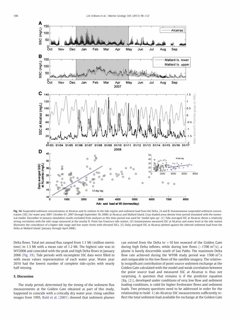
Fig. 14. Suspended sediment concentrations at Alcatraz and its relation to the tide regime and sediment load from the Delta. (A and B) Instantaneous suspended sediment concen-tration (SSC) for water year 2007 (October 01, 2007 through September 30, 2008) at Alcatraz and Mallard Island. Gray shaded areas denote time-period simulated with the numer-ical model. December to January simulation results excluded from analyses as this time-period was used for ‘model spin-up’. (C) Tide-averaged SSC at Alcatraz shows a relativelystrong correlation with the tide-range measured at the nearby Ft. Point San Francisco tide station. (D) Instantaneous measured SSC at Alcatraz and water level at the tide stationillustrates the coincidence of a higher tide range and low water levels with elevated SSCs. (E) Daily averaged SSC at Alcatraz plotted against the inferred sediment load from theDelta at Mallard Island (January through April 2008).

108 L.H. Erikson et al. / Marine Geology 345 (2013) 96–112

Delta flows. Total net annual flux ranged from 1.1 Mt (million metrictons) to 1.3 Mt with a mean rate of 1.2 Mt. The highest rate was inWY2006 and coincided with the peak and high Delta flows in January2006 (Fig. 19). Tide periods with incomplete SSC data were filled inwith mean values representative of each water year. Water year2010 had the lowest number of complete tide-cycles with nearlyhalf missing.

5. Discussion

The study period, determined by the timing of the sediment fluxmeasurements at the Golden Gate obtained as part of this study,happened to coincide with a critically dry water year. Using satelliteimages from 1995, Ruhl et al. (2001) showed that sediment plumes

can extend from the Delta to >10 km seaward of the Golden Gateduring high Delta inflows, while during low flows (~1700 m3/s), aplume is barely discernible south of San Pablo. The maximum Deltaflow rate achieved during the WY08 study period was 1500 m3/sand comparable to the low flows of the satellite imagery. The relative-ly insignificant contribution of point source sediment exchange at theGolden Gate calculated with the model and weak correlation betweenthe point source load and measured SSC at Alcatraz is thus notsurprising. A question that remains is if the predictor equation(Eq. (2)), developed under conditions of very low flow and sedimentloading conditions, is valid for higher freshwater flows and sedimentloads. Two primary questions need to be addressed in order for therelationship to hold: 1) do Alcatraz SSC measurements sufficiently re-flect the total sediment load available for exchange at the Golden Gate

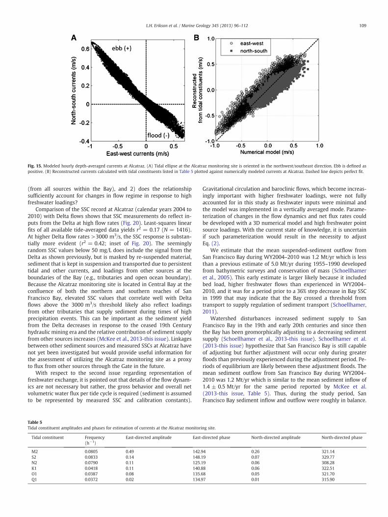
Fig. 15. Modeled hourly depth-averaged currents at Alcatraz. (A) Tidal ellipse at the Alcatraz monitoring site is oriented in the northwest/southeast direction. Ebb is defined aspositive. (B) Reconstructed currents calculated with tidal constituents listed in Table 5 plotted against numerically modeled currents at Alcatraz. Dashed line depicts perfect fit.

109L.H. Erikson et al. / Marine Geology 345 (2013) 96–112

(from all sources within the Bay), and 2) does the relationshipsufficiently account for changes in flow regime in response to highfreshwater loadings?

Comparison of the SSC record at Alcatraz (calendar years 2004 to2010) with Delta flows shows that SSC measurements do reflect in-puts from the Delta at high flow rates (Fig. 20). Least-squares linearfits of all available tide-averaged data yields r2 = 0.17 (N = 1416).At higher Delta flow rates >3000 m3/s, the SSC response is substan-tially more evident (r2 = 0.42; inset of Fig. 20). The seeminglyrandom SSC values below 50 mg/L does include the signal from theDelta as shown previously, but is masked by re-suspended material,sediment that is kept in suspension and transported due to persistenttidal and other currents, and loadings from other sources at theboundaries of the Bay (e.g., tributaries and open ocean boundary).Because the Alcatraz monitoring site is located in Central Bay at theconfluence of both the northern and southern reaches of SanFrancisco Bay, elevated SSC values that correlate well with Deltaflows above the 3000 m3/s threshold likely also reflect loadingsfrom other tributaries that supply sediment during times of highprecipitation events. This can be important as the sediment yieldfrom the Delta decreases in response to the ceased 19th Centuryhydraulic mining era and the relative contribution of sediment supplyfrom other sources increases (McKee et al., 2013-this issue). Linkagesbetween other sediment sources and measured SSCs at Alcatraz havenot yet been investigated but would provide useful information forthe assessment of utilizing the Alcatraz monitoring site as a proxyto flux from other sources through the Gate in the future.

With respect to the second issue regarding representation offreshwater exchange, it is pointed out that details of the flow dynam-ics are not necessary but rather, the gross behavior and overall netvolumetric water flux per tide cycle is required (sediment is assumedto be represented by measured SSC and calibration constants).

Table 5Tidal constituent amplitudes and phases for estimation of currents at the Alcatraz monitori

Tidal constituent Frequency East-directed amplitude East-(h−1)

M2 0.0805 0.49 142.9S2 0.0833 0.14 148.1N2 0.0790 0.11 125.1K1 0.0418 0.11 140.8O1 0.0387 0.08 135.6Q1 0.0372 0.02 134.9

Gravitational circulation and baroclinic flows, which become increas-ingly important with higher freshwater loadings, were not fullyaccounted for in this study as freshwater inputs were minimal andthe model was implemented in a vertically averaged mode. Parame-terization of changes in the flow dynamics and net flux rates couldbe developed with a 3D numerical model and high freshwater pointsource loadings. With the current state of knowledge, it is uncertainif such parameterization would result in the necessity to adjustEq. (2).

We estimate that the mean suspended-sediment outflow fromSan Francisco Bay during WY2004–2010 was 1.2 Mt/yr which is lessthan a previous estimate of 5.0 Mt/yr during 1955–1990 developedfrom bathymetric surveys and conservation of mass (Schoellhameret al., 2005). This early estimate is larger likely because it includedbed load, higher freshwater flows than experienced in WY2004–2010, and it was for a period prior to a 36% step decrease in Bay SSCin 1999 that may indicate that the Bay crossed a threshold fromtransport to supply regulation of sediment transport (Schoellhamer,2011).

Watershed disturbances increased sediment supply to SanFrancisco Bay in the 19th and early 20th centuries and since thenthe Bay has been geomorphically adjusting to a decreasing sedimentsupply (Schoellhamer et al., 2013-this issue). Schoellhamer et al.(2013-this issue) hypothesize that San Francisco Bay is still capableof adjusting but further adjustment will occur only during greaterfloods than previously experienced during the adjustment period. Pe-riods of equilibrium are likely between these adjustment floods. Themean sediment outflow from San Francisco Bay during WY2004–2010 was 1.2 Mt/yr which is similar to the mean sediment inflow of1.4 ± 0.5 Mt/yr for the same period reported by McKee et al.(2013-this issue, Table 5). Thus, during the study period, SanFrancisco Bay sediment inflow and outflow were roughly in balance.

ng site.

directed phase North-directed amplitude North-directed phase

4 0.26 321.149 0.07 329.779 0.06 308.288 0.06 322.518 0.05 321.707 0.01 315.90

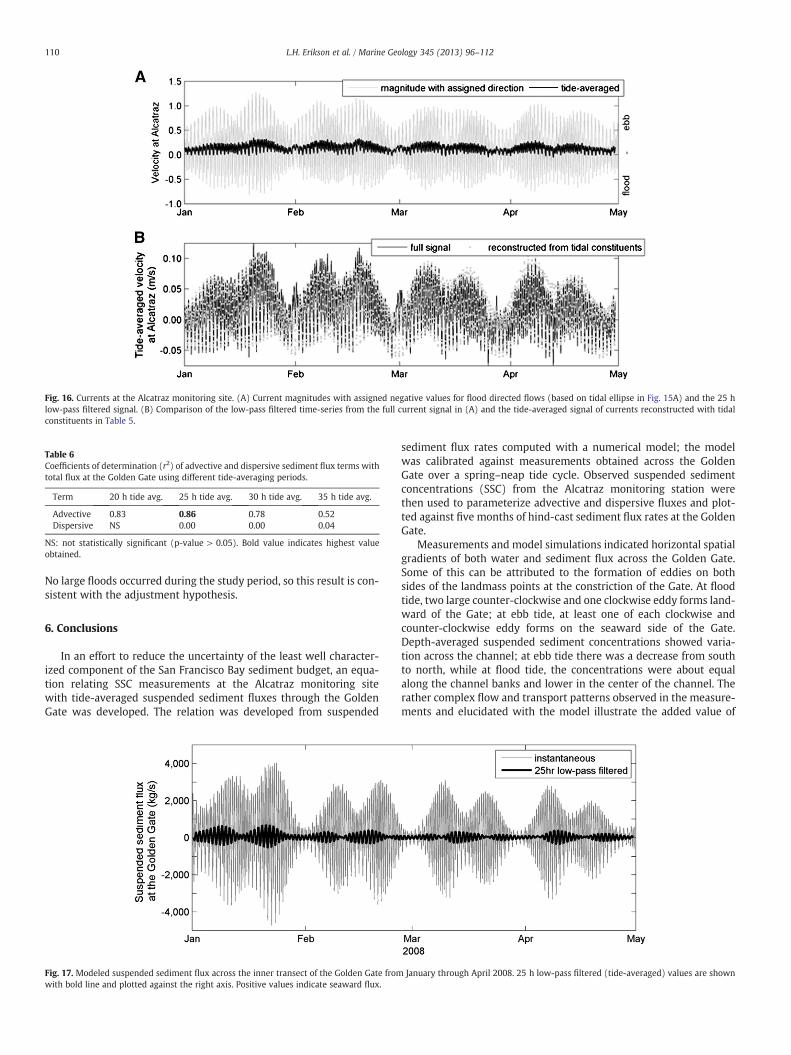
Fig. 16. Currents at the Alcatraz monitoring site. (A) Current magnitudes with assigned negative values for flood directed flows (based on tidal ellipse in Fig. 15A) and the 25 hlow-pass filtered signal. (B) Comparison of the low-pass filtered time-series from the full current signal in (A) and the tide-averaged signal of currents reconstructed with tidalconstituents in Table 5.

Table 6Coefficients of determination (r2) of advective and dispersive sediment flux terms withtotal flux at the Golden Gate using different tide-averaging periods.

Term 20 h tide avg. 25 h tide avg. 30 h tide avg. 35 h tide avg.

Advective 0.83 0.86 0.78 0.52Dispersive NS 0.00 0.00 0.04

NS: not statistically significant (p-value > 0.05). Bold value indicates highest valueobtained.

110 L.H. Erikson et al. / Marine Geology 345 (2013) 96–112

No large floods occurred during the study period, so this result is con-sistent with the adjustment hypothesis.

6. Conclusions

In an effort to reduce the uncertainty of the least well character-ized component of the San Francisco Bay sediment budget, an equa-tion relating SSC measurements at the Alcatraz monitoring sitewith tide-averaged suspended sediment fluxes through the GoldenGate was developed. The relation was developed from suspended

Fig. 17. Modeled suspended sediment flux across the inner transect of the Golden Gate fromwith bold line and plotted against the right axis. Positive values indicate seaward flux.

sediment flux rates computed with a numerical model; the modelwas calibrated against measurements obtained across the GoldenGate over a spring–neap tide cycle. Observed suspended sedimentconcentrations (SSC) from the Alcatraz monitoring station werethen used to parameterize advective and dispersive fluxes and plot-ted against five months of hind-cast sediment flux rates at the GoldenGate.

Measurements and model simulations indicated horizontal spatialgradients of both water and sediment flux across the Golden Gate.Some of this can be attributed to the formation of eddies on bothsides of the landmass points at the constriction of the Gate. At floodtide, two large counter-clockwise and one clockwise eddy forms land-ward of the Gate; at ebb tide, at least one of each clockwise andcounter-clockwise eddy forms on the seaward side of the Gate.Depth-averaged suspended sediment concentrations showed varia-tion across the channel; at ebb tide there was a decrease from southto north, while at flood tide, the concentrations were about equalalong the channel banks and lower in the center of the channel. Therather complex flow and transport patterns observed in the measure-ments and elucidated with the model illustrate the added value of

January through April 2008. 25 h low-pass filtered (tide-averaged) values are shown

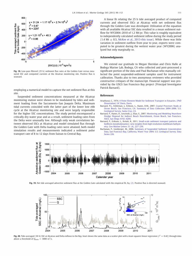
Fig. 18. Low-pass filtered (25 h) sediment flux rates at the Golden Gate versus mea-sured SSC and computed currents at the Alcatraz monitoring site. Positive flux isseaward.

111L.H. Erikson et al. / Marine Geology 345 (2013) 96–112

employing a numerical model to capture the net sediment flux at thissite.

Suspended sediment concentrations measured at the Alcatrazmonitoring station were shown to be modulated by tides and sedi-ment loading from the Sacramento–San Joaquin Delta. Maximumtidal currents coincided with the latter part of the lower low ebbcycle at the Alcatraz monitoring site and were largely responsiblefor the higher SSC concentrations. The study period encompassed acritically dry water year and as a result, sediment loading rates fromthe Delta were unusually low. Although only weak correlations be-tween observed SSCs at Alcatraz and model simulated flux throughthe Golden Gate with Delta loading rates were attained, both modelsimulation results and measurements indicated a sediment pulsetransport rate of 8 to 12 days from Suisun to Central Bay.

Fig. 19. Net tide averaged advective sediment flux at the Golden Gate calcu

Fig. 20. Tide-averaged (30 h) SSC at Alcatraz and Delta inflows to the Bay. Inset shows the saabove a threshold of QDelta = 3000 m3/s.

A linear fit relating the 25 h tide averaged product of computedcurrents and observed SSCs at Alcatraz with net sediment fluxthrough the Golden Gate was developed. Utilization of the equationwith all available Alcatraz SSC data resulted in a mean sediment out-flow for WY2004–2010 of 1.2 Mt/yr. This value is roughly equivalentto independently calculated sediment inflow during the study period(1.4 Mt ± 0.5, McKee et al., 2013-this issue). While there was littlevariation in sediment outflow from year to year, exports were com-puted to be greatest during the wettest water year (WY2006) ana-lyzed but only marginally so.

Acknowledgments

We extend our gratitude to Megan Sheridan and Chris Halle atBodega Marine Lab, Bodega, CA who collected and post-processed asignificant portion of the data and Paul Buchanan who manually col-lected the point suspended-sediment samples used for instrumentcalibration. Thanks also to two anonymous reviewers who providedconstructive critiques of the manuscript. Financial support was pro-vided by the USGS San Francisco Bay project (Principal InvestigatorPatrick Barnard).

References

Ariathurai, C., 1974. A Finite Element Model for Sediment Transport in Estuaries. (PhDDissertation) UC Davis, Davis.

Barnard, P.L., Eshleman, J., Erikson, L., Hanes, D.M., 2007. Coastal Processes Study atOcean Beach, San Francisco, CA: Summary of Data Collection 2004–2006. U.S.Geological Survey, Santa Cruz, CA.

Barnard, P., Hanes, D., Lescinski, J., Elias, E., 2007. Monitoring and Modeling NearshoreDredge Disposal for Indirect Beach Nourishment, Ocean Beach, San Francisco.ASCE, San Diego 4192–4204.

Barnard, P., Erikson, L., Kvitek, R., 2011. Small-scale sediment transport patterns andbedform morphodynamics: new insights from high resolution multibeam bathym-etry. Geo-Marine Letters 31 (4), 227–236.

Buchanan, P., Lionberger, M., 2006. Summary of Suspended Sediment ConcentrationData, San Francisco Bay, California, Water Year 2004. U.S. Geological Survey. DataSeries 226.

lated with the empirical fit, Eq. (2). Positive flux is directed seaward.

me data as a scatter plot with a least-squares linear regression (r2 = 0.42) through data

112 L.H. Erikson et al. / Marine Geology 345 (2013) 96–112

Carlson, P., McCulloch, D., 1974. Aerial Observations of Suspended Sediment Plumes inSan Francisco Bay and Adjacent Pacific Ocean. U.S. Geological Survey, s.l.

CDWR, 2012. DAYFLOW program documentation and DAYFLOW data summary user'sguide. Available at: http://iep.water.ca.gov/dayflow (Accessed 2012).

Cheng, R., Smith, R., 1998. A Nowcast Model for Tides and Tidal Currents in SanFrancisco Bay, California. Marine Technology Society, Baltimore, MD 537–543.

Chin, J., et al., 2010. Estuarine Sedimentation, Sediment Character, and ForaminiferalDistribution in Central San Francisco Bay, California. U.S. Geological Survey, s.l.

Chin, J.L., Wong, F.L., Carlson, P.R., 2004. Shifting shoals and shattered rocks— howmanhas transformed the floor of west-central San Francisco Bay. U.S. Geological SurveyCircular 1259.

Conomos, T., 1979. Properties and Circulation of San Francisco Bay Water. Pacific Divi-sion of the American Association for the Advancement of Science, San Francisco47–84.

Conomos, T., Peterson, D., 1977. Suspended-particle transport and circulation inSan Francisco Bay, an overview. Estuarine Processes. Academic Press, NewYork, pp. 82–97.

Conomos, T., Smith, R., Gartner, J., 1985. Environmental setting of San Francisco Bay.Hydrobiologia 129 (1), 1–12.

Deltares, 2011. User Manual Delft3D-FLOW. 3.15.18392.Dyer, K., 1997. Estuaries — Physical Introduction, 2nd ed. John Wiley and Sons,

Chichester.Edwards, T.K., Glysson, G.D., 1999. Field methods for measurements of fluvial sedi-

ments. U.S. Geological Survey, Techniques of Water Resources Investigations,Book3, Chapter C2.

Egbert, G., Erofeeva, S., 2002. Efficient inverse modeling of barotropic ocean tides.Journal of Atmospheric and Oceanic Technology 183–204.

Egbert, G., Bennet, A., Foreman, M., 1994. TOPEX/POSEIDON tides estimated using aglobal inverse model. Journal of Geophysical Research 99 (C12), 821–824.

Elias, E.P.L., Hansen, J.E., 2012. Understanding processes controlling sediment trans-ports at the mouth of a highly energetic inlet system (San Francisco Bay, CA).Marine Geology. http://dx.doi.org/10.1016/j.margeo.2012.07.003.

Fram, J.P., 2005. Exchange at the estuary-ocean interface: Fluxes through the goldengate channel. Ph.D. dissertation, University of California, Berkeley.

Fram, J., Martin, M., Stacey, M., 2007. Dispersive fluxes between the coastal ocean andsemi-enclosed estuarine basin. Physical Oceanography 1645–1660.

Ganju, N., Schoellhamer, D., 2006. Annual sediment flux estimates in a tidal strait usingsurrogate measurements. Estuarine, Coastal and Shelf Science 69, 165–178.

Ganju, N., Schoellhamer, D., 2009. Calibration of an estuarine sediment transport modelto sediment fluxes as an intermediate step for simulation of geomorphic evolution.Continental Shelf Research 29, 148–158.

Gartner, J.W., 2004. Estimating suspended solids concentrations from backscatter in-tensity measured by acoustic Doppler current profiler in San Francisco Bay, Califor-nia. Marine Geology 211, 169–187.

Hauck, L., Teeter, A., Pankow, W., Evans, R.J., 1990. San Francisco Bay suspended sedi-ment movement: report I: summer condition data collection and numericalmodel verification. Technical Report HL-90-6. U.S. Army Engineer Waterways Ex-periment Station, Vicksburg, MS.

Jaffe, B.E., Smith, R., Foxgrover, A., 2007. Anthropogenic influence on sedimentationand intertidal mudflat change in San Pablo Bay, California: 1856–1983. Estuarine,Coastal and Shelf Science 73, 175–187.

Kineke, G., Sternberg, R., 1989. The effect of particle settling velocity on computedsuspended sediment concentration profiles. Marine Geology 90, 159–174.

Krank, K., Milligan, T., 1992. Characteristics of suspended particles at an 11-hour an-chor station in San Francisco Bay, California. Journal of Geophysical Research 97(C7), 11373–11382.

Kroll, G., 1975. Estimate of Sediment Discharges, Santa Ana River at Santa Ana andSanta Maria River at Guadalupe California. U.S. Geological Survey, s.l.

Krone, R., 1962. Flume Studies of the Transport of Sediment in Estuarial ShoalingProcesses. U.C. Berkeley, Berkeley.

Largier, J., 1996. Hydrodynamic exchange between San Francisco Bay and the ocean:the role of ocean circulation and stratification. San Francisco Bay: the ecosystem.AAAS, s.l, pp. 69–104.

Lesser, G.R., Roelvink, J.A., van Kester, J.A.T.M., Stelling, G.S., 2004. Development andvalidation of a three-dimensional morphological model. Coastal Engineering 51(8–9), 883–915.

Locke, J.L., 1971. Sedimentation and Foraminiferal Aspects of the Recent Sediments ofSan Pablo Bay. (M.S. thesis) San Jose State University, San Jose, CA (100 pp.).

Martin, M.A., Fram, J.P., Stacey, M.T., 2007. Seasonal chlorophyll a fluxes between the coast-al Pacific Ocean and San Francisco Bay. Marine Ecology Progress Series 337, 51–61.

McKee, L., Ganju, N., Schoellhamer, D., 2006. Estimates of suspended sediment enteringSan Francisco bay from the Sacramento and San Joaquin Delta, San Francisco Bay,California. Journal of Hydrology 323, 335–352.

McKee, L.J., Lewicki, M., Schoellhamer, D.H., Ganju, N.K., 2013. Comparison of sedimentsupply to San Francisco Bay fromwatersheds draining the Bay Area and the CentralValley of California. Marine Geology 345, 47–62 (this issue).

Mehta, A., 1986. Laboratory studies on cohesive sediment deposition and erosion. In:Dronkers, J., van Leussen, W. (Eds.), Physical Processes in Estuaries. SpringerVerlag, New York.

Monosmith, S., Kimmerer, W., Burau, J., Stacey, M., 2002. Structure and flow-inducedvariability of the subtidal salinity field in Northern San Francisco Bay. Journal ofPhysical Oceanography 32, 3003–3019.

Ogden Beeman and Associates, I., 1992. Sediment Budget for San Francisco Bay: FinalReport. U.S. Army Engineer District, San Francisco.

Parker, D., Norris, D., Nelson, A., 1972. Tidal Exchange at the Golden Gate. ASCE, s.l305–323.

Pawlowicz, R., Beardsley, B., Lentz, S., 2002. Classical tidal harmonic analysis includingerror estimates in MATLAB using T_TIDE. Computers & Geosciences 28, 929–937.

Porterfield, G., 1980. Sediment Transport of Streams Tributary to San Francisco, SanPablo and Suisun Bays, California, 1909–66. U.S. Geological Society, s.l.

Roelvink, J., 2006. Coastal morphodynamic evolution techniques. Coastal Engineering53, 177–187.

Rubin, D.M., McCulloch, D.S., 1979. The movement and equilibrium of bedforms in Cen-tral San Francisco Bay. In: Conomos, T.J. (Ed.), The Urbanized Estuary. American As-sociation for the Advancement of Science, San Francisco Bay, pp. 97–113.

Ruhl, C., Schoellhamer, D., Stumpf, R., Lindsay, C., 2001. Combined use of remote sens-ing and continuous monitoring to analyse the variability of suspended-sedimentconcentrations in San Francisco Bay, California. Estuarine, Coastal and Shelf Science53, 801–812.

Schoellhamer, D.H., 2011. Sudden clearing of estuarine waters upon crossing thethreshold from transport- to supply-regulation of sediment transport as an erod-ible sediment pool is depleted: San Francisco Bay, 1999. Estuaries and Coasts 34,885–899.

Schoellhamer, D.H., Lionberger, M.A., Jaffe, B.E., Ganju, N.K., Wright, S.A., Shellenbarger,G.G., 2005. Bay Sediment Budgets: Sediment Accounting 101: The Pulse of the Es-tuary: Monitoring and Managing Water Quality in the San Francisco Estuary. SanFrancisco Estuary Institute, Oakland, California 58–63 (URL http://www.sfei.org/rmp/pulse/2005/RMP05_PulseoftheEstuary.pdf).

Schoellhamer, D.H., Wright, S.A., Drexler, J.Z., 2013. Adjustment of the San Francisco es-tuary and watershed to decreasing sediment supply in the 20th century. MarineGeology 345, 63–71 (this issue).

Scripps Institution of Oceanography, 2012. The Coastal Data Information Program(CDIP), wave data. http://cdip.ucsd.edu/. Last accessed November 2012.

Simpson, M.R., 2001. Discharge measurements using a broad-band acoustic Dopplercurrent profiler. U.S. Geological Survey, Open-File Report 01-1.

Singer, M.A.R., James, L., 2008. Status of the lower Sacramento Valley flood-control sys-tem within the context of its natural geomorphic setting. Natural Hazards Review9, 104–115.

Smith, L.H., 1987. A review of circulation and mixing studies of San Francisco Bay,California. U.S. Geological Survey Circular, 1015 (38 pp.).

Talke, S., Stacey, M., 2003. The influence of oceanic swell on flows over an estuarineintertidal mudflat in San Francisco Bay. Estuarine, Coastal and Shelf Science 58,541–554.

Teeter, A., 1986. Alcatraz Disposal Site Investigation: Report 3: San Francisco Bay-AlcatrazSite Disposal Erodibility. U.S. Army Engineers Waterway Experiment Station,Vicksburg, MS.

Teeter, A.M., Letter, J.V., Pratt, T.C., Callegan, C.J., Boyt, W.L., 1996. San Francisco Baylong-term management strategy (LTMS) for dredging and disposal. Report 2.Baywide suspended sediment transport modeling. Technical Report #A383413.Army Engineer Waterways Experiment Station, Hydraulics Lab, Vicksburg, MS.

van der Wegen, M., Dastgheib, A., Jaffe, B., Roelvink, D., 2011a. Bed composition gener-ation for morphodynamic modeling: case study of San Pablo Bay in California, USA.Ocean Dynamics 61, 173–186.

van der Wegen, M., Jaffe, B., Roelvink, J., 2011b. Process-based, morphodynamichindcast of decadal. Journal of Geophysical Research 116, 22.

Van Rijn, L., 2007. Unified view of sediment transport by currents and waves. II:suspended transport. Journal of Hydraulic Engineering 133 (6), 668–689.

Wintwerp, J., Van Kesteren, W., 2004. Introduction to the physics of cohesive sedimentin the marine environment. Developments in Sedimentology 56.

Wright, S., Schoellhamer, D., 2004. Trends in the sediment yield of the SacramentoRiver, California, 1957–2001. San Francisco Estuary and Watershed Science 2 (2),14.

Wright, S., Schoellhamer, D., 2005. Estimating sediment budgets at the interface be-tween rivers and estuaries with application to the Sacramento–San Joaquin RiverDelta. Water Resources Research 41.

Zedler, J., Callaway, J., 2001. Tidal wetland functioning. Journal of Coastal ResearchSpecial Issue 2001, 38–64.