the unfinished landscape - quteprints.qut.edu.au/50512/1/stephen_perry_thesis.pdf · nature may...
TRANSCRIPT

The Unfinished LandscapeFractal Geometry and theAesthetics of Ecological Design
ByStephen George PerryGrad. Dip. Land. Arch. Dist. (QUT), MSc. Dist. (London University), BSc. (City University, London)Registered Landscape Architect, AILASchool of DesignQueensland University of Technology
Doctor of Philosophy 2012

This work is dedicated to my wife and partner Robyn Minchinton, without
whose spiritual, intellectual and material support it would not have been
possible.

Keywords
Fractal GeometryLandscape ArchitectureEcological DesignAestheticsNature


Abstract P a g e | i
Abstract
During the late 20th century it was proposed that a design aesthetic reflecting currentecological concerns was required within the overall domain of the built environmentand specifically within landscape design. To address this, some authors suggestedvarious theoretical frameworks upon which such an aesthetic could be based. Withinthese frameworks there was an underlying theme that the patterns and processes ofNature may have the potential to form this aesthetic — an aesthetic based on fractalrather than Euclidean geometry. In order to understand how fractal geometry,described as the geometry of Nature, could become the referent for a design aesthetic,this research examines the mathematical concepts of fractal Geometry, and theunderlying philosophical concepts behind the terms ‘Nature’ and ‘aesthetics’.The findings of this initial research meant that a new definition of Nature was requiredin order to overcome the barrier presented by the western philosophicalNature―culture duality. This new definition of Nature is based on the type and use ofenergy. Similarly, it became clear that current usage of the term aesthetics has more incommon with the term ‘style’ than with its correct philosophical meaning. The aestheticphilosophy of both art and the environment recognises different aesthetic criteriarelated to either the subject or the object, such as: aesthetic experience; aestheticattitude; aesthetic value; aesthetic object; and aesthetic properties. Given these criteria,and the fact that the concept of aesthetics is still an active and ongoing philosophicaldiscussion, this work focuses on the criteria of aesthetic properties and the aestheticexperience or response they engender.The examination of fractal geometry revealed that it is a geometry based on scalerather than on the location of a point within a three-dimensional space. This enablesfractal geometry to describe the complex forms and patterns created through theprocesses of Wild Nature. Although fractal geometry has been used to analyse thepatterns of built environments from a plan perspective, it became clear from the initialreview of the literature that there was a total knowledge vacuum about the fractalproperties of environments experienced every day by people as they move throughthem. To overcome this, 21 different landscapes that ranged from highly developed citycentres to relatively untouched landscapes of Wild Nature have been analysed.
Abstract P a g e | ii
Although this work shows that the fractal dimension can be used to differentiatebetween overall landscape forms, it also shows that by itself it cannot differentiatebetween all images analysed. To overcome this two further parameters based on theunderlying structural geometry embedded within the landscape are discussed. Theseparameters are the Power Spectrum Median Amplitude and the Level of Isotropywithin the Fourier Power Spectrum.Based on the detailed analysis of these parameters a greater understanding of thestructural properties of landscapes has been gained. With this understanding, thisresearch has moved the field of landscape design a step close to being able to articulatea new aesthetic for ecological design.

Papers, Presentations & Joint Research P a g e | iii
Papers, Presentations and Joint Research
Papers and Presentations
Perry S, Reeves R, Sim J. 2008. Landscape design and the language of nature.Landscape Review, 12(2): 3-18.Perry S, Reeves R, Sim J. An old language for a new landscape. AILA NationalConference Shifting Perspectives and Practice, 7-9 May 2009., Melbourne DocklandsPerry S. Landscape Design and the Language of Nature. Live in Queensland Design inthe World Seminar SUPERNATURE: Design Inspired by Nature, 17 September 2009,Queensland University of TechnologyJoint ResearchI have been invited to participate on a landscape preference study being undertaken byProfessor Jack Nasar, Professor of City and Regional Planning, Ohio State University,USA. This study will utilise the landscape fractal analysis techniques developed for thisresearch.

Table of Contents P a g e | iv
Table of Contents
CHAPTER ONE: Scope of Research
Introduction .......................................................................................................1Background to Research .......................................................................................................2Research Rational .......................................................................................................4Overall Research Framework and
Approach .......................................................................................................5Research MethodResearch Limitations .......................................................................................................10Method Limitations, Knowledge Limitations, Personal BiasStructure of Thesis .......................................................................................................12
CHAPTER TWO: Sustainability and Ecological Design
Introduction .......................................................................................................15
Sustainability .......................................................................................................16Environmentalism and PhilosophyDesign and Sustainability .......................................................................................................17Two Approaches to Sustainability, Sustainability and Design PracticeDesign and Culture .......................................................................................................20The Importance of Culture, Design and AdaptationFrameworks for Ecological Design .......................................................................................................22Aesthetics as an Agent of Transformation, Re-connecting Humanity and Nature,The Dynamic Processes and Structural Forms of NatureEcological Design and Landscape
Practice .......................................................................................................24
Conclusion .......................................................................................................25
CHAPTER THREE: The Patterns of Nature
Introduction .......................................................................................................26
Dimensions of Space .......................................................................................................26The Three Dimensions of Euclidean Geometry, The Hausdorff DimensionMonster Curves and Self Similarity .......................................................................................................31The Hilbert Curve, The Koch Curve, The Koch Snowflake, The Sierpinski TriangleThe Mandelbrot Set .......................................................................................................36
Fractal Geometry .......................................................................................................38The Length of a CoastlineFractal Patterning of Nature ...................................................................................................... 41Fractal Dust

Table of Contents P a g e | v
Fractal Patterning of Designed
Forms ...................................................................................................... 45The Golden Ratio, Art and Architecture, Architecture and Picturesque Composition, PatternsLandscapes, Patterns of ArtConclusion ...................................................................................................... 52
CHAPTER FOUR: nature or Nature
Introduction .......................................................................................................54
Nature the Word .......................................................................................................55Pre-Industrial NatureHumanity, Nature and Two
Metaphysical Positions .......................................................................................................58
Ecology and Nature .......................................................................................................61Environmental ProcessesA New Framework for
Understanding Nature .......................................................................................................62Environment and Landscape, Wild Nature, Designed Nature, Designed Environments, NatureConclusion .......................................................................................................68
CHAPTER FIVE: Aesthetics
Introduction .......................................................................................................70
Aesthetics, Ecology and
Environment .......................................................................................................71Cultural Ecology, Visual EcologyBeauty and Aesthetics―A Brief
History .......................................................................................................7218th Century English Aesthetic Development, Beauty and Imagination, Beauty and Sublime,Nature and Design, Bridging the GapThe Picturesque and Beyond .......................................................................................................77The Picturesque as Separate from the Sublime and the BeautifulJC Loudon and the Consequences of
the Gardenesque .......................................................................................................80Landscape design as ArtAesthetics and Nature ...................................................................................................... 84
Environmental Aesthetics ...................................................................................................... 85Cognitive Aesthetics, Non-Cognitive Aesthetics, Aesthetics and ConservationAesthetic as Biological Adaptation ...................................................................................................... 88Biological Laws, Cultural Rules, Personal StrategiesBeauty, Aesthetics and Fractal
Patterning ...................................................................................................... 89

Table of Contents P a g e | vi
A Problematic Aesthetic ...................................................................................................... 90
Conclusion ...................................................................................................... 92
CHAPTER SIX: Measuring the Fractal Dimension of a Landscape
Introduction .......................................................................................................95
The Box Counting Method .......................................................................................................95
The Fractal Dimension of a Digital
Image .......................................................................................................98
Fourier Analysis ...................................................................................................... 98The Fourier Series, The One Dimensional Fourier Transform and the Fractal Dimension ofDigital ImagesFractal Analysis Tools .......................................................................................................105
Conclusion ...................................................................................................... 105
CHAPTER SEVEN: Rating a Landscape
Introduction .......................................................................................................107
The Role of Plants .......................................................................................................108Determining the Ratio of Plants in a LandscapeDetermining the Ratio of Plants in a
Landscape ...................................................................................................... 110Step 1: Initial Visual Inspection, Step 2: Verification, Step 3: Re-evaluationConclusion ...................................................................................................... 112
CHAPTER EIGHT: Fractal Analysis of Landscapes
Introduction .......................................................................................................114Research Question 1 and 2, Research Question 3, Research Question 421 Landscapes .......................................................................................................115
Research Question One ...................................................................................................... 125Fractal Analysis, Data Validity,Research Question Two ...................................................................................................... 129
Research Question Three ...................................................................................................... 131Fractal Dimension as a Measure of Naturalness, Dundowran Beach, London East CentralResearch Question Four ...................................................................................................... 134
Conclusion ...................................................................................................... 135Research Questions 1 & 2, Research Question 3, Research Question 4, The Fractal DimensionBeyond the Fractal Dimension ...................................................................................................... 136Fractal Dimension and Landscape FormOverall Conclusions to Research
Questions ...................................................................................................... 139

Table of Contents P a g e | vii
CHAPTER NINE: Geometric Properties of Landscapes
Introduction .......................................................................................................141
Two-Dimensional Power Spectrum
Analysis .......................................................................................................142Single Spatial Frequency, Orthogonal Spatial Frequencies, Angular Spatial FrequenciesThe Two Dimensional Power
Spectrum of a Landscape Image ...................................................................................................... 146
Two-Dimensional Power Spectra
and Landscape Form ...................................................................................................... 149Vegetation as Power Spectrum Modifier, Curvilinear Form as Power Spectrum ModifierKernel Density Estimation ...................................................................................................... 153Power Spectrum Median AmplitudePower Spectrum Median Amplitude
and Landscape Form ...................................................................................................... 158
Contribution to Knowledge ...................................................................................................... 161
Conclusion ...................................................................................................... 161
Chapter 10: The Unfinished Landscape
Introduction .......................................................................................................163
Towards and Ecological Aesthetic .......................................................................................................165
Appendices
Appendix A: Camera and Software .......................................................................................................169Digital Cameras and Image Quality, Fractal Analysis Code for RAppendix B: Vegetation Rating .......................................................................................................180
Appendix C: Analysis Results ...................................................................................................... 191Landscape Fractal Analysis, Fractal Dimension, Power Spectrum Median Amplitude andVegetation Rating ComparisonAppendix D: Tukey HSD Statistical
Analysis Results ...................................................................................................... 237Fractal Dimension, Power Spectrum Median AmplitudeAppendix E: Landscape Fourier
Power Spectra and Kernel Density
Estimation Plots ...................................................................................................... 247
REFERENCES
References .......................................................................................................270
List of Figures P a g e | viii
List of Figures
Figure 1. 1: The Mandelbrot Set ....................................................................................................................................2Figure 1. 2: Earthrise 24 December 1968― NASA Science Photo Library .................................................3Figure 1. 3: Research Framework ................................................................................................................................5Figure 1. 4: Research Approach.....................................................................................................................................7Figure 3. 1: Cartesian Three Dimensional Space ................................................................................................ 28Figure 3. 2: Latitude and Longitude Coordinate System ................................................................................. 29Figure 3. 3: The British Library .................................................................................................................................. 29Figure 3. 4: The Hausdorff Dimension..................................................................................................................... 30Figure 3. 5: Visual Iteration.......................................................................................................................................... 31Figure 3. 6: Hilbert ‘Space-Filling’ Curve................................................................................................................ 32Figure 3. 7: Koch Curve .................................................................................................................................................. 33Figure 3. 8: Koch Snowflake......................................................................................................................................... 34Figure 3. 9: Sierpinski Triangle................................................................................................................................... 35Figure 3. 10: Part of the Tiled Floor of the Church of St Maria, Rome....................................................... 35Figure 3. 11: The Mandelbrot Set .............................................................................................................................. 36Figure 3. 12: A Journey Through the Mandelbrot Set ....................................................................................... 37Figure 3. 13: Romanesco Broccoli (Brassica oleracea [Botrytis group]) ................................................. 39Figure 3. 14: Coastline Length..................................................................................................................................... 40Figure 3. 15: Coastline Data Plotted on Log-Log Axis....................................................................................... 41Figure 3. 16: Eucalyptus tessellaris Tree Bark .................................................................................................... 42Figure 3. 17: Forms Produced by Erosion ............................................................................................................. 43Figure 3. 18: Star Cluster NGC 290............................................................................................................................ 44Figure 3. 19: Fractal Dust .............................................................................................................................................. 44Figure 3. 20: Golden Rectangle ................................................................................................................................... 46Figure 3. 21: The Modulor ............................................................................................................................................ 47Figure 3. 22: Fractal Trees ............................................................................................................................................ 48Figure 3. 23: Internal Support Structures for the Sagrada Familia ............................................................ 49Figure 3. 24: Man With Umbrella............................................................................................................................... 51Figure 3. 25: Jackson Pollock Blue Poles 1952 National Gallery of Australia, Canberra, purchased1973 © Pollock-Krasner Foundation ..................................................................................................................... 52Figure 4. 1: Nature Re-framed..................................................................................................................................... 64Figure 5. 1: Factors Involved in an Aesthetic Experience............................................................................... 91Figure 6. 1: Loudon’s Interpretation of Gardenesque and Picturesque Planting................................. 96Figure 6. 2: Box Counting Grids and Counts ......................................................................................................... 96Figure 6. 3: Fourier Series for a Square Wave of Frequency ...................................................................... 100Figure 6. 4: Fourier Addition .................................................................................................................................... 100Figure 6. 5: One Dimensional Fourier Power Spectrum............................................................................... 101Figure 6. 6: Original Image Converted to Grey Scale...................................................................................... 101Figure 6. 7: Magnified Section Showing Grey Scale Pixels........................................................................... 102Figure 6. 8: Converting Image Pixel Values to Frequency Signal ............................................................. 103Figure 6. 9: One Dimensional Power Spectrum for Row 997..................................................................... 103Figure 6. 10: Horizontal Photographs .................................................................................................................. 105

List of Figures P a g e | ix
Figure 7. 1: Landscape Rating Scale....................................................................................................................... 108Figure 7. 2: Global Forest Cover .............................................................................................................................. 109Figure 7. 3: Brisbane Botanic Gardens Image with Highest Fractal Dimension ................................ 111Figure 7. 4: Central Brisbane City Image with Lowest Fractal Dimension........................................... 112Figure 8. 1: Box Plot for Overall Fractal Dimension Data ............................................................................ 127Figure 8. 2: Median R2 Values for Landscape vs. Fractal Dimension ..................................................... 128Figure 8. 3: Variation in Median Fractal Dimension....................................................................................... 128Figure 8. 4: Vegetation Ratings vs. Landscape .................................................................................................. 132Figure 8. 5: Statistically Self-Similar Patterns on Dundowran Beach..................................................... 133Figure 8. 6: Examples of Built Texture in London East Central................................................................. 133Figure 8. 7: Image GP20 Row Analysis ................................................................................................................. 137Figure 8. 8: One Dimensional Power Spectrums for Figure 8.7 ................................................................ 138Figure 8. 9: Image LW2 Row Analysis .................................................................................................................. 138Figure 8. 10: One Dimensional Power Spectrums for Figure 8.9.............................................................. 139Figure 9. 1: Pairs of Images with Identical Fractal Dimensions (to 3 significant figures)............. 141Figure 9. 2: Sine Wave and Digital Image Equivalent .................................................................................... 142Figure 9. 3: Two-Dimensional Power Spectrum of a Digital Sinusoidal Brightness Image .......... 143Figure 9. 4: Two-dimensional Fourier Power Spectrum in Graphical Form ....................................... 143Figure 9. 5: Two-Dimensional Power Spectrum of Different Frequencies........................................... 144Figure 9. 6: Multiple Spatial Frequencies and the Power Spectrum ....................................................... 145Figure 9. 7: Angular Sinusoidal Bright Frequencies and the Power Spectrum .................................. 145Figure 9. 8: Angular Sinusoidal Brightness Images and their Power Spectrum ................................ 146Figure 9. 9: Two-Dimensional Power Spectrum Structure ......................................................................... 146Figure 9. 10: Two-Dimensional Power Spectrum for Images with Similar Fractal Dimensionsfrom Different Landscapes ........................................................................................................................................ 147Figure 9. 11: Power Spectrum High Energy Lines........................................................................................... 148Figure 9. 12: Rudolf Arnheim's Structural Skeleton of a Square .............................................................. 148Figure 9. 13: The Effect of Water on the Power Spectrum .......................................................................... 150Figure 9. 14: The Effect of Vegetation on the Power Spectrum................................................................. 151Figure 9. 15: The Effect of Curvilinear Form on the Power Spectrum ................................................... 152Figure 9. 16: Building Facades, Central Brisbane City................................................................................... 153Figure 9. 17: Example Kernel Density Estimation Plots ............................................................................... 154Figure 9. 18: Landscape vs Power Spectrum Median Amplitude ............................................................. 155Figure 9. 19: Power Spectrum Median Amplitude vs. Fractal Dimension ............................................ 156Figure 9. 20: Power Spectrum Median Amplitude vs Landscape ............................................................. 157Figure 9. 21: Power Spectrum Median Amplitude vs Fractal Dimensions ........................................... 158Figure 9. 22: One Dimensional PSMA Levels ..................................................................................................... 159Figure 9. 23: Effects of Image Contrast on Fractal Dimension and PSMA ............................................ 160Figure 9. 24: Effects of Image Structure on Frequency Amplitude.......................................................... 161Figure 10. 1: Figure 3.12 Reprinted....................................................................................................................... 164Figure 10. 2: Figure 5.1 Reprinted.......................................................................................................................... 166

List of Figures P a g e | x
Figure A. 1: Olympus E300 Focus Control Frames ......................................................................................... 169Figure A. 2: Test Image................................................................................................................................................ 171Figure E. 1: Kernel Density Estimation Plots for Regents Park, London............................................... 248Figure E. 2: Kernel Density Estimation Plots for St. James Park, London............................................. 249Figure E. 3: Kernel Density Estimation Plots for Green Park, London ................................................... 250Figure E. 4: Kernel Density Estimation Plots for Hervey Bay Botanic Gardens - Part B ................ 251Figure E. 5: Kernel Density Estimation Plots for Chermside Hills, Brisbane....................................... 252Figure E. 6: Kernel Density Estimation Plots for Brisbane Botanic Gardens ...................................... 253Figure E. 7: Kernel Density Estimation Plots for Childers Farm Land ................................................... 254Figure E. 8: Kernel Density Estimation Plots for Hervey Bay Botanic Gardens - Part A ................ 255Figure E. 9: Kernel Density Estimation Plots for Brisbane City Botanic Gardens ............................. 256Figure E. 10: Kernel Density Estimation Plots for Roma Street Parklands, Brisbane ..................... 257Figure E. 11: Kernel Density Estimation Plots for London East Central ............................................... 258Figure E. 12: Kernel Density Estimation Plots for Dundowran Beach, Hervey Bay ......................... 259Figure E. 13: Kernel Density Estimation Plots for South Bank Parklands, Brisbane ....................... 260Figure E. 14: Kernel Density Estimation Plots for Childers Town Centre ............................................ 261Figure E. 15: Kernel Density Estimation Plots for Hervey Bay Esplanade........................................... 262Figure E. 16: Kernel Density Estimation Plots for Cranbourne Botanic Gardens, Victoria........... 263Figure E. 17: Kernel Density Estimation Plots for Toowoomba City Centre ....................................... 264Figure E. 18: Kernel Density Estimation Plots for Cambridge, UK........................................................... 265Figure E. 19: Kernel Density Estimation Plots for Central Brisbane City ............................................. 266Figure E. 20: Kernel Density Estimation Plots for London West One..................................................... 267Figure E. 21: Kernel Density Estimation Plots for Melbourne Docklands ............................................ 268Figure E. 22: Histogram Components ................................................................................................................... 269
List of Tables P a g e | xi
List of Tables
Table 2. 1: Approaches to Landscape Architectural Practice ........................................................................24Table 3. 1: Coastline Measurement ...........................................................................................................................40Table 4. 1: Mass Extinctions .........................................................................................................................................67Table 6. 1: Box Counting Results................................................................................................................................97Table 6. 2: Pixel Values for Row 997 ..................................................................................................................... 102Table 7. 1: Landscape Rating .................................................................................................................................... 107Table 8. 1: Landscape Fractal Analysis Summary ........................................................................................... 126Table 8. 2: ANOVA Results for Fractal Dimension vs Landscape.............................................................. 129Table 8. 3: Vegetation Rating .................................................................................................................................... 131Table 9. 1: ANOVA Results for Power Spectrum Median Amplitude ...................................................... 156Table A. 1: Olympus E300 Record Modes ........................................................................................................... 170Table A. 2: Record Mode vs Image Quality ......................................................................................................... 171Table B. 1: Vegetation Rating for Brisbane Botanic Gardens ..................................................................... 180Table B. 2: Vegetation Rating for Brisbane City Botanic Gardens ............................................................ 180Table B. 3: Vegetation Rating for Cambridge, UK ............................................................................................ 181Table B. 4: Vegetation Rating for Central Brisbane City ............................................................................... 181Table B. 5: Vegetation Rating for Chermside Hills Reserve, Brisbane.................................................... 182Table B. 6: Vegetation Rating for Childers Farm Land, Qld ......................................................................... 182Table B. 7: Vegetation Rating for Childers Town Centre, Qld..................................................................... 183Table B. 8: Vegetation Rating for Cranbourne Botanic Gardens, Vic ...................................................... 183Table B. 9: Vegetation Rating for Dundowran Beach, Qld ........................................................................... 184Table B. 10: Vegetation Rating for Green Park, London UK........................................................................ 184Table B. 11: Vegetation Rating for Hervey Bay Botanic Gardens, Part A, Qld ..................................... 185Table B. 12: Vegetation Rating for Hervey Bay Botanic Gardens, Part B, Qld ..................................... 185Table B. 13: Vegetation Rating for Hervey Bay Esplanade, Qld................................................................. 186Table B. 14: Vegetation Rating for London East Central, UK...................................................................... 186Table B. 15: Vegetation Rating for London West One, UK ........................................................................... 187Table B. 16: Vegetation Rating for Melbourne Docklands, Vic .................................................................. 187Table B. 17: Vegetation Rating for Regents Park, London UK.................................................................... 188Table B. 18: Vegetation Rating for Roma Street Parklands, Brisbane .................................................... 188Table B. 19: Vegetation Rating for South Bank Parklands, Brisbane ...................................................... 189Table B. 20: Vegetation Rating for St James Park, London UK................................................................... 189Table B. 21: Vegetation Rating for Toowoomba City Centre, Qld............................................................. 190Table C. 1: Image Data.................................................................................................................................................. 191Table C. 2: Fractal Analysis Results for Brisbane Botanic Gardens ......................................................... 191

List of Tables P a g e | xii
Table C. 3: Fractal Analysis Results for Brisbane City Botanic Gardens................................................ 192Table C. 4: Fractal Analysis Results for Cambridge, UK ................................................................................ 193Table C. 5: Fractal Analysis Results for Central Brisbane City................................................................... 194Table C. 6: Fractal Analysis Results for Chermside Hills Reserve, Brisbane ....................................... 195Table C. 7: Fractal Analysis Results for Childers Farm Land, Queensland ........................................... 197Table C. 8: Fractal Analysis Results for Childers Town Centre, Queensland....................................... 198Table C. 9: Fractal Analysis Results for Cranbourne Botanic Gardens, Victoria ................................ 199Table C. 10: Fractal Analysis Results for Dundowran Beach, Hervey Bay, Queensland................. 200Table C. 11: Fractal Analysis Results for Green Park, London UK............................................................ 201Table C. 12: Fractal Analysis Results for Hervey Bay Botanic Gardens―Part A, Queensland ..... 202Table C. 13: Fractal Analysis Results for Hervey Bay Botanic Gardens―Part B, Queensland ..... 203Table C 14: Fractal Analysis Results for Hervey Bay Esplanade, Queensland.................................... 203Table C. 15: Fractal Analysis Results for London East Central, UK.......................................................... 205Table C. 16: Fractal Analysis Results for London West One, UK............................................................... 206Table C. 17: Fractal Analysis Results for Melbourne Docklands, Victoria ............................................ 208Table C. 18: Fractal Analysis Results for Regents Park, London UK ....................................................... 209Table C. 19: Fractal Analysis Results for Roma Street Parklands, Brisbane........................................ 210Table C. 20: Fractal Analysis Results for South Bank Parklands, Brisbane.......................................... 212Table C. 21: Fractal Analysis Results for St James Park, London UK ...................................................... 213Table C. 22: Fractal Analysis Results for Toowoomba City Centre, Queensland ............................... 214Table C. 23: Power Spectrum Median Amplitude & Vegetation Rating for Brisbane BotanicGardens .............................................................................................................................................................................. 216Table C. 24: Power Spectrum Median Amplitude & Vegetation Rating Rating for Brisbane CityBotanic Gardens ............................................................................................................................................................. 217Table C. 25: Power Spectrum Median Amplitude & Vegetation Rating for Cambridge, UK ......... 218Table C. 26: Power Spectrum Median Amplitude & Vegetation Rating for Central Brisbane City................................................................................................................................................................................................ 219Table C. 27: Power Spectrum Median Amplitude & Vegetation Rating for Chermside HillsReserve, Brisbane .......................................................................................................................................................... 220Table C. 28: Power Spectrum Median Amplitude & Vegetation Rating for Childers Farm Land,Queensland ....................................................................................................................................................................... 221Table C. 29: Power Spectrum Median Amplitude & Vegetation Rating for Childers Town Centre,Queensland ....................................................................................................................................................................... 222Table C. 30: Power Spectrum Median Amplitude & Vegetation Rating for Cranbourne BotanicGardens, Victoria............................................................................................................................................................ 223Table C. 31: Power Spectrum Median Amplitude & Vegetation Rating for Dundowran Beach,Hervey Bay Queensland.............................................................................................................................................. 224Table C. 32: Power Spectrum Median Amplitude & Vegetation Rating for Green Park, London UK................................................................................................................................................................................................ 225Table C. 33: Power Spectrum Median Amplitude & Vegetation Rating for Hervey Bay BotanicGardens―Part A, Queensland................................................................................................................................... 226Table C. 34: Power Spectrum Median Amplitude & Vegetation Rating for Hervey Bay BotanicGardens―Part B, Queensland................................................................................................................................... 227Table C. 35: Power Spectrum Median Amplitude & Vegetation Rating for Hervey Bay Esplanade,Queensland ....................................................................................................................................................................... 228Table C. 36: Power Spectrum Median Amplitude & Vegetation Rating for London East Central,UK.......................................................................................................................................................................................... 229Table C. 37: Power Spectrum Median Amplitude & Vegetation Rating for London West One, UK................................................................................................................................................................................................ 230Table C. 38: Power Spectrum Median Amplitude & Vegetation Rating for Melbourne Docklands,Victoria ............................................................................................................................................................................... 231

List of Tables P a g e | xiii
Table C. 39: Power Spectrum Median Amplitude & Vegetation Rating for Regents Park, LondonUK.......................................................................................................................................................................................... 232Table C. 40: Power Spectrum Median Amplitude & Vegetation Rating for Roma Street Parklands,Brisbane ............................................................................................................................................................................. 233Table C. 41: Power Spectrum Median Amplitude & Vegetation Rating for South Bank Parklands,Brisbane ............................................................................................................................................................................. 234Table C. 42: Power Spectrum Median Amplitude & Vegetation Rating for St James Park, LondonUK.......................................................................................................................................................................................... 235Table C. 43: PSMA & VR Rating for Toowoomba City Centre, Queensland .......................................... 236Table D. 1: Tukey-HSD Analysis of D2 vs Landscape ..................................................................................... 237Table D. 2: Tukey-HSD Analysis for PSMA vs Landscape............................................................................. 242Table E. 1: Two Dimensional Power Spectrums for Regents Park, London UK ................................. 248Table E. 2: Two Dimensional Power Spectrums for St James Park, London UK ................................ 249Table E. 3: Two Dimensional Power Spectrums for Green Park, London UK ..................................... 250Table E. 4: Two Dimensional Power Spectrums for Hervey Bay Botanic Gardens Part................. 251Table E. 5: Two Dimensional Power Spectrums for Chermside Hills Reserve ................................... 252Table E. 6: Two Dimensional Power Spectrums for Brisbane Botanic Gardens ................................ 253Table E. 7: Two Dimensional Power Spectrums for Childers Farm Land ............................................. 254Table E. 8: Two Dimensional Power Spectrums for Hervey Bay Botanic Gardens Part A............. 255Table E. 9: Two Dimensional Power Spectrums for Brisbane City Botanic Gardens....................... 256Table E. 10: Two Dimensional Power Spectrums for Roma Street Parklands.................................... 257Table E. 11: Two Dimensional Power Spectrums for London East Central ......................................... 258Table E. 12: Two Dimensional Power Spectrums for Dundowran Beach............................................. 259Table E. 13: Two Dimensional Power Spectrums for South Bank Parklands ..................................... 260Table E. 14: Two Dimensional Power Spectrums for Childers Town Centre ...................................... 261Table E. 15: Two Dimensional Power Spectrums for Hervey Bay Esplanade..................................... 262Table E. 16: Two Dimensional Power Spectrums for Cranbourne Botanic Gardens....................... 263Table E. 17: Two Dimensional Power Spectrums for Toowoomba City Centre................................. 264Table E. 18: Two Dimensional Power Spectrums for Cambridge, UK .................................................... 265Table E. 19: Two Dimensional Power Spectrums for Central Brisbane City ....................................... 266Table E. 20: Two Dimensional Power Spectrums for Melbourne Docklands...................................... 267Table E. 21: Two Dimensional Power Spectrums for London West One, UK...................................... 268

List of Abbreviations P a g e | xiv
List of Abbreviations
AILA Australian Institute of Landscape ArchitectsANOVA Analysis of varianceD Hausdorff dimensionD1 One dimensional Fractal DimensionD2 Two dimensional Fractal DimensionDSBI Digital sinusoidal brightness imageGIS Geographic Information SystemFDSE Product of the Fractal dimension and PSMA of a landscapeFT Fourier transformKDE Kernel density estimationNASA North American Space AgencyOED Oxford English DictionaryODA Oxford Dictionary of ArtPSMA Power spectrum median amplitudeR A Language and Environment for Statistical ComputingUNESCO United Nations Educational, Scientific and Cultural OrganisationWCED World Commission on Environment and Development

Statement of Original Authorship P a g e | xv
Statement of Original Authorship
The work contained in this thesis has not been previously submitted to meet therequirements for an award at this or any other higher education institution. To the bestof my knowledge and belief, this thesis contains no material previously published orwritten by another person except where due reference is made.
Stephen George Perry21 February 2012

Acknowledgements P a g e | xvi
Acknowledgements
First and foremost I wish to thank my Principal Supervisor, Dr Jeannie Sim for herencouragement, patience and understanding over this journey. I also wish to thank herfor allowing me the intellectual freedom to explore beyond the boundaries.My thanks also go to my two Associate Supervisors in mathematics; Dr Rob Reevesfrom the School of Mathematics, QUT and Dr Jasmine Banks from the School ofEngineering Systems, QUT. Without the mathematical input and R based programmingby Dr Rob Reeves this work would not have been possible.I would also like to acknowledge my friend Doug Watson for his encouragement afterreading this thesis. His knowledge of philosophy is far greater than mine.Finally I wish to posthumously thank Benoir Mandelbrot whose amazing mind madethis work possible.
Chapter One P a g e | 1
Chapter One
Scope of Research
Clouds are not spheres, mountains are not cones, coastlines are notcircles, and bark is not smooth, nor does lightning travel in a straight-
line. (Mandelbrot 1983, 1)
IntroductionWe live at a time for which there is no precedence within human history; a time thathas seen the development of tools and technologies to satisfy nearly every need andwant of Western culture; tools and technologies that are being transferred to othercultures around the globe. However, these tools and technologies have driven relativelyrapid change in the local, regional, national and global environments. As a result ofthese changes, there is now a recognition that the human species needs to re-connectwith Nature and live in a more balanced and ecologically sustainable way to ensure itsown long-term survival and the survival of many other species.Ecological sustainability, which has the human relationship with the non-humanenvironment at its core, has now grown into a significant metaphysical, political andcultural program facing landscape design today. However, the current approach toecological sustainability tends to focus on problem solving around such areas as re-useof materials, water quality, water harvesting, air quality, pesticide and herbicide useand energy consumption. Research into the aesthetics of ecological sustainability hasfallen behind these more practical spheres. However, the power of aesthetics to affecthuman wellbeing is recognised by aestheticians, designers and psychologists.With the development of a new mathematical geometry capable of describing thecomplex patterns and processes of non-human systems, the potential for landscapedesign to link its expertise in problem solving, to an aesthetic for ecologicallysustainable design, has moved closer. This thesis takes the first step in understandinghow this can be achieved by analysing the fractal dimension and underlying structuralgeometry of 21 different landscapes within Australia and England.
Chapter One P a g e | 2
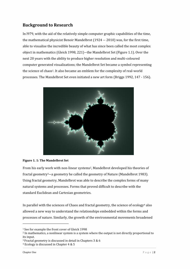
Background to ResearchIn l979, with the aid of the relatively simple computer graphic capabilities of the time,the mathematical physicist Benoir Mandelbrot (1924 ― 2010) was, for the first time,able to visualise the incredible beauty of what has since been called the most complexobject in mathematics (Gleick 1998, 221)―the Mandelbrot Set (Figure 1.1). Over thenext 20 years with the ability to produce higher resolution and multi-colouredcomputer generated visualizations; the Mandelbrot Set became a symbol representingthe science of chaos1. It also became an emblem for the complexity of real-worldprocesses. The Mandelbrot Set even initiated a new art form (Briggs 1992, 147 - 156).
Figure 1. 1: The Mandelbrot SetFrom his early work with non-linear systems2, Mandelbrot developed his theories offractal geometry3―a geometry he called the geometry of Nature (Mandelbrot 1983).Using fractal geometry, Mandelbrot was able to describe the complex forms of manynatural systems and processes. Forms that proved difficult to describe with thestandard Euclidean and Cartesian geometries.In parallel with the sciences of Chaos and fractal geometry, the science of ecology4 alsoallowed a new way to understand the relationships embedded within the forms andprocesses of nature. Similarly, the growth of the environmental movements broadened1 See for example the front cover of Gleick 19982 In mathematics, a nonlinear system is a system where the output is not directly proportional toits input.3 Fractal geometry is discussed in detail in Chapters 3 & 64 Ecology is discussed in Chapter 4 & 5

Chapter One P a g e | 3
the discourse on these relationships and called for the need for the human species tolive in a way that maintained global ecosystems in a state suitable for the maintenanceof all life. This discourse began in earnest with the publication of Silent Spring in 1962(Carson) and was made all the more tangible by the beautiful photograph of the Earthrising over the lunar landscape taken on Christmas Eve, 1968 and published by NASA in1969 (Figure1.2).
Figure 1. 2: Earthrise 24 December 1968― NASA Science Photo LibraryThe impact on the collective human psyche of this image5 was predicted in 1948 by theBritish cosmologist, Sir Fred Hoyle, who thought that the first images of Earth fromspace would change forever how we thought about our own planet ―“ ‘Earthrise’encapsulated the fragility of a place that seems so immense to the people who livethere, but so tiny when viewed from the relatively short distance of its natural satellite[the moon]” (Connor 2009). The effects of Western culture on the seemingly fragileblue-white planet were popularised with the publication of books such as Gaia: A New
Look at Life on Earth (Lovelock 1979) that recognised the Earth as an integratedcomplex system, rather than as a collection of individual components.These new areas of understanding began to mesh with the field of landscape design, sothat by the early 1980s, design professionals began to look for design forms and anaesthetic that reflected this holistic view of Earth and addressed the ecologicalconcerns put forward by the environmental movement. This led several landscapedesign academics and practitioners to propose guiding frameworks for the5 This iconic image was the first time that the Earth has been seen as a planet rather than ashome.

Chapter One P a g e | 4
development of such forms and a corresponding aesthetic. One of the major themescommon to all these frameworks is the recognition of the importance of the dynamicprocesses and resultant structural forms inherent in what are called natural systems6 –that is, systems that are not the result of human endeavour.The growth in understanding of these dynamic processes and the resultant scale-invariance7 of natural systems, led some authors to suggest that fractal geometry couldbecome a referent for these new design forms and an aesthetic that embodied theforms and dynamics of natural systems. This view is supported by recent research thatindicates human perceptual systems have evolved to efficiently process fractalpatterning and that the human species has a visual preference for certain types offractal patterns8. However, how fractal geometry could be used as a referent for designand how to articulate such an aesthetic based on this geometry remained undefined.Combined with this was the recognition that the ‘idyllic pastoral park’ and thePicturesque landscape design forms developed in England during the 18th and 19thcenturies were still extremely influential in Western culture (Howett 1987, 3).Recognising that the picturesque image of nature has become embedded withinwestern culture, Nassauer (1992) identified a dichotomy between the visual structureand form of ecologically healthy landscape and the way we expect them to look. Sheargues that “Landscape structure and ecological function rest upon an armature ofshared social perceptions of the meaning and appropriate treatment of landscape” andthat planned, designed and managed landscapes have to address these perceptions.It is clear that trying to articulating an ecological aesthetic based on the structuralforms and patterns described by fractal geometry is a complex and multi-facetedproblem, which includes understanding the underlying mathematics of fractalgeometry and the philosophy of aesthetics. Similarly, if fractal geometry is the‘geometry of nature’, what is nature? How, given our western cultural heritage of thepicturesque design form, do we distinguish what is a natural environment from anyother?In addition, from the gaps in the initial literature review, it became clear that ourunderstanding of the overall fractal properties of both natural and designed6 The concepts of Nature and natural will be discussed in Chapter 4. For the present discussionthey are used in their normal context.7 See Chapter 38 See the discussion in Chapter 3
Chapter One P a g e | 5
landscapes, as experienced by people every day, was very limited. Filling this gap wasconsidered a key objective of this research if design forms and an aesthetic based onfractal geometry were to be articulated. Therefore, the primary goal of this research,formulated after completing the initial survey of the literature9, was to:Increase our knowledge and understanding of how fractal geometry can beused as a referent for future design forms and the articulation of an aestheticthat can characterise an ecological based approach to landscape design.To achieve this goal, the following questions were formulated as a guide:1. Do different landscape forms, ranging from relatively natural to
highly urban, show a variation in their overall fractal dimension?
2. Is there a statistically significant difference between the fractaldimensions of commonly encountered landscape forms?
3. Can the fractal properties of a landscape be considered as a measureof its ‘naturalness’?
4. Does the use of re-iterated forms at different scales affect the fractaldimension of a landscape?
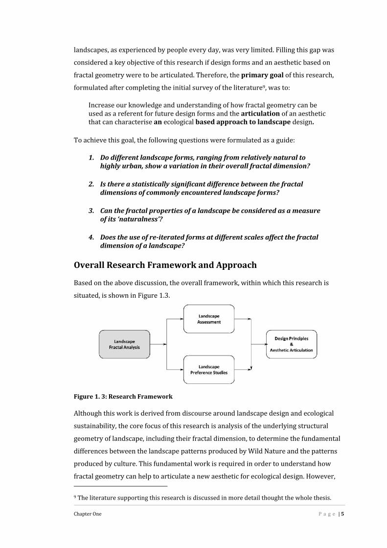
Overall Research Framework and ApproachBased on the above discussion, the overall framework, within which this research issituated, is shown in Figure 1.3.
Figure 1. 3: Research FrameworkAlthough this work is derived from discourse around landscape design and ecologicalsustainability, the core focus of this research is analysis of the underlying structuralgeometry of landscape, including their fractal dimension, to determine the fundamentaldifferences between the landscape patterns produced by Wild Nature and the patternsproduced by culture. This fundamental work is required in order to understand howfractal geometry can help to articulate a new aesthetic for ecological design. However,9 The literature supporting this research is discussed in more detail thought the whole thesis.
Chapter One P a g e | 6
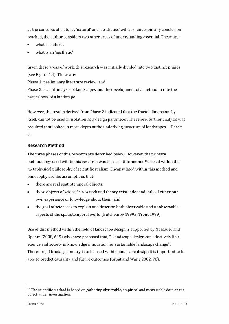
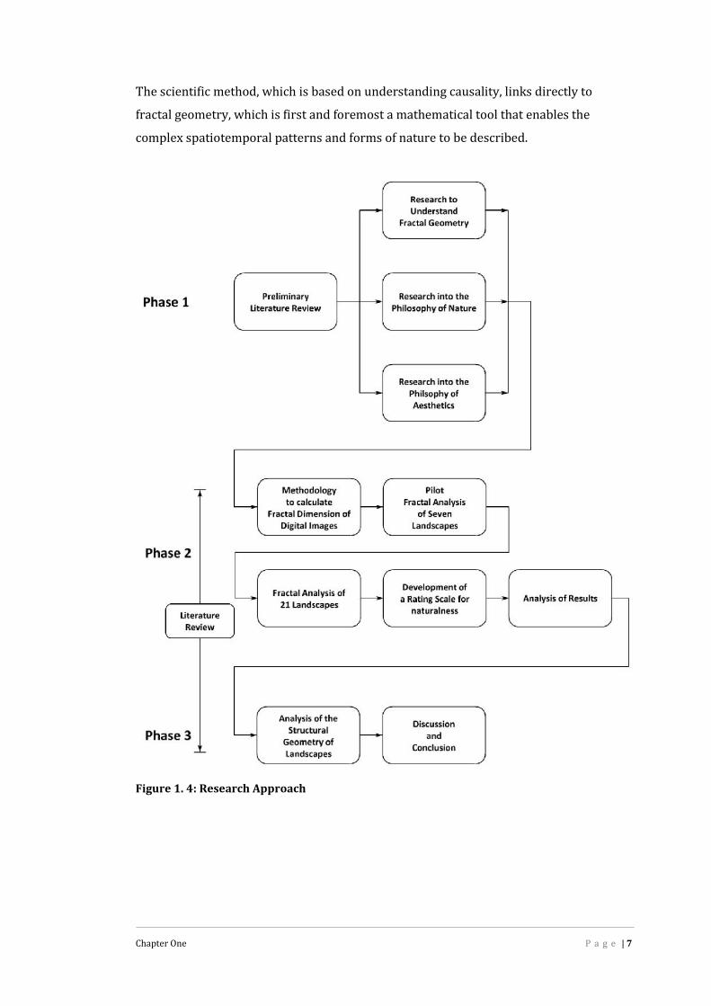
as the concepts of ‘nature’, ‘natural’ and ‘aesthetics’ will also underpin any conclusionreached, the author considers two other areas of understanding essential. These are: what is ‘nature’. what is an ‘aesthetic’Given these areas of work, this research was initially divided into two distinct phases(see Figure 1.4). These are:Phase 1: preliminary literature review; andPhase 2: fractal analysis of landscapes and the development of a method to rate thenaturalness of a landscape.However, the results derived from Phase 2 indicated that the fractal dimension, byitself, cannot be used in isolation as a design parameter. Therefore, further analysis wasrequired that looked in more depth at the underlying structure of landscapes ― Phase3.Research MethodThe three phases of this research are described below. However, the primarymethodology used within this research was the scientific method10, based within themetaphysical philosophy of scientific realism. Encapsulated within this method andphilosophy are the assumptions that: there are real spatiotemporal objects; these objects of scientific research and theory exist independently of either ourown experience or knowledge about them; and the goal of science is to explain and describe both observable and unobservableaspects of the spatiotemporal world (Butchvarov 1999a; Trout 1999).Use of this method within the field of landscape design is supported by Nassauer andOpdam (2008, 635) who have proposed that, “...landscape design can effectively linkscience and society in knowledge innovation for sustainable landscape change”.Therefore; if fractal geometry is to be used within landscape design it is important to beable to predict causality and future outcomes (Groat and Wang 2002, 78).10 The scientific method is based on gathering observable, empirical and measurable data on theobject under investigation.
Chapter One P a g e | 7
The scientific method, which is based on understanding causality, links directly tofractal geometry, which is first and foremost a mathematical tool that enables thecomplex spatiotemporal patterns and forms of nature to be described.
Figure 1. 4: Research Approach

Chapter One P a g e | 8
Phase 1: Preliminary Literature ReviewThis research phase revolved around the concepts of fractal geometry nature, andaesthetics. It became evident that in order to progress this research a clearunderstanding of the mathematical concepts behind fractal geometry was essential.Therefore, the following question required answering.What is fractal geometry?Fractal geometry has been described as the geometry of Nature, but what type ofgeometry is it and what makes it different from other forms of geometry such asEuclidean and Cartesian? This understanding is essential if it is to be used as a referentfor design.Similarly, from the initial literature review it also became clear that the use of the termsnature and aesthetics were confusing. Kim Sorvig (2002, 2) made the astuteobservation that authors in the field of landscape design have tended to be careless intheir use of language and that they should, “evolve away from such over-casualness,and toward a conscious and conscientious use of terms...”. Therefore, as nature andaesthetics are two key components of this research, it was critical that the authoranswer the following questions:.What is Nature?If fractal geometry is the geometry of Nature, it was necessary to examine the conceptof nature within the current western dualistic ideology of culture vs. nature to see ifthere was an alternative approach to understanding humanity’s relationship with thewider spatial and physical world.What is an aesthetic?In much of the landscape design discourse, the word ‘aesthetic’ is often usedinterchangeably with such terms as ‘beauty’ or ‘style’. Similarly, the aesthetic of aparticular design is largely discussed on the basis of an object’s appearance, withoutany reference to the observer.Simon Swaffield (2002, 5) has noted that although landscape architecture has adsorbedmuch from other design disciplines:One important area of differentiation, however, is the central importance ofthe aesthetic and symbolic configuration of geological, hydrological, andbiological forms and processes, and their ecological interrelationships. Thishas always underpinned questions of space and form, and meaning inlandscape architecture, to differing degrees, but in recent decades the

Chapter One P a g e | 9
aesthetics of ecological design and sustainability has emerged as a primaryfocus of interest.Therefore, if an ecological aesthetic is to be developed it was essential to understandwhat is meant by the term ‘aesthetic’.Phase 2: Fractal Analysis of Landscapes and Landscape RatingThis phase of the research collected the primary data through the analysis of digitalphotographic imagery to objectively determine the overall fractal dimension of alandscape. The digital images were collected to represent the visual impressions that auser might experience as they walk within the landscape. Due to the originality of thiswork, it was decided to collect, at a minimum, 20 high resolution digital photographsfrom as many different types of landscape as was practical. However, considerablymore images were required for some landscapes due to their geographic extent.Integral to this research was the development of a specialised software tool thatcalculated the two-dimensional fractal dimension for each digital image. From theseresults the overall median fractal dimension for a landscape was determined.Using this method, 21 landscapes from both within Australia and England have beenstudied, based on a pilot study of seven landscapes within South East Queensland.Phase 3: The Structural Analysis of LandscapesBased on the findings in Phase 1 and the results obtained in Phase 2, the research wasexpanded to enable the rating of each landscape against the new definitions of Naturedeveloped in Phase 1 and further analysis of the underlying structural geometryembedded within each landscape image.Rating the Naturalness of a LandscapeThe question “How natural is this landscape?” is closely aligned to our concepts ofnature, which are discussed in Chapter 4 and vegetation, which is discussed in Chapter7. To compare the fractal dimension of a landscape with an objective measure of‘naturalness’ a simple method to determine the vegetation content within a digitalimage was developed based on a ‘box counting’ system. This method was used todetermine the vegetation content within all images from all landscapes studied. Fromthis an overall Vegetation Rating for each landscape was determined.Analysis of Underlying Structural GeometryThe mathematical tools of Fourier analysis and Kernel Density Estimation were used tofurther characterise the underlying structural geometry embedded within each digital

Chapter One P a g e | 10
image from all landscapes studied. The results of this analysis enabled two newindicators of structural form to be described: the Fourier Power Spectrum MedianAmplitude11 and the level of isotropy12 of the frequency distribution within the Fourierpower spectrum.Research LimitationsPostmodern philosophy questions the assumptions embedded within scientific realism(O'Donnell 2003; Magnus 1999). While recognising that our understanding is limitedby our time and place, there are three main aspects to the limitations embedded withinthis research that are pertinent: those imposed by the physical aspect of the researchmethod itself, those imposed by the knowledge limitations of the author and thoseimposed by the author’s personal biases.Method LimitationsThe limitations imposed by the practical aspects of the research are: The landscapes from within Australia and England analysed are not representativeof all possible landscapes. However, they do represent landscape forms that arecommonly encountered by many people and in particular are the type of subjectsaddressed by many landscape architects. It is recognised that the digital images taken within each landscape do not capturethe complete landscape, but do represent typical visual aspects of that landscape. The method involved taking digital photographs within a specific landscape area. Itis recognised that these photographs only captured elements of that landscape at aspecific point in time. The field of vision of a camera is not equivalent to the binocular vision of thehuman eyes. Measured values for the fractal dimension are dependent upon the mathematicalmodel used to estimate the fractal dimension and the camera. As discussed inChapter 6 there are many different methods used to measure the fractal dimension.The method used to estimate the fractal dimension in this research is based on theFourier Transform. Exact results for each image found in this research could only be repeated if thesame camera was used to record the same images at the same point in time withthe same lighting conditions. However, it is expected that with a different high11 This is the median amplitude of all frequencies within the Fourier power spectrum12 The level of isotropy is how isotropic (same in all directions) the frequency pattern appears.

Chapter One P a g e | 11
quality digital SLR camera taking similar images from within the same landscapesthe results would be proportional and produce similar overall findings to thosefound in this work. The preliminary results from the joint research, noted on pageiii, indicate that this is a valid assumption. While a landscape is experienced through all our human senses as well as throughcognitive understanding and emotional responses, this research only relates to thevisual properties of a landscape created by its underlying structural geometry asexperienced by a user on the ground.Knowledge LimitationsIn attempting to answer the questions relating to Nature and Aesthetics, it must berecognised that the author has never studied philosophy. Therefore, the analysis ofthese key components is, by necessity, kept within the limits of the author’s ability tounderstand the immense amount of philosophical theory and literature that standbehind them. Whether the author has succeeded is for others to decide.Personal BiasQuantum physics teach us that what an ”...observer knows is inseparable from what theobserver is” (Chow 2007, 63) and that there can be no such thing as total objectivity orabsolute truth. Therefore, it must be recognised that the personal biases of the author,derived from his culture, education and life experiences, must be considered to havethe potential to impact the outcomes of this research. This may occur throughinfluencing such elements as: the research method, how the research was conducted,the interpretation of the cited references and the interpretation of the results. Toensure any bias is made clear, the author includes a brief statement of his culturalbackground, values, assumptions and experience.The author is a well educated married male in his mid to late 50’s. He hastravelled extensively within Australia, Europe, the Middle East and the UnitedStates of America. His world view has been shaped by his English upbringing,which would be classified as middle class, and his life and work experiences.Although brought up within the Judeo-Christian belief system, he is withoutany formal religious education and rejects both the creationist belief and thenotion that the human species has dominion over the Earth.Although this research is grounded in the scientific paradigm, his ontologicalbelief system has more in common with Plato’s cave13. He therefore views13 Plato’s Cave refers to the Platonic concept that the sensed material world is just shadows andcopies of Ideal forms that can only be “seen” mentally (Robinson and Groves 2000, 96-98)

Chapter One P a g e | 12
truth and knowledge as relative and that human perception does not assureany understanding of reality.Prior to practicing as a landscape architect he has practised as a bio-medicalengineer specialising in cardiac instrumentation in England, a state managerfor a private company in Victoria and Queensland and a State Governmentemployee in Queensland specialising in GIS systems and knowledgemanagement.Over this research journey he has developed a strong belief in the importanceof philosophy and aesthetics to landscape design and that the WesternNature―culture duality is misleading. He has begun to question the commonconceptions of sustainability and the romantic notion of Nature-as-saviour-inherent within much environmental thought. He also rejects the idea that thehuman species have stewardship over the Earth.Structure of ThesisThis thesis consists of ten (10) chapters, five (5) appendices, additional footnotes and alist of cited references. The main temporal sequence of this research, as shown inFigure 1.4, has been embedded within the structure of the thesis. It has been structuredthis way because it provides a narrative of the author’s journey through this learningexperience and the author considers the journey to be integral to the findings.Chapter 1: Scope of Research ― documents the background, the rationale, the overallresearch approach and the limitations of this work.Chapter 2: Sustainability and Ecological Design ― focuses on the story of our humanimpact on global ecosystems, the concepts of sustainability, the relationship betweendesign and culture and the common themes supporting several frameworks putforward to achieve an aesthetic and structural form for ecological design.Chapter 3: The Patterns of Nature ― describes fractal geometry, what it is, how it wasderived and how it differs from standard Euclidean and Cartesian geometries.Embedded within this is an explanation of the fundamental concept of self-similarity.This chapter also include some discussion on how fractal geometry has been used inthe past, how it is used in the present and the potential problems associated with usingit in the future.Chapter 4: nature or Nature ― understanding what is meant by the terms ‘nature’ and‘natural’ are of fundamental importance if different landscapes are to be compared.Therefore, Chapter 4 briefly examines the philosophy behind our western cultural

Chapter One P a g e | 13
conceptions of nature, the relationship between nature and the human species and theconcepts of ecology. This analysis is used to develop a new model for understandingwhat is meant by nature and what a natural environment is composed of and how thistranslates into geometric forms. It also seeks to describe how the human species and allits activities fit into the overall concept of Nature through the definition of a ‘Para-natural’ environment.Chapter 5: Aesthetics ― reviews the philosophy and principles of aesthetics within thecontext of both art and environment. It also examines the relationship betweenaesthetics, ecology and the environment.Chapter 6: Measuring the Fractal Dimension of a Landscape―extends Chapter 5and discusses in detail the method used to determine the overall fractal dimension ofeach of the 21 landscapes studied in this research.Chapter 7: Rating a Landscape―extends Chapter 4 by defining a landscape as acomposition of both Natural and Para-natural environments. It discusses a new way tocompare landscapes based on the idea of ‘naturalness’ and how this is related to thevegetation content within a landscape.Chapter 8: Fractal Analysis of Landscapes―presents the results obtained throughthe analysis method discussed in Chapter 6 and provides the answers to the researchquestions stated above. This chapter also presents the contributions to knowledgeobtained through the research undertaken to answer each question, the limitation ofthe analysis method discovered through its implementation and suggestions for furtherwork. It also proposes that the fractal dimension by itself is not sufficient to fulfil theprimary goal of this research. Each of the proposed research questions is discussed inthe light of the findings and conclusions presented.Chapter 9: The Geometric Properties of Landscapes―extends this research in a waythat could not have been foreseen at the beginning. Through detailed examination ofthe underlying structural geometry encoded within each landscape, this chapterdescribes two new properties of landscape form. Not only are these properties,encoded within all landscapes, measurable, but this research indicates how they mayrelate to design forms. Conclusions on the relationship of these parameters to abiological basis for some aspects of aesthetics are presented.

Chapter One P a g e | 14
Chapter 10: The Unfinished Landscape―discusses the concept of time and change inrelationship to landscape and presents an overall summary of this research and itsconclusions with respect to fractal geometry and ecological aesthetics. A program forfuture research is also presented.

Chapter Two P a g e | 15
Chapter Two
Sustainability and Ecological Design
Ultimately, the goal of sustainability is the transformation of culture ―the taming of technology, the emergence of a new environmental ethic, a
new measure of life quality, and a substantial broadened sense ofcommunity including not only humans, but all life. (Thayer 2002, 192)
IntroductionDiscourse on the effects of Western culture on natural environments has been ongoingsince at least the late 1800s14. However, with the first publication of Silent Spring in1962, Rachel Carson brought the potentially devastating effect of human actions on theenvironment to public attention. Although there has been major progress inunderstanding the consequences of land clearing and the over use of agriculturalchemicals such as fertilisers, pesticides and herbicides, the human species is still facing(and possibly causing) potentially major ecological changes that could affect thecurrent way of life of most people―particularly in the Western world. However, as NeilEvernden (1992, ix) has observed:It has been thirty years since Rachel Carson alerted us to the ecosystemicdangers of pesticide abuse, yet a rereading of Silent Spring leaves one with thefeeling that little has changed but the names of the poisons.Prior to Rachel Carson’s seminal work, Aldo Leopold had recognised that Westernattitudes towards what he termed “wild things” were a major cause for concern. Theseconcerns, ecological observations and his developing eco-philosophy were published inhis powerful book entitled A Sand Country Almanac and Sketches Here and There, firstpublished in 1949. Leopold’s “land ethic”, based on the principles of ecology, focussedon humankind’s relationship towards the land. He recognised that all biological life, andthe abiotic environment that sustains it, works as an integrated community. Leopoldsaw the future for the human species as re-imaging itself from being the “conqueror ofthe land-community” to being a “plain member and citizen of it”. He regarded the needfor a land ethic to provide direction when ecological conditions arise that are so “newor intricate” that the “path of social expediency is not discernable to the averageindividual”. With this concept of a land ethic, Peter Hay (2002, 15) recognises Leopoldas the first to argue that terms of moral philosophy, derived from Judeo-Christian14 See for example: Marsh 1869, Carson 1962, McHarg 1969, Leopold 1989, Thayer 1994,Papanek 1995, Thompson and Steiner 1997, Phillips 2003

Chapter Two P a g e | 16
religion15, should be extended to include the natural world. With the publication ofpopular books such as GAIA: A New Look at Life on Earth (Lovelock 1979), thediscussions around global ecological issues and how the human species interacts withthe non-human world became far greater than ever before.This Chapter presents an overview of the concept of ecological sustainability and itseffect on landscape design. In this research a landscape is considered to be composed ofone or many environments experienced at a particular scale and design is defined asthe creative process that consciously “redirects and reorganises energy and materials”(Musacchio 2009, 996) in response to some human requirement. This definition ofdesign applies to all professionals and non-professionals who consciously affect theform of a landscape.SustainabilityDiscourse on sustainability began in earnest in 1987, when the United Nations WorldCommission on Environment and Development commissioned a report titled Our
Common Future (WCED 1987), commonly called the Brundtland Report. One of theaims of this report was to propose environmental strategies for achieving globalsustainable development by the year 2000. Within this report sustainable developmentis defined as a...process of change in which the exploitation of resources, the direction ofinvestments, the orientation of technological development; and institutionalchange are all in harmony and enhance both current and future potential tomeet human needs and aspirations.While recognising that development involves progressive changes in both economiesand societies, this report also recognises that development:...tends to simplify ecosystems and to reduce their diversity of species. Andspecies, once extinct, are not renewable. The loss of plant and animal speciescan greatly limit the options of future generations; so sustainabledevelopment requires the conservation of plant and animal species.The concept of sustainability, as defined by the Brundtland Report, has been describedas anthropocentric and biased towards a utilitarianism that recognises the dependenceof the human species upon the rest of the non-human world for its continued existence(Thompson 2000, 18). However, McIvor and McIntyre (2002, 8) propose that the long15 The theological basis for human attitudes towards the natural environment are welldocumented, see for example: White 1967, Thomas 1984
Chapter Two P a g e | 17
term sustainability of the environment is also the ‘ultimate limiting factor’ for humandevelopment. They recognise that an ecosystem cannot be exploited beyond itscapacity to recover. They suggest that, unless we adjust our economic and socialsystems to recognise this, then the global impacts of ecological degradation will adjustour economic and social systems for us. However, as well as economic and socialsystems, philosophy is also playing an important role in the sustainability discourse.Environmentalism and PhilosophyThe growth of global environmental movements, based on eco-centric theories has ledto a major shift in moral philosophy that has begun to challenge one of the underlyingprinciples of the Western value system. That is the belief that morality is a strictlyhuman quality and therefore no moral, or ethical, principle exists to stop humanityfrom behaving in any way it wants towards the non-human world (Hay, P 2002, p17).The new eco-philosophies and green politics now accept that humanity must apply theprinciple of ‘right behaviour’ to all other species (Barry 1994, 371; Berleant 1992, 8-9).The current dichotomy we now face is that the natural world that we have spent solong escaping16 from is now recognised as the very thing that is essential to oursurvival. This recognition is manifested in our concepts of biodiversity and speciesprotection. It is also a principle component of the argument by Emerson (Emerson1991 [1836]) and Suzuki (1997) that wilderness is essential to sustain us spiritually.It is this powerful combination of social and economic factors as well as newphilosophies that is driving the call for a new landscape aesthetic based on ecologicalsustainability ― or as Catherine Howett (1987, 6) so aptly says when discussing thefuture forms of designed landscapes:Surely these new forms must reflect the awakening of our generation toecological consciousness and the growing popular understanding of thedegree to which the natural world is, in Aldo Leopold’s words — interlockedin one humming community of co-operations and competitions, one biota.Design and SustainabilityGiven the growing and widespread ecological concerns, it is not surprising thatlandscape design professionals began to look at how the practice of landscape designand the resultant design structure could change to mirror these concerns and provide16 See Chapter 4

Chapter Two P a g e | 18
practical outcomes to facilitate sustainability. This recognition is reflected in thecurrent Australian Landscape Charter published by the Australian Institute ofLandscape Architects (AILA 2009). This charter sets out five landscape principles that“...articulate an ethical decision-making framework for landscape planning, design andmanagement within the natural and built environment”. Although, in Leopold’s terms,these principles could again be criticised for being too anthropocentric, the recognitionthat landscape architects and designers should “protect existing environmentalfeatures and ecosystems” is fundamentally sound and reflects Leopold’s concerns. Themajor difference being that the AILA charter is primarily focussed on designedlandscapes, whereas Leopold was focussed on maintain what both he and AnneWhiston Spirn have called “wilderness” (Spirn 1947, 4; Leopold 1989, 188). Leopoldsaw wilderness as the “raw material out of which man has hammered the artefactcalled civilisation.” Although this seems to mirror Peter Hay’s (2002, 12) commentswhen he says that “Thus, the history of civilisation can be seen as a history of escapingfrom wilderness; of establishing mastery over it through fire, clearing, cropping,domestication of animals, and so on”, it is clear that Hay’s description of ‘civilisation’ isexactly what Leopold saw as the major problem.Two Approaches to SustainabilitySince the publication of Carson’s and Leopold’s books, further discourse concerning therole of design within the area of ecological sustainability has occurred in and aroundlandscape and other design fields (McHarg 1969; Howett 1987; Koh 1988; Thayer1994; Papanek 1995; Bull 1996; Thompson and Steiner 1997). Denis Cosgrove (2003,15-20) summarised the two main themes within these wider discussions and refers tothem as the ‘ecological’ approach and the ‘semiotic’ approach. He defines the ecologicalapproach to landscape discourse as focussing:... on the complex interactions of natural processes (geomorphological,climatic, biological, vegetational, etc) shaping characteristic land areas andextending its concerns to the ways that human activities interact with thesenatural processes.Within this approach, Cosgrove recognises that modern human interactions with thenatural world are frequently seen as detrimental to maintaining balanced and stablelandscapes. The semiotic approach to landscape discourse he defines as being:...sceptical of scientific claims to represent mimetically real processes shapingthe world around us. It lays scholarly emphasis more on the context andprocesses through which cultural meaning are invested into and shape a

Chapter Two P a g e | 19
world whose ‘nature’ is known only through human cognition andrepresentation and is thus always symbolically mediated.Cosgrove considers the semiotic approach to be “less pessimistic about the future oflandscape” as it situates landscape (and hence landscape design) within the larger fieldof human society and culture.These two approaches are similar to those identified by Simon Swaffield’s (2002, 5) inhis discussion on the role of meaning in design, where he identified two contrastingpositions. On the one hand he sees landscape design as a means to explore the complexsymbolic relationships between human culture, technology and nature. On the otherhand he sees landscape design as a means to achieving “…healthy, functional andpleasurable places for people and communities, to which significance and meaning willaccrue over time”. It is worth noting that both Cosgrove’s and Swaffield’s approachesecho one of the most fundamental arguments in metaphysical philosophy: is realitymaterial and hence objective; or mental and hence subjective (Butchvarov 1999b). Thisdichotomy is also the basis of Evernden’s book The Social Creation of Nature (1992) andthe continuing clash of natures vs. culture. This is discussed further in Chapter 5.Sustainability and Design PracticeToday, the ecological focus of landscape design in Australia is evident in the number ofContinuing Professional Development courses that are offered, such as those on WaterSensitive Urban Design; Bio-Retention System Design, Climate Change Adaptation Skillsand the concept of ‘Green Infrastructure’. However, the rhetoric put forward by theAILA (2011) as part of its landscape principles that: “Human activity threatens thefundamental capacity of landscape to sustain life on earth” fits into the category ofviews about climate change that Lomborg (2008, xi) calls the “unmitigated apocalypseview”. This view is also explicit when authors present the view that the earth is sick ordying (Green 2006, 11). It is clear from the science of paleontological that humanitywould have to go to extreme lengths to extinguish all life on Earth.There can be no doubt that major progress has been made in understanding how builtinfrastructure can contribute to sustainability through such areas as reduction ofcarbon based energy production and water conservation and harvesting in both urbanand rural environments. However, there has been very little discussion on theaesthetics of ecological design or whether aesthetics has a role to play in this designarea.
Chapter Two P a g e | 20
Design and CultureLike all species, the human species has a biological drive to survive and in order to doso we must ensure that the Earth’s ecosystems continue in a state that enables this tohappen. James Corner (1997) has argued that any ecologically focussed landscapedesign must also take into account the role of human culture, as culture is as much apart of nature as all the other areas of life that the science of ecology represent. Afterall, it is Western culture that has created the perceived ecological problems we facetoday, so it must be culture that creates the solution. This is supported by theproposition that culture is now the primary mechanism by which the human speciesadapts to its environment (Sutton and Anderson 2010, 97).The Importance of CultureIn order to achieve a cultural solution, Corner (1997, 99-102) has argued that “Cultureevolves through metaphor and the release of more edifying relationships betweenthings” and that greater use of imagination and metaphor is required to bring thepoetic notion of ‘wonder’ back into landscape design forms. He suggests that ecologicallandscape architecture should not just comprise completion of constructed projects,but be “...more about the design as ‘process’, ‘strategies’, ‘agencies’ and ‘scaffolding’ ―catalytic frameworks that might enable a diversity of relationships to create, emerge,network, interconnect and differentiate”. Ray Green (2006, 16) echoes this view whenhe suggests that the education of landscape architecture students should encompassthe concept of the “poetry of place” by exposing students to both visual art andliterature that embrace ‘landscape’ and ‘place’. However, Corner’s argument goes onestep further, in that it implies landscape design should not just try to mimic thestructure of natural environments, but should parallel natural processes and how theyrespond to environmental change; allowing new systems and structures to evolve.Therefore, as the survival of the human species is dependent on healthy andfunctioning natural systems and processes, it is these systems and processes that mustbe integrated with human culture in any design intervention.In her book Landscape Design: A Cultural and Architectural History, Elizabeth BarlowRogers (2001, 20-21) recognises that to understand designed landscapes it is firstnecessary to understand the philosophical, religious, scientific, technological, politicaland economic ideas that drive a particular culture at any period in history, as it is thesecultural values that are reflected in the design structure. The designs that Rogers hasdocumented as being driven by the cultural values of their time include the absolutist
Chapter Two P a g e | 21
and geometric designs of Le Notre (1613-1700), the idealised English landscapegardens of William Kent (1684-1748), Lancelot ‘Capability’ Brown (1716-1783),Humphrey Repton (1752-1818) and John Loudon (1783-1843), and the Modernistdesigns of Thomas Church (1902-1978) and Garret Eckbo (1910–2000).Design and AdaptationThis recognition of the importance of culture to design is supported by CatherineHowett (1987, 4) and is expanded by James Corner (1999, 1) when he proposes that adesigned landscape is not just a reflection of a culture, but has the power to activelyshape culture by connecting with the “metaphysical and political programs that operatein a given society”. The concept that a designed landscape can proactively changeculture is powerful and in some respects can be seen in the effect of the Englishlandscape park and picturesque design forms in changing people’s conception ofNature at that time―albeit a heavily modified Nature. Thayer (1976, 40) addressed thiswhen, recognising that ecological concerns were causing a shift in the way people sawtheir environment, he suggested that it is the profession of landscape architecture that“...will bear the responsibility of making aesthetic sense out of this attitudinalmetamorphosis”. In other words, if attitudes towards the natural environment arechanging there is now a need for an aesthetic that can bridge the gap between theecological ‘ideal’ and the practical ‘real’ in landscape design, in much the same way thatthe aesthetics of the pastoral park and the picturesque was an attempt to deliberatelyreconstruct “the chance effects of nature” (as noted in the Oxford Dictionary of Art(1970, 1008)).What is clear from Rogers’ analysis of the historic development of landscape design isthat past design structures have always provided inspiration for contemporarylandscape designers within any period. This view is supported by both ChristopherThacker in his book The History of Gardens (1979, 83-84) and more fully in theexploration of the English landscape garden by John Dixon Hunt and Peter Willis(1988). However the danger, according to James Corner (1991, 120), in blindly usingforms from the past, is that these forms can become empty shells, or stencils, that nolonger house the philosophical or cultural meaning relevant to their time of origin.Marc Trieb (1995, 49) echoes this view when he says, with some sarcasm:One can almost hear designers saying, sotto voice: ‘If they meant something inthe past (of course, we have to like them as forms...), then they will meansomething again to us today.

Chapter Two P a g e | 22
John Dixon Hunt (Hunt 1991, 20) takes an alternative view and sees historic designforms as being, in a sense, capable of multi-cultural and multi-temporal adaptation,where the structure remains similar but the effective content changes. He uses theexample of the sixteenth and 17th century Italian gardens and how they became a majorsource of inspiration for garden design and cultural expression across England andmost of northern Europe; even though social, cultural and climatic conditions werevery different.This potential for historic design forms to be adapted across culture and time has beenrecognised by Catherine Howett (1987, 3). She argues that the designs of Frederick LawOlmsted (1822-1903) were inspired by the “powerful inherited models” of the Englishidyllic pastoral park, which, she suggests, are the “quintessential emblem of a civilised,humanised natural world…”. It was these English design forms that enabled Olmsted tofulfil his own social and philosophical program for New York’s Central Park and otherprojects. Louise Mozingo (1997, 54) has argued that the continuing public resonance ofthe landscapes of Olmsted and Vaux lies in no small part in their ability to structurecomplexity with clarity.Given the dynamic complexity of ecological systems and the human need to “combatuncertainty and maintain control” (Galinsky and Whitson 2008, 115) one of the mainproblems that faces landscape design today is to allow the ecological systems thathumans depend on to evolve as natural expressions of an holistic but extremelycomplex world, while still enabling that sense of control, through clarity of design, thatwe humans require within our overall environment. Aesthetics has been identified asone of the primary aspects within the field of design that can assist in helping achievethis outcome (Richards 2001; Musacchio 2009).Frameworks for Ecological DesignCatherin Bull (1996, 27) argued that the content of landscape design is “nature”. If thisis the case, what physical form should a sustainable landscape take? Howett (1987, 6)recognises that this is a question without an answer and proposes that any new formswill “emerge from the play of mind and spirit, from risk taking experiment andpainstaking work”.With ecological sustainability one of the major philosophical and political programs ofmodern western society, James Corner (1997, 82-83) has suggested that

Chapter Two P a g e | 23
What is important and significant here is how ecology and landscapearchitectural design might invent alternative forms of relationships betweenpeople, place, and cosmos. Thus, the landscape architectural project becomesmore about the invention of new forms and programs than merely correctivemeasures of restoration.In recognition that landscape design has the potential to achieve a paradigm shift in theway people perceive and interact with both the natural and built environments, severalauthors have proposed conceptual frameworks for the development of new structuralforms and relationships for ecological design (Bull 1996; Howett 1987; Koh 1988;Mozingo 1997; Musacchio 2009; Nassauer 2002; Spirn 1988; Thwaites 2000; Nohl2001; Meyer 2008). A review of these frameworks highlighted some common themesthat run through most, if not all of them. These are synthesised and outlined below.Aesthetics as an Agent of TransformationThe structural forms of designed landscapes today are considered to be based on theaesthetic theory and principles of composition developed during the eighteenth andnineteenth centuries. It is these theories that underlie the structure of the Englishpastoral park and the picturesque design forms that inspired later designers and arestill considered to be a powerful influence on current design practice. This culturallydetermined aesthetic focus is now considered inappropriate for a design structure thatneeds to reflect both ecological and cultural sustainability. However, it is recognisedthat the alliance between the picturesque aesthetic and ecological processes, evident inthe designs of Olmsted, require further exploration.These frameworks recognise that a positive aesthetic response to a design can have adirect effect on cultural attitudes. This has been shown to be evident with the Englishlandscape tradition that changed Western cultural attitudes to accepting a certainstructural and spatial form of Nature. However, an ecological aesthetic must bebroadened so that its focus is not tied to artistic principles, but includes a greatercognitive understanding of the ecological processes that bind the human species to thebroader ecosphere. An aesthetic of sustainability must bridge the gap between thescience of ecology and art.Re-connecting Humanity and NatureThe dualistic conception of humanity and its various cultures as being somehowseparate from the rest of Nature is recognised as a Western ideology that is a majorobstruction to the achievement of ecological sustainability. This ideology needs to be

Chapter Two P a g e | 24
abandoned so the reality that humanity and Nature are indivisibly connected within asingle continuum is communicated through designed landscapes.The Dynamic Processes and Structural Forms of NatureCurrent landscape design structures are acknowledged as being static. They are basedon Euclidean and Cartesian geometries that are abstractions of the spatial and physicalworld, through which the concept of time and the natural process of regenerationthrough birth, life, death and decay are removed. However, Nature is a dynamic forcethat creates self-similar structural forms and patterns through the infinitecombinations of order and disorder. These self-similar forms and patterns are alsodiscernable in the older urban districts throughout the world created by humanculture; therefore, it is no coincidence that these old urban environments are describedas ‘organic’.The patterns and structures created by these dynamic processes, and their similarityacross all scales of existence are described by fractal geometry. It has been proposedthat this new geometry of Nature may become a referent for an approach to ecologicaldesign (Baird 2002) that can embody the dynamic processes that are so essential forlife (Spirn 1988).Ecological Design and Landscape Practice
A recent study into landscape design practice in the United States of America byKatherine Crewe and Ann Forsyth (2003) developed a typology of six differentapproaches to landscape design. The attitude towards Nature within these approaches isshown in Table 2.1 (Summarised from Crewe and Forsyth 2003)Table 2. 1: Approaches to Landscape Architectural Practice
Design Approach Attitude to Nature
Design as Synthesis The intrinsic value of nature is not considered, solutions tohuman problems are paramount
Cultivated Expression Plants, as part of nature, are a means of artistic expression,combined with other materials
Landscape Analysis Nature is either an intrinsic focus or protected because of itsvalue to human society
Plural Design Nature as setting for human life
Ecological Design Respects the natural world and creates landscapes that createhuman-scaled ecosystems
Spiritual Landscapes Nature is a setting for the human spiritual and transcendentdimensions of life

Chapter Two P a g e | 25
At the time this study was undertaken, it became apparent to the authors that the‘Design as Synthesis’ was the approach generally used to develop a design structure.Within this approach the intrinsic worth of the natural environment came second tosolving the human problems identified within the design brief. Of the two approacheslinked to natural environments, the ‘Landscape Analysis’ approach was found to befocussed on the management and conservation of the natural environment and the‘Ecological Design’ approach focussed on either restoration of the natural environmentor trying to achieve a balance between natural and human systems.This inability of contemporary landscape design practice to convert the ideas andtheories discussed above into viable design outcomes highlights the complexity of theissue and the ongoing gap between design theory and design practice.ConclusionIt is clear from the preceding discussion that the current aesthetic ideals withinWestern culture are not considered appropriate for a landscape design form that isboth sustainable in the short term and capable of symbolising the proposed re-connection of humanity and Nature that is required over the long term. Similarly, theabstractions of spatial and physical reality represented by Euclidean and Cartesiangeometries are considered inherently static. The static nature of these geometries areseen as inappropriate for developing new design forms and an aesthetic that encodesthe dynamic and inherent activity of natural systems that drive the cycle ofregeneration required for life. To overcome this deficiency, fractal geometry, whichdescribes the patterns formed by natural systems and processes, has been proposed asan alternative design referent.Fractal geometry and its relationship to the standard Euclidean and Cartesiangeometries is discussed in the next chapter.

Chapter Three P a g e | 26
Chapter Three
The Patterns of Nature
The new geometry mirrors a universe that is rough, not rounded,scabrous, not smooth. It is a geometry of the pitted, pocked, and broken
up, the twisted, tangled and intertwined. (Gleick 1998, 94)
IntroductionAlthough Baird (2002) and Spirn (1988) have proposed that fractal geometry couldform a referent for new design forms no indication is given in their writings as to howthis form of geometry can be translated into design practice. This is not reallysurprising given the complexity of fractal geometry and its relationship to Nature andaesthetic theory. However, Sorvig (2002, 10), in his discussion on design form, is veryspecific in his call for all writers (and it would be appropriate to add all designers), tobecome familiar with fractal geometry, as he considerers it to be “one of the mostvaluable concepts available for discussing landscapes.”Fractal geometry is first and foremost a mathematical language of geometry. Yet itsmost basic elements cannot be viewed or used directly. In this aspect it differs from thefamiliar Euclidean and Cartesian geometries, which are based on points, lines, circles,polygons, solids and orthogonal axis (Jurgens et al. 1990). However, to understand theconcept of fractal geometry it is first necessary to understand the concept of dimension.In the traditional three-dimensional Euclidean and Cartesian space dimension isunderstood through the location of a point within that space. However, dimension canalso be defined by scale (Mandelbrot 1983, 30) and it is the mathematics of scale baseddimension that leads directly to fractal geometry and the concept of self-similarity.Dimensions of SpaceThe mathematical study of dimensions is a very complex area and a completedescription of the subject is beyond both this thesis and the author. However, someunderstanding of the notion of dimension and how this relates to our commonunderstanding of space17 and geometry is required.In 1783 Immanuel Kant (2008 [1783], 33-34) wrote17 The term ‘space’ refers to the boundless, three-dimensional extent in which objects andevents occur and have relative position and direction of movement

Chapter Three P a g e | 27
That everywhere space (which (in its entirety) is itself no longer theboundary of another space) has three dimensions, and that space cannot inany way have more, is based on the proposition that not more than three linescan intersect at right angles in one point; but this proposition cannot by anymeans be shown from concepts, but rests immediately on intuition, andindeed on pure and a priori intuition, because it is apodictically18 certain.With this one statement, Kant encapsulated the mathematical concepts of Euclidian andCartesian three dimension space that is taught in schools and, it is probably true to say,are still the most widely used systems of geometry today. But what is a dimension?The Three Dimensions of Euclidean GeometryEuclidean geometry is the earliest mathematical system that logically andsystematically discusses geometry as we understand it today. Euclid’s geometry isbased on a series of axioms19 that encompasses the description of such things asstraight lines, circles, parallel lines and triangles and Platonic forms such as cubes,spheres and cylinders. Within Euclidean geometry everything exists within a threedimensional space, which is a representational model of the physical universe that isknown to exist.Physical space can be considered to consist of an infinite number of unique points,where a point has no actual size but represents a specific location within that space.Classically, in both mathematics and physics, the dimension of a space, or an object, is apositive integer20 which represents the minimum number of coordinates required toidentify the location of a point in space or on an object. In mathematics there are manydifferent types of coordinate systems that can be used to locate a point in space; forexample, the Cartesian system, the Polar system and the Spherical system.Figure 3.1 shows how this works for the most common―the Cartesian system.
18 Apodictically refers to something that is incontestable as it is able to be demonstrated19 An Axiom is a proposition that does not require proof as it is self-evident.20 A positive integer is any whole number such as 1, 2, 3, 4, 5 etc

Chapter Three P a g e | 28
Figure 3. 1: Cartesian Three Dimensional SpaceHere the point of origin, shown by the black dot, represents a location in space. Thispoint has a dimension of zero as the point does not really exists as an object, but is thesymbolic representation of that particular location. If we drag that point in a particulardirection (X), we can join the two points by a line. To locate a point ‘p’ along the line weonly need to measure the distance ‘a’ from the origin point to the point ‘p’. Therefore, tolocate ‘p’ we only need one coordinate―hence a line is considered one dimensional. Ifwe now drag the line in a direction (Y), 90 degrees to the original line we create a plane.To locate a point on that plane we now require two coordinates, as the point is locatedat a distance ‘a’ along direction X and a distance ‘b’ along direction Y―hence a plane isconsidered two dimensional. If we now drag the plane in a direction (Z) 90 degrees tothe original plane we create a volume. To locate a point inside the volume we now needthree coordinates, as the point is located at a distance ‘a’ along the X direction, ‘b’ alongthe Y direction and ‘c’ in the Z direction―hence a volume is three dimensional. Thesethree dimensions are also known as the ‘Topological’ dimensions.One of the counter-intuitive things about three dimensional space is that although avolume is three dimensional, because it requires three coordinates to locate a pointwithin it, any point on its surface only requires two coordinates to locate it, thereforethe surface of the volume is two dimensional. This is why we only need themeasurements of Latitude and Longitude to locate any point on the surface of theEarth, as the Earth is an almost spherical, three dimensional volume within cosmicspace. However, its surface is effectively a two dimensional plane, as shown in Figure3.2.

Chapter Three P a g e | 29
Figure 3. 2: Latitude and Longitude Coordinate System21Because Euclidean and Cartesian geometries are based on locating a point within 3-dimensional space, they are the ideal geometries for generating and describing objectssuch as the British Library, London shown in Figure 3.3 as they allow structures such asthese to be drawn, measured and physically constructed.
Figure 3. 3: The British Library
The Hausdorff DimensionAnother way to define dimension, based on scaling rather than defining location, wasdeveloped in 1918 by the mathematician Felix Hausdorff, to help understand veryirregular mathematical shapes that did not quite fit the Euclidean and Cartesianmodels. Figure 3.4 helps to explain how scaling dimensions using the Hausdorff methodare determined.
21 Image based on drawing by Geek3, Wikipedia
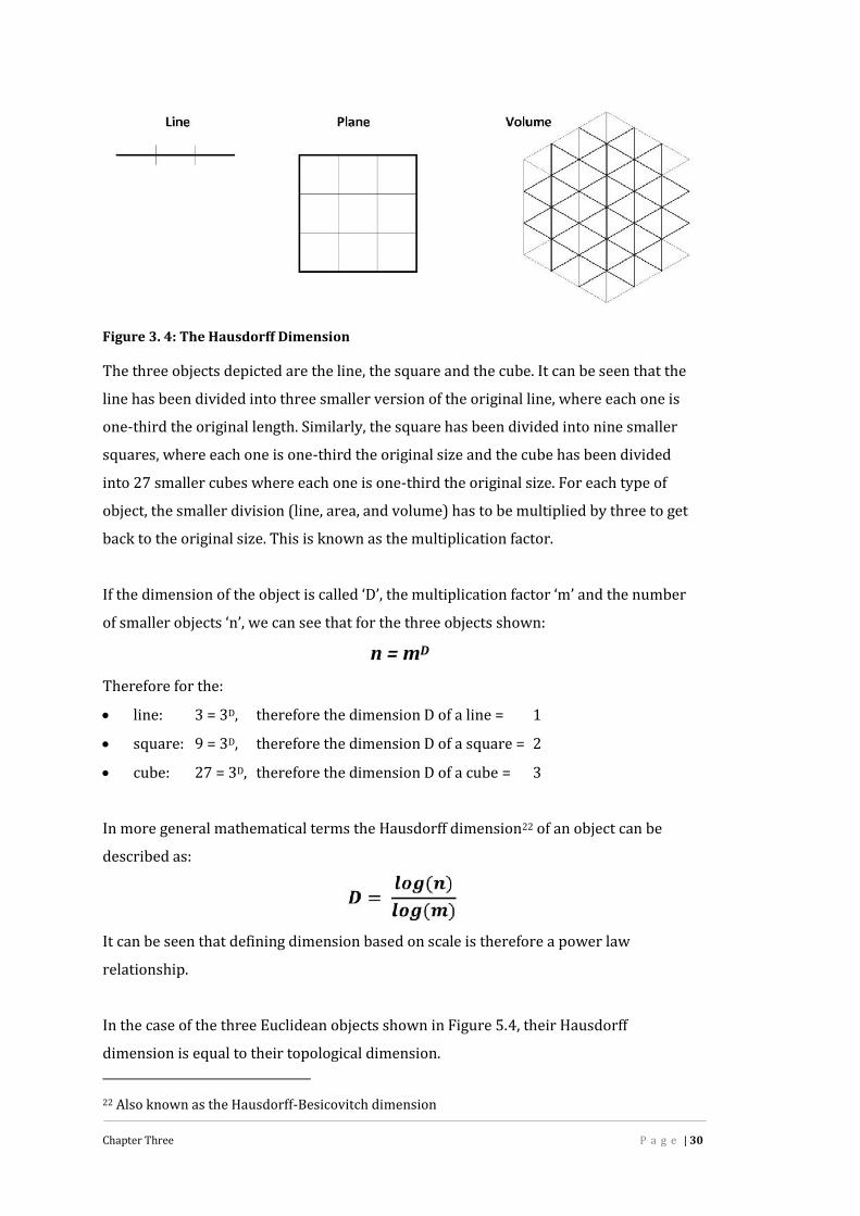
Chapter Three P a g e | 30
Figure 3. 4: The Hausdorff DimensionThe three objects depicted are the line, the square and the cube. It can be seen that theline has been divided into three smaller version of the original line, where each one isone-third the original length. Similarly, the square has been divided into nine smallersquares, where each one is one-third the original size and the cube has been dividedinto 27 smaller cubes where each one is one-third the original size. For each type ofobject, the smaller division (line, area, and volume) has to be multiplied by three to getback to the original size. This is known as the multiplication factor.If the dimension of the object is called ‘D’, the multiplication factor ‘m’ and the numberof smaller objects ‘n’, we can see that for the three objects shown:
n = mDTherefore for the: line: 3 = 3D, therefore the dimension D of a line = 1 square: 9 = 3D, therefore the dimension D of a square = 2 cube: 27 = 3D, therefore the dimension D of a cube = 3In more general mathematical terms the Hausdorff dimension22 of an object can bedescribed as:It can be seen that defining dimension based on scale is therefore a power lawrelationship.In the case of the three Euclidean objects shown in Figure 5.4, their Hausdorffdimension is equal to their topological dimension.22 Also known as the Hausdorff-Besicovitch dimension

Chapter Three P a g e | 31
Monster Curves and Self-SimilarityFrom the late 19th century, mathematicians discovered particular types of curves thatexhibited highly complex and irregular shapes. The curves were formed through aprocess called iteration23 and because of their structural properties became known as‘monster curves’. The concept behind iteration can be easily visualised by standingbetween two mirrors parallel to each other. The reflection in each mirror is repeated aninfinite number of times as it bounces back and forth between the mirrors; eachrefection contains multiple reflections from the other mirror. This effect is shown inFigure 3.5.
Figure 3. 5: Visual Iteration24The first example of these monster curves was discovered by the mathematicianGiuseppe Peano in 1809 (Crilly 2007, 91) and is called a ‘space-filling’ curve. The term‘space-filling’ describes the fact that the final (infinite) iteration of the curve connectsevery point in a space without crossing itself. The Hilbert Curve, described by the23 Iteration is a mathematical operation that takes the preceding value of ‘something’ within aprocess and uses that value to calculate the next value. Recursion is a form of iteration.24 Image from http://www.umpi.maine.edu/info/nmms/mirrors.htm. Copyright permissiongranted.
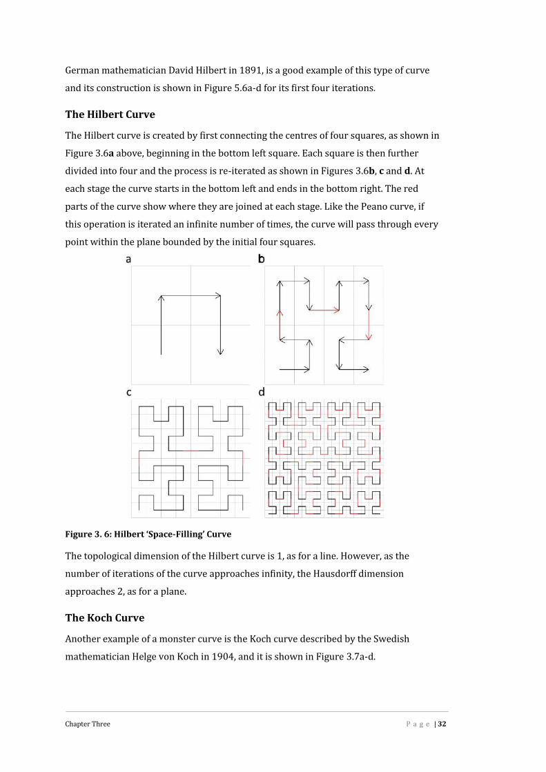
Chapter Three P a g e | 32
German mathematician David Hilbert in 1891, is a good example of this type of curveand its construction is shown in Figure 5.6a-d for its first four iterations.The Hilbert CurveThe Hilbert curve is created by first connecting the centres of four squares, as shown inFigure 3.6a above, beginning in the bottom left square. Each square is then furtherdivided into four and the process is re-iterated as shown in Figures 3.6b, c and d. Ateach stage the curve starts in the bottom left and ends in the bottom right. The redparts of the curve show where they are joined at each stage. Like the Peano curve, ifthis operation is iterated an infinite number of times, the curve will pass through everypoint within the plane bounded by the initial four squares.
Figure 3. 6: Hilbert ‘Space-Filling’ CurveThe topological dimension of the Hilbert curve is 1, as for a line. However, as thenumber of iterations of the curve approaches infinity, the Hausdorff dimensionapproaches 2, as for a plane.The Koch CurveAnother example of a monster curve is the Koch curve described by the Swedishmathematician Helge von Koch in 1904, and it is shown in Figure 3.7a-d.

Chapter Three P a g e | 33
This curve is constructed by taking a line and dividing it into three segments of equallength, as shown in Figure a above. Then an equilateral triangle is drawn that has themiddle segment from step a as its base and points outward. The line segment that is thebase of the triangle is then removed as in Figure b. This process can then be repeatedfor each line segment as shown in Figures c to e above. The Koch curve has infinitelength because each time step c is undertaken, for each line segment, four times thenumber of line segments are generated (n=4). At each stage the new line segments areone-third the length of the segments on the preceding stage (m=3), therefore, after eachiteration, the total length of the curve increases by one-third.
Figure 3. 7: Koch CurveLike the Hilbert curve, the Koch curve has a topological dimension of 1. However, asthis curve is not space-filling and based on the examples shown in Figure 3.4, it can beseen that with every iteration of the division of a line segment n becomes 4 and mbecomes 3. Therefore, the Hausdorff dimension of the Koch curve is:
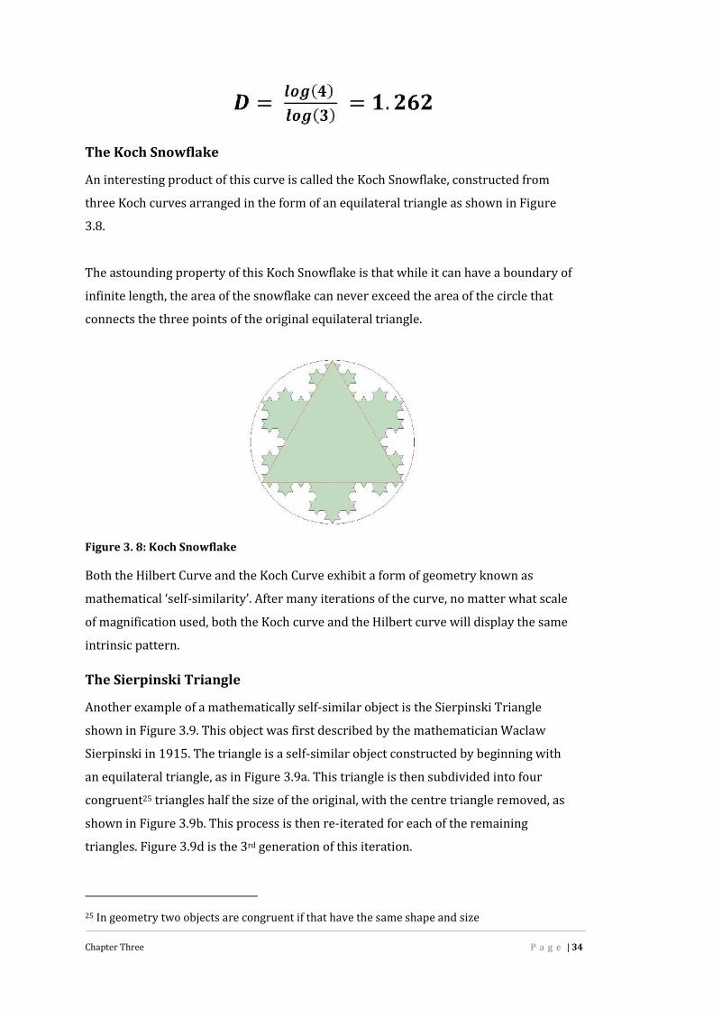
Chapter Three P a g e | 34
The Koch SnowflakeAn interesting product of this curve is called the Koch Snowflake, constructed fromthree Koch curves arranged in the form of an equilateral triangle as shown in Figure3.8.The astounding property of this Koch Snowflake is that while it can have a boundary ofinfinite length, the area of the snowflake can never exceed the area of the circle thatconnects the three points of the original equilateral triangle.
Figure 3. 8: Koch SnowflakeBoth the Hilbert Curve and the Koch Curve exhibit a form of geometry known asmathematical ‘self-similarity’. After many iterations of the curve, no matter what scaleof magnification used, both the Koch curve and the Hilbert curve will display the sameintrinsic pattern.The Sierpinski TriangleAnother example of a mathematically self-similar object is the Sierpinski Triangleshown in Figure 3.9. This object was first described by the mathematician WaclawSierpinski in 1915. The triangle is a self-similar object constructed by beginning withan equilateral triangle, as in Figure 3.9a. This triangle is then subdivided into fourcongruent25 triangles half the size of the original, with the centre triangle removed, asshown in Figure 3.9b. This process is then re-iterated for each of the remainingtriangles. Figure 3.9d is the 3rd generation of this iteration.25 In geometry two objects are congruent if that have the same shape and size
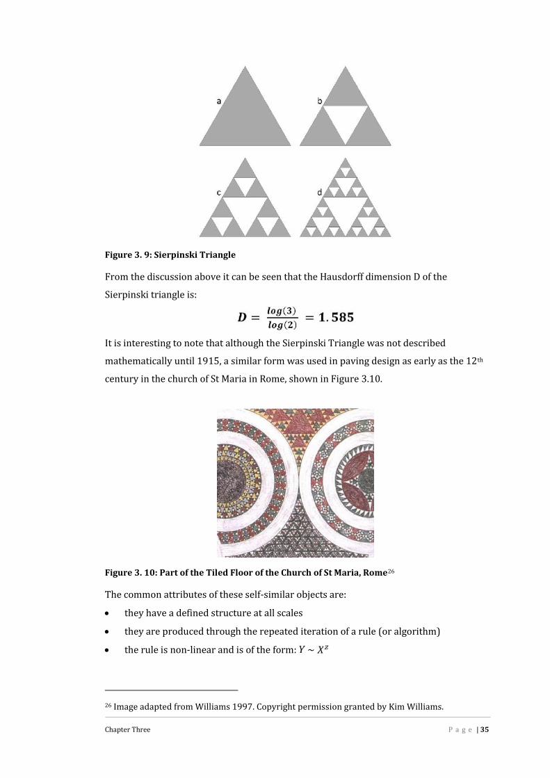
Chapter Three P a g e | 35
Figure 3. 9: Sierpinski TriangleFrom the discussion above it can be seen that the Hausdorff dimension D of theSierpinski triangle is:It is interesting to note that although the Sierpinski Triangle was not describedmathematically until 1915, a similar form was used in paving design as early as the 12thcentury in the church of St Maria in Rome, shown in Figure 3.10.
Figure 3. 10: Part of the Tiled Floor of the Church of St Maria, Rome26The common attributes of these self-similar objects are: they have a defined structure at all scales they are produced through the repeated iteration of a rule (or algorithm) the rule is non-linear and is of the form: ~26 Image adapted from Williams 1997. Copyright permission granted by Kim Williams.
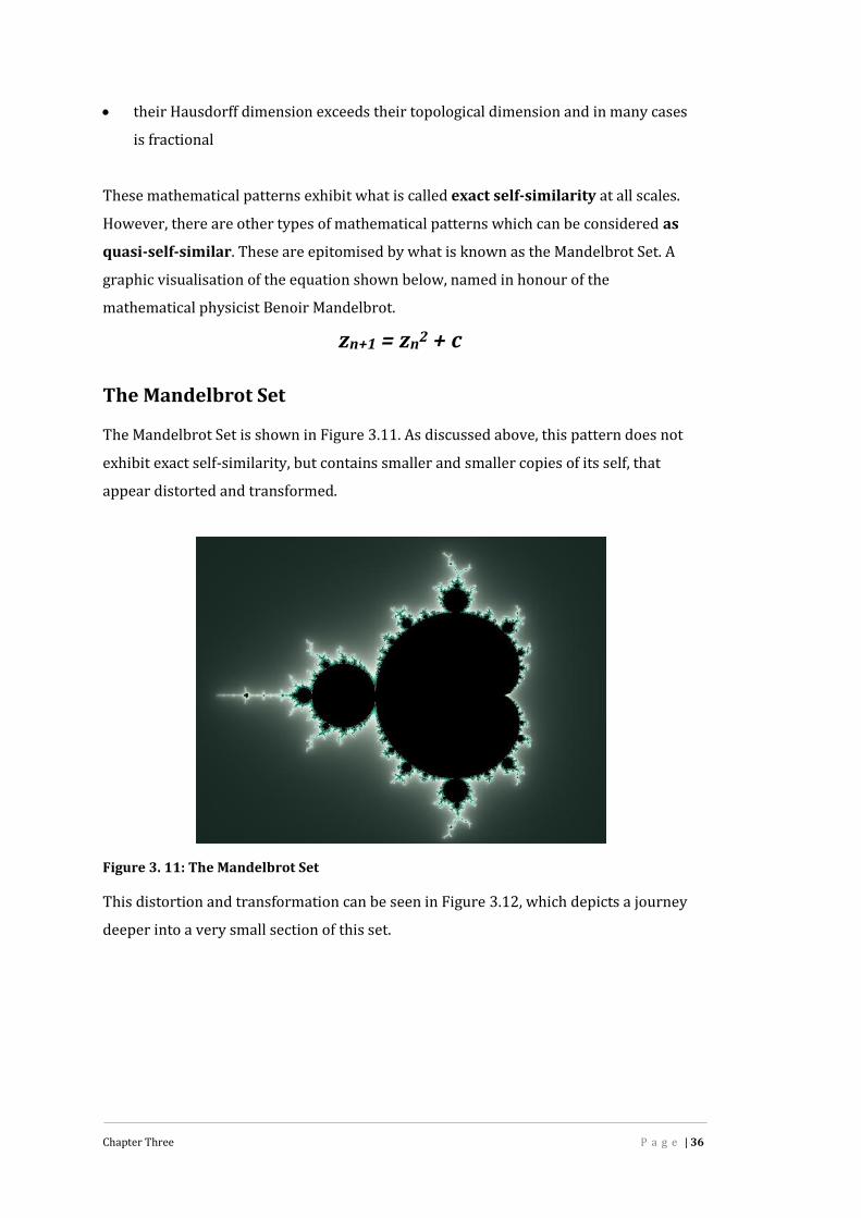
Chapter Three P a g e | 36
their Hausdorff dimension exceeds their topological dimension and in many casesis fractionalThese mathematical patterns exhibit what is called exact self-similarity at all scales.However, there are other types of mathematical patterns which can be considered as
quasi-self-similar. These are epitomised by what is known as the Mandelbrot Set. Agraphic visualisation of the equation shown below, named in honour of themathematical physicist Benoir Mandelbrot.zn+1 = zn2 + c
The Mandelbrot SetThe Mandelbrot Set is shown in Figure 3.11. As discussed above, this pattern does notexhibit exact self-similarity, but contains smaller and smaller copies of its self, thatappear distorted and transformed.
Figure 3. 11: The Mandelbrot SetThis distortion and transformation can be seen in Figure 3.12, which depicts a journeydeeper into a very small section of this set.

Chapter Three P a g e | 37
Figure 3. 12: A Journey Through the Mandelbrot SetThe yellow rectangle in each section of Figure 3.12 represents the area zoomed into inthe next image. The equivalent spatial magnification is around 108, which is1:100,000,000.The Mandelbrot Set is composed of a set of points in what is known as the complexplane, where the boundary of the set forms a fractal pattern. Thus the actual Set isrepresented by the black regions within the Figure 5.12.As stated above, the set is produced from the equation:
zn+1 = zn2 + cWhere z is a complex number of the form:z = x + iywhere i = square root of -1
For example, with a starting value of z =0 and c = 1, this produces the sequence ‘0, 1, 2,5, 26, 677, 458330,…,’, which can be seen results in a number sequence that steadily

Chapter Three P a g e | 38
and quickly grows towards infinity. Therefore 1 is not an element of the MandelbrotSet. However, if c = i the sequence becomes 0, i, (−1 + i), −i, (−1 + i), −i…, whichproduces a sequence that oscillates between two points (-1 + i) and –i, and therefore ifalls within the Mandelbrot Set.The visual form of the fractal boundary of the Mandelbrot Set27 is based on the numberof iterations it takes to determine whether an initial starting condition remains insideor outside the set, and how many iterations it takes for it to tend towards infinity. Themain characteristics of the Mandelbrot Set are: it has defined structure at all scales the structures at different scales are similar but differentAs discussed, exact self-similar and quasi-self-similar patterns are generated throughmathematical processes. However, in the late 1970s, Mandelbrot (1983) discoveredthat a form of self-similar pattern is produced by the systems and processes of Nature(Mandelbrot 1983; Briggs 1992; Gleick 1998; Jurgens et al. 1990; Pentland 1984;Ruderman and Bialek 1994; Spehar et al. 2003; Li 2000). After Mandelbrot publishedhis findings, these self-similar forms became known as fractals and the Hausdorffdimension ‘D’, described above, became known as the fractal dimension. Mandelbrotcreated the term fractal geometry, as distinct from the standard Euclidean andCartesian geometries because it enabled the description of patterns created by exactand quasi-self similar forms whose dimensions were not exact intergers.Fractal GeometryFractal geometry is first and foremost a mathematical language28 of geometry;however, unlike Euclidean geometry which is composed of points, lines, planes andvolumes, the basic element(s) of fractal geometry cannot be distinguished as separateentities. As discussed above the patterns described by fractal geometry are derivedthrough an iterative process. In mathematical systems, these processes are encoded inthe rule or algorithm used to generate the patterns; in biotic systems, these processesare built into the genetic code of the life form; in abiotic systems they are the result ofthe physical laws of the Cosmos.27 For a relatively easy to understand description of how the image for the Mandelbrot Set iscreated see http://warp.povusers.org/Mandelbrot/28 For a discussion of mathematics as a language seehttp://www.fdavidpeat.com/bibliography/essays/maths.htm

Chapter Three P a g e | 39
What Mandelbrot discovered, is that many natural systems and entities have anunderlying geometric order that results from this self-similarity29 which can be eitherspatial or temporal, depending on the object, system or process being examined. It isthe ability of fractal geometry to describe and quantify the self-similar complexity ofnatural forms, (as exemplified by the Romanesco Broccoli shown in Figure 3.13, whichseparates fractal geometry from Euclidean and Cartesian geometries.
Figure 3. 13: Romanesco Broccoli (Brassica oleracea [Botrytis group])
The Length of a CoastlineTo illustrate his ideas, Mandelbrot initially used the concept of measuring the length ofthe coast of Britain. Mandelbrot based this work on earlier studies by Lewis Richardson(Mandelbrot 1983, 28-29). Mandelbrot realised that there is no such thing as a truelength of a coastline, because the smaller the unit of measurement used, the longer thecoastline became. This is illustrated in Figure 3.14 and Table 3.1 based on a length ofthe Hervey Bay coastline in Queensland, Australia.
29 Self-similarity is synonymous with the term scale-invariance

Chapter Three P a g e | 40
Figure 3. 14: Coastline LengthFigure 3.14 depicts the measurement of the coastline between Burrum Heads andUrangan. The red line is the initial starting measurement using a line length of 30km.The purple line estimates the length with a line of 15km; the yellow with a line of 5km;the green with a line of 1km and the blue with a line of 0.5km. These lines are theequivalent of the “Divider-Compass” method of analysis and are summarised in Table3.1.Table 3. 1: Coastline Measurement
Colour Line Length (km) Estimated Coast Length (km) % IncreaseRed 30 30 0Purple 15 31 3.3Yellow 5 31.5 5Green 1 35.8 19.3Blue 0.5 41.8 39.3
It can be seen that as the length of line used to estimate the length of the coastlinebecomes smaller, the length of the coastline becomes larger. Therefore the length of thecoastline is dependent on the scale of observation. As the length of the line used toestimate the length of the coastline tends to zero, the length of the coastline will tendtowards infinity. This is similar to the Koch Snowflake shown in Figure 5.8.Mandelbrot interpreted coastlines as approximate fractal curves and estimated theslope of the regression line for the data plotted on a log-log scale to be equal to 1-D.This is been shown in Figure 3.15.

Chapter Three P a g e | 41
Figure 3. 15: Coastline Data Plotted on Log-Log AxisThe slope of this line is -0.1175. Therefore the fractal dimension D for the length of thecoastline is 1.1175. Thus, coastlines are not Euclidean forms but are highly complexshapes. However, the additional factor that Mandelbrot did not address is that they arealso dynamic entities and are continually changing as a result of the action of tides,erosion and accretion. Therefore, any estimate of the length of a coastline is onlyaccurate for a single point in time.The fractal dimension can be considered to quantify the geometric complexity of apattern by measuring the ratio of the number of features at one scale to the number offeatures at another. Unlike the three integer dimensions normally represented byEuclidean and Cartesian geometries, the fractal dimension can be considered as “ameasure of the extent to which a structure exceeds its base dimension to fill the nextdimension” (Hagerhall et al. 2004, 247). Thus, for a fractal line, D will have a valuegreater than 1 and less than 2, for a fractal surface, D will have a value greater than 2and less than 3.Fractal Patterning of NatureIn contrast to mathematical fractals, which are exactly self-similar or quasi-self-similarat all scales, the fractal patterns of Nature only exhibit something know as statistical
self-similarity over a limited range of scales. Recognising this limitation, Avnir et al(1998, 39) proposed that natural fractals should not be considered as true fractals.However they agreed that the use of the term ‘fractal’ was appropriate for these naturalgeometries as it “provides a proper language and symbolism for the study of ill-definedgeometries”. This has also been acknowledged by Watt (1993), wherein he calls the
10
100
0.1 1 10 100
Coastline Length
Trendline
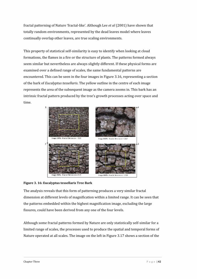
Chapter Three P a g e | 42
fractal patterning of Nature ‘fractal-like’. Although Lee et al (2001) have shown thattotally random environments, represented by the dead leaves model where leavescontinually overlap other leaves, are true scaling environments.This property of statistical self-similarity is easy to identify when looking at cloudformations, the flames in a fire or the structure of plants. The patterns formed alwaysseem similar but nevertheless are always slightly different. If these physical forms areexamined over a defined range of scales, the same fundamental patterns areencountered. This can be seen in the four images in Figure 3.16, representing a sectionof the bark of Eucalyptus tessellaris. The yellow outline in the centre of each imagerepresents the area of the subsequent image as the camera zooms in. This bark has anintrinsic fractal pattern produced by the tree’s growth processes acting over space andtime.
Figure 3. 16: Eucalyptus tessellaris Tree BarkThe analysis reveals that this form of patterning produces a very similar fractaldimension at different levels of magnification within a limited range. It can be seen thatthe patterns embedded within the highest magnification image, excluding the largefissures, could have been derived from any one of the four levels.Although some fractal patterns formed by Nature are only statistically self-similar for alimited range of scales, the processes used to produce the spatial and temporal forms ofNature operated at all scales. The image on the left in Figure 3.17 shows a section of the

Chapter Three P a g e | 43
gas clouds in the Eagle Nebula30, which is approximately 6500 light years away fromEarth. The height of the largest gas pillar on the left is approximately 4 light years, or 38x 1012 km. The image on the right shows some of the sandstone buttes within theMonument Valley, Arizona. The distance across this image is approximately 5km.
Figure 3. 17: Forms Produced by ErosionThe columns in the Eagle Nebula are formed from interstellar hydrogen gas and dustthat is gradually being eroded away by streams of ultraviolet light from nearby hot newstars―a process called photo-evaporation. The buttes in Monument Valley were formedwhen the soft shales in the area were eroded by rivers, which then exposed the hardersandstone.Although the forms in both images are on vastly different scales, they were producedby the same process―the process of erosion.Fractal DustAnother form of natural fractal patterning, described by Mandelbrot (1983, 210), is“Dust”. Like the Mandelbrot Set, Fractal Dusts, at higher magnifications, reveal moreand more of the same pattern. This effect is epitomised by the pattern of stars in thenight sky. If you look with the unaided eye you only one layer of stars. However, using atelescope some of the stars will resolve themselves into groups of stars. The further youmagnify the image, the greater the number of stars revealed. A typical telescopic starpattern is shown in Figure 3.18.
30 Image from the Hubble Telescope. NASA and the Space Telescope Science Institutehttp://hubblesite.org/newscenter/archive/releases/1995/44/image/a (accessed September22 2010)

Chapter Three P a g e | 44
Figure 3. 18: Star Cluster NGC 29031Fractal Dust patterns are simple to create with the toss of a coin. To begin the process, aselected area is divided into a basic grid pattern―here 3 x 3 (Figure 3.19). With the tossof a coin each successive grid square is selected to remain in or be removed from thepattern. The remaining selected grids are each subdivided into same grid pattern asbefore. The process is repeated until the limit of the required design resolution isreached.
Figure 3. 19: Fractal Dust
31 Image from the Hubble Telescope. NASA and the Space Telescope Science Institutehttp://www.hubblesite.org/gallery/album/entire/pr2006017c/warn/. Accessed 19 May 2011.

Chapter Three P a g e | 45
Fractal Patterning of Designed FormsPrior to the work of Mandelbrot describing fractal geometry, the use of fractalpatterning by humans in both art and architecture was unconscious and restricted tothe repetition of individual shapes at different scales; as seen in the floor tiling in theChurch of St Maria in Figure 3.10. This self-similar repetition can also be seen in ancientstructures such as gothic cathedrals (Lorenz 2002) and Hindu temples (Sala 2001).Interestingly, from the time of the Renaissance, a particular mathematical property wasused to try to explain both natural phenomena and also images in the arts. This was theGolden Ratio. It is now known that the Golden Ratio has fractal properties.The Golden Ratio, Art and ArchitectureSelf-similarity is reflected in the ‘Golden Ratio’, which has been known since the time ofEuclid (Livio 2002, 78). It is determined by the equation:
x2 = x + 1The positive solution to this quadratic equation gives the value of the Golden Ratio(Crilly 2007, 49), whereThis number is called Phi and as it has no finite solution is an irrational number32.The Golden Ratio is embedded within a sequence of numbers called the Fibonaccisequence by the French mathematician Edouard Lucas (1842―1891) in honour of theItalian mathematician Leonardo Fibonacci (1170s―1240s) (Livio 2002, 97). In thissequence, the first two numbers are 0 and 1, every other number in the sequence is thesum of the preceding two. Therefore, the sequence follows the pattern:
0, 1, 1, 2, 3, 5, 8, 13, 21, 34, 55, 89, 144, 233, 377, 610, 987, 1597...If a number in the sequence is divided by the preceding number (other then 0), theresults as shown below, rounded to six decimal places are achieved:1 ÷ 1 = 1.000000 55 ÷ 34 = 1.9617652 ÷ 1 = 2.000000 89 ÷ 55 = 1.6181823 ÷ 2 = 1.500000 144 ÷ 89 = 1.6179785 ÷ 3 = 1.666667 233 ÷ 144 = 1.61805632 An irrational number is one that cannot be expressed as a fraction.
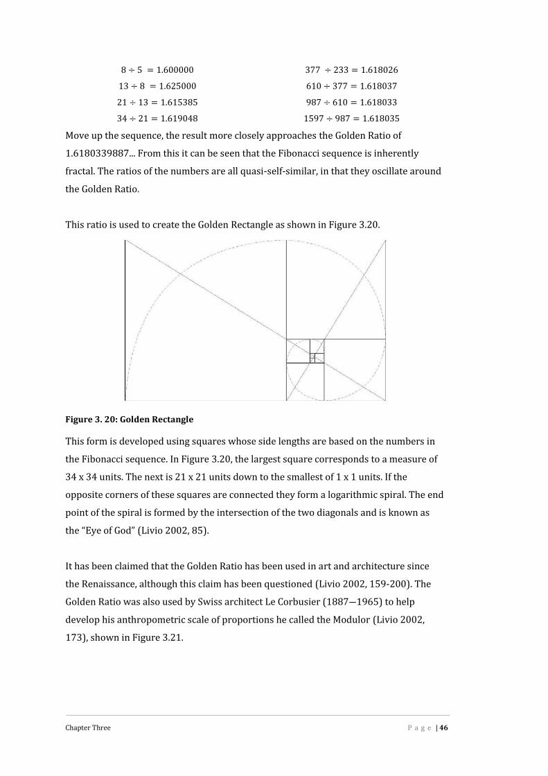
Chapter Three P a g e | 46
8 ÷ 5 = 1.600000 377 ÷ 233 = 1.61802613 ÷ 8 = 1.625000 610 ÷ 377 = 1.61803721 ÷ 13 = 1.615385 987 ÷ 610 = 1.61803334 ÷ 21 = 1.619048 1597 ÷ 987 = 1.618035Move up the sequence, the result more closely approaches the Golden Ratio of1.6180339887... From this it can be seen that the Fibonacci sequence is inherentlyfractal. The ratios of the numbers are all quasi-self-similar, in that they oscillate aroundthe Golden Ratio.This ratio is used to create the Golden Rectangle as shown in Figure 3.20.
Figure 3. 20: Golden RectangleThis form is developed using squares whose side lengths are based on the numbers inthe Fibonacci sequence. In Figure 3.20, the largest square corresponds to a measure of34 x 34 units. The next is 21 x 21 units down to the smallest of 1 x 1 units. If theopposite corners of these squares are connected they form a logarithmic spiral. The endpoint of the spiral is formed by the intersection of the two diagonals and is known asthe “Eye of God” (Livio 2002, 85).It has been claimed that the Golden Ratio has been used in art and architecture sincethe Renaissance, although this claim has been questioned (Livio 2002, 159-200). TheGolden Ratio was also used by Swiss architect Le Corbusier (1887―1965) to helpdevelop his anthropometric scale of proportions he called the Modulor (Livio 2002,173), shown in Figure 3.21.

Chapter Three P a g e | 47
Figure 3. 21: The Modulor33The Modulor was developed to provide “a harmonic measure to human scale,universally applicable to architecture and mechanics” (Livio 2002, 173).Architecture and Picturesque CompositionThe architectural forms of the Picturesque era have been examined by AndrewCrompton (2002). He argues that these traditional design forms have a lot in commonwith the fractal forms of Nature because the patterns produce by some elements withinthis design tradition obey a power law, which, has been shown to be the basis forfractal geometry. He defines architecture as fractal “…if it repeats and multiplies a form,such as a pointed arch, over several orders of size”.In his study on fractals and picturesque composition, Crompton re-interpreted some ofthe writings of John Ruskin (1818-1900). Ruskin had developed his aesthetics from astudy of nature, which “he equated with truth”. This empathy with natural forms wasevident in his drawing of a tree produced in 1858 (Crompton 2002, 458; Ruskin 1904).If Ruskin’s original drawing is compared with the image of a fractal tree subsequentlypublished by Mandelbrot (1983, 155), the similarities are obvious (Figure 3.22).
33 Image from: http://theory.ideacritik.com/?page_id=134, (Accessed May 5 2011)

Chapter Three P a g e | 48
Ruskin Tree-1858 Mandelbrot Tree-1977Figure 3. 22: Fractal Trees34Recently, the exterior forms of the buildings of Frank Lloyd Wright and Le Corbusierhave been analysed for their fractal properties (Lorenz 2009; Ostwald et al. 2008;Bovill 1996). It is interesting to note that the identified use of re-iterated forms atdifferent scales within these buildings is strikingly similar to the concept of ‘visualrichness’ proposed by Bentley et al (1985).The contemporary application of fractal geometry in architecture can be seen in thework of Frank Gehry. His design for the Guggenheim Museum in Bilbao used 26 petalsas part of a metallic flower. These were self-similar in form and were “unfolded, twistedand curved, generating a formal and spatial geometry” (Vyzantiadou et al. 2007, 52).However, one of the masterpieces of design based on the visual and structuralproperties of Natures forms and patterns is the Sagrada Familia basilica in Barcelona,Spain, by Antoni Gaudi (1852-1926). For example, Gaudi design for the main internalsupport columns is based on the branching structure of trees (Figure 3.23). Gaudi’s“belief in the beautiful efficiency of natural engineering clearly anticipated the modernscience of biomimetics35” (Berlin 2010, 22).Patterns of LandscapesAlthough there is no record of the conscious application of fractal patterning to largescale landscape development, retrospective analysis of forms at this scale has revealedsome interesting results. The work by Batty and Longley (1994) has shown that as wellas the boundaries of cities being complex fractal forms, the land use patterns withincities may also be fractal. This is supported by the fractal study of the urban form of TelAviv (Benguigui 2000). At the urban street level, Cooper et al (2010) have shown that34 Mandelbrot tree redrawn here for clarity35 For more information on Biomimetics see artisan 2009

Chapter Three P a g e | 49
the fractal dimension of certain types of urban street scenes have a positive associationwith perceived visual quality.
Figure 3. 23: Internal Support Structures for the Sagrada Familia36Analysing smaller scale forms, Andrew Crompton (2001) examined how space wasused by adults and children. He proposed a new measure for space based on thenumber of “places”, within a space, that were suitable for activity. Using this, he foundthat spaces which contained more places for activities had a higher fractal dimensionthan those that contained less. He extrapolated this finding and proposed that currentresidential housing densities did not take into account the “plastic possibilities ofspace” and suggests that if they were designed to have higher fractal dimensions, basedon potential activity level rather than physical size, they might enable the creation ofresidential areas which could accommodate more “places”.This area of analysis has been extended by Chen and Zhou (2008) who found that thescaling laws (level of complexity) of urban systems are analogous to those of riverssystems and by Thomas el al (2009) who analysed the variation in the spatialarrangement of buildings at the regional level. Thomas et al (2009, Section 59) conclude36 Image: http://commons.wikimedia.org/wiki/Commons:Reusing_content_outside_Wikimedia.Accessed 27 January 2012

Chapter Three P a g e | 50
that a fractal approach to analysing urban patterns, “helps us to improve ourknowledge of their spatial organisation, regardless of how planned they were”.Similarly, Pierre Frankhauser (2008) suggests that a fractal approach to developingurban patterns is an important spatial goal.The techniques of fractal geometry have also been used to analyse natural objects,textures and pictorial scenes (Ruderman 1994; Ruderman and Bialek 1994; Taylor2002) and various types of landscapes from an aerial perspective (Xu et al. 1993).Other research has shown that human discrimination of images is higher for imageswith a fractal dimension similar to that of natural terrain surfaces (Knill et al. 1990). Ithas also been proposed that humans prefer images with a one-dimensional fractaldimension in the mid-range from 1.3 to 1.537 (Spehar et al. 2003). However, it seemsthat the unconscious use of fractal patterning may play a role in the aesthetic responseevoked by some designed landscapes.The Ryoan-ji Temple GardenResearch by Gert van Tonder and Michael Lyons has shown that fractal patterning isembedded within the dry landscape garden of the Ryoan-ji Temple in Japan (Tonderand Lyons 2005) . Using a technique known as medial-axis transformation38, they haveshown that the overall structure of this dry garden is based on a spatial form similar tothat of a branching tree. They determined that the connectivity pattern of the branchesis self-similar and the trunk of the tree form converges on the main viewing area for thegarden. By changing39 either the placement or the number of rocks within the garden,they found that the self-similar tree form and convergence on the main viewing areawas removed from the corresponding medial axis. From this analysis, they concludedthat the structure defined by the negative space was not accidental and that the ancientdesigners of these sophisticated, minimalist gardens may have had an intuitiveunderstanding of the patterns of Nature. In their discussion, they suggest that theirwork uncovers a new link between the structure of the Ryoan-ji Temple garden and itsaesthetic appreciation ― a link based on the self-similar structure of the garden.
37 This measure is based on the one-dimensional analysis of fractal lines rather than a 2-dimesional analysis of fractal planes as discussed in Chapter 6.38 The medial-axis transformation is a method for representing the shape of objects by findingtheir topological skeleton.39 This was achieved by digital manipulation of photographs

Chapter Three P a g e | 51
Patterns of ArtSimilar to the analysis of urban form, fractal patterning and self-similar repeated forms,at different scales, have been discovered within various artistic compositionaltechniques. This has been recognised in both Eastern and Western art. Two examplesof this are discussed.John Briggs (1991) proposed the term ‘reflectaphor’ to refer to repeated forms, whichhe suggests perform the same function, in visual terms, as the language basedmetaphor . He also attributes the potential ‘deep sense of coherence’ in a piece of art tothe presence of these reflected forms. He demonstrated this concept through theanalysis of an old Chinese painting, shown in Figure 3.24a below. Here, thereflectaphors occur among the ‘shapes, colours and lines’ of the painting. Briggsidentifies a triangle shape with a dot at the apex as the root reflectaphor, based on theshape of the umbrella in the painting. He identifies other areas within the paintingwhere this shape is ‘reflected’. These are shown in Figure 3.24b highlighted in white,with some additional ‘reflectaphors’ identified.
Figure 3. 24: Man With Umbrella40Although these shapes are not identical, they have similar properties to the root shape.As Briggs explains:Each [triangle shape] is reflectaphorically both there and not there since eachfigure's lines are also lines of other triangles, other parts of the composition.Thus, while the this* other-ness spreads an implicit recognition of the40 Permission to use this image has been granted by John Briggs

Chapter Three P a g e | 52
[triangle shape] everywhere, it keeps its distance so the similarities are neveroverstressed or conclusive.Similarly, Taylor et al (1999; 2002; 2005) have shown that Jackson Pollock’s ‘drip andsplash’ technique of expressionistic composition produced highly fractal paintings.Using the one-dimensional Box-Counting method41 they demonstrated that Pollockgradually increased the fractal dimension of his paintings over the years from 1945 to1952 from a level close to one, to a maximum of 1.72. They have also speculated that asPollock’s technique matured, he intuitively tried to achieve paintings with a fractaldimension of around 1.7. Using the two-dimensional fractal analysis techniquedeveloped for this research42, Pollock’s painting Blue Poles Number II, painted in 1952and shown in Figure 3.25, has been analysed. The resultant fractal dimension of 2.78aligns quite well with the result obtained by Taylor et al and their one-dimensionalmethod.
Figure 3. 25: Jackson Pollock Blue Poles 1952 National Gallery of Australia, Canberra,purchased 1973 © Pollock-Krasner Foundation43
ConclusionAlthough fractal geometry can be used retrospectively to analyse the complex patternsof Nature, it is clear from the discussion above that unlike Euclidean and Cartesiangeometries, the application of fractal geometry to landscape design is undefined. Thereasons for this are clear; with Euclidean geometry it is a simple process to design awall 1200mm high, 200mm wide and 10m long and there is only one solution.However, the patterns and forms described by fractal geometry are the result of non-linear, re-iterated processes—either deterministic, as in the exact self-similar form ofpure mathematical processes, or stochastic as in the forms produced by Nature. Unlike41 This is discussed in Chapter 6.42 This is discussed in Chapter 643 Copyright permission granted from the National Gallery of Australia
Chapter Three P a g e | 53
the deterministic patterns produced by pure mathematical processes, the stochasticprocesses of Nature make the final form almost impossible to predict.However, what is meant by Nature or natural processes is an ongoing philosophicaldebate that in the West revolves around the conception of a Nature―culture duality.The concept of Nature and its relationship to human activity is the focus of the nextchapter.
Chapter Four P a g e | 54
Chapter Four
nature or Nature
I wish to speak a word for Nature, for the absolute freedom and wildness,as contrasted with a freedom and culture merely civil, ― to regard man
as an inhabitant, or a part and parcel of Nature, rather than a member ofsociety. (Thoreau 1991, 71)
IntroductionAs discussed in Chapter 2, one of the major metaphysical, political, and culturalprograms facing landscape design44 today is the concept of ecologically sustainabledesign. The core issue within this is the human relationship to the non-humanenvironment; often referred to as the Nature―culture duality.The importance to landscape design of the relationship between human culture andnature is evident when Catherin Bull (1996, 27), argued that the content of landscapedesign is nature. However, landscape design is an intentional human action andtherefore must be considered a reflection of its culture (Rogers 2001, 59). Similarly, asignificant part of the content of a designed landscape comes from human artefacts,such as concrete, steel, glass and plastic. Therefore, the word nature, as used here,could be interpreted as being all encompassing ― everything is nature. The counterargument to this is provided by postmodern philosophy, that considers nature as acultural construct and the human species as separate from nature (Hay 2002, p1-25).However, given that language is a symbolic representation of something, it is thatsomething, in this case nature, that requires greater definition. This is analogous towhat Fred Dretske (1999) describes as distinguishing between object perception andfact perception, and that which Sorvig (2002, 10) describes as separating “nature-the-concept from nature-the phenomena”. Therefore, how the relationship between natureand culture is understood is very important as it has a direct impact on the physicalform of designed landscapes (Sorvig 2002, 9) and their potential impact on the widerenvironment. This argument is implicit in Treib’s (2002, 121) proposition that“...landscape design―consciously or not―always reflects contemporary values andattitudes” and explicit when, as noted by Jennings (2010, 22), “the biggest single reason44 The term landscape design is used here to signify the creative process that “intentionallyredirects or reorganizes energy and materials” (Musacchio, L. R. 2009)
Chapter Four P a g e | 55
why plants and animals are endangered is because habitats are being destroyed orpolluted.”Given this, there can be little doubt that our Western attitudes towards nature have aprofound effect upon the development of sustainable landscape forms. Therefore, forthe purposes of this research it was necessary for the author to reach a clearerunderstanding of what is meant by the term Nature. This was considered essential inorder to understand the potential use of fractal geometry, described as the geometry ofNature, within design.As the author is a product of Western Culture and the Judeo Christian religion, thischapter examines some of the philosophical roots of our Western attitudes towardsNature and develops a new understanding that enables a more objective way torecognise Nature and what it is natural within the context of this research.Nature the WordAs Sorvig (2002, 4) correctly points out, the confusion over the meaning of the wordNature is not the fault of any one profession. The word Nature has been used over timeto refer to many different aspects of human and non-human life. The Oxford English
Dictionary (OED) currently lists 27 definitions of Nature that fall within six overarchingcategories. These are:1. Senses relating to physical or bodily power, strength, or substance2. Senses relating to mental or physical impulses and requirements3. Senses relating to innate character4. Senses relating to the material world5. Phrases6. CompoundsThe current confusion over the meaning of this word is epitomised by the followingdefinitions from the OED included under category 4 above:11a: The phenomena of the physical world collectively; especially plants,animals, and other features and products of the earth itself, as opposed tohumans and human creations.11b. In wider sense: the whole natural world, including human beings; thecosmos.
Chapter Four P a g e | 56
Definition 11a implies that humans and human creations are not phenomena of thephysical world. Similarly, the OED marks definition 11b, which includes humans as partof the natural world as obsolete. This implies that the human species is unnatural!In contrast the Queensland Nature Conservation Act of 1992, defines nature as:1. “Nature” includes all aspects of nature.2. Without limiting subsection (1), “nature” includes―a. ecosystems and their constituent parts; andb. all natural and physical resources; andc. natural dynamic processes; andd. the characteristics of places, however large or small, that contribute to―i. their biological diversity and integrity; orii. their intrinsic or scientific value.In this definition, Nature and nature seem to be the same thing. However, Nature couldbe interpreted to mean either the OED definition 11a or 11b depending on whetherhumanity is considered an aspect of Nature by the interpreter of the statement. What isclear from the OED is that our understanding of Nature changes over time.Pre-Industrial NatureIn her book, The Death of Nature, Carolyn Merchant has argued that pre-industrialpeople had a more organic, mystical and symbiotic relationship with the rest of theirenvironment than do people today (Merchant 1982, p1-41). Although there is noabsolute way of knowing how our early human ancestors conceptualised theirenvironment, there can be no doubt that they were much closer to a nature thatdirectly provided the means for them to survive.Hay (Hay 2002, 11-13) has indicated that through history there are two main themeswith respect to human’s relationship with what he calls wilderness45. One theme is thatadopted by the Romantics and is a wilderness of the pastoral paradise where “..such a‘paradise’ is not really wilderness. It is leached of its ‘wild-ness’; it is a nature tamed,not wild nature”. The other theme is that wilderness was a place to be feared. There canbe no doubt that for pre-industrial people the most significant fact in their lives wassurvival and at this time, the wild forests contained very real physical dangers such as45 Although wilderness is not clearly defined it is implied to mean areas untouched by humanactions.

Chapter Four P a g e | 57
wolves and bears and other dangerous humans. The wild forests were also the sourceof culturally perceived dangers such as supernatural entities. This aspect of wildernessor ‘wild nature’ can also be discerned in folklore and nursery tales where woodlandsand forests are often described as dark, evil places to be avoided, especially at nightwhen they are full of goblins, witches, trolls and other sinister creatures that will trapthe unwary.This aspect of Nature is implicit in the definition of wilderness in the OED and also inthe Judeo-Christian tradition. In both the Old and New Testaments of the King James
Bible there are many references to ‘wilderness’ but in general these reflect a place thatis to be avoided.Regardless of how wild-nature is conceptualised, Hay (Hay 2002, 12) has correctlynoted that:... the history of human civilisation can be seen as a history of escaping fromwilderness; of establishing mastery over it through fire, clearing, cropping,domestication of animals, and so on.This argument is also supported by Keith Thomas (Thomas 1984, 25-30).There can be little doubt that the majority of Western people still manifest this innatedichotomy with respect to wild-nature. This fear is implicit when Marc Treib (1999, 39)discusses his preference for Nature as found in a garden, which “...represents theconfluence of natural processes with human intelligence and sensibilities”. However, inthis statement Treib not only manifest an implicit fear of wild-nature, but implies thatnatural processes are separate from human processes. This perceived split betweenhumanity and Nature is also considered an outcome of both theology (Hendry 1980;Thompson 2003; White 1967) and philosophy (Audi 1999; Robinson and Groves 1998;Hendry 1980).If, as Bertrand Russell (1959, 159) suggested, philosophy is central to enlarging “...ourconception of what is possible”, its roots to our ideas of Nature must be examined. Inthis respect, two of the most important philosophers that have changed Westernthought with respect to humanity and Nature are René Descartes (1596-1650) andBenedict Spinoza (1632-1677).
Chapter Four P a g e | 58
Humanity, Nature and Two Metaphysical Positions
René Descartes (1596-1650) was a French mathematician and is considered to be thefounder of modern scientific thinking and Western philosophy (Cottingham 1999). Hisbelief in the dominance of mind over physical matter is epitomised by his famousexpression “cogito ergo sum”, or ‘I think therefore I am’. Descartes reached hisphilosophical conclusion through the application of a methodology called systematicdoubt, which emphasised the difference between thinking and perceiving (Robinsonand Groves 1998, 54). To Descartes all perception was questionable. The only thing hecould not doubt was the fact that he was thinking. Descartes’ philosophy dividedexistence into two totally separate arenas ― the mental and the physical. Descartes sawthe physical body as a machine; its purpose was to provide a vehicle for the mind.Although his mind-body dualism is now considered to be problematic, he raisedquestions with regard to the human mind and its relationship to the physical world thatare still far from being resolved. It is this dualism between mind and body, spiritual andphysical that underlies the dichotomy between humans as thinking beings and humansas part of a spatiotemporal physical environment that Cottingham (2001) describes asa “philosophical-cum-scientific puzzle of enormous importance...”.Benedict Spinoza (1632-1677) was one of Holland’s most important philosophers andis regarded as one of the 17th century’s most important rationalist thinkers (Garrett1999). Although he studied Descartes, he is thought to have come nearer to the truththan any other philosopher who has addressed the same imponderable metaphysicalquestions of life46, and his work is still considered to be of major importance tophilosophical thinking today (Scruton 2001, 138-139).Spinoza rejected Descartes’ dualism and considered existence as being composed oftwo forms of entities: those that are dependent on other entities, and those that areindependent. For example, the author’s existence would be seen as being dependentupon the existence of the author’s parents, whose existence was dependent upon theirparents, and so on ― a chain of dependencies. For Spinoza, the only independent entitywas God; all other entities were lesser modes of this one independent entity. At theheart of his metaphysics Spinoza’s identifies God with Nature (Garrett 1999, 870). In46 These questions are: Why does anything exist? How is the world composed? What are we inthe scheme of things? Are we free? How should we live? (Garrett 1999)

Chapter Four P a g e | 59
some sense, Spinoza’s concept of God can be considered to be equal to an allencompassing concept of Nature, where all entities in existence are considered asconstituent parts. Thus, in some ways, his metaphysics can be understood as Naturebeing the entity from which all other entities depend (Scruton 2001).Spinoza viewed the mind-body duality of Descartes as being two ways of expressingthese modes of existence within the single entity God or Nature. Brought down to thehuman level, Spinoza saw the mind and body as being two separate instances of thesame entity, rather than two completely different entities (Scruton 2001)―like the twosides of the same coin. Thus, unlike Descartes’ dualism, Spinoza’s metaphysics is a formof monism47 (Mclaughlin 1999, 686). However, this position is considered anti-humanist48 as it sees humanity as the result of a form of extreme determinism49 with nofree will (Eagleton 1996, 129).Postmodernism has rejected this view and argues that reality cannot be separated fromthe way it is represented by language (Ward 1997, 89). This can be understood byexamining the quote from Romeo and Juliet below:‘Tis but thy name that is my enemy;Thou art thyself, though not a Montague.What’s Montague? It is not hand, nor foot,Nor arm, nor face, nor any other partBelonging to a man. O, be some other name!What’s in a name? That which we call a roseBy any other name would smell as sweet;So Romeo would, were he not Romeo call’dRetain that dear perfection which he owesWithout that title. Romeo, doff thy name,And for thy name which is no part of theeTake all myself.(Shakespeare, Romeo and Juliet Act II, Scene II)Here, Shakespeare has managed to express the beauty, power and complexity oflanguage as a means of communication. Language is a symbolic system, where the wordsymbols have meaning(s) given to them by the users of that system (O'Neil 2006). Whatis relevant in the quote above is the word-symbol ‘Montague’. To Juliet and herextended family the word-symbol ‘Montague’ and the material form it represents are47 Monism sees all reality as being of one kind.48 Humanism is a philosophical position that recognises human beings have unique “capacitiesand abilities” that should be celebrated and cultivated through education for their own sake.(Kolenda 1999)49 Determinism is the view that the current state of an entity is dependent on its antecedentstates “in accordance with universal causal laws that govern the world” (Berofsky 1999).

Chapter Four P a g e | 60
congruent and mean ‘enemy’. To Romeo and his extended family it means ‘friend’.However, when Juliet falls in love with Romeo, as a physical being, she tries to separatethe meaning of the word-symbol from the meaning of the material form it applies to; itis not the ‘man’ who is now her ‘enemy’, but the word-symbol. With another word-symbol applied to the material form, the ‘man’ would not be thought of as ‘enemy’, butcould be thought of as ‘friend’ while still retaining all the same material form. Here,Shakespeare, through Juliet, tries to construct a new reality through the use oflanguage.This dichotomy between the meaning(s) of a word-symbol and the material form itrepresents are clearly evident in the field of landscape design. When discussingecology, James Corner (1997, 84) states that “Ecology constructs particular ‘ideas’ inthe imagination of its advocates; it conjures up particular ways of seeing and relating toNature...”. He therefore describes the need for two natures. Firstly ‘nature’, which heproposes is a referent for people’s ideas and understandings of the natural world andhow they communicate them. Secondly he describes a capitalised Nature as a referentfor the physical reality that is the total cosmos, which he states “exceeds humanunderstanding”. This argument is echoed by Hay (2002, 24) who states that withinenvironmental thought, “few people, within the field of environmentalism, havedifficulty with the real world/social construct divide”.Emily Brady (1998, 52-53) expands on this when she notes that there are two opposingviews. The first is where Nature is considered as real and humans are just a part ofNature; this she calls the “nature endorsing” view that reflects a holistic environmentalposition. The second is where Nature is considered just a cultural construction andeverything is cultural; this she calls the “nature-sceptical” view and argues that thisview is rooted within Postmodern theory. Hay (2002, 20-22) supports this argumentwhen he considers that the claim “nature is a social construction” is due to bothMarxism and Postmodern deconstructionism.Although there is no doubt that most people would accept the ontological existence ofthe physical reality that is called Nature (Barry 1994, 391; Treib 2002, 121; Hay 2002,22). Trieb’s (2002, 121) comment that “there is no concept of nature free from aconcept of culture” implies that one cannot exist without the other.
Chapter Four P a g e | 61
It could be argued that we have come full circle, where the Postmodern view of Natureand culture reflects Descartes’ mind-body dualism and the new environmental viewreflects Spinoza’s monism. Sorvig (2002, 9) argues that the “culture as separate fromnature”, the “nature as extension of culture” and the “culture is a part of nature” viewsare all obstructive to critical thought on how human activities “differ from the rest ofwhat goes on here on Earth”. Therefore, in terms of sustainability, it seems essential todevelop a new framework that enables discussion about Nature, about what constitutesnatural and how humanity fits into this overall picture. To this end Trieb (2002, 131)provides a clue when he says “Could we not regard landscape design as giving form tonatural processes constrained by contemporary social and aesthetic conditions,executed in a mere blink in geological time.” This is supported by Brady (Brady 2003,53) when she argues that ‘Nature is not subsumed by culture’. By understandingNature’s processes we can examine how Nature is affected by culture and wherehumanity is positioned within it.The Nature―culture arguments are also reflected in how the separation betweenhuman and non-human are defined. The word natural is normally only applied to thenon-human world whereas unnatural is normally applied to all human artefacts andprocesses, but interestingly not to ourselves. How, therefore, can we distinguishbetween ‘human’ and ‘non-human’ within the world we experience? John Barry (1994,391) suggests a way forward when he says: “...the environment unlike ‘nature’ canencompass both human and non-human aspects of what we often mean by‘environment’.”Both natural processes and environments form part of the field of Ecology.Ecology and NatureEcology is the study of the relationships between living organisms and theirenvironment. Within ecology, the concept of an ‘environment’ defines the total physicalsurroundings within which an organism operates. The environment is sub-divided intotwo parts: the biotic component, which consists of all living organisms and the abioticcomponent, which consists of the non-organic parts of the earth as well as non-organicprocesses including, the weather (Cotgreave and Forseth 2002, 3; Jennings 2010, 3).The beauty of the concept of an environment is its spatial and temporal scalability. Forexample, at the spatial level a human environment can be defined as the whole Earth, a

Chapter Four P a g e | 62
city or just a small room. At the temporal level, individual organisms can only beaffected by things within their own lifetime; however, whole species of organisms canbe affected by processes over a wide range of time scales. As Cotgreave and Forsythe(2002, p14-17) note, science tells us that the natural process of evolution has beenongoing for the last 3.5 billion years, whereas human evolution is thought to havebegun seven million years ago (Kemmer 2008) ― a ratio of 1:5000.Environmental ProcessesAlthough there are many abiotic and biotic cycles, there are two fundamental processeswithin ecology that are essential for life on earth to be maintained. These processes arethe food chain and the hydrological cycle (Jennings 2010, 11; Cotgreave and Forseth2002, 204). The food chain is the chain of energy that passes from one living organismto another. All living organisms require some form of food to produce energy to live.Energy is required to grow, keep the correct temperature and reproduce. The vastmajority of food chains begin with plant life that converts sunlight to energy throughthe process of photosynthesis. Plants are then eaten by herbivores, which in turn areeaten by carnivores. Some species, such as humans, eat both plants and other animals.Except for some deep sea ecosystems that use geothermal energy as their energysource (Roberts et al. 2005), the primary energy source for all ecosystems on Earth isthe Sun. The hydrological cycle involves the evaporation of water from the world’soceans, rivers and streams into the atmosphere, which then falls as rain back onto theland. This cycle is also driven by the sun.Recognition that the Sun, gravity and in a small way Geo-thermal energy, are the onlysources of energy that drive natural processes, provides a platform for a newframework for looking at the concept of Nature and natural, as it is clear that one of theprimary differences between the human organism and other organisms is that thehuman organism uses energy for discretionary purposes other than organicmetabolism. This is evident in the Brundtland Report and current discourse on globalwarming due to the fossil fuels we burn to power, for example, automobiles, aircraft,computers and televisions.A New Framework for Understanding NatureDesign is a complex term that can be either a verb or a noun. As stated previously, inthe context of this study, design is defined as a creative process that intentionallyredirects or reorganises energy and materials. Therefore, from an ecological

Chapter Four P a g e | 63
perspective, design is just another way that the human organism interacts with itsenvironment. However, the concept of ‘human intention’ associates the form of adesigned landscape to the human culture that created it.Environment and LandscapeIt has been argued that the concept of a ‘landscape’, as distinct from that of an‘environment’, is a product of the early Enlightenment period during the 16th century,underpinned by the mind-body dualistic philosophy of René Descartes discussed aboveand Issac Newton’s (1643―1727) theories of absolute space and absolute time (Fungand Jackson 1996, 2). However, the difficulty in defining landscape is highlighted by theAustralian Institute of Landscape Architects in their ‘Australian Landscape Charter’(AILA 2009, 7), wherein they define landscape as: “...those landscapes that are: Urbanand Regional; Rural and Natural; Modified and Unmodified”.Using the word landscapes in the definition of landscape is a nice circular definitionthat does not provide much insight into what a landscape actually is. This complexityand plasticity has been well documented by others50. In contrast, Simon Swaffield(2002, 5) conceives landscape as either a “symbolic system” or as a system for:“...healthy, functional and pleasurable places for people and communities to whichsignificance and meaning will accrue over time.” As noted above, (1996, 27) arguesthat the content of a designed landscape is “nature”, therefore the content of a designedlandscape cannot be separated from cultural attitudes towards nature. Marc Trieb(2002, 121) argues that the content of designed landscape can be:...gauged along three axes: the formal (which includes space, form, andmaterials); the cultural (which includes history, social mores, and behaviour);and the environmental (among them ecology, topography, hydrology,horticulture and natural process).Treib’s proposition that environmental processes form one axis within the ‘content’ of adesigned landscape relates to the environmental processes discussed above.Recognising that a designed landscape is a combination of structural form, humanculture and environmental processes and combining this with the realisation that theuse of discretionary energy can differentiate between human and non-human activitiesand processes, provides a framework for the development of a new understanding ofthe concepts of Nature and natural. This framework is shown in Figure 4.1.50 See for example: Jackson 1984, Palka 1995, Dennis 2002

Chapter Four P a g e | 64
Like Spinoza and Berleant (1992, 8-9), this framework recognises that themetaphysical reality of Nature is all encompassing and that human culture is part of anoverall Nature. However, it distinguished between two types of Nature, Wild Natureand Designed Nature. These two natures are differentiated by three parameters; theway energy is obtained, the processes used to create structural form and theintentional actions based on human culture.
Figure 4. 1: Nature Re-framed
What is also clear from Figure 4.1 is that through our perception and derived meaningof Natural and Para-natural environments, we modify Nature according to our culturalrequirements. This in turn modifies our perception and derived meaning of theseenvironments.

Chapter Four P a g e | 65
Wild NatureWild Nature is responsible for the creation of Natural environments. Theseenvironments are formed through the input of primary energy, the action of Naturalprocesses and the creation of Natural elements. Primary energy is energy sourceddirectly from the Sun, geo-thermal activity or gravity. Nuclear fission is also included inthis list as there are clear indications that a naturally occurring nuclear fission reactorexisted in Gabon, West Africa, about 1.7 to 1.9 billion years ago (Cowan 1976; Karam2005). However, as the author is unaware of any Natural processes or life forms thatdepend on this energy it is only shown in small print in Figure 4.1.This framework also recognises that some natural entities require the energy derivedfrom the burning of timber for their propagation and regeneration. However, fire isconsidered a minor primary energy source in the production of Natural environments.Designed NatureDesigned Nature is responsible for what are here called Para-natural environments.The term Para-natural is used as a rejection to the negative concepts inherent in theterm unnatural. Para originates from the Greek and is used to denote things in thesense of “analogous or parallel to, but separate from or going beyond, what is denotedby the root word” (OED 2010). This seems a very appropriate term to describeenvironments that have been modified or created by human culture as these go beyondwhat can be expected from Natural-environments. The term Para-natural is also non-judgemental.Para-natural environments are formed through the input of both primary andsecondary energy, where secondary energy is created through burning timber, coal, oilor gas. Secondary energy is also created through nuclear fission. Although not shown inFigure 4.1, electricity created from the capture of solar, wind, tidal or geo-thermalenergy is also considered as secondary energy as it requires an interface for itsproduction. The combination of primary and secondary energies, Natural and humanprocesses and Natural and human elements form Para-natural environments.Designed EnvironmentsThe vast majority of environments that humans interact with are, by definition, Para-natural, even though many of these environments include the same elements andprocesses found in Natural environments, such as biological growth, the food chain and

Chapter Four P a g e | 66
the hydrologic cycle. The ratio between the primary and secondary energy and theratio between Natural and human processes required to create and support Para-natural environments will fall on a sliding scale that ranges from primary and Naturalat one end to secondary and Human at the other. All designed environments will fallsomewhere between the two. However, it may be asked, given the proliferation of thehuman species, do Natural environments exist? Brady (2003, 53) has argued that“While nature may be thought of as that which is untouched by us, in actuality, much ofit is modified in varying degrees by agriculture, humans living in the land, and the builtenvironment of towns and cities.”.If Natural environments are considered the embodiment of ecological sustainability, asthey surely must be, then for a designed environment to be ecologically sustainable (interms of energy) they must trend towards being supported predominantly by Naturalprocesses driven by primary energy.NatureWild Nature on Earth has evolved over time periods that extend far beyond the normalhuman range of conception. It has evolved via an almost infinite number of complexand dynamic interrelated processes and events, over the course of geological history.These dynamic, non-linear processes have generated a world full of self-similarpatterns of incredible intricacy, whilst maintaining a seemingly inherent order andsimplicity. These patterns cannot be described by Euclidean or Cartesian geometry, butthey are capable of being described by fractal geometry.It has taken around 18,000 years for Wild Nature to evolve from the last Ice age to itspresent state. However, over the last 200 years the rapid growth of Para-naturalenvironments has put pressure on this evolution to the point in which discontinuousand radical change is now a real possibility. However, as both ecology andpalaeontology teach us, Wild Nature has no difficulty with radical discontinuities. Therecovery of the Victorian mountain ash forests after the devastating bushfires ofFebruary 2009 (Gilmour 2011) has been well documented.Furthermore, the five global mass extinctions that are known to have occurred overgeological time caused significant mass extinctions (Robinson 2006). This is shown inTable 4.1.

Chapter Four P a g e | 67
Table 4. 1: Mass Extinctions
Period mya51 Percentage of Species ExtinctOrdovician-Silurian 435 85Late Devonian 370 82Permian-Triassic 240 96End Triassic 205 76Cretaceous-Tertiary 65 76(Summarised from Robinson 2006)Although Robinson (2006) has estimated that if the human impact on global ecosystemis not addressed then by 2050, 50% of all species may be either endangered or extinct.However, it could be argued that without the past extinction events the human speciesmay not have evolved.Globally, the underlying rationale for ecological design is to limit the impact of Para-natural environments on Natural environments, so that together they continue tosupport human life. The principles of sustainability, based on the UNWCED (1987)report, have become synonymous with ‘good’ design for all disciplines in the builtenvironment arena. But the concept of sustainability is meaningless unless it is in atemporal context. The UNWCED expresses this context as intergenerational equity. Butover how many generations can we assess the impact of our actions? Chaos Theory, asportrayed by the ‘butterfly effect’, predicts that we can never foresee all of theoutcomes, over time, of any one action. Clearly, the interplay of systems within thisworld are too complex to describe.How we conceive and understand Nature is very important. This exemplified by the therecent project to re-establish pre-European settlement prairie lands in Chicago, USA.Re-establishment of these prairie lands would have involved large-scale tree clearingand as such have caused major conflict between community members over just who’sconcept of ‘nature’ should be recognised—‘Nature as was’ or ‘Nature as is’. So thequestion, ‘for how long do we want a landscape to be sustainable?’ is valid. Butextended and geological time periods are meaningless to people who may think only interms of a few generations. It could be argued that the guiding principle should be, ‘isthis landscape natural enough‘, rather than ‘is this landscape sustainable’. However, theprocesses of Wild Nature alone do not guarantee the survival of any species. But, theyare essential to the survival of all species. The recent earthquakes in New Zealand andJapan are testimony to the destructive power of Wild Nature.51 mya: millon years ago
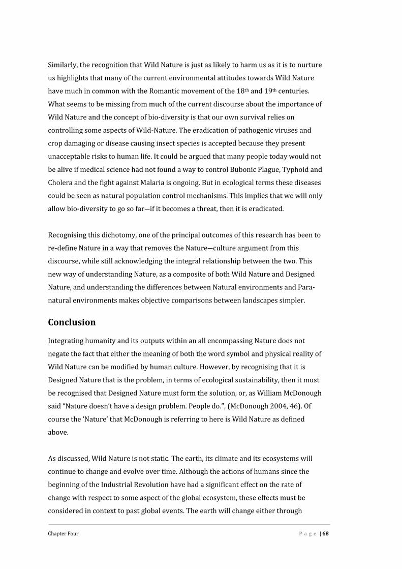
Chapter Four P a g e | 68
Similarly, the recognition that Wild Nature is just as likely to harm us as it is to nurtureus highlights that many of the current environmental attitudes towards Wild Naturehave much in common with the Romantic movement of the 18th and 19th centuries.What seems to be missing from much of the current discourse about the importance ofWild Nature and the concept of bio-diversity is that our own survival relies oncontrolling some aspects of Wild-Nature. The eradication of pathogenic viruses andcrop damaging or disease causing insect species is accepted because they presentunacceptable risks to human life. It could be argued that many people today would notbe alive if medical science had not found a way to control Bubonic Plague, Typhoid andCholera and the fight against Malaria is ongoing. But in ecological terms these diseasescould be seen as natural population control mechanisms. This implies that we will onlyallow bio-diversity to go so far―if it becomes a threat, then it is eradicated.Recognising this dichotomy, one of the principal outcomes of this research has been tore-define Nature in a way that removes the Nature―culture argument from thisdiscourse, while still acknowledging the integral relationship between the two. Thisnew way of understanding Nature, as a composite of both Wild Nature and DesignedNature, and understanding the differences between Natural environments and Para-natural environments makes objective comparisons between landscapes simpler.ConclusionIntegrating humanity and its outputs within an all encompassing Nature does notnegate the fact that either the meaning of both the word symbol and physical reality ofWild Nature can be modified by human culture. However, by recognising that it isDesigned Nature that is the problem, in terms of ecological sustainability, then it mustbe recognised that Designed Nature must form the solution, or, as William McDonoughsaid “Nature doesn’t have a design problem. People do.”, (McDonough 2004, 46). Ofcourse the ‘Nature’ that McDonough is referring to here is Wild Nature as definedabove.As discussed, Wild Nature is not static. The earth, its climate and its ecosystems willcontinue to change and evolve over time. Although the actions of humans since thebeginning of the Industrial Revolution have had a significant effect on the rate ofchange with respect to some aspect of the global ecosystem, these effects must beconsidered in context to past global events. The earth will change either through

Chapter Four P a g e | 69
human action or through the actions of Wild Nature. Therefore the key to long termsustainability is to ensure that Natural and Para-natural environments becomemutually self-supportingThe new framework for Nature, illustrated in Figure 4.1, proposes two Natures existingin parallel but in a symbiotic relationship to each other. It recognises that DesignedNature is dependent on Wild Nature and also that Designed Nature can have asignificant impact on Wild Nature. It also recognises that Nature is all encompassingand that human culture is part of that overall Nature. However, a key aspect of thisframework is that it recognises Nature is itself a recursive entity. This recursion isimplicit in the comment from Trieb (2002, 121); that there cannot be a concept of“nature” free from a concept of culture. However the corollary of this statement is thatthere cannot be a concept of culture free from a concept of Nature.We cannot understand ourselves without understanding Nature, but to understandNature we have to understand ourselves. This recursion explains why the discourse onNature is so confusing and vague and why the Nature―culture debate cannot beresolved. It also mirrors the knowledge that the known universe as well as manycultural patterns and processes are based on recursive structures. However, anyrecursive process requires building blocks on which the process of recursion operates.Within the domain of landscape architecture Trieb’s paper identifies some of thesebuilding blocks as: Form, Process and Culture and it is these building blocks that echoin the frameworks previously discussed in Chapter 2.Within this thesis, the building block of culture is expressed through the philosophicalconcept of aesthetics. The next chapter discusses the concept of aesthetics and itsimportance to design.

Chapter Five P a g e | 70
Chapter Five
Aesthetics
It is critically important to understand that landscape is two things at once; a
collection of material objects within a scene and the ideas that make those
objects meaningful. (Dennis 2002, 26).
IntroductionA common theme in the frameworks discussed in Chapter 2 is the complex interactionbetween human culture, nature52 and the aesthetics of designed landscapes. Withinmany discussions, the term aesthetics is used as if it applies only to the overall physicalform of a landscape ― synonymous with the term style. But it is clear from thephilosophy of aesthetics that aesthetics also involves a human mental response that hasmultiple components. To say that ‘something’ has a particlualr aesthetic, implies that itis possible to predict the human emotional and cognitive response to that ‘something’.This becomes even more problematic in a multi-cultural society such as Australia.The power of aesthetics to influence how we perceive the world around us has beenrecognised by aestheticians, designers and psychologists (Nassauer 1997a; Richards2001; Eaton 1997). Similarly, over the last few years, an awareness of the importanceof aesthetics to designed landscapes has been growing. As discussed in Chapter 2, thishas been reflected in the call for a move towards a new design aesthetic for our“ecological age”. However, like the concept of Nature, discussed in Chapter 4, the term‘ecological aesthetic’ has not been clearly addressed. Therefore, of key concern to thisresearch is what is meant by the expression ‘an ecological aesthetic’. What is clear isthat it is composed of two parts, ecology and aestheticsConcomitant to the idea that landscape design requires an ‘ecological aesthetic’ topromote ecological awareness and sustainability is a presumption that aesthetics iscapable of securing ecological value in the broader sense. Although a complete and in-depth review of aesthetic theory is beyond the scope of this research, we need toexamine the relationship between aesthetics, ecology and environment in more detail.52 The concept of nature is discussed in Chapter 4. Here the word nature is used in theconventional sense as something other than human.

Chapter Five P a g e | 71
Aesthetics, Ecology and EnvironmentAs discussed in Chapter 4, the normal definition of ecology is the study of therelationships between living organisms and their environment, where the termenvironment defines the total physical surroundings within which an organismoperates. This can be divided into the biotic and abiotic components. However, thisdefinition fails to take into account human culture, which is an essential component ifan ecological aesthetic is to be articulated.Cultural EcologyCultural ecology is one of the two branches of human ecology that studies the“relationships and interactions among humans, their biology, their cultures and theirphysical environments (Sutton and Anderson 2010, 3). The other branch is biologicalecology. Cultural ecology focuses on the adaptation of the human species to theirenvironment through cultural means while biological ecology focuses on adaptationthrough biological means. In this respect, culture is now considered the primarymechanism by which the human species adapts to its environment, (Sutton andAnderson 2010, 97)―even an environment of their own making. The OED definesculture as “The distinctive ideas, customs, social behaviour, products, or way of life of aparticular society, people, or period. Hence: a society or group characterized by suchcustoms, etc”. Therefore, the concept of an ecological aesthetic should take into accounthuman ecology as well as environmental ecology.However, this research is focussed on the potential of fractal geometry to create formsthat express an overall visual aesthetic; an aesthetic that expresses the dynamics ofWild Nature. This is supported by Catherin Bull (1996, 25) who posed the question,“...should there be a recognisable style that characterises what we, as environmentalprofessionals, would like to think of as the ‘ecological age”. Implicit in this question isthe importance of the visual aspect of a designed landscape. To this end, it is worthexamining Robert Thayer’s concept of visual ecology.Visual EcologyThe concept of visual ecology was articulated by Robert Thayer in 1976 in his paperVisual Ecology: Revitalising the Aesthetic of Landscape Architecture. He defined visualecology as, “...the process by which man senses environmental change and reacts byaltering the visual landscape to prolong the existence of his species.” In this paper hequestioned the [visual] aesthetics of environments designed by landscape architects at

Chapter Five P a g e | 72
that time. Thayer argued that if landscape imagery can sell such disparate items such ascars, cigarettes and shampoo it should also be able to “...express and promote concernsfor an optimal relationship between man and the other components of the naturalenvironment” (1976, 43). Thayer argued that it should be possible to design spatialconfigurations that not only benefit the environment but also serve as “...indicators orsymbols of a healthy environmental ethic” (1976, 43).The value of symbolism in cultural adaptation to environment is supported by Suttonand Anderson (2010, 321) when they propose that religion and symbolism “greatlyinform human uses of the environment”. However, over ten years later, Thayer (1989,38) proposed that the aesthetic of designed landscapes were becoming irrelevant andrequired rejuvenating and that the impetus for this rejuvenation was the changingcultural attitudes towards the human environment and the global environment ingeneral. Here he stated that:There have been many theoretical attempts to infuse landscape design withnew visual and spatial analogs, such as Koh's "ecological aesthetic", and thepotential applicability of fractal geometry to landscape aesthetic theory.Nevertheless, the visual and spatial vocabulary to express and interpret theevolving complexity and "invisibility" of nature in landscape design has yet tobe developed. (104)It can be argued that designed environments have come a long way in terms ofsustainability, with the focus on a transition away from carbon based energy, waterusage and treatment in urban design and use of novel structures such as green roofsand walls. However, Thayer’s “visual and spatial analogs” remain undefined.If Sutton and Anderson are correct, then Thayer’s concept of visual ecology may play asignificant role in human environmental adaptation where the visual and spatial formof environments will be an important factor53. This echoes Richard’s (2001, 89-90)proposition that beauty and aesthetics can have a powerful adaptive affect.Beauty and Aesthetics―A Brief HistoryThe recognition that the beauty of nature could have a powerful affect on the humanpsyche peaked in the early part of the 19th century during the Romantic Movementwhen nature was considered an ‘educator’ and could communicate moral values. Thisview of nature was epitomised by the American Transcendentalists and can be seen in53 This expanded concept of ecology is encapsulated within the title of this work.

Chapter Five P a g e | 73
the writings of such authors as Ralph Waldo Emerson (Emerson 1991 [1836], 3) andHenry David Thoreau (Thoreau 1991). This attitude towards nature declined duringthe later part of the 19th century and disappeared altogether in the 20th century, as thecentral role of religion in society waned, science and technology developed and artbecame the dominant force in the aesthetics of beauty (Hepburn 1966, 285-286).However, beauty has been the subject of philosophical discourse since Plato (427–347BCE) and Aristotle (384–322 BCE). Prior to the 18th century, beauty was thought to bean objective quality inherent in whatever was being perceived. Philosophers such asPlato tried to define the underlying ‘properties’ that made something beautiful. Brady(2003, 9) explains that, “According to the traditional accounts, it is the perceptualqualities (or phenomenal qualities) of the object that we contemplate”. Hence, the“...aesthetic response is grounded in an immediate perceptual effect rather than onemediated by knowledge or factual considerations”54. The belief, at this time, that beautywas something inherent in the physical form of objects was embodied by WilliamHogarth (1753) in his book The Analysis of Beauty, wherein he described propertiessuch as: ‘Fitness’, ‘Variety’, ‘Simplicity’, ‘Intricacy’, ‘Composition’, ‘Proportion’55 and theseminal properties that he called the Line of Grace and the Line of Beauty, which arebased on the dynamic curvilinear form of a three dimensional serpentine line. Theseproperties are echoed by Rudolf Arnheim (1974) in his book Art and Visual Perception,where he discusses the concept of balance, shape, form, growth, space, light, colour,movement and dynamics.Although the concept of aesthetics is derived from the 18th century concept of taste(Shelley 2009b, Section 1), aesthetics, as a discipline, which included both nature andart, was not formulated until 1735. At this time, a little-known German philosopher,Alexander Baumgarten (1714―1762), published his Master’s thesis (Guyer 2007).Baumgarten introduced the expression ‘aesthetics’ to describe the “...science of what issensed and imagined, in contrast to the science of what is known through rationalthought” (Carroll et al. 2011). Baumgarten considered perception through the senses asa form of “cognition by way of sensible images” (Burnham 2005, Section 2.1). Burnhammakes it clear that Baumgarten was following the European rationalist philosophicaltradition when he says, “Beauty, for Baumgarten, has more to do with rational ideassuch as harmony, rather than with the physiological”. Kemal (1997, 16) supports this54 This is the basis of artistic formalism. See Shelley 2009b55 It is interesting to note that many of these terms are still taught as design principles and thebasis of landscape design genesis. See Sim 2001 and Simonds 1983.

Chapter Five P a g e | 74
view and argues that Baumgarten considered the knowledge gained through ourperceptual senses was of a different form to that gained by reason or intellect alone, butstill obeyed some form of rules or logic. This rationalist view was derived from themathematical philosophy of Renè Descartes where “judgments of beauty are judgmentsof reason” (Shelley 2009a, Section 1.1).Although Baumgarten introduced the concept of aesthetics, our current understandingstems from the ideas developed from the 17th century onwards. Four of the mostimportant philosophers of this era were Anthony Ashley Cooper, the Third Earl ofShaftesbury (1671―1713), Joseph Addison (1672―1719), Edmund Burke(1729―1797) and Immanuel Kant (1724―1804). Shaftesbury, Addison and Burkefollowed the British empiricist philosophical tradition.18th Century English Aesthetic DevelopmentThe aesthetic theories of Lord Shaftesbury56 were highly influential in the developmentof modern aesthetics. His Neo-Platonic conception of beauty meant that beauty wasseen as independent of human nature because beauty ultimately derived from the mindof God. Therefore, for Shaftesbury, beauty could only be understood by the mind. In themind, the discernment of beauty was like an internal mental sense comparable to, andwith the immediacy of an external sense such as vision, but still forming part of theintellect (Shelley 2009a, Section 1.1; Gill 2006, Section 7). Like Baumgarten,Shaftesbury also linked beauty and aesthetics with morality when he said, “That whichis beautiful is harmonious and proportionable; what is harmonious and proportionableis true; and what is at once both beautiful and true, is, of consequence, agreeable andgood” (Batey 2001). However, Gill (2006, Section 7) questions whether Shaftesburythought that aesthetic judgements originated with the senses or from reason, butargues that although Shaftesbury felt these aesthetic judgements to be instinctive andnatural, a person would also require “training in order to make correct aestheticjudgments”―a very rational and cognitive approach.Beauty and ImaginationIn contrast to Shaftesbury, Addison felt that the pleasure derived from a judgment ofbeauty was a pleasure of the imagination, where the imagination represented thethings perceived ― a sort of mental image. Therefore, if the mental image was judged tobe beautiful, so too must the sensed material object be judged beautiful. Addison56 See Characteristics of Men, Manners, Opinions, Times originally published in 1711.

Chapter Five P a g e | 75
divided the pleasure of the imagination into two types. Primary pleasure was thepleasure derived directly from sensed objects. Secondary pleasure was the pleasurederived from remembered objects captured in the ‘mind’s-eye’. He then dividedprimary pleasure into three; pleasure derived from objects that are so immense thatthey are impossible for the imagination to comprehend (the Sublime), pleasure derivedfrom objects that are experience for the first time (the Novel) and pleasure derivedfrom objects that are considered beautiful (Shelley 2010, Section 2.1).Beauty and SublimeEdmund Burke expanded on Addison’s theories, in his book A Philosophical Enquiry
into the Origin of our Ideas of the Sublime and Beautiful57. Unlike Hogarth, Burke did notconsider the fitness of something for which it was intended, or its physical proportions,to be characteristics of beauty. He considered the qualities of beauty to be: delicacy,smallness in size, smoothness in texture, clear and bright colours and what hedescribed as, “...a variety in the direction of parts...to have those parts not angular, butmelted as it were into each other” (Burke 1990, Part 3). He linked the aesthetic conceptof the Sublime to self preservation and the painful feelings associate with terror andfear, obscurity, (as in a sense of danger when things are hidden), power, (asdemonstrated by the huge forces of nature), vastness such as seen in mountain ranges,the idea of infinity, bright sunlight and very loud sounds (Burke 1990, Part 2). Burkediscarded Addison’s concept of the novel as he considered it to be too superficial(Shelley 2010, Section 2.2), thus creating a dualistic aesthetic of nature.Nature and DesignBatey (2001) states that Shaftesbury’s neo-Platonic view of the beauty of natureprovided the philosophical basis for the development of the 18th century EnglishLandscape Style of landscape design. The philosophies of both Shaftesbury and Addisoninfluenced Alexander Pope (1688-1744), an English poet and literary critic. Pope’smain role was to act as a publicist for the ‘return to nature’, epitomised by hisproclamation in his poem, Epistle to Burlington (1731). “In all, let Nature never beforgot. Consult the Genius of the Place in all…” (Hunt and Willlis 1988, 212). Popedescribed all gardening as landscape painting, a philosophy put into practice by hisfriend and landscape designer William Kent (1685-1748). Kent removed all traces ofEuropean geometric formality from his designs and based them on the emotionalpower represented in the Italian landscape paintings of Claude Lorrain and Salvator57 First published in 1757
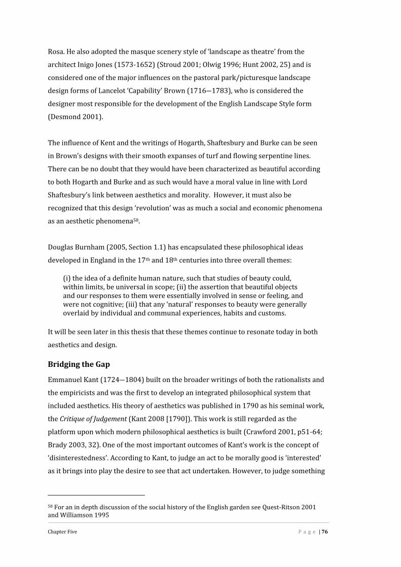
Chapter Five P a g e | 76
Rosa. He also adopted the masque scenery style of ‘landscape as theatre’ from thearchitect Inigo Jones (1573-1652) (Stroud 2001; Olwig 1996; Hunt 2002, 25) and isconsidered one of the major influences on the pastoral park/picturesque landscapedesign forms of Lancelot ‘Capability’ Brown (1716―1783), who is considered thedesigner most responsible for the development of the English Landscape Style form(Desmond 2001).The influence of Kent and the writings of Hogarth, Shaftesbury and Burke can be seenin Brown’s designs with their smooth expanses of turf and flowing serpentine lines.There can be no doubt that they would have been characterized as beautiful accordingto both Hogarth and Burke and as such would have a moral value in line with LordShaftesbury’s link between aesthetics and morality. However, it must also berecognized that this design ‘revolution’ was as much a social and economic phenomenaas an aesthetic phenomena58.Douglas Burnham (2005, Section 1.1) has encapsulated these philosophical ideasdeveloped in England in the 17th and 18th centuries into three overall themes:(i) the idea of a definite human nature, such that studies of beauty could,within limits, be universal in scope; (ii) the assertion that beautiful objectsand our responses to them were essentially involved in sense or feeling, andwere not cognitive; (iii) that any ‘natural’ responses to beauty were generallyoverlaid by individual and communal experiences, habits and customs.It will be seen later in this thesis that these themes continue to resonate today in bothaesthetics and design.Bridging the GapEmmanuel Kant (1724―1804) built on the broader writings of both the rationalists andthe empiricists and was the first to develop an integrated philosophical system thatincluded aesthetics. His theory of aesthetics was published in 1790 as his seminal work,the Critique of Judgement (Kant 2008 [1790]). This work is still regarded as theplatform upon which modern philosophical aesthetics is built (Crawford 2001, p51-64;Brady 2003, 32). One of the most important outcomes of Kant’s work is the concept of‘disinterestedness’. According to Kant, to judge an act to be morally good is ‘interested’as it brings into play the desire to see that act undertaken. However, to judge something58 For an in depth discussion of the social history of the English garden see Quest-Ritson 2001and Williamson 1995

Chapter Five P a g e | 77
as beautiful is ‘disinterested’ as it requires no personal desire to do anything about it59(Shelley 2009b, Section 1.2; Brady 2003, 34).Following Kant, the concept of beauty shifted from being seen as a sensed objectivequality to become a subjective attribute of the human mind. This shift in focus led to thedevelopment of the concept of the ‘Aesthetic Attitude’, a concept that has becameessential to the aesthetic philosophy of art. However, although Kant was interested inthe aesthetics of art, his primary interest was in the aesthetics of nature (Brady 2003,9).The perceived aesthetic value of nature diminished during the later part of the 19thcentury and the early 20th century, as the philosophy of aesthetics and the philosophyof art merged, driven by the philosophical system of Hegel that gave prominence to artover nature (Carlson 2001, 424; Inwood 2001, 67).The origins and aesthetic properties of the Beautiful and the Sublime and their impacton landscape design have been broadly touched upon above―though these are stillmatters of much philosophical and design discussion. However, it is the design forms ofthe English Pastoral Park and the Picturesque that have had the greatest long terminfluence (Howett 1987, 3; Nassauer 1992, 242; Nassauer 1997a, 68). To this end,Brady (2003, 32) argues that the 18th century was a turning point for environmentalaesthetics and states: “Changes in landscape taste reflected new philosophical ideaswhich established three aesthetic categories of nature: the beautiful, the sublime andthe picturesque.”The Picturesque and BeyondAlthough Kent is credited with the inspiration of designing landscapes as ‘pictures’, asdiscussed above, the development of the aesthetic theory of the Picturesque by theReverend William Gilpin (1724-1804) was one of the major outcomes of Burke'saesthetic dualism (Shelley 2010, Section 2.2). Discourse on the Picturesque aesthetichas tended to either focus on its relationship to artistic philosophy or its social andeconomic aspects60. However, what is missed is that as well as representing those partsof nature and landscapes that he considered ‘...capable of being illustrated by painting”59 It should be noted that Shaftesbury also felt that a judgment of beauty did not further anyform of self interest (Gill 2006)60 See Williamson 1995, Townsend 1997, Hunt 2002, Brady 2003
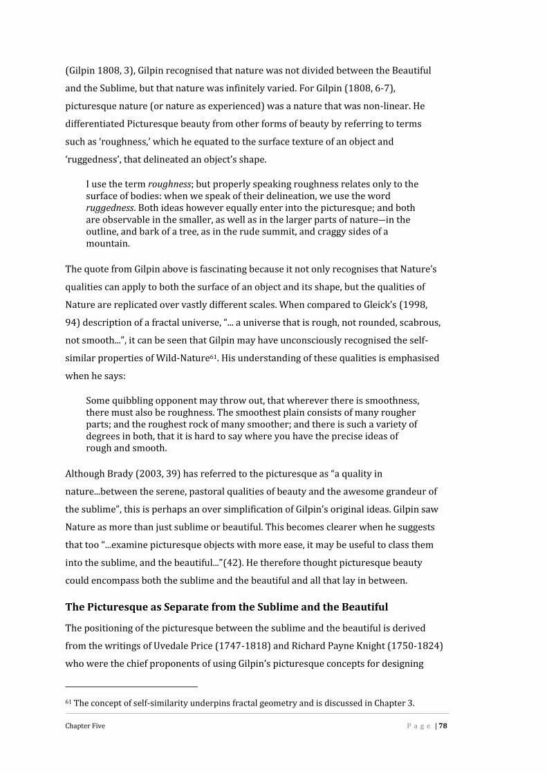
Chapter Five P a g e | 78
(Gilpin 1808, 3), Gilpin recognised that nature was not divided between the Beautifuland the Sublime, but that nature was infinitely varied. For Gilpin (1808, 6-7),picturesque nature (or nature as experienced) was a nature that was non-linear. Hedifferentiated Picturesque beauty from other forms of beauty by referring to termssuch as ‘roughness,’ which he equated to the surface texture of an object and‘ruggedness’, that delineated an object’s shape.I use the term roughness; but properly speaking roughness relates only to thesurface of bodies: when we speak of their delineation, we use the wordruggedness. Both ideas however equally enter into the picturesque; and bothare observable in the smaller, as well as in the larger parts of nature―in theoutline, and bark of a tree, as in the rude summit, and craggy sides of amountain.The quote from Gilpin above is fascinating because it not only recognises that Nature’squalities can apply to both the surface of an object and its shape, but the qualities ofNature are replicated over vastly different scales. When compared to Gleick’s (1998,94) description of a fractal universe, “... a universe that is rough, not rounded, scabrous,not smooth...”, it can be seen that Gilpin may have unconsciously recognised the self-similar properties of Wild-Nature61. His understanding of these qualities is emphasisedwhen he says:Some quibbling opponent may throw out, that wherever there is smoothness,there must also be roughness. The smoothest plain consists of many rougherparts; and the roughest rock of many smoother; and there is such a variety ofdegrees in both, that it is hard to say where you have the precise ideas ofrough and smooth.Although Brady (2003, 39) has referred to the picturesque as “a quality innature...between the serene, pastoral qualities of beauty and the awesome grandeur ofthe sublime”, this is perhaps an over simplification of Gilpin’s original ideas. Gilpin sawNature as more than just sublime or beautiful. This becomes clearer when he suggeststhat too “...examine picturesque objects with more ease, it may be useful to class theminto the sublime, and the beautiful...”(42). He therefore thought picturesque beautycould encompass both the sublime and the beautiful and all that lay in between.
The Picturesque as Separate from the Sublime and the BeautifulThe positioning of the picturesque between the sublime and the beautiful is derivedfrom the writings of Uvedale Price (1747-1818) and Richard Payne Knight (1750-1824)who were the chief proponents of using Gilpin’s picturesque concepts for designing61 The concept of self-similarity underpins fractal geometry and is discussed in Chapter 3.
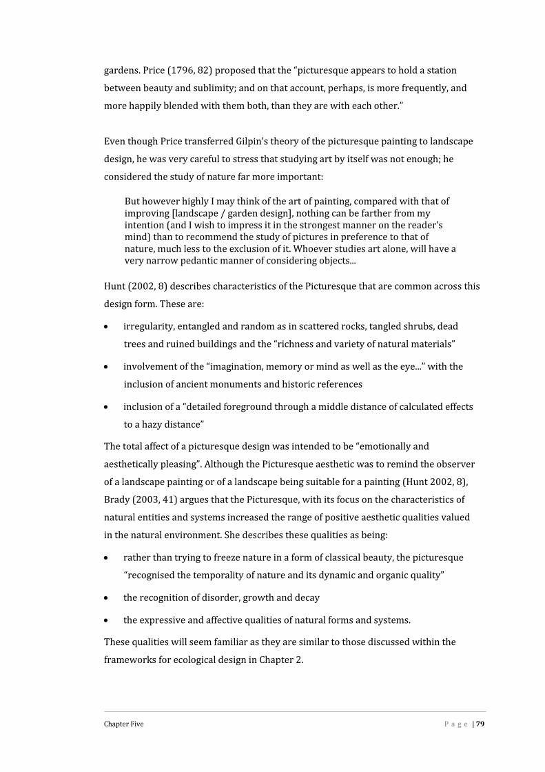
Chapter Five P a g e | 79
gardens. Price (1796, 82) proposed that the “picturesque appears to hold a stationbetween beauty and sublimity; and on that account, perhaps, is more frequently, andmore happily blended with them both, than they are with each other.”Even though Price transferred Gilpin’s theory of the picturesque painting to landscapedesign, he was very careful to stress that studying art by itself was not enough; heconsidered the study of nature far more important:But however highly I may think of the art of painting, compared with that ofimproving [landscape / garden design], nothing can be farther from myintention (and I wish to impress it in the strongest manner on the reader’smind) than to recommend the study of pictures in preference to that ofnature, much less to the exclusion of it. Whoever studies art alone, will have avery narrow pedantic manner of considering objects...Hunt (2002, 8) describes characteristics of the Picturesque that are common across thisdesign form. These are: irregularity, entangled and random as in scattered rocks, tangled shrubs, deadtrees and ruined buildings and the “richness and variety of natural materials” involvement of the “imagination, memory or mind as well as the eye...” with theinclusion of ancient monuments and historic references inclusion of a “detailed foreground through a middle distance of calculated effectsto a hazy distance”The total affect of a picturesque design was intended to be “emotionally andaesthetically pleasing”. Although the Picturesque aesthetic was to remind the observerof a landscape painting or of a landscape being suitable for a painting (Hunt 2002, 8),Brady (2003, 41) argues that the Picturesque, with its focus on the characteristics ofnatural entities and systems increased the range of positive aesthetic qualities valuedin the natural environment. She describes these qualities as being: rather than trying to freeze nature in a form of classical beauty, the picturesque“recognised the temporality of nature and its dynamic and organic quality” the recognition of disorder, growth and decay the expressive and affective qualities of natural forms and systems.These qualities will seem familiar as they are similar to those discussed within theframeworks for ecological design in Chapter 2.

Chapter Five P a g e | 80
The discussion above makes it clear that the transformational power of aesthetics tochange people’s attitudes to accepting, appreciating and even desiring differentlandscape design forms cannot be underestimated. This is essential if the forms andpatters of Wild Nature are to be re-interpreted within the context of Designed Nature.The growth and longevity of the design form commonly referred to as the English, orIdyllic Pastoral Park, culminating in the Picturesque, indicates that this is not onlypossible but achievable. These design forms were driven by an intellectual minority,but it changed the aesthetic awareness of many more to appreciate the visualproperties of Wild Nature―even if this was a romantic conception of Wild Nature.Although the idyllic pastoral park and the Picturesque were the dominant design formsof the period, during the mid to late 19th century, the science of botany and thetechniques of scientific horticulture rapidly progressed. This progress in botany,coupled with the expansion of the British Empire and the developing philosophy of art,became the new driving forces in landscape design. One of the chief exponents of thenew scientific horticulture was JC Loudon. In his book, Observations on the Formation
and Management of Useful and Ornamental Plantations on the Theory and Practice of
Landscape Gardening, published in 1804, JC Loudon (1804, 214-215) proclaimed “Ibelieve that I am the first who has set out as a landscape gardener, professing to followMr Price’s principles”.JC Loudon and the Consequences of the GardenesqueAs promised, Loudon’s early designs implemented Price’s Picturesque ideas by creatingland, water and planting designs that were ‘irregular’. However, his career as apracticing landscape designer was cut short early due to Rheumatic Fever. It is throughhis second career as an author that Loudon’s made his greatest contribution tolandscape design and elevated him to such an influential position within this field.Between 1803 and 1845 his prodigious literary output was approximately 60 millionwords (Turner 2001b).In 1822, after several tours of Europe visiting and sketching the great gardens (Turner2001b), Loudon published the first edition of Encyclopaedia of Gardening. In hisdiscussions on the history of gardening it is clear that he had moved away from thePicturesque:The modern style of gardening and the arts of poetry and painting imitatenature and in doing so the art employed is studiously concealed Those arts

Chapter Five P a g e | 81
therefore can never be compared whose means are so different and to saythat landscape gardening is an improvement on geometric gardening is asimilar misapplication of language as to say that a lawn is an improvement ona cornfield because it is substituted in its place. It is absurd therefore todespise the ancient style because it has not the same beauties at the modernto which it never aspired It has beauties of a different kind equally perfect intheir manner as those of the modern style and equally desirable under certaincircumstance The question therefore, is not, whether we shall admitoccasional specimens of obsolete gardening for the sake of antiquity, butwhether we shall admit specimens of a different style from that in general usebut equally perfect in its kind.This becomes even clearer when in the section dealing with the philosophy oflandscape design; he recognised that paintings and landscape may exhibit a differentaesthetic62:The principles of composition to be studied by the landscape gardener63 aretherefore not exactly the same as those which govern the artist and there aremany objects which produce a fine effect in park scenery which do not lookwell in a picture. For example few scenes have a more beautiful effect inpleasure grounds than a velvet lawn presenting a surface of uniformsmoothness and verdure perhaps occasionally diversified by a few swellingknolls yet how badly such a scene would look in a picture in fact it would bealmost impossible to paint it. On the other hand the rough banks of a rivercovered with tussocks of rushes large stones and stumps the groundsometimes smooth sometimes broken and abrupt and seldom keeping for along space the same level from the water though they may produce a fineeffect in a picture would be extremely unsuitable to the pleasure grounds of agentleman's residence.Loudon’s interests and expertise in botany, horticulture and agriculture, as well as hisavid collection of new and exotic plants from overseas, led him to create a new plantingdesign form that he termed the ‘gardenesque’. This was a planting design form whereeach individual plant was allowed to develop its inherent character and grow to its fullpotential without interference from other plants or structures. He first proposed thisform of planting in the December edition of the Gardener’s Magazine in 1823.Landscape Design as ArtMelanie Simo (1988) proposes that the rationale for Loudon’s development of thegardenesque, was not driven by any “grand personal ambition” to be considered as anoriginal designer or to undermine traditional forms of landscape gardening. Her62 This disparity between the aesthetics of art and the aesthetics of design landscapes are centralto Nassauer’s (1992, 247) argument that an ecological aesthetics must be based on theprogressive change of culture with respect to the experience that an ecologically sustainablelandscape should give.63 During the time of JC Loudon, the term landscape gardener was equivalent to our modern dayterm landscape designer.

Chapter Five P a g e | 82
hypothesis is that he developed the gardenesque because of his great interest in treesand shrubs as things of great beauty64. However, this rationale does not take intoaccount Loudon’s (1838, 137) desire for landscape design to be considered an art in itsown right, which is evident when he said :The great object of all human exertion, after satisfying those wants which areessential to our existence, is to procure the approbation or applause ofourselves or others. To imitate nature in such a way as that the objectproduced should be mistaken for nature, could never excite muchapprobation for the artist, because its very perfection by deceiving thespectator into a belief of its reality, would prevent it from being considered asa work of art. On the contrary, when an object is imitated in a totally differentmaterial from that in which it appears in nature, and the imitation issuccessful, the applause of the spectator is great in proportion to the degreeof skill displayed.Similarly, the concept of plants being allowed to grow into their perfect shape reflectsthe Neo-Platonic concept of ideal forms, which formed a major component of an essayon fine arts by the French philosopher Chrysostome Quatremère de Quincy (Quincy1837) published in 1823. In this essay, de Quincy built an effective aesthetic blockadeto the English Landscape Style design form being considered an art when he claimedthat landscape gardening, and particularly the English ‘irregular style’, could not beconsidered as an art because it was indistinguishable from Nature (Quincy 1837, 170):If among the number of the fine arts it be allowable to cite one which it hasnot as yet been agreed upon to call an art of imitation, I allude to landscapegardening, more especially in the irregular style, it is with a view to show thatin accordance with the spirit of this theory, it is of itself excluded from theimitative scale. In fact, every element necessary to constitute imitation isabsent from it. Even the idea of repetition is scarcely traceable. Whatpretends to be an image of nature is nothing more nor less than natureherself. The means of the art are reality.De Quincy’s position on landscape design derived from his concept of art as imitation.In essence, for something to be considered a work of art it had to be undertaken inmaterials that could not be mistaken for the actual object being depicted: “To imitate inthe fine arts, is to produce the resemblance of a thing, but in some other thing whichbecomes the image of it” (1837, 11). Therefore, the farther removed the ‘material’ ofthe art was from the object being imitated, the higher the form of art. Thus de Quincyrated poetry as the highest of all the arts followed closely by music. Then followedpainting, sculpture and architecture and finally dancing and pantomime (1837, 166-170).64 This could almost be considered an obsession, given his prodigious literary output.

Chapter Five P a g e | 83
To overcome this blockade, Loudon developed the idea that a landscape garden couldbe considered art if all indigenous vegetation, gravel, rocks and grass were replaced byplant species and materials that were sourced from outside the area. This was thegenesis of a design form that was supported by the rapid growth in horticulture, botanyand biological sciences. This radical shift in design from predominantly using localindigenous plant species and materials to predominantly using exotic plants andmaterials, was promoted in his seminal work, The Suburban Gardener and Villa
Companion (Loudon 1838) and is illustrated by the following quotes:Simply let foreign trees and shrubs, or such as are totally different from thetrees in the given locality, be planted, instead of indigenous trees; let the samebe done as to the water plants, the same as to the stones and gravel; the sameas to the slopes of the turf; the same as to the outline of the water; and, as faras practicable, the same even as to the grasses composing the lawn. (138-139)Wood, if the common trees of the locality are employed, must be eitherplanted in lines, or geometrical figures; or, if foreign trees and shrubs only areused, they may be planted in irregular masses or groups, and as single trees. Ifindigenous trees and shrubs are at any time introduced in the modern style,of landscape-gardening, the greatest care must be taken not to crowd, or evengroup, them together in such a manner as that a stranger might conclude theyhad grown up there naturally. They must be placed so as to stand distinctfrom other trees and shrub, so as to take forms more perfectly developed thanwhat the same species are found to have in a natural or accidental state in thesurrounding country. (140)Loudon’s vision of the gardenesque planting design form was never reallyimplemented, except perhaps in botanic gardens and arboretums. Instead, the termwas adopted and modified by Edward Kemp (1817-1891). In his book, How to Lay Out a
Small Garden, published in 1850 Kemp (82) described three styles of garden design;“...the old formal or geometrical style; a mixed, middle, or irregular style, which Mr,Loudon called gardenesque; and the picturesque.” Kemp’s placement of thegardenesque midway between the geometric design form (that could be considered asart) and the picturesque design forms that were more representative of nature,mirrored the positioning of the Picturesque between the beautiful and the sublime byPrice, as discussed above. It was this version of the gardenesque, composed of rampanteclecticism and lack of artistic unity (Turner 2001a), that was favoured by theVictorians and is still reiterated in design today.From an ecological position, it is clear that it is not just the Picturesque that has had amajor impact on the ecology of Western Para-natural environments, but Loudon’s

Chapter Five P a g e | 84
desire for landscape design to be recognised as an art form played a very significantrole. If Gilpin’s original definition of Picturesque beauty, as described above, iscombined with our current knowledge of ecology and environmental systems, designedlandscapes would be far more ecologically sustainable that they are at present.Aesthetics and NatureWhether Kant’s theory of the disinterestedness led to the development of thePicturesque (Carlson 2002, 4), or the Picturesque led to the development of Kant’stheory (Townsend 1997), or whether the requirement for a psychological separation ofpeople from their environment is just a facet of modern human existence is a matter fordiscussion outside this research. However, the Picturesque, which recognised theinfinite variety and dynamic temporal qualities of Wild Nature and encouraged a movetowards appreciating “nature in the raw” (Brady 2003, 41), has been criticised aspotentially un-ecological (Nassauer 1997b, 68; Howett 1987, 4) and a bankrupt ideal(Thayer 1976, 40). It has been held responsible for the objectification and a distancingof people from Wild Nature (Thompson 2009, 57). However, Cosgrove (1998) makes itclear, in his book, Social Formation and Symbolic Landscape, that the reasons for thisobjectification are much broader. Today the digital camera, video recorder, mobilephone, cinema and the ‘framed’ television can be seen to have replaced the ‘Claudeglass’ of the Romantics, so that all Nature has become deconstructed and objectifiedinto a mass consumption voyeuristic view.The perceived aesthetic value of nature diminished during the later part of the 19thcentury and the early 20th century, as the philosophy of aesthetics and the philosophyof art merged (Carlson 2001, 424). This position was maintained until the publicationof Hepburn’s (1966) seminal paper entitled Contemporary Aesthetics and the Neglect of
Natural Beauty. He states, “Open any eighteenth-century work on aesthetics, and theodds are that it will contain a substantial treatment of the beautiful, the sublime, andthe picturesque in nature65”. This renewed recognition of the aesthetic value of natureled to a more inclusive understanding of aesthetics, as articulated by that of SusanFeagin (1999, 11-12), wherein she describes aesthetics as the “branch of philosophythat examines the nature of art and the character of our experience of art and of thenatural environment”. Feagin describes the four major components of aesthetics asbeing the:65 Although Hepburn’s concept of nature refers to all objects that are not human artifacts, Idoubt if he considered the human modified pastoral or country landscape as a human artifact.

Chapter Five P a g e | 85
aesthetics experience― a special type of experience that can be differentiated fromother types of experiences aesthetic attitude― a special kind of attitude required to aesthetically appreciateart or nature. This concept is directly derived from Kant’s disinterestedness. aesthetic value― a distinctive value different from other types of values such aseconomic, religious and moral. aesthetic object―a special object that can be called aesthetic. This is related moreto art than nature.To these four components, Brady (2003, 16) and Eaton (Eaton 1992) have added whatthey call an aesthetic quality (Brady) or an aesthetic property (Eaton).The study of the aesthetic experience of nature, is now encapsulated in what is calledEnvironmental Aesthetics, which, as Carlson notes, includes the aesthetic appreciationof natural environments and “human-influenced and human-constructedenvironments” (Carlson 2001, 423). Carlson recognised environmental aesthetics asone of the “major new fields of aesthetics to emerge in the second half of the twentiethcentury”.Environmental AestheticsThe field of environmental aesthetics has significant differences from the aestheticsapplied to art objects. One of the common characteristics of all art objects are that theyare set apart from their contextual environment―they are physically and conceptually‘framed’ and separated from the perceiver. This concept of framing applies to a paintedpicture as well as to a sculpture set on a pedestal, an orchestra on a stage or a boundbook (Hepburn 1966, 290-291). Framing facilitates the recognition that what is beingperceived is, in fact, an art object. However, when we experience Nature we are, asHepburn says “...in nature and a part of nature; we do not stand over against it as overagainst a painting on a wall”. Berleant (1992) expands on this position and applies it toenvironmental aesthetics with his concept of ‘aesthetic of engagement’.Contemporary theories of environmental aesthetics can be divided into two maingroups. The first is the cognitive group which maintain that an objective, scientific
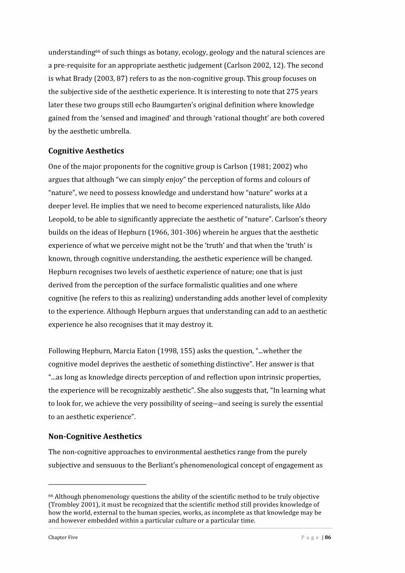
Chapter Five P a g e | 86
understanding66 of such things as botany, ecology, geology and the natural sciences area pre-requisite for an appropriate aesthetic judgement (Carlson 2002, 12). The secondis what Brady (2003, 87) refers to as the non-cognitive group. This group focuses onthe subjective side of the aesthetic experience. It is interesting to note that 275 yearslater these two groups still echo Baumgarten’s original definition where knowledgegained from the ‘sensed and imagined’ and through ‘rational thought’ are both coveredby the aesthetic umbrella.Cognitive AestheticsOne of the major proponents for the cognitive group is Carlson (1981; 2002) whoargues that although “we can simply enjoy” the perception of forms and colours of“nature”, we need to possess knowledge and understand how “nature” works at adeeper level. He implies that we need to become experienced naturalists, like AldoLeopold, to be able to significantly appreciate the aesthetic of “nature”. Carlson’s theorybuilds on the ideas of Hepburn (1966, 301-306) wherein he argues that the aestheticexperience of what we perceive might not be the ‘truth’ and that when the ‘truth‘ isknown, through cognitive understanding, the aesthetic experience will be changed.Hepburn recognises two levels of aesthetic experience of nature; one that is justderived from the perception of the surface formalistic qualities and one wherecognitive (he refers to this as realizing) understanding adds another level of complexityto the experience. Although Hepburn argues that understanding can add to an aestheticexperience he also recognises that it may destroy it.Following Hepburn, Marcia Eaton (1998, 155) asks the question, “...whether thecognitive model deprives the aesthetic of something distinctive”. Her answer is that“...as long as knowledge directs perception of and reflection upon intrinsic properties,the experience will be recognizably aesthetic”. She also suggests that, “In learning whatto look for, we achieve the very possibility of seeing―and seeing is surely the essentialto an aesthetic experience”.Non-Cognitive AestheticsThe non-cognitive approaches to environmental aesthetics range from the purelysubjective and sensuous to the Berliant’s phenomenological concept of engagement as66 Although phenomenology questions the ability of the scientific method to be truly objective(Trombley 2001), it must be recognized that the scientific method still provides knowledge ofhow the world, external to the human species, works, as incomplete as that knowledge may beand however embedded within a particular culture or a particular time.
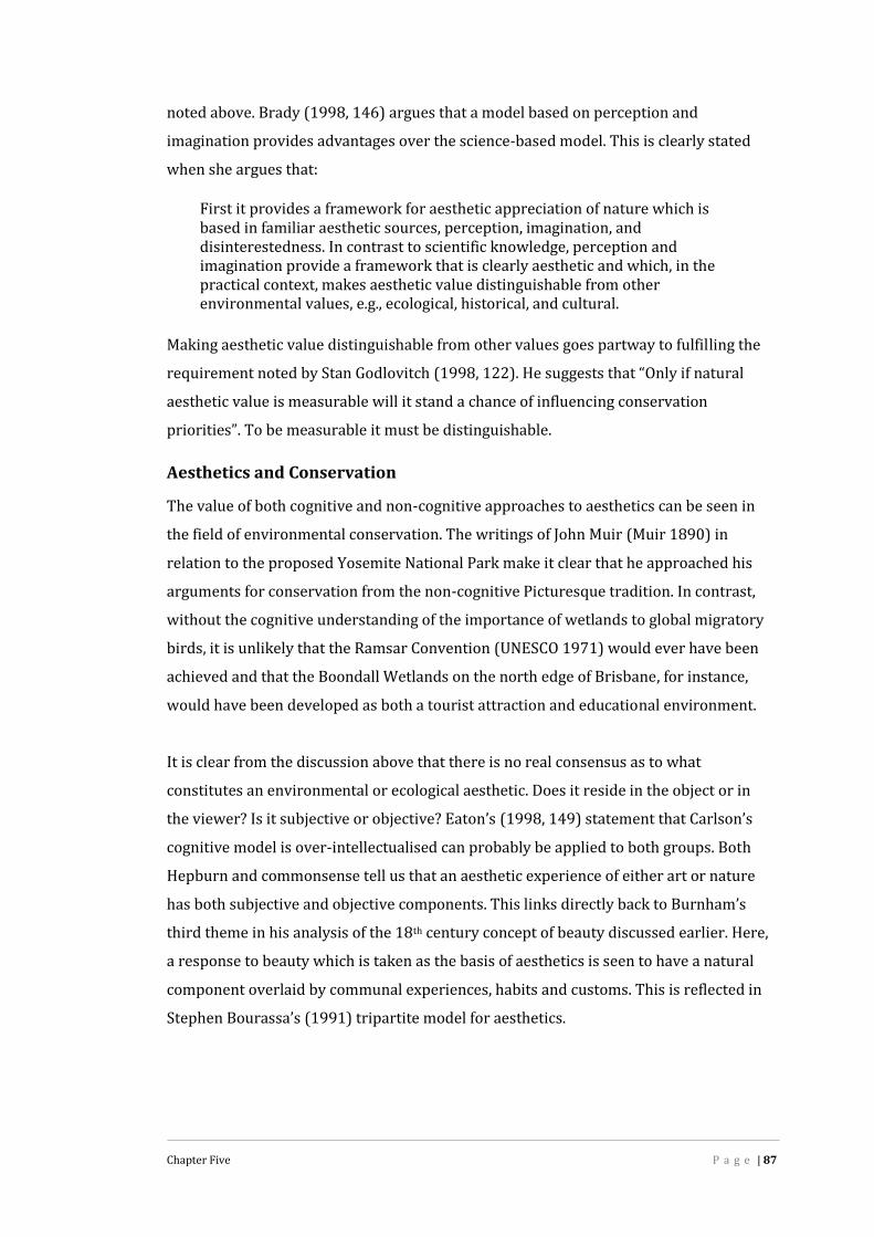
Chapter Five P a g e | 87
noted above. Brady (1998, 146) argues that a model based on perception andimagination provides advantages over the science-based model. This is clearly statedwhen she argues that:First it provides a framework for aesthetic appreciation of nature which isbased in familiar aesthetic sources, perception, imagination, anddisinterestedness. In contrast to scientific knowledge, perception andimagination provide a framework that is clearly aesthetic and which, in thepractical context, makes aesthetic value distinguishable from otherenvironmental values, e.g., ecological, historical, and cultural.Making aesthetic value distinguishable from other values goes partway to fulfilling therequirement noted by Stan Godlovitch (1998, 122). He suggests that “Only if naturalaesthetic value is measurable will it stand a chance of influencing conservationpriorities”. To be measurable it must be distinguishable.Aesthetics and ConservationThe value of both cognitive and non-cognitive approaches to aesthetics can be seen inthe field of environmental conservation. The writings of John Muir (Muir 1890) inrelation to the proposed Yosemite National Park make it clear that he approached hisarguments for conservation from the non-cognitive Picturesque tradition. In contrast,without the cognitive understanding of the importance of wetlands to global migratorybirds, it is unlikely that the Ramsar Convention (UNESCO 1971) would ever have beenachieved and that the Boondall Wetlands on the north edge of Brisbane, for instance,would have been developed as both a tourist attraction and educational environment.It is clear from the discussion above that there is no real consensus as to whatconstitutes an environmental or ecological aesthetic. Does it reside in the object or inthe viewer? Is it subjective or objective? Eaton’s (1998, 149) statement that Carlson’scognitive model is over-intellectualised can probably be applied to both groups. BothHepburn and commonsense tell us that an aesthetic experience of either art or naturehas both subjective and objective components. This links directly back to Burnham’sthird theme in his analysis of the 18th century concept of beauty discussed earlier. Here,a response to beauty which is taken as the basis of aesthetics is seen to have a naturalcomponent overlaid by communal experiences, habits and customs. This is reflected inStephen Bourassa’s (1991) tripartite model for aesthetics.
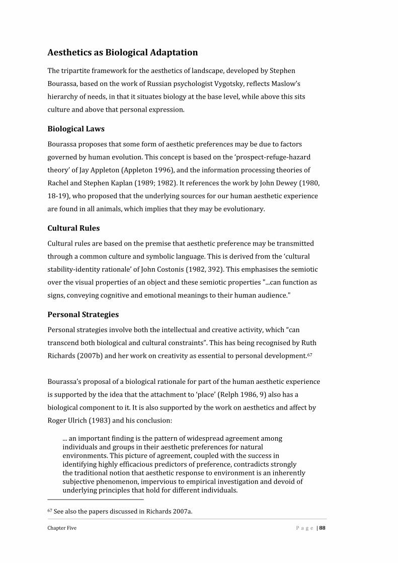
Chapter Five P a g e | 88
Aesthetics as Biological AdaptationThe tripartite framework for the aesthetics of landscape, developed by StephenBourassa, based on the work of Russian psychologist Vygotsky, reflects Maslow’shierarchy of needs, in that it situates biology at the base level, while above this sitsculture and above that personal expression.Biological LawsBourassa proposes that some form of aesthetic preferences may be due to factorsgoverned by human evolution. This concept is based on the ‘prospect-refuge-hazardtheory’ of Jay Appleton (Appleton 1996), and the information processing theories ofRachel and Stephen Kaplan (1989; 1982). It references the work by John Dewey (1980,18-19), who proposed that the underlying sources for our human aesthetic experienceare found in all animals, which implies that they may be evolutionary.Cultural RulesCultural rules are based on the premise that aesthetic preference may be transmittedthrough a common culture and symbolic language. This is derived from the ‘culturalstability-identity rationale’ of John Costonis (1982, 392). This emphasises the semioticover the visual properties of an object and these semiotic properties "...can function assigns, conveying cognitive and emotional meanings to their human audience."Personal StrategiesPersonal strategies involve both the intellectual and creative activity, which “cantranscend both biological and cultural constraints”. This has being recognised by RuthRichards (2007b) and her work on creativity as essential to personal development.67Bourassa’s proposal of a biological rationale for part of the human aesthetic experienceis supported by the idea that the attachment to ‘place’ (Relph 1986, 9) also has abiological component to it. It is also supported by the work on aesthetics and affect byRoger Ulrich (1983) and his conclusion:... an important finding is the pattern of widespread agreement amongindividuals and groups in their aesthetic preferences for naturalenvironments. This picture of agreement, coupled with the success inidentifying highly efficacious predictors of preference, contradicts stronglythe traditional notion that aesthetic response to environment is an inherentlysubjective phenomenon, impervious to empirical investigation and devoid ofunderlying principles that hold for different individuals.67 See also the papers discussed in Richards 2007a.

Chapter Five P a g e | 89
Ulrich’s position is supported by the landscape preference work undertaken by DawnHill and Terry Daniels (2008) who found that ecological information had no effect onaltering landscape aesthetic preference. They concluded that:The data are more consistent instead with the notion that aestheticpreferences for natural (or naturalistic) landscapes are mediated by affectiveprocesses, perhaps developed by natural selection during human evolution,that are relatively independent of the influences of contemporary informationinterventions or rational arguments.And as discussed in Chapter 3, it is fractal geometry that can describe the patterns ofWild Nature.Beauty, Aesthetics and Fractal PatterningThe beauty of complex fractal forms has been recognised by many, and is responsiblefor a new type of abstract art based on computer generated fractal images (Briggs, J1992). In a wider perspective, Ruth Richards (2001) takes the position that aestheticsand beauty can assist the human species to “adapt, evolve, and cope withenvironmental crises” through the recognition that humans participate in beauty as“open systems in ongoing process, coevolving with all of existence”.This position echoes the concepts of Cultural Ecology discussed in Chapter 3. Richards’paper argues that an aesthetic appreciation of beauty is not a static process, but adynamic one that in some way changes us as individuals. Through her study ofaesthetic preference, Richards links Kant’s concept of the sublime with chaos theoryand fractal geometry, and argues for a new humanistic aesthetic for environmentalawareness based on this geometry.Similarly, Joan Iverson Nassauer (1997a, 74), when arguing her case for an aestheticthat takes into account the concept of care in urban environments, supports Richardswhen she says:To most people aesthetics implies trivial decoration, and social conformityseems to contradict social change. But philosophers convincingly argue thataesthetics has a fundamental effect on how we see the world, and naturalistsand ecologists who are interested in protecting the landscape have reachedthe same conclusion.Recent studies into fractal geometry and human perception suggests that not only dohumans prefer fractal images, but that we have a physiological response to them aswell (Spehar et al. 2003; Taylor et al. 2005). The study by Taylor et al also proposes

Chapter Five P a g e | 90
that there are three ranges of aesthetic preference for fractal images, not affected bygender or cultural background, based on a one-dimensional fractal analysis. These are Low preference: fractal dimension 1.1 > 1.2 High preference: fractal dimension 1.3 > 1.5 Low preference: fractal dimension 1.6 > 1.9There is also some evidence to suggest that highly artistic people have a preference forimages with a higher fractal index than others (Richards 2001; Taylor 2002).Work has also been undertaken on how the human visual system responds to fractalpatterning. Several authors support the theory that human visual perception is tuned tothe statistical self-similarity of natural forms (Spehar et al. 2003; Billock 2000; Knill et
al. 1990). If this is the case, it would help explain the results obtained by otherresearchers when they argue that the restorative value of a landscape may beassociated with its fractal properties Purcell et al (2001), or wherein they conclude thatour preference for natural forms is the result of human evolution (Ulrich 1983; Hill andDaniel 2008; Hartmann and Apaolaza-Ibanez 2009).A Problematic AestheticGiven the discussion on aesthetics, it can be seen that there are some direct linkagesbetween ecology and aesthetics. Aesthetics can be thought of as one area of therelationship between the human species and their environment at both the biologicaland cultural levels. From this discussion it seems apparent that an aesthetic experienceor response will depend on both cognitive and non-cognitive elements. This is implicitin Thayer’s (2002, 189) argument that the transition to a sustainable world can only bebased on the “perception and comprehension of the ordinary people”. However, it isunrealistic to expect that all ‘ordinary people’ will become expert naturalists.The non-cognitive based approach that sees an aesthetic response as being perceptualrather than intellectual and which results in a response that gives pleasure whenperceiving beauty, and a response that is unpleasant when perceiving ugliness (Brady2003, 6-16), overcomes the idea that we all need to become experts to appreciateNatural environments. Treib (1995, 58) implicitly supports this view when herecognises that pleasure as a human response is ignored by most design discourse.

Chapter Five P a g e | 91
Whether an aesthetic is based on a cognitive or non-cognitive basis, it is clear that it is ahuman response to something. Eaton (1992, 3) defines an aesthetic property asA is an aesthetic property of a work , W, in a culture, C, if and only if A is anintrinsic property of W and A is considered worthy of attention in C, that is, inC it is generally believed that attending to A (perceiving and/or reflecting)upon A will reward attention.This statement is clear when discussing the aesthetics of art, because as discussedabove, a work of art is ‘framed’ and completely distinguishable from its surroundings.However, when discussing the aesthetics of Nature or the aesthetics of an environmentthere has not been, as discussed Chapter 2, a clear distinction as to what Nature orwhat type of environment is being referred to. Similarly, Eaton’s definition of anaesthetic property implies that the perceiver must be consciously aware of theproperty to give it attention. However, as Rudolf Arnheim (1974, 98) has argued, therecognition of a visual object is dependent on an unconsciously perceived “structuralskeleton” that is created by the overall shape of something. Therefore, an aestheticproperty may not require conscious recognition to create an aesthetic response orexperience within an observer.What is clear is that an aesthetic experience or response is a multifaceted quality.Figure 5.1 shows the authors conceptual understanding of the potential perceptual andpsychological factors that combine in an infinite number of ways to create an aestheticexperience or response within a person at any particular time.
Figure 5. 1: Factors Involved in an Aesthetic ExperienceSensory perception clearly provides the basis for our experience of our environment.This physical experience is interpreted and modulated by our cognition, emotion,memory and imagination to create our aesthetic response.
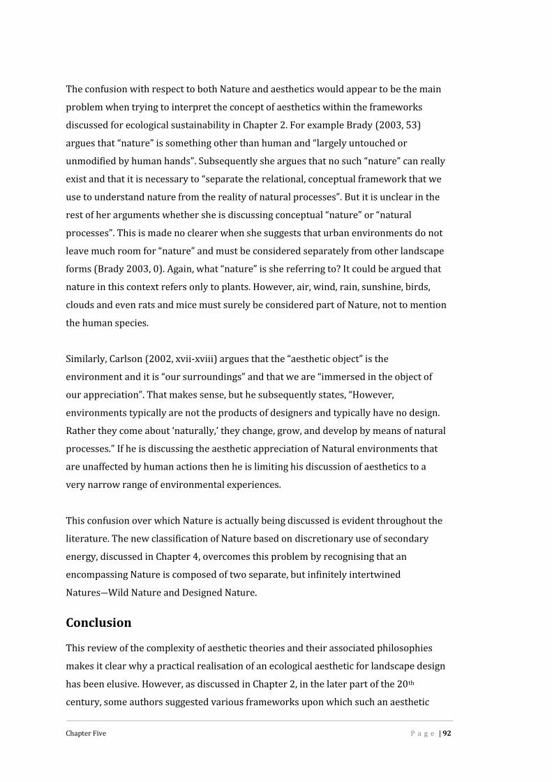
Chapter Five P a g e | 92
The confusion with respect to both Nature and aesthetics would appear to be the mainproblem when trying to interpret the concept of aesthetics within the frameworksdiscussed for ecological sustainability in Chapter 2. For example Brady (2003, 53)argues that “nature” is something other than human and “largely untouched orunmodified by human hands”. Subsequently she argues that no such “nature” can reallyexist and that it is necessary to “separate the relational, conceptual framework that weuse to understand nature from the reality of natural processes”. But it is unclear in therest of her arguments whether she is discussing conceptual “nature” or “naturalprocesses”. This is made no clearer when she suggests that urban environments do notleave much room for “nature” and must be considered separately from other landscapeforms (Brady 2003, 0). Again, what “nature” is she referring to? It could be argued thatnature in this context refers only to plants. However, air, wind, rain, sunshine, birds,clouds and even rats and mice must surely be considered part of Nature, not to mentionthe human species.Similarly, Carlson (2002, xvii-xviii) argues that the “aesthetic object” is theenvironment and it is “our surroundings” and that we are “immersed in the object ofour appreciation”. That makes sense, but he subsequently states, “However,environments typically are not the products of designers and typically have no design.Rather they come about ‘naturally,’ they change, grow, and develop by means of naturalprocesses.” If he is discussing the aesthetic appreciation of Natural environments thatare unaffected by human actions then he is limiting his discussion of aesthetics to avery narrow range of environmental experiences.This confusion over which Nature is actually being discussed is evident throughout theliterature. The new classification of Nature based on discretionary use of secondaryenergy, discussed in Chapter 4, overcomes this problem by recognising that anencompassing Nature is composed of two separate, but infinitely intertwinedNatures―Wild Nature and Designed Nature.ConclusionThis review of the complexity of aesthetic theories and their associated philosophiesmakes it clear why a practical realisation of an ecological aesthetic for landscape designhas been elusive. However, as discussed in Chapter 2, in the later part of the 20thcentury, some authors suggested various frameworks upon which such an aesthetic

Chapter Five P a g e | 93
might be based. It has been argued that within many of these frameworks there is anunderlying theme: that the space-time patterns of natural systems and processes mayform the basis for an aesthetic for sustainable landscape design. Although Koh (1988,180) examined this problem and proposed that “An ecological theory of environmentaldesign must be based on ordering principles in nature and on human perception andcognition”, Thayer (1989, 104) makes it clear that the then current visual and spatialdesign languages were not capable of articulating the complexity of sustainablesystems.Christopher Alexander (2002, 1) expanded on this concept when he stated that “Ourworld is dominated by the order we create”. He argued that even though we createorder through the act of building, we do not really understand what order is and thatwe need a much better understanding of the “deep geometric reality of order” to enableus to design and build human systems that create sustainable life. As part of his searchfor a unified theory of order, Alexander identified 15 fundamental properties, many ofwhich are strongly related to the forms and patterns found in natural systems andprocesses that are described by fractal geometry.As discussed previously, Thayer (1989, 104) questioned the ability of fractal geometryto act as “the visual and spatial vocabulary to express and interpret the evolvingcomplexity and "invisibility" of nature in landscape design...”. However, what Thayerand Alexander seem to miss is that the fractal patterns produced by Wild Nature arethe physical embodiment and a form of order, which results from the systems andprocesses of Wild Nature. Therefore, although fractal geometry has not, as yet, beenconsciously used to create landscape design solutions, a greater understanding of thedifference between the patterns and forms produced by Wild Nature and those byDesigned Nature is essential to understand the basic differences between their deepgeometric order and how fractal geometry can be used as a referent for landscapedesign.The discussion in Chapter 4 recognised that landscapes are structurally very complex,consisting of both Natural and Para-natural environments, which when viewed at streetlevel are arrayed in multiple visual planes. An added complication is that landscapesare very rarely viewed from a single position or at a single point in time, but are viewedfrom multiple positions over periods of time. Therefore, in order to compare thegeometry of different landscape forms, a measure of the overall, or composite, fractal

Chapter Five P a g e | 94
dimension of a landscape is required. However, in order to achieve this, it is firstnecessary to understand how the fractal dimension of a complex spatial entity can bedetermined. This is discussed in the following chapter

Chapter Six P a g e | 95
Chapter Six
Measuring the Fractal Dimension of a Landscape
The tree which moves some to tears of joy is in the eyes of others only agreen thing that stands in the way. Some see nature all ridicule and
deformity... and some scarce see nature at all. But to the eyes of the manof imagination, nature is imagination itself. (William Blake 1757-1827)68
IntroductionThe fractal dimension of an entity can be determined in many ways, depending on theentity in question. The methods range from a simple Divider-Compass method formeasuring the fractal dimension of a coastline, as discussed in Chapter 3, to highlycomplex mathematical and statistical methods for determining the fractal dimension ofboth temporal and spatial signals69. One of the most common methods, the BoxCounting Method, has been used to analyse architectural forms (Bovill 1996; Lorenz2009), the textural complexity of urban street scenes (Cooper et al. 2010; Cooper andOskrochi 2008)and ecological habitats (Kenkel and Walker 1996).An example of this method is given below, which serves to highlight the potentialdifference in the fractal like patterning of the Gardenesque and Picturesque plantinglayouts described by John Loudon (1838, 164-165) in his book The Suburban Gardener,
and Villa Companion.The Box Counting MethodFigure 6.1 shows Loudon’s plan graphic interpretation of his Gardenesque plantingform and a Picturesque planting form, within the same spatial location. It is interestingto note that in the gardenesque mode, he describes the path edges as “definite andsmooth”, while in the Picturesque mode, he describes them as “indefinite and rough”.Given the discussion on Loudon’s Gardenesque design form in Chapter 5, it can be seenthat many landscape design forms today are a blend of the Gardenesque andPicturesque.68 William Blake. BrainyQuote.com, Xplore Inc, 2010.http://www.brainyquote.com/quotes/quotes/w/williambla139060.html, accessed September23, 2010.69 For a comprehensive review of the most common methods used see Kenkel and Walker 1996

Chapter Six P a g e | 96
Gardenesque Picturesque
Figure 6. 1: Loudon’s Interpretation of Gardenesque and Picturesque PlantingTo use the box counting method to determine the fractal dimension of these plans, agrid is overlaid onto the images and the number of grid squares that intersect with apart of a plant graphic is counted. This is done for grids of consecutively smaller sizes,as show in Figure 6.2.Gardenesque Picturesque
Box 1: N=45, g=10 Box 1: N=38. g=10
Box 2: N=128, g=20 Box 2: N=120, g=20
Box 3: N=345, g=40 Box 3: N=337, g=40
Box 4: N=938, g=80 Box 4: N=1042, g=80
Figure 6. 2: Box Counting Grids and Counts

Chapter Six P a g e | 97
Where, N equals the number of grid squares that are intersected by a part of a plantgraphic and g equals the number of grid squares along the horizontal axis. Given thesetwo numbers, the fractal dimension is calculated by the following equation:The results for this analysis are shown in Table 6.1.
Table 6. 1: Box Counting Results
Gardenesque Picturesque
D(Box Grid 2 – Box Grid 1) = 1.53 D(Box Grid 2 – Box Grid 1) = 1.66
D(Box Grid 3 – Box Grid 2) = 1.45 D(Box Grid 3 – Box Grid 2) = 1.49
D(Box Grid 4 – Box Grid 3) = 1.47 D(Box Grid 4 – Box Grid 3) = 1.63
Average = 1.48 Average = 1.59
It can be seen in this example, that the fractal dimension for Loudon’s graphicinterpretation of a Picturesque planting form is higher than for his gardenesque form.With smaller and smaller grids, this difference would increase, because the Picturesqueform exhibits higher complexity at the edges than the gardenesque. This is very similarto the measurement of a coastline discussed in Chapter Five.When trying to determine the fractal dimension of an entity, the common elementamongst all of the methods is the use of a surrogate, as seen in the example above. Asfar as the author is aware, the direct measurement of the fractal dimension of complex,three dimensional spatial entities is not feasible. Thus, in all applications, it is thefractal dimension of the surrogate that is measured and the fractal dimension of theactual one, two or three-dimensional entity is inferred from that―and in most cases isassumed to be equivalent.As discussed in Chapter 1, this research is based on the geometric analysis of landscapeform rather than on landscape assessment in terms of user experience or preference.Therefore, the surrogate used to determine the fractal dimension of a landscape is thedigital photographic image.

Chapter Six P a g e | 98
The Fractal Dimension of a Digital ImageAlex Pentland (1984, 664) has shown that provided a three dimensional surface ishomogeneous, “...the fractal dimension of the surface normal70 dictates the fractaldimension of the image intensity surface and, of course, the dimension of the physicalsurface”. Thus, the luminance intensity of the surface of a range of images will reflectthe same range of fractal dimensions as the actual three-dimension entitiesphotographed. One advantage of analysing the image luminance properties of anenvironment, is that it conveys information that relates to the texture (or roughness) ofthe environment and Pentland (1984, 664) has shown that there is a high correlationbetween fractal dimension and perceived roughness.With respect to the requirement for homogeneity, however, he also states (665) that“even if the surface is not homogeneous or uniformly illuminated, however, we can stillhope to infer the fractal dimension of the surface from the images contours andbounding contours”. Therefore, from this work we can infer that a digital photographicimage will be an acceptable surrogate for the fractal analysis of both Natural and Para-natural environments, even though their surface will not always be homogeneous oruniformly illuminated.Although easy to use, the Box Counting method previously discussed can only derivethe one-dimensional fractal dimension of a complex spatial entity based on the edgesembedded within a digital image and as such has recognised limitations associatedwith accuracy (Cooper and Oskrochi 2008, 353; Kenkel and Walker 1996, 82). Whenusing Box Counting to analyse images, edge detection methods must be used. Thisprocess can remove a significant amount of spatial information embedded within eachimage. Therefore, in this thesis the method used to estimate the fractal dimension of adigital photographic image is based on the field of mathematics known as Fourieranalysis.Fourier AnalysisFourier analysis was developed by Joseph Fourier (1768–1830) and is now a highlycomplex area of mathematics. It is far beyond the abilities of the author or the scope ofthis research to describe in detail. However, a basic knowledge of this analysis70 Viewed at 90 degrees to the surface plane

Chapter Six P a g e | 99
technique71 is required in order to understand the results of the research described inChapter Seven.Fourier analysis is a mathematical process that transforms complex real-world signals,such as an audio waves, into their component frequencies. If the original signal isperiodic, for example a sine wave, then the Fourier analysis and its output are calledthe Fourier Series. If the original signal is not periodic, for example a photographicimage, then Fourier analysis and its output are called the Fourier Transform. Theoutput of the Fourier transform is an image that represents the frequency componentsand their magnitude embedded within the structural geometry of the image. TheFourier transform image is the frequency domain representation of the original spatialimage.However, understanding the Fourier Series is essential to understanding the Fouriertransform.The Fourier SeriesFourier theory states that any periodic signal, such as an acoustic wave orelectromagnetic wave or any form of vibration, can be expressed as the sum of a seriesof sinusoidal signals with frequency f and amplitude A. This is equivalent to describinga musical chord played on a piano, which is composed of different notes each with theirown frequency.This mathematical transformation, called the Fourier Series, is depicted in Figure 6.3,which shows a square wave and the first four frequency components. Although for anideal square wave the frequency components will tend towards infinity; this isimpossible in reality.
71 The information used to understand Fourier analysis and image transformations comes fromthe following sources:http://en.wikipedia.org/wiki/Fourier_transform,http://en.wikipedia.org/wiki/Fourier_analysis,http://sharp.bu.edu/~slehar/fourier/fourier.html,http://homepages.inf.ed.ac.uk/rbf/HIPR2/fourier.htm,http://www.cs.unm.edu/~brayer/vision/fourier.html.

Chapter Six P a g e | 100
Figure 6. 3: Fourier Series for a Square Wave of FrequencyFigure 6.4 shows the reverse, where the component frequencies f, 3f, 5f, and 7f areadded together to reform the original square wave. It can be seen that the frequencywith the largest amplitude has the same periodicity as the original square wave and asthe frequencies get higher their amplitude drops.
f f + 3f
f+ 3f + 5f f + 3f + 5f + 7f
Figure 6. 4: Fourier AdditionAnother way to understand this process is to consider a musical chord played on thepiano. Each note in a musical chord is a separate frequency, but what you hear is acomposite sound. Each separate note contributes to that sound.From the Fourier Series, it is possible to determine the power spectrum containedwithin the original signal. The power spectrum p(f), expresses how the power of a

Chapter Six P a g e | 101
signal is distributed between the separate frequency components derived from theFourier Series, where power of any particular frequency component is defined as thesquared value of its amplitude. Figure 6.5 shows the one dimensional power spectrumfor the first four frequency components of the square wave shown in Figure 6.3.
Figure 6. 5: One Dimensional Fourier Power SpectrumAlthough this transformation seems reasonably understandable for one-dimensionalsignals such as acoustic waves and electromagnetic waves, it is harder to see how thiscan be applied to digital photographic images, which are a representation of a three-dimensional physical space in a two dimensional plane.The One-Dimensional Fourier Transform and the Fractal Dimension of
Digital ImagesTo determine the two-dimensional fractal dimension of a 24 bit colour digitalphotographic image using the Fourier Transform, the image is first converted to aneight (8) bit grey scale colour mode. This colour mode gives luminous intensity valuesfor each image pixel in the range 0 to 255, where 0 represents black and 255 representswhite. It does not include any chromatic, or colour, variation. If the values for each pixelwithin a row or column are plotted on a graph, a line with a specific frequencysignature is obtained. This process is demonstrated for the image shown in Figures 6.6.
Figure 6. 6: Original Image Converted to Grey Scale

Chapter Six P a g e | 102
The area identified in Figure 6.7 by the red dot is shown in more detail in Figure 6.7.Here we can see an enlargement of the original image that runs from Rows 984 to 1011and from columns 1786 to 1817.
Figure 6. 7: Magnified Section Showing Grey Scale PixelsTable 6.2 below lists the pixel grey scale values for each pixel along row 997 in Figure.Table 6. 2: Pixel Values for Row 997
Column Value Column Value Column Value Column Value
1786 147 1795 217 1803 145 1811 74
1787 160 1796 218 1804 205 1812 91
1788 170 1797 183 1805 249 1813 941790 170 1798 168 1806 245 1814 72
1791 174 1799 164 1807 243 1815 62
1792 164 1800 165 1808 243 1816 71
1793 168 1801 165 1809 251 1817 66
1794 185 1802 158 1810 199
These values can then be plotted as a graph that demonstrates the conversion of thegreyscale pixel values to a frequency curve. This is shown in Figure 6.8, where thevertical axis is the pixel value and the horizontal axis is the column number.It can be seen that adjacent pixels that have similar values result in a relativelysmoother signal, while adjacent pixels with very different values result in a signal withsteeper slopes and hence higher component frequencies, as demonstrated in the squarewave example in Figure 6.3.

Chapter Six P a g e | 103
Figure 6. 8: Converting Image Pixel Values to Frequency SignalThis conversion from pixel value to frequency is undertaken for each row and columnwithin a digital image, as part of a one-dimensional Fourier transform analysis, todetermine the amplitude of the individual Fourier frequency components (f) containedwithin each row and column. From this, the power spectrum p(f), which as notedbefore is proportional to the square of the amplitude for each component frequency, iscalculated.The fractal dimension of any particular row or column within an image is related to theslope of the ‘line of best’ fit when p(f) and f are plotted on a log-log graph (Turner et al.1998, 114). This is shown in Figure 6.9 for Row 997, where the red line is the line ofbest fit.
Figure 6. 9: One Dimensional Power Spectrum for Row 997
0
50
100
150
200
250
Pixel Value

Chapter Six P a g e | 104
The one-dimensional fractal dimension for each row or column can be calculated fromthe formulae: D1= ( + ) ÷where is the slope of the line72, and D1 is the one-dimensional fractal dimension Thecomposite two-dimensional fractal dimension of each image is then calculated using amathematical process called vertical slice averaging (Turner et al. 1998, 49-50) usingthe formula: D2= 1 + D1Where D1 is the average of all one-dimensional fractal dimensions for each row andcolumn within an image and D2 is the estimated two-dimensional fractal dimension ofthe image.It can be seen from the above discussion that the measured fractal dimension of adigital image is dependent on the ratio of the pixel-to-pixel luminous intensity valuesalong each row and column within that image. From this, it can be concluded that thequality of the digital images and any pre-possessing by the camera used in this researchwill have a significant effect on the results. This conclusion resulted in two decisionsbeing taken:1. Only one high quality camera would be used in this research to keep all imageprocessing within the camera software unified.2. An analysis was undertaken on the chosen camera to understand how the differentpicture ‘record modes’ would affect the image quality. The camera, analysis and theresultant camera settings are discussed in Appendix A, Section 1.Using the chosen camera with the appropriate settings, photographs of landscape weretaken at eye level with the camera pointing horizontally, as shown in Figure 6.11.To overcome the problem of analysing a landscape from a single viewpoint,photographs of each landscape were taken from random viewpoints over a period ofbetween one and several hours. The number of images taken within each landscapeused within this research ranged from 22 to 91.72 The slope of the line is a negative value
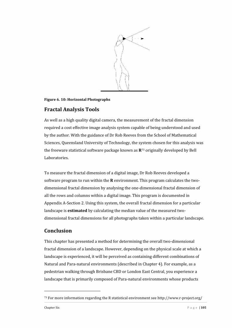
Chapter Six P a g e | 105
Figure 6. 10: Horizontal Photographs
Fractal Analysis ToolsAs well as a high quality digital camera, the measurement of the fractal dimensionrequired a cost effective image analysis system capable of being understood and usedby the author. With the guidance of Dr Rob Reeves from the School of MathematicalSciences, Queensland University of Technology, the system chosen for this analysis wasthe freeware statistical software package known as R73 originally developed by BellLaboratories.To measure the fractal dimension of a digital image, Dr Rob Reeves developed asoftware program to run within the R environment. This program calculates the two-dimensional fractal dimension by analysing the one-dimensional fractal dimension ofall the rows and columns within a digital image. This program is documented inAppendix A-Section 2. Using this system, the overall fractal dimension for a particularlandscape is estimated by calculating the median value of the measured two-dimensional fractal dimensions for all photographs taken within a particular landscape.ConclusionThis chapter has presented a method for determining the overall two-dimensionalfractal dimension of a landscape. However, depending on the physical scale at which alandscape is experienced, it will be perceived as containing different combinations ofNatural and Para-natural environments (described in Chapter 4). For example, as apedestrian walking through Brisbane CBD or London East Central, you experience alandscape that is primarily composed of Para-natural environments whose products73 For more information regarding the R statistical environment see http://www.r-project.org/

Chapter Six P a g e | 106
and processes are based principally on secondary energy sources. In contrast, hikingthrough the Lamington National Park within the Scenic Rim on the border of South EastQueensland, you would experience a landscape that is primarily composed of Naturalenvironments whose products and processes are based principally on primary energysources. From the top of any of the tall buildings within the Brisbane CBD, thepanoramic landscape experienced will contain a mix of both Natural and Para-naturalenvironments. The 360 degree view will extend from Moreton Bay to the east ofBrisbane, the Mountains of the Scenic Rim to the south and south-west, the BrisbaneRanges to the west and the Glasshouse Mountains to the north. In other words, thescale at which a landscape is experienced affects how that landscape is experienced anddescribed and whether it is considered natural or not.Because non-linear processes are the basis for many of the patterns found in WildNature, we may hypothesise that the fractal dimension is a measure of the naturalnessof a landscape (Hagerhall et al. 2004; Purcell et al. 2001). This concept is supported byLi (2000) when he suggests that the visual patterns produced by natural systems andprocesses may be important factors in identifying ecological diversity, stability andfunction. Therefore, what is required is a way to compare the overall fractal dimensionof any landscape studied with a measurable quality that differentiates between Naturalenvironments and Para-natural environments. Such a method is the focus of the nextchapter.

Chapter Seven P a g e | 107
Chapter Seven
Rating a Landscape
Nature is a continuum, with wilderness at one pole and the city at theother. The same natural processes operate in the wilderness and in the
city. (Spirn 1947)
IntroductionThe conception of ‘natural’ is a value judgement based on cultural concepts andindividual experiences embodied in the bipolar terms - natural vs. unnatural. However,it is clear from the quote by Anne Whiston Spirn at the start of this chapter, and thediscussion so far, that this conception of bipolar opposites is erroneous. Naturalprocesses operate across all landscape types and across all scales. Therefore, the ratingscale for this research embodies that ideas, discussed in Chapter 3, that landscapes area combination of both Natural and Para-natural environments. The more Naturalenvironments within a landscape, the closer it is to Wild Nature, the more Para-naturalenvironments within a landscape the closer it becomes too Designed Nature Thisreinforces the concepts that there is not a single step from Wild Nature to DesignedNature, that all environments exists within the same continuum and that DesignedNature cannot exist without the support of Wild Nature. Such a scale is shown in Figure7.1.The broad definitions derived for this scale are shown in Table 7.1. From Chapters 2and 3, it can be seen that a rating level for a landscape composed of either Wild Natureor Designed Nature in isolation cannot be justified. The two are inextricably linked dueto the global and all pervasive impact humans have on the environment.Table 7. 1: Landscape Rating
Rating Broad Definition5 Primarily Natural Environments with minor intrusions of Para-natural environments4 Mainly Natural Environments with moderate intrusions of Para-natural environments3 A clearly defined mix of Natural and Para-natural Environments2 Mainly Para-natural Environments with moderate intrusions of Natural Environments1 Primarily Para-natural environments with minor intrusions of Natural Environments
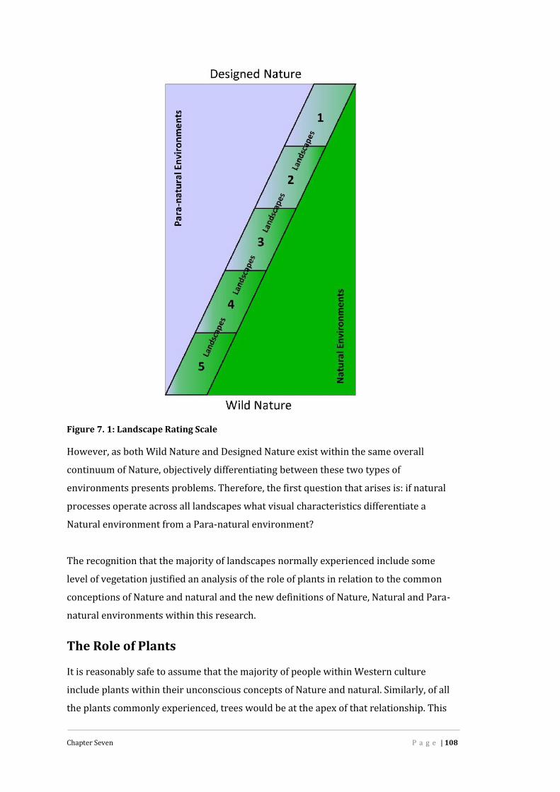
Chapter Seven P a g e | 108
Figure 7. 1: Landscape Rating ScaleHowever, as both Wild Nature and Designed Nature exist within the same overallcontinuum of Nature, objectively differentiating between these two types ofenvironments presents problems. Therefore, the first question that arises is: if naturalprocesses operate across all landscapes what visual characteristics differentiate aNatural environment from a Para-natural environment?The recognition that the majority of landscapes normally experienced include somelevel of vegetation justified an analysis of the role of plants in relation to the commonconceptions of Nature and natural and the new definitions of Nature, Natural and Para-natural environments within this research.The Role of PlantsIt is reasonably safe to assume that the majority of people within Western cultureinclude plants within their unconscious concepts of Nature and natural. Similarly, of allthe plants commonly experienced, trees would be at the apex of that relationship. This

Chapter Seven P a g e | 109
is supported by the study undertaken by Lamb and Purcell (1990) and by the landscapepreference work of Rachael Kaplan and Stephen Kaplan (1989). This cultural traditionis expressed both through common language and adsorption. For example, the primarycolour of plants, which is green of various shades, has been adopted as the emblem forpolitical parties, environmental organisations and commercial organisations andproducts which are promoting themselves as ‘environmentally friendly’. Similarly,people concerned with environmental issues are commonly referred to as ‘greenies’and/or ‘tree-huggers’. It is also supported within the concept behind ecologicalrestoration, where naturalness has been defined as “the degree to which the presentcommunity of plants and animals resembles the community that existed before humanintervention” (Harker et al. 1999, 2).That plants, and especially trees, are central to our common conceptions of Nature andnatural is not surprising. The two images in Figure 7.2 indicate the likely forest coverduring the last interglacial period about 18,000 years ago and the potential vegetationcover today if human activity had not occurred (Adams 1997).
Figure 7. 2: Global Forest CoverEven with human activity, it is estimated that forests currently occupy one-third of theland area and account for around two-thirds of the leaf area (UCMP 2011). Therefore,forests, which are the most diverse biotic communities on Earth (UCMP 2011), and thustrees, have developed in parallel with the human species since the last ice age andprovided the raw materials that supported the majority of human habitation.Plants are also unique in that they bridge the gap between the abiotic and biotic worlds.Of all living species, plants are the only ones that do not absorb energy through theprocess of digestion (Jennings 2010, 5; McIvor and McIntyre 2002, 10). Terrestrialplants derive their energy directly from the sun; they absorb carbon dioxide directly

Chapter Seven P a g e | 110
from the air and they absorb nutrients and minerals through their roots directly fromsoil moisture. Either directly or indirectly, the vast majority of other life forms dependon plants for their continued existence. Therefore, it is no surprise that humans connectplants with Nature and natural, regardless of how the plants arrived at their location, oreven if they are a product of human processes such as tissue culture or geneticengineering.This notion is exemplified by the landscapes of the Boston Fens and Riverway in NorthAmerica which were designed by Frederick Law Olmsted and constructed between1880 and 1890. They were principally designed for water purification and floodmitigation, but also to ‘...accommodate the movement of people, the flow of water andthe removal of wastes’ (Spirn 1996, 104). Although neglected for many years, thisproject was so successful that, ‘ultimately the built landscapes were not recognised andvalued as human constructs...people accepting the scenery as “natural” objected tocutting trees he [Olmsted] had planned to cull’ (Spirn 1996, 111).The second question now arises: if plants are so culturally intertwined with our humanconcepts of Nature and natural, can they be considered as a useful objective measure ofa the naturalness of an environment, a measure that will form the basis for thelandscape rating scale in Figure 7.1? This is examined by analysing the level of plantmaterial within each of the 21 landscapes studied.Determining the Ratio of Plants in a LandscapeIn this study, the ratio of plants within a landscape is determined through an analysis ofthe digital photographic images obtained for each landscape studied. The method forthis is iterative and consists of the following steps.Step 1: Initial Visual InspectionAn initial visual inspection is undertaken for each image and the level of vegetation inall images was assessed on a five point scale where:1 = 0 to 10% vegetation2 = 10 to 25% vegetation3 = 25 to 50% vegetation4 = 50 to 75% vegetation5 = greater than 75% vegetation

Chapter Seven P a g e | 111
Step 2: VerificationTo ascertain the accuracy of this initial visual assessment, the images that have thehighest, the median and the lowest fractal dimension74 for each landscape are re-analysed using a grid method similar to the Box Counting method for determining thefractal dimension described in Chapter 6. Each image75 is to be divided into a 20 x 20grid and any box that contained any vegetation, including; visible roots, stems, trunks,branches, or leaves is to be counted as positive. Figure 7.3 and Figure 7.4 showexamples of this analysis for an image from two of the landscape analysed76: BrisbaneBotanic Gardens and Brisbane CBD respectively.Step 3: Re-EvaluationBased on the learning experience in Steps 1 and 2, Step 1 is repeated and all imagesvisually re-evaluated.
Fractal Dimension = 2.609Visual Vegetation Rating = 5
Box Counted Vegetation Rating = 5
Figure 7. 3: Brisbane Botanic Gardens Image with Highest Fractal Dimension
74 See Chapter 875 Images where the vegetation level was clearly visually obvious were not included in Step 276 All landscapes studied are described in Chapter 8

Chapter Seven P a g e | 112
Fractal Dimension = 2.227Visual Vegetation Rating = 3
Box Counted Vegetation Rating = 3
Figure 7. 4: Central Brisbane City Image with Lowest Fractal Dimension
ConclusionIt is self evident that many Natural Environments such as deserts and the Polar Regionsdo not contain plants. Similarly, many environments that do contain plants are notNatural environments. However, based on the discussion in this chapter, it can behypothesised that an environment containing more plants, supporting a variety ofecosystems, (indigenous or not), will more closely approach most peoples’ conceptionof Wild Nature, than an environment that has few plants and composed of primarilyhuman constructions. Such a construction-heavy environment will, in most peoples’understanding, fall closer to the defined concept of Designed Nature.It must also be recognised that many environments containing a majority of plantsmight, by some people, be considered ecologically unhealthy; depending on locationand the plant collection. The concept of ecological health can itself challenged becauseit is usually an assessment made at a single point in time and fails to recognise thedynamic properties of Wild Nature as graphically depicted in Figure 7.2. As notedabove, for Harker et al an ecosystem can only be considered natural if it existed beforehumans. This ignores the fact that humans are also a part of Nature.Although recognising these inherent problems, the level of plant material within alandscape is put forward here as an interim indicator of where a landscape sits on thelandscape rating scale defined above. The more plants present, the closer theenvironment will be to the Wild Nature rating. Those environments that contain fewer

Chapter Seven P a g e | 113
plants will be considered closer towards Designed Nature. Thus, the Vegetation Ratingvalue described above becomes synonymous with Landscape Rating77.Using the method for determining the overall fractal dimension of a landscape,described in Chapter 6, and the method for determining a landscape Vegetation Ratingdescribed in this Chapter, 21 Landscape within both Australia and England have beenanalysed. Chapter 8 discusses the results.
77 The validity of this proposal is examined in greater detail in the following chapters.
Chapter Eight P a g e | 114
Chapter Eight
Fractal Analysis of Landscapes
...the history of life is fractal. Take away the labelling from any portion ofthe tree of life and we cannot tell at which scale we are looking. This self-
similarity also indicates that evolutionary change is a process ofcontinually splitting the branches of the tree. (Bennett 2010, 31)
IntroductionIt has been argued that a measure of the success of a research project is how well it cananswer the stated research questions (Sim 1999, 345). Therefore the following sectionsin this chapter are structured around answering the original research questions, allbased on the preceding discussions and the analysis of the results. These questions arerepeated here.Research Question 1: Do different landscape forms, ranging from
relatively natural to highly urban, show a variation in their overall fractal
dimension?
Research Question 2: Is there a statistically significant difference between
the fractal dimensions of commonly encountered landscape forms?These two questions address the problem of whether different landscape forms can bedifferentiated by their fractal dimension. To determine this, 21 different landscapesfrom within Australia and England were photographed and analysed and their overalltwo-dimensional fractal dimension determined. The statistical analyses of these resultsare discussed.Research Question 3: Can the fractal properties of a landscape be
considered as a measure of its ‘naturalness’?This question examines whether the fractal dimension can be considered a measure of‘naturalness’. To answer this question the results of the analysis of the overall fractaldimension of a landscape are compared to its Vegetation Rating.Research Question 3: Does the use of re-iterated forms at different scales
affect the fractal dimension of a landscape?This question looks at the potential role of exactly self-similar re-iterated form withindesign.
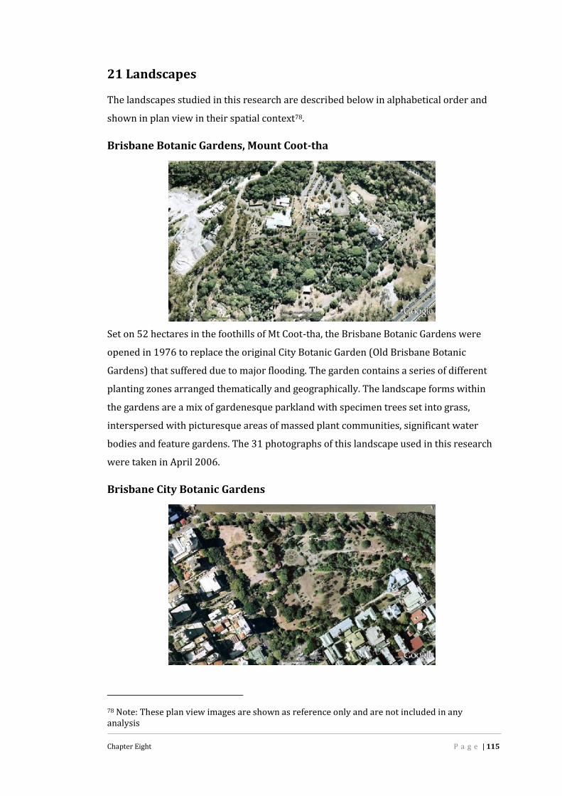
Chapter Eight P a g e | 115
21 LandscapesThe landscapes studied in this research are described below in alphabetical order andshown in plan view in their spatial context78.Brisbane Botanic Gardens, Mount Coot-tha
Set on 52 hectares in the foothills of Mt Coot-tha, the Brisbane Botanic Gardens wereopened in 1976 to replace the original City Botanic Garden (Old Brisbane BotanicGardens) that suffered due to major flooding. The garden contains a series of differentplanting zones arranged thematically and geographically. The landscape forms withinthe gardens are a mix of gardenesque parkland with specimen trees set into grass,interspersed with picturesque areas of massed plant communities, significant waterbodies and feature gardens. The 31 photographs of this landscape used in this researchwere taken in April 2006.Brisbane City Botanic Gardens
78 Note: These plan view images are shown as reference only and are not included in anyanalysis

Chapter Eight P a g e | 116
Brisbane City Botanic Gardens, adjacent to the Brisbane River, were laid out by WalterHill from 1855. It is now considered to be “a living museum of plant collections,displaying early heritage specimens through to present day exotic and nativeplantings”79. The gardens are laid out with linear paved paths lined with trees, spaciousgardenesque style lawn areas dotted with specimen trees, geometric water featuresand both linear and curvilinear horticultural garden beds. The 32 photographs of thislandscape used in this research were taken in April 2006.Brisbane CBD
Brisbane City Centre is a growing modern central city streetscape of high-rise offices,apartments, shops, traffic and street vegetation. The majority of the city centre is basedon an orthogonal street pattern. The 72 photographs of this landscape used in thisresearch were taken in March 2006.Cambridge City Centre, UK
Cambridge is an historic English market city and the home of Cambridge University.The City contains a mix of ancient university buildings that date from 1284 and modern79 http://www.brisbanehistory.com/botanical_gardens.htm, accessed 28 September 2010

Chapter Eight P a g e | 117
architectural forms. As can be seen in the aerial image above, all these buildings are setwithin a non-orthogonal medieval street pattern. Although surrounded by parks thatborder the River Cam, the City centre contains very little vegetation except that withinthe University Colleges. The dominant architectural form is that of low rise Neo-Gothicand Georgian with significant surface detail. The 41 photographs of this landscape usedin this research were taken in February 2008.Chermside Hills Reserve
The Chermside Hills area was declared a Reserve in 1972 and has an area of 116hectares. The Reserve contains a mix of relatively undisturbed coastal heathland, openEucalypt woodland and riparian vegetation. It forms part of Brisbane City Council’s‘Mountains to Mangroves’ corridor80. The Reserve contains a network of low impactunpaved trails and is surrounded by developed residential land. The 75 photographs ofthis landscape used in this research were taken in March 2006.Childers Farm Land
80 See http://www.brisbane.qld.gov.au/documents/environment/chermside_hills_brochure.pdf,accessed September 2010.

Chapter Eight P a g e | 118
The farm land that surrounds the regional Queensland town of Childers is composed ofa mix of cattle, dairy and arable farms, such as sugar cane and macadamia nutplantations, on red basaltic soil. The 36 photographs of this landscape used in thisresearch were taken in 2006.Childers Town Centre
Childers is an historic regional town that dates from the 1850s. Developed to serve thesurrounding agricultural properties it is still a major economic hub in the Wide Bayregion. The town is split by the Bruce Highway, the major route north along the coastalQueensland. The 52 photographs of this landscape used in this research were taken inAugust 2006.Childers is regarded as ‘...one of the most picturesque small towns in Queensland’81Dundowran Beach
Dundowran Beach is a predominantly wild-natural beachside environment formingpart of Hervey Bay and stretches for approximately 7km. Due to the shallow nature of81 See http://en.wikipedia.org/wiki/Childers,_Queensland , accessed September 2010

Chapter Eight P a g e | 119
the bay, Dundowran Beach has a very large inter-tidal zone that supports an abundanceof bird and other wildlife. The adjacent dune vegetation consist of a rich upper storeycontaining tree species such as: Casuarina equisetifolia, Callitris colomellaris, Hibiscus
tiliaceus, Corymbia tessellaris, Ficus virens, Flindersia bennetiana, Banksia integrifolia,Alphitonia excelsa, Planchonia careya, Cupaniopsis anacardioides, Melaleuca
quinquenervia, Melaleuca dealbata, Pandanus tectorius, Agathis robusta and Acacia sp.The 49 photographs of this landscape used in this research were taken betweenDecember 2007 and December 2008Green Park, London
Green Park is one of four Royal Parks in London and is set on 19 hectares adjacent toBuckingham Palace. Originally a deer park created by Charles II in 1688, it nowcontains mature Plane (Platanus sp) and Lime (Tilia sp) trees set in a grid-like patternwithin a grassland setting and criss-crossed by gravel walks. The 23 photographs ofthis landscape used in this research were taken in February 2008.Hervey Bay Botanic Gardens

Chapter Eight P a g e | 120
Hervey Bay Botanic Gardens have been developing since 1974. At present there is adistinct boundary between the formal planned gardens and the bordering, relativelyuntouched, Beach Ridge Open Forest (Landplan 2007, 58). These two areas areconsidered separately.Part APart A of the gardens contains the constructed section that began in 1974 and containsplanting beds that represent a variety of plant communities within the Fraser Coastregion. The area also contains a lake and several interlinked walkways. The 37photographs of this landscape used in this research were taken in September 2006.Part BPart B of the gardens contains some of the relatively untouched remnants of theoriginal Beach Ridge Open Forest (Landplan 2007). The 33 photographs of thislandscape used in this research were taken in September 2006.Hervey Bay Esplanade
The Hervey Bay Esplanade is a major tourist environment within the Wide Bay regionof South East Queensland and is characterised by its low-rise residential andcommercial development on the southern and its remnant vegetated foreshore on thenorthern side. The foreshore has a paved path that runs the full length of the Esplanadethat is a popular walking, running and cycle path. The 58 photographs of this landscapeused in this research were taken in August 2006.

Chapter Eight P a g e | 121
London, EC1
These photographs record a random walk through the streets of East London and partof the City of London, in a south-easterly direction, from St Pancras Station to St Paul’sCathedral, via Cambden, Clerkenwell, Holborn and St Bartholomew’s Hospital. This areacontains many Victorian and Georgian buildings intermixed with more modernarchitecture. Vegetation is limited to the few public parks and squares such a Coram’sFields, Mecklenburg Square and Northampton Square, while street trees are minimal.The land use vary from residential to commercial with more office space as youappraoch St Paul’s and the City of London business district. The 57 photographs of thelandscape used in this research were taken in February 2008.London, W1
These photographs record a random walk through the streets of West London in asouth-westerly direction, from St Pancreas Station to Marylebone High Street, via theBritish Library, Cartwright Gardens, Russell Square and Broadcasting House. Similar toEast London, this area contains an historic mix of Victorian and Georgian buildingsinterspersed with modern architecture. Building use is predominantly residential andcommercial. Vegetation is limited to public parks and squares with very limited use of

Chapter Eight P a g e | 122
street trees. The 91 photographs of this landscape used in this research were taken inFebruary 2008.Melbourne Docklands
Photographed: May 2009Docklands is set on approximately 200 hectares of land and water and includes sevenkilometres of waterfront. The urban design for this development divided the area intoprecincts, each with their own distinct visual character and they include a mix ofresidential, retail and commercial activities. Staged development of this area began inthe 1990s and the final stages of construction are due to finish around 2020. Then,Docklands will double the size of the existing Melbourne CBD82. The 38 photographs ofthis landscape used in this research were taken in May 2009.Regent’s Park, London
Originally designed by John Nash around 1811 and set on 149 hectares, this parkencompasses a mix of Victorian style gardens, including geometric avenues, flower82http://www.docklands.com/cs/Satellite?c=VPage&cid=1182477286483&pagename=VicUrban%2FLayout&site=Docklands, accessed 28 September 2010

Chapter Eight P a g e | 123
beds, rose gardens and a lake. The park also contains the largest outdoor sports area inCentral London. Today, ‘...it has assumed the role of the old pleasure-gardens with itsbandstand and open-air theatre’ (Symes 2001). The 57 photographs of this landscapeused in this research were taken in February 2008.Roma Street Parkland
The Roma Street Parkland was developed on former railway land that adjoined theexisting Albert Park, with which it is now integrated. The park opened to the public inApril 2001. The planting within the park has been developed as distinct precincts,“...creating the feel of a subtropical wonderland representing Queensland’s varied plantlife83. These precincts are linked by both water and walkways. Sculptures and other artworks provide additional the visual stimulation and provide a link to the heritage of theParkland with its current natural and urban surrounds. The 96 photographs of thislandscape used in this research were taken in September 2008.Royal Botanic Gardens Cranbourne
83 http://www.romastreetparkland.com/aboutus/Pages/design.aspx, accessed September 2010

Chapter Eight P a g e | 124
These gardens contain 363 hectares of native bushland. The section of gardensphotographed for this study is limited to the designed Australian Garden (Stage 1)opened in May 2006. The Australian Garden is an award winning landscape ofAustralian flora, art and architecture. The garden features a series of display andsculpture gardens that focus on the diversity of the Australian landscape. The 58photographs of this landscape used in this research were taken in May 2009.South Bank Parklands
These parklands, directly opposite the city centre on the south bank of the BrisbaneRiver, were built on the site of the World Expo 88. The parklands, which were openedto the public in 1992, contain a mixture of garden beds, rainforest plantings, waterfeatures, spacious lawn areas and plazas. The parklands are also well known for theirriverfront promenade, the public beach pool and the steel and bougainvillaea coveredGrand Arbour. The area surrounding the parklands is now home to many restaurantsand shops. The 76 photographs of this landscape used in this research were taken inSeptember 2009.St James’ Park, London

Chapter Eight P a g e | 125
Set in the heart of London on 23 hectares, St James’s Park is the oldest of the four RoyalParks and is surrounded by three palaces―Westminster Palace (now the Houses ofParliament), St James’s Palace and Buckingham Palace. The park was first laid out forCharles II by André Mollet in 1660 and remodelled by John Nash in the reign of GeorgeIV (1820―30). The park now contains mature trees set in spacious lawn areas with acentral lake and is criss-crossed by a number of paths. The 22 photographs of thislandscape used in this research were taken in February 2008.Toowoomba City Centre
Photographed: June 2006Dating back to 1827, Toowoomba is located about 127km west of Brisbane. It sits onthe edge of the Great Dividing Range escarpment about 700m above sea level. It is themajor commercial and economic centre for the Darling Downs agricultural area and isone of the largest inland regional cities in Australia. The city centre is characterised bylow-rise buildings and wide paved streets. The 51 photographs of this landscape usedin this research were taken in June 2006.Research Question One
Do different landscape forms, ranging from relatively natural to highlyurban show a variation in their overall fractal dimension?As discussed in Chapter 4, any environments that are created and sustained by primaryenergy are considered to be Natural environments84 , while any environments thatrequire the power of secondary energy for their creation and maintenance areconsidered Para-natural environments. It is also clear that all Para-naturalenvironments require Natural elements and processes for their creation and many
84 See Chapter 4 for a discussion on the use of secondary energy by some natural entities.

Chapter Eight P a g e | 126
require some Natural elements and processes to sustain delivery of their designedfunction/purpose. Therefore, Research Question One can now be re-phrased as:Do different landscape forms ranging from Wild Nature to ConstructedNature show a variation in their overall fractal dimension?
Fractal AnalysisThe complete results of the fractal analysis for each of the digital images made for thelandscapes described in Chapter 6 are documented in Appendix C, Section 1.Table 8.1 presents a summary of this data, wherein D2 is the median two-dimensionalfractal dimension for each landscape.Table 8. 1: Landscape Fractal Analysis Summary
Landscape Id MedianVegetationRating
Number ofImages
Median D2 MedianR2X
MedianR2Y
Brisbane Botanic Gardens BBG 5 32 2.567 0.612 0.567
Brisbane City BotanicGardens
BCBG 5 32 2.513 0.644 0.585
Cambridge, UK85 CB 1 41 2.451 0.667 0.663Central Brisbane City CBC 2 72 2.418 0.663 0.656Chermside Hills Reserve CHR 5 75 2.567 0.594 0.555
Childers Farm Land CFL 4 36 2.558 0.691 0.477Childers Town Centre CTC 3 52 2.483 0.659 0.598Cranbourne BotanicGardens
CBG 3 58 2.470 0.670 0.605
Dundowran Beach DB 2 49 2.489 0.670 0.607
Green Park, London UK GP 5 23 2.591 0.588 0.563Hervey Bay BotanicGardens - A
HBBGa 5 37 2.540 0.612 0.586
Hervey Bay BotanicGardens - B
HBBGb 5 33 2.579 0.594 0.577
Hervey Bay Esplanade HBE 4 58 2.476 0.654 0.618London East Central, UK LEC 1 57 2.491 0.649 0.603
London West One, UK LW 1 91 2.415 0.667 0.653Melbourne Dock Lands MD 1 38 2.413 0.682 0.640Regents Park, London UK RP 4 57 2.614 0.588 0.534
Roma Street Parklands RSP 4 96 2.505 0.622 0.597South Bank Parklands SBP 3 76 2.488 0.643 0.613St James Park, London UK StJP 5 22 2.602 0.582 0.533
Toowoomba City Centre TCC 2 51 2.458 0.675 0.602
Figure 8.1 shows a Box Plot that compares the median and the range of fractaldimensions for images of the different landscapes. It can be seen that the fractal85 On the day the photographs were taken the City was covered in a light mist that gives a ‘soft’look to all the images.

Chapter Eight P a g e | 127
dimension across all landscapes studied shows a distinct variation between 2.000 and3.000. The line across the box86 is the median value for that landscape.Recalling the explanation in Chapter 6, a photographic image is considered to have atopological dimension of two (2). Therefore, these results show that each imageexhibits a level of statistical self-similarity that generates a fractal dimension for thatimage that exceeds its topological dimension. These results are consistent with thediscussion on fractal geometry in Chapter 5 that shows a fractal two-dimensional planewill exhibit a fractal dimension between two (2) and three (3).
Figure 8. 1: Box Plot for Overall Fractal Dimension DataHowever, what is also evident from these results is that images from differentlandscape forms can display the same fractal dimension. This is a statistically validresult and will be discussed in Research Question 2.Data ValidityFigure 8.2 graphs the median R2 values for the one dimensional X and Y fractaldimension for each landscape. The R2 statistic, called the Coefficient of Determination,is a measure of how well the model fits the actual data. The closer the value is to one (1)the better the fit. It can be seen that the majority of the data trends around the 0.600level. This indicates that the fit of the model to the data was similar for all landscapesstudied. The one value that is outside the general trend is the R2Y value for Childersfarm land.
86 This represents the middle 50% of values.

Chapter Eight P a g e | 128
Figure 8. 2: Median R2 Values for Landscape vs. Fractal DimensionIn Figure 8.3, shows the distribution of the overall median fractal dimension for eachlandscape, ranked in a hierarchy from lowest to highest. The Vegetation Rating for eachlandscape is also presented.
Figure 8. 3: Variation in Median Fractal DimensionThe linear trend line shown in Figure 8.3 is derived by linear regression analysis inMicrosoft Excel. It can be seen from the R2 value for this analysis that there is a close fitbetween the regression line and the data. This indicates that there is a trend for the
different landscapes studied to display different median fractal dimensions.
However, it can also be seen that the landscapes that have been assessed as beingclosest to Wild Nature ―Chermside Hills Reserve, Dundowran Beach and Hervey BayBotanic Gardens-Part B―were not ranked the highest. These results will be discussedfurther in Chapter 9.

Chapter Eight P a g e | 129
Research Question Two
Is there a statistically significant difference between the Fractaldimensions of commonly encountered landscape forms?To answer this question it was initially hypothesised that all landscapes studied willhave the same median fractal dimension, as a baseline from which to begin the analysis.To test this hypothesis, an Analysis of Variance (ANOVA) test with a 95 per centsignificance level was performed on the fractal dimensions for all images across alllandscapes. The results of this analysis are shown in Table 8.2.
Table 8. 2: ANOVA Results for Fractal Dimension vs Landscape
Estimate Std. Error t value Pr(>|t|) SignificanceIntercept 2.547483 0.011177 227.921 < 2e-16 5
LandscapeBCBG -0.049915 0.015807 -3.158 0.001634 4CB -0.083148 0.015081 -5.513 4.41E-08 5CBC -0.138122 0.013433 -10.282 < 2e-16 5CBG -0.083346 0.013881 -6.004 2.63E-09 5CFL 0.001644 0.015361 0.107 0.914778 1CHR 0.015059 0.01335 1.128 0.259564 1CTC -0.057806 0.014206 -4.069 5.07E-05 5DB -0.053018 0.014371 -3.689 0.000236 5GP 0.03298 0.017073 1.932 0.053667 2HBBGa -0.011956 0.015263 -0.783 0.43363 1HBBGb 0.024049 0.015687 1.533 0.125542 1HBE -0.070287 0.013923 -5.048 5.24E-07 5LEC -0.049084 0.013881 -3.536 0.000424 5LW -0.127954 0.012976 -9.861 < 2e-16 5MD -0.127272 0.015263 -8.338 2.30E-16 5RP 0.062443 0.013923 4.485 8.09E-06 5RSP -0.046713 0.012906 -3.619 0.000309 5SBP -0.064812 0.013324 -4.864 1.32E-06 5StJP 0.038558 0.017511 2.202 0.027884 3TCC -0.095469 0.014259 -6.695 3.47E-11 5
SignificanceCodes
5 = 0 4 = 0.001 3 = 0.01 2 = 0.05 1 = 0.1
Residual standard error: 0.06323 on 1068 degrees of freedomMultiple R-squared: 0.4429, Adjusted R-squared: 0.4325F-statistic: 42.45 on 20 and 1068 DFP < 2.20e-16
The P < 0.22e-15 result provides strong evidence for rejecting this hypothesis. However,to ensure that the results of the ANOVA are not due to chance as a result of multiple

Chapter Eight P a g e | 130
comparison errors, a Tukey’s honest significance difference test with a 95 per centconfidence interval was applied to the data (Reeves 2006). This test compares themedian fractal dimension between every possible pair of landscapes, accounting formultiple comparisons, and determines which landscapes are significantly differentfrom each other and which are not. The results of this test are further documented inAppendix D, Section 1. This analysis shows that of the 210 unique comparisons
between fractal dimensions, 128, or approximately 61 percent, were considered
significantly different.
The fact that the overall fractal dimensions for each landscape were not all significantlydifferent from each other is not surprising, as it should be expected that similarlandscape forms will have a similar median fractal dimension. For example, the resultsshow that Chermside Hills Reserve and Hervey Bay Botanic Gardens-Part B, bothassessed as being close to Wild Nature and both with a Vegetation Rating of 5, are notsignificantly different based on their median fractal dimensions. Similarly, BrisbaneCBD and London West One, which have a Vegetation Rating of 1, are also notsignificantly different.However, the analysis also shows that the median fractal dimensions for Cambridge, UKwith a Vegetation Rating of 1 and Brisbane City Botanic Gardens with a VegetationRating of 5 are not significantly different. Similarly, London East Central with aVegetation Rating of 1 and Dundowran Beach with a Vegetation Rating of 2 are also notsignificantly different. These seemingly contradictory findings do not mean that each ofthese disparate landscapes is identical; rather, that there is not enough statisticalevidence for the Tukey HSD test to show that they are different (Lane et al. 2011).The results show that individual images from very different landscapes can
produce the same or very similar fractal dimensions. This is an important finding iffractal geometry is to play a role in design and will be discussed in more detail inChapter 9.

Chapter Eight P a g e | 131
Research Question Three
Can the fractal properties of a landscape be considered as a measure ofits ‘naturalness’87?To determine whether the fractal dimension can be considered as a measure ofnaturalness, the overall median two-dimensional fractal dimension of a landscape iscompared to the overall median Vegetation Rating for that landscape. The VegetationRating is determined as per the method outlined in Chapter 7. The full results of thisare shown in Appendix B. From these results, a median Vegetation Rating for aparticular landscape is calculated. These results are shown in Table 8.3 below, rankedfrom lowest to highest.
Table 8. 3: Vegetation Rating
Landscape Vegetation RatingLondon East Central, UK 1Cambridge, UK 1Melbourne Docklands, Victoria, Aus 1London West One, UK 1Dundowran Beach, Queensland, Aus 2Toowoomba City Centre, Queensland, Aus 2Central Brisbane City, Queensland, Aus 2South Bank Parklands, Brisbane, Queensland, Aus 3Childers Town Centre, Queensland, Aus 3Cranbourne Botanic Gardens, Victoria, Aus 3Regents, Park, London, UK 4Childers Farm Land, Queensland, Aus 4Roma Street Parkland, Queensland, Aus 4Hervey Bay Esplanade, Queensland, Aus 4St James Park, London, UK 5Green Park, London, UK 5Hervey Bay Botanic Garden –Part B, Queensland, Aus 5Chermside Hills Reserve, Queensland, Aus 5Brisbane Botanic Gardens, Queensland, Aus 5Hervey Bay Botanic Garden –Part A, Queensland, Aus 5Brisbane City Botanic Gardens, Queensland, Aus 5
Fractal Dimension as a Measure of NaturalnessThe overall median fractal dimension for each of the landscapes and their VegetationRatings are shown in Figure 8.4 below.87 The concept of ‘naturalness’ is discussed in Chapters 4 and 7. However, when this questionwas originally formulated, the concept of a ‘fractal property’ had not been defined in any greatdetail and was based on a limited understanding of fractal geometry. It is now clear that the onlyobjective fractal property determined through this work is that of the Fractal dimension.

Chapter Eight P a g e | 132
It can be seen from this graph that all landscapes with a median fractal dimensionabove 2.491 (the overall median value) have a Vegetation Rating of either 4 or 5.Therefore, if we accept the premise that the level of vegetation is indicative ofnaturalness, then the fractal dimension can be also be considered an indicator ofnaturalness. However, there are two exceptions to this that negate this premise andrequire further discussion. These landscapes are Dundowran Beach and London EastCentral.
Figure 8. 4: Vegetation Ratings vs. Landscape
Dundowran BeachDundowran Beach is a landscape form that is almost untouched by Para-naturalprocesses and elements and therefore is very close to Wild Nature. It has a medianfractal dimension of 2.489, which is slightly lower that the overall median value for alllandscapes and a Vegetation Rating of 2. An examination of the images for thislandscape show that the statistically self-similar patterns created within this landscapeare clearly a result of Natural processes at work. Examples of this are shown in Figure8.5.However, at the scale of observation used, these patterns have tended to produce alower level of measured fractal dimension than the patterns produced by vegetation inother landscapes.
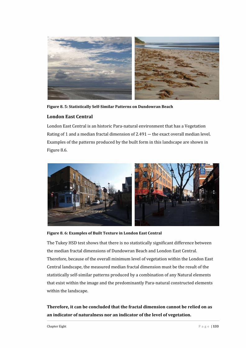
Chapter Eight P a g e | 133
Figure 8. 5: Statistically Self-Similar Patterns on Dundowran Beach
London East CentralLondon East Central is an historic Para-natural environment that has a VegetationRating of 1 and a median fractal dimension of 2.491 ― the exact overall median level.Examples of the patterns produced by the built form in this landscape are shown inFigure 8.6.
Figure 8. 6: Examples of Built Texture in London East CentralThe Tukey HSD test shows that there is no statistically significant difference betweenthe median fractal dimensions of Dundowran Beach and London East Central.Therefore, because of the overall minimum level of vegetation within the London EastCentral landscape, the measured median fractal dimension must be the result of thestatistically self-similar patterns produced by a combination of any Natural elementsthat exist within the image and the predominantly Para-natural constructed elementswithin the landscape.Therefore, it can be concluded that the fractal dimension cannot be relied on as
an indicator of naturalness nor an indicator of the level of vegetation.

Chapter Eight P a g e | 134
Research Question Four
Does the use of re-iterated forms at different scales affect the fractaldimension of a landscape?The concept of re-iterated form is embodied in the exactly self-similar mathematicalfractals patterns discussed in Chapter 5. These forms represent a pattern wherein theshape of the pattern is repeated at all scales of observation. Although re-iterated formhas been used, in a limited way, in architecture during earlier epochs88, the use of thisform as an intentional device to manipulate the fractal dimension of a designedlandscape is limited by the plane of observation and the range of scales at which adesign landscape is experienced.
One of the few modern landscapes that has experimented with self-similar fractal formsis the Garden of Cosmic Speculation designed by Charles Jenks and his wife MaggieKeswick, at Portrack, Dumfriesshire in Scotland (Turner 2010). This Garden uses staticconstructed forms to represent the underlying Natural processes that reverberatethroughout the cosmos; from the structure of DNA and the waveforms of strangeattractors in Chaos Theory and Soliton Waves to large structures such as the UniverseCascade, which tries to represent the history of the universe (Jencks 2003).There is no doubt that like all great gardens Jenck’s Garden of Cosmic Speculationprovokes very different responses in different people. Tim Richardson (2007)considers this garden to be neither symbolic nor conceptual, but a demonstrationgarden where “features are created in order to replicate physical expressions ofcosmological theory in a highly literal manner, in the way of those little red moleculeballs connected by sticks, so beloved of chemistry teachers”. Richardson feels that thegarden is no longer in a dialogue with the universe but has become a monologue and isbecoming “The Garden of Comic Extrapolation”. In contrast, Tom Turner (2010) would“congratulate Jencks for taking the historic trajectory of landscape design theoryforward in a way which most landscape architects have failed to do”.There are many similarities between this garden and the gardens of the 18th century,such as Stowe in Buckinghamshire, England. Both gardens require significant cognitiveunderstanding of the underlying philosophy and symbolism embedded in the design tofully appreciate the designer’s intent. But both gardens can also be considered as88 See Chapter 4
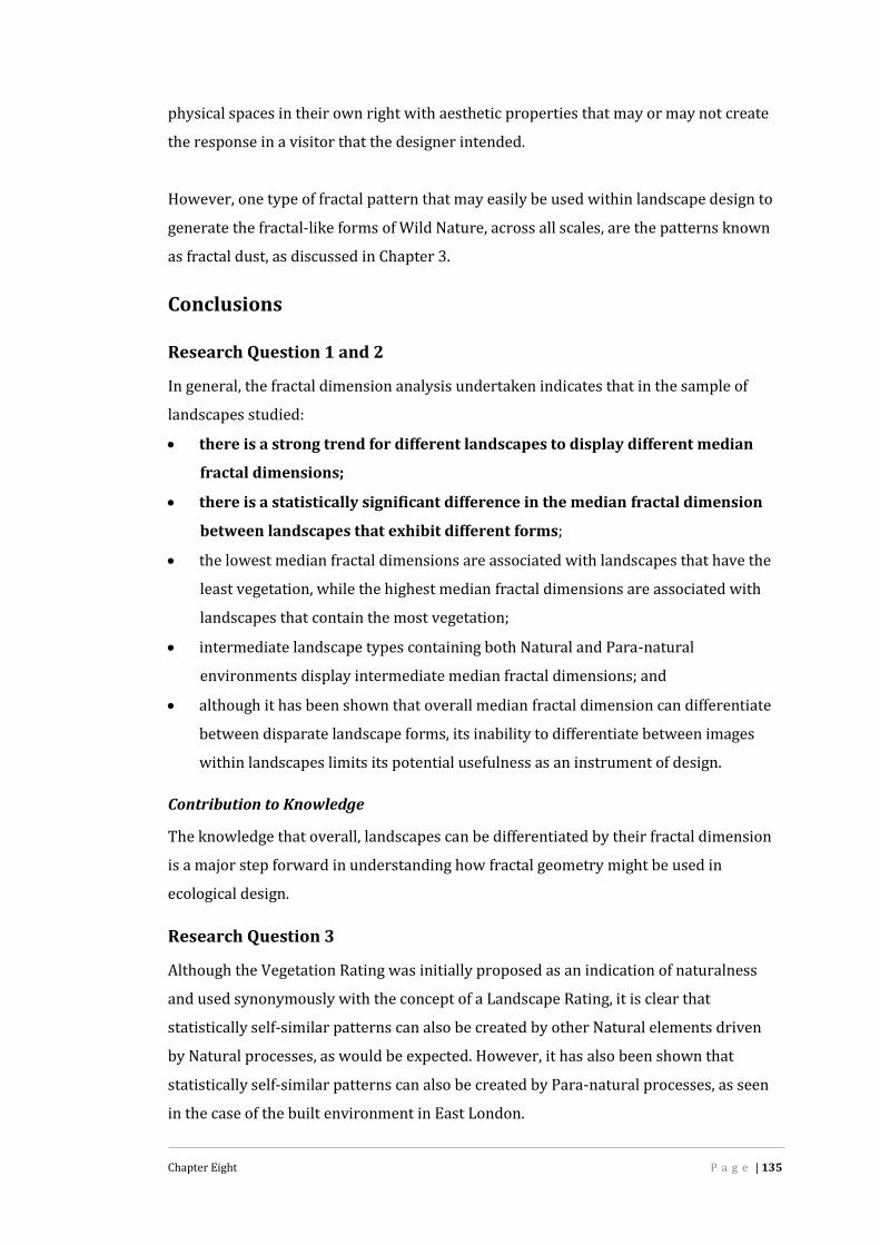
Chapter Eight P a g e | 135
physical spaces in their own right with aesthetic properties that may or may not createthe response in a visitor that the designer intended.However, one type of fractal pattern that may easily be used within landscape design togenerate the fractal-like forms of Wild Nature, across all scales, are the patterns knownas fractal dust, as discussed in Chapter 3.Conclusions
Research Question 1 and 2In general, the fractal dimension analysis undertaken indicates that in the sample oflandscapes studied: there is a strong trend for different landscapes to display different median
fractal dimensions;
there is a statistically significant difference in the median fractal dimension
between landscapes that exhibit different forms; the lowest median fractal dimensions are associated with landscapes that have theleast vegetation, while the highest median fractal dimensions are associated withlandscapes that contain the most vegetation; intermediate landscape types containing both Natural and Para-naturalenvironments display intermediate median fractal dimensions; and although it has been shown that overall median fractal dimension can differentiatebetween disparate landscape forms, its inability to differentiate between imageswithin landscapes limits its potential usefulness as an instrument of design.Contribution to KnowledgeThe knowledge that overall, landscapes can be differentiated by their fractal dimensionis a major step forward in understanding how fractal geometry might be used inecological design.Research Question 3Although the Vegetation Rating was initially proposed as an indication of naturalnessand used synonymously with the concept of a Landscape Rating, it is clear thatstatistically self-similar patterns can also be created by other Natural elements drivenby Natural processes, as would be expected. However, it has also been shown thatstatistically self-similar patterns can also be created by Para-natural processes, as seenin the case of the built environment in East London.

Chapter Eight P a g e | 136
Contribution to Knowledge
This finding is very significant for design, as it implies that a particular design formand its content will have a significant impact on the overall fractal dimension of alandscape at the normal scales of observation.Research Question 4The conscious use of re-iterated exact self-similar form in landscape design would berelatively simple to achieve through the design of geometric shapes that arereflectaphoric in both positive and negative space. However, what this thesis hasshown is that the influence on the overall fractal dimension of a landscape throughusing re-iterated design forms is impossible to predict.From the discussions in preceding chapters it can be seen that the overall fractaldimension will be dependent on the ratio of Natural and Para-natural environments,the type of materials in the landscape and the scale at which the landscape isexperienced. A more likely outcome of the use of re-iterated form, at the overalllandscape scale, would be to create a feeling of underlying unity within the landscape inthe same way that reflectaphors have been proposed as a device to unify a work of art.Contribution to KnowledgeThis knowledge is very significant, as it provides a theoretical understanding for theuse of re-iterated fractal form within landscape design practice.Beyond the Fractal DimensionIn the past, overall landscapes have been classified by land use or function rather thanform. This is evident in established planning language that uses terms such as rural,sub-urban, urban, business, commercial, industrial, open space or recreational. Eventhe term National Park is a function based terminology. This research has shown thatthe fractal dimension can provide a measurable parameter that can distinguishbetween overall landscape forms based on structural content.However, although Natural environments have, in general, been shown to exhibit ahigher fractal dimension than Para-natural environments, it has also been shown thatsome Para-natural environments can exhibit a fractal dimension similar to or greaterthan Natural environments. Also, the examples of Dundowran Beach and London EastCentral show that the fractal dimension is only a measure of the statistical self-similarity of the patterns encoded within a particular image of a landscape and within

Chapter Eight P a g e | 137
the whole set of images collected to represent that landscape. This result is veryimportant as it implies that once this patterning is understood, a landscape can beconsciously designed to exhibit the same range of fractal dimensions that are present inNatural environments.Fractal Dimension and Landscape FormThe fractal dimension, as computed in this research, is a measure of the statistical self-similarity of a landscape encoded within a digital image and also within anenvironment as a whole. But the question remains as to how this relates to the visiblelandscape form. As discussed in Chapter 6, the fractal dimension of a landscape iscomputed from the power spectrum derived from the underlying structural geometryof the landscape image. The frequencies within the power spectrum are computed fromthe pixel luminance values. As shown diagrammatically in Chapter 6, the amplitude ofthe component frequencies tends to decrease exponentially with the log of frequency.The greater the level of fine detail within the image the greater the number of higherthe frequency components and hence the greater the degree of self-similarity (Russ2007, 355). How this is represented in the structure of a landscape is demonstrated inFigure 8.7 and Figure 8.8 for more natural environments and in Figures 8.9 and 8.10 forurban environments.
Figure 8. 7: Image GP20 Row AnalysisFigure 8.7 shows image GP20 from Green Park, London. The highlighted rows crossvarious degrees of structural detail within the image at different perspective distances.Row 200 crosses the open structure of the bare tree branches, Row 900 crosses thealmost solid structure of the background trees and Row 1820 crosses the fine texture of

Chapter Eight P a g e | 138
the foreground grass. Figure 8.8 shows the one dimensional power spectrum and theresultant fractal dimension associated with these rows.
Figure 8. 8: One Dimensional Power Spectrums for Figure 8.7As can be seen in Figure 8.8, Row 182,0 which crosses the fine grass texture seen in theforeground, has the highest fractal dimension. Row 200, which crosses the dense opentree branches in the mid-ground, has a fractal dimension just slightly lower and Row900, which crosses the almost solid structure of the trees in the distance, has thelowest.
Figure 8. 9: Image LW2 Row AnalysisFigure 8.9 shows image LW2 of the British Library from West London. As for the imagefrom Green Park, the highlighted rows cross various degrees of structural detail withinthe image as seen at different perspective distances within the image. Row 1270crosses the fine structure of the building brickwork seen at a the middle distance, Row1675 crosses the smooth structure of the concrete edge surrounding the raised gardenseen in the foreground and Row 1750 crosses the more open structure of the building

Chapter Eight P a g e | 139
brickwork also seen in the foreground. Figure 8.10 shows the one dimensional powerspectrum and the resultant fractal dimension associated with these rows.
Figure 8. 10: One Dimensional Power Spectrums for Figure 8.9As can be seen, Row 1270, which crosses the building brickwork seen at a distance, hasthe highest fractal dimension. Row 1750, which crosses the building brickwork seen inthe foreground, has the next lowest and Row 1675, which crosses the smooth concreteedge has the lowest.This analysis demonstrates that the fractal dimension, as computed, is dependent onthe relative amplitudes of the frequencies in the power spectrum rather than theabsolute values. It also highlights that the fractal dimension of an element within alandscape, or even the complete landscape, is dependent on the scale at which it isobserved. Therefore, the fractal pattern created by any particular element, orlandscape, must be considered as a dynamic property of that element or landscapelinked to movement through a landscape. Consequently, to understand and applyfractal geometric properties as a design tool it is essential to consider the detailedstructural form of the component elements, their surface textures and the scales atwhich they will be generally observed.Overall Conclusions to Research QuestionsMandelbrot associated fractal Geometry with Nature, however, it is clear in his book(1983) that his conception of nature was more aligned to the concept of Wild Naturediscussed in Chapter 4. What this work has shown is that fractal geometry and themeasurement of the fractal dimension in particular, can be used to differentiatecomplex three-dimensional real world landscapes comprised of both Natural and Para-natural environments. As discussed, this result aligns with the proposition by CatherinBull (1996, 27) that Nature (in its totality) is the content of landscape design.

Chapter Eight P a g e | 140
In their paper examining the validity of power laws89, for estimating the self-similarityfor natural systems, Avnir et al (1998) conclude that “fractal geometry provides aproper language and symbolism for studies of ill-defined geometries.” This is supportedby the results of this research that found the fractal dimension to be a gooddifferentiator of landscape type.However, although statistically valid, it has been found that many images from differentlandscape types exhibit the same or very similar fractal dimensions. Therefore, asdetailed landscape design does not generally occur at the broad scale encompassed bythe set of images that represent each landscape studied, the fractal dimension alonecannot be used in isolations as a design parameter. Consequently, further analysis ofthe individual images within each landscape is now required to determine whetherthere are other embedded properties, associated with the underlying geometricstructure of a landscape, which can be articulated and developed for use in a designcontext. This is discussed further in the Chapter 9.
89 Chapter 3 discusses the power law basis for fractal geometry

Chapter Nine P a g e | 141
Chapter Nine
The Geometric Properties of Landscapes
Failure to appreciate the dynamic autonomous role of nonhumanfeatures and phenomena promotes the illusion that humans can
construct and control everything. (Spirn 1996, 112)
IntroductionAlthough it has been revealed that different landscapes forms display different overallmedian fractal dimensions, the results of the fractal analysis on all images from thelandscapes studied has shown that images from very different landscape can have verysimilar fractal dimensions. This is illustrated by the images within each pair in Figure9.1. Here the fractal dimension is shown to three significant figures.
Central Brisbane City, Image 4Vegetation Rating = 1
Fractal Dimension = 2.516
Chermside Hills Reserve, Image 53Vegetation Rating = 5
Fractal Dimension = 2.516
London West One, Image 71Vegetation Rating = 1
Fractal Dimension = 2.384
Dundowran Beach, Image 50Vegetation Rating = 1
Fractal Dimension = 2.384
Figure 9. 1: Pairs of Images with Identical Fractal Dimensions (to 3 significant figures)
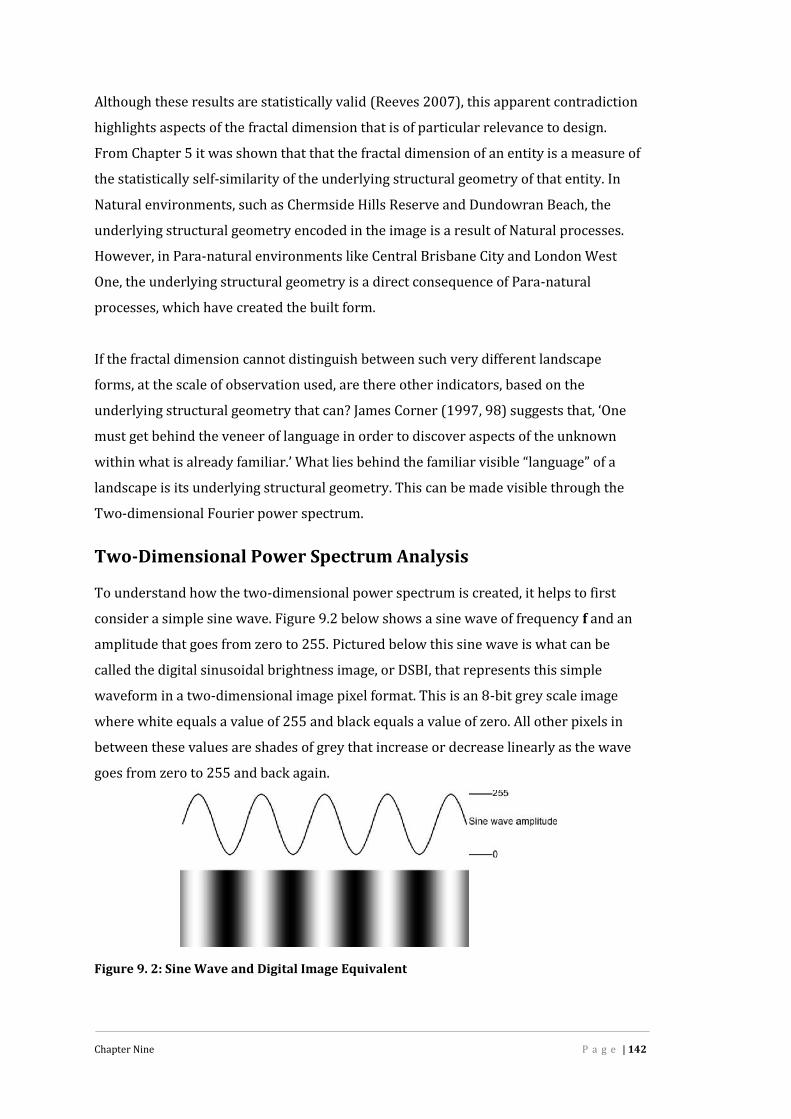
Chapter Nine P a g e | 142
Although these results are statistically valid (Reeves 2007), this apparent contradictionhighlights aspects of the fractal dimension that is of particular relevance to design.From Chapter 5 it was shown that that the fractal dimension of an entity is a measure ofthe statistically self-similarity of the underlying structural geometry of that entity. InNatural environments, such as Chermside Hills Reserve and Dundowran Beach, theunderlying structural geometry encoded in the image is a result of Natural processes.However, in Para-natural environments like Central Brisbane City and London WestOne, the underlying structural geometry is a direct consequence of Para-naturalprocesses, which have created the built form.If the fractal dimension cannot distinguish between such very different landscapeforms, at the scale of observation used, are there other indicators, based on theunderlying structural geometry that can? James Corner (1997, 98) suggests that, ‘Onemust get behind the veneer of language in order to discover aspects of the unknownwithin what is already familiar.’ What lies behind the familiar visible “language” of alandscape is its underlying structural geometry. This can be made visible through theTwo-dimensional Fourier power spectrum.Two-Dimensional Power Spectrum AnalysisTo understand how the two-dimensional power spectrum is created, it helps to firstconsider a simple sine wave. Figure 9.2 below shows a sine wave of frequency f and anamplitude that goes from zero to 255. Pictured below this sine wave is what can becalled the digital sinusoidal brightness image, or DSBI, that represents this simplewaveform in a two-dimensional image pixel format. This is an 8-bit grey scale imagewhere white equals a value of 255 and black equals a value of zero. All other pixels inbetween these values are shades of grey that increase or decrease linearly as the wavegoes from zero to 255 and back again.
Figure 9. 2: Sine Wave and Digital Image Equivalent

Chapter Nine P a g e | 143
Single Spatial Frequency and the Fourier Power SpectrumThe DSBI in Figure 9.3 below represents a single sinusoidal frequency in the horizontalplane. The output of the Fourier Transform consists of two parts: the information thatcontains the phase of the frequency domain and the power spectrum90. The powerspectrum of the original DSBI is shown next to the original image. In the powerspectrum, the centre of the image represents the origin of the frequency co-ordinatesystems and each point represents a particular frequency contained in the spatialdomain image. It can be seen that the power spectrum for the DSBI contains threebright points on the x-axis. The central point is the co-ordinate origin called the zerofrequency, or DC point and it represents the average brightness of the image.
Original SBI of Frequency f Power Spectrum
Figure 9. 3: Two-Dimensional Power Spectrum of a Digital Sinusoidal Brightness ImageThe two points on either side of the DC point represent the frequency components ofthe DSBI. The distance of these points from the central DC point is proportional to thefrequency and the brightness (between 0 and 255) of the point is proportional to theamplitude of the frequency. This is shown in graphical form in figure 9.4.
Figure 9. 4: Two-dimensional Fourier Power Spectrum in Graphical Form
90 This research is only concerned with the power spectrum.

Chapter Nine P a g e | 144
It should be noted that there are two frequency points in the power spectrum, as theFourier Transform mirrors the result around the DC point.Figure 9.5 shows how the distance of the frequency points from the DC point increasesas the frequency of the sinusoidal brightness image increases.
Frequency DSBI Power Spectrum
f
2f
4f
8f
Figure 9. 5: Two-Dimensional Power Spectrum of Different Frequencies

Chapter Nine P a g e | 145
Orthogonal Spatial FrequenciesIf the original DSBI presents spatial frequencies that go in either the X or Y directionthen the frequency point will be on either axis of the power spectrum image ―recognizing that the Fourier Transform image is mirrored about the axis then quadrant1 = quadrant 3 and quadrant 2 = quadrant 4. This is shown in Figure 9.6 with equalfrequencies in both the horizontal and vertical planes.DSBI Power Spectrum
Figure 9. 6: Multiple Spatial Frequencies and the Power Spectrum
Angular Spatial FrequenciesIf the original spatial image also contains sinusoidal frequencies at an angle ofdegrees to the X axis, as shown in Figure 9.7, then the point on the power spectrumimage will be at an angle (90 − ) degrees and as before, the distance d from thecentre DC value will be proportional to the frequency.DSBI Power Spectrum
Figure 9. 7: Angular Sinusoidal Bright Frequencies and the Power Spectrum
This is shown graphically in Figure 9.8 below.

Chapter Nine P a g e | 146
Figure 9. 8: Angular Sinusoidal Brightness Images and their Power Spectrum
The Two Dimensional Power Spectrum of a Landscape ImageAs discussed in Chapter 6, the fractal dimension for each of the landscape images iscalculated from the one-dimensional power spectrum for each column and row ofpixels within the image. The advantage of the two-dimensional power spectrum of animage is that it is a representation of the underlying structural geometry of thelandscape form embedded within the image (Fisher et al. 2003). However, as explainedabove, when viewing the plots of a power spectrum, it must be remembered that theyare a reflected about the central point. This is shown in Figure 9.9, where it can be seenthat quadrant Q1 is reflected in Q3 and that quadrant Q2 is reflected in Q4.
Figure 9. 9: Two-Dimensional Power Spectrum StructureA review of the two-dimensional power spectrum for images from different landscapeforms provides an insight into how images from very different landscapes with similarfractal dimensions can be further differentiated. Figure 9.10 shows the power spectrum

Chapter Nine P a g e | 147
for the images in Figure 9.1. It can be seen that the power spectra from CentralBrisbane City and London West One display strong lines of energy radiating in a starpattern from the central DC point91, whereas, the power spectra for Chermside HillsReserve and Dundowran Beach do not exhibit these angular high energy lines92.
Central Brisbane CityTwo-dimensional p(f) for Image 4
Chermside Hills ReserveTwo-dimensional p(f) for Image 53
London West OneTwo-dimensional p(f) for Image 71
Dundowran BeachTwo-dimensional p(f) for Image 50
Figure 9. 10: Two-Dimensional Power Spectrum for Images with Similar FractalDimensions from Different Landscapes
The radiating lines of high energy in the power spectra for Central Brisbane City andLondon West One are due to the transitional ‘edge effect’ of the geometric built formswithin the landscape (Reeves 2009). These high energy lines are at 90 degrees to theelements within the image that are responsible for the effect. This is demonstrated inFigure 9.11 for an image from London East Central. The blue lines align with the91 Refer Chapter 692 The lines of varying brightness in the x and y axis directions within all images are a result ofthe underlying pixel image structure itself.
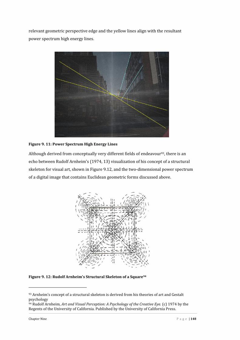
Chapter Nine P a g e | 148
relevant geometric perspective edge and the yellow lines align with the resultantpower spectrum high energy lines.
Figure 9. 11: Power Spectrum High Energy LinesAlthough derived from conceptually very different fields of endeavour93, there is anecho between Rudolf Arnheim’s (1974, 13) visualization of his concept of a structuralskeleton for visual art, shown in Figure 9.12, and the two-dimensional power spectrumof a digital image that contains Euclidean geometric forms discussed above.
Figure 9. 12: Rudolf Arnheim's Structural Skeleton of a Square94
93 Arnheim’s concept of a structural skeleton is derived from his theories of art and Gestaltpsychology94 Rudolf Arnheim, Art and Visual Perception: A Psychology of the Creative Eye. (c) 1974 by theRegents of the University of California. Published by the University of California Press.

Chapter Nine P a g e | 149
The power spectra for all images have been reviewed and it is clear that there are somemarked similarities and differences across the landscapes studied in this research.Appendix E documents the images with the highest, the median and the lowest fractaldimension for each landscape and their associated power spectrum.Two-Dimensional Power Spectra and Landscape FormGiven the discussion above, the differences between the two-dimensional powerspectrums can be summarised as:1. Power spectra of images of landscapes with a high vegetation content, or otherNatural elements, appear strongly isotropic95. For example, see Chermside HillsReserve, Appendix E.2. Power spectra of images of landscapes that display a high level of rectilineargeometric built form display lines of high energy radiating at different angles plusareas of high energy due to individual features within the image. Therefore, powerspectra of these images are strongly anisotropic96. For example see CentralBrisbane City, Appendix E.3. Power spectra of images of Para-natural environments composed of mainlyvegetation are strongly isotropic. For example see Brisbane Botanic Gardens,Appendix E.4. Power spectra of images of landscapes that contain both vegetation, especiallytrees, and geometric built form vary between isotropic and anisotropic dependingon the level of vegetation or other self-similar textual elements. For example seeCranbourne Botanic Gardens and Toowoomba City Centre, Appendix E.5. Power spectra of images where the field of view contains mainly elements with asignificant textural bias in one direction, such as water bodies; show a markeddecrease in amplitude and number of high frequencies in the direction opposite tothe dominant textural pattern. This can be seen in Figure 9.13.
95 Isotropic: similar in all directions. This has been assessed by visual inspection only.96 Anisotropic: different in different directions
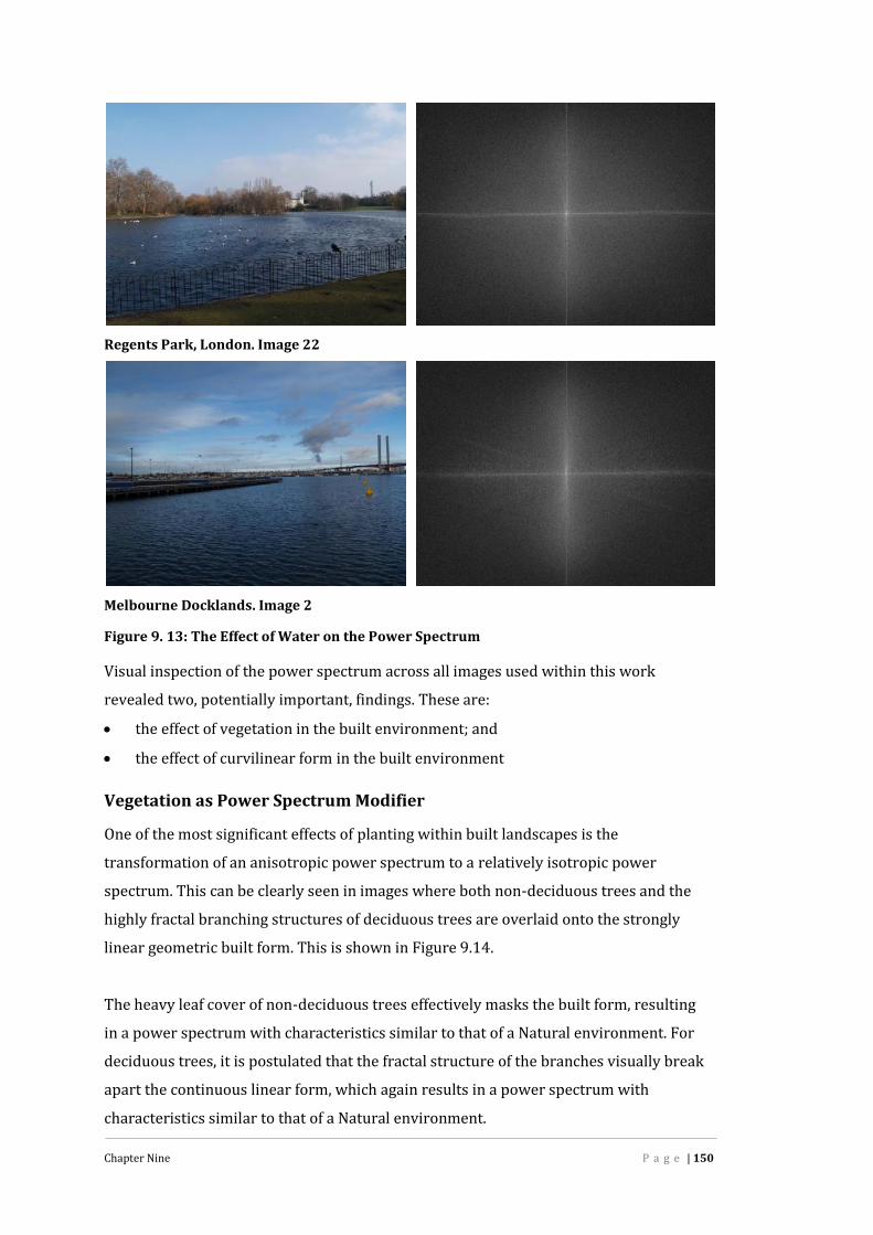
Chapter Nine P a g e | 150
Regents Park, London. Image 22
Melbourne Docklands. Image 2
Figure 9. 13: The Effect of Water on the Power SpectrumVisual inspection of the power spectrum across all images used within this workrevealed two, potentially important, findings. These are: the effect of vegetation in the built environment; and the effect of curvilinear form in the built environmentVegetation as Power Spectrum ModifierOne of the most significant effects of planting within built landscapes is thetransformation of an anisotropic power spectrum to a relatively isotropic powerspectrum. This can be clearly seen in images where both non-deciduous trees and thehighly fractal branching structures of deciduous trees are overlaid onto the stronglylinear geometric built form. This is shown in Figure 9.14.The heavy leaf cover of non-deciduous trees effectively masks the built form, resultingin a power spectrum with characteristics similar to that of a Natural environment. Fordeciduous trees, it is postulated that the fractal structure of the branches visually breakapart the continuous linear form, which again results in a power spectrum withcharacteristics similar to that of a Natural environment.

Chapter Nine P a g e | 151
Cambridge, UK. Image 18
Central Brisbane City, Image 26
London West One, Image 14
Figure 9. 14: The Effect of Vegetation on the Power SpectrumAlthough the comparison of the small number of images within this study cannot beseen as proof of this modifying effect, the underlying principles describing thegeneration of a power spectrum points towards its validity. The author considers thatthis is the first time the concept of using vegetation to ‘soften’ the urban built form hasbeen clearly and objectively demonstrated.

Chapter Nine P a g e | 152
Curvilinear Form as Power Spectrum ModifierFigure 9.15 shows the only image across all the landscapes studied that contains adistinct curvilinear built form. If this were a linear form, the power spectrum would beexpected to display high energy lines corresponding to the strong perspective lines thatsuch a form would create. However, the power spectrum is relatively isotropic.Therefore, it may be hypothesised that curvilinear Para-natural forms create anisotropic power spectrum similar to that of Natural environments, which provides a‘softer’ experiential aspect to the spatial form.
London West One, Image 7
Figure 9. 15: The Effect of Curvilinear Form on the Power Spectrum
This argument is supported by the images in Figure 9.16 of two relatively new buildingfacades within Brisbane CBD. Building 1 is an example of a building that exhibits manycurvilinear structures on its facade. Whereas Building 2 has a very linear geometricform. It can be seen that the three-dimensional pattern formed by the modular panelsof curvilinear lines of the facade of Building One generates a power spectrum that hascharacteristics more in common with those of Wild Nature, than the power spectrumproduced by the facade of Building Two. These findings point towards the conclusionthat with suitable detailed design, vegetation is not required as an ameliorating agentto reduce the high energy power spectrum lines produce by linear geometric forms.

Chapter Nine P a g e | 153
Building One
Building Two
Figure 9. 16: Building Facades, Central Brisbane City
Although further information from the power spectrum is difficult to obtain withoutimage analysis tools far more advanced than those accessibly to this research, it ispossible to determine the range of amplitudes of the component frequencies within thepower spectrum through a simple analysis technique within R97, known as a KernelDensity Estimation. This was undertaken as a form of data triangulation.Kernel Density EstimationKernel Density Estimation (KDE) is a graphical data representation technique similar tothat of a histogram. However, histograms do not produce a smooth curve, as theydepend on the width of the bins (the equal intervals into which the whole data range issub-divided) and the end points of the bins (where each of the bins starts and stops).This is shown graphically in Appendix E.
97 R is the statistical software used for all the analysis in this work

Chapter Nine P a g e | 154
Power Spectrum Median AmplitudeThe big advantage of the KDE method for representing data is that it removes thedependence on bin width and end points and produces a smooth curve. (Doug 2001).Appendix E shows the KDE plots for the images within each landscape that have thehighest, the median and the lowest fractal dimensions. Superimposed onto each of theplots is the power spectrum median amplitude (PSMA) for each of the images98. Figure9.17 shows two examples.
Regents Park, London Cranbourne Botanic Gardens
Figure 9. 17: Example Kernel Density Estimation PlotsThe KDE plots graph the number of frequency points within the power spectrum of aparticular image that have the same amplitude. Therefore, the plots shown above forRegents Park, London and Cranbourne Botanic Gardens, Victoria, represent the energyshift within in the landscape from the images which have the highest, the median andthe lowest fractal dimensions.It can be seen that for Regents Park, there is not much change in the energy distributionas the fractal dimension changes. However, for Cranbourne Botanic Gardens the energyshifts from higher numbers of low amplitude frequencies to lower numbers of higheramplitude frequencies. Although each landscape studied exhibits its own particularenergy shift pattern, it can be seen from the data in Appendix C - Section 2 that themeasured PSMAs vary between a limited range of values having a minimum of 38 and amaximum of 84 across the 21 landscapes studied. Figure 9.18 shows the overall medianvalue of the PSMA for all 21 landscapes ordered from lowest to highest and shown withthe Vegetation Rating.98 The median power spectrum amplitude for each image and the overall median powerspectrum amplitude for each landscape are documented in Appendix A.

Chapter Nine P a g e | 155
Figure 9. 18: Landscape vs Power Spectrum Median AmplitudeLike the median fractal dimension the distribution of the overall median values of thePSMA for each landscape studied displays a linear trend. This linear trend increases asthe landscape forms change from predominantly geometric built forms topredominantly vegetation. However, again Dundowran Beach is an interesting case asit is a landscape form close to Wild Nature, but has the lowest PSMA of all landscapesstudied.The statistical validity of this data (P < 0.22e-15) is supported by the ANOVA results inTable 9.1 below. This P value is extremely small and gives strong evidence to reject anyclaim that all landscapes will have the same PSMA. However, similar to the analysis forfractal dimensions, to ensure that the results of the ANOVA test are not due to chanceas a result of multiple comparison errors, a Tukey’s honest significance difference test,with a 95 per cent confidence interval, was applied to the data. The results of this testare documented in Appendix D, Section 2 and show that of the 210 uniquecomparisons, 157 were significantly different, or about 75 percent.Although there appears to be a strong link between the PSMA and landscape type(Figure 9.18), there does not seem to be a comparative link between the PSMA and thefractal dimension. This is demonstrated in Figure 9.19, which is based on the data fromall 1085 images included in this study. The R2 value of 0.3714 confirms that the linkbetween the two-dimensional PSMA and fractal dimension is weak, when consideredon an image by image basis for the landscapes studied.

Chapter Nine P a g e | 156
Table 9. 1: ANOVA Results for Power Spectrum Median Amplitude
Estimate Std. Error t value Pr(>|t|) SignificanceIntercept 2.547483 0.011177 227.921 < 2e-16 5LandscapeBCBG 74.3125 1.0054 73.915 < 2e-16 4CB -4.0937 1.4218 -2.879 0.004066 5CBC -19.4588 1.3415 -14.505 < 2e-16 5CBG -14.6319 1.2083 -12.109 < 2e-16 5CFL -11.16 1.2486 -8.938 < 2e-16 5CHR -16.5347 1.3818 -11.966 < 2e-16 1CTC -0.1258 1.2009 -0.105 0.916565 5DB -7.8317 1.2778 -6.129 1.24E-09 5GP -25.639 1.2926 -19.835 < 2e-16 1HBBGa 1.1042 1.5357 0.719 0.472309 1HBBGb -1.3125 1.3729 -0.956 0.3393 5HBE 4.7481 1.411 3.365 0.000792 5LEC -8.0194 1.2524 -6.403 2.27E-10 5LW -10.6809 1.2563 -8.502 < 2e-16 5MD -13.7038 1.1672 -11.741 < 2e-16 5RP -22.7336 1.3645 -16.66 < 2e-16 5RSP -5.4159 1.2524 -4.325 1.67E-05 5SBP -6.1146 1.1609 -5.267 1.68E-07 5StJP -6.8125 1.1985 -5.684 1.69E-08 1TCC -1.767 1.5751 -1.122 0.262179 5
SignificanceCodes
5 = 0 4 = 0.001 3 = 0.01 2 = 0.05 1 = 0.1
Residual standard error: 5.687 on 1069 degrees of freedomMultiple R-squared: 0.6198, Adjusted R-squared: 0.6126F-statistic: 87.12 on 20 and 1069 DFP < 2.20e-16
Figure 9. 19: Power Spectrum Median Amplitude vs. Fractal Dimension

Chapter Nine P a g e | 157
As discussed in Chapter 6, the fractal dimension is a measure derived from an analysisof the slope of the line-of-best-fit of the one-dimensional power spectrum of each rowand column within an image. The PSMA is a direct measure from within the two-dimensional power spectrum of each image, independent of frequency. Although bothmeasures are derived from the power spectrums, the results of the KDE analysisdiscussed above validates the proposition that the PSMA be considered a new indicatorof landscape form.If a digital image is considered as a textural pattern that represents the structuralcomplexity of a real world environment, then this outcome parallels the requirementsfor more information than just the fractal dimension when trying to quantifying thatcomplexity (Turner et al. 1998, 50). The requirement for more than one parameter todifferentiate between images is also supported by Pan et al in their work ondistinguishing between computer generated images and natural images using fractalgeometry (Pan et al. 2009).The data contained in Figure 9.18 confirms that like the fractal dimension, images fromwithin different landscapes can exhibit the same level of PSMA, whilst exhibitingdifferent fractal dimensions. Examples of this are shown in Figure 9.20.
South Bank Parklands, Image 34Vegetation Rating = 3
Fractal Dimension = 2.432PSMA = 60
London West One, Image 5Vegetation Rating = 2
Fractal Dimension = 2.393PSMA = 60
Figure 9. 20: Power Spectrum Median Amplitude vs LandscapeHowever, although the discussion above shows that both the fractal dimension and thePSMA by themselves cannot differentiate between all individual images from withindifferent landscapes, when used together, they show a much greater ability to do so.This is demonstrated in Figure 9.21 for the images shown in Figure 9.1. It can be seen

Chapter Nine P a g e | 158
that the combination of the fractal dimension and PSMA values allows easydifferentiates between these images.
Central Brisbane City, Image 4Vegetation Rating = 1
Fractal Dimension = 2.516PSMA = 67
Chermside Hills Reserve, Image 53Vegetation Rating = 5
Fractal Dimension = 2.516PSMA = 72
London West One, Image 71Vegetation Rating = 1
Fractal Dimension = 2.384PSMA = 64
Dundowran Beach, Image 50Vegetation Rating = 1
Fractal Dimension = 2.384PSMA = 43
Figure 9. 21: Power Spectrum Median Amplitude vs Fractal DimensionsFrom Chapter 6, we know that that the fractal dimension represents the level of self-similarity within an image. This is determined from the slope of the line of best fit of theone-dimensional power spectra for all rows and columns within an image. Whereas, thePSMA value of the two-dimensional power spectrum is a measure of the overall powerlevels within the image.Power Spectrum Median Amplitude and Landscape FormUnlike the fractal dimension, which is dependent on the relative amplitudes of thefrequencies within the power spectrum, the value of the PSMA is dependent on the

Chapter Nine P a g e | 159
absolute magnitudes of the component frequencies. This is demonstrated in Figure 9.22which shows the frequency amplitudes for a single row from images with a high, lowand a mid-range median PSMA.
London West One, Image 43, Median PSMA = 47
Hervey Bay Esplanade, Image 33, Median PSMA = 65
Hervey Bay Botanic Gardens B, Image 11, Median PSMA = 84
Figure 9. 22: One Dimensional PSMA LevelsFigure 9.22 indicates the number of frequency points in the one-dimensional powerspectrum for the specified rows within each image. It can be seen that for the imagewith the lowest median PSMA, the number of frequency points above the zero line is341. For the image with a mid level median PSMA rating the number of frequencypoints above the zero line is 628. For the image with the highest median PSMA ratingthe number of frequency points above the zero line is 1117. Although the analysis onthese rows is indicative only, it demonstrates that the higher the magnitude of the

Chapter Nine P a g e | 160
amplitudes of the component frequencies in the two-dimensional power spectrum, thehigher the median PSMA value.From the discussion in Chapter 6, it can be seen that the magnitude of the frequencycomponents in the power spectrum are dependent on the luminance values of adjacentpixels within the image―their contrast. Therefore, the higher contrast betweenadjacent pixels, the greater the amplitudes of the component power spectrumfrequencies. This high contrast also allows greater discernment of fine detail.This is demonstrated in Figure 9.23 which shows an image from Hervey Bay BotanicGardens―Part B and from Melbourne Docklands. It can be seen that the level of finedetail and pixel luminance values is much greater in image HBBGb11 than in imageMD26. This is reflected in the power spectrums, where image MD26 displays a markedreduction in the amplitudes of the higher frequencies. This is confirmed by the KernelDensity Estimation plots in Figure 9.24, which shows that the range of amplitudes ofthe frequencies in image MD26 are much lower than those in image HBBGb11.
Image HBBGb11, PSMA = 84, Fractal Dimension = 2.633
Image MD26, PSMA = 48, Fractal Dimension = 2.475
Figure 9. 23: Effects of Image Contrast on Fractal Dimension and PSMA

Chapter Nine P a g e | 161
Figure 9. 24: Effects of Image Structure on Frequency AmplitudeThese finding do not reflect the level of isotropy, which is based on the frequencydistribution in the power spectrum, but range of frequency amplitudes.Contribution to KnowledgeThe underlying structural geometry of a landscape has been shown to display a uniquepattern of energy distribution―a form of structural signature of a landscape. Thissignature can be characterised by three parameters: overall median Fractal dimension; overall PSMA and level of isotropy within the power spectrum.Although the power spectrum is not a new concept, its application to the analyses ofoverall landscape form has revealed significant structural differences between Naturaland Para-natural environments that have not been previously identified. The PSMA of alandscape is, as far as the author is aware, a completely new parameter for describingand interpreting environments. When combined with the level of isotropy and thefractal dimension, these three provide a new lens through which greater understandingof the underlying structural properties of a landscape can be gainedConclusionRuderman (1997) has proposed that “ The properties of our visual world greatlyinfluence the design of creatures’ visual systems”. This is supported by the field of

Chapter Nine P a g e | 162
psychophysics (Field 1987; Cormac and Stamenov 1996) and reflects the propositionby Bourassa, (previously discussed in Chapter 5), that aesthetics has a biological basis.Bourassa’s proposition is somewhat supported by Cooper et al (2010) who concludedthat there was a positive association between the rating of visual quality and the fractaldimension of urban street scenes. Similarly, the research by Berg (2007) supports thefindings by previous researchers (Kaplan and Kaplan 1989; Purcell et al. 2001) thatNatural environments with a certain level of fractal dimension or that containsignificant levels of vegetation are far more effective at reducing stress than Para-natural environments composed of mainly Euclidean geometric built forms.It is proposed here that the three parameters of fractal dimension, the PSMA and thelevel of isotropy within the power spectrum form part of an unarticulated ‘language’embedded within the underlying structural geometry of a landscape. It is clear from theresults of the analyses in this work that these three parameters relate directly to thestructural geometry of both Wild Nature and Designed Nature. It is also clear that thescale at which a landscape is experienced, where scale can be either physical ortemporal, can have a marked effect on these parameters.However, the primary goal of this research has been to increase our knowledge andunderstanding of how fractal geometry can be used as a referent for future landscapedesign forms and how it can support the articulation of an aesthetic for ecologicaldesign. In Chapter 5, it was seen that an aesthetic is considered to be composed of twomajor components: an aesthetic experience or response and an aesthetic property orquality. Putting aside the subjective vs. objective arguments with respect to these, it isclear that both the form and the content of a landscape design must possess propertiesthat initiate a positive aesthetic response in the users of that landscape. What is alsoclear is that Wild Nature has no teleological end point. Wild Nature is continuallychanging and evolving over time—it is, in effect, unfinished. Therefore, the forms andcontent of any ecological designs must also embody the concept of change. This isdiscussed in the final chapter ― Chapter 10.

Chapter Ten P a g e | 163
Chapter Ten
The Unfinished Landscape
IntroductionAs already discussed, Catherin Bull (1996, 27) has argued that the content of landscapedesign is “nature”. What has been shown here is that the content of landscape design isactually Nature, both Wild Nature and Designed Nature in their infinitely varieddynamic combinations that are constantly changing. Lawrence Halprin (Quoted byHowett 1987, 11) understands this when he says:...in ecology what is significant is not so much the understanding of whatexists at any given moment in time, but that existence is ephemeral and inconstant motion, constant change.The infinite patterns of Wild Nature were recently addressed in the landscapearchitecture electronic forum ‘LARCH’ by the American landscape architect EdwardFlaherty (2010). He suggested that our current approach to land and ecologicalplanning has its roots in the two-dimensional plans derived from the complex overlayprocess used within Geographic Information Systems. As an adjunct to this discussionhe asked:When Mandelbrot used computer power with Julia Sets in the late 1970s, theresulting Mandelbrot Set gave us infinitely evolving lines...have landscapearchitects addressed this Mandelbrot Set math as a basis for theory or design?In response to this, Richard Sutton (2010) from the University of New Englandsuggested that the feedback loops inherent in any design processes mirror therecursive processes of Wild-Nature or the Mandelbrot Set and that therefore, design isfractal by nature.Although Sutton’s conception of recursion is simplistic, there are some clear analogiesbetween the Mandelbrot Set, Natural environments and Para-natural environments. Asdiscussed in Chapter 3, the Mandelbrot set is the visualisation of the solutions to theequation: = + . Examples of this, originally shown as Figure 3.12, arereprinted here (Figure 10.1).

Chapter Ten P a g e | 164
Figure 10. 1: Figure 3.12 ReprintedThe black areas within the pattern visually represent where the solutions to theequation are stable and unchanging― the actual Mandelbrot Set. These areas can beseen as a metaphor for our primary Western design paradigm that rejects the constantevolution and dynamic change of Wild Nature and tries to create finishedproducts―like a work of art. However, our aesthetic of finishedness requires a high levelof maintenance to ensure that the final constructed designed is maintained against theinexorable changes driven by Wild Nature and social processes (Sutton and Anderson
2010) . This level of maintenance usually requires significant Para-natural processes,and hence secondary energy, to achieve. Therefore, natural processes ensure that afinished landscape is never actually realised and in reality is a true Sisyphean task. Incontrast, the patterns at the edge of the Mandelbrot Set are where the solutions to theequation are never stable. Here the forms are quasi self-similar and infinitely variedover all scales of observation. They are an echo of the infinite variation of an unfinishedWild Nature.

Chapter Ten P a g e | 165
However, change does not mean that a whole landscape needs to be in continuousmotion. Heraclitus, an ancient Greek philosopher who lived around 500 BCE believedthat the underlying law of Nature is that nothing can be identified with any particularsubstance, but rather with an ongoing process governed by a law of change (Graham2011, 89). His most recognised quote is that “... you could not step twice into the sameriver”. What this actually means, is that something must be continually changing forother things to exist and remain the same. If water did not flow in a river, then the riverwould not exist. Similarly, if plant communities did not grow, change, mature and diethey would remain static and eventually die out. This is recognised by Nigel Dunnett(2004, 98) when he says:Any acceptance of an ecologically-informed approach to planting must fullyembrace the concept of change. The common perception that plantcommunities in the wild are relatively static, with little alteration in thecomposition or appearance from year to year, is of course a misconception:change is fundamental to the processes that operate within semi-naturalplant communities. Indeed it could be said that every ecological principle thata designer or manager needs to be aware of is related in some way to thisdynamic nature of plant communities.If we are to achieve true sustainability the unfinishedness of Wild Nature must berecognised and incorporated as a conscious design parameter (Nohl 2001; Harker et al.1999). Such designs could be developed from the underlying fractal dimension, PSMAand Level of Isotropy of their regional context, with specific user requirements derivedfrom the local level. They must also recognise that social patterns of use change andevolve just as Wild Nature changes and evolves. Thus sustainable designs, in a humancontext, must also become responsive and capable of adapting to these changes(Bentley et al. 1985). Therefore, such designs must also be legible, not only fornavigation and way finding, but also in terms of their ecological sustainability.Towards an Ecological AestheticThe practice of landscape design operates at the interface between the old and the new.Our current Western design paradigm of finishedness, as discussed, must be replacedwith a new paradigm that also recognises the dynamic order and complexity of WildNature, a dynamic system embodied by the infinite and ever changing patternsdescribed by fractal geometry. The understanding that the patterns Wild Nature areself-similar is fundamental. This by itself can be used to develop new design forms.
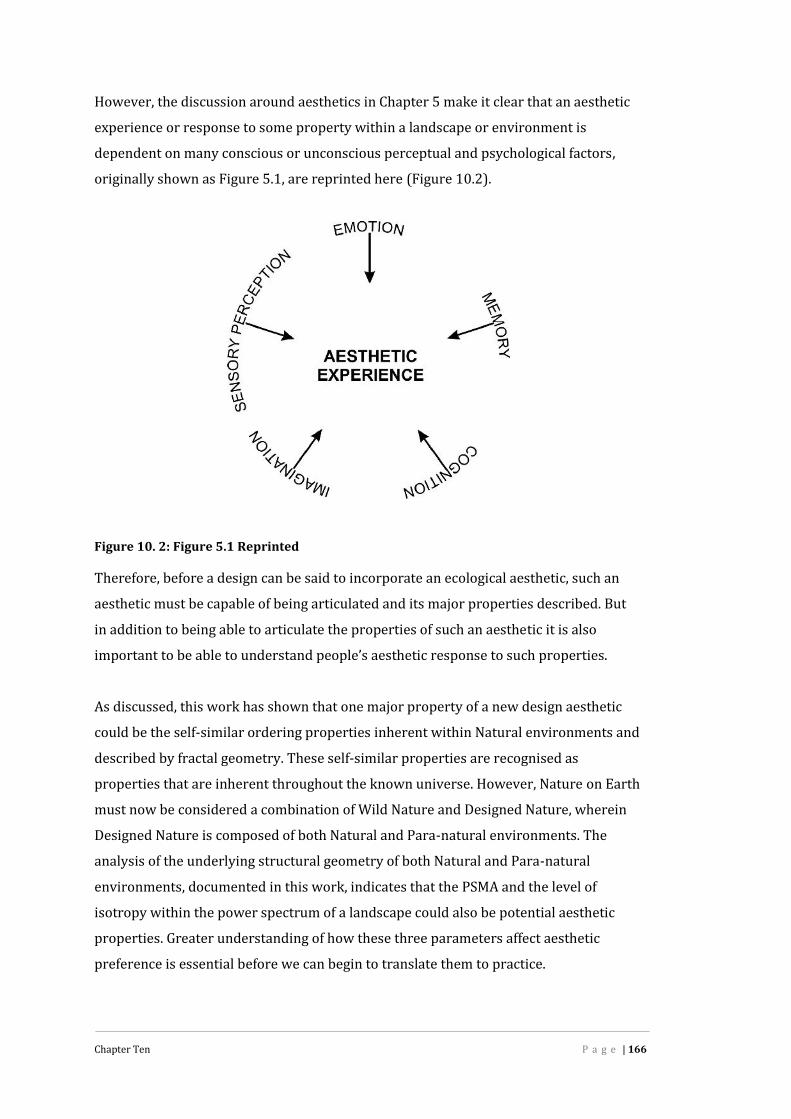
Chapter Ten P a g e | 166
However, the discussion around aesthetics in Chapter 5 make it clear that an aestheticexperience or response to some property within a landscape or environment isdependent on many conscious or unconscious perceptual and psychological factors,originally shown as Figure 5.1, are reprinted here (Figure 10.2).
Figure 10. 2: Figure 5.1 ReprintedTherefore, before a design can be said to incorporate an ecological aesthetic, such anaesthetic must be capable of being articulated and its major properties described. Butin addition to being able to articulate the properties of such an aesthetic it is alsoimportant to be able to understand people’s aesthetic response to such properties.As discussed, this work has shown that one major property of a new design aestheticcould be the self-similar ordering properties inherent within Natural environments anddescribed by fractal geometry. These self-similar properties are recognised asproperties that are inherent throughout the known universe. However, Nature on Earthmust now be considered a combination of Wild Nature and Designed Nature, whereinDesigned Nature is composed of both Natural and Para-natural environments. Theanalysis of the underlying structural geometry of both Natural and Para-naturalenvironments, documented in this work, indicates that the PSMA and the level ofisotropy within the power spectrum of a landscape could also be potential aestheticproperties. Greater understanding of how these three parameters affect aestheticpreference is essential before we can begin to translate them to practice.

Chapter Ten P a g e | 167
It has already been shown that people have a preference for the self-similar fractalpatterns of Wild Nature. Therefore, it is clear that we need to begin to consciouslydesign and allow these patterns into our everyday environments at all scales, fromregions down to private gardens. However, the relationship between preference andfractal patterns may not be linear. Too little or too much fractal complexity may resultis a drop in preference. This non-linearity may also apply to both the PSMA and thelevel of isotropy within the power spectrum.It is clear that landscape design based solely on principles derived from visual art doesnot allow for any rational or objective decision as to how a design will affect aestheticpreference. Neither does landscape design based solely on ecological principles allowthis determination. However, this new work has articulated three parameters derivedfrom the underlying structural geometry of both Natural and Designed environmentsthat moves us a step closer to being able to make these rational and objectiveassessments. Similarly, the results presented here suggest that these three parametersmay be able to quantify such concepts as spatial complexity and form (Kaplan 1982;Kaplan and Kaplan 1989; Kaplan et al. 1998).Clearly, there is yet more work to do. This must include: studies to examine the effect of light quality on the fractal dimension, powerspectrum median amplitude and level of isotropy on a digital image. studies to examine the relationship between landscape preference and the fractaldimension99, the PSMA and the level of isotropy within a landscape; refinement of the model used for fractal analysis of digital images; further analysis of the landscape power spectrum with more powerful tools toelicit deeper information on the structural geometry of landscapes; and the development of a method to quantify the level of isotropy within a digitalimage and hence an overall landscape.This work articulates a completely new way to understand the spatial structure andpatterns embedded within a landscape. However, it is clear that these findings must betaken as preliminary and that further work will bring clarity. Nevertheless, afoundation has been built based on greater understanding of the ways fractal geometryand the underlying structural geometry of a landscape might be used to further99 The work by Knill et al (1990) and Spehar et al (2003) is supported by the recent work byCooper et a (2010) and suggests that the Fractal dimension may affect landscape preference.

Chapter Ten P a g e | 168
ecologically sustainable design. Similarly, this work contains the kernel of ideasrequired for future articulation of an ecological aesthetic.

Appendix A P a g e | 169
Appendix A: Camera and Analysis Software
Digital Cameras and Image QualityThe camera chosen for this study was the Olympus E300 digital single lens reflexcamera, fitted with the standard 14-45mm lens. This choice was governed by the manypositive professional reviews of the cameras quality and the cost. All photographs forthis study were taken with the following camera settings:Exposure mode―in ‘P’ or Program mode the camera sets the optimum aperture valueand shutter speed automatically according to the subject brightness.Focus― the Olympus 300E uses three focus control frames to achieve camera focus.These are illustrated in Figure A.1.
Figure A. 1: Olympus E300 Focus Control FramesUsing these frames, the camera has three focus modes: S-AF―single auto focus C-AF―continuous auto focus MF―Manual focusFor this study, the camera was set to ‘S-AF+MF’ mode, which uses the single auto-focusmode and allows for manual focus adjustment if required.ISO―The ISO function adjusts the cameras sensitivity to light. This was set toAutomatic.Metering―The metering in the camera measures the subject brightness. The Olympus300E has three metering modes: Digital ESP― the camera meters and calculates the light levels of light leveldifferences in the centre and other areas of the image.

Appendix A P a g e | 170
Centre weighted averaging―the camera provides the average metering betweenthe subject and the background lighting. Spot metering―the camera meters a very small area around the centre of thesubject.As the subject of each image is the whole image, rather than any particular section of animage, the Digital ESP metering mode was selected.Record Mode― As well as raw image data and TIFF100 formats, the E300 camera hasthree standard JPEG101 record modes: Super High Quality, High Quality and StandardQuality. Each of these three modes can be used with different image compressionlevels. These are shown in Table A.1 with the pixel count for each mode.Table A. 1: Olympus E300 Record Modes
Pixels Compression Level
None 1:2.7 1:4 1:8
3264 x 2448 TIFF SHQ HQ HQ
3200 x 2400
SQ
2560 x 2400
1600 x 1200
1280 x 960
1024 x 768
640 x 480
As can be seen in Table A.1, the record mode allows a choice to be made between thenumber of pixels and the compression level within an image. What needs to taken intoconsideration is that when an image with a low pixel count is enlarged to show itsstructure, it will display a much greater mosaic effect, or pixilation, than an image witha larger pixel count. This is clarified in Table A.2, which shows a section of the image inFigure A.2 magnified to 1600% of the original size for a sample of the pixel count andcompression ratios available..
100 Tagged Image File Format101 Joint Photographic Experts Group

Appendix A P a g e | 171
Figure A. 2: Test Image
Table A. 2: Record Mode vs Image Quality
Record Mode Zoom Record Mode Zoom
Pixels: 3264 x 2448
Compression: 1:2.7
File Size: 5.10MB
# of Images102 = 155
Pixels: 1280 x 960
Compression: 1:2.7
File Size: 779 KB
# of Images: 1055
Pixels: 3264 x 2448
Compression: 1:4
File Size: 3.87 MB
# of Images: 222
Pixels: 1024 x 768
Compression: 1:2.7
File Size: 500 KB
# of Images: 1161
Pixels: 3200 x 2400
Compression: 1:2.7
File Size: 5.69 MB
# of Images: 161
Pixels: 640 x 480
Compression: 1:2.7
File Size: 204 KB
# of Images: 3912
102 The ‘# of images’ is the total number of images capable of being recorded on a 1 GB FlashCard for that particular pixel/compression combination. This parameter was a factor in the finaldecision as to which record mode to use.

Appendix A P a g e | 172
Record Mode Zoom Record Mode Zoom
Pixels: 2560 x 1920
Compression: 1:2.7
File Size: 3.66 MB
# of Image: 241
Pixels: 1600 x 1200
Compression: 1:2.7
File Size: 1.26 MB
# of Images: 688
It can be seen that the lower the pixel count and the higher the compression the lowerthe image quality, which results in greater the pixilation and the loss of clarity anddetail within the image.Choosing the recode mode was a trade off between image quality, file size and thenumber of images capable of being recorded in the E300 at any one time. Table A.1shows that the compression levels for the HQ mode is either 1:4 or 1:8, whereas thecompression levels for the SHQ and SQ modes can go as low as 1:2.7. Table A.2indicates that the file size for the SHQ mode is considerably greater than for the HQ orSQ modes.

Appendix A P a g e | 173
Fractal Analysis Code for R
mean.and.std<-function(x = rnorm(10)){av<- mean(x)sd <-sqrt(var(x))c(mean=av, SD=sd)
}
loadimg<-function(imgname='Le_lorrain.jpg'){x<-read.jpeg(imgname)if (length(dim(x))!= 2)
x<-rgb2grey(x)}
subsample<-function(x,ssr,ssc){#takes the first pixel of first row, and then every ssr'th collumn#takes a subsample of rows, taking every ssc'th row
lenx1<-dim(x)[1]lenx2<-dim(x)[2]leny1<-floor(lenx1/ssr)leny2<-floor(lenx2/ssc)y<-mat.or.vec(leny1,leny2)dim(y)<-c(leny1,leny2)for (i in 1:leny1){
for (j in 1:leny2){#y[i,j]<-x[ (i-1)*ssr + 1, (j-1)*ssc + 1]#Take the mean value of the region of size ssr*sscy[i,j]<-mean(x[((i-1)*ssr+1):(i*ssr), ((j-1)*ssc + 1):
(j*ssc)])}
}z<-imagematrix(y)
}
sym_extend<-function(x){len1<-dim(x)[1]len2<-dim(x)[2]sx<-mat.or.vec(2*len1,2*len2)sx[1:len1,1:len2]<-x[1:len1,1:len2]sx[(len1+1):(2*len1),1:len2]<-x[len1:1,1:len2]sx[1:len1,(len2+1):(2*len2)]<-x[1:len1,len2:1]sx[(len1+1):(2*len1),(len2+1):(2*len2)]<-x[len1:1,len2:1]imagematrix(sx)
}
fracfit2D<-function(x,f=1,weight=1,sym=0){#x is the image#f is a flag for printing graphs, printed if f==1#w is the flag for weighting the least squares solution by the# inverse of the number of points in each frequency band# if weight = 2, fit to an average in each band# if sym=1, symmetrically extend image#load required packagelibrary(boot)library(rimage)
if (sym==1){# symmetrically extend the signal to avoid difficulties with
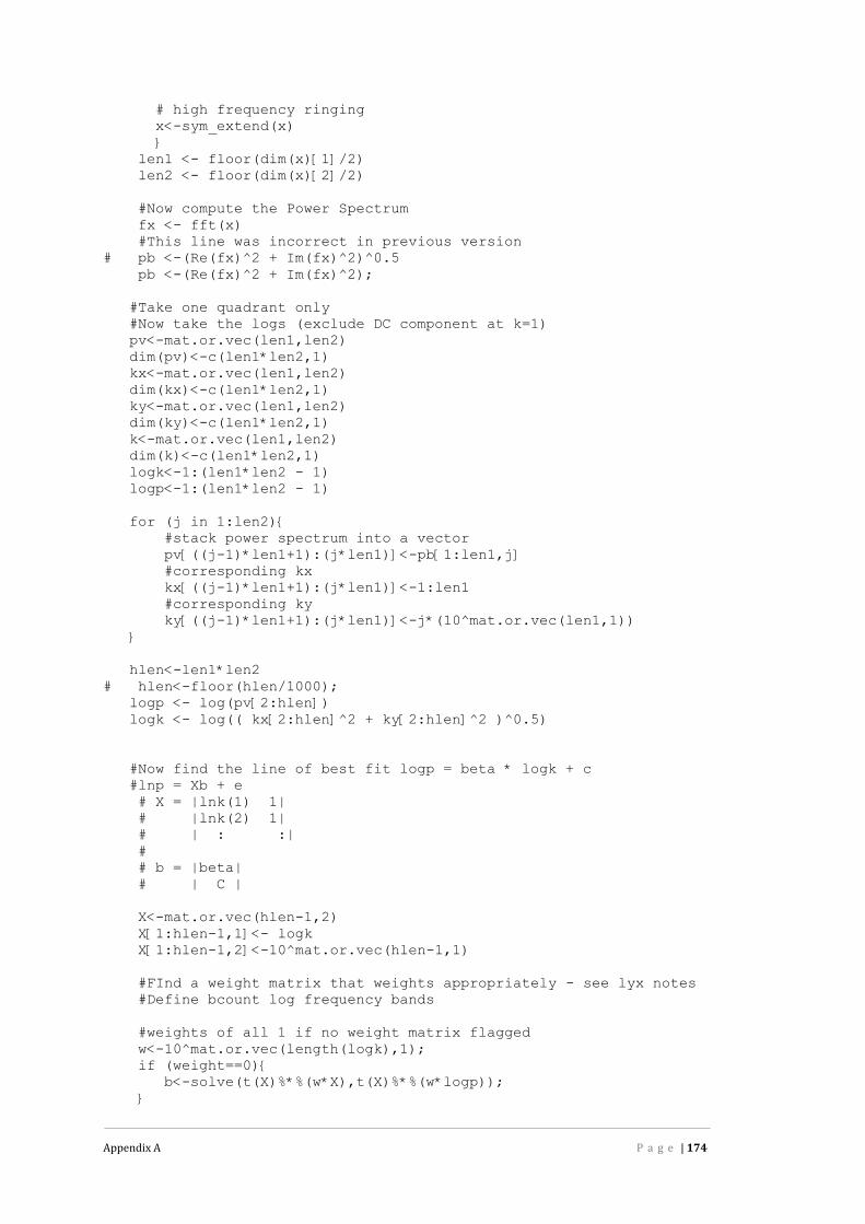
Appendix A P a g e | 174
# high frequency ringingx<-sym_extend(x)}
len1 <- floor(dim(x)[1]/2)len2 <- floor(dim(x)[2]/2)
#Now compute the Power Spectrumfx <- fft(x)#This line was incorrect in previous version
# pb <-(Re(fx)^2 + Im(fx)^2)^0.5pb <-(Re(fx)^2 + Im(fx)^2);
#Take one quadrant only#Now take the logs (exclude DC component at k=1)pv<-mat.or.vec(len1,len2)dim(pv)<-c(len1*len2,1)kx<-mat.or.vec(len1,len2)dim(kx)<-c(len1*len2,1)ky<-mat.or.vec(len1,len2)dim(ky)<-c(len1*len2,1)k<-mat.or.vec(len1,len2)dim(k)<-c(len1*len2,1)logk<-1:(len1*len2 - 1)logp<-1:(len1*len2 - 1)
for (j in 1:len2){#stack power spectrum into a vectorpv[((j-1)*len1+1):(j*len1)]<-pb[1:len1,j]#corresponding kxkx[((j-1)*len1+1):(j*len1)]<-1:len1#corresponding kyky[((j-1)*len1+1):(j*len1)]<-j*(10^mat.or.vec(len1,1))
}
hlen<-len1*len2# hlen<-floor(hlen/1000);
logp <- log(pv[2:hlen])logk <- log(( kx[2:hlen]^2 + ky[2:hlen]^2 )^0.5)
#Now find the line of best fit logp = beta * logk + c#lnp = Xb + e# X = |lnk(1) 1|# |lnk(2) 1|# | : :|## b = |beta|# | C |
X<-mat.or.vec(hlen-1,2)X[1:hlen-1,1]<- logkX[1:hlen-1,2]<-10^mat.or.vec(hlen-1,1)
#FInd a weight matrix that weights appropriately - see lyx notes#Define bcount log frequency bands
#weights of all 1 if no weight matrix flaggedw<-10^mat.or.vec(length(logk),1);if (weight==0){
b<-solve(t(X)%*%(w*X),t(X)%*%(w*logp));}

Appendix A P a g e | 175
if (weight==1){bcount<-25bands<-1:bcountbands<-(max(logk)-min(logk))/bcount * bands +
min(logk)*10^mat.or.vec(bcount,1)bands<-c(min(logk),bands)
#To find counts in each band, use the histogram functionh<-hist(logk,bands,plot=FALSE)cumcount<-h$counts#Convert to cumulative countsfor (i in 2:bcount){
cumcount[i]<-cumcount[i]+ cumcount[i-1]}#prepend a zero countcumcount<-c(0,cumcount)
#order the log frequenciesord<-order(logk)
#construct the weight matrix#This will be just 7 1/7's 16 1/16ths etc where counts are
7,16,...
for (i in 2:length(h$counts)){w[ (cumcount[i-1]+1):(cumcount[i])]<- w[ (cumcount[i-
1]+1):(cumcount[i])]/h$count[i-1]}#wm<-diag(w)
b<-solve(t(X)%*%(w*X),t(X)%*%(w*logp))
}#the wm matrix becomes too large if we try and do normal matrix
multiplication#Do array multiplication instead, as wm is a diagonal matrix.#b[1] contains the slope beta#b[2] contains the intercept C
if (weight==2){bcount<-25bands<-1:bcountbands<-(max(logk)-min(logk))/bcount * bands +
min(logk)*10^mat.or.vec(bcount,1)bands<-c(min(logk),bands)
#To find counts in each band, use the histogram functionh<-hist(logk,bands,plot=FALSE)cumcount<-h$counts#Convert to cumulative countsfor (i in 2:bcount){
cumcount[i]<-cumcount[i]+ cumcount[i-1]}#prepend a zero countcumcount<-c(0,cumcount)
#order the log frequencies#ord<-order(logk)
#construct new logk and logp vectors by taking the middle logkfrom each

Appendix A P a g e | 176
#band and the average logp from each band
newlogp<-mat.or.vec(bcount,1);for (i in 1:bcount){
newlogp[i]<-mean(logp[cumcount[i]+1]:logp[cumcount[i+1]]);}
newlogk<-mat.or.vec(bcount,1);for (i in 1:bcount){
#newlogk[i]<-logk[cumcount[i]+floor(h$counts[i]/2)];newlogk<-h$mids;
}
#New X vectorX<-mat.or.vec(bcount,2)X[1:bcount,1]<- newlogkX[1:bcount,2]<-10^mat.or.vec(bcount,1)
b<-solve(t(X)%*%X,t(X)%*%newlogp)
}
if (f==1){#graph the power spectrumif (weight ==2){
plot(newlogk,newlogp,pch="*");}else{
plot(logk,logp,pch=".");}
}
if (f==1){#add regression line to plotlinex<-c(min(logk),max(logk))liney<-b[2] + b[1]*linexlines(linex,liney)
}
#compute the fractal dimension D = 4+beta/2D <- 4 + b[1]/2
#Need to relook at this so that takes into account the weightingintroduce
#above for addresing the different numbers of obs at each logfrequency
resid <- logp - (logk*b[1]+b[2])sdr <- sd(resid)#create a matrix g for computing the correlationg<-mat.or.vec(length(logp),2)dim(g)<-c(length(logp),2)g[1:length(logp),1]<-logk[1:length(logp)]g[1:length(logp),2]<-logp[1:length(logp)]R2<-(corr(g))^2NR<-sdr^2/sd(logp)^2
c(D=D, R2=R2)
#c(length=len, SD=sd)
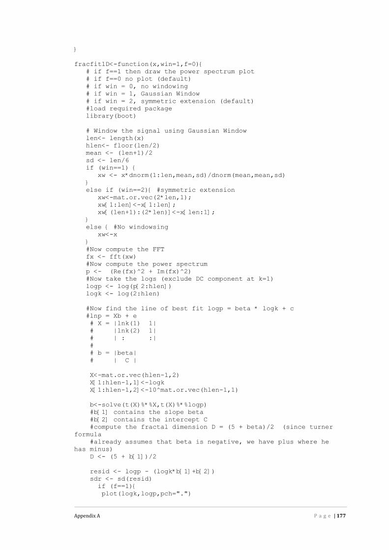
Appendix A P a g e | 177
}
fracfit1D<-function(x,win=1,f=0){# if f==1 then draw the power spectrum plot# if f==0 no plot (default)# if win = 0, no windowing# if win = 1, Gaussian Window# if win = 2, symmetric extension (default)#load required packagelibrary(boot)
# Window the signal using Gaussian Windowlen<- length(x)hlen<- floor(len/2)mean <- (len+1)/2sd <- len/6if (win==1) {
xw <- x*dnorm(1:len,mean,sd)/dnorm(mean,mean,sd)}else if (win==2){ #symmetric extension
xw<-mat.or.vec(2*len,1);xw[1:len]<-x[1:len];xw[(len+1):(2*len)]<-x[len:1];
}else { #No windowsing
xw<-x}#Now compute the FFTfx <- fft(xw)#Now compute the power spectrump <- (Re(fx)^2 + Im(fx)^2)#Now take the logs (exclude DC component at k=1)logp <- log(p[2:hlen])logk <- log(2:hlen)
#Now find the line of best fit logp = beta * logk + c#lnp = Xb + e# X = |lnk(1) 1|# |lnk(2) 1|# | : :|## b = |beta|# | C |
X<-mat.or.vec(hlen-1,2)X[1:hlen-1,1]<-logkX[1:hlen-1,2]<-10^mat.or.vec(hlen-1,1)
b<-solve(t(X)%*%X,t(X)%*%logp)#b[1] contains the slope beta#b[2] contains the intercept C#compute the fractal dimension D = (5 + beta)/2 (since turner
formula#already assumes that beta is negative, we have plus where he
has minus)D <- (5 + b[1])/2
resid <- logp - (logk*b[1]+b[2])sdr <- sd(resid)
if (f==1){plot(logk,logp,pch=".")

Appendix A P a g e | 178
#add regression line to plotlinex<-c(min(logk),max(logk))liney<-b[2] + b[1]*linexlines(linex,liney)
}
#create a matrix g for computing the correlationg<-mat.or.vec(length(logp),2)dim(g)<-c(length(logp),2)g[1:length(logp),1]<-logk[1:length(logp)]g[1:length(logp),2]<-logp[1:length(logp)]R2<-(corr(g))^2
#standard deviation of residualsSR <- sd(resid)
c(D=D, R2=R2, SR=SR)
#c(length=len, SD=sd)}
vsa<-function(x, win=1){#defaults to Gaussian WindowNrows<-dim(x)[1]Ncols<-dim(x)[2]a<-mat.or.vec(Nrows,3);for (i in 1:Nrows) {
a[i,]<-fracfit1D(x[i,],win,0)}
b<-mat.or.vec(Ncols,3);for (j in 1:Ncols) {
b[j,]<-fracfit1D(x[,j],win,0)}
#Overall#mean 1d fractal dimensionD1bar <- mean(c(a[,1],b[,1]));#std 1d fractal dimension#D1std <- sd(c(a[,1],b[,1]));#mean R2#R2bar <-mean(c(a[,2],b[,2]));#R2std <- sd(c(a[,2],b[,2]));
#mean SR#SRbar <- mean(c(a[,3],b[,3]));#SRstd <- sd(c(a[,3],b[,3]));
#XD1barX <- mean(c(b[,1]));#std 1d fractal dimensionD1stdX <- sd(c(b[,1]));#mean R2R2barX <-mean(c(b[,2]));R2stdX <- sd(c(b[,2]));
#mean SR#SRbarX <- mean(c(b[,3]));#SRstdX <- sd(c(b[,3]));
#YD1barY <- mean(c(a[,1]));

Appendix A P a g e | 179
#std 1d fractal dimensionD1stdY <- sd(c(a[,1]));#mean R2R2barY <-mean(c(a[,2]));R2stdY <- sd(c(a[,2]));
#mean SR#SRbarY <- mean(c(a[,3]));#SRstdY <- sd(c(a[,3]));
D2 <- D1bar + 1;c(DX=D1barX, DXstd=D1stdX, R2X=R2barX, R2Xstd=R2stdX, DY=D1barY,
DYstd=D1stdY, R2Y=R2barY, R2Ystd=R2stdY, D2=D2);}
batchVsa<-function(directory){imlist<-dir(directory);#out<-mat.or.vec(length(imlist),2);outVsa<-mat.or.vec(length(imlist),9);outName<-mat.or.vec(length(imlist),1);i<-1;for (name in imlist){
outName[i]<-name;x<-loadimg(paste(directory,"/",name,sep=""));
# out[i,]<-fracfit2D(x);outVsa[i,]<-vsa(x);i<-i+1;
}ov<-data.frame(Image=outName,DX=outVsa[,1],DXstd=outVsa[,2],R2X=outVsa[,3],R2Xstd=outVsa[,4],DY=outVsa[,5],DYstd=outVsa[,6],R2Y=outVsa[,7],R2Ystd=outVsa[,8],D2=outVsa[,9]);c(ov=ov);}
batchFF2D<-function(directory){imlist<-dir(directory);out<-mat.or.vec(length(imlist),2);#outVsa<-mat.or.vec(length(imlist),9);outName<-mat.or.vec(length(imlist),1);i<-1;for (name in imlist){
outName[i]<-name;x<-loadimg(paste(directory,"/",name,sep=""));out[i,]<-fracfit2D(x);
# outVsa[i,]<-vsa(x);i<-i+1;
}ff2d<-data.frame(Image=outName,D=out[,1],R2=out[,2]);c(ff2d=ff2d);}

Appendix B P a g e | 180
Appendix B: Vegetation Rating
Notes:1. V Rating = Vegetation RatingTable B. 1: Vegetation Rating forBrisbane Botanic Gardens
Table B. 2: Vegetation Rating for Brisbane CityBotanic Gardens
Image V RatingBBG12 4BBG2 4BBG21 4BBG24 4BBG25 4BBG3 4BBG30 4BBG5 4BBG6 4BBG1 5BBG10 5BBG11 5BBG14 5BBG15 5BBG16 5BBG17 5BBG18 5BBG19 5BBG20 5BBG22 5BBG23 5BBG26 5BBG27 5BBG28 5BBG29 5BBG31 5BBG32 5BBG4 5BBG7 5BBG8 5BBG9 5Median 5
Image V RatingBCBG12 4BCBG15 4BCBG23 4BCBG24 4BCBG27 4BCBG28 4BCBG3 4BCBG30 4BCBG1 5BCBG10 5BCBG11 5BCBG13 5BCBG14 5BCBG16 5BCBG17 5BCBG18 5BCBG19 5BCBG2 5BCBG20 5BCBG21 5BCBG22 5BCBG25 5BCBG26 5BCBG29 5BCBG31 5BCBG32 5BCBG4 5BCBG5 5BCBG6 5BCBG7 5BCBG8 5BCBG9 5Median 5.0

Appendix B P a g e | 181
Table B. 3: Vegetation Ratingfor Cambridge, UK
Table B. 4: Vegetation Rating for CentralBrisbane City
Image V RatingCB1 1CB10 1CB12 1CB14 1CB15 1CB16 1CB17 1CB19 1CB20 1CB23 1CB24 1CB26 1CB27 1CB29 1CB30 1CB31 1CB32 1CB35 1CB36 1CB37 1CB38 1CB39 1CB4 1CB40 1CB6 1CB7 1CB8 1CB11 2CB13 2CB21 2CB28 2CB41 2CB9 2CB22 3CB25 3CB5 3CB18 4CB2 4CB3 4CB43 4CB42 5Median 1
Image V Rating Image V RatingCBC10 1 CBC18 3CBC20 1 CBC21 3CBC37 1 CBC27 3CBC39 1 CBC29 3CBC41 1 CBC34 3CBC49 1 CBC38 3CBC53 1 CBC42 3CBC55 1 CBC44 3CBC67 1 CBC46 3CBC68 1 CBC48 3CBC7 1 CBC51 3CBC73 1 CBC52 3CBC8 1 CBC56 3CBC1 2 CBC57 3CBC11 2 CBC60 3CBC12 2 CBC61 3CBC15 2 CBC69 3CBC19 2 CBC70 3CBC2 2 CBC71 3CBC22 2 CBC13 4CBC24 2 CBC23 4CBC25 2 CBC26 4CBC28 2 CBC31 4CBC3 2 CBC35 4CBC30 2 CBC59 4CBC32 2CBC33 2 Median 2CBC36 2CBC4 2CBC40 2CBC43 2CBC45 2CBC47 2CBC5 2CBC50 2CBC54 2CBC58 2CBC6 2CBC62 2CBC63 2CBC65 2CBC66 2CBC72 2CBC9 2CBC14 3CBC16 3CBC17 3

Appendix B P a g e | 182
Table B. 5: Vegetation Rating for ChermsideHills Reserve, Brisbane
Table B. 6: Vegetation Rating for ChildersFarm Land, Qld
Image V Rating Image V RatingCHR8 4 CHR30 5CHR73 4 CHR23 5CHR6 4 CHR51 5CHR70 4 CHR38 5CHR17 5 CHR19 5CHR32 5 CHR36 5CHR29 5 CHR52 5CHR71 5 CHR28 5CHR3 5 CHR75 5CHR66 5 CHR27 5CHR61 5 CHR54 5CHR48 5 CHR13 5CHR41 5 CHR56 5CHR35 5 CHR63 5CHR31 5 CHR15 5CHR49 5 CHR34 5CHR64 5 CHR53 5CHR33 5 CHR65 5CHR72 5 CHR43 5CHR62 5 CHR24 5CHR60 5 CHR21 5CHR10 5 CHR69 5CHR47 5 CHR4 5CHR14 5 CHR46 5CHR26 5 CHR55 5CHR20 5 CHR12 5CHR44 5 CHR11 5CHR67 5 CHR76 5CHR74 5CHR68 5 Median 5CHR39 5CHR57 5CHR1 5CHR2 5CHR50 5CHR58 5CHR25 5CHR22 5CHR42 5CHR18 5CHR7 5CHR45 5CHR9 5CHR37 5CHR77 5CHR16 5CHR40 5
Image V RatingCFL35 2CFL31 2CFL36 2CFL29 2CFL33 2CFL28 3CFL30 3CFL32 3CFL25 3CFL27 3CFL11 4CFL7 4CFL8 4CFL9 4CFL20 4CFL34 4CFL10 4CFL18 4CFL22 4CFL19 4CFL17 4CFL26 4CFL21 4CFL24 4CFL6 4CFL12 4CFL4 4CFL5 4CFL3 4CFL14 4CFL23 4CFL15 4CFL13 4CFL16 4CFL1 4CFL2 4Median 4

Appendix B P a g e | 183
Table B. 7: Vegetation Rating for ChildersTown Centre, Qld
Table B. 8: Vegetation Rating for CranbourneBotanic Gardens, Vic
Image V Rating Image V RatingCTC48 1 CTC43 4CTC15 1 CTC28 4CTC13 1 CTC19 4CTC36 1 CTC11 4CTC40 2 CTC27 4CTC16 2 CTC52 4CTC50 2CTC39 2 Median 3CTC9 2CTC12 2CTC47 2CTC14 2CTC31 2CTC49 3CTC38 3CTC24 3CTC33 3CTC41 3CTC46 3CTC17 3CTC18 3CTC45 3CTC1 3CTC26 3CTC22 3CTC21 3CTC23 3CTC51 3CTC10 3CTC20 3CTC34 3CTC25 3CTC7 3CTC8 3CTC35 3CTC37 3CTC42 3CTC3 4CTC5 4CTC32 4CTC44 4CTC4 4CTC6 4CTC2 4CTC29 4CTC30 4
Image V Rating Image V RatingCBG33 1 CBG43 4CBG31 2 CBG42 4CBG5 2 CBG53 4CBG6 2 CBG22 4CBG29 2 CBG16 4CBG77 2 CBG74 4CBG30 2 CBG48 4CBG1 2 CBG70 4CBG67 2 CBG55 4CBG23 2 CBG71 4CBG75 2 CBG10 5CBG54 2 CBG39 5CBG49 3CBG17 3 Median 3CBG27 3CBG20 3CBG32 3CBG50 3CBG14 3CBG26 3CBG21 3CBG25 3CBG62 3CBG64 3CBG45 3CBG58 3CBG59 3CBG60 3CBG3 3CBG8 3CBG66 3CBG52 3CBG44 3CBG18 3CBG11 3CBG4 3CBG13 3CBG61 4CBG15 4CBG19 4CBG57 4CBG73 4CBG56 4CBG72 4CBG68 4CBG2 4
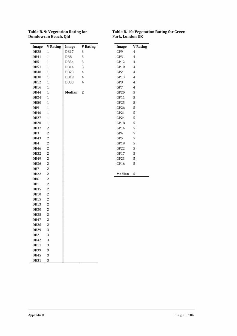
Appendix B P a g e | 184
Table B. 9: Vegetation Rating forDundowran Beach, Qld
Table B. 10: Vegetation Rating for GreenPark, London UK
Image V Rating Image V RatingDB28 1 DB17 3DB41 1 DB8 3DB5 1 DB34 3DB51 1 DB14 3DB48 1 DB23 4DB38 1 DB19 4DB12 1 DB33 4DB16 1DB44 1 Median 2DB24 1DB50 1DB9 1DB40 1DB27 1DB20 1DB37 2DB3 2DB43 2DB4 2DB46 2DB32 2DB49 2DB36 2DB7 2DB22 2DB6 2DB1 2DB35 2DB10 2DB15 2DB13 2DB30 2DB25 2DB47 2DB26 2DB29 3DB2 3DB42 3DB11 3DB39 3DB45 3DB31 3
Image V RatingGP9 4GP3 4GP12 4GP10 4GP2 4GP13 4GP8 4GP7 4GP20 5GP11 5GP25 5GP26 5GP21 5GP24 5GP18 5GP14 5GP4 5GP5 5GP19 5GP22 5GP17 5GP23 5GP16 5Median 5

Appendix B P a g e | 185
Table B. 11: Vegetation Rating for HerveyBay Botanic Gardens, Part A, Qld
Table B. 12: Vegetation Rating for HerveyBay Botanic Gardens, Part B, Qld
Image V RatingHBBGa35 4HBBGa20 4HBBGa8 4HBBGa22 4HBBGa28 4HBBGa10 4HBBGa32 4HBBGa4 4HBBGa3 4HBBGa5 4HBBGa9 4HBBGa33 4HBBGa12 4HBBGa2 4HBBGa7 4HBBGa13 5HBBGa16 5HBBGa29 5HBBGa30 5HBBGa18 5HBBGa17 5HBBGa11 5HBBGa36 5HBBGa21 5HBBGa23 5HBBGa34 5HBBGa37 5HBBGa24 5HBBGa26 5HBBGa19 5HBBGa1 5HBBGa14 5HBBGa6 5HBBGa15 5HBBGa25 5HBBGa31 5HBBGa27 5Median 4
Image V RatingHBBGb25 4HBBGb22 4HBBGb11 5HBBGb8 5HBBGb12 5HBBGb4 5HBBGb32 5HBBGb10 5HBBGb19 5HBBGb6 5HBBGb15 5HBBGb7 5HBBGb13 5HBBGb2 5HBBGb14 5HBBGb24 5HBBGb21 5HBBGb20 5HBBGb9 5HBBGb3 5HBBGb16 5HBBGb5 5HBBGb23 5HBBGb28 5HBBGb31 5HBBGb26 5HBBGb1 5HBBGb17 5HBBGb33 5HBBGb18 5HBBGb30 5HBBGb27 5HBBGb29 5Median 5
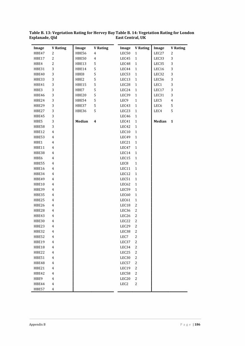
Appendix B P a g e | 186
Table B. 13: Vegetation Rating for Hervey BayEsplanade, Qld
Table B. 14: Vegetation Rating for LondonEast Central, UK
Image V Rating Image V RatingHBE47 2 HBE56 4HBE17 2 HBE50 4HBE4 2 HBE13 5HBE31 3 HBE14 5HBE40 3 HBE8 5HBE33 3 HBE2 5HBE41 3 HBE15 5HBE3 3 HBE7 5HBE46 3 HBE20 5HBE24 3 HBE54 5HBE29 3 HBE37 5HBE27 3 HBE36 5HBE45 3HBE5 3 Median 4HBE58 3HBE12 4HBE53 4HBE1 4HBE11 4HBE38 4HBE6 4HBE55 4HBE16 4HBE34 4HBE49 4HBE10 4HBE39 4HBE35 4HBE25 4HBE26 4HBE28 4HBE43 4HBE30 4HBE23 4HBE32 4HBE52 4HBE19 4HBE18 4HBE22 4HBE51 4HBE48 4HBE21 4HBE42 4HBE9 4HBE44 4HBE57 4
Image V Rating Image V RatingLEC50 1 LEC27 2LEC45 1 LEC33 3LEC48 1 LEC35 3LEC44 1 LEC16 3LEC53 1 LEC32 3LEC13 1 LEC56 3LEC28 1 LEC1 3LEC24 1 LEC17 3LEC39 1 LEC31 3LEC9 1 LEC5 4LEC43 1 LEC6 5LEC23 1 LEC4 5LEC46 1LEC41 1 Median 1LEC42 1LEC10 1LEC49 1LEC21 1LEC47 1LEC14 1LEC15 1LEC8 1LEC11 1LEC12 1LEC51 1LEC62 1LEC59 1LEC60 1LEC61 1LEC18 2LEC36 2LEC26 2LEC22 2LEC29 2LEC38 2LEC7 2LEC37 2LEC34 2LEC25 2LEC30 2LEC57 2LEC19 2LEC58 2LEC20 2LEC2 2

Appendix B P a g e | 187
Table B. 15: Vegetation Rating for LondonWest One, UK
Table B. 16: Vegetation Rating for MelbourneDocklands, Vic
Image V Rating Image V RatingLW91 1 LW75 1LW96 1 LW42 1LW90 1 LW66 1LW36 1 LW52 1LW95 1 LW74 1LW67 1 LW58 1LW25 1 LW31 1LW83 1 LW37 1LW24 1 LW2 1LW38 1 LW43 1LW17 1 LW10 2LW49 1 LW70 2LW47 1 LW15 2LW19 1 LW40 2LW23 1 LW93 2LW35 1 LW4 2LW68 1 LW55 2LW57 1 LW59 2LW77 1 LW54 2LW63 1 LW45 2LW28 1 LW48 2LW61 1 LW71 2LW20 1 LW76 2LW18 1 LW8 2LW3 1 LW5 2LW16 1 LW60 2LW50 1 LW82 2LW44 1 LW72 2LW41 1 LW73 2LW56 1 LW92 3LW26 1 LW14 3LW27 1 LW6 3LW21 1 LW7 3LW86 1 LW81 3LW29 1 LW12 3LW62 1 LW78 4LW65 1 LW9 4LW46 1 LW13 4LW53 1 LW39 4LW22 1 LW80 4LW1 1 LW85 5LW69 1 LW84 5LW30 1 LW94 5LW64 1 LW79 5LW51 1 LW11 5LW34 1Median 1
Image V RatingMD34 1MD7 1MD38 1MD39 1MD6 1MD4 1MD19 1MD24 1MD18 1MD5 1MD15 1MD22 1MD11 1MD16 1MD20 1MD21 1MD28 1MD1 1MD29 1MD8 1MD3 1MD26 1MD23 1MD2 1MD27 1MD10 1MD33 1MD35 2MD12 2MD36 2MD31 2MD17 2MD14 2MD37 2MD9 2MD30 2MD32 3MD13 3Median 1

Appendix B P a g e | 188
Table B. 17: Vegetation Rating for RegentsPark, London UK
Table B. 18: Vegetation Rating for RomaStreet Parklands, Brisbane
Image V Rating Image V RatingRP22 2 RP17 5RP56 3 RP37 5RP10 3 RP46 5RP9 3 RP36 5RP25 3 RP47 5RP26 3 RP63 5RP15 3 RP57 5RP18 3 RP64 5RP11 3 RP38 5RP14 3 RP41 5RP44 4RP61 4 Median 4RP3 4RP16 4RP2 4RP7 4RP29 4RP5 4RP6 4RP23 4RP28 4RP27 4RP55 4RP1 4RP43 4RP51 4RP8 4RP30 4RP34 4RP60 4RP4 4RP62 4RP48 4RP35 4RP31 4RP54 4RP24 4RP53 4RP49 4RP58 4RP42 4RP52 4RP33 4RP40 4RP39 4RP59 5RP45 5
Image V Rating Image V RatingRSP96 1 RSP81 4RSP50 1 RSP45 4RSP10 2 RSP53 4RSP40 2 RSP20 4RSP26 2 RSP63 4RSP88 2 RSP5 4RSP38 3 RSP84 4RSP39 3 RSP42 4RSP17 3 RSP91 4RSP1 3 RSP6 4RSP67 3 RSP21 4RSP2 3 RSP33 4RSP34 3 RSP64 4RSP27 3 RSP46 4RSP24 3 RSP15 4RSP93 3 RSP61 4RSP29 3 RSP86 4RSP3 3 RSP78 5RSP19 3 RSP73 5RSP43 3 RSP12 5RSP95 3 RSP60 5RSP4 3 RSP76 5RSP89 3 RSP23 5RSP28 3 RSP90 5RSP32 4 RSP68 5RSP41 4 RSP13 5RSP79 4 RSP25 5RSP8 4 RSP7 5RSP31 4 RSP47 5RSP69 4 RSP54 5RSP75 4 RSP72 5RSP56 4 RSP52 5RSP92 4 RSP57 5RSP22 4 RSP55 5RSP65 4 RSP14 5RSP30 4 RSP51 5RSP59 4 RSP83 5RSP80 4 RSP66 5RSP87 4 RSP44 5RSP82 4 RSP77 5RSP49 4 RSP62 5RSP85 4 RSP18 5RSP37 4 RSP16 5RSP74 4 RSP71 5RSP36 4 RSP11 5RSP48 4 RSP58 5RSP9 4 RSP70 5RSP94 4RSP35 4 Median 4
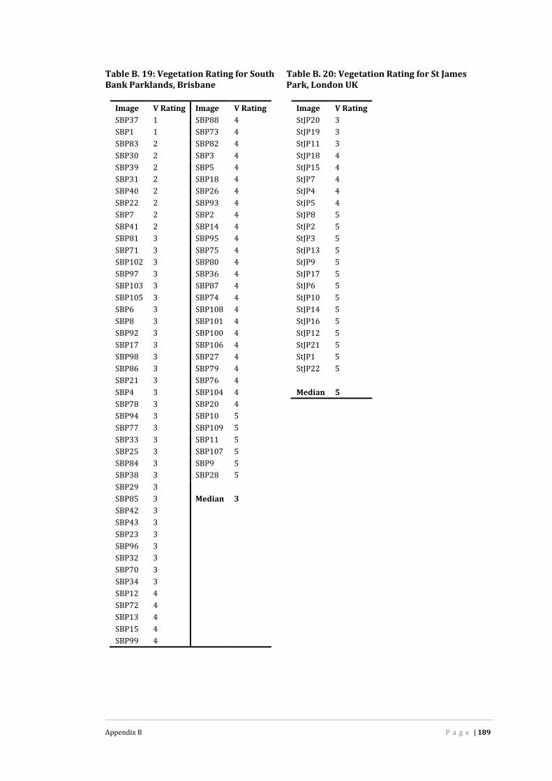
Appendix B P a g e | 189
Table B. 19: Vegetation Rating for SouthBank Parklands, Brisbane
Table B. 20: Vegetation Rating for St JamesPark, London UK
Image V Rating Image V RatingSBP37 1 SBP88 4SBP1 1 SBP73 4SBP83 2 SBP82 4SBP30 2 SBP3 4SBP39 2 SBP5 4SBP31 2 SBP18 4SBP40 2 SBP26 4SBP22 2 SBP93 4SBP7 2 SBP2 4SBP41 2 SBP14 4SBP81 3 SBP95 4SBP71 3 SBP75 4SBP102 3 SBP80 4SBP97 3 SBP36 4SBP103 3 SBP87 4SBP105 3 SBP74 4SBP6 3 SBP108 4SBP8 3 SBP101 4SBP92 3 SBP100 4SBP17 3 SBP106 4SBP98 3 SBP27 4SBP86 3 SBP79 4SBP21 3 SBP76 4SBP4 3 SBP104 4SBP78 3 SBP20 4SBP94 3 SBP10 5SBP77 3 SBP109 5SBP33 3 SBP11 5SBP25 3 SBP107 5SBP84 3 SBP9 5SBP38 3 SBP28 5SBP29 3SBP85 3 Median 3SBP42 3SBP43 3SBP23 3SBP96 3SBP32 3SBP70 3SBP34 3SBP12 4SBP72 4SBP13 4SBP15 4SBP99 4
Image V RatingStJP20 3StJP19 3StJP11 3StJP18 4StJP15 4StJP7 4StJP4 4StJP5 4StJP8 5StJP2 5StJP3 5StJP13 5StJP9 5StJP17 5StJP6 5StJP10 5StJP14 5StJP16 5StJP12 5StJP21 5StJP1 5StJP22 5Median 5

Appendix B P a g e | 190
Table B. 21: Vegetation Rating for Toowoomba City Centre, Qld
Image V Rating Image V RatingTCC7 1 TCC38 3TCC36 1 TCC12 4TCC8 1 TCC32 4TCC44 1 TCC21 4TCC16 1 TCC27 4TCC29 1 TCC5 4TCC42 1TCC35 1 Median 2TCC41 1TCC10 1TCC2 1TCC9 1TCC47 1TCC51 1TCC18 1TCC3 1TCC33 1TCC45 1TCC34 1TCC1 1TCC40 1TCC13 1TCC39 1TCC19 1TCC49 2TCC22 2TCC11 2TCC50 2TCC37 2TCC48 2TCC23 2TCC25 2TCC20 2TCC30 2TCC26 2TCC14 2TCC46 2TCC28 2TCC24 2TCC31 3TCC6 3TCC43 3TCC15 3TCC4 3TCC17 3
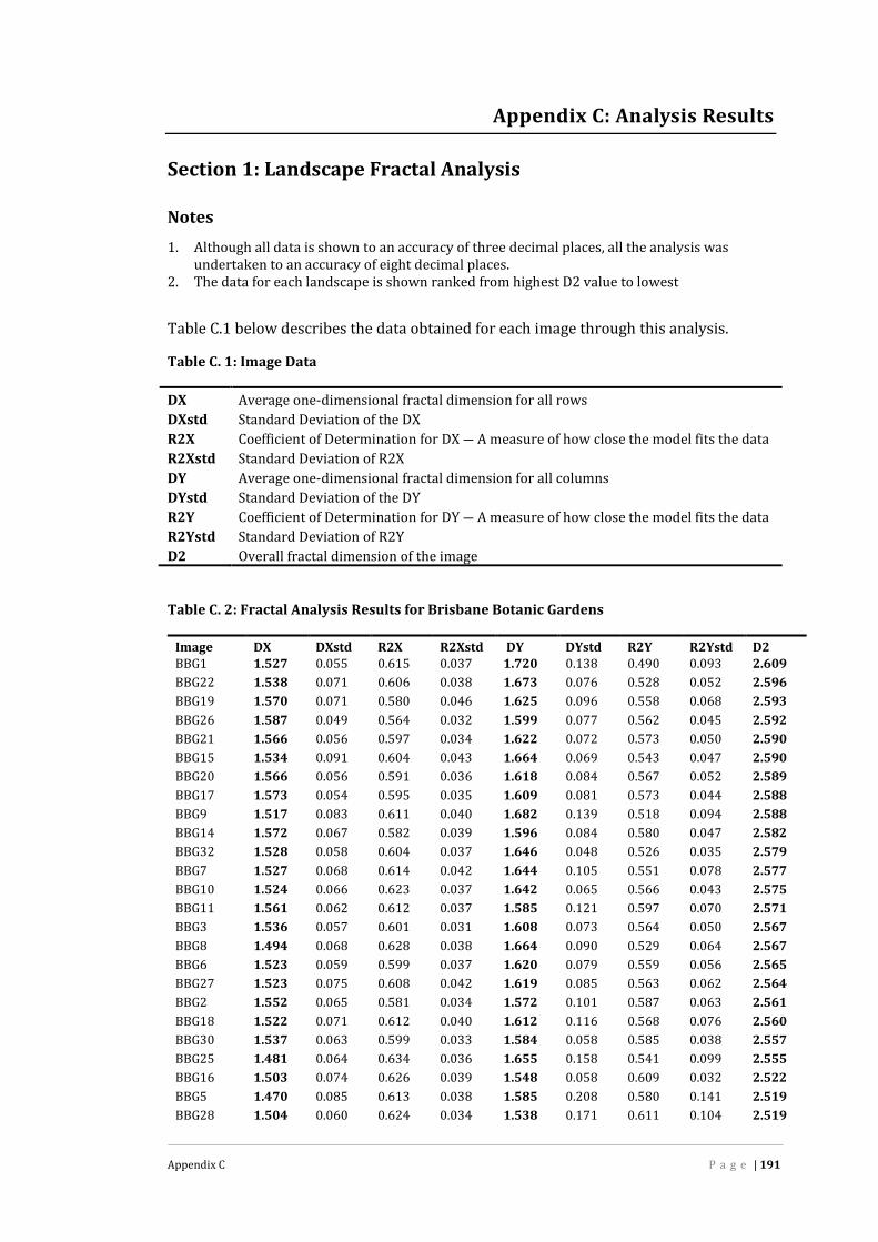
Appendix C P a g e | 191
Appendix C: Analysis Results
Section 1: Landscape Fractal Analysis
Notes1. Although all data is shown to an accuracy of three decimal places, all the analysis wasundertaken to an accuracy of eight decimal places.2. The data for each landscape is shown ranked from highest D2 value to lowestTable C.1 below describes the data obtained for each image through this analysis.Table C. 1: Image Data
DX Average one-dimensional fractal dimension for all rowsDXstd Standard Deviation of the DXR2X Coefficient of Determination for DX ― A measure of how close the model fits the dataR2Xstd Standard Deviation of R2XDY Average one-dimensional fractal dimension for all columnsDYstd Standard Deviation of the DYR2Y Coefficient of Determination for DY ― A measure of how close the model fits the dataR2Ystd Standard Deviation of R2YD2 Overall fractal dimension of the imageTable C. 2: Fractal Analysis Results for Brisbane Botanic Gardens
Image DX DXstd R2X R2Xstd DY DYstd R2Y R2Ystd D2BBG1 1.527 0.055 0.615 0.037 1.720 0.138 0.490 0.093 2.609BBG22 1.538 0.071 0.606 0.038 1.673 0.076 0.528 0.052 2.596BBG19 1.570 0.071 0.580 0.046 1.625 0.096 0.558 0.068 2.593BBG26 1.587 0.049 0.564 0.032 1.599 0.077 0.562 0.045 2.592BBG21 1.566 0.056 0.597 0.034 1.622 0.072 0.573 0.050 2.590BBG15 1.534 0.091 0.604 0.043 1.664 0.069 0.543 0.047 2.590BBG20 1.566 0.056 0.591 0.036 1.618 0.084 0.567 0.052 2.589BBG17 1.573 0.054 0.595 0.035 1.609 0.081 0.573 0.044 2.588BBG9 1.517 0.083 0.611 0.040 1.682 0.139 0.518 0.094 2.588BBG14 1.572 0.067 0.582 0.039 1.596 0.084 0.580 0.047 2.582BBG32 1.528 0.058 0.604 0.037 1.646 0.048 0.526 0.035 2.579BBG7 1.527 0.068 0.614 0.042 1.644 0.105 0.551 0.078 2.577BBG10 1.524 0.066 0.623 0.037 1.642 0.065 0.566 0.043 2.575BBG11 1.561 0.062 0.612 0.037 1.585 0.121 0.597 0.070 2.571BBG3 1.536 0.057 0.601 0.031 1.608 0.073 0.564 0.050 2.567BBG8 1.494 0.068 0.628 0.038 1.664 0.090 0.529 0.064 2.567BBG6 1.523 0.059 0.599 0.037 1.620 0.079 0.559 0.056 2.565BBG27 1.523 0.075 0.608 0.042 1.619 0.085 0.563 0.062 2.564BBG2 1.552 0.065 0.581 0.034 1.572 0.101 0.587 0.063 2.561BBG18 1.522 0.071 0.612 0.040 1.612 0.116 0.568 0.076 2.560BBG30 1.537 0.063 0.599 0.033 1.584 0.058 0.585 0.038 2.557BBG25 1.481 0.064 0.634 0.036 1.655 0.158 0.541 0.099 2.555BBG16 1.503 0.074 0.626 0.039 1.548 0.058 0.609 0.032 2.522BBG5 1.470 0.085 0.613 0.038 1.585 0.208 0.580 0.141 2.519BBG28 1.504 0.060 0.624 0.034 1.538 0.171 0.611 0.104 2.519

Appendix C P a g e | 192
BBG24 1.472 0.056 0.627 0.031 1.575 0.102 0.573 0.061 2.516BBG12 1.468 0.060 0.636 0.032 1.575 0.095 0.605 0.052 2.514BBG23 1.430 0.070 0.652 0.043 1.574 0.098 0.560 0.062 2.491BBG31 1.474 0.083 0.631 0.045 1.512 0.113 0.620 0.066 2.490BBG4 1.378 0.080 0.666 0.032 1.476 0.079 0.622 0.054 2.420BBG29 1.398 0.073 0.669 0.038 1.435 0.101 0.664 0.059 2.414
Median 1.524 0.066 0.612 0.037 1.609 0.090 0.567 0.059 2.567StdDev 0.048
Table C. 3: Fractal Analysis Results for Brisbane City Botanic Gardens
Image DX DXstd R2X R2Xstd DY DYstd R2Y R2Ystd D2BCBG13 1.556 0.054 0.589 0.037 1.638 0.093 0.547 0.058 2.591BCBG17 1.574 0.066 0.587 0.042 1.601 0.085 0.578 0.044 2.585BCBG6 1.568 0.059 0.591 0.035 1.595 0.079 0.589 0.052 2.580BCBG20 1.511 0.059 0.616 0.037 1.640 0.154 0.553 0.108 2.566BCBG1 1.479 0.076 0.653 0.040 1.663 0.099 0.533 0.071 2.558BCBG9 1.465 0.074 0.637 0.041 1.670 0.131 0.524 0.084 2.553BCBG7 1.547 0.058 0.591 0.036 1.553 0.120 0.605 0.083 2.550BCBG30 1.517 0.057 0.601 0.035 1.584 0.095 0.587 0.068 2.546BCBG2 1.480 0.069 0.659 0.035 1.618 0.111 0.564 0.075 2.539BCBG21 1.484 0.061 0.628 0.036 1.609 0.158 0.562 0.110 2.538BCBG3 1.458 0.067 0.645 0.038 1.633 0.158 0.535 0.110 2.533BCBG19 1.492 0.080 0.628 0.048 1.575 0.077 0.598 0.046 2.528BCBG29 1.484 0.060 0.628 0.033 1.581 0.109 0.582 0.076 2.526BCBG5 1.462 0.052 0.644 0.032 1.603 0.172 0.569 0.120 2.522BCBG23 1.483 0.078 0.636 0.035 1.565 0.091 0.611 0.058 2.518BCBG31 1.489 0.065 0.634 0.039 1.547 0.101 0.612 0.056 2.514BCBG16 1.413 0.047 0.663 0.026 1.643 0.133 0.528 0.090 2.511BCBG8 1.411 0.061 0.652 0.028 1.627 0.104 0.549 0.062 2.503BCBG28 1.435 0.054 0.650 0.032 1.579 0.102 0.583 0.060 2.497BCBG12 1.459 0.062 0.625 0.029 1.541 0.156 0.599 0.077 2.495BCBG11 1.434 0.077 0.639 0.042 1.575 0.112 0.568 0.056 2.494BCBG15 1.452 0.074 0.636 0.038 1.548 0.113 0.601 0.067 2.493BCBG24 1.419 0.072 0.656 0.036 1.568 0.116 0.600 0.059 2.483BCBG14 1.432 0.066 0.655 0.039 1.497 0.089 0.625 0.050 2.460BCBG4 1.381 0.089 0.671 0.038 1.565 0.103 0.579 0.055 2.460BCBG10 1.403 0.066 0.652 0.033 1.518 0.112 0.607 0.049 2.452BCBG27 1.427 0.059 0.655 0.031 1.478 0.093 0.606 0.050 2.449BCBG26 1.416 0.066 0.651 0.039 1.467 0.081 0.637 0.051 2.437BCBG32 1.266 0.087 0.724 0.036 1.583 0.168 0.578 0.117 2.402BCBG22 1.420 0.073 0.650 0.037 1.341 0.129 0.695 0.051 2.386BCBG25 1.248 0.075 0.703 0.030 1.478 0.151 0.610 0.070 2.346BCBG18 1.275 0.123 0.722 0.046 1.349 0.073 0.690 0.051 2.307
Median 1.459 0.066 0.644 0.036 1.577 0.110 0.585 0.061 2.513StdDev 0.067

Appendix C P a g e | 193
Table C. 4: Fractal Analysis Results for Cambridge, UK
Image DX DXstd R2X R2Xstd DY DYstd R2Y R2Ystd D2CB43 1.565 0.075 0.602 0.065 1.767 0.149 0.496 0.098 2.652CB25 1.588 0.101 0.584 0.082 1.667 0.080 0.523 0.057 2.622CB18 1.590 0.063 0.582 0.034 1.635 0.075 0.572 0.053 2.609CB42 1.625 0.065 0.550 0.050 1.503 0.115 0.642 0.062 2.573CB9 1.553 0.091 0.608 0.065 1.568 0.113 0.608 0.080 2.559CB2 1.515 0.089 0.622 0.055 1.575 0.112 0.602 0.066 2.540CB11 1.495 0.128 0.652 0.075 1.564 0.081 0.598 0.059 2.524CB6 1.596 0.134 0.616 0.084 1.423 0.069 0.689 0.039 2.522CB21 1.483 0.065 0.651 0.044 1.573 0.260 0.602 0.168 2.522CB3 1.543 0.092 0.621 0.051 1.489 0.090 0.652 0.047 2.520CB22 1.468 0.069 0.665 0.042 1.585 0.219 0.602 0.137 2.518CB4 1.497 0.102 0.665 0.055 1.496 0.104 0.642 0.071 2.497CB14 1.523 0.228 0.641 0.149 1.444 0.122 0.691 0.056 2.489CB16 1.503 0.150 0.667 0.082 1.462 0.100 0.686 0.053 2.485CB5 1.464 0.099 0.631 0.056 1.504 0.086 0.628 0.058 2.481CB19 1.398 0.066 0.676 0.041 1.580 0.320 0.583 0.221 2.476CB20 1.498 0.101 0.635 0.051 1.442 0.066 0.669 0.029 2.474CB31 1.503 0.181 0.645 0.105 1.417 0.109 0.686 0.055 2.466CB29 1.334 0.069 0.691 0.038 1.637 0.327 0.543 0.217 2.464CB15 1.486 0.097 0.674 0.057 1.425 0.146 0.692 0.075 2.460CB17 1.456 0.075 0.676 0.049 1.444 0.161 0.660 0.082 2.451CB8 1.463 0.112 0.656 0.063 1.434 0.049 0.667 0.029 2.451CB13 1.447 0.073 0.651 0.042 1.450 0.072 0.668 0.058 2.448CB27 1.399 0.085 0.667 0.047 1.502 0.166 0.638 0.096 2.443CB1 1.428 0.080 0.683 0.042 1.463 0.070 0.661 0.034 2.443CB37 1.342 0.083 0.685 0.040 1.547 0.243 0.607 0.147 2.430CB28 1.401 0.082 0.663 0.046 1.461 0.098 0.672 0.055 2.427CB23 1.343 0.097 0.732 0.036 1.528 0.337 0.606 0.229 2.422CB41 1.403 0.077 0.672 0.046 1.447 0.077 0.665 0.049 2.422CB30 1.410 0.129 0.679 0.063 1.432 0.106 0.663 0.052 2.419CB7 1.398 0.100 0.673 0.056 1.444 0.073 0.672 0.043 2.418CB10 1.424 0.093 0.689 0.049 1.407 0.056 0.687 0.030 2.417CB36 1.386 0.080 0.684 0.047 1.451 0.110 0.664 0.048 2.414CB40 1.395 0.090 0.678 0.043 1.438 0.129 0.656 0.060 2.414CB24 1.368 0.077 0.705 0.039 1.462 0.139 0.675 0.090 2.408CB32 1.358 0.062 0.702 0.038 1.463 0.092 0.688 0.040 2.403CB26 1.384 0.084 0.678 0.039 1.419 0.133 0.673 0.057 2.399CB38 1.325 0.096 0.695 0.048 1.435 0.147 0.671 0.077 2.372CB12 1.361 0.087 0.703 0.033 1.385 0.058 0.680 0.051 2.371CB35 1.351 0.102 0.701 0.046 1.391 0.098 0.684 0.046 2.368CB39 1.311 0.088 0.709 0.040 1.420 0.089 0.667 0.043 2.358
Median 1.447 0.089 0.667 0.048 1.462 0.106 0.663 0.057 2.451StdDev 0.070

Appendix C P a g e | 194
Table C. 5: Fractal Analysis Results for Central Brisbane City
Image DX DXstd R2X R2Xstd DY DYstd R2Y R2Ystd D2CBC4 1.539 0.088 0.621 0.051 1.465 0.159 0.656 0.081 2.516CBC36 1.522 0.115 0.612 0.078 1.505 0.118 0.622 0.063 2.515CBC26 1.477 0.062 0.642 0.038 1.559 0.138 0.603 0.079 2.512CBC35 1.457 0.076 0.643 0.038 1.576 0.089 0.592 0.056 2.508CBC16 1.460 0.072 0.630 0.056 1.572 0.161 0.597 0.097 2.508CBC6 1.430 0.095 0.644 0.042 1.580 0.178 0.567 0.101 2.494CBC69 1.445 0.095 0.637 0.050 1.531 0.078 0.599 0.052 2.482CBC18 1.437 0.079 0.649 0.042 1.526 0.140 0.624 0.083 2.475CBC38 1.474 0.118 0.622 0.060 1.470 0.078 0.648 0.048 2.472CBC23 1.445 0.078 0.640 0.041 1.507 0.108 0.621 0.059 2.472CBC25 1.450 0.086 0.626 0.050 1.499 0.095 0.624 0.055 2.471CBC21 1.462 0.096 0.639 0.047 1.477 0.153 0.643 0.084 2.468CBC12 1.426 0.081 0.644 0.048 1.520 0.156 0.622 0.099 2.466CBC5 1.396 0.090 0.667 0.041 1.551 0.172 0.614 0.095 2.462CBC54 1.406 0.092 0.652 0.038 1.534 0.118 0.607 0.052 2.461CBC1 1.446 0.100 0.640 0.054 1.476 0.171 0.624 0.092 2.459CBC8 1.422 0.124 0.682 0.063 1.507 0.102 0.645 0.048 2.458CBC37 1.481 0.190 0.620 0.104 1.421 0.148 0.678 0.081 2.455CBC15 1.388 0.122 0.690 0.062 1.532 0.113 0.613 0.072 2.450CBC46 1.416 0.067 0.644 0.037 1.492 0.169 0.618 0.092 2.449CBC19 1.399 0.070 0.665 0.033 1.514 0.130 0.637 0.063 2.448CBC56 1.392 0.083 0.679 0.038 1.516 0.183 0.619 0.097 2.445CBC42 1.484 0.105 0.611 0.065 1.383 0.100 0.671 0.044 2.440CBC43 1.429 0.099 0.644 0.064 1.453 0.175 0.644 0.112 2.439CBC17 1.456 0.102 0.665 0.054 1.416 0.089 0.674 0.044 2.439CBC50 1.422 0.086 0.650 0.044 1.458 0.110 0.654 0.058 2.438CBC51 1.417 0.080 0.655 0.045 1.461 0.084 0.647 0.048 2.436CBC52 1.398 0.071 0.664 0.046 1.485 0.169 0.637 0.099 2.435CBC61 1.419 0.052 0.641 0.034 1.445 0.075 0.642 0.037 2.431CBC72 1.388 0.078 0.676 0.044 1.485 0.178 0.655 0.109 2.429CBC9 1.384 0.085 0.679 0.048 1.487 0.145 0.582 0.092 2.428CBC48 1.380 0.125 0.672 0.056 1.487 0.123 0.637 0.055 2.426CBC45 1.333 0.106 0.702 0.047 1.549 0.150 0.589 0.104 2.426CBC22 1.410 0.102 0.653 0.047 1.440 0.184 0.654 0.104 2.423CBC62 1.375 0.112 0.651 0.056 1.487 0.202 0.617 0.109 2.423CBC2 1.400 0.152 0.664 0.067 1.448 0.127 0.657 0.072 2.421CBC20 1.401 0.079 0.649 0.046 1.435 0.149 0.662 0.087 2.416CBC33 1.393 0.083 0.661 0.047 1.438 0.101 0.662 0.057 2.412CBC41 1.393 0.097 0.659 0.051 1.437 0.136 0.647 0.068 2.412CBC47 1.387 0.098 0.679 0.052 1.440 0.092 0.659 0.044 2.410CBC55 1.429 0.158 0.654 0.085 1.374 0.114 0.684 0.045 2.406CBC65 1.378 0.094 0.673 0.048 1.430 0.137 0.670 0.071 2.400CBC59 1.375 0.083 0.678 0.040 1.434 0.102 0.637 0.061 2.400CBC10 1.366 0.111 0.707 0.048 1.433 0.076 0.684 0.047 2.395CBC39 1.381 0.110 0.660 0.052 1.413 0.072 0.650 0.042 2.394CBC66 1.363 0.105 0.671 0.056 1.433 0.098 0.657 0.059 2.393CBC24 1.439 0.069 0.637 0.046 1.326 0.140 0.707 0.065 2.391CBC31 1.392 0.060 0.659 0.032 1.388 0.171 0.667 0.081 2.391CBC58 1.364 0.067 0.669 0.041 1.425 0.106 0.669 0.040 2.390CBC3 1.364 0.103 0.701 0.057 1.424 0.063 0.646 0.031 2.389CBC44 1.369 0.072 0.672 0.040 1.411 0.124 0.676 0.067 2.387

Appendix C P a g e | 195
Image DX DXstd R2X R2Xstd DY DYstd R2Y R2Ystd D2CBC34 1.369 0.081 0.667 0.032 1.403 0.164 0.671 0.087 2.384CBC7 1.337 0.116 0.707 0.045 1.445 0.137 0.674 0.050 2.383CBC27 1.382 0.073 0.658 0.040 1.378 0.225 0.678 0.113 2.380CBC70 1.403 0.112 0.634 0.068 1.340 0.064 0.681 0.037 2.376CBC57 1.383 0.181 0.690 0.091 1.367 0.133 0.689 0.053 2.376CBC28 1.381 0.105 0.642 0.063 1.363 0.191 0.683 0.097 2.373CBC40 1.403 0.102 0.652 0.052 1.295 0.102 0.735 0.039 2.357CBC11 1.350 0.095 0.672 0.052 1.360 0.185 0.688 0.087 2.354CBC60 1.335 0.102 0.691 0.049 1.368 0.081 0.695 0.045 2.349CBC32 1.273 0.087 0.705 0.043 1.418 0.128 0.683 0.074 2.335CBC30 1.317 0.083 0.692 0.041 1.356 0.181 0.695 0.087 2.333CBC63 1.322 0.062 0.703 0.035 1.336 0.088 0.701 0.036 2.328CBC71 1.331 0.071 0.691 0.035 1.324 0.091 0.702 0.032 2.328CBC13 1.330 0.130 0.691 0.055 1.318 0.132 0.709 0.047 2.325CBC73 1.319 0.101 0.696 0.061 1.329 0.128 0.705 0.056 2.323CBC53 1.263 0.087 0.728 0.038 1.395 0.068 0.676 0.032 2.319CBC68 1.303 0.116 0.684 0.057 1.317 0.120 0.699 0.043 2.309CBC49 1.267 0.084 0.704 0.035 1.356 0.119 0.679 0.052 2.305CBC67 1.311 0.112 0.655 0.082 1.232 0.111 0.730 0.041 2.277CBC14 1.240 0.134 0.710 0.059 1.297 0.081 0.719 0.036 2.264CBC29 1.232 0.156 0.734 0.064 1.219 0.137 0.744 0.037 2.227
Median 1.392 0.095 0.663 0.048 1.438 0.127 0.656 0.060 2.418StdDev 0.062
Table C. 6: Fractal Analysis Results for Chermside Hills Reserve, Brisbane
Image DX DXstd R2X R2Xstd DY DYstd R2Y R2Ystd D2CHR17 1.637 0.060 0.540 0.040 1.704 0.051 0.508 0.040 2.665CHR32 1.649 0.071 0.536 0.054 1.685 0.059 0.516 0.047 2.664CHR25 1.630 0.067 0.542 0.040 1.672 0.065 0.513 0.050 2.648CHR41 1.597 0.049 0.554 0.031 1.676 0.078 0.517 0.059 2.631CHR29 1.628 0.063 0.550 0.039 1.624 0.085 0.556 0.043 2.626CHR75 1.596 0.067 0.555 0.038 1.646 0.078 0.541 0.051 2.618CHR71 1.579 0.063 0.574 0.036 1.654 0.047 0.537 0.036 2.611CHR66 1.556 0.077 0.581 0.037 1.684 0.059 0.503 0.040 2.611CHR35 1.575 0.094 0.568 0.052 1.650 0.091 0.524 0.048 2.607CHR27 1.555 0.063 0.589 0.035 1.672 0.057 0.524 0.048 2.605CHR31 1.574 0.063 0.579 0.038 1.645 0.043 0.533 0.040 2.604CHR10 1.577 0.101 0.561 0.070 1.636 0.084 0.534 0.063 2.603CHR47 1.579 0.085 0.552 0.065 1.634 0.088 0.520 0.056 2.602CHR14 1.575 0.073 0.571 0.049 1.636 0.061 0.554 0.047 2.601CHR49 1.586 0.060 0.562 0.039 1.620 0.053 0.552 0.035 2.601CHR61 1.579 0.097 0.579 0.056 1.629 0.046 0.555 0.032 2.600CHR64 1.584 0.076 0.572 0.044 1.615 0.050 0.561 0.033 2.598CHR26 1.543 0.081 0.602 0.047 1.670 0.071 0.535 0.053 2.597CHR22 1.568 0.079 0.584 0.042 1.629 0.043 0.563 0.033 2.595CHR48 1.559 0.071 0.592 0.038 1.641 0.057 0.548 0.042 2.594CHR16 1.545 0.092 0.605 0.051 1.653 0.058 0.549 0.046 2.591CHR42 1.552 0.058 0.589 0.036 1.641 0.081 0.533 0.056 2.590CHR40 1.531 0.058 0.596 0.033 1.668 0.082 0.510 0.058 2.589CHR30 1.540 0.065 0.601 0.038 1.655 0.045 0.533 0.037 2.589

Appendix C P a g e | 196
Image DX DXstd R2X R2Xstd DY DYstd R2Y R2Ystd D2CHR20 1.567 0.067 0.588 0.041 1.617 0.059 0.552 0.042 2.588CHR18 1.542 0.054 0.586 0.035 1.648 0.065 0.529 0.042 2.588CHR23 1.538 0.051 0.595 0.029 1.650 0.048 0.551 0.036 2.586CHR33 1.563 0.065 0.576 0.038 1.616 0.053 0.561 0.037 2.585CHR51 1.532 0.066 0.600 0.034 1.649 0.046 0.541 0.036 2.582CHR72 1.531 0.068 0.598 0.039 1.646 0.059 0.536 0.050 2.580CHR62 1.580 0.065 0.563 0.044 1.576 0.047 0.587 0.030 2.578CHR44 1.539 0.116 0.590 0.059 1.623 0.071 0.565 0.057 2.575CHR67 1.522 0.057 0.594 0.031 1.642 0.069 0.528 0.046 2.574CHR3 1.541 0.057 0.582 0.033 1.615 0.053 0.547 0.035 2.572CHR43 1.531 0.084 0.593 0.050 1.626 0.107 0.537 0.072 2.572CHR74 1.534 0.057 0.616 0.035 1.618 0.048 0.571 0.040 2.570CHR68 1.527 0.077 0.606 0.043 1.627 0.037 0.548 0.031 2.570CHR39 1.539 0.074 0.593 0.042 1.605 0.058 0.552 0.043 2.567CHR38 1.536 0.068 0.586 0.036 1.604 0.054 0.558 0.037 2.565CHR57 1.563 0.063 0.575 0.036 1.568 0.039 0.581 0.027 2.565CHR19 1.509 0.074 0.607 0.042 1.632 0.051 0.539 0.034 2.562CHR36 1.541 0.079 0.579 0.049 1.582 0.058 0.553 0.036 2.559CHR1 1.525 0.075 0.584 0.039 1.603 0.047 0.557 0.034 2.559CHR7 1.509 0.091 0.590 0.048 1.619 0.154 0.527 0.087 2.556CHR2 1.515 0.066 0.598 0.030 1.609 0.063 0.557 0.042 2.555CHR52 1.516 0.057 0.619 0.039 1.607 0.056 0.573 0.040 2.555CHR45 1.505 0.075 0.604 0.039 1.621 0.082 0.544 0.060 2.555CHR24 1.537 0.065 0.592 0.040 1.573 0.041 0.571 0.026 2.552CHR8 1.513 0.058 0.598 0.031 1.600 0.056 0.562 0.039 2.550CHR28 1.506 0.078 0.614 0.039 1.599 0.085 0.557 0.040 2.546CHR54 1.485 0.090 0.619 0.040 1.623 0.049 0.548 0.039 2.544CHR9 1.517 0.075 0.608 0.040 1.579 0.068 0.574 0.044 2.544CHR34 1.549 0.070 0.568 0.041 1.528 0.147 0.565 0.068 2.540CHR50 1.467 0.088 0.620 0.041 1.628 0.056 0.526 0.051 2.536CHR13 1.508 0.077 0.602 0.046 1.572 0.053 0.588 0.041 2.535CHR60 1.531 0.062 0.597 0.031 1.535 0.057 0.604 0.031 2.533CHR56 1.532 0.059 0.584 0.033 1.524 0.052 0.596 0.027 2.529CHR63 1.479 0.076 0.613 0.039 1.593 0.047 0.559 0.029 2.528CHR46 1.507 0.088 0.594 0.041 1.551 0.090 0.571 0.041 2.526CHR12 1.489 0.063 0.627 0.037 1.573 0.052 0.581 0.032 2.525CHR58 1.497 0.079 0.606 0.035 1.562 0.040 0.593 0.027 2.525CHR37 1.453 0.074 0.644 0.038 1.616 0.051 0.539 0.035 2.523CHR15 1.480 0.071 0.640 0.041 1.577 0.056 0.574 0.034 2.522CHR77 1.515 0.065 0.598 0.033 1.523 0.053 0.604 0.032 2.518CHR53 1.471 0.078 0.636 0.039 1.576 0.039 0.576 0.030 2.516CHR21 1.511 0.080 0.605 0.040 1.519 0.042 0.599 0.027 2.515CHR11 1.470 0.048 0.639 0.028 1.566 0.090 0.579 0.059 2.511CHR70 1.473 0.058 0.626 0.036 1.554 0.104 0.583 0.069 2.508CHR65 1.462 0.080 0.629 0.041 1.567 0.051 0.568 0.031 2.507CHR69 1.502 0.059 0.598 0.032 1.476 0.042 0.611 0.025 2.491CHR73 1.482 0.071 0.632 0.039 1.492 0.093 0.629 0.057 2.486CHR4 1.460 0.080 0.616 0.037 1.508 0.064 0.601 0.039 2.481CHR6 1.444 0.061 0.635 0.030 1.519 0.063 0.610 0.041 2.476CHR55 1.475 0.058 0.632 0.042 1.475 0.046 0.635 0.029 2.475CHR76 1.373 0.067 0.660 0.031 1.409 0.107 0.636 0.059 2.388
Median 1.532 0.068 0.594 0.039 1.617 0.057 0.555 0.040 2.567

Appendix C P a g e | 197
Image DX DXstd R2X R2Xstd DY DYstd R2Y R2Ystd D2StdDev 0.047
Table C. 7: Fractal Analysis Results for Childers Farm Land, Queensland
Image DX DXstd R2X R2Xstd DY DYstd R2Y R2Ystd D2CFL1 1.264 0.060 0.740 0.036 1.812 0.350 0.419 0.242 2.499CFL10 1.368 0.084 0.691 0.050 1.859 0.252 0.394 0.174 2.578CFL11 1.455 0.140 0.646 0.072 1.740 0.223 0.478 0.152 2.577CFL12 1.269 0.055 0.728 0.029 1.726 0.368 0.451 0.227 2.465CFL13 1.276 0.055 0.731 0.027 1.668 0.392 0.488 0.243 2.444CFL14 1.332 0.049 0.717 0.027 1.798 0.314 0.426 0.215 2.532CFL15 1.331 0.061 0.716 0.030 1.789 0.350 0.427 0.237 2.527CFL16 1.344 0.053 0.721 0.029 1.748 0.348 0.460 0.238 2.517CFL17 1.334 0.061 0.717 0.032 1.807 0.267 0.430 0.184 2.537CFL18 1.398 0.073 0.688 0.042 1.859 0.247 0.392 0.173 2.595CFL19 1.321 0.076 0.731 0.038 1.878 0.252 0.377 0.172 2.560CFL2 1.228 0.057 0.751 0.030 1.758 0.383 0.439 0.251 2.456CFL20 1.419 0.064 0.663 0.033 1.785 0.284 0.426 0.183 2.576CFL21 1.285 0.086 0.733 0.050 1.873 0.282 0.375 0.192 2.537CFL22 1.328 0.056 0.721 0.033 1.897 0.263 0.357 0.183 2.572CFL23 1.293 0.052 0.733 0.026 1.786 0.348 0.429 0.237 2.504CFL24 1.311 0.070 0.711 0.033 1.738 0.332 0.458 0.219 2.494CFL25 1.382 0.072 0.687 0.042 1.633 0.156 0.551 0.089 2.490CFL26 1.391 0.048 0.684 0.031 1.779 0.308 0.444 0.210 2.557CFL27 1.311 0.088 0.715 0.047 1.645 0.285 0.518 0.180 2.454CFL28 1.399 0.063 0.681 0.037 1.812 0.230 0.420 0.147 2.576CFL29 1.465 0.048 0.639 0.030 1.703 0.208 0.500 0.132 2.567CFL3 1.335 0.070 0.710 0.031 1.776 0.344 0.423 0.216 2.524CFL30 1.467 0.097 0.638 0.054 1.839 0.176 0.400 0.116 2.626CFL31 1.473 0.084 0.635 0.045 1.839 0.209 0.409 0.137 2.630CFL32 1.360 0.074 0.692 0.037 1.869 0.240 0.386 0.162 2.578CFL33 1.341 0.050 0.695 0.027 1.715 0.362 0.466 0.230 2.501CFL34 1.440 0.042 0.653 0.022 1.744 0.289 0.458 0.184 2.570CFL35 1.499 0.050 0.613 0.033 1.820 0.223 0.421 0.147 2.637CFL36 1.489 0.038 0.644 0.023 1.801 0.200 0.429 0.135 2.623CFL4 1.373 0.052 0.701 0.029 1.815 0.307 0.408 0.202 2.563CFL5 1.389 0.062 0.685 0.036 1.772 0.321 0.433 0.207 2.553CFL6 1.390 0.109 0.665 0.061 1.679 0.330 0.489 0.208 2.514CFL7 1.460 0.059 0.660 0.033 1.856 0.194 0.394 0.131 2.630CFL8 1.419 0.044 0.675 0.028 1.835 0.228 0.404 0.147 2.598CFL9 1.428 0.078 0.669 0.043 1.851 0.214 0.396 0.143 2.609
Median 1.371 0.061 0.691 0.033 1.793 0.283 0.427 0.183 2.558StdDev 0.053

Appendix C P a g e | 198
Table C. 8: Fractal Analysis Results for Childers Town Centre, Queensland
Image DX DXstd R2X R2Xstd DY DYstd R2Y R2Ystd D2CTC3 1.532 0.079 0.607 0.052 1.709 0.138 0.497 0.096 2.608CTC4 1.503 0.053 0.614 0.032 1.671 0.164 0.520 0.106 2.575CTC1 1.468 0.076 0.633 0.044 1.700 0.175 0.499 0.125 2.567CTC17 1.449 0.091 0.653 0.046 1.707 0.187 0.500 0.127 2.560CTC5 1.541 0.062 0.613 0.040 1.572 0.114 0.598 0.069 2.554CTC24 1.505 0.116 0.616 0.069 1.596 0.118 0.569 0.076 2.544CTC15 1.453 0.083 0.643 0.039 1.664 0.273 0.521 0.178 2.543CTC49 1.452 0.065 0.655 0.035 1.650 0.171 0.528 0.113 2.537CTC26 1.467 0.067 0.641 0.038 1.621 0.109 0.552 0.077 2.533CTC11 1.437 0.079 0.650 0.047 1.649 0.203 0.537 0.136 2.528CTC6 1.447 0.087 0.648 0.046 1.629 0.108 0.550 0.077 2.525CTC32 1.473 0.071 0.633 0.040 1.587 0.113 0.580 0.069 2.522CTC2 1.454 0.066 0.645 0.035 1.608 0.102 0.561 0.058 2.520CTC16 1.439 0.068 0.654 0.031 1.626 0.159 0.555 0.107 2.519CTC28 1.475 0.067 0.637 0.036 1.569 0.131 0.598 0.081 2.515CTC19 1.474 0.104 0.630 0.055 1.563 0.214 0.604 0.129 2.512CTC31 1.383 0.070 0.670 0.039 1.679 0.268 0.537 0.167 2.510CTC14 1.378 0.083 0.688 0.042 1.672 0.241 0.526 0.151 2.504CTC43 1.455 0.069 0.641 0.034 1.567 0.137 0.589 0.073 2.503CTC36 1.383 0.140 0.681 0.053 1.647 0.243 0.558 0.145 2.496CTC13 1.495 0.147 0.637 0.078 1.485 0.172 0.673 0.085 2.491CTC33 1.466 0.062 0.653 0.034 1.522 0.157 0.625 0.096 2.490CTC29 1.427 0.065 0.659 0.035 1.566 0.115 0.597 0.083 2.487CTC25 1.428 0.063 0.662 0.034 1.559 0.163 0.610 0.088 2.484CTC30 1.425 0.067 0.660 0.037 1.559 0.114 0.600 0.082 2.483CTC22 1.437 0.063 0.654 0.034 1.543 0.140 0.602 0.111 2.483CTC48 1.406 0.095 0.670 0.045 1.587 0.245 0.562 0.148 2.483CTC21 1.417 0.073 0.663 0.035 1.568 0.118 0.588 0.076 2.482CTC20 1.451 0.074 0.663 0.032 1.516 0.109 0.607 0.065 2.479CTC51 1.376 0.078 0.680 0.036 1.614 0.180 0.561 0.109 2.478CTC35 1.403 0.095 0.671 0.046 1.573 0.178 0.581 0.096 2.476CTC34 1.439 0.069 0.657 0.035 1.523 0.171 0.624 0.109 2.475CTC39 1.375 0.068 0.692 0.041 1.608 0.188 0.569 0.120 2.475CTC38 1.439 0.072 0.665 0.040 1.519 0.100 0.628 0.073 2.473CTC23 1.430 0.074 0.656 0.039 1.528 0.088 0.626 0.059 2.472CTC10 1.415 0.079 0.665 0.036 1.545 0.142 0.598 0.086 2.471CTC12 1.411 0.079 0.680 0.036 1.549 0.083 0.614 0.058 2.470CTC44 1.465 0.071 0.648 0.038 1.464 0.082 0.647 0.050 2.465CTC18 1.442 0.063 0.656 0.030 1.495 0.184 0.616 0.083 2.465CTC52 1.412 0.082 0.662 0.044 1.534 0.156 0.604 0.099 2.464CTC47 1.328 0.064 0.696 0.033 1.634 0.243 0.558 0.140 2.459CTC7 1.428 0.089 0.658 0.043 1.499 0.095 0.631 0.058 2.458CTC9 1.410 0.109 0.669 0.047 1.519 0.118 0.637 0.060 2.456CTC8 1.425 0.076 0.655 0.041 1.489 0.084 0.645 0.052 2.452CTC50 1.424 0.112 0.662 0.053 1.474 0.137 0.651 0.072 2.446CTC40 1.422 0.071 0.677 0.040 1.468 0.120 0.658 0.061 2.442CTC37 1.394 0.073 0.665 0.051 1.498 0.192 0.623 0.111 2.439CTC41 1.407 0.066 0.670 0.032 1.470 0.091 0.639 0.058 2.434CTC45 1.417 0.068 0.669 0.037 1.447 0.076 0.661 0.045 2.430CTC42 1.337 0.098 0.704 0.051 1.513 0.089 0.630 0.055 2.413CTC46 1.407 0.064 0.676 0.031 1.413 0.202 0.663 0.102 2.410

Appendix C P a g e | 199
Image DX DXstd R2X R2Xstd DY DYstd R2Y R2Ystd D2CTC27 1.362 0.084 0.679 0.043 1.458 0.144 0.659 0.072 2.403
Median 1.429 0.073 0.659 0.039 1.564 0.141 0.598 0.084 2.483StdDev 0.043
Table C. 9: Fractal Analysis Results for Cranbourne Botanic Gardens, Victoria
Image DX DXstd R2X R2Xstd DY DYstd R2Y R2Ystd D2CBG49 1.660 0.059 0.520 0.039 1.612 0.097 0.557 0.060 2.640CBG50 1.516 0.060 0.622 0.037 1.678 0.109 0.518 0.085 2.586CBG19 1.575 0.108 0.561 0.074 1.593 0.085 0.570 0.045 2.583CBG10 1.519 0.147 0.583 0.067 1.665 0.138 0.500 0.102 2.582CBG56 1.525 0.068 0.610 0.039 1.590 0.088 0.573 0.048 2.553CBG32 1.533 0.064 0.599 0.039 1.579 0.124 0.585 0.094 2.552CBG72 1.516 0.084 0.620 0.048 1.599 0.101 0.581 0.060 2.551CBG57 1.503 0.062 0.622 0.037 1.608 0.112 0.556 0.084 2.548CBG73 1.483 0.088 0.636 0.045 1.627 0.128 0.524 0.083 2.545CBG31 1.438 0.053 0.671 0.031 1.681 0.174 0.531 0.131 2.542CBG14 1.527 0.046 0.569 0.037 1.545 0.114 0.589 0.064 2.535CBG21 1.495 0.066 0.623 0.040 1.562 0.106 0.599 0.064 2.524CBG2 1.483 0.071 0.628 0.042 1.563 0.076 0.588 0.063 2.517CBG17 1.448 0.092 0.668 0.048 1.602 0.118 0.594 0.063 2.514CBG26 1.444 0.064 0.649 0.035 1.603 0.159 0.571 0.110 2.512CBG62 1.455 0.068 0.643 0.040 1.582 0.153 0.578 0.102 2.509CBG58 1.393 0.054 0.679 0.030 1.660 0.174 0.525 0.101 2.507CBG27 1.460 0.089 0.637 0.050 1.567 0.090 0.590 0.055 2.506CBG53 1.387 0.050 0.679 0.029 1.657 0.186 0.531 0.128 2.503CBG22 1.490 0.088 0.631 0.045 1.520 0.075 0.622 0.050 2.503CBG43 1.451 0.067 0.651 0.035 1.563 0.123 0.584 0.090 2.499CBG5 1.471 0.055 0.646 0.032 1.508 0.125 0.650 0.065 2.487CBG25 1.436 0.096 0.659 0.054 1.552 0.074 0.606 0.048 2.486CBG16 1.495 0.093 0.595 0.051 1.467 0.069 0.639 0.044 2.483CBG23 1.423 0.094 0.704 0.061 1.555 0.195 0.630 0.125 2.480CBG20 1.455 0.087 0.685 0.059 1.512 0.108 0.626 0.060 2.479CBG29 1.433 0.076 0.667 0.049 1.527 0.225 0.617 0.149 2.473CBG15 1.421 0.068 0.673 0.033 1.540 0.115 0.617 0.066 2.472CBG33 1.340 0.098 0.692 0.058 1.647 0.293 0.539 0.188 2.472CBG3 1.376 0.059 0.664 0.032 1.590 0.114 0.555 0.067 2.468CBG4 1.344 0.094 0.698 0.039 1.628 0.137 0.571 0.083 2.466CBG64 1.428 0.071 0.633 0.032 1.515 0.104 0.610 0.053 2.465CBG52 1.421 0.076 0.681 0.043 1.520 0.147 0.625 0.096 2.464CBG42 1.409 0.063 0.659 0.030 1.529 0.086 0.615 0.066 2.461CBG60 1.415 0.083 0.658 0.042 1.516 0.092 0.613 0.041 2.459CBG61 1.424 0.055 0.651 0.030 1.500 0.077 0.615 0.055 2.457CBG59 1.388 0.072 0.673 0.034 1.546 0.108 0.572 0.063 2.456CBG18 1.406 0.088 0.683 0.050 1.506 0.129 0.643 0.069 2.449CBG1 1.346 0.045 0.689 0.023 1.571 0.133 0.596 0.089 2.442CBG6 1.395 0.089 0.646 0.062 1.504 0.178 0.607 0.094 2.441CBG54 1.330 0.045 0.722 0.023 1.589 0.109 0.598 0.064 2.441CBG70 1.385 0.123 0.698 0.055 1.509 0.123 0.639 0.069 2.438CBG67 1.379 0.061 0.677 0.031 1.517 0.143 0.635 0.089 2.438CBG77 1.367 0.093 0.685 0.047 1.533 0.155 0.623 0.083 2.438

Appendix C P a g e | 200
Image DX DXstd R2X R2Xstd DY DYstd R2Y R2Ystd D2CBG71 1.350 0.082 0.699 0.040 1.541 0.106 0.635 0.050 2.432CBG39 1.362 0.060 0.697 0.031 1.521 0.187 0.576 0.099 2.430CBG45 1.375 0.096 0.682 0.047 1.502 0.155 0.598 0.101 2.430CBG8 1.390 0.086 0.655 0.038 1.481 0.173 0.622 0.091 2.429CBG11 1.342 0.093 0.676 0.054 1.526 0.157 0.605 0.089 2.421CBG68 1.364 0.099 0.678 0.051 1.484 0.061 0.617 0.048 2.416CBG75 1.326 0.101 0.719 0.053 1.533 0.164 0.635 0.097 2.415CBG30 1.356 0.092 0.680 0.055 1.483 0.261 0.630 0.161 2.411CBG55 1.275 0.135 0.702 0.053 1.395 0.141 0.670 0.054 2.327CBG44 1.244 0.070 0.716 0.035 1.416 0.152 0.635 0.079 2.318CBG66 1.280 0.093 0.708 0.038 1.338 0.128 0.696 0.079 2.305CBG48 1.265 0.101 0.710 0.054 1.339 0.075 0.649 0.053 2.297CBG74 1.156 0.074 0.762 0.026 1.296 0.083 0.706 0.040 2.216CBG13 1.161 0.052 0.730 0.026 1.248 0.156 0.708 0.068 2.198
Median 1.418 0.076 0.670 0.040 1.541 0.123 0.605 0.069 2.470StdDev 0.083
Table C. 10: Fractal Analysis Results for Dundowran Beach, Hervey Bay, Queensland
Image DX DXstd R2X R2Xstd DY DYstd R2Y R2Ystd D2DB48 1.682 0.052 0.522 0.035 1.830 0.322 0.421 0.225 2.745DB38 1.511 0.094 0.666 0.038 1.774 0.171 0.515 0.120 2.623DB9 1.524 0.096 0.656 0.051 1.753 0.180 0.510 0.131 2.622DB28 1.436 0.080 0.696 0.037 1.849 0.223 0.437 0.172 2.613DB12 1.421 0.082 0.699 0.042 1.812 0.227 0.463 0.163 2.588DB44 1.464 0.051 0.645 0.037 1.733 0.224 0.523 0.162 2.579DB37 1.555 0.100 0.564 0.077 1.609 0.175 0.596 0.107 2.578DB24 1.442 0.037 0.647 0.028 1.742 0.245 0.518 0.178 2.570DB29 1.543 0.057 0.598 0.039 1.570 0.074 0.574 0.060 2.554DB41 1.400 0.046 0.647 0.027 1.738 0.353 0.477 0.243 2.545DB26 1.381 0.072 0.708 0.037 1.731 0.297 0.514 0.210 2.531DB1 1.479 0.077 0.634 0.041 1.594 0.188 0.614 0.121 2.528DB25 1.444 0.081 0.665 0.041 1.623 0.195 0.597 0.105 2.521DB51 1.432 0.032 0.710 0.020 1.632 0.209 0.575 0.128 2.518DB47 1.434 0.066 0.637 0.037 1.626 0.281 0.567 0.188 2.516DB3 1.539 0.080 0.596 0.061 1.484 0.140 0.676 0.067 2.515DB49 1.401 0.074 0.674 0.050 1.657 0.234 0.557 0.146 2.511DB5 1.579 0.062 0.552 0.038 1.418 0.161 0.700 0.074 2.510DB36 1.439 0.087 0.667 0.046 1.605 0.146 0.607 0.084 2.510DB46 1.481 0.067 0.619 0.055 1.548 0.180 0.620 0.103 2.510DB34 1.561 0.084 0.622 0.051 1.439 0.212 0.678 0.066 2.509DB7 1.423 0.062 0.672 0.037 1.610 0.179 0.604 0.105 2.503DB4 1.578 0.087 0.549 0.077 1.390 0.068 0.714 0.045 2.497DB27 1.341 0.109 0.729 0.039 1.690 0.285 0.527 0.175 2.491DB43 1.383 0.049 0.687 0.028 1.631 0.180 0.578 0.113 2.489DB32 1.436 0.054 0.670 0.035 1.548 0.133 0.630 0.067 2.484DB10 1.404 0.032 0.682 0.020 1.575 0.241 0.604 0.135 2.477DB15 1.418 0.064 0.674 0.030 1.551 0.216 0.634 0.121 2.475DB40 1.288 0.041 0.698 0.024 1.720 0.508 0.446 0.317 2.473DB13 1.456 0.060 0.641 0.037 1.494 0.140 0.663 0.065 2.472DB30 1.299 0.057 0.740 0.026 1.702 0.285 0.537 0.210 2.472

Appendix C P a g e | 201
Image DX DXstd R2X R2Xstd DY DYstd R2Y R2Ystd D2DB22 1.405 0.051 0.665 0.027 1.551 0.195 0.628 0.112 2.468DB6 1.436 0.066 0.661 0.041 1.507 0.169 0.658 0.101 2.467DB8 1.452 0.151 0.657 0.081 1.464 0.138 0.661 0.083 2.457DB20 1.231 0.105 0.756 0.045 1.749 0.294 0.505 0.211 2.453DB35 1.295 0.045 0.711 0.033 1.661 0.392 0.520 0.243 2.452DB45 1.447 0.090 0.653 0.055 1.455 0.145 0.682 0.059 2.450DB16 1.319 0.053 0.696 0.026 1.615 0.197 0.593 0.104 2.446DB17 1.410 0.128 0.684 0.059 1.473 0.135 0.671 0.065 2.437DB42 1.419 0.062 0.648 0.039 1.458 0.112 0.664 0.048 2.436DB23 1.370 0.063 0.683 0.033 1.496 0.091 0.618 0.047 2.424DB14 1.395 0.079 0.681 0.039 1.448 0.098 0.682 0.049 2.418DB2 1.393 0.135 0.658 0.081 1.437 0.084 0.653 0.070 2.412DB31 1.327 0.067 0.711 0.044 1.520 0.233 0.622 0.135 2.410DB19 1.385 0.065 0.677 0.034 1.420 0.072 0.658 0.047 2.400DB11 1.372 0.047 0.690 0.027 1.436 0.138 0.661 0.070 2.399DB33 1.337 0.074 0.711 0.032 1.476 0.115 0.624 0.081 2.397DB39 1.334 0.041 0.691 0.023 1.460 0.239 0.658 0.141 2.388DB50 1.261 0.049 0.771 0.020 1.548 0.176 0.640 0.108 2.384
Median 1.421 0.066 0.670 0.037 1.575 0.180 0.607 0.108 2.489StdDev 0.072
Table C. 11: Fractal Analysis Results for Green Park, London UK
Image DX DXstd R2X R2Xstd DY DYstd R2Y R2Ystd D2GP3 1.615 0.079 0.572 0.049 1.711 0.127 0.518 0.088 2.656GP9 1.624 0.081 0.561 0.051 1.680 0.111 0.538 0.071 2.648GP11 1.627 0.083 0.563 0.051 1.655 0.091 0.559 0.056 2.639GP12 1.609 0.048 0.566 0.035 1.654 0.074 0.555 0.052 2.628GP26 1.600 0.063 0.574 0.038 1.660 0.067 0.556 0.043 2.626GP7 1.495 0.086 0.621 0.047 1.795 0.202 0.448 0.138 2.624GP21 1.618 0.067 0.571 0.046 1.631 0.068 0.573 0.045 2.624GP24 1.574 0.049 0.593 0.034 1.679 0.074 0.539 0.050 2.619GP18 1.598 0.063 0.578 0.039 1.637 0.070 0.569 0.046 2.615GP25 1.561 0.115 0.588 0.058 1.649 0.096 0.557 0.062 2.598GP20 1.572 0.072 0.589 0.045 1.631 0.082 0.571 0.051 2.597GP10 1.568 0.070 0.586 0.041 1.622 0.070 0.578 0.046 2.591GP8 1.533 0.059 0.617 0.036 1.663 0.101 0.547 0.062 2.589GP22 1.570 0.056 0.590 0.040 1.594 0.109 0.585 0.062 2.580GP14 1.587 0.062 0.586 0.044 1.569 0.080 0.604 0.052 2.579GP4 1.530 0.081 0.623 0.047 1.637 0.073 0.568 0.050 2.576GP5 1.548 0.046 0.587 0.030 1.612 0.038 0.551 0.025 2.575GP2 1.559 0.085 0.585 0.046 1.561 0.152 0.589 0.079 2.560GP13 1.541 0.061 0.611 0.040 1.528 0.118 0.623 0.054 2.535GP19 1.378 0.071 0.673 0.031 1.625 0.077 0.563 0.045 2.484GP17 1.367 0.086 0.689 0.044 1.565 0.096 0.591 0.063 2.452GP23 1.292 0.053 0.705 0.025 1.643 0.077 0.545 0.039 2.442GP16 1.428 0.051 0.660 0.027 1.446 0.146 0.645 0.063 2.436
Median 1.568 0.067 0.588 0.041 1.637 0.082 0.563 0.052 2.591StdDev 0.065

Appendix C P a g e | 202
Table C. 12: Fractal Analysis Results for Hervey Bay Botanic Gardens―Part A, Queensland
Image DX DXstd R2X R2Xstd DY DYstd R2Y R2Ystd D2HBBGa23 1.578 0.071 0.587 0.044 1.731 0.106 0.485 0.085 2.644HBBGa10 1.611 0.053 0.572 0.034 1.666 0.115 0.547 0.080 2.635HBBGa18 1.512 0.086 0.620 0.046 1.736 0.125 0.494 0.096 2.608HBBGa17 1.509 0.085 0.615 0.039 1.716 0.105 0.501 0.075 2.598HBBGa20 1.593 0.054 0.569 0.032 1.596 0.059 0.586 0.039 2.594HBBGa26 1.572 0.085 0.588 0.046 1.620 0.092 0.572 0.064 2.593HBBGa9 1.546 0.055 0.602 0.033 1.649 0.128 0.549 0.083 2.590HBBGa16 1.520 0.071 0.612 0.033 1.682 0.138 0.520 0.092 2.589HBBGa34 1.534 0.062 0.604 0.036 1.648 0.139 0.549 0.100 2.583HBBGa11 1.557 0.082 0.598 0.048 1.613 0.060 0.570 0.038 2.581HBBGa35 1.554 0.081 0.598 0.048 1.594 0.084 0.597 0.056 2.571HBBGa14 1.519 0.056 0.606 0.033 1.632 0.092 0.556 0.071 2.568HBBGa13 1.518 0.076 0.612 0.037 1.624 0.060 0.569 0.041 2.563HBBGa29 1.539 0.077 0.603 0.044 1.585 0.092 0.585 0.047 2.559HBBGa8 1.537 0.101 0.620 0.061 1.581 0.089 0.592 0.056 2.556HBBGa36 1.530 0.082 0.601 0.047 1.587 0.067 0.588 0.044 2.554HBBGa32 1.538 0.057 0.597 0.033 1.554 0.123 0.610 0.076 2.545HBBGa6 1.469 0.094 0.642 0.055 1.635 0.111 0.544 0.079 2.540HBBGa3 1.510 0.063 0.628 0.036 1.580 0.182 0.580 0.109 2.540HBBGa33 1.550 0.081 0.591 0.048 1.522 0.095 0.627 0.064 2.538HBBGa19 1.484 0.071 0.626 0.039 1.600 0.070 0.578 0.048 2.533HBBGa30 1.476 0.093 0.627 0.041 1.603 0.056 0.566 0.037 2.530HBBGa37 1.504 0.080 0.606 0.040 1.548 0.053 0.592 0.034 2.523HBBGa5 1.489 0.102 0.622 0.045 1.567 0.177 0.587 0.122 2.522HBBGa31 1.486 0.075 0.615 0.047 1.549 0.192 0.581 0.116 2.513HBBGa4 1.490 0.066 0.626 0.039 1.542 0.097 0.607 0.071 2.512HBBGa22 1.514 0.075 0.612 0.044 1.505 0.106 0.627 0.052 2.510HBBGa12 1.542 0.060 0.589 0.039 1.468 0.124 0.650 0.069 2.510HBBGa1 1.455 0.098 0.640 0.052 1.582 0.090 0.576 0.058 2.510HBBGa28 1.476 0.065 0.638 0.035 1.532 0.061 0.619 0.037 2.500HBBGa24 1.518 0.088 0.603 0.052 1.471 0.111 0.637 0.063 2.498HBBGa21 1.476 0.077 0.626 0.039 1.503 0.121 0.618 0.072 2.488HBBGa2 1.444 0.065 0.646 0.039 1.516 0.148 0.601 0.076 2.475HBBGa27 1.404 0.072 0.649 0.040 1.497 0.160 0.616 0.101 2.444HBBGa15 1.444 0.070 0.628 0.041 1.429 0.072 0.651 0.037 2.437HBBGa25 1.424 0.114 0.652 0.055 1.396 0.128 0.670 0.057 2.412HBBGa7 1.266 0.070 0.717 0.025 1.462 0.112 0.638 0.067 2.350
Median 1.514 0.075 0.612 0.040 1.582 0.106 0.586 0.067 2.540StdDev 0.061

Appendix C P a g e | 203
Table C. 13: Fractal Analysis Results for Hervey Bay Botanic Gardens―Part B, Queensland
Image DX DXstd R2X R2Xstd DY DYstd R2Y R2Ystd D2HBBGb12 1.616 0.058 0.562 0.038 1.661 0.055 0.547 0.041 2.636HBBGb11 1.606 0.055 0.568 0.035 1.669 0.038 0.534 0.026 2.633HBBGb21 1.615 0.065 0.565 0.038 1.647 0.050 0.556 0.034 2.629HBBGb8 1.617 0.067 0.566 0.043 1.625 0.039 0.565 0.026 2.620HBBGb4 1.609 0.062 0.569 0.039 1.630 0.043 0.561 0.029 2.618HBBGb32 1.575 0.071 0.595 0.046 1.669 0.039 0.533 0.028 2.615HBBGb6 1.632 0.068 0.550 0.039 1.585 0.060 0.588 0.036 2.612HBBGb15 1.604 0.071 0.565 0.039 1.620 0.065 0.570 0.046 2.611HBBGb7 1.592 0.072 0.586 0.046 1.632 0.039 0.565 0.028 2.609HBBGb10 1.589 0.089 0.583 0.051 1.613 0.068 0.577 0.046 2.599HBBGb19 1.542 0.086 0.598 0.048 1.670 0.084 0.521 0.054 2.597HBBGb31 1.553 0.074 0.594 0.043 1.654 0.074 0.545 0.054 2.596HBBGb13 1.593 0.066 0.569 0.035 1.589 0.081 0.589 0.049 2.591HBBGb2 1.589 0.060 0.579 0.037 1.571 0.068 0.599 0.041 2.581HBBGb20 1.595 0.069 0.571 0.038 1.563 0.075 0.598 0.040 2.581HBBGb23 1.582 0.056 0.584 0.034 1.579 0.074 0.598 0.043 2.581HBBGb9 1.545 0.065 0.597 0.036 1.623 0.077 0.555 0.047 2.579HBBGb3 1.598 0.068 0.570 0.041 1.551 0.067 0.604 0.036 2.578HBBGb14 1.563 0.071 0.596 0.040 1.597 0.074 0.583 0.051 2.577HBBGb16 1.546 0.074 0.607 0.042 1.615 0.052 0.571 0.032 2.576HBBGb24 1.584 0.059 0.591 0.040 1.558 0.069 0.609 0.035 2.573HBBGb33 1.494 0.101 0.619 0.049 1.678 0.052 0.502 0.037 2.573HBBGb5 1.533 0.121 0.600 0.058 1.619 0.079 0.567 0.050 2.570HBBGb26 1.474 0.068 0.621 0.036 1.614 0.099 0.544 0.049 2.534HBBGb1 1.545 0.082 0.589 0.039 1.512 0.053 0.618 0.032 2.531HBBGb25 1.503 0.085 0.613 0.041 1.561 0.052 0.599 0.035 2.528HBBGb17 1.518 0.112 0.617 0.056 1.538 0.090 0.612 0.039 2.527HBBGb28 1.500 0.076 0.603 0.043 1.562 0.059 0.583 0.034 2.527HBBGb30 1.482 0.071 0.627 0.040 1.577 0.097 0.574 0.045 2.523HBBGb22 1.514 0.078 0.617 0.044 1.531 0.081 0.621 0.054 2.521HBBGb18 1.546 0.088 0.599 0.051 1.482 0.090 0.629 0.050 2.519HBBGb29 1.454 0.061 0.634 0.033 1.469 0.077 0.628 0.033 2.460HBBGb27 1.424 0.060 0.644 0.032 1.499 0.067 0.617 0.037 2.456
Median 1.563 0.071 0.594 0.040 1.597 0.068 0.577 0.039 2.579StdDev 0.046
Table C. 14: Fractal Analysis Results for Hervey Bay Esplanade, Queensland
Image DX DXstd R2X R2Xstd DY DYstd R2Y R2Ystd D2HBE2 1.515 0.062 0.610 0.037 1.674 0.107 0.520 0.074 2.583HBE12 1.559 0.076 0.601 0.046 1.597 0.101 0.590 0.066 2.575HBE14 1.511 0.050 0.618 0.029 1.647 0.115 0.544 0.071 2.569HBE53 1.479 0.066 0.642 0.038 1.657 0.103 0.530 0.068 2.555HBE24 1.498 0.077 0.627 0.044 1.621 0.174 0.582 0.100 2.550HBE38 1.490 0.071 0.630 0.043 1.622 0.117 0.557 0.078 2.547HBE1 1.503 0.057 0.615 0.037 1.579 0.092 0.585 0.062 2.535HBE31 1.485 0.070 0.640 0.040 1.594 0.183 0.591 0.117 2.532HBE6 1.457 0.069 0.654 0.043 1.628 0.089 0.557 0.066 2.530HBE13 1.473 0.054 0.638 0.034 1.590 0.100 0.569 0.065 2.523HBE17 1.384 0.081 0.668 0.042 1.707 0.273 0.516 0.184 2.523

Appendix C P a g e | 204
Image DX DXstd R2X R2Xstd DY DYstd R2Y R2Ystd D2HBE55 1.465 0.071 0.645 0.037 1.581 0.111 0.574 0.068 2.515HBE25 1.474 0.078 0.645 0.045 1.563 0.100 0.608 0.055 2.512HBE8 1.447 0.057 0.656 0.033 1.596 0.078 0.580 0.052 2.511HBE33 1.517 0.093 0.614 0.055 1.503 0.103 0.638 0.069 2.511HBE30 1.474 0.075 0.636 0.042 1.544 0.083 0.613 0.060 2.504HBE15 1.451 0.056 0.649 0.031 1.573 0.100 0.581 0.063 2.503HBE36 1.433 0.100 0.649 0.056 1.592 0.156 0.570 0.101 2.501HBE20 1.415 0.083 0.681 0.042 1.615 0.080 0.559 0.055 2.501HBE41 1.453 0.073 0.638 0.038 1.563 0.174 0.603 0.102 2.500HBE16 1.451 0.065 0.655 0.038 1.562 0.062 0.582 0.046 2.498HBE7 1.445 0.067 0.657 0.042 1.566 0.093 0.588 0.052 2.497HBE11 1.471 0.066 0.649 0.038 1.526 0.080 0.626 0.059 2.495HBE26 1.458 0.073 0.648 0.042 1.541 0.079 0.620 0.057 2.494HBE19 1.446 0.103 0.642 0.055 1.555 0.101 0.599 0.066 2.493HBE10 1.445 0.063 0.651 0.036 1.548 0.088 0.604 0.059 2.489HBE37 1.420 0.092 0.655 0.039 1.557 0.136 0.586 0.085 2.478HBE29 1.437 0.079 0.655 0.045 1.533 0.124 0.640 0.061 2.478HBE28 1.464 0.058 0.646 0.036 1.493 0.089 0.643 0.057 2.476HBE27 1.462 0.071 0.645 0.038 1.494 0.144 0.648 0.067 2.476HBE47 1.398 0.071 0.665 0.036 1.577 0.191 0.596 0.103 2.475HBE22 1.448 0.102 0.648 0.047 1.500 0.101 0.640 0.074 2.470HBE40 1.418 0.064 0.663 0.031 1.533 0.120 0.616 0.067 2.467HBE51 1.441 0.085 0.646 0.046 1.499 0.125 0.631 0.068 2.466HBE23 1.441 0.078 0.649 0.041 1.494 0.067 0.641 0.047 2.464HBE18 1.450 0.085 0.633 0.040 1.474 0.088 0.650 0.053 2.460HBE39 1.433 0.074 0.655 0.034 1.495 0.117 0.634 0.060 2.460HBE49 1.469 0.081 0.637 0.048 1.445 0.086 0.651 0.047 2.458HBE54 1.404 0.075 0.679 0.033 1.516 0.076 0.621 0.049 2.452HBE9 1.414 0.099 0.665 0.054 1.498 0.073 0.645 0.047 2.450HBE32 1.457 0.061 0.640 0.039 1.437 0.091 0.675 0.059 2.448HBE48 1.419 0.078 0.662 0.040 1.488 0.095 0.638 0.051 2.448HBE58 1.395 0.075 0.661 0.042 1.519 0.182 0.638 0.084 2.448HBE34 1.423 0.082 0.661 0.041 1.481 0.102 0.637 0.057 2.448HBE56 1.355 0.065 0.706 0.040 1.572 0.139 0.566 0.103 2.448HBE3 1.337 0.101 0.692 0.043 1.585 0.169 0.561 0.106 2.443HBE5 1.376 0.060 0.672 0.033 1.525 0.130 0.630 0.075 2.440HBE46 1.414 0.063 0.659 0.034 1.463 0.128 0.660 0.064 2.435HBE35 1.404 0.076 0.654 0.044 1.466 0.083 0.635 0.058 2.430HBE43 1.404 0.083 0.659 0.045 1.461 0.091 0.639 0.049 2.429HBE52 1.437 0.112 0.654 0.051 1.409 0.135 0.661 0.057 2.425HBE44 1.388 0.075 0.667 0.037 1.465 0.107 0.627 0.056 2.421HBE21 1.391 0.086 0.681 0.045 1.455 0.117 0.643 0.068 2.419HBE57 1.391 0.078 0.662 0.036 1.426 0.095 0.668 0.050 2.406HBE4 1.291 0.077 0.718 0.035 1.554 0.145 0.588 0.082 2.403HBE42 1.402 0.081 0.670 0.043 1.386 0.098 0.692 0.050 2.395HBE45 1.392 0.069 0.677 0.035 1.387 0.095 0.694 0.051 2.390HBE50 1.275 0.116 0.706 0.051 1.388 0.156 0.686 0.051 2.323
Median 1.443 0.075 0.654 0.040 1.537 0.101 0.618 0.062 2.476StdDev 0.050

Appendix C P a g e | 205
Table C. 15: Fractal Analysis Results for London East Central, UK
Image DX DXstd R2X R2Xstd DY DYstd R2Y R2Ystd D2LEC4 1.596 0.059 0.565 0.043 1.679 0.078 0.529 0.056 2.632LEC6 1.579 0.073 0.585 0.042 1.696 0.086 0.510 0.058 2.629LEC58 1.586 0.144 0.584 0.082 1.671 0.175 0.552 0.115 2.623LEC16 1.521 0.081 0.624 0.041 1.690 0.151 0.527 0.117 2.593LEC27 1.464 0.071 0.642 0.044 1.752 0.271 0.492 0.188 2.588LEC5 1.512 0.090 0.606 0.054 1.687 0.140 0.516 0.094 2.587LEC56 1.548 0.083 0.592 0.047 1.620 0.078 0.589 0.048 2.579LEC7 1.497 0.098 0.617 0.055 1.683 0.160 0.517 0.098 2.577LEC22 1.544 0.151 0.613 0.071 1.583 0.117 0.609 0.086 2.561LEC33 1.501 0.073 0.622 0.049 1.631 0.139 0.552 0.091 2.557LEC35 1.491 0.073 0.632 0.044 1.631 0.108 0.551 0.076 2.551LEC26 1.521 0.091 0.622 0.054 1.585 0.119 0.589 0.092 2.548LEC30 1.525 0.078 0.613 0.053 1.577 0.140 0.607 0.073 2.548LEC18 1.488 0.092 0.630 0.052 1.614 0.092 0.573 0.053 2.542LEC17 1.428 0.087 0.659 0.049 1.635 0.120 0.567 0.073 2.517LEC42 1.517 0.159 0.629 0.089 1.516 0.099 0.644 0.055 2.517LEC36 1.482 0.090 0.628 0.052 1.563 0.084 0.590 0.057 2.517LEC44 1.475 0.106 0.644 0.056 1.571 0.169 0.593 0.094 2.516LEC57 1.526 0.135 0.623 0.075 1.496 0.089 0.628 0.060 2.514LEC9 1.451 0.113 0.641 0.060 1.596 0.179 0.594 0.105 2.513LEC15 1.425 0.103 0.660 0.059 1.619 0.164 0.592 0.094 2.508LEC23 1.451 0.097 0.650 0.048 1.581 0.193 0.603 0.103 2.507LEC32 1.455 0.093 0.641 0.054 1.566 0.082 0.598 0.074 2.502LEC1 1.481 0.113 0.617 0.060 1.530 0.136 0.607 0.055 2.502LEC37 1.422 0.057 0.660 0.042 1.607 0.139 0.577 0.083 2.501LEC45 1.442 0.108 0.657 0.059 1.576 0.134 0.610 0.075 2.499LEC48 1.460 0.094 0.658 0.048 1.548 0.184 0.598 0.124 2.498LEC28 1.436 0.101 0.665 0.068 1.565 0.179 0.594 0.114 2.491LEC20 1.427 0.110 0.663 0.059 1.576 0.107 0.601 0.059 2.491LEC29 1.462 0.080 0.637 0.048 1.525 0.152 0.610 0.084 2.489LEC43 1.430 0.100 0.676 0.047 1.567 0.091 0.611 0.056 2.488LEC53 1.433 0.117 0.646 0.073 1.561 0.178 0.618 0.092 2.487LEC46 1.437 0.102 0.660 0.046 1.552 0.185 0.616 0.126 2.486LEC60 1.399 0.107 0.673 0.045 1.597 0.317 0.567 0.178 2.484LEC10 1.430 0.096 0.640 0.063 1.551 0.188 0.614 0.105 2.482LEC34 1.432 0.056 0.649 0.035 1.544 0.148 0.603 0.080 2.480LEC50 1.415 0.079 0.657 0.048 1.566 0.164 0.570 0.104 2.480LEC12 1.445 0.162 0.656 0.094 1.524 0.126 0.638 0.067 2.479LEC13 1.471 0.083 0.647 0.051 1.481 0.168 0.641 0.084 2.475LEC24 1.450 0.124 0.637 0.075 1.501 0.182 0.627 0.105 2.472LEC25 1.403 0.079 0.674 0.040 1.557 0.121 0.587 0.104 2.469LEC49 1.395 0.097 0.672 0.035 1.566 0.142 0.615 0.066 2.468LEC21 1.402 0.097 0.681 0.051 1.539 0.155 0.636 0.072 2.461LEC19 1.418 0.100 0.662 0.058 1.503 0.168 0.635 0.062 2.455LEC38 1.394 0.100 0.673 0.046 1.534 0.113 0.623 0.070 2.454LEC2 1.449 0.110 0.638 0.061 1.461 0.096 0.638 0.048 2.454LEC31 1.372 0.093 0.663 0.042 1.563 0.095 0.589 0.073 2.454LEC8 1.414 0.087 0.673 0.052 1.504 0.073 0.653 0.038 2.452LEC41 1.436 0.108 0.640 0.053 1.466 0.135 0.643 0.082 2.449LEC11 1.383 0.148 0.694 0.062 1.532 0.100 0.598 0.061 2.447LEC62 1.405 0.184 0.697 0.082 1.497 0.168 0.639 0.064 2.445

Appendix C P a g e | 206
Image DX DXstd R2X R2Xstd DY DYstd R2Y R2Ystd D2LEC47 1.415 0.104 0.686 0.047 1.449 0.100 0.673 0.047 2.429LEC59 1.395 0.067 0.682 0.044 1.450 0.135 0.667 0.072 2.419LEC39 1.421 0.098 0.662 0.058 1.410 0.109 0.670 0.050 2.416LEC51 1.398 0.069 0.670 0.030 1.437 0.120 0.661 0.064 2.415LEC14 1.371 0.111 0.681 0.049 1.449 0.106 0.655 0.059 2.405LEC61 1.318 0.085 0.708 0.035 1.503 0.224 0.627 0.101 2.397
Median 1.442 0.097 0.649 0.052 1.563 0.136 0.603 0.075 2.491StdDev 0.056
Table C. 16: Fractal Analysis Results for London West One, UK
Image DX DXstd R2X R2Xstd DY DYstd R2Y R2Ystd D2LW85 1.582 0.089 0.575 0.047 1.688 0.105 0.537 0.065 2.627LW84 1.586 0.078 0.591 0.041 1.655 0.076 0.563 0.052 2.616LW78 1.566 0.064 0.599 0.037 1.678 0.106 0.538 0.067 2.614LW9 1.543 0.068 0.595 0.037 1.664 0.109 0.550 0.060 2.595LW94 1.522 0.080 0.613 0.044 1.691 0.080 0.521 0.053 2.594LW79 1.510 0.097 0.623 0.054 1.656 0.092 0.550 0.053 2.573LW93 1.484 0.094 0.623 0.049 1.626 0.155 0.560 0.094 2.545LW39 1.488 0.078 0.623 0.045 1.620 0.130 0.561 0.068 2.544LW10 1.488 0.150 0.623 0.070 1.619 0.115 0.565 0.075 2.544LW6 1.455 0.105 0.641 0.049 1.656 0.114 0.553 0.072 2.541LW92 1.516 0.084 0.606 0.039 1.573 0.108 0.606 0.066 2.541LW91 1.489 0.096 0.633 0.050 1.582 0.161 0.599 0.098 2.529LW80 1.475 0.084 0.640 0.046 1.593 0.088 0.593 0.061 2.526LW59 1.494 0.099 0.620 0.054 1.564 0.078 0.605 0.056 2.524LW7 1.463 0.114 0.644 0.055 1.592 0.096 0.598 0.060 2.518LW20 1.515 0.146 0.600 0.091 1.517 0.121 0.624 0.076 2.516LW13 1.540 0.063 0.594 0.036 1.438 0.097 0.653 0.060 2.496LW70 1.464 0.093 0.630 0.051 1.532 0.111 0.619 0.069 2.493LW41 1.512 0.142 0.655 0.067 1.468 0.071 0.653 0.046 2.493LW2 1.330 0.093 0.745 0.067 1.701 0.299 0.510 0.204 2.489LW15 1.439 0.098 0.656 0.055 1.528 0.134 0.625 0.075 2.477LW54 1.424 0.121 0.659 0.066 1.546 0.115 0.616 0.063 2.476LW96 1.431 0.112 0.650 0.067 1.531 0.075 0.607 0.055 2.474LW36 1.454 0.086 0.635 0.039 1.498 0.104 0.642 0.064 2.473LW12 1.456 0.061 0.631 0.040 1.491 0.133 0.660 0.084 2.471LW83 1.437 0.076 0.643 0.042 1.502 0.153 0.621 0.092 2.465LW8 1.451 0.100 0.632 0.058 1.476 0.097 0.640 0.061 2.462LW67 1.446 0.123 0.669 0.066 1.481 0.088 0.638 0.047 2.461LW40 1.422 0.112 0.652 0.049 1.513 0.120 0.645 0.057 2.461LW24 1.411 0.065 0.674 0.035 1.519 0.126 0.617 0.073 2.457LW81 1.400 0.107 0.645 0.046 1.524 0.119 0.611 0.056 2.453LW4 1.449 0.141 0.622 0.062 1.453 0.111 0.649 0.071 2.450LW45 1.413 0.134 0.651 0.067 1.490 0.142 0.631 0.084 2.446LW48 1.435 0.104 0.651 0.053 1.458 0.125 0.661 0.069 2.445LW14 1.394 0.141 0.660 0.061 1.503 0.149 0.633 0.078 2.441LW19 1.403 0.109 0.676 0.060 1.482 0.094 0.652 0.041 2.437LW11 1.311 0.058 0.694 0.023 1.595 0.132 0.559 0.064 2.433LW56 1.458 0.123 0.645 0.061 1.398 0.071 0.684 0.040 2.432LW95 1.405 0.114 0.647 0.044 1.465 0.075 0.646 0.050 2.431

Appendix C P a g e | 207
Image DX DXstd R2X R2Xstd DY DYstd R2Y R2Ystd D2LW18 1.426 0.081 0.665 0.044 1.430 0.076 0.679 0.055 2.428LW26 1.382 0.111 0.695 0.057 1.479 0.101 0.642 0.064 2.423LW90 1.419 0.095 0.646 0.054 1.424 0.085 0.668 0.053 2.421LW76 1.426 0.094 0.661 0.052 1.413 0.125 0.665 0.073 2.421LW22 1.373 0.077 0.673 0.036 1.475 0.174 0.642 0.096 2.417LW77 1.381 0.107 0.660 0.071 1.463 0.142 0.635 0.073 2.416LW1 1.429 0.112 0.627 0.055 1.396 0.090 0.703 0.060 2.415LW63 1.376 0.145 0.687 0.070 1.462 0.096 0.662 0.057 2.413LW23 1.369 0.060 0.674 0.036 1.470 0.118 0.638 0.062 2.412LW38 1.397 0.096 0.652 0.048 1.428 0.153 0.653 0.096 2.410LW27 1.397 0.101 0.680 0.044 1.425 0.080 0.687 0.049 2.409LW3 1.467 0.095 0.632 0.053 1.325 0.310 0.719 0.084 2.406LW16 1.398 0.133 0.665 0.070 1.411 0.075 0.673 0.040 2.404LW35 1.383 0.090 0.676 0.041 1.430 0.096 0.666 0.058 2.403LW69 1.418 0.140 0.694 0.062 1.381 0.055 0.693 0.035 2.402LW25 1.378 0.092 0.682 0.049 1.434 0.113 0.644 0.068 2.402LW17 1.366 0.086 0.683 0.045 1.450 0.091 0.647 0.050 2.402LW68 1.397 0.103 0.657 0.060 1.406 0.085 0.665 0.059 2.401LW49 1.364 0.078 0.673 0.036 1.442 0.121 0.670 0.058 2.398LW5 1.356 0.108 0.675 0.047 1.442 0.107 0.661 0.065 2.393LW55 1.325 0.146 0.685 0.059 1.484 0.118 0.631 0.063 2.393LW21 1.379 0.065 0.663 0.040 1.402 0.097 0.689 0.040 2.389LW50 1.334 0.118 0.698 0.047 1.455 0.090 0.658 0.054 2.386LW71 1.348 0.109 0.699 0.059 1.431 0.131 0.662 0.066 2.384LW47 1.371 0.138 0.681 0.060 1.393 0.088 0.679 0.060 2.381LW86 1.388 0.075 0.680 0.043 1.362 0.073 0.691 0.042 2.377LW57 1.350 0.097 0.680 0.054 1.408 0.091 0.671 0.053 2.375LW28 1.287 0.070 0.691 0.029 1.476 0.113 0.627 0.063 2.368LW44 1.361 0.090 0.677 0.049 1.377 0.108 0.677 0.054 2.368LW61 1.364 0.084 0.659 0.053 1.364 0.108 0.676 0.059 2.364LW29 1.346 0.118 0.667 0.053 1.360 0.103 0.689 0.056 2.352LW42 1.287 0.098 0.725 0.039 1.428 0.122 0.660 0.061 2.348LW62 1.338 0.080 0.689 0.045 1.360 0.099 0.706 0.043 2.347LW60 1.338 0.117 0.695 0.049 1.358 0.087 0.716 0.052 2.346LW65 1.302 0.124 0.714 0.056 1.400 0.105 0.672 0.041 2.344LW46 1.316 0.078 0.719 0.035 1.371 0.123 0.683 0.052 2.339LW73 1.302 0.094 0.696 0.050 1.355 0.079 0.690 0.054 2.324LW58 1.269 0.059 0.714 0.029 1.398 0.123 0.668 0.071 2.324LW51 1.304 0.084 0.711 0.035 1.349 0.167 0.678 0.068 2.323LW72 1.293 0.095 0.711 0.044 1.364 0.073 0.699 0.048 2.323LW30 1.339 0.088 0.687 0.043 1.302 0.095 0.718 0.045 2.323LW53 1.266 0.085 0.714 0.041 1.399 0.114 0.676 0.051 2.323LW34 1.308 0.088 0.704 0.046 1.331 0.072 0.711 0.047 2.318LW75 1.223 0.064 0.720 0.032 1.413 0.097 0.667 0.055 2.305LW66 1.216 0.112 0.751 0.038 1.406 0.069 0.676 0.043 2.297LW52 1.176 0.095 0.756 0.036 1.419 0.132 0.667 0.062 2.280LW64 1.208 0.102 0.731 0.046 1.374 0.073 0.675 0.049 2.279LW82 1.178 0.074 0.745 0.033 1.409 0.060 0.650 0.036 2.277LW31 1.236 0.073 0.737 0.032 1.307 0.079 0.705 0.051 2.266LW74 1.185 0.099 0.747 0.047 1.182 0.102 0.762 0.033 2.184LW43 1.244 0.120 0.735 0.062 1.092 0.115 0.781 0.026 2.179LW37 1.098 0.063 0.774 0.027 1.238 0.095 0.731 0.041 2.158

Appendix C P a g e | 208
Image DX DXstd R2X R2Xstd DY DYstd R2Y R2Ystd D2Median 1.397 0.095 0.667 0.048 1.450 0.105 0.653 0.059 2.415StdDev 0.094
Table C. 17: Fractal Analysis Results for Melbourne Docklands, Victoria
Image DX DXstd R2X R2Xstd DY DYstd R2Y R2Ystd D2MD3 1.452 0.076 0.630 0.047 1.676 0.264 0.549 0.173 2.548MD7 1.507 0.149 0.631 0.092 1.486 0.144 0.654 0.081 2.498MD6 1.520 0.161 0.626 0.113 1.462 0.160 0.667 0.084 2.496MD13 1.374 0.054 0.680 0.030 1.651 0.204 0.547 0.115 2.493MD2 1.379 0.062 0.668 0.033 1.635 0.256 0.570 0.167 2.488MD18 1.399 0.090 0.639 0.045 1.603 0.305 0.577 0.211 2.486MD26 1.311 0.067 0.709 0.036 1.693 0.196 0.507 0.122 2.475MD27 1.371 0.068 0.667 0.049 1.610 0.241 0.582 0.148 2.474MD11 1.374 0.088 0.670 0.057 1.575 0.224 0.588 0.129 2.460MD37 1.380 0.084 0.652 0.051 1.561 0.241 0.582 0.134 2.457MD10 1.377 0.080 0.692 0.036 1.550 0.218 0.631 0.129 2.452MD9 1.374 0.102 0.684 0.048 1.551 0.209 0.611 0.107 2.450MD24 1.350 0.090 0.696 0.054 1.545 0.168 0.607 0.086 2.434MD19 1.396 0.066 0.647 0.036 1.482 0.195 0.628 0.121 2.433MD12 1.372 0.062 0.666 0.038 1.509 0.136 0.636 0.067 2.431MD28 1.354 0.080 0.687 0.043 1.523 0.173 0.646 0.073 2.426MD35 1.381 0.078 0.668 0.043 1.484 0.106 0.643 0.062 2.425MD38 1.413 0.068 0.629 0.044 1.423 0.151 0.666 0.070 2.417MD5 1.482 0.149 0.616 0.097 1.330 0.122 0.725 0.048 2.417MD1 1.329 0.064 0.667 0.042 1.516 0.357 0.599 0.226 2.409MD23 1.301 0.118 0.711 0.054 1.553 0.212 0.618 0.104 2.409MD15 1.310 0.096 0.711 0.039 1.538 0.221 0.602 0.140 2.408MD34 1.387 0.106 0.646 0.078 1.429 0.092 0.662 0.047 2.405MD36 1.373 0.091 0.693 0.045 1.443 0.191 0.681 0.102 2.403MD20 1.327 0.074 0.695 0.041 1.502 0.173 0.636 0.092 2.402MD4 1.403 0.085 0.627 0.049 1.398 0.179 0.680 0.084 2.401MD31 1.356 0.101 0.680 0.062 1.450 0.133 0.650 0.073 2.396MD29 1.328 0.089 0.726 0.038 1.482 0.184 0.679 0.112 2.394MD33 1.340 0.151 0.732 0.043 1.462 0.272 0.648 0.131 2.392MD22 1.361 0.087 0.690 0.042 1.411 0.127 0.693 0.073 2.383MD16 1.295 0.082 0.692 0.052 1.495 0.205 0.638 0.115 2.381MD17 1.276 0.118 0.719 0.050 1.515 0.141 0.628 0.071 2.378MD39 1.385 0.085 0.683 0.040 1.345 0.128 0.709 0.053 2.368MD30 1.279 0.085 0.738 0.037 1.475 0.175 0.656 0.076 2.363MD14 1.373 0.077 0.681 0.039 1.345 0.389 0.674 0.104 2.361MD32 1.328 0.097 0.694 0.044 1.318 0.163 0.703 0.050 2.324MD21 1.278 0.084 0.726 0.040 1.359 0.132 0.711 0.056 2.313MD8 1.195 0.098 0.759 0.048 1.453 0.210 0.654 0.125 2.305
Median 1.373 0.085 0.682 0.044 1.490 0.187 0.640 0.103 2.413StdDev 0.053

Appendix C P a g e | 209
Table C. 18: Fractal Analysis Results for Regents Park, London UK
Image DX DXstd R2X R2Xstd DY DYstd R2Y R2Ystd D2RP7 1.639 0.058 0.547 0.040 1.698 0.075 0.516 0.053 2.664RP6 1.597 0.064 0.582 0.042 1.752 0.072 0.465 0.057 2.663RP2 1.627 0.053 0.559 0.035 1.712 0.090 0.505 0.067 2.663RP34 1.559 0.068 0.582 0.050 1.800 0.152 0.418 0.109 2.662RP61 1.632 0.094 0.556 0.062 1.689 0.121 0.519 0.089 2.657RP31 1.626 0.068 0.539 0.056 1.695 0.091 0.520 0.076 2.655RP64 1.598 0.070 0.554 0.052 1.729 0.101 0.474 0.080 2.654RP1 1.615 0.064 0.569 0.052 1.704 0.097 0.506 0.071 2.653RP48 1.597 0.141 0.584 0.078 1.722 0.101 0.504 0.075 2.651RP59 1.589 0.092 0.571 0.045 1.728 0.079 0.497 0.063 2.649RP29 1.636 0.064 0.547 0.043 1.658 0.066 0.537 0.050 2.645RP60 1.584 0.070 0.574 0.047 1.726 0.127 0.490 0.092 2.645RP16 1.643 0.064 0.544 0.041 1.646 0.133 0.554 0.092 2.645RP5 1.633 0.056 0.549 0.038 1.658 0.143 0.533 0.099 2.644RP22 1.561 0.068 0.576 0.036 1.748 0.268 0.477 0.180 2.641RP45 1.604 0.085 0.564 0.050 1.688 0.066 0.533 0.048 2.640RP44 1.648 0.063 0.551 0.046 1.628 0.082 0.579 0.045 2.639RP54 1.548 0.066 0.599 0.042 1.749 0.130 0.481 0.105 2.634RP42 1.486 0.077 0.641 0.049 1.825 0.180 0.404 0.122 2.632RP17 1.570 0.068 0.588 0.036 1.695 0.060 0.528 0.042 2.624RP33 1.505 0.089 0.642 0.065 1.780 0.091 0.472 0.060 2.623RP15 1.571 0.066 0.569 0.043 1.689 0.272 0.525 0.182 2.622RP37 1.586 0.064 0.574 0.043 1.667 0.050 0.529 0.039 2.620RP55 1.553 0.083 0.589 0.057 1.708 0.115 0.483 0.091 2.619RP56 1.540 0.080 0.596 0.061 1.721 0.154 0.478 0.111 2.618RP23 1.571 0.074 0.587 0.048 1.679 0.079 0.513 0.052 2.617RP9 1.562 0.085 0.587 0.061 1.686 0.129 0.518 0.112 2.615RP10 1.556 0.074 0.593 0.049 1.693 0.189 0.511 0.125 2.615RP36 1.552 0.079 0.581 0.049 1.697 0.102 0.490 0.084 2.614RP47 1.574 0.078 0.583 0.052 1.668 0.105 0.533 0.068 2.614RP41 1.535 0.064 0.611 0.045 1.706 0.108 0.491 0.073 2.609RP39 1.486 0.052 0.637 0.042 1.757 0.097 0.479 0.091 2.602RP3 1.576 0.067 0.584 0.035 1.638 0.062 0.555 0.042 2.602RP18 1.575 0.077 0.582 0.045 1.631 0.127 0.584 0.090 2.599RP43 1.527 0.080 0.622 0.050 1.689 0.137 0.510 0.089 2.597RP4 1.561 0.071 0.591 0.043 1.643 0.087 0.541 0.068 2.596RP49 1.517 0.077 0.605 0.043 1.699 0.162 0.495 0.102 2.595RP35 1.547 0.069 0.588 0.043 1.650 0.154 0.533 0.119 2.591RP11 1.519 0.069 0.624 0.045 1.685 0.207 0.530 0.138 2.590RP24 1.523 0.062 0.622 0.040 1.678 0.088 0.515 0.061 2.589RP51 1.520 0.090 0.618 0.054 1.677 0.102 0.527 0.065 2.587RP8 1.548 0.074 0.583 0.045 1.629 0.102 0.542 0.064 2.583RP28 1.570 0.098 0.588 0.058 1.593 0.140 0.576 0.120 2.580RP63 1.460 0.076 0.642 0.038 1.740 0.101 0.484 0.066 2.580RP26 1.468 0.094 0.641 0.056 1.728 0.175 0.507 0.106 2.579RP25 1.515 0.097 0.612 0.056 1.664 0.123 0.532 0.067 2.579RP52 1.518 0.063 0.599 0.040 1.656 0.105 0.535 0.077 2.577RP46 1.543 0.066 0.602 0.046 1.615 0.067 0.574 0.043 2.574RP14 1.511 0.072 0.613 0.038 1.652 0.219 0.553 0.162 2.572RP27 1.541 0.098 0.585 0.049 1.600 0.133 0.581 0.092 2.566RP40 1.487 0.066 0.615 0.036 1.669 0.146 0.524 0.073 2.565

Appendix C P a g e | 210
Image DX DXstd R2X R2Xstd DY DYstd R2Y R2Ystd D2RP58 1.507 0.091 0.628 0.053 1.639 0.138 0.559 0.101 2.563RP62 1.488 0.078 0.608 0.047 1.641 0.154 0.533 0.091 2.554RP30 1.537 0.066 0.593 0.042 1.558 0.110 0.602 0.072 2.546RP53 1.457 0.113 0.636 0.068 1.643 0.142 0.531 0.103 2.537RP57 1.455 0.064 0.628 0.033 1.630 0.107 0.538 0.063 2.530RP38 1.486 0.071 0.619 0.048 1.537 0.108 0.595 0.052 2.508
Median 1.553 0.071 0.588 0.046 1.686 0.108 0.525 0.077 2.614StdDev 0.037
Table C. 19: Fractal Analysis Results for Roma Street Parklands, Brisbane
Image DX DXstd R2X R2Xstd DY DYstd R2Y R2Ystd D2RSP32 1.605 0.067 0.556 0.045 1.642 0.133 0.548 0.096 2.621RSP90 1.582 0.054 0.574 0.039 1.654 0.042 0.533 0.027 2.613RSP41 1.601 0.079 0.556 0.044 1.611 0.100 0.560 0.052 2.605RSP69 1.564 0.057 0.576 0.041 1.626 0.057 0.560 0.042 2.591RSP78 1.581 0.082 0.562 0.056 1.585 0.081 0.569 0.041 2.582RSP22 1.543 0.071 0.597 0.038 1.614 0.063 0.564 0.039 2.574RSP68 1.536 0.081 0.580 0.045 1.623 0.076 0.551 0.050 2.573RSP79 1.564 0.061 0.581 0.039 1.582 0.194 0.564 0.117 2.571RSP60 1.534 0.056 0.612 0.032 1.619 0.079 0.560 0.059 2.571RSP81 1.561 0.071 0.592 0.043 1.582 0.076 0.594 0.051 2.570RSP47 1.560 0.071 0.591 0.045 1.580 0.079 0.602 0.046 2.568RSP13 1.550 0.054 0.598 0.037 1.586 0.071 0.580 0.041 2.566RSP82 1.512 0.069 0.613 0.040 1.627 0.106 0.559 0.075 2.561RSP67 1.558 0.050 0.583 0.031 1.562 0.100 0.593 0.072 2.559RSP8 1.512 0.072 0.613 0.040 1.621 0.112 0.559 0.071 2.559RSP75 1.543 0.058 0.592 0.034 1.578 0.064 0.593 0.046 2.558RSP12 1.509 0.055 0.613 0.035 1.623 0.054 0.553 0.035 2.558RSP56 1.518 0.051 0.619 0.031 1.611 0.131 0.573 0.077 2.558RSP76 1.551 0.072 0.587 0.033 1.563 0.068 0.591 0.045 2.556RSP45 1.521 0.087 0.598 0.046 1.601 0.107 0.586 0.064 2.556RSP53 1.504 0.061 0.605 0.034 1.623 0.109 0.561 0.072 2.555RSP84 1.523 0.070 0.606 0.039 1.596 0.100 0.577 0.063 2.554RSP39 1.568 0.073 0.576 0.042 1.532 0.141 0.615 0.076 2.553RSP73 1.546 0.052 0.584 0.032 1.561 0.089 0.590 0.043 2.553RSP49 1.502 0.075 0.615 0.046 1.616 0.096 0.556 0.063 2.551RSP65 1.514 0.057 0.602 0.032 1.596 0.115 0.580 0.078 2.549RSP30 1.545 0.064 0.605 0.043 1.555 0.103 0.593 0.062 2.549RSP59 1.528 0.054 0.595 0.033 1.574 0.098 0.593 0.055 2.548RSP80 1.499 0.072 0.614 0.037 1.606 0.068 0.578 0.047 2.545RSP38 1.508 0.155 0.604 0.078 1.585 0.099 0.576 0.065 2.541RSP85 1.471 0.084 0.642 0.040 1.632 0.070 0.552 0.049 2.540RSP20 1.516 0.071 0.612 0.046 1.569 0.143 0.581 0.112 2.539RSP48 1.514 0.078 0.604 0.046 1.559 0.204 0.586 0.126 2.533RSP37 1.498 0.075 0.611 0.042 1.578 0.109 0.584 0.067 2.532RSP87 1.459 0.071 0.641 0.037 1.622 0.065 0.542 0.041 2.529RSP54 1.487 0.060 0.622 0.026 1.585 0.069 0.575 0.052 2.529RSP42 1.414 0.060 0.672 0.033 1.682 0.137 0.495 0.092 2.529RSP72 1.495 0.046 0.616 0.031 1.569 0.085 0.581 0.058 2.527RSP16 1.446 0.064 0.641 0.036 1.630 0.178 0.538 0.113 2.525

Appendix C P a g e | 211
Image DX DXstd R2X R2Xstd DY DYstd R2Y R2Ystd D2RSP46 1.449 0.064 0.620 0.044 1.617 0.157 0.555 0.110 2.521RSP21 1.447 0.051 0.650 0.034 1.618 0.156 0.548 0.128 2.520RSP52 1.441 0.064 0.636 0.038 1.622 0.080 0.546 0.059 2.519RSP91 1.486 0.085 0.621 0.049 1.557 0.152 0.588 0.105 2.516RSP25 1.486 0.078 0.628 0.039 1.556 0.094 0.596 0.056 2.516RSP10 1.494 0.095 0.629 0.062 1.524 0.137 0.642 0.071 2.507RSP23 1.441 0.072 0.657 0.035 1.593 0.079 0.573 0.062 2.506RSP40 1.563 0.082 0.562 0.062 1.430 0.121 0.676 0.064 2.506RSP7 1.504 0.085 0.615 0.048 1.505 0.119 0.611 0.068 2.505RSP31 1.510 0.108 0.614 0.059 1.497 0.102 0.636 0.052 2.505RSP86 1.465 0.057 0.644 0.036 1.552 0.156 0.599 0.098 2.502RSP9 1.514 0.113 0.618 0.074 1.486 0.119 0.643 0.077 2.502RSP92 1.458 0.077 0.641 0.040 1.559 0.094 0.599 0.053 2.501RSP44 1.473 0.062 0.613 0.048 1.537 0.104 0.603 0.060 2.500RSP57 1.441 0.083 0.640 0.041 1.578 0.072 0.582 0.052 2.500RSP74 1.493 0.064 0.618 0.037 1.501 0.120 0.620 0.066 2.497RSP55 1.464 0.075 0.641 0.038 1.534 0.056 0.607 0.033 2.494RSP71 1.442 0.098 0.638 0.037 1.550 0.168 0.582 0.097 2.488RSP19 1.441 0.078 0.640 0.044 1.548 0.085 0.593 0.061 2.487RSP36 1.447 0.079 0.631 0.046 1.538 0.084 0.599 0.051 2.486RSP14 1.549 0.085 0.587 0.046 1.400 0.488 0.626 0.135 2.485RSP17 1.467 0.070 0.626 0.035 1.509 0.085 0.621 0.050 2.485RSP34 1.492 0.071 0.612 0.039 1.473 0.107 0.650 0.071 2.484RSP6 1.405 0.076 0.683 0.041 1.588 0.146 0.585 0.075 2.484RSP63 1.476 0.076 0.623 0.045 1.489 0.091 0.639 0.047 2.482RSP29 1.502 0.083 0.613 0.043 1.452 0.163 0.660 0.098 2.481RSP94 1.467 0.080 0.634 0.039 1.495 0.136 0.621 0.080 2.479RSP27 1.428 0.063 0.646 0.039 1.546 0.096 0.599 0.085 2.478RSP1 1.454 0.132 0.639 0.062 1.502 0.084 0.637 0.062 2.475RSP5 1.405 0.110 0.673 0.050 1.553 0.118 0.605 0.071 2.468RSP51 1.435 0.071 0.637 0.039 1.508 0.141 0.602 0.077 2.466RSP93 1.454 0.082 0.641 0.046 1.481 0.103 0.631 0.053 2.465RSP35 1.438 0.066 0.631 0.038 1.497 0.122 0.615 0.063 2.463RSP43 1.458 0.089 0.634 0.043 1.468 0.126 0.662 0.079 2.463RSP62 1.412 0.062 0.642 0.027 1.526 0.065 0.603 0.036 2.461RSP15 1.450 0.058 0.633 0.036 1.467 0.100 0.639 0.072 2.458RSP96 1.432 0.102 0.645 0.056 1.489 0.133 0.642 0.077 2.457RSP2 1.421 0.081 0.660 0.047 1.497 0.081 0.639 0.045 2.454RSP4 1.370 0.075 0.663 0.035 1.564 0.231 0.594 0.140 2.453RSP88 1.425 0.067 0.636 0.045 1.483 0.114 0.649 0.062 2.450RSP83 1.429 0.135 0.655 0.064 1.474 0.096 0.638 0.051 2.448RSP18 1.409 0.074 0.647 0.033 1.499 0.213 0.608 0.109 2.447RSP3 1.389 0.078 0.662 0.044 1.526 0.104 0.609 0.052 2.447RSP66 1.466 0.067 0.608 0.037 1.418 0.115 0.644 0.039 2.446RSP24 1.466 0.070 0.624 0.042 1.416 0.110 0.662 0.073 2.444RSP77 1.400 0.113 0.636 0.048 1.497 0.058 0.604 0.032 2.442RSP64 1.400 0.096 0.647 0.039 1.488 0.078 0.620 0.038 2.438RSP33 1.467 0.053 0.616 0.031 1.388 0.111 0.678 0.071 2.433RSP58 1.402 0.090 0.652 0.043 1.472 0.073 0.638 0.033 2.432RSP11 1.421 0.094 0.631 0.041 1.436 0.145 0.638 0.083 2.428RSP26 1.453 0.108 0.633 0.053 1.393 0.100 0.701 0.056 2.427RSP61 1.426 0.079 0.649 0.042 1.425 0.089 0.664 0.050 2.425RSP70 1.385 0.050 0.656 0.026 1.464 0.076 0.627 0.042 2.419

Appendix C P a g e | 212
Image DX DXstd R2X R2Xstd DY DYstd R2Y R2Ystd D2RSP95 1.401 0.076 0.645 0.045 1.441 0.112 0.673 0.067 2.418RSP89 1.387 0.085 0.660 0.061 1.446 0.070 0.669 0.044 2.412RSP50 1.199 0.045 0.771 0.017 1.234 0.080 0.732 0.023 2.214RSP28 1.103 0.062 0.767 0.019 1.175 0.289 0.755 0.067 2.134
Median 1.472 0.072 0.622 0.040 1.554 0.101 0.597 0.062 2.505StdDev 0.069
Table C. 20: Fractal Analysis Results for South Bank Parklands, Brisbane
Image DX DXstd R2X R2Xstd DY DYstd R2Y R2Ystd D2SBP12 1.600 0.055 0.587 0.035 1.618 0.062 0.581 0.040 2.608SBP10 1.573 0.063 0.592 0.034 1.612 0.055 0.590 0.036 2.589SBP109 1.523 0.060 0.611 0.037 1.649 0.114 0.540 0.075 2.577SBP100 1.472 0.075 0.614 0.038 1.705 0.197 0.507 0.133 2.572SBP75 1.509 0.065 0.617 0.032 1.629 0.125 0.552 0.077 2.561SBP92 1.487 0.074 0.614 0.044 1.655 0.182 0.522 0.121 2.559SBP9 1.527 0.074 0.621 0.043 1.593 0.055 0.596 0.036 2.555SBP28 1.514 0.062 0.618 0.039 1.587 0.111 0.574 0.074 2.546SBP11 1.569 0.068 0.593 0.042 1.505 0.091 0.631 0.059 2.542SBP105 1.520 0.137 0.614 0.068 1.568 0.139 0.597 0.084 2.540SBP81 1.489 0.094 0.635 0.047 1.605 0.237 0.553 0.144 2.539SBP108 1.504 0.055 0.610 0.035 1.584 0.077 0.587 0.057 2.538SBP42 1.439 0.112 0.642 0.056 1.647 0.181 0.541 0.104 2.528SBP71 1.478 0.081 0.623 0.045 1.592 0.067 0.572 0.045 2.527SBP99 1.482 0.075 0.630 0.039 1.585 0.085 0.582 0.066 2.526SBP17 1.484 0.082 0.620 0.046 1.580 0.119 0.600 0.076 2.525SBP40 1.418 0.066 0.647 0.042 1.667 0.197 0.534 0.133 2.525SBP102 1.502 0.056 0.621 0.036 1.541 0.115 0.612 0.068 2.519SBP97 1.442 0.077 0.647 0.043 1.620 0.153 0.565 0.091 2.518SBP72 1.510 0.075 0.627 0.044 1.528 0.071 0.629 0.048 2.518SBP93 1.508 0.078 0.614 0.047 1.529 0.065 0.611 0.041 2.517SBP82 1.489 0.066 0.625 0.042 1.550 0.094 0.596 0.061 2.515SBP3 1.506 0.063 0.615 0.037 1.520 0.126 0.627 0.068 2.512SBP13 1.514 0.073 0.628 0.041 1.509 0.079 0.637 0.049 2.512SBP30 1.431 0.082 0.646 0.045 1.614 0.168 0.564 0.100 2.510SBP106 1.462 0.078 0.632 0.046 1.560 0.112 0.589 0.068 2.504SBP5 1.520 0.062 0.600 0.039 1.482 0.106 0.642 0.059 2.504SBP95 1.467 0.089 0.626 0.054 1.550 0.129 0.584 0.078 2.503SBP88 1.430 0.113 0.646 0.043 1.597 0.095 0.575 0.058 2.501SBP2 1.511 0.059 0.609 0.036 1.484 0.067 0.650 0.044 2.500SBP6 1.502 0.077 0.634 0.048 1.493 0.103 0.649 0.060 2.498SBP74 1.484 0.112 0.612 0.084 1.514 0.111 0.621 0.065 2.497SBP78 1.444 0.079 0.648 0.045 1.563 0.110 0.595 0.075 2.495SBP103 1.462 0.080 0.637 0.045 1.537 0.168 0.599 0.089 2.494SBP38 1.431 0.082 0.645 0.050 1.572 0.149 0.569 0.090 2.492SBP27 1.456 0.062 0.640 0.035 1.538 0.118 0.611 0.057 2.491SBP101 1.488 0.086 0.623 0.049 1.495 0.048 0.628 0.028 2.491SBP98 1.440 0.064 0.651 0.035 1.555 0.104 0.594 0.064 2.489SBP94 1.441 0.096 0.650 0.045 1.547 0.104 0.620 0.065 2.487SBP18 1.468 0.096 0.630 0.052 1.503 0.124 0.633 0.086 2.483SBP43 1.461 0.104 0.625 0.052 1.511 0.212 0.604 0.123 2.483

Appendix C P a g e | 213
Image DX DXstd R2X R2Xstd DY DYstd R2Y R2Ystd D2SBP14 1.474 0.092 0.620 0.055 1.481 0.100 0.643 0.066 2.477SBP15 1.457 0.081 0.645 0.054 1.499 0.130 0.645 0.082 2.475SBP70 1.405 0.067 0.667 0.035 1.567 0.143 0.595 0.078 2.474SBP77 1.444 0.091 0.657 0.047 1.507 0.098 0.629 0.058 2.471SBP31 1.359 0.071 0.675 0.042 1.616 0.231 0.562 0.141 2.469SBP21 1.422 0.075 0.645 0.042 1.532 0.127 0.605 0.074 2.469SBP107 1.438 0.087 0.647 0.040 1.509 0.100 0.618 0.055 2.468SBP79 1.439 0.073 0.644 0.042 1.505 0.084 0.626 0.046 2.467SBP8 1.481 0.082 0.624 0.046 1.448 0.080 0.662 0.043 2.467SBP33 1.427 0.070 0.646 0.040 1.518 0.089 0.617 0.062 2.466SBP23 1.406 0.100 0.634 0.063 1.543 0.130 0.594 0.079 2.465SBP37 1.373 0.072 0.673 0.039 1.573 0.227 0.600 0.137 2.459SBP29 1.421 0.070 0.646 0.039 1.504 0.155 0.623 0.085 2.457SBP7 1.415 0.075 0.651 0.037 1.512 0.230 0.614 0.144 2.456SBP76 1.384 0.080 0.678 0.046 1.552 0.155 0.610 0.080 2.456SBP80 1.469 0.067 0.631 0.047 1.433 0.104 0.670 0.059 2.454SBP83 1.429 0.120 0.640 0.048 1.485 0.131 0.638 0.063 2.453SBP36 1.425 0.063 0.650 0.034 1.483 0.144 0.641 0.092 2.450SBP26 1.414 0.062 0.659 0.031 1.492 0.092 0.629 0.059 2.448SBP25 1.404 0.086 0.652 0.048 1.499 0.114 0.627 0.068 2.445SBP87 1.400 0.057 0.660 0.031 1.496 0.057 0.632 0.041 2.441SBP96 1.400 0.097 0.644 0.040 1.487 0.137 0.627 0.066 2.437SBP39 1.393 0.061 0.659 0.035 1.489 0.196 0.617 0.111 2.434SBP34 1.371 0.094 0.676 0.052 1.513 0.083 0.611 0.062 2.432SBP73 1.403 0.106 0.663 0.059 1.464 0.099 0.648 0.062 2.429SBP22 1.367 0.068 0.670 0.038 1.511 0.222 0.611 0.129 2.429SBP85 1.396 0.069 0.664 0.035 1.463 0.076 0.649 0.044 2.425SBP86 1.389 0.063 0.661 0.035 1.470 0.078 0.648 0.054 2.424SBP4 1.403 0.088 0.658 0.039 1.452 0.068 0.650 0.035 2.424SBP41 1.366 0.094 0.682 0.048 1.469 0.136 0.627 0.086 2.410SBP32 1.374 0.075 0.663 0.038 1.453 0.088 0.646 0.061 2.408SBP84 1.373 0.084 0.677 0.051 1.450 0.065 0.649 0.044 2.406SBP1 1.333 0.081 0.677 0.047 1.437 0.216 0.676 0.112 2.378SBP104 1.344 0.088 0.667 0.044 1.395 0.099 0.671 0.052 2.366SBP20 1.166 0.082 0.737 0.032 1.261 0.085 0.723 0.059 2.207
Median 1.443 0.076 0.643 0.042 1.519 0.111 0.613 0.066 2.488StdDev 0.058
Table C. 21: Fractal Analysis Results for St James Park, London UK
Image DX DXstd R2X R2Xstd DY DYstd R2Y R2Ystd D2StJP18 1.635 0.054 0.536 0.040 1.761 0.115 0.459 0.086 2.689StJP17 1.640 0.070 0.543 0.048 1.691 0.072 0.524 0.050 2.662StJP7 1.572 0.082 0.590 0.059 1.775 0.092 0.461 0.073 2.659StJP15 1.604 0.088 0.562 0.055 1.729 0.069 0.481 0.060 2.657StJP14 1.602 0.088 0.561 0.045 1.678 0.069 0.523 0.044 2.634StJP13 1.567 0.105 0.579 0.061 1.706 0.110 0.512 0.077 2.626StJP2 1.607 0.064 0.578 0.047 1.642 0.081 0.556 0.045 2.622StJP19 1.620 0.055 0.524 0.040 1.619 0.234 0.569 0.141 2.620StJP20 1.604 0.074 0.563 0.047 1.633 0.150 0.547 0.094 2.617StJP5 1.538 0.073 0.602 0.051 1.718 0.116 0.495 0.081 2.615

Appendix C P a g e | 214
Image DX DXstd R2X R2Xstd DY DYstd R2Y R2Ystd D2StJP16 1.573 0.079 0.576 0.041 1.644 0.069 0.552 0.045 2.604StJP3 1.592 0.059 0.571 0.037 1.612 0.097 0.568 0.048 2.600StJP6 1.551 0.069 0.606 0.040 1.659 0.074 0.553 0.054 2.597StJP11 1.558 0.084 0.580 0.059 1.640 0.123 0.548 0.083 2.593StJP9 1.562 0.063 0.593 0.040 1.618 0.064 0.567 0.047 2.586StJP21 1.563 0.064 0.590 0.042 1.608 0.062 0.570 0.036 2.582StJP4 1.494 0.095 0.617 0.059 1.680 0.117 0.517 0.084 2.574StJP8 1.545 0.062 0.610 0.040 1.598 0.081 0.586 0.053 2.568StJP10 1.565 0.063 0.584 0.038 1.497 0.057 0.629 0.030 2.536StJP12 1.408 0.133 0.652 0.047 1.525 0.066 0.611 0.039 2.458StJP1 1.319 0.151 0.685 0.060 1.581 0.080 0.586 0.057 2.431StJP22 1.368 0.072 0.673 0.033 1.355 0.057 0.690 0.027 2.362
Median 1.566 0.072 0.582 0.046 1.641 0.080 0.553 0.053 2.602StdDev 0.078
Table C. 22: Fractal Analysis Results for Toowoomba City Centre, Queensland
Image DX DXstd R2X R2Xstd DY DYstd R2Y R2Ystd D2TCC7 1.534 0.101 0.617 0.063 1.591 0.135 0.580 0.087 2.558TCC34 1.383 0.077 0.666 0.036 1.736 0.246 0.491 0.164 2.534TCC32 1.493 0.069 0.623 0.035 1.586 0.120 0.581 0.068 2.533TCC12 1.496 0.101 0.622 0.047 1.568 0.143 0.583 0.085 2.527TCC25 1.408 0.084 0.655 0.042 1.668 0.253 0.541 0.164 2.520TCC31 1.444 0.133 0.637 0.068 1.610 0.104 0.559 0.077 2.515TCC49 1.372 0.058 0.666 0.030 1.695 0.299 0.494 0.188 2.510TCC9 1.414 0.090 0.660 0.041 1.632 0.169 0.582 0.094 2.507TCC1 1.389 0.082 0.661 0.047 1.664 0.274 0.541 0.169 2.507TCC30 1.346 0.067 0.687 0.033 1.720 0.295 0.493 0.188 2.506TCC42 1.319 0.106 0.695 0.049 1.748 0.245 0.475 0.166 2.503TCC22 1.406 0.102 0.654 0.048 1.622 0.185 0.569 0.115 2.498TCC38 1.380 0.085 0.669 0.044 1.654 0.203 0.539 0.136 2.497TCC8 1.423 0.065 0.665 0.034 1.592 0.191 0.595 0.101 2.495TCC47 1.401 0.108 0.668 0.058 1.616 0.274 0.557 0.170 2.493TCC26 1.381 0.064 0.669 0.032 1.632 0.208 0.575 0.116 2.489TCC39 1.319 0.089 0.679 0.044 1.712 0.344 0.496 0.210 2.488TCC40 1.340 0.089 0.685 0.047 1.660 0.225 0.564 0.129 2.477TCC35 1.353 0.085 0.687 0.046 1.642 0.276 0.542 0.170 2.477TCC41 1.425 0.088 0.651 0.051 1.536 0.179 0.629 0.091 2.472TCC20 1.388 0.083 0.665 0.045 1.581 0.241 0.600 0.160 2.471TCC27 1.438 0.094 0.654 0.056 1.510 0.134 0.622 0.075 2.469TCC10 1.386 0.079 0.676 0.039 1.576 0.211 0.602 0.146 2.467TCC51 1.378 0.069 0.667 0.039 1.583 0.278 0.574 0.184 2.466TCC19 1.365 0.081 0.674 0.046 1.598 0.208 0.591 0.135 2.465TCC37 1.382 0.080 0.673 0.041 1.560 0.214 0.607 0.136 2.458TCC21 1.413 0.072 0.664 0.039 1.509 0.096 0.622 0.060 2.455TCC6 1.388 0.076 0.672 0.046 1.533 0.102 0.605 0.064 2.450TCC43 1.372 0.080 0.673 0.037 1.536 0.071 0.597 0.056 2.442TCC18 1.389 0.090 0.675 0.045 1.501 0.194 0.639 0.095 2.437TCC11 1.416 0.069 0.650 0.037 1.446 0.090 0.661 0.049 2.429TCC13 1.336 0.091 0.696 0.044 1.544 0.218 0.601 0.123 2.425

Appendix C P a g e | 215
Image DX DXstd R2X R2Xstd DY DYstd R2Y R2Ystd D2TCC36 1.329 0.078 0.693 0.045 1.540 0.283 0.589 0.165 2.420TCC2 1.362 0.085 0.679 0.043 1.495 0.122 0.654 0.076 2.419TCC16 1.378 0.094 0.690 0.050 1.467 0.108 0.660 0.062 2.416TCC15 1.381 0.073 0.667 0.037 1.463 0.136 0.650 0.086 2.416TCC5 1.381 0.089 0.679 0.041 1.454 0.095 0.631 0.056 2.412TCC44 1.341 0.083 0.683 0.041 1.497 0.174 0.626 0.095 2.408TCC48 1.371 0.078 0.675 0.046 1.455 0.167 0.630 0.075 2.407TCC23 1.376 0.094 0.675 0.047 1.439 0.096 0.660 0.053 2.403TCC24 1.332 0.081 0.684 0.036 1.487 0.153 0.641 0.078 2.398TCC50 1.365 0.094 0.694 0.036 1.437 0.103 0.672 0.061 2.396TCC46 1.333 0.083 0.690 0.045 1.473 0.276 0.624 0.160 2.393TCC3 1.369 0.073 0.680 0.036 1.422 0.163 0.673 0.086 2.392TCC29 1.355 0.113 0.688 0.048 1.435 0.103 0.677 0.054 2.390TCC33 1.355 0.086 0.675 0.032 1.416 0.317 0.657 0.178 2.381TCC17 1.359 0.101 0.680 0.045 1.409 0.109 0.663 0.069 2.380TCC4 1.336 0.110 0.698 0.048 1.439 0.161 0.649 0.051 2.380TCC28 1.377 0.160 0.676 0.060 1.374 0.128 0.712 0.070 2.376TCC14 1.330 0.079 0.689 0.038 1.419 0.100 0.690 0.052 2.368TCC45 1.355 0.069 0.687 0.033 1.357 0.154 0.712 0.094 2.356
Median 1.378 0.084 0.675 0.044 1.540 0.174 0.602 0.094 2.458StdDev 0.052

Appendix C P a g e | 216
Section 2: Fractal Dimension, Power Spectrum Median
Amplitudes and Vegetation Rating Comparison
Notes1. Although all data is shown to an accuracy of three decimal places, all the analysis wasundertaken to an accuracy of eight decimal places.2. PSMA = Power Spectrum Median Amplitude, VR = Vegetation Rating3. The data for each landscape is shown ranked from highest PSMA amplitude to lowest4. Red = Highest Fractal Dimension, Green = Median Fractal Dimension, Blue = Lowest FractalDimensionTable C. 23: Power Spectrum Median Amplitude & Vegetation Rating for Brisbane BotanicGardens
Image D2 PSMA VRBBG14 2.582 82 5BBG17 2.588 81 5BBG11 2.571 80 5BBG21 2.590 79 4BBG15 2.590 79 5BBG9 2.588 79 5BBG8 2.567 79 5BBG30 2.557 79 4BBG19 2.593 78 5BBG20 2.589 77 5BBG10 2.575 77 5BBG16 2.522 77 5BBG22 2.596 76 5BBG26 2.592 76 5BBG18 2.560 76 5BBG12 2.514 76 4BBG32 2.579 74 5BBG7 2.577 74 5BBG3 2.567 73 4BBG24 2.516 73 4BBG27 2.564 72 5BBG31 2.490 72 5BBG1 2.609 71 5BBG6 2.565 70 4BBG28 2.519 70 5BBG23 2.491 70 5BBG2 2.561 69 4BBG4 2.420 68 5BBG29 2.414 68 5BBG25 2.555 67 4BBG5 2.519 64 4Median 2.567 76 5

Appendix C P a g e | 217
Table C. 24: Power Spectrum Median Amplitude & Vegetation Rating Rating for BrisbaneCity Botanic Gardens
Image D2 PSMA VRBCBG6 2.580 80 5BCBG13 2.591 79 5BCBG7 2.550 79 5BCBG17 2.585 76 5BCBG20 2.566 75 5BCBG19 2.528 74 5BCBG23 2.518 74 4BCBG21 2.538 73 5BCBG16 2.511 73 5BCBG2 2.539 72 5BCBG29 2.526 72 5BCBG11 2.494 72 5BCBG1 2.558 71 5BCBG9 2.553 70 5BCBG30 2.546 70 4BCBG3 2.533 70 4BCBG5 2.522 70 5BCBG31 2.514 70 5BCBG8 2.503 69 5BCBG14 2.460 69 5BCBG22 2.386 69 5BCBG24 2.483 68 4BCBG10 2.452 68 5BCBG26 2.437 68 5BCBG12 2.495 67 4BCBG4 2.460 67 5BCBG27 2.449 67 4BCBG15 2.493 66 4BCBG32 2.402 65 5BCBG28 2.497 63 4BCBG25 2.346 63 5BCBG18 2.307 58 5Median 2.513 70.00 5.0
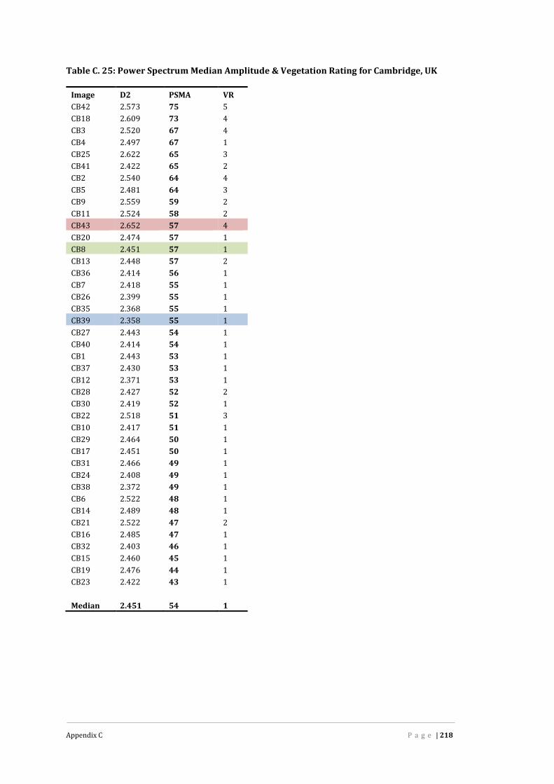
Appendix C P a g e | 218
Table C. 25: Power Spectrum Median Amplitude & Vegetation Rating for Cambridge, UK
Image D2 PSMA VRCB42 2.573 75 5CB18 2.609 73 4CB3 2.520 67 4CB4 2.497 67 1CB25 2.622 65 3CB41 2.422 65 2CB2 2.540 64 4CB5 2.481 64 3CB9 2.559 59 2CB11 2.524 58 2CB43 2.652 57 4CB20 2.474 57 1CB8 2.451 57 1CB13 2.448 57 2CB36 2.414 56 1CB7 2.418 55 1CB26 2.399 55 1CB35 2.368 55 1CB39 2.358 55 1CB27 2.443 54 1CB40 2.414 54 1CB1 2.443 53 1CB37 2.430 53 1CB12 2.371 53 1CB28 2.427 52 2CB30 2.419 52 1CB22 2.518 51 3CB10 2.417 51 1CB29 2.464 50 1CB17 2.451 50 1CB31 2.466 49 1CB24 2.408 49 1CB38 2.372 49 1CB6 2.522 48 1CB14 2.489 48 1CB21 2.522 47 2CB16 2.485 47 1CB32 2.403 46 1CB15 2.460 45 1CB19 2.476 44 1CB23 2.422 43 1Median 2.451 54 1

Appendix C P a g e | 219
Table C. 26: Power Spectrum Median Amplitude & Vegetation Rating for Central BrisbaneCity
Image D2 PSMA VR Image D2 PSMA VRCBC48 2.426 72 3 CBC13 2.325 58 4CBC26 2.512 71 4 CBC49 2.305 58 1CBC35 2.508 68 4 CBC28 2.373 57 2CBC16 2.508 68 3 CBC40 2.357 57 2CBC56 2.445 68 3 CBC11 2.354 57 2CBC50 2.438 68 2 CBC68 2.309 57 1CBC4 2.516 67 2 CBC70 2.376 56 3CBC38 2.472 66 3 CBC32 2.335 56 2CBC6 2.494 65 2 CBC37 2.455 55 1CBC21 2.468 65 3 CBC9 2.428 55 2CBC65 2.400 65 2 CBC66 2.393 55 2CBC36 2.515 64 2 CBC60 2.349 55 3CBC25 2.471 64 2 CBC55 2.406 54 1CBC5 2.462 64 2 CBC39 2.394 54 1CBC46 2.449 64 3 CBC58 2.390 54 2CBC51 2.436 64 3 CBC30 2.333 54 2CBC61 2.431 64 3 CBC63 2.328 54 2CBC20 2.416 64 1 CBC14 2.264 54 3CBC18 2.475 63 3 CBC41 2.412 53 1CBC23 2.472 63 4 CBC10 2.395 53 1CBC8 2.458 63 1 CBC7 2.383 52 1CBC19 2.448 63 2 CBC53 2.319 51 1CBC17 2.439 63 3 CBC72 2.429 49 2CBC59 2.400 63 4 CBC67 2.277 49 1CBC12 2.466 62 2 CBC29 2.227 49 3CBC54 2.461 62 2 CBC73 2.323 48 1CBC22 2.423 62 2CBC62 2.423 62 2 Median 2.418 60 2CBC24 2.391 62 2CBC42 2.440 61 3CBC45 2.426 61 2CBC31 2.391 61 4CBC57 2.376 61 3CBC71 2.328 61 3CBC69 2.482 60 3CBC1 2.459 60 2CBC15 2.450 60 2CBC27 2.380 60 3CBC52 2.435 59 3CBC2 2.421 59 2CBC47 2.410 59 2CBC3 2.389 59 2CBC44 2.387 59 3CBC43 2.439 58 2CBC33 2.412 58 2CBC34 2.384 58 3

Appendix C P a g e | 220
Table C. 27: Power Spectrum Median Amplitude & Vegetation Rating for Chermside HillsReserve, Brisbane
Image D2 PSMA VR Image D2 PSMA VRCHR17 2.665 79 5 CHR38 2.565 74 5CHR32 2.664 79 5 CHR19 2.562 74 5CHR29 2.626 79 5 CHR36 2.559 74 5CHR71 2.611 79 5 CHR52 2.555 74 5CHR3 2.572 79 5 CHR28 2.546 74 5CHR66 2.611 78 5 CHR75 2.618 73 5CHR61 2.600 78 5 CHR27 2.605 73 5CHR48 2.594 78 5 CHR8 2.550 73 4CHR41 2.631 77 5 CHR54 2.544 73 5CHR35 2.607 77 5 CHR13 2.535 73 5CHR31 2.604 77 5 CHR56 2.529 73 5CHR49 2.601 77 5 CHR63 2.528 73 5CHR64 2.598 77 5 CHR15 2.522 73 5CHR33 2.585 77 5 CHR34 2.540 72 5CHR72 2.580 77 5 CHR53 2.516 72 5CHR62 2.578 77 5 CHR65 2.507 72 5CHR60 2.533 77 5 CHR43 2.572 71 5CHR10 2.603 76 5 CHR24 2.552 71 5CHR47 2.602 76 5 CHR21 2.515 71 5CHR14 2.601 76 5 CHR69 2.491 71 5CHR26 2.597 76 5 CHR73 2.486 71 4CHR20 2.588 76 5 CHR4 2.481 71 5CHR44 2.575 76 5 CHR6 2.476 71 4CHR67 2.574 76 5 CHR46 2.526 70 5CHR74 2.570 76 5 CHR55 2.475 70 5CHR68 2.570 76 5 CHR12 2.525 69 5CHR39 2.567 76 5 CHR11 2.511 67 5CHR57 2.565 76 5 CHR70 2.508 66 4CHR1 2.559 76 5 CHR76 2.388 65 5CHR2 2.555 76 5CHR50 2.536 76 5 Median 2.567 75 5CHR58 2.525 76 5CHR25 2.648 75 5CHR22 2.595 75 5CHR42 2.590 75 5CHR18 2.588 75 5CHR7 2.556 75 5CHR45 2.555 75 5CHR9 2.544 75 5CHR37 2.523 75 5CHR77 2.518 75 5CHR16 2.591 74 5CHR40 2.589 74 5CHR30 2.589 74 5CHR23 2.586 74 5CHR51 2.582 74 5

Appendix C P a g e | 221
Table C. 28: Power Spectrum Median Amplitude & Vegetation Rating for Childers FarmLand, Queensland
Image D2 PSMA VRCFL11 2.577 67 4CFL7 2.630 65 4CFL8 2.598 65 4CFL28 2.576 65 3CFL35 2.637 64 2CFL31 2.630 64 2CFL36 2.623 64 2CFL9 2.609 64 4CFL30 2.626 63 3CFL20 2.576 62 4CFL34 2.570 62 4CFL29 2.567 62 2CFL10 2.578 61 4CFL32 2.578 61 3CFL18 2.595 59 4CFL22 2.572 59 4CFL19 2.560 58 4CFL17 2.537 58 4CFL26 2.557 57 4CFL21 2.537 57 4CFL24 2.494 57 4CFL25 2.490 57 3CFL6 2.514 54 4CFL33 2.501 54 2CFL12 2.465 54 4CFL4 2.563 53 4CFL5 2.553 53 4CFL3 2.524 53 4CFL27 2.454 53 3CFL14 2.532 52 4CFL23 2.504 52 4CFL15 2.527 51 4CFL13 2.444 51 4CFL16 2.517 50 4CFL1 2.499 50 4CFL2 2.456 49 4Median 2.558 58 4

Appendix C P a g e | 222
Table C. 29: Power Spectrum Median Amplitude & Vegetation Rating for Childers TownCentre, Queensland
Image D2 PSMA VR Image D2 PSMA RPCTC3 2.608 74 4 CTC13 2.491 60 1CTC5 2.554 74 4 CTC47 2.459 60 2CTC32 2.522 73 4 CTC27 2.403 60 4CTC44 2.465 73 4 CTC14 2.504 59 2CTC4 2.575 72 4 CTC31 2.510 57 2CTC6 2.525 72 4 CTC36 2.496 54 1CTC2 2.520 72 4CTC49 2.537 71 3 Median 2.483 67 3CTC38 2.473 71 3CTC29 2.487 70 4CTC30 2.483 70 4CTC24 2.544 69 3CTC43 2.503 69 4CTC33 2.490 69 3CTC40 2.442 69 2CTC41 2.434 69 3CTC46 2.410 69 3CTC17 2.560 68 3CTC16 2.519 68 2CTC28 2.515 68 4CTC18 2.465 68 3CTC45 2.430 68 3CTC1 2.567 67 3CTC26 2.533 67 3CTC19 2.512 67 4CTC22 2.483 67 3CTC21 2.482 67 3CTC23 2.472 67 3CTC48 2.483 66 1CTC51 2.478 66 3CTC10 2.471 66 3CTC50 2.446 66 2CTC20 2.479 65 3CTC34 2.475 65 3CTC39 2.475 65 2CTC9 2.456 65 2CTC11 2.528 64 4CTC25 2.484 64 3CTC52 2.464 64 4CTC7 2.458 64 3CTC8 2.452 64 3CTC15 2.543 63 1CTC35 2.476 63 3CTC12 2.470 63 2CTC37 2.439 63 3CTC42 2.413 63 3
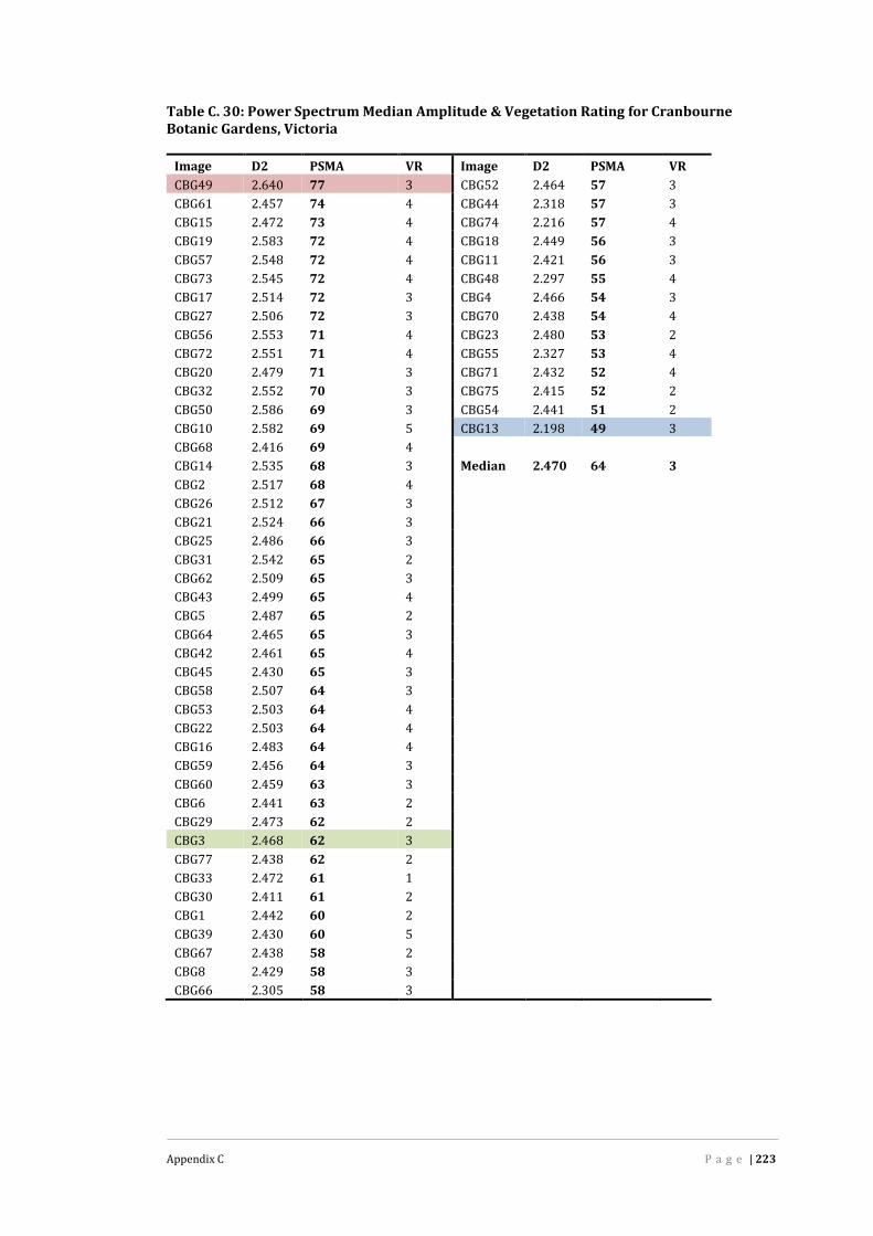
Appendix C P a g e | 223
Table C. 30: Power Spectrum Median Amplitude & Vegetation Rating for CranbourneBotanic Gardens, Victoria
Image D2 PSMA VR Image D2 PSMA VRCBG49 2.640 77 3 CBG52 2.464 57 3CBG61 2.457 74 4 CBG44 2.318 57 3CBG15 2.472 73 4 CBG74 2.216 57 4CBG19 2.583 72 4 CBG18 2.449 56 3CBG57 2.548 72 4 CBG11 2.421 56 3CBG73 2.545 72 4 CBG48 2.297 55 4CBG17 2.514 72 3 CBG4 2.466 54 3CBG27 2.506 72 3 CBG70 2.438 54 4CBG56 2.553 71 4 CBG23 2.480 53 2CBG72 2.551 71 4 CBG55 2.327 53 4CBG20 2.479 71 3 CBG71 2.432 52 4CBG32 2.552 70 3 CBG75 2.415 52 2CBG50 2.586 69 3 CBG54 2.441 51 2CBG10 2.582 69 5 CBG13 2.198 49 3CBG68 2.416 69 4CBG14 2.535 68 3 Median 2.470 64 3CBG2 2.517 68 4CBG26 2.512 67 3CBG21 2.524 66 3CBG25 2.486 66 3CBG31 2.542 65 2CBG62 2.509 65 3CBG43 2.499 65 4CBG5 2.487 65 2CBG64 2.465 65 3CBG42 2.461 65 4CBG45 2.430 65 3CBG58 2.507 64 3CBG53 2.503 64 4CBG22 2.503 64 4CBG16 2.483 64 4CBG59 2.456 64 3CBG60 2.459 63 3CBG6 2.441 63 2CBG29 2.473 62 2CBG3 2.468 62 3CBG77 2.438 62 2CBG33 2.472 61 1CBG30 2.411 61 2CBG1 2.442 60 2CBG39 2.430 60 5CBG67 2.438 58 2CBG8 2.429 58 3CBG66 2.305 58 3
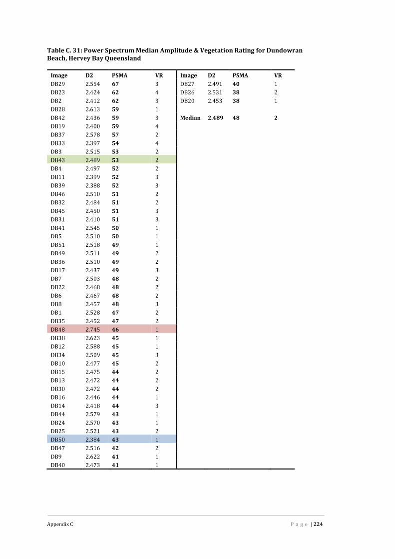
Appendix C P a g e | 224
Table C. 31: Power Spectrum Median Amplitude & Vegetation Rating for DundowranBeach, Hervey Bay Queensland
Image D2 PSMA VR Image D2 PSMA VRDB29 2.554 67 3 DB27 2.491 40 1DB23 2.424 62 4 DB26 2.531 38 2DB2 2.412 62 3 DB20 2.453 38 1DB28 2.613 59 1DB42 2.436 59 3 Median 2.489 48 2DB19 2.400 59 4DB37 2.578 57 2DB33 2.397 54 4DB3 2.515 53 2DB43 2.489 53 2DB4 2.497 52 2DB11 2.399 52 3DB39 2.388 52 3DB46 2.510 51 2DB32 2.484 51 2DB45 2.450 51 3DB31 2.410 51 3DB41 2.545 50 1DB5 2.510 50 1DB51 2.518 49 1DB49 2.511 49 2DB36 2.510 49 2DB17 2.437 49 3DB7 2.503 48 2DB22 2.468 48 2DB6 2.467 48 2DB8 2.457 48 3DB1 2.528 47 2DB35 2.452 47 2DB48 2.745 46 1DB38 2.623 45 1DB12 2.588 45 1DB34 2.509 45 3DB10 2.477 45 2DB15 2.475 44 2DB13 2.472 44 2DB30 2.472 44 2DB16 2.446 44 1DB14 2.418 44 3DB44 2.579 43 1DB24 2.570 43 1DB25 2.521 43 2DB50 2.384 43 1DB47 2.516 42 2DB9 2.622 41 1DB40 2.473 41 1

Appendix C P a g e | 225
Table C. 32: Power Spectrum Median Amplitude & Vegetation Rating for Green Park,London UK
Image D2 PSMA VRGP9 2.648 81 4GP20 2.597 81 5GP3 2.656 80 4GP11 2.639 80 5GP25 2.598 80 5GP12 2.628 79 4GP26 2.626 79 5GP21 2.624 79 5GP24 2.619 79 5GP18 2.615 78 5GP14 2.579 78 5GP10 2.591 77 4GP2 2.560 77 4GP4 2.576 76 5GP5 2.575 76 5GP13 2.535 75 4GP8 2.589 73 4GP19 2.484 73 5GP22 2.580 72 5GP17 2.452 68 5GP23 2.442 68 5GP16 2.436 62 5GP7 2.624 59 4Median 2.591 77 5

Appendix C P a g e | 226
Table C. 33: Power Spectrum Median Amplitude & Vegetation Rating for Hervey BayBotanic Gardens―Part A, Queensland
Image D2 PSMA VRHBBGa35 2.571 80 4HBBGa20 2.594 79 4HBBGa13 2.563 79 5HBBGa16 2.589 77 5HBBGa29 2.559 77 5HBBGa8 2.556 77 4HBBGa30 2.530 77 5HBBGa18 2.608 76 5HBBGa17 2.598 76 5HBBGa11 2.581 76 5HBBGa36 2.554 76 5HBBGa22 2.510 76 4HBBGa21 2.488 76 5HBBGa23 2.644 75 5HBBGa34 2.583 75 5HBBGa28 2.500 75 4HBBGa10 2.635 74 4HBBGa37 2.523 74 5HBBGa24 2.498 74 5HBBGa26 2.593 73 5HBBGa19 2.533 73 5HBBGa1 2.510 72 5HBBGa14 2.568 71 5HBBGa32 2.545 71 4HBBGa6 2.540 71 5HBBGa4 2.512 71 4HBBGa3 2.540 70 4HBBGa5 2.522 70 4HBBGa15 2.437 70 5HBBGa9 2.590 69 4HBBGa33 2.538 69 4HBBGa25 2.412 69 5HBBGa31 2.513 68 5HBBGa12 2.510 68 4HBBGa27 2.444 68 5HBBGa2 2.475 67 4HBBGa7 2.350 62 4Median 2.350 62 4

Appendix C P a g e | 227
Table C. 34: Power Spectrum Median Amplitude & Vegetation Rating for Hervey BayBotanic Gardens―Part B, Queensland
Image D2 PSMA VRHBBGb11 2.633 84 5HBBGb8 2.620 83 5HBBGb12 2.636 82 5HBBGb4 2.618 82 5HBBGb32 2.615 82 5HBBGb10 2.599 82 5HBBGb19 2.597 82 5HBBGb6 2.612 81 5HBBGb15 2.611 81 5HBBGb7 2.609 81 5HBBGb13 2.591 81 5HBBGb2 2.581 81 5HBBGb14 2.577 81 5HBBGb24 2.573 81 5HBBGb21 2.629 80 5HBBGb20 2.581 80 5HBBGb9 2.579 80 5HBBGb3 2.578 80 5HBBGb16 2.576 79 5HBBGb5 2.570 79 5HBBGb23 2.581 78 5HBBGb28 2.527 78 5HBBGb31 2.596 77 5HBBGb26 2.534 77 5HBBGb1 2.531 77 5HBBGb17 2.527 77 5HBBGb33 2.573 76 5HBBGb18 2.519 76 5HBBGb25 2.528 75 4HBBGb22 2.521 75 4HBBGb30 2.523 74 5HBBGb27 2.456 74 5HBBGb29 2.460 73 5Median 2.579 80 5

Appendix C P a g e | 228
Table C. 35: Power Spectrum Median Amplitude & Vegetation Rating for Hervey BayEsplanade, Queensland
Image D2 PSMA VR Image D2 PSMA VRHBE12 2.575 76 4 HBE27 2.476 62 3HBE13 2.523 76 5 HBE9 2.450 62 4HBE14 2.569 75 5 HBE44 2.421 62 4HBE8 2.511 74 5 HBE57 2.406 62 4HBE2 2.583 73 5 HBE45 2.390 61 3HBE53 2.555 73 4 HBE47 2.475 60 2HBE1 2.535 73 4 HBE5 2.440 60 3HBE11 2.495 73 4 HBE17 2.523 58 2HBE15 2.503 72 5 HBE56 2.448 57 4HBE7 2.497 72 5 HBE58 2.448 55 3HBE38 2.547 71 4 HBE4 2.403 54 2HBE6 2.530 71 4 HBE50 2.323 54 4HBE55 2.515 71 4HBE20 2.501 71 5 Median 2.476 66 4HBE16 2.498 71 4HBE34 2.448 71 4HBE49 2.458 70 4HBE54 2.452 70 5HBE10 2.489 69 4HBE39 2.460 69 4HBE35 2.430 69 4HBE25 2.512 67 4HBE26 2.494 67 4HBE37 2.478 67 5HBE28 2.476 67 4HBE43 2.429 67 4HBE31 2.532 66 3HBE30 2.504 66 4HBE36 2.501 66 5HBE40 2.467 66 3HBE23 2.464 66 4HBE32 2.448 66 4HBE52 2.425 66 4HBE33 2.511 65 3HBE19 2.493 65 4HBE18 2.460 65 4HBE41 2.500 64 3HBE22 2.470 64 4HBE51 2.466 64 4HBE48 2.448 64 4HBE3 2.443 64 3HBE46 2.435 64 3HBE21 2.419 64 4HBE42 2.395 64 4HBE24 2.550 62 3HBE29 2.478 62 3
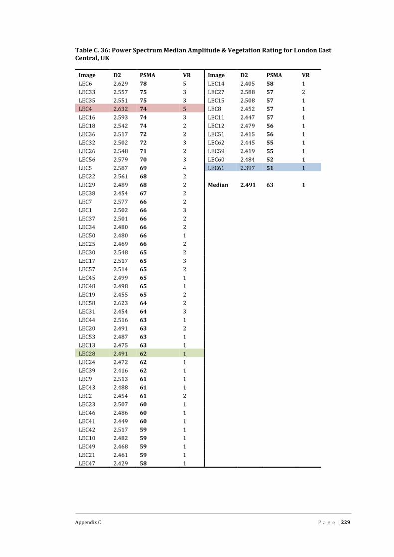
Appendix C P a g e | 229
Table C. 36: Power Spectrum Median Amplitude & Vegetation Rating for London EastCentral, UK
Image D2 PSMA VR Image D2 PSMA VRLEC6 2.629 78 5 LEC14 2.405 58 1LEC33 2.557 75 3 LEC27 2.588 57 2LEC35 2.551 75 3 LEC15 2.508 57 1LEC4 2.632 74 5 LEC8 2.452 57 1LEC16 2.593 74 3 LEC11 2.447 57 1LEC18 2.542 74 2 LEC12 2.479 56 1LEC36 2.517 72 2 LEC51 2.415 56 1LEC32 2.502 72 3 LEC62 2.445 55 1LEC26 2.548 71 2 LEC59 2.419 55 1LEC56 2.579 70 3 LEC60 2.484 52 1LEC5 2.587 69 4 LEC61 2.397 51 1LEC22 2.561 68 2LEC29 2.489 68 2 Median 2.491 63 1LEC38 2.454 67 2LEC7 2.577 66 2LEC1 2.502 66 3LEC37 2.501 66 2LEC34 2.480 66 2LEC50 2.480 66 1LEC25 2.469 66 2LEC30 2.548 65 2LEC17 2.517 65 3LEC57 2.514 65 2LEC45 2.499 65 1LEC48 2.498 65 1LEC19 2.455 65 2LEC58 2.623 64 2LEC31 2.454 64 3LEC44 2.516 63 1LEC20 2.491 63 2LEC53 2.487 63 1LEC13 2.475 63 1LEC28 2.491 62 1LEC24 2.472 62 1LEC39 2.416 62 1LEC9 2.513 61 1LEC43 2.488 61 1LEC2 2.454 61 2LEC23 2.507 60 1LEC46 2.486 60 1LEC41 2.449 60 1LEC42 2.517 59 1LEC10 2.482 59 1LEC49 2.468 59 1LEC21 2.461 59 1LEC47 2.429 58 1

Appendix C P a g e | 230
Table C. 37: Power Spectrum Median Amplitude & Vegetation Rating for London WestOne, UK
Image D2 PSMA VR Image D2 PSMA VRLW85 2.627 80 5 LW68 2.401 58 1LW84 2.616 80 5 LW57 2.375 58 1LW78 2.614 78 4 LW60 2.346 58 2LW92 2.541 78 3 LW82 2.277 58 2LW94 2.594 76 5 LW77 2.416 57 1LW79 2.573 76 5 LW63 2.413 57 1LW10 2.544 76 2 LW28 2.368 57 1LW9 2.595 75 4 LW61 2.364 57 1LW13 2.496 75 4 LW20 2.516 56 1LW14 2.441 75 3 LW18 2.428 56 1LW39 2.544 72 4 LW3 2.406 56 1LW6 2.541 72 3 LW16 2.404 56 1LW7 2.518 72 3 LW50 2.386 56 1LW70 2.493 72 2 LW44 2.368 56 1LW15 2.477 72 2 LW41 2.493 55 1LW81 2.453 72 3 LW56 2.432 55 1LW40 2.461 71 2 LW26 2.423 55 1LW93 2.545 68 2 LW27 2.409 55 1LW4 2.450 68 2 LW21 2.389 55 1LW55 2.393 68 2 LW86 2.377 55 1LW80 2.526 67 4 LW29 2.352 55 1LW59 2.524 67 2 LW62 2.347 55 1LW54 2.476 67 2 LW65 2.344 55 1LW45 2.446 67 2 LW46 2.339 55 1LW11 2.433 65 5 LW53 2.323 55 1LW91 2.529 64 1 LW12 2.471 54 3LW96 2.474 64 1 LW22 2.417 54 1LW48 2.445 64 2 LW1 2.415 54 1LW90 2.421 64 1 LW69 2.402 54 1LW71 2.384 64 2 LW72 2.323 54 2LW36 2.473 63 1 LW30 2.323 54 1LW95 2.431 62 1 LW64 2.279 54 1LW76 2.421 62 2 LW73 2.324 53 2LW67 2.461 61 1 LW51 2.323 53 1LW8 2.462 60 2 LW34 2.318 53 1LW25 2.402 60 1 LW75 2.305 53 1LW5 2.393 60 2 LW42 2.348 52 1LW83 2.465 59 1 LW66 2.297 51 1LW24 2.457 59 1 LW52 2.280 51 1LW38 2.410 59 1 LW74 2.184 51 1LW17 2.402 59 1 LW58 2.324 50 1LW49 2.398 59 1 LW31 2.266 50 1LW47 2.381 59 1 LW37 2.158 50 1LW19 2.437 58 1 LW2 2.489 48 1LW23 2.412 58 1 LW43 2.179 47 1LW35 2.403 58 1Median 2.415 58 1

Appendix C P a g e | 231
Table C. 38: Power Spectrum Median Amplitude & Vegetation Rating for MelbourneDocklands, Victoria
Image D2 PSMA VRMD34 2.405 59 1MD35 2.425 58 2MD7 2.498 57 1MD38 2.417 57 1MD32 2.324 57 3MD39 2.368 56 1MD6 2.496 55 1MD4 2.401 55 1MD19 2.433 54 1MD12 2.431 54 2MD36 2.403 54 2MD24 2.434 53 1MD13 2.493 52 3MD18 2.486 52 1MD5 2.417 52 1MD15 2.408 52 1MD31 2.396 52 2MD22 2.383 52 1MD11 2.460 51 1MD16 2.381 51 1MD17 2.378 51 2MD14 2.361 51 2MD37 2.457 50 2MD20 2.402 50 1MD21 2.313 50 1MD9 2.450 49 2MD28 2.426 49 1MD1 2.409 49 1MD29 2.394 49 1MD8 2.305 49 1MD3 2.548 48 1MD26 2.475 48 1MD23 2.409 48 1MD30 2.363 48 2MD2 2.488 47 1MD27 2.474 47 1MD10 2.452 47 1MD33 2.392 47 1Median 2.413 51 1

Appendix C P a g e | 232
Table C. 39: Power Spectrum Median Amplitude & Vegetation Rating for Regents Park,London UK
Image D2 PSMA VR Image D2 PSMA VRRP44 2.639 81 4 RP42 2.632 62 4RP61 2.657 80 4 RP52 2.577 62 4RP3 2.602 78 4 RP33 2.623 61 4RP59 2.649 77 5 RP40 2.565 61 4RP16 2.645 77 4 RP26 2.579 60 3RP45 2.640 77 5 RP39 2.602 58 4RP17 2.624 77 5 RP15 2.622 57 3RP37 2.620 77 5 RP18 2.599 57 3RP2 2.663 76 4 RP11 2.590 56 3RP46 2.574 76 5 RP14 2.572 55 3RP7 2.664 75 4 RP22 2.641 54 2RP29 2.645 75 4RP5 2.644 75 4 Median 2.614 70 4RP6 2.663 74 4RP23 2.617 74 4RP36 2.614 74 5RP28 2.580 74 4RP27 2.566 74 4RP55 2.619 73 4RP47 2.614 73 5RP63 2.580 73 5RP1 2.653 71 4RP56 2.618 71 3RP43 2.597 71 4RP51 2.587 71 4RP8 2.583 71 4RP30 2.546 71 4RP57 2.530 71 5RP34 2.662 70 4RP64 2.654 69 5RP60 2.645 69 4RP4 2.596 69 4RP62 2.554 69 4RP38 2.508 69 5RP48 2.651 68 4RP35 2.591 68 4RP31 2.655 67 4RP54 2.634 67 4RP41 2.609 67 5RP24 2.589 67 4RP10 2.615 66 3RP53 2.537 66 4RP9 2.615 65 3RP49 2.595 65 4RP25 2.579 63 3RP58 2.563 63 4

Appendix C P a g e | 233
Table C. 40: Power Spectrum Median Amplitude & Vegetation Rating for Roma StreetParklands, Brisbane
Image D2 PSMA VR Image D2 PSMA VRRSP78 2.582 77 5 RSP77 2.442 69 5RSP73 2.553 77 5 RSP81 2.570 68 4RSP32 2.621 76 4 RSP45 2.556 68 4RSP12 2.558 76 5 RSP53 2.555 68 4RSP41 2.605 75 4 RSP20 2.539 68 4RSP79 2.571 75 4 RSP10 2.507 68 2RSP60 2.571 75 5 RSP17 2.485 68 3RSP8 2.559 75 4 RSP63 2.482 68 4RSP76 2.556 75 5 RSP1 2.475 68 3RSP23 2.506 75 5 RSP5 2.468 68 4RSP31 2.505 75 4 RSP62 2.461 68 5RSP90 2.613 74 5 RSP67 2.559 67 3RSP68 2.573 74 5 RSP84 2.554 67 4RSP13 2.566 74 5 RSP42 2.529 67 4RSP25 2.516 74 5 RSP91 2.516 67 4RSP7 2.505 74 5 RSP6 2.484 67 4RSP69 2.591 73 4 RSP2 2.454 67 3RSP47 2.568 73 5 RSP18 2.447 67 5RSP75 2.558 73 4 RSP16 2.525 66 5RSP38 2.541 73 3 RSP21 2.520 66 4RSP56 2.558 72 4 RSP71 2.488 66 5RSP39 2.553 72 3 RSP34 2.484 66 3RSP54 2.529 72 5 RSP27 2.478 66 3RSP92 2.501 72 4 RSP24 2.444 66 3RSP22 2.574 71 4 RSP33 2.433 66 4RSP65 2.549 71 4 RSP11 2.428 66 5RSP30 2.549 71 4 RSP93 2.465 65 3RSP59 2.548 71 4 RSP64 2.438 65 4RSP80 2.545 71 4 RSP58 2.432 65 5RSP87 2.529 71 4 RSP70 2.419 65 5RSP82 2.561 70 4 RSP46 2.521 64 4RSP49 2.551 70 4 RSP29 2.481 64 3RSP85 2.540 70 4 RSP15 2.458 64 4RSP37 2.532 70 4 RSP3 2.447 64 3RSP72 2.527 70 5 RSP19 2.487 63 3RSP52 2.519 70 5 RSP43 2.463 63 3RSP57 2.500 70 5 RSP96 2.457 63 1RSP74 2.497 70 4 RSP61 2.425 63 4RSP55 2.494 70 5 RSP95 2.418 63 3RSP36 2.486 70 4 RSP86 2.502 60 4RSP14 2.485 70 5 RSP4 2.453 59 3RSP51 2.466 70 5 RSP89 2.412 58 3RSP83 2.448 70 5 RSP40 2.506 57 2RSP66 2.446 70 5 RSP26 2.427 57 2RSP48 2.533 69 4 RSP88 2.450 56 2RSP9 2.502 69 4 RSP50 2.214 47 1RSP44 2.500 69 5 RSP28 2.134 44 3RSP94 2.479 69 4RSP35 2.463 69 4 Median 2.505 69 4
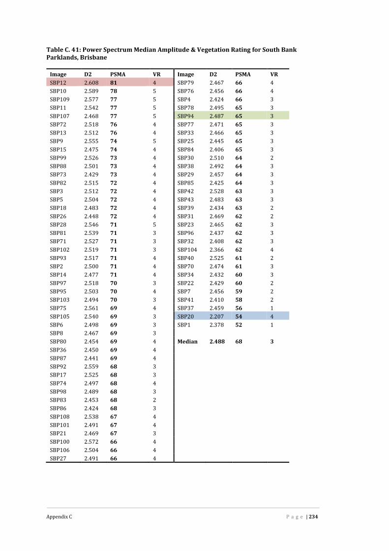
Appendix C P a g e | 234
Table C. 41: Power Spectrum Median Amplitude & Vegetation Rating for South BankParklands, Brisbane
Image D2 PSMA VR Image D2 PSMA VRSBP12 2.608 81 4 SBP79 2.467 66 4SBP10 2.589 78 5 SBP76 2.456 66 4SBP109 2.577 77 5 SBP4 2.424 66 3SBP11 2.542 77 5 SBP78 2.495 65 3SBP107 2.468 77 5 SBP94 2.487 65 3SBP72 2.518 76 4 SBP77 2.471 65 3SBP13 2.512 76 4 SBP33 2.466 65 3SBP9 2.555 74 5 SBP25 2.445 65 3SBP15 2.475 74 4 SBP84 2.406 65 3SBP99 2.526 73 4 SBP30 2.510 64 2SBP88 2.501 73 4 SBP38 2.492 64 3SBP73 2.429 73 4 SBP29 2.457 64 3SBP82 2.515 72 4 SBP85 2.425 64 3SBP3 2.512 72 4 SBP42 2.528 63 3SBP5 2.504 72 4 SBP43 2.483 63 3SBP18 2.483 72 4 SBP39 2.434 63 2SBP26 2.448 72 4 SBP31 2.469 62 2SBP28 2.546 71 5 SBP23 2.465 62 3SBP81 2.539 71 3 SBP96 2.437 62 3SBP71 2.527 71 3 SBP32 2.408 62 3SBP102 2.519 71 3 SBP104 2.366 62 4SBP93 2.517 71 4 SBP40 2.525 61 2SBP2 2.500 71 4 SBP70 2.474 61 3SBP14 2.477 71 4 SBP34 2.432 60 3SBP97 2.518 70 3 SBP22 2.429 60 2SBP95 2.503 70 4 SBP7 2.456 59 2SBP103 2.494 70 3 SBP41 2.410 58 2SBP75 2.561 69 4 SBP37 2.459 56 1SBP105 2.540 69 3 SBP20 2.207 54 4SBP6 2.498 69 3 SBP1 2.378 52 1SBP8 2.467 69 3SBP80 2.454 69 4 Median 2.488 68 3SBP36 2.450 69 4SBP87 2.441 69 4SBP92 2.559 68 3SBP17 2.525 68 3SBP74 2.497 68 4SBP98 2.489 68 3SBP83 2.453 68 2SBP86 2.424 68 3SBP108 2.538 67 4SBP101 2.491 67 4SBP21 2.469 67 3SBP100 2.572 66 4SBP106 2.504 66 4SBP27 2.491 66 4

Appendix C P a g e | 235
Table C. 42: Power Spectrum Median Amplitude & Vegetation Rating for St James Park,London UK
Image D2 PSMA VRStJP8 2.568 80 5StJP2 2.622 79 5StJP3 2.600 79 5StJP13 2.626 78 5StJP9 2.586 78 5StJP17 2.662 76 5StJP6 2.597 76 5StJP18 2.689 75 4StJP10 2.536 75 5StJP15 2.657 74 4StJP14 2.634 74 5StJP16 2.604 74 5StJP20 2.617 73 3StJP7 2.659 72 4StJP12 2.458 71 5StJP4 2.574 70 4StJP21 2.582 69 5StJP5 2.615 66 4StJP1 2.431 66 5StJP22 2.362 65 5StJP19 2.620 63 3StJP11 2.593 63 3Median 2.602 74 5

Appendix C P a g e | 236
Table C. 43: PSMA & VR Rating for Toowoomba City Centre, Queensland
Image D2 PSMA VR Image D2 PSMA VRTCC12 2.527 72 4 TCC1 2.507 57 1TCC31 2.515 72 3 TCC40 2.477 57 1TCC32 2.533 70 4 TCC13 2.425 57 1TCC21 2.455 68 4 TCC46 2.393 56 2TCC7 2.558 67 1 TCC28 2.376 56 2TCC27 2.469 66 4 TCC39 2.488 55 1TCC5 2.412 66 4 TCC19 2.465 55 1TCC36 2.420 65 1 TCC24 2.398 55 2TCC6 2.450 64 3TCC43 2.442 64 3 Median 2.458 59 2TCC15 2.416 64 3TCC49 2.510 63 2TCC22 2.498 63 2TCC11 2.429 63 2TCC4 2.380 63 3TCC50 2.396 62 2TCC17 2.380 62 3TCC8 2.495 61 1TCC44 2.408 61 1TCC38 2.497 60 3TCC37 2.458 60 2TCC16 2.416 60 1TCC48 2.407 60 2TCC23 2.403 60 2TCC29 2.390 60 1TCC25 2.520 59 2TCC42 2.503 59 1TCC35 2.477 59 1TCC41 2.472 59 1TCC20 2.471 59 2TCC10 2.467 59 1TCC2 2.419 59 1TCC9 2.507 58 1TCC30 2.506 58 2TCC47 2.493 58 1TCC26 2.489 58 2TCC51 2.466 58 1TCC18 2.437 58 1TCC3 2.392 58 1TCC33 2.381 58 1TCC14 2.368 58 2TCC45 2.356 58 1TCC34 2.534 57 1
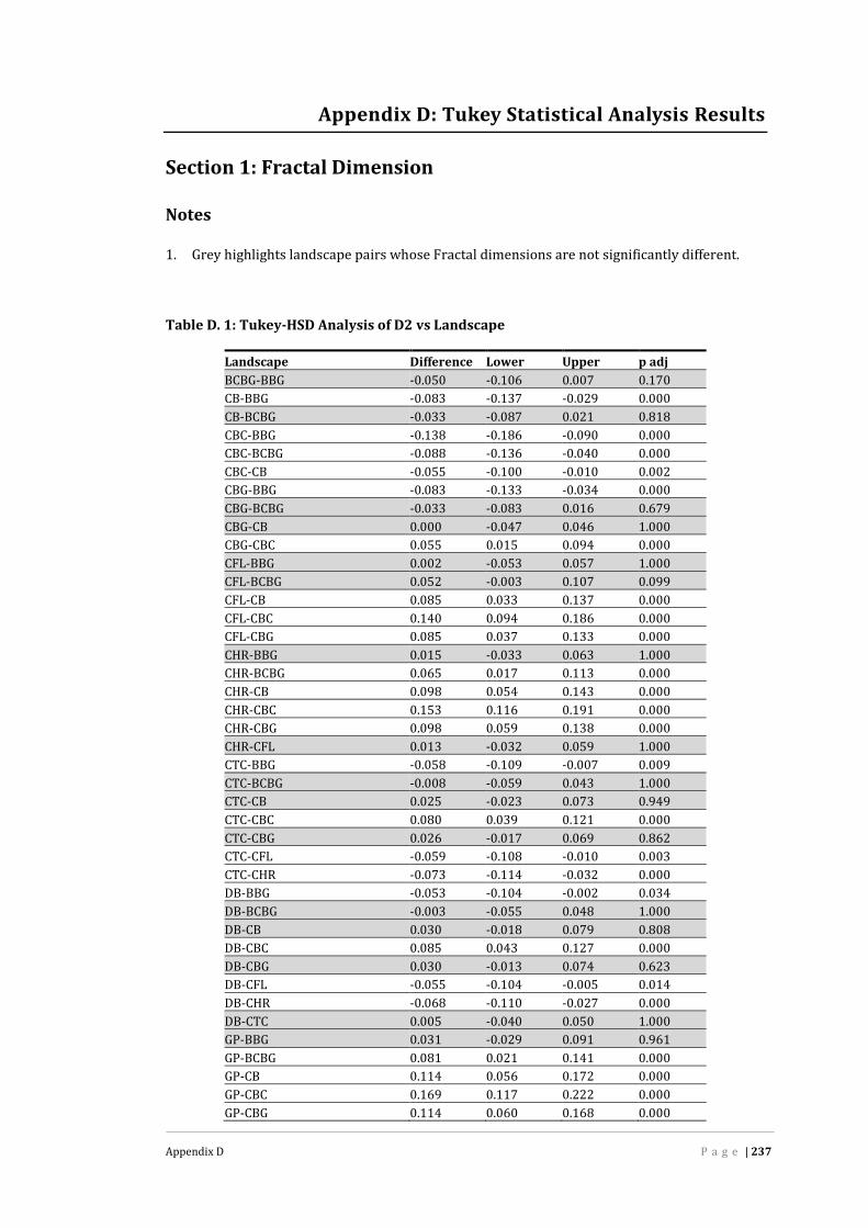
Appendix D P a g e | 237
Appendix D: Tukey Statistical Analysis Results
Section 1: Fractal Dimension
Notes1. Grey highlights landscape pairs whose Fractal dimensions are not significantly different.Table D. 1: Tukey-HSD Analysis of D2 vs Landscape
Landscape Difference Lower Upper p adjBCBG-BBG -0.050 -0.106 0.007 0.170CB-BBG -0.083 -0.137 -0.029 0.000CB-BCBG -0.033 -0.087 0.021 0.818CBC-BBG -0.138 -0.186 -0.090 0.000CBC-BCBG -0.088 -0.136 -0.040 0.000CBC-CB -0.055 -0.100 -0.010 0.002CBG-BBG -0.083 -0.133 -0.034 0.000CBG-BCBG -0.033 -0.083 0.016 0.679CBG-CB 0.000 -0.047 0.046 1.000CBG-CBC 0.055 0.015 0.094 0.000CFL-BBG 0.002 -0.053 0.057 1.000CFL-BCBG 0.052 -0.003 0.107 0.099CFL-CB 0.085 0.033 0.137 0.000CFL-CBC 0.140 0.094 0.186 0.000CFL-CBG 0.085 0.037 0.133 0.000CHR-BBG 0.015 -0.033 0.063 1.000CHR-BCBG 0.065 0.017 0.113 0.000CHR-CB 0.098 0.054 0.143 0.000CHR-CBC 0.153 0.116 0.191 0.000CHR-CBG 0.098 0.059 0.138 0.000CHR-CFL 0.013 -0.032 0.059 1.000CTC-BBG -0.058 -0.109 -0.007 0.009CTC-BCBG -0.008 -0.059 0.043 1.000CTC-CB 0.025 -0.023 0.073 0.949CTC-CBC 0.080 0.039 0.121 0.000CTC-CBG 0.026 -0.017 0.069 0.862CTC-CFL -0.059 -0.108 -0.010 0.003CTC-CHR -0.073 -0.114 -0.032 0.000DB-BBG -0.053 -0.104 -0.002 0.034DB-BCBG -0.003 -0.055 0.048 1.000DB-CB 0.030 -0.018 0.079 0.808DB-CBC 0.085 0.043 0.127 0.000DB-CBG 0.030 -0.013 0.074 0.623DB-CFL -0.055 -0.104 -0.005 0.014DB-CHR -0.068 -0.110 -0.027 0.000DB-CTC 0.005 -0.040 0.050 1.000GP-BBG 0.031 -0.029 0.091 0.961GP-BCBG 0.081 0.021 0.141 0.000GP-CB 0.114 0.056 0.172 0.000GP-CBC 0.169 0.117 0.222 0.000GP-CBG 0.114 0.060 0.168 0.000
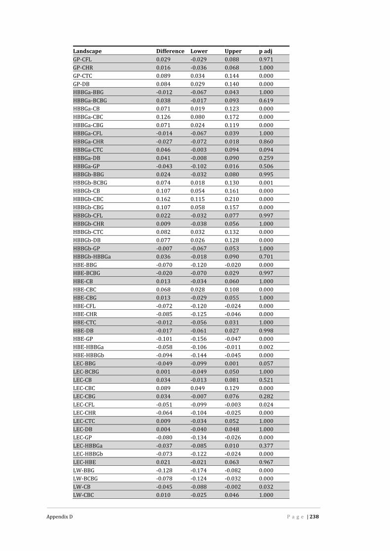
Appendix D P a g e | 238
Landscape Difference Lower Upper p adjGP-CFL 0.029 -0.029 0.088 0.971GP-CHR 0.016 -0.036 0.068 1.000GP-CTC 0.089 0.034 0.144 0.000GP-DB 0.084 0.029 0.140 0.000HBBGa-BBG -0.012 -0.067 0.043 1.000HBBGa-BCBG 0.038 -0.017 0.093 0.619HBBGa-CB 0.071 0.019 0.123 0.000HBBGa-CBC 0.126 0.080 0.172 0.000HBBGa-CBG 0.071 0.024 0.119 0.000HBBGa-CFL -0.014 -0.067 0.039 1.000HBBGa-CHR -0.027 -0.072 0.018 0.860HBBGa-CTC 0.046 -0.003 0.094 0.094HBBGa-DB 0.041 -0.008 0.090 0.259HBBGa-GP -0.043 -0.102 0.016 0.506HBBGb-BBG 0.024 -0.032 0.080 0.995HBBGb-BCBG 0.074 0.018 0.130 0.001HBBGb-CB 0.107 0.054 0.161 0.000HBBGb-CBC 0.162 0.115 0.210 0.000HBBGb-CBG 0.107 0.058 0.157 0.000HBBGb-CFL 0.022 -0.032 0.077 0.997HBBGb-CHR 0.009 -0.038 0.056 1.000HBBGb-CTC 0.082 0.032 0.132 0.000HBBGb-DB 0.077 0.026 0.128 0.000HBBGb-GP -0.007 -0.067 0.053 1.000HBBGb-HBBGa 0.036 -0.018 0.090 0.701HBE-BBG -0.070 -0.120 -0.020 0.000HBE-BCBG -0.020 -0.070 0.029 0.997HBE-CB 0.013 -0.034 0.060 1.000HBE-CBC 0.068 0.028 0.108 0.000HBE-CBG 0.013 -0.029 0.055 1.000HBE-CFL -0.072 -0.120 -0.024 0.000HBE-CHR -0.085 -0.125 -0.046 0.000HBE-CTC -0.012 -0.056 0.031 1.000HBE-DB -0.017 -0.061 0.027 0.998HBE-GP -0.101 -0.156 -0.047 0.000HBE-HBBGa -0.058 -0.106 -0.011 0.002HBE-HBBGb -0.094 -0.144 -0.045 0.000LEC-BBG -0.049 -0.099 0.001 0.057LEC-BCBG 0.001 -0.049 0.050 1.000LEC-CB 0.034 -0.013 0.081 0.521LEC-CBC 0.089 0.049 0.129 0.000LEC-CBG 0.034 -0.007 0.076 0.282LEC-CFL -0.051 -0.099 -0.003 0.024LEC-CHR -0.064 -0.104 -0.025 0.000LEC-CTC 0.009 -0.034 0.052 1.000LEC-DB 0.004 -0.040 0.048 1.000LEC-GP -0.080 -0.134 -0.026 0.000LEC-HBBGa -0.037 -0.085 0.010 0.377LEC-HBBGb -0.073 -0.122 -0.024 0.000LEC-HBE 0.021 -0.021 0.063 0.967LW-BBG -0.128 -0.174 -0.082 0.000LW-BCBG -0.078 -0.124 -0.032 0.000LW-CB -0.045 -0.088 -0.002 0.032LW-CBC 0.010 -0.025 0.046 1.000

Appendix D P a g e | 239
Landscape Difference Lower Upper p adjLW-CBG -0.045 -0.082 -0.007 0.004LW-CFL -0.130 -0.174 -0.085 0.000LW-CHR -0.143 -0.178 -0.108 0.000LW-CTC -0.070 -0.109 -0.031 0.000LW-DB -0.075 -0.115 -0.035 0.000LW-GP -0.159 -0.210 -0.108 0.000LW-HBBGa -0.116 -0.160 -0.072 0.000LW-HBBGb -0.152 -0.198 -0.106 0.000LW-HBE -0.058 -0.096 -0.020 0.000LW-LEC -0.079 -0.117 -0.041 0.000MD-BBG -0.127 -0.182 -0.073 0.000MD-BCBG -0.077 -0.132 -0.023 0.000MD-CB -0.044 -0.096 0.008 0.226MD-CBC 0.011 -0.035 0.057 1.000MD-CBG -0.044 -0.091 0.004 0.112MD-CFL -0.129 -0.182 -0.076 0.000MD-CHR -0.142 -0.188 -0.097 0.000MD-CTC -0.069 -0.118 -0.021 0.000MD-DB -0.074 -0.124 -0.025 0.000MD-GP -0.158 -0.217 -0.100 0.000MD-HBBGa -0.115 -0.168 -0.063 0.000MD-HBBGb -0.151 -0.205 -0.097 0.000MD-HBE -0.057 -0.105 -0.009 0.004MD-LEC -0.078 -0.126 -0.031 0.000MD-LW 0.001 -0.043 0.045 1.000RP-BBG 0.062 0.013 0.112 0.002RP-BCBG 0.112 0.063 0.162 0.000RP-CB 0.146 0.099 0.192 0.000RP-CBC 0.201 0.161 0.240 0.000RP-CBG 0.146 0.104 0.188 0.000RP-CFL 0.061 0.013 0.109 0.001RP-CHR 0.047 0.008 0.087 0.004RP-CTC 0.120 0.077 0.163 0.000RP-DB 0.115 0.072 0.159 0.000RP-GP 0.031 -0.023 0.085 0.886RP-HBBGa 0.074 0.027 0.122 0.000RP-HBBGb 0.038 -0.011 0.088 0.388RP-HBE 0.133 0.091 0.175 0.000RP-LEC 0.112 0.070 0.153 0.000RP-LW 0.190 0.152 0.228 0.000RP-MD 0.190 0.142 0.237 0.000RSP-BBG -0.047 -0.093 -0.001 0.044RSP-BCBG 0.003 -0.043 0.049 1.000RSP-CB 0.036 -0.007 0.079 0.230RSP-CBC 0.091 0.056 0.127 0.000RSP-CBG 0.037 -0.001 0.074 0.064RSP-CFL -0.048 -0.093 -0.004 0.015RSP-CHR -0.062 -0.097 -0.027 0.000RSP-CTC 0.011 -0.028 0.050 1.000RSP-DB 0.006 -0.033 0.046 1.000RSP-GP -0.078 -0.129 -0.027 0.000RSP-HBBGa -0.035 -0.079 0.009 0.349RSP-HBBGb -0.071 -0.116 -0.025 0.000RSP-HBE 0.024 -0.014 0.061 0.795

Appendix D P a g e | 240
Landscape Difference Lower Upper p adjRSP-LEC 0.002 -0.035 0.040 1.000RSP-LW 0.081 0.048 0.114 0.000RSP-MD 0.081 0.037 0.124 0.000RSP-RP -0.109 -0.147 -0.072 0.000SBP-BBG -0.065 -0.112 -0.017 0.000SBP-BCBG -0.015 -0.063 0.033 1.000SBP-CB 0.018 -0.026 0.063 0.997SBP-CBC 0.073 0.036 0.111 0.000SBP-CBG 0.019 -0.021 0.058 0.985SBP-CFL -0.066 -0.112 -0.021 0.000SBP-CHR -0.080 -0.117 -0.043 0.000SBP-CTC -0.007 -0.048 0.034 1.000SBP-DB -0.012 -0.053 0.030 1.000SBP-GP -0.096 -0.148 -0.044 0.000SBP-HBBGa -0.053 -0.098 -0.008 0.006SBP-HBBGb -0.089 -0.136 -0.042 0.000SBP-HBE 0.005 -0.034 0.045 1.000SBP-LEC -0.016 -0.055 0.024 0.998SBP-LW 0.063 0.028 0.098 0.000SBP-MD 0.062 0.017 0.108 0.000SBP-RP -0.127 -0.167 -0.088 0.000SBP-RSP -0.018 -0.053 0.017 0.956StJP-BBG 0.039 -0.024 0.101 0.819StJP-BCBG 0.088 0.026 0.151 0.000StJP-CB 0.122 0.061 0.182 0.000StJP-CBC 0.177 0.122 0.232 0.000StJP-CBG 0.122 0.065 0.178 0.000StJP-CFL 0.037 -0.024 0.098 0.844StJP-CHR 0.023 -0.031 0.078 0.995StJP-CTC 0.096 0.039 0.154 0.000StJP-DB 0.092 0.034 0.150 0.000StJP-GP 0.007 -0.059 0.074 1.000StJP-HBBGa 0.051 -0.010 0.111 0.268StJP-HBBGb 0.015 -0.048 0.077 1.000StJP-HBE 0.109 0.052 0.165 0.000StJP-LEC 0.088 0.031 0.144 0.000StJP-LW 0.167 0.113 0.220 0.000StJP-MD 0.166 0.105 0.227 0.000StJP-RP -0.024 -0.081 0.033 0.996StJP-RSP 0.085 0.032 0.139 0.000StJP-SBP 0.103 0.049 0.158 0.000TCC-BBG -0.095 -0.146 -0.044 0.000TCC-BCBG -0.046 -0.097 0.005 0.154TCC-CB -0.012 -0.060 0.036 1.000TCC-CBC 0.043 0.001 0.084 0.035TCC-CBG -0.012 -0.055 0.031 1.000TCC-CFL -0.097 -0.146 -0.048 0.000TCC-CHR -0.111 -0.152 -0.069 0.000TCC-CTC -0.038 -0.082 0.007 0.236TCC-DB -0.042 -0.088 0.003 0.099TCC-GP -0.127 -0.182 -0.071 0.000TCC-HBBGa -0.084 -0.132 -0.035 0.000TCC-HBBGb -0.120 -0.170 -0.069 0.000TCC-HBE -0.025 -0.069 0.018 0.885

Appendix D P a g e | 241
Landscape Difference Lower Upper p adjTCC-LEC -0.046 -0.090 -0.003 0.020TCC-LW 0.032 -0.007 0.072 0.282TCC-MD 0.032 -0.017 0.081 0.736TCC-RP -0.158 -0.201 -0.114 0.000TCC-RSP -0.049 -0.088 -0.010 0.002TCC-SBP -0.031 -0.072 0.010 0.468TCC-StJP -0.134 -0.192 -0.076 0.000

Appendix D P a g e | 242
Section 2: Power Spectrum Median Amplitude
Notes1. Grey highlights landscape pairs whose PSMA are not significantly different.Table D. 2: Tukey-HSD Analysis for PSMA vs Landscape
Landscape Difference Lower Upper p adjBCBG-BBG -4.094 -9.219 1.031 0.337CB-BBG -19.415 -24.305 -14.526 0.000CB-BCBG -15.321 -20.211 -10.432 0.000CBC-BBG -14.632 -18.987 -10.277 0.000CBC-BCBG -10.538 -14.894 -6.183 0.000CBC-CB 4.783 0.707 8.859 0.005CBG-BBG -11.160 -15.660 -6.659 0.000CBG-BCBG -7.066 -11.567 -2.566 0.000CBG-CB 8.255 4.025 12.486 0.000CBG-CBC 3.472 -0.128 7.072 0.075CFL-BBG -16.535 -21.515 -11.554 0.000CFL-BCBG -12.441 -17.421 -7.460 0.000CFL-CB 2.880 -1.858 7.618 0.834CFL-CBC -1.903 -6.087 2.282 0.990CFL-CBG -5.375 -9.710 -1.039 0.002CHR-BBG -0.139 -4.468 4.189 1.000CHR-BCBG 3.955 -0.374 8.283 0.127CHR-CB 19.276 15.229 23.323 0.000CHR-CBC 14.493 11.111 17.875 0.000CHR-CBG 11.021 7.453 14.588 0.000CHR-CFL 16.396 12.239 20.552 0.000CTC-BBG -7.832 -12.438 -3.226 0.000CTC-BCBG -3.738 -8.344 0.868 0.307CTC-CB 11.583 7.241 15.926 0.000CTC-CBC 6.800 3.070 10.531 0.000CTC-CBG 3.328 -0.571 7.227 0.220CTC-CFL 8.703 4.258 13.148 0.000CTC-CHR -7.693 -11.392 -3.993 0.000DB-BBG -25.639 -30.298 -20.980 0.000DB-BCBG -21.545 -26.205 -16.886 0.000DB-CB -6.224 -10.623 -1.825 0.000DB-CBC -11.007 -14.803 -7.211 0.000DB-CBG -14.479 -18.441 -10.517 0.000DB-CFL -9.104 -13.604 -4.604 0.000DB-CHR -25.500 -29.265 -21.734 0.000DB-CTC -17.807 -21.889 -13.726 0.000GP-BBG 0.048 -5.424 5.519 1.000GP-BCBG 4.141 -1.331 9.613 0.446GP-CB 19.463 14.210 24.715 0.000GP-CBC 14.679 9.921 19.438 0.000GP-CBG 11.207 6.315 16.099 0.000

Appendix D P a g e | 243
Landscape Difference Lower Upper p adjGP-CFL 16.582 11.245 21.919 0.000GP-CHR 0.187 -4.548 4.921 1.000GP-CTC 7.879 2.890 12.868 0.000GP-DB 25.687 20.648 30.725 0.000HBBGa-BBG -1.313 -6.261 3.636 1.000HBBGa-BCBG 2.781 -2.167 7.730 0.912HBBGa-CB 18.103 13.398 22.807 0.000HBBGa-CBC 13.319 9.173 17.466 0.000HBBGa-CBG 9.847 5.549 14.146 0.000HBBGa-CFL 15.222 10.423 20.021 0.000HBBGa-CHR -1.173 -5.292 2.945 1.000HBBGa-CTC 6.519 2.110 10.928 0.000HBBGa-DB 24.327 19.862 28.791 0.000HBBGa-GP -1.360 -6.667 3.947 1.000HBBGb-BBG 4.748 -0.338 9.834 0.104HBBGb-BCBG 8.842 3.756 13.928 0.000HBBGb-CB 24.163 19.315 29.012 0.000HBBGb-CBC 19.380 15.071 23.689 0.000HBBGb-CBG 15.908 11.452 20.364 0.000HBBGb-CFL 21.283 16.342 26.223 0.000HBBGb-CHR 4.887 0.605 9.169 0.008HBBGb-CTC 12.580 8.017 17.142 0.000HBBGb-DB 30.387 25.771 35.003 0.000HBBGb-GP 4.701 -0.735 10.136 0.199HBBGb-HBBGa 6.061 1.152 10.969 0.002HBE-BBG -8.019 -12.534 -3.505 0.000HBE-BCBG -3.926 -8.440 0.589 0.191HBE-CB 11.396 7.151 15.641 0.000HBE-CBC 6.613 2.996 10.229 0.000HBE-CBG 3.141 -0.650 6.931 0.270HBE-CFL 8.515 4.166 12.865 0.000HBE-CHR -7.880 -11.465 -4.296 0.000HBE-CTC -0.188 -4.103 3.727 1.000HBE-DB 17.620 13.642 21.597 0.000HBE-GP -8.067 -12.971 -3.162 0.000HBE-HBBGa -6.707 -11.020 -2.394 0.000HBE-HBBGb -12.768 -17.237 -8.298 0.000LEC-BBG -10.889 -15.389 -6.388 0.000LEC-BCBG -6.795 -11.296 -2.294 0.000LEC-CB 8.526 4.296 12.757 0.000LEC-CBC 3.743 0.143 7.343 0.031LEC-CBG 0.271 -3.503 4.045 1.000LEC-CFL 5.646 1.311 9.981 0.001LEC-CHR -10.750 -14.317 -7.182 0.000LEC-CTC -3.057 -6.956 0.842 0.374LEC-DB 14.750 10.788 18.712 0.000LEC-GP -10.936 -15.828 -6.044 0.000LEC-HBBGa -9.576 -13.875 -5.277 0.000LEC-HBBGb -15.637 -20.093 -11.181 0.000LEC-HBE -2.869 -6.660 0.921 0.445LW-BBG -13.704 -17.911 -9.497 0.000

Appendix D P a g e | 244
Landscape Difference Lower Upper p adjLW-BCBG -9.610 -13.817 -5.403 0.000LW-CB 5.711 1.794 9.628 0.000LW-CBC 0.928 -2.297 4.154 1.000LW-CBG -2.544 -5.963 0.875 0.481LW-CFL 2.831 -1.199 6.861 0.598LW-CHR -13.565 -16.754 -10.375 0.000LW-CTC -5.872 -9.429 -2.316 0.000LW-DB 11.935 8.310 15.561 0.000LW-GP -13.751 -18.375 -9.128 0.000LW-HBBGa -12.391 -16.382 -8.401 0.000LW-HBBGb -18.452 -22.611 -14.292 0.000LW-HBE -5.684 -9.121 -2.247 0.000LW-LEC -2.815 -6.234 0.604 0.281MD-BBG -22.745 -27.694 -17.796 0.000MD-BCBG -18.651 -23.600 -13.702 0.000MD-CB -3.330 -8.034 1.375 0.583MD-CBC -8.113 -12.260 -3.966 0.000MD-CBG -11.585 -15.884 -7.286 0.000MD-CFL -6.210 -11.009 -1.411 0.001MD-CHR -22.606 -26.724 -18.487 0.000MD-CTC -14.913 -19.322 -10.504 0.000MD-DB 2.894 -1.571 7.359 0.744MD-GP -22.792 -28.100 -17.485 0.000MD-HBBGa -21.432 -26.198 -16.666 0.000MD-HBBGb -27.493 -32.401 -22.585 0.000MD-HBE -14.726 -19.039 -10.412 0.000MD-LEC -11.856 -16.155 -7.557 0.000MD-LW -9.041 -13.032 -5.050 0.000RP-BBG -5.416 -9.930 -0.902 0.003RP-BCBG -1.322 -5.836 3.192 1.000RP-CB 13.999 9.754 18.244 0.000RP-CBC 9.216 5.599 12.833 0.000RP-CBG 5.744 1.954 9.535 0.000RP-CFL 11.119 6.769 15.468 0.000RP-CHR -5.277 -8.861 -1.692 0.000RP-CTC 2.416 -1.499 6.331 0.816RP-DB 20.223 16.245 24.201 0.000RP-GP -5.463 -10.368 -0.559 0.012RP-HBBGa -4.103 -8.417 0.210 0.086RP-HBBGb -10.164 -14.634 -5.694 0.000RP-HBE 2.603 -1.203 6.410 0.650RP-LEC 5.473 1.682 9.263 0.000RP-LW 8.288 4.851 11.725 0.000RP-MD 17.329 13.016 21.642 0.000RSP-BBG -6.115 -10.299 -1.930 0.000RSP-BCBG -2.021 -6.205 2.164 0.980RSP-CB 13.300 9.408 17.193 0.000RSP-CBC 8.517 5.321 11.713 0.000RSP-CBG 5.045 1.654 8.437 0.000RSP-CFL 10.420 6.414 14.426 0.000RSP-CHR -5.975 -9.135 -2.816 0.000

Appendix D P a g e | 245
Landscape Difference Lower Upper p adjRSP-CTC 1.717 -1.813 5.247 0.978RSP-DB 19.524 15.925 23.124 0.000RSP-GP -6.162 -10.765 -1.559 0.000RSP-HBBGa -4.802 -8.769 -0.835 0.003RSP-HBBGb -10.863 -14.999 -6.726 0.000RSP-HBE 1.905 -1.504 5.314 0.916RSP-LEC 4.774 1.383 8.165 0.000RSP-LW 7.589 4.598 10.580 0.000RSP-MD 16.630 12.664 20.597 0.000RSP-RP -0.699 -4.108 2.711 1.000SBP-BBG -6.813 -11.132 -2.493 0.000SBP-BCBG -2.719 -7.039 1.601 0.789SBP-CB 12.603 8.565 16.640 0.000SBP-CBC 7.819 4.448 11.191 0.000SBP-CBG 4.347 0.791 7.904 0.002SBP-CFL 9.722 5.575 13.870 0.000SBP-CHR -6.673 -10.010 -3.337 0.000SBP-CTC 1.019 -2.670 4.709 1.000SBP-DB 18.827 15.071 22.582 0.000SBP-GP -6.860 -11.586 -2.134 0.000SBP-HBBGa -5.500 -9.609 -1.391 0.000SBP-HBBGb -11.561 -15.834 -7.287 0.000SBP-HBE 1.207 -2.367 4.781 1.000SBP-LEC 4.076 0.519 7.633 0.008SBP-LW 6.891 3.714 10.069 0.000SBP-MD 15.932 11.823 20.042 0.000SBP-RP -1.397 -4.971 2.178 0.999SBP-RSP -0.698 -3.845 2.450 1.000StJP-BBG -1.767 -7.445 3.910 1.000StJP-BCBG 2.327 -3.351 8.004 0.997StJP-CB 17.648 12.182 23.114 0.000StJP-CBC 12.865 7.871 17.859 0.000StJP-CBG 9.393 4.272 14.514 0.000StJP-CFL 14.768 9.220 20.315 0.000StJP-CHR -1.628 -6.598 3.342 1.000StJP-CTC 6.065 0.851 11.278 0.006StJP-DB 23.872 18.611 29.133 0.000StJP-GP -1.815 -7.807 4.178 1.000StJP-HBBGa -0.455 -5.974 5.064 1.000StJP-HBBGb -6.515 -12.157 -0.873 0.007StJP-HBE 6.252 1.119 11.385 0.003StJP-LEC 9.122 4.001 14.243 0.000StJP-LW 11.937 7.072 16.802 0.000StJP-MD 20.978 15.459 26.497 0.000StJP-RP 3.649 -1.484 8.782 0.574StJP-RSP 4.348 -0.498 9.193 0.148StJP-SBP 5.045 0.083 10.008 0.041TCC-BBG -13.646 -18.269 -9.023 0.000TCC-BCBG -9.552 -14.175 -4.929 0.000TCC-CB 5.769 1.409 10.130 0.000TCC-CBC 0.986 -2.766 4.738 1.000

Appendix D P a g e | 246
Landscape Difference Lower Upper p adjTCC-CBG -2.486 -6.405 1.434 0.777TCC-CFL 2.889 -1.574 7.351 0.746TCC-CHR -13.507 -17.227 -9.786 0.000TCC-CTC -5.814 -9.854 -1.774 0.000TCC-DB 11.993 7.892 16.094 0.000TCC-GP -13.693 -18.698 -8.688 0.000TCC-HBBGa -12.333 -16.760 -7.906 0.000TCC-HBBGb -18.394 -22.974 -13.814 0.000TCC-HBE -5.626 -9.562 -1.691 0.000TCC-LEC -2.757 -6.677 1.162 0.596TCC-LW 0.058 -3.521 3.637 1.000TCC-MD 9.099 4.672 13.526 0.000TCC-RP -8.230 -12.165 -4.295 0.000TCC-RSP -7.531 -11.083 -3.979 0.000TCC-SBP -6.833 -10.544 -3.123 0.000TCC-StJP -11.879 -17.108 -6.650 0.000

Appendix E P a g e | 247
Appendix E: Fourier Power Spectra and KDE Plots
Section 1: Fourier Power Spectra and KDE Plot
Comparisons
IntroductionThe following pages document the images from all 21 landscapes studied with thehighest, the median and the lowest Fractal dimension, their corresponding two-dimensional power spectrum and their Kernel Density Estimation plots.The landscapes are listed in order of overall median Fractal dimension ranked fromhighest to lowest.Notes:1. If no image had a Fractal dimension exactly the same as the median value (to tree decimalplaces), the image with the closest Fractal dimensions is shown.

Appendix E P a g e | 248
Table E. 1: Two Dimensional Power Spectrums for Regents Park, London UK
Image 7
HighestFractal
Dimension =2.664
Image 47
MedianFractal
Dimension =2.614
Image 38
Lowest FractalDimension =
2.508
Figure E. 1: Kernel Density Estimation Plots for Regents Park, London
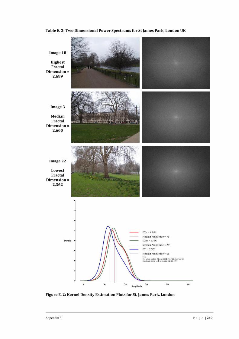
Appendix E P a g e | 249
Table E. 2: Two Dimensional Power Spectrums for St James Park, London UK
Image 18
HighestFractal
Dimension =2.689
Image 3
MedianFractal
Dimension =2.600
Image 22
LowestFractal
Dimension =2.362
Figure E. 2: Kernel Density Estimation Plots for St. James Park, London

Appendix E P a g e | 250
Table E. 3: Two Dimensional Power Spectrums for Green Park, London UK
Image 3
HighestFractal
Dimension =2.656
Image 10
MedianFractal
Dimension =2.591
Image 16
LowestFractal
Dimension =2.436
Figure E. 3: Kernel Density Estimation Plots for Green Park, London

Appendix E P a g e | 251
Table E. 4: Two Dimensional Power Spectrums for Hervey Bay Botanic Gardens Part B
Image 12
HighestFractal
Dimension =2.636
Image 9
MedianFractal
Dimension =2.579
Image 27
LowestFractal
Dimension =2.456
Figure E. 4: Kernel Density Estimation Plots for Hervey Bay Botanic Gardens - Part B

Appendix E P a g e | 252
Table E. 5: Two Dimensional Power Spectrums for Chermside Hills Reserve
Image 17
HighestFractal
Dimension =2.665
Image 39
MedianFractal
Dimension =2.567
Image 76
LowestFractal
Dimension =2.388
Figure E. 5: Kernel Density Estimation Plots for Chermside Hills, Brisbane

Appendix E P a g e | 253
Table E. 6: Two Dimensional Power Spectrums for Brisbane Botanic Gardens
Image 1
HighestFractal
Dimension =2.609
Image 8
MedianFractal
Dimension =2.567
Image 29
LowestFractal
Dimension =2.414
Figure E. 6: Kernel Density Estimation Plots for Brisbane Botanic Gardens

Appendix E P a g e | 254
Table E. 7: Two Dimensional Power Spectrums for Childers Farm Land
Image 35
HighestFractal
Dimension= 2.637
Image 26
MedianFractal
Dimension= 2.557
Image 13
LowestFractal
Dimension= 2.444
Figure E. 7: Kernel Density Estimation Plots for Childers Farm Land

Appendix E P a g e | 255
Table E. 8: Two Dimensional Power Spectrums for Hervey Bay Botanic Gardens Part A
Image 23
HighestFractal
Dimension =2.644
Image 6
MedianFractal
Dimension =2.540
Image 7
LowestFractal
Dimension =2.350
Figure E. 8: Kernel Density Estimation Plots for Hervey Bay Botanic Gardens - Part A

Appendix E P a g e | 256
Table E. 9: Two Dimensional Power Spectrums for Brisbane City Botanic Gardens
Image 13
HighestFractal
Dimension =2.591
Image31
MedianFractal
Dimension =2.514
Image 18
LowestFractal
Dimension =2.307
Figure E. 9: Kernel Density Estimation Plots for Brisbane City Botanic Gardens

Appendix E P a g e | 257
Table E. 10: Two Dimensional Power Spectrums for Roma Street Parklands, Brisbane
Image 32
HighestFractal
Dimension =2.621
Image 7
MedianFractal
Dimension =2.505
Image 28
LowestFractal
Dimension =2.134
Figure E. 10: Kernel Density Estimation Plots for Roma Street Parklands, Brisbane

Appendix E P a g e | 258
Table E. 11: Two Dimensional Power Spectrums for London East Central
Image 4
HighestFractal
Dimension =2.632
Image 28
MedianFractal
Dimension =2.491
Image 61
LowestFractal
Dimension =2.397
Figure E. 11: Kernel Density Estimation Plots for London East Central

Appendix E P a g e | 259
Table E. 12: Two Dimensional Power Spectrums for Dundowran Beach
Image 48
HighestFractal
Dimension =2.745
Image 43
MedianFractal
Dimension =2.489
Image 50
LowestFractal
Dimension =2.384
Figure E. 12: Kernel Density Estimation Plots for Dundowran Beach, Hervey Bay

Appendix E P a g e | 260
Table E. 13: Two Dimensional Power Spectrums for South Bank Parklands
Image 12
HighestFractal
Dimension =2.608
Image 94
MedianFractal
Dimension =2.487
Image 20
LowestFractal
Dimension =2.207
Figure E. 13: Kernel Density Estimation Plots for South Bank Parklands, Brisbane
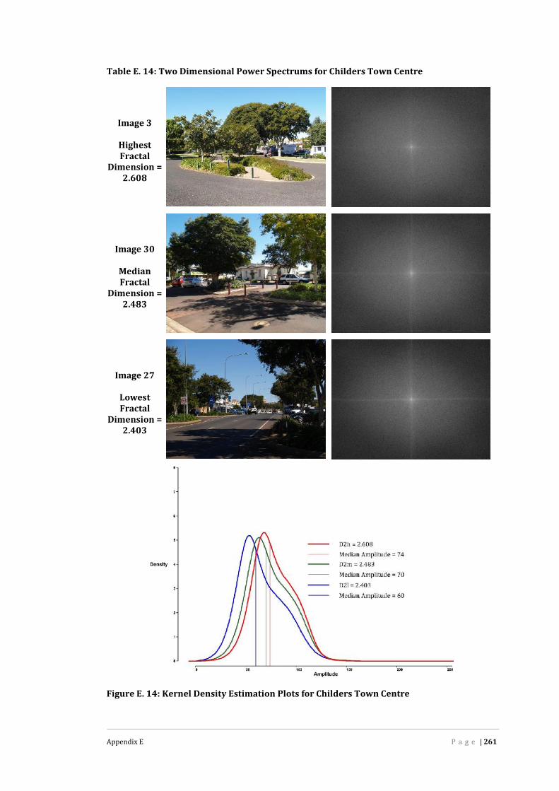
Appendix E P a g e | 261
Table E. 14: Two Dimensional Power Spectrums for Childers Town Centre
Image 3
HighestFractal
Dimension =2.608
Image 30
MedianFractal
Dimension =2.483
Image 27
LowestFractal
Dimension =2.403
Figure E. 14: Kernel Density Estimation Plots for Childers Town Centre

Appendix E P a g e | 262
Table E. 15: Two Dimensional Power Spectrums for Hervey Bay Esplanade
Image 2
HighestFractal
Dimension =2.583
Image 27
MedianFractal
Dimension =2.476
Image 50
LowestFractal
Dimension =2.323
Figure E. 15: Kernel Density Estimation Plots for Hervey Bay Esplanade

Appendix E P a g e | 263
Table E. 16: Two Dimensional Power Spectrums for Cranbourne Botanic Gardens
Image 49
HighestFractal
Dimension =2.640
Image 3
MedianFractal
Dimension =2.468
Image 13
LowestFractal
Dimension =2.198
Figure E. 16: Kernel Density Estimation Plots for Cranbourne Botanic Gardens, Victoria

Appendix E P a g e | 264
Table E. 17: Two Dimensional Power Spectrums for Toowoomba City Centre
Image 7
HighestFractal
Dimension =2.558
Image 37
MedianFractal
Dimension =2.458
Image 45
LowestFractal
Dimension =2.356
Figure E. 17: Kernel Density Estimation Plots for Toowoomba City Centre
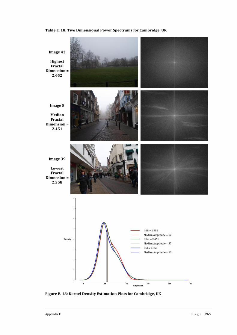
Appendix E P a g e | 265
Table E. 18: Two Dimensional Power Spectrums for Cambridge, UK
Image 43
HighestFractal
Dimension =2.652
Image 8
MedianFractal
Dimension =2.451
Image 39
LowestFractal
Dimension =2.358
Figure E. 18: Kernel Density Estimation Plots for Cambridge, UK
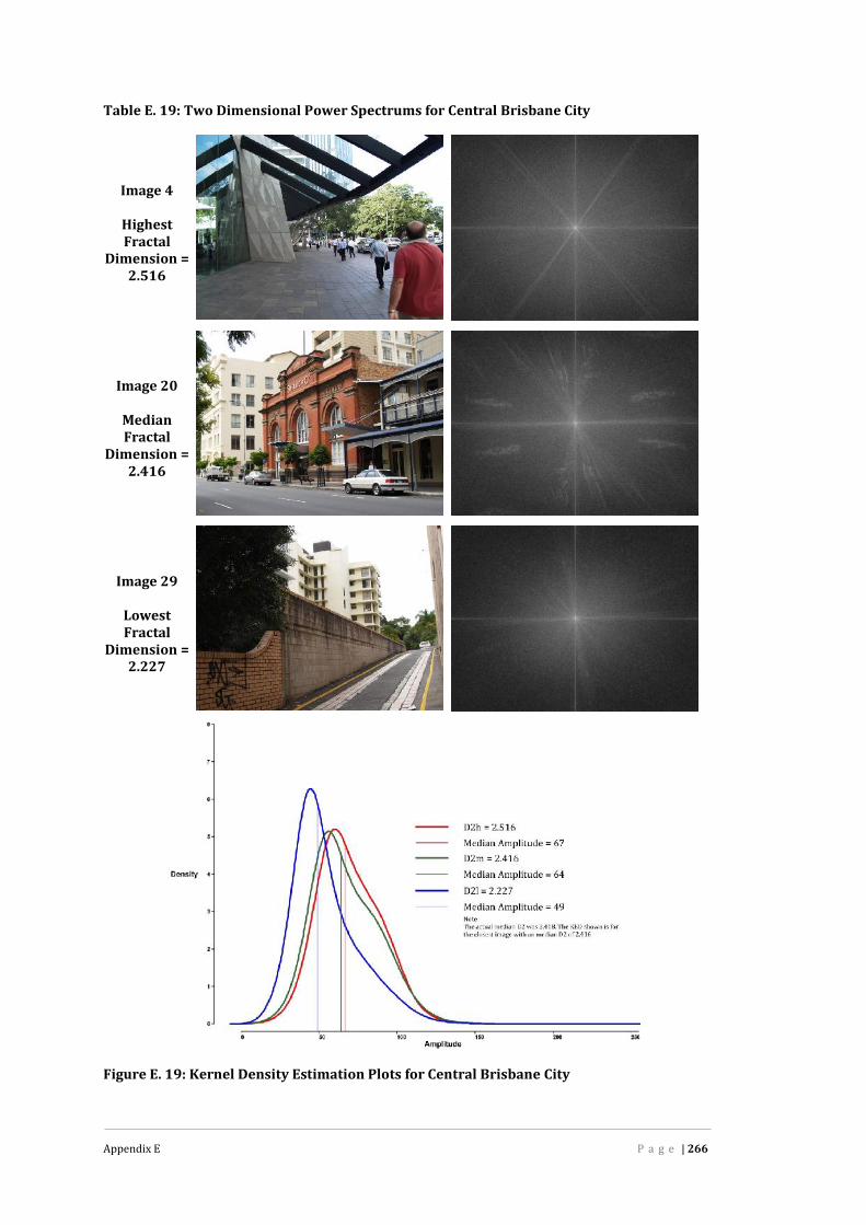
Appendix E P a g e | 266
Table E. 19: Two Dimensional Power Spectrums for Central Brisbane City
Image 4
HighestFractal
Dimension =2.516
Image 20
MedianFractal
Dimension =2.416
Image 29
LowestFractal
Dimension =2.227
Figure E. 19: Kernel Density Estimation Plots for Central Brisbane City

Appendix E P a g e | 267
Table E. 20: Two Dimensional Power Spectrums for London West One
Image 85
HighestFractal
Dimension =2.627
Image 1
MedianFractal
Dimension =2.415
Image 37
LowestFractal
Dimension =2.158
Figure E. 200: Kernel Density Estimation Plots for London West One

Appendix E P a g e | 268
Table E. 21: Two Dimensional Power Spectrums for Melbourne Docklands
Image 3
HighestFractal
Dimension =2.548
Image 38
MedianFractal
Dimension =2.417
Image 8
LowestFractal
Dimension =2.305
Figure E. 211: Kernel Density Estimation Plots for Melbourne Docklands

Appendix E P a g e | 269
Section 2: Standard Histogram Components
Figure E. 22: Histogram Components

References P a g e | 270
References
A.I.L.A. Adapting to Climate Change: Green Infrastructure. (2011).http://www.aila.org.au/greeninfrastructure/Adams, J. M. Global Land Environments Since the Last Interglacial. (1997). Oak RidgeNational Laboratory, TN, USA. http://www.esd.ornl.gov/ern/qen/nerc.htmlAILA (2009). The Australian Landscape Charter. Australian Institute of LandscapeArchitectsAlexander, C. (2002). The Nature of Order: An Essay on the Art of Building and the Natureof the Universe, Berkeley, California: The Centre for Environmental Structure,PageANON (1970). Romanticism in the Visual Arts. In: Osborne, H. (ed.) The OxfordCompanion to Art. New York: Oxford University PressAppleton, J. (1996). The Experience of Landscape, Chichester: John Wiley & Sons, PageArnheim, R. (1974). Art and Visual Perception: A Psychology of the Creative Eye,Berkeley: University of California Press, Pageartisan SUPERNATURE: Pioneering Design Inspired by Nature. (2009). Brisbane.http://www.liveqlddesignworld.com/Audi, R. (ed.) (1999). The Cambridge Dictionary of Philosophy, Cambridge: CambridgeUniversity PressAvnir, D., Biham, O., Lidar, D. & Malcai, O. (1998). Is the Geometry of Nature Fractal?Science, 279, 39-40Baird, C. T. (2002). Sacred Ground: Must Sustainable Landscapes Mimic the Form andSpatial Organisation of Nature? In: CELA 2002: GroundWork, The Faculty ofLandscape Architecture, SUNY College of Environmental Science and Forestry,Syracuse, New York. Council of Educators in Landscape Architecture, 9-15Barry, J. (1994). The Limits of the Shallow and the Deep: Green Politics, Philosophy, andPraxis. Environmental Politics, 3, 369-394Batey, M. (2001). Shaftesbury, Anthony Ashley Cooper. In: Jellicoe, G., Jellicoe, S., Goode,P. & Lancaster, M. (eds.) The Oxford Companion to Gardens. Oxford: OxfordUniversity PressBatty, M. & Longley, P. (1994). Fractal Cities: A Geometry of Form and Function, London:Academic Press Limited, PageBenguigui, L. (2000). When and Where is a City Fractal? Environment and Planning B:Planning and Design, 27, 507-519Bennett, K. (2010). The Chaos Theory of Evolution. New Scientist, 208, 28-31

References P a g e | 271
Bentley, I., Alcock, A., Murrain, P., McGlynn, S. & Smith, G. (1985). ResponsiveEnvironments: A Manual for Designers, London: The Architectural Press, PageBerg, A. E. v. d. (2007). Preference for Nature in Urbanized Societies: Stress,Restoration, and the Pursuit of Sustainability. Journal of Social Issues, 63, 79-96Berleant, A. (1992). The Aesthetics of Environment, Philadelphia: Temple UniversityPress, PageBerlin, J. (2010) The Big Idea: Gaudi's Masterpiece National Geographic 22-27Berofsky, B. (1999). Determinism. In: Audi, R. (ed.) The Cambridge Dictionary ofPhilosophy. Second ed. Cambridge: Cambridge University PressBillock, V. A. (2000). Neural Acclimation to 1/f Spatial Frequency Spectra in NaturalImages Transduced by the Human Visual System. Physica D, 137, 379-391Bourassa, S. (1991). The Aesthetics of Landscape, London: Belhaven Press, PageBovill, C. (1996). Fractal Geometry in Architecture and Design, Boston: Birkhauser, PageBrady, E. (1998). Imagination and the Aesthetic Appreciation of Nature. The Journal ofAesthetics and Art Criticism, 56, 139-147Brady, E. (2003). Aesthetics of the Natural Environment, Tuscaloosa: University ofAlabama Press, PageBriggs, J. (1991). Reflectaphors: The (implicate) Universe as a Work of Art. In: Hiley, B.& Peat, F. D. (eds.) Quantum Implications: Essays in Honour of David Bohm.London: RoutledgeBriggs, J. (1992). Fractals: The Patterns of Chaos, London: Thames and Hudson, PageBull, C. (1996). A Purposeful Aesthetic? Valuing Landscape Style and Meaning in theEcological Age. Landscape Australia, 18, 24-30Burke, E. (1990). A Philosophical Enquiry into the Origin of our Ideas of the Sublimeand Beautiful. In: Phillips, A. (ed.) Edmund Burke: A Philosophical Enquiry.Second ed. Oxford: Oxford University PressBurnham, D. Kant's Aesthetics. (2005).Butchvarov, P. (1999a). Metaphysical Realism. In: Audi, R. (ed.) The CambridgeDictionary of Philosophy. Second ed. Cambridge: Cambridge University PressButchvarov, P. (1999b). Metaphysics. In: Audi, R. (ed.) The Cambridge Dictionary ofPhilosophy. Second ed. Cambridge: Cambridge University PressCarlson, A. (1981). Nature, Aesthetics, Judgement, and Objectivity. The Journal ofAesthetics and Art Criticism, 40, 15-27Carlson, A. (2001). Environmental Aesthetics. In: Gaut, B. & Lopes, D. M. (eds.) TheRoutledge Companion to Aesthetics. London: RoutledgeCarlson, A. (2002). Aesthetics and the Environment, New York: Routledge, Page

References P a g e | 272
Carroll, N., Moore, M. & Seeley, W. P. (2011). The Philosophy of Art and Aesthetics,Psychology, and Neuroscicnce: Studies in Literature, Visual Arts, and Music. In:Shimamura, A. P. & Palmer, S. E. (eds.) Aesthetic Science: Connecting Minds,Brains, and Experience. New York: Oxford University PressCarson, R. (1962). Silent Spring: Houghton Miffin, PageChen, Y. & Zhou, Y. (2008). Scaling laws and indications of self-organized criticality inurban systems. Chaos, Solitons & Fractals, 35, 85-98Chow, M. (2007). Quantum Theory Cannot Hurt You, London: Faber and Faber Limited,PageConnor, S. Fourty Years since the first pictures of earth from space. (2009). TheIndependent: Science. http://www.independent.co.uk/news/science/forty-years-since-the-first-picture-of-earth-from-space-1297569.htmlCooper, J. & Oskrochi, R. (2008). Fractal analysis of street vistas: a potential tool forassessing levels of visual variety in everyday street scenes. Environment andPlanning B: Planning and Design, 35, 349-363Cooper, J., Watkinson, D. & Oskrochi, R. (2010). Fractal analysis and perception of visualquality in everyday street vistas. Environment and Planning B: Planning andDesign, 37, 808-822Cormac, E. M. & Stamenov, M. I. (1996). Introduction. In: Cormac, E. R. M. & Stamenov,M. I. (eds.) Fractals of Brain, Fractals of Mind: In Search of a Symmetry Bond.Amsterdam: John Benjamins Publishing CoCorner, J. (1991). A Discourse on Theory II: Three Tyrannies of Contemporary Theoryand the Alternative of Hermeneutics. Landscape Journal, 10, 115-133Corner, J. (1997). Ecology and Landscape as Agents of Creativity. In: Thompson, G. F. &Steiner, F. R. (eds.) Ecological Design and Planning. New York: John Wiley &Sons, IncCorner, J. (1999). Recovering Landscape as a Critical Cultural Practice. In: Corner, J.(ed.) Recovering Landscape: Essays in Contemporary Landscape Architecture.New York: Princeton Architectural PressCosgrove, D. E. (1998). Social Formation and Symbolic Landscape, Madison, Wisconsin:The University of Wisconsin Press, PageCosgrove, D. E. (2003). Landscape: Ecology and Semiosis. In: Palang, H. & Fry, G. (eds.)Landscape Interfaces: Cultural Heritage in Changing Landscapes. Dordrecht:Kluwer Academic PublishersCostonis, J. j. (1982). Law and aesthetics: A Critique and a Reformulation of the Dilemas.Michigan Law Review, 80, 355-461Cotgreave, P. & Forseth, I. (2002). Introductory Ecology. Oxford: Blackwell Science Ltd

References P a g e | 273
Cottingham, J. (1999). Descartes, René. In: Audi, R. (ed.) The Cambridge Dictionary ofPhilosophy. Second ed. Cambridge: Cambridge University PressCottingham, J. (2001). Descartes: Descartes' Philosophy of Mind. In: Monk, R. & Raphael,F. (eds.) The Great Philosophers. London: PhoenixCowan, G. A. (1976). A Natural Fission Reactor. Scientfic America, 235, 36Crawford, D. W. (2001). Kant. In: Gaut, B. & Lopes, D. M. (eds.) The Routledge Companionto Aesthetics. London: RoutledgeCrewe, K. & Forsyth, A. (2003). LandSCAPES: A Typology of Approaches to LandscapeArchitecture. Landscape Journal, 22, 37-53Crilly, T. (2007). 50 Mathematical Ideas You Really Need to Know, London: Quercus,PageCrompton, A. (2001). The Fractal Nature of Everyday Environments. Environment andPlanning B: Planning and Design, 28, 243-254Crompton, A. (2002). Fractals and Picturesque Composition. Environment and PlanningB: Planning and Design, 29, 451-459Dennis, S. F. (2002). The Landscape Literacy trap, or A Guide to LandscapeInterpretation in a Postmodern World. In: Deming, M. E., ed. CELA 2002:GroundWork, The Faculty of Landscape Architecture, SUNY College ofEnvironmental Science and Forestry, Syracuse, New York. Council of Educatorsin Landscape Architecture, 25-31Desmond, R. (2001). Pope Alexander (1688-1744)). In: Jellicoe, G., Jellicoe, S., Goode, P.& Lancaster, M. (eds.) The Oxford Companion to Gardens. Oxford: OxfordUniversity PressDewey, J. (1980). Art as Experience, New York: PerigeeBooks, PageDoug, T. An Introduction to the Kernel Density Estimation. (2001). University of WesternAustralia. http://school.maths.uwa.edu.au/~duongt/seminars/intro2kde/Dretske, F. (1999). Perception. In: Audi, R. (ed.) The Cambridge Dictionary of Philosophy.Second ed. Cambridge: Cambridge University PressDunnett, N. (2004). The Dynamic Nature of Plant Communities - Pattern and Process inDesigned Plant Communities. In: Dunnett, N. & Hitchmough, J. (eds.) TheDynamic Landscape. London: Spon PressEagleton, T. (1996). The illusions of postmodernism, Oxford, UK: Balckwell PublishersLimited, PageEaton, M. M. (1992). Where's the Spear?The Question of Aesthetic Relevance. BritishJournal of Aesthetics, 32, 1-12Eaton, M. M. (1997). The Beauty That Requires Health. In: Nassauer, J. I. (ed.) PlacingNature: Culture and Landscape Ecology. Washington, DC: Island Press
References P a g e | 274
Eaton, M. M. (1998). Fact and Fiction in the Aesthetic Appreciation of Nature. TheJournal of Aesthetics and Art Criticism, 56, 149-156Emerson, R. W. (1991 [1836]). Nature. In: Elder, J. (ed.) Nature Walking. Boston:Beacon PressEvernden, N. (1992). The Social Creation of Nature, Baltimore: The Johns HopkinsUniversity Press, PageField, D. J. (1987). Relations Between the Statistics of Natural Images and the ResponseProperties of Cortical Cells. Journal of the Optical Society of America, 4, 2379-2393Fisher, R., Perkins, S., Walker, A. & Wolfart, E. Fourier Transform. (2003).http://homepages.inf.ed.ac.uk/rbf/HIPR2/fourier.htmFlaherty, E. (2010). Fractals, Religion and Landscape Architecture. LandscapeArchitecture Electronic Forum. 19 March 2010 ed.: Syracuse UniversityFrankhauser, P. (2008). Fractal Geometry for Measuring and Modelling Urban Patterns.In: Albeverio, S., Andrey, D., Giordano, P. & Vancheri, A. (eds.) The Dynamics ofComplex Urban Systems. Physica-Verlag HDFung, S. & Jackson, M. (1996). Dualism and Polarsim: Structures of Architectural andLandscape Archtectural Discourse in China and the West. Interstices 4,Galinsky, A. & Whitson, J. (2008). Lacking Control Increases Illusory Pattern Perception.Science, 322, 115Garrett, D. (1999). Spinoza, Baruch. In: Audi, R. (ed.) The Cambridge Dictionary ofPhilosophy. Second ed. Cambridge: Cambridge University PressGill, M. B. Lord Shaftesbury [Anthony Ashley Cooper, 3rd Earl of Shaftesbury]. (2006).Stanford. http://plato.stanford.edu/archives/fall2008/entries/shaftesbury/
Out of the Ashes, 2011. Directed by Gilmour, D. Australia: ABCGilpin, W. (1808). Three Essays: on Picturesque Beauty on Picturesque Travel and onSketching Landscape., London: Cadell and Davis, PageGleick, J. (1998). Chaos: Making a New Science, London: Vintage, PageGodlovitch, S. (1998). Evaluating Nature Aesthetically. The Journal of Aesthetics and ArtCriticism, 56, 113-125Graham, D. W. Heraclitus (fl. c.500 BCE). (2011). http://www.iep.utm.edu/heraclit/Green, R. (2006). Global environmental change and the poetry of place: thoughts on theeducation of landscape architects. Landscape Review, 6, 11-24Groat, L. & Wang, D. (2002). Architectural Research Methods, New York: John Wiley &Sons, Inc, PageGuyer, P. 18th Century German Aesthetics. (2007).http://plato.stanford.edu/archives/fall2008/entries/aesthetics-18th-german/
References P a g e | 275
Hagerhall, C. M., Purcell, T. & Taylor, R. (2004). Fractal Dimension of LandscapeSilhouette Outlines as a Predictor of Landscape Preference. Journal ofEnvironmental Psychology, 24, 247-255Harker, D., Libby, G., Harker, K., Evans, S. & Evans, M. (1999). Landscape RestorationHandbook, Boca Raton, USA: Lewis Publishers, PageHartmann, P. & Apaolaza-Ibanez, N. (2009). Beyond Savanna: An evolutionary andenvironmental psychology appraoch to behavioural effects of nature scenery ingreen advertising. Journal of Environmental Psychology, 1-10Hay, P. (2002). Main Currents in Western Environmental Thought, Sydney: University ofNew South Wales Press Ltd, PageHendry, G. S. (1980). Theology of Nature, Philadelphia: The Westminster Press, PageHepburn, R. (1966). Contemporary Aesthetics and the Neglect of Natural Beauty. In:Williams, B. & Montefiore, A. (eds.) British Analytical Philosophy. RoutledgeHill, D. & Daniel, T. C. (2008). Foundations for an Ecological Aesthetic: Can InformationAlter Landscape Preference. Society and Natural Resources, 21, 34-49Hogarth, W. (1753). The Analysis of Beauty. In: Burke, J. (ed.) William Hogarth: TheAnalysis of Beauty. Oxford: Clarendon Press, 1955Howett, C. (1987). Systems, Signs, Sensibilities: Sources for a New Landscape Aesthetic.Landscape Journal, 6, 1-12Hunt, J. D. (1991). The Garden as Cultural Object. In: Wrede, S. & Adams, W. H. (eds.)Denatured Visions: Landscape and Culture in the Twentieth Century. New York:The Museum of Modern Art, New YorkHunt, J. D. (2002). The Picturesque Garden in Europe, London: Thames & Hudson, PageHunt, J. D. & Willis, P. (eds.) (1988). The Genius of the Place: The English LandscapeGarden 1620--1820, Cambridge, Massachusetts: The MIT PressHunt, J. D. & Willlis, P. (1988). Alexander Pope (1688--1744). The Genius of the Place: TheEnglish Landscape Garden 1620 - 1820. Cambridge, Massachusetts: The MITPressInwood, M. (2001). Hegel. In: Gaut, B. & Lopes, D. M. (eds.) The Routledge Companion toAesthetics. London: RoutledgeJackson, J. B. (1984). Discovering the Vernacular Landscape, New Haven: Yale UniversityPress, PageJencks, C. A. (2003). The Garden of Cosmic Specultation, London: Frances Lincoln Ltd,PageJennings, T. (2010). Ecology. Saddleback Educational Publishing

References P a g e | 276
Jurgens, H., Peitgen, H. O. & Saupe, D. (1990). The Language of Fractals. ScientificAmerica, 263, 40-47Kant, I. (2008 [1783]). Prolegomena to Any Future Metaphysics: Forgotten Books, PageKant, I. (2008 [1790]). Critique of Judgement: Forgotten Books, PageKaplan, R. & Kaplan, S. (1989). The Experience of Nature: A Psychological Perspective,Cambridge: Cambridge University Press, PageKaplan, R., Kaplan, S. & Ryan, R. L. (1998). With People in Mind: Design and Managementof Everyday Nature, Washington D.C.: Island Press, PageKaplan, S. (1982). Cognition and Environment: Functioning in an Uncertain World, NewYork: Praeger, PageKaram, A. The Natural Nuclear Reactor at Oklo: A Comparison with Modern NuclearReactors. (2005). Idaho State University.http://www.physics.isu.edu/radinf/Files/Okloreactor.pdfKemal, S. (1997). Kant's Aesthetic Theory, London: Macmillan Press Ltd, PageKemmer, S. Chronology of Human Evolution. (2008). RICE University.http://www.ruf.rice.edu/~kemmer/Evol/timeline.htmlKemp, E. (1850). How to Lay Out a Small Garden, London: Bradbury and Evans, PageKenkel, N. C. & Walker, D. J. (1996). Fractals in the Biological Sciences. COENOSES, 11,77-100Knill, D. C., Field, D. & Kersten, D. (1990). Human Discrimination of Fractal Images.Journal of the Optical Society of America, 7, 1113-1123Koh, J. (1988). An Ecological Aesthetic. Landscape Journal, 7, 177-191Kolenda, K. (1999). Humanism. In: Audi, R. (ed.) The Cambridge Dictionary ofPhilosophy. Second ed. Cambridge: Cambridge University PressLamb, R. & Purcell, A. (1990). Perception of naturalness in landscape and itsrelationship to vegetation structure. Landscape and Urban Planning, 19, 333-352Landplan (2007). Hervey Bay Botanic Gardens: Master Plan Review. Draft Report #2.Landplan Landscape ArchitectsLane, D., Lu, J., Peres, C. & Zitec, E. Online Statsitics: An Interactive Multimedia Course ofStudy. (2011). http://onlinestatbook.com/chapter10/pairwise.htmlLee, A. B., Mumford, D. & Huang, J. (2001). Occlusion Models for Natural Images: AStatistical Study of a Scale-Invariant Dead Leaves Model. International Journal ofComputer Vision, 41, 35-59Leopold, A. (1989). A Sand Country Almanac And Sketches Here and There, Oxford:Oxford University Press, Page
References P a g e | 277
Li, B.-L. (2000). Fractal Geometry Applications in Description and Analysis of PatchPatterns and Patch Dynamics. Ecological Modeling, 132, 33-50Livio, M. (2002). The Golden Ratio: The Story of Phi, the Extra Ordinary Number ofNature, Art and Beauty, London: Headline Book Publishing, PageLomborg, B. (2008). Cool It, New York: Vintage Books, PageLorenz, W. E. (2002). Fractals and Fractal Architecture. Master, Vienna University ofTechnologyLorenz, W. E. (2009). Fractal Geometry of Architecture. 27th eCAADe CONFERENCE;Computation: The new Realm of Architectural Design, (2009). Istanbul, Turkey:Loudon, J. C. (1804). Observations on the Formation and Management of Useful andOrnamental Plantations on the Theory and Practice of Landscape Gardening,Edinburgh: Archibald Constable & Co, PageLoudon, J. C. (1838). The Suburban Gardener and Villa Companion, London: GarlandPublishing Inc, PageLovelock, J. (1979). Gaia: A New Look at Life on Earth, Oxford: Oxford University Press,PageMagnus, B. (1999). Postmodern. In: Audi, R. (ed.) The Cambridge Dictionary ofPhilosophy. Second ed. Cambridge: Cambridge University PressMandelbrot, B. B. (1983). The Fractal Geometry of Nature, New York: W H Freeman andCompany, PageMarsh, G. P. (1869). Man and Nature, New York: Charles Scribner & Co, PageMcDonough, W. (2004) Natural Designs New Scientist 2439 46-48McHarg, I. (1969). Design with Nature, New York: Natural History Press, PageMcIvor, J. G. & McIntyre, S. (2002). Understanding Grassy Woodland Ecosystems. In:McIntyre, S., McIvor, J. G. & Heard, K. M. (eds.) Managing and Conserving GrassyWoodlands. Melbourne: CSIRO PublishingMclaughlin, B. P. (1999). Philosophy of Mind. In: Audi, R. (ed.) The Cambridge Dictionaryof Philosophy. Second ed. Cambridge: Cambridge University PressMerchant, C. (1982). The Death of Nature: Women, Ecology and the Scientific Revolution,London: Wildwood House Ltd, PageMeyer, E. K. (2008). Sustaining Beauty. The performance of apperance. Journal ofLandscape Architecture, 6-23Mozingo, L. A. (1997). The Aesthetics of Ecological Design: Seeing Science as Culture.Landscape Journal, 16, 46-59Muir, J. (1890). Features of the Proposed Yosemite National Park. The CenturyMagazine, 40, 656-667

References P a g e | 278
Musacchio, L. R. (2009). The scientific basis for the design of landscape sustainability: Aconceptual framework for translational landscape research and practice ofdesigned landscapes and the six Es of landscape sustainability. LandscapeEcology, 24, 993-1013Nassauer, J. I. (1992). The Appearance of Ecological Systems as a Matter of Policy.Landscape Ecology, 6, 239-250Nassauer, J. I. (1997a). Cultural Sustainability: Aligning Aesthetics and Ecology. In:Nassauer, J. I. (ed.) Placing Nature: Culture and Landscape Ecology. WashingtonD.C.: Island PressNassauer, J. I. (ed.) (1997b). Placing Nature: Culture and Landscape Ecology,Washington D.C.: Island PressNassauer, J. I. (2002). Messy Ecosystems, Orderly Frames. In: Swaffield, S. (ed.) Theoryin Landscape Architecture: A Reader. Philadelphia: University of PennsylvaniaPressNassauer, J. I. & Opdam, P. (2008). Design in Science: extending the landscape ecologyparadigm. Landscape Ecology, 23, 633-644Nohl, W. (2001). Sustainable landscape use and aesthetic perception-preliminaryreflections on future landscape aesthetics. Landscape and Urban Planning, 54,223-237O'Donnell, K. (2003). Postmodernism, Oxford: Lion Publishing plc, PageO'Neil, D. Language and Culture: An Introduction to Human Communication. (2006). SanMarcos, California: Palomar College.http://anthro.palomar.edu/language/Default.htmOlwig, K. R. (1996). Recovering the Substantive Nature of Landscape. Annals of theAssociation of American Geographers 86, 630-653Ostwald, M. J., Vaughan, J. & Tucker, C. (2008). Characterstic Visual Complexity: FractalDimensions in the Architecture of Frank Lloyd Wright and Le Corbusier. In:Williams, K. (ed.) Nexus VII: Architecture and Mathematics. Turin: Kim WilliamsBooksPalka, E. J. (1995). Coming to Grips with the Concept of Landscape. Landscape Journal,14, 63-73Pan, F., Chen, J. & Huang, J. (2009). Discriminating between photorealistic computergraphics and natural images using fractal geometry. Science in China Series F:Information Sciences, 52, 329-337Papanek, V. (1995). The Green Imperative: Ecology and Ethics in Design and Architecture,London: Thames and Hudson, PagePentland, A. P. (1984). Fractal-Based Description of Natural Scenes. IEEE Transactionon Pattern Analysis and Machine Intelligence, PAMI-6, 661674

References P a g e | 279
Phillips, C. (2003). Sustainable Place, Chichester, England: John Wiley & Sons Ltd, PagePrice, U. (1796). An Essay on the Picturesque as Compared with the Sublime and theBeautiful; and on the Use of Studying Pictures for the Purpose of Improving RealLandscape, London: J Robinson, PagePurcell, T., Peron, E. & Berto, R. (2001). Why do Preferences Differ Between SceneTypes? Environment and Behaviour, 33, 93-106Quest-Ritson, C. (2001). The English Garden: A Social History, London: Penguin Books,PageQuincy, A.-C. Q. d. (1837). An Essay on the Nature, the End, and the Means of theImitation in the Fine Arts, London: Smith, Elder & Co., PageReeves, R. 24 August 2006 (2006). RE: Notes on Statistics. Type to Perry, S.Reeves, R. 16 April 2007 (2007). RE: Fractal Dimension of Images. Type to Perry, S.Reeves, R. 24 February 2009 (2009). RE: Fourier Power Spectrum. Type to Perry, S.Relph, E. (1986). Place and Placelessness, London: Pion Limited, PageRichards, R. (2001). A New Aesthetic for Environmental Awareness: Chaos Theory, theBeauty of Nature, and our Broader Humanistiv Identity. Journal of HumanisticPsychology, 41, 59--95Richards, R. (ed.) (2007a). Everyday Creativity and New Views on Human Nature,Washington, DC: American Psychological AssociationRichards, R. (2007b). Everyday Creativity and the Arts. World Futures, 63, 500-525Richardson, T. Tim Richardson Revisits the Garden of Cosmic Speculation. (2007).thinkinggardens.co.uk. http://thinkingardens.co.uk/reviews/tim-richardson-revisits-the-garden-of-cosmic-speculation/Roberts, S., Aguilar, R., Warrenchuk, J., Hudson, C. & Hirshfield, M. Deep Sea Life: On theEdge of the Abyss. (2005). Oceana. http://na.oceana.org/en/news-media/publications/reports/deep-sea-life-on-the-edge-of-the-abyssRobinson, D. Mass Extinction & Divesification. (2006). Harvard University.http://outreach.mcb.harvard.edu/materials.htmRobinson, D. & Groves, J. (1998). Introducing Philosophy, Cambridge: Icon BooksLimited, PageRobinson, D. & Groves, J. (2000). Introducing Plato, London: Icon Books Ltd, PageRogers, E. B. (2001). Landscape Design: A Cultural and Architectural History, New York:Harry N. Abrams, Inc., PageRuderman, D. L. (1994). The Statistics of Natural Images. Network: Computation inNeural systems, 5, 517-548

References P a g e | 280
Ruderman, D. L. (1997). Origins of Scaling in Natural Images. Vision Research, 37, 3385-3398Ruderman, D. L. & Bialek, W. (1994). Statistics of Natural Images: Scaling in the Woods.Physical Review Letters, 73, 814-817Ruskin, J. (1904). The Works of John Ruskin. In: Cook, E. & Wedderburn, A. (eds.).London: George AllenRuss, J. C. (2007). The Image Processing Handbook, Boca Raton, FL: Taylor & Francisgroup, PageRussell, B. (1959). The Problems of Philosophy, London: Oxford University Press, PageSala, N. (2001). The Presense of the Self-Similarity in Architecture: Some Examples. In:Novak, M. M. (ed.) Emergent Nature: Patterns, Growth and Scaling the Sciences.London: World Scientific Publishing Co.Scruton, R. (2001). Spinoza. In: Monk, R. & Raphael, F. (eds.) The Great Philosophers.London: PhoenixShelley, J. The Concept of Aesthetics. (2009a). Stanford.http://plato.stanford.edu/archives/fall2009/entries/aesthetic-conceptShelley, J. The Concept of Aesthetics. (2009b). Stanford: The Stanford Encyclopedia ofPhilosophy. http://plato.stanford.edu/archives/fall2009/entries/aesthetic-conceptShelley, J. 18th Century British Aesthetics. (2010).http://plato.stanford.edu/archives/fall2010/entries/aesthetics-18th-british/Sim, J. (2001). Landscape Design Theory Primer. Brisbane: Queensland University ofTechnologySim, J. C. R. (1999). Designed Landscapes in Queensland, 1859-1939: Experimentation -Adaptation - Innovation. PhD, Queensland University of TechnologySimo, M. L. (1988). Loudon and the Landscape: From Country Seat to Metropolis 1783-1843, New Haven: Yale University Press, PageSimonds, J. O. (1983). Landscape Architecture: A Manual of Site Planning and Design,New York: McGraw-Hill, PageSorvig, K. (2002). Nature / Culture / Words / Landscapes. Landscape Journal, 21, 1-14Spehar, B., Clifford, C. W. G., Newell, B. R. & Taylor, R. (2003). Universal Aesthetics ofFractals. Computers & Graphics, 27, 813-820Spirn, A. W. (1947). The Granite Garden: Urban Nature and Human design, Philiadelphia:Basic Books, PageSpirn, A. W. (1988). The Poetics of City and Nature: Towards a New Aesthetic for UrbanDesign. Landscape Journal, 7, 108-126
References P a g e | 281
Spirn, A. W. (1996). Constructing Nature: The Legacy of Frederick Law Olmsted. In:Cronon, W. (ed.) Uncommon Ground: Towards Reinventing Nature. New York: WN NortonStroud, D. (2001). Kent William (1685-1748). In: Jellicoe, G., Jellicoe, S., Goode, P. &Lancaster, M. (eds.) The Oxford Companion to Gardens. Oxford: OxfordUniversity PressSutton, M. Q. & Anderson, E. N. (2010). Introduction to Cultural Ecology, Plymouth:Alltamira Press, PageSutton, R. (2010). Re: Larch Digest - 23 March 2010 to 24 March 2010. LandscapeArchitecture Electronic Forum. 25 March 2010 ed.: Syracuse UniversitySuzuki, D. (1997). The Sacred Balance: Rediscovering Our Place in Nature, St, Leonards,NSW: Allen & Unwin, PageSwaffield, S. (2002). Theory in Landscape Architecture: Introduction. In: Swaffield, S.(ed.) Theory in Landscape Architecture: A Reader. Philadelphia: University ofPennsylvania PressSymes, M. (2001). Regents Park. In: Jellicoe, G., Jellicoe, S., Goode, P. & Lancaster, M.(eds.) The Oxford Companion to Gardens. Oxford: Oxford University PressTaylor, R. Fractal Expressionism — Where Art Meets Science. (2002). University ofOregon: Materials Science Institute.http://materialscience.uoregon.edu/taylor/art/complexity1.pdfTaylor, R., Spehar, B., Wise, J. A., Clifford, C. W. G., Newell, B. R., Hagerhall, C. M., Purcell,T. & Martin, T. P. Perceptual and Physiological Responses to the Visual Complexityof Pollock’s Dripped Fractal Patterns. (2005). University of Oregon: MaterialsScience Institute. http://materialscience.uoregon.edu/taylor/art/Boston1.pdfTaylor, R. P., Micolich, A. P. & Jones, D. (1999). Fractal Analysis of Pollock's DripPaintings. Nature, 399, 422Thacker, C. (1979). The History of Gardens, London: Croom Helm, PageThayer, R. L. (1976). Visual Ecology: Revitalising the Aesthetic of LandscapeArchitecture. Landscape, 20, 37-43Thayer, R. L. (1989). The Experience of Sustainable Landscapes. Landscape Journal, 8,101-109Thayer, R. L. (1994). Gray World, Green Heart: Technology, Nature, and the SustainableLandscape, New York: John Wiley & Sons Inc, PageThayer, R. L. (2002). Gray World, Green Heart. In: Swaffield, S. (ed.) Theory in LandscapeArchitecture. Philadelphia: University of Pennsylvania PressThomas, I., Tannier, C. & Frankhauser, P. (2009). Is there a link between fractaldimension and residential environment at a regional level? Cybergeo: EuropeanJournal of Geography,
References P a g e | 282
Thomas, K. (1984). Man and the Natural World: Changing Attitudes in England 1500-1800, New York: Penguin Books, PageThompson, G. F. & Steiner, F. R. (eds.) (1997). Ecological Design and Planning, NewYork: John Wiley & Sons, IncThompson, I. (2009). rethinking landscape: a critical reader, Abingdon: Routledge, PageThompson, I. H. (2000). The Ethics of Sustainability. In: Benson, J. F. & Roe, M. H. (eds.)Landscape and Sustainability. London: Spon PressThompson, M. (2003). Philosophy of Religion, London: Hodder headline Ltd, PageThoreau, H. D. (1991). Walking. In: Elder, J. (ed.) Nature Walking. Boston: Beacon PressThwaites, K. (2000). Expressivist Landscape Architecture: the Development of a NewConceptual Framework for Landscape Architecture. Landscape Journal, 19, 201-210Tonder, G. J. V. & Lyons, M. J. (2005). Visual Perception in Japanese Rock Garden Design.Axiomathes, 15, 353-371Townsend, D. (1997). The Picturesque. The Journal of Aesthetics and Art Criticism, 55,365-376Treib, M. (1995). Must Landscape Mean?: Approaches to Significance in RecentLandscape Architecture. Landscape Journal, 14, 47-62Treib, M. (1999). Nature Recalled. In: Corner, J. (ed.) Recovering Landscape: Essays inContemporary Landscape Architecture. New York: Princeton Architectural PressTreib, M. (2002). The Contents of Landscape Form [The Limits of Formalism].Landscape Journal, 20, 119-140Trombley, S. (2001). Objectivity. In: Gaut, B. & Lopes, D. M. (eds.) The RoutledgeCompanion to Aesthetics. London: RoutledgeTrout, J. (1999). Scientific Realism. In: Audi, R. (ed.) The Cambridge Dictionary ofPhilosophy. Second ed. Cambridge: Cambridge University PressTurner, M. J., Blackledge, J. M. & Andrews, P. R. (1998). Fractal Geometry in DigitalImaging, London: Academic Press, PageTurner, T. (2010). Fractals Geometry and the 'imitation of nature'. LandscapeArchitecture Electronic Forum. 22 March 2010 ed.: Syracuse UniversityTurner, T. H. D. (2001a). Gardenesque Style. In: Jellicoe, G., Jellicoe, S., Goode, P. &Lancaster, M. (eds.) The Oxford Companion to Gardens. Oxford: OxfordUniversity PressTurner, T. H. D. (2001b). Loudon, John Charles (1783-1843). In: Jellicoe, G., Jellicoe, S.,Goode, P. & Lancaster, M. (eds.) The Oxford Companion to Gardens. Oxford:Oxford University Press
References P a g e | 283
UCMP The Forest Biome. (2011). University of California Museum of Paleontology.http://www.ucmp.berkeley.edu/exhibits/biomes/forests.phpUlrich, R. S. (1983). Aesthetic and Affective Response to Natural Environments. HumanBehaviour and Environment, 6, 85-125UNESCO Convention on Wetlands of International Importance especially as WaterfowlHabitat. (1971). Ramsar, Iran: UNESCO.http://www.ramsar.org/cda/en/ramsar-documents-texts-convention-on/main/ramsar/1-31-38%5E20671_4000_0__UNWCED (1987). Our Common Future. Stockholm: United Nations World Commissionon Environment and DevelopmentVyzantiadou, M., Avdelas, A. & Zafiropoulos, S. (2007). The application of fractalgeometry to the design of grid or reticulated shell structures. Science Direct:Computer-Aided Design, 39, 51-59Ward, G. (1997). Postmodernism, London: Hodder Headline Limited, PageWatt, S. (1993). A Fractal Geometry of the Mind. HCRL Technical Report 109WCED Our Common Future. (1987). Oslo: United Nations World Commission onEnvironment and Development. http://www.un-documents.net/ocf-cf.htmWhite, L. (1967). The Historical Roots of our Ecological Crisis. Science, 155, 1203-1207Williams, K. (1997). Italian Pavements: Patterns in Space, Singapore: Anchorage Press,PageWilliamson, T. (1995). Polite Landscapes: Gardens and Society in Eighteenth CenturyEngland, Gloucestershire: Sutton Publishing, PageXu, T., Moore, I. D. & Gallant, J. C. (1993). Fractals, Fractal Dimension and Landscapes - AReview. Geomorphology, 8, 245-262