Caitlin Dannhauser  is at  the Villanova School of Business, Villanova University, 800 Lancaster Avenue, Villanova, PA 19085.  She  can be  reached  at  caitlin.dannhauser@villanova.edu. Phone: 610‐519‐4348. Saeid Hoseinzade is at the Sawyer Business School, Suffolk University, 120 Tremont Street, Boston, MA 02108. He can be reached at Email: shoseinzade@suffolk.edu . We thank Pierluigi Balduzzi, Jeffrey Pontiff, Jonathan Reuter, Ronnie Sadka, and Hassan Tehranian for helpful comments. 

The Transformation of Corporate Bond Investors and Fragility:  

Evidence on Mutual Funds and ETFs 

 

Caitlin Dannhauser  

Villanova University 

 

Saeid Hoseinzade  

Suffolk University 

 

 

 

 Investment  vehicles  offering  daily  and  intraday  liquidity  now  have  assets  equivalent  to 

traditional long‐term investors in the corporate bond market. We examine if this transformation 

is a potential source of market fragility. Using an idiosyncratic shock caused by monetary policy, 

we  test  the  impact of unexpected outflows  to various  investment vehicles on  corporate bond 

yields. Relying on within issuer variation, we find that active and index mutual fund outflows 

have no effect on asset prices. However ETF outflows lead to flow‐driven pressure with the yields 

of exposed bonds increasing significantly before reverting seven months later. We attribute the 

differential  effect  to  reduced  cash  buffers  and  to  greater  investment  by  short‐term  positive 

feedback traders in ETFs. Arbitrage is found to be one mechanism by which the risks created by 

these features are propagated to the underlying market. 

 

 

 

 

 

 

 

 

 

 

1  

 

1. Introduction 

Fragility resulting from  the unintended consequences of financial  innovation  is a recurring 

theme in market history (Gennaioli, Shleifer, and Vishny, 2012).1 Following the most recent financial 

crisis, there has been heightened academic and regulatory  interest  in the vulnerabilities created by 

various non‐bank  financial  institutions.  Schmidt, Timmermann,  and Wermers  (2016) observe  that 

pooled vehicles  for which  the  liquidity mismatch becomes magnified during  times of  turmoil are 

especially susceptible to run‐like behavior and its consequences. In the years since, the systemically 

important corporate bond market has seen the assets of nontraditional  investors, open end mutual 

funds and exchange traded funds (ETFs), more than double to nearly match the levels of traditional 

bond investors, insurance companies. Despite providing diversified exposure to the difficult to access 

underlying  market,  the  emergence  of  these  investment  vehicles  has  raised  historically  familiar 

concerns among market participants due to the daily and intraday liquidity they provide relative to 

illiquid corporate bonds, a transformation that is anecdotally referred to as the liquidity illusion. For 

instance,  the 2015 Financial Stability Oversight Council annual  report  lists  the  expansion of  these 

vehicles as a potential emerging  systematic  threat and Bill Gross  expressed  concern  regarding an 

exodus  from ETFs.2 Conversely,  the  Investment Company  Institute argues  that asset managers are 

well aware of their liquidity risks and can manage a buffer to prevent impacting the underlying asset 

prices and major ETF sponsors deem  the  risk created  to be  limited due  to structural  features  that 

mitigate the funds’ interaction with constituent bonds.3,4  

In this paper we provide unique evidence on the asset price implications of flows to corporate 

bond mutual funds and ETFs during a period of turmoil. Although mutual and ETFs are both pooled 

                                                            1 The authors cite collateralized mortgage obligations in the 1980s and 1990s, mortgage backed securities during the 2000s, and money 

market funds in 2008 to motivate the theory that innovations sparked by virtues of diversification, tranching, and insurance offer cash 

flows believed to be good substitutes for the original. Excessive issuance prior to the revelation of news regarding the vulnerability 

of the new securities to unattended risk results in market fragility. 2 “The obvious risk—perhaps better labeled the ‘liquidity illusion’—is that all investors cannot fit through a narrow exit at the same 

time,” Bill Gross. See: https://www.wsj.com/articles/goldman‐sachs‐joins‐bond‐etf‐party‐1496925000  3 ICI 2016 Factbook states “There are many reasons to believe [concerns that outflows to bond funds could pose challenges for fixed‐

income markets]  are  overstated.”  The  reasons  given  are  aggregate  flows  offsetting  the  risk  of  individual  funds,  ETFs  growing 

popularity  in  the  space,  derivatives  usage  to  manage  flows,  and  management  of  a  liquidity  buffer. 

http://www.icifactbook.org/deployedfiles/FactBook/Site%20Properties/pdf/2016_factbook.pdf 4 Bill McNabb, CEO of Vanguard, states “This discovery that most ETF share trading does not lead to any activity in the ETF portfolio 

means  the  impact  of  ETFs  —  and  the  possibility  of  disruption  or  volatility  —  on  the  primary  market  is  limited.”  See: 

https://www.ft.com/content/53054716‐e6e9‐11e6‐893c‐082c54a7f539 

2  

investment vehicles, their distinguishing features make the mechanism through which outflows to the 

funds would  impact  the  pricing  of  the  underlying  distinct.  For  the more  familiar mutual  funds, 

investors can redeem shares for cash at the end of day net asset value (NAV). The consequences of the 

redeeming investor’s outflow are borne by the remaining investors and thus create the potential for 

strategic complementarities. Goldstein, Jiang, and Ng (2015) find that active corporate bond mutual 

funds are particularly susceptible to this behavior and subsequent runs due to a concave flow to return 

relationship rather than the convex relationship found in equity mutual funds (Brown, Harlow, and 

Starks, 1996; Chevalier and Ellison, 1997;  Ippolito, 1992; Lynch and Musto, 2003; Sirri and Tufano, 

1998). The authors  conclude  that  evidence of a major  effect on market prices and potentially  real 

economic activity is needed for these mutual funds to be a major systemic concern.  

ETFs are distinguished from mutual funds by their intraday exchange trading, index focus, 

and in‐kind creation and redemption mechanism that facilitates arbitrage between the ETF shares and 

the  underlying  basket.  These  features  mitigate  concerns  of  runs  induced  by  strategic 

complementarities because  the exiting shareholder bears  the cost of his own actions. Nevertheless, 

recent theoretical works suggests that the absence of these externalities does not preclude ETFs, from 

being a potential source of market fragility. Focusing on ETFs backed by hard to trade underlying, 

Bhattacharya and O’Hara (2016) claim that following the exponential growth of ETF trading, these 

new vehicles may no longer “simple appendages” to the market, but rather a preferred vehicle capable 

of affecting markets. Their model emphasizes  inter‐market  information  linkages and predicts  that 

ETFs  can  exacerbate market  instability  and herding due  to  imperfect  learning  and delayed price 

synchronization. Pan and Zeng (2017) also model ETFs with a liquidity mismatch to the underlying 

and predict that the dual role of authorized participants (APs) as corporate bond market makers and 

arbitrageurs creates conflicting  incentives  that  increase  fragility.  In a dynamic general equilibrium 

model, Malamud (2016) shows that the creation and redemption mechanism of ETFs can serve as a 

shock propagation channel through which temporary shocks impact the prices of the underlying. 

We start our empirical analysis by investigating if outflows to corporate bond mutual funds 

and ETFs in response to a period of turmoil create yield spread pressure. The challenge of addressing 

this issue is that the majority of asset growth in both investment vehicles has occurred during the post 

crisis bond bull market, limiting the number of unanticipated exogenous shocks to the funds and their 

investors. However,  in  the summer of 2013  the Federal Reserve unexpectedly proposed ending  its 

3  

bond  buyback  program  known  as,  quantitative  easing  (QE).  The  change  in  expectations  about 

monetary policy led investors to alter their perception of risk. Investors responded to the potential for 

higher  interest rates by withdrawing from bond funds,  in an episode commonly referred  to as  the 

Taper Tantrum. According to Lipper, the uncertainty in timing and scope of the Fed’s QE withdraw 

led to $8.6 billion in outflows from taxable bond mutual funds and ETFs for the week following the 

Fed’s announcement and $23.7 billion over four weeks, the sharpest four‐week exodus since the height 

of the financial crisis. Studying this event, Feroli, Kashyap, Schoenholtz, and Shin (2014) develop a 

model in which active managers motivated by relative performance respond to changes in monetary 

policy  in  a manner  similar  to bank  runs. Empirically  the  authors  find  evidence of  aggregate  run 

dynamics. 

Using  this exogenous  shock as a quasi‐natural experiment we  first examine  if outflows  to 

corporate bond mutual funds and ETFs have an impact on the pricing of their underlying. Following 

the identification strategy of Coval and Stafford (2007), Mitchell, Pulvino, and Stafford (2004), and Lou 

(2012), we study if outflows to either vehicle during the summer of 2013 create yield pressure that is 

subsequently reversed. In addition to controlling for observable bond characteristics and liquidity, the 

inclusion of issuer level fixed effects is key to our identification similar to Manconi, Massa, and Yasuda 

(2012). Relying on within issuer variation, we effectively compare a bond potentially exposed to fund‐

induced pressure to an unexposed bond issued by the same firm. We document that outflows from 

mutual funds have no significant effect on corporate bond yield spreads in the months following the 

Taper  Tantrum.  In  contrast, we  identify  significant  yield  pressure  created  by  ETF  outflows. Our 

findings suggest that a one standard deviation increase in ETF outflows during the summer of 2013 

leads  to  a  12.6  basis  point  increase  in  the  yield  spread  of  corporate  bonds  in  September  2013. 

Economically, this implies a 10.7% increase in the yield spread of the average corporate bond in our 

sample. We document that the effect is temporary, with the significantly higher yield spreads lasting 

seven months before reverting back to pre‐tantrum levels. The transient nature of the yield pressure 

implies that fund flows cause bonds to momentarily trade at non‐fundamental values. 

Our analysis continues by attempting to identify which of the distinguishing characteristics of 

ETFs contribute to the differential impact of their investors’ response to the shock on the pricing of 

underlying bonds.  In particular, we examine  the  index  focus of most ETFs,  the appeal of  intraday 

trading to short horizon investors, and the portfolio construction and arbitrage implications of the in‐

4  

kind  creation  and  redemption mechanism.  First,  an  index  strategy  reduces  the  flexibility  of  the 

manager’s response to flows because their objective is to minimize the tracking error rather than to 

maximize fund returns (Christoffersen, Keim, and Musto, 2008; Elton, Gruber, and Busse, 2004). If the 

index strategy of ETFs was responsible for the flow‐driven price pressure, index mutual funds that 

follow  the  same  mandate  would  exert  similar  pressure  on  their  underlying  corporate  bonds. 

Decomposing our mutual fund sample into active and index strategies, we find that Taper Tantrum 

outflows  to  neither  subset  has  a  significant  impact  on  the  yield  spread  of  their  holdings  in  the 

following months. The insignificance of this characteristic may be attributed to the increased flexibility 

of the representative sampling technique of most bond index funds or portfolio construction strategies 

explored below. 

Second,  intraday  trading of ETFs on  an  exchange may  attract  a distinct  investor base. As 

described by Chordia (1996), Deli and Varma (2002) and Nanda, Narayanan, and Warther (2000) funds 

adopt different structures to appeal to the stochastic liquidity needs of investors. Following Poterba 

and Shoven (2002), we posit that the intraday exchange trading of ETFs is likely to attract short‐term 

traders, who  are  theorized  by Allen, Morris,  and  Shin  (2006), De  Long,  Shleifer,  Summers,  and 

Waldmann (1990a), Froot, Scharfstein, and Stein (1992) and Stein (2005) to focus on the behavior of 

other investors, rather than on long‐term fundamentals. As described by Cella, Ellul, and Giannetti 

(2013), during normal market conditions the presence of short‐horizon investors in ETFs should not 

affect underlying bonds because other  investors  readily provide  liquidity. However,  in periods of 

turmoil short horizon investors are expected to sell en masse (Bernardo and Welch, 2004; Morris and 

Shin, 2004). Therefore, if short‐horizon investors self‐select into ETFs, the underlying bonds held may 

be exposed  to different  flow pressures. Using a  longer sample period  from  January 2010  to March 

2015, we first document that ETF flows are more volatile, particularly during the Taper Tantrum, than 

mutual  fund  flows.5 Next, we  seek  to provide  further  evidence of  short  term  trading  in ETFs by 

examining  if  feedback  trading,  i.e  investors  increasing  flows  in  periods  of  rising markets  (lower 

interest rates) and decreasing flows  in periods of declining markets (higher  interest rates),  is more 

prevalent in the behavior of ETF investors than mutual fund investors. Specifically, we regress flows 

on  lagged  changes  in one‐ and  five‐year Treasury  rates, an ETF dummy,  the  interaction between 

                                                            5 Alternative measures of investor horizon found in the literature, including fund turnover and churn, are not as applicable to 

studies of ETF because the fund itself rarely trades in the underlying. 

5  

interest  rate changes and  the ETF dummy, as well as, controls  for  lagged  fund  flows,  returns,  the 

average rating and duration of fund holdings, fund turnover, and expense ratio. The coefficient on the 

interaction term is negative and significant, implying that ETF investors are more sensitive to common 

market  shocks  and  engage  in  positive  feedback  trading  by withdrawing  funds  from  ETFs when 

interest  rates  increase  (prices  decrease)  that  is  theorized  by  De  Long,  Shleifer,  Summers,  and 

Waldmann (1990b) to be potentially destabilizing. 

Third, while mutual  funds  deal  directly with  all  investors  through  fund  share  and  cash 

transactions, ETFs only interact with APs through the in‐kind creation and redemption mechanism, 

known  as  the  primary  ETF  market.  ETF  creation  (redemption)  occurs  when  an  AP  buys  the 

pre‐specified basket of the underlying securities (ETF shares) and exchanges them for a block of ETF 

shares (underlying basket). The reliance of ETFs on this mechanism has important implications for 

both portfolio construction and arbitrage. First, because ETFs generally do not need to provide cash 

on demand they may invest more in benchmark securities allowing them to minimize tracking error. 

In contrast, mutual  funds have an  incentive maintain a  liquidity buffer, which  is shown by Chen, 

Goldstein, and Jiang (2010), Hoseinzade (2015), and Liu and Mello (2011) to mitigate the adverse effect 

of  investor  flows  for mutual  funds  and hedge  funds during periods of volatility. Comparing  the 

percentage of  assets  allocated  to different  investments  in  the  reporting period prior  to  the Taper 

Tantrum, we find  that  the median mutual fund holds 21.72% of  its assets  in cash and government 

bonds,  compared  to  just  2.74%  for  ETFs,  a  difference  that  is  both  statistically  and  economically 

significant. The statistically significant difference remains when comparing only index funds to ETFs. 

Further, for mutual funds and ETFs  in  the  lowest quartile of flows during  the Taper Tantrum,  the 

median mutual  fund had 19.77% of  its assets  in  liquid holdings compared  to  just 8.42%  for ETFs, 

although  the  difference  in  Treasuries  is  not  statistically  significant.  The  lack  of  flow‐based  yield 

pressure for mutual funds in the Taper Tantrum suggests that fund managers utilized their liquidity 

buffer to meet redemption requests without selling corporate bonds at potentially distressed prices, 

similar to the financial crisis results of Hoseinzade (2015). Nevertheless, we do not rule out that the 

liquidity management techniques of mutual fund managers would be sufficient in a prolonged market 

shock in this new corporate bond market regimen. 

The primary market also enables APs to engage in arbitrage between the ETF market price 

and NAV. While arbitrage should be instantaneous, when ETFs are backed by hard to trade assets it 

6  

is not the case (Bhattacharya and O’Hara, 2016). The persistence of any deviation between the two 

assets is predicted by the limits to arbitrage literature to be the result of noise trader risk (De Long, 

Shleifer, Summers, and Waldmann, 1990a),  synchronization  risk  (Abreu and Brunnermeier, 2003), 

liquidation risk (Shleifer and Vishny, 1997), transaction costs (Pontiff, 1996), and short sale constraints 

(Ofek and Richardson, 2003). Further theories from Greenwood (2005), Hong, Kubik, and Fishman 

(2012), Hugonnier and Prieto  (2015) and Kyle and Xiong  (2001) demonstrate how arbitrageurs can 

propagate shocks.  

To test the  impact of  imperfect arbitrage on constituent bonds, we first document that ETF 

arbitrage was  impaired  for  certain  funds by  splitting ETFs  into  two groups based on  the average 

percentage price  to NAV deviation during  the  turmoil period. We show  that  those ETFs with  the 

largest Taper Tantrum discounts, which we denote high arbitrage exposure, traded at slight premiums 

prior to the event before selling pressure pushed the market price significantly below the underlying 

NAV. Comparing the characteristics of the ETFs prior to the Taper Tantrum shows that the two groups 

hold bonds with similar credit quality, but the high exposure group has bonds with greater effective 

duration for which we would expect a larger yield response. ETFs in the high arbitrage opportunity 

group  have  similar  volatility  of  flows  and  institutional  ownership,  but  fewer  assets  under 

management,  and  higher  bid  ask  spreads  suggestive  of  known  limits  to  arbitrage  (Gromb  and 

Vayanos, 2010). Interestingly, the difference in the proxy for AP arbitrage activity from Da and Shive 

(2013) is insignificant prior to the event, but arbitrage for the high discount ETFs is significantly lower 

during the Taper Tantrum when the arbitrage opportunity is most profitable.  

To  test  the  impact  of  impaired  arbitrage  on  the  underlying  bonds,  we  calculate  the 

holdings‐weighted exposure of a bond to ETFs with persistent arbitrage exposure during the tantrum. 

Then we split the bonds in our sample based on their exposure to Taper Tantrum induced arbitrage 

opportunity. Those bonds with the lowest exposure, i.e. held by ETFs trading at a discount are deemed 

high ETF arbitrage exposure bonds. We then regress the yield spread for each month of the Taper 

Tantrum through March 2015 on a high arbitrage exposure dummy and in the multivariate regression, 

we control  for  time  to maturity,  rating, and  the Amihud  illiquity measure. We  find  that  the yield 

spreads of  the  two groups are not  significantly different  in  the Taper Tantrum period, but as  the 

turmoil mitigated and the price of the ETF and its NAV converge the yield spreads of exposed bonds 

7  

are significantly higher  for  ten months before reverting. Therefore we conclude  that ETF arbitrage 

serves as a shock propagation mechanism when arbitrage is limited in a period of turmoil.  

Our  results  contribute  to  the  growing  research  on  ETFs,  by  identifying  another  possible 

unintended risk created this popular investment vehicle. The arbitrage response to noise traders  is 

shown  by  Ben‐David,  Franzoni,  and Moussawi  (2014)  to  increase  stock  volatility  and  by  Brown, 

Davies, and Ringgenberg (2016) to lead to predictable returns. Additional studies of equity ETFs find 

that  they  increase co‐movement Da and Shive  (2013),  lower  the benefit of  information acquisition 

Israeli, Lee, and Sridharan (2016), and decrease liquidity (Hamm, 2014). Further this paper expands 

the empirical  literature on corporate bond ETFs. To date, Dannhauser  (2016) documents  that ETF 

constituency lowers bond yields, but has an insignificant or negative impact on the underlying due to 

the migration of liquidity traders from the underlying market to ETFs.  

The paper also adds  to a broader  literature  that studies asset price movements  induced by 

financial  institutions  and  arbitrageurs,  by  identifying  the  short‐horizon  investors  and  imperfect 

arbitrage of ETFs as a new source of price pressure in corporate bonds. In the stock market, equity 

funds are shown to move underlying stock prices in a variety of settings (Ben‐Rephael, Kandel, and 

Wohl, 2011; Coval and Stafford, 2007; Greenwood and Thesmar, 2011;  Jotikasthira, Lundblad, and 

Ramadorai, 2012; Lou, 2012). Brunnermeier and Nagel (2004) and Griffin, Harris, Shu, and Topaloglu 

(2011) also study a single event  to document  that  traditional arbitrageurs, hedge  funds, amplified 

rather than stabilized the technology bubble of 2000. Cella, Ellul, and Giannetti (2013) focus on the 

Lehman bankruptcy  to  show  that  stocks held by  short‐horizon  investors  experience greater price 

pressure. In the corporate bond market Manconi, Massa, and Yasuda (2012) find that investors holding 

securitized bonds  in  the crisis depressed  the prices of corporate bonds and Ellul,  Jotikasthira, and 

Lundblad  (2011)  find  evidence  of  fire  sales  by  regulatory  and  financially  constrained  insurance 

companies.  In broader  studies Ambrose, Cai, and Helwege  (2012) and Hoseinzade  (2015)  find no 

evidence of yield pressure in corporate bonds by insurance companies and mutual funds, respectively. 

2. Background 

This section provides a detailed discussion of the corporate bond market and its participants, 

both traditional and nontraditional. In particular, we first focus on the evolution of the market and 

8  

the emergence of mutual fund and ETF investors. Then we detail the Taper Tantrum of the summer 

of 2013, which we use as an exogenous shock to fund flows. 

2.1. The transformation of the corporate bond market 

Since  the  financial  crisis,  the  corporate  bond  market  has  undergone  a  radical  change. 

Foremost, beneath  the backdrop of historically  low  interest rates corporations have  increased  their 

debt issuance. According to the Securities Industry and Financial Markets Association (SIFMA), the 

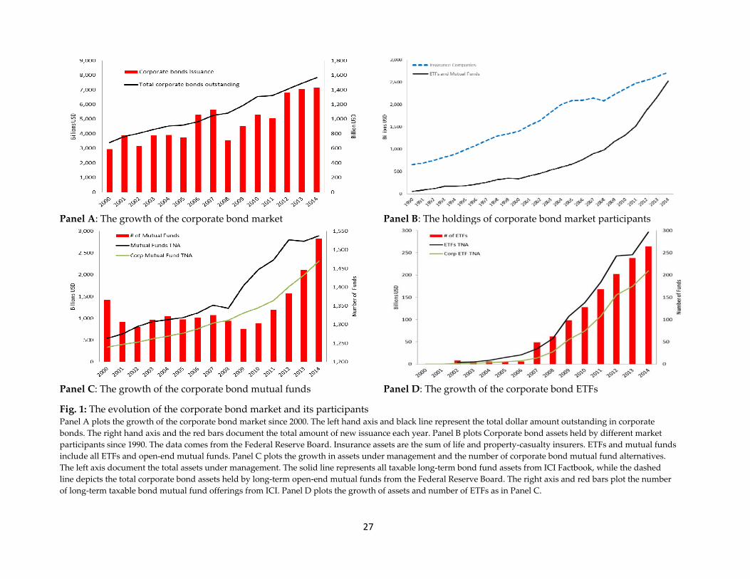
amount of corporate debt outstanding has increased 150% since 2000. Panel A of Figure 1 presents the 

growth in corporate bond assets outstanding and the annual issuance. 

[Insert Figure 1] 

Second,  regulatory  pressure  has  altered  the  dynamics  of  the  historically  opaque market. 

Traditionally,  broker‐dealers  held  large  inventories  in  order  to  facilitate  trades with  institutional 

investors,  the  majority  of  who  were  insurance  companies  and  pension  funds  characterized  by 

Bessembinder, Maxwell,  and Venkataraman  (2006)  as  long‐horizon  investors. Bid‐ask quotes  and 

transaction  prices were  not  readily  available  until  the  introduction  of  the  Trade  Reporting  and 

Compliance  Engine  (TRACE)  in  July  2002. Despite  the  introduction  of  delayed  trade  reporting, 

Bessembinder,  Maxwell,  and  Venkataraman  (2006),  Edwards,  Harris,  and  Piwowar  (2007)  and 

Goldstein,  Jiang, and Ng  (2015) all document  that corporate bonds  trade  infrequently, particularly 

relative to equities and other fixed income investments. Pressured by increased capital requirements 

the broker‐dealer  inventory has decreased by more  than 50%  (Dick‐Nielsen and Rossi, 2016). The 

impact of traditional market makers withdrawal on liquidity is uncertain with practitioners claiming 

that markets are  increasingly  illiquid and Anderson and Stulz  (2017) and Bao, O’Hara, and Zhou 

(2016) finding evidence of greater illiquidity in periods of stress. Conversely, Bessembinder, Jacobsen, 

Maxwell, and Venkataraman (2016) find that liquidity is not significantly lower since the crisis, but 

that the traditional commitment structure is changing. 

Third, as  the corporate bond market structure has evolved, nontradional  investors, mutual 

funds and ETFs have emerged as  increasingly  important  investors.6 The accumulation of assets by 

                                                            6 Bloomberg documents the change in the post‐crisis bond market model as a transition of power from banks to mutual funds, 

hedge funds, and exchange traded funds. They state that regulations have paved the way for the buy‐side “to exert more influence 

than ever on markets.” See: https://www.bloomberg.com/news/features/2016‐08‐15/the‐rise‐of‐the‐buy‐side  

9  

these funds, whose  investment strategy and  investor base  is significantly different  than  traditional 

investors  has  implications  for  the  underlying market  because  of  the  liquidity  they  provide  their 

investors and thus the liquidity they may demand. Panel B of Figure 1 plots the Federal Reserve Board 

data on the amount of corporate and foreign bonds held by two groups. The figure shows that the 

assets held by mutual funds and ETFs are now equal to those of insurance companies. Panels C and 

D of Figure 1 present details on the growth of mutual funds and ETFs, including the number of funds 

and assets under management of all  long‐term  taxable bond  funds  from  ICI FactBook, as well as, 

corporate bond specific assets from the Federal Reserve Board. From these figures it is evident that a 

large portion of growth in these investment vehicles has occurred since 2009 with the corporate bond 

assets of mutual funds doubling and ETF corporate bond assets quadrupling. 

Given  the  focus of  this paper on mutual  funds and ETFs, an extended discussion of  their 

structures is needed. At the most basic level, mutual funds and ETFs are investment vehicles backed 

by a basket of corporate bonds. Mutual funds are distinguished by their investment mandate as either 

active mutual  funds, who  attempt  to  outperform  their  benchmark,  or passive mutual  fund, who 

attempt to replicate their benchmark. Regardless of the type of mutual fund, investors are provided 

with daily liquidity. That is an investor can submit a buy or sell order for the mutual fund shares at 

any point throughout the day and all transactions will occur at the closing NAV. 

Corporate bond ETFs, the first of which was introduced in June 2002, are a hybrid between 

traditional open‐end mutual funds and closed end funds (CEFs). The unique features of ETFs allows 

them to offer lower management fees, greater transparency, and tax efficiencies to attract investors 

(Poterba  and  Shoven,  2002). ETFs provide  liquidity  to  investors  in  two  venues,  the primary  and 

secondary markets. The primary market is used by ETFs to handle liquidity shocks in the secondary 

market, to ensure that orders are filled, and to arbitrage excessive market price deviations from NAV. 

This market is the direct channel linking ETFs to the underlying. It involves large transactions between 

APs  and  the  fund  sponsor  through  the  in‐kind  creation  and  redemption process.  In  contrast,  the 

creation and redemption process of mutual funds occurs between the fund and individual investors 

as an exchange of cash for individual units of the underlying basket. The secondary market of ETFs, 

is where buyers and sellers of  the ETF  transact directly on  the equity exchange without any  fund 

involvement. It is possible that investors with access to the corporate bond market can also engage in 

risky arbitrage between the secondary ETF market and the underlying market. 

10  

In Table 1 we present summary statistics for mutual funds in Panel A and ETFs in Panel B. 

While the holdings of mutual funds and ETFs have similar duration and credit quality, the distribution 

of fund characteristics validates the common refrain surrounding ETFs relative to mutual funds. For 

instance, ETFs have expense ratios and turnover that are more than half of the mean level of mutual 

funds reflecting the relative simplicity of ETF management. In addition, ETFs have a much greater 

percentage of fund assets invested in corporate securities that mutual funds and lower levels of cash 

and government bond investments. Interestingly, the mean assets under management of ETFs is lower 

than mutual funds, while the median is significantly lower, reflecting the concentration of ETF assets 

in the largest funds. 

2.2. The Taper Tantrum as an exogenous shock to fund flows 

An empirical challenge of identifying potential vulnerabilities created by this new corporate 

bond  market  regimen  is  the  absence  of  market  shocks  and  resultant  fund  flows  during  the 

unprecedented bond market since the financial crisis. Nevertheless, the Taper Tantrum of the summer 

of  2013  serves  as  our  exogenous  market‐wide  shock.  Prior  to  this  event,  bond  funds  saw 

disproportionate  inflows  relative  to  other  asset  classes  as  the  Federal  Reserve  employed 

unprecedented policy initiatives such as open market purchases of government bonds and mortgage‐

backed securities, a process commonly referred to as quantitative easing (QE). The QE program  in 

place since November of 2008 was intended to lower long‐term interest rates in an effort to bolster 

housing  markets,  employment,  and  real  activity.  Following  positive  economic  developments, 

Chairman Ben Bernanke testified on May 22, 2013 that the Federal Reserve would likely begin slowing 

or tapering the pace of its bond purchases conditional on continued economic stability. On June 19, 

2013 the Chairman held a news conference to document the economic justification for the purchase 

slowdown. Convinced  that  the end of QE was near,  the market responded by selling assets,  in an 

episode commonly compared to a tantrum. Between May 21, 2013 and the beginning of September 

both  the  five‐  and  ten‐year Treasuries  increased over  100 basis points. Beyond  the Treasury  rate, 

investors anticipating a sharp reevaluation of risk took advantage of the liquidity provisions of mutual 

funds and ETF by swiftly withdrawing assets. According to Trim Tabs Investment Research, a record 

$69 billion was withdrawn from bond mutual fund and ETFs in June 2013, with outflows continuing 

11  

throughout July and August. The period of uncertainty was resolved on September 18, 2013 when the 

Fed officially announced it would wait to begin scaling back the QE program.  

[Insert Figure 2] 

3. Data 

Our corporate bond fund data begins in January 2010, in order to study a period in which the 

assets managed by these two investment vehicles is no longer negligible, and ends in March 2015. We 

begin by identifying corporate bond funds using the Center for Research in Security Prices (CRSP) 

Survivor‐Bias‐Free US Mutual Fund Database. In particular, we denote any mutual fund or ETF that 

as an average corporate bond weighting of twenty percent or greater as a corporate bond fund. We 

also collect fund characteristics from the Morningstar Mutual Fund Database, including the number, 

the concentration, the average duration, and the average credit quality of the bond holdings. Matching 

on  fund cusip, we  then use CRSP  to obtain  fund holdings, monthly  returns, monthly  fund assets, 

turnover, expense ratio, and share class data. Furthermore, we use the CRSP database to distinguish 

ETFs from mutual funds and to distinguish active and index mutual funds. Using this data we follow 

the literature to compute the flow to each fund,  , in month,  , as 

,, , ∗ 1 ,

, 

For mutual funds with multiple share classes we aggregate data at the portfolio level by summing 

fund assets, and value weighting other characteristics.  

We  use  the  Trade  Reporting  and  Compliance  Engine  (TRACE)  database  to  obtain  bond 

transaction data. Using the method of Dick‐Nielsen (2009), we filter out possibly erroneous trades. We 

compute the monthly spread of bond   from issuer   in month  ,  , ,  as the volume weighted 

average yield reported for all transactions in a month over the maturity‐matched Treasury rate. We 

also use the TRACE database to compute the our liquidity proxy,  , ,  developed by Amihud 

(2002), which measures the price impact of a $1 million trade. Specifically, for bond   from issuer   in 

month   the proxy is computed as the median of the daily measure 

,1 | |

∗ 10 , 

(1) 

(2) 

12  

where   is the number of returns on day d, rj is the return of consecutive transactions, and   is the 

dollar volume of a trade. This measure can be interpreted as the basis points price movement per one 

million  dollars  of  traded  volume.  Bond  characteristics  come  from  the Merchant  Fixed  Income 

Securities Database (FISD) and are merged on eight‐digit CUSIP. In addition, for each bond we create 

an average rating using numerical conversions of Standard & Poor’s (S&P) ratings.  

  Finally, we obtain the daily shares outstanding of ETFs from Bloomberg. We use the shares 

outstanding to compute the Da and Shive (2013) creation and redemption  intensity measure,  , . 

The measure is calculated using the shares outstanding for the set ETFs  in month   as  

, ,

,. 

Creation and redemption could drive underlying liquidity because authorized participants need to 

compile or sell baskets of the underlying security to maintain the ETF. The activity associated with 

CRI reflects the direct involvement of the affiliates of the ETF in a bond. 

4. Methodology and results 

This section details the methodology and presents the results on the impact of Taper Tantrum 

flows to mutual funds and ETFs on the yield spreads of associated bonds. We begin by considering 

the yield spread effects of each investment vehicle and then examine three potential explanations for 

our main results.  

4.1. The yield spread effect of mutual funds and ETFs 

Our empirical analysis begins by examining if outflows during the summer of 2013 following 

the Federal Reserve announcement, have an impact on the pricing of constituent bonds. We follow 

the methodology of Coval and Stafford (2007) and Mitchell, Pulvino, and Stafford (2004), by running 

the  tests  over  several months  to  look  at  cumulative  returns  and  subsequent  reversals  to provide 

evidence of a non‐fundamental shock to prices.  Specifically, for each investment vehicle in each of the 

t months following the summer of 2013, we run the regression  

(3) 

13  

,

, , , ,

, , ,

, ∗

∗ , , . 

The dependent variable, ,,  is  the  change  in  the volume‐weighted average 

yield of bond,  i,  from  issuer  j over  the maturity‐matched Treasury  rate. The  change  is measured 

relative to the bond’s volume‐weighted yield in May excluding all transactions post May 21, the day 

prior to Bernake’s testimony.  

The  covariate of  interest  is  , ,  the weighted‐average monthly  flow  for 

either all mutual funds or all ETFs that report bond i as a holding prior to the onset of the event. We 

multiply the measure by ‐1 to help with interpretation of the coefficient of interest,  , which measures 

the impact of Tantrum outflows to either mutual funds or ETFs on a bond’s yield spread relative to 

pre‐event levels. To be included in the regression we require the weighted average flow to be negative, 

i.e. an outflow. The square of  , , is used to control for any potential nonlinearities 

in the relationship of interest 

As in Manconi et al. (2012), the inclusion of issuer fixed effects,  addresses endogeneity issues 

associated with changes in the fundamentals of an issuer. The use of issuer fixed effects, controls for 

any differential changes in firm fundamentals during our turmoil event by allowing us to effectively 

compare the change in yield spreads of bonds from the same issuer subjected to different levels of 

fund induced pressures. Therefore, if a firm has only one outstanding issue subjected to outflows, it 

automatically drops out of the analysis. 

We also include a vector of bond specific characteristics set to their pre‐event levels to control 

for differences  in  issues  from  the same  firm. We control  for  the  log of  the  issue size  in millions of 

dollars,  Log(Size),  the  number  of  years  left  to maturity  and  its  square,  Time  to Maturity,  and  the 

liquidity  level of  the  issue using  the Amihud  illiquidity measure, Amihud. The yield spread of  the 

bond prior  to  the event,    is also used  to account for differences  in bonds from  the same 

issuer that are not captured by our other controls, for instance differences in covenants. Finally, we 

(4) 

14  

include interactions to account for the likelihood that investors sell bonds with higher interest rate 

exposure,  ∗ ,  and  greater  liquidity,  ∗

. 

Using equation (4), we run the regression for mutual funds and ETFs separately to identify 

the impact of each investment vehicle on their underlying bonds. Table 2 presents the results for ETFs 

in  Panel A  and mutual  funds  in  Panel  B.  The  results  show  that  there  is  no  significant  effect  or 

distinguishable  pattern  for  mutual  fund  outflows.  Conversely,  ETF  outflows  drive  spreads 

significantly  higher  for  up  to  seven months  beyond  the  event.  In  September  2013,  as  the  Taper 

Tantrum  subsided, bonds with  a one percentage  increase  in  exposure  to ETF outflows had yield 

spreads 8.7 basis points higher  than a bond from  the same  issuer. This corresponds  to a 12.6 basis 

point  increase  in yield spread relative  to bonds  from  the same  issuer  for a one standard deviation 

greater exposure  to ETF outflows during  the  summer of 2013. Economically,  this  implies a 10.7% 

increase in the yield spread of the average corporate bond in our sample. The statistical significance 

in the difference diminishes after seven months with yield spreads reverting to their pre‐crisis level.  

[Insert Table 2] 

In Figure 3, we plot the impact of a one standard deviation outflow to ETFs in Panel A and 

mutual funds on Panel B on the yield spread of bonds in our regression. The figure shows the impact 

of outflows during the Taper Tantrum period peaking in September for bonds held by ETFs and the 

effect lasting through March of 2014. According to Coval and Stafford (2007) if these yield changes are 

due to changes in fundamentals, the yields should remain permanently higher. Together the higher 

yield spreads and the reversion suggests that ETFs put temporary pressure on bonds, pushing yields 

beyond their fundamental levels. Therefore the evidence suggests that changes in yield spreads can 

be attributed to price pressure created by outflows to ETFs. Panel B shows that there is little statistical 

significance between mutual fund outflows in the Taper Tantrum and the yield spread of their bonds. 

[Insert Figure 3] 

4.2. Examining the differential effect of mutual funds and ETFs 

The main results of this paper are particularly intriguing given the size and youth of the ETF 

market relative to the larger and more mature mutual fund market. The differential effect identified 

15  

suggests the distinguishing features of ETFs may be a source of potential fragility for the corporate 

bond market. In this subsection we focus on three distinctive features of ETFs in an attempt to identify 

the source of the ETF induced yield pressure. Specifically, we examine if the index based nature of 

most ETFs, differences in investor bases, or implications of the creation and redemption mechanism 

can help to explain the differential impact of flows during a period of turmoil on the underlying bonds. 

4.2.1. Index based funds 

For nearly a decade, investors have poured money into index based vehicles and away from 

actively managed funds. ETFs have been a key beneficiary of this investment theme, as nearly all ETFs 

focus on replicating the returns of a pre‐specified benchmark rather than outperformance. While an 

index  strategy  reduces  the work  required  of  a manager,  it  also  constrains  her  response  to  flows 

(Christoffersen, Keim, and Musto, 2008; Elton, Gruber, and Busse, 2004). Unlike active managers who 

can  use  discretion  in  selecting which  assets  to  trade  in  response  to  flows,  index managers  are 

mandated  to buy and sell  index bonds  in amounts determined by  their benchmark weighting. Of 

greatest relevance to this paper, active managers may response to redemptions by trading bonds in 

which they will have the lowest price impact.  

Most equity index funds utilize a strict indexing strategy because the benchmarks they follow 

have a limited number of constituents, which trade frequently. In contrast, fixed income index funds 

generally employ a representative sampling strategy, selecting only a subset of index bonds to best 

match  the characteristics of  the  index. While  representative sampling does  increase  the manager’s 

ability  to  selectively  respond  to  flow,  it  remains  possible  that  the  index‐based  nature  of  ETFs  is 

responsible for the flow‐induced yield pressure. If the passive nature of ETFs contributed to the results 

documented above, we would expect similar yield pressure from index mutual funds who follow the 

same mandate. To examine if the ETF yield pressure results can be attributed to their index strategies, 

we break down  the mutual  fund universe  into active and  index  funds. We  then execute  the same 

regression  in Eq. (4) for  the  two subsets. Table 3 presents  the results for outflows  to active mutual 

funds in Panel A and index mutual funds in Panel B. 

[Insert Table 3] 

16  

The results of Table 3 show that outflows from neither active nor index mutual funds have a 

significant  impact on  the yield  spread  change of  their  constituent  corporate bonds. Therefore, we 

conclude  that  the  reduced  flexibility  of  index  fund management  is  not  responsible  for  the  yield 

pressure of ETFs. Instead, we continue by investigating other structural and operational features that 

influence the clientele and construction of these investment vehicles as potential sources of fragility. 

4.2.2. The horizon of investors 

ETFs  are  often  described  as mutual  funds  that  trade  intraday  on  an  exchange.  This  key 

structural feature has appealed to investors of all types as evidenced by the outsized secondary market 

volumes of corporate bond ETFs. Chordia (1996), Deli and Varma (2002) and Nanda, Narayanan, and 

Warther (2000) theorize that different fund structures may be utilized to appeal to the heterogeneous 

needs of  investors.  In particular, Nanda, Narayanan, and Warther  (2000) show  that  in equilibrium 

different fund structures and fees are used by managers exposed to a systematic liquidity shock to 

attract investors with different liquidity needs. Together with Chordia (1996), they show that different 

structures are used by mutual funds to screen out high liquidity demand investors, whose frequent 

trading  exposes  more  stable  investors  to  trade  induced  externalities.  Moreover,  Amihud  and 

Mendelson  (1986) and Constantinides  (1986) predict  that short‐term  investors self‐select  into more 

liquid  assets.  Considering  these  theories  and  the  predictions  of  Poterba  and  Shoven  (2002), we 

hypothesize that ETFs are more likely to attract short‐horizon traders. 

Short‐horizon  investors are  theorized by Allen, Morris, and Shin  (2006), De Long, Shleifer, 

Summers, and Waldmann (1990a), Dow and Gorton (1994), Froot, Scharfstein, and Stein (1992), Morris 

and Shin (2004) and Stein (2005) to specialize in investment strategies that focus not on fundamentals, 

but instead on the expected behavior of other investors. Cespa and Vives (2015) show that in normal 

market conditions, where liquidity shocks are persistent short‐horizon investors will not impact asset 

prices. However, their presence can be destabilizing if as predicted by Allen, Morris, and Shin (2006), 

Bernardo and Welch (2004) and Morris and Shin (2004) in periods of turmoil short‐horizon investors 

are  expected  to  trade  simultaneously  and  place  a  disproportionate  weight  on  a  public  signal. 

Bhattacharya and O’Hara (2016) show that ETFs can expose the underlying to rational herding, where 

speculators herd on the same systematic signal, which may lead to market fragility in hard to trade 

underlying assets. 

17  

To examine if ETFs appeal to a different investor base we first seek to describe the distribution 

of flows to the different investment vehicles. Table 4 presents the flows to the different fund types and 

their distribution during both the Taper Tantrum and non‐Taper Tantrum periods. The table provides 

preliminary  evidence  that ETFs attract a more active  investor base with volatility of  flows nearly 

double that of all mutual funds. During the Taper Tantrum event ETFs in the lowest decile of flow 

experienced outflows nearly four times greater than those in normal market conditions. 

[Insert Table 4] 

The  literature  suggests  that one way  in which  short‐horizon  investment  can be  a  source of 

fragility is if these investors engage in positive feedback trading, buying when the market is moving 

higher and selling when the market is moving lower. De Long, Shleifer, Summers, and Waldmann 

(1990b) present a model of investors who trade on past price trends and show that a result of their 

presence  is price  destabilization.  To  test  if  these  new  corporate  bond  investors  follow  a  positive 

feedback strategy, we follow Edelen and Warner (2001), Goetzmann and Massa (2003) and Warther 

(1995) by examining the sensitivity of investors to lagged market returns over the period from January 

2010 to March 2015. Since interest rates dictate the price of the underlying corporate bonds, we test if 

ETFs are more likely to respond using the following specification 

, ∆ ⁄ ∗ ∆ ⁄ , , . 

The dependent variable in the above regression,  , , is the monthly flow to fund   in month  . 

Δ /  is the change in either the one‐ or five‐year treasury rate in the prior month normalized by its 

standard deviation. We also control for the average effective duration and rating of the fund’s holding, 

as well  as,  the  expense  ratio,  turnover,  and  one‐,  two‐,  and  three‐month  lagged  fund  flows. The 

coefficient of interest,  , on the interaction Δ ⁄ ∗ , measures the differential behavior of ETF 

investors. Table 5 shows the results of these tests. 

[Insert Table 5] 

The coefficient on Δ ⁄ shows  that after controlling  for other  factors  lagged changes  in  interest 

rates are not a determinant of mutual  fund  flows. Meanwhile,  the  coefficient on  the ETF dummy 

suggest that this investment vehicle has larger inflows over the 2010 to 2015 period. Interestingly, the 

coefficient  on  the  interaction  is  negative  and  significant  for  both  one‐  and  five‐year  interest  rate 

(5) 

18  

changes  suggesting  that  ETF  investors  are more  likely  to  demand  liquidity when  interest  rates 

increased in the previous month. In particular, a one‐standard deviation in the one‐year Treasury rate 

leads to 0.09% higher outflows for ETFs than for mutual funds. These results show that ETF investors 

are more likely to trade in response to interest rate changes, suggesting they are more likely to follow 

potentially destabilizing positive feedback trading strategies.  

Overall,  this subsection documents  that ETF  investors have shorter horizons  that mutual  fund 

investors. In normal markets, the secondary market feature of ETFs should prevent the introduction 

of this new investor type from impacting the underlying. Nevertheless, the presence of these traders, 

combined with the main findings that ETF outflows led to higher yield spreads for exposed bonds 

suggest  that  the  liquidity  illusion of ETFs  is a potential  source of  fragility  for  the  corporate bond 

market. 

4.2.3. The implications of the creation and redemption mechanism 

The key operational difference between mutual funds and ETFs is the reliance of the latter on 

in‐kind creation and  redemption, which has  important  implications  for portfolio construction and 

arbitrage that differentiate ETFs and mutual funds. First, despite having an investor base of liquidity 

demanders ETFs may have a reduced incentive to manage a liquidity buffer since they do not need to 

produce cash on demand to meet the flows of investors. In contrast, mutual fund managers rely on 

liquid holdings during volatile times to reduce the externalities associated with the adverse effect of 

investor  flows as documented by Chen, Goldstein, and  Jiang  (2010) and Liu and Mello  (2011). For 

corporate  bond managers,  the  liquidity  buffer  consists  of  cash,  cash  equivalents,  and  the more 

frequently traded government bonds (Goldstein, Jiang, and Ng, 2015). In Table 6, we present the mean 

and median assets  allocated  to  cash, government bonds,  corporate bonds,  and  securitized bonds. 

Panel A presents  the comparison of mutual  funds and ETFs. The evidence suggests  that  there  is a 

statistically significant difference in the portfolio construction techniques used by the two investment 

vehicles. The median mutual fund holds 8.38% and 13.34% of its assets in cash and government bonds, 

respectively,  leaving  just 45.44%  to allocate  to corporate bonds.  In sharp contrast,  the median ETF 

holds just 2.40% in cash and 0.34% in government bonds, allowing for the funds to invest over 93% of 

their assets in corporate bonds. In Panel B, we present the portfolio allocations for mutual funds and 

ETFs in the lowest quartile of tantrum flows, i.e. those with the greatest outflows. For these funds, the 

19  

lower cash and higher corporate bond levels of ETFs remain statistically significant for both the mean 

and median funds. However, the difference in government holdings is no longer significant and only 

economically  interesting  for  the median  values.  Finally, Panel C  compares  the holdings  of  index 

mutual funds and ETFs. The results of this comparison are similar to those documented above with 

one key distinction. While, the liquidity buffer of the median index fund comprises 47.83% of assets, 

it has a greater representation of government securities than in the broader mutual fund population. 

The presence of the liquidity buffer helps to explain to absence of any flow‐induced price pressure in 

corporate bonds from mutual funds. Managers can utilize their liquidity buffer to meet redemption 

requests without selling corporate bonds at potentially distressed prices, similar to the financial crisis 

period results of Hoseinzade (2015). Nevertheless, we do not rule out that the liquidity management 

techniques of mutual fund managers would be sufficient  in a prolonged market shock  in  this new 

corporate bond market regimen.  

[Insert Table 6] 

Another consequence of the creation and redemption mechanism is that APs can engage in 

arbitrage between  the market price of  the ETF and  the NAV of  the underlying.  In normal market 

conditions  and  for  ETFs  backed  by  assets  that  are  not  hard  to  trade,  arbitrage  occurs  nearly 

instantaneously. However, a difference in the two prices may occur and persist if limits to arbitrage 

such as of noise trader risk (De Long, Shleifer, Summers, and Waldmann, 1990a), synchronization risk 

(Abreu  and  Brunnermeier,  2003),  liquidation  risk  (Shleifer  and  Vishny,  1997),  transaction  costs 

(Pontiff, 1996), and short sale constraints (Ofek and Richardson, 2003) are present. Further, a number 

of theories suggest that in the presence of these limits arbitrage may actually amplify fundamental 

shocks (Greenwood and Thesmar, 2011; Hong, Kubik, and Fishman, 2012; Hugonnier and Prieto, 2015; 

Kyle and Xiong, 2001).  

We  begin  our  study  of  the  impact  of  imperfect  arbitrage  during  a  period  of  turmoil  on 

constituent bonds, by documenting the existence of persistent arbitrage opportunities. First, we split 

our ETF sample into two groups based on the average monthly percentage price to NAV deviation 

during the turmoil period computed as 

,, ,

,.  (6) 

20  

We then denote ETFs with the largest average Tantrum period discount, i.e. the ETF price falls below 

the NAV, as the high arbitrage exposure group. Figure 4 plots the average deviation of these high 

arbitrage exposure ETFs over time. The Figure shows that these ETFs previously traded above their 

NAV before the ETF price fell significantly below the NAV during the Taper Tantrum, reflecting the 

mass  exodus  experienced  in  anticipation of unexpectedly higher  interest  rates. The ETF discount 

bottoms in August 2013 before converging in March 2014.  

[Insert Figure 4] 

In Table 7 we compare the difference between observable characteristics for the high arbitrage 

exposure and the low arbitrage exposure ETFs. The credit quality of ETF holdings, the volatility of 

fund flows, and institutional ownership are not significantly different for the two groups. However, 

the  average  duration  of  the  high  arbitrage  exposure  group  is  significantly  higher, which  is  not 

surprising given that ETFs holding these bonds were under pressure in expectation of higher interest 

rates. Representative of common limits to arbitrage, the high arbitrage exposure group has higher bid‐

ask  spreads, higher  turnover, and  fewer assets under management. Despite  these differences,  the 

creation and redemption intensity measure, which proxies for the amount of arbitrage undertaken by 

APs  is  insignificantly different during normal market  conditions. However, during  the period  of 

turmoil arbitrage in the high exposure group drops while it is nearly unchanged in the low arbitrage 

exposure group. The difference in arbitrage intensity between the groups during the Taper Tantrum 

is  significant  suggesting  that  the  arbitrage mechanism  of  the high  exposure  group was  impaired 

during the event. 

[Insert Table 7] 

The existence of these arbitrage opportunities translates into potential selling pressure for the 

individual bonds. Therefore, we posit that bonds exposed to ETFs that experience significant selling 

pressure  and  for  which  arbitrage  is  impaired  were  subjected  to  greater  selling  pressure  by 

arbitrageurs, who are insensitive to the fundamental price of the bond. To test if impaired arbitrage is 

a potential source of the yield pressure and reversion, we form two portfolios at the end of the tantrum 

episode  based  on  the  exposure of  individual  bonds  to  arbitrage.  Specifically,  for  each  bond  i we 

21  

compute the ownership‐weighted average deviation of the set of K ETFs that hold bond during the 

Taper Tantrum as,  

,∑ , ∗ ,

∑ ,. 

In the measure  ,  is the amount of bond i held by ETF k in the holdings period prior to the onset 

of  the  tantrum episode and  ,   is  the average deviation of ETF k during  the Taper 

Tantrum months. 

Using this measure we divide the entire sample of bonds into high and low discount exposure 

portfolios. The high discount exposure portfolio includes all bonds with exposure measure of Eq. (7) 

less than the median value. We then track the yield spread of these two portfolios until the end of our 

sample in March 2015 in Panel A of Figure 5. As you can see from this Figure, the yield spreads of the 

two portfolios are  close during  the period of  turmoil, but begin  to diverge as  the Taper Tantrum 

concludes  and  limits  to  arbitrage  dissipate. As  arbitrageurs  reentered  the market  by  selling  the 

underlying and buying the ETF, the yield spreads of high exposure to ETF discount bonds are pushed 

above those without similar arbitrage pressure. In Panel B of Figure 5, we present the difference in the 

yield spreads for the two portfolios and the t‐statistics of the difference. The pattern of the differences 

shows the yield spreads of high exposure bonds increasing significantly before reverting in July 2014, 

suggesting  that arbitrageurs  serve as a  shock propagation mechanism  from  the  liquid ETF  to  the 

underlying bonds. The timeline for the convergence of the two portfolios coincides with the closing 

of the arbitrage opportunity shown in Figure 4 supporting our hypothesis that the non‐fundamental 

move in prices can be partially attributed to arbitrage. 

[Insert Figure 5] 

To formally test the impact of impaired ETF arbitrage on constituent corporate bonds, we run 

both univariate and multivariate regressions. Corresponding  to Figure 5, we  first run a univariate 

specification  of  the  yield  spread  level  of  bond  i  in  month  t  on  the  high  exposure  dummy, 

, . We  also  run  the  following multivariate  specification  to 

control for bond level characteristics,  

, , ,

, , ,  

(7) 

(8) 

22  

Table 8 presents the results of the univariate test in Panel A and the multivariate test in Panel 

B. Focusing on the multivariate specification shows that after controlling for observable characteristics 

of bonds, there is no significant difference between the yield spread levels of bonds with high exposure 

to ETF arbitrage during the tantrum period. This suggests that as the price of the ETF moved lower, 

the yield spreads of exposed constituents did not  react significantly different  to  the change  in  the 

markets expectations of interest rates. Rather, it was after the turmoil and limits to arbitrage subsided, 

that those bonds most exposed to arbitrage opportunities created by extreme selling pressure in the 

ETF move  significantly higher. Specifically,  the yield  spreads of bonds  exposed  to high  arbitrage 

trading are 14.2 basis points higher in September than those from the low arbitrage exposure group. 

The difference  in yield spreads peaks  in December 2013 and completely reverts  to an  insignificant 

level by July 2014. 

[Insert Table 8] 

The results of this subsection show that the unique creation and redemption mechanism of 

ETFs has significant  implications for the asset prices of constituent bonds. First, we document that 

mutual funds utilize a liquidity buffer to respond to temporary periods of turmoil, such as the Taper 

Tantrum studied in this paper. For ETFs the in‐kind mechanism reduces the funds’ reliance on the 

buffer and allows for greater investment in constituent bonds. However, when arbitrage is limited the 

liquidity  of  the  ETF  relative  to  the  illiquidity  of  the  underlying may  create  persistent  arbitrage 

opportunities that allow for a market‐wide shock to propagate to exposed bonds. In particular, we 

show  that  bonds  held  by  ETFs  subjected  to  selling  pressure  during  the  Taper  Tantrum  have 

significantly higher yield spreads as arbitrageurs reenter the market leading to the convergence of the 

ETF price and NAV, but pushing the constituent yield spreads beyond fundamental levels before they 

revert as arbitrage pressure abates.  

5. Conclusion 

The  corporate  bond market  long  dominated  by  broker‐dealers  and  long‐term  investors,  such  as 

insurance companies, has seen its primary market makers withdraw and new more liquid forms of 

innovation  emerge.  This  paper  uses  an unexpected  increase  in  the  interest  rates  and  subsequent 

outflows from ETFs and mutual funds, in an event known as the Taper Tantrum, to cleanly identify 

the impact of outflows to these investment vehicles on bond yields. Comparing bonds from the same 

23  

issuer, we find that ETF outflows lead to significantly higher yield spreads in the months following 

the shock, with the impact lasting seven months. The significance and pattern of the coefficients of 

our regression indicate that ETFs contribute to flow‐induced yield spread pressure in the corporate 

bond market. There is no significant relationship between Tantrum period outflows to mutual funds 

and subsequent changes in yield spreads.  

We  further  investigate  the differences between ETFs and mutual  funds and show  that  the 

contrasting findings for can be attributed to the structural and operational features of ETFs. We first 

rule out that the index‐based mandate of ETFs is responsible for the pattern indicative of flow‐induced 

yield  pressure  by  documenting  that  index mutual  funds  do  not  have  a  similar  effect  on  their 

constituent bonds. Second, we show that ETFs and mutual funds appeal to a different investor base, 

with the greater flow volatility of ETFs suggestive of shorter‐horizon investors. Further, ETF flows 

more  sensitive  to  changes  in  interest  rates,  implying  that  these  new  investors  in  corporate  bond 

markets may engage  in potentially destabilizing positive  feedback  trading. Third, we consider  the 

portfolio construction and arbitrage implications of the in‐kind creation and redemption mechanism 

used by ETFs. We document that mutual funds have a significant liquidity buffer. The lack of flow‐

based yield pressure for mutual funds  in  this  turmoil period suggests  that fund managers utilized 

their  liquidity  buffer  to meet  redemption  requests without  selling  corporate  bonds  at potentially 

distressed prices, similar to the financial crisis results of Hoseinzade (2015). Nevertheless, we do not 

rule out that the liquidity management techniques of mutual fund managers would be sufficient in a 

prolonged market shock in this new corporate bond market regimen. For ETFs the in‐kind mechanism 

reduces  the  funds’  reliance on  the buffer and allows  for greater  investment  in  constituent bonds. 

However, when arbitrage is limited the liquidity of the ETF relative to the illiquidity of the underlying 

may  create persistent arbitrage opportunities  that allow  for a market‐wide  shock  to propagate  to 

exposed bonds. In particular, we show that bonds held by ETFs that trade at significant discounts to 

their NAV due to selling pressure during the Taper Tantrum have significantly higher yield spreads 

as arbitrageurs reenter the market leading to the convergence of the ETF price and NAV, but pushing 

the  constituent  yield  spreads  beyond  fundamental  levels  before  they  revert  as  arbitrage pressure 

abates.  

24  

References 

Abreu, D., Brunnermeier, M., 2003. Bubbles and Crashes. Econometrica 71, 173–204. 

Allen, F., Morris, S., Shin, H.S., 2006. Beauty contests and iterated expectations in asset markets. 

Review of financial Studies 19, 719–752. 

Amihud, Y., 2002. Illiquidity and stock returns: cross‐section and time‐series effects. Journal of 

Financial Markets 5, 31–56. 

Amihud, Y., Mendelson, H., 1986. Asset pricing and the bid‐ask spread. Journal of Financial 

Economics 17, 223–249. 

Anderson, M., Stulz, R.M., 2017. Is Post‐Crisis Bond Liquidity Lower? National Bureau of Economic 

Research. 

Bao, J., O’Hara, M., Zhou, X.A., 2016. The Volcker rule and market‐making in times of stress. 

Bernardo, A.E., Welch, I., 2004. Liquidity and financial market runs. The Quarterly Journal of 

Economics 119, 135–158. 

Bessembinder, H., Jacobsen, S.E., Maxwell, W.F., Venkataraman, K., 2016. Capital commitment and 

illiquidity in corporate bonds. 

Bessembinder, H., Maxwell, W., Venkataraman, K., 2006. Market transparency, liquidity 

externalities, and institutional trading costs in corporate bonds. Journal of Financial 

Economics 82, 251–288. 

Bhattacharya, A., O’Hara, M., 2016. Can etfs increase market fragility? effect of information linkages 

in etf markets. Working Paper. 

Cella, C., Ellul, A., Giannetti, M., 2013. Investors’ horizons and the amplification of market shocks. 

Review of Financial Studies hht023. 

Cespa, G., Vives, X., 2015. The beauty contest and short‐term trading. The Journal of Finance 70, 

2099–2154. 

Chen, Q., Goldstein, I., Jiang, W., 2010. Payoff complementarities and financial fragility: Evidence 

from mutual fund outflows. Journal of Financial Economics 97, 239–262. 

Chordia, T., 1996. The structure of mutual fund charges. Journal of Financial Economics 41, 3–39. 

Constantinides, G.M., 1986. Capital market equilibrium with transaction costs. Journal of Political 

Economy 94, 842. 

Coval, J., Stafford, E., 2007. Asset fire sales (and purchases) in equity markets. Journal of Financial 

Economics 86, 479–512. 

Da, Z., Shive, S., 2013. When the bellwether dances to noise: Evidence from exchange‐traded funds. 

Unpublished working paper. University of Notre Dame. 

De Long, J.B., Shleifer, A., Summers, L.H., Waldmann, R.J., 1990a. Noise trader risk in financial 

markets. Journal of political Economy 703–738. 

De Long, J.B., Shleifer, A., Summers, L.H., Waldmann, R.J., 1990b. Positive feedback investment 

strategies and destabilizing rational speculation. Journal of Finance 45, 379–395. 

Deli, D.N., Varma, R., 2002. Contracting in the investment management industry:: evidence from 

mutual funds. Journal of Financial Economics 63, 79–98. 

Dick‐Nielsen, J., 2009. Liquidity biases in TRACE. Journal of Fixed Income 19, 43. 

Dick‐Nielsen, J., Rossi, M., 2016. The cost of immediacy for corporate bonds. 

Dow, J., Gorton, G., 1994. Arbitrage chains. Journal of Finance 49, 819–849. 

Edelen, R.M., Warner, J.B., 2001. Aggregate price effects of institutional trading: a study of mutual 

fund flow and market returns. Journal of Financial Economics 59, 195–220. 

25  

Edwards, A.K., Harris, L.E., Piwowar, M.S., 2007. Corporate bond market transaction costs and 

transparency. Journal of Finance 62, 1421–1451. 

Froot, K.A., Scharfstein, D.S., Stein, J.C., 1992. Herd on the street: Informational inefficiencies in a 

market with short‐term speculation. The Journal of Finance 47, 1461–1484. 

Gennaioli, N., Shleifer, A., Vishny, R., 2012. Neglected risks, financial innovation, and financial 

fragility. Journal of Financial Economics 104, 452–468. 

Goetzmann, W.N., Massa, M., 2003. Index funds and stock market growth. Journal of Business 76, 1–

1. 

Goldstein, I., Jiang, H., Ng, D.T., 2015. Investor Flows and Fragility in Corporate Bond Funds. 

Available at SSRN 2596948. 

Greenwood, R., 2005. Short‐and long‐term demand curves for stocks: theory and evidence on the 

dynamics of arbitrage. Journal of Financial Economics 75, 607–649. 

Greenwood, R., Thesmar, D., 2011. Stock price fragility. Journal of Financial Economics 102, 471–490. 

Gromb, D., Vayanos, D., 2010. Limits of Arbitrage. The Annual Review of Financial Economics is 2, 

251–75. 

Hong, H., Kubik, J.D., Fishman, T., 2012. Do arbitrageurs amplify economic shocks? Journal of 

Financial Economics 103, 454–470. 

Hoseinzade, S., 2015. Do Bond Mutual Funds Destabilize the Corporate Bond Market? Unpublished 

working paper. Boston College. 

Hugonnier, J., Prieto, R., 2015. Asset pricing with arbitrage activity. Journal of Financial Economics 

115, 411–428. doi:http://dx.doi.org/10.1016/j.jfineco.2014.10.001 

Israeli, D., Lee, C.M., Sridharan, S., 2016. Is there a Dark Side to Exchange Traded Funds (ETFs)? An 

Information Perspective. Unpublished working paper. Stanford University. 

Kyle, A.S., Xiong, W., 2001. Contagion as a wealth effect. The Journal of Finance 56, 1401–1440. 

Liu, X., Mello, A.S., 2011. The fragile capital structure of hedge funds and the limits to arbitrage. 

Journal of Financial Economics 102, 491–506. 

Malamud, S., 2016. A dynamic equilibrium model of ETFs. 

Manconi, A., Massa, M., Yasuda, A., 2012. The role of institutional investors in propagating the crisis 

of 2007–2008. Journal of Financial Economics 104, 491–518. 

Mitchell, M., Pulvino, T., Stafford, E., 2004. Price pressure around mergers. Journal of Finance 59, 31–

63. 

Morris, S., Shin, H.S., 2004. Liquidity black holes. Review of Finance 8, 1–18. 

Nanda, V., Narayanan, M., Warther, V.A., 2000. Liquidity, investment ability, and mutual fund 

structure. Journal of Financial Economics 57, 417–443. 

Ofek, E., Richardson, M., 2003. Dotcom mania: The rise and fall of internet stock prices. The Journal 

of Finance 58, 1113–1137. 

Pan, K., Zeng, Y., 2017. Arbitrage under liuquidity mismatch: Theory and evidence from authorized 

participants of bond ETFs. 

Pontiff, J., 1996. Costly Arbitrage: Evidence from Closed‐End Funds. The Quarterly Journal of 

Economics 111, 1135–1151. 

Poterba, J.M., Shoven, J.B., 2002. Exchange‐Traded Funds: A New Investment Option for Taxable 

Investors. American Economic Review 92, 422–427. 

Schmidt, L., Timmermann, A., Wermers, R., 2016. Runs on money market mutual funds. The 

American Economic Review 106, 2625–2657. 

Shleifer, A., Vishny, R.W., 1997. The limits of arbitrage. The Journal of Finance 52, 35–55. 

26  

Stein, J.C., 2005. Why are most funds open‐end? Competition and the limits of arbitrage. The 

Quarterly journal of economics 120, 247–272. 

Warther, V.A., 1995. Aggregate mutual fund flows and security returns. Journal of financial 

economics 39, 209–235. 

 

 

27  

   Panel A: The growth of the corporate bond market  Panel B: The holdings of corporate bond market participants 

 Panel C: The growth of the corporate bond mutual funds  Panel D: The growth of the corporate bond ETFs    

Fig. 1: The evolution of the corporate bond market and its participants Panel A plots the growth of the corporate bond market since 2000. The left hand axis and black line represent the total dollar amount outstanding in corporate 

bonds. The right hand axis and the red bars document the total amount of new issuance each year. Panel B plots Corporate bond assets held by different market 

participants since 1990. The data comes from the Federal Reserve Board. Insurance assets are the sum of life and property‐casualty insurers. ETFs and mutual funds 

include all ETFs and open‐end mutual funds. Panel C plots the growth in assets under management and the number of corporate bond mutual fund alternatives. 

The left axis document the total assets under management. The solid line represents all taxable long‐term bond fund assets from ICI Factbook, while the dashed 

line depicts the total corporate bond assets held by long‐term open‐end mutual funds from the Federal Reserve Board. The right axis and red bars plot the number 

of long‐term taxable bond mutual fund offerings from ICI. Panel D plots the growth of assets and number of ETFs as in Panel C. 

 

28  

 

 

Fig. 2: The yield on government bonds during 2013 

This figure presents the daily closing yield on the five‐ and ten‐year Treasury bond during 2013. Important dates 

related to our period of turmoil, the Taper Tantrum are denoted by the vertical lines. The first line represents the day 

that the episode began, May 22, 2013, when the Federal Reserve Chairman, Ben Bernake, first mentioned slowing 

down the bond buyback program, known as Quantitative Easing (QE). The second line demarks, June 19, 2013, the 

date that Chairman Bernake held a press conference documenting the economic reasoning behind the tapering of the 

QE program. 

29  

 

Panel A: The change in yield spread of bonds exposed to ETF Taper Tantrum outflows 

 

Panel B: The change in yield spread of bonds exposed to mutual fund Taper Tantrum outflows 

Fig. 3: The impact of a one standard deviation change in Taper Tantrum outflows on yield spreads 

This figure presents the impact of a one standard deviation increase in turmoil outflows to ETFs in Panel A and 

mutual funds in Panel B on the cumulative yield spread of constituent bonds exposed to outflows relative to bonds 

from the same issuer. The line plots the change in the volume‐weighted average yield of a bond over the maturity‐

matched Treasury rate. The change is measured relative to the bond’s volume‐weighted yield in May excluding all 

transactions post May 21, the day prior to Bernake’s testimony. The bars represent the t‐statistics from the regression 

described in Table 2. 

 

30  

 

 

Fig. 4: The arbitrage opportunity of high deviation ETFs during the Taper Tantrum. 

This figure plots the time series of average monthly deviation, computed as computed as  / , of all 

ETFs falling in the lower half of the distribution during the Taper Tantrum. 

31  

 

Panel A: The average yield spread of bonds in the high and low ETF exposure portfolios 

 

Panel B: The difference in yield spreads of bonds in the high and low ETF exposure portfolios 

Fig. 5: The impact of ETF arbitrage on exposed bonds 

This  figure presents  the  impact of high ETF arbitrage exposure on portfolios of bonds.  In Panel A we present  the 

average yield spread and Panel B the difference and relevant t‐statistics. For each bond i we compute the ownership‐

weighted  average  deviation  of  the  set  of  K  ETFs  that  hold  bond  during  the  Taper  Tantrum  as, 

,∑ , ∗ ,

∑ ,, 

where  ,  is the amount of bond i held by ETF k in the holdings period prior to the onset of the tantrum episode 

and  ,  is the average deviation of ETF k during the Taper Tantrum months. Using this measure we 

divide the entire sample of bonds into high and low discount exposure portfolios. The high discount exposure portfolio 

includes all bonds with exposure measure less than the median value, i.e. held by ETFs trading at a discount. 

Table 1: Summary Statistics

Panel A: Mutual Funds Mean STD 10% 25% 50% 75% 90%

Total net assets ($mln) 1,751.39 5,989.49 25.80 89.80 356.10 1,209.50 3,316.30

# of holdings 430.61 822.88 20.00 85.00 263.00 494.00 918.00

% in top 10 holdings 31.40 50.50 6.45 11.04 18.89 36.48 85.34

Turnover 1.27 1.77 0.21 0.37 0.69 1.39 3.15

Expense ratio (%) 0.85 0.49 0.31 0.56 0.80 1.00 1.33

Average duration 4.05 1.89 1.50 3.08 4.23 5.12 5.89

Average credit quality 2.68 1.25 1.00 2.00 3.00 4.00 4.00

% invested in cash 12.99 14.64 1.85 4.13 8.38 15.98 28.50

% invested government bonds 17.76 18.49 0.00 0.56 13.31 28.39 43.61

% invested corporate bonds 51.52 28.16 19.83 27.60 45.44 77.62 94.77

% invested securitized bonds 14.85 15.91 0.00 0.30 9.67 26.47 38.30

% invested municipal 0.99 2.88 0.00 0.00 0.05 0.86 2.53

Panel B:  ETFs Mean STD 10% 25% 50% 75% 90%

Total net assets ($ mln) 3,719.44 13,947.26 10.50 45.00 212.90 1,101.60 10,074.10

No of holdings 675.43 1,840.71 43.00 104.00 232.00 760.00 1,410.00

% in top 10 holdings 21.00 20.02 4.45 8.60 15.39 24.98 43.56

Turnover 0.50 0.76 0.05 0.10 0.18 0.65 1.30

Expense ratio (%) 0.31 0.22 0.11 0.16 0.24 0.42 0.55

Average duration 4.85 3.24 0.91 2.89 4.74 6.01 7.81

Average credit quality 2.97 1.26 1.00 2.00 3.00 4.00 4.00

% invested in cash 8.90 16.29 0.00 0.60 2.40 7.41 29.88

% invested government bonds 12.12 19.57 0.00 0.00 0.34 19.11 45.25

% invested corporate bonds 74.78 29.30 23.59 50.50 93.27 98.49 99.99

% invested securitized bonds 3.49 9.81 0.00 0.00 0.01 0.45 12.77

% invested municipal 0.61 1.72 0.00 0.00 0.00 0.07 1.76

Summary statistics by investment vehicle type for the quarterly holdings data released in March 2013 immediately

before the Taper Tantrum are presented below. The data is composed of corporate bond mutual fund and

exchange traded funds (ETFs). Panel A presents the distribution of observable summary statistics for corporate

bond mutual funds, including both active and index funds. Panel B documents the distribution for ETFs. Total net

assets is the dollar value in millions for all share classes of the fund. # of holdings is the number of unique bonds

held by the fund. % in top 10 holdings documents the percentage of assets concentrated in the largest holdings of

the fund. Turnover is a yearly measure defined by CRSP. Expense ratio is the asset‐weighted percent expense ratio

of the fund for all share classes of the fund. Average duration and Average credit quality are the value‐weighted

characteristics of all bonds holdings

32

Table 2: Panel regressions of cumulative bond yield spreads relative to pre‐event level on mutual fund and ETF Tantrum outflows

Panel A: ETFs Panel B: Mutual Funds

1M 4M 7M 10M 13M 16M 1M 4M 7M 10M 13M 16M

Fund Outflow 0.087*** 0.066*** 0.065*** 0.007 0.015 0.016 0.015 0.030 0.003 ‐0.028 ‐0.084 0.004

(5.12) (3.43) (3.54) (0.47) (0.94) (0.92) (0.67) (0.73) (0.07) (‐0.65) (‐1.52) (0.12)

Fund Outflows2 ‐0.006*** ‐0.003 ‐0.003* 0.001 0.001 0.000 ‐0.002 ‐0.006 ‐0.001 0.001 0.005 ‐0.005

(‐3.30) (‐1.37) (‐1.66) (0.80) (0.37) (0.20) (‐0.63) (‐0.94) (‐0.21) (0.22) (0.93) (‐1.37)

Log(Size) 0.004 ‐0.010 ‐0.014 0.003 0.016 0.008 0.047 0.016 0.025 ‐0.043 0.023 ‐0.018

(0.28) (‐0.55) (‐0.86) (0.24) (1.06) (0.43) (1.47) (0.43) (0.64) (‐1.39) (0.49) (‐0.80)

Time to Maturity 0.006 0.013* 0.020*** 0.028*** 0.034*** 0.039*** ‐0.010** 0.004 0.003 0.013 0.012 0.035***

(1.58) (1.69) (3.88) (4.67) (6.94) (7.16) (‐2.49) (0.31) (0.38) (1.12) (0.61) (7.20)

Time to Maturity2 0.000 ‐0.000 ‐0.000 ‐0.000* ‐0.000*** ‐0.000*** 0.000 ‐0.000 ‐0.000 ‐0.000 ‐0.000 ‐0.000***

(0.37) (‐0.48) (‐1.51) (‐1.74) (‐2.72) (‐3.12) (0.80) (‐0.45) (‐0.38) (‐0.67) (‐0.41) (‐2.93)

Amihud ‐0.542 ‐0.022 ‐0.863 0.415 0.731 ‐0.311 ‐0.712 ‐1.755 ‐1.435 ‐0.783 ‐0.256 ‐1.579

(‐0.39) (‐0.02) (‐1.06) (0.53) (0.90) (‐0.18) (‐0.24) (‐0.90) (‐0.90) (‐0.43) (‐0.13) (‐1.42)

SpreadMay ‐0.181** ‐0.250** ‐0.296*** ‐0.391*** ‐0.409*** ‐0.430*** 0.181*** ‐0.052 ‐0.007 ‐0.148 ‐0.150 ‐0.343***

(‐2.55) (‐2.57) (‐3.63) (‐5.49) (‐5.76) (‐4.92) (6.30) (‐0.42) (‐0.07) (‐0.76) (‐0.49) (‐5.22)

Time to Maturity * Fund Outflow ‐0.002*** ‐0.002*** ‐0.002*** ‐0.001 ‐0.001** ‐0.001* 0.001 0.000 0.000 0.001 0.003* 0.001

(‐3.49) (‐3.76) (‐3.31) (‐1.58) (‐2.37) (‐1.67) (0.55) (0.13) (0.30) (0.95) (1.89) (0.42)

Amihud * Fund Outflow 0.360 0.028 0.374 ‐0.132 ‐0.239 0.199 ‐1.499 0.846 0.759 0.394 ‐0.072 1.041

(0.59) (0.05) (1.00) (‐0.39) (‐0.66) (0.24) (‐0.68) (0.68) (0.72) (0.41) (‐0.07) (1.50)

Issuer Fixed Effects Yes Yes Yes Yes Yes Yes Yes Yes Yes Yes Yes Yes

# Obs 2,952 2,889 2,847 2,816 2,752 2,739 3,684 3,553 3,426 3,313 3,198 3,151

R2 0.647 0.716 0.758 0.852 0.887 0.932 0.686 0.628 0.697 0.773 0.713 0.891

Panel A reports results for mutual funds and Panel B for ETFs of the following monthly panel regressions

The dependent variable, (Spreadt‐SpreadMay)i,j, is the change in the volume‐weighted average yield of bond of bond i from issuer j over the maturity‐match Treasury rate in month t. The

change relative to the bondʹs volume‐weighted yield in May excluding all transactions post May 21, 2013, the day prior to Bernakeʹs testimony. The months t run from 1M (September

2013) to 16M (December 2014) after the end of the turmoil period in the summer of 2013. λj is an issuer fixed effect, whose inclusion allowing us to effectively compare the change in yield

spreads of bonds from the same issuer subjected to different levels of fund induced pressures. Fund Outflow i ,Tantrum is the weighted average monthly flow for all mutual funds or ETFs

that reported bond i as a holding immediately before the event. Only bonds with negative flow exposure are included. Bond issue level controls included are the log of the issue size in

millions of dollars, Size; the number of years remaining until maturity, Time to Maturity; the median monthly Amihud illiquid proxy, Amihud; and the yield spread of the bond prior to

the event, Spread. All issue level controls are set to their May level. t‐stastistcs are clustered at the issuer level and presented below the coefficients. * indicates significance at the 10% level,

** at the 5% level, and *** at the 1% level.  

, , , , , , , , ,

∗ ∗ , , .

33

Table 3: Panel regressions of cumulative bond yield spreads relative to pre‐event level on active and index mutual fund Tantrum outflows

Panel A: Active mutual funds Panel B: Index mutual Funds

1M 4M 7M 10M 13M 16M 1M 4M 7M 10M 13M 16M

Fund Outflow 0.010 0.007 0.005 ‐0.035 ‐0.047 ‐0.004 0.014 0.038 ‐0.012 ‐0.009 ‐0.050* ‐0.026

(0.80) (0.36) (0.22) (‐1.32) (‐1.58) (‐0.16) (0.54) (1.36) (‐0.45) (‐0.37) (‐1.81) (‐0.83)

Fund Outflows2 ‐0.000 ‐0.001 ‐0.000 0.001 0.001 ‐0.000 ‐0.005 ‐0.012 0.002 0.003 0.005 ‐0.001

(‐0.22) (‐0.67) (‐0.37) (1.10) (0.83) (‐0.35) (‐0.73) (‐1.60) (0.23) (0.61) (0.90) (‐0.08)

Log(Size) 0.051 0.023 0.024 ‐0.014 0.023 ‐0.009 0.046*** 0.011 0.012 0.009 0.017 0.030

(1.55) (0.60) (0.60) (‐0.29) (0.49) (‐0.35) (2.88) (0.52) (0.72) (0.67) (1.06) (1.51)

Time to Maturity ‐0.005 0.005 0.007 0.002 0.016 0.039*** ‐0.000 0.004 0.010** 0.023*** 0.025*** 0.034***

(‐1.00) (0.39) (0.69) (0.15) (0.82) (5.84) (‐0.01) (0.66) (2.12) (4.78) (5.99) (4.50)

Time to Maturity2 0.000 ‐0.000 ‐0.000 0.000 ‐0.000 ‐0.000** 0.000 0.000 ‐0.000 ‐0.000* ‐0.000** ‐0.000*

(0.02) (‐0.50) (‐0.56) (0.34) (‐0.59) (‐2.06) (0.20) (0.01) (‐0.55) (‐1.69) (‐2.47) (‐1.77)

Amihud ‐3.015 ‐3.094 ‐1.554 ‐6.309** ‐5.758* ‐3.368 1.591* 2.062** 1.830** 1.457* 1.388 ‐0.911

(‐0.97) (‐1.08) (‐0.75) (‐2.49) (‐1.72) (‐1.29) (1.74) (2.20) (2.30) (1.82) (1.44) (‐0.43)

SpreadMay 0.178*** ‐0.040 ‐0.023 0.051 ‐0.188 ‐0.378*** ‐0.142*** ‐0.282*** ‐0.299*** ‐0.387*** ‐0.387*** ‐0.381***

(5.73) (‐0.33) (‐0.23) (0.22) (‐0.61) (‐5.06) (‐4.07) (‐2.66) (‐3.56) (‐4.79) (‐5.90) (‐2.92)

Time to Maturity * Fund Outflow ‐0.000 0.000 0.000 0.000 0.001* 0.000 0.000 0.001 0.001 0.000 0.002* 0.002

(‐0.14) (0.25) (0.20) (0.61) (1.68) (0.24) (0.44) (0.61) (1.09) (0.38) (1.91) (1.30)

Amihud * Fund Outflow ‐0.397 1.070 0.740 2.346** 1.833 1.309 ‐0.694 ‐1.232** ‐1.243** ‐0.947* ‐0.790 0.578

(‐0.25) (0.93) (0.85) (2.45) (1.60) (1.58) (‐1.06) (‐2.09) (‐2.44) (‐1.90) (‐1.37) (0.46)

Issuer Fixed Effects Yes Yes Yes Yes Yes Yes Yes Yes Yes Yes Yes Yes

# Obs 3708 3579 3456 3349 3212 3158 2092 2033 1997 1992 1944 1945

R2 0.716 0.641 0.716 0.762 0.749 0.904 0.718 0.702 0.769 0.820 0.827 0.889

Panel A reports results for mutual funds and Panel B for ETFs of the following monthly panel regressions

The dependent variable, (Spreadt‐SpreadMay)i,j, is the change in the volume‐weighted average yield of bond of bond i from issuer j over the maturity‐match Treasury rate in month t. The

change relative to the bondʹs volume‐weighted yield in May excluding all transactions post May 21, 2013, the day prior to Bernakeʹs testimony. The months t run from 1M (September

2013) to 16M (December 2014) after the end of the turmoil period in the summer of 2013. λj is an issuer fixed effect, whose inclusion allowing us to effectively compare the change in yield

spreads of bonds from the same issuer subjected to different levels of fund induced pressures. Fund Outflow i ,Tantrum is the weighted average monthly flow for all active and index

mutual funds that reported bond i as a holding immediately before the event. Only bonds with negative flow exposure are included. Bond issue level controls included are the log of the

issue size in millions of dollars, Size; the number of years remaining until maturity, Time to Maturity; the median monthly Amihud illiquid proxy, Amihud; and the yield spread of the

bond prior to the event, Spread. All issue level controls are set to their May level. t‐stastistcs are clustered at the issuer level and presented below the coefficients. * indicates significance at

the 10% level, ** at the 5% level, and *** at the 1% level.  

, , , , , , , , ,

∗ ∗ , , .

34

Table 4: The distribution of fund flows by fund type

Mean Std. Dev 10% 25% 50% 75% 90%

ETFs

Full Sample 4.76 12.5 ‐1.97 ‐0.29 1.21 6.27 16.58

Non‐Taper Tantrum 4.82 12.35 ‐1.67 ‐0.27 1.29 6.21 16.51

Taper Tantrum 3.92 14.22 ‐6.1 ‐1.06 0.02 7.14 17.28

All Mutual Funds

Full Sample 1.32 7.78 ‐2.73 ‐0.97 0.19 1.99 5.86

Non‐Taper Tantrum 1.38 7.75 ‐2.58 ‐0.91 0.22 2.02 5.86

Taper Tantrum 0.48 8.05 ‐4.54 ‐2.05 ‐0.36 1.48 5.86

Index Mutual Funds

Full Sample 1.46 8.11 ‐2.55 ‐0.67 0.39 2.14 5.87

Non‐Taper Tantrum 1.59 8.21 ‐2.31 ‐0.57 0.45 2.24 6.15

Taper Tantrum ‐0.52 6.02 ‐4.62 ‐1.97 ‐0.48 0.66 2.87

Active Mutual Funds

Full Sample 1.32 7.76 ‐2.74 ‐0.98 0.18 1.99 5.86

Non‐Taper Tantrum 1.37 7.74 ‐2.59 ‐0.93 0.21 2.01 5.85

Taper Tantrum 0.69 8.53 ‐4.52 ‐1.92 ‐0.22 1.76 6.58

This table shows the stastics for flows to funds of different corporate bond investment vehicles, including

exchange traded funds (ETFs), all mutual funds, index mutual funds, and active mutual funds. The full

sample period is from January 2010 to March 2015. Also presented are flow characteristics in normal periods,

Non‐Taper Tantrum, and those during the turmoil event studied in this paper, the Taper Tantrum. Taper

Tantrum months are June, July, and August of 2013.

35

Table 5: The sensitivity of fund flows to changes in interest rates

 ΔI/Rt‐1*ETFf ‐0.083* ‐0.091** ‐0.102** ‐0.084*

(‐1.76) (‐2.44) (‐2.02) (‐1.82)

 ΔI/Rt‐1 ‐0.072 ‐0.049 ‐0.104 ‐0.034

(‐0.62) (‐0.38) (‐0.94) (‐0.36)

ETFf 3.639*** 1.091*** 3.676*** 1.142***

(7.05) (5.41) (7.12) (5.66)

Effective Duration ‐0.420*** ‐0.208** ‐0.420*** ‐0.208**

(‐3.15) (‐2.38) (‐3.16) (‐2.38)

Average Rating ‐0.0283 ‐0.0306

(‐0.30) (‐0.33)

Flowt‐1 1.692*** 1.691***

(9.47) (9.49)

Flowt‐2 1.275*** 1.272***

(7.82) (7.82)

Flowt‐3 0.893*** 0.895***

(7.93) (7.96)

Fund Rett,t‐3 0.604*** 0.594***

(4.90) (4.81)

Expense Ratio ‐0.076 ‐0.077

(‐1.34) (‐1.36)

Turnover ‐0.027 ‐0.027

(‐0.54) (‐0.54)

No. of Obs. 49095 31343 49095 31343

R20.17 0.18 0.12 0.14

I/R= One‐Year Treasury I/R= Five‐Year Treasury

Flow f,t is the monthly percentage flow of fund f in month t . ΔI/R t‐1 is the lagged

change in either the one‐ or five‐year Treasury rate normalized by its standard

deviation. ETF f is a dummy equal to one for ETFs and zero for mutual funds. X ft  are 

fund level covariates including the effective duration and credit rating of the fundʹs

holdings, one‐, two‐, and three‐month lagged flows, the average monthly fund return

over the previous three months, as well as, the expense and turnover ratios of the

funds. t‐stastistcs are clustered by date and presented below the coefficients. *

indicates significance at the 10% level, ** at the 5% level, and *** at the 1% level.

This table reports the results from the following panel regression using over the

entire data sample from January 2010 to March 2015

, ∆ ⁄ ∗ ∆ ⁄ , , .

36

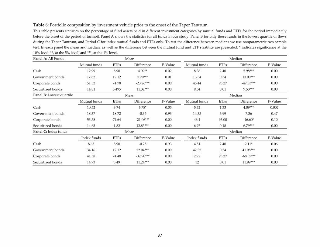
Table 6: Portfolio composition by investment vehicle prior to the onset of the Taper Tantrum

Panel A: All Funds

Mutual funds ETFs Difference P‐Value Mutual funds ETFs Difference P‐Value

Cash 12.99 8.90 4.09** 0.02 8.38 2.40 5.98*** 0.00

Government bonds 17.82 12.12 5.70*** 0.01 13.34 0.34 13.00*** 0.00

Corporate bonds 51.52 74.78 ‐23.26*** 0.00 45.44 93.27 ‐47.83*** 0.00

Securitized bonds 14.81 3.495 11.32*** 0.00 9.54 0.01 9.53*** 0.00

Panel B: Lowest quartile

Mutual funds ETFs Difference P‐Value Mutual funds ETFs Difference P‐Value

Cash 10.52 3.74 6.78* 0.05 5.42 1.33 4.09*** 0.002

Government bonds 18.37 18.72 ‐0.35 0.93 14.35 6.99 7.36 0.47

Corporate bonds 53.58 74.64 ‐21.06*** 0.00 46.4 93.00 ‐46.60* 0.10

Securitized bonds 14.65 1.82 12.83*** 0.00 6.97 0.18 6.79*** 0.00

Panel C: Index funds

Index funds ETFs Difference P‐Value Index funds ETFs Difference P‐Value

Cash 8.65 8.90 ‐0.25 0.93 4.51 2.40 2.11* 0.06

Government bonds 34.16 12.12 22.04*** 0.00 42.32 0.34 41.98*** 0.00

Corporate bonds 41.58 74.48 ‐32.90*** 0.00 25.2 93.27 ‐68.07*** 0.00

Securitized bonds 14.73 3.49 11.24*** 0.00 12 0.01 11.99*** 0.00

Mean Median

This table presents statistics on the percentage of fund assets held in different investment categories by mutual funds and ETFs for the period immediately

before the onset of the period of turmoil. Panel A shows the statistics for all funds in our study, Panel B for only those funds in the lowest quartile of flows

during the Taper Tantrum, and Period C for index mutual funds and ETFs only. To test the difference between medians we use nonparametric two‐sample

test. In each panel the mean and median, as well as the difference between the mutual fund and ETF stastitics are presented. * indicates significance at the

10% level; **, at the 5% level; and ***, at the 1% level.

Mean Median

Mean Median

37

Table 7: ETF summary statistics based on Taper Tantrum arbitrage exposure

Taper Tantrum

Credit 

Quality

Effecive 

DurationIO (%)

12 Month 

Flow Vol

Bid Ask 

SpreadLog(AUM) CRI (%) CRI (%)

High Arbitrage Exposure 2.76 5.52 47.55 7.78 0.004 4.64 3.300 1.7

Low Arbitrage Exposure 2.82 3.58 43.98 8.52 0.001 5.46 4.100 3.9

Difference ‐0.06 1.94 3.57 ‐0.73 0.003 ‐0.82 ‐0.800 ‐2.2

T‐stat ‐0.19 2.71*** 0.58 ‐0.41 2.80*** ‐1.73* ‐0.74 ‐2.48**

Pre‐Taper Tantrum

This table presents statistics on ETFs based on the average arbitrage opportunity during the months of the Taper Tantrum, June, July, and August

of 2013. For all corporate bond ETFs, we compute the monthly deviation as the average daily percentage difference between the ETF market

price and its NAV. We then split the ETFs into two groups based on this measure. ETFs with below median deviations trade at signficant discounts

during the turmoil episode and are deemed High Arbitrage Exposure . ETFs with average Tantrum deviation above the median are called Low Arbitrage Exposure . Here we test the significance of the differences in means between the mean credit rating and effective duration of the fund's

holdings from the holdings report and the portion of ETF shares outstanding held by insitutional investors, IO, prior to the onset of the event. We

also compute the volatiltiy of fund flows over the prior twelve months and compare the difference in the average monthly bid‐ask spread and

Turnover of the ETF betwen January and April 2013. We use the creation and redemption intensity measure of Da and Shive (2014) to create a

proxy for the level of arbitrage conducted by Authorized Participants, CRI . The proxy is computed as the standard deviation of ETF shares

outstanding in a month divided by the average shares of the ETF outstanding that month. Pre‐Taper Tantrum CRI is computed as the monthly

average between January and April and again during the Taper Tantrum.

38

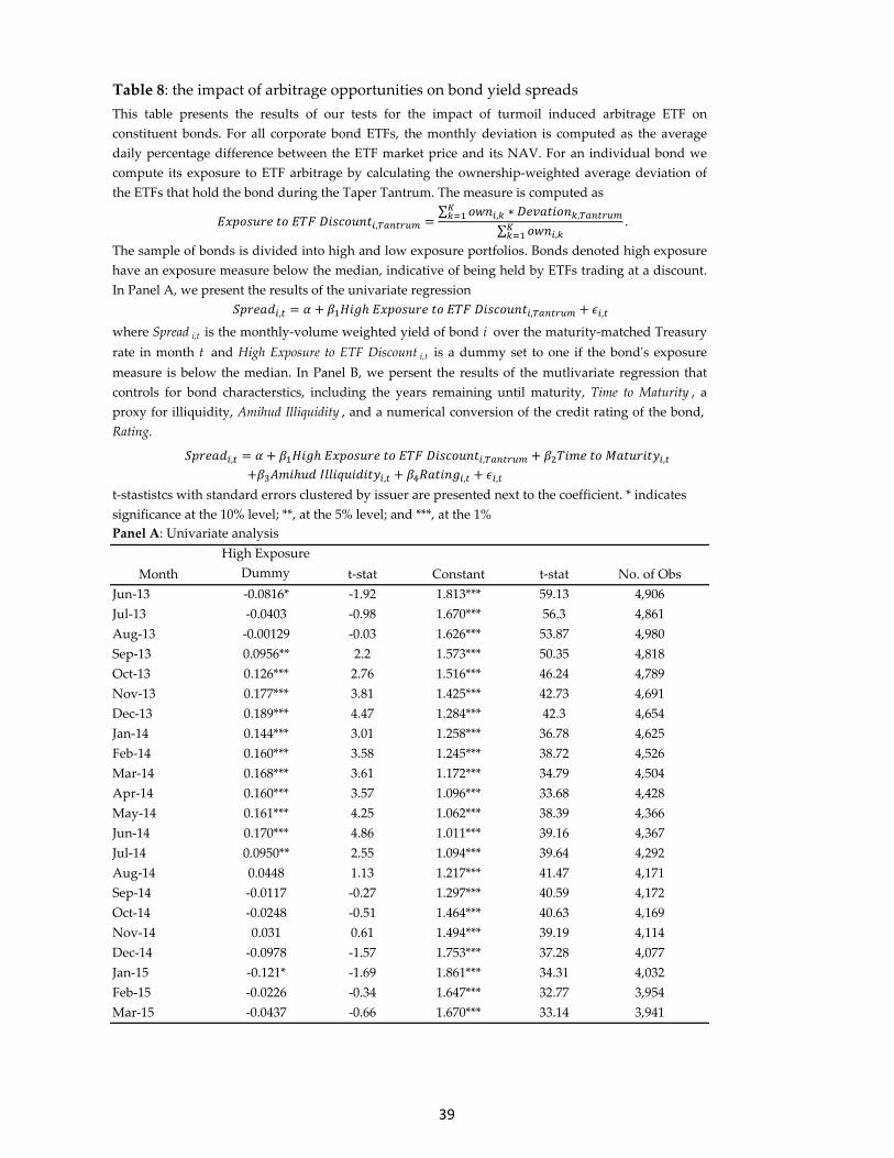
Table 8: the impact of arbitrage opportunities on bond yield spreads

Panel A: Univariate analysis

Month

High Exposure 

Dummy t‐stat Constant t‐stat No. of Obs

Jun‐13 ‐0.0816* ‐1.92 1.813*** 59.13 4,906

Jul‐13 ‐0.0403 ‐0.98 1.670*** 56.3 4,861

Aug‐13 ‐0.00129 ‐0.03 1.626*** 53.87 4,980

Sep‐13 0.0956** 2.2 1.573*** 50.35 4,818

Oct‐13 0.126*** 2.76 1.516*** 46.24 4,789

Nov‐13 0.177*** 3.81 1.425*** 42.73 4,691

Dec‐13 0.189*** 4.47 1.284*** 42.3 4,654

Jan‐14 0.144*** 3.01 1.258*** 36.78 4,625

Feb‐14 0.160*** 3.58 1.245*** 38.72 4,526

Mar‐14 0.168*** 3.61 1.172*** 34.79 4,504

Apr‐14 0.160*** 3.57 1.096*** 33.68 4,428

May‐14 0.161*** 4.25 1.062*** 38.39 4,366

Jun‐14 0.170*** 4.86 1.011*** 39.16 4,367

Jul‐14 0.0950** 2.55 1.094*** 39.64 4,292

Aug‐14 0.0448 1.13 1.217*** 41.47 4,171

Sep‐14 ‐0.0117 ‐0.27 1.297*** 40.59 4,172

Oct‐14 ‐0.0248 ‐0.51 1.464*** 40.63 4,169

Nov‐14 0.031 0.61 1.494*** 39.19 4,114

Dec‐14 ‐0.0978 ‐1.57 1.753*** 37.28 4,077

Jan‐15 ‐0.121* ‐1.69 1.861*** 34.31 4,032

Feb‐15 ‐0.0226 ‐0.34 1.647*** 32.77 3,954

Mar‐15 ‐0.0437 ‐0.66 1.670*** 33.14 3,941

This table presents the results of our tests for the impact of turmoil induced arbitrage ETF on

constituent bonds. For all corporate bond ETFs, the monthly deviation is computed as the average

daily percentage difference between the ETF market price and its NAV. For an individual bond we

compute its exposure to ETF arbitrage by calculating the ownership‐weighted average deviation of

the ETFs that hold the bond during the Taper Tantrum. The measure is computed as

The sample of bonds is divided into high and low exposure portfolios. Bonds denoted high exposure

have an exposure measure below the median, indicative of being held by ETFs trading at a discount.

In Panel A, we present the results of the univariate regression

where Spread i,t is the monthly‐volume weighted yield of bond i over the maturity‐matched Treasury

rate in month t and High Exposure to ETF Discount i,t is a dummy set to one if the bondʹs exposure

measure is below the median. In Panel B, we persent the results of the mutlivariate regression that

controls for bond characterstics, including the years remaining until maturity, Time to Maturity , a

proxy for illiquidity, Amihud Illiquidity , and a numerical conversion of the credit rating of the bond,

Rating.

t‐stastistcs with standard errors clustered by issuer are presented next to the coefficient. * indicates 

significance at the 10% level; **, at the 5% level; and ***, at the 1% 

, , ,

,∑ , ∗ ,

∑ ,.

, , ,

, , ,

39

Panel B: Multivariate analysis

Month

High Exposure 

Dummy t‐stat

Time to 

Maturity t‐stat

Amihud 

Illiquidity t‐stat Rating t‐stat Constant t‐stat No. of Obs

Jun‐13 0.0472 1.14 0.0105*** 4.71 13.44*** 10.31 0.210*** 55.01 ‐0.280*** ‐6.28 4,530

Jul‐13 0.0677 1.57 0.00912*** 3.88 11.37*** 8.64 0.185*** 47.87 ‐0.165*** ‐3.64 4,440

Aug‐13 0.014 0.3 0.0170*** 6.53 11.26*** 8.76 0.175*** 42.8 ‐0.142*** ‐2.94 4,453

Sep‐13 0.142*** 3.01 0.0127*** 4.94 13.85*** 9.18 0.178*** 41.41 ‐0.209*** ‐4.18 4,423

Oct‐13 0.167*** 3.31 0.0150*** 5.46 14.81*** 7.8 0.189*** 39.7 ‐0.354*** ‐6.52 4,356

Nov‐13 0.237*** 4.47 0.0118*** 4.12 11.28*** 6.63 0.184*** 36.71 ‐0.369*** ‐6.48 4,175

Dec‐13 0.249*** 5.24 0.0128*** 5.03 10.22*** 6.69 0.170*** 38.17 ‐0.401*** ‐7.92 4,181

Jan‐14 0.193*** 3.48 0.0157*** 5.15 14.43*** 7.32 0.175*** 33.96 ‐0.488*** ‐8.27 4,196

Feb‐14 0.182*** 3.57 0.0188*** 6.84 10.10*** 5.99 0.184*** 37.94 ‐0.550*** ‐10.06 4,044

Mar‐14 0.169*** 3.1 0.0215*** 6.99 10.31*** 6.32 0.171*** 32.81 ‐0.531*** ‐8.99 4,074

Apr‐14 0.152*** 2.96 0.0175*** 6.27 12.29*** 6.86 0.163*** 32.39 ‐0.510*** ‐9.06 4,023

May‐14 0.117*** 2.74 0.0190*** 8.29 10.59*** 7.24 0.141*** 33.42 ‐0.342*** ‐7.25 3,924

Jun‐14 0.112*** 2.84 0.0191*** 9.19 8.459*** 6.05 0.136*** 33.87 ‐0.326*** ‐7.38 3,919

Jul‐14 0.00539 0.13 0.0237*** 10.27 8.863*** 6.06 0.145*** 34.07 ‐0.343*** ‐7.25 3,812

Aug‐14 ‐0.0389 ‐0.88 0.0305*** 12.1 6.984*** 5.06 0.187*** 40.56 ‐0.606*** ‐12.03 3,604

Sep‐14 ‐0.0464 ‐0.97 0.0229*** 8.96 13.67*** 7.77 0.189*** 37.56 ‐0.536*** ‐9.86 3,695

Oct‐14 ‐0.0354 ‐0.69 0.0198*** 7.09 19.40*** 9.82 0.230*** 40.54 ‐0.712*** ‐11.92 3,734

Nov‐14 0.0418 0.74 0.0152*** 5.05 12.88*** 7.08 0.224*** 36.03 ‐0.585*** ‐8.97 3,645

Dec‐14 ‐0.155** ‐2.33 0.0250*** 7.06 20.01*** 10.97 0.292*** 39.46 ‐0.998*** ‐12.73 3,656

Jan‐15 ‐0.103 ‐1.31 0.0216*** 5.05 12.25*** 5.43 0.305*** 34.9 ‐0.959*** ‐10.33 3,632

Feb‐15 ‐0.0525 ‐0.72 0.0290*** 7.17 11.01*** 5.6 0.282*** 34.41 ‐0.991*** ‐11.41 3,523

Mar‐15 ‐0.0435 ‐0.61 0.0238*** 6.36 14.84*** 7.01 0.270*** 33.88 ‐0.872*** ‐10.18 3,568

 

40