Fe

dera

l Res

erve

Ban

k of

Chi

cago

The Term Structure and Inflation Uncertainty

Tomas Breach, Stefania D’Amico, and Athanasios Orphanides

December 2016

WP 2016-22

The Term Structure and Inflation Uncertainty

Tomas Breach, Stefania D’Amico, and Athanasios Orphanides∗

December 12, 2016

Abstract

This paper develops and estimates a Quadratic-Gaussian model of the U.S.term structure that can accommodate the rich dynamics of inflation risk pre-mia over the 1983-2013 period by allowing for time-varying market prices ofinflation risk and incorporating survey information on inflation uncertainty inthe estimation. The model captures changes in premia over very diverse pe-riods, from the inflation scare episodes of the 1980s, when perceived inflationuncertainty was high, to the more recent episodes of negative premia, whenperceived inflation uncertainty has been considerably smaller. A decomposi-tion of the nominal ten-year yield suggests a decline in the estimated inflationrisk premium of 1.7 percentage points from the early 1980s to mid-1990s. Sub-sequently, its predicted value has fluctuated around zero and turned negativeat times, reaching its lowest values (about -0.6 percentage points) before thelatest financial crisis, in 2005-2007, and during the subsequent weak recovery,in 2010-2012. The model’s ability to generate sensible estimates of the infla-tion risk premium has important implications for the other components of thenominal yield: expected real rates, expected inflation, and real risk premia.

Keywords: Quadratic-Gaussian Term Structure Models, Inflation Risk Premium,Survey Forecasts, Hidden Factors.

JEL Classification: G12, E43, E44, C58

∗Breach: Federal Reserve Bank of Chicago. E-mail: tbreach@frbchi.org. D’Amico: FederalReserve Bank of Chicago. E-mail: sdamico@frbchi.org. Orphanides: MIT Sloan School of Man-agement. E-mail: athanasios.orphanides@mit.edu. For helpful comments, discussions, and sugges-tions we thank Bob Barsky, Alejandro Justiniano, Don Kim, Thomas King, Anna Paulson, HiroTanaka, Min Wei, and seminar participants at the Federal Reserve Board and the Federal ReserveBank of Chicago. The views expressed here do not reflect offi cial positions of the Federal Reserve.

1

1 Introduction

Longer-term nominal yields contain rich information about real interest rates andinflation rates that market participants expect to prevail in the future. Extractingthis valuable information, however, is complicated by the presence of unobservableinflation risk premia (IRP) and real risk premia (RRP) that are widely acknowledgedto vary over time.Monetary policymakers are keenly interested in understanding these premia for

multiple reasons. The IRP embedded in nominal yields may reflect factors suchas uncertainty about inflation and the credibility of the monetary authority (e.g.,Argov et al. 2007; Palomino, 2012; Du et al., 2016), which may evolve over timewith the ability of the central bank to successfully communicate its policy strategyand deliver on its inflation objective. Changes in perceptions of inflation risks, suchas the inflation scare episodes of the 1980s (Goodfriend, 1993) or the risk of defla-tion following the last financial crisis (Kitsul and Wright, 2013), may cause abruptchanges in long-term yields not necessarily associated with shifts in expectations offuture interest rates or inflation. At times, significant changes in risk premia maycomplicate the transmission of monetary policy to longer-term rates, particularlywhen premia move in the direction opposite to expectations of short-term rates, ashas apparently been the case in the "conundrum" period (2004-06) and the "tapertantrum" episode (May-June 2013). Understanding inflation uncertainty and asso-ciated risk premia is important for the appropriate risk management of monetarypolicy. (Evans et al, 2015; and Feldman et al, 2016).In recent years, a new generation of dynamic term structure models has been

developed to estimate the various components of the term structure by allowingflexible specifications of risk premia while maintaining analytical tractability (e.g.,Dai and Singleton, 2000; Duffee, 2002). Despite considerable progress in modellingthe term structure, estimation of the IRP has proven challenging. Alternative spec-ifications estimated over different periods have resulted in a broad range of results(surveyed in Bekaert and Wong, 2010). Term structure models estimated using dataprior to the last financial crisis (e.g., Ang, Bekaert, and Wei, 2008; Buraschi andJiltsov, 2005; and Chernov and Mueller, 2012) report estimates of the IRP thatare larger in magnitude and mainly positive. In contrast, models focusing on morerecent data (e.g., Abrahams et al, 2013; Grishchenko and Huang, 2013; and Fleck-enstein, Longstaff, and Lustig, 2014), deliver values of the IRP that are smaller inmagnitude and often negative, especially at shorter maturities.One factor that could explain fluctuations in the IRP over time is the variation in

the level of actual and perceived inflation uncertainty. Inflation uncertainty makesnominal bonds risky, as their real value is eroded by surprise inflation, and thusis expected to affect the associated risk premium. Although the specific channelsmay differ, a relation between inflation uncertainty and the IRP emerges in numer-ous models, as highlighted for example in the survey by Gurkaynak and Wright

2

(2012). In the data, both actual inflation volatility and survey-based inflation un-certainty have declined notably since the 1980s (D’Amico and Orphanides, 2008), asthe Federal Reserve adopted policies that gradually reestablished its credibility tokeep inflation low and stable, following a period of monetary neglect. And as shownby D’Amico and Orphanides (2014), real-time measures of perceived inflation un-certainty contain meaningful information about future nominal bond excess returnsthat is not contained in current yields or forward spreads. Another potentially criti-cal factor for the evolution of the IRP is the changing covariance between bond andstock returns, which affects the hedging characteristics of Treasury nominal bonds.As indicated in Campbell, Sunderam, and Viceira (2016), for example, the stock-bond covariance was high and positive in the early 1980s but became negative inthe 2000s, which in their model mainly reflects time-variation in inflation volatilityand in the covariance between inflation and the real economy, with both accountingfor significant changes in the sign and size of nominal bond risk premia.We develop a Quadratic-Gaussian term structure model that is flexible enough

to encompass very diverse dynamic behaviors of the IRP over extreme episodeslike the early 1980s, characterized by high actual and expected inflation as well ashigh inflation uncertainty, and the post-2008 period, characterized by low inflation(and mild deflation) as well as very low expected inflation and inflation uncertainty.The richer dynamic of the IRP is achieved by having time-varying market prices ofinflation risk in the model, which translates into time-varying inflation volatility andtime-varying covariances between yield curve factors and inflation. To obtain reliableestimates of the parameters governing these sources of inflation risk and the IRP, weincorporate information from survey-based inflation uncertainty in the estimation.Using this new data input, which captures real-time perceptions of inflation risk,proves quite valuable for pinning down the dynamics of the IRP which, in turn,has important implications for the other components of nominal yields: expectedreal short-term rates, expected inflation, and the RRP. The key novelty of thisapproach is to tackle the diffi culties in the estimation of the IRP by allowing forvery flexible market prices of inflation risk and by using a real-time measure ofinflation uncertainty.Introducing survey-based information about second moments may also be seen as

an extension of the approach developed in Kim and Orphanides (2012) and Chernovand Mueller (2012) who augment term structure models with information fromsurvey first moments. Similarly to the first of these studies, we include surveyforecasts of short-term interest rates to guard against estimation imprecision andbias due to the highly persistent nature of interest rates; and, similarly to the secondstudy, we include survey forecasts of inflation that help pin down expected inflationand real rates over a long sample period for which TIPS yields are not available.To account for the possibility that survey forecasts provide noisy information and

to let the data determine the extent of this noise, following Kim and Orphanides(2012) we allow for unconstrained variances of the measurement errors around all

3

forecasts in the estimation. Acknowledging the presence of measurement errors isparticularly important for survey-based inflation uncertainty, which is an imputedvariable derived from the subjective probability distributions in the Survey of Profes-sional Forecasters (SPF) using the methodology in D’Amico and Orphanides (2008).In addition, following the intuition in Duffee (2011) and motivated by preliminary

regressions similar to those conducted by Joslin, Priebsch, and Singleton (2014), inour model inflation-related variables are not fully spanned by the current nominalyield curve. This is achieved through two modelling choices. First, we introduce ashock capturing short-run variations in CPI inflation that do not require a monetary-policy response, such as, short-lived changes in energy and food prices. Second,one of the factors is hidden in the nominal yield curve and can only influence thefirst and second moments of inflation. In principle, both of these features can beimportant because, while the conditional volatility of the Brownian shock specificto CPI affects inflation uncertainty and risk premia but not the forecast of inflation(i.e., its expected value is zero), the hidden factor can influence expected inflation.Moreover, the conditional volatility of the innovations to the hidden factor can alsocontribute to fluctuations in inflation uncertainty and risk premia.The resulting model produces IRP estimates at the 10-year horizon that are

larger and positive in the 1980s, then decline by about 1.7 percentage points bythe mid 1990s, and subsequently become negative at times, for example during theconundrum period (2005-07) and during the deflation scare of 2010-2012. The es-timates also capture episodes of sharp increases in the IRP, as for instance duringthe taper tantrum of May-June 2013. Further, despite being estimated withoutthe use of TIPS yields, the model generates real yields that closely resemble thoseon TIPS, except for a residual very similar to the liquidity premium estimated inD’Amico, Kim, and Wei (2016). The model also does a good job at fitting thesurvey-based one-year expected inflation and inflation uncertainty, and it producesexpected short-term rates that closely match those from survey forecasts. Withregard to longer-term trends, the model captures the decline in long-term infla-tion expectations from the 1980s to the 2000s that is associated with the FederalReserve’s overall disinflationary policies over this period as well as the decline inlong-term expectations of the short-term real interest rate reflecting the decline inthe equilibrium real interest rate.The rest of the paper is organized as follows. Section 2 sets up the Quadratic-

Gaussian model. Section 3 compares our model to other key studies in the literature.Section 4 presents the state-space form of the model and the data. Section 5 providesdetails about the identification and estimation methodology. Section 6 presentsthe main model’s empirical results and comparisons with alternative specifications,which help assess the contribution of key elements to its improved performance.Section 7 offers concluding remarks.

4

2 A Quadratic Gaussian Model

In this section we develop a Quadratic Gaussian model of the term structure of inter-est rates that accommodates nominal yields, CPI inflation, survey-based expectedinflation, expected interest rates, and inflation volatility.

2.1 The basic building blocks

We start with specifying the state factor dynamics under the physical measure, P:

[dxtdzt

]=

[κx2×2 02×101×2 κz1×1

] [(µx − xt)2×1(µz − zt)1×1

]dt+

[Σx2×2 02×1σx,z σz

] [dBx

t

dBzt

]where zt is a factor hidden in the nominal yield curve in the sense of Duffee (2011)but its shocks can be correlated with shocks relevant for nominal interest rates asindicated by the unconstrained σx,z, Bt denotes a 3-dimensional standard Brownianmotion, and thus all the factors are Gaussian.The nominal pricing kernel under P is given by:

dMNt

MNt

= −rNt dt− λNt ′dBxt

where the nominal short rate is an affi ne function of only two state variables:

rNt = ρN0 + ρN ′1 xt,

and the 2-dimensional vector of the market price of nominal risk is given by:

λNt = λN0 + ΛNxt,

with ΛN being a 2 × 2 constant matrix that will be left unrestricted to allow for aflexible specification of the market price of nominal risk. However, by preventing λNtand rNt from loading on zt, we make sure that this factor is unspanned by nominalyields.1

The log price level follows the process

d logQt = πtdt+ λq′t dBx∗

t + ωtdB⊥t

and is governed by x∗t = [xt, zt] rather than xt, as the factors underlying the nominalyields are not suffi cient to span inflation and expected inflation, which is affi ne inx∗t :

πt = ρπ0 + ρπ′1 x∗t ,

1This can be also achieved by imposing restrictions under the risk-neutral measure as in Duffee(2011), and we verified that results are not very sensitive to the way we impose the unspanningrestrictions.

5

and the two conditional volatility processes are given by

λqt = λq0 + Λqx∗t ,

ωt = ω0 + ω′1x∗t ,

where ρπ0 and ω0 are scalars, ρπ1 and λ

q0 are 3 × 1 vectors, ω′1 is a 1 × 3 vector, Λq

is a 3× 3 matrix, and dBx∗t dB

⊥t = 0. The orthogonal shock specific to the inflation

process is supposed to capture, for instance, short-run variations in inflation thatdo not require a monetary-policy response and thus do not affect the nominal shortrate (Kim, 2008). In particular, since we use total CPI in our estimation, not only itis important to have a separate shock for CPI innovations driven by changes in foodand energy prices, but since these components are usually more volatile it is keyto allow for time variation in the conditional volatility of this shock. Overall, thisimplies that we treat much of high-frequency variation in inflation as unspanned byinterest rates.The real pricing kernel is given by MR

t = MNt Qt, which by Ito’s Lemma follows

the dynamics:

dMRt

MRt

=dMN

t

MNt

+dQt

Qt

+dMN

t

MNt

dQt

Qt

= −rRt dt− λR′t dBx∗

t − ωtdB⊥t

where the real short rate becomes a quadratic function of the state variables becauseof the interaction term dMN

t

MNt

dQtQt, as each of these elements contains a state-dependent

market price of risk, that is, λN(xt) and λq(x∗t ), respectively:

rRt = ρR0 + ρR′1 x∗t + x∗′t ΨRx∗t ,

all parameters are linked by the no-arbitrage conditions:

ρR0 = ρN0 − ρπ0 + λN ′0 λq0 −

1

2(λq′0 λ

q0 + ω20)

ρR1 = ρN1 − ρπ1 + Λq′λN0 + ΛN ′λq0 − Λq′λq0 − ω0ω1λRt = λNt − λ

qt

ΨR = ΛN ′Λq − 1

2Λq′Λq − 1

2ω1ω

′1.

2.2 Bond Pricing

Under the risk-neutral measure, Q, x∗t follows the dynamics:

dx∗t = κ (µ− x∗t ) dt+ Σ(dBx∗

t + λitdt− λitdt)

=(κµ− κx∗t − Σλi0 − ΣΛix∗t

)dt+ Σ

(dBx∗

t + λitdt)

= κ (µ− x∗t ) dt+ ΣdBλt

6

where

κ = κ+ ΣΛi

κµ = κµ− Σλi0

dBλt = dBx∗

t + λitdt

and i = N,R indicating either the nominal or real risk neutral measure.The price of a nominal and real zero-coupon bond with maturity τ is:

P it,τ =

Et(Mit+τ )

M it

= EQt

(exp

(−t+τ∫t

risds

))= exp

[Aiτ +Bi′

τ xt + x′tCiτxt], i = N,R

with the solution satisfying the following differential equations:

dAiτdτ

= −ρi0 +Bi′τ κµ+

1

2Bi′τ ΣΣ′Bi

τ + tr[Σ′Ci

τΣ]

dBiτ

dτ= −ρi1 − κ′Bi

τ + 2Ciτ κµ+ 2Ci

τΣΣ′Biτ

dCiτ

dτ= −Ψi − Ci

τ κ− κ′Ciτ + 2Ci

τΣΣ′Ci′τ .

In the case of nominal bonds (i.e., i = N), CNτ = 0, as in this model we start with

specifying an affi ne nominal short rate and the real short rate inherits the quadraticcomponent through the no arbitrage conditionMR

t = MNt Qt, and therefore nominal

bonds’prices preserve the same functional form usually obtained in affi ne Gaussianmodels. It follows that since yit,τ = − 1

τlog(P i

t,τ ), nominal and real yields are equalto:

yNt,τ = aNτ + bN ′τ xt

yRt,τ = aRτ + bR′τ x∗t + x∗′t c

Rτ x∗t ,

where aiτ = − 1τAiτ , b

iτ = − 1

τBiτ , and c

iτ = − 1

τCiτ .

2.3 Inflation: Expected and Unexpected

Inflation between t and t+ τ is defined as:

it,τ ,1

τlog

Qt+τ

Qt

=1

τ

[∫ τ

0

π(x∗t+s)ds+

∫ τ

0

λq(x∗t+s)′dBx∗

s +

∫ τ

0

ω(x∗t+s)′dB⊥s

]and annual average expected inflation over horizon τ is given by:

7

Et [it+τ ] =1

τ

∫ τ

0

Et [πt+s] ds

therefore unexpected inflation can be expressed as follows:

it,τ − Et [it+τ ] =1

τ

∫ τ

0

(πt+s − Et [πt+s]) ds+

+1

τ

[∫ τ

0

(λq0 + Λqx∗t+s

)′dBx∗

s +

∫ τ

0

(ω0 + ω1x

∗t+s

)′dB⊥s

]=

= ρπ′1

∫ τ

0

ξsds+ (x∗t − µ)′[∫ τ

0

e−κs′Λq′dBx∗

s +

∫ τ

0

e−κs′ω1dB

⊥s

]+

(λq0 + Λqµ)′∫ τ

0

dBx∗

s + (ω0 + ω′1µ)′∫ τ

0

dB⊥s +

∫ τ

0

ξ′sΛq′dBx∗

s +

∫ τ

0

ξ′sω1dB⊥s .

It is easy to note that for the unexpected inflation to be time varying, that is, to befunction of the factors x∗t , it is suffi cient that either Λq or ω1 are different from zero,meaning that the time-varying market prices of inflation risk are the key features ofthe model permitting time variation in inflation volatility, which we derive below.We can re-write the unexpected inflation in matrix form:

it,τ − Et [it+τ ] =1

τ(C +Dx∗t )

′ ζτ

C =

ρπ′1λq0 + Λqµ−µ1

ω0 + ω′1µ−µ1

, D =

03×303×3I3×301×301×3I3×301×3

, ζτ =

∫ τ0ξsds∫ τ

0dBx∗

s∫ τ0e−κs

′Λq′dBx∗

s∫ τ0ξ′sΛ

q′dBx∗s∫ τ

0dB⊥s∫ τ

0e−κs

′ω1dB

⊥s∫ τ

0ξ′sω1dB

⊥s

where

∫ τ0ξsds = κ−1

∫ τ0

(I3×3 − e−κs

′)ΣdBx∗

s . By observing the elements in ζτ ,it is easy to note that the unexpected inflation is driven by all four shocks in themodel: the innovations to the yield factors, the innovations to the hidden factor,and the shock specific to CPI, as well as the conditional volatility of these shocks.The inflation variance is a quadratic function of the state variables:

var(it,τ ) =1

τ 2Et[(C +Dx∗t )

′ ζτζ′τ (C +Dx∗t )

].

8

In the Appendix A, we provide a detailed derivation of all the elements in ζτζ′τ , the

block matrix whose expected value delivers the variances of and covariances betweenthe shocks that drive unexpected inflation (and thus uncertainty).As it will become clear later, having a survey-based measure of inflation uncer-

tainty allows us to better pin down some of the parameters in C and ζτ . Moreimportantly, the vector of parameters ω1 can be identified only if we incorporatesurvey data on this second moment.

2.4 Inflation Risk Premium

We now turn to the main object of interest in this study, that is, the IRP, which isdefined as follows:

IRPt = rNt − rRt − πt = −(λN ′0 λ

q0 +

1

2λq′0 λ

q0 −

1

2ω20

)+

−(Λq′λN0 + ΛN ′λq0 − Λq′λq0 − ω0ω1

)′x∗t +

−x∗′t(

ΛN ′Λq − 1

2Λq′Λq − 1

2ω1ω

′1

)x∗t .

Our IRP has a richer dynamic behavior than permitted by previous studies in theliterature, for example, Chernov and Mueller (2012) and D’Amico, Kim and Wei(2016), who already allowed for quite flexible dynamics. Particularly, in D’Amico,Kim and Wei (2016), the IRP is linear in the state variables and is time varyingbecause of the state-dependent market price of nominal risk—i.e., the time variationis obtained by having just the term ΛN ′λq0 different from zero in the expressionabove.In this model, the resulting specification of the IRP has two additional sources

of flexibility. First, as shown in the last term of the above equation, it is a quadraticfunction of the state variables because of Λq and ω1. Second, the linear portion canvary because either the market price of nominal risk or the market price of inflationrisk changes over time, as ΛN , Λq, and ω1 multiply x∗t .This extremely adaptable functional form should allow our model to accommo-

date very different dynamic behaviors of the IRP over a long and diverse sampleperiod including the inflation scare episodes of the 1980s when, in principle, percep-tions of heightened inflation risk would have commanded large and positive valuesof the IRP, and the deflation scare episode of 2009-2012, when disinflation and lowgrowth made nominal bonds a very good hedge against adverse outcomes possiblypushing the IRP into negative territory.To provide a simple intuition for why the data on real-time inflation variance

can improve the estimation of the IRP, we rewrite the IRP in the following way:

9

IPRt,τ = −1

τlog

1 +Cov

(MRt+τ

MRt, QtQt+τ

)Et

(MRt+τ

MRt

)Et

(QtQt+τ

)+ Jt,τ

≈ −1

τlog[1 + Cov

(rRt,τ , it,τ

)/Et

(rRt,τ)Et (it,τ )

]= −1

τlog[1 +

(Cov

(rNt,τ , it,τ

)− var(it,τ )

)/Et

(rRt,τ)Et (it,τ )

].

where for simplicity we are assuming that the real pricing kernel is mainly drivenby the real yield and we are ignoring the Jensen’s inequality term, which in practiceis fairly small.2

Based on this simplification, it is easy to see that to the extent that variationsin the covariance between the real economy and inflation arises from fluctuations inthe variance of inflation, accurate measurement of these specific fluctuations wouldbe important. Survey data on real-time inflation uncertainty serve this purpose,that is, they help identifying fluctuations in the variance of inflation and thus inthe time-varying IRP. Further, as we will explain shortly in Section 4.1 where wedescribe the covariances of the state variables, having a time-varying market priceon inflation risk λqt also allows time variation in the covariance between nominalinterest rates and inflation, thus having more data to pin down λqt also helps in theestimation of that covariance.

3 Comparison to previous studies

This paper draws on contributions from several streams of the term-structural lit-erature. First of all, to achieve time-varying second moments, we favor the useof Quadratic Gaussian (QG) models because affi ne term-structure models with sto-chastic volatility typically fail to produce reasonable risk premia (Dai and Singleton,2002 and Duffee, 2002) and fitted yield volatilities that resemble the time-varyingvolatilities estimated from semi-parametric time-series models (Ahn, Dittmar, andGallant, 2002; Collin-Dufresne, Goldstein, and Jones, 2009). For example, Haubrich,Pennacchi, and Ritchken (2012) develop a completely affi ne model that has four sto-chastic drivers and seven factors, but it still generates IRP that do not seem verysensible up to the two-year horizon, as it is mostly negative even in the early 1980s,when most other studies find that IRP estimates reach their highest peak.In contrast, as shown in Kim (2004), QG models do not seem to exhibit a trade-

off between fitting yield volatility and risk premia, therefore, we build on these typeof models (e.g., Kim, 2004; and Kim and Singleton, 2012) and expand on them

2Jt,τ ≡ −( 1τ )[log(Et(Qt/Qt,τ ))− Et(log(Qt/Qt,τ ))].

10

by adding flexibility to market prices of inflation risk and allowing for unspannedinflation risk. Particularly, we decided to expand in this direction because Le andSingleton (2013) show that substantial variation in risk premia is unspanned bynominal bond yields and seems to arise from a time-varying market price of inflationrisk; and, D’Amico and Orphanides (2014) show that perceived inflation risk is animportant driver of excess bond returns beyond and above the information containedin nominal yields.To allow for unspanned inflation risk, our model includes some of the unspan-

ning restrictions emphasized in Duffee (2011) and Joslin, Priebsch, and Singleton(2014), and similarly to the latter, we also run preliminary regressions to motivateour hidden factor. Table 1 reports the percentage of variation (R2) in inflation re-lated variables explained by the 3 latent factors of an affi ne term-structure modelestimated using only nominal yields and short-term rate forecasts. We find thatalthough more than 80% of variation in expected inflation is explained by thesefactors, only half of the variation in inflation uncertainty is explained by those samefactors. In line with this observation, our unspanning restrictions permit our thirdfactor to drive both expected inflation and inflation uncertainty while remaininghidden from the nominal yield curve.Our paper is also closely related to studies emphasizing the size and nature of

the IRP. For example, similarly to Chernov and Mueller (2012), we use survey-based inflation expectations at various horizons, but while their preferred modeluses TIPS yields in the estimation, we use short- and long-horizon survey forecastsof nominal interest rates that together with surveys forecasts of inflation help topin down the term-structure of expected real rates over a longer sample. A moreimportant difference is that in this paper, we focus on modeling time variation inthe market price of inflation risk and incorporate information from survey-basedinflation variance, which in turn permits us to identify a more flexible dynamic ofthe IRP. Another relevant study that, however, uses a quite different approach isBuraschi and Jiltsov (2005). Specifically, these authors develop a structural modelthat can identify the underlying nominal and real factors driving the IRP, but alsosuffers from the shortcoming that the market price of risk, even if state dependent,is not as flexible as ours, which is based on a more reduced-form approach. Further,their dataset consists only of interest rates, CPI, and money supply, and thus doesnot include any information from survey forecasts. In addition, differently from ourwork, in both of these studies, the sample period stops before 2008.Finally, our study is also related to equilibrium term-structure models implying

that time-variation in expected excess returns of nominal risk-free bonds is drivenby changes in variances of real and inflation risks (e.g., Bansal and Shaliastovich,2012); however, in most of these models, the market price of risk is assumed tobe constant and macro risk is fully spanned by nominal yields. This is also truefor Campbell, Sunderam, and Viceira (2016), who assume that all time variationin bond risk premia is driven by variation in bond risk and not by variation in the

11

aggregate price of risk. Importantly, their estimates of the variables governing bondrisk are informed by realized second moments of high-frequency returns, while ourestimates are informed by a real-time measure of perceived inflation risk. Moreover,we are more focused on modeling and estimating the IRP, while they emphasizethe importance of the time-varying stock-bond covariance for the term structure ofinterest rates.

4 State-space form and data

In this section, we first present the state equation and emphasize the role of time-varying market prices of inflation risk in generating time variation in the covariancesof the state variables, then we turn to the observation equations and highlight howthey link the data to our state variables.

4.1 State variables and their covariances

We rewrite the model in a state-space form and estimate it by quasi maximum like-lihood (QML) using the Augmented State Space Extended Kalman Filter methoddeveloped in Kim (2004). The basic idea of his approach is to augment the statevector st with the quadratic term vech(x∗tx

∗′t ), st = [x∗t , vech(x∗tx

∗′t ), qt]

′, such thatthe state equations can be written in the usual linear matrix form:

st = Gh + Γhst−h + ηst ,

where ηst = [Σηt, vt, λq(x∗t−h)

′ηt + ω(x∗t−h)′η⊥t ] is the vector of innovations to x∗t ,

vech(x∗tx∗′t ), and qt, respectively, and vt, Gh and Γh are defined in the Appendix B.

The conditional variance of the state variables, Ωst−h = V ar(st|It−h) = Et−h(η

stηst),

is given by:

E

Σηtη′tΣ′ Σηtv

′t Σηtη

′tλq(x∗t−h)

′

vtη′tΣ′ vtv

′t vtη

′tλq(x∗t−h)

′

λq(x∗t−h)ηtη′tΣ′ λq(x∗t−h)ηtv

′t λq(x∗t−h)ηtη

′tλq(x∗t−h)

′ + ω(x∗t−h)2η⊥2t

=

V art−h(x∗t ) Covt−h(x

∗t , vech(x∗tx

∗′t )) Covt−h(x

∗t , qt)

Covt−h(x∗t , vech(x∗tx

∗′t )) V art−h(vech(x∗tx

∗′t )) Covt−h(vech(x∗tx

∗′t ), qt)

Covt−h(x∗t , qt) Covt−h(vech(x∗tx

∗′t ), qt) V art−h(qt)

It is worth noting the different roles played by λq(x∗t ) and ω(x∗t ): λ

q(x∗t ) allowscovariances between all latent factors and the log price level qt to be time-varyingand also contributes to the time variation in the variance of qt; in contrast, ω(x∗t )governs only the variance of qt. This suggests that, in principle, the estimated valuesof ω(x∗t ) should be strongly influenced by data on inflation uncertainty, which willalso help identifying fluctuations in the variable λq(x∗t ).

12

4.2 Observation equations and data

From January 1983 to December 2013, we observe seven nominal yields Y Nt =

yNt,τ i7i=1, the 6-month, 12-month, and 6-to-11 years ahead forecasts of the nomi-

nal short rate f 6mt , f 12mt , and f longt respectively, the survey inflation expectationsat one- and 11-year horizons EI1yt and EI11yt , as well as the one-year real-timeinflation uncertainty IU1yt . We collect all the observable variables in the vectorot = [Y N

t , f6mt , f 12mt , f longt , EI1yt , EI

11yt , IU1yt ]′ and write also the observation equa-

tions in a matrix form:

ot = a+ Fst + εt

where εt denotes the vector of measurement errors, assumed to be i.i.d., with freelyestimated variances: εY

N

t,τ i∼ N(0, δ2N,τ i), ε

ft,τ i ∼ N(0, δ2f,τ i), ε

EIt,τ i∼ N(0, δ2EI,τ i), and

εIUt ∼ N(0, δ2IU).More details about the functional form of the observation equations and thus of

a and F are provided in Appendix C. However, we stress here how each observationequation links specific data to all or some of the state variables. Further, it shouldbe noted that inflation and survey-based variables are not available for all dates,which introduces missing data in the observation equation and are handled in thestandard way by allowing the dimensions of a and F to be time-dependent (see, forexample, Harvey 1989).The first seven measurement equations relate observable Treasury nominal yields

only to the two state variables xt, due to the unspanning restrictions. Specifically,we use the 3- and 6-month Treasury bill rates from the Federal Reserve Board’sH.15 release and converted them to continuously compounded basis. The 1-, 2-, 4-,7-, and 10-year nominal yields are based on zero-coupon yield curves fitted at theFederal Reserve Board (see Gurkaynak, Sack, and Wright, 2007; Gurkaynak, Sack,and Wright, 2010 for details). We sample yields at the weekly frequency and assumethat the monthly CPI-U data is observed on the last week of the current month.34

Similarly, our eighth and ninth measurement equations also link the 6- and 12-month-ahead forecasts of the 3-month Treasury bill rate from Blue Chip FinancialForecasts (BCFF), which are available monthly, only to xt. We complement thesemeasurement equations with another one that uses the long-range forecast (6-to-11years ahead) of the same rate. In BCFF, this forecast is provided only semiannually,but we follow the procedure in D’Amico and King (2015) to convert them to aconsistent quarterly frequency, as we think that information from longer-term surveyforecasts is very important to correctly estimate the persistency of the yield factorsunder the physical measure. The basic idea consists of combining the long-range

3Here we abstract from the real-time data issue by assuming that investors correctly infer thecurrent inflation rate in a timely fashion.

4The data source for the nominal yields and CPI-U is Haver.

13

forecasts from BCFF with those from Blue Chip Economic Indicators (BCEI). Thisis because BCFF provide these long-range projections in June and December, whilethe BCEI report them in March and October, these values can then be interpolatedto obtain the September value and have a regularly-spaced quarterly time series.5

The eleventh and twelfth equations relate the observed measures of expectedinflation at the 1- and 11-year horizon to all state variables x∗t , as inflation-relatedvariable are allowed to load on the hidden factor. Specifically, we use the medianforecast of average inflation over the following year from the Survey of ProfessionalForecasters (SPF) because it is reported at a consistent quarterly frequency andtherefore does not require interpolation. However, since the longest available fore-casting horizon in these data is one-year ahead, to measure longer-term inflationexpectations we turn again to the BCS, which has been providing semiannual long-range (2-to-6 and 7-to-11 years ahead) consensus forecasts of CPI since 1983. Oncewe have converted them to a consistent quarterly frequency using the same method-ology described for interest rate forecasts, we can compute the expected averagevalue over the next 11 years– by taking the weighted average of the one-year, 2-6-year, and 7-11-year expectations, respectively.Finally, the last observation equation relates the real-time measure of inflation

variance at one-year horizon to all state variables x∗t as well as to vech(x∗tx∗′t ). The

real-time measure of inflation variance is derived from the subjective probabilitydistributions in the SPF using the methodology of D’Amico and Orphanides (2008),therefore it should capture ex-ante inflation risk perceived by investors rather thanex-post realized volatility.

5 Identification and estimation methodology

Except for the unspanning restrictions already described in Section 2.1, for all otherparameters in the model, we only impose restrictions that are necessary for achievingidentification to allow a maximally flexible correlation structure between the factors,which has shown to be critical in fitting the rich behavior of risk premia observedin the data. In particular:

µ = 03×1, κ =

κ11 0 00 κ22 00 0 κ33

, Σ =

1 0 0Σ21 1 0Σ31 Σ32 1

and ΛN is unrestricted.Regarding the set of parameters that allow for time variation in the variance of

inflation and covariances of inflation with the other state variables, we have that Λq

is lower triangular and ω1 is left unrestricted:

5For more details see the Appendix in D’Amico and King (2015).

14

Λq =

Λq11 0 0

Λq21 Λq

22 0Λq31 Λq

32 Λq33

and ω1= [ω11 ω12 ω13]

This implies that the market price of inflation risk can be affected by all threefactors x∗t and their interactions, and that the conditional volatility of the shockspecific to CPI is also affected by the same three factors x∗t .To facilitate the estimation by starting with reasonable initial values of the pa-

rameters and to make the results easily replicable, we break the estimation in afew easier steps: We first perform a “pre”-estimation where a set of preliminaryparameter estimates governing the nominal term structure is obtained using Y N

t

and survey forecasts of 3-month TBill rate alone;6 second, based on these estimatesand data on Y N

t , we can obtain a preliminary estimate of the state variables, xtand dBt; third, a regression of monthly inflation onto estimates of xt and dBt givespreliminary estimates of ρπ0 , ρ

π1 , λ

q0, Λq, ω0; fourth, a regression of quarterly infla-

tion uncertainty on xt and x2t gives preliminary estimates of ω1; and finally, thesepreliminary estimates are used as starting values in the full, one-step estimation ofall model parameters by QML.

6 Empirical Findings

In this section, we first provide a summary description of the results based onour "full" model specification, which includes all the features described above andincorporates in the estimation all the information from surveys. Then, we dissectthe results to highlight the contribution of key elements of our approach separately,by presenting comparisons with simpler specifications and with the estimation thatdoes not make use of survey information on the second moment of inflation.

6.1 Full model specification

A visual description of our main findings is presented in Figures 1, 2, and 3. Specif-ically, Figure 1 shows the decomposition of the 10-year nominal yield into threecomponents: The real yield (including the RRP), the expected inflation at the per-tinent horizon, and the corresponding IRP. Figure 2 focuses on the four componentsof the 10-year nominal yield, as in addition to the expected inflation rate and IRP(also shown in Figure 1), it shows the expected future short real rate and the RRPseparately. Finally, Figure 3 summarizes the overall fit of the full model, as itcompares the model-implied one-year inflation variance, 5-year real yield, one-year

6It is important to keep in mind that in this preliminary estimation we do not impose unspanningand therefore derive 3 latent factors from the nominal term structure. This implies that especiallythe third factor will have a dynamic quite different from that one of the hidden factor obtained inthe final step of the estimation.

15

expected inflation, and one-year expectation of the nominal short-term rate to theircounterparts in the data (shown in orange).As it can be seen in Figure 1, the model estimation over the 1983 to 2013 period

captures the main characteristics of the time variations in longer-term nominal yieldsthat have been discussed in the earlier literature. Overall, inflation expectations, realinterest rate expectations, the IRP as well as the RRP all trended down during the1980s and 1990s. Real yields dominate the other components in accounting for thefluctuations in nominal yields. However, the major sources of variation differ at lowand high frequencies. While the expectation component of the yield– the expectedreal interest rate and expected inflation– dominate at business cycle frequencies,the risk premia largely drive higher-frequency fluctuations.Focusing on the estimates of the 10-year IRP in Figure 2, our findings suggest

that it was consistently positive in the first part of the sample, reaching its highestpeak (about 1.7 percentage points) in the spring of 1984, and then spiked again inMay-October 1987. Since the mid 1990s, it has fluctuated around zero, reaching itsmost negative values (about −0.6 percentage points) in 2005-2007, just before themost recent financial crisis, and during the subsequent weak recovery, in 2011-2012.The largest fluctuations in the estimated IRP capture notable episodes docu-

mented over this period that reflected changes in perceptions of inflation risks. Thespikes in 1984 and 1987, for example, coincide with the narrative of the inflationscares of the 1980s documented by Goodfriend (1993). Similarly, the substantialdecline over the 2010-2012 period largely coincides with the deflation scare episodedescribed in Kitsul and Wright (2013). Our estimates of the IRP also captureepisodes that have occupied discussions relating to monetary policy. One notableexample is the "conundrum" period in the mid-2000s when, as shown in Figure 2,risk premia started declining sharply in 2004 while the Federal Reserve was raisingshort-term nominal interest rates. Another example is the "taper-tantrum" in thesummer of 2013, when longer-term Treasury yields rose dramatically following FedChairman Ben Bernanke’s remarks about the possibility of moderating the pace ofasset purchases later that year, implying a lower degree of expected monetary policyaccommodation.Interestingly, our findings also illustrate the time-varying nature of the covariance

of yield components. While in much of the 1980s, all four components broadlymove in the same direction, after 1987 expectations and risk premia start movingin opposite directions. This pattern is particularly evident in 1987-1992, 2001-02,2004-08, and 2011-2013. These are periods highlighting the presence of a hiddenfactor: Changes in the hidden factor would move the IRP and RRP in the sameamount of but opposite to the expected future short real rates and the expectedinflation. This could explain the conundrum period and also indicates that theentire increase in the nominal yields observed during the taper tantrum was indeeddue to increases in risk premia.Turning attention to the expected inflation and expected short-term real interest

16

rates, Figure 2 also shows that the model captures their secular decline since the1980s. With respect to inflation expectations, this decline is consistent with theFederal Reserve’s successful disinflation efforts over the 1980s and 1990s and itsstrategy of maintaining mostly stable inflation since then. With respect to thedecline in long-term expectations of the short-term real interest rate, the model’sfindings are consistent with studies suggesting a notable decline in the equilibriumreal interest rate over this period (Holtson, Laubach and Williams, 2016).Moving to the overall fit of the full model, Figure 3 suggests that the model-

implied variables match their data counterparts quite well. Starting from the top leftpanel, it can be noted that the fluctuations in the model-implied one-year inflationvariance track quite closely those in the survey-based inflation variance. Further,despite being estimated without the use of TIPS yields, as shown in the top rightpanel, the full model generates a 5-year real yield that closely resembles that one onTIPS (when available), except for a residual very similar to the liquidity premiumestimated in D’Amico, Kim, and Wei (2016). In their study, the estimated TIPSliquidity premium is fairly high and positive in the early years of TIPS, then declinessteadily and stays close to zero from 2004 until the height of the 2007-08 financialcrisis, when it surges to its highest level, to then turn negative around 2011. Thetwo bottom panels indicate that the model can match pretty well one-year surveyforecasts of inflation and of the short-term rate. This also illustrates that the surveyinformation about first moments of key variables like inflation and the short ratehelp the model capturing the slow moving trend in those expectations as well as theZLB period.

6.2 Dissecting the model’s key features

The main empirical contributions of our study can be more easily illustrated andunderstood by comparing the empirical performance of the full model to the resultsderived from different model specifications, with each specification obtained by re-moving from the full model one of its key ingredients. We consider three simplifica-tions: 1) the model without time-varying inflation volatility, called Model No_TVV(No time-varying volatility, i.e., ω1 = 03×1 and Λq = 03×3); 2) the model estimatedwithout data on inflation uncertainty (called No_IU) and thus without ω1, whichcannot be correctly identified without those data; and 3) the model estimated let-ting also zt to be spanned by nominal yields, called No_Unsp (No unspanning, i.e.,ρN1 (3) unrestricted and ΛN a 3× 3 unrestricted matrix). Table 2 summarizes thosemodel specifications and associated parameters restrictions.The first exercise quantifies the contribution of time-varying market prices of

inflation risk to the overall model performance. The second exercise aims at un-derstanding the value added by survey information about perceived inflation uncer-tainty, and as a consequence the role played by the time-varying conditional volatil-ity of the orthogonal shock specific to CPI, which should capture high-frequency

17

variations in inflation. Finally, the third experiment is meant to shed light on theimportance of the hidden factor for capturing variations in the first and secondmoments of inflation.Figure 4 summarizes the comparison between the model with homoskedastic

inflation shocks (Model No_TVV), whose results are plotted in the left panels, andthe full model, whose results are plotted in the right panels. For each model, we showin blue the estimated values of the one-year inflation variance, the two-year IRP,the 5-year real yield, and the one-year expected inflation, and in orange their datacounterparts. For brevity, we do not report the estimates for longer-term variablesas they provide the same message and, for the full model, have been highlighted inthe Figure 1 and 2.The panel’s first row shows the implications of restricting the model to ho-

moskedastic inflation shocks. While the full model is able to match quite closely thefluctuations in the survey-based inflation variance, the Model No_TVV estimatesthe inflation variance to be constant at 0.8 percent which is too low to capture the1980s and too high to capture the more recent period of relative stability. As shownin the second and third rows, this has important implications for the estimatedIRP and real yields. The homoskedastic model generates IRP estimates that areimplausible: They are extremely large (in absolute value), as they vary between−10 and +11 percent, and are trending upward over the sample period, with thelowest values in the early 1980s and the highest peak in 2013. In contrast, the fullmodel estimates the 2-year IRP to reach its highest value of about 50 basis pointsin the early 1980s, then to decline quite consistently through the mid 1990s when itturns negative, particularly in 2001-02, 2004-06, and 2010-12, but also to increasesharply at the height of the recent financial crisis in 2008-09 and in the summer of2013 during the so-called taper tantrum. As shown in the third row, the 5-year realyield implied by Model No_TVV also fluctuates within an unreasonable range, as itreaches almost 20 percent in the early 1980s and about −15 percent in 2012; while,on the other hand, the full model generates a 5-year real yield that reaches at mostabout 7 percent in the early 1980s and closely resembles that one on TIPS (whenavailable), as already noted in the discussion of Figure 3. However, the homoskedas-tic model fits the one-year survey expected inflation slightly better, indicating that,if survey forecasts of inflation are used in the estimation, having time-varying in-flation volatility does not add much along this dimension. This may be due to thehidden factor, which is responsible solely for variations in inflation-related variables.Since the hidden factor has to capture only fluctuations in inflation expectationsbut not in the inflation variance, it is possible that it is doing a much better job infitting the survey-based first moments.The next four figures compare results from the full model to the other two simpli-

fications we consider, that is, Model No_IU and Model No_Unsp. Figure 5 showsthe estimates of the IRP at 2- and 10-year maturity and of the one-year inflationvariance together with the SPF counterpart across the three model specifications.

18

Looking at the third column, it is evident that only the full model is successful incapturing the fluctuations in the survey-based inflation variance. Of course, this isnot that surprising relative to the model estimated without data on inflation un-certainty, but is interesting to note the deterioration in the fit when the data oninflation uncertainty is used in the estimation of the model without unspanning.Indeed, as illustrated by the contrast between the top and bottom right panels,it seems that allowing for a factor that does not influence nominal interest ratesbut does influence inflation-related variables is important to capture fluctuations inperceived inflation risk. The regression analysis reported in Table 3 confirms thisobservation. The table shows the R2 from regressions of the inflation-related con-cepts onto the three factors implied by the full model. As shown in the last columnof the table, the hidden factor explains a large portion of variations in the survey-based inflation variance that is not explained by the other two factors: Including thehidden factor in the regression raises the R2 from 47% to 83%. In turn, since ModelNo_IU and Model No_Unsp do not fit inflation variance well, they do not generatevery sensible IRP especially in the 1980s. For the Model No_IU, the estimated2-year IRP is implausibly small and even negative in the early 1980s. This is notconsistent with most estimates available in the literature, which tend to be sizableand positive across maturities during those years. In contrast, Model No_Unsp es-timates values of the IRP that are as high as 7.3 percent in the early 1980s and arealways positive, which is implausibly high. Indeed, most studies obtain estimates ofthe IRP that hardly reach 2 percent, even at longer maturities, and often turn neg-ative starting in the 2000s (e.g., Buraschi and Jiltsov, 2005; Chernov and Mueller,2012; Haubrich et al. 2012, Ajello et al., 2012). Based on those previous findings, itseems that the estimated IRP from the full model, reported in the left and middletop panels, is much more sensible. In addition to the dynamic behavior of the IRPalready described in Figure 2, it is worth noting that the average term structureof the IRP is upward sloping, as it is usually more diffi cult to predict inflation atlonger horizons and thus uncertainty about inflation is larger. Further, the greaterduration of longer-term bonds amplifies the impact of a given amount of inflationuncertainty.Figure 6 illustrates the implications of the IRP estimates for the model-implied

real yields and RRP. The bottom row shows quite starkly that, in the case of theModel No_Unsp, the flip side of extremely large and positive IRP is extremely lowand flat real yields and RRP, which at the 10-year horizon reaches −1 percent in1984. To a much lesser extent there is a similar trade-off also in the case of theModel No_IU, but only in the early 1980s, which at the 10-year maturity is lessevident than at the 2-year maturity (not shown for brevity). In particular, since inthe absence of survey data on inflation uncertainty, this model produces IRP thatare too low or even negative in the early 1980s, it generates real yields and RRPthat seem a bit too high in the same period, with the 2-year real yield as high as the10-year real yield, and the 2-year RRP reaching a peak of about 2 percent in 1984 to

19

counterbalance the negative values of the IRP in the same period. Finally, the fullmodel, similarly to the results for the 5-year real yield already described in Figure3, generates a 10-year real yield that closely resembles that one on TIPS, againexcept for a residual very similar to the 10-year TIPS liquidity premium estimatedin D’Amico, Kim, and Wei (2016). This model also delivers a 10-year RRP that ismostly positive over the sample period, displaying a marked downward trend as itdeclines from a level of about 3.5 percent in the early 1980s to almost 0.5 percentat the end of 2013.Figure 7 makes a very simple point: the fit of survey inflation expectations across

the three models is very similar. This suggests that the data on inflation variance andthe hidden factor have almost no effect on the model-implied estimates of inflationexpectations at short and long horizons, when their survey counterparts are includedin the estimation. It also implies that these estimates are mainly governed by thetwo latent factors that extract information mostly from nominal yields and thesurvey forecasts of the short-term rate. Table 3 confirms this observation: R2 fromregressions of the inflation-related concepts onto the first two factors (the yieldfactors) are as high as 84 percent, and the R2 does not increase much once weinclude the hidden factor in the regression specification. Using long-range surveyforecasts of the short-term interest rate in the estimation produces a level yieldfactor that is quite persistent and is therefore able to capture the gradual downwardtrend in inflation expectations.Finally, figure 8 clearly illustrates that also the fit of survey forecasts of the

nominal short-term rate, at short and long horizons, is very similar across the threemodels. This, together with the evidence presented in Figure 7, in turn, suggeststhat expected real rates are well pinned down simply by the difference between sur-vey forecasts of nominal interest rates and inflation. Thus, if a term-structure modelallows for a flexible specification of the IRP, whose richer dynamics are better identi-fied using survey information on inflation variance, as it is the case in the full model,then the difference between the observed nominal yields and the sum of expectedreal rates, expected inflation and IRP (all of which are extracting information fromsurvey data), will be suffi cient to inform the estimates of the RRP. This is the basicintuition to understand the ability of the full model to generate more sensible IRPand RRP over this long sample period.Finally, it is also worth observing that, since all the models fit survey forecasts

of the short-term rate very closely, even during the ZLB period, and since theseforecasts do not violate the ZLB, then also the model-implied estimates of nominalshort rates obey the ZLB at these maturities. In other words, information fromsurveys is extremely helpful for the estimation of our model also at the ZLB.

20

7 Concluding remarks

We show that a Quadratic-Gaussian model of the term structure resulting from aflexible specification of the market prices of inflation risk and estimated using survey-based inflation uncertainty can capture the rich dynamics of inflation and real riskpremia over the 1983-2013 period. It can also provide guidance on expected realinterest rates and expected inflation embedded in longer-term yields.In addition to a very flexible market price of inflation risk, two other features

of the model appear particularly useful to capture correctly the dynamics of theinflation risk premia over time in our long sample. First, the introduction of time-varying volatility of the shock specific to CPI, which mainly captures short-runinflation fluctuations. Second, the presence of a hidden factor, which is supposedto govern the component of the inflation-related variables not spanned by nominalyields. Both of these elements improve the reliability of the estimated inflationrisk and associated premium, and thus of the decomposition of nominal yields.Interestingly, our results suggest that the hidden factor is important mainly for theinflation variance. In contrast, inflation expectations load mostly on the level-yieldfactor, the most persistent state variable implied by our model.With regard to the key novelty in the estimation, the use of real-time data on

inflation uncertainty proves crucial for pinning down the dynamics of the inflationrisk premium over our sample that includes both the 1980s, when perceived inflationuncertainty was high, and the 2000s and 2010s, when perceived inflation uncertaintywas low. Use of this information would be much less important if attention wererestricted to the more recent period of greater inflation stability.The estimated model captures both the decline in inflation expectations from the

1980s to the 2000s that is associated with the Federal Reserve’s disinflationary effortsand the notable decline in the equilibrium real interest rate, as measured by thelong-term expectations of the short-term real interest rate. A decomposition of the10-year nominal yield suggests that the expectation components– the expected realinterest rate and expected inflation– dominate at business cycle frequencies, whilethe risk premia largely drive higher-frequency fluctuations. Focusing on the IRP, theresults confirm that it was considerably higher in the 1980s than over later periods.The estimates also identify episodes of notably negative IRP, such as the 2005-2007 period, just before the most recent financial crisis, and during the subsequentweak recovery, in 2011-2012. Overall, incorporating available survey informationregarding first and second moments, allows for the estimation of a flexible termstructure model that can capture the rich dynamics of risk premia and expectations.

21

8 Appendix A: Components of the inflation vari-ance

For the interested reader we provide details on the inflation variance computation:

V art(it,τ ) = Et[1

τ 2(C +Dx∗t )

′ζτζ′τ (C +Dx∗t )] =

1

τ 2(C +Dx∗t )

′Vτ (C +Dx∗t ) (1)

where

Vτ =

Vaa Vab Vac 0n×1 0n×1 0n×n 0n×1V ′ab Vbb Vbc 0n×1 0n×1 0n×n 0n×1V ′ac V ′bc Vcc 0n×1 0n×1 0n×n 0n×1

01×n 01×n 01×n Vdd 0 0n×n 001×n 01×n 01×n 0 Vee Vef 00n×n 0n×n 0n×n 0n×n V ′ef Vff 0n×101×n 01×n 01×n 0 0 01×n Vgg

(2)

This can be written as:

V art(it,τ ) = aiu + biux∗t + x∗′t Ciux

∗t (3)

where:

aiu =1

τ 2[ρπ′1 (Vaaρ

π1 + Vab(λ

q0 + Λqµ)− Vacµ) + (λq0 + Λqµ)′(V ′abρ

π1

+ Vbb(λq0 + Λqµ)− Vbcµ)− µ′(V ′acρπ1 + V ′bc(λ

q0 + Λqµ)− Vccµ) + Vdd

+ (ω0 + ω′1µ)′(Vee(ω0 + ω′1µ)− Vefµ)− µ(V ′ef (ω0 + ω′1µ)− Vffµ) + Vgg]

biu =2

τ 2[ρπ′1 Vac + (λq0 + Λqµ)′Vbc − µ′Vcc + (ω0 + ω′1µ)′Vcf − µ′Vff ]

ciu =1

τ 2[Vcc + Vff ]

22

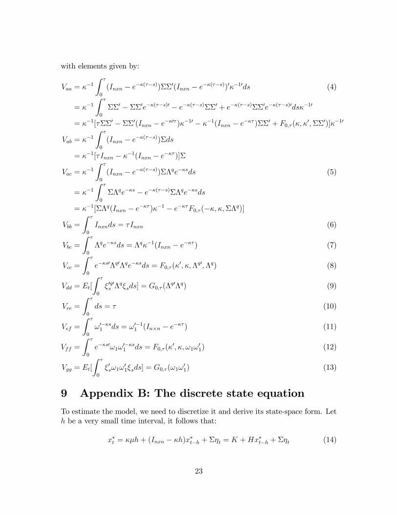
with elements given by:

Vaa = κ−1∫ τ

0

(Inxn − e−κ(τ−s))ΣΣ′(Inxn − e−κ(τ−s))′κ−1′ds (4)

= κ−1∫ τ

0

ΣΣ′ − ΣΣ′e−κ(τ−s)′ − e−κ(τ−s)ΣΣ′ + e−κ(τ−s)ΣΣ′e−κ(τ−s)′dsκ−1′

= κ−1[τΣΣ′ − ΣΣ′(Inxn − e−κ′τ )κ−1′ − κ−1(Inxn − e−κτ )ΣΣ′ + F0,τ (κ, κ′,ΣΣ′)]κ−1′

Vab = κ−1∫ τ

0

(Inxn − e−κ(τ−s))Σds

= κ−1[τInxn − κ−1(Inxn − e−κτ )]Σ

Vac = κ−1∫ τ

0

(Inxn − e−κ(τ−s))ΣΛqe−κsds (5)

= κ−1∫ τ

0

ΣΛqe−κs − e−κ(τ−s)ΣΛqe−κsds

= κ−1[ΣΛq(Inxn − e−κτ )κ−1 − e−κτF0,τ (−κ, κ,ΣΛq)]

Vbb =

∫ τ

0

Inxnds = τInxn (6)

Vbc =

∫ τ

0

Λqe−κsds = Λqκ−1(Inxn − e−κτ ) (7)

Vcc =

∫ τ

0

e−κs′Λq′Λqe−κsds = F0,τ (κ′, κ,Λq′,Λq) (8)

Vdd = Et[

∫ τ

0

ξ′q′s Λqξsds] = G0,τ (Λq′Λq) (9)

Vee =

∫ τ

0

ds = τ (10)

Vef =

∫ τ

0

ω′−κs1 ds = ω′−11 (In×n − e−κτ ) (11)

Vff =

∫ τ

0

e−κs′ω1ω′−κs1 ds = F0,τ (κ

′, κ, ω1ω′1) (12)

Vgg = Et[

∫ τ

0

ξ′sω1ω′1ξsds] = G0,τ (ω1ω

′1) (13)

9 Appendix B: The discrete state equation

To estimate the model, we need to discretize it and derive its state-space form. Leth be a very small time interval, it follows that:

x∗t = κµh+ (Inxn − κh)x∗t−h + Σηt = K +Hx∗t−h + Σηt (14)

23

where ηt ∼ N(0, hInxn). This means the discretized expression for the log price levelis:

qt = qt−h + ρπ0h+ ρπ′1 x∗t−hh+ λq(x∗t−h)

′ηt + ω(x∗t−h)η⊥t (15)

In order to capture the quadratic dynamics of real bond prices, we will have toaugment our state vector with the term vech(xtx

′t). We introduce the operator

Dn such that vec() = Dnvech(). We also introduce D+n = (D′nDn)−1D′n so that

D+n vec(x

∗tx∗′t ) = vech(x∗tx

∗′t ). Thus, applying properties of vec(),

vech(x∗tx∗′t ) = D+

n vec(KK′ + hΣΣ′) +D+

n (H ⊗K +K ⊗H)x∗t−h+D+

n (H ⊗H)vec(x∗t−hx∗′t−h) +D+

n vec(Σηtη′tΣ′

− hΣΣ′ + (K +Hx∗t−h)η′tΣ′ + Σηt(K

′ + x∗′t−hH′))

= vech(KK ′ + hΣΣ′) +D+n (H ⊗K +K ⊗H)x∗t−h

+D+n (H ⊗H)Dnvech(x∗t−hx

∗′t−h) + νt

where the errors terms are collected in

νt = D+n (Σ⊗ Σ)vec(ηtη

′t)− vech(hΣΣ′) +M(x∗t−h)Σηt (16)

andM(x∗t−h) = D+

n (Inxn ⊗ (K +Hx∗t−h) + (K +Hx∗t−h)⊗ Inxn) (17)

This permits us to define a linear state space equation:

st = Gh + Γhst−h + ηst (18)

in which:

st =

x∗tvech(x∗tx

∗′t )

qt

, Gh =

Kvech(KK ′ + hΣΣ′)

ρπ0h

, ηst =

Σηtνt

λq(x∗t−h)′ηt + ω(x∗t−h)η

⊥t

Γh =

H 0 0D+n (H ⊗K +K ⊗H) D+

n (H ⊗H)Dn 0ρπ′1 h 0 1

To perform Kalman filtering, we will need the conditional moments of the statevariables. We can easily see that

E[st|Ft−h] = Gh + Γhst−h (19)

The conditional variance Ωst−h = V ar(st|Ft−h) = V ar(ηst) = E[ηstη

s′t ].

24

10 Appendix C: Observation equations

Observed variables ot are linear in the underlying state vector:

ot = a+ Fst + εt (20)

Using the expression for the bond prices derived earlier (and solving the differentialequations), the continuously compounded yields can be expressed as:

Y Nt = aN + bN ′xt + εNt ,

where aN = [aN3m...aN10y]′ is the stacked vector of coeffi cients for each maturity, and

aNτ = − 1τANτ , where A

Nτ are the pricing parameters.

The short rate forecasts are f τt = Et[rt+τ ,3m] for τ = 6m, 12m. The 6-to-11years ahead forecast is f longt = 1

5

∫ 11y6y

Et[rt+τ ,3m]dτ . We can solve for these using ourexpressions for the yields to find:

f τt = an3m + bN ′3m(Inxn − e−κτ )µ+ bN ′3me−κτxt + εfτt (21)

f longt = aN3m + bN ′3m(Inxn −1

5κ−1(e−6κ − e−11κ))µ+ bN ′3m

1

5κ−1(e−6κ − e−11κ)xt + εflt

(22)

for τ = 6m, 12m.The inflation expectations can be expressed as:

EIτt = ρπ0 + ρπ′1 µ−1

τρπ′1 κ

−1(Inxn − e−κτ )µ+1

τρπ′1 κ

−1(Inxn − e−κτ )x∗t + εEIt (23)

for τ = 1, 11.Lastly, the one-year inflation uncertainty can be expressed:

IU1yt = C ′V C + (2C ′V D)x∗t + vec(D′V D)′Dnvech(x∗tx∗′t )) + εIUt

Thus, collecting all the coeffi cients of the constant terms in a and the coeffi cientsmultiplying the states in F , we have:

a =

0aN

af,6m

af,12m

af,l

ai,1yr

ai,10yr

au,1yr

F =

0 0 1bN ′ 0 0bf6m 0 0bf12m 0 0bfl 0 0bi,1yr 0 0bi,10yr 0 0bu,1yr vec(D′VτD)′Dn 0

(24)

The error vector εt will have a diagonal covariance matrix.

25

ReferencesAbrahams, M., T. Adrian, R. K. Crump, and E. Moench, 2013, “Decomposing realand nominal yield curves.”Federal Reserve Bank of New York Staff Reports No.570, October.

Ahn, D., Dittmar, R., and Gallant, A. (2002), "Quadratic term structure models:theory and evidence." Review of Financial Studies Vol. 15, No. 1, 243-288.

Ahn, D., Dittmar, R., Gallant, A., Gao, B. (2003), "Purebred or hybrid?: Repro-ducing the volatility in term structure dynamics." Journal of Econometrics 116,147—180

Ajello, Andrea, Luca Benzoni, and Olena Chyruk (2012), "Core and ’Crust’: Con-sumer Prices and the Term Structure of Interest Rates." Working Paper SeriesWP-2014-11. Federal Reserve Bank of Chicago.

Ang, A., G. Bekaert and M. Wei (2007), “Do macro variables, asset markets orsurveys forecast inflation better?”Journal of Monetary Economics, 54, 1163-212.

– – (2008), “The term structure of real rates and inflation expectations.”Journalof Finance, 63(2), 797—849.

Anh, Le and Kenneth J. Singleton (2013), “The Structure of Risks in EquilibriumAffi ne Models of Bond Yields.”Working paper, UNC.

Argov, Eyal, David Rose, Philippe Karam, Natan Epstein, and Douglas Laxton(2007). "Endogenous Monetary Policy Credibility in a Small Macro Model of Israel."IMF working paper 207.

Bansal, R. and Ivan Shaliastovich (2012), “A Long-Run Risks Explanation of Pre-dictability Puzzles in Bond and Currency Markets.”Review of Financial Studies.

Bekaert, Geert and Xiaozheng Wang (2010), “Inflation risk and the inflation riskpremium.”Economic Policy October 2010 pp. 755-806.

Buraschi, Andrea and Alexei Jiltsov (2005), “Inflation Risk Premia and the Expec-tations Hypothesis." Journal of Financial Economics 75, 429-490.

Campbell, J. Y. and R. Shiller (1996), “A scorecard for indexed government debt,”in B. S. Bernanke and J. Rotemberg (eds.), National Bureau of Economic ResearchMacroeconomics Annual 1996, MIT Press, Cambridge, MA, pp. 155—97.

Campbell J. Y., Sunderam A. and Viceira L., “Inflation bets or deflation hedges?The changing risks of nominal bonds.” Harvard Business School Working Paper,09-088, 2016.

Chernov, Mikhail, and Philippe Mueller (2012), "The term structure of inflationexpectations." Journal of Financial Economics vol. 106, 367-394.

26

Christensen, Jens H.E. , Jose A. Lopez, and Glenn D. Rudebusch (2012), “Extract-ing Deflation Probability Forecasts from Treasury Yields." International Journal ofCentral Banking, December, 21-60.

Cochrane, J. H. and Monika Piazzesi (2005), “Bond Risk Premia." American Eco-nomic Review, Vol. 94, No. 1, 138-160.

Collin-Dufresne, Pierre , Robert S. Goldstein, Christopher S. Jones, "Can inter-est rate volatility be extracted from the cross section of bond yields?" Journal ofFinancial Economics 94 (2009) 47-66.

Croushore, Dean (1993), “Introducing: The Survey of Professional Forecasters.”Federal Reserve Bank of Philadelphia Business Review, November/December, 3—13.

Dai, Q., Singleton, K. (2002), "Expectations puzzle, time-varying risk premia, andaffi ne models of the term structure." Journal of Financial Economics 63, 415—441

D’Amico, S., D. Kim and M. Wei (2016). "Tips from TIPS: the information contentof Treasury inflation-protected security prices", Journal of Financial and Quantita-tive Analysis, forthcoming.

D’Amico S., and Thomas King, (2015), "What does anticipated monetary policydo?" Federal Reserve Bank of Chicago Working Paper 2015-10.

D’Amico S., and Athanasios Orphanides (2008), “Uncertainty and Disagreement inEconomic Forecasting." Finance and Economics Discussion Series 2008-56. FederalReserve Board.

D’Amico S., and Athanasios Orphanides (2014), "Inflation Uncertainty and Dis-agreement in Bond Risk Premia." Federal Reserve Bank of Chicago Working PaperNo. 2014-24.

David, Alexander, and Pietro Veronesi (2013), “What Ties Return Volatilities toPrice Valuations and Fundamentals?" Journal of Political Economy, vol. 21, No. 4(August), 682-746.

Du, Wenxin, Carolin E. Pflueger, and Jesse Schreger (2016). "Sovereign Debt Port-folios, Bond Risks, and the Credibility of Monetary Policy." NBER Working PaperSeries, No. 22592, September.

Duffee, G. (2002), "Term premia and interest rate forecasts in affi ne models." Jour-nal of Finance 57, 405—443.

Duffee, G. (2011), “Information in (and not in) the term structure.” Review ofFinancial Studies 24, 2895-2934.

Evans, Charles, Jonas Fisher, Francois Gourio and Spencer Krane (2015), "Riskmanagement for monetary policy near the zero lower bound." Brookings Papers onEconomic Activity, March 19, 2015

27

Feldman, Ron, Kenneth Heinecke, Narayana Kocherlakota, Samuel Schulhofer-Wohl,and Thomas Tallarini (2016), "Market-Based Expectations as a Tool for Policymak-ers". Working Paper.

Goodfriend, Marvin (1993), "Interest Rate Policy and the Inflation Scare Problem:1979—1992." Reserve Bank of Richmond Economic Quarterly Volume 79/1 Winter1993.

Grishchenko, O. and J. Huang (2013), "The inflation risk premium: evidence fromthe TIPS market." The Journal of Fixed Income, Spring.

Gurkaynak, Refet S., Brian Sack, and Jonathan H. Wright (2006), “The U.S. Trea-sury Yield Curve: 1961 to the Present." Journal of Monetary Economics, vol. 54(8),2291-2304.

Gurkaynak, Refet S., and Jonathan H. Wright (2012), “Macroeconomics and theTerm Structure." Journal of Economic Literature, 50:2, 331-367.

Holston, Kathryn, Thomas Laubach and John C. Williams (2016), “Measuring theNatural Rate of Interest: International Trends and Determinants." Finance andEconomics Discussion Series, 2016-073. Washington: Board of Governors of theFederal Reserve System.

Haubrich Joseph, George Pennacchi, Peter Ritchken (2012). "Inflation Expecta-tions, Real Rates, and Risk Premia: Evidence from Inflation Swaps." Review ofFinacial Studies v.25, n 5, 1588-1629.

Joslin, Scott, Marcel Priebsch, and Kenneth J. Singleton (2014), "Risk Premiumsin Dynamic Term Structure Models with Unspanned Macro Risks." The Journal ofFinance, vol. LXIX(3), 1197-1233, June.

Kim, Don H. (2004), "Time-varying risk and return in the quadratic-gaussian modelof the term-structure." This paper is part of the author’s Stanford dissertation.

Kim, Don H. (2008), "Challenges in macro-finance modeling." Federal ReserveBoard Working Paper in the Finance and Economics Discussion Series 2008-06.

Kim, Don H. and Athanasios Orphanides (2012), “Term Structure Estimation withSurvey Data on Interest Rate Forecasts.” Journal of Financial and QuantitativeAnalysis, Volume 47, Issue 01, February 2012, 241-272.

Kim, Don H., and Kenneth J. Singleton (2012), "Term Structure Models and theZero Bound: An Empirical Investigation of Japanese Yields." Journal of Economet-rics, vol. 170, pp. 32-49.

Kim, H. D., Wright, J. H. (2005). “An Arbitrage-Free Three-Factor Term StructureModel and the Recent Behavior of Long-Term Yields and Distant-Horizon ForwardRates." Finance and Economics Discussion Series 2005-33. Federal Reserve Board.

28

Kitsul, Y. and Jonathan H. Wright, “The Economics of Options-Implied InfationProbability Density Functions." Journal of Financial Economics, forthcoming.

Longstaff, Francis A., Matthias Fleckenstein, and Hanno Lustig. (2014). "DeflationRisk". UCLA Working paper.

Palomino, Francisco (2012). "Bond Risk Premiums and Optimal Monetary Policy,"Review of Economic Dynamics, vol. 15, no. 1, pp. 19-40.

Piazzesi, Monika, and Martin Schneider (2006), “Equilibrium Yield Curves.”NBERWorking Paper 12609.

Piazzesi, Monika, Juliana Salomao, and Martin Schneider (2013), “Trend and Cyclein Bond Premia.”Working Paper, December.

Stark, Tom (2010), "Realistic Evaluation of Real-Time Forecasts in the Surveyof Professional Forecasters." Research Special Report, Federal Reserve Bank ofPhiladelphia, May.

Wachter, J. A. (2006), “A consumption-based model of the term structure of interestrates.”Journal of Financial Economics 79 (2), 365-399.

Wright, Jonathan H. (2011), “Term Premia and Inflation Uncertainty: EmpiricalEvidence from an International Panel Dataset." American Economic Review, 101(4),1514—34.

29

Table 1: R2 from regressions with nominal yield factors

Dependent Variable 1st factor 1st and 2nd factor 1st, 2nd, and 3rd factorπ .05 .06 .06E[π1y] .83 .84 .84E[π11y] .86 .86 .87V ar(π1y) .49 .49 .51

Note: Entries show the R2 of regressions of each of the inflation variables (in thefirst column) on the estimated factors from an affi ne term structure model.

Table 2: Summary of four alternative model specifications

Model Restrictions and IdentificationsModel Full ω1 unrestricted, Λq lower-triangular, ρN1 (3) = 0, ΛN

2×2Model No_TVV ω1 = 03×1, Λq = 03×3, ρ

N1 (3) = 0, ΛN

2×2Model No_IU δiu ≈ ∞, ω1 = 03×1, Λq lower-triangular, ρN1 (3) = 0, ΛN

2×2,Model No_Unsp ω1 unrestricted, Λq lower-triangular, ρN1 unrestricted, ΛN

3×3.

Table 3: R2 from regressing with full model’s factors

Dependent Variable 1st factor 1st and 2nd factor 1st, 2nd, and hidden factorπ .06 .06 .07E[π1y] .80 .83 .90E[π11y] .70 .84 .89V ar(π1y) .44 .47 .83

Note: Entries show the R2 of regressions of each of the inflation variables (in thefirst column) on the estimated factors x∗t from the full model.

30

1982 1984 1986 1988 1990 1992 1994 1996 1998 2000 2002 2004 2006 2008 2010 2012 2014

0

2

4

6

8

10

12

14

Nominal Yield Real Yield ExPi IRP

Figure 1: Decomposition of the 10-year zero-coupon nominal yield. Chart decom-poses the 10-year nominal yield into the 10-year real yield (including the RRP), theexpected inflation over the next 10 years (ExPi) and the corresponding IRP impliedby the full model.

31

1982 1984 1986 1988 1990 1992 1994 1996 1998 2000 2002 2004 2006 2008 2010 2012 2014-1

0

1

2

3

4

Expected Real Rate ExPi IRP RRP

Figure 2: Expectation components and risk premia in the 10-year zero-coupon nom-inal yield. Chart shows the expected average short-term real interest rate over thenext 10 years and the corresponding RRP together with the expected inflation overthe next 10 years (ExPi) and the corresponding IRP, implied by the full model.

32

1990 2000 2010

0.5

1

1.5

21 Yr Inflation Uncertainty

1990 2000 2010-2

0

2

4

6

85 Yr Real Yield

1990 2000 20100

2

4

6

1 Yr Expected Inflation

1990 2000 2010

0

5

10

1 Yr TBill Fcast

Figure 3: Overall Fit of the Full Model. Model estimates (in blue) compared withactual data and surveys (in orange). The top left panel plots the one-year survey-based inflation variance versus the model-implied inflation variance; the top rightpanel plots the 5-year actual TIPS yield versus the 5-year model-implied real yield;the bottom left panel plots the survey-based one-year expected inflation versus theone-year model-implied expected inflation; and the bottom right panel plots theone-year ahead survey forecast of the 3-month T-Bill rate versus the model-impliedone-year ahead expectation of the 3-month rate.

33

1990 2000 2010

Infl

Unc

er (

Pct

)

0.5

1

1.5

Homoskedastic Model

1990 2000 2010

0.51

1.5

Full Model

1990 2000 2010

2 Y

r IR

P (

Pct

)

-10

0

10

1990 2000 2010

-0.5

0

0.5

1990 2000 2010

5 Y

r R

Yld

(P

ct)

-100

10

1990 2000 2010

0246

1990 2000 2010

1 Y

r E

x In

f (P

ct)

2

4

1990 2000 2010

2

4

Figure 4: Comparison of homoskedastic and full models. The left panels show resultsfrom the model with homoskedastic inflation shocks and the right panels show thecorresponding results from the full model. The first row plots the estimated value ofthe one-year inflation variance and the one-year survey-based inflation uncertainty(orange). The second row plots the estimated two-year IRP. The third row plotsthe model-implied 5-year real yield and the actual 5-year TIPS yield (orange). Thelast row plots the estimated one-year expected inflation versus the one-year aheadsurvey forecast of inflation (orange).

34

1990 2000 2010

Ful

l Mod

el

-1

0

12 Yr IRP (Pct)

1990 2000 2010

0

1

210 Yr IRP (Pct)

1990 2000 2010

0.5

1

1.5

Infl Uncer (Pct)

1990 2000 2010

No

IU M

odel

-1

0

1

1990 2000 2010

0

1

2

1990 2000 2010

0.5

1

1.5

1990 2000 2010

No

UnS

p M

odel

0

2

4

1990 2000 2010

0

2

4

6

1990 2000 2010

0.5

1

1.5

Figure 5: Inflation Risk Premium Estimates and Model Fit of Inflation Uncertainty.Each row plot results from the Full Model, No IU Model, and No Unsp Model,respectively. The left and middle panels plot the estimated values of the 2-year and10-year IRP. The right panels plot the one-year model-implied inflation variancetogether its survey counterpart (orange).

35

1990 2000 2010

Ful

l Mod

el

0

4

810 Yr R Yield (Pct)

1990 2000 2010

0

2

410 Yr RRP (Pct)

1990 2000 2010

No

IU M

odel

0

4

8

1990 2000 2010

0

2

4

1990 2000 2010

No

UnS

p M

odel

0

4

8

1990 2000 2010-2

0

2

Figure 6: Model-Implied Real Yields versus TIPS yields and RRP Estimates. Eachrow plots results from the Full Model, No IU Model, and No Unsp Model, respec-tively. The left panels plot the model-implied 10-year real yield together with theactual 10-year TIPS yield (orange). The right panels plot the estimated values ofthe 10-year RRP.

36

1990 2000 2010

Ful

l Mod

el

2

4

6

Exp Inflation 1 Yr (Pct)

1990 2000 2010

2

4

6

Exp Inflation Over Next 11 Yr (Pct)

1990 2000 2010

No

IU M

odel

2

4

6

1990 2000 2010

2

4

6

1990 2000 2010

No

UnS

p M

odel

2

4

6

1990 2000 2010

2

4

6

Figure 7: Model Fit of Survey Inflation Expectations at one-year and 11-year hori-zons. Each row plots results from the Full Model, No IU Model, and No UnspModel, respectively. The left panels plot one-year model-implied inflation expecta-tion together with the corresponding survey forecast (orange). The right panels plotaverage model-implied inflation expectation over the next 11 years together with thecorresponding survey forecast (orange).

37

1990 2000 2010

Ful

l Mod

el

0

5

10

TBill Fcast 6 Mnth (Pct)

1990 2000 20102

4

6

8

Fwd Rate Fcast 6 to 11 Yr (Pct)

1990 2000 2010

No

IU M

odel

0

5

10

1990 2000 20102

4

6

8

1990 2000 2010

No

UnS

p M

odel

0

5

10

1990 2000 20102

4

6

8

Figure 8: Model Fit of Survey Forecasts of the Short Rate at short and long horizons.Each row plots results from the Full Model, No IU Model, and No Unsp Model,respectively. The left panels plot the 6-month-ahead model-implied expectation ofthe 3-month rate together with the 6-month-ahead survey forecast of the 3-monthT-Bill rate (orange). The right panels plot the 6-to-11 years ahead model-impliedexpectation of the 3-month rate together with the 6-to-11 years ahead survey forecastof the 3-month T-Bill rate (orange).

38

1

Working Paper Series

A series of research studies on regional economic issues relating to the Seventh Federal Reserve District, and on financial and economic topics.

The Urban Density Premium across Establishments WP-13-01 R. Jason Faberman and Matthew Freedman Why Do Borrowers Make Mortgage Refinancing Mistakes? WP-13-02 Sumit Agarwal, Richard J. Rosen, and Vincent Yao Bank Panics, Government Guarantees, and the Long-Run Size of the Financial Sector: Evidence from Free-Banking America WP-13-03 Benjamin Chabot and Charles C. Moul Fiscal Consequences of Paying Interest on Reserves WP-13-04 Marco Bassetto and Todd Messer Properties of the Vacancy Statistic in the Discrete Circle Covering Problem WP-13-05 Gadi Barlevy and H. N. Nagaraja Credit Crunches and Credit Allocation in a Model of Entrepreneurship WP-13-06 Marco Bassetto, Marco Cagetti, and Mariacristina De Nardi Financial Incentives and Educational Investment: The Impact of Performance-Based Scholarships on Student Time Use WP-13-07 Lisa Barrow and Cecilia Elena Rouse The Global Welfare Impact of China: Trade Integration and Technological Change WP-13-08 Julian di Giovanni, Andrei A. Levchenko, and Jing Zhang Structural Change in an Open Economy WP-13-09 Timothy Uy, Kei-Mu Yi, and Jing Zhang The Global Labor Market Impact of Emerging Giants: a Quantitative Assessment WP-13-10 Andrei A. Levchenko and Jing Zhang Size-Dependent Regulations, Firm Size Distribution, and Reallocation WP-13-11 François Gourio and Nicolas Roys Modeling the Evolution of Expectations and Uncertainty in General Equilibrium WP-13-12 Francesco Bianchi and Leonardo Melosi Rushing into the American Dream? House Prices, the Timing of Homeownership, and the Adjustment of Consumer Credit WP-13-13 Sumit Agarwal, Luojia Hu, and Xing Huang

2

Working Paper Series (continued) The Earned Income Tax Credit and Food Consumption Patterns WP-13-14 Leslie McGranahan and Diane W. Schanzenbach Agglomeration in the European automobile supplier industry WP-13-15 Thomas Klier and Dan McMillen Human Capital and Long-Run Labor Income Risk WP-13-16 Luca Benzoni and Olena Chyruk The Effects of the Saving and Banking Glut on the U.S. Economy WP-13-17 Alejandro Justiniano, Giorgio E. Primiceri, and Andrea Tambalotti A Portfolio-Balance Approach to the Nominal Term Structure WP-13-18 Thomas B. King Gross Migration, Housing and Urban Population Dynamics WP-13-19 Morris A. Davis, Jonas D.M. Fisher, and Marcelo Veracierto Very Simple Markov-Perfect Industry Dynamics WP-13-20 Jaap H. Abbring, Jeffrey R. Campbell, Jan Tilly, and Nan Yang Bubbles and Leverage: A Simple and Unified Approach WP-13-21 Robert Barsky and Theodore Bogusz The scarcity value of Treasury collateral: Repo market effects of security-specific supply and demand factors WP-13-22 Stefania D'Amico, Roger Fan, and Yuriy Kitsul Gambling for Dollars: Strategic Hedge Fund Manager Investment WP-13-23 Dan Bernhardt and Ed Nosal Cash-in-the-Market Pricing in a Model with Money and Over-the-Counter Financial Markets WP-13-24 Fabrizio Mattesini and Ed Nosal An Interview with Neil Wallace WP-13-25 David Altig and Ed Nosal Firm Dynamics and the Minimum Wage: A Putty-Clay Approach WP-13-26 Daniel Aaronson, Eric French, and Isaac Sorkin Policy Intervention in Debt Renegotiation: Evidence from the Home Affordable Modification Program WP-13-27 Sumit Agarwal, Gene Amromin, Itzhak Ben-David, Souphala Chomsisengphet, Tomasz Piskorski, and Amit Seru

3

Working Paper Series (continued) The Effects of the Massachusetts Health Reform on Financial Distress WP-14-01 Bhashkar Mazumder and Sarah Miller Can Intangible Capital Explain Cyclical Movements in the Labor Wedge? WP-14-02 François Gourio and Leena Rudanko Early Public Banks WP-14-03 William Roberds and François R. Velde Mandatory Disclosure and Financial Contagion WP-14-04 Fernando Alvarez and Gadi Barlevy The Stock of External Sovereign Debt: Can We Take the Data at ‘Face Value’? WP-14-05 Daniel A. Dias, Christine Richmond, and Mark L. J. Wright Interpreting the Pari Passu Clause in Sovereign Bond Contracts: It’s All Hebrew (and Aramaic) to Me WP-14-06 Mark L. J. Wright AIG in Hindsight WP-14-07 Robert McDonald and Anna Paulson On the Structural Interpretation of the Smets-Wouters “Risk Premium” Shock WP-14-08 Jonas D.M. Fisher Human Capital Risk, Contract Enforcement, and the Macroeconomy WP-14-09 Tom Krebs, Moritz Kuhn, and Mark L. J. Wright Adverse Selection, Risk Sharing and Business Cycles WP-14-10 Marcelo Veracierto Core and ‘Crust’: Consumer Prices and the Term Structure of Interest Rates WP-14-11 Andrea Ajello, Luca Benzoni, and Olena Chyruk

The Evolution of Comparative Advantage: Measurement and Implications WP-14-12 Andrei A. Levchenko and Jing Zhang Saving Europe?: The Unpleasant Arithmetic of Fiscal Austerity in Integrated Economies WP-14-13 Enrique G. Mendoza, Linda L. Tesar, and Jing Zhang Liquidity Traps and Monetary Policy: Managing a Credit Crunch WP-14-14 Francisco Buera and Juan Pablo Nicolini Quantitative Easing in Joseph’s Egypt with Keynesian Producers WP-14-15 Jeffrey R. Campbell

4

Working Paper Series (continued) Constrained Discretion and Central Bank Transparency WP-14-16 Francesco Bianchi and Leonardo Melosi Escaping the Great Recession WP-14-17 Francesco Bianchi and Leonardo Melosi More on Middlemen: Equilibrium Entry and Efficiency in Intermediated Markets WP-14-18 Ed Nosal, Yuet-Yee Wong, and Randall Wright Preventing Bank Runs WP-14-19 David Andolfatto, Ed Nosal, and Bruno Sultanum The Impact of Chicago’s Small High School Initiative WP-14-20 Lisa Barrow, Diane Whitmore Schanzenbach, and Amy Claessens Credit Supply and the Housing Boom WP-14-21 Alejandro Justiniano, Giorgio E. Primiceri, and Andrea Tambalotti The Effect of Vehicle Fuel Economy Standards on Technology Adoption WP-14-22 Thomas Klier and Joshua Linn What Drives Bank Funding Spreads? WP-14-23 Thomas B. King and Kurt F. Lewis Inflation Uncertainty and Disagreement in Bond Risk Premia WP-14-24 Stefania D’Amico and Athanasios Orphanides Access to Refinancing and Mortgage Interest Rates: WP-14-25 HARPing on the Importance of Competition Gene Amromin and Caitlin Kearns Private Takings WP-14-26 Alessandro Marchesiani and Ed Nosal Momentum Trading, Return Chasing, and Predictable Crashes WP-14-27 Benjamin Chabot, Eric Ghysels, and Ravi Jagannathan Early Life Environment and Racial Inequality in Education and Earnings in the United States WP-14-28 Kenneth Y. Chay, Jonathan Guryan, and Bhashkar Mazumder Poor (Wo)man’s Bootstrap WP-15-01 Bo E. Honoré and Luojia Hu

Revisiting the Role of Home Production in Life-Cycle Labor Supply WP-15-02 R. Jason Faberman

5

Working Paper Series (continued) Risk Management for Monetary Policy Near the Zero Lower Bound WP-15-03 Charles Evans, Jonas Fisher, François Gourio, and Spencer Krane Estimating the Intergenerational Elasticity and Rank Association in the US: Overcoming the Current Limitations of Tax Data WP-15-04 Bhashkar Mazumder External and Public Debt Crises WP-15-05 Cristina Arellano, Andrew Atkeson, and Mark Wright The Value and Risk of Human Capital WP-15-06 Luca Benzoni and Olena Chyruk Simpler Bootstrap Estimation of the Asymptotic Variance of U-statistic Based Estimators WP-15-07 Bo E. Honoré and Luojia Hu Bad Investments and Missed Opportunities? Postwar Capital Flows to Asia and Latin America WP-15-08 Lee E. Ohanian, Paulina Restrepo-Echavarria, and Mark L. J. Wright Backtesting Systemic Risk Measures During Historical Bank Runs WP-15-09 Christian Brownlees, Ben Chabot, Eric Ghysels, and Christopher Kurz What Does Anticipated Monetary Policy Do? WP-15-10 Stefania D’Amico and Thomas B. King Firm Entry and Macroeconomic Dynamics: A State-level Analysis WP-16-01 François Gourio, Todd Messer, and Michael Siemer Measuring Interest Rate Risk in the Life Insurance Sector: the U.S. and the U.K. WP-16-02 Daniel Hartley, Anna Paulson, and Richard J. Rosen Allocating Effort and Talent in Professional Labor Markets WP-16-03 Gadi Barlevy and Derek Neal The Life Insurance Industry and Systemic Risk: A Bond Market Perspective WP-16-04 Anna Paulson and Richard Rosen Forecasting Economic Activity with Mixed Frequency Bayesian VARs WP-16-05 Scott A. Brave, R. Andrew Butters, and Alejandro Justiniano Optimal Monetary Policy in an Open Emerging Market Economy WP-16-06 Tara Iyer Forward Guidance and Macroeconomic Outcomes Since the Financial Crisis WP-16-07 Jeffrey R. Campbell, Jonas D. M. Fisher, Alejandro Justiniano, and Leonardo Melosi

6

Working Paper Series (continued) Insurance in Human Capital Models with Limited Enforcement WP-16-08 Tom Krebs, Moritz Kuhn, and Mark Wright Accounting for Central Neighborhood Change, 1980-2010 WP-16-09 Nathaniel Baum-Snow and Daniel Hartley The Effect of the Patient Protection and Affordable Care Act Medicaid Expansions on Financial Wellbeing WP-16-10 Luojia Hu, Robert Kaestner, Bhashkar Mazumder, Sarah Miller, and Ashley Wong The Interplay Between Financial Conditions and Monetary Policy Shock WP-16-11 Marco Bassetto, Luca Benzoni, and Trevor Serrao Tax Credits and the Debt Position of US Households WP-16-12 Leslie McGranahan The Global Diffusion of Ideas WP-16-13 Francisco J. Buera and Ezra Oberfield Signaling Effects of Monetary Policy WP-16-14 Leonardo Melosi Constrained Discretion and Central Bank Transparency WP-16-15 Francesco Bianchi and Leonardo Melosi Escaping the Great Recession WP-16-16 Francesco Bianchi and Leonardo Melosi The Role of Selective High Schools in Equalizing Educational Outcomes: Heterogeneous Effects by Neighborhood Socioeconomic Status WP-16-17 Lisa Barrow, Lauren Sartain, and Marisa de la Torre Monetary Policy and Durable Goods WP-16-18 Robert B. Barsky, Christoph E. Boehm, Christopher L. House, and Miles S. Kimball Interest Rates or Haircuts? Prices Versus Quantities in the Market for Collateralized Risky Loans WP-16-19 Robert Barsky, Theodore Bogusz, and Matthew Easton Evidence on the within-industry agglomeration of R&D, production, and administrative occupations WP-16-20 Benjamin Goldman, Thomas Klier, and Thomas Walstrum Expectation and Duration at the Effective Lower Bound WP-16-21 Thomas B. King

7

Working Paper Series (continued) The Term Structure and Inflation Uncertainty WP-16-22 Tomas Breach, Stefania D’Amico, and Athanasios Orphanides