This paper presents preliminary findings and is being distributed to economists

and other interested readers solely to stimulate discussion and elicit comments.

The views expressed in this paper are those of the author and are not necessarily

reflective of views at the Federal Reserve Bank of New York or the Federal

Reserve System. Any errors or omissions are the responsibility of the author.

Federal Reserve Bank of New York

Staff Reports

Option-Implied Term Structures

Erik Vogt

Staff Report No. 706

December 2014

Revised January 2016

Option-Implied Term Structures

Erik Vogt

Federal Reserve Bank of New York Staff Reports, no. 706

December 2014; revised January 2016

JEL classification: G12, G17, C58

Abstract

This paper proposes a nonparametric sieve regression framework for pricing the term structure of

option spanning portfolios. The framework delivers closed-form, nonparametric option pricing

and hedging formulas through basis function expansions that grow with the sample size. Novel

confidence intervals quantify term structure estimation uncertainty. The framework is applied to

estimating the term structure of variance risk premia and finds that a short-run component

dominates market excess return predictability. This finding is inconsistent with existing asset

pricing models that seek to explain the variance risk premium’s predictive content.

Key words: variance risk premium, term structures, options, return predictability, nonparametric

regression.

_________________

Vogt: Federal Reserve Bank of New York (e-mail: erik.vogt@ny.frb.org). The author is

especially thankful to his dissertation chair, George Tauchen, and his dissertation committee

members, Tim Bollerslev, Federico Bugni, Jia Li, and Andrew Patton, for their guidance and

encouragement. He is also grateful to Tobias Adrian, Torben Andersen, Gurdip Bakshi, Nina

Boyarchenko, Michael Brandt, Peter Christoffersen, Richard Crump, Ron Gallant, Steve Heston,

Roger Koenker, Ralph Koijen, Pete Kyle, Simon (Sokbae) Lee, Adam McCloskey, Eric Renault,

Matthew Richardson, Alberto Rossi, Enrique Sentana, Peter Van Tassel, and Dacheng Xiu, as

well as seminar participants at Duke, the Federal Reserve Bank of New York, the Federal

Reserve Board, Brown University, London Business School, the University of Illinois at Urbana-

Champaign, the University of Maryland, the 2013 Triangle Econometrics Conference, AQR,

Citadel, PDT Partners, QMS Capital Management, and the 2015 Econometric Society World

Congress, for valuable comments and suggestions. All errors are those of the author. The views

expressed in this paper are those of the author and are not necessarily reflective of views at the

Federal Reserve Bank of New York or the Federal Reserve System.

1 Introduction

When an asset’s cash flows are expected to occur at multiple future dates, the prices of each

individual cash flow form a term structure. While term structures are traditionally studied for

assets with a predetermined sequence of cash flows (as with risk-free bonds), a flurry of recent

research has expanded into studying the term structures of a wider array of risky assets.1 This

paper studies term structures of risky assets whose cash flows depend on future realized moments

of another reference security, with a particular focus on realized variances, their prices, and risk

premia.

Measuring the prices of long-run variance and other realized moments is challenging. While the-

oretical hedging arguments show that integrated portfolios of call and put options price (or “span”)

these moments, long-dated options are generally illiquid, meaning that the valuations obtained from

integrated hedging portfolios must be inferred from a handful of noisy options. How well do illiquid,

long-dated option-spanning portfolios approximate risk-neutral expectations of long-run realized

moments? Understanding the answer to this question is of first-order importance for interpreting

risk premia in the term structures of realized moments.

This paper makes a methodological contribution toward measuring long-run risk-neutral ex-

pectations of variance and other moments from options. By forming basis function expansions of

the state-price density, the paper derives new closed-form option prices that can be interpreted as

nonparametric extensions of the Black and Scholes (1973) formula. While these option prices are po-

tentially of independent interest (for example for hedging purposes), they are particularly suited to

the problem of estimating the term structures of risk-neutral moments: First, they inject theoretical

structure into estimated option prices while remaining nonparametric. This theoretical structure

helps connect estimates of long-run option spanning portfolios to the information contained in liquid

short-maturity options. Second, they allow for a novel theory of inference that allows one to obtain

confidence intervals for the term structures of realized moments, thereby quantifying the precision

with which long-run risk-neutral moments can be priced with illiquid options. In a first application

of the inference result, we find that there is substantially higher estimation uncertainty around

long-run risk-neutral skewness and kurtosis than for long-run risk-neutral variance.2 Moreover, we1See Van Binsbergen and Koijen (2015) for a survey.2See Conrad, Dittmar, and Ghysels (2013) and Bakshi, Kapadia, and Madan (2003) for studies of skewness and

1

find that the term structures of second, third, and fourth risk-neutral moments have a strong factor

structure that loads heavily on variance factors (i.e. the VIX term structure).

The paper’s empirical focus on variance is therefore motivated by the factor structure result on

higher order moments, as well as recent research on the term structure of variance risk premia: by

examining Sharpe ratios of trading strategies that effectively sell variance along its term structure,

Dew-Becker, Giglio, Le, and Rodriguez (2015) have found that only news about short-run realized

variance is priced. In related work, Andries, Eisenbach, Schmalz, and Wang (2015) use the Heston

(1993) model and a short option straddle to estimate the term structure of variance risk premia,

an object also studied in Aït-Sahalia, Karaman, and Mancini (2015), who find a significant price-

jump component in their own estimated term structure of variance risk premia. These papers join

a growing literature on understanding risk premia in the term structures of assets beyond fixed

income which includes van Binsbergen, Brandt, and Koijen (2012) and van Binsbergen, Hueskes,

Koijen, and Vrugt (2013), who decompose the equity premium into its term structure components.

All of these papers find that risk premia are downward sloping in absolute value, that is, that a

short-run component dominates equity and variance risk premia. Since several leading asset pricing

benchmarks have counterfactual implications for the term structure of risk premia, these findings

present something of a puzzle to current models in finance.3

This paper presents new findings on the relationship between variance risk premia and equity

market return predictability. Motivated by Bollerslev, Tauchen, and Zhou (2009)’s and Drechsler

and Yaron (2011)’s findings that the one-month variance risk premium (VRP) predicts equity market

excess returns, we examine the predictive ability of long-run variance risk premia. We find that while

long-run variance risk premia strongly predict returns, the predictability is largely generated by a

short-run component. This is the result of predictive regressions that additively decompose long-

run VRP into the sum of one-month VRP and a forward VRP that represents compensation that

investors earn for exposure to variance risk beyond the first month. The predictive results connect

the findings of Dew-Becker, Giglio, Le, and Rodriguez (2015) and Andries, Eisenbach, Schmalz,

and Wang (2015) to the findings of van Binsbergen, Brandt, and Koijen (2012) by showing that

kurtosis option-spanning portfolios that are based on the spanning theorems of Bakshi and Madan (2000).3For instance, the long-run risk model of Bansal and Yaron (2004) and the habit formation model of Campbell

and Cochrane (1999) have equity risk premia that are counterfactually upward sloping in the term structure, and thelong-run risk model of Drechsler and Yaron (2011) has a variance risk premium term structure that does not accountfor the steep risk premium at the one month horizon and subsequent flatness for remaining horizons.

2

discount rates for short-term variance cash flows are tightly linked to those of the equity term

structure, which in turn are tied to discount rates of short-term dividend cash flows.

The predictive results present a challenge to the return predictability theories of Bollerslev,

Tauchen, and Zhou (2009) and Drechsler and Yaron (2011). In the Bollerslev, Tauchen, and

Zhou (2009) equilibrium framework, for example, recursive preferences combined with time-varying

volatility of consumption volatility (consumption vol-of-vol) imply that the equity premium and the

variance risk premium are linked by the same consumption vol-of-vol process qt. Similarly, in the ex-

tended long-run risk model of Drechsler and Yaron (2011), this link is established by a time-varying

aggregate stochastic volatility process σ2t that is common to all state variables in their economy.

Because it can be shown that the same process (qt for Bollerslev, Tauchen, and Zhou (2009) and

σ2t for Drechsler and Yaron (2011)) also governs variation in forward VRP, both models suggest

that forward VRP should also predict equity market excess returns. However, the predictive results

presented in Section 4 below show that this is not the case, since the forward VRP by itself does

not predict returns. The predictive results suggest that the factors driving time variation in the

one-month VRP must be distinct from those that drive forward VRP and, furthermore, that only

the one-month VRP factors are priced in equity returns. Therefore, the empirical results presented

in this paper provide guidance for equilibrium asset pricing models that seek to explain the link

between discount rates for variance-linked cash flows and discount rates for equity cash flows.

To study the long-run properties of risk-neutral realized moments, this paper presents the first

sieve application to option pricing. The method of sieves is a nonparametric alternative to kernel

methods that have been used in option pricing (e.g. Aït-Sahalia and Lo (1998)) and can therefore

be viewed as complementary. One advantage of sieve-based methods is that many quantities in

finance are concerned with computing expectations where the only object missing is the density

over possible future states, but the remaining objects involved in the expectation are known. Sieve-

based methods allow the direct expansion of the unknown density, and hence should present a useful

alternative tool to computing the many expectations that are prevalent in finance. Moreover, since

the method of sieve allows some discretion in the choice of basis function expansion, the results are

often closed-form expressions. One such expression is presented in this paper, in which option prices

appear as Black-Scholes prices plus higher order expansion terms that account for non-lognormality

of the underlying asset. Formulas of this type additionally have implications for hedging, since the

3

expansion terms correct local misspecification of Black-Scholes option prices, to the extent that

non-lognormalities are present.

The outline of the paper is as follows. Section 2 presents the methodological contribution for

measuring option-implied term structures. Section 3 shows its validity in a brief simulation exercise,

and Section 4 presents the main empirical findings.

2 Measuring Long-Run Risk-Neutral Expectations

This section develops a framework for estimating long-run risk-neutral expectations of realized

moments that explicitly recognizes illiquidity issues in long-maturity options. For exposition, the

focus is on risk-neutral variance; higher order moments are presented at the end of this section.

The general idea in what follows is to exploit existing option-spanning relationships together with

shape information in options.

Standing at time 0, consider the problem of measuring the risk-neutral expectation of realized

variance EQ0 [RV0,τ ], where RV0,τ measures the sum of squared returns of a reference asset from now

until time τ . Well-known spanning results imply that the synthetic variance swap (SVS) provides

a good hedge, i.e. SV S0(τ) = EQ0 [RV0,τ ] up to a third-order approximation error (Carr and Wu

(2009)). For a given time horizon τ , the SVS is obtained by combining European put and call options

with different strikes κ and common maturity τ into a single portfolio. Letting Z = (κ, τ, r, q), where

r ≡ r(τ) and q ≡ q(τ) correspond to the risk-free rate and underlying dividend yield at the maturity

τ of interest, the SVS term structure is the function

SV S0(τ) =2

τerτ∫ F (Z)

0

1

κ2P0(Z)dκ+

2

τerτ∫ ∞F (Z)

1

κ2C0(Z)dκ, (1)

where F (Z) = S0e(r−q)τ is the forward price, S0 is the current (fixed) stock price, P0(Z) is the put

option price with characteristics Z, and C0(Z) = P0(Z) +S0e−qτ −κe−rτ is the call option price by

put-call parity. We therefore need to evaluate P0(Z) at arbitrary τ across an infinite continuum of

κ in order to get at the portfolio term structure SV S0(τ) and thereby measure EQ0 [RV0,τ ].

Because P0(Z) (and therefore C0(Z) by put-call parity) is unobserved, it must be estimated

from a sample of put option prices and characteristics Pi,Zini=1. Table 1 shows that a typical

4

Table 1: Sample Averages for Monthly S&P 500 Index Options, 1996-2013.

Maturity Range Number of Option Open Bid-Ask(Days) Options Volume Interest Spread ($)

0 - 90 196.2 188 952.6 2 403 231.7 0.9690 - 180 59.6 20 325.3 702 530.5 1.19180 - 270 45.4 8626.8 434 287.5 1.38270 - 360 42.4 4770.0 260 077.3 1.61360 - 450 16.8 2180.6 161 567.9 1.97450 - 540 16.5 1131.8 122 241.0 2.13540 - 630 12.6 751.0 83 417.1 2.35630 - 720 12.3 810.5 63 685.1 2.42720 - ∞ 18.7 1521.4 90 235.1 4.46

0 - ∞ 420.9 229 072.0 4 321 320.0 1.35

cross-section of S&P 500 index options, some of the most liquid option contracts available, contains

about n = 420 prices, with most of the observations concentrated at short maturities. The thinning

of available option quotes for increasing τ is also associated with smaller trading volumes, less

open interest, and widening bid-ask spreads.4 The widening spreads introduce varying levels of

uncertainty about P0(Z) for different τ , which we allow for by letting Pi = P0(Zi) + εi for εi a

conditionally mean-zero, heteroskedastic measurement error. In this context, we refer to P0(Zi) as

representing the true option price for an option with characteristics Zi. Collectively, we follow the

literature and refer to the thinning of prices and increased noise as manifestations of illiquidity at

longer maturities.5

2.1 Theoretical Structure to Inform Long-Run Expectations

To preserve the SVS’s interpretation as a model-free spanning portfolio, P0(Z) is estimated nonpara-

metrically. However, the illiquidity of long-maturity options suggests that they are less informative

about long-run SVS, requiring the need for additional information. For added structure, the pro-

posed framework therefore relies on the risk-neutral valuation equation, which states that there

exists a conditional density f0 such that P0(Z) = P (f0,Z) for known P (·,Z).4Note that Table 1 reports dollar bid-ask spreads because dollar values enter the integral in (1). The data set

follows the CBOE data filters and is discussed further in Section 4.5See, e.g. Aït-Sahalia, Karaman, and Mancini (2015) and Driessen, Maenhout, and Vilkov (2009) for papers that

express concerns about this illiquidity when studying long-run risk-neutral moments.

5

Formally, for a vector of characteristics Z = (κ, τ, r, q), the true option price is modeled as

P0(Z) ≡ e−rτEQ0

[[κ− S

]+

∣∣∣τ,V = v0

]= e−rτ

∫ κ

0[κ− S]fQ0 (S|τ,V = v0)dS, (2)

where V is a vector of state variables that generate the current information set, fQ0 ( · |τ,V = v0)

is the unobserved state-price density (SPD), r is the risk-free rate, and S is the random (future)

value of the underlying. The components of V are left unspecified and can contain any number of

variables relevant to pricing options. The Heston model, for example, specifies V = (S0, V0), where

S0 is the current underlying price and V0 represents spot volatility (see Heston (1993), Duffie, Pan,

and Singleton (2000)).

Since the data represent an option cross-section at a single point in time, V realizes to some

fixed value V = v0. To simplify notation, we therefore define fQ0 (S|τ) ≡ fQ0 (S|τ,V = v0), since v0

is static across the option surface. On the other hand, τ is not static on the option surface because

it indexes maturity. In this form, the risk-neutral valuation formula on a single option cross-section

becomes

P0(Z) ≡ e−rτ∫ κ

0[κ− S]fQ0 (S|τ) dS. (3)

The dependence of the option price on the SPD fQ0 and the characteristics Z can be expressed as

PS(fQ0 ,Z) ≡ P0(Z).

The no-arbitrage pricing equation (3) implies shape restrictions on the option prices. Dif-

ferentiating PS(fQ0 ,Z) repeatedly with respect to the strike price κ yields the conditions ∂PS∂κ =

e−rτFQ0 (κ|τ) and ∂2PS

∂κ2= e−rτfQ0 (κ|τ), where FQ

0 is the CDF of fQ0 . These conditions immedi-

ately imply that PS(fQ0 ,Z) is monotone and convex in κ for any τ , and additionally has slope e−rτ

as κ → ∞ and slope 0 as κ → 0. Notice that these shape constraints follow directly from the

nonnegativity of fQ0 and the property that fQ0 integrates to one with respect to S for all τ .6

Since the option price’s shape constraints are implied by the fact that fQ0 is a PDF, the strat-

egy employed for obtaining shape-conforming option price estimates is the use of basis function6These shape constraints have been exploited elsewhere in the nonparametric option pricing literature for a single

τ . See, for example, Aït-Sahalia and Duarte (2003), Bondarenko (2003), Yatchew and Härdle (2006), and Figlewski(2008).

6

expansions that are valid PDFs. However, instead of approximating fQ0 directly, it turns out that

a convenient change of variables will lead to theoretically appealing closed-form option prices. To

this end, let Y be the random variable that satisfies

log

(S

S0

)= µ(Z) + σ(Z)Y, (4)

where Y |τ has density f0(y|τ), and µ(·) and σ(·) > 0 are known functions of the characteristics Z,

and where f0(·|τ) is the unknown density to be nonparametrically estimated from the data. This

change of variables is always possible for S > 0 because for any µ(·) and σ(·), Y simply is the

variable that makes (4) hold.

Under this change of variables, the valuation equation (3) becomes

PS(fQ0 ,Z) = e−rτ∫ κ

0

(κ− S

)fQ0 (S|τ) dS = e−rτ

∫ d(Z)

0

(κ− S0eµ(Z)+σ(Z)Y

)f0(Y |τ) dY ≡ P (f0,Z),

(5)

where

d(Z) =log(κ/S0)− µ(Z)

σ(Z)(6)

and

fQ0 (κ|τ) = (κσ(Z))−1f0(d(Z)|τ) (7)

follow from a Jacobian transformation.

Since (5) says PS(fQ0 ,Z) = P (f0,Z), one can focus on option pricing equations of the form

P (f,Z) = e−rτ∫ d(Z)

0

(κ− S0eµ(Z)+σ(Z)Y

)f(Y |τ) dY. (8)

It is easy to verify that (8) satisfies the same shape restrictions as (3) for any f with f(y|τ) ≥ 0

and∫f(y|τ)dy = 1.

2.2 Estimation and Option Pricing

Because the shape information comes from the fact that f0 is a density for any τ , we only need to

consider P (f,Z) for candidates f that are valid densities. Denote the collection of these candidate

7

densities by F . The method of sieves then implies that option prices can be estimated by solving

fKn = arg minf∈FKn

1

n

n∑i=1

[Pi − P (f,Zi)

]2W (Zi)

, (9)

where FKn ⊂ F is a member of a sequence of compact approximating spaces FK∞K=1 that grow

slowly in dimension (Kn → ∞) as the sample size n → ∞, eventually becoming dense in F .

Informally, as the sample size grows, the approximating spaces FKn increasingly resemble the parent

space F , so that the solution on FKn should converge to f0. Proposition 3 in the Appendix makes

this notion precise and further shows that the option price estimates P (Z) ≡ P (fKn ,Z) also converge

to the true option price P (f0,Z).7

The elements of FKn are obtained as follows. Since Gallant and Nychka (1987) have shown that

squared Hermite polynomials are suitable approximations for smooth joint densities, we can use

their densities,

fY,τK (y, τ) =

Ky∑k=0

Kτ∑j=0

βkjHj(τ)

Hk(y)

2

e−τ2/2e−y

2/2 =

Ky∑k=0

αk(B, τ)Hk(y)

2

e−τ2/2e−y

2/2,

(10)

where B is a matrix of coefficients with kj-entry βkj and K = (Ky + 1)(Kτ + 1).8 Thus, we can

form ratios to obtain closed-form conditional densities

fK(y|τ) = fY,τK (y, τ)

/∫fY,τK (y, τ)dy =

2Ky∑k=0

γk(B, τ)Hk(y)φ(y), (11)

7As written, the objective function in (9) is in dollar levels, which weights at-the-money options highest. Tosee this, let I(Zi) = erτ max[κi − S0, 0] denote the intrinsic value of option i. Then [Pi − P (f,Zi)]

2 = [Pi −I(Zi)−P (f,Zi)− I(Zi)]2. Because Pi− I(Zi) and P (f,Zi)− I(Zi) assume their largest values at-the-money,the objective function in (14) is most sensitive to deviations at-the-money. If a different weighting is desired, thefunction W (Zi) can be used instead. For example, by setting W (Zi) to the inverse of option i’s squared vega, onecan approximate implied volatility errors (e.g., Christoffersen, Fournier, and Jacobs (2013)). However, for inferenceproblems related to option-implied term structures, the Monte Carlo simulations provided in the Online Appendixsuggest that simply setting W (Zi) = 1 yields superior coverage properties.

8The Hermite polynomials are orthogonalized polynomials. They are defined, for scalars x, by

HK(x) =xHK−1(x)−

√K − 1HK−2(x)√K

, K ≥ 2

where H0(x) = 1, and H1(x) = x [see, for example, León, Mencía, and Sentana (2009)]. Note that HK(x) is apolynomial in x of degree K.

8

where the second equality is derived in Lemma B.1 and γk(B, τ) is a known function. Consequences

of this choice of basis functions are closed-form option prices.

Proposition 1. For a candidate SPD fK(y|τ) ∈ FK of the form given in equation (40), the put

option price P (fK ,Z) from equation (8) is given by

P (fK ,Z) = κe−rτ

Φ(d(Z))−2Ky∑k=1

γk(B, τ)√k

Hk−1(d(Z))φ(d(Z))

− S0e−rτ+µ(Z)

eσ(Z)2/2Φ(d(Z)− σ(Z)) +

2Ky∑k=1

γk(B, τ)I∗k(d(Z))

(12)

where Φ(·) is the standard normal CDF, K = (Ky + 1)(Kτ + 1), and where

I∗k(d(Z)) =σ(Z)√kI∗k−1(d(Z))− 1√

keσ(Z)d(Z)Hk−1(d(Z))φ(d(Z)), for k ≥ 1,

I∗0 (d(Z)) = eσ(Z)2/2Φ(d(Z)− σ(Z)),

and γk(B, τ) is the coefficient function given in equation (40).

The price of a call option is given by

C(fK ,Z) = S0e−rτ+µ(Z)

eσ(Z)2/2[1− Φ(d(Z)− σ(Z))]−2Ky∑k=1

γk(B, τ)I∗k(d(Z))

− κe−rτ

[1− Φ(d(Z))]−2Ky∑k=1

γk(B, τ)√k

Hk−1(d(Z))φ(d(Z))

. (13)

Proof. Appendix B.

With this result in hand, (9) becomes computationally equivalent to nonlinear least squares with

known regressors,

βn = arg minβ∈RKn

1

n

n∑i=1

[Pi − P (β,Zi)

]2W (Zi)

, (14)

where β ≡ vec(B) and where P (β,Z) ≡ P (fK ,Z) is the option pricer in (12) as a function of

9

the basis function coefficients. Finally, it can be shown that by imposing∑Ky(n)

k=0

∑Kτ (n)j=0 β2kj = 1

during estimation, the fK(y|τ) will integrate to one for all τ , resulting in option prices P (Z) that

incorporate shape information (as required for long maturities).

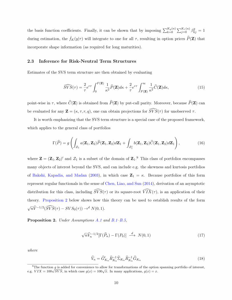
2.3 Inference for Risk-Neutral Term Structures

Estimates of the SVS term structure are then obtained by evaluating

SV S(τ) =2

τerτ∫ F (Z)

0

1

κ2P (Z)dκ+

2

τerτ∫ ∞F (Z)

1

κ2C(Z)dκ, (15)

point-wise in τ , where C(Z) is obtained from P (Z) by put-call parity. Moreover, because P (Z) can

be evaluated for any Z = (κ, τ, r, q), one can obtain projections for SV S(τ) for unobserved τ .

It is worth emphasizing that the SVS term structure is a special case of the proposed framework,

which applies to the general class of portfolios

Γ(P ) = g

(∫Z1

a(Z1,Z2)P (Z1,Z2)dZ1 +

∫Zc1b(Z1,Z2)C(Z1,Z2)dZ1

), (16)

where Z = (Z1,Z2)′ and Z1 is a subset of the domain of Z1.9 This class of portfolios encompasses

many objects of interest beyond the SVS, and can include e.g. the skewness and kurtosis portfolios

of Bakshi, Kapadia, and Madan (2003), in which case Z1 = κ. Because portfolios of this form

represent regular functionals in the sense of Chen, Liao, and Sun (2014), derivation of an asymptotic

distribution for this class, including SV S(τ) or its square-root V IX(τ), is an application of their

theory. Proposition 2 below shows how this theory can be used to establish results of the form√nV −1/2(SV S(τ)− SV S0(τ))→d N(0, 1).

Proposition 2. Under Assumptions A.1 and B.1–B.5,

√nV −1/2n [Γ(Pn)− Γ(P0)]

d−→ N(0, 1) (17)

where

Vn = G′KnR−1Kn

ΣKnR−1KnGKn (18)

9The function g is added for convenience to allow for transformations of the option spanning portfolio of interest,e.g. V IX = 100

√SV S, in which case g(x) = 100

√x. In many applications, g(x) = x.

10

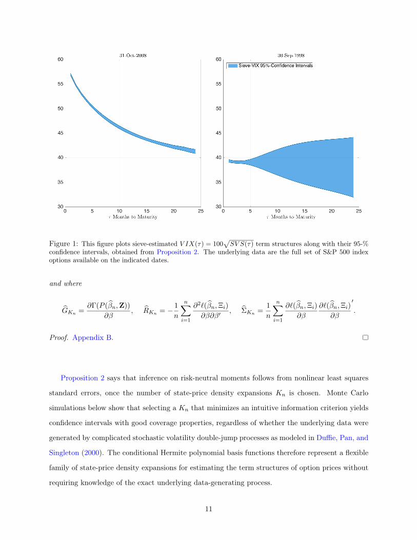
Figure 1: This figure plots sieve-estimated V IX(τ) = 100√SV S(τ) term structures along with their 95-%

confidence intervals, obtained from Proposition 2. The underlying data are the full set of S&P 500 indexoptions available on the indicated dates.

and where

GKn =∂Γ(P (βn,Z))

∂β, RKn = − 1

n

n∑i=1

∂2`(βn,Ξi)

∂β∂β′, ΣKn =

1

n

n∑i=1

∂`(βn,Ξi)

∂β

∂`(βn,Ξi)

∂β

′

.

Proof. Appendix B.

Proposition 2 says that inference on risk-neutral moments follows from nonlinear least squares

standard errors, once the number of state-price density expansions Kn is chosen. Monte Carlo

simulations below show that selecting a Kn that minimizes an intuitive information criterion yields

confidence intervals with good coverage properties, regardless of whether the underlying data were

generated by complicated stochastic volatility double-jump processes as modeled in Duffie, Pan, and

Singleton (2000). The conditional Hermite polynomial basis functions therefore represent a flexible

family of state-price density expansions for estimating the term structures of option prices without

requiring knowledge of the exact underlying data-generating process.

11

Figure 1 illustrates the resulting confidence intervals for the SV S term structure by using S&P

500 index options, converted to standard deviations in order to be directly comparable to the

familiar CBOE V IX = 100√SV S. The left panel plots the sieve-estimated VIX term structure’s

confidence intervals during the height of the 2008 financial crisis, whereas the right panel shows the

corresponding term structure confidence intervals during the height of the 1998 Russian financial

crisis and Long-Term Capital Management bailout. The figure shows that precise inferences about

risk-neutral expectations of long-run realized variance are possible, though not always a given:

during the Russian financial crisis, for example, sampling uncertainty around long-run options

made it difficult to draw firm conclusions about the shape of the implied volatility term structure

at longer maturities. The inference result outlined in Proposition 2 therefore presents a useful

robustness check for empirical work that seeks to extract information from long-maturity options,

a subject which is undertaken below.

2.4 Interpretation: Sieve Prices as Nonparametric Black-Scholes

The sieve put option price in (12) has an intuitive interpretation. Rearranging equation (12), one

obtains

P (fK ,Z) = κe−rτΦ(d(Z))− S0e−rτ+µ(Z)eσ(Z)2/2Φ(d(Z)− σ(Z))

−Ky∑k=1

γk(B, τ)

[1√kHk−1(d(Z))φ(d(Z)) + S0e

−rτ+µ(Z)I∗k(d(Z))

]. (19)

Inspection of equation (19) shows that choosing

σ(Z) ≡ σ√τ , µ(Z) ≡ (r − q − σ2/2)τ (20)

will cause the leading term in equation (19) to become

PBS(σ,Z) ≡ κe−rτΦ(d(Z))− S0e−qτΦ(d(Z)− σ√τ),

where q is the dividend yield, and where the function d(Z) from equation (6) is now d(Z) =

(log(κ/S0)− (r− q− σ2/2)τ)/(σ√τ). The value σ is a constant in the sieve framework and can be

12

chosen to equal the implied volatility of an at-the-money option.

This is the familiar option pricing formula of Black and Scholes (1973). Therefore, the choice of

µ(Z) and σ(Z) above result in a sieve approximation with leading term given by the Black-Scholes

formula, that is,

P (fK ,Z) = PBS(σ,Z)−2Ky∑k=1

γk(B, τ)

[κe−rτ√

kHk−1(d(Z))φ(d(Z)) + S0e

−qτ−σ2τ/2I∗k(d(Z))

]. (21)

This formula can be interpreted as centering the sieve at Black-Scholes, and then supplementing

it with higher-order correction terms.10 As the sample size n increases, the number of correction

terms, Ky and Kτ , also increase, albeit at a slower rate than n.11 Thus, the more data one has, the

more complex the sieve option pricer is permitted to be relative to Black-Scholes. This intuition

also carries over to hedging, since sieve-implied Greeks will be the standard Black-Scholes Greeks

augmented with higher order correction terms that can be derived in closed-form. For brevity, this

application is illustrated in the Online Appendix. In addition to their theoretical appeal, the option

prices (19) have computational advantages for studying option-implied term structures: Since the

integrals for risk-neutral moments in (16) require a continuum of option prices, it is convenient to

have closed-form expressions for the prices in order to improve upon the speed and accuracy of

numerical integration routines.

Finally, note that if the γk(B, τ) terms for k ≥ 1 above are significantly different from zero in

the data, then we can regard this as evidence against the Black-Scholes model. In particular, it has

been well-documented that conditional distributions of asset prices contain substantial volatility,

skewness, and kurtosis that the Black-Scholes model is unable to capture. Modeling techniques

to introduce such features into the return distribution includes the addition of stochastic volatility

(Heston (1993)), as well as jumps (Bates (1996), Bates (2000), Bakshi, Cao, and Chen (1997), Duffie,

Pan, and Singleton (2000)). The simulation study in Section 3 explores how these continuous time

parametric features feed into the coefficients of the Hermite expansion and shows that an empirically

tractable number of expansion terms is quite capable of fitting the conditional distributions implied

by complicated stochastic volatility and jump specifications.10Recently, Kristensen and Mele (2011), Xiu (2011), and León, Mencía, and Sentana (2009) have employed Hermite

polynomials in a parametric option pricing setting.11Recall that the γk(B, τ) terms also contain expansions in the maturity dimension.

13

2.5 Extension to Higher Order Moments

As is clear from (16), the theory of inference in Proposition 2 generalizes to different portfolio

weights. This enables the study of risk-neutral expectations of higher order moments, as proposed

for example in Bakshi, Kapadia, and Madan (2003). To this end, we compare the SVS prices to

the prices of the cubic and quartic portfolios of Bakshi, Kapadia, and Madan (2003), defined as the

risk-neutral expectations

MOM3(τ) ≡ τ−1EQ0 [e−rτR(0, τ)3] = τ−1

∫ ∞S0

6 log (κ/S0)− 3 [log(κ/S0)]2

κ2C(Z)dκ

− τ−1∫ S0

0

6 log (S0/κ) + 3 [log(S0/κ)]2

κ2P (Z)dκ

MOM4(τ) ≡ τ−1EQ0 [e−rτR(0, τ)4] = τ−1

∫ ∞S0

12 [log (κ/S0)]2 − 4 [log(κ/S0)]

3

κ2C(Z)dκ

+ τ−1∫ S0

0

12 [log (S0/κ)]2 + 4 [log(S0/κ)]3

κ2P (Z)dκ

(22)

where R(0, τ) ≡ log(Sτ/S0). Note that these moments clearly fall into the class of option spanning

portfolios covered by (16).

The VIX, cubic, and quartic portfolio term structures are plotted in Figure 2, which shows

how the they evolve over time, with red shading indicating term structures with short maturi-

ties of 1, 2, 3, . . . months, and blue shading indicating term structures with long maturities of

. . . , 22, 23, 24 months. The top panel illustrates that the volatility term structure embedded in

options is highly time varying in level and slope. While the level of the term structure moves strongly

with the familiar 1-month VIX, the slope shows occasional signs of inversion: In times when the

overall term structure level is high, short-run volatility peaks above long-run volatility, showing

that index options price in a volatility mean reversion. In most periods, however, the volatility

term structure appears upward sloping. In contrast, the cubic and quartic portfolios do not reveal

such term structure inversions, suggesting that in all periods, long-run options are pricing in more

skewness and kurtosis than short-run options.12

12Note that this effect is not mechanically due to a lengthening of maturity, as the moments in (22) are scaled bymaturity.

14

Figure 2: This figure plots the time series of estimated risk-neutral volatil-ity, cubic, and quartic term structures. Each figure plots 24 time series,representing term structures that cover 1 to 24 months. The sample periodis 1996 to 2013.

15

In level terms, the cubic and quartic portfolios in Figure 2 reveal that the strongest negative

skewness and positive kurtosis effects by far occur in crisis periods, which is also when the volatility

term structure is at its highest level. This suggests a factor structure across all three portfolios

and maturities. In fact, the first principal component of the volatility, cubic, and quartic 24-month

term structures explains 95% of their combined time series variation (Table 2). For reference, the

one-month VIX has a correlation of 80% to this principal component, whereas the one-month cubic

and quartic portfolios have correlations of -84% and 80%. But while the one-month VIX, cubic,

and quartic portfolios are all strongly related to the first principal component across all portfolios

and maturities, the second principal component is most closely related to the VIX’s term spread,

defined as the difference between 24-month VIX and 1-month VIX, V IX(24)− V IX(1). The VIX

term spread’s correlation to the second principal component is 70%, whereas the cubic and quartic

term spreads are only weakly related to the second principal component.

Table 2: Principal Components of Volatility, Cubic, and Quartic Term Structures

PC Corr to PC Corr to PC Corr toVariation VIX Level and MOM3 Level and MOM4 Level andExplained Term Spread Term Spread Term Spread

PC1 0.95 0.80 -0.84 0.80PC2 0.03 0.70 -0.29 0.22

Notes: The principal components of the combined VIX, cubic (MOM3), and quartic (MOM4) 24-monthportfolio term structures are extracted. The first column reports the variation explained by the first twoprincipal components PC1 and PC2. The remaining columns report the correlation of PC1 with level, givenby VIX(1), MOM3(1), and MOM4(1), and correlations of PC2 with term spreads, given by [V IX(24) −V IX(1)], [MOM3(24)−MOM3(1)], and [MOM4(24)−MOM4(1)].

While Figure 2 shows the point estimates of the term structures over time, Figure 3 examines how

precisely they are estimated according to the inference theory in Proposition 2. The term structures

are averaged according to a pre-financial crisis subperiod (1996-2006), when the index options were

less liquid, to a crisis subperiod (2007-2009) when the volatility term structure was often inverted,

and a post-crisis period (2010-2013), when options in the sample were at their most liquid. The

figure shows that in general, higher moment spanning portfolios are less precisely estimated when

considering the confidence interval width relative to the estimated level. For example, over the

1996-2006 period, the cubic portfolio is clearly downward sloping and negative as a point estimate.

16

Figure 3: This figure plots average risk-neutral term structures and 95% confidence intervals as introducedin Proposition 2.

However, at long maturities, this measure of skewness is no longer statistically distinguishable from

zero. In contrast, the volatility term structure appears the most precisely estimated as a fraction of

the estimated level, and that its shape in general cannot be attributed to estimation error. Finally, of

particular note is that the quartic portfolios are very imprecisely estimated, which calls into question

their use in empirical work. For example, the width of these confidence intervals may explain why

the asset pricing implications of the kurtosis portfolios in Conrad, Dittmar, and Ghysels (2013) were

relatively weaker than those obtained from the variance and skewness portfolios.

Taken together, these results suggest that the risk-neutral variance term structure is both more

precisely estimated and also captures a substantial portion of the time-series variation in higher-

17

order moments, motivating in part a focus on variance term structures below.

3 Simulations

Despite its parametric appearance, the sieve is still model-free in the sense that it can fit option

prices from a variety of unknown data generating processes (DGPs). To illustrate, this section

presents simulations of empirically realistic option price data from DGPs of varying complexity,

from which VIX term structures and confidence intervals are computed. Within the simulations,

while the researcher observes the DGP and consequently the true VIX term structure, the sieve

does not. Instead, the sieve must estimate the VIX from a finite sample of noisy option prices. In

doing so, the sieve is only permitted to vary the number of expansion terms Kn in a data-dependent

manner, making the choice of Kn as important as the choice of a bandwidth in a kernel regression.

A data-driven method for choosing Kn is proposed below and is shown to perform well across several

DGPs.

The simulations in this section refer to various subcases of the following general data generating

process,

dXt =

(r − q − λµ− 1

2Vt

)dt+ ρ

√VtdWt + JtdNt

dVt = κv(V − Vt)dt+ ρv√VtdWt +

(1− ρ2

)1/2v√VtdW

′t + ZtdNt

(23)

where Vt is a stochastic volatility process, Xt is the underlying’s log price, Wt and W ′t are standard

Brownian motions, and κv, V , ρ, v parametrize the volatility process’ mean reversion, long-run

mean, the leverage effect, and the volatility of volatility, respectively. Nt is a Poisson process with

arrival intensity λ and compensator λµ, where µ = exp(µJ + 0.5σ2J)/(1 − µv − ρJµv) − 1. The

variable Jt|Zt ∼ N(µJ + ρJZt, σ2J) is the price jump component and Zt ∼ exp(µv) is the volatility

jump component. This is the well-known stochastic volatility double-jump process (SVJJ), which

is a special case of the general affine-jump diffusion processes treated in Duffie, Pan, and Singleton

(2000) that is nonetheless general enough to nest the seminal models of Black and Scholes (1973),

Heston (1993), and other jump-diffusions commonly used in the option pricing literature. The values

of these parameters are set to those used in Andersen, Fusari, and Todorov (2012) and are given in

18

Black-Scholes Heston SVJ SVJJ

V0 0.014 0.014 0.014 0.014κ 4.032 4.032 4.032V 0.014 0.014 0.014ρ -0.460 -0.460 -0.460v 0.200 0.200 0.200λ 1.008 1.008µJ -0.050 -0.050σJ 0.075 0.075µv 0.100ρJ -0.500

Table 3: Parameter values used in the simulation exercises in Section 3.

Table 3.

Given the parameter values in Table 3, a dataset with empirically realistic options is simulated by

mimicking features of September 23, 1998, the bailout date of LTCM. This date is chosen to represent

crisis conditions while keeping the option dataset computationally manageable, due to the many

optimizations that need to be solved across all Monte Carlo datasets. That is, options are simulated

with 1, 2, 3, 6, 9, 12, 15, 21 months-to-maturity and with respective number of observations 32,

20, 44, 31, 30, 9, 23, 27. The range of strikes simulated at each maturity corresponds to the same

moneyness of options observed in the data. Finally, each drawn option price is perturbed with

uniformly distributed noise corresponding to the width of the bid-ask spread observed in the actual

data. In this way, 1000 option datasets are simulated from the SVJJ process in (23), and for each

dataset, the true VIX term structure (free of noise, discretization, and truncation error) is computed.

Furthermore, for each finite simulated sample observed with noise, the sieve least squares regres-

sion (14) is estimated. The number of sieve expansion terms Kn are chosen with both theoretical

and computational considerations in mind. While Coppejans and Gallant (2002) have shown that

leave-one-out and hold-out cross-validations perform well for univariate Hermite series in the context

of density estimations, these cross-validations typically involve heavy computation. The curse of

dimensionality compounds the problem for the two-dimensional Hermite polynomials studied here.

For example, for a sample of size n, leave-one-out cross validation requires computation of the non-

linear regression (14) (n−1) times for many configurations of Kn = (Ky(n)+1)(Kτ (n)+1). Among

computationally feasible selection criteria, minimizing the Bayesian Information Criterion (BIC) or

19

Table 4: Monte Carlo Rejection Frequencies.

Maturity (months) ExpansionsDGP 1 2 3 6 9 12 15 21 (Ky,Kτ )

SVJJ 0.051 0.020 0.030 0.020 0.030 0.030 0.020 0.010 (7,2)SVJ 0.003 0.027 0.038 0.034 0.044 0.022 0.041 0.050 (6,2)Heston 0.034 0.018 0.018 0.020 0.030 0.049 0.087 0.078 (4,2)Black-Scholes 0.035 0.036 0.026 0.018 0.031 0.043 0.052 0.046 (0,0)

Notes: A dense surface of true option prices was simulated under an SVJJ specification for each of the maturitiesshown, from which a true VIX was computed without moneyness truncation error. Then, 1000 random subsampleswere drawn from this surface. These sample prices were perturbed with a uniformly distributed error corresponding tothe width of observed bid-ask spreads on S&P 500 index options. V IX(τ) estimates were computed and studentizedaccording to Proposition 2, and corresponding 95% confidence intervals were constructed by inverting nominal level5% tests. Rejection frequencies report the proportion of simulated draws for which the true V IX(τ) was outside the95% confidence intervals.

the well-known Mallows (1973) criterion, which is asymptotically equivalent to leave-one-out cross-

validation in certain settings, are natural candidates that perform equally well in the simulations

studied in this paper.13

At each Monte Carlo iteration, the result of the sieve least squares regression are closed-form

option prices P (Z) ≡ P (β,Z) (derived in Proposition 1), which can be computed with arbitrarily

dense strikes for any given maturity. These prices are then fed into the integral in (1), which

is computed at each observed maturity. Because the sieve estimates allow extrapolations into

the strike tails, it is possible to set the strike integration range in a manner that ensures that

prices representing the 0.5% to 99.5% quantiles of the implied risk-neutral distribution are included,

allowing the sieve to substantially reduce strike truncation errors. Finally, following Proposition 2,

the studentized V IX(τ) curve is computed for each simulated dataset, and the corresponding 95%

confidence intervals are formed using standard normal critical values.

Table 4 shows the rejection frequencies of the inference procedure, i.e. the proportion of datasets

for which the the 95% confidence intervals do not cover the true VIX at each maturity along the

term structure. The results show that for the nominal level 5% test considered, the confidence

intervals display good, though often slightly conservative, size control. The right-most column,

which shows the modal number of expansion terms that were selected by the aforementioned data-13Mallows (1973) criterion involves solving

Kn = arg minK

1

n

n∑i=1

[Pi − P (βK ,Zi)

]2W (Zi) + 2σ2(K/n).

See also Li and Racine (2007, p. 451).

20

driven procedure, suggests a clear relationship between the complexity of the underlying DGP and

the number of expansions K = (Ky + 1)(Kτ + 1) selected. Importantly, when the underlying DGP

is in fact Black-Scholes, the modal number of expansions chosen was the correct (0, 0).

Finally, notice that while the sieve state-price densities f(Y |τ) do not explicitly depend on

stochastic volatility, the sieve nonetheless performs well in capturing the option-implied term struc-

tures of stochastic processes that do allow for stochastic volatility. This is because the effect of

stochastic volatility (as well as jumps) is to create option prices whose underlying state-price den-

sities are different by maturity. Hence, stochastic volatility and jumps can be viewed as modeling

devices that uncouple long-run option prices from short-run option prices. The sieve captures this

effect directly by allowing long-maturity state-price densities to differ from their short-maturity

counterparts. The sieve’s effectiveness in doing so is explored in further simulations in the Online

Appendix C.

4 Return Predictability in the Term Structure of Variance Risk

Premia

This section combines the sieve framework with a novel set of expectation hypothesis and return

predictability regressions to study the term structure of the variance risk premium and its link to

equity risk premia. Following Bollerslev, Tauchen, and Zhou (2009), the variance risk premium is

defined as follows. Let realized variance from month t to T = t+ τ be given by the annualized sum

of squared daily returns

RVt,T ≡252

n

n∑i=1

(sp500(t+ i∆n)− sp500(t+ (i− 1)∆n)

sp500(t+ (i− 1)∆n)

)2

, (24)

where n = τ/∆n is the number of trading days between t and T , ∆n is the daily increment, and

sp500(t) represents the level of the S&P 500 index at time t. The variance risk premium is the

difference between objective (P-measure) and risk-neutral (Q-measure) conditional expectations of

RVt,T

V RPt(t, T ) ≡ EPt [RVt,T ]− EQ

t [RVt,T ]. (25)

21

Note that for a pricing kernel Mt,T and mt,T ≡Mt,T /EPt [Mt,T ],

EQt [RVt,T ] = EP

t [mt,TRVt,T ] = EPt [RVt,T ] + CovPt [mt,T , RVt,T ],

so that the difference in (25) measures covariation of realized variance with the pricing kernel, or in

other words, a risk premium. Following Carr and Wu (2009), the quantity EQt [RVt,T ] is well repli-

cated by the synthetic variance swap, i.e. the integrated option portfolio (1): SV St(τ) = EQt [RVt,T ]

up to a third-order approximation error.

Expectation Hypothesis Under a null hypothesis H0 : CovPt [mt,T , RVt,T ] = 0 of no vari-

ance risk premium, one has EQt [RVt,T ] = EP

t [RVt,T ], so that for εt+τ with EPt [εt+τ ] = 0, RVt,T =

EQt [RVt,T ] + εt+τ . Therefore, H0 is equivalent to the joint null hypothesis a = 0 and b = 1 in the

regressions

RVt,T = a(τ) + b(τ)EQt [RVt,T ] + εt+τ . (26)

The idea is to test several hypotheses of this form and to relate them to well-established findings

for the 1-month VRP. We therefore augment (26) with the concept of a forward variance, which

takes advantage of the additive properties of RVt,T : Note that from (24), one has for horizons τ > 1,

RVt,T = RVt,t+1 +RVt+1,T , giving rise to a decomposition

V RPt(t, T ) = EPt [RVt,t+1 +RVt+1,T ]− EQ

t [RVt,t+1 +RVt+1,T ]

= EPt [RVt,t+1]− EQ

t [RVt,t+1] + EPt [RVt+1,T ]− EQ

t [RVt+1,T ]

≡ V RPt(t, t+ 1) + V RPt(t+ 1, T ).

(27)

Notice that the first component on the right-hand side is the familiar one-month variance risk

premium that has been extensively studied in the literature using published (one-month) VIX

data.14 Therefore, in order to relate findings on V RPt(t, T ) to our existing understanding of the

1-month variance risk premium, we also test hypotheses regarding the forward variance risk premium

RVt+1,T = a(τ) + b(τ)EQt [RVt+1,T ] + εt+τ , (28)

14See, for example, Carr and Wu (2009), Bollerslev and Todorov (2011), Bollerslev, Gibson, and Zhou (2011),Drechsler and Yaron (2011), Bollerslev, Osterrieder, Sizova, and Tauchen (2013), Bekaert and Hoerova (2014).

22

where EQt [RVt+1,T ] = [SV St(τ) − SV St(1)] captures the steepness of the synthetic variance swap

curve in maturity. A test of H0 : a = 0 ∩ b = 1 is a test of the forward variance risk premium

V RPt(t+ 1, T ).

Return Predictability Bollerslev, Tauchen, and Zhou (2009) and Bekaert and Hoerova

(2014), among others, provide evidence that V RPt(t, t + 1) predicts excess stock market returns.

Using the sieve-estimated term structure of SV St(τ), one can test whether their predictability result

extends to long-run variance risk premia as well as forward variance risk premia, i.e. V RPt(t, T )

and V RPt(t+ 1, T ). We therefore estimate both

Ret+h = αh,τ + βh,τV RPt(t, T ) + εt+h and

Ret+h = αh,τ + βh,τV RPt(t, t+ 1) + γh,τV RPt(t+ 1, T ) + εt+h

(29)

for various forecasting horizons h and term structure maturities τ , where Ret+h denotes the h-month

ahead CRSP value-weighted return (including dividends) in excess of the risk-free rate. To ensure

that V RPt(t, T ) = EPt [RVt,T ] − EQ

t [RVt,T ] lies in the time t information set, we need a P-measure

forecast of realized variance, EPt [RVt,T ], which we obtain from the standard heterogeneous AR model

of Corsi (2009),

RVt,t+1 = b0 + b1RVt + b2

(1

6

5∑i=0

RVt−i

)+ b3

(1

24

23∑i=0

RVt−i

)+ εt+1, (30)

which effectively captures the long-memory dynamics of the RVt process. To avoid look-ahead bias,

(30) is estimated for each month t in our option sample 1996-2013, using monthly S&P 500 index

RV (24) from 1950 to t. The results and conclusions below do not materially depend on the exact

lag structure of this RV forecasting regression, since they are upheld under various specifications.

Long-run forecasts of RVt,T can be obtained by iterating (30) forward.

4.1 S&P 500 Index Option Data

To run the regressions in (26), (28), and (29), we use the proposed sieve framework to estimate a

balanced monthly time series of SV St(τ) = EQt [RVt,T ] term structures from data on S&P 500 index

options (SPX) spanning January, 1996 to August, 2013. Following the data filtering procedure of

23

Andersen, Fusari, and Todorov (2012), we use the average of closing bid and ask quotes, discard all

in-the-money options, and options with maturities of less than 7 days. Call option information is

incorporated by converting out-of-the-money calls to in-the-money puts by put-call parity. Further-

more, we follow the CBOE (2003) VIX White Paper procedure of excluding options with strikes

beyond the first pair of zero-bid option prices. Table 1 presents summary statistics of the resulting

dataset, which includes option surfaces observed at the end of the month, for a total of 212 months.

To be specific, for each month t of these 212 option cross-sections, we solve the sieve least squares

problem (14) and compute the portfolio integration in (1) for τ = 1, 2, . . . , 24 months-to-maturity.

At each of these maturities, the integration limits in (1) were set to cover the 0.5% to 99.5% quantiles

of the implied risk-neutral CDF, yielding a balanced monthly term structure SV St(τ). To check that

the resulting SV St(τ) produces coherent estimates of implied volatility at the one-month horizon,

we plot 100 · SV St(1)1/2 = V IXt(1) against the CBOE’s published VIX in the top panel of Figure

4. The unconditional correlation between the two series is 0.9976, and the number of expansion

terms selected via the data-driven criterion (Section 3) was about (Ky,Kτ ) = (8, 3) on average.

Finally, note that inference on regressions of the form (26) and (28) can be affected by mea-

surement error and persistence in the regressors. Measurement error in the regressors is known

to cause attenuation bias in the slope coefficient, which is especially problematic when testing

hypotheses of the form b = 1. That is, by replacing EQt [RVt,T ] in equation (26) with its esti-

mate SV St(τ) = EQt [RVt,T ] + ηt,T , one obtains RVt,T = α(τ) + β(τ)SV St(τ) + ut+τ = α(τ) +

β(τ)[EQt [RVt,T ] + ηt,T ] + ut+τ . Assuming for simplicity that each ηt,T is independent of other

variables, we see from standard arguments that β(τ) = Cov(RVt,T , SV St(τ))/V ar[SV St(τ)] =

b(τ)V ar[EQt [RVt,T ]]/V ar[EQ

t [RVt,T ]] + E[σ2η,t] ≡ b(τ)φ(τ), which is the classical measurement er-

ror attenuation bias. Note that Proposition 2 ensures that for fixed t,√nt(SV St(τ)−EQ

t [RVt,T ])→d

N(0, σ2η,t), and hence one can use the sieve standard errors to perform a simple bias correction by

multiplying the estimated β(τ) by an estimate of φ(τ)−1, which is greater than one. The bottom

left panel of Figure 4 plots the estimated bias correction φ(τ)−1 (in excess of one) and shows that

the bias can play a significant role (up to 14%) for long-horizon τ = 24. On average, term structure

estimation error ranges from 2% to 14% of time-series variation in the synthetic variance swap curve

(Figure 4, middle right panel). Finally, note that serial correlation in the regressors is increasing in

τ , but all cases well below 1.

24

Figure 4: Pre-regression Diagnostics. The top panel plots a comparison of the sieve-estimated 30-day VIXand the CBOE published 30-day VIX. The middle left panel plots the average 95% confidence intervals ofthe synthetic variance swap term structure. The middle right panel shows the ratio of average sieve standarderrors of SV St(τ) to the time series standard deviation of SV St(τ). The bottom left panel shows thebias correction factor (in excess of one) to be applied to the slope coefficient in the expectation hypothesisregression, and the bottom right panel plots the sample first-order autocorrelation of SV St(τ) for maturitiesτ = 1, . . . , 24. Sieve standard errors for SV St(τ) are computed for 212 months from January, 1996, toAugust, 2013, using S&P 500 index options and the inference procedure in Proposition 2.

25

4.2 Results

Expectation Hypothesis The results of the bias-corrected regressions (26) and (28) are

surprising. p-values in the first row of Table 5 show strong evidence against the null hypothesis

H0 : a = 0∩b = 1 of no variance risk premium V RPt(t, T ) across all maturities τ = 1, . . . , 12, 18, 24.

In contrast, the forward variance tests reported in the bottom panel are unable to reject the null

hypothesis of no forward variance risk premium V RPt(t+1, T ). A notable exception is at the τ = 2

horizon, whose p-value in the forward regression is smaller than in the full regression, suggesting

that investors earn a premium for being exposed to variance risk between t+ 1 and t+ 2 as well. In

sum, the strong rejections in the first row and the lack of rejection in the second row suggest that

compensation for variance risk is concentrated on the first one or two maturities.15

Table 5: p-Values for Expectation Hypothesis Regressions.

τ

1 2 3 4 5 6 7 8 9 10 11 12 18 24

SVS 0.000 0.074 0.019 0.003 0.001 0.000 0.000 0.000 0.000 0.000 0.000 0.000 0.000 0.000Forward - 0.032 0.072 0.111 0.141 0.189 0.227 0.271 0.324 0.371 0.401 0.421 0.529 0.537

Notes: The bias-corrected OLS regressions from (26) and (28) of realized variance on sieve syntheticvariance swaps SV St(τ) and forward variance swaps SV St(τ) − SV St(1), respectively, are estimated foreach of the monthly horizons τ = 1, . . . , 12, 18, 24. p-values in the first row report the outcome of the jointtests a(τ) = 0 ∩ b(τ) = 1 for the regression on the full variance swap regression (26), and the second rowshows the corresponding outcome for the forward variance swap (28). Newey and West (1987) standarderrors for lag length 24 are used.

Return Predictability The results of the expectation hypothesis tests are further corrobo-

rated in the return predictability regressions. Table 6 reports t-statistics on the slope coefficient of

the first regression in (29) using Hodrick (1992) standard errors.16 The left-most column shows the

same pattern of excess return predictability on horizons h = 2, . . . , 7 found in Bollerslev, Tauchen,

and Zhou (2009) for one-month V RPt(t, t + 1). The pattern is noteworthy given that Bollerslev,

Tauchen, and Zhou (2009) use S&P 500 index excess returns, whereas we use CRSP value-weighted

excess returns over a different sample period as the left-hand side variable. Further out into the15For reference, the full regression output is provided in the Online Appendix.16See the discussion in Ang and Bekaert (2007) in favor of using Hodrick (1992) standard errors in overlapping

return predictability regressions.

26

Table 6: Excess Return Predictability of the VRP Term Structure.

t-stat on V RPt(t, T )

h \ τ 1 2 3 4 5 6 7 8 9 10 11 12 18 24

h=1 -1.21 -1.28 -1.41 -1.53 -1.61 -1.65 -1.63 -1.59 -1.55 -1.52 -1.49 -1.47 -1.32 -1.27h=2 -2.00 -2.02 -2.12 -2.24 -2.30 -2.30 -2.24 -2.18 -2.11 -2.06 -2.01 -1.97 -1.77 -1.65h=3 -2.28 -2.17 -2.22 -2.32 -2.40 -2.41 -2.36 -2.30 -2.23 -2.18 -2.14 -2.09 -1.89 -1.71h=4 -2.03 -1.96 -2.04 -2.16 -2.26 -2.30 -2.27 -2.23 -2.19 -2.15 -2.12 -2.09 -1.93 -1.77h=5 -1.92 -1.97 -2.10 -2.24 -2.34 -2.38 -2.36 -2.32 -2.28 -2.25 -2.22 -2.18 -1.99 -1.90h=6 -2.09 -2.09 -2.17 -2.27 -2.33 -2.35 -2.33 -2.30 -2.26 -2.23 -2.20 -2.16 -1.97 -1.87h=7 -2.04 -2.03 -2.10 -2.19 -2.26 -2.28 -2.27 -2.24 -2.21 -2.18 -2.14 -2.11 -1.91 -1.76h=8 -1.75 -1.78 -1.85 -1.92 -1.97 -1.99 -1.98 -1.96 -1.94 -1.91 -1.89 -1.86 -1.67 -1.58h=9 -1.54 -1.59 -1.65 -1.71 -1.75 -1.77 -1.76 -1.75 -1.74 -1.73 -1.71 -1.70 -1.53 -1.46h=10 -1.30 -1.39 -1.47 -1.54 -1.59 -1.61 -1.62 -1.61 -1.61 -1.60 -1.59 -1.58 -1.40 -1.32h=11 -1.17 -1.27 -1.36 -1.43 -1.48 -1.51 -1.52 -1.52 -1.51 -1.50 -1.49 -1.48 -1.31 -1.21h=12 -1.10 -1.18 -1.25 -1.31 -1.35 -1.37 -1.37 -1.36 -1.35 -1.34 -1.33 -1.32 -1.15 -1.08

t-stat on forward V RPt(t+ 1, T )

h \ τ 1 2 3 4 5 6 7 8 9 10 11 12 18 24

h=1 0.18 0.01 -0.10 -0.14 -0.15 -0.11 -0.08 -0.04 -0.01 0.01 0.02 0.13 0.19h=2 0.23 0.01 -0.15 -0.20 -0.19 -0.13 -0.09 -0.05 -0.02 -0.00 0.02 0.16 0.24h=3 0.66 0.35 0.04 -0.14 -0.22 -0.22 -0.20 -0.18 -0.16 -0.14 -0.13 -0.00 0.15h=4 0.17 -0.13 -0.40 -0.57 -0.65 -0.65 -0.63 -0.61 -0.60 -0.58 -0.57 -0.45 -0.31h=5 -0.66 -0.93 -1.10 -1.18 -1.20 -1.16 -1.12 -1.08 -1.04 -1.01 -0.97 -0.78 -0.70h=6 -0.65 -0.85 -1.00 -1.07 -1.10 -1.08 -1.05 -1.02 -1.00 -0.97 -0.94 -0.74 -0.65h=7 -0.72 -0.88 -1.01 -1.08 -1.11 -1.10 -1.08 -1.05 -1.02 -0.99 -0.96 -0.74 -0.60h=8 -0.81 -0.93 -1.02 -1.06 -1.07 -1.06 -1.04 -1.01 -0.98 -0.96 -0.93 -0.71 -0.62h=9 -0.83 -0.90 -0.95 -0.97 -0.98 -0.97 -0.96 -0.94 -0.93 -0.92 -0.90 -0.71 -0.65h=10 -0.96 -1.02 -1.05 -1.05 -1.04 -1.02 -1.01 -0.99 -0.97 -0.95 -0.94 -0.72 -0.64h=11 -1.03 -1.09 -1.10 -1.09 -1.07 -1.04 -1.02 -0.99 -0.97 -0.95 -0.94 -0.72 -0.61h=12 -0.86 -0.91 -0.92 -0.90 -0.88 -0.86 -0.84 -0.81 -0.79 -0.78 -0.76 -0.56 -0.50

Notes: The top panel reports Hodrick (1992) t-statistics from regressions of monthly CRSP value-weightedexcess returns on the lagged term structure of variance risk premia (29), i.e. Ret+h = αh,τ+βh,τV RPt(t, T )+εt+h, where T = t + τ .The bottom panel reports analogous t-statistics for regressions of excess returns onlagged forward variance risk premia Ret+h = αh,τ + γh,τV RPt(t + 1, T ) + εt+h. The forward variance riskpremia reflect compensation for volatility occurring over month t+1 to T . Gray shading denotes significanceat the 5% level..

term structure, the remaining columns of Table 6 show that the strong predictive pattern is mir-

rored for V RPt(t, T ) for τ = 2, . . . , 12. Note that the negative sign on the t-statistics indicates

that declines in the variance risk premium (e.g. P-measure forecasts of volatility exceed Q-measure

implied volatility) tend to predict positive excess returns. Heuristically, the sign is consistent with

the intuition that long positions in variance swaps are often used as hedges against high-marginal

utility states, since they pay out when realized variance exceeds implied variance.

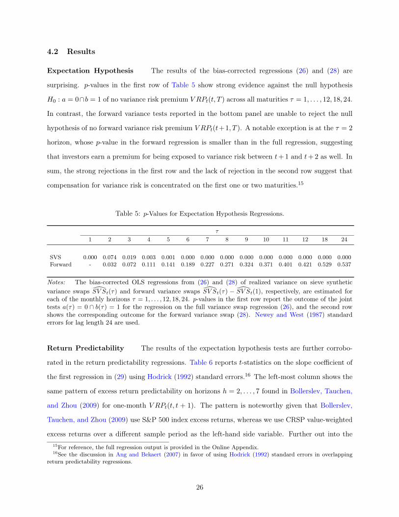
One implication of excess return predictability is that it provides a measure for the time-variation

of the equity risk premium, Et[Ret+h] = αh,τ + βh,τV RPt(t, t+ τ). Figure 5 illustrates examples for

the 6-month ahead equity risk premium using the slower-moving 6,12,18, and 24-month variance risk

27

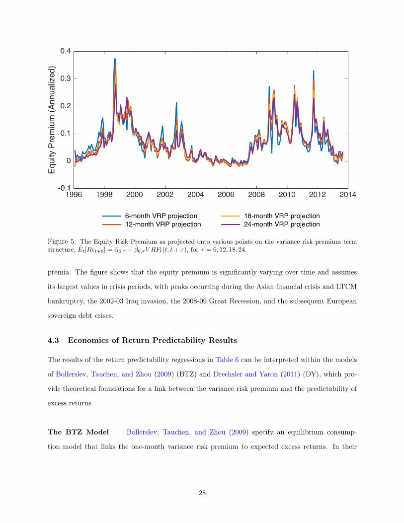
Figure 5: The Equity Risk Premium as projected onto various points on the variance risk premium termstructure, Et[Ret+6] = α6,τ + β6,τV RPt(t, t+ τ), for τ = 6, 12, 18, 24.

premia. The figure shows that the equity premium is significantly varying over time and assumes

its largest values in crisis periods, with peaks occurring during the Asian financial crisis and LTCM

bankruptcy, the 2002-03 Iraq invasion, the 2008-09 Great Recession, and the subsequent European

sovereign debt crises.

4.3 Economics of Return Predictability Results

The results of the return predictability regressions in Table 6 can be interpreted within the models

of Bollerslev, Tauchen, and Zhou (2009) (BTZ) and Drechsler and Yaron (2011) (DY), which pro-

vide theoretical foundations for a link between the variance risk premium and the predictability of

excess returns.

The BTZ Model Bollerslev, Tauchen, and Zhou (2009) specify an equilibrium consump-

tion model that links the one-month variance risk premium to expected excess returns. In their

28

model, consumption growth gt+1 = log(Ct+1/Ct) follows

gt+1 = µg + σg,tzg,t+1, (31)

where zg,t+1 is i.i.d. N(0, 1). The consumption volatility dynamics are governed by mean-reverting

square root processes

σg,t+1 = aσ + ρσσ2g,t +

√qtzσ,t+1, (32)

qt+1 = aq + ρqqt + φq√qtzq,t+1, (33)

where zσ,t+1 and zq,t+1 are i.i.d. N(0, 1) innovations, and where the parameters satisfy certain

regularity conditions. The process qt represents the volatility of consumption volatility, which is

itself stochastic. The main implication of the Bollerslev, Tauchen, and Zhou (2009) is that under

Epstein and Zin (1991) recursive preferences, the variance risk premium for returns on the economy’s

consumption asset is given by

EPt

[σ2r,t+1

]− EQ

t

[σ2r,t+1

]= const.× qt, (34)

where const. is a constant scalar consisting of sums and products of the model’s fundamental

parameters. Equation (34) says that in the Bollerslev, Tauchen, and Zhou (2009) economy, time-

variation in the variance risk premium is driven entirely by the single consumption vol-of-vol process

qt.

It is straightforward to show that the entire term structure of variance risk premia in this econ-

omy, EPt

[σ2r,t+j

]− EQ

t

[σ2r,t+j

]for j > 1, is also linearly driven by the same consumption vol-of-vol

process qt, as are the economy’s forward VRPs. Thus an implication of the Bollerslev, Tauchen, and

Zhou (2009) is that forward variance risk premia must also predict returns, a result that is strongly

at odds with the bottom panel of Table 6. Instead, the results of Table 6 suggest a model in which

at least two factors drive time-variation in the term structure of the variance risk premium, with

the first factor driving short-run VRP having the ability to predict excess returns, and the second

factor driving forward VRP, which does not have predictive content. Furthermore, note that the

second factor may not simply be white noise, since the top panel of Table 6 suggests that the sum

29

of short-run VRP and forward VRP still predict excess returns.

The DY Model Similar implications are readily obtained from the Drechsler and Yaron

(2011) model. The state vector in their long-run risk economy with recursive preferences is given

by Yt ∈ Rn, which follows a VAR

Yt+1 = µ+ FYt +Gtzt+1 + Jt+1, (35)

whose shocks are driven by both Gaussian innovations zt+1 ∼ N(0, In) and a Poisson jump process

Jt+1. The state vector of main interest is Yt+1 = (gt+1, xt+1, σ2t+1, σ

2t+1,∆dt+1), where xt+1 is the

persistent conditional mean of consumption growth gt+1, where σ2t+1 drives stochastic volatility

across the state vector (GtG′t = h + Hσσ2t ), σ2t+1 is the long-run mean of volatility, and ∆dt+1 is

dividend growth.

The key state variable that emerges from the Drechsler and Yaron (2011) model is σ2t , which

drives time variation in both the variance risk premium as well as the equity risk premium. How-

ever, Drechsler and Yaron (2011) show that forward VRP (the drift difference of VRP in their

terminology) is also driven by an affine function of σ2t whose intercept and coefficients depend on

model fundamentals. Hence in the Drechsler and Yaron (2011) economy, forward VRP also predicts

excess returns, which is at odds with the findings in the bottom panel of Table 6.

Broader Implications The results of this exercise suggests a link between the term structure

of variance risk premia (as considered in Dew-Becker, Giglio, Le, and Rodriguez (2015), Andries,

Eisenbach, Schmalz, and Wang (2015), and Aït-Sahalia, Karaman, and Mancini (2015) and the

equity term structure (van Binsbergen, Brandt, and Koijen (2012)). In particular, van Binsbergen,

Brandt, and Koijen (2012) show that the equity premium is closely tied to discount rates of short-

term dividend cash flows. Analogously, the above return predictability exercise shows that only

discount rates of short-run variance cash flows have implications for the equity premium. Taken

together, these results appear to connect the discount rates of short-term variance cash flows to

those of short-run equity cash flows, which in turn has implications for the joint modeling of equity

and variance risk premia.

30

5 Conclusion

This paper developed a methodological framework for measuring long-run risk-neutral expectations

of variance and other moments from options. By constructing sieve approximations to the term

structure of state-price densities, the paper derives new closed-form option prices that can be inter-

preted as nonparametric extensions of the Black-Scholes formula. The sieve approximations involve

basis function expansions that grow slowly with the sample size and can fit a variety of unknown

DGPs, as confirmed in a simulation exercise. The methodological framework suggests future lines

of research that explore option-implied term structures in the cross-section. In particular, to the

extent that options written on individual stocks, industry ETFs, and even fixed-income instruments

like swaps are less liquid than the S&P 500 index options considered above, the nonparametric con-

fidence intervals provided in this paper provide a useful metric with which to compare the precision

of option spanning portfolios across assets and asset classes.

The paper’s main empirical application concerns the term structure of variance risk premia.

Using the sieve’s estimates of risk-neutral implied variance, the paper presents new findings on the

relationship between variance risk premia and equity market return predictability. In particular, a

decomposition of the variance risk premium into a short-run component and a forward risk premium

suggests that only the short-run component predicts excess returns. This finding is at odds with

existing asset pricing models that seek to explain the variance risk premium’s predictive content,

since these models counterfactually imply that the forward variance risk premium should also predict

excess returns. Hence information contained in the term structure of risk-neutral variance provides

an alternative benchmark against which to test existing asset pricing theories. The results therefore

suggest future directions for expanding existing equilibrium models of the variance risk premium

and return predictability to account for term structure effects.

31

References

Adams, R. A., and J. J. Fournier (2003): Sobolev spaces, vol. 140. Access Online via Elsevier.

Aït-Sahalia, Y., and J. Duarte (2003): “Nonparametric option pricing under shape restrictions,”Journal of Econometrics, 116(1), 9–47.

Aït-Sahalia, Y., M. Karaman, and L. Mancini (2015): “The Term Structure of VarianceSwaps, Risk Premia, and the Expectation Hypothesis,” Available at SSRN 2136820.

Aït-Sahalia, Y., and A. W. Lo (1998): “Nonparametric estimation of state-price densities im-plicit in financial asset prices,” The Journal of Finance, 53(2), 499–547.

Andersen, T. G., N. Fusari, and V. Todorov (2012): “Parametric inference and dynamicstate recovery from option panels,” Discussion paper, National Bureau of Economic Research.

Andries, M., T. Eisenbach, M. Schmalz, and Y. Wang (2015): “The term structure of theprice of variance risk,” Discussion paper, Working Paper.

Ang, A., and G. Bekaert (2007): “Stock return predictability: Is it there?,” Review of FinancialStudies, 20(3), 651–707.

Bakshi, G., C. Cao, and Z. Chen (1997): “Empirical performance of alternative option pricingmodels,” The Journal of Finance, 52(5), 2003–2049.

Bakshi, G., N. Kapadia, and D. Madan (2003): “Stock return characteristics, skew laws, andthe differential pricing of individual equity options,” Review of Financial Studies, 16(1), 101–143.

Bakshi, G., and D. Madan (2000): “Spanning and derivative-security valuation,” Journal ofFinancial Economics, 55(2), 205–238.

Bansal, R., and A. Yaron (2004): “Risks for the long run: A potential resolution of asset pricingpuzzles,” The Journal of Finance, 59(4), 1481–1509.

Bates, D. (1996): “Jumps and stochastic volatility: Exchange rate processes implicit in DeutscheMark options,” Review of financial studies, 9(1), 69–107.

(2000): “Post-’87 crash fears in the S&P 500 futures option market,” Journal of Econo-metrics, 94(1-2), 181–238.

Bekaert, G., and M. Hoerova (2014): “The VIX, the variance premium and stock marketvolatility,” Journal of Econometrics, forthcoming.

Billingsley, P. (1995): “Probability and measure. 1995,” John Wiley&Sons, New York.

Black, F., and M. Scholes (1973): “The pricing of options and corporate liabilities,” The Journalof Political Economy, pp. 637–654.

Bollerslev, T., M. Gibson, and H. Zhou (2011): “Dynamic estimation of volatility risk premiaand investor risk aversion from option-implied and realized volatilities,” Journal of Econometrics,160(1), 235–245.

Bollerslev, T., D. Osterrieder, N. Sizova, and G. Tauchen (2013): “Risk and return:Long-run relations, fractional cointegration, and return predictability,” Journal of Financial Eco-nomics, 108(2), 409–424.

32

Bollerslev, T., G. Tauchen, and H. Zhou (2009): “Expected stock returns and variance riskpremia,” Review of Financial Studies, 22(11), 4463–4492.

Bollerslev, T., and V. Todorov (2011): “Tails, fears, and risk premia,” The Journal of Finance,66(6), 2165–2211.

Bondarenko, O. (2003): “Estimation of risk-neutral densities using positive convolution approx-imation,” Journal of Econometrics, 116(1), 85–112.

Campbell, J., and J. Cochrane (1999): “By Force of Habit: A Consumption-Based Explanationof Aggregate Stock Market Behavior,” The Journal of Political Economy, 107(2), 205–251.

Carr, P., and L. Wu (2009): “Variance risk premiums,” Review of Financial Studies, 22(3),1311–1341.

CBOE (2003): “The CBOE Volatility Index - VIX White Paper,” URL:http://www.cboe.com/micro/vix/vixwhite.pdf.

Chen, X. (2007): “Large sample sieve estimation of semi-nonparametric models,” Handbook ofEconometrics, 6, 5549–5632.

Chen, X., Z. Liao, and Y. Sun (2014): “Sieve inference on possibly misspecified semi-nonparametric time series models,” Journal of Econometrics, 178, 639–658.

Chen, X., and X. Shen (1998): “Sieve extremum estimates for weakly dependent data,” Econo-metrica, pp. 289–314.

Christoffersen, P., M. Fournier, and K. Jacobs (2013): “The Factor Structure in EquityOption Prices,” .

Conrad, J., R. F. Dittmar, and E. Ghysels (2013): “Ex ante skewness and expected stockreturns,” The Journal of Finance, 68(1), 85–124.

Coppejans, M., and A. R. Gallant (2002): “Cross-validated SNP density estimates,” Journalof Econometrics, 110(1), 27–65.

Corsi, F. (2009): “A simple approximate long-memory model of realized volatility,” Journal ofFinancial Econometrics, 7(2), 174–196.

Dew-Becker, I., S. Giglio, A. Le, and M. Rodriguez (2015): “The price of variance risk,”Discussion paper, National Bureau of Economic Research.

Drechsler, I., and A. Yaron (2011): “What’s vol got to do with it,” Review of Financial Studies,24(1), 1–45.

Driessen, J., P. J. Maenhout, and G. Vilkov (2009): “The price of correlation risk: Evidencefrom equity options,” The Journal of Finance, 64(3), 1377–1406.

Duffie, D., J. Pan, and K. Singleton (2000): “Transform analysis and asset pricing for affinejump-diffusions,” Econometrica, 68(6), 1343–1376.

Epstein, L. G., and S. E. Zin (1991): “Substitution, risk aversion, and the temporal behavior ofconsumption and asset returns: An empirical analysis,” Journal of political Economy, pp. 263–286.

33

Fackler, P. L. (2005): “Notes on matrix calculus,” North Carolina State University.

Figlewski, S. (2008): “Estimating the Implied Risk Neutral Density,” Volatility and Time SeriesEconometrics: Essay in Honor of Robert F. Engle. Editors: Tim Bollerslev, Jeffrey R. Russell,Mark Watson, Oxford, UK: Oxford University Press.

Gallant, A. R., and D. W. Nychka (1987): “Semi-nonparametric maximum likelihood estima-tion,” Econometrica: Journal of the Econometric Society, pp. 363–390.

Heston, S. (1993): “A closed-form solution for options with stochastic volatility with applicationsto bond and currency options,” Review of financial studies, 6(2), 327–343.

Hodrick, R. J. (1992): “Dividend yields and expected stock returns: Alternative procedures forinference and measurement,” Review of Financial studies, 5(3), 357–386.

Jiang, G., and Y. Tian (2005): “The model-free implied volatility and its information content,”Review of Financial Studies, 18(4), 1305–1342.

Kristensen, D., and A. Mele (2011): “Adding and subtracting Black-Scholes: a new approachto approximating derivative prices in continuous-time models,” Journal of financial economics,102(2), 390–415.

León, Á., J. Mencía, and E. Sentana (2009): “Parametric properties of semi-nonparametricdistributions, with applications to option valuation,” Journal of Business & Economic Statistics,27(2), 176–192.

Leslie, R. A. (1991): “How not to repeatedly differentiate a reciprocal,” American MathematicalMonthly, pp. 732–735.

Li, Q., and J. S. Racine (2007): Nonparametric econometrics: Theory and practice. PrincetonUniversity Press.

Mallows, C. L. (1973): “Some comments on C p,” Technometrics, 15(4), 661–675.

Newey, W., and K. West (1987): “A simple, positive semi-definite, heteroskedasticity and au-tocorrelation consistent covariance matrix,” Econometrica: Journal of the Econometric Society,pp. 703–708.

Newey, W. K. (1991): “Uniform convergence in probability and stochastic equicontinuity,” Econo-metrica, 59(4), 1161–1167.

Nickl, R., and B. M. Pötscher (2007): “Bracketing metric entropy rates and empirical centrallimit theorems for function classes of Besov-and Sobolev-type,” Journal of Theoretical Probability,20(2), 177–199.

van Binsbergen, J., M. Brandt, and R. Koijen (2012): “On the Timing and Pricing ofDividends,” American Economic Review, 102(4), 1596–1618.

van Binsbergen, J., W. Hueskes, R. Koijen, and E. Vrugt (2013): “Equity yields,” Journalof Financial Economics, 110(3), 503 – 519.

Van Binsbergen, J. H., and R. S. Koijen (2015): “The Term Structure of Returns: Facts andTheory,” Available at SSRN 2597481.

34

Van De Geer, S. (2000): Empirical processes in M-estimation, vol. 45. Cambridge university pressCambridge.

Van Der Vaart, A. W., and J. A. Wellner (1996): Weak Convergence. Springer.

Xiu, D. (2011): “Dissecting and Deciphering European Option Prices using Closed-Form SeriesExpansion,” Chicago Booth Research Paper, (11-40).

Yatchew, A., and W. Härdle (2006): “Nonparametric state price density estimation usingconstrained least squares and the bootstrap,” Journal of Econometrics, 133(2), 579–599.

35

A Definitions and Preliminary Theoretical Results

A.1 Defining the Sobolev Sieve Spaces

We begin by presenting a precise definition of the sieve spaces referenced in the main paper. The final sievespaces of interest are collections of conditional densities that we obtain by first defining a space of jointdensities, and whose future payoff component can be integrated out to yield marginals. As mentioned above,the space of joint densities is the Gallant-Nychka class of densities first defined in Gallant and Nychka (1987).This class of densities is reviewed here.

A.1.1 The Gallant-Nychka Joint Density Spaces

Let u = (y,x)′ ∈ Y × X ≡ U , where Y = R and X ⊂ Rdx is a compact rectangle. Let du ≡ 1 + dx, anddefine the following notation for higher order derivatives,

Dλf(u) =∂λ1∂λ2 . . . ∂λdu

∂uλ11 ∂uλ2

2 . . . ∂uλdudu

f(u),

with λ = (λ1, . . . , λdu)′ consisting of nonnegative integer elements. The order of the derivative is |λ| =∑dui=1 |λi|, and D0f = f .

Definition A.1. (Sobolev norms). For 1 ≤ p < ∞, define the Sobolev norm of f with respect to thenonnegative weight function ζ(u) by

‖f‖m,p,ζ =

∑|λ|≤m

∫Y

∣∣Dλf(u)∣∣p ζ(u)du

1/p

.

For p =∞ and f with continuous partial derivatives to order m, define

‖f‖m,∞,ζ = max|λ|≤m

supu∈Rdu

∣∣Dλf(u)∣∣ ζ(u).

If ζ(u) = 1, simply write ‖f‖m,p and ‖f‖m,∞. Associated with each of these norms are the weighted Sobolevspaces

Wm,p,ζ(U) ≡ f ∈ Lp(U) : ‖f‖m,p,ζ <∞,

where 1 ≤ p ≤ ∞.

The following definitions are precisely the same as the collections H and HK in Gallant and Nychka(1987).

Definition A.2. (The Joint Density Space FY,X). Let m denote the number of derivatives that characterizethe degree of smoothness of the true joint SPD. Then for some integerm0 > du/2, some bound B0, some smallε0 > 0, some δ0 > du/2, and some probability density function h0(u) with zero mean and ‖h0‖m0+m,2,ζ0

≤ B0,let FY,X consist of those probability density functions f(u) that have the form

fY,X(u) = h(u)2 + εh0(u)

36

with ‖h‖m0+m,2,ζ0≤ B0 and ε > ε0, where

ζ0(u) = (1 + u′u)δ0 .

LetH ≡ h ∈Wm0+m,2,ζ0 : ‖h‖m0+m,2,ζ0

≤ B0.

The collection FY,X is the parent space of densities from which the conditional class of densities ofinterest are derived. Similarly, the sieve spaces that approximate the conditional parent space are obtainedfrom joint density sieve spaces that approximate FY,X .

Definition A.3. (The Joint Sieve Space FY,XK ). Let φ(u) = exp(−u′u/2)/√

2π, and let PK(u) denote aHermite polynomial of degree K. FY,XK consists of those probability density functions that are of the form

fY,XK (u) = [PK(u)]2φ(u) + εh0(u)

with∥∥PK(u)φ(u)1/2

∥∥m0+m,2,ζ0

≤ B0 and ε > ε0 and β′β = 1, where β is the stacked vector of all Hermitepolynomial coefficients in PK(u). Denote HK ≡ h ∈Wm0+m,2,ζ0 : h = PKφ

1/2.

Because the ultimate object of interest is a conditional density, we put additional structure on the termεh0(u) to prevent explosive tail behavior when dividing by marginal densities on x.

Assumption A.1. (Support and Tail Conditions)

(i) The function h0 satisfiesh0(u) = φ(y) · hx(x), (36)

where hx is bounded away from zero on its compact support X ⊆ Z, φ(y) is Gaussian, and Y = R.

(ii) For option characteristics Z = (κ, τ, r, q), Z ∈ Z, where Z is a compact hyperrectangle in Rdz .

Remark A.4. The compactness of X and the functional form of the lower bound in (36) are not constrainingin empirical implementations. Since X represents the support of variables related to option maturity, it canbe set wide enough to encompass maturities ranging from zero to 1000 years. Similarly, the decompositionof h0(u) = φ(y) · hx(x) is only slightly more restrictive than the workhorse choice φ(y) · φ(x1) · · · · φ(xdx).In any case, one can argue as in Gallant and Nychka (1987) that the value of ε can be set so that the termεh0(u) is smaller than machine epsilon in applications. Importantly, the return variable can have unboundedsupport Y. The condition on Z ensures integrability of the put option payoff, and furthermore enables theinvocation of Sobolev embedding theorems. This assumption can be relaxed to domains satisfying a stronglocal Lipschitz condition (Adams and Fournier (2003, §4.9)), which is more general than what is needed forthe option pricing application.

A.1.2 The Conditional Density Spaces

The transformed state-price density of interest, f0, is a conditional density that resides in some parentfunction space of conditional densities. The associated sieve spaces are subspaces constructed to approximatethis parent function space. The conditional density spaces of interest are obtained by simply dividing eachmember of FY,X by a marginal in x, after having integrated out the first component in y.

37

Definition A.5. (The Sieve Spaces F and FK). Define

F ≡

f : f(y|x) =

fY,X(y,x)∫Y f

Y,X(y,x)dysome fY,X ∈ FY,X

and

FK ≡

fK : fK(y|x) =

fY,XK (y,x)∫Y f

Y,XK (y,x)dy

some fY,XK ∈ FY,XK

.

This definition says that to each joint density in FY,X , one can associate its corresponding conditionaldensity. This association naturally gives rise to a Lipschitz continuous map Λ : FY,X → F (Lemma A.9below). Note that the densities in F are related to the return distribution via the change of variables formulain (4).

Definition A.6. (The Option Spaces P and PK). Define

P ≡ P : Z → R+ : P (Z) = P (f,Z) some f ∈ F

PK ≡ P : Z → R+ : P (Z) = P (fK ,Z) some fK ∈ FK .

Definition A.7. (Hölder Spaces). Define

Cj,η(Z) =

g ∈ Cm(Z) : max

|λ|≤jsupz∈Z

∣∣Dλg(z)∣∣ ≤ L

max|λ|=j

supz1 6=z2∈Z

∣∣Dλg(z1)−Dλg(z2)∣∣

|z1 − z2|η≤ L

.

A.2 Preliminary Results

Lemma A.8. The following results will be invoked later on. Under Assumption A.1,

(i) There exists a constant M such that for all marginals fX(x) =∫Y f

Y,X(y,x)dy with fY,X ∈ FY,X , onehas

∥∥fX∥∥m,1≤M .

(ii) The conditional space F ⊂Wm,1(U).

(iii) The option space P ⊂Wm,1(Z).

(iv) P (f,Z) is a bounded linear functional in f , i.e. there exists M , such that ‖P‖m,1 ≤M ‖f‖m,1. HenceP (f,Z) is locally bounded, that is, for any f ∈ F , there exists a neighborhood U 3 f such that for someMU , supg∈U ‖P (g,Z)‖m,1 ≤MU .

(v) Let m = j + k, k = dz + 1, η = 1, j > 0. Then there exists a Hölder Space embedding P → Cj,η(Z).

Proof. In what follows, M and Cj refer to generic constants and, as before, u = (y,x)′.

(i) Step 1: Show that fY,X ≤ C3(1 +u′u)−δ for δ ∈ (du/2, δ0). First, from Definition A.2, ‖h‖m0+m,2,ζ0≤

38

B0 implies ∣∣∣ζ0(u)1/2h(u)∣∣∣ ≤ max

|λ|≤msupu

∣∣∣Dλζ0(u)1/2h(u)∣∣∣ =

∥∥∥ζ0(u)1/2h(u)∥∥∥m,∞

≤ C1 ‖h‖m0+m,2,ζ0Gallant-Nychka Lemma A.1(b)

≤ C1B0

⇒ ζ0(u)h(u)2 ≤ (C1B0)2

h(u)2 ≤ (C1B0)2(1 + u′u)−δ0 ≤ (C1B0)2(1 + u′u)−δ

and |h(u)| ≤ (C1B0)(1 + u′u)−δ/2.

(37)

Since ‖h0‖m0+m,2,ζ0≤ B0 as well, one has fY,X ≤ C3(1 + u′u)−δ.

Step 2: For readability let f(x) ≡ fX(x) and f(y,x) ≡ fY,X(y,x). Let α = (0, α1, . . . , αdx) denotea multi-index over x. By Step 1, dominated convergence, triangle inequality, Hölder’s inequality, andGallant-Nychka Lemma A.1(c),

∥∥fX∥∥m,1

=∑|α|≤m

∫X|Dαf(x)| dx =

∑|α|≤m

∫X

∣∣∣∣Dα

∫Yf(y,x)dy

∣∣∣∣ dx≤∑|α|≤m

∫X

∫Y

∣∣Dα[h(y,x)2 + ε0h0(y,x)]∣∣ dy dx

≤∑|α|≤m

2

∫X

∫Y|h(y,x)Dαh(y,x)| dy dx + ε0

∫X

∫Y|Dαh0(y,x)| dy dx

≤∑|α|≤m

2

supy,x|Dαh(y,x)|

∫X

∫Y|h(y,x)| dy dx

+∑|α|≤m

ε0

∫X

∫Y|φ(y) ·Dαhx(x)| dy dx

≤ C1

max|α|≤m

supy,x|Dαh(y,x)|

∫X

∫Y

(1 + y2 + x′x)−δ/2dy

+∑|α|≤m

ε0

∫X|Dαhx(x)| dx

≤ C2 ‖h‖m,∞ +∑|α|≤m

ε0

supx|Dαhx(x)|

leb(X ) ≤ C2 ‖h‖m,∞ + C3 ‖hx‖m,∞

≤ C4 ‖h‖m0+m,2,ζ ≤ C4B0 <∞,

where leb(X ) is the Lebesgue measure of the compact hyperrectangle X . Thus fX ∈Wm,1(X ).

(ii) Step 1: Show∥∥1/fX

∥∥m,1≤M . Apply a quotient derivative formula (e.g. Leslie (1991)) and the bound

on fX in part (i) to get∥∥1/fX

∥∥m,1≤ C1

∥∥fX∥∥m,1

.

39

Step 2: By Leibniz’ formula, Hölder’s inequality, and Step 1,

‖f‖m,1 =∑|λ|≤m

∫X

∫Y

∣∣Dλf(y|x)∣∣ dy dx ≤ ∑

|λ|≤m

∑β≤λ

[λ

β

]∫X

∫Y

∣∣∣∣Dβf(y,x)Dλ−β 1

f(x)

∣∣∣∣ dy dx=∑|λ|≤m

∑β≤λ

[λ

β

]∫X

∫Y

∣∣∣∣Dβ f(y,x) ζ(y,x)Dλ−β

1

f(x)

ζ(y,x)−1

∣∣∣∣ dy dx≤ C1

∑|λ|≤m

∑β≤λ

[λ

β

]supy,x

∣∣Dβf(y,x)∣∣ ζ(y,x)

∫XDλ−β

1

f(x)

∫Y

(1 + y2 + x′x)−δdy dx

≤ C2

max|λ|≤m

supy,x

∣∣Dλf(y,x)∣∣ ζ(y,x)

∥∥fX∥∥m,1

= C3

∥∥fY,X∥∥m,∞,ζ <∞,

(38)

and hence conditional densities f ∈Wm,1(U).

(iii) Let ψ(y,Z) = e−rτ [κ− S0 exp(µ(Z) + σ(Z)y)] · 1[y ≤ d(Z)] denote the discounted option payoff. SinceX ⊆ Z, write Z = X

⊕(Z − X ). Then by Leibniz formula and Hölder’s inequality, multi-index

λ = (λ1, . . . , λdz ), Assumption A.1, and part (ii)

‖P‖m,1 =∑|λ|≤m

∫Z

∣∣DλP (Z)∣∣ dZ

≤∑|λ|≤m

∑|β|≤λ

[λ

β

]∫Z−X

∫X

∫Y

∣∣Dβ [ψ(y,Z)]Dλ−βf(y|X)∣∣ dy dx d(z− x)

≤ C1

∑|λ|≤m

∑|β|≤λ

[λ

β

]∫Z−X

∫X

∫Y

∣∣Dλ−βf(y|X)∣∣ dy dx d(z− x)

≤ C2 ‖f‖m,1 <∞.

(39)

(iv) Follows directly from (39) and the property that bounded linear functionals are locally bounded.

(v) This is a consequence of the Sobolev Embedding Theorem (Adams and Fournier (2003, Theorem 4.12,Part II)) and the regularity condition on Z.

Lemma A.9. The map Λ : FY,X → F taking joint densities to their conditional counterparts in F , i.e.Λ(fY,X) = f , is ‖·‖m,∞,ζ − ‖·‖m,1 Lipschitz continuous, where f is defined pointwise by

f(y|x) ≡ Λ(fY,X(y,x)) =fY,X(y,x)∫Y f

Y,X(y,x)dy

and where ζ(u) = (1 + u′u)δ and δ ∈ (du/2, δ0).

Proof. Let f0(x) =∫RfY,X0 (y,x)dy and fj(x) =

∫RfY,Xj (y,x)dy denote the marginal distributions of X of

generic fY,X0 , fY,Xj ∈ FY,X .

‖fj(y|x)− f0(y|x)‖m,1 =∑|λ|≤m

∫X

∫Y

∣∣∣∣Dλ

fj(y,x)

fj(x)− f0(y,x)

f0(x)

∣∣∣∣ dy dx40

=∑|λ|≤m

∫X

∫Y

∣∣∣∣Dλ

fj(y,x)

[1

f0(x)+f0(x)− fj(x)

f0(x)fj(x)

]− f0(y,x)

f0(x)

∣∣∣∣ dy dx≤∑|λ|≤m

∫X

∫Y

∣∣∣∣Dλ

[fj(y,x)− f0(y,x)]

1

f0(x)

∣∣∣∣ dy dx+∑|λ|≤m

∫X

∫Y

∣∣∣∣Dλ

[fj(x)− f0(x)]

1

f0(x)fj(x)

∣∣∣∣ dy dx≤ C1 ‖fj(y,x)− f0(y,x)‖m,∞,ζ ,

where the last inequality follows from derivations analogous to (38). The result follows.

This continuity result implies that the conditional spaces inherit the topological structure from theparent joint spaces. Moreover, the strengthening to Lipschitz continuity will be used below to regulate thecomplexity of the space of option pricing functions that are obtained by integrating the option payoff againsta candidate from F . Note that the map in Lemma A.9 is also surjective by definition.

Lemma A.9 gives rise to the following two critical properties of the sieve spaces.

Lemma A.10. The sieve spaces FK satisfy the following conditions:

(i) FK is compact in the topology generated by ‖·‖m,1 for all K ≥ 0.

(ii) ∪∞K=0FK is dense in F with the topology generated by ‖·‖m,1.

Proof. (i) and (ii) are a result of the above Lemma A.9. To see this, fix any K ≥ 0 and let fK,ndenote a sequence of joint densities in FX,YK . By definition it can be written as fK,n = h2

K,n + εh0, wherehK,n = PK,nφ

1/2 satisfies ‖hK,n‖m0+m,2,ζ0≤ B0. By Lemma A.4 in Gallant and Nychka (1987), there

exists h with ‖h‖m,∞,ζ1/2 <∞ and a subsequence hK,nj with limj→∞∥∥hK,nj − h∥∥m,∞,ζ1/2 = 0. Then by

Gallant and Nychka’s Lemma A.3, one has∥∥h2∥∥m,∞,ζ < ∞ and limj→∞

∥∥∥h2K,nj

− h2∥∥∥m,∞,ζ

= 0, whence

limj→∞∥∥fK,nj − f∥∥m,∞,ζ = 0. Thus FX,YK is compact in the topology generated by ‖·‖m,∞,ζ . Finally,

because Λ in the above Lemma A.9 is ‖·‖m,∞,ζ − ‖·‖m,1 continuous and surjective (by construction), onehas that the conditional space FK is compact in the topology generated by ‖·‖m,1. To show (ii), note thatfor any joint density fX,Y ∈ FX,Y , one has fX,Y = h2 + εh0. By Gallant and Nychka’s Lemma A.5,there exists a sequence hK such that limK→∞ ‖hK − h‖m0+m,2,ζ = 0, and by their Lemmas A.1-A.3, this

implies limK→∞∥∥h2

K − h2∥∥m,∞,ζ = 0. One therefore has limK→∞

∥∥∥fX,YK − f∥∥∥m,∞,ζ

= 0, which implies that

∪∞K=0FX,YK is dense in FX,Y . Applying the above Lemma A.9 and noting that Λ is continuous and surjective

shows that the conditional space ∪∞K=0FK is dense in F with the topology generated by ‖·‖m,1.

B Derivation of Main Results

B.1 Closed-Form Option Pricing

This section begins with a proof of the closed-form pricing expression stated in Proposition 1. To obtainthese closed-form option prices, it is convenient to first establish a linear representation for the conditionalsieve densities fK of (11). This is done by expanding the squared polynomial term in the joint densities of(10) using results from León, Mencía, and Sentana (2009).

41

Lemma B.1. Any fK ∈ FK can be expressed in the form

fK(y|τ) =

2Ky∑k=0

γk(B, τ)Hk(y)φ(y), (40)

where γk(B, τ) = α(B,τ)′Akα(B,τ)α(B,τ)′α(B,τ) , Ak is a known matrix of constants, and α(B, τ) is a (Ky + 1)× 1 column

vector obtained by stacking the αk(B, τ) in (10).

Proof. The task is to show that conditional sieve densities have the representation in (40), which is requiredto get closed-form option prices. Let α(B, τ) = (

∑Kτj=0 β0jHj(τ), . . . ,

∑Kτj=0 βKyjHj(τ))′. Then

∫YfX,ZK (y, τ)dy =

∫Y

Ky∑k=0

αk(B, τ)Hk(y)

2

φ(τ)φ(y)dy

= φ(τ)

∫Y

Ky∑k=0

αk(B, τ)2Hk(y)2φ(y)dy = φ(τ)

Ky∑k=0

αk(B, τ)2 = α(B, τ)′α(B, τ)φ(τ),

where the second and third equality follow from the orthonormality of the Hermite polynomials. Then,

fK(y|τ) =fX,ZK (y, τ)∫Y f

X,ZK (y, τ)dy

=

[∑Kyk=0 αk(B, τ)Hk(y)

]2φ(τ)φ(y)

α(B, τ)′α(B, τ)φ(τ)

=

∑2Kyk=0 α(B, τ)′Akα(B, τ)Hk(y)φ(y)

α(B, τ)′α(B, τ)

where the last equality and the definition of Ak follow by applying Proposition 1 of León, Mencía, andSentana (2009). The result follows.

Proof of Proposition 1. The proof extends Proposition 9 of León, Mencía, and Sentana (2009) to allowfor conditioning on τ . The plug-in estimator of the population option price in equation (5), is given by

P (fK ,Z) = e−rτ∫ d(Z)

−∞

(κ− Seµ(Z)+σ(Z)Y

)fK(Y |τ)dY

= κe−rτ∫ d(Z)

−∞fK(Y |τ)dY − Se−rτ+µ(Z)

∫ d(Z)

−∞eσ(Z)Y fK(Y |τ)dY. (41)

Using Lemma B.1, the integral in the first term becomes

∫ d(Z)

−∞fK(Y |τ)dY =

∫ d(Z)

−∞

2Ky∑k=0

γk(B, τ)Hk(Y )φ(Y )

dY=

2Ky∑k=0

γk(B, τ)

∫ d(Z)

−∞Hk(Y )φ(Y )dY = Φ(d(Z))−

2Ky∑k=1

γk(B, τ)√k

Hk−1(d(Z))φ(d(Z)), (42)

where the last equality follows from integration properties of the Hermite functions. The integral in thesecond term on the right-hand side (RHS) of equation (41) can further be simplified by integrating by parts.

42

Let

I∗k(d(Z)) =

∫ d(Z)

−∞eσ(Z)YHk(Y )φ(Y )dY.

For k = 0,

I∗0 (d(Z)) =

∫ d(Z)

−∞eσ(Z)Y φ(Y )dY = eσ(Z)2/2

∫ d(Z)−σ(Z)

−∞φ(u)du = eσ(Z)2/2Φ(d(Z)− σ(Z))

by a change of variables. For k ≥ 1,

I∗k(d(Z)) =

∫ d(Z)

−∞eσ(Z)YHk(Y )φ(Y )dY

=

[− 1√

keσ(Z)YHk−1(Y )φ(Y )

]d(Z)

−∞+σ(Z)√k

∫ d(Z)

−∞eσ(Z)YHk−1(Y )φ(Y )dY

= − 1√keσ(Z)d(Z)Hk−1(d(Z))φ(d(Z)) +

σ(Z)√kI∗k−1(d(Z)).

Thus,

∫ d(Z)

−∞eσ(Z)Y fK(Y |τ)dY =

∫ d(Z)

−∞eσ(Z)Y

2Ky∑k=0

γk(B, τ)Hk(Y )φ(Y )

dY=

2Ky∑k=0

γk(B, τ)

∫ d(Z)

−∞eσ(Z)YHk(Y )φ(Y )dY =

2Ky∑k=0

γk(B, τ)I∗k(d(Z))

= eσ(Z)2/2Φ(d(Z)− σ(Z)) +

2Ky∑k=1

γk(B, τ)I∗k(d(Z)), (43)

where γ0(B,Z) = 1. Plugging equations (42) and (43) into (41) obtains the desired result. The proof forcall options is analogous and is therefore omitted.

B.2 Asymptotic Theory

We establish the consistency, rate of convergence, and asymptotic distribution that lead to the results inSection 2.

B.2.1 Consistency

Assumption B.1. Assume

(i) The option data and characteristics Ξini=1 ≡ (Pi,Zi)ni=1 are independent with E |Ξi|2+δ<∞, and

the weighting function satisfies E[W (Zi)2] <∞.

(ii) The true state-price density f0 ∈ F and satisfies P0 = E[P (f0,Z)|Z].

Assumption B.1 is standard and very mild. It says that the options are observed with conditionalmean-zero errors with bounded 2 + δ moments. Assumption B.1 and Lemma A.8 are sufficient to deriveconsistency:

Proposition 3. (Consistency) Assumptions A.1 and B.1 imply∥∥∥Pn − P0

∥∥∥2

p→ 0.

43

Proof. Let L(f) = E− 12 [P − P (f,Z)]2W ≡ E`(f,Ξ), where Ξ ≡ (P,Z), and W = W (Z) is a strictly

positive weighting function. ` is concave in f , and L is strictly concave in f . Let d(f1, f2) ≡ ‖f1 − f2‖m,1denote the state-price density consistency norm. The goal is to estimate the unknown P0(Z) = E[P |Z]

by invoking the general sieve consistency theorem in Chen (2007) (i.e. her Theorem 3.1). This requiresverification of her Conditions 3.1’ - 3.3’, 3.4, and 3.5(i), which adapts to the present notation as follows:

Condition 3.1’.(i) L(f) is continuous at f0 ∈ F , L(f0) > −∞.

(ii) for all ε > 0, L(f0) > supf∈F :d(f,f0)≥ε L(f)

Condition 3.2’.(i) FK ⊆ FK+1 ⊆ · · · ⊆ F , for all K ≥ 1.

(ii) For any f ∈ F , there exists πKf ∈ FK such that d(f, πKf)→ 0 as K →∞.

Condition 3.3’.(i) Ln(f) is a measurable function of the data Ξini=1 for all f ∈ FK(ii) For any data Ξini=1, Ln(f) is upper semicontinuous on FK under d(·, ·).

Condition 3.4. The sieve spaces FK are compact under d(·, ·).

Condition 3.5. (i) For all K ≥ 1, supf∈FK |Ln(f)− L(f)| = 0.

We verify each of these conditions in turn but require some preliminary results that relate option pricesto state-price densities:

Lemma B.2. Assumption A.1 implies

‖P (f,Z)− P (f0,Z)‖2 ≤ C1 ‖P (f,Z)− P (f0,Z)‖m,1 ≤ C2d(f, f0).

Proof.

‖P (f,Z)− P (f0,Z)‖22 ≤ C1 ‖P (f,Z)− P (f0,Z)‖2∞ ≤ C2 ‖P (f,Z)− P (f0,Z)‖2m,1 ≤ C3d(f, f0)2,

where the first inequality is due to the compactness of the domain Z (Assumption A.1 (ii)), the secondinequality follows from a Sobolev Embedding Theorem (Adams and Fournier (2003, Theorem 4.12, Part I,Case A)), and the third inequality from Lemma A.8 (iv). Cj denote generic constants.

Lemma B.3. P (f1,Z) = P (f2,Z) if and only if f1 = f2 almost everywhere.

Proof. If f1 = f2 a.e., then by definition P (f1,Z) = P (f2,Z). Conversely, suppose P (f1,Z) = P (f2,Z).Then differentiating the option price with respect to strike twice yields

erτ∂2P (f1,Z)

∂κ2

∣∣∣κ

= erτ∂2P (f2,Z)

∂κ2

∣∣∣κ

=⇒ f1(κ|Z) = f2(κ|Z).

Since this holds for every κ, the result follows.

44

Condition 3.1’: Assumption B.1 (ii) implies L(f0) = 0 > −∞. Also,

L(f0)− L(f) = −E1

2[P − P (f0,Z)]2W (Z)+ E1

2[P − P (f,Z)]2W (Z)

=1

2E[P (f,Z)− P (f0,Z)][−2P + P (f,Z) + P (f0,Z)]W (Z)

=1

2E[P (f,Z)− P (f0,Z)]2W (Z) =

1

2‖P (f,Z)− P (f0,Z)‖22 ≤ C1 d(f, f0)2,

by Lemma B.2. Thus, as d(fn, f0) → 0, one has L(f0) − L(f) = |L(f0)− L(f)| → 0. This establishesCondition 3.1’(i). As for Condition 3.1’(ii), note that continuity of L(f) at f0 implies that for any η > 0,there exists a ε > 0 such that for all f satisfying d(f, f0) < ε, we have ‖P (f,Z)− P (f0,Z)‖2 < η. Thecontrapositive of this statement reads: Given any ε > 0, there exists η > 0 such that if d(f, f0) ≥ ε, then‖P (f,Z)− P (f0,Z)‖2 ≥ η. Now let ε > 0 be given as in Condition 3.1’(ii), and consider any f ∈ f ∈ F :

d(f, f0) ≥ ε. By the previous derivations,

L(f0)− L(f) =1

2‖P (f,Z)− P (f0,Z)‖22 ≥

1

2η2,

so

L(f0)− supf∈F :d(f,f0)≥ε

L(f) = inff∈F :d(f,f0)≥ε

[L(f0)− L(f)] ≥ 1

4η2 > 0,

which establishes Condition 3.1’(ii).Condition 3.2’: Condition 3.2’(i) follows readily from the orthogonality of Hermite polynomials. Condition3.2’(ii) is shown in Lemma A.10 (ii).Condition 3.3’: First note that Chen’s Theorem 3.1 still goes through if we only require Ln(f)’s upper semi-continuity to hold almost surely. To this end, observe that Assumption B.1 (i) implies that Pi is almostsurely finite, i.e. ∃ a Borel set ΩF with |Pi(ω)| <∞ for all ω ∈ ΩF ,17 and Lemma A.8 (iv) implies P (f,Zi)

is locally bounded P− a.s. on F . Therefore Pi − P (f,Zi) is finite on ΩF .Next, fix ω ∈ ΩF . Given any sequence fj ∈ FK with ‖fj − f‖m,1 → 0,

|Ln(fj)− Ln(f)| ≤ 1

n

n∑i=1

∣∣∣[P (fj ,Zi(ω))− P (f,Zi(ω))]

[(Pi(ω)− P (f,Zi(ω)))− 1

2(P (fj ,Zi(ω))− P (f,Zi(ω)))]W (Zi(ω))

∣∣∣≤ const. 1

n

n∑i=1

∣∣[P (fj ,Zi(ω))− P (f,Zi(ω))]2W (Zi(ω))

∣∣+ |[(Pi(ω)− P (f,Zi(ω)))(P (fj ,Zi(ω))− P (f,Zi(ω)))]W (Zi(ω))|.

≤ const. 1n

n∑i=1

supg∈(fj ,f)

|P (g,Zi(ω))|2 ‖fj − f‖2m,1

+ |(Pi(ω)− P (f,Zi(ω))| supg∈(fj ,f)

|P (g,Zi(ω))| ‖fj − f‖m,1

→ 0

17To see this, note by Markov’s inequality that P(|Pi| > M) ≤ V ar(Pi)/M2. Applying the Borel-Cantelli Lemma

then shows that Pi is almost surely finite. See Billingsley (1995).

45

where the last inequality follows from the mean value theorem, and Lemma A.8 (iv) implies that the supremaare bounded for sufficiently large j. Hence Ln(f) is almost surely continuous and therefore upper semi-continuous. On the other hand, Ln(f) = 1

n

∑ni=1−

12 [Pi − P (f,Zi)]

2W (Zi) is continuous in Zi for eachf ∈ F and is therefore measurable. Thus Condition 3.3’(i) is satisfied.Condition 3.4: Compactness of the FK is the result of Lemma A.10 (i).Condition 3.5(i): Finally, we require the uniform convergence of the empirical criterion over sieves, i.e. forall K ≥ 1, supf∈FK |Ln(f)− L(f)| p→ 0 as n→∞, where Ln(f) = 1

n

∑ni=1−

12 [Pi−P (f,Z)]2Wi. First, note

that by Assumption B.1 (i) and the law of large numbers, |Ln(f)− L(f)| = op(1) pointwise in f on FK .Second, standard arguments show

supf∈FK

|L′n(f)| ≤ supf∈FK

1

n

n∑i=1

|Pi − P (f,Zi)| |W (Zi)|

≤ 1

n

n∑i=1

|PiW (Zi)|+ supg∈FK

|P (g,Zi)|

(1

n

n∑i=1

|W (Zi)|

)

≤

(1

n

n∑i=1

|Pi|2)1/2(

1

n

n∑i=1

|W (Zi)|2)1/2

+ supg∈FK

|P (g,Zi)|

(1

n

n∑i=1

|W (Zi)|

).

The first term is Op(1) by Assumption B.1 (i). The second term is also Op(1) by the following arguments. ByLemma A.10 (i), the FK are compact. Next, cover each point in FK with balls of radius small enough to makethe local boundedness Lemma A.8 (iv) hold. By compactness of FK , there exists a finite subcover UiNi=1

of FK where for each set Ui in the subcover, supf∈Ui P (f,Z) ≤ Mi P − a.s. Then M = maxM1, . . . ,MNis a bound on supg∈FK |P (g,Zi)|, so the second term in the above display is Op(1) under Assumption B.1(i). Hence, by the mean value theorem, for f1, f2 ∈ FK ,

|Ln(f1)− Ln(f2)| ≤ Op(1) ‖f1 − f2‖m,1 .

This Lipschitz condition, the compactness of FK , and the pointwise convergence of Ln(f) to L(f) mean thatthe conditions for Corollary 2.2 in Newey (1991) are met, so that supf∈FK |Ln(f)− L(f)| p→ 0, as required.Since the conditions for Chen’s Theorem 3.1 are met, we conclude that d(fn, f0) = op(1). Applying LemmaB.2 gives

∥∥∥P (fn,Z)− P (f0,Z)∥∥∥

2

p→ 0.

The rate of convergence of the sieve option prices depends on notions of size or complexity of the space ofadmissible option pricing functions as measured by the latter’s bracketing numbers. Note that each candidateoption price P (f,Z) is uniquely identified by the state-price density f (Lemma B.3). In turn, f ∈ F is thetarget of a Lipschitz map with preimage fY,X = h2 + ε0h0, a Gallant-Nychka density (Appendix A andLemma A.9). The Gallant-Nychka class of densities requires h to reside in H, a closed Sobolev ball of someradius B0. The rate result obtained below hinges on the observation that the collection of possible optionprices P is ultimately Lipschitz in the index parameter h ∈ H. Therefore, the size and complexity of P, asmeasured by its L2(Rdz ,P) bracketing number, is bounded by the covering number of the Sobolev ball H(see Van Der Vaart and Wellner (1996)).

B.2.2 Rate of Convergence

Assumption B.2. σ2e(Z) ≡ E[e2|Z] and W (Z) are bounded above and away from zero, where e = P−P0(Z).

46

Assumption B.3. The deterministic approximation error rate satisfies

‖h− πKh‖m0+m,2,ζ0= O(K−α)

for some α > 0, where h ∈ H and its orthogonal projection πKh ∈ HK are defined in Definitions A.2 andA.3, and where K ≡ [Ky + 1][Kx,1 + 1] . . . [Kx,dx + 1] denotes the total number of series terms for functionsin HK .

Assumption B.4. For state-price densities in Wm,1(Y × X ), we have m ≥ du + 2.

Assumption B.2 is mild and commonly adopted in the literature (see Chen (2007)). Assumption B.3 takesas given the deterministic approximation error rate, and Assumption B.4 imposes additional smoothness inorder to invoke Sobolev embedding theorems (see Adams and Fournier (2003)).

Proposition 4. Under Assumptions A.1 and B.1–B.4,∥∥∥Pn − P0

∥∥∥2

= OP (εn),

εn = maxn−(m0+m)/(2(m0+m)+du), n−αdu/(2(m0+m)+du).

and Kn ndu/(2(m0+m)+du).

Proof. Recall that the option prices P(Z) are generated by a conditional density, i.e. P(Z) ≡ P (f,Z), wheref ∈ F is the target of a Lipschitz map with preimage fY,X = h2 + ε0h0. The function h ∈ H lives in aSobolev ball of radius B0. The complexity of the space of possible option prices P is then firmly linked to thecomplexity of the Sobolev ball H. The proof strategy is therefore to establish this link, and then to applyTheorem 3.2 in Chen (2007) once we have a handle on the complexity of P.

Application of Theorem 3.2 in Chen (2007) requires verification of her Conditions 3.6, 3.7, and 3.8,reproduced here for the current notation. It also requires the computation of a certain bracketing entropyintegral, which is undertaken below. Condition 3.6 requires an independent sample, which is already assumedin Assumption B.1. It remains to check Conditions 3.7 and 3.8 and to compute the bracketing entropyintegral.

Condition 3.7. There exists C1 > 0 such that ∀ε > 0 small,

supP∈Bε(P0)

V ar(`(P,Ξi)− `(P0,Ξi)

)≤ C1ε

2.

Condition 3.8. For all δ > 0, there exists a constant s ∈ (0, 2) such that

supP∈Bδ(P0)

∣∣`(P,Ξi)− `(P0,Ξi)∣∣ ≤ δsU(Ξi),

with E[U(Ξi)γ ] ≤ C2 for some γ ≥ 2.

47

First, note that `(P,Ξi)− `(P0,Ξi) = W (Zi)[P (Zi)− P0(Zi)]ei + 12 [P (Zi)− P0(Zi)]. Then

E[`(P,Ξi)− `(P0,Ξi)]2 = E

W (Zi)

2[P (Zi)− P0(Zi)]2ei +

1

2[P (Zi)− P0(Zi)]2

= EW (Zi)

2[P (Zi)− P0(Zi)]2e2i + E1

4W (Zi)

2[P (Zi)− P0(Zi)]4

= EW (Zi)2[P (Zi)− P0(Zi)]

2σ2e(Zi)+

1

4EW (Zi)

2[P (Zi)− P0(Zi)]4

≤ const. ‖P − P0‖22 +1

4EW (Zi)

2[P (Zi)− P0(Zi)]4

where the last inequality uses the bound from Assumption B.2. The second term on the RHS can be furtherbounded,

EW (Zi)2[P (Zi)− P0(Zi)]

4 ≤ C supZ∈Z

[P (Z)− P0(Z)]2E[P (Zi)− P0(Zi)]2W (Zi)

= C ‖P − P0‖2∞ ‖P − P0‖22

The smoothness of P and P0 can be used to bound ‖P − P0‖2∞ as follows. Let η = 1 and let j = m−(dz+1),which is greater than or equal to 1 by Assumption B.4. Thus, by Lemma A.8 (v), there exists a HölderSpace embedding P → Cj,η(Z). Applying Lemma 2 in Chen and Shen (1998), one then has ‖P − P0‖∞ ≤‖P − P0‖2/(2+dz). Therefore

EW (Zi)2[P (Zi)− P0(Zi)]

4 ≤ C ‖P − P0‖2+4/(2+dz)2 ,

and one has

E[`(P,Ξi)− `(P0,Ξi)]2 ≤ const. ‖P − P0‖22 +

C

4‖P − P0‖2+4/(2+dz)

2 .

This implies that Condition 3.7 is satisfied for all ε ≤ 1.To show Condition 3.8, note that

|`(P,Ξi)− `(P0,Ξi)| =∣∣∣∣[P (Zi)− P0(Zi)]

[ei +

1

2[P0(Zi)− P (Zi)]

]∣∣∣∣≤ const. ‖P − P0‖∞ |ei|+

1

2‖P0‖∞ +

1

2‖P‖∞.

The terms involving ‖P0‖∞ and ‖P‖∞ are bounded by Assumption B.1 as well as the arguments in the proofof Proposition 3. Thus Lemma 2 in Chen and Shen (1998) and another appeal to the Sobolev EmbeddingTheorem imply that

|`(P,Ξi)− `(P0,Ξi)| ≤ const. ‖P − P0‖∞ U(Ξi)

≤ const.U(Ξi) ‖P − P0‖2/(2+dz)2

for U(Ξi) = |ei|+const. Thus s = 2/(2+dz) is the required modulus of continuity, and γ = 2 by AssumptionB.1. This establishes Condition 3.8.

An appeal to Chen (2007)’s Theorem 3.2 requires the computation of δn satisfying

δn = inf

δ ∈ (0, 1) :

1√nδ2

∫ δ

bδ2

√H[ ](w,Gn, ‖·‖2)dw

,

48

for the bracketing entropy H[ ](w,Gn, ‖·‖2), where

Gn = `(P,Ξi)− `(P0,Ξi) : ‖P − P0‖2 ≤ δ, P ∈ PKn. (44)

Consider the following chain of inequalities

|`(P,Ξi)− `(P0,Ξi)| = |[P (Zi)− P0(Zi)|∣∣∣∣ei +

1

2[P0(Zi)− P (Zi)]

∣∣∣∣≤M1 ‖f − f0‖m,1 U(Ξi)

≤M2U(Ξi)∥∥∥fY,X − fY,X0

∥∥∥m,∞,ζ0

by Lemma A.9

= M2U(Ξi)∥∥∥(hY,X)2 − (hY,X0 )2

∥∥∥m,∞,ζ0

by Def. A.2

≤M3U(Ξi)∥∥∥hY,X − hY,X0

∥∥∥m0+m,2,ζ0

(45)

To see the last inequality, observe that∥∥∥(hY,X)2 − (hY,X0 )2∥∥∥m,∞,ζ0

≤ C∥∥∥hY,X + hY,X0

∥∥∥m,∞,ζ1/20

∥∥∥hY,X − hY,X0

∥∥∥m,∞,ζ1/20

≤ C1

∥∥∥ζ1/20 (hY,X + hY,X0 )

∥∥∥m,∞

C2

∥∥∥ζ1/20 (hY,X − hY,X0 )

∥∥∥m,∞

≤ C3

∥∥∥hY,X + hY,X0

∥∥∥m0+m,2,ζ0

C4

∥∥∥hY,X − hY,X0

∥∥∥m0+m,2,ζ0

≤ C3(2B0)C4

∥∥∥hY,X − hY,X0

∥∥∥m0+m,2,ζ0

.

(46)

for some constantsMj and Cj , and where the first inequality follows from Gallant and Nychka (1987) LemmaA.3, the second from Gallant and Nychka (1987) Lemma A.1(d), the third from Gallant and Nychka (1987)Lemma A.1(b), and the fourth by the definition of Hn ≡ HKn as a bounded Sobolev ball.

Theorem 2.7.11 in Van Der Vaart and Wellner (1996) implies that the bracketing number for Gn can bebounded

N[ ](w,Gn, ‖·‖2) ≤ N(

w

2CM3,Hn, ‖·‖m0+m,2,ζ0

),

where the RHS is the covering number of a Sobolev ball with dimension Kn ≡ [Ky(n) + 1][Kx,1(n) +

1] . . . [Kx,dx(n) + 1]. By Lemma 2.5 in Van De Geer (2000), we can further bound the RHS, giving

N[ ](w,Gn, ‖·‖2) ≤ N(

w

2CM3,Hn, ‖·‖m0+m,2,ζ0

)≤(

1 +8B0CM3

w

)Kn.

Therefore,

1√nδ2n

∫ δn

bδ2n

√H[ ](w,Gn, ‖·‖2)dw ≤ 1√

nδ2n

∫ δn

bδ2n

√Kn log

(1 +

8B0CM3

w

)dw ≤ C 1√

nδ2n

√Knδn,

which is less than or equal to a constant for the choice δn √Kn/n. Put Ky(n) Kx,1(n) · · ·

49

Kx,dx(n) n1/(2(m0+m)+du), so that Kn ndu/(2(m0+m)+du), yielding

δn √Kn√n ndu/[2(2(m0+m)+du)]n−1/2 = n

−(m0+m)

2(m0+m)+du .

On the other hand, this choice of Kn combined with Assumption B.3 yields the approximation error rate

‖[P (Zi)− P0(Zi)‖2 ≤ const.∥∥∥hY,X − hY,X0

∥∥∥m0+m,2,ζ0

= O(K−αn ) = O(n

−αdu2(m0+m)+du

),

where the inequality follows from the ones in (45). Applying Chen (2007)’s Theorem 3.2 yields the statedresult.

B.2.3 Asymptotic Distribution of Option Portfolios

Let Ξi ≡ (Pi,Zi) denote observations on option prices and characteristics, and define `(β,Ξi) ≡ − 12 [Pi −

P (β,Zi)]2Wi and RKn = − 1

n

∑ni=1

∂2`(βn,Ξi)∂β∂β′ .

Assumption B.5.

(i) The smallest and largest eigenvalues of RKn are bounded and bounded away from zero uniformly forall Kn.

(ii) limKn→∞

∥∥∥∂Γ(P0)∂P [

∂PKn∂β ]

∥∥∥2

2<∞.

(iii) The deterministic sieve approximation rate (Assumption B.3) satisfies α > 2(m0+m)+du4du

.

(iv) For the functional Γ(·) in (16), g(·) has bounded first and second derivatives over the domain of interest.

Proof of Proposition 2. The aim is to connect the sieve asymptotic theory with simple non-linear leastsquares implementations by using techniques from Chen, Liao, and Sun (2014).

Riesz Representers Let PKn(Z) = P (βn,Z) and `(PKn ,Z) = `(βn,Z) for the purposes of this proof.Then following Chen, Liao, and Sun (2014), one can define the inner product

〈P1 − P0, P2 − P0〉 ≡ −Er(P0,Ξ)[P1 − P0, P2 − P0],

where

r(P0,Ξ)[P1 − P0, P2 − P0] ≡ ∂`′(P0 + η(P2 − P0),Ξ)[P1 − P0]

∂η

∣∣∣∣∣η=0

can be interpreted as a second-order Gateaux derivative in the directions P1−P0 and P2−P0. The associatednorm is given by

‖P − P0‖2 = −Er(P0,Ξ)[P − P0, P − P0].

Heuristically, this norm measures deviations of the objective function from its linear approximation and willhave a Hessian interpretation later on.

In light of the consistency and rate results in Proposition 3 and Proposition 4, one can confine theanalysis to the local setting of Chen, Liao, and Sun (2014). That is, the convergence rate εn in Proposition

50

4 implies that P ∈ Bn with probability approaching one, where

Bn ≡ B0 ∩ PKn , where B0 ≡ P ∈ PKn : ‖P − P0‖2 ≤ εn log log n.

Let V ≡ clsp(B0)−P0 and Vn ≡ clsp(Bn)−P0,n, where clsp(·) denotes the closed linear span and whereP0,n = πKnP0 denotes the orthogonal projection of P0 onto the sieve space PKn .Vn is a finite-dimensional Hilbert space, which implies that the functional Γ(P ) in (16) has a Riesz

representer v∗n ∈ Vn such that the Gateaux derivative in the direction v ∈ Vn can be expressed as an innerproduct

∂Γ(P0)

∂P[v] ≡ ∂Γ(P0 + ηv)

∂η

∣∣∣∣∣η=0

= 〈v∗n, v〉

and∂Γ(P0)

∂P[v∗n] = ‖v∗n‖

2= supv∈Vn,v 6=0

∣∣∣∣∂Γ(P0)

∂P[v]

∣∣∣∣2 / ‖v‖2 . (47)

To get a step closer to familiar expressions from non-linear least squares asymptotic theory, we linearizethe option pricing functions P ∈ PKn w.r.t. its coefficient vector βn. Since any v ∈ Vn has the formv = P −P0,n for P ∈ PKn , one has by mean value theorem v = ∂P (β,Z)

∂β (βn−β0,n) for β between βn and the

coefficients of the projection P0,n. Thus v∗n = ∂P (β∗,Z)

∂β (β∗n−β0,n) for some β∗n that depends on the functionalΓ(P ).

Now, let γn = (βn − β0,n), and define the directional derivative

GKn ≡∂Γ(P0)

∂P

[∂P (β,Z)

∂β

], and RKn ≡ E

−∂

2`(β,Ξ)

∂β∂β′

.

In this notation, the problem in (47) translates to finding the solution

γ∗n = arg supγn∈RKn ,γn 6=0

γ′nGKnG′Knγn

γ′nRKnγn,

which is given by γ∗n = R−1KnGKn . Therefore,

v∗n =∂P (β

∗,Z)

∂β(β∗n − β0,n) =

∂P (β∗,Z)

∂βγ∗n =

∂P (β∗,Z)

∂βR−1KnGKn ,

which by definition implies the norm ‖v∗n‖2

= G′KnR−1KnGKn . Finally, the score process (in the direction v∗n)

`′(P0,Ξi)[v∗n] = [Pi − P0(Zi)]W (Zi)v

∗n = eiW (Zi)

∂P (β∗,Zi)

∂βγ∗n

is required, with so-called standard deviation norm

‖v∗n‖2sd = V ar

(1√n

n∑i=1

`′(P0,Ξi)[v∗n]

)

= γ′∗n

(1

n

n∑i=1

E

[∂`(β

∗,Ξi)

∂β

∂`(β∗,Ξi)

∂β

′])γ∗n

= G′KnR−1Kn

ΣKnR−1KnGKn . (48)

51

This object can be estimated by replacing the Riesz representer v∗n with an estimate v∗n. Define

RKn = − 1

n

n∑i=1

∂2`(βn,Ξi)

∂β∂β′ΣKn =

1

n

n∑i=1

∂`(βn,Ξi)

∂β

∂`(βn,Ξi)

∂β

′

GKn =

∫Z1

ω(Z)∂P (βn,Z)

∂βdZ1 +

∫Zc1ω(Z)

∂C(βn,Z)

∂βdZ1 v∗n =

∂P (β∗,Z)

∂βR−1KnGKn .

Then

‖v∗n‖2sd,n = G′KnR

−1Kn

ΣKnR−1KnGKn ≡ Vn (49)

corresponds to the usual variance estimator using the familiar parametric Delta method.

Infeasible Asymptotic Distribution We show here that

√n

Γ(Pn)− Γ(P0)

‖v∗n‖sdd→ N(0, 1). (50)

Define the empirical process µf(Ξ) = 1n

∑ni=1 f(Ξi) − Ef(Ξi), and let u∗n = v∗n/ ‖v∗n‖sd. The result

(50) follows by showing that√nΓ(Pn)−Γ(P0)

‖v∗n‖sd=√nµn `′(P0,Ξ)[u∗n]+ op(1), since

√nµn `′(P0,Ξ)[u∗n] d→

N(0, 1) by Assumption B.1 (i) Assumption B.2, and Liapunov’s CLT.Break the LHS of (50) into two parts,

√n

Γ(Pn)− Γ(P0)

‖v∗n‖sd=√n

Γ(Pn)− Γ(P0,n)

‖v∗n‖sd︸ ︷︷ ︸Part A

+√n

Γ(P0,n)− Γ(P0)

‖v∗n‖sd︸ ︷︷ ︸Part B

(51)

We start with Part B and prove it in steps.Step 1: Show ‖v∗n‖

‖v∗n‖sd= O(1).

‖v∗n‖‖v∗n‖sd

=γ∗′

n RKnγ∗n

γ∗′n ΣKnγ∗n

≤ λmax(RKn)

λmin(ΣKn)= O(1), (52)

where λmax(S) and λmin(S) are the largest and smallest eigenvalues of a matrix S. The last equality followsfrom Assumption B.5 (i) and Assumption B.2.Step 2: Show ‖P − P0‖ ‖P − P0‖2. Note that ‖P − P0‖ =

√E[−r(P0,Ξ)[P − P0, P − P0]]

=√

E[ 12 [P (Z)− P0(Z)]2W (Z)] = 1√

2‖P − P0‖2.

Step 3: ‖v∗n‖ ‖v∗‖ <∞. By definition, since Vn ⊂ V and ‖v∗n‖2

= 〈v∗n, v∗n〉= supv∈Vn,v 6=0 |Γ(P0)[v]|2 / ‖v‖2 ≤ supv∈V,v 6=0 |Γ(P0)[v]|2 / ‖v‖2 = ‖v∗‖2 < ∞, where the last inequalityfollows from from the bound in Assumption B.5 (ii) (see the discussion in Chen, Liao, and Sun (2014,Remark 3.2)). The result follows from continuity (linearity in v) of Γ(P0)[v] and denseness of Vn in V(Lemma A.10).Step 4: Show ‖v∗ − v∗n‖ = O(K−αn ). By definition, ‖v∗ − v∗n‖ = ‖(P ∗ − P0)− (P ∗n − P0,n)‖= ‖(P ∗ − P ∗n)− (P0 − P0,n)‖ ≤ ‖P ∗ − P ∗n‖+ ‖P0 − P0,n‖ = O(K−αn ) by Assumption B.3 and Step 2.

52

Step 5: By definition, since 〈v∗n, P0,n − P0〉 = 0,

|Γ(P0,n)− Γ(P0)|‖v∗n‖sd

=|Γ(P0,n)− Γ(P0)|

‖v∗n‖‖v∗n‖‖v∗n‖sd︸ ︷︷ ︸

O(1) by Step 1

= O(1)|Γ′(P0)[P0,n − P0]|

‖v∗n‖

= O(1)|〈v∗, P0,n − P0〉|

‖v∗n‖= O(1)

|〈v∗ − v∗n, P0,n − P0〉|‖v∗n‖

≤ O(1) ‖v∗ − v∗n‖ ‖P0,n − P0‖‖v∗‖‖v∗n‖

= O(1) ‖v∗ − v∗n‖ ‖P0,n − P0‖

≤ O(1)O(K−αn )O(K−αn ) = O(n−2αdu

2(m0+m)+du ) = o(n−1/2)

by definition of the Riesz representer, Cauchy-Schwarz inequality, Step 3, Step 4, and Assumption B.5 (iii).Conclude that Part B in (51) is o(1).

To show Part A, let u∗n = v∗n/ ‖v∗n‖sd.Step 1: By linearity of Γ′(·)[v] in v,

√n

Γ(Pn)− Γ(P0,n)

‖v∗n‖sd=√n

Γ(P0) + Γ′(P0)[Pn − P0]− Γ(P0) + Γ′(P0)[P0,n − P0]‖v∗n‖sd

=√n

Γ′(P0)[Pn − P0,n]

‖v∗n‖sd=〈Pn − P0,n, v

∗n〉

‖v∗n‖sd= 〈Pn − P0,n, u

∗n〉.

Step 2: For εn = o(n−1/2), show that

sup‖P1−P2‖≤εn

µn`(P1,Ξ)− `(P2,Ξ)− `′(P0,Ξ)[P1 − P2] = op(εn). (53)

Let Qn(P ) ≡ µn`(P,Ξi) − `(P0,Ξi) − `′(P0,Ξi)[P − P0]. In this notation, the LHS in (53) becomesµn`(P1,Ξ)−`(P2,Ξ)−`′(P0,Ξ)[P1−P2] = Qn(P1)−Qn(P2). Then by the functional mean value theorem,

|Qn(P1)−Qn(P2)| ≤ supP∈P|Q′n(P )| ‖P1 − P2‖ = Op(1) ‖P1 − P2‖ ,

since by definition of the least squares objective function,

Q′n(P ) = µn`′(P,Ξi)− `′(P0,Ξi)− `′′(P0,Ξi)[P − P0] = −µnP0(Z)W (Z) = Op(1).

The result in (53) follows.Step 3: Consider how the optimized sample objective function behaves in response to small changes inthe direction of the Riesz representer v∗n. To this end, we follow Chen, Liao, and Sun (2014) and setP ∗u,n = Pn± εnu∗n, where εn = o(n−1/2). Note that since Pn ∈ Bn with probability approaching one, one hasthat P ∗u,n ∈ Bn with probability approaching one. Then by definition of Pn,

−Op(ε2n) ≤ 1

n

T∑i=1

`(Pn,Ξi)−1

n

T∑i=1

`(P ∗u,n,Ξi)

= E[`(Pn,Ξi)− `(P ∗u,n,Ξi)] + µn`′(P0,Ξi)[Pn − P ∗u,n]

+ µn`(Pn,Ξi)− `(P ∗u,n,Ξi)− `′(P0,Ξi)[Pn − P ∗u,n]

= E[`(Pn,Ξi)− `(P ∗u,n,Ξi)]∓ µn`′(P0,Ξi)[εnu∗n]+ op(εn)

53

by Step 2. Next, note that by definition of r(P0,Ξ),

`(P,Ξ) = `(P0,Ξ) + `′(P0,Ξ)[P − P0] +1

2r(P0,Ξ)[P − P0, P − P0],

so that

E[`(Pn,Ξi)− `(P ∗u,n,Ξi)] =

∥∥∥P ∗u,n − P0

∥∥∥2

−∥∥∥Pn − P0

∥∥∥2

2= ±εn〈Pn − P0, u

∗n〉+

1

2ε2n ‖u∗n‖

2

= ±εn〈Pn − P0, u∗n〉+Op(ε

2n).

Thus −Op(ε2n) ≤ ±εn〈Pn − P0, u∗n〉+Op(ε

2n)∓ εnµn`′(P0,Ξi)[u

∗n]+ op(εn), so that∣∣∣〈Pn − P0, u

∗n〉 − µn`′(P0,Ξi)[u

∗n]∣∣∣ = Op(εn) = op(n

−1/2).

Finally, since the definition of P0,n implies 〈P0,n − P0, v〉 = 0 for any v ∈ Vn,∣∣∣〈Pn − P0,n, u∗n〉 − µn`′(P0,Ξi)[u

∗n]∣∣∣ = op(n

−1/2).

This expression, plugged into Step 1 and (51), yields

√n

Γ(Pn)− Γ(P0)

‖v∗n‖sd=√n

Γ(Pn)− Γ(P0,n)

‖v∗n‖sd+√n

Γ(P0,n)− Γ(P0)

‖v∗n‖sd=√nµn `′(P0,Ξ)[u∗n]+ op(1)

d→ N(0, 1).

by Assumption B.1 (i) Assumption B.2, and Liapunov’s CLT.

Feasible Asymptotic Distribution We show that replacing ‖v∗n‖sd with the estimate ‖v∗n‖sd,n in(49) results in

√n

Γ(Pn)− Γ(P0)

‖v∗n‖sd,nd→ N(0, 1).

To establish the requisite stochastic equicontinuity results, we use the following lemma:

Lemma B.4. For δ > 0, the subset of option pricing functions G(δ) ≡ P1, P2 ∈ P : ‖P1 − P2‖2 ≤ δ isP-Donsker.

Proof. By Lemma B.2,

‖P1 − P2‖2 ≤M1 ‖f1 − f2‖m,1≤M2

∥∥∥fY,X1 − fY,X2

∥∥∥m,∞,ζ0

by Lemma A.9

= M2

∥∥∥(hY,X1 )2 − (hY,X2 )2∥∥∥m,∞,ζ0

by Def. A.2

≤M3

∥∥∥hY,X1 − hY,X2

∥∥∥m0+m,2,ζ0

by inequality (46)

≤ 2M3B0.

(54)

54

Therefore we can think of P(δ) as being Lipschitz in an index parameter that is a bounded subset ofWm0+m,2,ζ0(Rdu). Theorem 2.7.11 in Van Der Vaart and Wellner (1996) then implies that the bracketingnumber for G(δ) can be bounded, i.e.

N[ ](w,G(δ), ‖·‖2) ≤ N(

w

4B0M3,H, ‖·‖m0+m,2,ζ0

)≤ N

(w

4B0M3,H, ‖·‖∞

),

where the second inequality follows from Gallant and Nychka (1987) Lemma A.1(c). Therefore,

H[ ](w,G(δ), ‖·‖2) ≤ C2w−du/m

by Corollary 4 of Nickl and Pötscher (2007). Because m > du/2 by assumption on the Gallant-Nychkaspaces, we have that ∫ ∞

0

H1/2[ ] (w,G(δ), ‖·‖2)dw <∞,

which is a sufficient condition for G(δ) to be P-Donsker (see Van Der Vaart and Wellner (1996, p. 129)).

Next, note that for Wn ≡ v ∈ Vn : ‖v‖ = 1, Chen, Liao, and Sun (2014) (CLS) Assumption 5.1(i)is trivially satisfied for the least squares regression function, and CLS Assumptions 5.1(ii) is satisfied byLemma B.4 and an application of the Glivenko-Cantelli theorem. CLS Assumption 5.1(iii) can be obtainedfrom Assumption B.5 (iv), so that CLS Lemma 5.1 of can be invoked, which states∣∣∣∣‖v∗n‖‖v∗n‖

− 1

∣∣∣∣ = Op(ε∗n),

‖v∗n − v∗n‖‖v∗n‖

= Op(ε∗n), (55)

for ε∗n = o(1).The object of interest is

‖v∗n‖−1sd ‖v

∗n‖

2sd,n ‖v

∗n‖−1sd = V ar

(‖v∗n‖

−1sd

1√n

n∑i=1

`′(Pn,Ξi)[v∗n]

).

Focusing on the term inside the variance, linearity of the directional derivative implies

1√n

n∑i=1

`′(Pn,Ξi)[v∗n] =

1√n

n∑i=1

`′(Pn,Ξi)[v

∗n]− `′(P0,Ξi)[v

∗n]

+1√n

n∑i=1

`′(P0,Ξi)[v∗n] +

1√n

n∑i=1

`′(P0,Ξi)[v∗n − v∗n].

The third term on the RHS is∣∣∣∣∣ 1√n

n∑i=1

`′(P0,Ξi)[v∗n − v∗n]

∣∣∣∣∣ ≤ ‖v∗n − v∗n‖ supv∈Wn

∣∣∣∣∣ 1√n

n∑i=1

`′(P0,Ξi)[v]

∣∣∣∣∣ = Op(‖v∗n‖ ε∗n)

by the Donsker property of Lemma B.4, the functional CLT, and (55).

55

To address the first term on the RHS, consider

supP∈Bn

∣∣∣∣∣ 1√n

n∑i=1

`′(P,Ξi)[v∗n]− `′(P0,Ξi)[v∗n]

∣∣∣∣∣ ≤ ‖v∗n‖ supP∈Bnv∈Wn

∣∣∣∣∣ 1√n

n∑i=1

v(Zi)W (Zi)[P0(Zi)− P (Zi)]

∣∣∣∣∣= Op(‖v∗n‖ ε∗n),

by the Donsker property of Lemma B.4, the functional CLT, and (55).Combining results from the previous three displays and using (52), one has

‖v∗n‖−1sd ‖v

∗n‖

2sd,n ‖v

∗n‖−1sd = V ar

(‖v∗n‖

−1sd

1√n

n∑i=1

`′(Pn,Ξi)[v∗n]

)

= V ar

(‖v∗n‖

−1sd

1√n

n∑i=1

`′(P0,Ξi)[v∗n] + op(1)

)p→ ‖v∗n‖

−1sd ‖v

∗n‖

2sd ‖v

∗n‖−1sd = 1

by LLN. Therefore

√n[Γ(Pn)− Γ(P0)]

‖v∗n‖sd,n=√n

Γ(Pn)− Γ(P0)

‖v∗n‖sd‖v∗n‖sd‖v∗n‖sd,n

d→ N(0, 1),

as required.

56

Online Appendix - Not Intended for Publication

57

A Implementation Details

A.1 Implementation Summary

1. Choose µ(Z) and σ(Z). To center expanions around Black-Scholes, use (20).

2. Construct P (β,Z) from Proposition 1.

3. Choose Kn = (Ky(n) + 1)(Kτ (n) + 1) to grow slowly as n→∞. See Section 3.

4. Optimize the objective function over sieve coefficients in (14), using all options from a given cross-section of options.

5. Form Vn using (18) and use critical values from standard normal tables.

A.2 Gradients and Hessian

The objective function to be minimized is

Ln(β) ≡ 1

n

n∑i=1

1

2

[pi − P (β, zi)

]2Wi ≡

1

n

n∑i=1

`(β,Ξi). (56)

The gradient and Hessian of the objective function are

∂Ln(β)

∂β=

1

n

n∑i=1

∂`(β,Ξi)

∂β=

1

n

n∑i=1

−[pi − P (β, zi)

]Wi

∂P (β, zi)

∂β(57)

∂2Ln(β)

∂β∂β′=

1

n

n∑i=1

∂2`(β,Ξi)

∂β∂β′

=1

n

n∑i=1

−[pi − P (β, zi)

]Wi

∂2P (β, zi)

∂β∂β′+Wi

∂P (β, zi)

∂β

∂P (β, zi)

∂β

′.

(58)

The pricing function P (β, zi) is found in Proposition 1,

P (β, zi) = κe−riτi

Φ(d(zi))−2Kx(n)∑k=1

γk(β, τi)√k

Hk−1(d(zi))φ(d(zi))

− Sie−riτi+µ(zi)

eσ(zi)2/2Φ(d(zi)− σ(zi)) +

2Kx(n)∑k=1

γk(β, τi)I∗k(d(zi))

(59)

58

where Φ(·) is the standard normal CDF, Kn ≡ (Kx(n),Kτ (n)), and where

I∗k(d(zi)) =σ(zi)√kI∗k−1(d(zi))−

1√keσ(zi)d(zi)Hk−1(d(zi))φ(d(zi)), for k ≥ 1,

I∗0 (d(zi)) = eσ(zi)2/2Φ(d(zi)− σ(zi)),

and γk(β, τi), β = vec(B) is the coefficient function

γk(β, τi) =α(B, τ)′Akα(B, τ)

α(B, τ)′α(B, τ),

Ak is the known matrix of constants in Leon, Mencia, Sentana (2009) Prop. 1, and

α(B, τ) =

∑Kzj=0 β0jHj(τ)

...∑Kzj=0 βKxjHj(τ)

= B ·H

for

B ≡

β00 β01 . . . β0Kτ

β10 β11 . . . β1Kτ

...βKx0 βKx1 . . . βKxKτ

, H ≡

H0(τ)

...HKτ (τ)

.The only place where β shows up in P (β, z) is through each of the γk(β, τ), k = 1, . . . ,Kx. Hence to findfirst and second derivatives of P (·, z) we must find them for γk(·, τ).

Note thatγk(B, τ) = [H ′B′B′H]−1H ′B′AkBH.

We suppress the k subscript on A in subsequent derivations. Using the matrix differential conventions inFackler (2005), it can be shown that

∂γk(B, τ)

∂B≡ ∂vecγk(B, τ)

∂vecB=∂γk(β, τ)

∂β

= [H ′B′BH]−1

(H ′ ⊗H ′B′A) + (H ′B′A′ ⊗H ′)T(Kx+1),(Kτ+1)

− [H ′B′BH]−2[H ′B′ABH]

(H ′ ⊗H ′B′) + (H ′B′ ⊗H ′)T(Kx+1),(Kτ+1)

,

(60)

where Tm,n is an mn × mn permutation matrix satisfying for any matrix Cm×n, vecC ′ = Tm,nvecC.Then,

∂P (β, zi)

∂β= κe−riτi

Φ(d(zi))−2Kx(n)∑k=1

1√k

∂γk(β, τ)

∂βHk−1(d(zi))φ(d(zi))

− Sie−riτi+µ(zi)

eσ(zi)2/2Φ(d(zi)− σ(zi)) +

2Kx(n)∑k=1

∂γk(β, τ)

∂βI∗k(d(zi))

.

59

To obtain the Hessian, decompose the expression in Eq. (60) into its four terms,

f1(B) = [H ′B′BH]−1(H ′ ⊗H ′B′A)

f2(B) = [H ′B′BH]−1(H ′B′A′ ⊗H ′)T(Kx+1),(Kτ+1)

f3(B) = [H ′B′BH]−2[H ′B′ABH](H ′ ⊗H ′B′)

f4(B) = [H ′B′BH]−2[H ′B′ABH](H ′B′ ⊗H ′)T(Kx+1),(Kτ+1)

To avoid clutter, let u1(B) = [H ′B′BH]−1, v1(B) = (H ′ ⊗H ′B′A). Then

u′1(B) = −[H ′H ′BH]−2

(H ′ ⊗H ′B′) + (H ′B′ ⊗H ′)T(Kx+1),(Kτ+1)

v′1(B) = H ′ ⊗ (H ⊗A′)

sof ′1(B) = v1(B)′u′1(B) + [I(Kx+1)(Kτ+1) ⊗ u1(B)]v′1(B).

Next, for v2(B) ≡ (H ′B′A′ ⊗H ′)T(Kx+1),(Kτ+1),

v′2(B) = H ′ ⊗ T ′(Kx+1),(Kτ+1)(A⊗H),

sof ′2(B) = v2(B)′u′1(B) + [I(Kx+1)(Kτ+1) ⊗ u1(B)]v′2(B).

Next, note that f3(B) and f4(B) are products of three functions of B, so we make use of the product rulefor i = 3, 4:

f ′i(B) = Du(B)m×pv(B)p×qw(B)q×n = [w(B)′v(B)′ ⊗ Im]u′(B)

+ (In ⊗ u(B))

(w(B)′ ⊗ Ip)v′(B) + (In ⊗ v(B)w′(B)).

In this setup, m = p = q = 1 and n = (Kx + 1)(Kτ + 1), the number of free coefficients. To obtain f3(B),set

u(B) = [H ′B′BH]−2, v(B) = H ′B′ABH, w(B) = H ′ ⊗H ′B′.

Then

u′(B) = −2[H ′B′BH]−3

(H ′ ⊗H ′B′) + (H ′B′ ⊗H ′)T(Kx+1),(Kτ+1)

v′(B) = (H ′ ⊗H ′B′A) + (H ′B′A′ ⊗H ′)T(Kx+1),(Kτ+1)

w′(B) = H ′ ⊗ (H ⊗ IKx+1).

The expression for f ′4(B) is obtained similarly by using the same u(B) and v(B) as above but by changingw(B) to

w(B) = (H ′B′ ⊗H ′)T(Kx+1),(Kτ+1)

w′(B) = H ′ ⊗ T ′(Kx+1),(Kτ+1)(IKx+1 ⊗H).

60

Combining these gives∂2γk(β, τi)

∂β∂β′= f ′1(B) + f ′2(B) + f ′3(B) + f ′4(B).

Then,

∂2P (β, zi)

∂β∂β′= κe−riτi

Φ(d(zi))−2Kx(n)∑k=1

1√k

∂2γk(β, τi)

∂β∂β′Hk−1(d(zi))φ(d(zi))

− Sie−riτi+µ(zi)

eσ(zi)2/2Φ(d(zi)− σ(zi)) +

2Kx(n)∑k=1

∂2γk(β, τi)

∂β∂β′I∗k(d(zi))

.B Sieve Hedging

Recalling the pricing formula (21) and the definitions in Proposition 1 in the main text, we have

P (fK ,Z) = PBS(σ,Z) +A(σ,Z),

where

A(σ,Z) ≡ −2Ky∑k=1

γk(B, τ)

[κe−rτ√

kHk−1(d(Z))φ(d(Z)) + S0e

−qτ−σ2τ/2I∗k(d(Z))

].

Thus sieve option Greeks are standard Black-Scholes Greeks plus higher order adjustment terms, obtainedby differentiating the adjustment term A(σ,Z). The process is illustrated for the option delta, yielding

∂P (fK ,Z)

∂S0= ∆BS +

∂A(σ,Z)

∂S0,

where ∆BS = −e−qτΦ(d(Z)− σ√τ) is the standard Black-Scholes delta and

∂A(σ,Z)

∂S0= −

2Ky∑k=1

γk(B, τ)

[∂

∂S0

κe−rτ√

kHk−1(d(Z))φ(d(Z))

︸ ︷︷ ︸

(∗)

+∂

∂S0

S0e−qτ−σ2τ/2I∗k(d(Z))

︸ ︷︷ ︸

(∗∗)

].

Examining each component on the right-hand side and adopting the convention H−1(x) = 0, we have

(∗) =∂

∂S0

κe−rτ√

kHk−1(d(Z))φ(d(Z))

= κe−rτHk−2(d(Z))φ(d(Z))

∂d(Z)

∂S0

− κe−rτ√kHk−1(d(Z))d(Z)φ(d(Z))

∂d(Z)

∂S0,

where ∂d(Z)/∂S0 = −1/[S0σ√τ ], and

(∗∗) =∂

∂S0

S0e−qτ−σ2τ/2I∗k(d(Z))

= e−qτ−σ

2τ/2I∗k(d(Z)) + S0e−qτ−σ2τ/2 ∂I

∗k(d(Z))

∂S0,

61

where

∂I∗k(d(Z))

∂S0=σ√τ√k

∂I∗k−1(d(Z))

∂S0−

[σ√τ√keσ√τd(Z) ∂d(Z)

∂S0Hk−1(d(Z))φ(d(Z))

+1√keσ√τd(Z) 1√

k − 1Hk−2(d(Z))

∂d(Z)

∂S0φ(d(Z))

− 1√keσ√τd(Z)Hk−1(d(Z))d(Z)φ(d(Z))

∂d(Z)

∂S0

]

and ∂I∗0 (d(Z))∂S0

= eσ2τ/2φ(d(Z)− σ

√τ)∂d(Z)

∂S0.

C Further Simulations: RMSE Comparisons

This section extends the simulation results of Section 3 in the main paper by exploring the sieve’s ability tofit option prices across maturities and under a variety of DGPs.

C.1 Goodness of Fit: VIX Term Structures

Table 7 shows a root-mean squared error (RMSE) comparison of the sieve and the benchmarks relative to thetrue VIX term structure, where the units are in VIX index points.18 The sieve outperforms the benchmarksin most instances, with significant improvements occurring at the 12-month maturity, where strike truncationis the most severe: options maturing in 12-months only span a moneyness range (κ/S0) of 0.86 to 1.11. Tomake this range comparable to other maturities, Table 7 also converts moneyness values to quantiles of theimplied risk-neutral CDF of the underlying SVJJ process, which shows that the 12-month truncation cutsoff option price information below the 23% quantile and above the 68% quantile. Compared with the othermaturities, this means that the 12-month maturity is significantly less informative about the tails of theimplied risk-neutral distribution.

In contrast to the sieve, the benchmarks in Table 7 re-estimate at each maturity. Thus, the CBOE’sdiscrete approximation to the integral (1), which makes no tail predictions and uses no information fromneighboring maturities, performs poorly at the 12-month horizon but works well at the liquid 1-monthhorizon, where strikes cover almost the entire risk-neutral distribution.19 The lognormal extrapolation(which is equivalent to setting extrapolated option prices to have the same implied volatility as the mostextreme observed options) used in Carr and Wu (2009) and Jiang and Tian (2005) does much better at the12-month horizon, but then deteriorates at the 1-month horizon. This is essentially due to the fact thattheir procedure implicitly assumes that option data are observed without error and that prices can thereforebe interpolated. Finally, Table 7 shows that Black-Scholes implied volatility measures suffer most, whichsuggests that tail information (not captured by at-the-money Black-Scholes implied volatility and incorrectlyweighted by averaging Black-Scholes volatilities) is critically important.

The sieve’s strong performance at the truncated 12-month maturity comes from two structural improve-ments relative to the benchmarks: first, by using the shape information from the risk-neutral valuationequation, it performs a theoretically supported projection of option prices beyond the 23% and 68% implied

18These benchmarks refer to workhorses frequently used in applied work. See Dew-Becker, Giglio, Le, and Rodriguez(2015), Bollerslev, Gibson, and Zhou (2011), Carr and Wu (2009), and Jiang and Tian (2005) for applications usingthese benchmarks.

19See CBOE (2003) for details about its VIX construction.

62

Table 7: RMSE Comparison of VIX Term Structures.

Maturity (months)VIX estimator 1 2 3 6 9 12 15 21

Sieve 1.10 0.44 0.45 0.50 0.41 0.43 0.45 0.48CBOE 1.16 0.73 0.58 0.52 0.89 5.73 1.28 0.81Lognormal Extrapolation 4.50 0.53 1.04 0.49 0.53 1.46 0.56 0.45ATM Black-Scholes 3.96 3.38 3.65 3.41 3.58 3.01 3.26 2.84Average Black-Scholes 16.25 1.97 7.61 1.37 0.58 1.69 0.72 0.68

Moneyness Range 0.65 0.75 0.49 0.55 0.62 0.86 0.63 0.441.12 1.21 1.30 1.38 1.37 1.11 1.30 1.32

RN CDF Quantile Range 0.01 0.01 0.01 0.01 0.03 0.23 0.07 0.021.00 1.00 1.00 1.00 0.99 0.68 0.91 0.88

Number of Obs. 32 20 44 31 30 9 23 27

Notes: A dense surface of true option prices was simulated under an SVJJ specification for each of the maturitiesshown, from which a true VIX was computed without moneyness truncation error. Then, 1000 random subsampleswere drawn under the various shown moneyness truncation ranges. These sample prices were perturbed with auniformly distributed error corresponding to the width of observed bid-ask spreads on S&P 500 index options. VIXestimates using each of the displayed methods were computed to arrive at their RMSE relative to the true VIX andare in percent annualized standard deviation units (e.g. RMSE of 0.50 means half a VIX point). RN CDF Quantilerefers to the quantiles of the implied risk-neutral CDF corresponding to the most extreme observed strikes at thegiven maturity.

quantiles. Second, and importantly, the sieve regression (9) is using information from all maturities in asingle pass. Combined with the shape restrictions, this implies that information across all maturities isinforming the sieve projection at the 12-month maturity.

The situation is illustrated in Figure 6, where simulated true SVJJ prices are plotted alongside sieveestimates. The left panel shows that the sieve’s 12-month out-of-sample price projections (extrapolations)clearly benefit from information at other maturities. The right panel shows the severity of the 12-monthtruncation in terms of implied risk-neutral quantiles.20 It also provides practical guidance as to when theextrapolation can stop for the purpose of computing the option spanning integral (1): one should ideallycontinue until sufficient tail information is incorporated. For the implementations in this paper, we setthe strike integration range for spanning portfolios to consistently cover 0.5% to 99.5% of the risk-neutraldistribution.

20It can be shown from Lemma B.1 that the sieve-implied risk-neutral CDF is given in closed-form by

QK(ST ≤ κ|τ) ≡∫ d(Z)

−∞fK(y|τ)dy = Φ(d(Z))−

2Ky∑k=1

γk(B, τ)√k

Hk−1(d(Z))φ(d(Z)).

63

Figure 6: Simulated Out-of-Sample Sieve Price Projections and Implied Risk-Neutral CDF. An option surface with1, 2, 3, 6, 9, 12, 15, 21 months-to-maturity and with respective number of observations 32, 20, 44, 31, 30, 9, 23, 27 issimulated. The sieve regression (14) is estimated, with expansion terms (Ky,Kτ ) = (8, 2) selected via the procedurein Remark F.1. Strikes at the 12-month maturity were truncated according to the cutoffs in Table 7. The leftpanel shows true and sieve projected prices at the 9-month, 12-month, and 15-month maturities, and the right panelshows the risk-neutral CDF implied by the projected 12-month prices. Red circles denote extrapolations beyond theobserved strike range.

64