The SWMS 3D Code for Simulating Water Flow-

and Solute Transport in Three-Dimensional

Variably-Saturated Media

Version 1.0

by

J. Simbnek, K. Huang, and M. Th. van Genuchten

Research Report No. 139

July 1995

U. S. SALINITY LABORATORY

AGRICULTURAL RESEARCH SERVICE

U. S. DEPARTMENT OF AGRICULTURE

RIVERSIDE, CALIFORNIA

DISCLAIMER

This report documents version 1 .O of SWMS_3D, a computer program for simulating

three-dimensional water flow and solute transport in variably saturated media. SWMS_3D is a

public domain code, and as such may be used and copied freely. The code has been verified

against a large number of test cases. However, no warranty is given that the program is

completely error-free. If you do encounter problems with the code, find errors, or have

suggestions for improvement, please contact one of the authors at

U. S. Salinity LaboratoryUSDA, ARS450 West Big Springs RoadRiverside, CA 92507-4617

Tel. 909-369-4865Fax. 909-342-4964E-mail Jirka@Citrus.ucr.edu

ABSTRACT

J. Simunek, K. Huang, and M. Th. van Genuchten. 1995. The SWMS_3D Code for Simulating

Water Flow and Solute Transport in Three-Dimensional Variably-Saturated Media, Version 1 .O.

Research Report No, 139, U.S. Salinity Laboratory, USDA, ARS, Riverside, California.

This report documents version 1.0 of SWMS_3D, a computer program for simulating

water and solute movement in three-dimensional variably saturated media. The program

numerically solves the Richards’ equation for saturated-unsaturated water flow and the

convection-dispersion equation for solute transport. The flow equation incorporates a sink term

to account for water uptake by plant roots. The transport equation includes provisions for linear

equilibrium adsorption, zero-order production, and first-order degradation. The program may be

used to analyze water and solute movement in unsaturated, partially saturated, or fully saturated

porous media. SWMS_3D can handle flow regions delineated by irregular boundaries. The flow

region itself may be composed of nonuniform soils having an arbitrary degree of local anisotropy.

The water flow part of the model can deal with prescribed head and flux boundaries, as well as

boundaries controlled by atmospheric conditions.

The governing flow and transport equations are solved numerically using Galerkin-type

linear finite element schemes. Depending upon the size of the problem, the matrix equations

resulting from discretization of the governing equations are solved using either Gaussian

elimination for banded matrices, or a conjugate gradient method for symmetric matrices and the

ORTHOMIN method for asymmetric matrices. The program is written in ANSI standard

FORTRAN 77. Computer memory is a function of the problem definition, mainly the total

number of nodes and elements. This report serves as both a user manual and reference document.

Detailed instructions are given for data input preparation. Example input and selected output files

are also provided.

V

CONTENTS

LIST OF FIGURES . . . . . . . . . . . . . . . . . . . . . . . . . . . . . . . . . . . . . . . . . . . . . . . . ix

LIST OF TABLES . . . . . . . . . . . . . . . . . . . . . . . . . . . . . . . . . . . . . . . . . . . . . . . . . xi

LIST OF SYMBOLS . . . . . . . . . . . . . . . . . . . . . . . _ . . . . . . . . . . . . . . . . . . . . . . . xv

1. INTRODUCTION . . . . . . . . . . . . . . . . . . . . . . . . . . . . . . . . . . . . . . . . . . . . . . . . 1

2. VARIABLY SATURATED WATER FLOW .............................. 3

2.1. Governing Flow Equation ....................................... 32.2. Root Water Uptake ........................................... 32.3. Unsaturated Soil Hydraulic Properties .............................. 62.4. Scaling of the Soil Hydraulic Properties ............................. 92.5. Initial and Boundary Conditions ................................. 10

3. SOLUTE TRANSPORT ........................................... 133.1. Governing Transport Equation ................................... 133.2. Initial and Boundary Conditions ................................. 143.3. Dispersion Coefficient ......................................... 15

4. NUMERICAL SOLUTION OF THE WATER FLOW EQUATION ............. 174.1. Space Discretization .......................................... 174.2. Time Discretization .......................................... 214.3. Numerical Solution Strategies ................................... 21

4.3.1. Iteration Process- ...................................... 2 14.3.2. Discretization of Water Storage Term ........................ 224.3.3. Time Step Control ..................................... 234.3.4. Treatment of Pressure Head Boundary Conditions ................ 244.3.5. Flux and Gradient Boundary Conditions ...................... 244.3.6. Atmospheric Boundary Conditions and Seepage Faces ............. 244.3.7. Treatment of Tile Drains ................................. 254.3.8. Water Balance Evaluation ................................ 264.3.9. Computation of Nodal Fluxes .............................. 284.3.10. Water Uptake by Plant Roots .............................. 284.3.11. Evaluation of the Soil Hydraulic Properties .................... 294.3.12. Implementation of Hydraulic Conductivity Anisotropy ............. 304.3.13. Steady-State Analysis ................................... 3 1

5. NUMERICAL SOLUTION OF THE SOLUTE TRANSPORT EQUATION ........ 335.1. Space Discretization .......................................... 335.2. Time Discretization .......................................... 355.3. Numerical Solution Strategies ................................... 36

Vll

6.

7.

8.

9.

5.3.1. Solution Process ....................................... 365.3.2. Upstream Weighted Formulation ............................ 37

5.3.3. Implementation of First-Type Boundary Conditions ................ 39

5.3.4. Implementation of Third-Type Boundary Conditions ............... 405.3.5, Mass Balance Calculations ................................ 405.3.6. Prevention of Numerical Oscillations ......................... 42

PROBLEM DEFINITION . . . . . . . . . . . . . . . . . . . . . . . . . . . . . . . . . . . . . . . . . . 456.1. Construction of Finite Element Mesh .............................. 456.2. Coding of Soil Types and Subregions .............................. 476.3. Coding of Boundary Conditions .................................. 486.4. Program Memory Requirements .................................. 536.5. Matrix Equation Solvers ....................................... 55

EXAMPLEPROBLEMS . . . . . . . . . . . . . . . . . . . . . . . . . . . . . . . . . . . . . . . . . . 597.1. Example I - Column Infiltration Test .............................. 597.2. Example 2 - Water Flow in a Field Soil Profile Under Grass .............. 637.3. Example 3 - Three-Dimensional Solute Transport ...................... 697.4. Example 4 - Contaminant Transport From a Waste Disposal Site ........... 74

INPUT DATA . . . . . . . . . . . . . . . . . . . . . . . . . . . . . . . . . . . . . . . . . . . . . . . . . 838.1. Description of Data Input Blocks ................................. 838.2. Example Input Files ......................................... 102

OUTPUT DATA . . . . . . . . . . . . . . . . . . . . . . . . . . . . . . . . . . . . . . . . . . . . . . . 1159.1. Description of Data Output Files ................................ 1159.2. Example Output Files ........................................ 125

10. PROGRAM ORGANIZATION AND LISTING . . . . . . . . . . . . . . . . . . . . . . . . . 13310.1. Description of Program Units ................................. 13310.2. List of Significant SWMS_3D Program Variables .................... 139

11. REFERENCES . . . . . . . . . . . . . . . . . . . . . . . . . . . . . . . . . . . . . . . . . . . . . . . 151

viii

LIST OF FIGURES

PageFigure

Fig. 2.1.

Fig. 2.2.

Fig. 2.3.

Fig. 5.1.

Fig. 6.1.

Fig. 7.1.

Fig. 7.2.

Fig. 7.3.

Fig. 7.4.

Fig. 7.5.

Fig. 7.6.

Fig. 7.7.

Fig. 7.8.

Schematic of the plant water stress response function, a(h), as used byFeddes et al. [1978] . . . . . . . . . . . . . . . . . . . . . . . . . . . . . . . . . . . . . . . 4

Schematic of the potential water uptake distribution function, b(x,y,z),in the soil root zone . . . . . . . . . . . . . . . . . . . . . . . . . . . . . . . . . . . . . . . 5

Schematics of the soil water retention (a) and hydraulic conductivity(b) functions as given by equations (2.11) and (2.12), respectively . . . . . . . . 8

Direction definition for the upstream weighting factors aWg . . . . . . . . . . . . 37

Finite elements and subelements used to discretize the 3-D domain:1) tetrahedral, 2) hexahedral, 3) triangular prism . . . . . . . . . . . . . . . . . . . 46

Flow system and finite element mesh for example 1 . . . . . . . . . . . . . . . . 60

Retention and relative hydraulic conductivity functions for example 1.The solid circles are UNSAT2 input data [Davis and Neuman, 1983] . . . . . 61

Instantaneous, qo, and cumulative, I,, infiltration rates simulated withthe SWMS_3D (solid lines) and UNSAT2 (solid circles) codes forexample 1 . . . . . . . . . . . . . . . . . . . . . . . . . . . . . . . . . . . . . . . . . . . . . 62

Flow system and finite element mesh for example 2 . . . . . . . . . . . . . . . . 63

Unsaturated hydraulic properties of the first and second soil layers forexample2 . . . . . . . . . . . . . . . . . . . . . . . . . . . . . . . . . . . . . . . . . . . . . 65

Precipitation and potential transpiration rates for example 2 . . . . . . . . . . . 66

Cumulative values for the actual transpiration and bottom discharge ratesfor example 2 as simulated by SWMS_3D (solid line) andSWATRE (solid circles) . . . . . . . . . . . . . . . . . . . . . . . . . . . . . . . . . . . 67

Pressure head at the soil surface and mean pressure head of the root zonefor example 2 as simulated by SWMS_3D (solid lines) and SWATRE(solid circles) . . . . . . . . . . . . . . . . . . . . . . . . . . . . . . . . . . . . . . . . . . . 68

Fig. 7.9.

Fig. 7.10.

Fig. 7.11.

Fig. 7.12.

Fig. 7.13.

Fig. 7.14.

Fig. 7.15.

Fig. 7.16.

Fig. 7.17.

Fig. 7.18.

Fig. 7.19.

Fig. 7.20.

Fig. 7.21.

Location of the groundwater table versus time for example 2 as simulatedby SWMS_3D (solid line) and SWATRE (solid circles) computerprograms . . . . . . . . . . . . . . . . . . . . . . . . . . . . . . . . . . . . . . . . . . . . . . 69

Schematic of the transport system for example 3. . . . . . . . . . . . . . . . . . . 71

Advancement of the concentration front (c==O.l) for example 3a ascalculated with SWMS_3D (dotted lines) and the analytical solution(solid lines) . , . . . . . . . . . . . . . . . . . . . . . . . . . . . . . . . . . . . . . . . . . . 72

Concentration profiles at the end of the simulation (t=365 days) forexample 3a as calculated with SWMS_3D (dotted lines) and the analyticalsolution (solid lines) . . . . . . . . . . . . . . . . . . . . . . . . . . . . . . . . . . . . . . 72

Advancement of the concentration front (c=O. 1) for example 3b ascalculated by SWMS_3D (dotted lines) and the analytical solution (solidlines) . . . . . . . . . . . . . . . . . . . . . . . . . . . . . . . . . . . . . . . . . . . . . . . . 73

Concentration profiles at the end of the simulation (t=365 days) forexample 3b as calculated with SWMS_3D (dotted line) and the analyticalsolution (solid lines) . . . . . . . . . . . . . . . . . . . . . . . . . . . . . . . . . . . . . . 73

Geometry and boundary conditions for example 4 simulating three-dimensional flow and contaminant transport in a ponded variably-saturatedaquifer . . . . . . . . . . . . . . . . . . . . . . . . . . . . . . . . . . . . . . . . . . . . . . . 75

Finite element mesh for example 4 . . . . . . . . . . . . . . . . . . . . . . . . . . . . 77

Calculated (a) longitudinal Or_O) and (b) transverse (x=170 m) elevationsof the groundwater table. . . . . . . . . . . . . . . . . . . . . . . . . . . . . . . . . . . . 78

Computed velocity field and streamlines at t = 10 days . . . . . . . . . . . . . . 79

Concentration contour plots for (a) c = 0.1 in a longitudinal cross-section0, = 0), and (b) c = 0.05 in a transverse cross-section (x = 170 m) . . . .

Concentration distributions in a horizontal plane located at z = 20 mfor t = 10, 50, 100, and 200 days . . . . . . . . . . . . . . . . . . . . . . . . . . .

Breakthrough curves observed at observation node 1 (x = 40 m, z = 32 m),node2(x=150m,z=24m),node3(x=170m,z=18m),andnode4(x = 200 m, z = 20 m) . . . . . . . . . . . . . . . . . . . . . . . . . . . . . . . . . . . . .

80

81

82

X

LIST OF TABLES

Table

Table 6.1.

Table 6.2.

Table 6.3.

Table 6.4.

Table 6.5.

Table 6.6.

Table 6.7.

Table 6.8.

Table 7.1.

Table 7.2.

Table 8.1.

Table 8.2.

Table 8.3.

Table 8.4.

Table 8.5.

Table 8.6.

Table 8.7.

Table 8.8.

Table 8.9.

Table 8.10.

Table 8.11.

Table 8.12.

Table 8.13.

Table 8.14.

Page

Initial settings of K&e(n), Q(n), and h(n) for constant boundaryconditions .............................................48

Initial settings of Kode(n), Q(n), and h(n) for variable boundaryconditions . . . . . . . . . . . . . . . . . . . . . . . . . . . . . . . . . . . . . . . . . . . . . 49

Definition of the variables K&e(n), Q(n), and h(n) when anatmospheric boundary condition is applied . . . . . . . . . . . . . . . . . . . . . . . 50

Definition of the variables K&e(n), Q(n), and h(n) when variablehead or flux boundary conditions are applied . . . . . . . . . . . . . . . . . . . . . 50

Initial setting of K&e(n), Q(n), and h(n) for seepage faces ............ 52

Initial setting of K&e(n), Q(n), and h(n) for drains ................. 52

Summary of Boundary Coding ............................... 54

List of array dimensions in SWMS_3D ......................... 55

Input parameters for example 3 ............................... 71

Input parameters for example 4 ............................... 76

Block A - Basic information ................................ 85

Block B - Material information ............................... 87

Block C - Time information ................................. 88

Block D - Root water uptake information . . . . . . . . . . . . . . . . . . . . . . . . 89

Block E - Seepage face information . . . . . . . . . . . . . . . . . . . . . . . . . . . 90

Block F - Drainage information .............................. 91

Block G - Solute transport information . . . . . . . . . . . . . . . . . . . . . . . . . 92

Block H - Nodal information . . . . . . . . . . . . . . . . . . . . . . . . . . . . . . . . 94

Block I - Element information . . . . . . . . . . . . . . . . . . . . . . . . . . . . . . . 96

Block J - Boundary geometry information . . . . . . . . . . . . . . . . . . . . . . . 97

Block K - Atmospheric information . . . . . . . . . . . . . . . . . . . . . . . . . . . . 98

Block L - Input tile ‘GENER3.IN’ for finite element mesh generator .... 100

Input data for example 1 (input file ‘SELECTORIN’) .............. 102

Input data for example 1 (input file ‘GENER3.IN’) ................ 103

xi

Tablee 8.15. Input data for example 1 (input file ‘GRIDIN’) .................. 104

Table 8.16. Input data for example 2 (input file ‘SELECTORIN’) .............. 105

Table 8.17. Input data for example 2 (input file ‘ATMOSPH.IN’) .............. 106

Table 8.18. Input data for example 2 (input file ‘GENER3 .IN’) ................ 107

Table 8.19. Input data for example 2 (input file ‘GRID.IN’) .................. 108

Table 8.20. Input data for example 3b (input file ‘SELECTORIN’) ............. 109

Table 8.21. Input data for example 3 (input file ‘GENER3.IN') ................ 110

Table 8.22. Input data for example 3 (input file ‘GRIDIN’) .................. 111

Table 8.23. Input data for example 4 (input file ‘SELECTORIN’) .............. 112

Table 8.24. Input data for example 4 (input file ‘GENER3.IN') ................ 113

Table 8.25. Input data for example 4 (input file ‘GRID.IN’) .................. 114

Table 9.1. H_MEAN.OUT - mean pressure heads ......................... 118

Table 9.2. V_MEAN.OUT -mean and total water fluxes .................... 119

Table 9.3. CUM_Q.OUT - total cumulative water fluxes .................... 120

Table 9.4. RUN_INF.OUT - time and iteration information .................. 12 1

Table 9.5. SOLUTE.OUT - actual and cumulative concentration fluxes .......... 122

Table 9.6. BALANCE.OUT - mass balance variables ...................... 123

Table 9.7. A_LEVEL.OUT - mean pressure heads and total cumulative fluxes . . . . . 124

Table 9.8. Output data for example 1 (part of output file ‘H.OUT’) ............ 125

Table 9.9. Output data for example 1 (output file ‘CUM_Q.OUT’) ............. 125

Table 9.10. Output data for example 2 (output file ‘RUN_INF.OUT’) ............ 126

Table 9.11. Output data for example 2 (part of output file ‘A_LEVEL.OUT’) ...... 127

Table 9.12. Output data for example 3b (part of output file ‘SOLUTE.OUT’) ...... 128

Table 9.13. Output data for example 3b (output file ‘BALANCE.OUT’) .......... 129

Table 9.14. Output data for example 3b (part of output file ‘CONC.OUT’) ........ 130

Table 9.15. Output data for example 4 (output file ‘CUM_Q.OUT’) ............. 13 1

Table 9.16. Output data for example 4 (part of output file ‘BOUNDARY.OUT’) .... 132

Table 10.1. Input subroutines/files .................................... 134

Table 10.2. Output subroutines/files ................................... 136

Table 10.3. List of significant integer variables ........................... 139

xii

Table 10.4. List of significant real variables ............................. 141

Table 10.5. List of significant logical variables ........................... 146

Table 10.6. List of significant arrays .................................. 147

x i i i

LIST OF VARIABLES

a

a,-

dimensionless water stress response function [-]

cosine of angle between the ith principal direction of the anisotropy tensor K” and thej-axis of the global coordinate system

A

Id;

parameter in equation (6.1) [LT-‘1

coefficient matrix in the global matrix equation for water flow [L’T“]

b normalized root water uptake distribution [Le3]

b’ arbitrary root water uptake distribution [L”]

bj , cj , d, geometrical shape factors [L’]

g,,

wc

c’

C,

cnc,

C O

CdCr,'

d

D

Dd

DYDL4PIe”

parameter in equation (6.1) [L-‘1

vector in the global matrix equation for water flow [L3T-‘1

solution concentration [ML”]

finite element approximation of c [MLe3]

initial solution concentration lJ4Ls3]

value of the concentration at node n [ML”]

concentration of the sink term [ML”]

prescribed concentration boundary condition [MLe3]

factor used to adjust the hydraulic conductivity of elements in the vicinity of drains [-]

local Courant number [-]

effective drain diameter [L]

side length of the square in the finite element mesh surrounding a drain (elements haveadjusted hydraulic conductivities) [L]

ionic or molecular diffusion coefficient in free water [LIT-‘]

components of the dispersion coefficient tensor [L’T-‘1

longitudinal dispersivity [L]

transverse dispersivity [L]

vector in the global matrix equation for water flow [L3T-‘1

subelements which contain node n [-]

xv

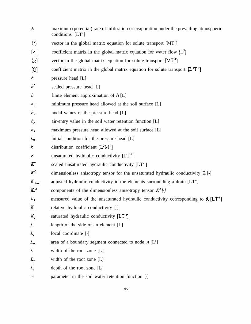
E

KlVI{g}[G]h

h'

h'

h A

h”h.7

hshllk

K

K’

KA

Kdram

KyA4KrKSL

4L”4

L.vLm

maximum (potential) rate of infiltration or evaporation under the prevailing atmosphericconditions [LT’]

vector in the global matrix equation for solute transport [MT’]

coefficient matrix in the global matrix equation for water flow [L3]

vector in the global matrix equation for solute transport [MT-‘]

coefficient matrix in the global matrix equation for solute transport [L3Te’]

pressure head [L]

scaled pressure head [L]

finite element approximation of h [L]

minimum pressure head allowed at the soil surface [L]

nodal values of the pressure head [L]

air-entry value in the soil water retention function [L]

maximum pressure head allowed at the soil surface [L]

initial condition for the pressure head [L]

distribution coefficient [L3M-‘1

unsaturated hydraulic conductivity [LT-‘1

scaled unsaturated hydraulic conductivity [LT“]

dimensionless anisotropy tensor for the unsaturated hydraulic conductivity K [-]

adjusted hydraulic conductivity in the elements surrounding a drain [LT“]

components of the dimensionless anisotropy tensor KA [-]

measured value of the unsaturated hydraulic conductivity corresponding to Ok [LT-‘1

relative hydraulic conductivity [-]

saturated hydraulic conductivity [LT-‘1

length of the side of an element [L]

local coordinate [-]

area of a boundary segment connected to node n [L’]

width of the root zone [L]

width of the root zone [L]

depth of the root zone [L]

parameter in the soil water retention function [-]

xvi

4i

Q,"

QR

Q,'

{Q>

[Ql

R

cumulative amount of solute removed from the flow region by zero-order reactions [M]

cumulative amount of solute removed from the flow region by first-order reactions [M]

cumulative amount of solute removed from the flow region by root water uptake [M]

amount of solute in the flow region at time t [M]

amount of solute in element e at time t [M]

amount of solute in the flow region at the beginning of the simulation [M]

amount of solute in element e at the beginning of the simulation [Mj

exponent in the soil water retention function [-]

components of the outward unit vector normal to boundary rN [-]

total number of nodes [-]

number of subelements e, which contain node n [-]

actual rate of inflow/outflow to/from a subregion [L3TS’]

local Peclet number [-]

components of the Darcian fluid flux density [LT“]

convective solute flux at node n [MT?]

dispersive solute flux at node n [MT’]

total solute flux at node n Frr_‘]

vector in the global matrix equation for water flow [L3T’]

coefficient matrix in the global matrix equation for solute transport [L3]

retardation factor [-]

adsorbed solute concentration [-]

sink term CT-‘]

degree of saturation [-]

degree of saturation corresponding to 0, [-I

spatial distribution of the potential transpiration rate [T“]

soil surface associated with transpiration [L2]

coefficient matrix in the global matrix equation for solute transport [L3Tm’]

time [T]

actual transpiration rate per unit surface length [LT“]

xvii

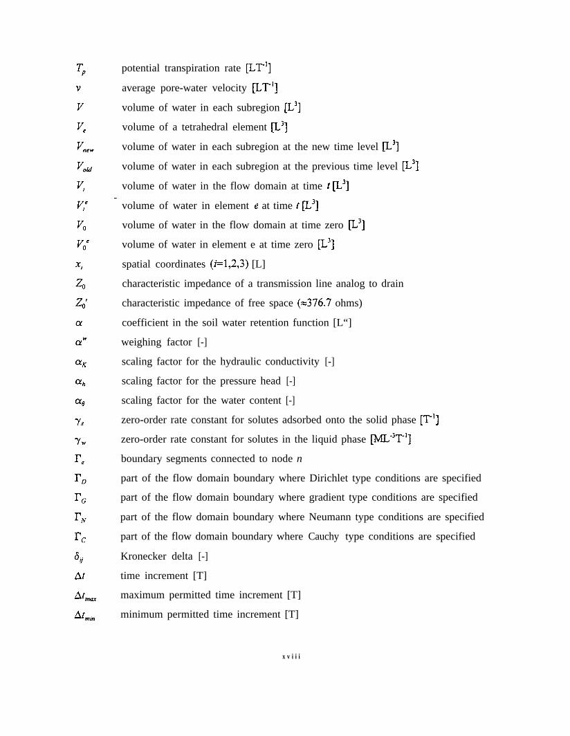
potential transpiration rate [LT-‘1

average pore-water velocity [LT-‘1

volume of water in each subregion [L3]

volume of a tetrahedral element [L3]

volume of water in each subregion at the new time level [L3]

volume of water in each subregion at the previous time level [L3]

volume of water in the flow domain at time t [L3]

volume of water in element e at time t [L3]

volume of water in the flow domain at time zero [L3]

volume of water in element e at time zero [L3]

spatial coordinates (i=l,2,3) [L]

characteristic impedance of a transmission line analog to drain

characteristic impedance of free space (~376.7 ohms)

coefficient in the soil water retention function [L“]

weighing factor [-]

scaling factor for the hydraulic conductivity [-]

scaling factor for the pressure head [-]

scaling factor for the water content [-]

zero-order rate constant for solutes adsorbed onto the solid phase [T’]

zero-order rate constant for solutes in the liquid phase [ML”T’]

boundary segments connected to node n

part of the flow domain boundary where Dirichlet type conditions are specified

part of the flow domain boundary where gradient type conditions are specified

part of the flow domain boundary where Neumann type conditions are specified

part of the flow domain boundary where Cauchy type conditions are specified

Kronecker delta [-]

time increment [T]

maximum permitted time increment [T]

minimum permitted time increment [T]

x v i i i

PFL,

PL,

PO

P

Pd

u

7

temporal weighing factor [-]

absolute error in the solute mass balance [M]

absolute error in the water mass balance (L3]

relative error in the solute mass balance [%]

relative error in the water mass balance [%]

permittivity of free space (used in electric analog representation of drains)

volumetric water content [L3L”]

scaled volumetric water content [L3L”]

parameter in the soil water retention function [L3LS3]

volumetric water content corresponding to Kk [L3Le3]

parameter in the soil water retention function [L3LS3]

residual soil water content [L3L”]

saturated soil water content [L3L03]

first-order rate constant [T’]

first-order rate constant for solute adsorbed onto the solid phase CT’]

first-order rate constant for solutes in the liquid phase [T’]

permeabihty of free space

bulk density [ML”]

dimensionless ratio between the side of the square in the finite element meshsurrounding the drain, D, and the effective diameter of a drain, d

prescribed flux boundary condition at boundary rN [LIT’]

tortuosity factor [-]

linear basis functions [-]

upstream weighted basis functions [-]

prescribed pressure head boundary condition at boundary I?0 [L]

performance index used as a criterion to minimize or eliminate numerical oscillations

[-]flow region

domain occupied by element e

region occupied by the root zone

xix

1. INTRODUCTION

The importance of the unsaturated zone as an integral part of the hydrological cycle has

long been recognized. The zone plays an inextricable role in many aspects of hydrology,

including infiltration, soil moisture storage, evaporation, plant water uptake, groundwater

recharge, runoff and erosion. Initial studies of the unsaturated (vadose) zone focused primarily

on water supply studies, inspired in part by attempts to optimally manage the root zone of

agricultural soils for maximum crop production. Interest in the unsaturated zone has dramatically

increased in recent years because of growing concern that the quality of the subsurface

environment is being adversely affected by agricultural, industrial and municipal activities.

Federal, state and local action and planning agencies, as well as the public at large, are now

scrutinizing the intentional or accidental release of surface-applied and soil-incorporated chemicals

into the environment. Fertilizers and pesticides applied to agricultural lands inevitably move

below the soil root zone and may contaminate underlying groundwater reservoirs. Chemicals

migrating from municipal and industrial disposal sites also represent environmental hazards. The

same is true for radionuclides emanating from energy waste disposal facilities.

The past several decades have seen considerable progress in the conceptual understanding

and mathematical description of water flow and solute transport processes in the unsaturated zone.

A variety of analytical and numerical models are now available to predict water and/or solute

transfer processes between the soil surface and the groundwater table. The most popular models

remain the Richards’ equation for variably saturated flow, and the Fickian-based convection-

dispersion equation for solute transport. Deterministic solutions of these classical equations have

been used, and likely will continue to be used in the near future, for predicting water and solute

movement in the vadose zone, and for analyzing specific laboratory or field experiments

involving unsaturated water flow and/or solute transport. These models are also helpful tools for

extrapolating information from a limited number of field experiments to different soil, crop and

climatic conditions, as well as to different tillage and water management schemes.

The purpose of this report is to document version 1.0 of the SWMS_3D computer

program simulating water and solute movement in three-dimensional variably saturated media.

The program numerically solves the Richards’ equation for saturated-unsaturated water flow and

1

the convection-dispersion equation for solute transport. The flow equation incorporates a sink

term to account for water uptake by plant roots. The solute transport equation includes provisions

for linear equilibrium adsorption, zero-order production, and first-order degradation. The

program may be used to analyze water and solute movement in unsaturated, partially saturated,

or fully saturated porous media. SWMS_3D can handle flow domains delineated by irregular

boundaries. The flow region itself may be composed of nonuniform soils having an arbitrary

degree of local anisotropy. The water flow part of the model considers prescribed head and flux

boundaries, as well as boundaries controlled by atmospheric conditions or free drainage. A

simplified representation of nodal drains using results of electric analog experiments is also

included. First- or third-type boundary conditions can be prescribed in the solute transport part

of the model.

The governing flow and transport equations are solved numerically using Galerkin-type

linear finite element schemes. Depending upon the size of the problem, the matrix equations

resulting from discretization of the governing equations are solved using either Gaussian

elimination for banded matrices, or the conjugate gradient method for symmetric matrices and

the ORTHOMIN method for asymmetric matrices [Mendoza et. al., 1991]. The program is an

extension of the variably saturated transport code SWMS_2D (version 1.2) of hnz.Znek et al.

[1994]. The SWMS_3D code is written in ANSI standard FORTRAN 77, and hence can be

compiled, linked and run on any standard micro-, mini-, or mainframe system, as well as on

personal computers. The source code was developed and tested on a P5 using the Microsoft

FORTRAN PowerStation.

This report serves as both a user manual and reference document. Detailed instructions

are given for data input preparation. Example input and selected output files are aiso provided.

3 % inch floppy diskette containing the source code and the selected input and output files of four

examples discussed in this report are available upon request from the authors.

2

2. VARIABLY SATURATED WATER FLOW

2.1. Governing Flow Equation

Consider three-dimensional isothermal Darcian flow of water in a variably saturated rigid

porous medium and assume that the air phase plays an insignificant role in the liquid flow

process. The governing flow equation for these conditions is given by the following modified

form of the Richards’ equation:

ae-=-ap(,,g +K31 -sat , J

(2-l)

where 8 is the volumetric water content [L3Lm3], h is the pressure head [L], S is a sink term [T’],

xi (i=1,2,3) are the spatial coordinates [L] , t is time [T], K,” are components of a dimensionless

tensor KA representing the possible anisotropic nature of the medium, and K is the unsaturated

hydraulic conductivity function [LT-‘1 given by

(2.2)

where K, is the relative hydraulic conductivity [-] and K, the principal saturated hydraulic

conductivity [LT-‘I. According to this definition, the value of K,” in (2.1) must be positive and

less than or equal to unity. The diagonal entries of K,” equal one and the off-diagonal entries

zero for an isotropic medium. Einstein’s summation convention is used in (2.1) and throughout

this report. Hence, when an index appears twice in an algebraic term, this particular term must

be summed over all possible values of the index.

2.2. Root Water Uptake

The sink term, S. in (2.1) represents the volume of water removed per unit time from a

unit volume of soil due to plant water uptake. Feddes et al. [ 1978] defined S as

S(h) = a(h)Sp (2.3)

where the water strkss response function a(h) is a prescribed dimensionless function (Fig. 2.1)

of the soil water pressure head (05u<l), and SP is the potential water uptake rate [T’]. Figure

2.1. gives a schematic plot of the stress response function as used by Feddes et al. [ 1978].

Notice that water uptake is assumed to be zero close to saturation (i.e., wetter than some arbitrary

“anaerobiosis point”, h,). For Hz, (the wilting point pressure head), water uptake is also

assumed to be zero. Water uptake is considered optimal between pressure heads h, and h,,

whereas for pressure head between h, and h, (or h, and h,), water uptake changes linearly with

h. The potential water uptake SP

stress, i.e., a(h)=l.

When the potential water

is equal to the water uptake rate during periods of no water

uptake rate is equally distributed over a three-dimensional

rectangular root domain, 5” becomes

I.21I

1.0

0.8

0.6

0.4

0.2

0

Pressure Head,h

Fig. 2.1. Schematic of the plant water stress response function, a(h),as used by Feddes et al. [ 1978].

Fig. 2.2. Schematic of the potential water uptake distribution function, b(x,ys),in the soil root zone.

S, = LS, T, (2.4)=x=y= f

where Tp is the potential transpiration rate [LT’], L, is the depth [L] of the root zone, L, and Lv

are the lateral widths [L] of the root zone, and S, is the area of the soil surface [L’] associated

with the transpiration process. Notice that SP reduces to TJL, when S,=L.&.

Equation (2.4) may be generalized by introducing a non-uniform distribution of the

potential water uptake rate over a root zone of arbitrary shape:

S, = b(x, y, 2) S, T, (2.5)

where b(x,y,t) is the normalized water uptake distribution [Ls3]. This function describes the

spatial variation of the potential extraction term, S,,, over the root zone (Fig. 2.2), and is obtained

from b’(~,y,z) as follows

b(x,y,z) = b ‘(xJsz)

d b '(X,Y,Z> dQ (2.6)

”

where 8, is the region occupied by the root zone, and b’(x,y,z) is an arbitrarily prescribed

distribution function. Normalizing the uptake distribution ensures that b(x,y,z) integrates to unity

over the flow domain, i.e.,

I b(x,y,z) dQ = 14

From (2.5) and (2.7) it follows that SP is related to Tp by the expression

’-s;

SpdQ= T,

(2.7)

(2.8)

The actual water uptake distribution is obtained by substituting (2.5) into (2.3):

WV,Y,~ = a(kx,y,z) KGYJ) S, T, (2.9)

whereas the actual transpiration rate, T,, is obtained by integrating (2.9) as follows

T, = $ 6”” = T, [a(h,x,y,z) b(x,y,z)dQ (2.10)

2.3. The Unsaturated Soil Hydraulic Properties

The unsaturated soil hydraulic properties in the SWMS_3D code are described by a set

of closed-form equations resembling those of van Genuchten [ 1980] who used the statistical pore-

size distribution model of Mualem [ 1976] to obtain a predictive equation for the unsaturated

hydraulic conductivity function. The original van Genuchten equations were modified to add

extra flexibility in the description of the hydraulic properties near saturation [sir et al., 1985;

Vogel and Cislerovb, 1988]. The soil water retention, B(h), and hydraulic conductivity, K(h),

functions in SWMS_3D are given by

L ea+ enl -e,8(h) = (1 + IQW)”

es

and

(h - h,)Ws - K,)h _ h

* k

respectively, where

K, = ;s

F(B) =

h<hs

hsh,

hk<h<hs

I e -ea

em - 0,

m=l-l/n , n>l

e -erse = -es - 87

s ‘k - ‘r

(2.11)

(2.12)

(2.13)

(2.14)

(2.15)

(2.16)

(2.17)

in which 8, and 8, denote the residual and saturated water contents, respectively, and K, is the

saturated hydraulic conductivity. To increase the flexibility of the analytical expressions, and to

allow for a non-zero air-entry value, h,, the parameters 8, and 0, in the retention function were

7

hsPressure Head, h

,e, =Qri0>

Fig. 2.3. Schematics of the soil water retention (a) and hydraulic conductivity (b) functionsas given by equations (2.11) and (2.12), respectively.

Linear interpolationKS

KkMualem’s model

”

hk hs ’

Pressure Head, h

replaced by the fictitious (extrapolated) parameters 0s8, and e&t?, as shown in Fig. 2.3. The

approach maintains the physical meaning of 8, and 0, as measurable quantities. Equation (2.13)

assumes that the predicted hydraulic conductivity function is matched to a measured value of the

hydraulic conductivity, K,=K(eJ, at some water content, 8, less that or equal to the saturated

water content, i.e., (368, and K$.K$ [Vogel and Cislerovci, 1988; Luckner et al., 1989].

Inspection of (2.11) through (2.17) shows that the hydraulic characteristics contain 9

unknown parameters: e,, e,, e,, e,, a, n, K,, Kk, and ek. When 8,,=0,, e,=e,=e, and K,=K,

the soil hydraulic functions reduce to the original expressions of van Genuchten [ 1980]:

0s -or h<O (2.18)8(h) =

I

er+ [l + ICY/r].],

0s h20

8

Kjqh> h<OK(h) =

K* h20

where

K, = &‘“[l - (1 - $“)“]*

(2.19)

(2.20)

2.4. Scaling of the Soil Hydraulic Functions

SWMS_3D implements a scaling procedure designed to simplify the description of the

spatial variability of the unsaturated soil hydraulic properties in the flow domain. The code

assumes that the hydraulic variability in a given area can be approximated by means of a set of

linear scaling transformations which relate the individual soil hydraulic characteristics 6(h) and

K(h) to reference characteristics B’(h’) and K’(h’). The technique is based on the similar media

concept introduced by Miller and Miller [1956] for porous media which differ only in the scale

of their internal geometry. The concept was extended by Simmons et al. [ 1979] to materials

which differ in morphological properties, but which exhibit ‘scale-similar’ soil hydraulic

functions. Three independent scaling factors are embodied in SWMS_3D. These three scaling

parameters may be used to define a linear model of the actual spatial variability in the soil

hydraulic properties as follows [Vogel et al., 1991]:

K(h) = cxxK*(h ‘)

8(h) =er+or,[OTh**)) -19~7 (2.21)

h =q,h l

in which, for the most general case, CX~, cz, and CQ are mutually independent scaling factors for

the water content, the pressure head and the hydraulic conductivity, respectively. Less general

scaling methods arise by invoking certain relationships between LY@, cy,, and/or Q. For example,

the original Miller-Miller scaling procedure is obtained by assuming ar,=l (with 8,* = O,), and

9

a,=cY,‘2. A detailed discussion of the scaling relationships given by (2.21), and their application

to the hydraulic description of heterogeneous soil profiles, is given by Vogel et al. [ 1991].

2.5. Initial and Boundary Conditions

The solution of Eq. (2.1) requires knowledge of the initial distribution of the pressure head

within the flow domain, Q:

W,YJ, 0 = h,(X,YA for t=O (2.22)

where h, is a prescribed function of x, y and z.

SWMS_3D implements three types of conditions to describe system-independent

interactions along the boundaries of the flow region. These conditions are specified pressure head

(Dirichlet type) boundary conditions of the form

@,y,z, t) = 4 (X,YA t> for (X,Y,Z> E ro (2.23)

specified flux (Neumann type) boundary conditions given by

-[K(KpJ + K,A)] ni = ~,(x,y,z, 4

and specified gradient boundary conditions

“.k.J

(K;g + &f)n; = a,(x,y,z, t)J

(2.24)

where I’D, TN, and rc indicate Dirichlet, Neumann, and gradient type boundary segments,

respectively; $ [L], (I~ [LT-‘1, and 0, [-] are prescribed functions of x, y, z and t; and nj are the

components of the outward unit vector normal to boundary rN or rc. As pointed out by McCord

[ 199 1], the use of the term “Neumann type boundary condition” for the flux boundary is not very

appropriate since this term should hold for a gradient type condition (see also Section 3.2 for

solute transport). However, since the use of the Neumann condition is standard in the hydrologic

literature [Neuman, 1972; Neuman et al., 1974], we shall also use this term to indicate flux

10

boundaries throughout this report. SWMS_3D implements the gradient boundary condition only

in terms of a unit vertical hydraulic gradient (a2 = 1) simulating free drainage from a relatively

deep soil profile. This situation is often observed in field studies of water flow and drainage in

the vadose zone [Sisson, 1987; McCord, 1991]. McCord [ 1991] states that the most pertinent

application of (2.25) is its use as a bottom outflow boundary condition for situations where the

water table is situated far below the domain of interest.

In addition to the system-independent boundary conditions given by (2.23), (2.24), and

(2.25), SWMS_3D considers three different types of system-dependent boundary conditions which

cannot be defined a priori. One of these involves soil-air interfaces which are exposed to

atmospheric conditions. The potential fluid flux across these interfaces is controlled exclusively

by external conditions. However, the actual flux depends also on the prevailing (transient) soil

moisture conditions. Soil surface boundary conditions may change from prescribed flux to

prescribed head type conditions (and vice-versa). In the absence of surface ponding, the

numerical solution of (2.1) is obtained by limiting the absolute value of the flux such that the

following two conditions are satisfied [Neuman et al., 1974]:

+ KkA)nil I EJ

and

h, I h I h,

(2.26)

(2.27)

where E is the maximum potential rate of infiltration or evaporation under the current

atmospheric conditions, h is the pressure head at the soil surface, and h,., and h, are, respectively,

minimum and maximum pressure heads allowed under the prevailing soil conditions. The value

for h, is determined from the equilibrium conditions between soil water and atmospheric water

vapor, whereas h, is usually set equal to zero. SWMS_3D assumes that any excess water on the

soil surface is immediately removed. When one of the end points of (2.27) is reached, a

prescribed head boundary condition will be used to calculate the actual surface flux. Methods

of calculating E and hA on the basis of atmospheric data have been discussed by Feddes et al.

[1974].

11

A second type of system-dependent boundary condition considered in SWMS_3D is a

seepage face through which water leaves the saturated part of the flow domain. In this case, the

length of the seepage face is not known a priori. SWMS_3D assumes that the pressure head is

always uniformly equal to zero along a seepage face. Additionally, the code assumes that water

leaving the saturated zone across a seepage face is immediately removed by overland flow or

some other removal process.

Finally, a third class of system-dependent boundary conditions in SWMS_3D concerns

tile drains. Similarly as for seepage phase, SWMS_3D assumes that as long as a drain is located

in the saturated zone, the pressure head along the drain will be equal to zero; the drain then acts

as a pressure head sink. However, the drain will behave as a nodal sink/source with zero

recharge when located in the unsaturated zone. More information can be found in Section 4.3.7.

12

3. SOLUTE TRANSPORT

3.1. Governing Transport Equation

The partial differential equation governing three-dimensional chemical transport during

transient water flow in a variably saturated rigid porous medium is taken as

ah + aps aq,c-=&j&ydt at , +lLwec +k$L,ps +yj fY,P --q (3.1)I I

where c is the solution concentration [ML^-3], s is the adsorbed concentration [-], qi is the i-th

component of the volumetric flux [LT’], CL, and pL, are first-order rate constants for solutes in the

liquid and solid phases [‘I?‘], respectively; y,,, and ys are zero-order rate constants for the liquid

[ML‘3T-1] and solid [T’] phases, respectively; p is the soil bulk density [ML^-3], S is the sink term

in the water flow equation (2.1), c, is the concentration of the sink term [MLs3], and D, is the

dispersion coefficient tensor [L*T’]. The four zero- and first-order rate constants in (3.1) may

be used to represent a variety of reactions or transformations including biodegradation,

volatilization, precipitation and radioactive decay.

SWMS_3D assumes equilibrium interactions between the solution (c) and adsorbed (s)

concentrations of the solute in the soil system. The adsorption isotherm relating s and c is further

assumed to be described by a linear equation of the form

s = kc

where k is an empirical constant [L3M-‘1.

The continuity equation for water flow

is given by

in a three-dimensional variably-saturated medium

de-=at

34;-q

- S (3.3)

(3.2)

where qi is the Darcian fluid flux density. Substituting (3.2) and (3.3) into (3.1) gives

13

where

F =/A,) +Cc,pk+S

G=ywe +y,p-SC3

and where the retardation factor R [-] is defined as

R=l+$

(3.4)

(3.5)

(3.6)

In order to solve equation (3.4), it is necessary to know the water content 8 and the

volumetric flux qP Both variables are obtained from solutions of the flow equation (2.1).

3.2. Initial and Boundary Conditions

The solution of (3.4) requires knowledge of the initial concentration within the flow

region, 112, i.e.,

’ (x,Y, ‘7 O ) = ci(x,Y,z) (3.7)

where ci is a prescribed function of x, y and z.

Two types of boundary conditions (Dirichlet and Cauchy type conditions) can be specified

along the boundary of 0. First-type (or Dirichlet type) boundary conditions prescribe the

concentration along a boundary segment r,:

C(&Y,4f) = c,(x,YJ,t) for kY,.e E Q (3.8)

whereas third-type (Cauchy type) boundary conditions may be used to prescribe the solute flux

along a boundary segment I?e as follows:

14

-6D..dcn.+q.n.c=q.n,co fir (x,y,z)&rc“axi’ ” ’

in which qini represents the outward fluid flux, ni is the outward unit normal vector, and c, is the

concentration of the incoming fluid. In some cases, for example when rC is an impermeable

boundary (qi n,=O) or water flow is directed out of the region (qi n,c,=q, n,c), (3.9) reduces to a

second-type (Neumann type) boundary condition of the form:

fir (X9Y9.4 ‘2 q/

3.3. Dispersion Coefficient

The components of the dispersion tensor, D,, in (3.1) are given by [Bear, 1972]

(3.10)

(3.11)

where D, is the ionic or molecular diffusion coefficient in free water [L2T0’], r is a tortuosity

factor [-], 1 q 1 is the absolute value of the Darcian fluid flux density [LTl], 6, is the Kronecker

delta function (&=I if i=j, and S,=O if i#j), and DL and D, are the longitudinal and transverse

dispersivities, respectively [L]. The individual components of the dispersion tensor for three-

dimensional transport are as follows:

BD_,o,4:+D 4’2+D q,2I41 T 141 T 141

+8D,r

So_-0,4:+D 4,2+D141

T141

T q,2141

+OD,7

15

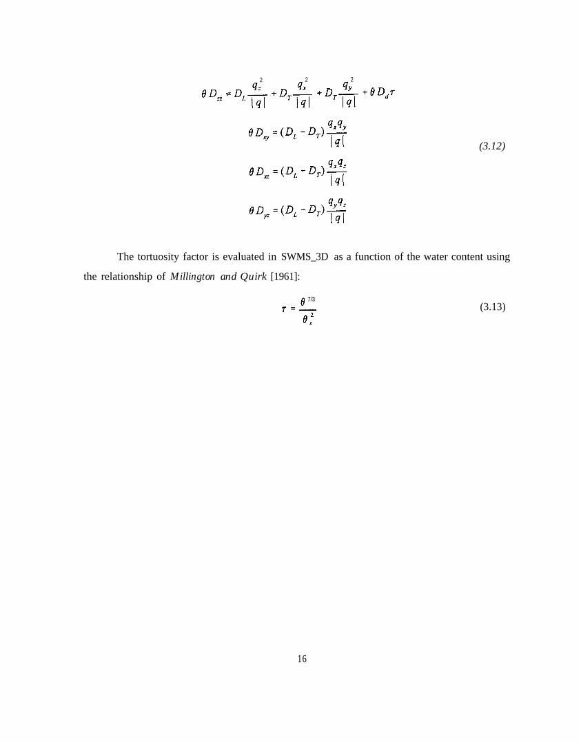
2 2 2

%D_ =D+ +D,-$ +D+$ +ODdr

Oo,=(D,-0,)s141

dDx=(DL-DT)=191

(3.12)

SD,==(D,-D,)g

The tortuosity factor is evaluated in SWMS_3D as a function of the water content using

the relationship of Millington and Quirk [1961]:

8 7/3

7=-

0,’

(3.13)

16

4. NUMERICAL SOLUTION OF THE WATER FLOW EQUATION

The Galerkin finite element method with linear basis functions is used to obtain a solution

of the flow equation (2.1) subject to the imposed initial and boundary conditions. Since the

Galerkin method is relatively standard and has been covered in detail elsewhere [Neuman, 1975;

Zienkiewicz, 1977; Pinder and Gray, 1977], only the most pertinent steps in the solution process

are given here.

4.1. Space Discretization

The flow region is divided into a network of tetrahedral elements. The corners of these

elements are taken to be the nodal points. The dependent variable, the pressure head function

h(x,y,z,t), is approximated by a function h’(x,y,z,t) as follows

(4.1)

where 4, are piecewise linear basis functions satisfying the condition $&~,,y,,,,z,)=&,,, h, are

unknown coefficients representing the solution of (2.1) at the nodal points, and N is the total

number of nodal points.

The Galerkin method postulates that the differential operator associated with the Richards’

equation (2.1) is orthogonal to each of the N basis functions, i.e.,

Applying Green’s first identity to (4.2), and replacing h by h’, leads to

(4.2)

17

J ’

(4.3)

=IK(K,“dh + KizA)n;qQir + c %I( -KKcA-- - S4,,MQe ax, e ax,

c r

where Q2, represents the domain occupied by element e, and I’, is a boundary segment coinciding

with element e. Natural flux-type (Neumann) and gradient type boundary conditions can be

immediately incorporated into the numerical scheme by specifying the surface integral in equation

(4.3).

After imposing additional simplifying assumptions to be discussed later, and performing

integration over the elements, the procedure leads to a system of time-dependent ordinary

differential equations with nonlinear coefficients. In matrix form, these equations are given by

where

q ad,-"dQaxi axj

= c .&- [K,A b,,b, + K;cmcne 36VC

+ K,Adndm + K,A( bn,cn + cmbn) +

+ K,” ( b$n, + d, b,,,)

(4.4)

(4.5)

(4.6)

18

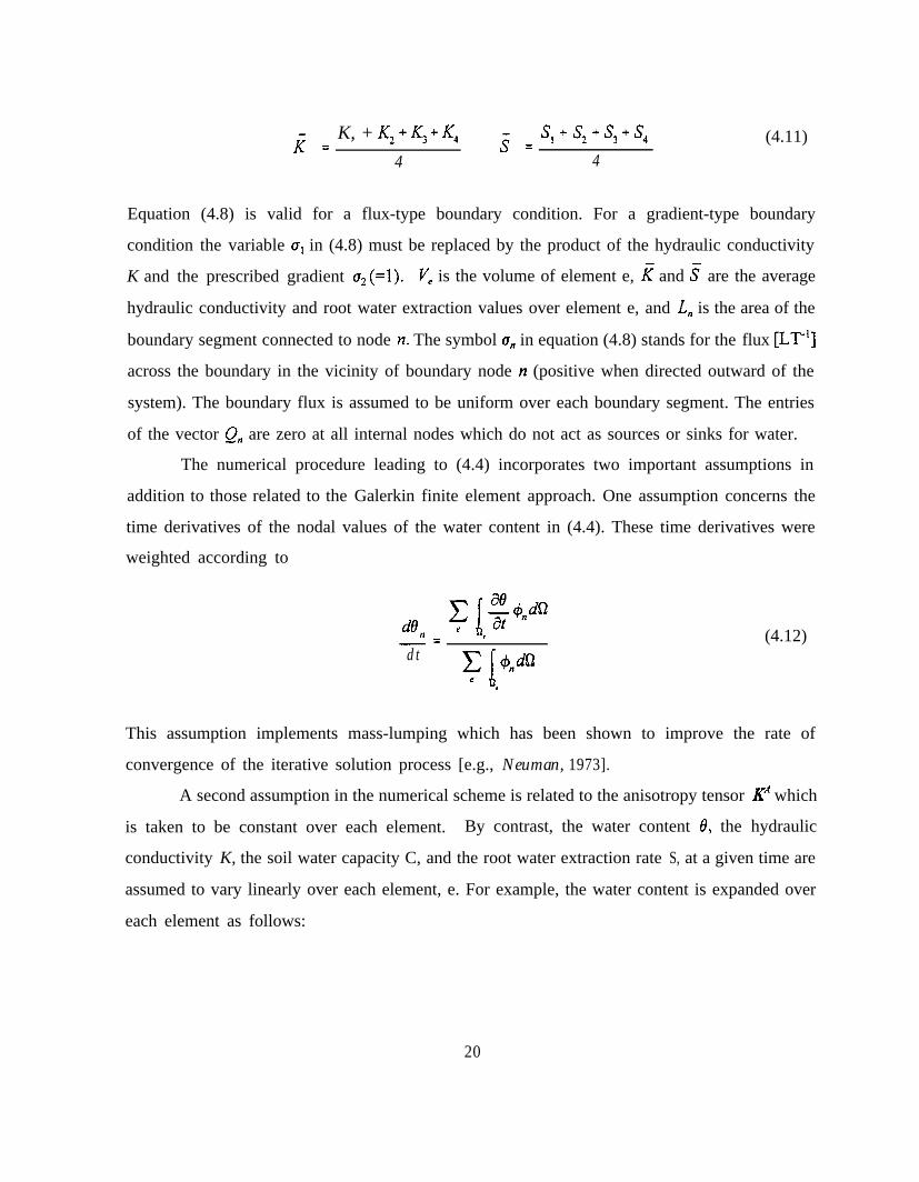
2 = K, + K2 + K3 + K4 j = s, + sz + s3 + s4

4 4(4.11)

Equation (4.8) is valid for a flux-type boundary condition. For a gradient-type boundary

condition the variable 0, in (4.8) must be replaced by the product of the hydraulic conductivity

K and the prescribed gradient aZ (=l). V, is the volume of element e, I? and ? are the average

hydraulic conductivity and root water extraction values over element e, and L, is the area of the

boundary segment connected to node n. The symbol a, in equation (4.8) stands for the flux [LT-‘1

across the boundary in the vicinity of boundary node n (positive when directed outward of the

system). The boundary flux is assumed to be uniform over each boundary segment. The entries

of the vector Q, are zero at all internal nodes which do not act as sources or sinks for water.

The numerical procedure leading to (4.4) incorporates two important assumptions in

addition to those related to the Galerkin finite element approach. One assumption concerns the

time derivatives of the nodal values of the water content in (4.4). These time derivatives were

weighted according to

-= (4.12)dt cd $,dQ

c,

This assumption implements mass-lumping which has been shown to improve the rate of

convergence of the iterative solution process [e.g., Neuman, 1973].

A second assumption in the numerical scheme is related to the anisotropy tensor KA which

is taken to be constant over each element. By contrast, the water content 0, the hydraulic

conductivity K, the soil water capacity C, and the root water extraction rate S, at a given time are

assumed to vary linearly over each element, e. For example, the water content is expanded over

each element as follows:

20

6) kYY4 = f: 0 (x,,Y",zn)~n(x,Y,4 for (X,Y,Z) E ye (4.13)n-1

where n stands for the comers of element e. The advantage of linear interpolation is that no

numerical integration is needed to evaluate the coefficients in (4.4).

4.2. Time Discretization

Integration of (4.4) in time is achieved by discretizing the time domain into a sequence

of finite intervals and replacing the time derivatives by finite differences. An implicit (backward)

finite difference scheme is used for both saturated and unsaturated conditions:

(4.14)

wherei+ 1 denotes the current time level at which the solution is being considered, i refers to the

previous time level, and A$=?,,& Equation (4.14) represents the final set of algebraic equations

to be solved. Since 8 and the coefficients A, B, D, and Q (for a gradient-type boundary

conditions) are functions of the dependent variable h, the set of equations is generally highly

nonlinear. Note that vectors D and Q, in contrast to the fully implicit scheme, are evaluated at

the old time level. This feature may, in some cases, improve the convergence rate.

4.3. Numerical Solution Strategies

4.3.1. Iteration Process

Because of the nonlinear nature of (4.14), an iterative process must be used to obtain

solutions of the global matrix equation at each new time step. For each iteration a system of

linearized algebraic equations is first derived from (4.14) which, after incorporation of the

boundary conditions, is solved using either Gaussian elimination or the conjugate gradient method

(see Section 6.5). The Gaussian elimination process takes advantage of the banded and

21

symmetric features of the coefficient matrices in (4.14). After inversion, the coefficients in (4.14)

are re-evaluated using the first solution, and the new equations are again solved. The iterative

process continues until a satisfactory degree of convergence is obtained, i.e., until at all nodes in

the saturated (or unsaturated) region the absolute change in pressure head (or water content)

between two successive iterations becomes less than the imposed absolute pressure head (or water

content) tolerance [&mJnek and Suarez, 1993]. The first estimate (at zero iteration) of the

unknown pressure heads at each time step is obtained by extrapolation from the pressure head

values at the previous two time levels.

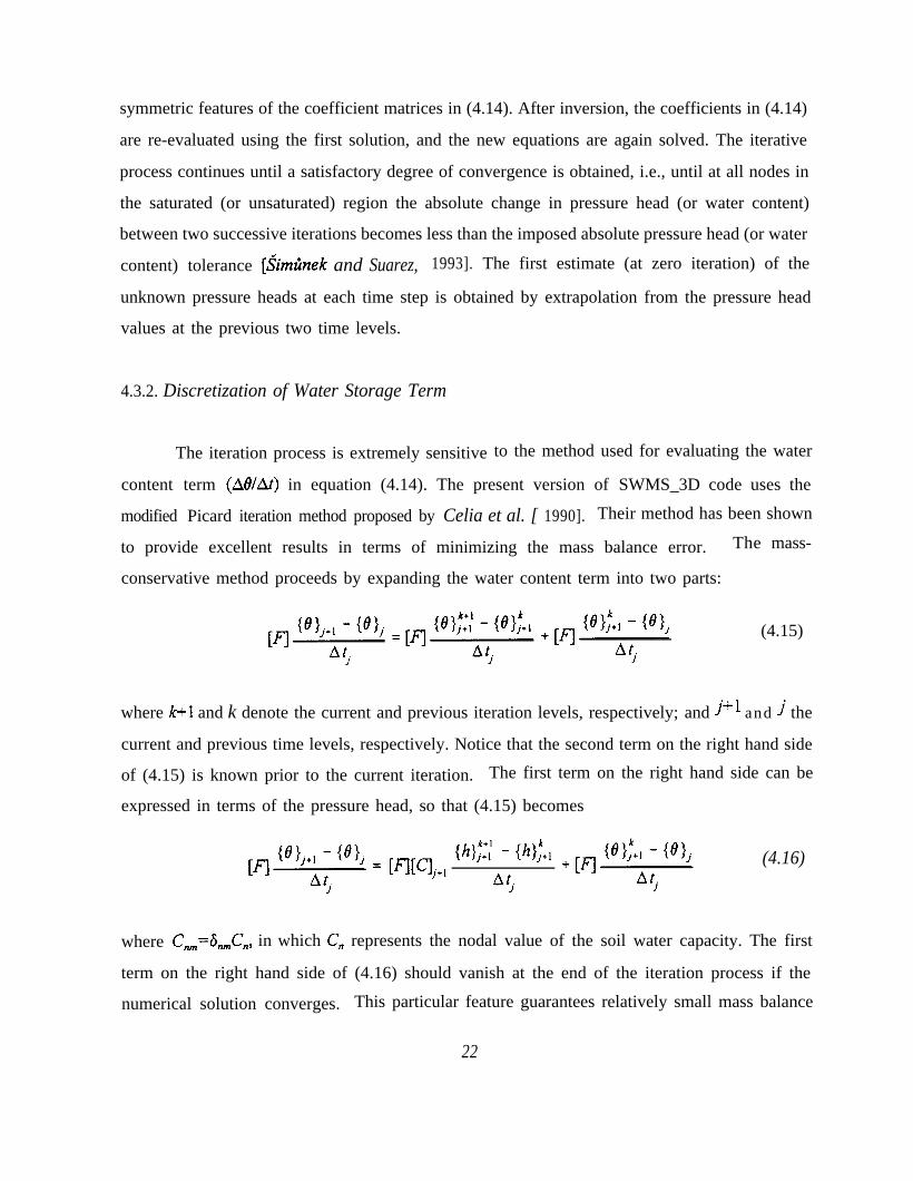
4.3.2. Discretization of Water Storage Term

The iteration process is extremely sensitive to the method used for evaluating the water

content term (AelAt) in equation (4.14). The present version of SWMS_3D code uses the

modified Picard iteration method proposed by Celia et al. [ 1990]. Their method has been shown

to provide excellent results in terms of minimizing the mass balance error. The mass-

conservative method proceeds by expanding the water content term into two parts:

(4.15)

where k+l and k denote the current and previous iteration levels, respectively; and j+l and j the

current and previous time levels, respectively. Notice that the second term on the right hand side

of (4.15) is known prior to the current iteration. The first term on the right hand side can be

expressed in terms of the pressure head, so that (4.15) becomes

= iI4 [cl,+,

w;:: - (h);+, (4.16)Afj

where C,,,,--&,,,C,, in which C, represents the nodal value of the soil water capacity. The first

term on the right hand side of (4.16) should vanish at the end of the iteration process if the

numerical solution converges. This particular feature guarantees relatively small mass balance

22

errors in the solution.

4.3.3. Time Step Control

Three different time discretizations are introduced in SWMS_3D: (1) time discretizations

associated with the numerical solution, (2) time discretizations associated with the implementation

of boundary conditions, and (3) time discretizations which provide printed output of the

simulation results (e.g., nodal values of dependent variables, water and solute mass balance

components, and other information about the flow regime).

Discretizations 2 and 3 are mutually independent; they generally involve variable time

steps as described in the input data file. Discretization 1 starts with a prescribed initial time

increment, At. This time increment is automatically adjusted at each time level according to the

following rules [Mls, 1982; Vogel, 1987]:

a. Discretization 1 must coincide with time values resulting from discretizations 2 and

3.

b. Time increments cannot become less than a preselected minimum time step, A&, nor

exceed a maximum time step, At_ (i.e., At,, < At I At_).

c. If, during a particular time step, the number of iterations necessary to reach

convergence is 13, the time increment for the next time step is increased by

multiplying At by a predetermined constant >l (usually between 1.1 and 1.5). If the

number of iterations is 27, At for the next time level is multiplied by a constant <1

(usually between 0.3 and 0.9).

d. If, during a particular time step, the number of iterations at any time level becomes

greater than a prescribed maximum (usually between 10 and 50), the iterative process

for that time level is terminated. The time step is subsequently reset to &/3, and the

iterative process restarted.

The selection of optimal time steps, At, is also influenced by the solution scheme for solute

transport (see Section 5.3.6.).

23

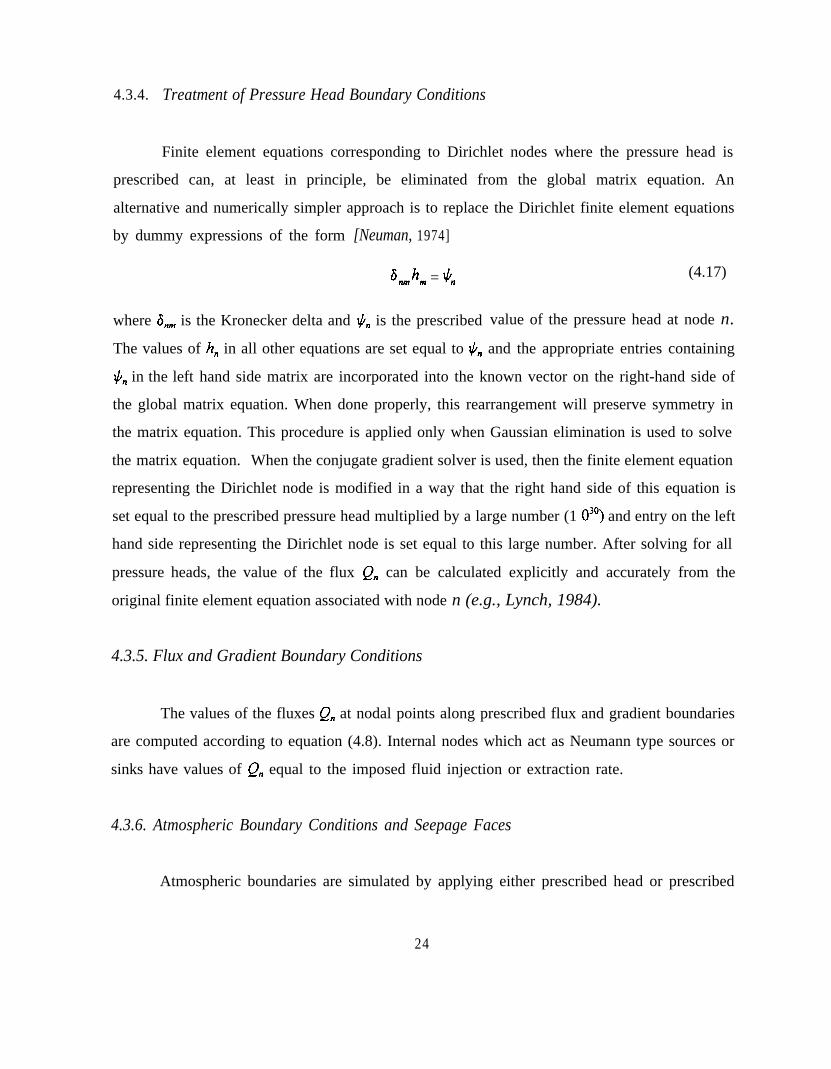
4.3.4. Treatment of Pressure Head Boundary Conditions

Finite element equations corresponding to Dirichlet nodes where the pressure head is

prescribed can, at least in principle, be eliminated from the global matrix equation. An

alternative and numerically simpler approach is to replace the Dirichlet finite element equations

by dummy expressions of the form [Neuman, 1974]

&Jr,,, = 1L, (4.17)

where d, is the Kronecker delta and 1c;, is the prescribed value of the pressure head at node n.

The values of h, in all other equations are set equal to $” and the appropriate entries containing

II/, in the left hand side matrix are incorporated into the known vector on the right-hand side of

the global matrix equation. When done properly, this rearrangement will preserve symmetry in

the matrix equation. This procedure is applied only when Gaussian elimination is used to solve

the matrix equation. When the conjugate gradient solver is used, then the finite element equation

representing the Dirichlet node is modified in a way that the right hand side of this equation is

set equal to the prescribed pressure head multiplied by a large number (1 03’) and entry on the left

hand side representing the Dirichlet node is set equal to this large number. After solving for all

pressure heads, the value of the flux Q, can be calculated explicitly and accurately from the

original finite element equation associated with node n (e.g., Lynch, 1984).

4.3.5. Flux and Gradient Boundary Conditions

The values of the fluxes Q, at nodal points along prescribed flux and gradient boundaries

are computed according to equation (4.8). Internal nodes which act as Neumann type sources or

sinks have values of Q” equal to the imposed fluid injection or extraction rate.

4.3.6. Atmospheric Boundary Conditions and Seepage Faces

Atmospheric boundaries are simulated by applying either prescribed head or prescribed

24

flux boundary conditions depending upon whether equation (2.26) or (2.27) is satisfied [Neuman,

1974]. If (2.27) is not satisfied, node n becomes a prescribed head boundary, If, at any point

in time during the computations, the calculated flux exceeds the specified potential flux in (2.26),

the node will be assigned a flux equal to the potential value and treated again as a prescribed flux

boundary.

All nodes expected to be part of a seepage face during code execution must be identified

a priori. During each iteration, the saturated part of a potential seepage face is treated as a

prescribed pressure head boundary with h=O, while the unsaturated part is treated as a prescribed

flux boundary with Q=O. The lengths of the two surface segments are continually adjusted

[Neuman, 1974] during the iterative process until the calculated values of Q (equation (4.8))

along the saturated part, and the calculated values of h along the unsaturated part, are all negative,

thus indicating that water is leaving the flow region through the saturated part of the surface

boundary only.

4.3.7. Treatment of Tile Drains

The representation of tile drains as boundary conditions is based on studies by Vimoke et

al. [ 1963] and Fipps et al. [1986]. The approach uses results of electric analog experiments

conducted by Vimoke and Taylor [ 1962] who reasoned that drains can be represented by nodal

points in a regular finite element mesh, provided adjustments are made in the hydraulic

conductivity, K, of neighboring elements. The adjustments should correspond to changes in the

electric resistance of conducting paper as follows

Kdram = K 'd (4.18)

where K&jn is the adjusted conductivity [LT“], and Cd is the correction factor [-]. C, is

determined from the ratio of the effective radius, d [L], of the drain to the side length, D [L], of

the square formed by finite elements surrounding the drain node and located in a plane

perpendicular to a drain [ Vimoke at al., 1962]:

25

Cd =zd dPO’EO-xZ0 138 log,opd + 6.48 -2.34A - 0.48B - 0.12C

(4.19)

where 2,’ is the characteristic impedance of free space (~376.7 ohms), p, is the permeability of

free space, e. is the permittivity of free space, and 2, is the characteristic impedance of a

transmission line analog of the drain. The coefficients in (4.19) are given by

D 1 + 0.405 pj4pd

=- A =d 1 - o.405pi4

(4.20)

B =1 + O.l63p,*

1 - O.l63p,*c =

1 + 0.067~;‘~

1 - 0.067~;‘~

where the effective drain diameter, d, is to be calculated from the number and size of small

openings in the drain tube [Mohammad and Skaggs, 1984], and D is the size of the square in the

finite element mesh surrounding the drain having adjusted hydraulic conductivities. The approach

above assumes that the node representing a drain must be surrounded by finite elements (either

triangular or quadrilateral) which form a square whose hydraulic conductivities are adjusted

according to (4.18). This method of implementing the drain by means of a boundary condition

gives an efficient, yet relatively accurate, prediction of the hydraulic head in the immediate area

surrounding the dram, as well as of the dram flow rates [Fipps et al., 1986]. More recent studies

have shown that the correction factor C, could be further reduced by a factor of 2 [Rogers and

Fouss, 1989] or 4 [Tseng, 1994, personal communication].

4.3.8. Water Balance Evaluation

The SWMS_3D code performs water balance computations at prescribed times for several

preselected subregions of the flow domain. The water balance information for each subregion

consists of the actual volume of water, V, in that subregion, and the rate, 0, of inflow or outflow

to or from the subregion. Y and 0 are given by

26

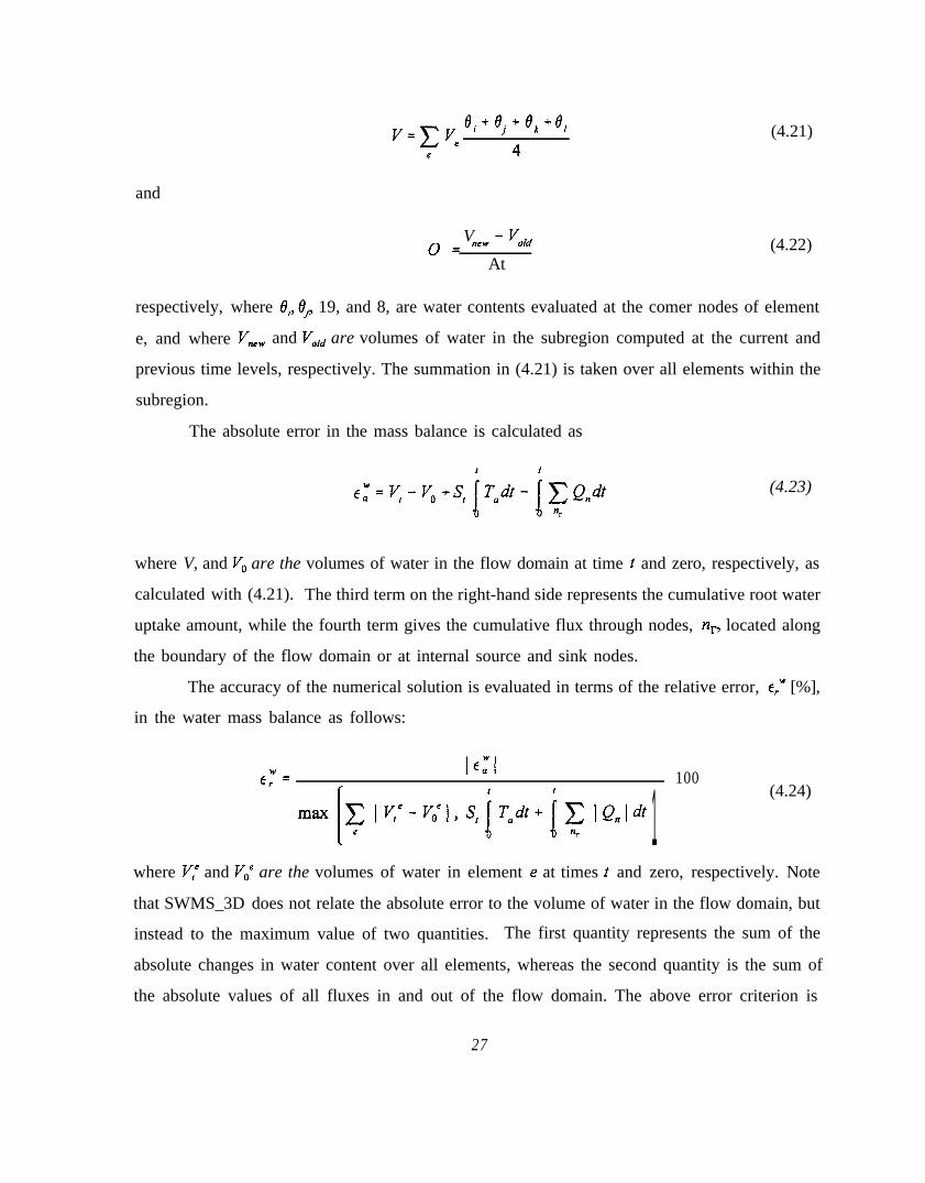
ej + ej + 8, + 0,v=Cr 4

c

(4.21)

and

V0 = *ew - V&i (4.22)At

respectively, where 0, O,, 19, and 8, are water contents evaluated at the comer nodes of element

e, and where V,,, and Vo,d are volumes of water in the subregion computed at the current and

previous time levels, respectively. The summation in (4.21) is taken over all elements within the

subregion.

The absolute error in the mass balance is calculated as

t

c Q,dt (4.23)

“r

where V, and V. are the volumes of water in the flow domain at time t and zero, respectively, as

calculated with (4.21). The third term on the right-hand side represents the cumulative root water

uptake amount, while the fourth term gives the cumulative flux through nodes, n,, located along

the boundary of the flow domain or at internal source and sink nodes.

The accuracy of the numerical solution is evaluated in terms of the relative error, E,~ [%],

in the water mass balance as follows:

E: = Kl 100

1(4.24)

where V,e and Voe are the volumes of water in element e at times t and zero, respectively. Note

that SWMS_3D does not relate the absolute error to the volume of water in the flow domain, but

instead to the maximum value of two quantities. The first quantity represents the sum of the

absolute changes in water content over all elements, whereas the second quantity is the sum of

the absolute values of all fluxes in and out of the flow domain. The above error criterion is

27

much stricter than the usual criterion involving the total volume of water in the flow domain.

This is because the cumulative boundary fluxes are often much smaller than the volume in the

domain, especially at the beginning of the simulation.

4.3.9. Computation of Nodal Fluxes

Components of the Darcian flux are computed at each time level during the simulation

only when the water flow and solute transport equations are solved simultaneously. When the

flow equation is being solved alone, the flux components are calculated only at selected print

times. The X-, y-, and z-components of the nodal fluxes are computed for each node n according

to:

K”4,=-NC[

y’h, + y,%, + y;hk + yfh,+K,Al

e e” 6 v,

4,=-f+y;hi + y;h, + y;hk + yj”h,

+ K;lI? 4 6 v,

Kn41=-$[

y,:hi + y,:hj + y;h, + y;h,+ K,A]

e e” 6 v,

(4.25)

y;=K,Ab,,+K&,+K;d,,

y; = K;b,, + K;c,, + K;d,

y;=K,Ab,,+KyAc,,+K,Adn

where N, is the number of sub-elements e, adjacent to node n. Einstein’s summation convention

is not used in (4.25).

4.3.10. Water Uptake by Plant Roots

SWMS_3D considers the root zone to consist of all nodes, n, for which the potential root

28

water uptake distribution, b (see Section 2.2), is greater than zero. The root water extraction rate

is assumed to vary linearly over each element; this leads to approximation (4.9) for the root water

extraction term D, in the global matrix equation. The values of actual root extraction rate S, in

(4.9) are evaluated with (2.9). In order to speed up the calculations, the extraction rates S,, are

calculated at the old time level and are not updated during the iterative solution process at a given

time step. SWMS_3D calculates the total rate of transpiration per unit soil surface length using

the equation

a=$ VjI e

(4.26)

in which the summation takes place over all elements within the root zone.

4.3.11. Evaluation of the Soil Hydraulic Properties

At the beginning of a numerical simulation, SWMS_3D generates for each soil type in

the flow domain a table of water contents, hydraulic conductivities, and specific water capacities

from the specified set of hydraulic parameters.

evaluated at prescribed pressure heads hi within a

table are generated such that

The values of 0, Ki and C; in the table are

specified interval (ha, hb). The entries in the

hi*,T

= constant (4.27)

which means that the spacing between two consecutive pressure head values increases in a

logarithmic fashion. Values for the hydraulic properties, 8(h), K(h) and C(h), are computed

during the iterative solution process using linear interpolation between the entries in the table.

If an argument h falls outside the prescribed interval (ha, hb), the hydraulic characteristics are

evaluated directly from the hydraulic functions, i.e., without interpolation. The above

interpolation technique was found to be much faster computationally than direct evaluation of the

hydraulic functions over the entire range of pressure heads, except when very simple hydraulic

29

models were used.

4.3.12. Implementation of Hydraulic Conductivity Anisotropy

Since the hydraulic conductivity anisotropy tensor, A?, is assumed to be symmetric, it is

possible to define at any point in the flow domain a local coordinate system for which the tensor

KA is diagonal (i.e., having zeroes everywhere except on the diagonal). The diagonal entries KIA,

KzA and KJA of KA are referred to as the principal components of K”.

The SWMS_3D code permits one to vary the orientation of the local principal directions

from element to element. For this purpose, the local coordinate axes are subjected to a rotation

such that they coincide with the principal directions of the tensor KA. The principal components

KIA, K2” and K3”, together with the cosines of angles between the principal directions of the tensor

K” and the axis of the global coordinate system, are specified for each element. Locally

determined principal components KIA, KzA and K3A are transformed to the global (x,y,z) coordinate

system at the beginning of the simulation using the following rules:

K,” = KIA a, I a, I + KzA aI2 aI2 + KJA aI3 aI3

Kd = 4” aI2 a,2 + K?” az2 al2 + GA az3 az3

K_:’ = K,‘4 aI3 al3 + KzA az3 az3 + K,” aJ3 aJ3

K,” = K,A a,, a,2 + KzA aI2 az2 + KJA a,3 az3

K,” = K,” a11 a13 + KIA al, az3 + KJA a,? aJ3.

&d = 4” aI2 q3 + GA a,, aT3 + GA az3 aJ3_ _

(4.28)

where a, represents cosine of angle between the ith principal direction of the tensor K” and the

j-axis of the global coordinate system.

30

4.3.13. Steady-State Analysis

All transient flow problems are solved by time marching until a prescribed time is

reached. The steady-state problem can be solved in the same way, i.e., by time marching until

two successive solutions differ less than some prescribed pressure head tolerance. SWMS_3D

implements a faster way of obtaining the steady-state solution without having to go through a

large number of time steps. The steady-state solution for a set of imposed boundary conditions

is obtained directly during one set of iterations at the first time step by equating the time

derivative term in the Richards’ equation (2.1) to zero.

31

5. NUMERICAL SOLUTION OF THE SOLUTE TRANSPORT EQUATION

The Galerkin finite element method is also used to solve solute transport equation (3.4)

subject to appropriate initial and boundary conditions. The solution procedure below largely

parallels the approach used for the flow equation.

5.1. Space Discretization

The dependent variable, the concentration function c(x,~,z,t), is approximated by a finite

series c’(xJJ,~) of the form

c’(x,y,z,O = 5 4”,(X,Y,Z> c,(t) (5.1)?I=1

where 4, are the selected linear basis functions, c, are the unknown time dependent coefficients

which represent solutions of (3.4) at the finite element nodal points and, as before, N is the total

number of nodal points. Application of the standard Galerkin method leads to the following set

of N equations

(5.2)

Application of Green’s theorem to the second derivatives in (5.2) and substitution of c by c'

results in the following system of time-dependent differential equations

+ 8 D.. ac’_ n,4ndF = 0g aXj

(5.3)

or in matrix form:

33

[Ql d{c)yg- +[W4 + u-l = - ce”>

where

(5.4)

addition to those involved in the Galerkin finite element approach [Huyakorn and Pinder, 1983;

van Genuchten, 1978]. First, the different coefficients under the integral signs (OR, qi, OD,, F,

G) were expanded linearly over each element, similarly as for the dependent variable, i.e., in

terms of their nodal values and associated basis functions. Second, mass lumping was invoked

(5.5)Q,, = c (-OR),r

+,,,&dQ = -T ;(49~+~,,R,,)%,,,,,

(5.6)

(5.8)

in which the overlined variables represent average values over a given element e. The notation

in the above equations is similar as in (4.10). The boundary integral in (5.3) represents the

dispersive flux, Q,D, across the boundary and will be discussed later in Section 5.3.4.

The derivation of equations (5.5) through (5.7) used several important assumptions in

34

by redefining the nodal values of the time derivative in (5.4) as weighted averages over the entire

flow region:

(5.8)

5.2. Time Discretization

The Galerkin method is used only for approximating the spatial derivatives while the time

derivatives are discretized by means of finite differences. A first-order approximation of the time

derivatives leads to the following set of algebraic equations:

cQl, {Clj+, - wj + E VI,+, wj+, + ( 1 -E)[S]I{Cjl+E mj+, +(I -4cn,=o (5.9)J+c At

where j and it-1 denote the previous and current time levels, respectively; At is the time

increment, and E is a time weighing factor. The incorporation of the dispersion flux, Q,“, into

matrix [Q] and vector v> is discussed in Section 5.3.4. The coefficient matrix [QJ+, is evaluated

using weighted averages of the nodal values of 8 and R at current and previous time levels.

Equation (5.9) can be rewritten in the form:

WI {c>,+, = {d (5.10)

where

WI = ; [Ql,,, + E Hj+,(5.11)

Higher-order approximations for the time derivative in the transport equation were derived

35

by van Genuchten [ 1976, 1978]. The higher-order effects may be incorporated into the transport

equation by introducing appropriate dispersion corrections as follows

4iqjkDQ: = D . . - -

!l 6t12R

4iqj”D;=D,+-6e2R

(5.12)

where the superscripts + and - indicate evaluation at the old and new time levels, respectively.

5.3. Numerical Solution Strategies

5.3.1. Solution Process

The solution process at each time step proceeds as follows. First, an iterative procedure

is used to obtain the solution of the Richards’ equation (2.1) (see Section 4.3.1). After achieving

convergence, the solution of the transport equation (5.10) is implemented. This is done by first

determining the nodal values of the fluid flux from nodal values of the pressure head by applying

Darcy’s law. Nodal values of the water content and the fluid flux at the previous time level are

already known from the solution at the previous time step. Values for the water content and the

fluid flux are subsequently used as input to the transport equation, leading to the system of linear

algebraic equations given by (5.10). The structure of the final set of equations depends upon the

value of the temporal weighing factor, E. The explicit (e=O) and fully implicit (e=l) schemes

require that the global matrix [G] and the vector {g} be evaluated at only one time level (the

previous or current time level). All other schemes require evaluation at both time levels. Also,

all schemes except for the explicit formulation (e=O) lead to an asymmetric banded matrix [G].

The associated set of algebraic equations is solved using either a standard asymmetric matrix

equation solver [e.g., Neuman, 1972], or the ORTHOMIN method [Mendoza et al., 1991],

depending upon the size of final matrix. By contrast, the explicit scheme leads to a diagonal

matrix [G] which is much easier to solve (but generally requires smaller time steps). Since

transport is assumed to be independent of changes in the fluid density, one may proceed directly

36

to the next time level once the transport equation is solved for the current time level.

5.3.2. Upstream Weighted Formulation

Upstream weighing is provided as an option in SWMS_3D to minimize some of the

problems with numerical oscillations when relatively steep concentration fronts are being

simulated. For this purpose the second (flux) term of equation (5.3) is not weighted by regular

linear basis functions c#I,, but instead using the nonlinear functions 4,,”

&=L, -3f$L2L, +3o;;L‘(L, +3c$L,L3

6 = L, - 3cY&L,L, + 3cu;;L,L, -i 3&L,L,

f.g = L, - 3c&L,L, + 3c$L,L, - 3&L,L,

(5.13)

where cviiW is a weighing factor associated with the line connecting nodes i andj (Figure 5. 1), and

Li are the local coordinates. The weighing factors are evaluated using the equation of Christie

et al. [1976]:

2

Fig. 5.1. Direction definition for the upstream weighting factors q,“.

37

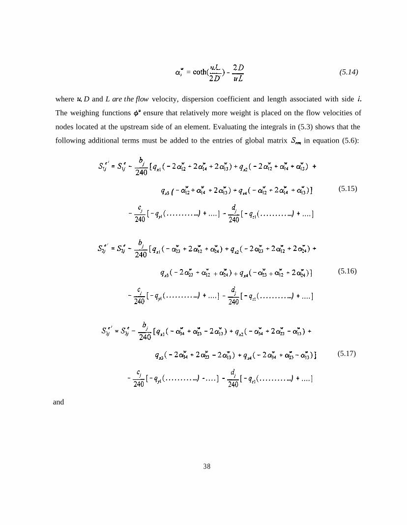
uL 20CY; = coth(_) - -20 UL

(5.14)

where u, D and L are the flow velocity, dispersion coefficient and length associated with side i.

The weighing functions 4” ensure that relatively more weight is placed on the flow velocities of

nodes located at the upstream side of an element. Evaluating the integrals in (5.3) shows that the

following additional terms must be added to the entries of global matrix S,, in equation (5.6):

s,;’ = s,; - &qJ-2 or;; +2cY;4 +24) +qJ-2c$ +a;yq +c$) +

q,3 ( - 62 + 01;4 +201;,) +4,&J-~; +2zl +cy;,)l

-&[-qy,( . . . . . . . . . ...) + . . . . ] -As-I-,,( . . . . . . . . . ...) + . . . . ]

(5.15)

s2,:’ = s,,’ - &I,,(- $3 +2cY;z +c$) +q&-2olT; +2cY;z +2c&) +

qJ-2G3 +0;;2 + 01;4) + qx4( - cc? + G2 +x4)1

-&-qy,( . . . . . . . . . ...) + . . . . ] -A-[-q,J . . . . . . . . . ...) + . . . . ]

(5.16)

s3,:’ = s3; - &p*,(-(sl4 +G -2473) +qx+sl+2G3 -4i) +

4,,<-2Qf; +243 -20;;;) +qxJ-201;4 f43 -G>l

-&[-qJ . . . . . . . . . ...) + . . . . ] -&-q,,( . . . . . . . . . ...) + . . . . ]

(5.17)

and

38

4,J - 44 + 244 -44) +q,~wo1;yq+201;4 -2421 (5.18)

A[-qJ ..,.........) + . . . . ] -2L[-qzJ . . . . . . . . . ...) + . . . . ]

5.3.3. Implementation of First-Type Boundary Conditions

Individual equations in the global matrix equation which correspond to nodes at which the

concentration is prescribed are replaced by new equations:

2imc, = Cd (5.19)

where c, is the prescribed value of the concentration at node n. This is done only when

Gaussian elimination is used to solve the matrix equation. A similar procedure as for water flow

(described in Section 4.3.4) is applied when the ORTHOMIN method is used. Because of

asymmetry of the global matrix [G], no additional manipulations are needed in the resulting

system of equations as was the case for the water flow solution.

The total material flux, Qr, through a boundary at node n consists of the dispersive flux,

Q"n 7 and the convective flux, QR:

QnT = QnD + QnA (5.20)

The dispersive boundary nodal flux is not known explicitly but must be calculated from equation

(5.4). Hence, the dispersion flux, QmD, for node n can be calculated as

j+l

QnD = - [Es;;’ +(l -+~]c,+~+ -(l -E)f; -Q;;’C” -cl (5.21)

At

The convective flux is evaluated as

39

Qff = Qncn

where the fluid flux Q, is known from the solution of the water flow equation.

5.3.4. Implementation of Third-Type Boundary Conditions

Equation (3.9) is rewritten as follows

f3D..Enj =q;n,(c-c,)!I axj

When substituted into the last term of (5.3), the boundary integral becomes

(5.22)

(5.23)

(5.24)

IN ,

The first term on the right-hand side of (5.24) represents the convective flux. This term is

incorporated into the coefficient matrix [S] of (5.4). The last term of (5.24) represents the total

material flux, which is added to the known vector v>.

At nodes where free outflow of water and its dissolved solutes takes place, the exit

concentration cO is equal to the local (nodal) concentration c,. In this case the dispersive flux

becomes zero and the total material flux through the boundary is evaluated as

Q.T = Qncn (5.25)

5.3.5. Mass Balance Calculations

The total amount of mass in the entire flow domain, or in a preselected subregion, is given

by

ORcdil=z V,&Rici + e,R,c, + OkRkck + 8,R,c,

e 4e

(5.26)

40

where eij,kl, Rij,cl and coskl represent, respectively, water

concentrations evaluated at the comer nodes of element e.

elements within the specified region.

contents, retardation factors, and

The summation is taken over all

The cumulative amounts M” and A4’ of solute removed from the flow region by zero- and

first-order reactions, respectively, are calculated as follows

whereas the cumulative amount M, of solute taken up by plant roots is given by

ScsdsZdt

(5.27)

(5.28)

(5.29)

where eR represents the elements making up the root zone.

Finally, when all boundary material fluxes, decay reactions, and root uptake mass fluxes

have been computed, the following mass balance should hold, at least theoretically, for the flow

domain as a whole:

MI-MO= ‘~QnTdt+Mo+M’ -M,I0 “r

(5.30)

where M, and MO are the amounts of solute in the flow region at times t and zero, respectively,

as calculated with (5.26), and n, represents nodes located along the boundary of the flow domain

or at internal sinks and/or sources. However, since numerical solutions are always approximate,

(5.30) will generally not be exact. The difference between the left- and right-hand sides of (5.30)

represents the absolute error, ed, in the solute mass balance. Similarly as for water flow, the

accuracy of the numerical solution for solute transport is evaluated by using the relative error,

41

erC [%], in the solute mass balance as follows

E; =100 1 EL J

ic (M,‘-M,‘l, pf”I + W’I + MI + ’

1

(5.3 1)max

dc I Qn’l GQe “r

where M,’ and A4,’ are the amounts of solute in element e at times 0 and t, respectively. Note

again that SWMS_3D does not relate the absolute error to the total amount of mass in the flow

region. Instead, the program uses as a reference the maximum value of (1) the absolute change

in element concentrations as summed over all elements, and (2) the sum of the absolute values

of all cumulative solute fluxes across the flow boundaries including those resulting from sources

and sinks in the flow domain.

5.3.6. Prevention of Numerical Oscillations

Numerical solutions of the transport equation often exhibit non-physical oscillatory

behavior and/or excessive numerical dispersion near relatively sharp concentration fronts. These

problems can be especially serious for convection-dominated transport characterized by small

dispersivities. One way to partially circumvent numerical oscillations is to use upstream weighing

as discussed in Section 5.3.2. Undesired oscillations can often be prevented also by selecting an

appropriate combination of space and time discretizations. Two dimensionless numbers may be

used to characterize the space and time discretizations. One of these is the grid Peclet number,

Pee, which defines the predominant type of the solute transport (notably the ratio of the

convective and dispersive transport terms) in relation to coarseness of the finite element grid:

4jAxiPei’ = -t9D,

(5.32)

where AX, is the characteristic length of a finite element. The Peclet number increases when the

convective part of the transport equation dominates the dispersive part, i.e., when a relatively

steep concentration front is present. To achieve acceptable numerical results, the spatial

discretization must be kept relatively fine to maintain a low Peclet number. Numerical oscillation

42

can be virtually eliminated when the local Peclet numbers do not exceed about

acceptably small oscillations may be obtained with local Peclet numbers as high as

and Pinder, 1983].

5. However,

10 [Huyakorn

A second dimensionless number which characterizes the relative extent of numerical

oscillations is the Courant number, Crf. The Courant number is associated with the time

discretization as follows

9;bCr,’ = -8RAxi

(5.33)

Three stabilizing options are used in SWMS_3D to avoid oscillations in the numerical

solution of the solute transport equation [hzz.hek and Suarez, 1993]. One option is upstream

weighing (see Section 5.3.2), which effectively eliminates undesired oscillations at relatively high

Peclet numbers. A second option for minimizing or eliminating numerical oscillations uses the

following criterion developed by Perrochet and Berod [1993]

PeCrlus =2 (5.34)

where w, is the performance index [-]. This criterion indicates that convection-dominated

transport problems having large Pe numbers can be safely simulated provided Cr is reduced

according to (5.34) [Perrochet and Berod, 1993]. When small oscillations in the solution can be

tolerated,

A

However,

w, can be increased to about 5 or 10.

third stabilizing option implemented in SWMS_3D also utilizes criterion (5.33).

instead of decreasing Cr to satisfy equation (5.33), this option introduces artificial

dispersion to decrease the Peclet number. The amount of additional longitudinal dispersivity, EL

[L], is given by [Perrochet and Berod, 1993]

< = IqlAr_D _ eDdrBRy L 141

(5.35)

The maximum permitted time step is calculated using all three options, as well as the additional

requirement that the Courant number must remain less than or equal to 1. The time step

43

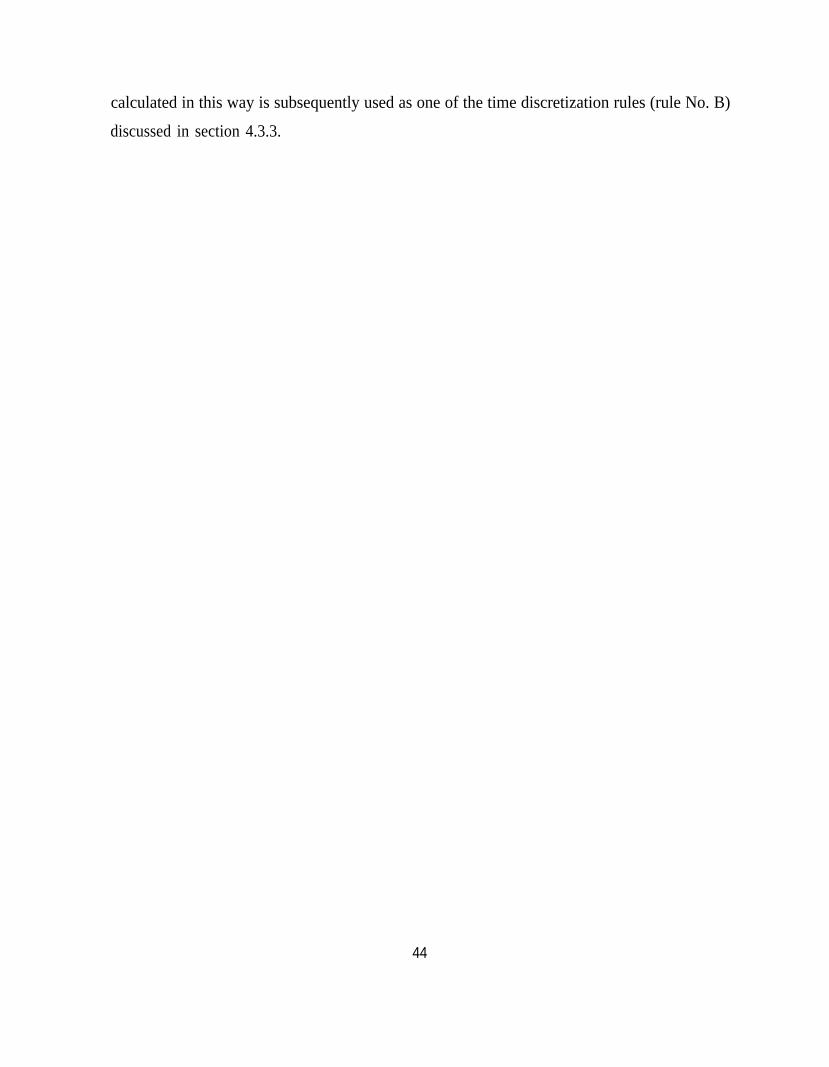
calculated in this way is subsequently used as one of the time discretization rules (rule No. B)

discussed in section 4.3.3.

44

6. PROBLEM DEFINITION

6.1. Construction of Finite Element Mesh

The finite element mesh is constructed by dividing the flow region into tetrahedral,

hexahedral and/or triangular prismatic elements (Fig. 6.1) whose shapes are defined by the

coordinates of the nodes that form the element comers. The program automatically subdivides

hexahedrals and triangular prisms into tetrahedrals which are then treated as subelements (Fig.

6.1). Two different ways are possible in SWMS_3D to subdivide the hexahedrals into

tetrahedrals, whereas six different possibilities exist for subdividing the triangular prisms into

tetrahedrals (see Fig. 6.1). Since it is important to keep the proper orientation of comer nodes

for each subelement, it is necessary to pay close attention on how the comer nodes of an element

are written into the input file.

If two neighboring hexahedral elements are subdivided in the same way (e.g., options 2a

or 2b in Figure 6.1), the newly formed edges on a common surface will cross each other, a

feature which is not allowed. Two neighboring hexahedral elements should therefore always use

both options 2a and 2b as shown in Figure 6.1, so that the newly formed edges on the common

surface will coincide. Therefore, it is necessary to give not only the comer nodes which define

an element, but also the code which specifies how a particular element is to be subdivided into

subelements. It is necessary to always realize how the neighboring elements are going to be

subdivided, and to input also the proper code specifying the subdivision. Having high flexibility

in terms of possible subdivisions into subelements is important, especially for unstructured finite

element meshes using triangular prisms. In order to overcome some of the problems related

correct definition of the comer nodes and the subdivision codes in the input file, we have

provided a separate finite element generator which may be used to generate the nodes and

elements for a hexahedral domain.

The finite element dimensions always must be adjusted to a particular problem. They

should be made relatively small in directions where large hydraulic gradients are expected.

Regions with sharp gradients are usually located in the vicinity of the internal sources or sinks,

or close to the soil surface where highly variable meteorological factors can cause fast changes

45

in pressure head. Hence, we recommend to normally use relatively small elements at and near

the soil surface. The size of elements can gradually increase with depth to reflect the generally

much slower changes in pressure heads at deeper depths. The element dimensions should also

depend upon the soil hydraulic properties. For example, coarse-textured soils having relatively

high n-values and small a-values (see Eqs. (2.11) and (2.18)) generally require a finer

discretization than fine-textured soils. We also recommend using elements having approximately

equal sizes to decrease numerical errors. No special restrictions are necessary to facilitate the soil

root zone.

6.2. Coding of Soil Types and Subregions

Soil Types - An integer code beginning with 1 and ending with NMat (the total number

of soil materials) is assigned to each soil type in the flow region. The appropriate material code

is subsequently assigned to each nodal point n of the finite element mesh.

Interior material interfaces do not coincide with element boundaries. When different

material numbers are assigned to the comer nodes of a certain element, material properties of this

element will be averaged automatically by the finite element algorithm. This procedure will

somewhat smooth soil interfaces.

A set of soil hydraulic parameters and solute transport characteristics must be specified

for each soil material. Also, the user must define for each element the principal components of

the conductivity anisotropy tensor,

systems.

as well as the angle between the local and global coordinate

As explained in Section 2.3, one additional way of changing the unsaturated soil hydraulic

properties in the flow domain is to introduce scaling factors associated with the water content,

the pressure head and the hydraulic conductivity. The scaling factors are assigned to each nodal

point n in the flow region.

Subregions - Water and solute mass balances are computed separately for each specified

subregion. The subregions may or may not coincide with the material regions. Subregions are

47

characterized by an integer code which runs from 1 to NLay (the total number of subregions).

A subregion code is assigned to each element in the flow domain.

6.3. Coding of Boundary Conditions

Flow boundary conditions were programmed in a fairly similar way as done in the

UNSATl and UNSAT2 models of Neuman [ 1972] and Neuman et al. [ 1974]. A boundary code,

Kode(n), must be assigned to each node, n. If node n is to have a prescribed pressure head

during a time step (Dirichlet boundary condition), Kode(n) must be set positive during that time

step. If the volumetric flux of water entering or leaving the system at node n is prescribed during

a time step (Neumann boundary condition), Kode(n) must be negative or zero.

Constant Boundary Conditions - The values of constant boundary conditions for a

particular node, n, are given by the initial values of the pressure head, h(n), in case of Dirichlet

boundary conditions, or by the initial values of the recharge/discharge flux, Q(n), in case of

Neumann boundary conditions. Table 6.1 summarizes the use of the variables Kode(n), Q(n) and

h(n) for various types of nodes.

Table 6.1. Initial settings of Kode(n), Q(n), and h(n) for constant boundary conditions.

Node Type

Internal; not sink/source

Internal; sink/source(Dirichlet condition)

Internal; sink/source(Neumann condition)

Impermeable Boundary

Specified Head Boundary

Specified Flux Boundary

Kode(n) Q(n) h(n)

0 0.0 Initial Value

1 0.0 Prescribed

-1 Prescribed Initial Value

0 0.0 Initial Value

1’ 0.0 Prescribed

-1: Prescribed Initial Value

+ 6 may also be used* -6 may also be used

48

Variable Boundary Conditions - Three types of variable boundary conditions can be

imposed:

1. Atmospheric boundary conditions for which Kode(n)=_+4,

2. Variable pressure head boundary conditions for which Kode(n) = +3, and

3. Variable flux boundary conditions for which Kode(n) = -3.

These conditions can be specified along any part of the boundary. It is not possible to specify

more than one time-dependent boundary condition for each type. Initial settings of the variables

Kode(n), Q(n) and h(n) for the time-dependent boundary conditions are given in Table 6.2.

Table 6.2. Initial settings of Kode(n), Q(n), and h(n) for variable boundary conditions.

Node Type Kode( n) Q(n) h(n)

Atmospheric Boundary

Variable Head Boundary

Variable Flux Boundary

- 4

+3

- 3

0.0

0.0

0.0

Initial Value

Initial Value

Initial Value

Atmospheric boundary conditions are implemented when Kode(n)=+4, in which case time-

dependent input data for the precipitation, Prec, and evaporation, rSoil, rates must be specified

in the input file ATMOSPH.IN. The potential fluid flux across the soil surface is determined

by rAtm= rSoil-Prec. The actual surface flux is calculated internally by the program. Two

limiting values of the surface pressure head must be provided: hCritS which specifies the

maximum allowed pressure head at the soil surface (usually O.O), and hCritA which specifies the

minimum allowed surface pressure head (defined from equilibrium conditions between soil water

and atmospheric vapor). The program automatically switches the value of Kode(n) from -4 to

+4 if one of these two limiting points is reached. Table 6.3 summarizes the use of the variables

rAtrn, hCritS and hCritA during program execution. Width(n) in this table denotes the surface

area of the boundary segment associated with node n.

49

Table 6.3. Definition of the variables Kode(n), Q(n) and h(n)when an atmospheric boundary condition is applied.

Kode( n) Q(n) h(n) Event

-4

+4

-Width(n)*rAtm Unknown

Unknown hCritA

rAtm=rSoil-Prec

Evaporation capacityis exceeded

+4 Unknown hCritS Infiltration capacityis exceeded

Variable head and flux boundary conditions along a certain part of the boundary are

implemented when Kode(n)=+3 and -3, respectively. In that case, the input file ATMOSPH.IN

must contain the prescribed time-dependent values of the pressure head, ht, or the flux, rt,

imposed along the boundary. The values of ht or rt are assigned to particular nodes at specified

times according to rules given in Table 6.4.

Table 6.4. Definition of the variables Kode(n), Q(n) and h(n)when variable head or flux boundary conditions are applied.

Node Type Kode(n) Q(n) h(n)

Variable Head Boundary

Variable Flux Boundary

+3

-3

Unknown

-Width(n)*rt

ht

Unknown

Water Uptake by Plant Roots - The program calculates the rate at which plants extract

water from the soil root zone by evaluating the term D (equation (4.9)) in the finite element

formulation. The code requires that Kode(n) be set equal to 0 or negative for all nodes in the

root zone. Values of the potential transpiration rate, rRoot, must be specified at preselected times

in the input file ATMOSPH.IN. Actual transpiration rates are calculated internally by the

program as discussed in Section 2.2. The root uptake parameters are taken from input file

50

SELECTOR.IN. Values of the function Beta(n), which describes the potential water uptake

distribution over the root zone (equation (2.5)), must be specified for each node in the flow

domain (see the description of input Block H in Table 8.8 of Section 8). All parts of the flow

region where Beta(n)>0 are treated as the soil root zone.

Deep Drainage fromm the Soil Profile - Vertical drainage, q(h), across the lower boundary

of the soil profile is sometimes approximated by a flux which depends on the position of

groundwater level (e.g., Hopmans and Stricker, 1989). If available, such a relationship can be

implemented in the form of a variable flux boundary condition for which Kode(n)= -3. This

boundary condition is implemented in SWMS_3D by setting the logical variable qGWLF in the

input file ATMOSPH.IN equal to “true.” The discharge rate Q(n) assigned to node n is

determined in the program as Q(n)=- Width(n)*q(h) where h is the local value of the pressure

head, and q(h) is given by

q(h) = -Aqhexp(Bqh jh-GWLOL I> (6.1)

where A, and Bq,, are empirical parameters which must be specified in the input file

ATMOSPH.IN, together with GWLOL which represents the reference position of the groundwater

level (usually set equal to the z-coordinate of the soil surface).

Free Drainage - Unit vertical hydraulic gradient boundary conditions can be implemented

in the form of a variable flux boundary condition for which Kode(n)= -3. This boundary

condition is implemented in SWMS_3D by setting the logical variable FreeD in the input file

SELECTOR.IN equal to “true.“. The program determines the discharge rate Q(n) assigned to

node n as Q(n)= -Width(n)*K(h), where h is the local value of the pressure head, and K(h) is the

hydraulic conductivity corresponding to this pressure head.

Seepage Faces - The initial settings of the variables Kode(n), Q(n) and h(n) for nodes

along a seepage face are summarized in Table 6.5. All potential seepage faces must be identified

before starting the numerical simulation. This is done by providing a list of nodes along each

51

potential seepage face (see input Block E as defined in Table 8.5 of Section 8).

Table 6.5. Initial setting of Kode(n), Q(n), and h(n) for seepagefaces.

Node Type Kode(n) Q(n) h(n)

Seepage Face(initially saturated)

Seepage Face(initially unsaturated)

+2

- 2

0.0

0.0

0.0

Initial Value

Drains - Table 6.6 summarizes the initial settings of the variables Kode(n),

for nodes representing drains. All drains must be identified before starting the numerical

simulation. This is done by providing a list of nodes representing drains, together with a list of

elements around each drain whose hydraulic conductivities are to be adjusted according to

discussion in Section 4.3.7 (see also input Block F as defined in Table 8.6 of Section 8).

Table 6.6. Initial setting of Kode(n), Q(n), and h(n) for drains.

Node Type

Drain(initially saturated)

Drain(initially unsaturated)

Kode(n) Q(n) h(n)

+5 0.0 0.0

- 5 0.0 Initial Value

Solute Transport Boundary Conditions. The type of boundary condition to be invoked

for solute transport is specified by the input variable KodCB. A positive sign of this variable

means that a first-type boundary condition will be used. When KodCB is negative, SWMS_3D

selects a third-type boundary condition when the calculated water flux is directed into the region,

or a second-type boundary condition when the water flux is zero or directed out of the region.

52

One exception to these rules occurs for atmospheric boundary conditions when Kode(n)=+4 and

Q(n)<O. SWMS_3D assumes that solutes cannot leave the flow region across atmospheric

boundaries. The solute flux in this situation becomes zero, i.e., c,=O in equation (5.23). Cauchy

and Neumann boundary conditions are automatically applied to internal sinks/sources depending

upon the direction of water flow. The dependence (or independence) of the solute boundary

conditions on time or the system is then still defined through the variable Kode(n) as discussed

above.

Although SWMS_3D can implement frost-type boundary conditions, we recommend users

to invoke third-type conditions where possible. This is because third-type conditions, in general,

are physically more realistic and preserve solute mass in the simulated system (e.g., van

Genuchten and Parker [ 1984]; Leij et al. [1991]).

For the user’s convenience, Table 6.7 summarizes possible values of the different

boundary codes and their association with specific water flow and solute transport boundary

conditions.

6.4. Program Memory Requirements

One single parameter statement is used at the beginning of the code to define the problem

dimensions. All major arrays in the program are adjusted automatically according to these

dimensions. This feature makes it possible to change the dimensions of the problem to be

simulated without having to recompile all program subroutines. Different problems can be

investigated by changing the dimensions in the parameter statement at the beginning of the main

program, and subsequently linking all previously compiled subroutines with the main program

when creating an executable file. Table 6.8 lists the array dimensions which must be defined in

the parameter statement.

53

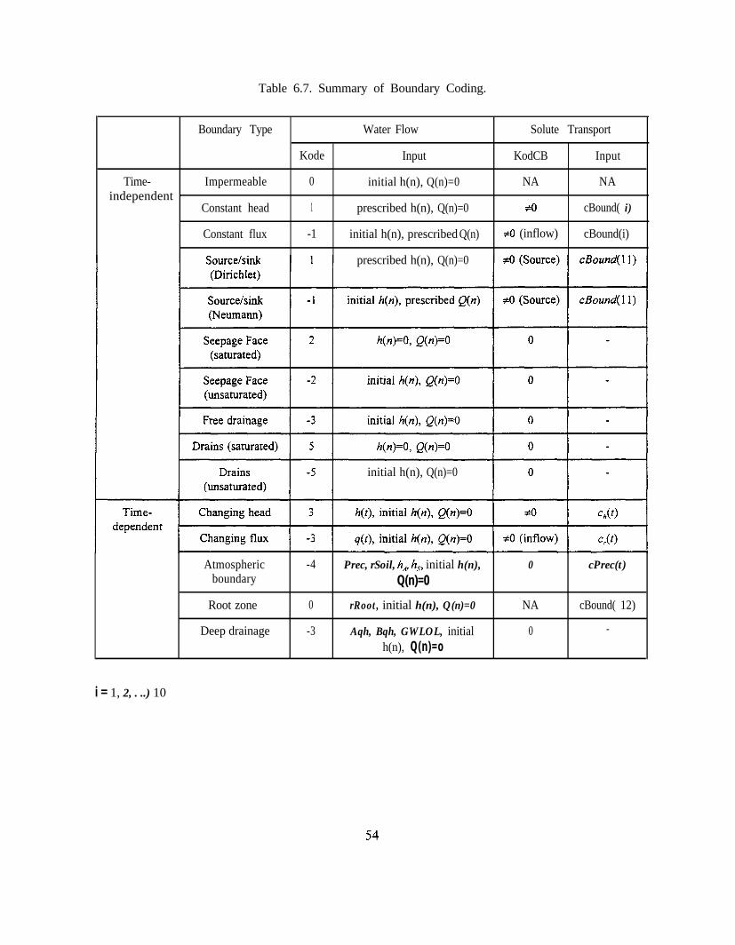
Table 6.7. Summary of Boundary Coding.

Boundary Type Water Flow Solute Transport

Kode Input KodCB Input

Time- Impermeable 0 initial h(n), Q(n)=0 NA NAindependent .

Constant head 1 prescribed h(n), Q(n)=0 #O cBound( i)

Constant flux -1 initial h(n), prescribed Q(n) $0 (inflow) cBound(i)

prescribed h(n), Q(n)=0

initial h(n), Q(n)=0

Atmospheric -4 Prec, rSoil, h,, h,, initial h(n), 0 cPrec(t)boundary Q(n)=0

Root zone 0 rRoot, initial h(n), Q(n)=0 NA cBound( 12)

Deep drainage -3 Aqh, Bqh, GWLOL, initial 0 -

h(n), Q(n)=o

i = 1, 2, . ..) 10

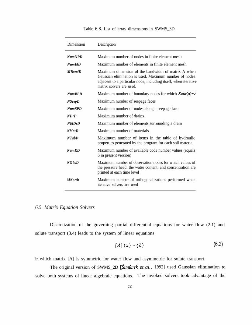
Table 6.8. List of array dimensions in SWMS_3D.

Dimension

NumNPD

NumElD

MBandD

NumBPD

NSeepD

NumSPD

NDrD

NElDrD

NMatD

NTabD

NumKD

NObsD

MNorth

Description

Maximum number of nodes in finite element mesh

Maximum number of elements in finite element mesh

Maximum dimension of the bandwidth of matrix A whenGaussian elimination is used. Maximum number of nodesadjacent to a particular node, including itself, when iterativematrix solvers are used.

Maximum number of boundary nodes for which Kode(n)+O

Maximum number of seepage faces

Maximum number of nodes along a seepage face

Maximum number of drains

Maximum number of elements surrounding a drain

Maximum number of materials

Maximum number of items in the table of hydraulicproperties generated by the program for each soil material

Maximum number of available code number values (equals6 in present version)

Maximum number of observation nodes for which values ofthe pressure head, the water content, and concentration areprinted at each time level

Maximum number of orthogonalizations performed wheniterative solvers are used

6.5. Matrix Equation Solvers

Discretization of the governing partial differential equations for water flow (2.1) and

solute transport (3.4) leads to the system of linear equations

(6.2)

in which matrix [A] is symmetric for water flow and asymmetric for solute transport.

The original version of SWMS_2D [,.%nGnek et al., 1992] used Gaussian elimination to

solve both systems of linear algebraic equations. The invoked solvers took advantage of the

cc

banded nature of the coefficient matrices and, in the case of water flow, of the symmetric

properties of the matrix. Such direct solution methods have several disadvantages as compared

to iterative methods. Direct methods require a fixed number of operations (depending upon the

size of the matrix) which increases approximately by the square of the number of nodes

[Mendoza et. al., 1991]. Iterative methods, on the other hand, require a variable number of

repeated steps which increase at a much smaller rate (about 1.5) with the size of a problem

[Mendoza et al., 1991]. A similar reduction also holds for the memory requirement since

iterative methods do not require the storage of non-zero matrix elements. Memory requirements,

therefore, increase at a much smaller rate with the size of the problem when iterative solvers are

used [Mendoza et al., 1991]. Round-off errors also represent less of a problem for iterative

methods as compared to direct methods. This is because round-off errors in iterative methods

are self-correcting [Letniowski, 1989]. Finally, for time-dependent problems, a reasonable

approximation of the solution (i.e., the solution at the previous time step) exists for iterative

methods, but not for direct methods [Letniowski, 1989]. In general, direct methods are more

appropriate for relatively small problems, while iterative methods are more suitable for larger

problems.

Many iterative methods have been used in the past for handling large sparse matrix

equations. These methods include Jacobi, Gauss-Seidel, alternating direction implicit (ADI),

block successive over-relaxation (BSSOR), successive line over-relaxation (SLOR), and strongly

implicit procedures (SIP), among others [Letniowski, 1989]. More powerful preconditioned

accelerated iterative methods, such as the preconditioned conjugate gradient method (PCG) [Behie

and Vinsome, 1982], were introduced more recently. Sudicky and Huyakorn [1991] gave three

advantages of the PCG procedure as compared to other iterative methods: PCG can be readily

applied to finite element methods with irregular grids, the method does not require iterative

parameters, and PCG usually outperforms its iterative counterparts for situations involving

relatively stiff matrix conditions.

The current version 1.0 of SWMS_3D implements both direct and iterative methods for

solving the system of linear algebraic equations given by (6.2). Depending upon the size of

matrix [A], we use either direct Gaussian elimination or the preconditioned conjugate gradient

56

method [Mendoza et al., 1991) for water flow and the ORTHOMIN (preconditioned conjugate

gradient squared) procedure [Mendoza et al., 1991] for solute transport. Gaussian elimination

is used if either the bandwidth of matrix [A] is smaller than 20, or the total number of nodes is

smaller than 500. The iterative methods used in SWMS_3D were adopted from the ORTHOFEM

software package of Mendoza et al. [ 1991].

The preconditioned conjugate gradient and ORTHOMIN methods consist of two essential

parts: initial preconditioning, and iterative solution with either conjugate gradient or ORTHOMIN

acceleration [Mendoza et al., 1991]. Incomplete lower-upper (ILU) preconditioning is used in

ORTHOFEM when matrix [A] is factorized into lower and upper triangular matrices by partial

Gaussian elimination. The preconditioned matrix is subsequently repeatedly inverted using

updated solution estimates to provide a new approximation of the solution. The

orthogonalization-minimization acceleration technique is used to update the solution estimate.

This technique insures that the search direction for each new solution is orthogonal to the

previous approximate solution, and that either the norm of the residuals (for conjugate gradient

acceleration [Meijerink and van der Vorst, 1981]) or the sum of squares of the residuals (for

ORTHOMIN [Behie and Vinsome, 1982]) is minimized. More details about the two methods is

given in the user’s guide of ORTHOFEM [Mendoza et al., 1991] or in Letniowski [ 1989].

Letniowski [1989] also gives a comprehensive review of accelerated iterative methods, as well

as of different preconditioning techniques.

57

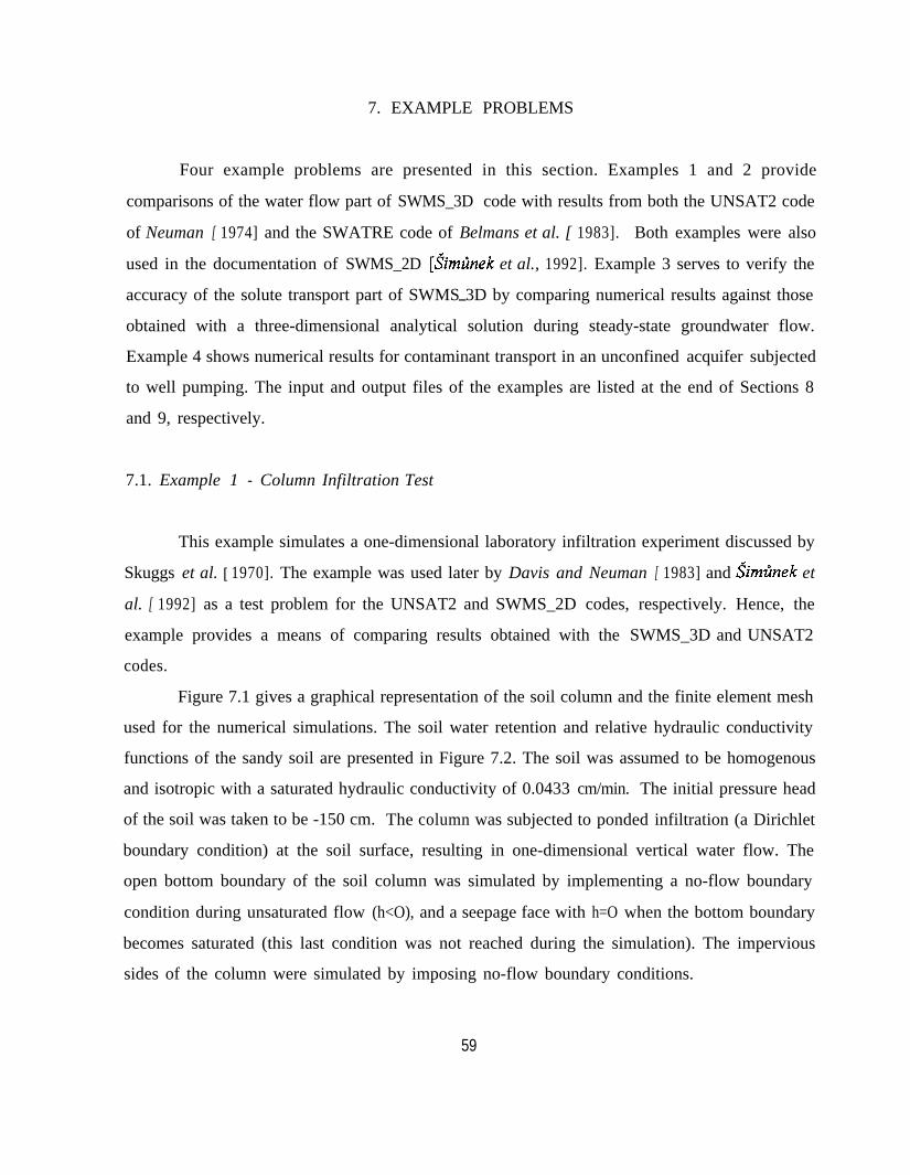
7. EXAMPLE PROBLEMS

Four example problems are presented in this section. Examples 1 and 2 provide

comparisons of the water flow part of SWMS_3D code with results from both the UNSAT2 code

of Neuman [ 1974] and the SWATRE code of Belmans et al. [ 1983]. Both examples were also

used in the documentation of SWMS_2D [Simzhek et al., 1992]. Example 3 serves to verify the

accuracy of the solute transport part of SWMS 3D by comparing numerical results against those-

obtained with a three-dimensional analytical solution during steady-state groundwater flow.

Example 4 shows numerical results for contaminant transport in an unconfined acquifer subjected

to well pumping. The input and output files of the examples are listed at the end of Sections 8

and 9, respectively.

7.1. Example 1 - Column Infiltration Test

This example simulates a one-dimensional laboratory infiltration experiment discussed by

Skuggs et al. [ 1970]. The example was used later by Davis and Neuman [ 1983] and &mzhek et

al. [ 1992] as a test problem for the UNSAT2 and SWMS_2D codes, respectively. Hence, the

example provides a means of comparing results obtained with the SWMS_3D and UNSAT2

codes.

Figure 7.1 gives a graphical representation of the soil column and the finite element mesh

used for the numerical simulations. The soil water retention and relative hydraulic conductivity

functions of the sandy soil are presented in Figure 7.2. The soil was assumed to be homogenous

and isotropic with a saturated hydraulic conductivity of 0.0433 cm/min. The initial pressure head

of the soil was taken to be -150 cm. The column was subjected to ponded infiltration (a Dirichlet

boundary condition) at the soil surface, resulting in one-dimensional vertical water flow. The

open bottom boundary of the soil column was simulated by implementing a no-flow boundary

condition during unsaturated flow (h<O), and a seepage face with h=O when the bottom boundary

becomes saturated (this last condition was not reached during the simulation). The impervious

sides of the column were simulated by imposing no-flow boundary conditions.

59

217

221

20

24

Fig. 7.1. Flow system and finite element mesh for example 1.

The simulation was carried out for 90 min, which corresponds to the total time duration

of the experiment. Figure 7.3 shows the calculated instantaneous (qJ and cumulative (I,)

infiltration rates simulated with SWMS_3D. Notice that the calculated results agreed closely with

those obtained by Davis and Neuman [1983] using their UNSAT2 code. The results obtained

with SWMS_3D code were essentially identical with those calculated with SWMS_2D.

60

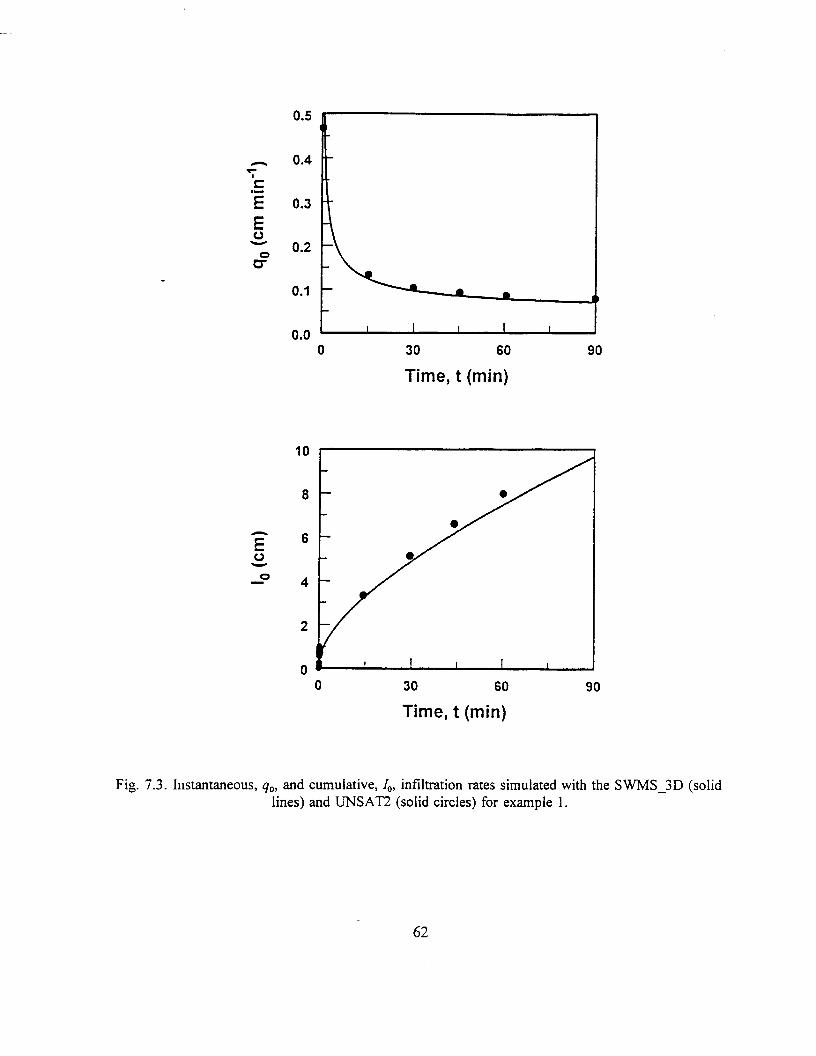
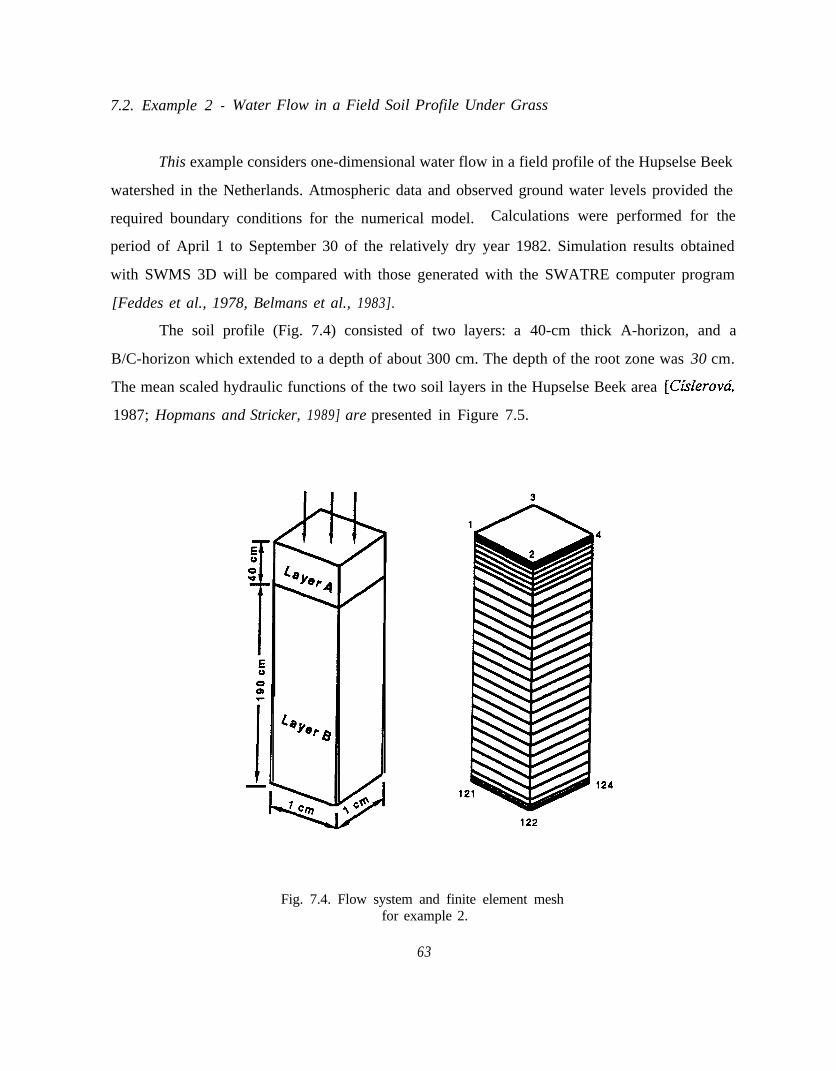
7.2. Example 2 - Water Flow in a Field Soil Profile Under Grass

This example considers one-dimensional water flow in a field profile of the Hupselse Beek

watershed in the Netherlands. Atmospheric data and observed ground water levels provided the

required boundary conditions for the numerical model. Calculations were performed for the

period of April 1 to September 30 of the relatively dry year 1982. Simulation results obtained

with SWMS 3D will be compared with those generated with the SWATRE computer program

[Feddes et al., 1978, Belmans et al., 1983].

The soil profile (Fig. 7.4) consisted of two layers: a 40-cm thick A-horizon, and a

B/C-horizon which extended to a depth of about 300 cm. The depth of the root zone was 30 cm.

The mean scaled hydraulic functions of the two soil layers in the Hupselse Beek area [Cislerovb,

1987; Hopmans and Stricker, 1989] are presented in Figure 7.5.

Fig. 7.4. Flow system and finite element meshfor example 2.

63

The soil surface boundary conditions involved actual precipitation and potential

transpiration rates for a grass cover. The surface fluxes were incorporated by using average daily

rates distributed uniformly over each day. The bottom boundary condition consisted of a

prescribed drainage flux - groundwater level relationship, q(h), as given by equation (6.1). The

groundwater level was initially set at 55 cm below the soil surface. The initial moisture profile

was taken to be in equilibrium with the initial ground water level.

Figure 7.6 presents input values of the precipitation and potential transpiration rates.

Calculated cumulative transpiration and cumulative drainage amounts as obtained with the

SWMS_3D and SWATRE codes are shown in Figure 7.7. The pressure head at the soil surface

and the arithmetic mean pressure head of the root zone during the simulated season are presented

in Figure 7.8. Finally, Figure 7.9 shows variations in the calculated groundwater level with time.

Again, the results obtained with SWMS_3D code are almost identical with those calculated with

SWMS_2D.

64

182

Time, t (day)

273

Fig. 7.9. Location of the groundwater table versus time for example 2 as simulated with theSWMS_3D (solid line) and SWATRE (solid circles) computer programs.

7.3. Example 3 - Three-Dimensional Solute Transport

This example was used to verify the mathematical accuracy of the solute transport part

of SWMS_3D. Leij et al. [1991] published several analytical solutions for three-dimensional

dispersion problems. One of these solutions holds for solute transport in a homogeneous,

isotropic porous medium during steady-state unidirectional groundwater flow (Figure 7.10). The

solute transport equation (3.4) for this situation reduces to

R a~ _D 8~ +D a% +D a% acdt- Tax Tdy’

- -v-L aZl a2

-pLC+X (7.1)

where X and p are a zero- and first-order degradation constants, respectively; D, and Dr are the

longitudinal and transverse dispersion coefficients, respectively; v (= q1/6) is the average pore

water velocity in the flow direction, and z is the spatial coordinate parallel to the direction of

flow, while x and y are the spatial coordinates perpendicular to the flow direction. The initially

69

solute-free medium is subjected to a solute source, c,, of unit concentration. The rectangular

surface source has dimensions 2a and 2b along the inlet boundary at z=O, and is located

symmetrically about the coordinates x=0 and y=O (Figure 7.10). The transport region of interest

is the half-space (~20; -a&clco, -OO+JSOO). The boundary conditions may be written as:

c (X,Y, o,r> = c, -aSxla, -b<ySb

4X,Y,OJ) = 0 other values of x, y

lima’- = oz--ra a 2

1imaC = 0x+M ax

lim2 =Or- aY

The analytical solution of the above transport problem is [Leij and Bradford, 1994]

r

II11 dr +

1

(7.2)

(7.3)

where P(t) = 0 if t<to and P(t) = t-t, if t>r,, and where t,, is the duration of solute pulse. The

input transport parameters for two simulations are listed in Table 7.1. The width of the source

was assumed to be 100 m in both the x and y directions. Because of symmetry, calculations were

carried out only for part of the transport domain where x20, ~20 and ~0.

70

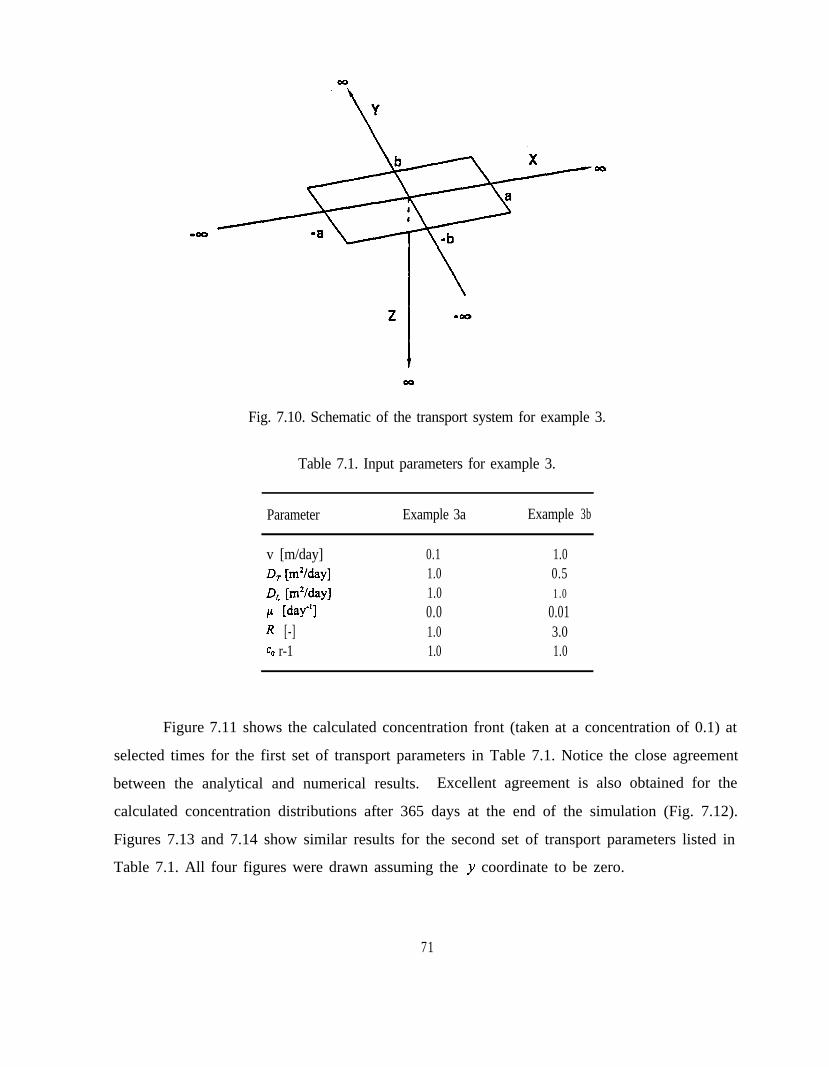
Fig. 7.10. Schematic of the transport system for example 3.

Table 7.1. Input parameters for example 3.

Parameter Example 3a Example 3b

v [m/day] 0.1 1.0D, [m’/day] 1.0 0.5DL [m’lday] 1.0 1.0

P [day? 0.0 0.01R [-] 1.0 3.0co r-1 1.0 1.0

Figure 7.11 shows the calculated concentration front (taken at a concentration of 0.1) at

selected times for the first set of transport parameters in Table 7.1. Notice the close agreement

between the analytical and numerical results. Excellent agreement is also obtained for the

calculated concentration distributions after 365 days at the end of the simulation (Fig. 7.12).

Figures 7.13 and 7.14 show similar results for the second set of transport parameters listed in

Table 7.1. All four figures were drawn assuming the y coordinate to be zero.

71

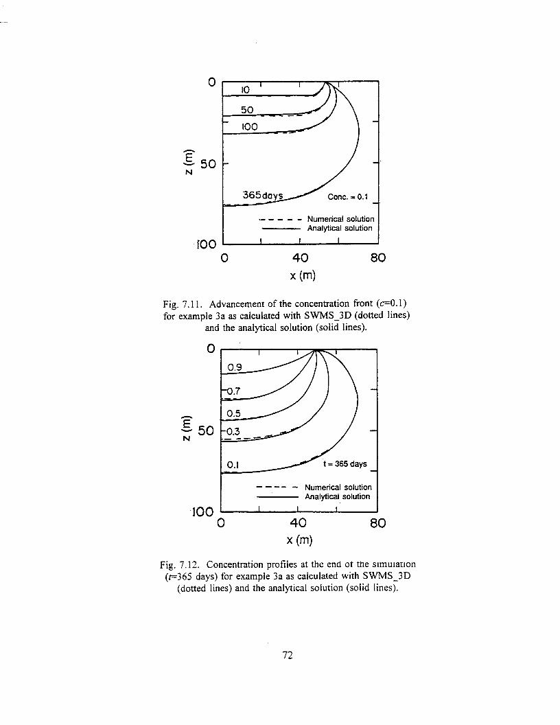
7.4. Example 4 - Contaminant Transport From a Waste Disposal Site

This test problem concerns contaminant transport from a waste disposal site (or possibly

a landfill) into a unconfined aquifer containing a pumping well downgradient of the disposal site

as shown in Figure 7.15. Water was assumed to infiltrate from the disposal site into the

unsaturated zone under zero-head ponded conditions. The concentration of the contaminant

leaving the disposal site was taken to be 1 .O during the first 50 days, and zero afterwards. The

waste disposal site itself had lateral dimensions of 10 x 40 m*. Initially, the water table decreased

from a height of 28 m above the base of the aquifer at the left-hand side (Figure 7.15) to 26 m

on the right-hand side of the flow domain. The initial pressure head in the unsaturated zone was

assumed to be at equilibrium with the initial water table, i.e., no vertical flow occurred. The

transport experiment started when the water table in the fully penetrated well at x = 170 m @=

0) was suddenly lowered to a height of 18 m above the bottom of the unconfined aquifer. We

assumed that at that same time (t = 0) infiltration started to occur from the disposal site.

Prescribed hydraulic head conditions h + z = 28 m and h + z = 26 m were imposed along the left-

hand (x = 0) and right-hand (X = 260 m) side boundaries (-50 I y I 50 m). A prescribed

hydraulic head condition of h + z = 18 m was used to represent the well along a vertical below

the water table (z I 18) at x = 170 m and y = 0 m, while a seepage face was defined at that

location along the vertical above the water table (z > 18). No-flow conditions were assumed

along all other boundaries, including the soil interface. Hydraulic and transport parameters used

in the analysis are listed in Table 7.2. We selected the retention hydraulic parameters for a

coarse-textured soil with a relatively high saturated hydraulic conductivity, K,, in order to test the

SWMS_3D code for a comparatively difficult numerical problem.

Because of symmetry about the y axis, only half of the flow region was simulated. The

solution domain defined by 0 < x I 260, 0 I y I 50, and 0 I z I 38 m was discretized into a

rectangular grid comprised of 10560 elements and 12144 nodes (Figure 7.16). Nodal spacings

were made relatively small in regions near the disposal site and near the pumping well where the

highest head gradients and flow velocities were expected. The variably saturated flow problem

was solved using SWMS 3D assuming an iteration head tolerance of 0.01 m and a water content-

74

Table 7.2. Input parameters for example 4.

Hydraulic Parameters I Transport Parameters

fl, =e, =o, I 0.450 I P [kg/m’1 I 1400

e,=e, I 0.05 I D,, [m*/day] I 0.01

K, =K, [m/day] 5.0 I DL [m] 1.0

a [I/m]

n [-]

4.1

2.0

DT [m]

k [m’@l

P, [l/day]

pS [ 1 /day]

yy [1/day]

0.25

0.0

0.0

0.0

0.0

I yx [l/day] I 0.0

I CO I 1.0

tolerance of 0.0001.

Computed water table elevations are plotted in Figure 7.17a and 7.17b along longitudinal

o/-O) and transverse (~‘170 m) planes through the pumping well, respectively. The results show

a relatively strong direct interaction between the infiltrating water and the saturated zone after

only a short period of time; water flow reached approximately steady state about 1.5 days after

the experiment started. The velocity field and streamlines in a longitudinal section through the

pumping well are presented in Figure 7.18. Note that the length of the seepage face along the

well was determined to be approximately 5 meters. The calculated well discharge rate for the

fixed water table (z = 18 m) was calculated to be 39.6 m3/day. A concentration contour plot (c

= 0.1) is presented in Figure 7.19. This figure shows that contaminant transport was strongly

affected by well pumping. Note that although the contaminant source was located 10 m above

the initial groundwater table, and 150 m upgradient of the pumping well, the solute reached the

pumping well after only 200 days of pumping. Figure 7.20 gives a two-dimensional view of

calculated concentration distributions at several times in a horizontal plane (Z = 20 m).

76

Finally, Figure 7.21 presents solute breakthrough curves observed at observation node 1

(;r=40m,z=32m),node2(x=150m,z=24m),node3(x=170m,z=18m),andnode

4 (X = 200 m, z = 20 m). These observation nodes are all on a vertical cross-section 0, = 0) as

shown in Figure 7.15b. Notice that the breakthrough curves differ considerably in shape and

especially peak concentrations. Although the breakthrough curve at observation node 1

immediately below the disposal site was very steep, no numerical oscillations were observed here.

This shows that SWMS_3D is able to solve the present solute transport problem involving sharp

concentration distributions without generating non-physical oscillations. However, the efficiency

of the numerical simulation for this example was limited by the need for relatively small time

steps so as to satisfy the grid Courant criterion (Section 5.3.6). Although water flow had reached

approximately steady-state within less than 2 days, the time step for the solute transport problem

was only 0.073 day because of relatively large flow velocities near the well.

Fig. 7.16. Finite element mesh for example 4.

77

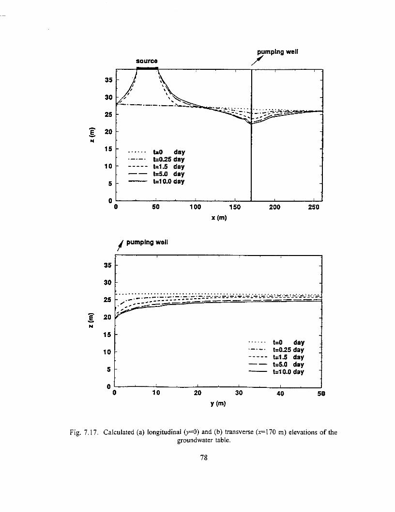
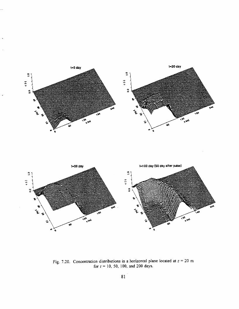
8. INPUT DATA

The input data for SWMS_3D are given in three separate input files. These input files

consist of one or more input blocks identified by the letters from A through K. The input files

and blocks must be arranged as follows:

SELECTOR.INA. Basic InformationB. Material InformationC. Time InformationD. Root Water Uptake InformationE. Seepage InformationF. Drainage InformationG. Solute Transport Information

GRID.INH. Nodal InformationI. Element InformationJ. Boundary Geometry Information

ATMOSPH.INK. Atmospheric Information

The various input blocks are described in detail in Section 8.1, while Section 8.2 lists the

actual input files for examples 1 through 4 discussed in Section 7. The output files for these

examples are discussed in Section 9.

8.1. Description of Data Input Blocks

Tables 8.1 through 8.11 describe the data required for each input block. All data are read

in using list-directed formatting (free format). Comment lines are provided at the beginning of,

and within, each input block to facilitate, among other things, proper identification of the function

of the block and the input variables. The comment lines are ignored during program execution;

hence, they may be left blank but should not be omitted. All input files must be placed in the

directory SWMS_3D.IN. The program assumes that all input data are specified in a consistent

set of units for mass M, length L, and time T.

83

Most of the information in Tables 8.1 through 8.11 should be self-explanatory. Table 8.8

(Block H) is used to define, among other things, the nodal coordinates and initial conditions for

the pressure head and the concentration. One short-cut may be used when generating the nodal

coordinates. The short-cut is possible when two nodes (e.g., N, and N2), not adjacent to each

other, are located along a transverse line such that N2 is greater than N,+l. The program will

automatically generate nodes between N, and N2, provided all of the following conditions are met

simultaneously: (1) all nodes along the transverse line between nodes N, and N2 are spaced at

equal intervals, (2) values of the input variables hNew(n), Beta(n), Axz(n), Bxz(n), Dxz(n), and

Conc(n) vary linearly between nodes N, and N,, and (3) values of Kode(n), Q(n) and MatNum(n)

are the same for all n = N,, N,+l,..., N,-1 (see Table 8.8).

A similar short-cut is possible when generating the elements in Block I (Table 8.9).

Consider two elements, E, and E2, between two transverse lines such that E2 is greater than E,.

The program requires input data only for element E, (i.e., data for elements E,+l through E2 may

be omitted), provided the following two conditions are met simultaneously: (1) all elements

between E, and E2 are hexahedrals, including E, and E,, and (2) all elements, E,,...., E,, are

assigned the same values of Cosll(e), Cos22(e), (%33(e), Cos12(e), Cos13(e), (%23(e),

Co&l(e), Con42(e), ConA3(e), and LayNum(e) as defined in Table 8.9.

To overcome problems with definition of finite elements and their comer nodes in input

file GRIDIN, we have provided a separate finite element generator GENER3 which generates

the nodes and elements for a hexahedral domain. Table 8.12 shows how the input file for the

finite element mesh generator GENER3 is constructed. The resulting file GRID.IN can be

modified using any word- or data-processing software.

84

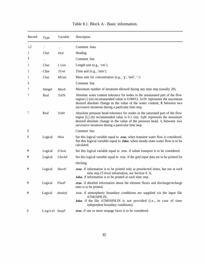
Table 8.1. Block A - Basic information.

Record Type Variable Description

1,2

3

4

5

5

5

6

7

7

-

Char

_

Char

- Char

Char

Integer

Real

7 Real TolH

8

9

9 Logical SeepF

Logical

Logical

Logical

Logical

Logical

Logical

_

Hed

L Unit

TUnit

MUnit

MaxIt

TolTh

lWat

lChem

CheckF

ShortF

FluxF

Atmlnf

Comment lines.

Heading.

Comment line.

Length unit (e.g., ‘cm’).

Time unit (e.g., ‘min’).

Mass unit for concentration (e.g., ‘g’, ‘mol’, ‘-‘).

Comment line.

Maximum number of iterations allowed during any time step (usually 20).

Absolute water content tolerance for nodes in the unsaturated part of the flowregion [-] (its recommended value is 0.0001). TolTh represents the maximumdesired absolute change in the value of the water content, 8, between twosuccessive iterations during a particular time step.

Absolute pressure head tolerance for nodes in the saturated part of the flowregion [L] (its recommended value is 0.1 cm). TofH represents the maximumdesired absolute change in the value of the pressure head, h, between twosuccessive iterations during a particular time step.

Comment line.

Set this logical variable equal to .true. when transient water flow is considered.Set this logical variable equal to .false. when steady-state water flow is to becalculated.

Set this logical variable equal to .true. if solute transport is to be considered.

Set this logical variable equal to .true. if the grid input data are to be printed for

checking.

.true. if information is to be printed only at preselected times, but not at eachtime step (T-level information, see Section 9. l),

.false. if information is to be printed at each time step.

.true. if detailed information about the element fluxes and discharge/rechargerates is to be printed.

.true. if atmospheric boundary conditions are supplied via the input fileATMOSPH.IN,

.false. if the file ATMOSPH.IN is not provided (i.e., in case of timeindependent boundary conditions).

.true. if one or more seepage faces is to be considered.

85

Table 8.1. (continued)

Record Type VariabIe Description

9 Logical FreeD Set this logical variable equal to .true. if a unit vertica1 hydraulic gradientboundary condition (free drainage) is used at the bottom boundary. Otherwiseset equal to .false. .

9 Logical DrainF Set this logical variable equal to .true. if a dram is to be simulated by means ofboundary condition. Otherwise set equal to .false. . Section 4.3.7 explains howtile drains can be represented as boundary conditions in a regular finite elementmesh.

86

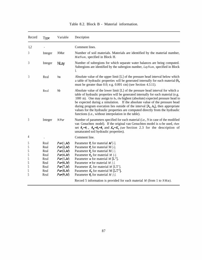
Table 8.2. Block B - Material information.

Record Type Variable Description

I,2 -

3 Integer

3 Integer

3 Real ha

Real

3 Integer

4 _

5 Real5 Real5 Real5 Real5 Real5 Real5 Real5 Real5 Real

NMat

NLay

hb

NPar

Comment lines.

Number of soil materials. Materials are identified by the material number,MatNum, specified in Block H.

Number of subregions for which separate water balances are being computed.Subregions are identified by the subregion number, LayNum, specified in BlockI.

Absolute value of the upper limit [L] of the pressure head interval below whicha table of hydraulic properties will be generated internally for each material (h,must be greater than 0.0; e.g. 0.001 cm) (see Section 4.3.11).

Absolute value of the lower limit [L] of the pressure head interval for which atable of hydraulic properties will be generated internally for each material (e.g.1000 m). One may assign to hb, the highest (absolute) expected pressure head tobe expected during a simulation. If the absolute value of the pressure headduring program execution lies outside of the interval [ho, hb], then appropriatevalues for the hydraulic properties are computed directly from the hydraulicfunctions (i.e., without interpolation in the table).

Number of parameters specified for each material (i.e., 9 in case of the modifiedvan Genuchten model). If the original van Genuchten model is to be used, thenset e,=e, ,, e,=tJ,=e, and K,=K, (see Section 2.3 for the description ofunsaturated soil hydraulic properties).

Comment line.

Parameter 8, for material M [-].Parameter e, for material M [-].Parameter e, for material M [ - ] .Parameter 8, for material M [-].Parameter 01 for material M [L-l].Parameter n for material M [-].Parameter KS for material M [LT’].Parameter Kk for material M [LT’].Parameter f$ for material M [-].

Record 5 information is provided for each material M (from 1 to NMat).

87

Table 8.3. Block C - Time information.

Record Type Variable Description

I,2

3

-

Real

3 Real

3 Real

3 Real

3 Real

Integer

RealReal

Real

Comment lines.

dt

dtMin

dtMax

dMul

dMul2

MPL

Initial time increment, Af [T]. Initial time step should be estimated independence on the problem solved. For problems with high pressure gradients(e.g. infiltration into an initially dry soil), Af should be relatively small.

Minimum permitted time increment, At, [T].

Maximum permitted time increment, At_ [T].

If the number of required iterations at a particular time step is less than orequal to 3, then At for the next time step is multiplied by a dimensionlessnumber dMul2 1 .O (its value is recommended not to exceed 1.3).

If the number of required iterations at a particular time step is greater than orequal to 7, then At for the next time step is multiplied by dMul2 2 1.0 (e.g.0.33).

Number of specified print-times at which detailed information about thepressure head, water content, concentration, flux, and the soil water and solutebalances will be printed.

Comment line.

TPrint( 1) First specified print-time [T].TPrint(2) Second specified print-time [T].

TPrint(MPL) Last specified print-time [T].

88

Table 8.4. Block D - Root water uptake information.+

Record Type Variable Description

1,2

3

3

3

3

3

3

_

Real PO

Comment lines.

Value of the pressure head, h, (Fig. 2.1), below which roots start to extractwater from the soil.

Real P2H Value of the limiting pressure head, h,, below which the roots cannot extractwater at the maximum rate (assuming a potential transpiration rate of r2H).

Real P2L

Real P3

As above, but for a potential transpiration rate of r2L.

Value of the pressure head, h,, below which root water uptake ceases (usuallyequal to the wilting point).

Real

Real

r2H

r2L

Potential transpiration rate [LT’] (currently set at 0.5 cm/day).

Potential transpiration rate [LT’] (currently set at 0.1 cm/day).

The above input parameters permit one to make the variabie h, a function ofthe potential transpiration rate, T, (h3 presumably decreases at highertranspiration rates). SWMS_3D currently implements the same linearinterpolation scheme as used in several versions of the SWATRE code (e.g.,Wesseling and Brandyk, 1985). The scheme is based on the followinginterpolation:

h, =P2H+ ~H~~~~ (r2H - T,) for r2L < T, < r2H

h, = P2L for T I r2Lh, = P2H for Toa> r2H

Comment line.

Real POptm( 1) Value of the pressure head, h,, below which roots start to extract water at themaximum possible rate (material number 1).

Real POptm(2) As above (material number 2).

ReaI POptm(NMat) As above (for material number NMat).

’ Block D is not read in if the logical variable SinkF (Block K) is set equal to .false.

89

Table 8.5. Block E - Seepage face information.t

Record Type Variable Description

1,2 -

3 Integer

4

5 Integer5 Integer

5

6

Integer

77

IntegerInteger

7 Integer

Comment lines.

NSeep Number of seepage faces expected to develop.

Comment line.

NSP( 1) Number of nodes on the first seepage face.NSP(2) Number of nodes on the second seepage face.

NSP(NSeep) Number of nodes on the last seepage face.

Comment line.

NP(l,l)NP(1,2)

Sequential global number of the first node on the first seepage face.Sequential global number of the second node on the first seepage face.

NP(1,NSP(1)) Sequential global number of the last node on the first seepage face.

Record 7 information is provided for each seepage face.

’ Block E is not read in if the logical variable SeepF (Block A) is set equal to .false. .

90

Table 8.6. Block F - Drainage information.’

Record Type Variable Description

1,23 Integer

_

NDr

Real DrCorr

IntegerInteger

Integer

7

Integer

Integer

ND(l)ND(2)

ND(NDr)

_

NEID( 1)

NElD(2)

7 Integer NElD(NDr)

Real EfDim(1,1)Real EfDim(2,l)

10

1111

11

12

1313

I3

IntegerInteger

Integer

KNoDr(l,1) Global number of the first node representing the first drain.KNoDr( 1,2) Global number of the second node representing the first drain.

IntegerInteger

Integer

KNoDr( 1 ,ND( 1)) Global number of the last node representing the first drain.

Record 11 information is provided for each drain.

Comment line.

KElDr(l,I) Global number of the first element surrounding the first drain.KElDr( 1,2) Global number of the second element surrounding the first drain.

KEIDr(l,NElD( 1)) Global number of the last element surrounding the first drain.

Record 13 information is provided for each drain.

Comment lines.

Number of drains. See Section 4.3.7 for a discussion on how tile drains canbe represented as boundary conditions in a regular finite element mesh.

Additional reduction in the correction factor C, (See Section 4.3.7).

Comment line.

Number of nodes representing the first drain.Number of nodes representing the second drain.

Number of nodes representing the last drain.

Comment line.

Number of elements surrounding the first drain in a plane perpendicular tothe drain.Number of elements surrounding the second drain in a plane perpendicularto the drain.

Number of elements surrounding the last drain in a plane perpendicular to thedrain.

Comment line.

Effective diameter of the first drain (see Section 4.3.7).Dimension of the square in finite element mesh in a plane perpendicular toa drain, representing the first drain (see Section 4.3.7).

Record 9 information is provided for each drain.

Comment line.

’ Block F is not read in if the logical variable DrainF (Block A) is set equal to .false. .

91

Table 8.7. Block G - Solute transport information.+

Record Type Variable Description

1,2

3 Real

_

Epsi

3 - Logical lUpW

3 Logical 1ArtD

3 Real PeCr

4

555555555

RealRealRealRealRealRealRealRealReal

_

ChPar( 1 ,M)ChPar(2,M)ChPar(3,M)ChPar(4,M)ChPar(5,M)ChPar(6,M)ChPar(7,M)ChPar(8,M)ChPar(9,M)

6

7 Integer

_

KodCB( 1)

Integer KodCB(2) Same as above for the second boundary node.

Integer KodCB(NumBP) Same as above for the last boundary node.

Comment line.

Comment lines.

Temporal weighing coefficient.=O.O for an explicit scheme.=0.5 for a Crank-Nicholson implicit scheme.=l.0 for a fully implicit scheme.

.true. if upstream weighing formulation is to be used.

.false. if the original Galerkin formulation is to be used.

.true. if artificial dispersion is to be added in order to fulfill the stabilitycriterion PeCr (see Section 5.3.6)..false. otherwise.

Stability criterion (see Section 5.3.6). Set equal to zero when lUpW is equalto .true..

Comment line.

Bulk density of material M , p [ML”].Ionic or molecular diffusion coefficient in free water, Dd [L’T’].Longitudinal dispersivity for material type M , D, [L].Transverse dispersivity for material type M , D, [L].Freundlich isotherm coefficient for material type M, k [MmIL’].First-order rate constant for dissolved phase, material type M , p, [T’].First-order rate constant for solid phase, material type M , p, [T’].Zero-order rate constant for dissolved phase, material type M, yW [ML”T’].Zero-order rate constant for solid phase, material type M , y, [T’].

Record 5 information is provided for each material M (from 1 to NMat).

Comment line.

Code specifying the type of boundary condition for solute transport appliedto a particular node. Positive (+ 1) and negative (- 1) signs indicate that first-,or second- or third- (depending upon the calculated water flux Q) typeboundary condition are implemented, respectively. KodCB(l) = 0 for alloutflow boundary nodes. In case of time-independent boundary conditions(Kode(i)=fl, or _+6 - See Block H), KodCB( 1) also refers to the field cBoundfor the value of the solute transport boundary condition. The value ofcBound(abs(KodCB( 1))) specifies the boundary condition for node KXB( 1)(the first of a set of sequentially numbered boundary nodes for whichKode(N) is not equal to zero). Permissible values are ?1,&2,...,f9flO.

92

Table 8.7. (continued)

Record Type Variable Description

9 Real

9 Real cBound(2)

9 Real

9 Real

9 Real

10 -

11 Real

cBound( I )

cBound( 10)

cBound( 11)

cBound( 12)

_

Pulse

Concentration [ML”] for nodes with a time-independent boundary condition(Kode(i)=+l, or f6) for which KodCB(n)=+l is specified. Set cBound( 1)equal to zero if no time-independent boundary condition and noKodCB(n)=_+l is specified.

Concentration wJ] for nodes with a time-independent boundary condition(Kode(i)=+l, or +6) for which KodCB(n)=ti is specified. Set cBound(2)equal to zero if no time-independent boundary condition and noKodCB(n)=+;! is specified.

Concentration [ML”] for nodes with a time-independent boundary condition(Kode(i)=ltl, or f6) for which KodCB(n)=f10 is specified. Set cBound( IO)equal to zero if no time-independent boundary condition and noKodCB(n)=+lO is specified.

If internal sources are specified, then cBound(l1) is used for theconcentration of fluid injected into the flow region through internal sources[ML“]. Set equal to zero if no internal sources are specified.

If water uptake is specified, then cBound( 12) is used for the concentration offluid removed from the flow region by root water uptake [ML”]. Set equalto zero if root solute uptake is not specified.

Comment line.

Time duration of the concentration pulse for constant head or inflow fluxboundary and source nodes [T]. The current version of SWMS_3D assumesthat the time durations of concentration pulses imposed on different boundarysegments are the same.

’ Block G is not needed when the logical variable lChem in Block A is set equal to .false..

A summary of possible codes for solute transport boundary conditions is given in Table 6.7.

93

Table 8.8. Block H - Nodal information.’

Record Type Variable Description

1,23

3

3

3

3

4

5

5

5

5

5

5

5

5

5

5

5

5

5

_

Integer

Integer

Integer

Integer

Integer

NumNP

NumEl

IJ

NumBP

NObs

Integer

Integer

n

Kode(n)

Real x(n)

Real y(n)

Real z(n)

Real hNew(n)

Real

Real

Conc(n)

Q(n)

Integer MatNum(n) Index for material whose hydraulic and transport properties are assigned to noden.

Real Beta(n)

Real Axz( n)

Real Bxz(n)

Real Dxz(n)

Comment lines.

Number of nodal points.

Number of elements (tetrahedrals, hexahedrals and/or triangular prisms).

Maximum number of nodes on any transverse line. Set equal to zero if I J > 10.

Number of boundary nodes for which Kode(n) is not equal to 0.

Number of observationnodes for which values of the pressure head, water content,and concentration (for IChem=.true.) are printed at each time level.

Comment line.

Nodal number.

Code specifying the type of boundary condition applied to a particular node.Permissible values are 0,~1&2,&3,~4,...,~6 (NumKD) (see Section 6.3).

x-coordinate of node n [L] (a horizontal coordinate).

y-coordinate of node n [L] (a horizontal coordinate).

z-coordinate of node n [L] (z is the vertical coordinate).

Initial value of the pressure head at node n [L]. If IWat=.false. in Block A, thenhNew(n) represents the initial guess of the pressure head for steady stateconditions.

Initial value of the concentration at node n [ML”] (set = 0 if lChem=.false.).

Prescribed recharge/discharge rate at node n [L3T’]. Q(n) is negative whendirected out of the system. When no value for Q(n) is needed, set Q(n) equal tozero.

Value of the root water uptake distribution, b(x, y, z), in the soil root zone at noden. Set Beta(n) equal to zero if node n lies outside the root zone. See Section 2.2for detailes.

Nodal value of the dimensionless scaling factor OL,, associated with the pressurehead. See Section 2.4 for detailes.

Nodal value of the dimensionless scaling factor CY~ associated with the saturatedhydraulic conductivity. See Section 2.4 for detailes.

Nodal value of the dimensionless scaling factor CY, associated with the watercontent. See Section 2.4 for detailes.

94

Table 8.8. (continued)

Record Type Variable Description

In general, record 5 information is required for each node n, starting with n= 1 andcontinuing sequentially until n=NumNP. Record 5 information for certain nodesmay be skipped if several conditions are satisfied (see beginning of this section).

’ This block can be generated for hexahedral flow region by program GENER3 (See Table 8.12).

95

Table 8.9. Block I - Element information.+

Record Type Variable Description

1,23

3

3

3

3

3

3

3

3

3

3

3

3

3

3

3333

3

_

Integer e

Integer KX(e, 1)

Integer KX(e,2)

Integer KX(e,3)

Integer KX(e,4)

Integer KX(e,5)

Integer KX(e,6)

Integer KX(e,7)

Integer KX(e,8)

Integer KX(e,9)

Real ConA l(e)

Real ConA2(e)

Real ConA3(e)

Real Cosl l(e)

Real Cos22(e)

Real Cos33(e)Real Cos12(e)Real Cosl3(e)Real Cos23(e)

Integer LayNum(e)

Comment lines.

Element number.

Global nodal number of the first comer node i.

Global nodal number of the second comer node j.

Global nodal number of the third comer node k.

Global nodal number of the forth comer node 1.

Global nodal number of the fifth comer node m.

Global nodal number of the sixth comer node n.

Global nodal number of the seventh comer node o.

Global nodal number of the eighth comer node p. Indices i, j, k, 1, m, n, o andp, refer to the comer nodes of an element e taken in a certain orientation asdescribed in Section 6.1. KX(e,5) for tetrahedral and KX(e,7) for triangularprismatic elements must be equal to zero.

Code specifying the subdivision of hexahedral and triangular prismatic elementsyinto tetrahedrals (See Chapter 6.1 and Figure 6.1).

First principal component, K,A, of the dimensionless tensor K” describing thelocal anisotropy of the hydraulic conductivity assigned to element e.

Second principal component, KzA of KA.

Third principal component, K,A of KA.

Cosine of the angle between the first principal conductivity direction, X, and thex-coordinate axis.Same for the second principal conductivity direction, Y, and the y-coordinateaxis.Same for the third principal conductivity direction, Z, and the z-coordinate axis.Same for the first principal conductivity direction, X, and the y-coordinate axis.Same for the first principal conductivity direction, X, and the z-coordinate axis.Same for the second principal conductivity direction, Y, and the z-coordinateaxis.

Subregion number assigned to element e.

In general, record 3 information is required for each element e, starting with e= 1and continuing sequentially until e=NumEl, Record 3 information for certainelements may be skipped if several conditions are satisfied (see beginning of thissection).

’ This block for a hexahedral flow region can be generated with program GENER3 (See Table 8.12).

96

Table 8.10. Block J - Boundary geometry information.+

Record Type Variable Description

1,2

3

3

Comment lines.

Integer KXB( 1) Global node number of the first of a set of sequentially numbered boundarynodes for which Kode(n) is not equal to zero.

Integer KXB(2) As above for the second boundary node.

Integer KXB(NumBP) As above for the last boundary node.

Real

5 Real

5 Real

6 _

7 Real

8

9 Integer Node( 1)

Integer Node(2)

Integer Node(NObs)

Comment line.

Width( 1)

Width(2)

Surface area of the boundary [L*] associated with boundary node KXB(1).Width(n) includes one quarter of the boundary surface area of each elementconnected to node KXB(n) along the boundary. The type of boundarycondition assigned to KXB(n) is determined by the value of Kode(n). If a unitvertical hydraulic gradient or a deep drainage boundary condition is specifiedat node n, then Width(n) represents only the horizontal component of theboundary.

As above for node KXB(2).

Width(NumBP) As above for node KXB(NumBP).

_

d e n

Comment line.

Area of soil surface associated with transpiration [L’]. Set rLen equal to zerofor problems without transpiration.

Comment line.

Global node number of the first observation node for which values of thepressure head, water content, and concentration (for IChem=.true.) are printedat each time level.

Same as above for the second observation node.

Same as above for the last observation node.

’ This block for a hexahedral flow region can be generated with program GENER3 (See Table 8.12).

97

Table 8.11. Block K - Atmospheric information.+

Record Type Variable Description

1,2,3,4 - - Comment lines.

5 Logical SinkF

5 Logical qGWLF

6

7

7

7

8

9

9

10

11

12

13

13

13

13

13

13

13

13

_

Real G WLOL

Real Aqh

Real Bqh

Real tInit

Integer MaxAl

Real

Real

Real

Real

Real

Real

Real

Real

_

hCritS

-

tAtm(i)

Prec(i)

cPrec( i)

rSoil( i)

rRoot( i)

hCritA(i)

rG WL(i)

Real GWL(i)

Set this variable equal to .true. if water extraction from the root zone isimposed.

Set this variable equal to .true. if the discharge-groundwater level relationshipq(GWL) given by equation (6.1) is used as the bottom boundary condition;G WL=h-G WLOL, where h is the pressure head at the boundary.

Comment line.

Reference position of groundwater table (usually the z-coordinate of the soilsurface).

Value of the parameter A, [LT’] in the q(GWL)-relationship (equation (6.1));set to zero if qGWLF=.false.

Value of the parameter Bqh [L-l] in the q(GWL)-relationship (equation (6.1)); setto zero if qGWLF =.false.

Comment line.

Starting time [T] of the simulation.

Number of atmospheric data records.

Comment line.

Maximum allowed pressure head at the soil surface [L].

Comment line.

Time for which the i-th data record is provided [T].

Precipitation KT’] (in absolute value).

Solute concentration of rainfall water [MLe3] (set = 0 if lChem=.false.).

Potential evaporation rate [LT’] (in absolute value).

Potential transpiration rate [LT’] (in absolute value).

Absolute value of the minimum allowed pressure head at the soil surface [L].

Time-dependent prescribed flux (positive when water leaves the flow region) fornodes where Kode(n)= -3. Set to zero when no Kode(n)=-3 boundary conditionis specified.

Time-dependent prescribed head for nodes where Kode(n)=3, i.e., groundwaterlevel [L] (usually negative). Set to zero when no Kode(n)=3 is specified. Theprescribed value of the pressure head is h=GWL+GWLOL.

98

Table 8.11. (continued)

Record Type Variable Description

13 Real crt(i) Time-dependent concentration for the third-type boundary condition at thechanging inflow flux boundary [W’] where K&e(n)=&3 and KodCB(n)<0; setto zero otherwise.

13 Real cht(i) Time-dependent concentration [ML^-3] for the first-type boundary conditionprescribed for nodes for which Kode(n)=S and KodCB(n)>0. Set to zerootherwise.

The total number of atmospheric data records is MaxAl (i=1,2, ..,MaxAl).

’ Block K is not read if the logical variable AtmInf(Block A) is set equal to .false.

99

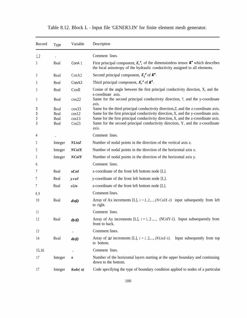
Table 8.12. Block L - Input file 'GENER3.IN' for finite element mesh generator.

Record Type Variable Description

1 ,23

_

Real

Comment lines.

ConA 1

3 Real

3 Real

3 Real

3 Real

RealRealRealReal

ConA2

ConA3

Cosll

cos22

cos33cos12cos13Cos23

4

5

5

5

6

7

7

7

8 , 9

10

_

Integer

Integer

Integer

First principal component, K,“, of the dimensionless tensor KA which describesthe local anisotropy of the hydraulic conductivity assigned to all elements.

Second principal component, KzA of KA.

Third principal component, K,* of K”.

Cosine of the angle between the first principal conductivity direction, X, and thex-coordinate axis.Same for the second principal conductivity direction, Y, and the y-coordinateaxis.Same for the third principal conductivity direction, Z, and the z-coordinate axis.Same for the first principal conductivity direction, X, and the y-coordinate axis.Same for the first principal conductivity direction, X, and the z-coordinate axis.Same for the second principal conductivity direction, Y, and the z-coordinateaxis.

Comment lines.

NLinZ

NColX

NColY

Number of nodal points in the direction of the vertical axis z.

Number of nodal points in the direction of the horizontal axis x.

Number of nodal points in the direction of the horizontal axis y.

Comment lines.

Real xCol

Real ycol

Real zLin

x-coordinate of the front left bottom node [L].

y-coordinate of the front left bottom node [L].

z-coordinate of the front left bottom node [L].

Comment lines.

Real dx(i)

11

12

Array of Ax increments [L], i = I, 2,..., (NColX-I). input subsequently from leftto right.

Comment lines.

Real dy(i)

13

14

Array of Ay increments [L], i = 1, 2 ,..., (NColY-1). Input subsequently fromfront to back.

Comment lines.

Real

_

dz(i)

15,16

17

_

n

Array of Az increments [L], i = 1, 2,..., (NLinZ-1). Input subsequently from topto bottom.

Comment lines.

Integer Number of the horizontal layers starting at the upper boundary and continuingdown to the bottom.

17 Integer Kode( n) Code specifying the type of boundary condition applied to nodes of a particular

100

Table 8.12. (continued)

Record Type Variable Description

17

17

17

17

17

17

17

17

Real hOld(n)

Real Conc(n)

Real Q(n)

Int

Real

Real

Real

Real

LayNum(n)

Beta(n)

Axz(n)

Bxz( n)

Dxz(n)

Initial value of the pressure head assigned to nodes of a particular horizontallayer n [L].

Initial value of the concentration assigned to nodes of a particular horizontallayer n [ML”].

Prescribed recharge/dischargerate assigned to node n, [L?‘]. Q(n) is negativewhen directed out of the system. When no value for Q(n) is needed, set Q(n)equal to zero.

Subregion number assigned to nodes of a particular horizontal layer n.

Value of the water uptake distribution, b(x,y,z), in the soil root zone assigned tonodes of a particular horizontal layer n [L”]. Set Beta(n) equal to zero ifhorizontal layer n lies entirely outside the root zone.

Nodal value of the dimensionless scaling factor IX,, associated with the pressurehead assigned to nodes of a particular horizontal layer n.

Nodal value of the dimensionless scaling factor CY~ associated with the saturatedhydraulic conductivity assigned to nodes of a particular horizontal layer n.

Nodal value of the dimensionless scaling factor (Y# associated with the watercontent assigned to nodes of a particular horizontal layer n.

In general, record 17 information is required for each horizontal layer n, startingwith n= 1 and continuing sequentially until n=NLinZ. Record 17 information forcertain horizontal layers may be skipped if several conditions are satisfied (seebeginning of this section).

101

8.2. Example Input Files

Table 8.13. Input data for example 1 (input file ‘SELECTOR.IN’).

*** BLOCK A: BASIC INFORMATION l ****************************************Heading'Example 1 - Column Test'LUnit TUnit MUnit (units are obligatory for all input data)'cm' 'sec' '-'MaxIt TolTh TolH (max. number of iterations and precis. tolerances)

20 .OOOl .lL W a t LChem CheckF ShortF FluxF AtmInF SeepF FreeD DrainFt f f t t f t f f

l ** BLOCK 8: MATERIAL INFORMATlON ***************************************NMat NLay hTabl hTabN NPar

1 1 .OOl 200. 9thr ths tha thm Alfa n KS Kk thk.02 -350 .02 .350 .0410 1.964 .000722 .000695 .2875

*** BLOCK C: TIME INFORMATION ********************************************dt dtMin dtMax DMul DMul2 MPL

1. -01 60. 1.1 .33 6TPrint(l),TPrint(2),...,TPrint(MPL)60 900 1800 2700 3600 5400

(print-time array)

*** BLOCK E: SEEPAGE INFORMATION (only if SeepF =.true.) ***************NSeep (number of seepage faces)

1NSP(l),NSP(2) ,.......,NSP(NSeep) (nunber of nodes in each s.f.)

4NP(i,l),NP(i,2),.....,NP(i,NSP(i)) (nodal number array of i-th s.f.)

221 222 223 224*** END OF INPUT FILE 'SELECTOR.IN ' ***************************************

102

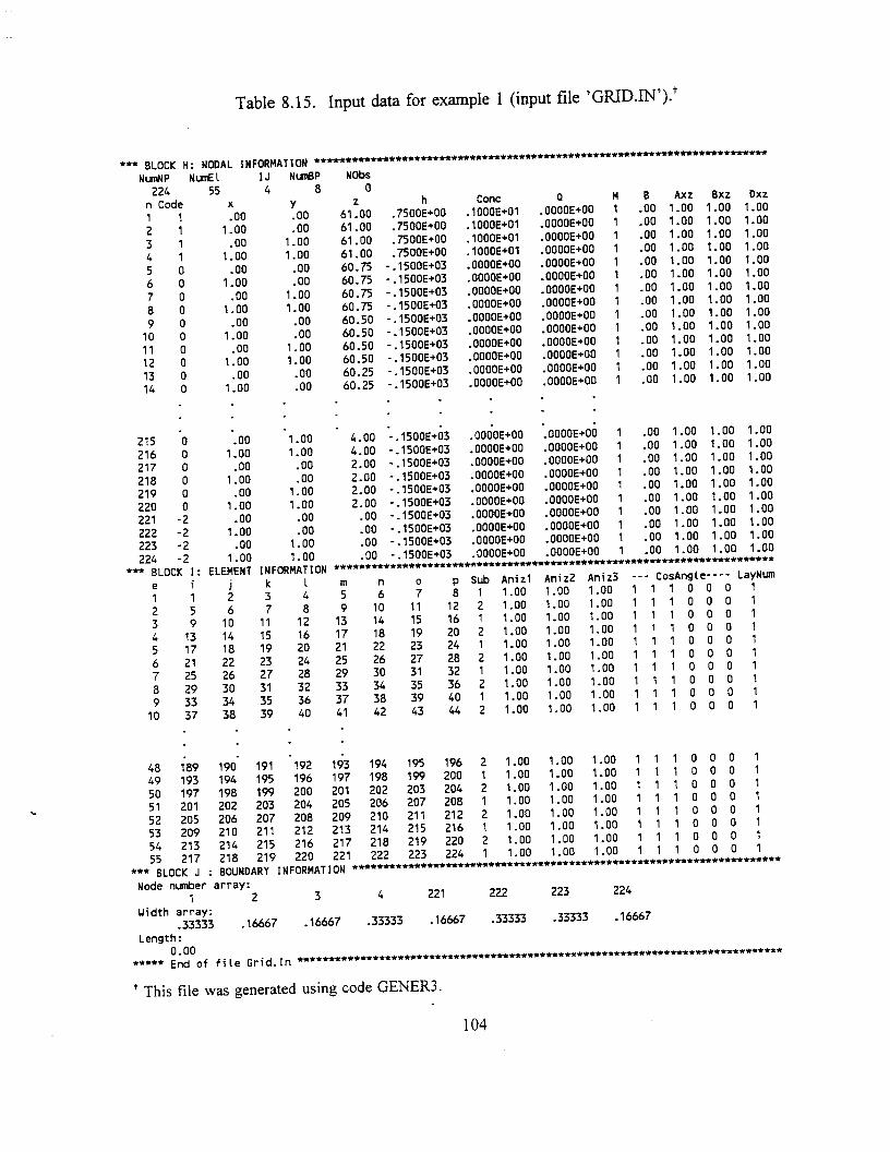
Table 8.16. Input data for example 2 (input file ‘SELECTOR.IN’).

*** BLOCK A: BASIC INFORMATION l ****************************************Heading'Example 2 - Grass Field Problem (Hupselse Beek 1982)'LUnit TUnit MUnit (indicated units are obligatory for all input data)'cm' 'day' '-'MaxIt TolTh TolH (max. number of iterations and precis. tolerances)

20 .OOOl 0.11Wat 1Chem CheckF ShortF FluxF AtmInF Seepf FreeD DrainF

f t*:* BLOCKfB: MATERIAL INFORMATION

t t f f f*~*****t*********f+**r*r**r*rr**r**+r*

NMat NLay hTabl hTabN NPar2 2 .OOl 1000. 9

thr ths tha thm Alfa n KS thk.OOOl .399 .OOOl .399 .0174 1.3757 29.75 ii.75 .399.OOOl .339 .OOOl .339 .0139 1.6024 45.34 45.34 .339*** BLOCK C: TIME INFORMATION t****~t******************~****************dt dtMin dtMax DMul DMul2 MPL.02 le-10 0.50 1.3 .3 6

TPrint(l),TPrint(2),...,TPrint(MPL) (print-time array)120 151 181 212 243 273

*** BLOCK D: SINK INFORMATION ***************************************PO P2H P2L P3 r2H r2L-10. -200. -800. -8000. 0.5 0.1

POptm(l),POptm(2),...,POptm(NMat)-25. -25.

l ** END OF INPUT FILE 'SELECTOR.IN ' ******************************

105

Table 8.17. Input data for example 2 (input fil e 'ATMOSPH.IN').

*** BLOCK K: ATMOSPHERIC INFORMATION **********************************

*** Hupselse Beek 1982 *****************************~*******CH******~****~**~*****~*~***~**~*~~**********~*****~***~*T*~~*~SinkF qGWLFt t

GWLOL Aqh Bqh (if qGWLF=f then Aqh=Bqh=O)230 -.1687 -.02674

tInit MaxAL (MaxALL = number of atmospheric data-records)90.

hCritS1e30tAtm

91929394

;:979899100

1 0 1102103104105106107108109110111112113114115116117118119120

183(max. allowed pressure head at the soil surface)

Prec cPrec rSoi1 rRoot hCritA rt ht crt cht0 0 0 0.16 1000000 0 0 0 0

0.07 0 0 0.18 1000000 0 0 0 00.02 0 0 0.13 1000000 0 0 0 0

0 0 0 0.20 1000000 0 0 0 00 0 0 0.28 1000000 0 0 0 0

0.07 0 0 0.18 1000000 0 0 0 00.29 0 0 0.08 1000000 0 0 0 00.44 0 0 0.14 1000000 0 0 0 00.20 0 0 0.11 1000000 0 0 0 00.29 0 0 0.11 1000000 0 0 0 00.32 0 0 0.11 1000000 0 0 0 00.49 0 0 0.11 1000000 0 0 0 00.01 0 0 0.16 1000000 0 0 0 0

0 0 0 0.17 1000000 0 0 0 00 0 0 0.22 1000000 0 0 0 00 0 0 0.21 1000000 0 0 0 00 0 0 0.23 1000000 0 0 0 00 0 0 0.23 1000000 0 0 0 00 0 0 0.24 1000000 0 0 0 00 0 0 0.18 1000000 0 0 0 00 0 0 0.15 1000000 0 0 0 00 0 0 0.19 1000000 0 0 0 0

0.01 0 0 0.15 1000000 0 0 0 00.01 0 0 0.22 1000000 0 0 0 0

0 0 0 0.23 1000000 0 0 0 00.02 0 0 0.20 1000000 0 0 0 0

0 0 0 0.17 1000000 0 0 0 00.02 0 0 0.14 1000000 0 0 0 00.26 0 0 0.13 1000000 0 0 0 00.24 0 0 0.11 1000000 0 0 0 0

256 0 - 0 - 0 '0.13 1000000257 0 0 0 0.14 1000000258 0 0 0 0.20 1000000259 0 0 0 0.14 1000000260 0 0 0 0.19 1000000261 0 0 0 0.14 1000000262 0 0263 0.35 0 :

0.20 10000000.23 1000000

264 0.52 0 0 0.16 1000000265 0 0 0 0.21 1000000266 0 0 0 0.19 1000000267 0 0 0 0.18 1000000268 0 0 0 0.18 1000000269 0.53 0 0 0.09 1000000270 0.07 0 0 0.23 1000000271 0 0 0 0.17 1000000272 0 0 0 0.22 1000000273 1.04 0 0

00000000000000000

0 1000000 0

000000000000000000

00000000000000000

00000000000000000

0 0*** END OF INPUT FILE 'ATMOSPH.IN ' t****t*****t*t********,**,t*************~*

106

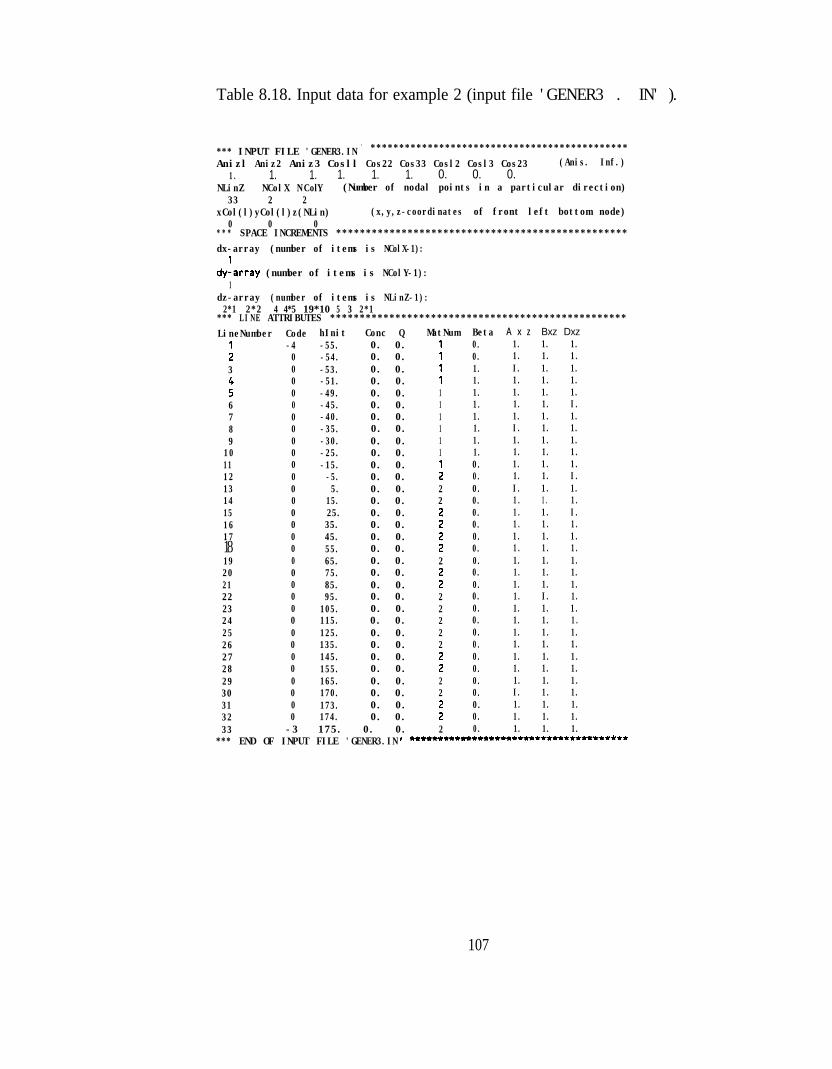
Table 8.18. Input data for example 2 (input file ' GENER3 . IN' ).

*** INPUT FILE 'GENER3.IN ' *********************************************Anizl Aniz2 Aniz3 Cosll Cos22 Cos33 Cosl2 Cosl3 Cos23 (Anis. Inf.)

1. 1. 1. 1. 1. 1. 0. 0. 0.NLinZ NColX NColY (Number of nodal points in a particular direction)

33 2 2xCol(l)yCol(l)z(NLin) (x,y,z-coordinates of front left bottom node)

0 0 0* * * SPACE INCREMENTS *************************************************dx-array (number of items is NColX-1):

dylarray (number of items is NColY-1):1

dz-array (number of items is NLinZ-1):2*1 2*22 4 4*5 19*100 5 3 2*1

*** LI N E ATTRIBUTES **************************************************LineNumber Code

:-40

3 0

;00

6 07 08 09 0

10 011 012 013 014 015 0 25.16 017 018 019 020 021 022 023 024 025 026 027 028 029 030 031 032 0

hInit-55.-54.-53.-51.-49.-45.-40.-35.-30.-25.-15.-5.5.

15.

35.45.55.65.75.85.95.

105.115.125.135.145.155.165.170.173.174.

Conc Q0. 0.0. 0.0. 0.0. 0.0. 0.0. 0.0. 0.0. 0.0. 0.0. 0.0. 0.0. 0.0. 0.0. 0.0. 0.0. 0.0. 0.0. 0.0. 0.0. 0.0. 0.0. 0.0. 0.0. 0.0. 0.0. 0.0. 0.0. 0.0. 0.0. 0.0. 0.0. 0.

MatNum

1

f111111

:22

:

:2

:22222

:22

:2

Beta0.0.1.1.1.1.1.1.1.1.0.0.0.0.0.0.0.0.0.0.0.0.0.0.0.0.0.0.0.0.0.0.0.

A x z Bxz Dxz1. 1. 1.1. 1. 1.I. 1. 1.1. 1. 1.1. 1. 1.1. 1. I.1. 1. 1.I. 1. 1.1. 1. 1.1. 1. 1.1. 1. 1.1. 1. I.I. 1. 1.1. 1 . 1.1. 1. I.1. 1. 1.1. 1. 1.1. 1. 1.1. 1. 1.1. 1. 1.1. 1. 1.1. I. 1.1. 1. 1.1. 1. 1.1. 1. 1.1. 1. 1.1. 1. 1.1. 1. 1.1. 1. 1.I. 1. 1.1. 1. 1.1. 1. 1.1. 1. 1.33 -3 175. 0. 0.

*** END OF INPUT FILE 'GENER3.IN ' *tt*******tt*+************************

107

Table 8.19. Input data for example 2 (input file ‘GRIDAN’).+

*** BLOCK H: NODAL INFORMATION *******************************************************************************NumNP NwnEl IJ NumBP NObs

132n Code1 -4

-4: -44 -45 06 07 08 09 010 011 012 013 014 015 016 017 018 019 020 0

32 4 8 0x Y.oo .oo

1.00 -00.00 1.00

1.00 1.00.00 .00

1.00 .00.00 1.00

1.00 1.00.00 .00

1.00 .00.0O 1.00

1.00 1.00.00 .00

1.00 .00.00 1.00

1.00 1.00.00 .00

1.00 .00.00 1.00

1.00 1.00.

127 0 . 0 0 '1.00128 0 1.00 1.00129 -3 .00 .00130 -3 1.00 .00131 -3 .00 1.00132 -3 1.00 1.00

h230fOO -.5500E+02230.00 -.5500E+O2230.00 -.550OE+02230.00 -.5500E+02229.00 -.5400E+02229.00 -.5400E+02229.00 -.5400E+02229.00 -.5400E+02228.00 -.5300E+02228.00 -.5300E+02228.00 -.5300E+02228.00 -.5300E+02226.00 -.5lOOE+02226.00 -.5lOOE+02226.00 -.5100E+02226.00 -.5100E+02224.00 -.4900E+02224.00 -.4900E+02224.00 -.4900E+02224.00 -.4900E+02

*1.00 .1740E+031.00 .1740E+03.00 .175OE+03.00 .175OE+03.O0 .175OE+03.00 .1750E+03

Conc Q M B Axz Bxz Dxz.OOOOE+OO .OOOOE+OO 1 .00 1.00 1.00 1.00.OOOOE+OO .OOOOE+OO 1 .00 1.00 1.00 1.00.OOOOE+OO .OOOOE+OO 1 .00 1.00 1.00 1.00.OOOOE+OO .OOOOE+OO 1 .00 1.00 1.00 1.00.OOOOE+OO .OOOOE+OO 1 .00 1.00 1.00 1.00.OOOOE+O0 .OOO0E+0O 1 .OO 1.00 1.00 1.00.OOOOE+OO .OOOOE+OO 1 .00 1.00 1.00 1.00.OOOOE+OO .OOOOE+OO 1 .00 1.00 1.00 1.00.OOOOE+OO .OOOOE+OO 1 1.00 1.00 1.00 1.00.OOOOE+OO .OOOOE+OO 1 1.00 1.00 1.00 1.00.OOOOE+OO .OOOOE+OO 1 1.00 1.00 1.00 1.00.OOOOE+OO .OOOOE+OO 1 1.00 1.00 1.00 1.00.OOOOE+OO .OOOOE+OO 1 1.00 1.00 1.00 1.00.OOOOE+0O .OOOOE+OO 1 1.00 1.00 1.00 1.00.OOOOE+OO .OO0OE+OO 1 1.00 1.00 1.00 1.00.OOOOE+OO .OOOOE+OO 1 1.00 1.00 1.00 1.00.OOOOE+OO .OOOOE+OO 1 1.00 1.00 1.00 1.00.OOOOE+OO .OOOOE+OO 1 1.00 1.00 1.00 1.00.OOOOE+OO .OOOOE+OO 1 1.00 1.00 1.00 1.00.OOOOE+OO .OOOOE+OO 1 1.00 1.00 1.00 1.00

.OOOOE+OO .OOOOE+00 2 .00 1.00 1.00 1.00

.000OE+OO .OO00E+O0 2 .OO 1.00 1.00 1.00

.OOOOE+OO .OOOOE+OO 2 .oo 1.00 1.00 1.00

.OOOOE+OO .OOOOE+OO 2 .oo 1.00 1.00 1.00

.OO0OE+OO .OO00E+OO 2 .OO 1.00 1.00 1.00

.OOOOE+OO .OOOOE+OO 2 .oo 1.00 1.00 1.00l ** BLOCK 1: ELEMENT INFORMATION **t**t****t*****t*****~************************************************

e i j k2 3

l m Sub Anizl Aniz2 Aniz3 --- CosAngle---- LayNum1 1 4 5 6" ; ! 1 1.00 1.00 1.00 1 1 1 0 0 0 12 5 6 7 8 9 10 11 12 2 1.00 1.00 1.00 1 1 1 0 0 0 13 9 10 11 12 13 14 1 1.00 1.00 1.00 1 1 1 0 0 0 14 13 14 15 16 17 18

15 1619 20 2 1.00 1.00 1.00 1 1 1 0 0 0 1

5 17 18 19 20 21 22 23 24 1 1.00 1.00 1.00 1 1 1 0 0 0 16 21 22 23 24 25 26 27 28 2 1.00 1.00 1.00 1 1 1 0 0 0 17 25 27 28 29 30 31 1 1.00 1.00 1.00 1 1 1 0 0 0 18 29 5: 31 32 33 34 35 if 2 1.00 1.00 1.00 1 1 1 0 0 0 19 33 34 35 36 37 38 39 40 1 1.00 1.00 1.00 1 1 1 0 0 0 1

10 37 38 39 40 41 42 43 44 2 1.00 1.00 1.00 1 1 1 0 0 0 1

25 9 7 98 99 100 l0l 102 103 104 1 1.00 1.00 1.00 1 1 1 0 0 0 226 101 102 103 104 105 106 107 108 2 1.00 1.00 1.00 1 1 1 0 0 0 227 105 106 107 108 109 110 111 112 1 1.00 1.00 1.00 1 1 1 0 0 0 228 109 110 111 112 113 114 115 116 2 1.00 1.00 1.00 1 1 1 0 0 0 229 113 114 115 116 117 118 119 120 1 1.00 1.00 1.00 1 1 1 0 0 0 230 117 118 119 120 121 122 123 124 2 1.00 1.00 1.00 1 1 1 0 0 0 231 121 122 123 124 125 126 127 128 1 1.00 1.00 1.00 1 1 1 0 0 0 232 125 126 127 128 129 130 131 132 2 1.00 1.00 1.00 1 1 1 0 0 0 2

*** BLOCK J : BOUNDARY INFORMATION t******t**************ttt**t*********************~*****~**.***************Node number array:

1 2 3 4 129 130 131 132Width array:

.33333 .16667 .16667 .33333 .16667 .33333 .33333 .16667Length:

1.00***** End of file Grid.In t**************tIrt********t*******

’ This file was generated with code GENER3.

108

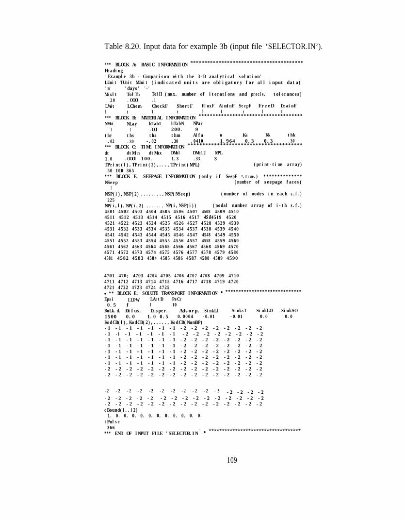
Table 8.20. Input data for example 3b (input file ‘SELECTOR.IN’).

*** BLOCK A: BASIC INFORMATION ****************************************Heading'Example 3b - Comparison with the 3-D analytical solution'LUnit TUnit MUnit (indicated units are obligatory for all input data)' m ' 'days' '-'Maxlt TolTh TolH (max. number of iterations and precis. tolerances)

20 .OOOl .1LWat LChem CheckF ShortF FluxF AtmInF SeepF FreeD DrainFf t f t f f t f f*** BLOCK B: MATERIAL INFORMATION *************************************NMat NLay hTab1 hTabN NPar

1 1 .OOl 200. 9thr ths tha thm Alfa n KS Kk thk.02 .30 -.02 .30 .0410 1.964 0.3 0.3 .30

*** BLOCK C: TIME INFORMATION ***************************************

dt dtMin dtMax DMul DMu12 MPL1.0 .OOOl 100. 1.3 .33 3TPrint(l),TPrint(2),...,TPrint(MPL) (print-time array)50 100 365

*** BLOCK E: SEEPAGE INFORMATION (only if SeepF =.true.) **************NSeep (number of seepage faces)

7NSP(l),NSP(2) ,.......,NSP(NSeep) (number of nodes in each s.f.)225

NP(i,l),NP(i,2) , . . . . . , NP(i,NSP(i)) (nodal number array of i-th s.f.)4501 4502 4503 4504 4505 4506 4507 4508 4509 45104511 4512 4513 4514 4515 4516 4517 45 8 4519 45204521 4522 4523 4524 4525 4526 4527 4528 4529 45304531 4532 4533 4534 4535 4534 4537 4538 4539 45404541 4542 4543 4544 4545 4546 4547 4548 4549 45504551 4552 4553 4554 4555 4556 4557 4558 4559 45604561 4562 4563 4564 4565 4566 4567 4568 4569 45704571 4572 4573 4574 4575 4576 4577 4578 4579 45804581 4582 4583 4584 4585 4586 4587 4588 4589 4590

4701 470; 4703 4704 4705 4706 4707 4708 4709 47104711 4712 4713 4714 4715 4716 4717 4718 4719 47204721 4722 4723 4724 4725l ** BLOCK E: SOLUTE TRANSPORT INFORMATION l *****************************Epsi LUPW LArtD PeCr0.5 f f 10

BuLk.d. Difus. Disper. Adsorp. SinkLl Sinks1 SinkLO SinkSO1500 0.0 1.0 0.5 0.0004 -0.01 -0.01 0.0 0.0KodCB(l),KodCB(2),.....,KodCB(NumBP)-1 -1 -1 -1 -1 -1 -1 -2 -2 -2 -2 -2 -2 -2 -2-1 -1 -1 -1 -1 -1 -1 -2 -2 -2 -2 -2 -2 -2 -2-1 -1 -1 -1 -1 -1 -1 -2 -2 -2 -2 -2 -2 -2 -2-1 -1 -1 -1 -1 -1 -1 -2 -2 -2 -2 -2 -2 -2 -2-1 -1 -1 -1 -1 -1 -1 -2 -2 -2 -2 -2 -2 -2 -2-1 -1 -1 -1 -1 -1 -1 -2 -2 -2 -2 -2 -2 -2 -2-1 -1 -1 -1 -1 -1 -1 -2 -2 -2 -2 -2 -2 -2 -2-2 -2 -2 -2 -2 -2 -2 -2 -2 -2 -2 -2 -2 -2 -2-2 -2 -2 -2 -2 -2 -2 -2 -2 -2 -2 -2 -2 -2 -2

-2 -2 -2 -2 -2 -2 -2 -2 -2 -2 - 2 -2 -2 -2 -2-2 -2 -2 -2 -2 -2 -2 -2 -2 -2 -2 -2 -2 -2 -2-2 -2 -2 -2 -2 -2 -2 -2 -2 -2 -2 -2 -2 -2 -2cBound(l..l2)1. 0. 0. 0. 0. 0. 0. 0. 0. 0. 0. 0.

tPulse366

*** END OF INPUT FILE 'SELECTOR.IN ' l ***********************************

109

Table 8.22. Input data for example 3 (input file ‘GRID.IN’).+

*** BLOCK H: NODAL INFORMATION **************************************************************************

N u m N P N u m E l IJ NumBP NObs4725 3920 225 450 0n Code X Y z h Conc Q M B Axz Bxz Dxz1 1 .oo .OO .oo .OOOOE+OO .OOOOE+OO .OOOOE+OO 1 .oo 1.00 1.00 1.002 1 10.00 .oo .oo .OOOOE+OO .OOOOE+OO .OOOOE+OO 1 -00 1.00 1.00 1.003 1 20.00 .oo .oo .OOOOE+OO .OOOOE+oO .OOOOE+OO 1 .oo 1.00 1.00 1.004 1 30.00 .oo .OO .OOOOE+OO .OOOOE+OO .OOOOE+OO 1 .oo 1.00 1.00 1.005 1 40.00 .OO .oo .OOOOE+OO .OOOOE+OO .OOOOE+OO 1 .00 1.00 1.00 1.006 1 45.00 .oo .oo .OOOOE+Oo .OOOOE+OO .OOOOE+OO 1 .oo 1.00 1.00 1.007 1 49.00 .oo .oo .OOOOE+OO .OOOOE+OO .OOOOE+OO 1 .oo 1.00 1.00 1.008 1 51.00 .OO .oo .OOOOE+00 .OOOOE+OO .OOOOE+OO 1 -00 1.00 1.00 1.009 1 55.00 -00 .oo .OOOOE+OO .OOOOE+OO .OOOOE+OO 1 .oo 1.00 1.00 1.00

.. . .

4720 '2 6O:OO 120.00 -200.00 *.OOOOE+OO .O00OE+OO OOOOE+O0 1 .oo 1.00 1.00 1.004721 2 67.00 120.00 -200.00 .OOOOE+OO .OOOOE+OO .OOOOE+OO 1 .oo 1.00 1.00 1.0047224723 f

75.00 120.00 -200.00 .OOOOE+OO .OOOOE+OO .OOOOE+OO 1 .oo 1.00 1.00 1.0085.00 120.00 -200.00 .OO0OE+00 .OOOOE+OO .OOOOE+OO 1 .oo 1.00 1.00 1.00

4724 2 100.00 120.00 -200.00 .OOOOE+OO .OOOOE+OO .OOOOE+OO 1 .oo 1.00 1.00 1.004725 2 120.00 120.00 -200.00 .OOOOE+OO .OOOOE+OO .OOOOE+OO 1 .oo 1.00 1.00 1.00

*** BLOCK 1: ELEMENT INFORMATION ************************************.**********************************e. . k L1 ; : 16 17 22: 22; 24;) 24;

Sub Anizl Aniz2 Aniz3 --- CosAngle --- LayNum1 1.00 1.00 1.00 1 1 1 0 0 0 1

2 2 3 17 18 227 228 242 243 2 1.00 1.00 1.00 1 1 1 0 0 0 13 3 4 18 19 228 229 243 244 1 1.00 1.00 1.00 1 1 1 0 0 0 14 4 5 19 20 229 230 244 245 2 1.00 1.00 1.00 1 1 1 0 0 0 15 5 6 20 21 230 231 245 246 1 1.00 1.00 1.00 1 1 1 0 0 0 16 6 7 21 22 231 232 246 247 2 1.00 1.00 1.00 1 1 1 0 0 0 17 7 8 22 23 232 233 247 248 1 1.00 1.00 1.00 1 1 1 0 0 0 1

3917 4481 4482' 4496 4497 4766 4707 4721 4722 1 1.00 1.00 1.00 1 1 1 0 0 0 13918 4482 4483 4497 4498 4707 4708 4722 4723 2 1.00 1.00 1.00 1 1 1 0 0 0 13919 4483 4484 4498 4499 4708 4709 4723 4724 1 1.00 1.00 1.00 1 1 1 0 0 0 13920 4484 4485 4499 4500 4709 4710 4724 4725 2 1.00 1.00 1.00 1 1 1 0 0 0 1

*** BLOCK J : B O U N D A R Y I N F O R M A T I O N tt*‘tt*ll**rCll**tlt*******t**************Node number array:

1 2 3 49 10 11 12

4662 4'693 '4694 46954700 4701 4702 47034708 4709 4710 471147164724

Width array:33.3333330.00000

75. 0 0 0 0 087.50000

145.8333030.00000116.66670

Length:0.00

47174725

4718 4719

4696' 4697 4 6 9 8 46994704 4705 4706 47074712 4713 4714 47154720 4721 4722 4723

33.33333 66.66666 33.33333 50.00000 15.00000 20.00000 10.0000020.00000 50.00000 30.00000 83.33334 58.33333 66.66666 33.33333

208.33330 145.83330105.00000 35.00000408.33330 116.6667040.00000 20.00000133.33330

166.66670 58.33333 233.33330 116.66670 233.3333070.00000 52.50000 140.00000 87.50000 210.0000066.66666 66.66666 133.33330 66.66666 100.0000060.00000 40.00000 100.00000 60.00000 166.66670

5 6 7 a13 14 15 16

l **** End of file Grid.In **********************************************************************************

’ This file was generated using code GENER3.

111

Table 8.23. Input data for example 4 (input file ‘SELECTORIN’).

*** BLOCK A: BASIC INFORMATION *************************************Heading'Example 4 - Contaminant Transport from a Waste Disposal Site'LUnit TUnit MUnit BUnit (units are obligatory for all input data)'m' 'day' '-' '-'

MaxIt TolTh To l H (maximun number of iterations and tolerances)20 .OOOl 0.01

L W a t LChem ChecF ShortF FluxF AtmInF SeepF FreeD DrainFf t tl :* gLOCKtg: MATERIAL INFORMATION

f t f f**.ftlrCN**~****t*~****************-

NMat NLay hTab1 hTabN NPar1 1 .OOl 200. 9

thr ths tha thm Alfa KS Kk thk.05 .45 .05 .45 4.1 z.0 5.0 5.0 .4500

l ** BLOCK C: TIME INFORMATION l *************.***********~**********~**dt dtMin dtMax DMUl DMul2 MPL0.001 .OOOl 0.1 1.1 .33 9

TPrint(l),TPrint(2),...,TPrint(MPL) (print-time array)0.25 1.5 5 10 20 30 50 100 200

l ** BLOCK E: SEEPAGE INFORMATION (only if SeepF =.true.) *************NSeep (number of seepage faces)

1NSP(l),NSP(2) ,.......,NSP(NSeep) (number of nodes in each s.f.)

7NP(i,l),NP(i,2) , . . . . . , NP(i,NSP(i)) (nodal number array of i-th s.f.)3191 3719 4247 4775 5303 5831 6359

*** BLOCK G: SOLUTE TRANSPORT INFORMATION* * * * * * * * * * * * * * * * * * * * * * *Epsi LUPW LArtD PeCr0.5 f t 2.

Bu1k.d. Difus. Disper. Adsorp. SinkLl Sinks1 SinkLO SinkSO1.400 0.01 1.0 0.25 0.0 0.0 0.0 0.0 0.0KodCB(l),KodCE(2),.....,KodCB(NunBP)54*-1 577*-2cBound(l..l2)1. 0. 0. 0. 0. 0. 0. 0. 0. 0. 0. 0.tPulse50

l ** END OF INPUT FILE 'SELECTOR.IN , ******************************

112

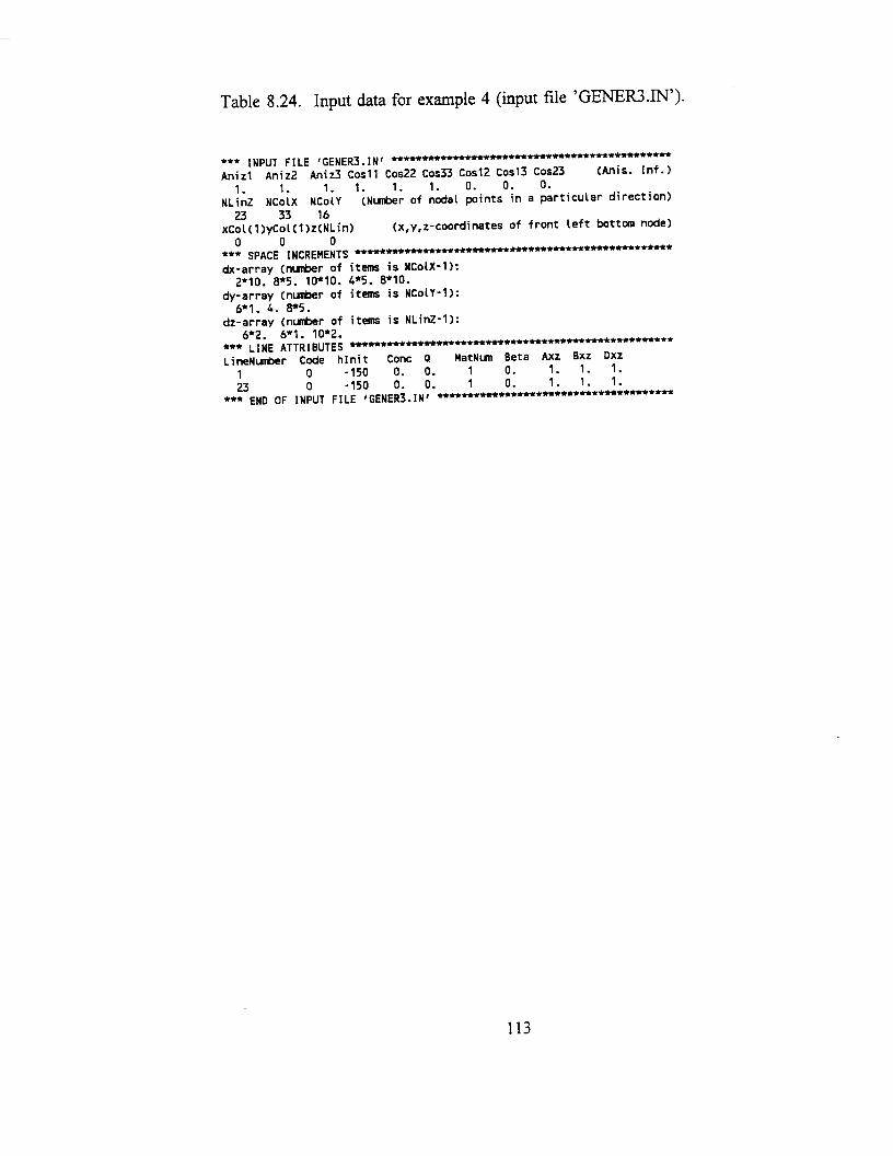
Table 8.25. Input data for example 4 (input file ‘GRID.IN’).+

*** BLOCK H: NODAL INFORMATION +*Cl*mTt****~*H*t********~****t~~*NumNP NumEl NumBP NObs12144 10560 631 4n Code X Y z h Conc Q M B Axz Bxr Dxz123456789

::121314151617

0 .00 100 38.00 -.lOOOE+O2 .OOOOE+OO .OOOOE+OO 1 .oo 1.00 1.00 1.000 10.00 .oo 38.00 -.1008E+02 .OOOOE+OO .OOOOE+OO 1 -00 1.00 1.00 1.001 20.00 .oo 38.00 .OOOOE+OO .OOOOE+OO .OOOOE+OO 1 -00 1.00 1.00 1.001 25.00 .OO 38.00 .OOOOE+OO .0000E+00 .OOOOE+OO 1 .00 1.00 1.00 1.001 30.00 .oo 38.00 .OOOOE+OO .OOOOE+OO .0000E+00 1 .00 1.00 1.00 1.001 35.00 .00 38.00 .OOO0E+OO .OOOOE+OO .OOOOE+OO 1 .00 1.00 1.00 1.001 40.00 .oo 38.00 .OOOOE+OO .OOOOE+OO .OOOOE+OO 1 .oo 1.00 1.00 1.001 45.00 .oo 38.00 .OOOOE+OO .OOOOE+OO .OOOOE+OO 1 .oo 1.00 1.00 1.001 50.00 .oo 38.00 .OOOOE+OO .OOOOE+OO .OOOOE+OO 1 -00 1.00 1.00 1.001 55.00 .oo 38.00 .0000E+00 .OOOOE+OO .OOOOE+OO 1 -00 1.00 1.00 1.001 60.00 .00 38.00 .OOOOE+OO .OOOOE+OO .OOOOE+OO 1 -00 1.00 1.00 1.000 70.00 .DO 38.00 -.1054E+02 .OOOOE+OO .OO0OE+OO 1 -00 1.00 1.00 1.000 80.00 .oo 38.00 -.1062E+02 .OOOOE+OO .OOOOE+OO 1 .00 1.00 1.00 1.000 90.00 .oo 38.00 -.1069E+02 .OOOOE+OO .OOOOE+OO 1 .oo 1.00 1.00 1.000 100.00 .00 38.00 -.1077E+02 .OOOOE+OO .OOOOE+OO 1 .oo 1.00 1.00 1.000 110.00 .oo 38.00 -.1085E+02 .OOOOE+OO .OOOOE+OO 1 .00 1.00 1.00 1.000 120.00 .oo 38.00 -.1092E+02 .OOOOE+OO .OOOOE+OO 1 .00 1.00 1.00 1.00

12141121421214312144

0 230.00 50.00 .oo .2623E+02 .OOOOE+OO0 240.00 50.00 .oo .2615E+02 .OOOOE+OO0 250.00 50.00 .oo .2608E+02 .OOOOE+OO

.OOOOE+O0

.OOOOE+OO

.OOOOE+OO

1 .00 1.00' 1.00 1.001 .oo 1.00 1.00 1.001 .oo 1.00 1.00 1.00

1 260.00 50.00 .00 .2600E+02 .OOOOE+OO .OOOOE+OO 1 -00 1.00 1.00 1.00*** BLOCK I: ELEMENT INFORMATION ***********************************************************************e. k p Sub Anizl Aniz2 Aniz3 ------ CosAngle ------- Lay1 ; : 34 3: 52: 53: 56; 563 1 1.00 1.00 1.00 1.0 1.0 1.0 .o .o .o 12 2 3 35 36 530 531 563 564 2 1.00 1.00 1.00 1.0 1.0 1.0 .o .o .o 13 3 4 36 37 531 532 564 565 i 1.00 1.00 1.00 1.0 1.0 1.0 .o .o .o- 14 4 5 :5 38 532 533 565 566 2 1.00 1.00 1.00 1.0 1.0 1.0 .o .o .o 15 5 6 39 533 534 566 567 1 1.00 1.00 1.00 1.0 1.0 1.0 .O .O .O 1

. .

10558 11580 11581 11613 11614 12108.

12109 12141 12142 1 -1.00 1.00 1.00' 1.0 1.0 1.0 . 0 .o .o 110559 11581 11582 11614 11615 12109 12110 12142 12143 2 1.00 1.00 1.00 1.0 1.0 1.0 .0 .o .o 110560 11582 11583 11615 11616 12110 12111 12143 12144 1 1.00 1.00 1.00 1.0 1.0 1.0 .o .0 .o 1l ** BLOCK J : BOUNDARY INFORMATION *2*.t******.t***t******.******************.******.****.**********.***Node number array:

3 4 53:

7 8 9 1011 36 37 39 40 4243 44 69 70 71 72 74

. .

l-1913 11911 - - 11980 -11946 11947 11979 12012 1201312045 12046 12078 12079 12111 12112 12144

Uidth array:5.000005.000006.66667

1.66667 3.33333 .83333 3.33333 1.66667 3.33333 1.666675.00000 6.66667 3.33333 3.33333 3.33333 6.66667 3.333335.00000 10.00000 3.33333 6.66667 1.66667 6.66667 3.33333

6.66667 3.3333; -3.33333 6.66667 d.66667 3.33333 -3.33333 6.666676.66667 3.33333 3.33333 6.66667 6.66667 1.66667 1.66667

Length:.00

Observation nodes1591 4244 6363 6887

l **** End of file Grid.In t*****t***t******t*~****+t*****

’ This file was generated using code GENER3 with subsequent editing of boundary conditions.

114

9. OUTPUT DATA

The program output consists of 17 output files organized into 3 groups:

T-level informationH_MEAN.OUTV_MEAN.OUTCUMQ.OUTRUN_INF.OUTSOLUTE.OUTOBSNOD.OUT

P-level informationH.OUTTH.OUTCONC.OUTQ.OUTVX.OUTVY.OUTVZ.OUTBOUNDARY.OUTBALANCE.OUT

A-level informationA_LEVEL.OUT

In addition, some of the input data are printed to file CHECKOUT. All output files are

directed to subdirectory SWMS_3D.OUT, which must be created by the user prior to program

execution. The various output files are described in detail in Section 9.1. Section 9.2 lists

selected output files for examples 1 through 3 (see Section 7). The input files for these examples

were discussed in Section 8.2.

9.1. Description of Data Output Files

The file CHECKOUT contains a complete description of the finite element mesh, the

boundary code of each node, and the hydraulic and transport properties of each soil material.

Finite element mesh data are printed only when the logical variable CheckF in input Block A

115

(Table 9.1) is set equal to .true..

T-level information - This group of output files contains information which is printed at

the end of each time step. Printing can be suppressed by setting the logical variable ShortF in

input Block A equal to true.; the information is then printed only at selected print times. Output

files printed at the T-level are described in Tables 9.1 through 9.5. Output file OBSNOD.OUT

contains information about the transient changes in pressure head, water content, and solute

concentration at specified observation nodes.

P-level information - P-level information is printed only at prescribed print times. The

following output files are printed at the P-level:

H.OUT

TH.OUT

CONC.OUT

Q.OUT

VX.OUT

VY.OUT

VZ.OUT

BOUNDARY.OUT

BALANCE.OUT

Nodal values of the pressure head

Nodal values of the water content

Nodal values of the concentration

Discharge/recharge rates assigned to boundary or internal sink/ sourcenodes

Nodal vaiues of the x-components of the Darcian flux vector

Nodal values of the y-components of the Darcian flux vector

Nodal values of the z-components of the Darcian flux vector

This file contains information about each boundary node, n, for whichKode(n) r 0, including the discharge/recharge rate, Q(n), the boundaryflux, q(n), the pressure head h(n), the water content 0(n), and theconcentration Conc(n).

This file gives the total amount of water and solute inside each specifiedsubregion, the inflow/outflow rates to/from that subregion, together withthe mean pressure head (hMean) and the mean concentration (cMean)over each subregion (see Table 9.6). Absolute and relative errors in thewater and solute mass balances are also printed to this file.

The output files H.OUT, TH.OUT, CONC.OUT, Q.OUT, VX.OUT, VY.OUT and

VZ.OUT provide printed tables of the specific variables. To better identify the output, each

printed line starts with the nodal number

which information is printed. Users can

the output for their specific needs.

and spatial coordinates of the first node on that line for

easily reprogram the original subroutines to restructure

116

A-level information - A-level information is printed each time a time-dependent boundary

condition is specified. The information is directed to output file A_LEVEL.OUT (Table 9.7).

117

Table 9.1. H_MEAN.OUT - mean pressure heads.

hAtm Mean value of the pressure head calculated over a set of nodes for which Kode(n)=f4 (i.e., along partof a boundary controlled by atmospheric conditions) [L].

hRoot

hKode3

Mean value of the pressure head over a region for which Beta(n)>0 (i.e., within the root zone) [L].

Mean value of the pressure head calculatedover a set of nodes for which Kode(n)=+3 (i.e., along partof a boundary where the groundwater level, the bottom flux, or other time-dependent pressure headand/or flux is imposed) [L].

hKode 1 Mean value of the pressure head calculatedover a set of nodes for which Kode(n)=+l (i.e., along partof a boundary where time-independent pressure heads and/or fluxes are imposed) [L].

hSeep

hKode5

Mean value of the pressure head calculated over a set of nodes for which Kode(n)=G (i.e., alongseepage faces) [L].

Mean value of the pressure head calculated over a set of nodes for which Kode(n)=+5 [L].

hKodeN Mean value of the pressure head calculated over a set of nodes for which Kode(n)=INumKD [L].

118

Table 9.2. V_MEAN.OUT - mean and total water fluxes.+

rAtm

rRoot

vAtm

vRoot

vKode3

vKode 1

vSeep

vKode5

vKodeN

Potential surface flux per unit atmospheric boundary (Kode(n)=k4) [LT’].

Potential transpiration rate, TP [LT’].

Mean value of actual surface flux per unit atmospheric boundary (Kode(n)=+4) [LT’].

Actual transpiration rate, T, [LT’].

Total value of the bottom or other flux across part of a boundary where the groundwater level, thebottom flux, or other time-dependent pressure head and/or flux is imposed (Ko&(n)+3) [L’T’].

Total value of the boundary flux accros part of a boundary where time-independent pressure headsand/or fluxes are imposed, including internal sinks/sources (Kode(n)=+l) [LIT’].

Total value of the boundary flux across a potential seepage face (Kode(n)=S) [L3T’].

Total value of the flux across a boundary containing nodes for which Kode(n)=+5 [L’T’].

Total value of the flux across a boundary containing nodes for which Kode(n)=flumKLI fL3T’].

+ Boundary fluxes are positive when water is removed from the system.

119

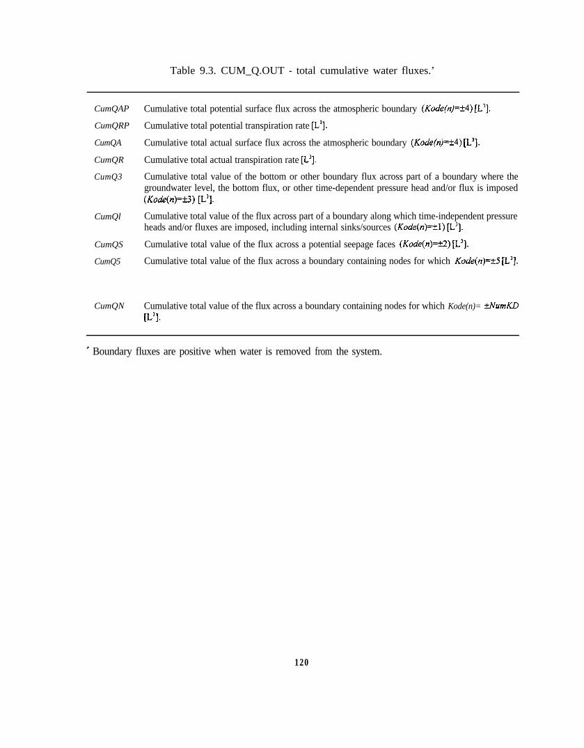
Table 9.3. CUM_Q.OUT - total cumulative water fluxes.’

CumQAP Cumulative total potential surface flux across the atmospheric boundary (Kode(n)=+4) [L’].

CumQRP Cumulative total potential transpiration rate [L’].

CumQA Cumulative total actual surface flux across the atmospheric boundary (Kode(n)=+4) [L3].

CumQR Cumulative total actual transpiration rate [L3].

CumQ3 Cumulative total value of the bottom or other boundary flux across part of a boundary where thegroundwater level, the bottom flux, or other time-dependent pressure head and/or flux is imposed(Kode(n)=ti) [L3].

CumQl Cumulative total value of the flux across part of a boundary along which time-independent pressureheads and/or fluxes are imposed, including internal sinks/sources (Kode(n)=+-1) [L3].

CumQS Cumulative total value of the flux across a potential seepage faces (Kode(n)=k2) [L’].

CumQ5 Cumulative total value of the flux across a boundary containing nodes for which Kode(n)=+5 [L3].

CumQN Cumulative total value of the flux across a boundary containing nodes for which Kode(n)= kNumKD[L31.

’ Boundary fluxes are positive when water is removed from the system.

120

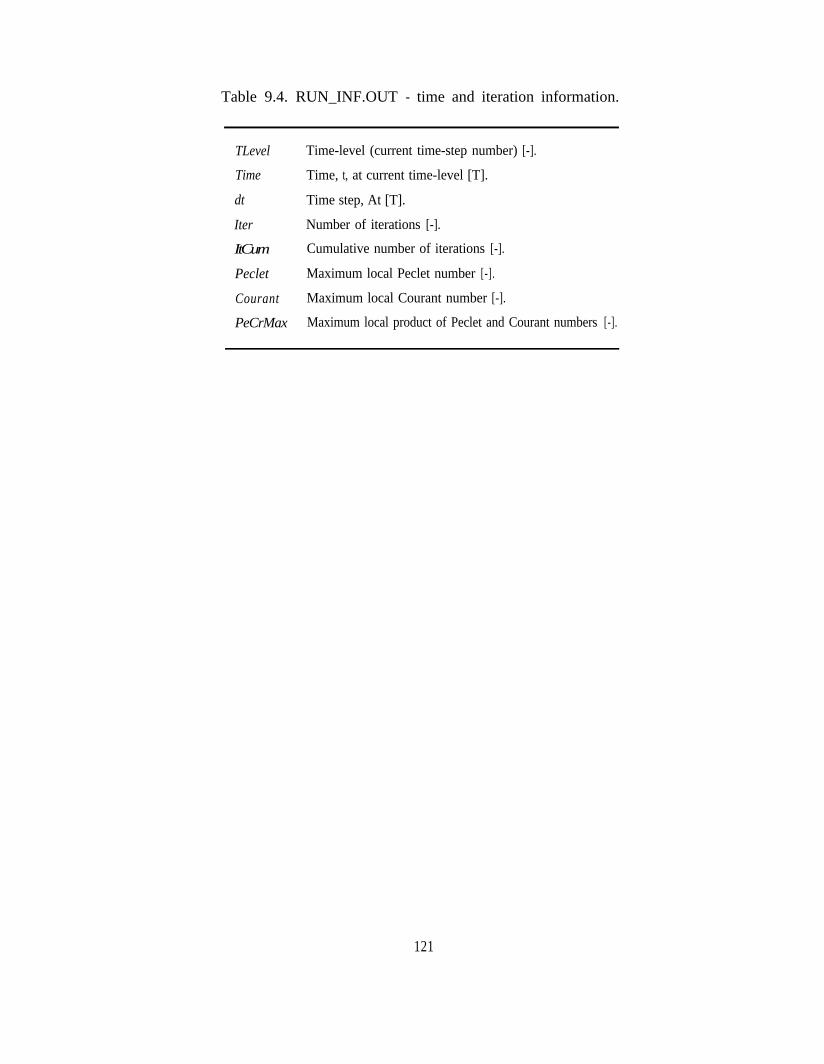
Table 9.4. RUN_INF.OUT - time and iteration information.

TLevel

Time

dt

Iter

ItCum

Peclet

Courant

PeCrMax

Time-level (current time-step number) [-].

Time, t, at current time-level [T].

Time step, At [T].

Number of iterations [-].

Cumulative number of iterations [-].

Maximum local Peclet number [-].

Maximum local Courant number [-].

Maximum local product of Peclet and Courant numbers [-].

121

Table 9.5. SOLUTE.OUT - actual and cumulative concentration fluxes.

CumCh0

CumCh 1

CumChR

ChemS1

ChemS2

ChemS3

ChemS4

ChemS5

ChemSN

qc1

qc2

qc3

qc4

qc5

qcN

Cumulative amount of solute removed from the flow region by zero-order reactions (positive whenremoved from the system) [M].

Cumulative amount of solute removed from the flow region by first-order reactions [M].

Cumulative amount of solute removed from the flow region by root water uptake S [M].

Cumulative solute flux across part of a boundary along which time-independent pressure heads and/orfluxes are imposed, including internal sink/sources (Kode(n)=fl) [M].

Cumulative solute flux across a potential seepage faces (Kode(n)=ti) [M].

Cumulative solute flux across part of a boundary along which the groundwater level, the bottom flux,or other time-dependent pressure head and/or flux is imposed (Kode(n)=+3) [M].

Cumulative total solute flux across the atmospheric boundary (Kode(n)=-+4) [M].

Cumulative total solute flux across an internal or external boundary containing nodes for whichK&e(n)=+5 [M].

Cumulative total solute flux across an internal or external boundary containing nodes for whichKode(n)=-+-NumKLl [M].

Total solute flux across part of a boundary along which time-independent pressure heads and/or fluxesare imposed (Kode(n)=fl) [MT’].

Total solute flux across a potential seepage face (Kode(n)=tZ) [MT’].

Total solute flux calculatedacross a boundary containing nodes for which Kode(n)=+_3 (i.e., along partof a boundary where the groundwater level, the bottom flux, or other tune-dependent pressure headand/or flux is specified) [MT’].

Total solute flux across the atmospheric boundary (Kode(n)=k4) [MT’].

Total solute flux across an internal or external boundary containing nodes for which Kode(n)= +5{MT-‘].

Total solute flux across an internal or external boundary containing nodes for which Kode(n)=HumKD [MT’].

122

Table 9.6. BALANCE.OUT - mass balance variables.

Area

Volume

InFlow

hMean

Conc Vol

cMean

WatBalT

WatBalR

CncBalT

CncBalR

Volume of the entire flow domain or a specified subregion [L3].

Volume of water in the entire flow domain or a specified subregion [L’].

Inflow/Outflow to/from the entire flow domain or a specified subregion [L’T’].

Mean pressure head in the entire flow domain or a specified subregion [L].

Amount of solute in the entire flow domain or a specified subregion [M].

Mean concentration in the entire flow domain or a specified subregion [MLJ].

Absolute error in the water mass balance of the entire flow domain [L’].

Relative error in the water mass balance of the entire flow domain [%].

Absolute error in the solute mass balance of the entire flow domain [M].

Relative error in the solute mass balance of the entire flow domain [%].

123

Table 9.7. A_LEVEL.OUT - mean pressure heads and total cumulative fluxes.+

CumQAP

CumQRP

CumQA

CumQR

CumQ3

hAtm

hRoot

hKode3

Cumulative total potential flux across the atmospheric boundary (Kode(n)=+4) [L’].

Cumulative total potential transpiration rate [L’].

Cumulative total actual flux across the atmospheric boundary (Kou’e(n)=+4) [L’].

Cumulative total actual transpiration rate [L’].

Cumulative total bottom or other flux across a boundary along which the groundwater level, thebottom flux, or other time-dependent pressure head and/or flux is imposed (Kode(n)=ti) [L3].

Mean value of the pressure head calculated over a set of nodes for which Kode(n)=k4 [L].

Mean value of the pressure head over a region for which Beta(n)>0 (i.e., the root zone) [L].

Mean value of the pressure head over a set of nodes for which Kode(n)=+_3 [L].

t Boundary fluxes are positive when water is removed from the system.

124

9.2. Example Output Files

Table 9.8. Output data for example 1 (part of output file ‘H.OUT’).

lime *** 5400.0000 l **

n x(n) Y(n) z(n) h(n) h(n+l) . . .

159

13172125293337414549535761656973778185899397

101105109113117121125129133137141145149153157161165169173177181185189193197201205209213217

.O

.O

.O

.O

.O

.O

.O

.O

.O

.O

.O

.O

.O

.O

.O

.O

.O

.O

::

::-0.O.O.O.O.O.O.O.O.O.O .0.O.O.O.O.O.O.O.O.O.O.O.O.O.O.O.O.O.O.O.O.O.O.O

.O

.O

.O

.O

.O

.O

.O

.O

.O

.O

.O

.O

.O

.O

.O

.O

.O

.O

.O

.O

.O

.O

.O

.O

.O

.O

.O

.O

.O

.O

.O

.O

.0

.O

.O

.O

.O

.O

.O

.O

.O

.O

.O

.O

.O

.O

.O

.O

.O

.O

.O

.O

.O

.O

.O

61.060.860.560.360.059.559.058.057.056.055.054.053.052.051.050.049.048.047.046.045.044.043.042.047.040.039.038.037.036.035.034.033.032.031.030.029.028.027.026.025.024.023.022.021.020.018.016.014.012.010.08.06.04.02.0.O

.8

.6

.4

.3

.l-.2-.5

-1.2-1.8-2.4-3.1-3.7-4.4-5.0-5.7-6.3-7.0-7.6-8.2-8.9-9.5

-10.1-10.7-11.4-12.0-12.6-13.1-13.7-14.3-14.9-15.4-15.9-16.5-17.0-17.5-18.1-18.8-19.5-20.3-21.3-22.4-23.8-25.5-27.8-30.7-34.9-48.5-81.8

-137.1-149.4-150.0-150.0-149.9-149.7-149.0-147.4

.8

.6

:i

-::-.5

-1.2-1.8-2.4-3.1-3.7-4.4-5.0-5.7-6.3-7.0-7.6-8.2-8.9-9.5

-10.1-10.7-11.4-12.0-12.6-13.1-13.7-14.3-14.9-15.4-15.9-16.5-17.0-17.5-18.1-18.8-19.5-20.3-21.2-22.4-23.8-25.6-27.7-30.8-34.7-49.0-87.5

-136.5-149.6-150.0-150.0-149.9-149.7-149.0-147.5

:34.l

-.2-.5

-1.2-1.8-2.4-3.1-3.7-4.4-5.0-5.7-6.3-7.0-7.6-8.2-8.9-9.5

-10.1-10.7-11.4-12.0-12.6-13.1-13.7-14.3-14.9-15.4-15.9-16.5-17.0-17.5-18.1-18.8-19.5-20.3-21.2-22.4-23.8-25.6-27.7-30.8-34.7-49.0-81.5

-136.5-149.6-150.0-150.0-149.9-149.7-149.0-147.5

:68:i.l

-.2-.5

-1.2-1.8-2.4-3.1-3.7-4.4-5.0-5.7-6.3-7.0-7.6-8.2-8.9-9.5

-10.1-10.7-11.4-12.0-12.6-13.1-13.7-14.3-14.9-15.4-15.9-16.5-17.0-17.5-18.1-18.8-19.5-20.3-21.3-22.4-23.8-25.5-27.8-30.7-34.9-48.5-81.8

-137.1-149.4-150.0-150.0-149.9-149.7-149.0

221 -147.4

125

Table 9.9. Output data for example 1 (output file ‘CUM_Q.OUT’).

Example I - Colum Test

Program SWMS_3DDate: 16. 8. Time: 9:24: 9Time independent boundary conditionsUnits: L = cm , T = sec , M = -All cumulative fluxes (CumQ) are positive out of the region

Time CumQAP CumQRP CumQA CumQR CumQ3 CumQ1[T] [V] [V] [V] [V] [V] [V]

60.0000 .OOOE+OO .OOOE+OO .OOOE+OO .OOOE+OO .O0OE+OO -.801E+OO900.0000 .OOOE+OO .OOOE+OO .OOOE+OO .OOOE+OO .OOOE+OO -.340E+O11800.0000 .OOOE+OO .OOOE+OO .OOOE+OO .OOOE+OO .OOOE+OO -.506E+Ol2700.0000 .OOOE+OO .OOOE+OO .OOOE+OO .OOOE+OO .OOOE+OO -.644E+O13600.0000 .OOOE+OO .OOOE+OO .OOOE+OO .OOOE+OO .OOOE+OO -.768E+O15400.0000 .OOOE+OO .OOOE+OO .OOOE+O0 .OOOE+OO .OOOE+OO -.991E+O1

CumQS[V]

.OOOE+OO

.OOOE+OO

.OOOE+OO

.OOOE+OO

.OOOE+OO

.OOOE+0

CumQ5[V]

.OOOE+OO

.OOOE+OO

.OOOE+OO

.OOOE+OO

.OOOE+OO

.000E+OO

CumQ6[V]

.OOOE+OO

.OOOE+OO

.OOOE+OO

.OOOE+OO

.OOOE+OO

.O0OE+OO

Table 9.10. Output data for example 2 (output file ‘RUN_INF.OUT’).

TLevel Time

.12OE+03

.151E+03192 .181E+03254 .212E+03328 .243E+03388 .273E+03

dt Iter ItCum

.5OOE+OO

.500E+OO

.500E+OO 3 523

.5OOE+OO 3 674

.500E+OO 2 913

.500E+O0 6 1068

Real time [sec] 64.000000000000000

126

Table 9.11. Output data for example 2 (part of output file ‘A_LEVEL.OUT’).

Example 2 - Grass Field Problem (Hupselse Beek

Program SUMS_30Date: 16. 8. lime: 9:33: 2Time dependent boundary conditionsUnits: L = cm T = day M = -All cumulative fluxes (CunQ) are positive out

Time[T]

CumQAP[V]

CumQRP[V]

CumQA[V]

CumQR[V]

CumQ3[V]

hAtm[L]

hRoot[L]

hKode3 A-level[L]

91.0000 .OOOE+OO .160E+00 .OOOE+OO .160E+00 .373E-01 -58.2 -37.1 171.992.0000 -.700E-01 .340E+OO -.700E-01 .340E+OO .722E-01 -59.5 -39.0 169.493.0000 -.900E-01 .470E+OO -.900E-01 .470E+OO .105E+OO -62.3 -40.9 167.494.0000 -.900E-01 .670E+OO -.900E-01 .670E+OO .136E+OO -66.3 -43.8 164.395.0000 -.900E-01 .950E+OO -.900E-01 .950E+OO .164E+OO -71.2 -47.9 160.396.0000 -.160E+OO .113E+Ol -.160E+OO .113E+Ol .190E+OO -71.2 -50.8 158.097.0000 -.450E+OO .121E+Ol -.450E+OO .121E+Ol .215E+OO -63.6 -49.7 159.098.0000 -.890E+OO .135E+Ol -.890E+OO .135E+Ol .240E+OO -57.8 -46.1 162.199.0000 -.109E+Ol .146E+Ol -.lO9E+Ol .146E+Ol .268E+OO -60.9 -44.1 164.0

100.0000 -.138E+Ol .157E+Ol -.138E+Ol .157E+Ol .298E+OO -57.8 -42.6 166.0101.0000 -.170E+Ol .168E+Ol -.170E+Ol .168E+Ol .329E+OO -55.1 -40.2 168.6102.0000 -.219E+Ol .179E+Ol -.219E+Ol .179E+Ol .362E+OO -48.7 -36.2 173.7103.0000 -.22OE+Ol .195E+Ol -.220E+Ol .195E+Ol .400E+OO -57.2 -35.3 172.4104.0000 -.22OE+Ol .212E+Ol -.22OE+Ol .212E+Ol .435E+OO -60.8 -38.6 169.4105.0000 -.22OE+Ol .234E+Ol -.22OE+Ol .234E+Ol .468E+OO -64.8 -42.1 165.8106.0000 -.220E+Ol .255E+Ol -.22OE+Ol .255E+Ol .497E+OO -68.4 -45.8 162.5107.0000 -.22OE+Ol .278E+Ol -.22OE+Ol .278E+Ol .524E+OO -72.3 -49.4 159.1108.0000 -.22OE+Ol .30lE+Ol -.220E+Ol .301E+Ol .549E+OO -76.0 -53.0 155.9109.0000 -.22OE+Ol .325E+Ol -.220E+Ol .325E+Ol .572E+OO -79.7 -56.5 152.7110.0000 -.220E+Ol .343E+Ol -.22OE+Ol .343E+Ol .593E+OO -82.1 -59.5 150.1111.0000 -.220E+Ol .358E+Ol -.22OE+Ol .358E+Ol .613E+OO -84.1 -61.7 148.0112.0000 -.220E+Ol .377E+Ol -.220E+Ol .377E+01 .631E+OO -87.0 -64.2 145.7113.0000 -.221E+Ol .392E+Ol -.221E+Ol .392E+Ol .649E+OO -88.4 -66.3 143.7114.0000 -.222E+Ol .414E+Ol -.222E+Ol .414E+Ol .665E+OO -91.7 -68.8 141.5115.0000 -.222E+Ol .437E+Ol -.222E+Ol .437E+Ol .681E+OO -95.6 -71.8 139.0116.0000 -.224E+Ol .457E+Ol -.224E+Ol .457E+Ol .695E+OO -97.0 -74.4 136.8117.0000 -.224E+Ol .474E+01 -.224E+Ol .474E+Ol .709E+OO -99.6 -76.4 134.9118.0000 -.226E+Ol .488E+Ol -.226E+Ol .488E+Ol .722E+O0 -99.7 -77.9 133.2119.0000 -.252E+Ol .501E+Ol -.252E+Ol .501E+Ol .735E+O0 -86.9 -76.1 132.6120.0000 -.276E+Ol .512E+Ol -.276E+Ol .512E+Ol .747E+00 -84.2 -73.1 133.2121.0000 -.337E+Ol .520E+Ol -.337E+Ol .520E+Ol .760E+OO -68.2 -67.1 136.0122.0000 -.337E+Ol .541E+Ol -.337E+Ol .541E+Ol .774E+OO -89.2 -67.4 137.2123.0000 -.356E+Ol .555E+Ol -.356E+Ol .555E+Ol .788E+OO -84.3 -70.1 137.4124.0000 -.373E+Ol .576E+Ol -.373E+Ol .576E+Ol .802E+OO -85.9 -70.3 137.1125.0000 -.451E+Ol .583E+Ol -.451E+Ol .583E+Ol .816E+00 -62.0 -63.5 140.5126.0000 -.569E+Ol .593E+Ol -.569E+Ol .593E+Ol .833E+OO -48.2 -51.0 151.4127.0000 -.637E+Ol .603E+Ol -.637E+Ol .603E+Ol .855E+OO -51.3 -43.6 162.7128.0000 -.637E+Ol .619E+Ol -.637E+Ol .619E+Ol .884E+OO -65.3 -43.4 163.8

264.0000 -.238E+02 .429E+O2 -.238E+02265.0000 -.238E+02 .431E+02 -.238E+02266.0000 -.238E+02 .433E+02 -.238E+02267.0000 -.238E+02 .435E+02 -.238E+02268.0000 -.238E+02 .437E+02 -.238E+02269.0000 -.243E+02 .438E+02 -.243E+02270.0000 -.244E+02 .440E+02 -.244E+02271.0000 -.244E+02 .442E+02 -.244E+02272.0000 -.244E+02 .444E+02 -.244E+02273.0000 -.254E+02 .444E+02 -.254E+02

.

1982)

of the region

.

..429E+02.43lE+02.433E+02.434E+02.436E+02.437E+O2.439E+02.44lE+02.443E+02.443E+02

.

.149E+O1 -156.7 -246.6

.149E+Ol -228.3 -229.7

.149E+Ol -257.4 -237.0

.149E+Ol -276.8 -245.2

.149E+Ol -293.1 -252.9

.149E+Ol -157.2 -236.4

.149E+Ol -206.6 -219.2

.149E+Ol -240.3 -225.3

.149E+Ol -264.1 -234.5

.149E+Ol -103.0 -203.9

.

.15.3'14.613.913.212.612.011.410.810.39.8

:3456789

1011121314151617181920212223

:z2627282930

::333435363738

174175176177178179180181182183

127

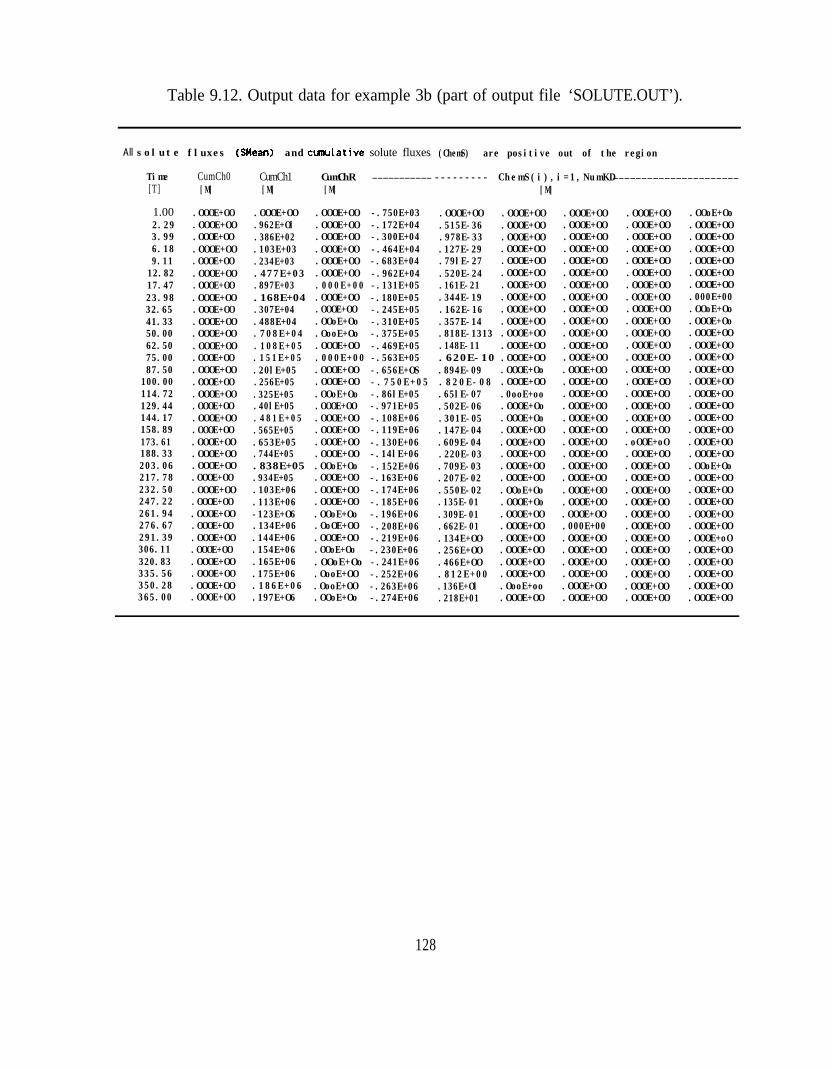
Table 9.12. Output data for example 3b (part of output file ‘SOLUTE.OUT’).

All solute fluxes Wean) and cunulative solute fluxes

Time[T]

1.002.293.996.189.1112.8217.4723.9832.6541.3350.0062.5075.0087.50100.00114.72129.44144.17158.89173.61188.33203.06

CumCh0 CumCh1 CumChR ___________[M] [M] [M]

.OOOE+OO .OOOE+OO .OOOE+OO -.750E+03

.OOOE+OO .962E+Ol .OOOE+OO -.172E+04

.OOOE+OO .386E+02 .OOOE+OO -.300E+04

.OOOE+OO .103E+03 .OOOE+OO -.464E+04

.OOOE+OO .234E+03 .OOOE+OO -.683E+04

.OOOE+OO .477E+03 .OOOE+OO -.962E+04

.OOOE+OO .897E+03 .000E+00 -.131E+05

.OOOE+OO .168E+04 .OOOE+OO -.180E+05

.OOOE+OO .307E+04 .OOOE+OO -.245E+05

.OOOE+OO .488E+04 .OOoE+Oo -.310E+05

.OOOE+OO .708E+04 .OooE+Oo -.375E+05

.OOOE+OO .108E+05 .OOOE+OO -.469E+05

.OOOE+OO .151E+05 .000E+00 -.563E+05

.OOOE+OO .20lE+05 .OOOE+OO -.656E+OS

.OOOE+OO .256E+05 .OOOE+OO -.750E+05

.OOOE+OO .325E+05 .OOoE+Oo -.86lE+05

.OOOE+OO .40lE+05 .OOOE+OO -.971E+05

.OOOE+OO .481E+05 .OOOE+OO -.108E+06

.OOOE+OO .565E+05 .OOOE+OO -.119E+06

.OOOE+OO .653E+05 .OOOE+OO -.130E+06

.OOOE+OO .744E+05 .OOOE+OO -.14lE+06

.OOOE+OO .838E+05 .OOoE+Oo -.152E+06

.OOOE+OO .934E+05 .OOOE+OO -.163E+06

.OOOE+OO .103E+06 .OOOE+OO -.174E+06

.OOOE+OO .113E+06 .OOOE+OO -.185E+06

.OOOE+OO -123E+O6 .OOoE+Oo -.196E+06

.OOOE+OO .134E+06 .OoOE+OO -.208E+06

.OOOE+OO .144E+06 .OOOE+OO -.219E+06

.OOOE+OO .154E+06 .OOoE+Oo -.230E+06

.OOOE+OO .165E+06 .OOoE+Oo -.241E+06

.OOOE+OO .175E+06 .OooE+OO -.252E+06

.OOOE+OO .186E+06 .OooE+OO -.263E+06

.OOOE+OO .197E+O6 .OOoE+Oo -.274E+06

217.78232.50247.22261.94276.67291.39306.11320.83335.56350.28365.00

(ChemS) are positive out of the region

--------- ChemS(i),i=1,NumKD______________________[M]

.OOOE+OO .OOOE+OO .OOOE+OO .OOOE+OO .OOoE+Oo

.515E-36 .OOOE+OO .OOOE+OO .OOOE+OO .OOOE+OO

.978E-33 .OOOE+OO .OOOE+OO .OOOE+OO .OOOE+OO

.127E-29 .OOOE+OO .OOOE+OO .OOOE+OO .OOOE+OO

.79lE-27 .OOOE+OO .OOOE+OO .OOOE+OO .OOOE+OO

.520E-24 .OOOE+OO .OOOE+OO .OOOE+OO .OOOE+OO

.161E-21 .OOOE+OO .OOOE+OO .OOOE+OO .OOOE+OO

.344E-19 .OOOE+OO .OOOE+OO .OOOE+OO .000E+00

.162E-16 .OOOE+OO .OOOE+OO .OOOE+OO .OOoE+Oo

.357E-14 .OOOE+OO .OOOE+OO .OOOE+OO .OOOE+Oo

.818E-1313 .OOOE+OO .OOOE+OO .OOOE+OO .OOOE+OO

.148E-11

.620E-10.OOOE+OO .OOOE+OO .OOOE+OO .OOOE+OO.OOOE+OO .OOOE+OO .OOOE+OO .OOOE+OO

.894E-09 .OOOE+Oo .OOOE+OO .OOOE+OO .OOOE+OO

.820E-08 .OOOE+OO .OOOE+OO .OOOE+OO .OOOE+OO

.65lE-07 .0ooE+oo .OOOE+OO .OOOE+OO .OOOE+OO

.502E-06 .OOOE+Oo .OOOE+OO .OOOE+OO .OOOE+OO

.301E-05 .OOOE+Oo .OOOE+OO .OOOE+OO .OOOE+OO

.147E-04 .OOOE+OO .OOOE+OO .OOOE+OO .OOOE+OO

.609E-04 .OOOE+OO .OOOE+OO .oOOE+oO .OOOE+OO

.220E-03 .OOOE+OO .OOOE+OO .OOOE+OO .OOOE+OO

.709E-03 .OOOE+OO .OOOE+OO .OOOE+OO .OOoE+Oo

.207E-02 .OOOE+OO .OOOE+OO .OOOE+OO .OOOE+OO

.550E-02 .OOoE+Oo .OOOE+OO .OOOE+OO .OOOE+OO

.135E-01 .OOOE+Oo .OOOE+OO .OOOE+OO .OOOE+OO

.309E-01 .OOOE+OO .OOOE+OO .OOOE+OO .OOOE+OO

.662E-01 .OOOE+OO .000E+00 .OOOE+OO .OOOE+OO

.134E+OO .OOOE+OO .OOOE+OO .OOOE+OO .OOOE+oO

.256E+OO .OOOE+OO .OOOE+OO .OOOE+OO .OOOE+OO

.466E+OO .OOOE+OO .OOOE+OO .OOOE+OO .OOOE+OO

.812E+00 .OOOE+OO .OOOE+OO .OOOE+OO .OOOE+OO

.136E+Ol .OooE+oo .OOOE+OO .OOOE+OO .OOOE+OO

.218E+01 .OOOE+OO .OOOE+OO .OOOE+OO .OOOE+OO

128

Table 9.13. Output data for example 3b (output file ‘BALANCE.OUT’).

Example 3b - Comparison with the 3-D analytical solution

Program SUMS_3DDate: 1. 3. Time: 16:10:17Time independent boundary conditionsUnits: L = m , T = days , M q -

Time [T]

. 0000Volume [L3]Water IL31Inflow [L3/T]hMean [L]ConcVol [M]cMean [M/L3]

50.0000Volume CL31Water [L3]Inflow [L3/T]hMean [ L ]ConcVol [M]cMean [M/L3]CncBalT [ M ] -CncBalR [%]

Total Sub-region nunber . . .

1.288E+07 .288E+07.864E+06 .864E+06.OOOE+OO .OOOE+OO.OOOE+OO .0.OOOE+OO .O00E+O0.OOOE+OO .OOOE+OO

I.288E+07 .288E+07.864E+06 .864E+06.0OOE+OO .OOOE+OO.OOOE+OO .O.295E+05 .295E+05.114E-01 .114E-01'.900E+03

2.018

100.0000 IVolume [L3] .288E+07 .288E+07ConcVol [M] .474E+05 .474E+05cMean [M/L3] .l83E-01 .l83E-01CncBalT [M] - .202E+04CncBalR [%] 2.009

365.0000 IVolume [L3] .288E+07 .288E+07ConcVol [M] .731E+05 .731E+05cMean [M/L3] .282E-01 .282E-01CncBalT [M] -.393E+04CncBalR [%] .835

129

TABLE 9.14. Output data for example 3b (part of output file ‘CONC.OUT’).

Time l ** 365.0000 l **

n x(n) y(n)

1 .o .o11 67.0 .O21 45.0 10.031 .o 20.041 67.0 20.051 45.0 30.061 .o 40.071 67.0 40.081 45.0 45.091 .o 49.0101 67.0 49.0111 45.0 51.0121 .o 55.0131 67.0 55.0141 45.0 60.0151 .O 67.0161 67.0 67.0171 45.0 75.0181 .O 85.0191 67.0 85.0201 45.0 100.0211 .o 120.0221 67.0 120.0226 .O .O236 67.0 .O246 45.0 10.0256 .o 20.0266 67.0 20.0276 45.0 30.0286 .o 40.0296 67.0 40.0306 45.0 45.0316 .o 49.0326 67.0 49.0336 45.0 51.0346 .o 55.0356 67.0 55.0366 45.0 60.0376 .O 67.0386 67.0 67.0396 45.0 75.0406 .O 85.0416 67.0 85.0426 45.0 100.0436 .o 120.0446 67.0 120.0

z(n) Conc(n)Conc(n+l) . .

.O .97OE+OO .971E+OO .97OE+OO .971E+OO .969E+OO .965E+OO .88OE+OO .128E+OO -.453E-02 -125E-03

.O -.169E-03 .268E-O4 .235E-04 -.275E-O6 .273E-05 .97lE+OO .970E+OO .97lE+OO .97OE+OO .971E+OO

.O .974E+OO .843E+OO .899E-01 .589E-O2 .106E-02 -.593E-04 -.309E-04 -.528E-05 -.754E-05 .109E-05

.O .97OE+OO .971E+OO .97OE+OO .97lE+OO .969E+OO .965E+OO .88OE+OO .128E+OO -.454E-02 -.125E-O3

.O -.183E-03 .284E-04 .290E-O4 -.67lE-O6 .939E-O6 .97lE+OO .97OE+OO .971E+OO .97OE+OO .97lE+OO

.O .975E+OO .843E+OO .901E-01 .589E-O2 .1l4E-02 -.675E-O4 -.582E-04 -.358E-05 -.519E-05 .970E-06

.O .969E+OO .97lE+OO .969E+OO .97lE+OO .968E+OO .966E+OO .878E+OO .127E+OO -.539E-02 -.905E-04

.O -.474E-04 ,192E-04 .207E-O4 ~564E-06 .500E-O6 .965E+OO .974E+OO .965E+OO .975E+OO .966E+OO

.O .983E+OO .843E+OO .994E-01 .480E-02 .108E-O3 -.292E-04 -.251E-04 -.57lE-06 -.236E-05 .353E-06

.O .88OE+OO .843E+OO .88OE+OO .843E+OO .878E+OO .843E+OO .786E+OO .105E+OO -.529E-02 -.167E-03

.O .106E-O3 .243E-O5 .150E-O5 -.829E-O7 .876E-06 .128E+OO .899E-01 .128E+OO .901E-01 .127E+OO

.O .994E-01 .105E+OO .286E-01 .2.50E-03 -.693E-O3 .620E-05 .696E-05 .382E-06 .149E-06 .142E-06

.O -.453E-O2 .589E-O2 -.454E-O2 .589E-02 -.539E-02 .480E-O2 -.529E-02 .250E-03 -.393E-03 -.442E-04

.O .306E-05 .138E-O5 .122E-O5 -.378E-07 -.llOE-O6 -.125E-03 .106E-02 -.125E-03 .114E-02 -.905E-04

.O .108E-O3 -.167E-03 -.693E-03 -.442E-O4 .173E-O4 .139E-05 .153E-O5 -.189E-06 -.270E-06 .156E-07

.O -.169E-03 -.593E-O4 -.183E-03 -.675E-O4 -.474E-O4 -.292E-04 .106E-03 .620E-05 .306E-05 .139E-05

.O .155E-O5 -.489E-06 -.733E-O6 .660E-O7 .209E-06 .268E-O4 -.309E-04 .284E-04 -.582E-O4 .192E-04

.O -.251E-04 243E-05 .696E-05 .138E-05 .153E-05 -.489E-06 -.108E-O5 .151E-O6 .207E-06 -.478E-07

.O .235E-04 -.528E-O5 .29OE-O4 -.358E-O5 .207E-04 -.571E-O6 .150E-O5 .382E-O6 .122E-05 -.189E-06

.O -.733E-06 .l5lE-06 337E-06 -.338E-07 -.171E-06 -.275E-06 -.754E-05 -.67lE-06 -.519E-05 -.564E-06

.O -.236E-O5 -.829E-O7 .149E-O6 -.378E-07 -.270E-06 .66OE-O7 .207E-06 -.338E-07 -.457E-07 .158E-07

.O .273E-05 .109E-05 .939E-06 .97OE-O6 .5OOE-O6 .353E-06 .876E-06 .142E-06 -.llOE-06 .156E-O7

.O .209E-O6 -.478E-O7 -.17lE-O6 .158E-O7 .117E-O6-5.0 .842E+OO .838E+OO .842E+OO .836E+OO .84lE+OO .849E+OO .602E+OO .279E+OO .437E-01 -.475E-03-5.0 -.298E-03 -.52lE-O3 .257E-04 .328E-O5 .382E-O5 .838E+OO .842E+OO .838E+OO .842E+OO .838E+OO-5.0 .797E+OO .559E+OO .238E+OO -.113E-O1 .352E-03 .138E-02 .146E-04 .96OE-O4 -.lllE-04 -.183E-04-5.0 .842E+OO .838E+OO .842E+OO .837E+OO .841E+OO .85OE+OO .602E+OO .279E+OO .437E-01 -.49lE-03-5.0 -.307E-03 ~557E-03 .304E-04 .107E-O4 .169E-05 .836E+OO .842E+OO .837E+OO .842E+OO .837E+OO-5.0 .797E+OO .559E+OO 238E+OO -.lllE-Ol .412E-03 .157E-02 -.527E-05 .626E-04 -.807E-05 -.166E-04-5.0 .84lE+OO .838E+OO .841E+OO .837E+OO .841E+OO .848E+OO .599E+OO .276E+OO .40lE-01 -.163E-02-5.0 ~155E-03 -.383E-O3 225E-04 .838E-05 .500E-06 .849E+OO .797E+OO .850E+OO .797E+OO .848E+OO-5.0 .777E+OO .57OE+OO 243E+OO .2llE-O2 .153E-03 .686E-03 -.492E-04 .280E-04 -.195E-05 -.530E-05-5.0 .602E+OO .559E+OO .602E+OO .559E+OO .599E+OO .57OE+OO .423E+OO .186E+OO .182E-01 -.187E-02-5.0 .780E-04 -.477E-O4 .523E-05 -.164E-05 -.365E-Q6 .279E+OO .238E+OO .279E+OO .238E+OO .276E+OO-5.0 .243E+OO .186E+OO .967E-01 .656E-O2 -.45lE-03 .572E-06 -.186E-04 -.292E-06 -.516E-06 -.254E-06-5.0 .437E-01 -.113E-O1 .4378-01 -.lllE-Ol ,401E-Ol .2llE-02 .182E-01 .656E-02 .16lE-02 -.15lE-03-5.0 -.188E-04 ~166E-04 .144E-O5 .690E-O6 -.116E-06 -.475E-03 .352E-O3 -.49lE-03 .412E-03 -.163E-02-5.0 .153E-O3 ~187E-02 -.451E-O3 -.15lE-03 -.331E-O4 -.168E-04 .173E-05 .412E-O5 -.309E-06 -.262E-06-5.0 -.298E-O3 .138E-O2 -.307E-O3 .157E-O2 -.155E-03 .686E-03 .780E-04 .572E-06 -.188E-04 ~168E-o04-5.0 .397E-05 .933E-05 -.971E-O6 -.123E-O5 .289E-O6 -.52lE-03 .146E-O4 -.557E-03 -.527E-05 -.383E-O3-5.0 -.492E-04 -.477E-O4 -.186E-04 -.166E-O4 .173E-05 .933E-05 -.141E-05 -.289E-O5 .310E-O6 .851E-06-5.0 .257E-04 .960E-O4 .304E-04 .626E-O4 .225E-04 .280E-04 .523E-05 -.292E-06 .144E-05 .412E-05-5.0 -.971E-06 -.289E-O5 .473E-06 .61lE-06 -.266E-06 .328E-05 -.lllE-04 .107E-04 -.807E-05 .838E-05-5.0 -.195E-05 -.164E-05 -.516E-06 .690E-06 -.309E-06 -.123E-05 .310E-06 .6llE-06 -.828E-07 -.271E-06-5.0 .382E-05 -.183E-O4 .169E-05 -.166E-04 .500E-06 -.530E-05 -.365E-06 -.254E-06 -.116E-06 -.262E-06-5.0 .289E-06 .851E-O6 -.266E-06 -.271E-06 .205E-06

451 .o .O -10.0 .724E+OO .727E+OO .724E+OO .726E+OO .733E+OO .69OE+OO .47OE+OO .29OE+OO .453E-01 .487E-02461 67.0 .O -10.0 .185E-02 -.380E-03 -.117E-03 .5lOE-05 -.234E-04 .727E+OO .725E+OO .727E+OO .723E+OO .723E+OO

130

Table 9.15. Output data for example 4 (output file ‘CUM_Q.OUT’).

Example 4 - Contaminant Transport from a Waste Disposal Site in a Pumped Aquifer

Program SUMS-30Date: 6. 3. Time: 15:50:52Time independent boundary conditionsUnits: L = cm , T = day , M = -All cumulative fluxes (CumQ) are positive out of the region

Time[T]

CumQAP[L3]

.2500 .OOOE+OO1.5000 .OOOE+OO5.0000 .OO0E+0O10.0000 .O0OE+OO20.0000 .OOOE+OO30.0000 .OOOE+OO50.0000 .OOOE+OO

100.0000 .OOOE+OO200.0000 .OOOE+OO

CumQRP[L3]

.OOOE+OO

.OOOE+OO

.OOOE+OO

.0OOE+OO .OOOE+0O.OOOE+OO.OOOE+OO.OOOE+OO.OOOE+0O

CumQA[L3]

.OOOE+OO

.OOOE+OO

.OOOE+OO

.OOOE+OO

.OOOE+OO

.OOOE+O0

.OOOE+OO

.OOOE+OO

.OOOE+OO

CumQR[L3]

.OOOE+0O

.OOOE+OO

.OOOE+OO

.OO0E+OO

.OOOE+OO

.OOOE+OO

.OOOE+OO

.OOOE+OO

.OOOE+OO

CumQ3 CumQ1[L3] [L3]

.OOOE+OO -.671E+02

.OOOE+OO -.730E+03

.0OOE+OO -.129E+O4

.OOOE+OO -.135E+04

.O0OE+OO -.166E+04

.OOOE+OO -.198E+04

.OOOE+OO -.240E+04

.OOOE+OO -.322E+04

.OOOE+OO -.475E+04

CumQS[L3]

.297E+02

.123E+03

.257E+O3

.372E+03

.532E+03

.680E+03

.984E+03

.175E+04

.330E+04

CumQ5[L3]

.OOOE+OO

.OOOE+OO

.OOOE+OO

.OO0E+OO

.OOOE+OO

.OOOE+OO

.O0OE+OO

.OOOE+OO

.OOOE+OO

CumQ6[L3]

.OOOE+OO

.OOOE+OO

.OOOE+OO

.OOOE+OO

.OOOE+OO

.OOOE+OO

.OOOE+OO

.OOOE+OO

.OOOE+OO

131

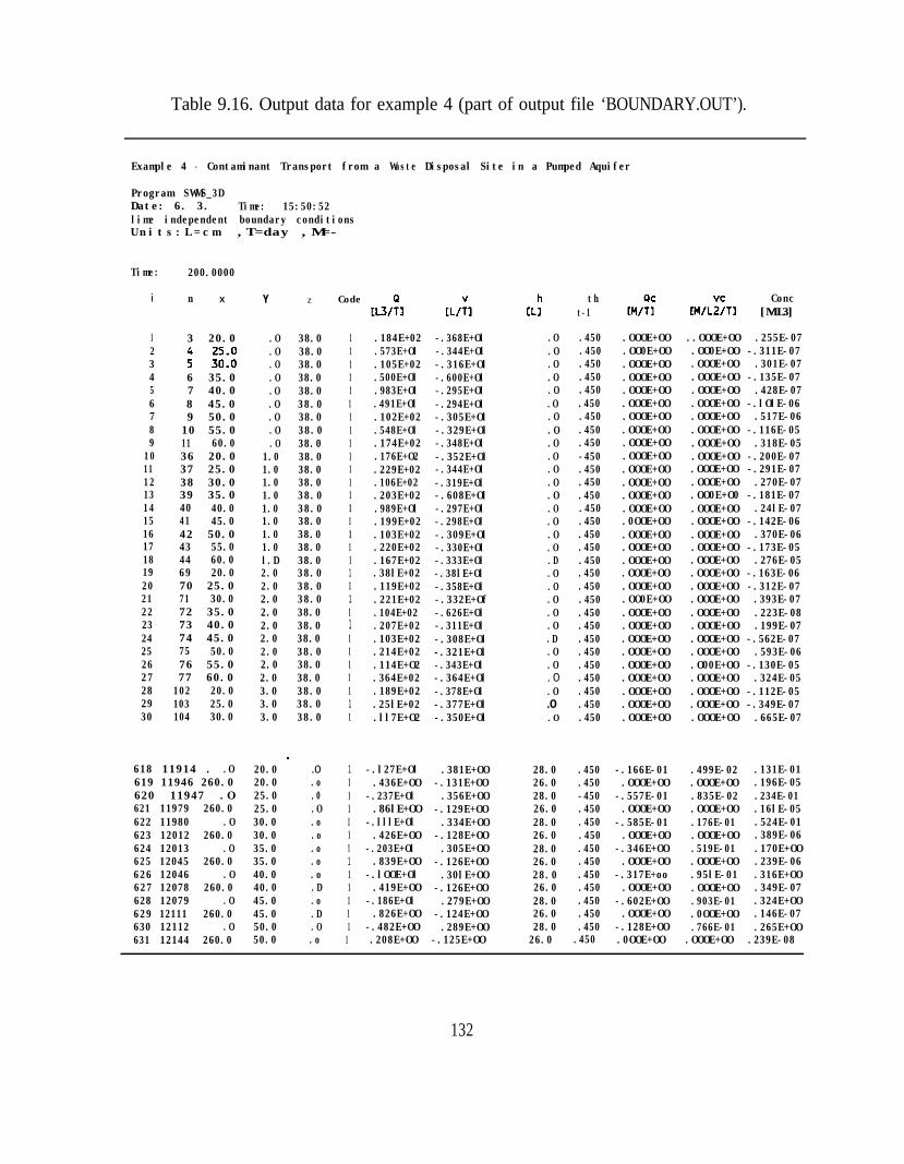
Table 9.16. Output data for example 4 (part of output file ‘BOUNDARY.OUT’).

Example 4 - Contaminant Transport from a Waste Disposal Site in a Pumped Aquifer

Program SWMS_3DDate: 6. 3. Time: 15:50:52lime independent boundary conditionsU n i t s : L = c m ,T=day ,M=-

Time:

i

123456789

101112131415161718192021222324252627282930

200.0000

n X

3 20.0

: z::6 35.07 40.08 45.09 50.010 55.011 60.036 20.037 25.038 30.039 35.040 40.041 45.042 50.043 55.044 60.069 20.070 25.071 30.072 35.073 40.074 45.075 50.076 55.077 60.0102 20.0103 25.0104 30.0

Code

1 .184E+02 -.368E+Ol1 .573E+Ol -.344E+Ol1 .105E+02 -.316E+Ol1 .500E+Ol -.600E+Ol1 .983E+Ol -.295E+Ol1 .491E+Ol -.294E+Ol1 .102E+02 -.305E+Ol1 .548E+Ol -.329E+Ol1 .174E+02 -.348E+Ol

IL:

.O

.O

.O

.O

.O

.O

.O

.O

.O

.O

.O

.O

.O

.O

.O

.O

.O

.D

.O

.O

.O

.O

.O

.D

.O

tht-1 WL~STI

Conc[M/L3]

.450 .OOOE+OO ..OOOE+OO .255E-07

.450 .OO0E+OO .OO0E+OO -.311E-07

.450 .OOOE+OO .OOOE+OO .301E-07

.450 .OOOE+OO .OOOE+OO -.135E-07

.450 .OOOE+OO .OOOE+OO .428E-07

Y z

.O 38.0

.O 38.0

.O 38.0

.O 38.0

.O 38.0

.O 38.0

.O 38.0

.O 38.0

.O 38.01.0 38.01.0 38.01.0 38.01.0 38.01.0 38.01.0 38.01.0 38.01.0 38.0l.D 38.02.0 38.02.0 38.02.0 38.02.0 38.02.0 38.02.0 38.02.0 38.02.0 38.02.0 38.03.0 38.03.0 38.03.0 38.0

-20.0 .o20.0 .o25.0 .025.0 .O30.0 .o30.0 .o35.0 .o35.0 .o40.0 .o40.0 .D45.0 .o45.0 .D50.0 .O50.0 .o

.450 .OOOE+OO .OOOE+OO -.lOlE-06

.450 .OOOE+OO .OOOE+OO .517E-06

.450

.450.OOOE+OO.OOOE+OO.OOOE+OO.OOOE+OO.OOOE+OO.OOOE+OO.OOOE+OO.0OOE+OO

.OOOE+OO -.116E-05

.OOOE+OO .318E-05

.OOOE+OO -.200E-07

.OOOE+OO -.291E-07

.OOOE+OO .270E-07

1 .176E+O2 -.352E+Ol1 .229E+02 -.344E+Ol

-450.450

1 .106E+021 .203E+021 .989E+Ol1 .199E+02

-.319E+Ol-.608E+Ol-.297E+Ol-.298E+Ol-.309E+Ol-.330E+Ol-.333E+Ol-.38lE+Ol-.358E+Ol-.332E+Of-.626E+Ol-.311E+Ol-.308E+Ol-.321E+Ol-.343E+Ol-.364E+Ol-.378E+Ol-.377E+Ol-.350E+Ol

.450

.450

.450.OO0E+O0 -.181E-07.OOOE+OO .24lE-07.OOOE+OO -.142E-06.450

1 .103E+021 .220E+02

.450 .OOOE+OO .OOOE+OO .370E-06

.450 .OOOE+OO .OOOE+OO -.173E-051 .167E+02 .450

.450

.450

.450

.OOOE+OO .OOOE+OO .276E-05

.OOOE+OO .OOOE+OO -.163E-06

.OOOE+OO .OOOE+OO -.312E-07

.OO0E+OO .OOOE+OO .393E-07

.OOOE+OO .OOOE+OO .223E-08

.OOOE+OO .OOOE+OO .199E-07

.OOOE+OO .OOOE+OO -.562E-07

.OOOE+OO .OOOE+OO .593E-06

.OOOE+OO .O00E+OO -.130E-05

.OOOE+OO .OOOE+OO .324E-05

.OOOE+OO .OOOE+OO -.112E-05

.OOOE+OO .OOOE+OO -.349E-07

.OOOE+OO .OOOE+OO .665E-07

1 .38lE+021 .119E+021 .221E+021 .104E+021 .207E+02

.450

.4501 .103E+021 .214E+021 .114E+O21 .364E+021 .189E+02

.450

.450

.450

.450

.450

.O

. O

.O.O.O

1 .25lE+021 .ll7E+O2

.450

.450

618 11914 . .O619 11946 260.0620 11947 .O

1 -.l27E+Ol1 .436E+OO1 -.237E+Ol1 .86lE+OO1 -.lllE+Ol

.381E+OO-.131E+OO.356E+OO

-.129E+OO.334E+OO

-.128E+OO.305E+OO

-.126E+OO.30lE+OO

-.126E+OO.279E+OO

-.124E+OO.289E+OO

-.125E+OO

28.026.028.026.028.026.028.026.028.026.028.026.028.026.0

.450

.450-450.450.450.450.450.450

-.166E-01 .499E-02 .131E-01.OOOE+OO .OOOE+OO .196E-05

-.557E-01 .835E-02 .234E-01.OOOE+OO .OOOE+OO .16lE-05

-.585E-01 .176E-01 .524E-01.OOOE+OO .OOOE+OO .389E-06

-.346E+OO .519E-01 .170E+OO.OOOE+OO .OOOE+OO .239E-06

-.317E+oo .95lE-01 .316E+OO.OOOE+OO .OOOE+OO .349E-07

-.602E+OO .903E-01 .324E+OO.OOOE+OO .0OOE+OO .146E-07

-.128E+OO .766E-01 .265E+OO.0OOE+OO .OOOE+OO .239E-08

621 11979 260.0622 11980 .O623 12012 260.0624 12013 .O625 12045 260.0626 12046 .O627 12078 260.0628 12079 .O629 12111 260.0630 12112 .O631 12144 260.0

1 .426E+OO1 -.203E+Ol1 .839E+OO1 -.lOOE+Ol1 .419E+OO1 -.186E+Ol1 .826E+OO1 -.482E+OO1 .208E+OO

.450

.450

.450

.450

.450.450

132

10. PROGRAM ORGANIZATION AND LISTING

10.1. Description of Program Units

The program consists of a main program and 61 subprograms. The subprograms are

organized by means of 8 source files which are stored and compiled separately and then linked

together with the main program to form an executable program. Below are a list and brief

descriptions of the source files and the associated subprograms.

SWMS_3D.FOR

INPUT3 .FOR

WATFLOW3.FOR

TIME3 .FOR

MATERIA3 .FOR

SINK3.FOR

OUTPUT3.FOR

SOLUTE3.FOR

ORTHOFEM.FOR

(Main program unit)

BasInf, MatIn, GenMat, TmIn, SeepIn, NodInf, EIemIn, GeomIn, AtmIn,SinkIn, ChemIn, DrainIn, Elem

WatFIow, Reset, Dirich, Solve, Shift, SetMat, Veloc

TmCont, SetAtm, Fgh

FK, FC, FQ, FH

SetSnk, FAlfa

TLInf, ALInf, hOut, thOut, QOut, FIxOut, SubReg, BouOut, cOut,SolInf, ObsNod

Solute, cBound, ChInit, Disper, SolveT, WeFact, PeCour

IADMake, Insert, Find, ILU, DU, ORTHOMIN, LUSolv, MatM2, SDot,SDotK, SNRM, SAXPYK, SCopy, SCopyK

Main program unit SWMS_3D. FOR

This is the main program unit of SWMS_3D. This unit controls execution of the program

and determines which optional subroutines are necessary for a particular application.

133

Source file INPUT3. FOR

Subroutines included in this source file are designed to read data from different input

blocks. The following table summarizes from which input file and input block (described in

Section 8) a particular subroutine reads.

Table 10.1. Input subroutines/files.

Subroutine Input Block Input File

BasInfMatInTmInSinkInSeepInDrainInChemIn

NodInfElemInGeomIn

AtmIn

A.B.C.D.E.F.G.

H.I.J.

K.

Basic InformationMaterial InformationTime InformationSink InformationSeepage InformationDrain InformationSolute Transport Information

Nodal InformationElement InformationBoundary Geometry Information

Atmospheric Information

SELECTOR.IN

GRID.IN

ATMOSPH.IN

Subroutine GenMat generates for each soil type in the flow domain a table of water contents,hydraulic conductivities, and specific water capacities from the set of hydraulic parameters.

Subroutine Elem subdivides the input hexahedral and triangular prismatic elements intotetrahedrals which are subsequently treated as subelements.

Source file WATFLOW3. FOR

Subroutine WatFlow is the main subroutine for simulating water flow; this subroutine controlsthe entire iterative procedure of solving the Richards equation.

Subroutine Reset constructs the global matrix equation for water flow, including the right-handside vector.

134

Subroutine Dirich modifies the global matrix equation by incorporating prescribed pressure headnodes.

Subroutine Solve solves the banded symmetric matrix equation for water flow by Gaussianelimination.

Subroutine Shift changes atmospheric or seepage face boundary conditions from Dirichlet typeto Neumann type conditions, or vice versa, as needed. Also updates boundary conditions for thevariable boundary fluxes (free and deep drainage).

Subroutine SetMat determines the nodal values of the hydraulic properties K(h), C(h) and 6(h)by interpolation between intermediate values in the hydraulic property tables.

Subroutine Veloc calculates nodal water fluxes.

Source file TIME3. FOR

Subroutine TmCont adjusts the current value of the time increment At.

Subroutine SetAtm updates time-dependent boundary conditions.

Function Fqh describes the groundwater level - discharge relationship, q(h), defined by equation(6.1). This function is called only from subroutine SetAtm.

Source file MA TERIA3. FOR

This file includes the functions FK, FC, FQ and FH which define the unsaturated

hydraulic properties K(h), C(h), 19(h), and h(8), for each soil material.

Source file SINK3. FOR

This file includes subroutine SetSnk and function FAlfa. These subroutines calculate the

135

actual root water extraction rate as a function of water stress in the soil root zone.

Source file OUTP UT3. FOR

The subroutines included in this file are designed to print data to different output files.

Table 10.2 summarizes which output files are generated by a particular subroutine.

Table 10.2. Output subroutines/files.

Subroutine Output File

TLInf

SolInf

hOut

thout

cOut

QOut

FlxOut

BouOut

SubReg

ALInf

ObsNod

H_MEAN.OUTV_MEAN.OUTCUM_Q.OUTRUN_INF.OUT

SOLUTE.OUT

H.OUT

TH.OUT

CONC.OUT

Q.OUT

VX.OUTVY.OUTVZ.OUT

BOUNDARY.OUT

BALANCE.OUT

A_LEVEL.OUT

OBSNOD.OUT

Source file SOL UTE3. FOR

Subroutine Solute is the main subroutine for simulating solute transport; it constructs the globalmatrix equation for transport, including the right-hand side vector.

Subroutine c-Bound determines the values of the solute transport boundary codes, cKod(n), and

136

incorporates prescribed boundary conditions in the global matrix equation for solute transport.

Subroutine ChInit initializes selected transport parameters at the beginning of the simulation.

Subroutine Disper calculates nodal values of the dispersion coefficients.

Subroutine SolveT solves theGaussian elimination.

final asymmetric banded matrix equation for solute transport using

Subroutine WeFact computes the optimum

Subroutine PeCour computes the maximumpermissible time step.

Source file ORTHOFEM. FOR

weighing factors for all sides of all elements.

local Peclet and Courant numbers and the maximum

The subroutines included in this file solve large sparse systems of linear algebraic

equations using the preconditioned conjugate gradient method for symmetric matrices, and the

ORTHOMTN method for asymmetric matrices. The subroutines were adopted from Mendoza et

al. [ 1991] (see Mendoza et al. [ 1991] for a detailed description of both methods).

Subroutine IADMake generates the adjacency matrix which determines nodal connections fromthe finite element incidence matrix.

Subroutine Insert adds node j to the adjacency list for node i.

Subroutine Find retrieves from the adjacency matrix the appropriate position of two global pointsin the coefficient matrix.

Subroutine ILU performs incomplete lower-upper decomposition of matrix [A].

Function DU searches the ith row of the upper diagonal matrix for an adjacency of node j.

Subroutine ORTHOMIN governs the ORTHOMIN (conjugate gradient) acceleration.

Subroutine LUSolv performs lower diagonal matrix inversion by forward substitution, and upperdiagonal matrix inversion by backward substitution.

137

Subroutine MatM2 multiplies a matrix by a vector.

Function SDot calculates the dot product of two vectors.

Function SDotK calculates the dot product of a column in matrix by a vector.

Function SNRM computes the maximum norm of a vector.

Subroutine SAXPYK multiplies a column in a matrix by a scalar, and adds the resulting valueto another vector.

Subroutine SCopy copies a vector into another vector.

Subroutine SCopyK copies a column in a matrix into a vector.

Source file GENER3. FOR

In addition to the main code SWMS_3D, we also provide a simple mesh generator,

GENER3, which may be used to generate the input file GRID.IN for simple hexahedral flow

regions. Generator assumes that the local anisotropy is the same throughout the flow region and

that the initial pressure head and concentration, as well as the scaling factors, root distribution,

material numbers, recharge/discharge and boundary codes are all the same within a particular

horizontal layer. If this is not the case, then the user must modify the resulting output file

GRID.IN manually or with available word- or data-processing software. The source code is

stored in the source file GENER3.FOR. The GENER3 code reads input file GENER3.IN, which

must be included, as well as other input files for SWMS_3D, in subdirectory SWMS_3D.lN.

138

10.2. List of Significant SWMS_3D Program Variables.

Variables which appear in subroutines of the ORTHOFEM package are not given in

following tables. Consult the user’s guide of ORTHOFEM [Mendoza et al., 1991] for their

definition.

Table 10.3. List of significant integer variables.

ALevel

cKod

IJ

ItCum

Iter

MaxAl

MaxIt

MBand

MBandD

MPL

NDr

NDrD

NLay

NLevel

NMat

NMatD

NObs

NObsD

NPar

NSeep

Time level at which a time-dependent boundary condition is specified.

Code which specifies the type of boundary condition used for solute transport.

Maximum number of nodes on any transverse line (Table 8.8).

Cumulative number of iterations (Table 9.4).

Number of iterations (Table 9.4).

Number of atmospheric data records (Table 8.11).

Maximum number of iterations allowed during any time step for the solution of water flowequation (Table 8.1).

Bandwidth (or half-bandwidth) of the symmetric (or asymmetric) matrix A when Gaussianelimination is used. Maximum number of nodes adjacent to another node when iterative solversare used.

Maximum permitted bandwidth of matrix A when Gaussian elimination is used. Maximumpermitted number of nodes adjacent to another node when iterative solvers are used (Table 6.7).

Number of specified print-times at which detailed information about the pressure head, the watercontent, flux, concentration, and the soil water and solute balances is printed (Table 8.3).

Number of drains.

Maximum permitted number of drains.

Number of subregions for which separate water balances are being computed (Table 8.2).

Number of time levels at which matrix A and vector B are assembled for solute transport.

Number of soil materials (Table 8.2).

Maximum permitted number of soil materials (Table 6.7).

Number of observation nodes for which values of the pressure head, water content, andconcentration are printed at each time level.

Maximum number of observation nodes for which values of pressure head, water content, andconcentration are printed at each time level.

Number of unsaturated soil hydraulic parameters specified for each material (Table 8.2).

Number of seepage faces expected to develop (Table 8.5).

139

Table 10.3. (continued)

NSeepD

NTab

NTabD

NumBP

NumBPD

NumEl

NumElD

NumKD

NumNP

NumNPD

NumSEl

NumSPD

NUS

PLevel

TLevel

Maximum permitted number of seepage faces (Table 6.7).

Number of entries in the internally generated tables of the hydraulic properties (see Section 4.3.11).

Maximum permitted number of entries in the internally generated tables of the hydraulic properties(Table 6.7).

Number of boundary nodes for which Kode(N) f 0 (Table 8.8).

Maximum permitted number of boundary nodes for which Kode(n) f 0 (Table 6.7).

Number of elements (tetrahedrals, hexahedrals, and/or triangular prisms) (Table 8.8).

Maximum permitted number of elements in finite element mesh (Table 6.7).

Maximum permitted number of available code number values (Table 6.7).

Number of nodal points (Table 8.8).

Maximum permitted number of nodes in finite element mesh (Table 6.7).

Number of subelements (tetrahedrals).

Maximum number of nodes along a seepage face (Table 6.7).

Number of comer nodes of a particular element.

Print time-level (current print-time number).

Time-level (current time-step number) (Table 9.4).

140

Table 10.4. List of significant real variables.

AlfAlfa

Aqh

Bqh

cBalR

cBalT

cBnd

cCumA

cCumT

cE

Change

cht

cNewE

ConA 1

conA2

ConA3

con Vol

Cos11

cos22

cos33

cos12

Cosl3

cos23

Courant

1-Epsi, where Epsi is a temporal weighing coefficient [-].

Parameter in the soil water retention function &‘I (see Section 2.3).

Parameter A, in equation (6.1) [LT’] (Table 8.11).

Parameter B, in equation (6.1) [L’] (Table 8.11).

Relative error in the solute mass balance of the entire flow domain [%] (see equation (5.31))(CncBalR in Table 9.6).

Absolute error in the solute mass balance of the entire flow domain [M] (see equation (5.30))(CncBalT in Table 9.6).

Value of the boundary condition for solute transport [ML^-3].

Sum of the absolute values of all cumulative solute fluxes across the flow boundaries, includingthose resulting from sources and sinks in the flow domain [M] (see equation (5.3 1)).

Sum of all cumulative solute fluxes across the boundaries, including those resulting from sourcesand sinks in the flow domain [M] (see right hand side of equation (5.30)).

Average concentration of an element [ML^-3].

Inflow/Outflow to/from the flow domain [L’T’] (InFlow in Table 9.6).

Time-dependent concentration for the first-type boundary condition assigned to nodes for whichKode(n)=+3 [ML”] (Table 8.11).

Amount of solute in a particular element at the new time-level [M].

First principal component, K,*, of the dimensionless anisotropy tensor KA [-] assigned to eachelement (Table 8.9).

Second principal component, K,A of KA [-] (Table 8.9).

Third principal component, K,A of K” [-] (Table 8.9).

Amount of solute in the entire flow domain [M] (ConVol in Table 9.6).

Cosine of an angle between the principal direction of K,” and the x-axis of the global coordinatesystem assigned to each element (Table 8.9).

Cosine of an angle between the principal direction of KzA and the y-axis of the global coordinatesystem assigned to each element (Table 8.9).

Cosine of an angle between the principal direction of K,* and the z-axis of the global coordinatesystem assigned to each element (Table 8.9).

Cosine of an angle between the principal direction of K,” and the y-axis of the global coordinatesystem assigned to each element (Table 8.9).

Cosine of an angle between the principal direction of K,A and the z-axis of the global coordinatesystem assigned to each element (Table 8.9).

Cosine of an angle between the principal direction of K2” and the z-axis of the global coordinatesystem assigned to each element (Table 8.9).

Maximum local Courant number [-] (Table 9.4).

141

Table 10.4. (continued)

cPrec

crt

cSink

cTot

CumCh0

CumCh 1

CumChR

CumQrR

CumQrT

CumQvR

c VolI

DeltC

DeltW

dlh

dMul

dMul2

dt

dtMax

dtMaxC

dtMin

dtOld

dtOpt

EI

Epsi

Solute concentration of rainfall water [ML^-3] (Table 8.11).

Time-dependent concentration of the drainage flux, or some other time-dependent prescribed fluxfor nodes were Kode(n)= -3 [ML31 (Table 8.11).

Concentration of the sink term [ML^-1].

Mean concentration in the flow domain [ML^-3] (cMean in Table 9.6).

Cumulative amount of solute removed from the entire flow domain by zero-order reactions [M](Table 9.5).

Cumulative amount of solute removed from the entire flow domain by first-order reactions [M](Table 9.5).

Cumulative amount of solute removed from the entire flow domain by root water uptake [M](Table 9.5).

Cumulative total potential transpiration from the entire flow domain [L3] (CumQRP in Tables 9.3and 9.7).

Cumulative total potential flux across the atmospheric boundary [L3] (CumQAP in Tables 9.3 and9.7).

Cumulative total actual transpiration from the entire flow domain [L’] (CumQR in Tables 9.3 and9.7).

Initial amount of solute in the entire flow domain [M].

Sum of the absolute changes in concentrations as summed over all elements [M] (see equation(5.3 1)).

Sum of the absolute changes in water content as summed over all elements IL’] (see equation(4.24)).

Spacing (logarithmic scale) between consecutive pressure heads in the internally generated tablesof the hydraulic properties [-] (see equation (4.27)).

Dimensionless number by which At is multiplied if the number of iterations is less than or equalto 3 [-] (Table 8.3).

Dimensionless number by which At is multiplied if the number of iterations is greater than or equalto 7 [-] (Table 8.3).

Time increment At [T] (Table 8.3).

Maximum permitted time increment change in tmax [T] (Table 8.3).

Maximum permitted time increment change in tmax for solute transport [T] (see equation (5.32)).

Minimum permitted time increment AI,,,~, [T] (Table 8.3).

Old time increment [T].

Optimal time increment [T].

Potential surface flux per unit atmospheric boundary [LT’] (=rTop).

Temporal weighing coefficient [-] (Table 8.7).

142

Table 10.4. (continued)

EpsH

EpsTh

GWL

G WLOL

hCritA

hCritS

hE

hMeanG

hMeanR

hMean T

hTab 1

hTabN

hTot

Kk

Ks

m

n

Peclet

PeCr

PeCrMax

Prec

PO

P2H

P2L

P3

Qa

Absolute change in the nodal pressure head between two successive iterations [L].

Absolute change in the nodal water content between two successive iterations [L].

Time-dependent prescribed head boundary condition [L] for nodes indicated by Kode(n)=+3 (Table8.11).

Parameter in equation (6.1) [L] (Table 8.11).

Minimum allowed pressure head at the soil surface [L] (Table 8.11).

Maximum allowed pressure head at the soil surface [L] (Table 8.11).

Mean element value of the pressure head [L].

Mean value of the pressure head calculated over a set of nodes for which Kode(n)=f3 [L] (hKode3in Tables 9.1 and 9.7).

Mean value of the pressure head within the root zone [L] (hRoot in Table 9.1 and 9.7).

Mean value of the pressure head calculated over a set of nodes for which Kode(n)=i4 [L] (hAtmin Tables 9.1 and 9.7).

Lower limit [L] of the pressure head interval for which tables of hydraulic properties is generatedinternally for each material (ha in Table 8.2).

Upper limit [L] of the pressure head interval for which tables of hydraulic properties is generatedinternally for each material (hb in Table 8.2).

Mean pressure head in the entire flow domain [L] (hMean in Table 9.6).

Unsaturated hydraulic conductivity corresponding to 6, [LT’] (see Section 2.3) (Table 8.2).

Saturated hydraulic conductivity l&T’] (Table 8.2).

Parameter in the soil water retention function [-] (see Section 2.3) (Table 8.2).

Parameter in the soil water retention function [-] (see Section 2.3) (Table 8.2).

Maximum local Peclet number [-] (Table 9.4).

Stability criterion [-] (Table 9.4).

Maximum local product of Peclet and Courant numbers [-] (Table 9.4).

Precipitation [LT’] (Table 8.11).

Value of the pressure head [L], h,, below which roots start to extract water from the soil (Table8.4).

Value of the limiting pressure head [L], h,, below which the roots cannot extract water at themaximum rate (assuming a potential transpiration rate of r2P) (Table 8.4).

As above, but for a potential transpiration rate of r2L (Table 8.4).

Value of the pressure head [L], h,, below which root water uptake ceases (usually equal to thewilting point) (Table 8.4).

Parameter in the soil water retention function [-] (see Section 2.3) (Table 8.2).

143

Table 10.4. (continued)

QkQmQrQsrQWL

rLen

RootCh

rRoot

rSoil

rTop

r2H

r2L

t

tAtm

Tau

tFix

tInit

tMax

tOld

TolH

TolTh

tPulse

Vabs

VE

vMeanR

vNewE

vOldE

VolR

Volume

VTot

Volumetric water content corresponding to Kk [-] (see Section 2.3) (Table 8.2).

Parameter in the soil water retention function [-] (see Section 2.3) (Table 8.2).

Residual soil water content [-].

Saturated soil water content [-].

Time-dependentprescribedflux boundary condition [LT^-1] for nodes wereKode(n)=-3 (Table 8.11).

Surface area of soil surface associated with transpiration [L*] (Table 8.10).

Amount of solute removed from a particular subelement during one time step by root water uptake[M].Potential transpiration rate [LT’] (Table 8.11).

Potential evaporation rate [LT’] (Table 8. 1 1).

Potential surface flux per unit atmospheric boundary [LTl] (rAtm in Table 9.2).

Potential transpiration rate [LT’] (see Table 8.4).

Potential transpiration rate [LT’] (see Table 8.4).

Time, t, at current time-level [T].

Time for which the i-th data record is provided [T] (Table 8.11).

Tortuosity factor [-].

Next time resulting from time discretizations 2 and 3 [T] (see Section 4.3.3).

Starting time of the simulation [T] (Table 8.11).

Maximum duration of the simulation [T].

Previous time-level [T].

Maximum desired absolute change in the value of the pressure head, h [L], between two successiveiterations during a particular tune step (Table 8.1).

Maximum desired absolute change in the value of the water content, 19 [-], between two successiveiterations during a particular time step (Table 8.1).

Time duration of the concentration pulse [T] (Table 8.7).

Absolute value of the nodal Darcy fluid flux density [LT’].

Volume of a tetrahedral element [L3].

Actual transpiration rate [LT’] (vRoot in Table 9.2).

Volume of water in a particular element at the new time-level [L3].

Volume of water in a particular element at the old time-level [L^3].

Volume of the domain occupied by the root zone I&‘].

Volume of water in the entire flow domain [L3] (Table 9.6).

Volume of the entire flow domain [L3] (Area in Table 9.6).

144

Table 10.4. (continued)

wBalR

wBaiT

wCumA

wCumT

w VolI

Relative error in the water mass balance in the entire flow domain [%] (see equation (4.24)).

Absolute error in the water mass balance in the entire flow domain [L’] (see equation (4.23)).

Sum of the absolute values of all fluxes across the flow boundaries, including those resulting fromsources and sinks in the region [L3] (see equation (4.24)).

Sum of all cumulative fluxes across the flow boundaries, including those resulting from sourcesand sinks in the region [L3] (see equation (4.23)).

Initial volume of water in the flow domain EL’].

145

Table 10.5. List of significant logical variables.

AtmInf

CheckF

DrainF

Explic

FluxF

FreeD

ItCrit

1ArtD

1Chem

tConst

1Upw

IWat

qG WLF

SeepF

ShortF

SinkF

Logical variable indicating whether or not the input file ATMOSPH.IN is provided (Table 8.1).

Logical variable indicating whether or not the grid input data are to be printed for checking (Table8.1).

Logical variable indicating whether drains are, or are not, present in the transport domain (Table8.1); if drams are present, they are represented by an electrical resistance network analog.

Logical variable indicating whether an explicit or implicit scheme was used for solving the waterflow equation.

Logical variable indicating whether or not detailed flux information is to be printed (Table 8.1).

Logical variable indicating whether a unit hydraulic gradient (free drainage) is, or is not, invokedat the bottom of the transport domain (Table 8.1).

Logical variable indicating whether or not convergence was achieved.

Logical variable indicating whether an artificial dispersion is, or is not, to be added in order tosatisfy the stability criterion PeCr (Table 8.7).

Logical variable indicating whether or not the solute transport equation is to be solved (Table 8.1).

Logical variable indicating whether or not there is a constant number of nodes at any transverseline.

Logical variable indicating if upstream weighing or the standard Galerkin formulation is to be used(Table 8.7).

Logical variable indicating if steady-state or transient water flow is to be considered (Table 8.1).

Logical variable indicating whether or not the discharge-groundwater level relationship is used asbottom boundary condition (Table 8.11).

Logical variable indicating whether or not a seepage face is to be expected (Table 8.1).

Logical variable indicating whether or not the printing of time-level information is to besuppressed on each time level (Table 8.1).

Logical variable indicating whether or not plant water uptake will take place (Table 8.11).

146

Table 10.6. List of significant arrays.

A(MBandD,NumNPD)

Ac(NumNPD)

Axz(NumNPD)

B(NumNPD)

Beta(NumNPD)

Bi(4)

Bxz(NumNPD)

Cap(NumNPD)

CapTab(NTabD,NMatD)

cBound( 12)

ChemS(NumKD)

ChPar( 10,NMatD)

Ci(4)

cMean( 10)

Con(NumNPD)

ConAxx(NumElD)

ConAxy(NumElD)

ConAxz(NumElD)

ConAyy(NumElD)

ConAyz(NumElD)

ConAzz(NumElD)

Conc(NumNPD)

ConO(NumNPD)

ConSat(NMatD)

ConSub( 10)

ConTab(NTabD,NMatD)

CumQ(NumKD)

Di(4)

Dispxx(NumNPD)

Dispxy(NumNPD)

Coefficient matrix.

Nodal values of the product BR [-].

Nodal values of the dimensionless scaling factor cq, associated with the pressure head [-](Table 8.8).

Coefficient vector.

Nodal values of the normalized rootwater uptake distribution [LT3] (Table 8.8).

Geometric shape factors [L*].

Nodal value of the scaling factor 01~ associated with the saturated hydraulic conductivity[-] (Table 8.8).

Nodal values of the soil water hydraulic capacity [L“].

Internal table of the soil water hydraulic capacity [L-l].

Values of the time independent concentration boundary condition [ML”] (Table 8.7).

Cumulative boundary solute fluxes [M] (Table 9.5).

Parameters which describe the transport properties of the porous media (Table 8.7).

Geometric shape factors [L*].

Mean concentrations of specified subregions [ML^-3] (Table 9.6).

Nodal values of the hydraulic conductivity at the new time level [LT’].

Nodal values of the component K,” of the anisotropy tensor K* [-].

Nodal values of the component K’y” of the anisotropy tensor K" [-].

Nodal values of the component K,* of the anisotropy tensor KA [-].

Nodal values of the component Kw” of the anisotropy tensor KA [-].

Nodal values of the component K,” of the anisotropy tensor KA [-].

Nodal values of the component K,” of the anisotropy tensor KA [-].

Nodal values of the concentration [ML”] (Table 8.8).

Nodal values of the hydraulic conductivity at the old time level [LT’].

Saturated hydraulic conductivities of the material [LT’].

Amounts of solute in the specified subregions [M] (Table 9.6).

Internal table of the hydraulic conductivity [LT^-1].

Cumulative boundary fluxes [L^3] (Table 9.3).

Geometric shape factors [L^2].

Nodal values of the component D, of the dispersion tensor [L’T’].

Nodal values of the component Dry of the dispersion tensor [L’T’].

147

Table 10.6. (continued)

Dispxz(NumNPD)

Dispyy(NumNPD)

Dispyz(NumNPD)

Dispzz(NumNPD)

DS(NumNPD)

Dxz(NumNPD)

E(4,4)

EfDim(2,NDr)

F(NumNPD)

Fc(NumNPD)

Gc(NumNPD)

hMean( 10)

hMean(NumKD)

hNew(NumNPD)

hOld(NumNPD)

hSat(NMatD)

hTab(NTabD)

hTemp(NumNPD)

iLock(4)

IU(11)

KNoDr(NDr, ND)

KElDr(NDr, NEID)

KodCB(NumBPD)

Kode(NumNPD)

KX(NumElD,9)

KXB(NumBPD)

LayNum(NumElD)

Nodal values of the component D, of the dispersion tensor [L’T’].

Nodal values of the component D, of the dispersion tensor [L2T’].

Nodal values of the component D, of the dispersion tensor [L*T’].

Nodal values of the component Dlz of the dispersion tensor [L’T’].

Vector {D} in the global matrix equation for water flow [L’T’] (see equation (4.9));also used for the diagonal of the coefficient matrix [Q] in the global matrix equation forsolute transport [L^3] (see equation (5.5)).

Nodal values of the scaling factor olg associated with the water content (Table 8.8).

Element contributions to the global matrix A for water flow [L4] (see equation (4.5)).

Effective diameter of drains and side lengths of the finite element mesh representing thedram (Table 8.6).

Diagonal of the coefficient matrix [F] in the global matrix equation for water flow, [L’](see equation (4.7)).

Nodal values of the parameter F [T’] (see equation (3.5)).

Nodal values of the parameter G [ML”T’] (see equation (3.5)).

Mean values of the pressure head in specified subregions [L] (Table 9.6).

Mean values of the pressure head along a certain type of boundary [L] (Table 9.6).

Nodal vaiues of the pressure head [L] at the new time-level (Table 8.8).

Nodal values of the pressure head [L] at the old time-level.

Air-entry values for each material [L].

Internal table of the pressure head [L].

Nodal values of the pressure head [L] at the previous iteration.

Global nodal numbers of element comer nodes.

Vector which contains identification numbers of output files.

Global numbers of nodes representing a particular drain (Table 8.6).

Global numbers of elements surrounding a particular drain (Table 8.6).

Codes which identify type of boundary condition and refer to the vector cBound fortime-independent solute transport boundary conditions (Table 8.7).

Codes which specify the type of boundary condition (Table 8.8).

Global nodal numbers of element comer nodes (Table 8.8). Kx(i,9) represents the codespecifying the subdivision of the element into subelements.

Global nodal numbers of sequentially numbered boundary nodes for which Kode(n)#O(Table 8.8).

Subregion numbers assigned to each element (Table 8.9).

148

Table 10.6. (continued)

List(4)

ListNE(NumNPD)

MatNum(NumNPD)

ND(NDr)

NElD(NDr)

Node(NObsD)

NP(NSeepD,NumSPD)

NSP(NSeepD)

Par( 1 0,NMatD)

POptm(NMatD)

Q(NumNPD)

Qc(NumNPD)

S(4,4)

Sink(NumNPD)

SMean(NumKD)

SolIn(NumElD)

SubCha( 10)

Sub Vol( 10)

S Width(NumKD)

TheTab(NTabD,NMatD)

ThNew(NumNPD)

ThOld(NumNPD)

thr(NMatD)

thSat(NMatD)

TPrint(MPL)

vMean(NumKD)

Vol( 10)

Vx(NumNPD)

Global nodal numbers of element comer nodes.

Number of subelements adjacent to a particular node.

Indices for material whose hydraulic and transpon properties are assigned to a particularnode (Table 8.8).

Number of nodes representing a drain (Table 8.6).

Number of elements surrounding a drain (Table 8.6).

Observation nodes for which values of the pressure head, water content, andconcentration are printed at each time level (Table 8.10).

Sequential global numbers of nodes on the seepage face (Table 8.5).

Numbers of nodes on seepage face (Table 8.5).

Parameters which describe the hydraulic properties of the porous medium (Table 8.2).

Values of the pressure head [L], h2, below which roots start to extract water at themaximum possible rate (Table 8.4).

Nodal values of the recharge/discharge rate [LIT’] (Table 8.8).

Nodal values of solute fluxes [MT’].

Element contributions to the global matrix S for solute transport [L’T’] (see equation(5.6)).

Nodal values of the sink term [T’] (see equation (2.3)).

Total solute fluxes [MT^-1] (Table 9.5).

Element values of the initial amount of solute [M] (Table 9.6).

Inflow/Outflow to/from specified subregions [L3T’] (Table 9.6).

Volumes of water in specified subregions [L^3] (Table 9.6).

Surface area of a boundary associated with a certain type of boundary condition [L2].

Internal table of the soil water content [-].

Nodal values of the water content at the new time level [-].

Nodal values of the water content at the old time level [-].

Residual water contents for specified materials [-].

Saturated water contents for specified materials [-].

Specified print-times [T] (Table 8.3).

Values of boundary fluxes across a certain type of boundary [L’T’].

Volume of the specified subregions [L3] (Table 9.6).

Nodal values of the x-component of the Darcian velocity vector [LT’].

149

Table 10.6. (continued)

VxE(4)

Vy(NumNPD)

VyE(4)

Vz(NumNPD)

VzE(4)

WatIn(NumElD)

WeTab(6,5*NumElD)

Width(NumBPD)

Wx(4)

WY(4)

Wz(4)

x(NumNPD)

y(NumNPD)

z(NumNPD)

Nodal values of the x-component of the Darcian velocity vector for a particular element[LPI.

Nodal values of the y-component of the Darcian velocity vector [LT’].

Nodal values of the y-component of the Darcian velocity vector for a particular element[LT-‘I.

Nodal values of the z-component of the Darcian velocity vector [LT’].

Nodal values of the z-component of the Darcian velocity vector for a particular element[LT’].

Element values of the initial volume of water [L’].

Weighing factors associated with the sides of subelements [-].

Surface area of the boundary [L’] associated with boundary nodes (Table 8.10).

Additional upstream weighting contributions to the global matrix S from the x-directionfrom a particular element [LPI.

Additional upstream weighting contributions to the global matrix S from the y-directionfrom a particular element [LT’].

Additional upstream weighting contributions to the global matrix S from the z-directionfrom a particular element [LT’].

x-coordinates [L] of the nodal points (Table 8.8).

y-coordinates [L] of the nodal points (Table 8.8).

z-coordinates [L] of the nodal points (Table 8.8).

11. REFERENCES

Bear, J. 1972. Dynamics of Fluid in Porous Media. Elsevier, New York.

Behie, A., and P. K. W. Vinsome. 1982. Block iterative methods for fully implicit reservoirsimulation, Soc. Pet. Eng. J., 22, 658-668.

Belmans, C., J. G. Wesseling, and R. A. Feddes. 1983. Simulation model of the water balanceof a cropped soil: SWATRE, J. Hydrol., 63, 271- 286.

Celia, M. A., E. T. Bouloutas, and R. L. Zarba. 1990. A general mass-conservative numericalsolution for the unsaturated flow equation, Water Resour. Rex, 26, 1483-1496.

Christie, L. D., D. F. Griffiths, A. R. Mitchell, and 0. C. Zienkiewicz. 1976. Finite elementmethods for second order differential equations with significant first derivatives, Int. J Num.Methods in Engineering, 10, 13 89- 13 96.

Cislerova, M. 1987. Comparison of simulated water balance for ordinary and scaled soilhydraulic characteristics, Publ. No. 82, Dept. of Hydraulics and Catchment hydrology,Agricultural Univ., Wageningen, The Netherlands.

Cleary, R. W., and M. J. Ungs. 1978. Groundwater pollution and hydrology, Mathematicalmodels and computer programs, Research Report No. 78- WR-15, Water Resour. Program,Princeton Univ. Princeton, New Jersey.

Davis, L. A., and S. P. Neurnan. 1983. Documentation and user’s guide: UNSAT2 - Variablysaturated flow model, Final Report, WWL/TM-1 791-1, Water, Waste & Land, Inc., Ft. Collins,Colorado.

Feddes, R. A., E. Bresler, and S. P. Neuman. 1974. Field test of a modified numerical modelfor water uptake by root systems, Water Resow. Res., 10(6), 1199- 1206.

Feddes, R. A., P. J. Kowalik, and H. Zaradny. 1978. Simulation of Field Water Use and CropYield, Simulation Monographs, 188 p., Pudoc, Wageningen, The Netherlands.

Fipps, G., R. W. Skaggs, and J. L. Nieber. 1986. Drain as a boundary condition in finiteelement, Water Resour. Res., 22(1 l), 1613-1621.

Hopmans, J. W., and J. N. M. Stricker. 1989. Stochastic analysis of soil water regime in awatershed, J. Hydrol., 105, 57-84.

151

Huyakom, P. S., and G. F. Pinder. 1983. Computational Methods in Subsurface Flow,Academic press, London, United Kingdom.

Javandel, I., Ch. Doughty, and Chin-Fu Tsang. 1984. Groundwater Transport: Handbook ofMathematical Models, Water Resour. Monograph No. 10, 228 p., Am. Geophys. Union,Washington, D.C.

Leij, F. J., T. H. Skaggs, and M. Th. van Genuchten. 1991. Analytical solutions for solutetransport in three-dimensional semi-infinite porous media, Water Resour. Res., 27( l0), 27 19-2733.

Leij, F. J., and S. A. Bradford. 1994. 3DADE: A computer program for evaluating three-dimensional equilibrium solute transport in porous media. Research Report No. 134, 82 p.,U.S. Salinity Laboratory, USDA, ARS, Riverside, California.

Letniowski, F. W. 1989. An overview of preconditioned iterative methods for sparse matrixequations. Research Report U-89-26, Faculty of Mathematics, Univ. of Waterloo, Waterloo,Ontario, Canada.

Luckner, L., M. Th. van Genuchten, and D. R. Nielsen. 1989. A consistent set of parametricmodels for the two-phase flow of immiscible fluids in the subsurface. Water Resour. Res.,25(10), 2187-2193.

Lynch, D. 1984. Mass conservation in finite element groundwater models. Adv. Water Resour.,7, 67-75.

McCord, J. T. 1991. Application of second-type boundaries in unsaturated flow modeling.Water Resour. Res., 27( 12), 3257-3260.

Meijerink, J. A. , and H. A. van der Vorst. 1977. An iterative solution method for linearsystems of which the coefficient matrix is a symmetric M-matrix. Mathematics ofComputation, 31(137), 148-162.

Mendoza, C. A., R. Therrien, and E. A. Sudicky. 1991. ORTHOFEM User‘s Guide, Version1.02. Waterloo Centre for Groundwater Research, Univ. of Waterloo, Waterloo, Ontario,Canada.

Miller, E. E., and R. D. Miller. 1956. Physical theory for capillary flow phenomena, J. Appl.Phys., 27, 324-332.

Millington, R. J., and J. M. Quirk. 196 1. Permeability of porous solids, Trans. Faraday Soc.,57, 1200-1207.

152

Mls, J. 1982. Formulation and solution of fundamental problems of vertical infiltration,Vodohosp. Cas., 30, 304-313 (in Czech).

Mohammad, F. S., and R. W. Skaggs. 1983. Drain tube opening effects on drain inflow, J.Irrig. Drain. Div. Am. Soc. Civ. Eng., 109(4), 393-404.

Mualem, Y. 1976. A new model for predicting the hydraulic conductivity of unsaturated porousmedia, Water Resow. Res., 12(3), 5 13-522.

Neuman, S. P. 1972. Finite element computer programs for flow in saturated-unsaturated porousmedia, Second Annual Report, Part 3, Project No. AIO-SWC-77, 87 p. HydraulicEngineering Lab., Technion, Haifa, Israel.

Neuman, S. P. 1973. Saturated-unsaturated seepage by finite elements, J. Hydraul. Div., ASCE,99 (HY 12), 2233-2250.

Neuman, S. P. 1975. Galerkin approach to saturated-unsaturated flow in porous media, Chapter10 in Finite Elements in Fluids, Vol. I, Viscous Flow and Hydrodynamics, edited by R. H.Gallagher, J. T. Oden, C. Taylor, and O.C. Zienkiewicz., pp. 201-217, John Wiley and Sons,London.

Neuman, S. P., R. A. Feddes, and E. Bresier. 1974. Finite element simulation of flow insaturated-unsaturated soils considering water uptake by plants, Third Annual Report, ProjectNo. A IO-SWC- 77, Hydraulic Engineering Lab., Technion, Haifa, Israel.

Perrochet, P., and D. Berod. 1993. Stability of the standard Crank-Nicholson-Galerkin schemeapplied to the diffusion-convection equation: some new insights, Water Resour. Res., 29(9),329 1-3297.

Pinder, G. F., and W. G. Gray. 1977, Finite Element Simulation in Surface and SubsurfaceHydrology, Academic Press, New York, N.Y.

Simmons, C. S., D. R. Nielsen, and J. W. Biggar. 1980. Scaling of field-measured soil waterproperties, Hilgardia, 4 7, 10 1 - 122.

Simunek, J., T. Vogel, and M. Th. van Genuchten. 1992. The SWMS_2D code for simulatingwater flow and solute transport in two-dimensional variably saturated media, Version 1.1.Research Report No. 126, 169 p., U.S. Salinity Laboratory, USDA, ARS, Riverside,California.

153

Simunek, J., and D. L. Suarez. 1993. UNSATCHEM-2D code for simulating two-dimensionalvariably saturated water flow, heat transport, carbon dioxide production and transport, andmulticomponent solute transport with major ion equilibrium and kinetic chemistry, Version1.1. Research Report No. 128, 218 p., U.S. Salinity Laboratory, USDA, ARS, Riverside,California.

SimtYmek, J., T. Vogel, and M. Th. van Genuchten. 1994. The SWMS_2D code for simulatingwater flow and solute transport in two-dimensional variably saturated media, Version 1.2 1.Research Report No. 132, 197 p., U.S. Salinity Laboratory, USDA, ARS, Riverside,California.

Sir, M., T. Vogel, and M. Cislerova. 1985. Analytical expression of the retention curve andhydraulic conductivity for porous material, Vodohosp. &s., 33(l), 74-85 (in Czech).

Sisson, J. B. 1987. Drainage from layered field soils: Fixed gradient models, Water Resour.Res., 23(11), 2071-2075.

Skaggs, R. W., E. J. Monke, and L. F. Huggins. 1970. An approximate method for determiningthe hydraulic conductivity function of an unsaturated soil, Techn. Report No. II, WaterResour. Res. Center, Purdue University, Lafayette, Indiana.

Sudicky, E. A., and P. S. Huyakom. 199 1. Contaminant migration in imperfectly knownheterogeneous groundwater systems, Reviews of Geophysics, Supplement, U.S. NationalReport. to Int. Union of Geodesy and Geophysics 1987-1990, pp. 240-253, Am. Geophys.Union, Washington, DC.

van Genuchten, M. Th. 1976. On the accuracy and efficiency of several numerical schemes forsolving the convective-dispersive equation, in Finite elements in Water Resources, edited byW. G. Gray et al., pp. 1.71- 1.90, Pentech Press, London.

van Genuchten, M. Th. 1978. Mass transport in saturated-unsaturated media: one-dimensionalsolutions, Research Report No. 78- WR-I I, 118 p., Water Resources Program, Princeton Univ.,Princeton, New Jersey.

van Genuchten, M. Th. 1980. A closed-form equation for predicting the hydraulic conductivityof unsaturated soils, Soil Sci. Soc. Am. J., 44, 892-898.

van Genuchten, M. Th., and J. Parker. 1984. Boundary conditions for displacement experimentthrough short laboratory soil columns, Soil Sci. Soc. Am. J., 48, 703-708.

Vimoke, B. S., and G. S. Taylor. 1962. Simulating water flow in soil with an electric resistancenetwork, Report No. 41-65, 5 1 p., Soil and Water Conserv. Res. Div., U. S. Agric. Res. Serv.,Columbus, Ohio.

154

Vimoke, B. S., T. D. Yura, T. J. Thiel, and G. S. Taylor. 1963. Improvements in constructionand use of resistance networks for studying drainage problems, Soil Sci. Soc. Am. J., 26(2),203-207.

Vogel, T. 1987. SWMII - Numerical model of two-dimensional flow in a variably saturatedporous medium, Research Report No. 87, Dept. of Hydraulics and Catchment Hydrology,Agricultural Univ., Wageningen, The Netherlands.

Vogel, T., and M. Cislerova. 1988. On the reliability of unsaturated hydraulic conductivitycalculated from the moisture retention curve, Transport in Porous Media, 3, l-l 5.

Vogel, T., M. Cislerova, and J. W. Hopmans. 1991. Porous media with linearly variablehydraulic properties, Water Resow, Res., 27( l0), 2735-2741.

Wesseling, J. G., and T. Brandyk. 1985. Introduction of the occurrence of high groundwaterlevels and surface water storage in computer program SWATRE, Nota 1636, Institute forLand and Water Management Research (ICW), Wageningen, The Netherlands.

Zienkiewicz, 0. C. 1977. The Finite Element Method, 3rd ed., McGraw-Hill, London, UnitedKingdom.

155