flow and solute transport observations and modelling from ...€¦ · flow and solute transport...
TRANSCRIPT

Flow and Solute Transport Observations and Modelling from the First Phase of Flushing Operations at the Salisbury ASTR Site Sarah Kremer1,2, Paul Pavelic1, Peter Dillon1 and Karen Barry1
1 CSIRO Land and Water, Adelaide, Australia 2 Institut National Polytechnique and Université Paul Sabatier,
Toulouse, France
Water for a Healthy Country Flagship Report August 2008

Water for a Healthy Country Flagship Report series ISSN: 1835-095X Australia is founding its future on science and innovation. Its national science agency, CSIRO, is a powerhouse of ideas, technologies and skills.
CSIRO initiated the National Research Flagships to address Australia’s major research challenges and opportunities. They apply large scale, long term, multidisciplinary science and aim for widespread adoption of solutions. The Flagship Collaboration Fund supports the best and brightest researchers to address these complex challenges through partnerships between CSIRO, universities, research agencies and industry.
The Water for a Healthy Country Flagship aims to achieve a tenfold increase in the economic, social and environmental benefits from water by 2025. The work contained in this report is collaboration between CSIRO Land and Water, City of Salisbury, United Water, SA Water Corporation and the SA Department of Water, Land and Biodiversity Conservation.
For more information about Water for a Healthy Country Flagship or the National Research Flagship Initiative visit www.csiro.au/org/HealthyCountry.html
Citation: Kremer, S. et al., 2008. Flow and Solute Transport Observations and Modelling from the First Phase of Flushing Operations at the Salisbury ASTR Site. CSIRO: Water for a Healthy Country National Research Flagship
Copyright and Disclaimer © 2008 CSIRO To the extent permitted by law, all rights are reserved and no part of this publication covered by copyright may be reproduced or copied in any form or by any means except with the written permission of CSIRO.
Important Disclaimer: CSIRO advises that the information contained in this publication comprises general statements based on scientific research. The reader is advised and needs to be aware that such information may be incomplete or unable to be used in any specific situation. No reliance or actions must therefore be made on that information without seeking prior expert professional, scientific and technical advice. To the extent permitted by law, CSIRO (including its employees and consultants) excludes all liability to any person for any consequences, including but not limited to all losses, damages, costs, expenses and any other compensation, arising directly or indirectly from using this publication (in part or in whole) and any information or material contained in it.
Cover photo: Aquifer cross-section through the ASTR site showing fresh water as red and saline native groundwater as blue produced using FEFLOW model for one model configuration, scenario and time, of many simulations.

Flow and Solute Transport Observations and Modelling from the First Phase of Flushing Operations at the Salisbury ASTR Site
iii
ACKNOWLEDGEMENTS
The Salisbury Aquifer Storage Transfer and Recovery (ASTR) Project is supported by the Australian Government Department of Innovation, Industry, Science and Research through its International Science Linkages Programme, enabling participation within the European Union Project ‘Reclaim Water’, which is supported in the 6th Framework Programme (Contract 018309). The ASTR project is also supported by the South Australian Premiers Science and Research Foundation and the Australian Government National Water Commission through the Water Smart Australia Programme commitment to Water Proofing Northern Adelaide Project. Project partners include CSIRO Land and Water, City of Salisbury, United Water, SA Water Corporation and the SA Department of Water, Land and Biodiversity Conservation (DWLBC). We wish to thank the following people for making a significant contribution to this study: Kerry Levett (CSIRO Land and Water) for field assistance, Mark Purdie (City of Salisbury) for operational support, Nabil Gerges (AGT Consultants) for drilling and pump testing, Brian Traeger (DWLBC) for geophysical well logging, Rudi Regel (United Water International) for field assistance and project management, and Bruno Carrocci and Jim Kelly (ARRIS) for preparation of location maps. Janek Greskowiak (CSIRO Land and Water) provided valuable comments on the manuscript.
Flow and Solute Transport Observations and Modelling from the First Phase of Flushing Operations at the Salisbury ASTR Site
iv
EXECUTIVE SUMMARY
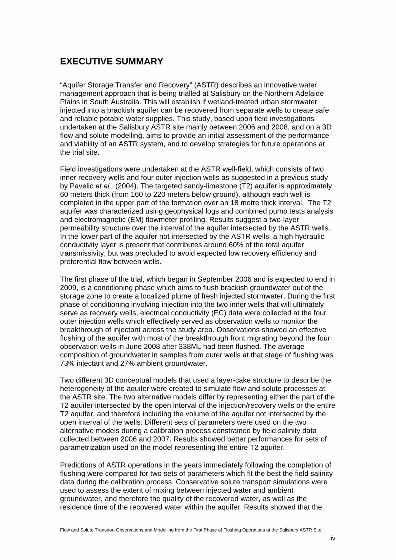
“Aquifer Storage Transfer and Recovery” (ASTR) describes an innovative water management approach that is being trialled at Salisbury on the Northern Adelaide Plains in South Australia. This will establish if wetland-treated urban stormwater injected into a brackish aquifer can be recovered from separate wells to create safe and reliable potable water supplies. This study, based upon field investigations undertaken at the Salisbury ASTR site mainly between 2006 and 2008, and on a 3D flow and solute modelling, aims to provide an initial assessment of the performance and viability of an ASTR system, and to develop strategies for future operations at the trial site. Field investigations were undertaken at the ASTR well-field, which consists of two inner recovery wells and four outer injection wells as suggested in a previous study by Pavelic et al., (2004). The targeted sandy-limestone (T2) aquifer is approximately 60 meters thick (from 160 to 220 meters below ground), although each well is completed in the upper part of the formation over an 18 metre thick interval. The T2 aquifer was characterized using geophysical logs and combined pump tests analysis and electromagnetic (EM) flowmeter profiling. Results suggest a two-layer permeability structure over the interval of the aquifer intersected by the ASTR wells. In the lower part of the aquifer not intersected by the ASTR wells, a high hydraulic conductivity layer is present that contributes around 60% of the total aquifer transmissivity, but was precluded to avoid expected low recovery efficiency and preferential flow between wells. The first phase of the trial, which began in September 2006 and is expected to end in 2009, is a conditioning phase which aims to flush brackish groundwater out of the storage zone to create a localized plume of fresh injected stormwater. During the first phase of conditioning involving injection into the two inner wells that will ultimately serve as recovery wells, electrical conductivity (EC) data were collected at the four outer injection wells which effectively served as observation wells to monitor the breakthrough of injectant across the study area. Observations showed an effective flushing of the aquifer with most of the breakthrough front migrating beyond the four observation wells in June 2008 after 338ML had been flushed. The average composition of groundwater in samples from outer wells at that stage of flushing was 73% injectant and 27% ambient groundwater. Two different 3D conceptual models that used a layer-cake structure to describe the heterogeneity of the aquifer were created to simulate flow and solute processes at the ASTR site. The two alternative models differ by representing either the part of the T2 aquifer intersected by the open interval of the injection/recovery wells or the entire T2 aquifer, and therefore including the volume of the aquifer not intersected by the open interval of the wells. Different sets of parameters were used on the two alternative models during a calibration process constrained by field salinity data collected between 2006 and 2007. Results showed better performances for sets of parametrization used on the model representing the entire T2 aquifer. Predictions of ASTR operations in the years immediately following the completion of flushing were compared for two sets of parameters which fit the best the field salinity data during the calibration process. Conservative solute transport simulations were used to assess the extent of mixing between injected water and ambient groundwater, and therefore the quality of the recovered water, as well as the residence time of the recovered water within the aquifer. Results showed that the

Flow and Solute Transport Observations and Modelling from the First Phase of Flushing Operations at the Salisbury ASTR Site
v
salinity of the recovered water remained largely below 500 mg/L TDS. For one of the alternative sets of parameters, water quality was predicted to remain below 300 mg/L. In all cases the residence time of the injected water exceeded 200 days, which meets the proposed target requirements for inactivation of microbial contaminants and for biodegradation of trace organic contaminants. Both parametrizations were applied to determine the salinity of the recovered water for a 200, 400 and 600 ML injection in the outer wells prior to recovery, to recommend on the procedure of the final stage of the conditioning phase. Both parametrizations predicted that 400 ML was needed in order to recover water of acceptable quality through six annual ongoing cycles in wet, dry or normal years. The additional benefits of 600 ML injection were marginal for all scenarios with both sets of parametrization.
These results support the expected viability of ASTR operations even under stressed (ie. low rainfall) conditions and highlight the potential for a brackish aquifer to be transformed into a storage that has the potential to provide potable supplies. Field investigations are continuing so as to refine and validate the numerical model based on ongoing ASTR operations, with a view to confident use of the model for operational decision making.

Flow and Solute Transport Observations and Modelling from the First Phase of Flushing Operations at the Salisbury ASTR Site
vi
CONTENTS
ACKNOWLEDGEMENTS...........................................................................................iii
EXECUTIVE SUMMARY ............................................................................................iv
CONTENTS ................................................................................................................vi
ACRONYMS .............................................................................................................viii
LIST OF FIGURES ...................................................................................................viii
LIST OF TABLES........................................................................................................x
1 INTRODUCTION....................................................................................................1
2 PREVIOUS WORK AND SITE DESCRIPTION.....................................................1
3 REGIONAL HYDROGEOLOGY ............................................................................3
4 LOCAL AQUIFER CHARACTERIZATION............................................................4
4.1 Characterization Methods ..........................................................................4
4.1.1 Geophysical Logs............................................................................4
4.1.2 Pumping Tests.................................................................................4
4.1.3 EM Flowmeter Profiling...................................................................5
4.2 Aquifer Characterization Results...............................................................5
4.2.1 Vertical Unit Stratification...............................................................5
4.2.2 Aquifer Hydraulic Properties..........................................................6
4.2.3 Integration of Characterization Data..............................................9
5 ASTR FLUSHING OPERATIONS .......................................................................10
5.1 ASTR Well Field.........................................................................................10
5.2 ASTR Flushing Schedule..........................................................................10
6 GROUNDWATER MONITORING........................................................................11
6.1 Materials and Method................................................................................11
6.1.1 Data Collection...............................................................................11
6.1.2 Mixing Fraction ..............................................................................12
6.2 Results and discussion ............................................................................12

Flow and Solute Transport Observations and Modelling from the First Phase of Flushing Operations at the Salisbury ASTR Site
vii
6.2.1 Ambient and Injected Water Quality ............................................12
6.2.2 Solute Breakthrough at Observation Wells.................................13
6.2.3 Evidence of Heterogeneity............................................................14
6.2.4 Comparison of Sampled EC Versus Profiled EC........................17
6.2.5 Intra-Well Flow and Effects on Solute Observations .................17
7 GROUNDWATER MODELLING..........................................................................18
7.1 Numerical Materials and Methods ...........................................................18
7.1.1 Simulation Package.......................................................................18
7.1.2 Development of Conceptual Models............................................18
7.1.3 Model Discretization and Boundary Conditions.........................19
7.1.4 Numerical Methods of Analysis ...................................................21
7.1.5 Calibration Strategy.......................................................................22
7.1.6 Evaluation of Model Performance................................................23
7.2 Numerical Results and Discussion..........................................................24
7.2.1 Evaluation of Model Performance................................................24
7.2.2 Preliminary Sensitivity Analysis ..................................................27
7.2.3 Predictions of Strategies for Progressing Trial ..........................29
8 CONCLUSION .....................................................................................................36
9 RECOMMENDATIONS........................................................................................37
REFERENCES...........................................................................................................38
APPENDIX 1: Overview of 3D Model Simulations of ASTR That Take Heterogeneity into Account, Carried Out in 2005 .................................................40
APPENDIX 2: Input Data for Modelling ..................................................................44
APPENDIX 3: Comparison of Observed and Simulated Drawdown in ASTR Wells During Step-Drawdown Pump Testing of IW1, IW2 and IW4 .....................47

Flow and Solute Transport Observations and Modelling from the First Phase of Flushing Operations at the Salisbury ASTR Site
viii
ACRONYMS
ASR Aquifer Storage and Recovery ASTR Aquifer Storage Transfer and Recovery CSIRO Commonwealth Scientific and Industrial Research Organisation EC Electrical Conductivity RMSE Root-Mean-Square Error TDS Total Dissolved Solids LIST OF FIGURES Figure 1: City of Salisbury water harvesting facilities in the Parafield area, identifying
the location of wells at the ASTR, ASR and GRS sites............................................... 2
Figure 2: Location map for the ASTR well-field showing four injection wells (IW1-
IW4), two recovery wells (RW1-RW2) and three piezometers (P1-P3). ..................... 3
Figure 3: K/Kavg interpreted from EM flowmeter analysis versus depth at RW1,
RW2, IW1 and IW2, showing comparison with average 2-layered K/Kavg profile
(dashed line). .............................................................................................................. 8
Figure 4: K/Kavg interpreted from EM flowmeter analysis versus depth at Greenfield
Railway Station observation well (GRS2). .................................................................. 8
Figure 5: K/Kavg versus depth at ASR observation well (PASR) and Greenfield
Railway Station well (GRS1) between 185 and 200 meters depth. ............................ 9
Figure 6: Time versus cumulative volume of water injected in the aquifer at the
ASTR site during the flushing phase from September 2006 to April 2008, with a
distinction between flow through RW1 and RW2, and time versus flow rates at RW1
and RW2. .................................................................................................................. 11
Figure 7: Time series plot of EC at the outlet-end of the wetland, representative of
the salinity of the injected water in the ASTR system, for 2006 and 2007. ............... 13
Figure 8: Time versus depth-average EC data obtained from down-hole profiles over
the opened intervals at the observation wells IW1, IW2, IW3 and IW4 during the
flushing phase in 2006 & 2007, showing the solute breakthrough of the injectant in
the aquifer. The ASTR operational schedule is also presented. ............................... 14
Figure 9: EC versus depth at observation wells IW1 and IW3 (main transect) during
flushing operation, from March 2007 to April 2008. .................................................. 16
Figure 10: EC versus depth at observation wells IW2 and IW4 (small transect)
during flushing operation, from March 2007 to April 2008. ....................................... 16
Figure 11: Profiled EC versus sampled EC from IW wells on three occasions........ 17
Figure 12: Schematic 3D view of conceptual model CM1 & CM2 showing material
layers......................................................................................................................... 19

Flow and Solute Transport Observations and Modelling from the First Phase of Flushing Operations at the Salisbury ASTR Site
ix
Figure 13: Schematic 3D view of CM2 showing boundary conditions, vertical
numerical layers and a plan view of mesh design with expanded view of near-ASTR
wells zone. ................................................................................................................ 20
Figure 14: Comparison of observed and predicted f versus time at observation wells
IW1, IW2, IW3 and IW4 for models A and B, over 684 days of flushing operations at
the ASTR site (Time from first injection into RW1 and RW2).................................... 25
Figure 15: Comparison of mixing fraction distribution simulated on model A and
model B for the calibration scenario after 684 days. The horizontal scale is about
250 meters while the vertical scale is 50 meters, encompassing the material layers 0
to 5. ........................................................................................................................... 27
Figure 16: Time versus simulated breakthroughs at IW1 [model A] over 684 days of
the flushing period, showing the comparison of three simulations: one taking account
of ASR operations, one taking account of inversed ASR operations and one not
taking account of ASR operations............................................................................. 28
Figure 17: Time since the first day of pumping versus the residence time of the
recovered water within the ground (100 days of injection through RW - recovery
through IW - no storage period - flow rate at 5L/s - model A). .................................. 29
Figure 18: Time versus average simulated salinity concentration at recovery wells
RW1 and RW2 during the conditioning phase of the ASTR trial, for scenarios 1, 2
and 3, for models A and B......................................................................................... 30
Figure 19: Effect of volume of water injected during the first injection period through
IW1, IW2, IW3 and IW4 on recovered water salinity at RW1 and RW2, simulated on
model A and model B................................................................................................ 32
Figure 20: Volume of water recovered versus distribution of residence time in the
aquifer since recovery begun at RW1 and RW2, without storage period between end
of injection at IW wells and recovery......................................................................... 34
Figure 21: Comparison of simulated distribution of the age of water at the end of an
injection period through IW wells (scenario 3a) over the main transect IW1-RW1-
RW2-RW3. The horizontal scale is about 250 meters while the vertical scale is 50
meters, encompassing the material layers 0 to 5...................................................... 35
Figure 22: Parafield ASR injection and recovery schedule from 2006 to 2007.
Positive y-values indicate injection through either 1 or 2 wells, whilst negative values
indicate recovery through either 1 or 2 wells............................................................. 46

Flow and Solute Transport Observations and Modelling from the First Phase of Flushing Operations at the Salisbury ASTR Site
x
LIST OF TABLES
Table 1: Generalized hydrogeological units at ASTR site (modified from AGT (2007)
and Gerges, (2005). .................................................................................................... 6
Table 2: Summary of aquifer properties interpreted from pumping tests (modified
from AGT, 2007 and NGZ, 2005)................................................................................ 6
Table 3: Summary of open well interval [metres bgl] (modified from AGT, 2007). ... 10
Table 4: Summary of ambient groundwater and injected water salinity values........ 13
Table 5: Conceptual Model 1 and 2 parameters and values used during the
calibration process. ................................................................................................... 22
Table 6: Summary of adjusted parameters and changes in RMSE of mixing fraction
during the calibration process constrained by EC data............................................. 24
Table 7: Comparison of salinity [mg/L TDS] over the years 4-6 at recovery wells
RW1 and RW2 for cycle a, b and c, simulated after scenarios 1, 2 and 3, for models
A and B. .................................................................................................................... 33

Flow and Solute Transport Observations and Modelling from the First Phase of Flushing Operations at the Salisbury ASTR Site
1
1 INTRODUCTION “Aquifer Storage Transfer and Recovery” (ASTR) describes a concept that is being trialled at Salisbury on the Northern Adelaide Plains in South Australia. This will establish if wetland-treated urban stormwater injected into a brackish aquifer can be recovered from separate wells to create safe and reliable drinking water supplies (Rinck-Pfeiffer et al. 2005; Swierc et al. 2005, Dillon et al. 2008). Like ‘Aquifer Storage and Recovery’ (ASR) systems that operate throughout the world, ASTR is a method of enhancing subsurface storage which provides an efficient buffer against seasonal variation in water supplies and allows natural treatment to take place within the aquifer. Nevertheless, ASTR differs from ASR systems, which use the same well for both injection and recovery, by using separate wells, that should provide a longer and more uniform residence time within the aquifer to ensure more reliable inactivation of pathogen and biodegradation of trace organics. This study, based on field investigations undertaken at the Parafield ASTR site between 2006 and 2008, and on 3D flow and solute transport modelling, aims to provide an initial assessment of the performance and viability of the ASTR system. It also provides an opportunity to evaluate the feasibility of transforming a brackish aquifer into a potable water storage. After detailing the broad aims of the ASTR project, the present report documents the results of investigations to characterize the targeted aquifer, a pre-requisite to any groundwater project to understand the heterogeneous distribution of hydraulic properties of the porous media. Next, the report outlines the ASTR flushing operations taking place during the conditioning phase of the trial, which began in 2006 and is expected to finish in 2009, and describes the breakthrough of the fresh water plume at observation wells induced by ASTR operations within the brackish aquifer. Finally, the report provides details of 3D flow and solute transport modelling which simulates actual and proposed ASTR operations using two alternative conceptual models based on aquifer characterization and solute breakthrough data currently available. Recommendations are offered on the way the final phase of aquifer conditioning should proceed to ensure that salinity and residence time criteria are met over the first six years of regular ASTR operations. 2 PREVIOUS WORK AND SITE DESCRIPTION
A previous study by Pavelic et al., (2004) developed a 2D FEFLOW groundwater model based on limited data for aquifer characterisation and whose accuracy was validated by a semi-analytical method based on Theis equations. This initial model was used to establish the optimal well-field design. The operation was considered to have two key constraints. Firstly, a residence time of injected water within the aquifer greater than 200 days was required to ensure inactivation of pathogens. Secondly, recovered water, which is a mixture of native groundwater and injected water, should contain no more than 10% of native groundwater to achieve the target quality of less than 300 mg/L Total Dissolved Solids (TDS). The results showed that the best configuration which met the required criteria was a six-well system of four outer injection wells and two inner recovery wells all equi-spaced with an inter-well separation distance of 75 m. However, subsequent to the Pavelic et al., (2004) study following the collection of local aquifer hydraulic conductivity data from a newly constructed well and two existing wells led to a revision of the conceptual model of the aquifer. This indicated that a reduction in the inter-well spacing from 75 m to 50 m
Flow and Solute Transport Observations and Modelling from the First Phase of Flushing Operations at the Salisbury ASTR Site
2
was needed, and that partially-penetrating wells should be constructed to preclude the low recovery efficiency and preferential flow that would invariably occur if the lower interval of the target aquifer with high hydraulic conductivity was also intercepted. An inventory of the model simulations and results undertaken between the Pavelic et al., (2004) study and this study are summarized in Appendix 1, along with the rational for changing the location of the well-field from the area immediately adjacent to the Greenfields Railway Station, as was initially intended, to the Parafield Gardens Oval.
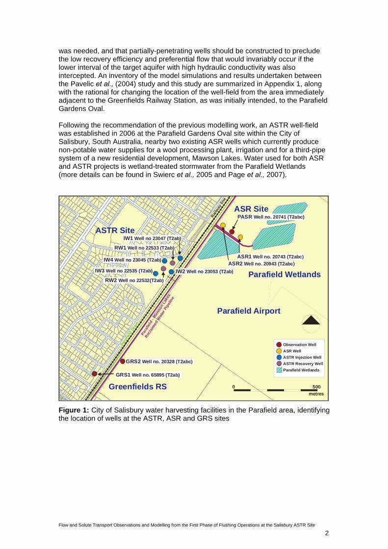
Following the recommendation of the previous modelling work, an ASTR well-field was established in 2006 at the Parafield Gardens Oval site within the City of Salisbury, South Australia, nearby two existing ASR wells which currently produce non-potable water supplies for a wool processing plant, irrigation and for a third-pipe system of a new residential development, Mawson Lakes. Water used for both ASR and ASTR projects is wetland-treated stormwater from the Parafield Wetlands (more details can be found in Swierc et al., 2005 and Page et al., 2007).
Pa
rafie
ld -
Mawso
n La
kes
Recl
aimed
Wat
er P
ipeli
ne
Parafield Wetlands
ASR1 Well no. 20743 (T2abc)
GRS1 Well no. 65895 (T2ab)
PASR Well no. 20741 (T2abc)
ASR2 Well no. 20943 (T2abc)
GRS2 Well no. 20328 (T2abc)
ASTR Site IW1 Well no 23047 (T2ab)
IW3 Well no 22535 (T2ab)
RW1 Well no 22533 (T2ab)
IW4 Well no 23045 (T2ab)
RW2 Well no 22532(T2ab)
Greenfields RS
Observation WellASR WellASTR Injection WellASTR Recovery WellParafield Wetlands
Para
field
Dra
in
Rail
way lin
e
500 0 metres
ASR Site
IW2 Well no 23053 (T2ab)
Parafield Airport
Figure 1: City of Salisbury water harvesting facilities in the Parafield area, identifying the location of wells at the ASTR, ASR and GRS sites

Flow and Solute Transport Observations and Modelling from the First Phase of Flushing Operations at the Salisbury ASTR Site
3
IW3 Well no 22535 (T2ab)
RW2 Well no 22532 (T2ab)
Residential
P1 (T2ab)P2 (T2c)
P3 (T2ab)
Residential
ASTR Site
PiezometerASTR Injection WellASTR Recovery Well
Extraction Injection
IW4 Well no 23045 (T2ab)
50 0 metres
IW1 Well no 23047 (T2ab)
IW2 Well no 23053 (T2ab)
RW1 Well no 22533 (T2ab)
Parafield Airport
Figure 2: Location map for the ASTR well-field showing four injection wells (IW1-IW4), two recovery wells (RW1-RW2) and three piezometers (P1-P3).
3 REGIONAL HYDROGEOLOGY The ASTR trial site is located on the Northern Adelaide Plains (NAP) in South Australia. The site is underlain by Quaternary and Tertiary sediments lying on a Precambrian basement. The Quaternary deposits contain four aquifers, and the Tertiary sediments can contain up to four aquifers called T1, T2, T3 and T4 in order of increasing depth. The first and second Tertiary aquifers are the most intensively used aquifers, mainly for irrigation purposes (Zulfic, 2002). Almost flat lying, T1 and T2 constitute the Port Willunga Formation, and are separated by a confining bed, the Munno Para Clay Member. The ASTR trial targeted the T2 aquifer which represents the lower part of the Port Willunga Formation which consists of well-cemented limestone with sand and sandstones with an average thickness of 60 meters (AGT, 2007). The lithological and salinity stratifications suggest that the T2 aquifer can be divided into three units called T2a, T2b and T2c in order of increasing depth (Gerges, 1999).
The ambient regional groundwater flow in the T2 aquifer beneath the study site is approximately from east to west with a regional hydraulic gradient of 0.0015 without significant seasonal variations (Pavelic et al., 2004). A stronger local gradient occurs due to the Parafield ASR operations situated around 300m N-NE of the study site (Figure 1). The two ASR wells intersect the entire T2 aquifer. The direction of this local gradient varies as a function of the ASR operations. During recovery periods at

Flow and Solute Transport Observations and Modelling from the First Phase of Flushing Operations at the Salisbury ASTR Site
4
the ASR site, the flow is towards the north-east while during injection it is towards the south-west. Values of this local gradient vary in response to ASR and ASTR operations, and can be as high as 0.03 (as calculated from the head data from model B presented below during times of injection at the ASR site and no activity at the ASTR site).
4 LOCAL AQUIFER CHARACTERIZATION Various hydrogeological methods were used to determine the distribution of hydraulic properties of the target aquifer T2 including stratigraphic logs, geophysical logs, electromagnetic (EM) flowmeter profiling and aquifer pumping test analyses. Field measurements were undertaken at nine wells, of which six are partially penetrating wells with open intervals in T2a and T2b (ASTR wells IW1 (6628-23047), IW2 (6628-23053), IW3 (6628-22533), IW4 (6628-23045), RW1 (6628-22532) and RW2 (6628-22535) at Parafield Oval Garden) (Figure 2), and three are fully penetrating wells in T2 (Greenfield Railway Station well (GRS1 (6628-65895) and GRS2 (6628-20328)) and the Parafield ASR (PASR) observation well (6628-20741)). In this report the two inner wells of the ASTR well-field will be referred to as ‘recovery wells’ (RW) and the four outer wells as ‘injection wells’ (IW).
4.1 Characterization Methods
4.1.1 Geophysical Logs
Conventional geophysics logs, including gamma, neutron, caliper, density, point resistivity, self potential, medium induction and deep induction were run prior to installation of the casing to assess the lithological stratigraphy of the targeted aquifer.
4.1.2 Pumping Tests
Depth-averaged transmissivity and storage coefficient were interpreted from the drawdown data from pump tests conducted in partially and fully penetrating wells across the field site. Depth averaged transmissivity was derived from a constant discharge test, upon the establishment of a quasi-steady state, using the equation:
0.183 QTs
=Δ
Equation 1
where T is the transmissivity (m2/d), Q the discharge rate (m3/d) and sΔ the drawdown per log cycle (m) (Cooper and Jacob, 1946). Analysis of the observations from a transient pump test was used to determine storage coefficient, using the equation:
2
.2.25 r
T toS = Equation 2
where S is the storage coefficient, T is the transmissivity (m2/d), to the time at zero drawdown and r the distance from the pumping well (m).

Flow and Solute Transport Observations and Modelling from the First Phase of Flushing Operations at the Salisbury ASTR Site
5
Constant rate discharge and step drawdown tests were carried out at the ASTR site in 2006 and 2007 (AGT, 2007). 5-hour step drawdown tests were conducted on RW1, RW2 and IW3 at 3, 6 and 9L/s for 100 minutes during each step in June 2006. During the same month, constant discharge tests were carried out for one day on RW1 and IW3 at a discharge rate of 9L/s. In February 2007, 8-hour step drawdown tests were conducted on IW1, IW2 and IW4 at the same discharge rates but for 280 minutes during the last step. Step drawdown tests were single-well tests while the constant discharge tests used other RW and IW wells as observation wells.
4.1.3 EM Flowmeter Profiling
To asses the hydrostratigraphy of the targeted aquifer, the vertical distributions of relative hydraulic conductivity were estimated from borehole EM flowmeter logging (Molz et al., 1989, Molz et al., 1994). Field data obtained from the flowmeter device were the ambient flow velocity profile and the induced flow velocity profile measured at same depths determined from caliper logs. The so-called ‘induced flow’ is the flow resulting from pumping the well at a constant rate once steady-state was reached. Flow rates used range from 15 to 20 L/min. A net induced flow can be calculated by subtracting the ambient flow value from the induced flow value. The difference between net induced flows at two successive depths yields the net flow entering the well between the measured depths. Then, assuming that the flow in the aquifer is horizontal, the amount of water entering the well is proportional to the hydraulic conductivity of any layer. According to Molz et al, (1989), the relative hydraulic conductivity (K/Kavg) for each interval i could be derived from:
i i
avg p i
Q bKK Q b
=Σ
Equation 3
where Qi and bi are the net flow contribution and thickness of the layer, Qp is the spumping rate and ibΣ the total depth. Relative distributions of hydraulic conductivity can be interpreted as absolute values by combining EM flowmeter profiles and pumping test-derived data (Güven et al., 1992). Assuming that the pump test derived values of hydraulic conductivity are a reasonable approximation of Kavg, the relative data (K/Kavg) for each well were converted to numerical values by using the conductivity obtained from the pump test analysis.
4.2 Aquifer Characterization Results
4.2.1 Vertical Unit Stratification
Lithological statigraphy of the targeted aquifer was interpreted using geophysical and lithological logs. Comparison of hydrogeological sequences at the ASTR site and nearby Greenfield Railway Station site showed a homogeneous distribution on a broad scale. Intervals over which the various lithological units were intersected at the ASTR and Greenfield Railway Station are described in Table 1. The thickness of aquifer T2 is 60 meters, from 160 to 220 meters depth. It is divided into three sub-aquifers T2a, b and c, with thicknesses of 12, 15 and 33 meters respectively (AGT, 2007).

Flow and Solute Transport Observations and Modelling from the First Phase of Flushing Operations at the Salisbury ASTR Site
6
Table 1: Generalized hydrogeological units at ASTR site (modified from AGT (2007) and Gerges, (2005). Interval [m] Lithology Aquifer Statigraphic name
Overlying aquifers
152.5 - 160 Clay Confining bed Munno Para Clay 160 - 172
Limestone (grey to white)
moderately cemented
T2a unit
172 - 187
Limestone (grey to yellow) well
cemented interbedded with sand/silt
T2b unit
187 - 220
Limestone, sand highly fossilifereous
T2c unit
Lower Port Willunga Formation
220 - 222 Confining bed Ruwarung member
4.2.2 Aquifer Hydraulic Properties Depth-averaged transmissivity and storage coefficient
Analysis of pump tests yields depth-averaged measures of transmissivity, T and storage coefficient, S over the open well intervals. Depth-averaged transmissivities were interpreted to range from 188 to 203 m2/d in fully penetrating wells, while a mean value of 46 m2/d was derived from tests at ASTR wells encompassing 18 meters depth in T2a and T2b (Gerges, 2005; AGT, 2007). Relatively small differences in T values derived from tests at ASTR wells IW1, IW2, IW3, IW4, RW1 and RW2 suggest low lateral heterogeneity, with T ranging from 38 at IW2 to 53 m2/d at IW3 and RW1 (AGT, 2007) as shown in Table 2. Nevertheless, no clear spatial pattern can be interpreted from the different transmissivities. Average storage coefficient derived from transient pump test at partially-penetrating wells across the study site is 2.6x10⁻⁴ (AGT, 2007). Table 2: Summary of aquifer properties interpreted from pumping tests (modified from AGT, 2007 and Gerges, 2005). Parameters Aquifer Wells Average value
IW1 IW2 IW3 IW4 RW1 RW2 T2a,b
45 38 53 41 53 47
46
GRS1 GRS2 T [m2/d]
T2 188 203
195
IW3 RW2 S [ - ]
T2a,b 1.8 to 2.8x10⁻⁴ 1.9 to 2.7 x10⁻⁴
2.6x10⁻⁴
Flow and Solute Transport Observations and Modelling from the First Phase of Flushing Operations at the Salisbury ASTR Site
7
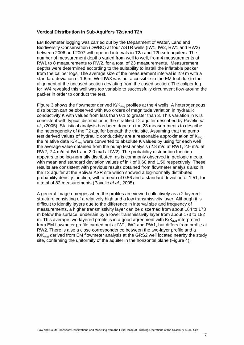
Vertical Distribution in Sub-Aquifers T2a and T2b EM flowmeter logging was carried out by the Department of Water, Land and Biodiversity Conservation (DWBC) at four ASTR wells (IW1, IW2, RW1 and RW2) between 2006 and 2007 with opened intervals in T2a and T2b sub-aquifers. The number of measurement depths varied from well to well, from 4 measurements at RW1 to 8 measurements to RW2, for a total of 23 measurements. Measurement depths were determined according to the suitability to install the inflatable packer from the caliper logs. The average size of the measurement interval is 2.9 m with a standard deviation of 1.6 m. Well IW3 was not accessible to the EM tool due to the alignment of the uncased section deviating from the cased section. The caliper log for IW4 revealed this well was too variable to successfully circumvent flow around the packer in order to conduct the test. Figure 3 shows the flowmeter derived K/Kavg profiles at the 4 wells. A heterogeneous distribution can be observed with two orders of magnitude variation in hydraulic conductivity K with values from less than 0.1 to greater than 3. This variation in K is consistent with typical distribution in the stratified T2 aquifer described by Pavelic et al., (2005). Statistical analysis has been done on the 23 measurements to describe the heterogeneity of the T2 aquifer beneath the trial site. Assuming that the pump test derived values of hydraulic conductivity are a reasonable approximation of Kavg, the relative data K/Kavg were converted to absolute K values by using for each well the average value obtained from the pump test analysis (2.8 m/d at RW1, 2.9 m/d at RW2, 2.4 m/d at IW1 and 2.0 m/d at IW2). The probability distribution function appears to be log-normally distributed, as is commonly observed in geologic media, with mean and standard deviation values of lnK of 0.60 and 1.50 respectively. These results are consistent with previous results obtained from flowmeter analysis also in the T2 aquifer at the Bolivar ASR site which showed a log-normally distributed probability density function, with a mean of 0.56 and a standard deviation of 1.51, for a total of 82 measurements (Pavelic et al., 2005). A general image emerges when the profiles are viewed collectively as a 2 layered-structure consisting of a relatively high and a low transmissivity layer. Although it is difficult to identify layers due to the difference in interval size and frequency of measurements, a higher transmissivity layer can be discerned from about 164 to 173 m below the surface, underlain by a lower transmissivity layer from about 173 to 182 m. This average two-layered profile is in a good agreement with K/Kavg interpreted from EM flowmeter profile carried out at IW1, IW2 and RW1, but differs from profile at RW2. There is also a close correspondence between the two-layer profile and a K/Kavg derived from EM flowmeter analysis at the GRS2 well located nearby the study site, confirming the uniformity of the aquifer in the horizontal plane (Figure 4).
Flow and Solute Transport Observations and Modelling from the First Phase of Flushing Operations at the Salisbury ASTR Site
8
160
170
180
190
0 1 2 3 4
K/Kavg
Dep
th b
gs (m
)
average profileK/Kavg
IW2
160
170
180
190
0 1 2 3 4K/Kavg
Dep
th b
gs (m
)
average profileK/Kavg
IW1
160
170
180
190
0 1 2 3 4K/Kavg
Dep
th b
gs (m
)
average profileK/Kavg
RW1
160
170
180
190
0 1 2 3 4K/Kavg
Dep
th b
gs (m
)
average profileK/Kave
RW2
Figure 3: K/Kavg interpreted from EM flowmeter analysis versus depth at RW1, RW2, IW1 and IW2, showing comparison with average 2-layered K/Kavg profile (dashed line).
160
170
180
190
0 1 2 3 4K/Kavg
Dep
th b
gs (m
)
K/KavgGRS2
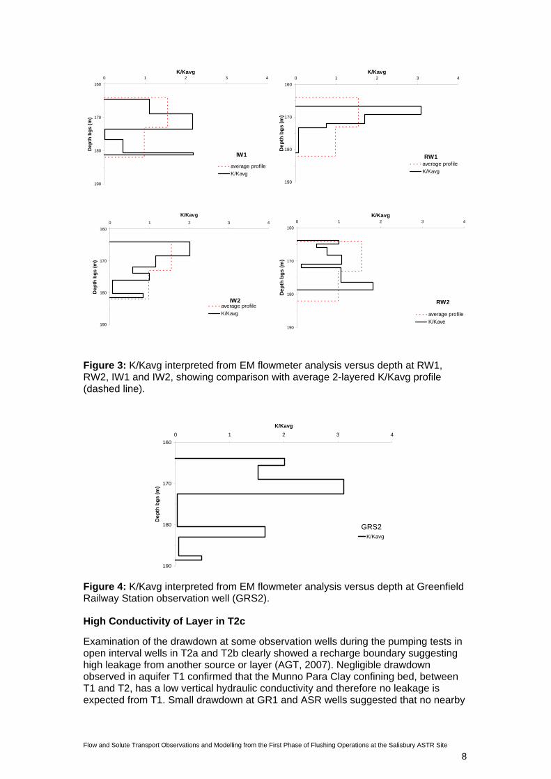
Figure 4: K/Kavg interpreted from EM flowmeter analysis versus depth at Greenfield Railway Station observation well (GRS2).
High Conductivity of Layer in T2c
Examination of the drawdown at some observation wells during the pumping tests in open interval wells in T2a and T2b clearly showed a recharge boundary suggesting high leakage from another source or layer (AGT, 2007). Negligible drawdown observed in aquifer T1 confirmed that the Munno Para Clay confining bed, between T1 and T2, has a low vertical hydraulic conductivity and therefore no leakage is expected from T1. Small drawdown at GR1 and ASR wells suggested that no nearby

Flow and Solute Transport Observations and Modelling from the First Phase of Flushing Operations at the Salisbury ASTR Site
9
source affects the trial area, and that the observed leakage is from the underlying T2c unit. This interpretation has been reinforced by K/Kavg profiles interpreted from EM flowmeter logs carried out in 2005 in open holes from 160 to 200 meters depth at GRS1 and ASR wells. K/Kavg profiles showed a very high conductivity layer from about 195 to 200 meters depth, with a thickness of several meters, with K/Kavg values of 15 (GRS well) and 21 (PASR well) as shown in Figure 5. Using the average value of K= 3.3 m/d derived from pumping test over T2 (Gerges, 2005), the relative data K/ Kavg yield absolute values of hydraulic conductivity of 48 to 66 m/d in the conductive layer between about 195 to 200 meters depth, and 2 m/d between 185 and 195 meters depth. This clearly attests to the presence of a high conductivity layer in T2c, which is likely to be responsible of the variation of the drawdown observed during the pumping test.
185
195
0 5 10 15 20 25K/Kavg
Dep
th b
gs (m
)
ASR observation wellGRS well
Figure 5: K/Kavg versus depth at ASR observation well (PASR) and Greenfield Railway Station well (GRS1) between 185 and 200 meters depth.
4.2.3 Integration of Characterization Data
Not surprisingly, given the sedimentary nature of the aquifer, interpretation of the characterization data yields a conceptual model of the targeted T2 aquifer that has a layer-cake structure. Lithological and geophysical logs, confirmed by horizontal distribution of hydraulic properties derived from pump test analysis and EM flowmeter analysis, showed that the aquifer is far less heterogeneous in the horizontal plane than in the vertical plane. The absolute hydraulic conductivities interpreted from pumping test analysis and EM flowmeter analysis revealed a high degree of heterogeneity between layers within the aquifer. Nevertheless, the interpretation of the flowmeter data, supported by lithological logs, suggests a conceptual model that is a two-layer model within the T2a and b sub-aquifers, with a higher conductivity layer above a lower conductivity layer. Further data from EM flowmeter analysis at nearby wells clearly showed a thin very high conductivity layer at about 195 to 200 meters depths within the T2c sub-aquifer.

Flow and Solute Transport Observations and Modelling from the First Phase of Flushing Operations at the Salisbury ASTR Site
10
5 ASTR FLUSHING OPERATIONS
5.1 ASTR Well Field
As described previously, the Parafield ASTR system is a six-well system progressively drilled between 2006 and 2007. RW1, RW2 and IW3 were drilled in May 2006 while IW1, IW2 and IW4 were drilled in January 2007. The ASTR wells were completed as ‘open hole’ in sub-aquifers T2a and T2b with depth intervals averaging 165 to 182 meters (Table 3). Preferential flow would have occurred if the high transmissivity layer in the T2c sub-aquifer was intercepted. Previous modelling work found that salinity could not be sustained at less than 300 mg/L if this layer was intercepted by the ASTR wells (Appendix 1). The vertical separation between the base of the IW and RW wells and the high hydraulic conductivity layer which appears on the EM flowmeter analysis ranged from 11 to 15 meters. A summary of open intervals of each well is presented in Table 3. All wells were cased using 200 mm PVC casing to the depth of the top of the open hole, and then successfully pressure cemented (AGT, 2007). Airlifting was carried out at all wells for approximately four hours and each well produced a small amount of sand and estimated well yields are approximately 10 L/s. Table 3: Summary of open well interval [metres bgl] (modified from AGT, 2007).
Well IW1 IW2 IW3 IW4 RW1 RW2 Open interval [m bgl] 168-183 164-184 168-183 164-184 165-182 164-180
5.2 ASTR Flushing Schedule
The first phase of the ASTR trial, which began in September 2006, is a conditioning phase which aims to flush brackish groundwater out of the storage zone to ensure that the efficiency of the system can be sustained during recovery when the ASTR trial advances to the normal operating mode. To efficiently displace ambient groundwater out of the trial area, fresh water was injected through inner ‘recovery wells’ RW1 and RW2. Outer ‘injection wells’ were used as observation wells to monitor the breakthrough of the injectant.
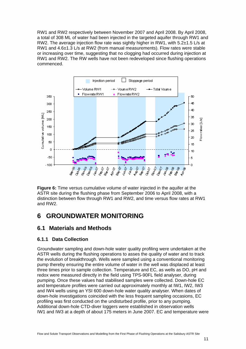
A detailed schedule of the injection, cumulative volume injected into the aquifer and flow rates at RW1 and RW2 are presented on Figure 6. Flow rates and cumulative volume were monitored from September 2006 using manual measurements collected from a Siemens battery powered EM flowmeter (MAG8000). From July 2007, Siemens data compressors (FAU:DC02) were connected to both wells to collect flow rates at ten minutes intervals. Logged data and manual measurements during site visits are closely matched in all cases, except for the flow rate logger at RW2 which malfunctioned after 1 month. A first injection period was carried out from September 2006 to January 2007 involving 43 ML injected through RW1 and 35 ML injected through RW2, for a total of 78 ML stored in the aquifer. A second injection phase occurred from May 2007 to October 2007, after four months of stoppage period, involving 140 ML injected through RW1 and 120 ML injected through RW2. A third injection period occurred after one and a half months of stoppage involved 72 ML and 50 ML injected through
Flow and Solute Transport Observations and Modelling from the First Phase of Flushing Operations at the Salisbury ASTR Site
11
RW1 and RW2 respectively between November 2007 and April 2008. By April 2008, a total of 308 ML of water had been injected in the targeted aquifer through RW1 and RW2. The average injection flow rate was sightly higher in RW1, with 5.2±1.5 L/s at RW1 and 4.6±1.3 L/s at RW2 (from manual measurements). Flow rates were stable or increasing over time, suggesting that no clogging had occurred during injection at RW1 and RW2. The RW wells have not been redeveloped since flushing operations commenced.
Figure 6: Time versus cumulative volume of water injected in the aquifer at the ASTR site during the flushing phase from September 2006 to April 2008, with a distinction between flow through RW1 and RW2, and time versus flow rates at RW1 and RW2.
6 GROUNDWATER MONITORING
6.1 Materials and Methods
6.1.1 Data Collection
Groundwater sampling and down-hole water quality profiling were undertaken at the ASTR wells during the flushing operations to asses the quality of water and to track the evolution of breakthrough. Wells were sampled using a conventional monitoring pump thereby ensuring the entire volume of water in the well was displaced at least three times prior to sample collection. Temperature and EC, as wells as DO, pH and redox were measured directly in the field using TPS-90FL field analyser, during pumping. Once these values had stabilised samples were collected. Down-hole EC and temperature profiles were carried out approximately monthly at IW1, IW2, IW3 and IW4 wells using an YSI 600 down-hole water quality analyser. When dates of down-hole investigations coincided with the less frequent sampling occasions, EC profiling was first conducted on the undisturbed profile, prior to any pumping. Additional down-hole CTD-diver loggers were established in observation wells IW1 and IW3 at a depth of about 175 meters in June 2007. EC and temperature were
Flow and Solute Transport Observations and Modelling from the First Phase of Flushing Operations at the Salisbury ASTR Site
12
monitored continuously in the wetland from September 2006. An Odyssey EC/Temperature logger was used in the Parafield wetland from September 2006 to August 2007, and then switched to a CTD-diver logger. Both of the wetlands loggers took measurements every 30 minutes at a depth of about 30 cm from the base of the pond, near the wetland inlet and outlet. Total Dissolved Solids (TDS) concentration derived from field EC data was used as a salinity indicator. A linear regression equation was used with reasonable confidence to demonstrate the relationships between these variables. During examination of the field data, temperature was highly variable over short intervals and did not appear easily interpretable to assess the movement and mixing of the injected water within the aquifer. Therefore, in the following discussion, breakthroughs of injectant are described using salinity data, either expressed as TDS or EC values.
6.1.2 Mixing Fraction
Any conservative solute, for which the concentration in the injected water differs sufficiently from the concentration in the native groundwater, can be used as a tracer to quantify the movement and the mixing of the injected water within the aquifer. A mixing fraction, representing the proportion of the injectant in a sampled mixture, can be estimated at any time from the following simple mass balance Equation 4:
ambinj
ambmix
CCCtC
tf
)()(
−−
= Equation 4
where Cinj is the concentration in conservative solute in injected water, Camb is the conservative solute concentration in the native groundwater and C(t)mix is the conservative solute concentration in the mixture at any particular time. Mixing fraction can be expressed in terms of an absolute value, from 0 to 1, or in percentage terms (where a value of 1 corresponds to 100%). In this study, salinity was chosen as tracer because it behaves relatively conservatively in the system; the pronounced distinction between ambient and injected concentrations; and the abundance of data. In the following discussion, mixing fraction will be calculated using average EC data from ambient groundwater and injected water.
6.2 Results and discussion
6.2.1 Ambient and Injected Water Quality
Ambient groundwater salinity was derived from pumped EC data collected at RW1, RW2 and IW3 after drilling in May 2006. Values were 3,650, 3,630 and 3,620 µS/cm respectively, yielding a mean value of 3,633 µS/cm (Table 4). Injected water salinity was monitored from October 2006 to January 2008 with an EC logger located at the outlet of the wetland and by sampled EC collected at the outlet of the wetland or at injection wells RW1 and RW2. Sampled EC values ranged from 167 to 352 µS/cm with an average value of 253 µS/cm and a standard deviation of 51 µS/cm. These observations are in good agreement with logged EC from the wetland which averaged 244 µS/cm with a standard deviation of 58 µS/cm, from measurements taken every 30 minutes from November 2006 to August 2007. In the following

Flow and Solute Transport Observations and Modelling from the First Phase of Flushing Operations at the Salisbury ASTR Site
13
discussion, mixing fraction will be calculated using ECinj = 250 µS/cm and ECamb = 3,633 µS/cm. Table 4: Summary of ambient groundwater and injected water salinity values.
Average EC [µS/cm]
Standard deviation [µS/cm]
Number of measurements
Ambient groundwater
3,633 15 3 (in May 2006)
Sample 253 51 20 (from 10/06 to 01/08)
Injected water Logger 244 58 every 30 minutes
(from 11/06 to 08/07) Temporal variations in salinity can be observed on the EC log from the outlet of the wetland (Figure 7). Salinity tends to be lower in winter when more stormwater is available, than in summer when there is less flow through the wetland, allowing evaporative concentration due to the shallow water table and increasing residence time. Moreover, although the ASTR system is designed to inject wetland-treated stormwater into the aquifer, marginally more saline water from the nearby Parafield ASR system was used to flush the brackish aquifer when insufficient stormwater was available during dry periods. Since the water recovered from the Parafield ASR system was first cycled through the wetland before being injected at the ASTR site, assessment of the salinity of the injectant can be made from measurements made at the outlet of the wetland.
0
100
200
300
400
500
1/09/2006 10/12/2006 20/03/2007 28/06/2007 6/10/2007
Time
EC [u
S/cm
]
Field/ Lab EC
Log Ec
Figure 7: Time series plot of EC at the outlet-end of the wetland, representative of the salinity of the injected water in the ASTR system, for 2006 and 2007.
6.2.2 Solute Breakthrough at Observation Wells
EC data were recorded on approximately a monthly basis by profiling at observation wells IW1, IW2, IW3 and IW4 to quantitatively trace the presence of the injectant within the aquifer during the flushing operations. Depth-averaged values were derived from EC profiles using all data from the open well interval (Figure 8). Partial breakthroughs of the injected water were observed at all observation wells with the first significant drop in salinity evident from December 2006, 104 days after the beginning of water injection through RW1 and RW2 when 70 ML had been injected.
Flow and Solute Transport Observations and Modelling from the First Phase of Flushing Operations at the Salisbury ASTR Site
14
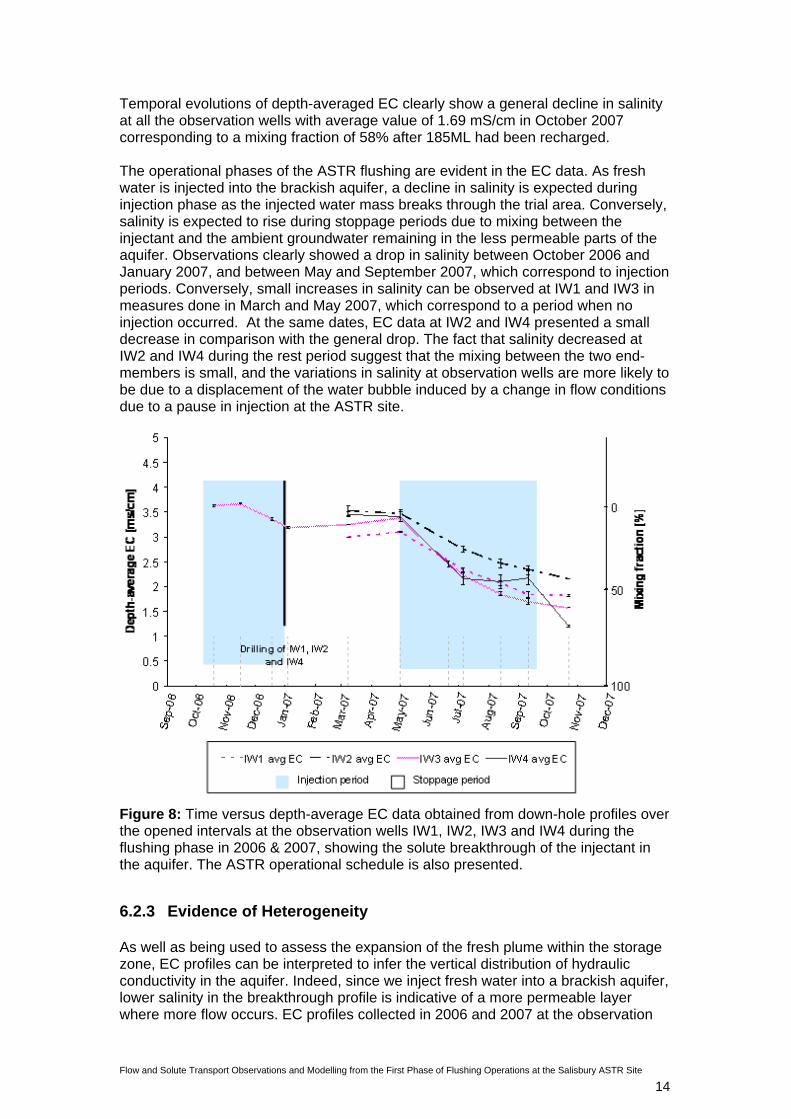
Temporal evolutions of depth-averaged EC clearly show a general decline in salinity at all the observation wells with average value of 1.69 mS/cm in October 2007 corresponding to a mixing fraction of 58% after 185ML had been recharged. The operational phases of the ASTR flushing are evident in the EC data. As fresh water is injected into the brackish aquifer, a decline in salinity is expected during injection phase as the injected water mass breaks through the trial area. Conversely, salinity is expected to rise during stoppage periods due to mixing between the injectant and the ambient groundwater remaining in the less permeable parts of the aquifer. Observations clearly showed a drop in salinity between October 2006 and January 2007, and between May and September 2007, which correspond to injection periods. Conversely, small increases in salinity can be observed at IW1 and IW3 in measures done in March and May 2007, which correspond to a period when no injection occurred. At the same dates, EC data at IW2 and IW4 presented a small decrease in comparison with the general drop. The fact that salinity decreased at IW2 and IW4 during the rest period suggest that the mixing between the two end-members is small, and the variations in salinity at observation wells are more likely to be due to a displacement of the water bubble induced by a change in flow conditions due to a pause in injection at the ASTR site.
Figure 8: Time versus depth-average EC data obtained from down-hole profiles over the opened intervals at the observation wells IW1, IW2, IW3 and IW4 during the flushing phase in 2006 & 2007, showing the solute breakthrough of the injectant in the aquifer. The ASTR operational schedule is also presented.
6.2.3 Evidence of Heterogeneity As well as being used to assess the expansion of the fresh plume within the storage zone, EC profiles can be interpreted to infer the vertical distribution of hydraulic conductivity in the aquifer. Indeed, since we inject fresh water into a brackish aquifer, lower salinity in the breakthrough profile is indicative of a more permeable layer where more flow occurs. EC profiles collected in 2006 and 2007 at the observation

Flow and Solute Transport Observations and Modelling from the First Phase of Flushing Operations at the Salisbury ASTR Site
15
wells presented variations in the pattern of breakthrough, more likely due to the different flow conditions induced by injection at RW1 and RW2 (Figure 9 and Figure 10). Profiles carried out during injection periods at RW1 and RW2 presented heterogeneous breakthrough while profiles carried out when no ASTR operations occurred were more uniform suggesting vertical mixing over the open well interval. Profiles collected at IW1 and IW3 during injection at RW1 and RW2 showed a clear preferential flow path from with a minimum in salinity between about 168 to 178 meters depth (Figure 9). Profiles collected at the same dates at IW2 and IW4 suggested that more flow occurred between about 170 metres depth and the bottom of the wells (Figure 10). For all of the profiles carried out in July, August and September 2007 when injection occurred on ASTR site, the bottom of the observation well appeared to be fresher than the upper part of the opened interval. Superposition of vertical salinity profile and relative hydraulic conductivity derived from EM flowmeter analysis carried out during injection periods showed a good correspondence in the vertical distribution of hydraulic conductivities at IW1 but not at IW2. When no injection occurred at the trial site, observations wells IW2 and IW4 presented a step-like increase in salinity during profiling done in March and May 2007 at a depth corresponding with the flowmeter-derived conductive layers. In the October 2007 profiles when no ASTR operations occurred, a homogeneous profile in salinity tended to appear at all wells. Finally, the distribution in salinity over the open interval of the well showed evidence of heterogeneity.

Flow and Solute Transport Observations and Modelling from the First Phase of Flushing Operations at the Salisbury ASTR Site 16
160
165
170
175
180
0 0.5 1 1.5 2 2.5 3 3.5 4
IW1 - EC [ms/cm]
Dep
th [m
]
8/03/20071/05/20075/07/200713/08/200711/09/200723/10/20078/04/2008
160
165
170
175
180
0 1 2 3 4
IW3 - EC [ms/cm]
Dep
th T
OC
[m]
19/10/2006
16/11/2006
19/12/2006
4/01/2007
8/03/2007
1/05/2007
20/06/2007
5/07/2007
13/08/2007
11/09/2007
23/10/2007
8/04/2008
Figure 9: EC versus depth at observation wells IW1 and IW3 (main transect) during flushing operation, from March 2007 to April 2008.
IW2 - EC [mS/cm]
160
165
170
175
180
0 0.5 1 1.5 2 2.5 3 3.5 4
Dep
th [m
] 8/03/20071/05/20075/07/200713/08/200711/09/200723/10/2007
IW4 - EC [mS/cm]
160
165
170
175
180
0 1 2 3 4
Dep
th [m
]
8/03/20071/05/20075/07/200713/08/200711/09/200723/10/20078/04/2008
Figure 10: EC versus depth at observation wells IW2 and IW4 (small transect) during flushing operation, from March 2007 to April 2008.

Flow and Solute Transport Observations and Modelling from the First Phase of Flushing Operations at the Salisbury ASTR Site
17
6.2.4 Comparison of Sampled EC versus Profiled EC
EC data were collected using down-hole profiling on approximately a monthly basis, but some coincident sampling on three occasions allowed assessment of EC in pumped samples. Comparison of down-hole profiled and sampled EC data collected at the observation wells at periods when injection occurred at RW wells is presented in Figure 11. It appeared that sampled and profiled EC are similar and quite well correlated at wells IW1 and IW3, and less correlated at IW2 and IW4. Data collected in July 2007 at IW1 and IW3 at the highest salinity concentrations showed that sampled EC were lower than profiled EC by up to 0.6 mS/cm at IW1. Conversely, in September 2007, sampled EC at the same wells appeared to underestimate the breakthrough of fresh water.
At wells IW2 and IW4, comparison of data collected in September 2007 showed a large underestimation of salinity from sampled EC compared to profiled EC by up to 1 mS/cm at IW4. Not surprisingly, the more the fresh plume breaks through the observation zone, the more sampled EC underestimates the profiled EC. Indeed, when pumping occurred, a greater proportion of flow comes from the more permeable layer. Thus as more of the breakthrough front passes the IW wells, the mean of the EC profile measured within the well deviates from the flux-averaged EC of the adjacent groundwater measured during sampling. Therefore, the underestimation of sampled EC relative to the profiled EC suggested that the more permeable layer contains fresher water, assessing the breakthrough of the injectant within a heterogeneous aquifer. These contrasts between flux-averaged and volume averaged concentrations suggest that wells IW2 and IW4 are influenced by thinner or fewer high permeability layers than wells IW1 and IW3.
IW1IW3
IW1
IW3
IW4
IW3IW2IW1
0
0.5
1
1.5
2
2.5
3
0 0.5 1 1.5 2 2.5 3
Profiled EC [ms/cm]
EC p
umpe
d [m
s/cm
]
5/07/200713/08/2007 11/09/2007
Figure 11: Profiled EC versus sampled EC from IW wells on three occasions.
6.2.5 Intra-Well Flow and Effects on Solute Observations
Designed to be used as injection wells, the IW wells have a large average open interval of 18 meters. It is well documented that vertical ambient flow can occur in long-screened monitoring wells, creating unreliable and uninterpretable samples for

Flow and Solute Transport Observations and Modelling from the First Phase of Flushing Operations at the Salisbury ASTR Site
18
quantifying the solute concentration in the aquifer (Reilly, 1989; Church and Granato, 1996; Hutchins and Acree, 2000; Elci et al., 2001). Down-hole flowmeter profiles carried out to characterize the heterogeneity in the aquifer (section 3.2.2) just after an injection period at RW1 and RW2 (January 2007) showed that no significant vertical flow occurs in the observation wells under ambient conditions, with an average upward flow of 0.12 L/min with a standard deviation of 0.05 (average for IW1, IW2 and IW4).
Unfortunately, there is an absence of data to inform on vertical flows when injection occurs at the ASTR site. However, work reported by Georgiou, (2002) under similar conditions in the T2 aquifer at the Bolivar ASR site would indicate that vertical flow should occur in wells at the ASTR site. EC profiling data collected at IW wells is assumed to be a reasonable indicator of the vertical distribution of salinity to assess the expansion of the fresh injected plume, keeping in mind that measurement artefacts can occur and affect the quality of the observations of the injected plume. It should be noted that this well-induced artefact is also a consideration for the samples collected by pumping.
7 GROUNDWATER MODELLING A 3D flow and solute transport model was developed to simulate groundwater processes at the ASTR site. Numerical modelling provides a powerful way to encapsulate and enhance knowledge of the fate of the injected water within the aquifer needed to evaluate mixing and movement of the fresh injected water within the aquifer under actual ASTR operational conditions. Calibrated models can provide predictions under various scenarios that help in developing strategies to progress the ASTR trial.
7.1 Numerical Materials and Methods
7.1.1 Simulation Package Flow and solute transport processes at the Salisbury ASTR site were simulated using the finite-element model FEFLOW Version 5.1 (Diersch, 2004). FEFLOW is a three dimensional finite-element package capable of simulating contaminant and heat flow and transport. It has a built-in grid-design, problem editing and graphical post processing display modules that allow rapid model development, execution and analysis. 7.1.2 Development of Conceptual Models Two conceptual models were developed: Conceptual model 1 (CM1) and Conceptual Model 2 (CM2) from the detailed aquifer characterization work. The two alternative models have a layer-cake structure as shown on Figure 12. They differ by either including or excluding the volume of the T2 aquifer not intersected by the opened interval of the injection/recovery wells. CM1 is a two material-layered system that encompasses the aquifer intersected by the opened well intervals with a total thickness of 18 m whereas CM2 considers the total T2 aquifer in a six-material-layered model with a total thickness of 50 m. CM2 layers are numbered from 0 to 5 in order of increasing depth. CM2 was built upon CM1 such that the second and third layers of CM2 have the same hydraulic conductivities as the two material layers of CM1. These layers are called layer 1 and layer 2 for both CM1 and CM2.
Flow and Solute Transport Observations and Modelling from the First Phase of Flushing Operations at the Salisbury ASTR Site
19
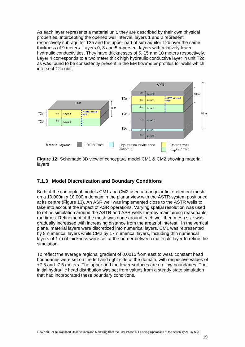
As each layer represents a material unit, they are described by their own physical properties. Intercepting the opened well interval, layers 1 and 2 represent respectively sub-aquifer T2a and the upper part of sub-aquifer T2b over the same thickness of 9 meters. Layers 0, 3 and 5 represent layers with relatively lower hydraulic conductivities. They have thicknesses of 5, 15 and 10 meters respectively. Layer 4 corresponds to a two meter thick high hydraulic conductive layer in unit T2c as was found to be consistently present in the EM flowmeter profiles for wells which intersect T2c unit.
Figure 12: Schematic 3D view of conceptual model CM1 & CM2 showing material layers 7.1.3 Model Discretization and Boundary Conditions Both of the conceptual models CM1 and CM2 used a triangular finite-element mesh on a 10,000m x 10,000m domain in the planar view with the ASTR system positioned at its centre (Figure 13). An ASR well was implemented close to the ASTR wells to take into account the impact of ASR operations. Varying spatial resolution was used to refine simulation around the ASTR and ASR wells thereby maintaining reasonable run times. Refinement of the mesh was done around each well then mesh size was gradually increased with increasing distance from the areas of interest. In the vertical plane, material layers were discretized into numerical layers. CM1 was represented by 8 numerical layers while CM2 by 17 numerical layers, including thin numerical layers of 1 m of thickness were set at the border between materials layer to refine the simulation. To reflect the average regional gradient of 0.0015 from east to west, constant head boundaries were set on the left and right side of the domain, with respective values of +7.5 and -7.5 meters. The upper and the lower surfaces are no flow boundaries. The initial hydraulic head distribution was set from values from a steady state simulation that had incorporated these boundary conditions.

Flow and Solute Transport Observations and Modelling from the First Phase of Flushing Operations at the Salisbury ASTR Site
20
Figure 13: Schematic 3D view of CM2 showing boundary conditions, vertical numerical layers and a plan view of mesh design with expanded view of near-ASTR wells zone.
As seen in Figure 12, the ASTR wells were open over layers 1 and 2 which extend over an 18 m depth, while the Parafield ASR wells (represented in the model as a single well) have an open hole over the entire depth. Time-varying specified flux boundaries were used at the ASTR and ASR wells to create the divergent or convergent flow conditions at the different stages of the trial. To reflect the vertical heterogeneity of the aquifer, flow rates were allocated to each model layer to define the proportion of water which enters the aquifer at the different depths. Assuming that higher transmissivity layers had a higher proportion of flow, rates were defined as: Qi/Q=Ti/T where Q is the total recharge or discharge rate in the well, T the aquifer transmissivity, and Qi and Ti the recharge/discharge rate and the transmissivity relative to the model layer i. As FEFLOW assigns flux boundary conditions at the interface between the two model layers, values set were the mean of the flux of the two adjacent layers. To represent variation in solute concentration due to injection of fresh water, concentration boundaries were set using time-varying specified concentration flux boundaries assigned at the different ASTR injection wells, completed by a flow constraint condition to ensure that no condition was assigned when no flow occurred. A concentration boundary was not set at ASR well as field data suggested that the injectant plume was unlikely to reach the ASTR trial area.
Flow and Solute Transport Observations and Modelling from the First Phase of Flushing Operations at the Salisbury ASTR Site
21
Due to the different phases in the trial, all the simulations were transient both for flow and solute transport, and were usually run over a period of 3 years to limit the computational time. Density effects were not taken into account in the modelling as the salinity contrast between the two end-members waters was insufficient to warrant inclusion (Ward et al., 2008). Temperature changes were ignored as well. 7.1.4 Numerical Methods of Analysis Two numerical methods, based on the solute transport equation, were used to analyse the numerical data. Simulations were set by mixing fraction based on salinity conditions to predict the quality of the recovered water and by decaying tracer concentration to predict residence time of the injected water in the subsurface. Mixing Fraction
Simulations of conservative solute transport were used to predict the mixing and movement of the injected water within the aquifer and therefore the recovered water salinity. Mixing fractions were calculated (defined previously in section 5.1.3) and implemented in FEFLOW using a ‘relative’ solute concentration ranging from 0 to 1 mg/L, set at the value 0 for the ambient groundwater and the value 1 for the injected water. In the following, the mixing fraction was calculated using Cinj = 150 mg/L and Camb = 2000 mg/L based on measured TDS data from the ASTR site (section 6.2.1). Travel Time
Travel time of the fresh water in the aquifer before recovery is required to assess whether sufficient time has elapsed to enable natural attenuation of contaminants within the aquifer. Due to the difficulties resulting from the aquifer heterogeneity which leads to unstable kinematic age computation from a particle tracking method, the effective travel time was calculated using a direct simulation of groundwater age (Goode 1996, Varni and Carrera 1998). Nevertheless, for an easier computational process in transient flow, the method was adapted by assuming a tracer present at some defined concentration in the injected water but absent in the ambient groundwater, and subject to simple exponential decay, as described by the following equation:
( ) efft
o
C t eC
λ−= Equation 5
Where teff is the effective residence time of the water in the aquifer, uncorrected for mixing with the ambient groundwater (d), λ is the decay rate constant (1/d), C(t) is the tracer concentration at some time t (mg/L) and C0 is the tracer concentration in injectant (mg/L). The direct simulation of groundwater age takes into account the effects of dispersion and mixing within the aquifer which tends to exaggerate the minimum residence time of the recovered water by decreasing the tracer concentration used in Equation 5.

Flow and Solute Transport Observations and Modelling from the First Phase of Flushing Operations at the Salisbury ASTR Site
22
Although dilution with ambient groundwater is a physical process that would lower microbial and organic contaminant concentrations, a correction using mixing fraction could be applied to the effective residence time (i.e. ‘uncorrected’ travel time, truncorr) to determine the real age of the injectant to ensure the actual residence time (i.e. ‘corrected’ travel time, trcorr) was reported as described in the Equation below:
( ) ( ) ( )corr uncorrtr t tr t f t= ∗ Equation 6
Nevertheless, as per the approach of Pavelic et al., (2004), no such correction was applied as the magnitude of the change is generally small (<10%).
7.1.5 Calibration Strategy Input parameters are a combination of both physical parameters which represent the hydrogeological system and operational parameters which can be changed by an operator. The aim of the modelling task was to build a predictive tool which can be used to predict the viability of various operational scenarios. Therefore, calibration and adjustment processes were focused on physical parameters, especially on vertical variation induced by heterogeneity in the aquifer. Operational parameters including flow rates, injected and recovered volumes, water quality and storage time were varied from one simulation to another within the range of realistic values assigned from field data. Most physical parameters were considered sufficiently well-known to be directly set from field data (e.g. regional groundwater flow, local gradient from adjacent Parafield ASR operations), or else from the aquifer characterization work (e.g. storage coefficient, aquifer transmissivity), or based on previous studies in the T2 and other literature (e.g. dispersivity, molecular diffusion). Porosity, anisotropy and vertical distribution of hydraulic conductivities were calibrated using a trial-and-error approach during a transient simulation constrained by data on solute breakthrough at observation wells. Parameters used in the calibration process are presented inTable 5. Table 5: Conceptual Model 1 and 2 parameters and values used during the calibration process
Fixed parameters Units Values References Aquifer transmissivity over layers 1 & 2 over entire aquifer
[m2/d] 50 200
AGT (2007) Gerges (2005)
Aquifer thickness [m]] 50 AGT (2007) Storage coefficient [m-1] 2.6x10⁻⁴ AGT (2007) Relative injected concentration [] 1 Relative ambient concentration [] 0 Regional hydraulic gradient [ ] 0.0015 Zulfic (2002) Vertical hydraulic gradient [ ] 0 AGT (2007) Transverse/longitudinal dispersivity ratio [ ] 0.1 Molecular diffusion [m2/s] 1x10⁻⁹ Longitudinal dispersivity [m] 2 Gelhar and Collins
(1971) Adjusted Parameters Units Values Anisotropy Kv/Kh [ ] 0.1, 1 Porosity [ ] 0.25,0.45,0.7 Heterogeneity ratio (x* = Khigher / Klower)
[ ] 1.5, 4, 9

Flow and Solute Transport Observations and Modelling from the First Phase of Flushing Operations at the Salisbury ASTR Site
23
Porosity determines the storage volume in the aquifer and hence influences the ASTR viability by impacting on the effective travel time and the dimension of the injected water plume for a given operational scale. Values used during the calibration process ranged from 0.25 to 0.7. One value of porosity was set for the whole model domain for each simulation. The ASTR viability is also strongly determined by the dispersivity which controls the extent of the mixing zone. In this study, the longitudinal dispersivity was set at 2 m based on previous ASR modelling in the targeted T2 aquifer at the same spatial scale (Pavelic et al, 2002) and the literature (Gelhar and Collins, 1971). Anisotropy influences the vertical mixing and, in this case, determines the flux to and from the T2c sub-aquifer. Values of 0.1 and 1 were used in simulations; 0.1 was expected to lead to a low vertical leakage while a value of 1 was expected to lead to a high vertical leakage and a stronger influence from T2c. To represent aquifer heterogeneity, each material layer was assigned a different hydraulic conductivity value derived from pumping test and EM flowmeter analysis. For both CM1 and CM2, layers 1 and 2, which intersect the open intervals of the ASTR wells, were defined using a heterogeneity ratio x*. x* represents the ratio of the conductivity of the two layers taking account of the ‘higher conductive layer’ and the ‘lower conductive layer’ as described in the aquifer characterization model (Figure 3). Simulations were undertaken using x* = 1.5, 4 and 9, and applied to the average pumping-test-derived value of K = 2.8 m/d interpreted over the aquifer intersected by the ASTR wells. An additional parameterization of CM2, herein referred as CM3, used as well the heterogeneity ratio, but assigned the lower conductive layer in layer 1, and the higher conductive layer in layer 2. This design was expected to yield to a higher contribution from the bottom layers, and especially from the high conductivity layer in T2c. Switching layers 1 and 2, such that the high permeability directly overlies the lower model domain, should maximise the spatial coverage of freshwater/brackish water interface at the base of the open interval, even though it was recognized that the field observations had suggested the opposite was more probable. EM flowmeter analysis and pumping tests were also used to assign hydraulic property in remaining layers in CM2 and CM3. Layer 5 which represents the preferential flow path in aquifer T2c was assigned a value of 65 m/d, scaled from EM flowmeter results. To follow the pumping-test-derived values of 4 m/d interpreted over the T2 aquifer, hydraulic conductivity of lower conductive layers 0, 3 and 5 was set at 0.667 m/d. 7.1.6 Evaluation of Model Performance Eleven simulations were carried out during the calibration process to evaluate the performance of the models CM1, CM2 and CM3 with variation in factors including porosity (ranging from 0.25 to 0.7, vertical leakage (anisotropy varied from 0.1 to 1) and heterogeneity distribution in layer 1 and 2 (Table 6). Input data for each simulation is provided in Appendix 2. The performance of the models was compared with respect to the observed breakthrough derived from 29 EC profiles collected at the injection wells IW1, IW2, IW3 and IW4 during the flushing operations of the Parafield ASTR trial between 2006 and 2007 which implied water injection through recovery wells RW1 and RW2. The goodness of fit measure used was the root-mean-square error (RMSE) and Mean Error (ME) of the mixing fraction (Zheng and Bennett, 1995). While RMSE provides information about the absolute difference between simulated results and field data, ME provides additional information as to whether too much or not enough mixing had occurred (eg. a negative ME means that

Flow and Solute Transport Observations and Modelling from the First Phase of Flushing Operations at the Salisbury ASTR Site
24
the simulated salinity is below the observed salinity concentration and therefore not enough mixing occurred). Further simulations were carried out to assess the hydraulic head of the simulations compared to the observed drawdown at the ASTR wells during pumping test at IW1, IW2 and IW4 (Appendix 3).
7.2 Numerical Results and Discussion
7.2.1 Evaluation of Model Performance Changes in RMSE and ME of mixing fraction for the successive simulations are presented in Table 6. RMSE values ranged from 0.51 (sim1) to 0.08 (sim11). Results showed consistently better performances for CM2 and CM3 than for CM1, with respectively average RMSE of 0.31 for CM1 and 0.19 for CM2-CM3. Negative ME for all simulations using CM1 showed that not enough mixing occurred in the two-layer system. These results suggested that some degree of vertical leakage into the adjacent strata and most notably into T2c must be considered. Two alternative set of parameterization, i.e. CM2 (sim7) and CM3 (sim11), herein referred to as model A and model B were found to fit the field data equally well (Figure 14). The best-fit RMSE was 0.09 for model A and 0.08 for model B. The two models mainly differ in terms of the degree of vertical leakage of recharge water to or from the T2c which is significantly higher in model B, and in term of the storage volume, which is bigger in model A than in model B. The vertical leakage was exacerbated in model B by using an anisotropy value of 1 instead of 0.1 as defined in model A, and by switching the higher and lower conductive layers 1 and 2. The storage volume in layers 1 and 2 was greater in model A than model B using porosity values of 0.7 in model A and 0.25 in model B. Table 6: Summary of adjusted parameters and changes in RMSE of mixing fraction during the calibration process constrained by EC data.
Adjusted parameters Name Model used
Porosity ASR* Kv/KhRMSE f ME f
sim1 0.25 Yes 0.1 0.51 -0.5
sim2 0.45 Yes 0.1 0.3 -0.29
sim3 0.7 Yes 0.1 0.13 -0.08
sim4
CM1
0.7 No 0.1 0.31 -0.28
sim5 0.25 Yes 0.1 0.45 -0.44
sim6 0.45 Yes 0.1 0.18 -0.17
sim7 (Model A) 0.7 Yes 0.1 0.09 0.05
sim8
CM2
0.7 No 0.1 0.19 -0.18
sim9 0.45 Yes 0.1 0.11 0.08
sim10 0.45 Yes 1 0.24 0.21
sim11 (Model B)
CM3
0.25 Yes 1 0.08 0. 05
* ASR refers to the nearby Parafield ASR operations, and was either taken into account in the simulation or neglected as shown

Flow and Solute Transport Observations and Modelling from the First Phase of Flushing Operations at the Salisbury ASTR Site 25
-0.1
0
0.1
0.2
0.3
0.4
0.5
250 300 350 400 450 500 550 600 650 700
Time [d]
Mix
img
fract
ion
Model AModel BField data
IW1
-0.1
0
0.1
0.2
0.3
0.4
0.5
250 300 350 400 450 500 550 600 650 700
Time [d]
Mix
img
fract
ion
Model AModel BField data
IW2
-0.1
0
0.1
0.2
0.3
0.4
0.5
250 300 350 400 450 500 550 600 650 700
Time [d]
Mix
img
fract
ion
Model AField dataModel B
IW3
-0.1
0
0.1
0.2
0.3
0.4
0.5
250 300 350 400 450 500 550 600 650 700
Time [d]
Mix
img
fract
ion
Model AField dataModel B
IW4
Figure 14: Comparison of observed and predicted f versus time at observation wells IW1, IW2, IW3 and IW4 for models A and B, over 684 days of flushing operations at the ASTR site (Time from first injection into RW1 and RW2)

Flow and Solute Transport Observations and Modelling from the First Phase of Flushing Operations at the Salisbury ASTR Site
26
Comparison of the expansion of the fresh injected plume simulated on model A and on model B after 684 days of flushing through RW1 and RW2 clearly showed two very different hydrodynamic behaviours (Figure 15). With high effective porosity and a low vertical leakage, model A simulated a smaller injectant plume, mainly constrained in layers 1 and 2, with a clear preferential flow path in layer 1, the ‘higher conductive layer’ over the open well interval. Model B presented a bigger injectant plume spread in the entire T2 aquifer as expected from a lower effective porosity and a greater leakage. Layer 2, the ‘higher conductive layer’ in the open well interval, and layer 4, the higher conductive layer in T2c can be easily distinguished in the model B plume. Finally, both of the previously described models gave equally good matches with the solute field data at observation wells during the flushing phase while presenting very different hydrodynamic behaviours. At present insufficient field data are available to asses the expansion of the injectant plume within the aquifer, especially in the lower part of the aquifer, allowing the validation of one of these models. Calibration of any groundwater model must contend with the well-known non-uniqueness problem (Chavent, 1974; Yeh, 1986; Freyberg, 1988). Different conceptual models and different sets of parameterization can fit equally well the field data. Solutions to solve the non-uniqueness problem are to collect adequate data fitting the purpose of the study, and limit the likely range of model input (Zheng and Bennett, 1995). To predict mixing and movement of the injected water within the aquifer, models were constrained by transient solute transport which fit the purpose of the study. The range of model input was constrained by field data or literature. One can argue that porosity set at 0.7 for model A is out of the likely range. However, this value is needed to fit the field data if it is assumed that little leakage to and from T2c occurs in this model (Table 6). Simulated mixing processes for this system can be increased by increasing porosity or aquifer dispersivity. When the number of field data is finite and located at limited locations in the spatial domain, and models involve a heterogeneous aquifer, optimal parameterization remains a challenge. Moreover, it has been shown that the ability of a groundwater model to match field data does not necessarily guarantee good prediction under modified conditions (Freyberg, 1988). Therefore, the use of two alternative models offers a good way of judging the reliability of the model predictions, by offering two different approximations of the behaviour of the aquifer system which, thus far, has insufficient data to allow for model validation.

Flow and Solute Transport Observations and Modelling from the First Phase of Flushing Operations at the Salisbury ASTR Site
27
Figure 15: Comparison of mixing fraction distribution simulated on model A and model B for the calibration scenario after 684 days. The horizontal scale is about 250 meters while the vertical scale is 50 meters, encompassing the material layers 0 to 5.
7.2.2 Preliminary Sensitivity Analysis
Sensitivity Analysis on Mixing Fraction
Many numerical studies on ASR/ASTR in similar hydrogeological settings have described the influence of important parameters, such as dispersivity or porosity, on the simulated mixing processes occurring within the aquifer which affects the solute transport (Pavelic et al., 2002, 2004; Lowry et al., 2006). The robustness of the two alternative models A and B models in consistently representing the behaviour of the breakthroughs under different induced stresses allowed a limited sensitivity analysis focused on key parameters. This sensitivity analysis compliments those conducted in previous ASTR studies.
Impacts of Nearby ASR Operations on Mixing Fraction at ASTR Site
RMSE obtained during the calibration process revealed that nearby Parafield ASR operations has a significant effect on salinity values at the observation wells (e.g. difference in RMSE between sim7 and sim8 presented in Table 6). To assess this impact on solute transport in the trial area, three simulations of the flushing phase were run, on both models A and B. The first simulation took into account ASR operations based on data from the field, with a succession of injection and recovery

Flow and Solute Transport Observations and Modelling from the First Phase of Flushing Operations at the Salisbury ASTR Site
28
periods. The second simulation used the same schedule as the previous one but this time injection and recovery periods were inverted. The last simulation did not take ASR operations into account. Comparison of simulated breakthroughs of injectant derived from the three scenarios showed the same general pattern at all the observation wells IW1, IW2, IW3 and IW4 for both of the models. Clear differences in salinity between the three simulations can be observed when no injection occurred at the ASTR (e.g. on Figure 16). For all wells in all cases simulated, the maximum difference in f, occurring between simulations with ASR and inversed ASR when no injection occurred at the ASTR site, is lower than 0.1. Conversely, when injection occurred at the ASTR site, no differences can be distinguished between the different profiles. As no reliable predictions can be done about the likely future operational schedule at the ASR site, and considering that impacts from the ASR site tend to disappear whilst ASTR site is operating, ASR operations will not be taken into account in predictive solute transport simulations of ASTR operations (reported in 7.2.3).
Figure 16: Time versus simulated breakthroughs at IW1 [model A] over 684 days of the flushing period, showing the comparison of three simulations: one taking account of ASR operations, one taking account of inversed ASR operations and one not taking account of ASR operations.
Sensitivity Analysis on Residence Time
Two different methods of analysis were applied to analyse the model results to determine the mixing fraction and residence time. Nevertheless, as both of the methods are based on the solute transport equation, residence time is likely to be affected by the effective porosity and other parameters that affect mixing processes within the aquifer, especially the hydraulic conductivities, anisotropy and dispersivity.

Flow and Solute Transport Observations and Modelling from the First Phase of Flushing Operations at the Salisbury ASTR Site
29
Impacts of Effective Porosity on Residence Time Analysis on the effects of variation in effective porosity on the residence time of the recovered water for CM2 during a simulation of a recovery period after 100 days of injection showed that the residence time decreases as the porosity decreases (Figure 17). Moreover, the minimum time decreases and occurs earlier as the porosity decreases. Simulation with a porosity of 0.7 predicted a minimum residence time 76 days greater and occurring 31 days earlier than for a porosity of 0.45, and 150 days greater and 53 days earlier than for a porosity of 0.25. The two set of parameterization of CM2, model A and model B, presented the same behaviour and the same range of values under variations of porosity.
0
100
200
300
400
500
600
0 20 40 60 80 100 120 140 160 180
Time since first day of pumping [d]
Res
iden
ce ti
me
[d]
n=0.45n=0.25n=0.7
Figure 17: Time since the first day of pumping versus the residence time of the recovered water within the ground (100 days of injection through RW - recovery through IW - no storage period - flow rate at 5L/s - model A). 7.2.3 Predictions of Strategies for Progressing Trial Predictive simulations were carried out to evaluate the mixing between the injected and the ambient groundwater to predict recovered water salinity, and to predict the residence time of the recovered water within the ground. Two potable quality requirements were used to constrain the predictive results of salinity. The first requirement used was a TDS concentration below 500 mg/L (f=0.81) which corresponds to the definition of drinking water in the Australian Drinking Water Guideline. The second requirement used was a salinity below 300mg/L TDS (f=0.92) which is the limit fixed by the City of Salisbury (the ASTR site operators) to fit the intended purpose of the recovered water supplies. Predictive Scenarios - Flushing Stage Firstly, to answer technical questions such as “how much water should be injected into the ground during the flushing phase to ensure the ASTR system meets

Flow and Solute Transport Observations and Modelling from the First Phase of Flushing Operations at the Salisbury ASTR Site
30
performance criteria during the operational phase”, three predictive scenarios have been carried out on both model A and model B. Called ‘scenario 1’, ‘scenario 2’ and ‘scenario 3’, these scenarios simulated three years of the trial, with a ‘flushing phase’, an ‘injection phase’ and a ‘recovery phase’. The same ‘flushing phase’ was used in both scenarios with 338ML flushed into the aquifer from 2006 to 2008 at RW1 and RW2 based on the field data and the same ‘recovery phase’ with 200ML water recovered from RW1 and RW2. They differed on simulating the ‘injection phase’ into the four injection wells with 600ML injected for ‘scenario 1’, 400ML injected for ‘scenario 2’ and 200ML for ‘scenario 3’. Each scenario used an average injection and recovery rate of 5L/s per well; therefore daily fluctuations were not reflected in the simulations.
Prediction of Recovered Water Salinity - Flushing Stage Average salinity concentrations at recovery wells RW1 and RW2 simulated in scenarios 1, 2 and 3 for models A and B are presented on Figure 18. All cases predicted salinity concentrations below 390 mg/L TDS for the first recovery period, and scenario 1 and 2 (respectively 600 and 400 ML flushed during the conditioning phase) predicted concentration below 300 mg/L. That is, a 200 ML injection volume is sufficient to provide water of 500 mg/L but 400 ML or more is needed to achieve 300 mg/L. These results, with respect to the threshold salinities, are the same for both models, although in each scenario model B predicts lower salinity than model A.
150
500
300
0.8
0.9
1
820 920 1020 1120 1220 1320
Time [d]
Mix
ing
fract
ion
Model A scenario 1 Model A scenario 2 Model A scenario 3Model B scenario1 Model B scenario 2 Model B scenario 3
TDS
[mg/
L]
Figure 18: Time versus average simulated salinity concentration at recovery wells RW1 and RW2 during the conditioning phase of the ASTR trial, for scenarios 1, 2 and 3, for models A and B.
Predictive Scenarios - Operating Stage To evaluate the impact of each different flushing case on recovered water quality in the subsequent operational stage, three simulations referred to as ‘cycle a’, ‘cycle b’ and ‘cycle c’ representing injection/recovery cycles during normal, dry and wet years, respectively were created. These cycles, run over 6 years, were initialised from head and solute distributions derived from simulation of the ‘conditioning scenarios’. They

Flow and Solute Transport Observations and Modelling from the First Phase of Flushing Operations at the Salisbury ASTR Site
31
all represent a succession of injection and recovery phases designed to correspond to seasonal variations of water supplies with the injection period during winter months and recovery during summer months. In each cycle it was specified that 80% of the injected volume is recovered in the following recovery, to ensure a good buffer against the brackish water in the storage zone over the following years. ‘Cycle a’ representing a normal year of use simulated 100 days of injection during winter with 172.8 ML/yr stored in the aquifer, ‘cycle b’ representing wet years involved 300 ML/yr of water stored in the ground over 174 days, and ‘cycle c’ representing dry years simulated 104 ML/yr stored during 60 days of injection. Assumptions of annual volume of injected water were based on field average injection rate of 5 L/s and the number of days of availability of stormwater.
Prediction of Recovered Water Salinity - Operating Stage To assess the effects of the initial flushing volume on the system efficiency over the long term, comparison of the history of the average concentration at the two recovery wells for each of the three flushing scenarios followed by a ‘normal’ injection/recovery cycle (cycle a) over 6 years for both model A and B are presented on Figure 19. Predicted concentrations differed between models A and B with a better quality predicted for model B. Both models predicted for all cases recovered water salinity below 500 mg/L TDS. Model B, for scenario 1 and 2, predicted concentrations below 300 mg/L TDS. Despite the differences in concentration between models, the general patterns of the profiles simulated by model A and model B appeared to be quite similar. For each case, the salinity concentration increases during the first years before stabilizing at an equilibrium value. The magnitude and the persistence of the dip varied for each scenario, which is a function of the amount of water used for flushing. The smallest amount of water injected during the conditioning phase (200 ML - scenario 3) gave the highest and most persistent increase in TDS. Both models show that greater flushing volumes reduce the salinity of recovered water but with diminishing efficiency as the flushing volume increased from 400 ML to 600 ML.

Flow and Solute Transport Observations and Modelling from the First Phase of Flushing Operations at the Salisbury ASTR Site
32
500
150
300
0.8
0.9
1
Mix
ing
fract
ion
Model A - scenario 1aa
Model A - scenario 2aa
Model A - scenario 3aa
TDS [m
g/L]
500
150
300
0.8
0.9
1
Mix
ing
fract
ion
Model B - scenario 1aaModel B - scenario 2aa
Model B - scenario 3aa
TDS [m
g/L]
Figure 19: Effect of volume of water injected during the first injection period through IW1, IW2, IW3 and IW4 on recovered water salinity at RW1 and RW2, simulated on model A and model B. Comparison of salinity concentration at the recovery wells for cycles a, b and c after the flushing scenarios 1, 2 and 3 are presented in Table 7. It appears that average values from the different cycles after a given flushing scenario, and for one given model, are almost identical. Therefore, simulated water quality of the recovered water during the first six years of the trial depends more on the flushing scenario and on the
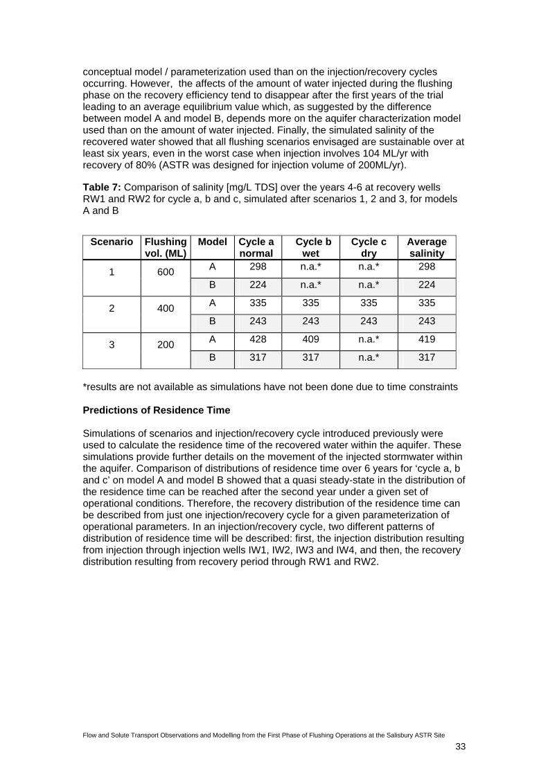
Flow and Solute Transport Observations and Modelling from the First Phase of Flushing Operations at the Salisbury ASTR Site
33
conceptual model / parameterization used than on the injection/recovery cycles occurring. However, the affects of the amount of water injected during the flushing phase on the recovery efficiency tend to disappear after the first years of the trial leading to an average equilibrium value which, as suggested by the difference between model A and model B, depends more on the aquifer characterization model used than on the amount of water injected. Finally, the simulated salinity of the recovered water showed that all flushing scenarios envisaged are sustainable over at least six years, even in the worst case when injection involves 104 ML/yr with recovery of 80% (ASTR was designed for injection volume of 200ML/yr). Table 7: Comparison of salinity [mg/L TDS] over the years 4-6 at recovery wells RW1 and RW2 for cycle a, b and c, simulated after scenarios 1, 2 and 3, for models A and B
Scenario Flushing vol. (ML)
Model Cycle a normal
Cycle b wet
Cycle c dry
Average salinity
A 298 n.a.* n.a.* 298 1 600 B 224 n.a.* n.a.* 224
A 335 335 335 335 2 400 B 243 243 243 243
A 428 409 n.a.* 419 3 200 B 317 317 n.a.* 317
*results are not available as simulations have not been done due to time constraints Predictions of Residence Time Simulations of scenarios and injection/recovery cycle introduced previously were used to calculate the residence time of the recovered water within the aquifer. These simulations provide further details on the movement of the injected stormwater within the aquifer. Comparison of distributions of residence time over 6 years for ‘cycle a, b and c’ on model A and model B showed that a quasi steady-state in the distribution of the residence time can be reached after the second year under a given set of operational conditions. Therefore, the recovery distribution of the residence time can be described from just one injection/recovery cycle for a given parameterization of operational parameters. In an injection/recovery cycle, two different patterns of distribution of residence time will be described: first, the injection distribution resulting from injection through injection wells IW1, IW2, IW3 and IW4, and then, the recovery distribution resulting from recovery period through RW1 and RW2.
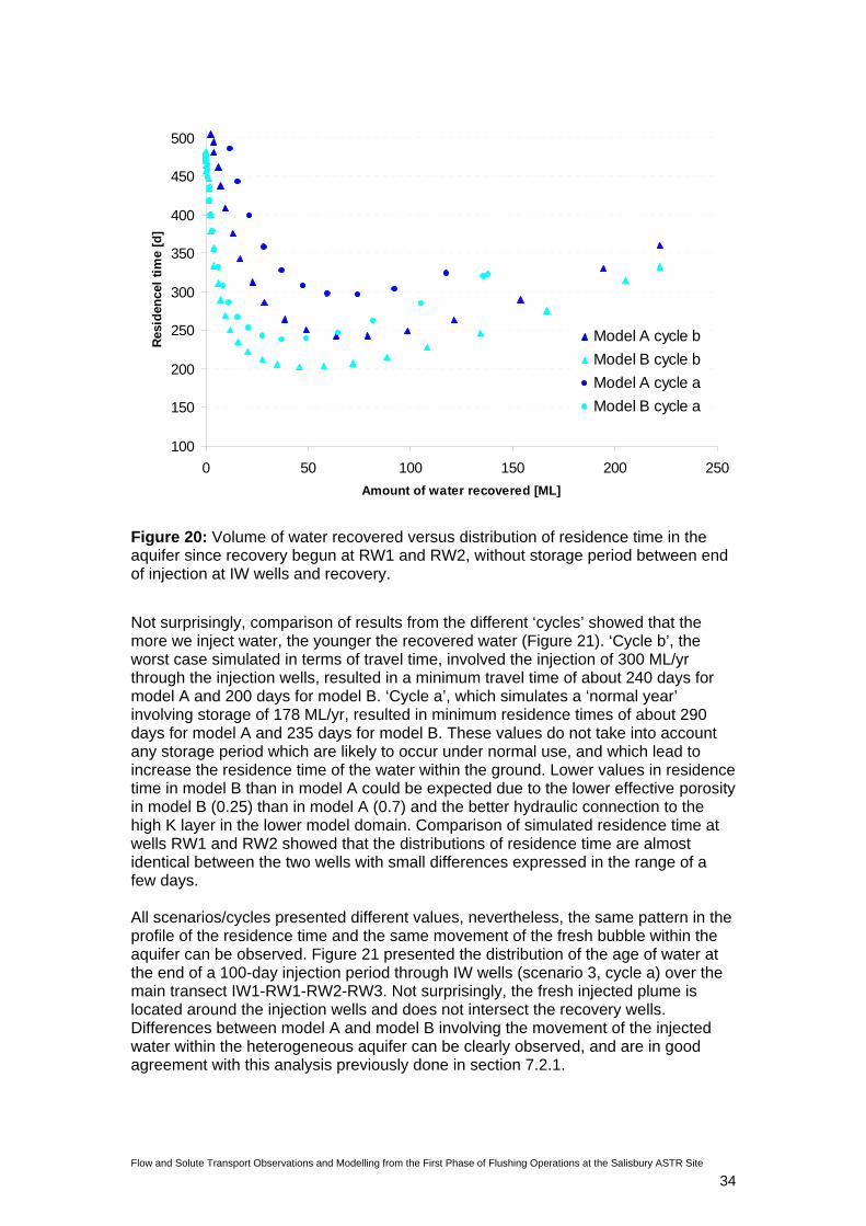
Flow and Solute Transport Observations and Modelling from the First Phase of Flushing Operations at the Salisbury ASTR Site
34
100
150
200
250
300
350
400
450
500
0 50 100 150 200 250Amount of water recovered [ML]
Resi
denc
el ti
me
[d]
Model A cycle bModel B cycle bModel A cycle aModel B cycle a
Figure 20: Volume of water recovered versus distribution of residence time in the aquifer since recovery begun at RW1 and RW2, without storage period between end of injection at IW wells and recovery.
Not surprisingly, comparison of results from the different ‘cycles’ showed that the more we inject water, the younger the recovered water (Figure 21). ‘Cycle b’, the worst case simulated in terms of travel time, involved the injection of 300 ML/yr through the injection wells, resulted in a minimum travel time of about 240 days for model A and 200 days for model B. ‘Cycle a’, which simulates a ‘normal year’ involving storage of 178 ML/yr, resulted in minimum residence times of about 290 days for model A and 235 days for model B. These values do not take into account any storage period which are likely to occur under normal use, and which lead to increase the residence time of the water within the ground. Lower values in residence time in model B than in model A could be expected due to the lower effective porosity in model B (0.25) than in model A (0.7) and the better hydraulic connection to the high K layer in the lower model domain. Comparison of simulated residence time at wells RW1 and RW2 showed that the distributions of residence time are almost identical between the two wells with small differences expressed in the range of a few days. All scenarios/cycles presented different values, nevertheless, the same pattern in the profile of the residence time and the same movement of the fresh bubble within the aquifer can be observed. Figure 21 presented the distribution of the age of water at the end of a 100-day injection period through IW wells (scenario 3, cycle a) over the main transect IW1-RW1-RW2-RW3. Not surprisingly, the fresh injected plume is located around the injection wells and does not intersect the recovery wells. Differences between model A and model B involving the movement of the injected water within the heterogeneous aquifer can be clearly observed, and are in good agreement with this analysis previously done in section 7.2.1.

Flow and Solute Transport Observations and Modelling from the First Phase of Flushing Operations at the Salisbury ASTR Site
35
Figure 21: Comparison of simulated distribution of the age of water at the end of an injection period through IW wells (scenario 3a) over the main transect IW1-RW1-RW2-RW3. The horizontal scale is about 250 meters while the vertical scale is 50 meters, encompassing the material layers 0 to 5. When recovery occurs, the fresh injected bubble is drawn towards the recovery wells RW1 and RW2. Results of injection/recovery cycle simulations clearly showed the displacement of the fresh plume towards the recovery wells (Figure 20). In all cases, a minimum residence time corresponding to the breakthrough of the fresh plume at the recovery wells appeared after about 30-60 ML is recovered (35-70 days of pumping at the average rate of 5 L/s) with a minimum residence time of 235 days under normal operational conditions (178 ML/yr). After reaching this minimum value, residence times increase following a linear evolution in function of time. The oldest residence times appeared at the beginning of the pumping phase with values around 450 and 500 days.

Flow and Solute Transport Observations and Modelling from the First Phase of Flushing Operations at the Salisbury ASTR Site
36
8 CONCLUSION Field Trial Actual flushing operations at the ASTR trial site have involved the injection of about 338ML of stormwater through wells RW1 and RW2 by June 2008. First EC observations at observation wells IW1, IW2, IW3 and IW4 showed clear breakthrough of the injectant across the study zone, and by June 2008 73% breakthrough had occurred at these wells. Solute observations of the breakthrough of injectant were conducted by downhole profiling in the four IW wells which are completed with long open intervals (18 m). Intra-well flow is suspected to have occurred in these wells; however there was insufficient data to enable a detailed investigation of intra-well flow processes.
Flow and Solute Transport Modelling Flow and solute transport processes at the ASTR trial site were reliably simulated using a 3D model that used a layer-cake structure to describe the heterogeneity within the aquifer. The best calibration results were achieved through the use the 6-material-layered model (CM2) which encompasses T2a,b and c sub-aquifers as compared to the 2-material-layered model (CM1) which only describes T2a,b. CM2 is justified to take account of the vertical leakage to and from T2c. Two alternative models derived from CM2, model A and model B, appear to be consistent for the preliminary predictive scenarios with very similar breakthrough curves. Nevertheless, models A and B have significantly different hydrodynamic profiles, and, thus far, there is too few field data to determine which of the two models is the more appropriate. Model B would appear to be more realistic than model A, which has a porosity of 0.7. The methods of analysis using conservative solute transport to predict the mixing between the two-end members and the residence time within the aquifer proved to be effective in an ASTR context. Predictions of Operations for Progressing Trial Results of nine-year injection/recovery cycles at the ASTR trial showed that the efficiency of the system will depend more on the amount of water injected in the aquifer during the conditioning phase than on the volume of water available for injection each year. Predictions of the quality of the recovered water showed that, thus far, enough water (338ML) has been injected through recovery wells to ensure potable quality largely below the 500 mg/L TDS drinking water guideline over the long term, even under drought conditions. Scenarios involving additional flushing volumes of 400 and 600 ML in the IW wells predicted that the salinity of the recovered water would remain below 300 mg/L TDS for the first recovery period. Over the longer term, predicted salinity depends more on the aquifer characterization model used than on the operational parameters set. Over 6 years, for 400 ML and 600 ML of simulated flushing in the second phase through the IW wells after the first phase of RW flushing, model A predicted salinity below 390 mg/L while model B predicted salinity below 300 mg/L. The minimum residence time simulated under normal conditions appeared to be greater than 200 days, which is considered to provide sufficient residence time for natural attenuation of microbial contaminants.

Flow and Solute Transport Observations and Modelling from the First Phase of Flushing Operations at the Salisbury ASTR Site
37
9 RECOMMENDATIONS Strategies for Progressing Trial A first complete injection/recovery cycle of 200 ML/yr following the conclusion of the flushing phase would produce potable water quality with a salinity below 300 mg/L TDS for the first year and 500 mg/L for the following years. Nevertheless, it is recommended that 400 ML should be injected through the IW wells during the next phase of flushing to ensure more reliable and long-term quality of the recovered water to fulfil the requirements of achieving a salinity below 300 mg/L TDS. Field Monitoring Further field data from the drilling of three new piezometers at the trial site with short open intervals (3-4 m) will be required to: (a) allow validation of previous observations; (b) give more reliable monitoring data for future modelling; and (c) to assist in differentiating between the candidate models. At the time of writing the new piezometers had been constructed along the main transect between IW1 and IW3 (their locations are shown in Figure 1) but there was insufficient opportunity to collect or analyse water level or water quality data. In future, downhole EC and temperature loggers should be installed within the open interval of each of the piezometers and in the delivery line to the IW wells to track short and medium term EC/temperature fluctuations in source water within the aquifer for the determination of travel times. Additional independent measures for travel time may warrant evaluation, including the use of natural or artificial tracers. Further Modelling For future groundwater modelling to develop a revised model which will help to reliably interpret the field data and assist in refining the operating schedule during normal ASTR operations beyond the flushing phase, the following actions are recommended:
(1) Refinement and validation of the models, using additional field data from the new piezometers at the trial site as well as from porosity and pore-water salinity measurements on core samples collected during drilling of the deepest piezometer (P2). Such refinements should include enhanced vertical discretization in layer 3 to determine whether numerical dispersion has significantly affected the downward movement of solutes from layers 1 and 2.
(2) Consideration of the sensitivity of the residence time and mixing fraction predictions under different operational conditions, notably the impact of a pumping rate of 10L/s which may be implemented during the field trial and possible recovery during injection.
(3) Integration of hydraulic head data in the next phase of calibration to refine the model.
(4) Revisiting the original design to inject into T2ac to determine whether the additional data used to refine the model, if available initially, would have resulted in acceptance of that design.
(5) Accounting for anomalies if encountered by incorporating heterogeneity within the horizontal plane, and performing sensitivity analyses on the final calibrated model.
(6) Exploring alternative ASTR designs, including intermittent multi-well systems.
Flow and Solute Transport Observations and Modelling from the First Phase of Flushing Operations at the Salisbury ASTR Site
38
REFERENCES AGT (2007) Final draft Parafield ASTR wells completion report and aquifer test results. AGT Report no 2077/22, Australian Groundwater Technologies PTY LTD, Wayville, South Australia.
Chavent, G., (1974) Identification of Parameters in Distributed Systems, Goodson, R. E. and M. Polis, pp. 31-48, American Society of Mechanical Engineers, New York.
Church, P.E. and Granato, G.E. (1996) Bias in ground water data caused by well-bore flow in long-screen wells. Ground Water 34, no.2, pp. 262-276.
Cooper, H.H. and C.E. Jacob (1946) A generalised graphical method for evaluating formation constants and summarising will field history, Am. Geophys. Union Trans., vol. 27, pp.526-534.
Diersch, H.-J. (2004) FEFLOW: Interactive, graphics-based finite-element simulation system for modelling groundwater flow, contaminant mass and heat transport processes. Getting Started; User’s Manual; Reference Manual, Version 5.1. WASY, Institute for Water Resources Planning and System Research Ltd, Berlin, Germany.
Dillon, P., Page, D., Pavelic, P., Toze, S., Vanderzalm, J., Barry, K., Levett, K., Regel, R., Rinck-Pfeiffer, S., Pitman, C., Purdie, M., Marles, C., Power, N. and Wintgens, T. (2008) City of Salisbury’s progress towards being its own drinking water catchment. In: Singapore International Water Week, Singapore, 23-27 June 2008.
Elci, A., Moltz, F.J. and Waldrop, W.R. (2001) Implications of Observed and Simulated Ambient Flow in Monitoring Wells. Ground Water, vol. 39, no. 6, pp.853-862.
Freyberg, D.L. (1988) An exercise in ground water model calibration and prediction. Ground Water vol. 26, no.3, pp.350-360.
Gelhar, L.W. and Collins, M.A. (1971) General analysis of longitudinal dispersion in nonuniform flow. Water Resources Research vol. 7, no. 6, pp. 1511-1521.
Georgiou, J.P. (2002) Conceptual and Field Modelling of Flow And Transport In a Multi-Layer Aquifer: Effects Of Fully Penetrating Wells. Honours Thesis, Flinders University of South Australia.
Gerges, N., Z. (1999) The geology and hydrogeology of the Adelaide metropolitan area. PhD Thesis, Flinders University of South Australia.
Gerges, N.Z. (2005) Greenfield Railway Station ASTR Project Briefing on Aquifer Tests. NZG Groundwater Consultant, Hallett Cove SA 5158, Australia.
Goode, D.J. (1996) Direct simulation of groundwater age. Water Resources Research, vol. 32, no. 2, pp. 289-296.
Güven, O., Molz, F.J., Melville J.G., El Didy S. and Boman G.K. (1992) Three-dimensional modelling of a two-well tracer test. Ground Water 30, no. 6, pp. 945-957.
Hutchins, S.R. and Acree, S.D. (2000) ground water sampling bias observed in shallow conventional wells. Ground Water Monitoring & Remediation 20, no.1: 86-93.
Lowry, C. S. and Anderson, M.,P. (2006) An Assessment of Aquifer Storage and Recovery Using Ground Water Flow Models. Ground Water, vol. 44, no. 5, pp.661-667.
Molz, F.J.; Morin, R.H.; Hess, A.E.; Melville, J.G.; Güven, O. (1989) The Impeller Meter for Measuring Aquifer Permeability Variations: Evaluation and comparison With Other Tests. Water Resour. Res., vol. 25, no. 7, pp. 1677-1683.

Flow and Solute Transport Observations and Modelling from the First Phase of Flushing Operations at the Salisbury ASTR Site
39
Molz, F.J., Boman G.K., Young, S.C. and Waldrop, W.R. (1994) Borehole flowmeters: Field application and data analysis. Journal of Hydrology 163, no.3-4, pp.347-371
Page, D., Barry, K., Chassagne, A., Pavelic, P., Dillon, P., Purdie, M., Pittman, C., Rinck-Pfeiffer, S. and Regel, R. (2007) Application of the Hazard Analysis and Critical Control Point (HACCP) risk management framework to managed aquifer recharge. Proceedings of the 6th International Symposium on Management of Aquifer Recharge (ISMAR6), Phoenix 28 Oct-2 Nov. 2007, Ed. P. Fox, Acacia Publishing, Phoenix, Arizona, pp.578-589.
Pavelic, P., Dillon, P.J. and Simmons, C. T. (2006) Multiscale Characterization of a Heterogeneous Aquifer Using an ASR Operation. Ground Water vol. 44, no.2, pp. 155-164.
Pavelic, P., Dillon, P.J., Barry, K., Vanderzalm, J., Le Gal La Salle, C., Georgiou J., Simmons, C. T. and Martin, R. (2005) Flow and solute transport: field observations and modelling aspects. In: Martin, R. and Dillon, P (eds) Bolivar Reclaimed Water Aquifer Storage and Recovery Research Project Final Report. Department Water, Land, Biodiversity and Conservation Report No. DWLBC 2005/44.
Pavelic, P., Dillon, P. and Robinson, N. (2004) Groundwater Modelling to Assist Well-Field Design and Operation for the ASTR Trial at Salisbury, South Australia. CSIRO Land and Water Technical Report No. 27/04.
Pavelic, P., Dillon P.J. and Simmons, C.T. (2002) Lumped parameter estimation of initial recovery efficiency during aquifer storage and recovery. In: Dillon, P.J. (ed) Management of Aquifer recharge for Sustainability. Swets and Zeitlinger, Lisse, ISBN 90 5809 527 4.
Reilly, T.E., Frank, O.L. and Bennett, G.D. (1989) Bias in groundwater samples caused by wellbore flow. ASCE, Journal of Hydraulic Engineering 115, pp. 270-276.
Rinck-Pfeiffer S, Pitman C, Dillon, P (2005). Stormwater ASR and ASTR (Aquifer Storage Transfer and Recovery) in practice and under investigation in South Australia. In: Recharge systems for protecting and enhancing groundwater resources. Proceedings of the 5th International Symposium on Management of Aquifer Recharge (ISMAR5), Berlin, Germany, 11-16 June 2005. IHP-VI Series on Groundwater No. 13.
Swierc J, Page D, van Leeuwen J, and Dillon P (2005). Preliminary Hazard Analysis and Critical Control Points Plan (HACCP) - Salisbury Stormwater to Drinking Water Aquifer Storage Transfer and Recovery (ASTR) Project, CSIRO Land and Water Technical Report 20/05.
Varni, M. and Carrera, J. (1998) Simulation of groundwater age distribution. Water Resources Research, vol. 34, no. 12, pp. 3271-3281.
Ward, J.D., C.T. Simmons and P.J. Dillon (2008) Variable-density modelling of multiple-cycle aquifer storage and recovery (ASR): Importance of anisotropy and layered heterogeneity in brackish aquifers. Journal of Hydrology vol. 356, pp. 93-105
Yeh, W.G. (1986) Review of Parameters Identification Procedures in Groundwater Hydrology: The Inverse Problem. Water Resources Research, vol. 22, no. 2, pp. 95-108.
Zheng, C. and Bennett, G. D. (1995) Applied Contaminant Transport Modelling: Theory and Practice Van Nostrand Reinhlod/ International Thomson Publishing Inc.
Zulfic, H. (2002) Northern Adelaide Plains Prescribed Wells Area ground water monitoring report. Department Water, Land, Biodiversity and Conservation Report DWLBC 2002/14.
Flow and Solute Transport Observations and Modelling from the First Phase of Flushing Operations at the Salisbury ASTR Site
40
APPENDIX 1: Overview of 3D Model Simulations of ASTR That Take
Heterogeneity into Account, Carried Out in 2005 In light of the downhole EM flowmeter data collected in 2005 which had identified that the aquifer was more heterogeneous than had been previously anticipated, further FEFLOW simulations were performed by CSIRO between late 2005 and early 2006 to assess whether the ASTR well-field design proposed by Pavelic et al., (2004) consisting of six wells, spaced 75m apart and completely penetrating the T2 aquifer, could still meet the required salinity and travel time criteria. These simulations examined a range of design considerations that included:
• reducing the well-spacing from 75 m to 50 m • installing partially penetrating (T2a,b) wells versus completely penetrating (T2a,b,c)
wells • effects of pre-existing Parafield ASR operations if the ASTR well-field was shifted
closer to that ASR system • reduction in the operational scale from 400 ML/yr to 200 ML/yr associated with
partially penetrating injection/recovery wells • varying the volumes of water used to flush the aquifer in the first year of operation • targeting the overlying T1 aquifer instead of the T2 • completing wells in upper sequence (T2a,b) versus the entire aquifer sequence
(T2a,b,c) An inventory of the key model parameters and model outputs are presented in the table below. Simulations are numbered 27 through to 75. Generally paired sets of simulations were performed; one to enable mixing fractions to be calculated, the other for residence times. It was concluded that due to aquifer heterogeneity, ASTR at 75 m spacing would not meet the performance targets. Reducing the well spacing to 50 m had the potential to provide a viable scheme if the aquifer transmissivity was high enough to enable sufficient stormwater to be stored in the aquifer. Following discussions between project partners when the interim modelling results were presented, it was recommended that the trial should proceed with a six-well array 200ML/yr ASTR scheme with wells open over T2a,b at an inter-well spacing of 50 m if a transmissivity of around 50 m2/day was measured in the upper part of the T2 formation, allowing for at least 10 m of vertical separation with the underlying high K layer known to be present in T2c. The fully-penetrating well GRS1, drilled as an intended production well at the GRS station, was partially backfilled and the transmissivity re-assessed by pump testing to be approximately 50 m2/day (N.Z. Gerges, pers. comm.). Having established that a 50 m spacing was needed and that a transmissivity of 50 m2/day was feasible in T2a,b, the location of the ASTR well-field site was shifted from the vicinity of the Greenfield Railway Station to the Parafield Gardens Oval site. This shift was on the basis that:
• the oval site had not been initially considered due to broader well spacing (75 m vs 50 m) rendering the site unsuitable
• all of the wells could be grouped together on City of Salisbury land rather than dispersed on both council and private property on two sides of a major stormwater drain and railway line
• the modelling had predicted there would be no significant hydraulic interaction between the Parafield ASR and the ASTR well field if situated at the oval site
• security was considered much better at the oval site compared to the railway station site

Flow and Solute Transport Observations and Modelling from the First Phase of Flushing Operations at the Salisbury ASTR Site
41
• the well drilled for the project near the Greenfields railway station (GRS1) could be used as an observation well
The simulation-pair #76 and #77 that was considered to best represent the likely conditions at the ASTR site. This model consisted of a 35 m thick, four-layer aquifer, as per the heterogeneity structure at the Bolivar ASR site (Pavelic et al., 2006), with a thickness of 35 m porosity of 0.25. Essentially this is a model with a thickness intermediate to CM1 and CM2, but more closely aligned to CM1 since it only considers the open interval of the injection and recovery wells. It should be noted that the storage capacity of the aquifer for this model construct (determined from the product of aquifer thickness and porosity), is about 30% lower than either CM1 or CM2. Over the first three years of operation, the minimum mixing fraction in the recovered water of this model is predicted to be 0.89. The predicted recovery efficiency in the third year of operation (using f=0.9 as the lower limit) was predicted to be 74% if 400 ML of water were available for flushing in the first year of operation, or a 90% recovery efficiency if 500ML were available over that same period. The minimum residence time of the recharge water was almost 250 days. The reduction in operational scale from 400 ML/yr to 200 ML/yr was necessary on account of the lower injection rate anticipated for wells that intersect only the upper part of the aquifer. Legend
Spac. = inter-well spacing between injection and recovery wells (m) Trans. = aquifer transmissivity (m2/day) Layers = number of material layers that the aquifer is assumed to be composed of b = thickness of aquifer (m) Qi = injection rate (L/s) Qr = recovery rate (L/s) Vi = volume of water injected (ML) Vr = volume of water recovered (ML) hmax = maximum groundwater level increase above static levels within model domain, always at an injection well (m) fmin = minimum mixing fraction in recovered water, average of the two recovery wells (m) tres = residence time of the injectant in the aquifer (days)

Flow and Solute Transport Observations and Modelling from the First Phase of Flushing Operations at the Salisbury ASTR Site 42
Model outputs: Sim No.
Aquifer Spac (m)
Trans(m2/d)
Lay-ers
b (m) x* Qi/r (L/s)
Vi (ML)
Vr (ML)
Comments
hmax fmin tres (d)
10-27 T2 75 125 1 35 1 25 400 320 Homogeneous 2D base-case simulation from Pavelic et al, (2004)
~43 0.992 ND
30-31 T2 75 125 4 35 4 25 400 320 ~43 0.976 273 32-33 T2 75 125 4 35 9 25 400 320 ~43 0.945 266 28-29 T2 75 125 4 35 24 25 400 320 3D Base-case simulation 43.2 0.920 253
38a T2 75 50 4 35 24 6.25 400 320 39.8 ND ND
38b T2 75 50 4 35 24 12.5 400 320 79.5 ND ND
38c T2 75 50 4 35 24 25 400 320 * hydraulic s/state simulations only 133.2 ND ND
38d T2 75 100 4 35 24 6.25 400 320 ** Sims also done for T=125&300 m2/d; 20.0 ND ND
38e T2 75 100 4 35 24 12.5 400 320 for cyclic operation of wells and for 39.8 ND ND
38f T2 75 100 4 35 24 25 400 320 4-well array 79.5 ND ND
38g T2 75 200 4 35 24 6.25 400 320 10.1 ND ND
38h T2 75 200 4 35 24 12.5 400 320 20.0 ND ND
38i T2 75 200 4 35 24 25 400 320 40.0 ND ND
39-40 T2 75 50 4 35 24 12.5 400 320 assess Qi/r effect on fmin and tres (sims 39/40 cf. 41/42)
~79.5 0.917 248
41-42 T2 75 50 4 35 24 25 400 320 assess Trans. Effect on fmin & tres (sims 28/29 cf sims 41/42)
~43 0.917 253
43 T2 75 125 4 35 24 25 400 320 alpha-L = alpha-T=5m ~43 0.965 ND
44 T2 75 125 4 35 24 25 400 320 alpha-L = alpha-T=5m & Kh=Kv ~43 0.965 ND
48 T2 75 50 4 35 24 12.5 400 320 400ML in first year rather than 1000ML ~79.5 0.899 ND
53-54 T2 75 50 4 35 24 6.25 200 160 ½ - scale (500ML) - f declines expected to continue
26.6 0.871 348
57 T2 75 50 4 35 24 6.25 200 160 As per sim 53 but pumping stops at f=0.9 in year 2
26.6 0.886 348
58 T2 75 125 4 35 24 25 400 320 Replica of 28, but with multi-aquifer BC’s 43.1 0.881 ND
59-61 T2 75 50 4 35 24 6.25 200 197 b Inc. gradients due to Parafield (RE-yr3=0%) 27.6 0.857 353
60 T2 75 50 4 35 24 6.25 200 197 b As per sim 59 but pumping stops at f=0.9 in year 2 (RE-yr3 = 58% = 116ML)
“ 0.874 “

Flow and Solute Transport Observations and Modelling from the First Phase of Flushing Operations at the Salisbury ASTR Site 43
62 T2 75 50 4 35 24 6.25 200 197 b As per sim 60 with gradients due to Parafield removed (RE-yr3 = 53% = 105ML)
27.2 0.873 353+
67-68 T2 75 50 4 35 24 6.25 200 197 b * 50 m SPACING. As per sims 59&61 in all other respects (RE-yr3 = 90% = 179ML)
30.0 0.89 247
76-77 T2 50 50 4 35 24 6.25 200 197 b * 50 m SPACING Inc. Parafield grads–located closer (RE-yr3=74%=147ML)
31.2 0.89 246
69 T2 50 50 4 35 24 6.25 200 197 b * 50 m SPACING. As per #67 but with 400ML of flushing in yr1, not 500ML (RE-yr3 =74% = 148ML)
30.0 0.866 247
72-73 T1+T2
50 50+69 5 60 24 6.25 200 197 b * 50 m SPACING, T1 analogue - low gradients (RE-yr3 =0% )
15.6 0.840 280
74-75 T1+T2
50 50+69 5 60 24 6.25 200 197 b * 50 m SPACING, T1 analogue-typical gradients (RE-yr3 =0% )
~16 0.843 277
63-64 T2 75 125 4 35 24 12.5 400 394 c Inc. gradients due to Parafield (RE-yr3 = 99% = 394ML)
24.6 0.900 254
65 T2 75 125 4 35 24 12.5 400 394 c As per sim 63 with gradients due to Parafield removed (RE-yr3 = 101% = 403ML projected
23.6 0.902 “
66 T2 75 125 4 35 24 12.5 400 394 c As per #63 but with 500ML in yr 1 and not 1000ML (RE-yr3 = 75% = 300ML)
24.6 0.871 254
70-71 T2 50 125 4 35 24 12.5 400 394 c * 50 m SPACING. As per sim 66. RE-yr3=91% =362ML)
26.4 0.888 179
34-35 T2 75 125 3 35 30 25 400 320 ~<43 0.582 78
36-37 T2 75 125 3 35 30 25 400 320 4-well case (rather than 6-well for sims 34/35) ~<43 0.501 105
55-56 T2 75 150 3 15 650 25 400 320 Most realistic simulation of inj/rec in lower formation
41.1 0.682 42*
45 T2 75 200 7 50 24&30 25 400 320 (-) Injection and recovery into upper only 57.2 0.928 ND
46-47 T2 75 200 7 50 24&30 12.5 400 320 13.5 0.836 205
49-50 T2 75 200 7 50 24&30 12.5 400 320 Separation distance reduced from 75m to 50m ~<20 0.873 92
51-52 T2 75 200 3 50 72 25 400 320 Mixing fractions in yrs 4-7 decrease further (min=0.57)
24.5 0.721 129
ND = not determined; 1) hmax = maximim head (above static level) at injection wells; 2) fmin = mixing fraction at end of pumping in year 3 (avg of 2 wells); 3) tres refers to minimum residence time in year 3 (avg of 2 wells); a taken from S/State analysis results; b160ML in yr 2 and 197ML in yr 3; c 320ML in yr 2 and 394ML in yr 3
* parameter values used in all simulations: longitudinal dispersivity = 5m; transverse dispersivity = 0.5m; porosity = 0.25

Flow and Solute Transport Observations and Modelling from the First Phase of Flushing Operations at the Salisbury ASTR Site 44
APPENDIX 2:
Input Data for Modelling Input data for modelling scenarios 1, 2 and 3 Scenario 1 Injection/recovery rate [m3/d]
Time* [d] RW1 RW2 IW1 IW2 IW3 IW4
250-367 -367.5 -300 0 0 0 0
486-820 -423 -359 0 0 0 0
830-1177 0 0 -432 -432 -432 -432
1180-1580 600 600 0 0 0 0
Scenario 2 Injection/recovery rate [m3/d]
Time* [d] RW1 RW2 IW1 IW2 IW3 IW4
250-367 -367.5 -300
486-820 -423 -359
830-1030 -500 -500 -500 -500
1040-1240 500 500
Scenario 3 Injection/recovery rate [m3/d]
Time* [d] RW1 RW2 IW1 IW2 IW3 IW4
250-367 -367.5 -300 0 0 0 0
486-820 -423 -359 0 0 0 0
830-946 0 0 -432 -432 -432 -432
956-1156 500 500 0 0 0 0
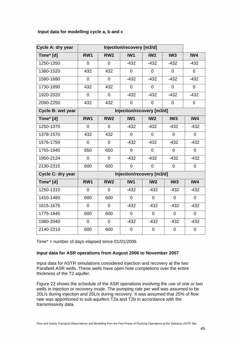
Flow and Solute Transport Observations and Modelling from the First Phase of Flushing Operations at the Salisbury ASTR Site 45
Input data for modelling cycle a, b and c
Cycle A: dry year Injection/recovery [m3/d]
Time* [d] RW1 RW2 IW1 IW2 IW3 IW4
1250-1350 0 0 -432 -432 -432 -432
1360-1520 432 432 0 0 0 0
1580-1680 0 0 -432 -432 -432 -432
1730-1890 432 432 0 0 0 0
1920-2020 0 0 -432 -432 -432 -432
2090-2250 432 432 0 0 0 0
Cycle B: wet year Injection/recovery [m3/d]
Time* [d] RW1 RW2 IW1 IW2 IW3 IW4
1250-1370 0 0 -432 -432 -432 -432
1378-1570 432 432 0 0 0 0
1576-1750 0 0 -432 -432 -432 -432
1755-1940 650 650 0 0 0 0
1950-2124 0 0 -432 -432 -432 -432
2130-2315 600 600 0 0 0 0
Cycle C: dry year Injection/recovery [m3/d]
Time* [d] RW1 RW2 IW1 IW2 IW3 IW4
1250-1310 0 0 -432 -432 -432 -432
1410-1480 600 600 0 0 0 0
1615-1675 0 0 -432 -432 -432 -432
1775-1845 600 600 0 0 0 0
1980-2040 0 0 -432 -432 -432 -432
2140-2210 600 600 0 0 0 0
Time* = number of days elapsed since 01/01/2006 Input data for ASR operations from August 2006 to November 2007 Input data for ASTR simulations considered injection and recovery at the two Parafield ASR wells. These wells have open hole completions over the entire thickness of the T2 aquifer. Figure 22 shows the schedule of the ASR operations involving the use of one or two wells in injection or recovery mode. The pumping rate per well was assumed to be 20L/s during injection and 25L/s during recovery. It was assumed that 25% of flow rate was apportioned to sub-aquifers T2a and T2b in accordance with the transmissivity data.

Flow and Solute Transport Observations and Modelling from the First Phase of Flushing Operations at the Salisbury ASTR Site 46
-2
-1
0
1
2
29/06/06 16/09/06 4/12/06 21/02/07 11/05/07 29/07/07 16/10/07 3/01/08Date
No
of p
umpi
ng w
ells
Figure 22: Parafield ASR injection and recovery schedule from 2006 to 2007. Positive y-values indicate injection through either 1 or 2 wells, whilst negative values indicate recovery through either 1 or 2 wells

Flow and Solute Transport Observations and Modelling from the First Phase of Flushing Operations at the Salisbury ASTR Site 47
APPENDIX 3: Comparison of Observed and Simulated Drawdown in ASTR Wells During Step-Drawdown Pump Testing of
IW1, IW2 and IW4
Step-drawdown pump testing of wells IW1, IW2 and IW4, as reported by AGT, (2007), were simulated with models A and B and compared to observed drawdowns at the five remaining ASTR wells. Drawdowns at the pumped wells were not considered since the numerical model could not adequately address the drawdown component associated with well-losses in the pumped well. Simulation results showed consistent hydraulic behaviour for both models A and B at each of the five ASTR (observation) wells. Differences between observed and simulated hydraulic heads at the ASTR wells suggested some degree of lateral aquifer heterogeneity across the study area. This agrees with the analysis performed by AGT, (2007) on each of the six pumped wells that indicated an average transmissivity of 46 m2/day and a standard deviation of 6 m2/day. Nevertheless, no clearly defined spatial distribution of hydraulic properties could be interpreted from the field or modelling data and therefore lateral homogeneity was assumed in all model simulations.

Flow and Solute Transport Observations and Modelling from the First Phase of Flushing Operations at the Salisbury ASTR Site 48
Step-drawdown pump testing of well IW4: Field data versus simulated drawdown on model A (M7) & model B (M11) at observation wells
Drawdown at IW1
0
0.5
1
1.5
2
2.5
3
3.5
4
4.5
5
0 100 200 300 400 500 600
Time [min]
Draw
dow
n [m
]
IW1 M7 IW1 M11 IW1
Drawdown at IW2
0
0.5
1
1.5
2
2.5
3
3.5
4
4.5
5
0 100 200 300 400 500 600
Time [min]
Draw
dow
n [m
]
IW2 M7 IW2 M11 IW2
Drawdown at IW3
0
0.5
1
1.5
2
2.5
3
3.5
4
4.5
5
0 100 200 300 400 500 600
Time [d]
Draw
dow
n [m
in]
IW3 M7 IW3 M11 IW3
Drawdown at RW1
0
0.5
1
1.5
2
2.5
3
3.5
4
4.5
5
0 100 200 300 400 500 600
Time [min]
Draw
dow
n [m
]
RW1 M7 RW1 M11 RW1
Drawdown at RW2
0
0.5
1
1.5
2
2.5
3
3.5
4
4.5
5
0 100 200 300 400 500 600
Time [d]
Draw
dow
n [m
]
RW2 M7 RW2 M11 RW2

Flow and Solute Transport Observations and Modelling from the First Phase of Flushing Operations at the Salisbury ASTR Site 49
Step-drawdown pump testing of well IW2: Field data versus simulated drawdown on model A (M7) & model B (M11) at observation wells
Drawdown at IW1
0
0.5
1
1.5
2
2.5
3
3.5
4
4.5
5
0 100 200 300 400 500 600
Time [d]
Draw
dow
n [m
]
IW1 M7 IW1 M11 IW1
Drawdown at IW3
0
0.5
1
1.5
2
2.5
3
3.5
4
4.5
5
0 100 200 300 400 500 600
Time [min]
Draw
dow
n [m
]
IW3 M7 IW3 M11 IW3
Drawdown at IW4
0
0.5
1
1.5
2
2.5
3
3.5
4
4.5
5
0 100 200 300 400 500 600
Time [min]
Draw
dow
n [m
]
IW4 M7 IW4 M11 IW4
Drawdown at RW1
0
0.5
1
1.5
2
2.5
3
3.5
4
4.5
5
0 100 200 300 400 500 600
Time [min]
Draw
dow
n [m
]
RW1 M7 RW1 M11 RW1
Drawdown at RW2
0
0.5
1
1.5
2
2.5
3
3.5
4
4.5
5
0 100 200 300 400 500 600
Time [d]
Draw
dow
n [m
]
RW2 M7 RW2 M11 RW2
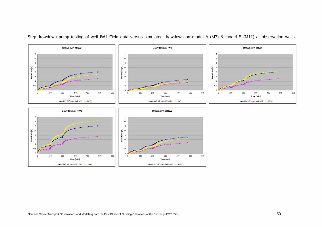
Flow and Solute Transport Observations and Modelling from the First Phase of Flushing Operations at the Salisbury ASTR Site 50
Step-drawdown pump testing of well IW1 Field data versus simulated drawdown on model A (M7) & model B (M11) at observation wells
Drawdown at IW2
0
0.5
1
1.5
2
2.5
3
3.5
4
0 100 200 300 400 500 600
Time [min]
Draw
dow
n [m
]
IW2 M7 IW2 M11 IW2
Drawdown at IW3
0
0.5
1
1.5
2
2.5
3
3.5
4
0 100 200 300 400 500 600
Time [min]
Draw
dow
n [m
]
IW3 M7 IW3 M11 IW3
Drawdown at IW4
0
0.5
1
1.5
2
2.5
3
3.5
4
0 100 200 300 400 500 600
Time [min]
Draw
dow
n [m
]
IW4 M7 IW4 M11 IW4
Drawdown at RW1
0
0.5
1
1.5
2
2.5
3
3.5
4
0 100 200 300 400 500 600
Time [min]
Draw
dow
n [m
]
RW1 M7 RW1 M11 RW1
Drawdown at RW2
0
0.5
1
1.5
2
2.5
3
3.5
4
0 100 200 300 400 500 600
Time [min]
Draw
dow
n [m
]
RW2 M7 RW2 M11 RW2