the supplemental poverty measure: 2013 - · pdf file · 2017-04-22issued october...

U.S. Department of Commerce Economics and Statistics Administration U.S. CENSUS BUREAU

census.gov

By Kathleen Short Issued October 2014 P60-251

Current Population Reports

The Supplemental Poverty Measure: 2013

INTRODUCTION

This is the fourth report describing the Supplemental Poverty Measure (SPM) released by the U.S. Census Bureau, with support from the Bureau of Labor Statistics (BLS). The SPM extends the official pov-erty measure by taking account of many of the government programs designed to assist low-income families and individuals that are not included in the current official poverty measure.

Concerns about the adequacy of the official measure culminated in a congressional appropriation in 1990 for an independent scientific study of the concepts, measure-ment methods, and information needed for a poverty measure. In response, the National Academy of Sciences (NAS) established the Panel on Poverty and Family Assistance, which released its report, Measur-ing Poverty: A New Approach, in the spring of 1995 (Citro and Michael, 1995). In March of 2010, an Inter-agency Technical Working Group on Developing a Supplemental Poverty Measure (ITWG) listed suggestions for a new measure that would sup-plement the current official measure

of poverty.1 The ITWG was charged with developing a set of initial starting points to permit the Census Bureau, in cooperation with the BLS, to produce the SPM that would be released along with the official measure each year. Their suggestions included:

• The SPM thresholds should represent a dollar amount spent on a basic set of goods that includes food, clothing, shelter, and utilities (FCSU), and a small additional amount to allow for other needs (e.g., household supplies, personal care, nonwork-related transportation). This threshold should be calculated with 5 years of expenditure data for family units with exactly two children using Consumer Expen-diture Survey data, and it should be adjusted (using a specified equivalence scale) to reflect the needs of different family types and geographic differences in housing costs. Adjustments to thresholds should be made over time to reflect real change in

1 For information, see ITWG, Observations From the Interagency Technical Working Group on Developing a Supplemental Poverty Measure (Interagency), March 2010, available at <www.census.gov/hhes/www/poverty /SPM_TWGObservations.pdf>, accessed September 2014.

expenditures on this basic bundle of goods at the 33rd percentile of the expenditure distribution. So far as possible with avail-able data, the calculation of FSCU should include any non-cash benefits that are counted on the resource side for food, shelter, clothing, and utilities. This is necessary for consistency of the threshold and resource definitions.

• The SPM family unit resources should be defined as the value of cash income from all sources, plus the value of noncash benefits that are available to buy the basic bundle of goods (FCSU) minus necessary expenses for critical goods and services not included in the thresholds. In-kind benefits include nutritional assistance, subsidized housing, and home energy assistance. Necessary expenses that must be subtracted include income taxes, Social Secu-rity payroll taxes, childcare and other work-related expenses, child support payments to another household, and contributions toward the cost of medical care, health insurance premiums, and other medical out-of-pocket costs.

The ITWG stated that the official poverty measure, as defined in

2 U.S. Census Bureau

Office of Management and Budget (OMB) Statistical Policy Directive No. 14, will not be replaced by the SPM. They noted that the official measure is sometimes identified in legislation regarding program eligibility and funding distribution, while the SPM will not be used in this way. The SPM is designed to provide information on aggre-gate levels of economic need at a national level or within large subpopulations or areas and, as such, the SPM will be an additional macroeconomic statistic providing further understanding of economic conditions and trends.

This report presents updated esti-mates of the prevalence of poverty in the United States, overall and for selected demographic groups, using the official measure and the SPM. Section one presents differ-ences between the official poverty measure and the SPM. Comparing the two measures sheds light on the effects of noncash benefits, taxes, and other nondiscretionary expenses on measured economic well-being. The distribution of income-to-poverty threshold ratios and poverty rates by state are

estimated and compared for the two measures. The second sec-tion of the report examines the SPM itself. Effects of benefits and expenses on SPM rates are explic-itly examined, and SPM estimates for 2013 are compared with the 2012 figures to assess changes in SPM rates from the previous year. SPM rates for the 5 years for which there are comparable estimates, 2009 to 2013, are also shown.

POVERTY ESTIMATES FOR 2013: OFFICIAL AND SPM

The measures presented in this study use the 2014 Current Popu-lation Survey Annual Social and Economic Supplement (CPS ASEC) income information that refers to calendar year 2013 to estimate SPM

resources.2 These are the same data used for the preparation of official

2 The data in this report are from the 2010 to 2014 Current Population Survey Annual Social and Economic Supplement (CPS ASEC). The estimates in this paper (which may be shown in text, figures, and tables) are based on responses from a sample of the population and may differ from actual values because of sampling variability or other factors. As a result, apparent differences between the estimates for two or more groups may not be statistically significant. All comparative state-ments have undergone statistical testing and are significant at the 90 percent confidence level unless otherwise noted. Standard errors were calculated using replicate weights. Further information about the source and accuracy of the estimates is available at <www.census.gov/hhes/www/p60-243sa .pdf>, <www.census.gov/hhes/www /p60-245sa.pdf>, and <ftp://ftp2.census .gov/library/publications/2014/demo /p60-249sa.pdf>, accessed September 2014. The 2014 CPS ASEC included redesigned questions for income and health insurance coverage. All of the approximately 98,000 addresses were eligible to receive the improved set of health insurance coverage items. The redesigned income questions were implemented using a split panel design. Approximately 68,000 addresses were selected to receive a set of income ques-tions similar to those used in the 2013 CPS ASEC. The remaining 30,000 addresses were selected to receive the redesigned income questions. The source of data for this report is the portion of the CPS ASEC sample which received the income questions consistent with the 2013 CPS ASEC, approximately 68,000 addresses. Estimates published in this report and the corresponding income and poverty detailed tables available on the Internet may vary from estimates based on the full sample.

Poverty Measure Concepts: Official and Supplemental

Official Poverty Measure Supplemental Poverty Measure

Measurement Units

Families and unrelated individuals

All related individuals who live at the same address, and any coresident unrelated children who are cared for by the family (such as foster children) and any cohabiters and their relatives

Poverty Threshold

Three times the cost of a minimum food diet in 1963

The mean of the 30th to 36th percentile of expenditures on food, clothing, shelter, and utilities (FCSU) of consumer units with exactly two children multiplied by 1.2

Threshold Adjustments

Vary by family size, composition, and age of householder

Geographic adjustments for differences in housing costs by tenure and a three-parameter equivalence scale for family size and composition

Updating Thresholds

Consumer Price Index: all items

Five-year moving average of expenditures on FCSU

Resource Measure

Gross before-tax cash income

Sum of cash income, plus noncash benefits that families can use to meet their FCSU needs, minus taxes (or plus tax credits), minus work expenses, minus out-of-pocket medical expenses and child support paid to another household

U.S. Census Bureau 3

poverty statistics and reported in DeNavas-Walt and Proctor (2014).3 The SPM thresholds for 2013 are based on out-of-pocket spending on basic needs (FCSU).4 Thresholds use 5 years of quarterly data from the Consumer Expendi-ture Survey (CE); the thresholds are produced at the BLS.5, 6

3 The official thresholds are used for the official poverty estimates presented here, however, unlike the official estimates, unrelated individuals under the age of 15 are included in the universe. Since the CPS ASEC does not ask income questions for individu-als under age 15, they are excluded from the universe for official poverty calculations. For the official poverty estimates shown in this report, all unrelated individuals under age 15 are included and presumed to be in poverty. For the SPM, they are assumed to share resources with the household reference person.

4 See appendix for description of thresh-old calculation.

5 Bureau of Labor Statistics, Experimental Poverty Measure Web site, <www.bls.gov/pir /spmhome.htm>, accessed September 2014.

6 See <www.bls.gov/cex/anthology08 /csxanth2.pdf> or <www.bls.gov/cex /anthology08/csxanth3.pdf> for information on the CE, accessed September 2014.

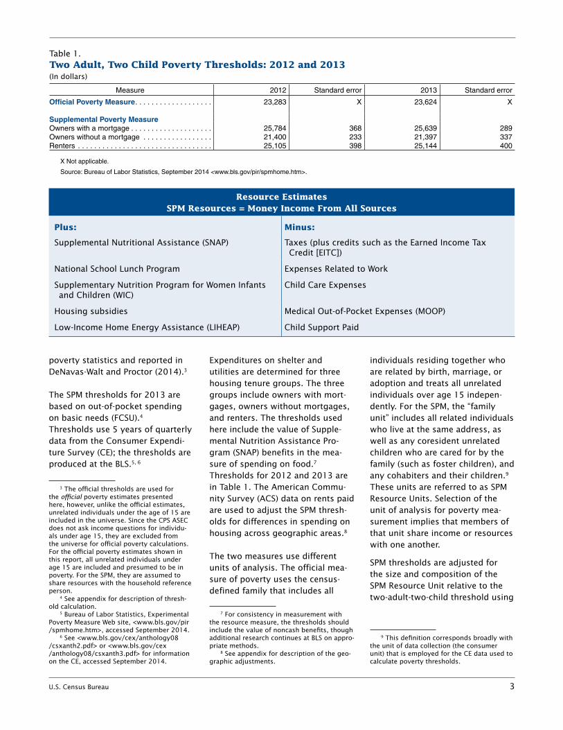
Expenditures on shelter and utilities are determined for three housing tenure groups. The three groups include owners with mort-gages, owners without mortgages, and renters. The thresholds used here include the value of Supple-mental Nutrition Assistance Pro-gram (SNAP) benefits in the mea-sure of spending on food.7 Thresholds for 2012 and 2013 are in Table 1. The American Commu-nity Survey (ACS) data on rents paid are used to adjust the SPM thresh-olds for differences in spending on housing across geographic areas.8

The two measures use different units of analysis. The official mea-sure of poverty uses the census-defined family that includes all

7 For consistency in measurement with the resource measure, the thresholds should include the value of noncash benefits, though additional research continues at BLS on appro-priate methods.

8 See appendix for description of the geo-graphic adjustments.

individuals residing together who are related by birth, marriage, or adoption and treats all unrelated individuals over age 15 indepen-dently. For the SPM, the “family unit” includes all related individuals who live at the same address, as well as any coresident unrelated children who are cared for by the family (such as foster children), and any cohabiters and their children.9 These units are referred to as SPM Resource Units. Selection of the unit of analysis for poverty mea-surement implies that members of that unit share income or resources with one another.

SPM thresholds are adjusted for the size and composition of the SPM Resource Unit relative to the two-adult-two-child threshold using

9 This definition corresponds broadly with the unit of data collection (the consumer unit) that is employed for the CE data used to calculate poverty thresholds.

Table 1.Two Adult, Two Child Poverty Thresholds: 2012 and 2013(In dollars)

Measure 2012 Standard error 2013 Standard error

Official Poverty Measure . . . . . . . . . . . . . . . . . . . 23,283 X 23,624 X

Supplemental Poverty Measure Owners with a mortgage . . . . . . . . . . . . . . . . . . . . 25,784 368 25,639 289 Owners without a mortgage . . . . . . . . . . . . . . . . . 21,400 233 21,397 337 Renters . . . . . . . . . . . . . . . . . . . . . . . . . . . . . . . . . 25,105 398 25,144 400

X Not applicable .

Source: Bureau of Labor Statistics, September 2014 <www .bls .gov/pir/spmhome .htm> .

Resource EstimatesSPM Resources = Money Income From All Sources

Plus: Minus:

Supplemental Nutritional Assistance (SNAP) Taxes (plus credits such as the Earned Income Tax Credit [EITC])

National School Lunch Program Expenses Related to Work

Supplementary Nutrition Program for Women Infants and Children (WIC)

Child Care Expenses

Housing subsidies Medical Out-of-Pocket Expenses (MOOP)

Low-Income Home Energy Assistance (LIHEAP) Child Support Paid


an equivalence scale.10 The official measure adjusts thresholds based on family size, number of children and adults, as well as whether or not the householder is aged 65 or over. The official poverty threshold for a two-adult-two-child family was $23,624 in 2013. The SPM thresholds vary by housing tenure and are higher for owners with mortgages and renters than the official threshold. These two groups comprise about 76 percent of the total population. The offi-cial threshold increased by $341 between 2012 and 2013. None of the SPM thresholds changed signifi-cantly between 2012 and 2013.

SPM resources are estimated as the sum of cash income plus any fed-eral government noncash benefits that families can use to meet their FCSU needs and minus taxes (plus tax credits), work expenses, and out-of-pocket medical expenses. The text box summarizes the addi-tions and subtractions for the SPM; descriptions are in the appendix.

POVERTY RATES: OFFICIAL AND SPM

Figure 1 shows poverty rates using the two measures for the total population and for three age groups: under 18 years, 18 to 64 years, and 65 years and over. Table 2 shows rates for a variety of selected demographic groups. The percent of the population that was poor using the official measure for 2013 was 14.5 percent (DeNavas-Walt and Proctor, 2014). For this study, including unrelated individu-als under age 15 in the universe, the official poverty rate was 14.6 percent.11 The SPM yields a rate

10 See appendix for description of the three-parameter scale.

11 The 14.5 and 14.6 rates are not statisti-cally different.

of 15.5 percent for 2013. While, as noted, SPM poverty thresholds are generally higher than official thresholds, other parts of the mea-sure also contribute to differences in the estimated prevalence of poverty in the United States.

In 2013, 48.7 million were poor using the SPM definition of poverty, more than the 45.8 million using the official definition of poverty with our universe. For most groups, SPM rates were higher than the offi-cial poverty rates. Compared with the official measure, the SPM shows lower poverty rates for children, individuals included in new SPM Resource Units, Blacks, renters, those living outside metropolitan areas, those covered by only public health insurance, and individuals with a work disability. Most other groups had higher poverty rates using the SPM, rather than the

official measure. Official and SPM poverty rates for females, people in female householder units, native-born citizens, residents of the South or the Midwest, and those not working at least 1 week were not statistically different. Note that poverty rates for those 65 years and over were higher under the SPM compared with the official measure. This partially reflects that the official thresholds are set lower for families with householders in this age group, while the SPM thresholds do not vary by age.12

Distribution of Income-to-Poverty Threshold Ratios: Official and SPM

Comparing the distribution of gross cash income with that of SPM

12 For more information about the SPM and the aged population, see Bridges and Gesumaria (2014).

Figure 1.Poverty Rates Using Two Measures for Total Population and by Age Group: 2013

0

5

10

15

20

25

65 yearsand older

18 to 64years

Under18 years

Allpeople

* Includes unrelated individuals under the age of 15.Source: U.S. Census Bureau, Current Population Survey, 2014 Annual Social and Economic Supplement.

Official*SPM

Percent


Table 2.Number and Percentage of People in Poverty by Different Poverty Measures: 2013—Con.(Data are based on the CPS ASEC sample of 68,000 addresses.1 Numbers in thousands, confidence intervals [C.I.] in thousands or percentage points as appropriate. People as of March of the following year. For information on confidentiality protection, sampling error, nonsampling error, and definitions, see ftp://ftp2.census.gov/programs-surveys/cps/techdocs/cpsmar14.pdf)

CharacteristicNum-ber**

(in thou-sands)

Official** SPM

DifferenceNumber Percent Number Percent

Esti-mate

90 percent C .I .† (±)

Esti-mate


Esti-mate


Esti-mate

90 percent C .I .† (±) Number Percent

All people . . . . . . . . . . . . . . . . 313,395 45,748 1,013 14 .6 0 .3 48,671 1,051 15 .5 0 .3 *2,923 *0 .9

SexMale . . . . . . . . . . . . . . . . . . . . . . . . . . 153,596 20,355 571 13 .3 0 .4 22,839 593 14 .9 0 .4 *2,484 *1 .6Female . . . . . . . . . . . . . . . . . . . . . . . . 159,799 25,393 571 15 .9 0 .4 25,832 581 16 .2 0 .4 439 0 .3

AgeUnder 18 years . . . . . . . . . . . . . . . . . 74,055 15,089 453 20 .4 0 .6 12,177 388 16 .4 0 .5 *–2,912 *–3 .918 to 64 years . . . . . . . . . . . . . . . . . . 194,833 26,429 648 13 .6 0 .3 29,987 700 15 .4 0 .4 *3,558 *1 .865 years and older . . . . . . . . . . . . . . . 44,508 4,231 227 9 .5 0 .5 6,507 271 14 .6 0 .6 *2,276 *5 .1

Type of UnitMarried couple . . . . . . . . . . . . . . . . . . 188,571 12,630 627 6 .7 0 .3 17,855 709 9 .5 0 .4 *5,226 *2 .8Female householder . . . . . . . . . . . . . 62,924 17,998 630 28 .6 0 .9 17,959 652 28 .5 0 .9 –39 –0 .1Male householder . . . . . . . . . . . . . . . 33,947 6,357 334 18 .7 0 .9 7,853 394 23 .1 1 .1 *1,496 *4 .4New SPM unit . . . . . . . . . . . . . . . . . . 27,953 8,764 427 31 .4 1 .3 5,004 379 17 .9 1 .3 *–3,760 *–13 .5

Race2 and Hispanic OriginWhite . . . . . . . . . . . . . . . . . . . . . . . . 243,399 30,250 815 12 .4 0 .3 33,445 818 13 .7 0 .3 *3,195 *1 .3 White, not Hispanic . . . . . . . . . . . . 195,399 19,027 723 9 .7 0 .4 20,946 668 10 .7 0 .3 *1,919 *1 .0Black . . . . . . . . . . . . . . . . . . . . . . . . . 40,671 11,097 507 27 .3 1 .3 10,056 498 24 .7 1 .2 *–1,041 *–2 .6Asian . . . . . . . . . . . . . . . . . . . . . . . . . 17,070 1,792 176 10 .5 1 .0 2,800 260 16 .4 1 .5 *1,008 *5 .9Hispanic (any race) . . . . . . . . . . . . . . 54,253 12,853 512 23 .7 0 .9 14,085 556 26 .0 1 .0 *1,232 *2 .3

NativityNative born . . . . . . . . . . . . . . . . . . . . 272,387 38,339 945 14 .1 0 .3 38,928 949 14 .3 0 .3 589 0 .2Foreign born . . . . . . . . . . . . . . . . . . . 41,009 7,409 372 18 .1 0 .8 9,743 427 23 .8 0 .9 *2,334 *5 .7 Naturalized citizen . . . . . . . . . . . . . 19,150 2,428 172 12 .7 0 .9 3,356 204 17 .5 1 .0 *928 *4 .8Not a citizen . . . . . . . . . . . . . . . . . . . . 21,859 4,981 311 22 .8 1 .2 6,387 366 29 .2 1 .3 *1,406 *6 .4

TenureOwner . . . . . . . . . . . . . . . . . . . . . . . . 208,717 16,127 734 7 .7 0 .3 20,504 761 9 .8 0 .4 *4,377 *2 .1 Owner/mortgage . . . . . . . . . . . . . . 136,059 7,739 479 5 .7 0 .4 11,267 569 8 .3 0 .4 *3,528 *2 .6 Owner/no mortgage/rent free . . . . . 75,999 9,254 486 12 .2 0 .5 9,970 524 13 .1 0 .6 *716 *0 .9Renter . . . . . . . . . . . . . . . . . . . . . . . . 101,338 28,755 876 28 .4 0 .7 27,434 855 27 .1 0 .7 *–1,321 *–1 .3

ResidenceInside metropolitan statistical areas . . . . . . . . . . . . . . . . . . . . . . . . . 266,259 38,089 1,006 14 .3 0 .3 42,452 1,052 15 .9 0 .4 *4,362 *1 .6 Inside principal cities . . . . . . . . . . . 102,295 19,676 845 19 .2 0 .7 20,516 760 20 .1 0 .6 *840 *0 .8 Outside principal cities . . . . . . . . . . 163,963 18,413 746 11 .2 0 .4 21,936 819 13 .4 0 .4 *3,523 *2 .1Outside metropolitan statistical areas3 . . . . . . . . . . . . . . . . . . . . . . . . 47,137 7,659 675 16 .2 1 .0 6,220 586 13 .2 0 .9 *–1,439 *–3 .1

RegionNortheast . . . . . . . . . . . . . . . . . . . . . . 55,566 7,134 442 12 .8 0 .8 7,947 490 14 .3 0 .9 *813 *1 .5Midwest . . . . . . . . . . . . . . . . . . . . . . . 66,872 8,677 432 13 .0 0 .7 8,351 416 12 .5 0 .6 –326 –0 .5South . . . . . . . . . . . . . . . . . . . . . . . . . 117,109 19,018 708 16 .2 0 .6 18,565 705 15 .9 0 .6 –454 –0 .4West . . . . . . . . . . . . . . . . . . . . . . . . . 73,849 10,919 433 14 .8 0 .6 13,809 495 18 .7 0 .7 *2,890 *3 .9

Health Insurance CoverageWith private insurance . . . . . . . . . . . . 201,064 10,440 461 5 .2 0 .2 16,439 604 8 .2 0 .3 *5,999 *3 .0With public, no private insurance . . . . 70,378 23,996 776 34 .1 0 .9 20,032 681 28 .5 0 .8 *–3,964 *–5 .6Not insured . . . . . . . . . . . . . . . . . . . . 41,953 11,313 431 27 .0 0 .9 12,201 468 29 .1 1 .0 *888 *2 .1

See footnotes at end of table .


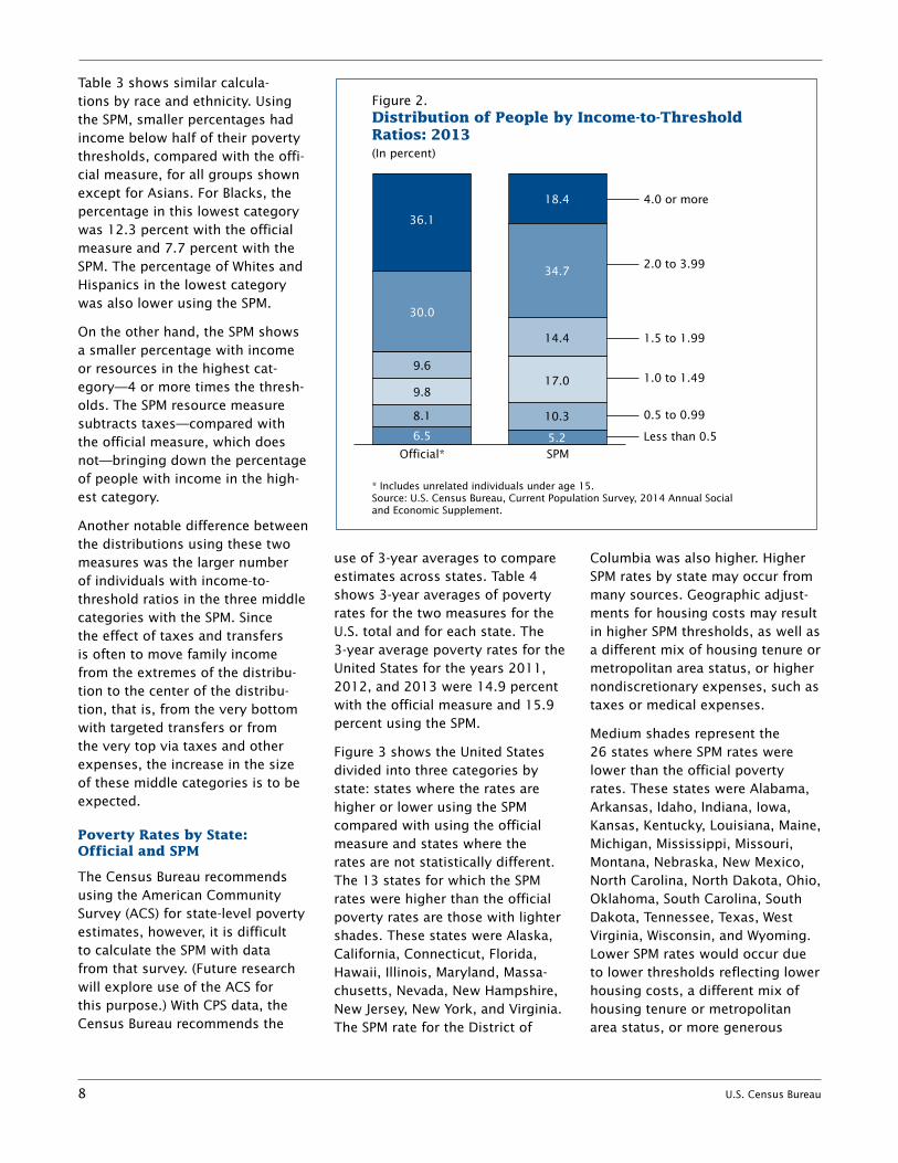
resources also allows an examina-tion of the effect of taxes and non-cash transfers on SPM rates. Table 3 shows the distribution of income-to-poverty threshold ratios for various groups. Dividing income by the respective poverty threshold controls income by unit size and composition. Figure 2 shows the percent distribution of income-to-threshold ratio categories for all people.

In general, the comparison sug-gests that a smaller percentage of the population was in the lowest category of the distribution using

the SPM. For most groups, includ-ing targeted noncash benefits reduced the percentage of the population in the lowest category—those with income below half their poverty threshold. This was true for the age groups shown in Table 3, except for those over age 64. They showed a higher percentage below half of the poverty line with the SPM: 4.8 percent compared to 2.7 percent with the official measure. As shown earlier, many of the non-cash benefits included in the SPM are not targeted to this population. Further, many transfers received by

this group are in cash, especially Social Security payments, and are captured in the official measure, as well as the SPM. Note that the per-centage of the 65 years and over age group with cash income below half their threshold was lower than that of other age groups under the official measure (2.7 percent), while the percentage for children was higher (9.3 percent). Subtract-ing MOOP and other expenses and adding noncash benefits in the SPM narrowed the differences across the three age groups.

Table 2.Number and Percentage of People in Poverty by Different Poverty Measures: 2013—Con.(Data are based on the CPS ASEC sample of 68,000 addresses.1 Numbers in thousands, confidence intervals [C.I.] in thousands or percentage points as appropriate. People as of March of the following year. For information on confidentiality protection, sampling error, nonsampling error, and definitions, see ftp://ftp2.census.gov/programs-surveys/cps/techdocs/cpsmar14.pdf)

CharacteristicNum-ber**

(in thou-sands)

Official** SPM

DifferenceNumber Percent Number Percent

Esti-mate


Esti-mate


Esti-mate


Esti-mate

90 percent C .I .† (±) Number Percent

Work Experience Total, 18 to 64 years . . . . . . . . 194,833 26,429 648 13 .6 0 .3 29,987 700 15 .4 0 .4 *3,558 *1 .8All workers . . . . . . . . . . . . . . . . . . . . . 146,252 10,736 347 7 .3 0 .2 14,357 447 9 .8 0 .3 *3,621 *2 .5Worked full-time, year-round . . . . . . . 100,855 2,771 155 2 .7 0 .2 5,479 214 5 .4 0 .2 *2,708 *2 .7Less than full-time, year-round . . . . . 45,397 7,965 322 17 .5 0 .6 8,878 353 19 .6 0 .7 *913 *2 .0Did not work at least 1 week . . . . . . . 48,581 15,693 515 32 .3 0 .9 15,630 504 32 .2 0 .8 –63 –0 .1

Disability Status4

Total, 18 to 64 years . . . . . . . . 194,833 26,429 648 13 .6 0 .3 29,987 700 15 .4 0 .4 *3,558 *1 .8With a disability . . . . . . . . . . . . . . . . . 15,098 4,352 233 28 .8 1 .2 4,126 235 27 .3 1 .2 *–226 *–1 .5With no disability . . . . . . . . . . . . . . . . 178,761 22,023 567 12 .3 0 .3 25,799 649 14 .4 0 .4 *3,776 *2 .1

* An asterisk preceding an estimate indicates change is statistically different from zero at the 90 percent confidence level .

** Includes unrelated individuals under the age of 15 .† A 90 percent confidence interval is a measure of an estimate’s variability . The larger the confidence interval in relation to the size of the estimate, the less

reliable the estimate . Confidence intervals shown in this table are based on standard errors calculated using replicate weights . For more information see “Standard Errors and Their Use” at <ftp://ftp2 .census .gov/library/publications/2014/demo/p60-249sa .pdf> .

1 The 2014 CPS ASEC included redesigned questions for income and health insurance coverage . All of the approximately 98,000 addresses were eligible to receive the redesigned set of health insurance coverage questions . The redesigned income questions were implemented to a subsample of these 98,000 addresses using a probability split panel design . Approximately 68,000 addresses were eligible to receive a set of income questions similar to those used in the 2013 CPS ASEC and the remaining 30,000 addresses were eligible to receive the redesigned income questions . The source of the 2013 data for this table is the portion of the CPS ASEC sample which received the income questions consistent with the 2013 CPS ASEC, approximately 68,000 addresses .

2 Federal surveys give respondents the option of reporting more than one race . Therefore, two basic ways of defining a race group are possible . A group such as Asian may be defined as those who reported Asian and no other race (the race-alone or single-race concept) or as those who reported Asian regardless of whether they also reported another race (the race-alone-or-in-combination concept) . This table shows data using the first approach (race alone) . The use of the single-race population does not imply that it is the preferred method of presenting or analyzing data . The Census Bureau uses a variety of approaches . Information on people who reported more than one race, such as White and American Indian and Alaska Native or Asian and Black or African American, is available from Census 2010 through American FactFinder . About 2 .9 percent of people reported more than one race in Census 2010 . Data for American Indians and Alaska Natives, Native Hawaiians and Other Pacific Islanders, and those reporting two or more races are not shown separately .

3 The “Outside metropolitan statistical areas” category includes both micropolitan statistical areas and territory outside of metropolitan and micropolitan statisti-cal areas . For more information, see “About Metropolitan and Micropolitan Statistical Areas” at <www .census .gov/population/metro> .

4 The sum of those with and without a disability does not equal the total because disability status is not defined for individuals in the Armed Forces .

Source: U .S . Census Bureau, Current Population Survey, 2014 Annual Social and Economic Supplement .


Table 3.Percentage of People by Ratio of Income/Resources to Poverty Threshold: 2013(Data are based on the CPS ASEC sample of 68,000 addresses.1 Numbers in thousands, confidence intervals [C.I.] in thousands or percentage points as appropriate. People as of March of the following year. For information on confidentiality protection, sampling error, nonsampling error, and definitions, see ftp://ftp2.census.gov/programs-surveys/cps/techdocs/cpsmar14.pdf)

CharacteristicLess than 0 .5


0 .5 to 0 .99


1 .0 to 1 .49


1 .5 to 1 .99


2 .0 to 3 .99


4 .0 or more


OFFICIAL*

All people . . . . . . . . . . . . . . 6 .5 0 .2 8 .1 0 .3 9 .8 0 .2 9 .6 0 .3 30 .0 0 .4 36 .1 0 .5

AgeUnder 18 years . . . . . . . . . . . . . . . 9 .3 0 .4 11 .0 0 .6 12 .1 0 .5 10 .4 0 .4 29 .1 0 .7 28 .0 0 .618 to 64 years . . . . . . . . . . . . . . . . 6 .2 0 .2 7 .3 0 .2 8 .5 0 .2 8 .6 0 .3 29 .6 0 .4 39 .7 0 .565 years and older . . . . . . . . . . . . . 2 .7 0 .3 6 .8 0 .4 11 .5 0 .5 12 .1 0 .6 33 .0 0 .9 33 .8 1 .0

Race2 and Hispanic OriginWhite . . . . . . . . . . . . . . . . . . . . . . 5 .4 0 .2 7 .0 0 .3 9 .1 0 .3 9 .5 0 .3 30 .5 0 .5 38 .4 0 .5 White, not Hispanic . . . . . . . . . . 4 .4 0 .2 5 .3 0 .2 7 .4 0 .3 8 .5 0 .3 30 .8 0 .6 43 .5 0 .6Black . . . . . . . . . . . . . . . . . . . . . . . 12 .3 0 .8 14 .9 1 .0 13 .5 0 .9 10 .0 0 .7 27 .1 1 .1 22 .1 1 .1Asian . . . . . . . . . . . . . . . . . . . . . . . 5 .2 0 .7 5 .3 0 .8 8 .7 1 .2 8 .9 1 .1 29 .6 1 .9 42 .3 2 .0Hispanic (any race) . . . . . . . . . . . . 9 .6 0 .6 14 .1 0 .8 15 .8 0 .8 13 .6 0 .7 29 .1 1 .0 17 .8 0 .8

SPM

All people . . . . . . . . . . . . . . 5 .2 0 .2 10 .3 0 .3 17 .0 0 .3 14 .4 0 .3 34 .7 0 .4 18 .4 0 .4

AgeUnder 18 years . . . . . . . . . . . . . . . 4 .4 0 .3 12 .0 0 .5 21 .5 0 .6 16 .7 0 .5 33 .2 0 .6 12 .2 0 .418 to 64 years . . . . . . . . . . . . . . . . 5 .6 0 .2 9 .8 0 .3 15 .2 0 .4 13 .8 0 .3 35 .5 0 .4 20 .2 0 .565 years and older . . . . . . . . . . . . . 4 .8 0 .4 9 .8 0 .5 17 .2 0 .7 13 .3 0 .6 33 .9 0 .9 20 .9 0 .8

Race2 and Hispanic OriginWhite . . . . . . . . . . . . . . . . . . . . . . 4 .7 0 .2 9 .0 0 .3 15 .5 0 .3 14 .0 0 .4 36 .2 0 .5 20 .5 0 .4 White, not Hispanic . . . . . . . . . . 4 .1 0 .2 6 .6 0 .3 12 .6 0 .4 13 .4 0 .4 39 .3 0 .5 24 .0 0 .5Black . . . . . . . . . . . . . . . . . . . . . . . 7 .7 0 .7 17 .0 1 .0 24 .2 1 .1 16 .1 0 .9 26 .6 1 .2 8 .5 0 .6Asian . . . . . . . . . . . . . . . . . . . . . . . 6 .0 0 .8 10 .4 1 .3 16 .9 1 .5 14 .4 1 .4 35 .1 1 .9 17 .1 1 .4Hispanic (any race) . . . . . . . . . . . . 7 .0 0 .5 18 .9 0 .9 27 .5 0 .9 16 .3 0 .8 24 .0 1 .0 6 .2 0 .4

* Includes unrelated individuals under the age of 15 .† A 90 percent confidence interval is a measure of an estimate’s variability . The larger the confidence interval in relation to the size of the estimate, the less






Table 3 shows similar calcula-tions by race and ethnicity. Using the SPM, smaller percentages had income below half of their poverty thresholds, compared with the offi-cial measure, for all groups shown except for Asians. For Blacks, the percentage in this lowest category was 12.3 percent with the official measure and 7.7 percent with the SPM. The percentage of Whites and Hispanics in the lowest category was also lower using the SPM.

On the other hand, the SPM shows a smaller percentage with income or resources in the highest cat-egory—4 or more times the thresh-olds. The SPM resource measure subtracts taxes—compared with the official measure, which does not—bringing down the percentage of people with income in the high-est category.

Another notable difference between the distributions using these two measures was the larger number of individuals with income-to-threshold ratios in the three middle categories with the SPM. Since the effect of taxes and transfers is often to move family income from the extremes of the distribu-tion to the center of the distribu-tion, that is, from the very bottom with targeted transfers or from the very top via taxes and other expenses, the increase in the size of these middle categories is to be expected.

Poverty Rates by State: Official and SPM

The Census Bureau recommends using the American Community Survey (ACS) for state-level poverty estimates, however, it is difficult to calculate the SPM with data from that survey. (Future research will explore use of the ACS for this purpose.) With CPS data, the Census Bureau recommends the

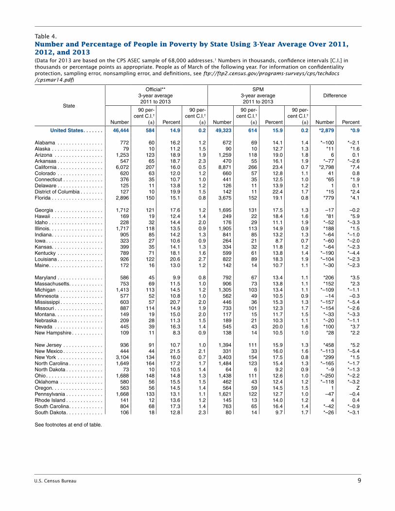
use of 3-year averages to compare estimates across states. Table 4 shows 3-year averages of poverty rates for the two measures for the U.S. total and for each state. The 3-year average poverty rates for the United States for the years 2011, 2012, and 2013 were 14.9 percent with the official measure and 15.9 percent using the SPM.

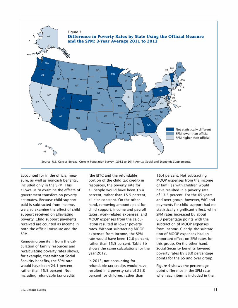
Figure 3 shows the United States divided into three categories by state: states where the rates are higher or lower using the SPM compared with using the official measure and states where the rates are not statistically different. The 13 states for which the SPM rates were higher than the official poverty rates are those with lighter shades. These states were Alaska, California, Connecticut, Florida, Hawaii, Illinois, Maryland, Massa-chusetts, Nevada, New Hampshire, New Jersey, New York, and Virginia. The SPM rate for the District of

Columbia was also higher. Higher SPM rates by state may occur from many sources. Geographic adjust-ments for housing costs may result in higher SPM thresholds, as well as a different mix of housing tenure or metropolitan area status, or higher nondiscretionary expenses, such as taxes or medical expenses.

Medium shades represent the 26 states where SPM rates were lower than the official poverty rates. These states were Alabama, Arkansas, Idaho, Indiana, Iowa, Kansas, Kentucky, Louisiana, Maine, Michigan, Mississippi, Missouri, Montana, Nebraska, New Mexico, North Carolina, North Dakota, Ohio, Oklahoma, South Carolina, South Dakota, Tennessee, Texas, West Virginia, Wisconsin, and Wyoming. Lower SPM rates would occur due to lower thresholds reflecting lower housing costs, a different mix of housing tenure or metropolitan area status, or more generous

1.0 to 1.49

Figure 2.Distribution of People by Income-to-Threshold Ratios: 2013

* Includes unrelated individuals under age 15.Source: U.S. Census Bureau, Current Population Survey, 2014 Annual Social and Economic Supplement.

(In percent)

SPMOfficial*

30.0

36.1

9.6

18.4

34.7

17.0

14.4

10.38.1

9.8

6.5 5.2

4.0 or more

2.0 to 3.99

1.5 to 1.99

0.5 to 0.99

Less than 0.5


Table 4.Number and Percentage of People in Poverty by State Using 3-Year Average Over 2011, 2012, and 2013—Con.(Data for 2013 are based on the CPS ASEC sample of 68,000 addresses.1 Numbers in thousands, confidence intervals [C.I.] in thousands or percentage points as appropriate. People as of March of the following year. For information on confidentiality protection, sampling error, nonsampling error, and definitions, see ftp://ftp2.census.gov/programs-surveys/cps/techdocs /cpsmar14.pdf)

State

Official**3-year average2011 to 2013

SPM3-year average2011 to 2013

Difference

Number

90 per-cent C .I .†

(±) Percent


(±) Number


(±) Percent


(±) Number Percent

United States . . . . . . . 46,444 584 14 .9 0 .2 49,323 614 15 .9 0 .2 *2,879 *0 .9

Alabama . . . . . . . . . . . . . . . . 772 60 16 .2 1 .2 672 69 14 .1 1 .4 *–100 *–2 .1Alaska . . . . . . . . . . . . . . . . . . 79 10 11 .2 1 .5 90 10 12 .7 1 .3 *11 *1 .6Arizona . . . . . . . . . . . . . . . . . 1,253 123 18 .9 1 .9 1,259 118 19 .0 1 .8 6 0 .1Arkansas . . . . . . . . . . . . . . . . 547 65 18 .7 2 .3 470 55 16 .1 1 .9 *–77 *–2 .6California . . . . . . . . . . . . . . . . 6,072 207 16 .0 0 .5 8,871 266 23 .4 0 .7 *2,798 *7 .4Colorado . . . . . . . . . . . . . . . . 620 63 12 .0 1 .2 660 57 12 .8 1 .1 41 0 .8Connecticut . . . . . . . . . . . . . . 376 35 10 .7 1 .0 441 35 12 .5 1 .0 *65 *1 .9Delaware . . . . . . . . . . . . . . . . 125 11 13 .8 1 .2 126 11 13 .9 1 .2 1 0 .1District of Columbia . . . . . . . . 127 10 19 .9 1 .5 142 11 22 .4 1 .7 *15 *2 .4Florida . . . . . . . . . . . . . . . . . . 2,896 150 15 .1 0 .8 3,675 152 19 .1 0 .8 *779 *4 .1

Georgia . . . . . . . . . . . . . . . . . 1,712 121 17 .6 1 .2 1,695 131 17 .5 1 .3 –17 –0 .2Hawaii . . . . . . . . . . . . . . . . . . 169 19 12 .4 1 .4 249 22 18 .4 1 .6 *81 *5 .9Idaho . . . . . . . . . . . . . . . . . . . 228 32 14 .4 2 .0 176 29 11 .1 1 .9 *–52 *–3 .3Illinois . . . . . . . . . . . . . . . . . . . 1,717 118 13 .5 0 .9 1,905 113 14 .9 0 .9 *188 *1 .5Indiana . . . . . . . . . . . . . . . . . . 905 85 14 .2 1 .3 841 85 13 .2 1 .3 *–64 *–1 .0Iowa . . . . . . . . . . . . . . . . . . . . 323 27 10 .6 0 .9 264 21 8 .7 0 .7 *–60 *–2 .0Kansas . . . . . . . . . . . . . . . . . . 399 35 14 .1 1 .3 334 32 11 .8 1 .2 *–64 *–2 .3Kentucky . . . . . . . . . . . . . . . . 789 71 18 .1 1 .6 599 61 13 .8 1 .4 *–190 *–4 .4Louisiana . . . . . . . . . . . . . . . . 926 122 20 .6 2 .7 822 89 18 .3 1 .9 *–104 *–2 .3Maine . . . . . . . . . . . . . . . . . . . 172 16 13 .0 1 .2 142 14 10 .7 1 .1 *–30 *–2 .3

Maryland . . . . . . . . . . . . . . . . 586 45 9 .9 0 .8 792 67 13 .4 1 .1 *206 *3 .5Massachusetts . . . . . . . . . . . . 753 69 11 .5 1 .0 906 73 13 .8 1 .1 *152 *2 .3Michigan . . . . . . . . . . . . . . . . 1,413 113 14 .5 1 .2 1,305 103 13 .4 1 .1 *–109 *–1 .1Minnesota . . . . . . . . . . . . . . . 577 52 10 .8 1 .0 562 49 10 .5 0 .9 –14 –0 .3Mississippi . . . . . . . . . . . . . . . 603 57 20 .7 2 .0 446 36 15 .3 1 .3 *–157 *–5 .4Missouri . . . . . . . . . . . . . . . . . 887 114 14 .9 1 .9 733 101 12 .3 1 .7 *–154 *–2 .6Montana . . . . . . . . . . . . . . . . . 149 19 15 .0 2 .0 117 15 11 .7 1 .5 *–33 *–3 .3Nebraska . . . . . . . . . . . . . . . . 209 28 11 .3 1 .5 189 21 10 .3 1 .1 *–20 *–1 .1Nevada . . . . . . . . . . . . . . . . . 445 39 16 .3 1 .4 545 43 20 .0 1 .6 *100 *3 .7New Hampshire . . . . . . . . . . . 109 11 8 .3 0 .9 138 14 10 .5 1 .0 *28 *2 .2

New Jersey . . . . . . . . . . . . . . 936 91 10 .7 1 .0 1,394 111 15 .9 1 .3 *458 *5 .2New Mexico . . . . . . . . . . . . . . 444 44 21 .5 2 .1 331 33 16 .0 1 .6 *–113 *–5 .4New York . . . . . . . . . . . . . . . . 3,104 134 16 .0 0 .7 3,403 154 17 .5 0 .8 *299 *1 .5North Carolina . . . . . . . . . . . . 1,649 164 17 .2 1 .7 1,484 123 15 .4 1 .3 *–165 *–1 .7North Dakota . . . . . . . . . . . . . 73 10 10 .5 1 .4 64 6 9 .2 0 .9 *–9 *–1 .3Ohio . . . . . . . . . . . . . . . . . . . . 1,688 148 14 .8 1 .3 1,438 111 12 .6 1 .0 *–250 *–2 .2Oklahoma . . . . . . . . . . . . . . . 580 56 15 .5 1 .5 462 43 12 .4 1 .2 *–118 *–3 .2Oregon . . . . . . . . . . . . . . . . . . 563 56 14 .5 1 .4 564 59 14 .5 1 .5 1 ZPennsylvania . . . . . . . . . . . . . 1,668 133 13 .1 1 .1 1,621 122 12 .7 1 .0 –47 –0 .4Rhode Island . . . . . . . . . . . . . 141 12 13 .6 1 .2 145 13 14 .0 1 .2 4 0 .4South Carolina . . . . . . . . . . . . 804 68 17 .3 1 .4 763 65 16 .4 1 .4 *–42 *–0 .9South Dakota . . . . . . . . . . . . . 106 18 12 .8 2 .3 80 14 9 .7 1 .7 *–26 *–3 .1



noncash benefits. Darker shades are those 11 states that were not statistically different under the two measures and include Arizona, Colorado, Delaware, Georgia, Minnesota, Oregon, Pennsylvania, Rhode Island, Utah, Vermont, and Washington. Details are in Table 4.

THE SUPPLEMENTAL POVERTY MEASURE

The Effect of Cash and Noncash Transfers, Taxes, and Other Nondiscretionary Expenses

The purpose of this section is to move away from comparing the SPM with the official measure and look only at the SPM. This exer-cise allows us to gauge the effects of taxes and transfers and other

necessary expenses using the SPM as the measure of economic well-being. The previous section char-acterized the poverty population using the SPM in comparison with the current official measure. This section examines in more detail the population defined as poor when using the SPM.

The official poverty measure takes account of cash benefits from the government, such as Social Security and Unemployment Insurance (UI) benefits, Supplemental Security Income (SSI), public assistance benefits, such as TANF, and work-ers’ compensation benefits, but does not take account of taxes or noncash benefits aimed at improv-ing the economic situation of the poor. Besides taking account

of cash benefits and necessary expenses, such as MOOP expenses and expenses related to work, the SPM includes taxes and noncash transfers. The important contribu-tion that the SPM provides is allow-ing us to gauge the effectiveness of tax credits and transfers in alleviat-ing poverty. We can also examine the effects of the nondiscretionary expenses such as work and MOOP expenses.

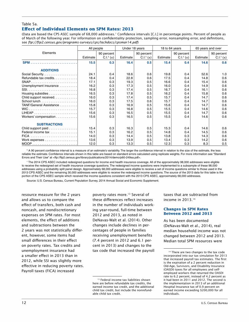
Table 5a shows the effect that vari-ous additions and subtractions had on the SPM rate in 2013, holding all else the same and assuming no behavioral changes. Additions and subtractions are shown for the total population and by three age groups. Additions shown in the table include cash benefits, also

Table 4.Number and Percentage of People in Poverty by State Using 3-Year Average Over 2011, 2012, and 2013—Con.(Data for 2013 are based on the CPS ASEC sample of 68,000 addresses.1 Numbers in thousands, confidence intervals [C.I.] in thousands or percentage points as appropriate. People as of March of the following year. For information on confidentiality protection, sampling error, nonsampling error, and definitions, see ftp://ftp2.census.gov/programs-surveys/cps/techdocs /cpsmar14.pdf)

State

Official**3-year average2011 to 2013

SPM3-year average2011 to 2013

Difference

Number


(±) Percent


(±) Number


(±) Percent


(±) Number Percent

Tennessee . . . . . . . . . . . . . . . 1,139 126 17 .8 2 .0 1,003 102 15 .6 1 .6 *–136 *–2 .1Texas . . . . . . . . . . . . . . . . . . . 4,484 233 17 .2 0 .9 4,143 218 15 .9 0 .8 *–341 *–1 .3Utah . . . . . . . . . . . . . . . . . . . . 289 39 10 .2 1 .4 315 50 11 .1 1 .8 25 0 .9Vermont . . . . . . . . . . . . . . . . . 66 6 10 .6 1 .0 60 6 9 .7 1 .0 –6 –0 .9Virginia . . . . . . . . . . . . . . . . . . 880 81 10 .9 1 .0 1,092 108 13 .6 1 .3 *211 *2 .6Washington . . . . . . . . . . . . . . 833 76 12 .2 1 .1 866 63 12 .6 0 .9 33 0 .5West Virginia . . . . . . . . . . . . . 317 52 17 .4 2 .7 240 36 13 .2 1 .9 *–77 *–4 .2Wisconsin . . . . . . . . . . . . . . . 680 64 12 .0 1 .1 635 60 11 .2 1 .1 *–45 *–0 .8Wyoming . . . . . . . . . . . . . . . . 63 7 10 .9 1 .3 55 6 9 .7 1 .1 *–7 *–1 .3

Z Represents or rounds to zero .

* An asterisk preceding an estimate indicates change is statistically different from zero at the 90 percent confidence level .

** Includes unrelated individuals under the age of 15 .† A 90 percent confidence interval is a measure of an estimate’s variability . The larger the confidence interval in relation to the size of the estimate, the less



Source: U .S . Census Bureau, Current Population Survey, 2012 to 2014 Annual Social and Economic Supplements .


accounted for in the official mea-sure, as well as noncash benefits, included only in the SPM. This allows us to examine the effects of government transfers on poverty estimates. Because child support paid is subtracted from income, we also examine the effect of child support received on alleviating poverty. Child support payments received are counted as income in both the official measure and the SPM.

Removing one item from the cal-culation of family resources and recalculating poverty rates shows, for example, that without Social Security benefits, the SPM rate would have been 24.1 percent, rather than 15.5 percent. Not including refundable tax credits

(the EITC and the refundable portion of the child tax credit) in resources, the poverty rate for all people would have been 18.4 percent, rather than 15.5 percent, all else constant. On the other hand, removing amounts paid for child support, income and payroll taxes, work-related expenses, and MOOP expenses from the calcu-lation resulted in lower poverty rates. Without subtracting MOOP expenses from income, the SPM rate would have been 12.0 percent, rather than 15.5 percent. Table 5b shows the same calculations for the year 2012.

In 2013, not accounting for refundable tax credits would have resulted in a poverty rate of 22.8 percent for children, rather than

16.4 percent. Not subtracting MOOP expenses from the income of families with children would have resulted in a poverty rate of 13.3 percent. For the 65 years and over group, however, WIC and payments for child support had no statistically significant effect, while SPM rates increased by about 6.3 percentage points with the subtraction of MOOP expenses from income. Clearly, the subtrac-tion of MOOP expenses had an important effect on SPM rates for this group. On the other hand, Social Security benefits lowered poverty rates by 38.0 percentage points for the 65 and over group.

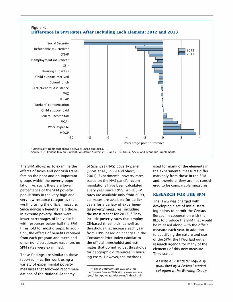
Figure 4 shows the percentage point difference in the SPM rate when each item is included in the

Figure 3.Difference in Poverty Rates by State Using the Official Measure and the SPM: 3-Year Average 2011 to 2013

Source: U.S. Census Bureau, Current Population Survey, 2012 to 2014 Annual Social and Economic Supplements.

MT

AK

NM

OR MN

KS

SD

ND

MO

WA

FL

IL IN

WI NY

PA

MI

OH

IA

ME

MA

CT

AZ

NV

TX

COCA

WY

UT

ID

NE

OK

GA

AR

AL

NC

MS

LA

TN

KY

VA

SC

WV

RI

DE MD

NJ

HI

VTNH

DC *

Not statistically differentSPM lower than officialSPM higher than official


resource measure for the 2 years and allows us to compare the effect of transfers, both cash and noncash, and nondiscretionary expenses on SPM rates. For most elements, the effect of additions and subtractions between the 2 years was not statistically differ-ent, however, some items had small differences in their effect on poverty rates. Tax credits and unemployment insurance had a smaller effect in 2013 than in 2012, while SSI was slightly more effective in reducing poverty rates. Payroll taxes (FICA) increased

poverty rates more.13 Several of these differences reflect increases in the number of individuals work-ing year-round, full-time between 2012 and 2013, as noted in DeNavas-Walt et al. (2014). Other changes include declines in per-centages of people in families receiving unemployment benefits (7.4 percent in 2012 and 6.1 per-cent in 2013) and changes to the tax code that increased the payroll

13 Federal income tax liabilities shown here are before refundable tax credits, the earned income tax credit, and the additional child tax credit, but include the nonrefund-able child tax credit.

taxes that are subtracted from income in 2013.14

Changes in SPM Rates Between 2012 and 2013

As has been documented (DeNavas-Walt et al., 2014), real median household income was not changed between 2012 and 2013. Median total SPM resources were

14 There are two changes to the tax code incorporated into our tax simulation for 2013 that increased payroll tax estimates. The first is the expiration of a 2 percent reduction in Old-Age, Survivors, and Disability Insurance (OASDI) taxes for all employees and self-employed workers that returned the OASDI rate to 6.2 percent, instead of 4.2 percent as it had been in 2011 and 2012. The second is the implementation in 2013 of an additional Hospital Insurance tax of 0.9 percent on earned income exceeding $200,000 for all individuals.

Table 5a.Effect of Individual Elements on SPM Rates: 2013(Data are based the CPS ASEC sample of 68,000 addresses.1 Confidence intervals [C.I.] in percentage points. Percent of people as of March of the following year. For information on confidentiality protection, sampling error, nonsampling error, and definitions, see ftp://ftp2.census.gov/programs-surveys/cps/techdocs/cpsmar14.pdf)

ElementsAll people Under 18 years 18 to 64 years 65 years and over

Estimate90 percent

C .I .† (±) Estimate90 percent



C .I .† (±)

SPM . . . . . . . . . . . . . . . . . . . . . . . . . . 15 .5 0 .3 16 .4 0 .5 15 .4 0 .4 14 .6 0 .6

ADDITIONSSocial Security . . . . . . . . . . . . . . . . . . . 24 .1 0 .4 18 .6 0 .6 19 .8 0 .4 52 .6 1 .0Refundable tax credits . . . . . . . . . . . . . 18 .4 0 .4 22 .8 0 .6 17 .5 0 .4 14 .8 0 .6SNAP . . . . . . . . . . . . . . . . . . . . . . . . . . 17 .1 0 .3 19 .3 0 .5 16 .6 0 .4 15 .4 0 .6Unemployment insurance . . . . . . . . . . 16 .2 0 .3 17 .3 0 .5 16 .0 0 .4 14 .9 0 .6SSI . . . . . . . . . . . . . . . . . . . . . . . . . . . . 16 .8 0 .3 17 .4 0 .5 16 .7 0 .4 16 .1 0 .6Housing subsidies . . . . . . . . . . . . . . . . 16 .5 0 .3 17 .8 0 .5 16 .2 0 .4 15 .8 0 .6Child support received . . . . . . . . . . . . . 16 .0 0 .3 17 .4 0 .5 15 .7 0 .4 14 .7 0 .6School lunch . . . . . . . . . . . . . . . . . . . . 16 .0 0 .3 17 .5 0 .6 15 .7 0 .4 14 .7 0 .6TANF/General Assistance . . . . . . . . . . 15 .8 0 .3 16 .9 0 .5 15 .6 0 .4 14 .7 0 .6WIC . . . . . . . . . . . . . . . . . . . . . . . . . . . 15 .7 0 .3 16 .8 0 .5 15 .5 0 .4 14 .6 0 .6LIHEAP . . . . . . . . . . . . . . . . . . . . . . . . 15 .6 0 .3 16 .5 0 .5 15 .5 0 .4 14 .7 0 .6Workers’ compensation . . . . . . . . . . . . 15 .6 0 .3 16 .5 0 .5 15 .5 0 .4 14 .6 0 .6

SUBTRACTIONSChild support paid . . . . . . . . . . . . . . . . 15 .4 0 .3 16 .3 0 .5 15 .3 0 .4 14 .6 0 .6Federal income tax . . . . . . . . . . . . . . . 15 .1 0 .3 16 .2 0 .5 14 .8 0 .4 14 .5 0 .6FICA . . . . . . . . . . . . . . . . . . . . . . . . . . 14 .0 0 .3 14 .4 0 .5 13 .8 0 .3 14 .3 0 .6Work expenses . . . . . . . . . . . . . . . . . . 13 .6 0 .3 13 .9 0 .5 13 .4 0 .3 14 .2 0 .6MOOP . . . . . . . . . . . . . . . . . . . . . . . . . 12 .0 0 .3 13 .3 0 .5 12 .3 0 .3 8 .3 0 .5

† A 90 percent confidence interval is a measure of an estimate’s variability . The larger the confidence interval in relation to the size of the estimate, the less reliable the estimate . Confidence intervals shown in this table are based on standard errors calculated using replicate weights . For more information see “Standard Errors and Their Use” at <ftp://ftp2 .census .gov/library/publications/2014/demo/p60-249sa .pdf> .




$37,295 for 2012 (in 2013 dollars) and $37,116 in 2013, not statisti-cally different. Despite increased official poverty thresholds, there was a decline in the official poverty rate. Both the official and the SPM rates declined by 0.5 percentage points between 2012 and 2013.

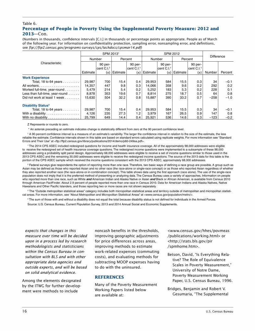
Table 6 shows SPM rates for 2012 and 2013, calculated in a compa-rable way for each year. In 2013, the percent poor using the SPM was 15.5 percent, and in 2012 that rate was 16.0 percent. While for most groups there were no changes in SPM rates across the 2 years, there were small increases for those with private health insurance and declines for those with public insur-ance and the uninsured. Changes to the 2014 CPS ASEC questionnaire about health insurance premiums and other out-of-pocket costs may

be reflected in the 2013 rates by health insurance status.15

SPM rates also declined for several groups including children, those in married-couple families, Hispan-ics, the foreign born, noncitizens, renters, and those residing inside principal cities or in the Northeast. There were declines in the official measure for most of these groups including females, children, those in married-couple families, Hispan-ics, the foreign born, and nonciti-zens (DeNavas-Walt et al., 2014). All other groups in Table 6 showed no change in SPM rates between 2012 and 2013.

Finally, we show the official mea-sure and the SPM over the 5 years for which we have estimates. Figure 5 shows the official measure

15 See Janicki (2014) and Smith and Medalia (2014) for more details on question-naire changes to the 2014 ASEC.

and the SPM across 4 years. Figure 6 shows the poverty rate using both measures for children and for those over 64 years.16

SUMMARY

This report provides estimates of the Supplemental Poverty Measure for the United States. The results shown illustrate differ-ences between the official measure of poverty and a poverty measure that takes account of noncash benefits received by families and nondiscretionary expenses that they must pay. The SPM also employs a new poverty threshold that is updated with information on expenditures for FCSU by the BLS. Results showed higher poverty rates using the SPM than the official measure for most groups.

16 For SPM estimates from 1967 to 2012, see Fox et al. (2013).

Table 5b.Effect of Individual Elements on SPM Rates: 2012(Confidence intervals [C.I.] in percentage points. Percent of people as of March of the following year. For information on confiden-tiality protection, sampling error, nonsampling error, and definitions, see www.census.gov/prod/techdoc/cps/cpsmar13.pdf)

ElementsAll people Under 18 years 18 to 64 years 65 years and over

Estimate90 percent




C .I .† (±)

Research SPM . . . . . . . . . . . . . . . 16 .0 0 .3 18 .0 0 .5 15 .5 0 .3 14 .8 0 .5

ADDITIONSSocial Security . . . . . . . . . . . . . . . . 24 .5 0 .3 20 .0 0 .5 19 .6 0 .3 54 .7 0 .7Refundable tax credits . . . . . . . . . . 19 .0 0 .3 24 .7 0 .6 17 .7 0 .3 15 .0 0 .5SNAP . . . . . . . . . . . . . . . . . . . . . . . 17 .6 0 .3 21 .0 0 .5 16 .7 0 .3 15 .6 0 .5Unemployment insurance . . . . . . . 16 .8 0 .3 18 .8 0 .5 16 .4 0 .3 15 .1 0 .5SSI . . . . . . . . . . . . . . . . . . . . . . . . . 17 .1 0 .3 18 .9 0 .5 16 .6 0 .3 16 .0 0 .5Housing subsidies . . . . . . . . . . . . . 16 .9 0 .3 19 .4 0 .5 16 .1 0 .3 16 .0 0 .5Child support received . . . . . . . . . . 16 .4 0 .3 19 .0 0 .5 15 .8 0 .3 14 .9 0 .5School lunch . . . . . . . . . . . . . . . . . 16 .4 0 .3 18 .9 0 .5 15 .7 0 .3 14 .9 0 .5TANF/General Assistance . . . . . . . 16 .2 0 .3 18 .5 0 .5 15 .6 0 .3 14 .9 0 .5WIC . . . . . . . . . . . . . . . . . . . . . . . . 16 .1 0 .3 18 .3 0 .5 15 .6 0 .3 14 .8 0 .5LIHEAP . . . . . . . . . . . . . . . . . . . . . 16 .1 0 .3 18 .1 0 .5 15 .5 0 .3 14 .9 0 .5Workers’ compensation . . . . . . . . . 16 .1 0 .3 18 .1 0 .5 15 .6 0 .3 14 .9 0 .5

SUBTRACTIONSChild support paid . . . . . . . . . . . . . 15 .9 0 .3 17 .8 0 .5 15 .3 0 .3 14 .8 0 .5Federal income tax . . . . . . . . . . . . 15 .6 0 .3 17 .7 0 .5 14 .9 0 .3 14 .6 0 .5FICA . . . . . . . . . . . . . . . . . . . . . . . 14 .8 0 .3 16 .4 0 .5 14 .3 0 .3 14 .6 0 .5Work expenses . . . . . . . . . . . . . . . 14 .1 0 .3 15 .4 0 .5 13 .5 0 .3 14 .4 0 .5MOOP . . . . . . . . . . . . . . . . . . . . . . 12 .6 0 .3 14 .9 0 .5 12 .6 0 .3 8 .4 0 .4

† A 90 percent confidence interval is a measure of an estimate’s variability . The larger the confidence interval in relation to the size of the estimate, the less reliable the estimate . Confidence intervals shown in this table are based on standard errors calculated using replicate weights . For more information see “Standard Errors and Their Use” at <www .census .gov/hhes/www/p60_245sa .pdf> .



The SPM allows us to examine the effects of taxes and noncash trans-fers on the poor and on important groups within the poverty popu-lation. As such, there are lower percentages of the SPM poverty populations in the very high and very low resource categories than we find using the official measure. Since noncash benefits help those in extreme poverty, there were lower percentages of individuals with resources below half the SPM threshold for most groups. In addi-tion, the effects of benefits received from each program and taxes and other nondiscretionary expenses on SPM rates were examined.

These findings are similar to those reported in earlier work using a variety of experimental poverty measures that followed recommen-dations of the National Academy

of Sciences (NAS) poverty panel (Short et al., 1999 and Short, 2001). Experimental poverty rates based on the NAS panel’s recom-mendations have been calculated every year since 1999. While SPM rates are available only from 2009, estimates are available for earlier years for a variety of experimen-tal poverty measures, including the most recent for 2013.17 They include poverty rates that employ CE-based thresholds, as well as thresholds that increase each year from 1999 based on changes in the Consumer Price Index (similar to the official thresholds) and esti-mates that do not adjust thresholds for geographic differences in hous-ing costs. However, the methods

17 These estimates are available on the Census Bureau Web site, <www.census .gov/hhes/povmeas/data/nas/index.html>.

used for many of the elements in the experimental measures differ markedly from those in the SPM and, therefore, they are not consid-ered to be comparable measures.

RESEARCH FOR THE SPM

The ITWG was charged with developing a set of initial start-ing points to permit the Census Bureau, in cooperation with the BLS, to produce the SPM that would be released along with the official measure each year. In addition to specifying the nature and use of the SPM, the ITWG laid out a research agenda for many of the elements of this new measure. They stated:

As with any statistic regularly published by a Federal statisti-cal agency, the Working Group

Figure 4.Difference in SPM Rates After Including Each Element: 2012 and 2013

*Statistically significant change between 2012 and 2013.Source: U.S. Census Bureau, Current Population Survey, 2013 and 2014 Annual Social and Economic Supplements.

Percentage point difference

–10 –8 –6 –4 –2 0 2 4

MOOP

Work expense

FICA*

Federal income tax

Child support paid

Workers’ compensation

LIHEAP

WIC

TANF/General Assistance

School lunch

Child support received

Housing subsidies

SSI*

Unemployment insurance*

SNAP

Refundable tax credits*

Social Security

20122013


Table 6.Percentage of People in Poverty Using the Supplemental Poverty Measure: 2012 and 2013—Con.(Numbers in thousands, confidence intervals [C.I.] in thousands or percentage points as appropriate. People as of March of the following year. For information on confidentiality protection, sampling error, nonsampling error, and definitions, see ftp://ftp2.census.gov/programs-surveys/cps/techdocs/cpsmar14.pdf)

Characteristic

SPM 20131 SPM 2012Difference

Number Percent Number Percent

Estimate


(±) Estimate


(±) Estimate


(±) Estimate


(±) Number Percent

All people . . . . . . . . . . . . . . . . . 48,671 1,051 15 .5 0 .3 49,730 923 16 .0 0 .3 –1,059 *–0 .5

SexMale . . . . . . . . . . . . . . . . . . . . . . . . . . . 22,839 593 14 .9 0 .4 23,278 474 15 .3 0 .3 –439 –0 .4Female . . . . . . . . . . . . . . . . . . . . . . . . . 25,832 581 16 .2 0 .4 26,452 534 16 .7 0 .3 –620 –0 .5

AgeUnder 18 years . . . . . . . . . . . . . . . . . . 12,177 388 16 .4 0 .5 13,358 366 18 .0 0 .5 *–1,181 *–1 .618 to 64 years . . . . . . . . . . . . . . . . . . . 29,987 700 15 .4 0 .4 29,953 584 15 .5 0 .3 34 –0 .165 years and older . . . . . . . . . . . . . . . . 6,507 271 14 .6 0 .6 6,419 217 14 .8 0 .5 88 –0 .2

Type of UnitMarried couple . . . . . . . . . . . . . . . . . . . 17,855 709 9 .5 0 .4 18,703 668 10 .0 0 .4 –848 *–0 .5Female householder . . . . . . . . . . . . . . 17,959 652 28 .5 0 .9 18,137 577 28 .9 0 .8 –178 –0 .4Male householder . . . . . . . . . . . . . . . . 7,853 394 23 .1 1 .1 7,766 291 23 .1 0 .7 87 ZNew SPM unit . . . . . . . . . . . . . . . . . . . 5,004 379 17 .9 1 .3 5,124 360 18 .4 1 .1 –120 –0 .5

Race2 and Hispanic OriginWhite . . . . . . . . . . . . . . . . . . . . . . . . . 33,445 818 13 .7 0 .3 34,002 724 14 .0 0 .3 –557 –0 .3 White, not Hispanic . . . . . . . . . . . . . 20,946 668 10 .7 0 .3 20,946 596 10 .7 0 .3 ZBlack . . . . . . . . . . . . . . . . . . . . . . . . . . 10,056 498 24 .7 1 .2 10,363 415 25 .8 1 .0 –307 –1 .0Asian . . . . . . . . . . . . . . . . . . . . . . . . . . 2,800 260 16 .4 1 .5 2,737 213 16 .7 1 .2 64 –0 .2Hispanic (any race) . . . . . . . . . . . . . . . 14,085 556 26 .0 1 .0 14,819 450 27 .8 0 .8 –733 *–1 .9

NativityNative born . . . . . . . . . . . . . . . . . . . . . 38,928 949 14 .3 0 .3 39,538 837 14 .6 0 .3 –610 –0 .3Foreign born . . . . . . . . . . . . . . . . . . . . 9,743 427 23 .8 0 .9 10,192 367 25 .4 0 .7 –449 *–1 .7 Naturalized citizen . . . . . . . . . . . . . . 3,356 204 17 .5 1 .0 3,361 195 18 .5 0 .9 –5 –0 .9 Not a citizen . . . . . . . . . . . . . . . . . . . 6,387 366 29 .2 1 .3 6,831 307 31 .2 1 .1 –444 *–2 .0

TenureOwner . . . . . . . . . . . . . . . . . . . . . . . . . 20,504 761 9 .8 0 .4 20,512 604 9 .9 0 .3 –8 –0 .1 Owner/mortgage . . . . . . . . . . . . . . . 11,267 569 8 .3 0 .4 11,676 443 8 .5 0 .3 –409 –0 .2 Owner/no mortgage/rent free . . . . . . 9,970 524 13 .1 0 .6 9,694 402 13 .4 0 .5 276 –0 .2Renter . . . . . . . . . . . . . . . . . . . . . . . . . 27,434 855 27 .1 0 .7 28,360 747 28 .1 0 .7 –926 *–1 .1

ResidenceInside metropolitan statistical areas . . . 42,452 1,052 15 .9 0 .4 43,064 956 16 .4 0 .3 –613 –0 .4 Inside principal cities . . . . . . . . . . . . 20,516 760 20 .1 0 .6 21,401 667 21 .1 0 .6 –885 *–1 .1 Outside principal cities . . . . . . . . . . . 21,936 819 13 .4 0 .4 21,664 701 13 .4 0 .4 272 ZOutside metropolitan statistical areas3 . . . . . . . . . . . . . . . . . . . . . . . . . 6,220 586 13 .2 0 .9 6,666 478 13 .9 0 .7 –446 –0 .8

RegionNortheast . . . . . . . . . . . . . . . . . . . . . . . 7,947 490 14 .3 0 .9 8,570 362 15 .5 0 .7 *–624 *–1 .2Midwest . . . . . . . . . . . . . . . . . . . . . . . . 8,351 416 12 .5 0 .6 8,268 382 12 .4 0 .6 82 ZSouth . . . . . . . . . . . . . . . . . . . . . . . . . . 18,565 705 15 .9 0 .6 18,939 605 16 .3 0 .5 –374 –0 .5West . . . . . . . . . . . . . . . . . . . . . . . . . . 13,809 495 18 .7 0 .7 13,953 473 19 .0 0 .6 –144 –0 .3

Health Insurance CoverageWith private insurance . . . . . . . . . . . . . 16,439 604 8 .2 0 .3 15,273 446 7 .7 0 .2 *1,166 *0 .5With public, no private insurance . . . . . 20,032 681 28 .5 0 .8 19,655 559 30 .5 0 .7 376 *–2 .1Not insured . . . . . . . . . . . . . . . . . . . . . 12,201 468 29 .1 1 .0 14,802 449 30 .9 0 .8 *–2,601 *–1 .8



expects that changes in this measure over time will be decided upon in a process led by research methodologists and statisticians within the Census Bureau in con-sultation with BLS and with other appropriate data agencies and outside experts, and will be based on solid analytical evidence.

Among the elements designated by the ITWG for further develop-ment were methods to include

noncash benefits in the thresholds, improving geographic adjustments for price differences across areas, improving methods to estimate work-related expenses (commuting costs), and evaluating methods for subtracting MOOP expenses having to do with the uninsured.

REFERENCES

Many of the Poverty Measurement Working Papers listed below are available at:

<www.census.gov/hhes/povmeas /publications/working.html> or <http://stats.bls.gov/pir /spmhome.htm>.

Betson, David, “Is Everything Rela-tive? The Role of Equivalence Scales in Poverty Measurement,” University of Notre Dame, Poverty Measurement Working Paper, U.S. Census Bureau, 1996.

Bridges, Benjamin and Robert V. Gesumaria, “The Supplemental

Table 6.Percentage of People in Poverty Using the Supplemental Poverty Measure: 2012 and 2013—Con.(Numbers in thousands, confidence intervals [C.I.] in thousands or percentage points as appropriate. People as of March of the following year. For information on confidentiality protection, sampling error, nonsampling error, and definitions, see ftp://ftp2.census.gov/programs-surveys/cps/techdocs/cpsmar14.pdf)

Characteristic

SPM 20131 SPM 2012Difference

Number Percent Number Percent

Estimate


(±) Estimate


(±) Estimate


(±) Estimate


(±) Number Percent

Work Experience Total, 18 to 64 years . . . . . . . . . 29,987 700 15 .4 0 .4 29,953 584 15 .5 0 .3 34 –0 .1All workers . . . . . . . . . . . . . . . . . . . . . . 14,357 447 9 .8 0 .3 14,066 358 9 .6 0 .2 292 0 .2Worked full-time, year-round . . . . . . . . 5,479 214 5 .4 0 .2 5,252 183 5 .3 0 .2 228 0 .1Less than full-time, year-round . . . . . . 8,878 353 19 .6 0 .7 8,814 275 18 .7 0 .5 64 0 .8Did not work at least 1 week . . . . . . . . 15,630 504 32 .2 0 .8 15,887 390 33 .2 0 .7 –258 –1 .0

Disability Status4

Total, 18 to 64 years . . . . . . . . . 29,987 700 15 .4 0 .4 29,953 584 15 .5 0 .3 34 –0 .1With a disability . . . . . . . . . . . . . . . . . . 4,126 235 27 .3 1 .2 3,979 167 26 .5 0 .9 147 0 .8With no disability . . . . . . . . . . . . . . . . . 25,799 649 14 .4 0 .4 25,921 536 14 .6 0 .3 –123 –0 .2

Z Represents or rounds to zero .

* An asterisk preceding an estimate indicates change is statistically different from zero at the 90 percent confidence level .† A 90 percent confidence interval is a measure of an estimate’s variability . The larger the confidence interval in relation to the size of the estimate, the less




3 The “Outside metropolitan statistical areas” category includes both micropolitan statistical areas and territory outside of metropolitan and micropolitan statisti-cal areas . For more information, see “About Metropolitan and Micropolitan Statistical Areas” at <www .census .gov/population/metro/> .

4 The sum of those with and without a disability does not equal the total because disability status is not defined for individuals in the Armed Forces .

Source: U .S . Census Bureau, Current Population Survey, 2013 and 2014 Annual Social and Economic Supplements .


Poverty Measure and the Aged: How and Why the SPM and Official Poverty Estimates Differ,” Social Security Bulletin, 2013, Vol. 73, No. 4.

Bureau of Labor Statistics (BLS), “2013 Supplemental Poverty Measure Thresholds Based on Consumer Expenditure Survey Data,” Washington, DC, September 10, 2013. Available at <www.bls.gov/pir/spm /spm_thresholds_2012.htm>.

Caswell, Kyle and Kathleen Short, “Medical Out-of-Pocket Spend-ing of the Uninsured: Differential Spending and the Supplemental Poverty Measure,” presented at the Joint Statistical Meetings, Miami, Florida, August 2011, Poverty Measurement Working Paper, U.S. Census Bureau.

Citro, Constance F., and Robert T. Michael (eds.), Measuring Poverty: A New Approach, Washington, DC: National Academy Press, 1995.

DeNavas-Walt, Carmen, and Bernadette D. Proctor, “Income and Poverty in the United States: 2013,” U.S. Census Bureau, Current Population Reports, P60-249, U.S. Government Printing Office, Washington DC, September 2014.

Edwards, Ashley, Brian McKenzie, and Kathleen Short, “Work-related Expenses in the Supple-mental Poverty Measure, January 2014,” <www.census.gov/hhes /povmeas/publications /SGEworkexpense.pdf>.

Fox, Liana, Irwin Garfinkel, Neerah Kaushel, Jane Waldfogel, and Christopher Wimer, “Waging War on Poverty: Historical Trends in Poverty Using the Supplemental

Figure 5.Poverty Rates Using the Official Measure and the SPM: 2009 to 2013

0

2

4

6

8

10

12

14

16

18

20132012201120102009


14.5

15.9

14.6

16.1 16.0 15.5

15.3

Percent

SPMOfficial

15.1

15.1 15.1

Figure 6.Poverty Rates Using the Official Measure and the SPM for Two Age Groups: 2009 to 2013

0

5

10

15

20

25

20132012201120102009


Official 65+

SPM children

SPM 65+

Official children21.2

22.5

18.0 18.0

22.2 22.3

17.9

15.1 14.8

17.0

14.9

Percent

8.9 8.9 8.7 9.1

16.4

20.4

14.6

9.5

15.8


Poverty Measure,” CPRC Working Paper 13-10, 2013.

ITWG. “Observations from the Inter-agency Technical Working Group on Developing a Supplemental Poverty Measure,” March 2010. Available at <www.census .gov/hhes/www/poverty /SPM_TWGObservations.pdf>.

Janicki, Hubert, “Medical Out-of-Pocket Expenses in the 2013 and 2014 CPS ASEC,” SEHSD Working Paper, September 2014.

Johnson, Paul, Trudi Renwick, and Kathleen Short. “Estimating the Value of Federal Housing Assis-tance for the Supplemental Pov-erty Measure,” Poverty Measure-ment Working Paper, U.S. Census Bureau, 2010.

Renwick, Trudi, Bettina Aten, Eric Figuoria, and Troy Martin, “The Supplemental Poverty Measure Using Regional Price Parities to Adjust Poverty Thresholds,” March 2013, <www.census.gov /hhes/povmeas/methodology /supplemental/research /SPMUsingRPPs.pdf>.

Renwick, Trudi. “Geographic Adjust-ments of Supplemental Poverty Measure Thresholds: Using the American Community Survey Five-Year Data on Housing Costs,” SEHSD Working Paper Number 2011-21, U.S. Census Bureau, 2011.

Short, Kathleen, “The Research Supplemental Poverty Measure: 2012,” U.S. Census Bureau, P60-247, Current Population Reports, November 2013, <www.census.gov/prod /2013pubs/p60-247.pdf>.

Short, Kathleen, “The Research Supplemental Poverty Measure: 2011,” U.S. Census Bureau, P60-244, Current Population Reports, November 2012, <www.census.gov/hhes /povmeas/methodology /supplemental/research /Short_ResearchSPM2011.pdf>.

Short, Kathleen, “The Research Supplemental Poverty Measure: 2010,” U.S. Census Bureau, P60-241, Current Population Reports, November 2011,

<www.census.gov/hhes /povmeas/methodology /supplemental/research /Short_ResearchSPM2010.pdf>.

Short, Kathleen, “Experimental Poverty Measures: 1999,” U.S. Census Bureau, P60-216, Current Population Reports, “Consumer Income,” U.S. Government Printing Office, Washington, DC, 2001.

Short, Kathleen, Thesia Garner, David Johnson, and Patricia Doyle, “Experimental Poverty Measures: 1990 to 1997,” U.S. Census Bureau, P60-205, Current Population Reports, “Consumer Income,” U.S. Government Printing Office, Washington, DC, 1999.

Smith, Jessica C., and Carla Medalia, “Health Insurance Coverage in the United States: 2013,” U.S. Census Bureau, P60-250, Current Population Reports, U.S. Government Printing Office, Washington, DC, 2014.

APPENDIX—SPM METHODOLOGY

Poverty Thresholds

Consistent with the NAS panel rec-ommendations and the suggestions of the ITWG, the SPM thresholds are based on out-of-pocket spending on food, clothing, shelter, and utili-ties (FCSU). Five years of Consumer Expenditure Survey (CE) data for consumer units with exactly two children (regardless of relationship to the family) are used to create the estimation sample. Unmarried part-ners and those who share expenses with others in the household are included in the consumer unit. FCSU expenditures are converted to adult equivalent values using a three-parameter equivalence scale (see next page for description). The

average of the FCSU expenditures defining the 30th and 36th percen-tile of this distribution is multiplied by 1.2 to account for additional basic needs. The three-parameter equivalence scale is applied to this amount to produce an overall threshold for a unit composed of two adults and two children.

To account for differences in hous-ing costs, a base threshold for all consumer units with two children was calculated, and then the over-all shelter and utilities portion was replaced by what consumer units with different housing statuses spend on shelter and utilities. Three housing status groups were determined and their expenditures

on shelter and utilities produced within the 30–36th percentiles of FCSU expenditures. The three groups are: owners with mort-gages, owners without mortgages, and renters.

Equivalence Scales

The ITWG guidelines state that the “three-parameter equivalence scale” is to be used to adjust reference thresholds for the number of adults and children. The three-parameter scale allows for a different adjust-ment for single parents (Betson, 1996). This scale has been used in several BLS and Census Bureau studies (Short et al., 1999; Short,


2001). The three-parameter scale is calculated in the following way:

One and two adults: scale = (adults) 0.5

Single parents: scale = (adults + 0.8*first child + 0.5* other children) 0.7

All other families: scale = (adults + 0.5*children) 0.7

In the calculation used to produce thresholds for two adults, the scale is set to 1.41. The economy of scale factor is set at 0.70 for other family types. The NAS panel recom-mended a range of 0.65 to 0.75.

Geographic Adjustments

The American Community Survey (ACS) is used to adjust the FCSU thresholds for differences in prices across geographic areas. The geographic adjustments are based on 5-year ACS estimates of median gross rents for two-bedroom apartments with complete kitchen and plumbing facilities. Separate medians were estimated for each of the 264 metropolitan statistical areas (MSAs) large enough to be identified on the public-use version of the CPS ASEC file. This results in 358 adjustment factors. For each state, a median is estimated for all nonmetro areas (48), for each MSA with a population above the CPS ASEC limit (264), and for a com-bination of all other metro areas within a state (46). For details, see Renwick (2011).18

Unit of Analysis

The ITWG suggested that the “fam-ily unit” include all related individu-als who live at the same address, any coresident unrelated children who are cared for by the family (such as foster children), and any

18 Renwick et al. (2014) examined an alternative method of calculation for the geo-graphic indexes using Regional Price Parities from the Bureau of Economic Analysis.

cohabiters and their children.19 This definition corresponds broadly with the unit of data collection (the consumer unit) that is employed for the CE data that are used to calculate poverty thresholds. They are referred to as SPM Resource Units and include units that added a cohabiter, an unrelated individual under 15 years of age, a foster child aged 15 to 21, or an unmar-ried parent of a child in the family. Note that some units change for more than one of these reasons. Further, sample weights differ due to forming these units of analysis. For all new family units that have a set of male/female partners, the female partner’s weight is used as the SPM family weight. For all other new units, there is no change.20

Noncash Benefits

Supplemental Nutrition Assistance Program (SNAP)

SNAP benefits (formerly known as food stamps) are designed to allow eligible low-income households to afford a nutritionally adequate diet. Households that participate in the SNAP program are assumed to devote 30 percent of their countable monthly cash income to the purchase of food, and SNAP benefits make up the remaining cost of an adequate low-cost diet. This amount is set at the level of the U.S. Department of Agricul-ture’s Thrifty Food Plan. In the CPS, respondents report if anyone in the household ever received SNAP benefits in the previous calendar year and, if so, the face value of those benefits. The annual household amount is prorated to SPM Resource Units within each household.

19 Foster children up to the age of 22 are included in the new unit.

20 Appropriate weighting of these new units is an area of additional research at the Census Bureau.

National School Lunch Program

This program offers children free school lunches if family income is below 130 percent of federal poverty guidelines, reduced-price school meals if family income is between 130 and 185 percent of the federal poverty guidelines, and a subsidized school meal for all other children. In the CPS, the refer-ence person is asked how many children ‘usually’ ate a complete lunch at school, and if it was a free or reduce-priced school lunch. Since we have no further informa-tion, the value of school meals is based on the assumption that the children received the lunches every day during the last school year. Note that this method may overestimate the benefits received by each family. To value benefits, we obtain amounts on the cost per lunch from the Department of Agriculture Food and Nutrition Ser-vice, which administers the school lunch program. There is no value included for school breakfast.21

Supplementary Nutrition Program for Women, Infants, and Children (WIC)

This program is designed to pro-vide food assistance and nutritional screening to low-income pregnant and postpartum women and their infants and to low-income chil-dren up to age 5. Incomes must be at or below 185 percent of the poverty guidelines, and partici-pants must be nutritionally at-risk (having abnormal nutritional condi-tions, nutrition-related medical

21 In the Survey of Income and Program Participation (SIPP), respondents report the number of breakfasts eaten by the children per week, similar to the report of school lunches. Calculating a value for this sub-sidy in the same way as was done for the school lunch program yielded an amount of approximately $2.8 billion for all families in the SIPP for the year 2004. For informa-tion on confidentiality protection, sampling error, nonsampling error, and definitions, for the 2004 SIPP, see <www.census.gov/sipp/> accessed September 2013.


conditions, or dietary deficiencies). Benefits include supplemental foods in the form of food items or vouchers for purchases of specific food items. There are questions on current receipt of WIC in the CPS. Lacking additional information, we assume 12 months of participa-tion and value the benefit using program information obtained from the Department of Agriculture. As with school lunch, assuming yearlong participation may over-estimate the value of WIC benefits received by a given SPM family. In these estimates, we assume that all children less than 5 years of age in a household where some-one reports receiving WIC are also assigned receipt of WIC. If the child is aged 0 or 1 year, then we assume that the mother also gets WIC. If there is no child in the family but the household reference person said “yes” to the WIC question, we assume this is a pregnant woman receiving WIC.

The 2014 CPS ASEC traditional survey instrument did not work properly when asking about WIC benefits and did not collect any information about the receipt of WIC in the calendar year 2013. To remedy this problem, a Monte Carlo approach was used to pro-vide the missing data. Thus, all WIC information was imputed and the imputation flag was set to “1.” The Monte Carlo method used the following information to generate responses:

• Sex (women only) • Age (15–45; 46 and over) • Presence of a child under

age 5 • Participation in other means-

tested programs (TANF, SSI, rental subsidy, food stamps)

• Receipt of WIC in the previ-ous year (based on CPS ASEC sample overlap)

• Change between 2012 and 2013 in administrative roles

Based on a probability function using the noted characteristics and a random number generator, if the random number was less than the probability target, WIC was assigned.

Low-Income Home Energy Assistance Program (LIHEAP)

This program provides three types of energy assistance. Under this program, states may help pay heating or cooling bills, provide allotments for low-cost weatheriza-tion, or provide assistance dur-ing energy-related emergencies. States determine eligibility and can provide assistance in various ways, including cash payments, ven-dor payments, two-party checks, vouchers/coupons, and payments directly to landlords. In the CPS ASEC, the question on energy assistance asks for information about the entire year and captures assistance for cooling paid in the summer months or emergency benefits paid after the February/March/April survey date. Many households receive both a “regular” benefit and one or more crisis or emergency benefits. Additionally, since LIHEAP payments are often made directly to a utility company or fuel oil vendor, many householdsmay have difficulty reporting the precise amount of the LIHEAP pay-ment made on their behalf.

Housing Assistance

Households can receive hous-ing assistance from a plethora of federal, state, and local programs. Federal housing assistance consists of a number of programs adminis-tered primarily by the Department of Housing and Urban Development(HUD). These programs traditionallytake the form of rental subsidies and mortgage-interest subsidies

targeted to very-low-income renters and are either project-based (public housing) or tenant-based (vouch-ers). The value of housing subsi-dies is estimated as the difference between the “market rent” for the housing unit and the total tenant payment. The “market rent” for the household is estimated using a statistical match with (HUD) admin-istrative data from the Public and Indian Housing Information Center and the Tenant Rental Assistance Certification System (TRACS). For each household identified in the CPS ASEC as receiving help with rent or living in public housing, an attempt was made to match on state, Core-Based Statistical Area, and household size.22 The total tenant payment is estimated using the total income reported by the household on the CPS ASEC and HUD program rules. Generally, par-ticipants in either public housing or tenant-based subsidy programs administered by HUD are expected to contribute the greater of one-third of their “adjusted” income or 10 percent of their gross income towards housing costs.23 See John-son et al. (2010) for more details on this method. Initially, subsidies

22 HUD operates two major housing assis-tance programs: public housing and tenant-based or voucher programs. Since the HUD administrative data include only estimates of gross or contract rent for tenant-based housing assistance programs, the contract rents assigned to CPS ASEC households living in public housing are adjusted by a factor derived from data published in the “Picture of Subsidized Households” that estimates the average tenant payment and the average subsidy by type of assistance. The average contract rent would be the sum of these two estimates, see <www.huduser.org/portal /datasets/picture/yearlydata.html> accessed August 2014.

23 HUD regulations define “adjusted household income” as cash income excluding income from certain sources minus numerous deductions. Three of the income exclusions can be identified from the CPS ASEC: income from the employment of children, student financial assistance, and earnings in excess of $480 for each full-time student 18 years or older. Deductions that can be modeled from the CPS ASEC include: $480 for each depen-dent, $400 for any elderly or disabled family member, child care, and medical expenses.


are estimated at the household level. If there is more than one SPM family in a household, then the value of the subsidy is prorated based on the number of people in the SPM family relative to the total number of people in the household.

Housing subsidies help families pay their rent and as such are added to income for the SPM. However, there is general agreement that, while the value of a housing subsidy can free up a family’s income to pur-chase food and other basic items, it will do so only to the extent that it meets the need for shelter. Thus, the values for housing subsidies included as income are limited to the proportion of the threshold that is allocated to housing costs. The subsidy is capped at the housing portion of the appropriate threshold MINUS the total tenant payment.

Necessary Expenses Subtracted From Resources

Taxes

The NAS panel and the ITWG recommended that the calculation of family resources for poverty measurement should subtract necessary expenses that must be paid by the family. The measure subtracts federal, state, and local income taxes and Social Security payroll taxes (FICA) before assess-ing the ability of a family to obtain basic necessities such as food, clothing, shelter and utilities. Tak-ing account of taxes allows us to account for receipt of the federal or state earned income credit (EITC) and other tax credits. The CPS ASEC does not collect information on taxes paid but relies on a tax calculator to simulate taxes paid. These simulations include federal and state income taxes and Social Security payroll taxes. These simu-lations also use a statistical match

to the Statistics of Income micro-data file of tax returns.

Work-Related Expenses

Going to work and earning a wage often entails incurring expenses, such as travel to work and pur-chase of uniforms or tools. For work-related expenses (other than child care), the NAS panel recom-mended subtracting a fixed amount for each earner 18 years or over. Their calculation was based on 1987 Survey of Income and Pro-gram Participation (SIPP) data that collected information on work expenses in a set of supplemen-tary questions. They calculated 85 percent of median weekly expenses —$14.42 per week worked for any-one over 18 in the family in 1992. Total expenses were obtained by multiplying this fixed amount by the number of weeks respondents reported working in the year. Since the 1996 panel of SIPP, the work-related expenses topical module has been repeated every year.24 Each person in the SIPP reports their own expenditures on work-related items in a given week. The most recent available data are used to calculate median weekly expenses. The number of weeks worked, reported in the CPS ASEC, is multiplied by the 85 percent of median weekly work-related expenses for each person to arrive at annual work-related expenses.25

Child Care Expenses

Another important part of work-related expenses is paying some-one to care for children while parents work. These expenses have become important for families with young children in which both

24 The 2004 panel, wave 9 topical modules were not collected due to budget considerations.

25 Edwards et al. (2014) examined alternative methods of valuing work-related expenses using the American Community Survey.

parents (or a single parent) work. To account for child care expenses while parents worked, in the CPS, parents are asked whether or not they pay for child care and how much they spent. The amounts paid for any type of child care while parents are at work are summed over all children. The NAS report recommended capping the amount subtracted from income, when combined with other work-related expenses, so that these do not exceed reported earnings of the lowest earner in the family. The ITWG also made this recom-mendation. This capping procedure is applied before determining poverty status.26

Child Support Paid

The NAS panel recommended that, since child support received from other households is counted as income, child support paid out to those households should be deducted from the resources of those households that paid it. Without this subtraction, all child support is double counted in over-all income statistics. New questions ascertaining amounts paid in child support are included in the CPS ASEC, and these reported amounts are subtracted in the estimates presented here.

Medical Out-of-Pocket (MOOP) Expenses

The ITWG recommended subtract-ing MOOP expenses from income, following the NAS panel. The NAS panel was aware that expenditures for health care are a significant portion of a family budget and have become an increasingly larger budget item since the 1960s. These expenses include the payment of

26 Some analysts have suggested that this cap may be inappropriate in certain cases, such as if the parent is in school, looking for work, or receiving types of compensation other than earnings.


health insurance premiums plus other medically necessary items such as prescription drugs and doc-tor copayments that are not paid for by insurance. Subtracting these “actual” amounts from income, like taxes and work expenses, leaves the amount of income that the fam-ily has available to purchase the basic bundle of goods.

While many individuals and families have health insurance that covers most of the very large expenses, the typical family pays the costs of health insurance premiums and other small fees out-of-pocket. In these questions, respondents report expenditures on health insurance premiums that do not include Medi-care Part B premiums. Medicare Part B premiums pose a particular prob-lem for these estimates. The CPS ASEC instrument identifies when a respondent reported Social Security Retirement (SSR) benefits net of Medicare Part B premiums. For these respondents, a Part B premium set at the standard amount per month is automatically added to income. Corrections for these applied amounts are discussed in Caswell and Short (2011) and applied here. To be consistent with what is added

to the SSR income in these cases, the same amount is added to reported premium expenditures.27 For the remaining respondents that report Medicare status, Medicare Part B premiums are simulated using the rules for income and tax filing status (Medicare.gov).28 The simplifying assumption is made that married respondents with “spouse pres-ent” file married joint returns. For these cases, the combined reported income of both spouses is used to determine the appropriate Part B premium. Finally, it is assumed that the following two groups pay zero Part B premiums: (1) dual-eligible respondents (i.e., Medicare and Medicaid) and (2) those with a fam-ily income less than 135 percent of

27 In these cases, it is important to assign an amount for Medicare Part B premiums that is equal to what is added to the resource side, (i.e., SSR income), of the poverty calculation. Note that the instrument calculation is done irrespective of Medicaid status, and therefore dual-enrollees who report “net” SSR income receive an estimate for Medicare Part B that is added to reported premiums.

28 The CPS ASEC does not collect the num-ber of months that a person was on Medicare; therefore, we make the simplifying assumption that respondents were insured for the entire year. Given this data limitation, this assump-tion is appropriate, as few individuals on Medicare transition out of Medicare.

the federal poverty level. The latter assumption is based on a rough estimate of eligibility and participa-tion in at least one of the follow-ing programs: Qualified Medicare Beneficiary, Specified Low-Income Medicare Beneficiary, or Qualified Individual-1 (QI-1). We abstract from the possibility of (state-specific) asset requirements.

Changes were made to the ques-tions about health insurance cover-age and MOOP in the 2014 ASEC. Details about those changes can be found in Smith and Medalia (2014) and Janicki (2014).

U.S. Department of Commerce Economics and Statistics Administration U.S. CENSUS BUREAU

Washington, DC 20233

OFFICIAL BUSINESS

Penalty for Private Use $300

FIRST-CLASS MAIL POSTAGE & FEES PAID U.S. Census Bureau

Permit No. G-58

the supplemental poverty measure: 2013 - · pdf file · 2017-04-22issued october...

Documents