the research supplemental poverty measure: 2011

Issued September 2016Revised September 2016P60-258 (RV)

The Supplemental Poverty Measure: 2015

Trudi Renwick and Liana Fox

Current Population Reports

U.S. Department of Commerce Economics and Statistics Administration U.S. CENSUS BUREAU census.gov

INTRODUCTION

This is the sixth report describing the Supplemental Poverty Measure (SPM) released by the U.S. Census Bureau, with support from the Bureau of Labor Statistics (BLS). The SPM extends the official poverty measure by taking account of many of the government programs designed to assist low-income families and individuals that are not included in the current official poverty measure.

Concerns about the adequacy of the official measure culminated in a congressional appropriation in 1990 for an independent scientific study of the concepts, measure-ment methods, and information needed for a poverty measure. In response, the National Academy of Sciences (NAS) established the Panel on Poverty and Fam-ily Assistance, which released its report, Measuring Poverty: A New Approach, in the spring of 1995 (Citro and Michael, 1995). In March of 2010, an Interagency Techni-cal Working Group on Developing a Supplemental Poverty Measure (ITWG) listed suggestions for a new measure that would supplement

the current official measure of pov-erty.1 The ITWG developed a set of initial starting points to permit the Census Bureau, in cooperation with the BLS, to produce the SPM that would be released along with the official measure each year. Their suggestions included:

• The SPM thresholds should represent a dollar amount spent on a basic set of goods that includes food, clothing, shelter, and utilities (FCSU), and a small additional amount to allow for other needs (e.g., household supplies, personal care, nonwork-related transpor-tation). This threshold should be calculated with 5 years of expenditure data for family units with exactly two children using Consumer Expenditure Survey (CE) data, and it should be adjusted (using a specified equivalence scale) to reflect the needs of different family types and geographic differences in housing costs. Adjustments to thresholds should be made over time to reflect real change in expenditures on this basic

1 For information, see ITWG, “Observa-tions From the Interagency Technical Work-ing Group on Developing a Supplemental Poverty Measure,” March 2010, available at <www.census.gov/hhes/povmeas /methodology/supplemental/research /SPM_TWGObservations.pdf>.

bundle of goods around the 33rd percentile of the expenditure dis-tribution. So far as possible with available data, the calculation of FCSU should include any non-cash benefits that are counted on the resource side for FCSU. This is necessary for consistency of the threshold and resource definitions.

• The SPM family unit resources should be defined as the value of cash income from all sources, plus the value of noncash ben-efits that are available to buy the basic bundle of goods (FCSU) minus necessary expenses for critical goods and services not included in the thresholds. Non-cash benefits include nutritional assistance, subsidized housing, and home energy assistance. Necessary expenses that must be subtracted include income taxes, Social Security payroll taxes, childcare and other work-related expenses, child support payments to another household, and contributions toward the cost of medical care, health insurance premiums, and other medical out-of-pocket expenditures.

2 U.S. Census Bureau

The ITWG stated that the official poverty measure, as defined in Office of Management and Budget Statistical Policy Directive No. 14, will not be replaced by the SPM. They noted that the official measure is sometimes identified in legisla-tion regarding program eligibility and funding distribution, while the SPM will not be used in this way. The SPM is designed to provide information on aggregate levels of economic need at a national level or within large subpopulations or areas and, as such, the SPM will be an additional macroeconomic statis-tic providing further understanding of economic conditions and trends.

This report presents updated esti-mates of the prevalence of poverty in the United States, overall and for selected demographic groups, using the official measure and the SPM. The first section presents dif-ferences between the official pov-erty measure and the SPM. Compar-ing the two measures sheds light

on the effects of noncash benefits, taxes, and other nondiscretionary expenses on measured economic well-being. The distribution of income-to-poverty threshold ratios and poverty rates by state are esti-mated and compared for the two measures. The second section of the report examines the SPM itself. Effects of benefits and expenses on SPM rates are explicitly examined, and SPM estimates for 2015 are compared with the 2014 figures to assess changes in SPM rates from the previous year. SPM rates for the 7 years for which there are esti-mates, 2009 to 2015, are shown.

POVERTY ESTIMATES FOR 2015: OFFICIAL AND SPM

The measures presented in this study use the 2016 Current Popu-lation Survey Annual Social and Economic Supplement (CPS ASEC) income information that refers to calendar year 2015 to estimate SPM

resources.2 These are the same data used for the preparation of official poverty statistics and reported in Proctor, Semega, and Kollar (2016).3

2 The data in this report are from the 2014 to 2016 CPS ASEC. The estimates in this report (which may be shown in text, figures, and tables) are based on responses from a sample of the population and may differ from actual values because of sampling variability or other factors. As a result, apparent differ-ences between the estimates for two or more groups may not be statistically significant. All comparative statements have undergone statistical testing and are significant at the 90 percent confidence level, unless otherwise noted. Standard errors were calculated using replicate weights. Further information about the source and accuracy of the estimates is available at <ftp://ftp2.census.gov/library /publications/2014/demo/p60-249sa.pdf>, <www2.census.gov/library/publications /2015/demo/p60-252sa.pdf>, and <www2.census.gov/library/publications /2016/demo/p60-256sa.pdf>.

3 The official thresholds are used for the official poverty estimates presented here, however, unlike the official estimates, unrelated individuals under the age of 15 are included in the universe. Since the CPS ASEC does not ask income questions for individuals under age 15, they are excluded from the uni-verse for official poverty calculations. For the official poverty estimates shown in this report, all unrelated individuals under age 15 are included and presumed to be in poverty. For the SPM, they are assumed to share resources with the household reference person.

Poverty Measure Concepts: Official and Supplemental

Official Poverty Measure Supplemental Poverty Measure

Measurement Units

Families or unrelated individuals

Families (including any coresident unrelated children, foster children, unmarried partners and their relatives) or unrelated individuals (who are not otherwise included in the family definition)

Poverty Threshold

Three times the cost of a minimum food diet in 1963

The mean of expenditures on food, clothing, shelter, and utilities (FCSU) over all two-child consumer units in the 30th to 36th percentile range multiplied by 1.2

Threshold Adjustments

Vary by family size, composition, and age of householder

Geographic adjustments for differences in housing costs by tenure and a three-parameter equivalence scale for family size and composition

Updating Thresholds

Consumer Price Index: all items

5-year moving average of expenditures on FCSU

Resource Measure

Gross before-tax cash income

Sum of cash income, plus noncash benefits that families can use to meet their FCSU needs, minus taxes (or plus tax credits), minus work expenses, out-of-pocket medical expenses, and child support paid to another household

U.S. Census Bureau 3

The SPM thresholds for 2015 are based on out-of-pocket spending on basic needs (FCSU).4 Thresh-olds use 5 years of quarterly data from the CE; the thresholds are produced by the BLS Division of Price and Index Number Research (DPINR).5, 6 Expenditures on shelter and utilities are determined for three housing tenure groups. The three groups include owners with mortgages, owners without mort-gages, and renters. The thresholds used here include the value of Supplemental Nutrition Assistance Program (SNAP) benefits in the

4 See appendix for description of thresh-old calculation.

5 BLS-DPINR, Research Experimental Pov-erty Thresholds Web site, <http://stats.bls .gov/pir/spmhome.htm>.

6 See <http://stats.bls.gov/cex/> for infor-mation on the CE.

measure of spending on food.7 Thresholds for 2014 and 2015 are in Table 1. The American Commu-nity Survey (ACS) data on rents paid are used to adjust the SPM thresh-olds for differences in spending on housing across geographic areas.8

The two measures use different units of analysis. The official mea-sure of poverty uses the Census Bureau-defined family that includes all individuals residing together who are related by birth, marriage, or adoption and treats all unrelated individuals over age 14 indepen-dently. For the SPM, the family unit includes all related individuals who

7 For consistency in measurement with the resource measure, the thresholds should include the value of noncash benefits. Addi-tional research continues at BLS on appropri-ate methods to do this.

8 See appendix for description of the geo-graphic adjustments.

live at the same address, as well as any coresident unrelated children who are cared for by the fam-ily (such as foster children), and any unmarried partners and their children.9 These units are referred to as SPM Resource Units. Selection of the unit of analysis for poverty measurement implies that mem-bers of that unit share income or resources with one another.

SPM thresholds are adjusted for the size and composition of the SPM Resource Unit relative to the two-adult-two-child threshold using an equivalence scale.10 The official measure adjusts thresh-olds based on family size, number

9 This definition corresponds broadly with the unit of data collection (the consumer unit) that BLS uses to calculate poverty thresholds from the CE data.

10 See appendix for description of the three-parameter scale.

Table 1.Two-Adult-Two-Child Poverty Thresholds: 2014 and 2015(In dollars)

Measure 2014 Standard error 2015 Standard error

Official poverty measure . . . . . . . . . . . . . . . . . . . 24,008 N 24,036 N

Research supplemental poverty measureOwners with a mortgage . . . . . . . . . . . . . . . . . . . . 25,844 345 25,930 297 Owners without a mortgage . . . . . . . . . . . . . . . . . 21,380 470 21,806 417 Renters . . . . . . . . . . . . . . . . . . . . . . . . . . . . . . . . . 25,460 363 25,583 282

N Not available or not comparable . Note: The thresholds, shares, and means were produced by Marisa Gudrais with assistance from Juan D . Munoz, and under the guidance of Thesia I . Garner .

Gudrais, Munoz, and Garner work in the Division of Price and Index Number Research, Bureau of Labor Statistics (BLS) . These thresholds and statistics are produced for research purposes only using the U .S . Consumer Expenditure Interview Survey . The thresholds are not BLS production quality . This work is solely that of the authors and does not necessarily reflect the official positions or policies of BLS, or the views of other staff members within this agency . For methodological details and related research regarding the SPM thresholds, see <http://stats .bls .gov/pir/spmhome .htm> .

Source: Bureau of Labor Statistics, Division of Price and Index Number Research, September 2016, <http://stats .bls .gov/pir/spmhome .htm> . .


of children and adults, as well as whether or not the householder is aged 65 or over. The official poverty threshold for a two-adult-two-child family was $24,036 in 2015. The SPM thresholds vary by housing tenure and are higher for owners with mortgages and renters than the official threshold. These two groups comprise about 76 percent of the total population. The official threshold increased by $28 between 2014 and 2015. The changes in the SPM thresholds between 2014 and 2015 were not statistically significant.

SPM resources are estimated as the sum of cash income plus any federal government noncash ben-efits that families can use to meet their FCSU needs minus taxes (plus tax credits), work expenses, and out-of-pocket medical expenses. The text box summarizes the addi-tions and subtractions for the SPM; descriptions are in the appendix.

POVERTY RATES: OFFICIAL AND SPM

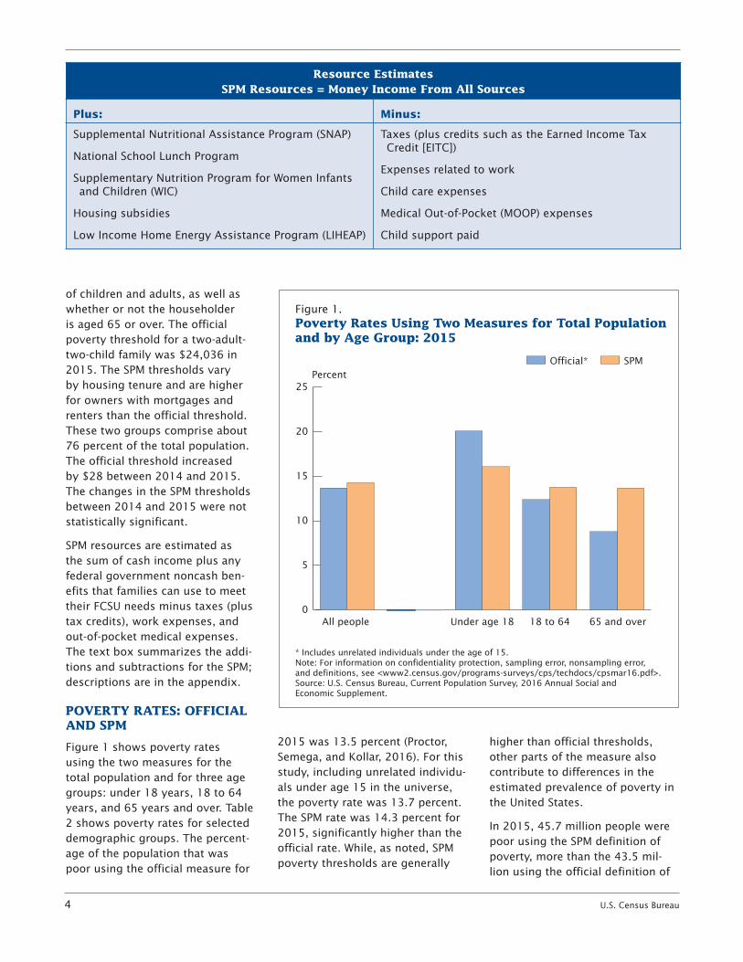
Figure 1 shows poverty rates using the two measures for the total population and for three age groups: under 18 years, 18 to 64 years, and 65 years and over. Table 2 shows poverty rates for selected demographic groups. The percent-age of the population that was poor using the official measure for

2015 was 13.5 percent (Proctor, Semega, and Kollar, 2016). For this study, including unrelated individu-als under age 15 in the universe, the poverty rate was 13.7 percent. The SPM rate was 14.3 percent for 2015, significantly higher than the official rate. While, as noted, SPM poverty thresholds are generally

higher than official thresholds, other parts of the measure also contribute to differences in the estimated prevalence of poverty in the United States.

In 2015, 45.7 million people were poor using the SPM definition of poverty, more than the 43.5 mil-lion using the official definition of

Figure 1.Poverty Rates Using Two Measures for Total Population and by Age Group: 2015

* Includes unrelated individuals under the age of 15.Note: For information on confidentiality protection, sampling error, nonsampling error, and definitions, see <www2.census.gov/programs-surveys/cps/techdocs/cpsmar16.pdf>.Source: U.S. Census Bureau, Current Population Survey, 2016 Annual Social and Economic Supplement.

0

5

10

15

20

25Percent

Official* SPM

All people Under age 18 18 to 64 65 and over

Resource EstimatesSPM Resources = Money Income From All Sources

Plus: Minus:

Supplemental Nutritional Assistance Program (SNAP)

National School Lunch Program

Supplementary Nutrition Program for Women Infants and Children (WIC)

Housing subsidies

Low Income Home Energy Assistance Program (LIHEAP)

Taxes (plus credits such as the Earned Income Tax Credit [EITC])

Expenses related to work

Child care expenses

Medical Out-of-Pocket (MOOP) expenses

Child support paid


Table 2.Number and Percentage of People in Poverty by Different Poverty Measures: 2015—Con.(Numbers in thousands, margin of error in thousands or percentage points as appropriate. For information on confidentiality pro-tection, sampling error, nonsampling error, and definitions, see www2.census.gov/programs-surveys/cps/techdocs/cpsmar16.pdf)

CharacteristicNumber**

(in thousands)

Official** SPMDifference

Number Percent Number Percent

Esti-mate

Margin of

error† (±)

Esti-mate

Margin of

error† (±)

Esti-mate

Margin of

error† (±)

Esti-mate

Margin of

error† (±) Number Percent

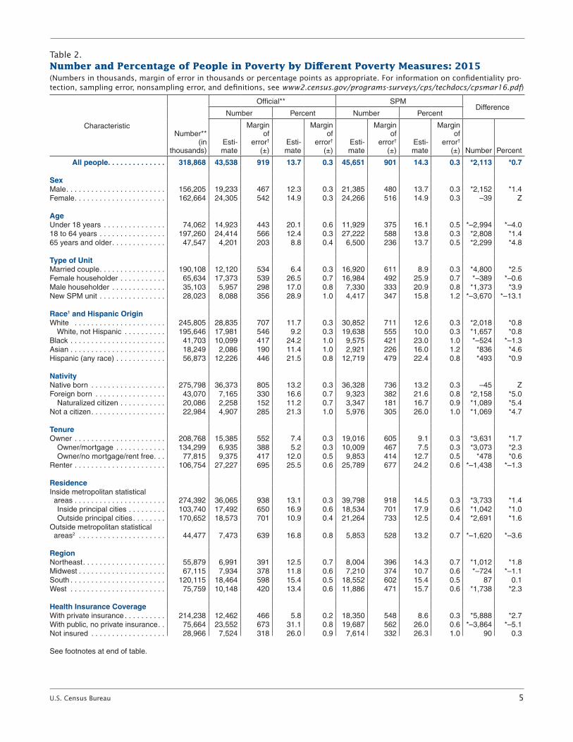
All people . . . . . . . . . . . . . . 318,868 43,538 919 13 .7 0 .3 45,651 901 14 .3 0 .3 *2,113 *0 .7

SexMale . . . . . . . . . . . . . . . . . . . . . . . . 156,205 19,233 467 12 .3 0 .3 21,385 480 13 .7 0 .3 *2,152 *1 .4Female . . . . . . . . . . . . . . . . . . . . . . 162,664 24,305 542 14 .9 0 .3 24,266 516 14 .9 0 .3 –39 Z

AgeUnder 18 years . . . . . . . . . . . . . . . 74,062 14,923 443 20 .1 0 .6 11,929 375 16 .1 0 .5 *–2,994 *–4 .018 to 64 years . . . . . . . . . . . . . . . . 197,260 24,414 566 12 .4 0 .3 27,222 588 13 .8 0 .3 *2,808 *1 .465 years and older . . . . . . . . . . . . . 47,547 4,201 203 8 .8 0 .4 6,500 236 13 .7 0 .5 *2,299 *4 .8

Type of UnitMarried couple . . . . . . . . . . . . . . . . 190,108 12,120 534 6 .4 0 .3 16,920 611 8 .9 0 .3 *4,800 *2 .5Female householder . . . . . . . . . . . 65,634 17,373 539 26 .5 0 .7 16,984 492 25 .9 0 .7 *–389 *–0 .6Male householder . . . . . . . . . . . . . 35,103 5,957 298 17 .0 0 .8 7,330 333 20 .9 0 .8 *1,373 *3 .9New SPM unit . . . . . . . . . . . . . . . . 28,023 8,088 356 28 .9 1 .0 4,417 347 15 .8 1 .2 *–3,670 *–13 .1

Race1 and Hispanic OriginWhite . . . . . . . . . . . . . . . . . . . . . . 245,805 28,835 707 11 .7 0 .3 30,852 711 12 .6 0 .3 *2,018 *0 .8 White, not Hispanic . . . . . . . . . . 195,646 17,981 546 9 .2 0 .3 19,638 555 10 .0 0 .3 *1,657 *0 .8Black . . . . . . . . . . . . . . . . . . . . . . . 41,703 10,099 417 24 .2 1 .0 9,575 421 23 .0 1 .0 *–524 *–1 .3Asian . . . . . . . . . . . . . . . . . . . . . . . 18,249 2,086 190 11 .4 1 .0 2,921 226 16 .0 1 .2 *836 *4 .6Hispanic (any race) . . . . . . . . . . . . 56,873 12,226 446 21 .5 0 .8 12,719 479 22 .4 0 .8 *493 *0 .9

NativityNative born . . . . . . . . . . . . . . . . . . 275,798 36,373 805 13 .2 0 .3 36,328 736 13 .2 0 .3 –45 ZForeign born . . . . . . . . . . . . . . . . . 43,070 7,165 330 16 .6 0 .7 9,323 382 21 .6 0 .8 *2,158 *5 .0 Naturalized citizen . . . . . . . . . . . 20,086 2,258 152 11 .2 0 .7 3,347 181 16 .7 0 .9 *1,089 *5 .4Not a citizen . . . . . . . . . . . . . . . . . . 22,984 4,907 285 21 .3 1 .0 5,976 305 26 .0 1 .0 *1,069 *4 .7

TenureOwner . . . . . . . . . . . . . . . . . . . . . . 208,768 15,385 552 7 .4 0 .3 19,016 605 9 .1 0 .3 *3,631 *1 .7 Owner/mortgage . . . . . . . . . . . . 134,299 6,935 388 5 .2 0 .3 10,009 467 7 .5 0 .3 *3,073 *2 .3 Owner/no mortgage/rent free . . . 77,815 9,375 417 12 .0 0 .5 9,853 414 12 .7 0 .5 *478 *0 .6Renter . . . . . . . . . . . . . . . . . . . . . . 106,754 27,227 695 25 .5 0 .6 25,789 677 24 .2 0 .6 *–1,438 *–1 .3

ResidenceInside metropolitan statistical areas . . . . . . . . . . . . . . . . . . . . . . 274,392 36,065 938 13 .1 0 .3 39,798 918 14 .5 0 .3 *3,733 *1 .4 Inside principal cities . . . . . . . . . 103,740 17,492 650 16 .9 0 .6 18,534 701 17 .9 0 .6 *1,042 *1 .0 Outside principal cities . . . . . . . . 170,652 18,573 701 10 .9 0 .4 21,264 733 12 .5 0 .4 *2,691 *1 .6Outside metropolitan statistical areas2 . . . . . . . . . . . . . . . . . . . . . 44,477 7,473 639 16 .8 0 .8 5,853 528 13 .2 0 .7 *–1,620 *–3 .6

RegionNortheast . . . . . . . . . . . . . . . . . . . . 55,879 6,991 391 12 .5 0 .7 8,004 396 14 .3 0 .7 *1,012 *1 .8Midwest . . . . . . . . . . . . . . . . . . . . . 67,115 7,934 378 11 .8 0 .6 7,210 374 10 .7 0 .6 *–724 *–1 .1South . . . . . . . . . . . . . . . . . . . . . . . 120,115 18,464 598 15 .4 0 .5 18,552 602 15 .4 0 .5 87 0 .1West . . . . . . . . . . . . . . . . . . . . . . . 75,759 10,148 420 13 .4 0 .6 11,886 471 15 .7 0 .6 *1,738 *2 .3

Health Insurance CoverageWith private insurance . . . . . . . . . . 214,238 12,462 466 5 .8 0 .2 18,350 548 8 .6 0 .3 *5,888 *2 .7With public, no private insurance . . 75,664 23,552 673 31 .1 0 .8 19,687 562 26 .0 0 .6 *–3,864 *–5 .1Not insured . . . . . . . . . . . . . . . . . . 28,966 7,524 318 26 .0 0 .9 7,614 332 26 .3 1 .0 90 0 .3

See footnotes at end of table .


poverty with the adjusted universe. While for most groups, SPM rates were higher than official poverty rates, the SPM shows lower pov-erty rates for children, individuals living in female householder units, individuals included in new SPM Resource Units, Blacks, renters, those living outside metropolitan areas, residents of the Midwest, those covered by only public health insurance, and individuals with a disability. Most other groups had higher poverty rates using the SPM, rather than the official measure. Official and SPM poverty rates for females, individuals born in the United States, residents of the South, the uninsured, and indi-viduals who did not work were not statistically different. Note that poverty rates for those 65 years

and over were higher under the SPM compared with the official measure. This partially reflects that the official thresholds are set lower for individuals with householders in this age group, while the SPM thresholds do not vary by age.11

Distribution of Income-to-Poverty Threshold Ratios: Official and SPM

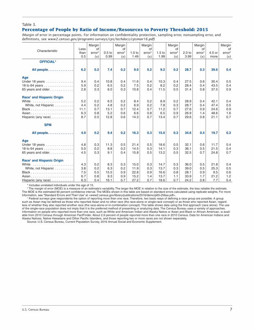
Comparing the distribution of gross cash income with that of SPM resources also allows an examina-tion of the effect of taxes and non-cash transfers on SPM rates. Table 3 shows the distribution of income-to-poverty threshold ratios for various groups. Dividing income by the respective poverty threshold

11 For more information about the SPM and those 65 years and older, see Bridges and Gesumaria (2013).

controls income by unit size and composition. Figure 2 shows the percent distribution of income-to-threshold ratio categories for all people, individuals under 18 years old and individuals 65 years old and over.

In general, the comparison sug-gests that a smaller percentage of the population was in the lowest category of the distribution using the SPM. For most groups, including targeted noncash benefits reduced the percentage of the population in the lowest category—those with income below half their poverty threshold. This was true for the age groups shown in Table 3, except for those over age 64. They showed a higher percentage below half of the poverty line with the SPM—4.5 percent compared to 2.8 percent

Table 2.Number and Percentage of People in Poverty by Different Poverty Measures: 2015—Con.(Numbers in thousands, margin of error in thousands or percentage points as appropriate. For information on confidentiality pro-tection, sampling error, nonsampling error, and definitions, see www2.census.gov/programs-surveys/cps/techdocs/cpsmar16.pdf)

CharacteristicNumber**

(in thousands)



Esti-mate

Margin of

error† (±)

Esti-mate

Margin of

error† (±)

Esti-mate

Margin of

error† (±)

Esti-mate

Margin of

error† (±) Number Percent

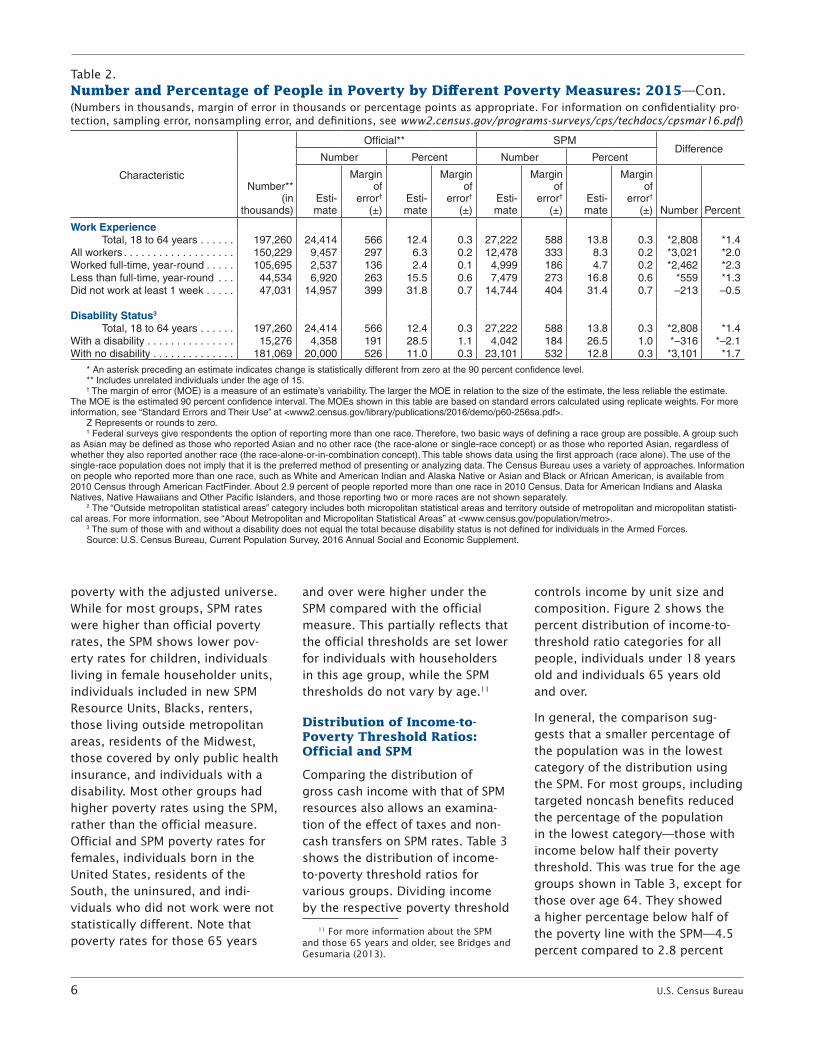
Work Experience Total, 18 to 64 years . . . . . . 197,260 24,414 566 12 .4 0 .3 27,222 588 13 .8 0 .3 *2,808 *1 .4All workers . . . . . . . . . . . . . . . . . . . 150,229 9,457 297 6 .3 0 .2 12,478 333 8 .3 0 .2 *3,021 *2 .0Worked full-time, year-round . . . . . 105,695 2,537 136 2 .4 0 .1 4,999 186 4 .7 0 .2 *2,462 *2 .3Less than full-time, year-round . . . 44,534 6,920 263 15 .5 0 .6 7,479 273 16 .8 0 .6 *559 *1 .3Did not work at least 1 week . . . . . 47,031 14,957 399 31 .8 0 .7 14,744 404 31 .4 0 .7 –213 –0 .5

Disability Status3

Total, 18 to 64 years . . . . . . 197,260 24,414 566 12 .4 0 .3 27,222 588 13 .8 0 .3 *2,808 *1 .4With a disability . . . . . . . . . . . . . . . 15,276 4,358 191 28 .5 1 .1 4,042 184 26 .5 1 .0 *–316 *–2 .1With no disability . . . . . . . . . . . . . . 181,069 20,000 526 11 .0 0 .3 23,101 532 12 .8 0 .3 *3,101 *1 .7

* An asterisk preceding an estimate indicates change is statistically different from zero at the 90 percent confidence level .** Includes unrelated individuals under the age of 15 .† The margin of error (MOE) is a measure of an estimate’s variability . The larger the MOE in relation to the size of the estimate, the less reliable the estimate .

The MOE is the estimated 90 percent confidence interval . The MOEs shown in this table are based on standard errors calculated using replicate weights . For more information, see “Standard Errors and Their Use” at <www2 .census .gov/library/publications/2016/demo/p60-256sa .pdf> .

Z Represents or rounds to zero .1 Federal surveys give respondents the option of reporting more than one race . Therefore, two basic ways of defining a race group are possible . A group such

as Asian may be defined as those who reported Asian and no other race (the race-alone or single-race concept) or as those who reported Asian, regardless of whether they also reported another race (the race-alone-or-in-combination concept) . This table shows data using the first approach (race alone) . The use of the single-race population does not imply that it is the preferred method of presenting or analyzing data . The Census Bureau uses a variety of approaches . Information on people who reported more than one race, such as White and American Indian and Alaska Native or Asian and Black or African American, is available from 2010 Census through American FactFinder . About 2 .9 percent of people reported more than one race in 2010 Census . Data for American Indians and Alaska Natives, Native Hawaiians and Other Pacific Islanders, and those reporting two or more races are not shown separately .

2 The “Outside metropolitan statistical areas” category includes both micropolitan statistical areas and territory outside of metropolitan and micropolitan statisti-cal areas . For more information, see “About Metropolitan and Micropolitan Statistical Areas” at <www .census .gov/population/metro> .

3 The sum of those with and without a disability does not equal the total because disability status is not defined for individuals in the Armed Forces .Source: U .S . Census Bureau, Current Population Survey, 2016 Annual Social and Economic Supplement .


Table 3.Percentage of People by Ratio of Income/Resources to Poverty Threshold: 2015(Margin of error in percentage points. For information on confidentiality protection, sampling error, nonsampling error, and definitions, see www2.census.gov/programs-surveys/cps/techdocs/cpsmar16.pdf)

Characteristic Less than 0 .5

Margin of

error† (±)

0 .5 to 0 .99

Margin of

error† (±)

1 .0 to 1 .49

Margin of

error† (±)

1 .5 to 1 .99

Margin of

error† (±)

2 .0 to 3 .99

Margin of

error† (±)

4 .0 or more

Margin of

error† (±)

OFFICIAL*

All people . . . . . . . . . . . . . . 6 .2 0 .2 7 .4 0 .2 9 .0 0 .2 9 .2 0 .2 28 .7 0 .3 39 .6 0 .4

AgeUnder 18 years . . . . . . . . . . . . . . . 9 .4 0 .4 10 .8 0 .4 11 .6 0 .4 10 .3 0 .4 27 .5 0 .6 30 .4 0 .518 to 64 years . . . . . . . . . . . . . . . . 5 .9 0 .2 6 .5 0 .2 7 .5 0 .2 8 .2 0 .2 28 .4 0 .4 43 .5 0 .465 years and older . . . . . . . . . . . . . 2 .8 0 .3 6 .0 0 .3 10 .8 0 .4 11 .5 0 .5 31 .4 0 .8 37 .5 0 .9

Race1 and Hispanic OriginWhite . . . . . . . . . . . . . . . . . . . . . . 5 .2 0 .2 6 .5 0 .2 8 .4 0 .2 8 .9 0 .2 28 .9 0 .4 42 .1 0 .4 White, not Hispanic . . . . . . . . . . 4 .4 0 .2 4 .8 0 .2 6 .9 0 .2 7 .8 0 .3 28 .7 0 .4 47 .4 0 .5Black . . . . . . . . . . . . . . . . . . . . . . . 11 .1 0 .7 13 .1 0 .7 12 .4 0 .7 11 .2 0 .7 27 .6 0 .9 24 .6 0 .9Asian . . . . . . . . . . . . . . . . . . . . . . . 6 .3 0 .8 5 .2 0 .6 6 .6 0 .8 6 .5 0 .9 26 .9 1 .4 48 .6 1 .6Hispanic (any race) . . . . . . . . . . . . 8 .7 0 .5 12 .8 0 .6 14 .3 0 .7 13 .4 0 .7 29 .6 0 .8 21 .1 0 .7

SPM

All people . . . . . . . . . . . . . . 4 .9 0 .2 9 .4 0 .2 16 .3 0 .3 15 .0 0 .3 34 .6 0 .4 19 .7 0 .3

AgeUnder 18 years . . . . . . . . . . . . . . . 4 .8 0 .3 11 .3 0 .5 21 .4 0 .5 18 .6 0 .5 32 .1 0 .6 11 .7 0 .418 to 64 years . . . . . . . . . . . . . . . . 5 .0 0 .2 8 .8 0 .2 14 .5 0 .3 14 .1 0 .3 36 .1 0 .5 21 .5 0 .465 years and older . . . . . . . . . . . . . 4 .5 0 .3 9 .1 0 .4 15 .8 0 .5 13 .2 0 .5 32 .5 0 .7 24 .8 0 .7

Race1 and Hispanic OriginWhite . . . . . . . . . . . . . . . . . . . . . . 4 .3 0 .2 8 .3 0 .3 15 .0 0 .3 14 .7 0 .3 36 .0 0 .5 21 .8 0 .4 White, not Hispanic . . . . . . . . . . 3 .8 0 .2 6 .3 0 .2 11 .9 0 .3 13 .7 0 .3 39 .0 0 .5 25 .3 0 .5Black . . . . . . . . . . . . . . . . . . . . . . . 7 .5 0 .5 15 .5 0 .9 22 .8 0 .9 16 .6 0 .8 28 .1 0 .9 9 .5 0 .6Asian . . . . . . . . . . . . . . . . . . . . . . . 6 .7 0 .8 9 .3 0 .9 15 .2 1 .4 13 .7 1 .1 33 .9 1 .7 21 .2 1 .2Hispanic (any race) . . . . . . . . . . . . 6 .3 0 .4 16 .1 0 .7 27 .2 0 .7 18 .6 0 .7 24 .2 0 .8 7 .7 0 .4

* Includes unrelated individuals under the age of 15 .† The margin of error (MOE) is a measure of an estimate’s variability . The larger the MOE in relation to the size of the estimate, the less reliable the estimate .


1 Federal surveys give respondents the option of reporting more than one race . Therefore, two basic ways of defining a race group are possible . A group such as Asian may be defined as those who reported Asian and no other race (the race-alone or single-race concept) or as those who reported Asian, regard-less of whether they also reported another race (the race-alone-or-in-combination concept) . This table shows data using the first approach (race alone) . The use of the single-race population does not imply that it is the preferred method of presenting or analyzing data . The Census Bureau uses a variety of approaches . Information on people who reported more than one race, such as White and American Indian and Alaska Native or Asian and Black or African American, is avail-able from 2010 Census through American FactFinder . About 2 .9 percent of people reported more than one race in 2010 Census . Data for American Indians and Alaska Natives, Native Hawaiians and Other Pacific Islanders, and those reporting two or more races are not shown separately .

Source: U .S . Census Bureau, Current Population Survey, 2016 Annual Social and Economic Supplement .


with the official measure. Many of the noncash benefits included in the SPM are not targeted to this population. Further, many transfers received by this group are in cash, especially Social Security payments, and are captured in the official mea-sure, as well as the SPM. Note that the percentage of the 65 years and over age group with cash income below half their threshold was lower than that of other age groups using the official measure (2.8 percent), while the percentage for children was higher (9.4 percent). Subtracting Medical Out-of-Pocket (MOOP) and other expenses and adding noncash benefits in the SPM

narrowed the differences across the three age groups.12

On the other hand, the SPM shows a smaller percentage with income or resources in the high-est category—four or more times the thresholds. The SPM resource measure subtracts taxes—com-pared with the official measure, which does not—bringing down the percentage of people with income in the highest category.

12 The differences in the percentage of children with SPM resources under half their threshold and the percentage of individuals in the other age groups under half their thresh-old were not statistically significant. There was a lower percentage of individuals aged 65 and over below half their threshold than the percentage of individuals 18 to 64 years of age in this range.

Another notable difference between the distributions using these two measures was the larger num-ber of individuals with income-to-threshold ratios in the middle categories, between 1.0 and 3.99, with the SPM. Since the effect of taxes and transfers is often to move family income from the extremes of the distribution to the center of the distribution, that is, from the very bottom with targeted transfers or from the very top via taxes and other expenses, the increase in the size of these middle categories is to be expected.

Table 3 shows similar calcula-tions by race and ethnicity. Using the SPM, smaller percentages had

Figure 2.Distribution of People by Income-to-Threshold Ratios: 2015(In percent)



Total population

6.2

4.5

9.4 10.8

4.8

2.8

4.5

Under 18 years

65 years and over

Less than 0.5 0.5 to 0.99 1.0 to 1.99 2.0 to 3.99 4.0 or more

SPM

Official*

SPM

Official*

SPM

Official* 7.4

9.4

11.3

6.0

9.1 29.0

15.7

40.0

21.9

31.3

14.2 28.7

34.6

27.5

32.1

31.4

32.5 24.8

37.5

11.7

30.4

19.7

39.6


Table 4.Number and Percentage of People in Poverty by State Using 3-Year Average Over 2013, 2014, and 2015—Con.(Numbers in thousands, margin of error in thousands or percentage points as appropriate. Data for 2013 are based on the CPS ASEC sample of 30,000 addresses.1 For information on confidentiality protection, sampling error, nonsampling error, and defini-tions, see www2.census.gov/programs-surveys/cps/techdocs/cpsmar16.pdf)

Characteristic



EstimateMargin of error† (±) Estimate

Margin of error† (±) Estimate


Margin of error† (±) Number Percent

United States . . . . . . . . . . . . . . . . . . 45,725 703 14 .5 0 .2 47,823 686 15 .1 0 .2 *2,098 *0 .7

Alabama . . . . . . . . . . . . . . . . . . . . . . 847 60 17 .6 1 .3 665 63 13 .8 1 .3 *–182 *–3 .8Alaska . . . . . . . . . . . . . . . . . . . . . . . . 73 10 10 .4 1 .4 81 11 11 .7 1 .6 *9 *1 .3Arizona . . . . . . . . . . . . . . . . . . . . . . . 1,246 94 18 .8 1 .4 1,163 84 17 .5 1 .3 –83 –1 .3Arkansas . . . . . . . . . . . . . . . . . . . . . . 472 39 16 .3 1 .4 418 47 14 .4 1 .7 *–54 *–1 .9California . . . . . . . . . . . . . . . . . . . . . . 5,803 285 15 .0 0 .7 7,959 298 20 .6 0 .8 *2,157 *5 .6

Colorado . . . . . . . . . . . . . . . . . . . . . . 591 69 11 .0 1 .3 601 63 11 .2 1 .2 10 0 .2Connecticut . . . . . . . . . . . . . . . . . . . . 344 49 9 .6 1 .4 460 51 12 .8 1 .4 *116 *3 .2Delaware . . . . . . . . . . . . . . . . . . . . . . 105 13 11 .2 1 .4 113 15 12 .1 1 .6 8 0 .9District of Columbia . . . . . . . . . . . . . . 130 11 19 .6 1 .7 147 13 22 .2 2 .0 *17 *2 .6Florida . . . . . . . . . . . . . . . . . . . . . . . . 3,172 187 16 .0 1 .0 3,766 221 19 .0 1 .1 *594 *3 .0

Georgia . . . . . . . . . . . . . . . . . . . . . . . 1,788 131 17 .9 1 .3 1,678 127 16 .8 1 .3 –109 –1 .1Hawaii . . . . . . . . . . . . . . . . . . . . . . . . 149 19 10 .9 1 .4 229 23 16 .8 1 .7 *81 *5 .9Idaho . . . . . . . . . . . . . . . . . . . . . . . . . 204 25 12 .5 1 .6 176 25 10 .8 1 .6 *–28 *–1 .7Illinois . . . . . . . . . . . . . . . . . . . . . . . . . 1,636 121 12 .9 0 .9 1,747 135 13 .7 1 .1 *111 *0 .9Indiana . . . . . . . . . . . . . . . . . . . . . . . . 978 111 15 .0 1 .7 806 88 12 .4 1 .4 *–171 *–2 .6

Iowa . . . . . . . . . . . . . . . . . . . . . . . . . . 351 38 11 .4 1 .3 325 40 10 .5 1 .3 –26 –0 .8Kansas . . . . . . . . . . . . . . . . . . . . . . . . 356 48 12 .6 1 .7 281 38 9 .9 1 .3 *–76 *–2 .7Kentucky . . . . . . . . . . . . . . . . . . . . . . 913 73 20 .7 1 .7 706 78 16 .0 1 .8 *–207 *–4 .7Louisiana . . . . . . . . . . . . . . . . . . . . . . 961 82 21 .0 1 .8 816 64 17 .9 1 .4 *–145 *–3 .2Maine . . . . . . . . . . . . . . . . . . . . . . . . . 171 21 12 .9 1 .6 135 17 10 .2 1 .2 *–36 *–2 .7

Maryland . . . . . . . . . . . . . . . . . . . . . . 599 79 10 .1 1 .3 847 81 14 .3 1 .4 *249 *4 .2Massachusetts . . . . . . . . . . . . . . . . . . 839 108 12 .5 1 .6 1,013 115 15 .1 1 .7 *174 *2 .6Michigan . . . . . . . . . . . . . . . . . . . . . . 1,340 118 13 .5 1 .2 1,189 107 12 .0 1 .1 *–151 *–1 .5Minnesota . . . . . . . . . . . . . . . . . . . . . 492 66 9 .1 1 .2 492 63 9 .1 1 .2 Z ZMississippi . . . . . . . . . . . . . . . . . . . . . 593 61 20 .2 2 .0 498 54 17 .0 1 .9 *–95 *–3 .2

Missouri . . . . . . . . . . . . . . . . . . . . . . . 757 98 12 .7 1 .6 692 77 11 .6 1 .3 –65 –1 .1Montana . . . . . . . . . . . . . . . . . . . . . . . 116 19 11 .5 1 .9 99 16 9 .8 1 .5 *–17 *–1 .7Nebraska . . . . . . . . . . . . . . . . . . . . . . 207 25 11 .0 1 .3 171 24 9 .1 1 .3 *–36 *–1 .9Nevada . . . . . . . . . . . . . . . . . . . . . . . 422 49 14 .9 1 .8 479 50 17 .0 1 .8 *57 *2 .0New Hampshire . . . . . . . . . . . . . . . . . 87 12 6 .7 0 .9 113 15 8 .7 1 .1 *26 *2 .0

New Jersey . . . . . . . . . . . . . . . . . . . . 962 109 10 .8 1 .2 1,342 122 15 .1 1 .4 *380 *4 .3New Mexico . . . . . . . . . . . . . . . . . . . . 451 51 22 .0 2 .5 352 42 17 .1 2 .0 *–99 *–4 .8New York . . . . . . . . . . . . . . . . . . . . . . 3,010 195 15 .4 1 .0 3,502 216 17 .9 1 .1 *492 *2 .5North Carolina . . . . . . . . . . . . . . . . . . 1,547 139 15 .8 1 .4 1,365 116 13 .9 1 .2 *–182 *–1 .9North Dakota . . . . . . . . . . . . . . . . . . . 84 11 11 .4 1 .5 76 10 10 .3 1 .3 –8 –1 .1

Ohio . . . . . . . . . . . . . . . . . . . . . . . . . . 1,697 133 14 .8 1 .2 1,392 129 12 .2 1 .1 *–305 *–2 .7Oklahoma . . . . . . . . . . . . . . . . . . . . . 671 80 17 .8 2 .2 523 53 13 .8 1 .4 *–149 *–3 .9Oregon . . . . . . . . . . . . . . . . . . . . . . . . 542 67 13 .6 1 .6 535 66 13 .4 1 .6 –7 –0 .2Pennsylvania . . . . . . . . . . . . . . . . . . . 1,535 132 12 .1 1 .0 1,594 135 12 .6 1 .1 59 0 .5Rhode Island . . . . . . . . . . . . . . . . . . . 115 17 11 .0 1 .6 122 19 11 .7 1 .8 7 0 .7

South Carolina . . . . . . . . . . . . . . . . . . 793 80 16 .7 1 .7 773 71 16 .3 1 .5 –20 –0 .4South Dakota . . . . . . . . . . . . . . . . . . . 113 17 13 .4 2 .1 86 12 10 .2 1 .5 *–26 *–3 .2Tennessee . . . . . . . . . . . . . . . . . . . . . 1,030 92 15 .9 1 .4 1,003 108 15 .5 1 .7 –27 –0 .4Texas . . . . . . . . . . . . . . . . . . . . . . . . . 4,299 234 16 .1 0 .9 4,001 222 14 .9 0 .8 *–298 *–1 .1Utah . . . . . . . . . . . . . . . . . . . . . . . . . . 312 42 10 .6 1 .4 301 40 10 .2 1 .4 –11 –0 .4



income below half of their poverty thresholds, compared with the official measure for the race and ethnicity groups shown, except for Asians. For Blacks, the percentage in this lowest category was 11.1 percent with the official measure and 7.5 percent with the SPM. Percentages of Whites and Hispan-ics in the lowest category were also lower using the SPM.

Poverty Rates by State: Official and SPM

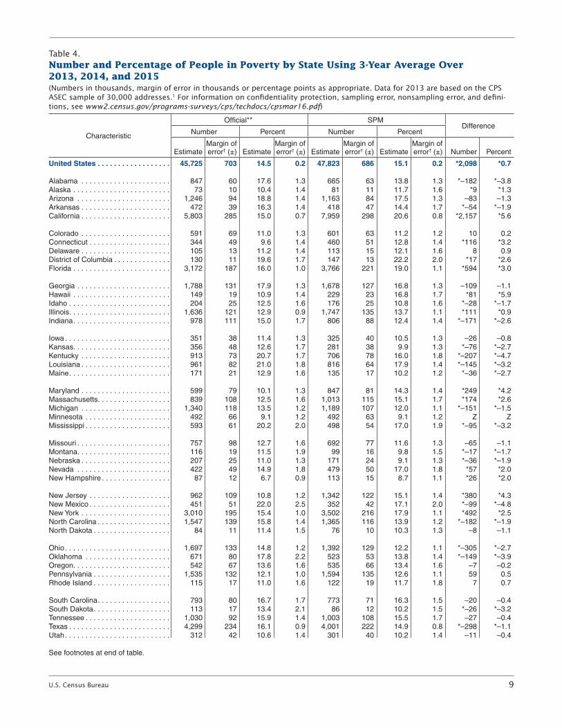
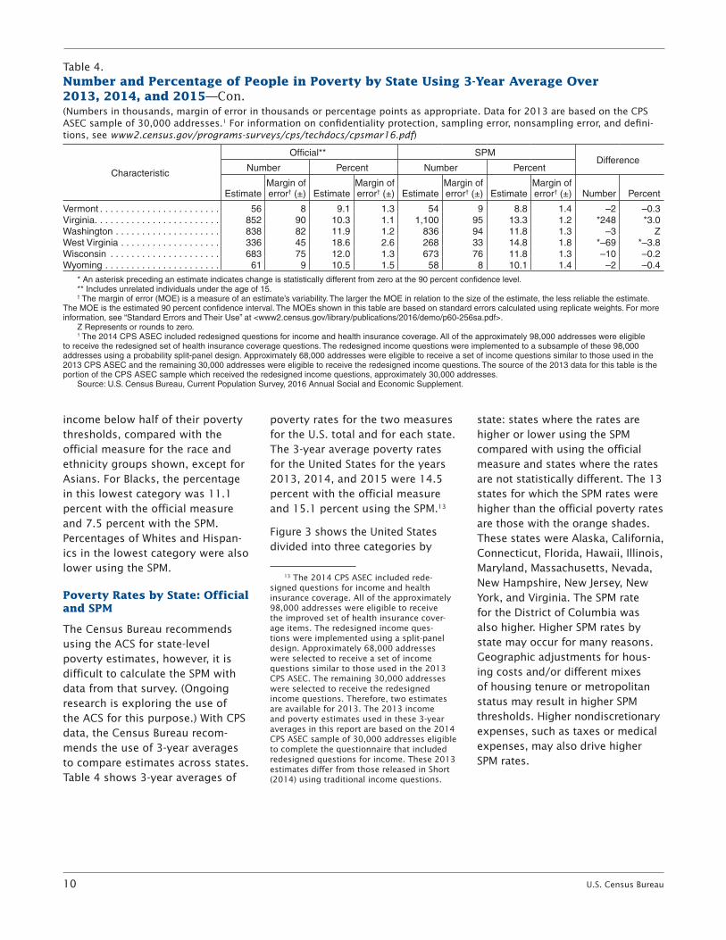
The Census Bureau recommends using the ACS for state-level poverty estimates, however, it is difficult to calculate the SPM with data from that survey. (Ongoing research is exploring the use of the ACS for this purpose.) With CPS data, the Census Bureau recom-mends the use of 3-year averages to compare estimates across states. Table 4 shows 3-year averages of

poverty rates for the two measures for the U.S. total and for each state. The 3-year average poverty rates for the United States for the years 2013, 2014, and 2015 were 14.5 percent with the official measure and 15.1 percent using the SPM.13

Figure 3 shows the United States divided into three categories by

13 The 2014 CPS ASEC included rede-signed questions for income and health insurance coverage. All of the approximately 98,000 addresses were eligible to receive the improved set of health insurance cover-age items. The redesigned income ques-tions were implemented using a split-panel design. Approximately 68,000 addresses were selected to receive a set of income questions similar to those used in the 2013 CPS ASEC. The remaining 30,000 addresses were selected to receive the redesigned income questions. Therefore, two estimates are available for 2013. The 2013 income and poverty estimates used in these 3-year averages in this report are based on the 2014 CPS ASEC sample of 30,000 addresses eligible to complete the questionnaire that included redesigned questions for income. These 2013 estimates differ from those released in Short (2014) using traditional income questions.

state: states where the rates are higher or lower using the SPM compared with using the official measure and states where the rates are not statistically different. The 13 states for which the SPM rates were higher than the official poverty rates are those with the orange shades. These states were Alaska, California, Connecticut, Florida, Hawaii, Illinois, Maryland, Massachusetts, Nevada, New Hampshire, New Jersey, New York, and Virginia. The SPM rate for the District of Columbia was also higher. Higher SPM rates by state may occur for many reasons. Geographic adjustments for hous-ing costs and/or different mixes of housing tenure or metropolitan status may result in higher SPM thresholds. Higher nondiscretionary expenses, such as taxes or medical expenses, may also drive higher SPM rates.

Table 4.Number and Percentage of People in Poverty by State Using 3-Year Average Over 2013, 2014, and 2015—Con.(Numbers in thousands, margin of error in thousands or percentage points as appropriate. Data for 2013 are based on the CPS ASEC sample of 30,000 addresses.1 For information on confidentiality protection, sampling error, nonsampling error, and defini-tions, see www2.census.gov/programs-surveys/cps/techdocs/cpsmar16.pdf)

Characteristic






Margin of error† (±) Number Percent

Vermont . . . . . . . . . . . . . . . . . . . . . . . 56 8 9 .1 1 .3 54 9 8 .8 1 .4 –2 –0 .3Virginia . . . . . . . . . . . . . . . . . . . . . . . . 852 90 10 .3 1 .1 1,100 95 13 .3 1 .2 *248 *3 .0Washington . . . . . . . . . . . . . . . . . . . . 838 82 11 .9 1 .2 836 94 11 .8 1 .3 –3 ZWest Virginia . . . . . . . . . . . . . . . . . . . 336 45 18 .6 2 .6 268 33 14 .8 1 .8 *–69 *–3 .8Wisconsin . . . . . . . . . . . . . . . . . . . . . 683 75 12 .0 1 .3 673 76 11 .8 1 .3 –10 –0 .2Wyoming . . . . . . . . . . . . . . . . . . . . . . 61 9 10 .5 1 .5 58 8 10 .1 1 .4 –2 –0 .4

* An asterisk preceding an estimate indicates change is statistically different from zero at the 90 percent confidence level .** Includes unrelated individuals under the age of 15 .† The margin of error (MOE) is a measure of an estimate’s variability . The larger the MOE in relation to the size of the estimate, the less reliable the estimate .


Z Represents or rounds to zero .1 The 2014 CPS ASEC included redesigned questions for income and health insurance coverage . All of the approximately 98,000 addresses were eligible

to receive the redesigned set of health insurance coverage questions . The redesigned income questions were implemented to a subsample of these 98,000 addresses using a probability split-panel design . Approximately 68,000 addresses were eligible to receive a set of income questions similar to those used in the 2013 CPS ASEC and the remaining 30,000 addresses were eligible to receive the redesigned income questions . The source of the 2013 data for this table is the portion of the CPS ASEC sample which received the redesigned income questions, approximately 30,000 addresses .

Source: U .S . Census Bureau, Current Population Survey, 2016 Annual Social and Economic Supplement .


!!

!!

!!

!!

!!

!!

!

!!

!!

!!

!!

!!

!!

!!

!! DC

TX

CA

MT

AZ

ID

NV

NM

COIL

OR

UT

KS

WY

IANE

SD

MN

FL

ND

OK

WI

MO

WA

AL GA

LA

AR

MI

IN

PA

NY

NC

MS

TN

VAKY

OH

SC

ME

WV

VTNH

NJ

MACT

MDDE

RI

AK

HISource: U.S. Census Bureau, CurrentPopulation Survey, 2013 to 2015 AnnualSocial and Economic Supplements.

Not statistically different

SPM lower than official

Figure 3.

SPM higher than official

0 500 Miles

0 100 Miles

0 100 Miles

Figure 3.Difference in Poverty Rates by State Using the Official Measureand the SPM: 3-Year Average 2013 to 2015

Blue shades represent the 19 states where SPM rates were lower than the official poverty rates. These states were Alabama, Arkansas, Idaho, Indiana, Kansas, Kentucky, Louisiana, Maine, Michigan, Mississippi, Montana, Nebraska, New Mexico, North Carolina, Ohio, Oklahoma, South Dakota, Texas, and West Virginia. Lower SPM rates would occur due to lower thresh-olds reflecting lower housing costs, a different mix of housing tenure or metropolitan status, or more gener-ous noncash benefits. Gray shades are those 18 states that were not statistically different under the two measures and include Arizona, Colorado, Delaware, Georgia, Iowa, Minnesota, Missouri, North Dakota,

Oregon, Pennsylvania, Rhode Island, South Carolina, Tennessee, Utah, Vermont, Washington, Wisconsin, and Wyoming. Details are in Table 4.

The SPM and the Effect of Cash and Noncash Transfers, Taxes, and Other Nondiscretionary Expenses

This section moves away from comparing the SPM with the official measure and looks only at the SPM. This analysis allows one to gauge the effects of taxes and transfers and other necessary expenses using the SPM as the measure of economic well-being.

The official poverty measure takes account of cash benefits from the

government, such as Social Secu-rity and Unemployment Insurance benefits, Supplemental Security Income (SSI), public assistance ben-efits, such as Temporary Assistance for Needy Families (TANF), and workers’ compensation benefits, but does not take account of taxes or noncash benefits aimed at improving the economic situ-ation of the poor. Besides taking account of cash benefits and nec-essary expenses, such as MOOP expenses and expenses related to work, the SPM also accounts for taxes and noncash transfers. An important contribution of the SPM is that it allows us to gauge the potential magnitude of the effect of tax credits and transfers


Table 5a.Effect of Individual Elements on SPM Rates: 2015(Margin of error in percentage points. For information on confidentiality protection, sampling error, nonsampling error, and defini-tions, see www2.census.gov/programs-surveys/cps/techdocs/cpsmar16.pdf)

ElementAll people Under 18 years 18 to 64 years 65 years and over




Margin of error† (±)

All people . . . . . . . . . . . . . . . . . . . . . 14 .32 0 .28 16 .11 0 .50 13 .80 0 .30 13 .67 0 .50

ADDITIONSSocial Security . . . . . . . . . . . . . . . . . . . –8 .34 0 .19 –2 .12 0 .18 –3 .99 0 .16 –36 .04 0 .79Refundable tax credits . . . . . . . . . . . . . –2 .88 0 .13 –6 .52 0 .34 –2 .16 0 .10 –0 .19 0 .05SNAP . . . . . . . . . . . . . . . . . . . . . . . . . . –1 .44 0 .09 –2 .70 0 .21 –1 .13 0 .08 –0 .77 0 .11SSI . . . . . . . . . . . . . . . . . . . . . . . . . . . . –1 .04 0 .08 –0 .79 0 .12 –1 .07 0 .09 –1 .30 0 .16Housing subsidies . . . . . . . . . . . . . . . . –0 .80 0 .06 –1 .16 0 .14 –0 .61 0 .06 –0 .99 0 .14Child support received . . . . . . . . . . . . . –0 .43 0 .05 –1 .07 0 .13 –0 .29 0 .04 –0 .03 0 .02School lunch . . . . . . . . . . . . . . . . . . . . –0 .40 0 .05 –0 .96 0 .14 –0 .27 0 .03 –0 .03 0 .02TANF/general assistance . . . . . . . . . . . –0 .21 0 .04 –0 .47 0 .10 –0 .15 0 .03 –0 .02 0 .02Unemployment insurance . . . . . . . . . . –0 .20 0 .03 –0 .26 0 .06 –0 .23 0 .04 –0 .02 0 .01LIHEAP . . . . . . . . . . . . . . . . . . . . . . . . –0 .08 0 .02 –0 .10 0 .04 –0 .06 0 .02 –0 .10 0 .04Workers’ compensation . . . . . . . . . . . . –0 .12 0 .03 –0 .15 0 .07 –0 .13 0 .03 –0 .03 0 .02WIC . . . . . . . . . . . . . . . . . . . . . . . . . . . –0 .12 0 .04 –0 .29 0 .09 –0 .08 0 .02 Z Z

SUBTRACTIONSChild support paid . . . . . . . . . . . . . . . . 0 .08 0 .02 0 .07 0 .03 0 .10 0 .02 0 .02 0 .02Federal income tax . . . . . . . . . . . . . . . 0 .44 0 .05 0 .37 0 .07 0 .54 0 .06 0 .11 0 .05FICA . . . . . . . . . . . . . . . . . . . . . . . . . . 1 .52 0 .10 2 .07 0 .19 1 .58 0 .10 0 .41 0 .09Work expenses . . . . . . . . . . . . . . . . . . 1 .75 0 .10 2 .44 0 .22 1 .80 0 .10 0 .47 0 .09MOOP . . . . . . . . . . . . . . . . . . . . . . . . . 3 .52 0 .14 3 .41 0 .21 3 .05 0 .16 5 .65 0 .30

† The margin of error (MOE) is a measure of an estimate’s variability . The larger the MOE in relation to the size of the estimate, the less reliable the estimate . The MOE is the estimated 90 percent confidence interval . The MOEs shown in this table are based on standard errors calculated using replicate weights . For more information, see “Standard Errors and Their Use” at <www2 .census .gov/library/publications/2016/demo/p60-256sa .pdf> .

Z Represents or rounds to zero .Source: U .S . Census Bureau, Current Population Survey, 2016 Annual Social and Economic Supplement .

on alleviating poverty. We can also examine the effects of nondiscre-tionary expenses, such as work and MOOP expenses.

Table 5a shows the effect that vari-ous additions and subtractions had on the SPM rate in 2015, holding all else the same and assuming no behavioral changes. Additions and subtractions are shown for the total population and by three age groups. Additions shown in the table include cash benefits, also accounted for

in the official measure, as well as noncash benefits, included only in the SPM. This allows us to examine the effects of government transfers on poverty estimates. Since child support paid is subtracted from income, we also examine the effect of child support received on alleviat-ing poverty. Child support payments received are counted as income in both the official measure and the SPM. Table 5b shows the same set of additions and subtractions, but shows the number of people

affected by removing each ele-ment from the SPM, rather than the change in the SPM rate.

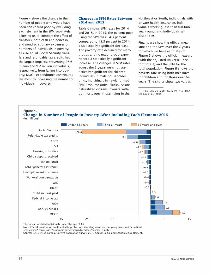
Removing one item from the calculation of SPM resources and recalculating poverty rates shows, for example, that without Social Security benefits the SPM rate would have been 8.3 percentage points higher (22.7 percent), rather than 14.3 percent. This means that, without Social Security benefits, an additional 26.6 million people


Table 5b.Effect of Individual Elements on the Number of Individuals in Poverty: 2015(Numbers and margin of error in thousands. For information on confidentiality protection, sampling error, nonsampling error, and definitions, see www2.census.gov/programs-surveys/cps/techdocs/cpsmar16.pdf)

ElementAll people Under 18 years 18 to 64 years 65 years and over




Margin of error† (±)

All people . . . . . . . . . . . . . . . . . . . 45,651 901 11,929 375 27,222 588 6,500 236

ADDITIONSSocial Security . . . . . . . . . . . . . . . . –26,585 600 –1,571 130 –7,878 315 –17,137 376Refundable tax credits . . . . . . . . . . –9,172 428 –4,829 249 –4,254 203 –89 23SNAP . . . . . . . . . . . . . . . . . . . . . . . –4,595 296 –2,001 153 –2,228 164 –366 54SSI . . . . . . . . . . . . . . . . . . . . . . . . . –3,313 248 –587 86 –2,107 169 –619 78Housing subsidies . . . . . . . . . . . . . –2,537 197 –861 104 –1,203 111 –473 67Child support received . . . . . . . . . . –1,383 162 –790 100 –577 76 –16 10School lunch . . . . . . . . . . . . . . . . . –1,262 167 –714 106 –534 68 –13 11TANF/general assistance . . . . . . . . –664 124 –351 77 –304 62 –9 9Unemployment insurance . . . . . . . –649 109 –191 48 –446 73 –12 7LIHEAP . . . . . . . . . . . . . . . . . . . . . –242 61 –71 33 –124 35 –46 21Workers’ compensation . . . . . . . . . –376 105 –114 52 –249 68 –14 11WIC . . . . . . . . . . . . . . . . . . . . . . . . –371 113 –215 69 –156 48 Z Z

SUBTRACTIONSChild support paid . . . . . . . . . . . . . 254 66 49 22 194 49 10 10Federal income tax . . . . . . . . . . . . 1,389 148 276 51 1,061 111 53 24FICA . . . . . . . . . . . . . . . . . . . . . . . 4,843 310 1,537 139 3,109 195 197 42Work expenses . . . . . . . . . . . . . . . 5,587 316 1,808 161 3,557 188 222 43MOOP . . . . . . . . . . . . . . . . . . . . . . 11,226 460 2,522 160 6,016 315 2,687 143

† The margin of error (MOE) is a measure of an estimate’s variability . The larger the MOE in relation to the size of the estimate, the less reliable the estimate . The MOE is the estimated 90 percent confidence interval . The MOEs shown in this table are based on standard errors calculated using replicate weights . For more information, see “Standard Errors and Their Use” at <www2 .census .gov/library/publications/2016/demo/p60-256sa .pdf> .

Z Represents or rounds to zero .Source: U .S . Census Bureau, Current Population Survey, 2016 Annual Social and Economic Supplement .

would be living below the pov-erty line, beyond the 45.7 million people classified as poor with the SPM. Not including refundable tax credits (the EITC and the refundable portion of the child tax credit) in resources, an additional 9.2 million people would have been considered poor, all else constant. On the other hand, removing amounts paid for child support, income and payroll taxes, work-related expenses, and MOOP expenses from the calcula-tion resulted in lower poverty rates.

Without subtracting MOOP expenses from income, the SPM rate would have been 3.5 percentage points lower. In numbers, 11.2 million fewer people would have been clas-sified as poor.

Tables 5a and 5b also show effects for different age groups. In 2015, not accounting for refundable tax credits would have resulted in a 6.5 percentage point increase in the child poverty rate, represent-ing 4.8 million children precluded

from poverty by the inclusion of these credits. Not subtracting MOOP expenses from the income of families with children would have resulted in a child poverty rate 3.4 percentage points lower. For the 65 years and over group, SPM rates increased by about 5.7 percentage points with the subtraction of MOOP expenses from income, while Social Security benefits lowered poverty rates by 36.0 percentage points, lift-ing 17.1 million individuals above the poverty line.


–35 –25 –15 –5 5 15

Figure 4.Change in Number of People in Poverty After Including Each Element: 2015(In millions)

* Includes unrelated individuals under the age of 15.Note: For information on confidentiality protection, sampling error, nonsampling error, and definitions, see: <www2.census.gov/programs-surveys/cps/techdocs/cpsmar16.pdf>.Source: U.S. Census Bureau, Current Population Survey, 2016 Annual Social and Economic Supplement.

Under 18 years 18 to 64 years 65 years and over

Social Security

Refundable tax credits

SNAP

SSI

Housing subsidies

Child support received

School lunch

TANF/general assistance

Unemployment insurance

Workers' compensation

WIC

LIHEAP

Child support paid

Federal income tax

FICA

Work expenses

MOOP

–26.6

–2.5

–1.4

–1.3

–0.7

–0.6

–0.4

–0.4

–0.2

0.3

1.4

4.8

5.6

11.2

–9.2

–3.3

–4.6

Figure 4 shows the change in the number of people who would have been considered poor by excluding each element in the SPM separately, allowing us to compare the effect of transfers, both cash and noncash, and nondiscretionary expenses on numbers of individuals in poverty, all else equal. Social Security trans-fers and refundable tax credits had the largest impacts, preventing 26.6 million and 9.2 million individuals, respectively, from falling into pov-erty. MOOP expenditures contributed the most to increasing the number of individuals in poverty.

Changes in SPM Rates Between 2014 and 2015

Table 6 shows SPM rates for 2014 and 2015. In 2015, the percent poor using the SPM was 14.3 percent compared to 15.3 percent in 2014, a statistically significant decrease. The poverty rate declined for many groups and no major group expe-rienced a statistically significant increase. The changes in SPM rates across the 2 years were not sta-tistically significant for children, individuals in male householder units, individuals in newly-formed SPM Resource Units, Blacks, Asians, naturalized citizens, owners with-out mortgages, those living in the

Northeast or South, individuals with private health insurance, indi-viduals working less than full-time year-round, and individuals with disabilities.

Finally, we show the official mea-sure and the SPM over the 7 years for which we have estimates.14 Figure 5 shows the official measure (with the adjusted universe—see footnote 3) and the SPM for the total population. Figure 6 shows the poverty rate using both measures for children and for those over 64 years. The charts show two values

14 For SPM estimates from 1967 to 2012, see Fox et al. (2015).


Table 6.Number and Percentage of People in Poverty Using the Supplemental Poverty Measure: 2015 and 2014—Con.(Numbers in thousands, margin of error in thousands or percentage points as appropriate. For information on confidentiality protec-tion, sampling error, nonsampling error, and definitions, see www2.census.gov/programs-surveys/cps/techdocs/cpsmar16.pdf)

Characteristic

SPM 2015 SPM 2014Difference


Estimate

Margin of error†

(±) Estimate

Margin of error†

(±) Estimate

Margin of error†

(±) Estimate

Margin of error†

(±) Number Percent

All people . . . . . . . . . . . . . . . . . 45,651 901 14 .3 0 .3 48,390 868 15 .3 0 .3 *–2,739 *–1 .0SexMale . . . . . . . . . . . . . . . . . . . . . . . . . . . 21,385 480 13 .7 0 .3 22,497 438 14 .5 0 .3 *–1,112 *–0 .8Female . . . . . . . . . . . . . . . . . . . . . . . . . 24,266 516 14 .9 0 .3 25,893 517 16 .0 0 .3 *–1,627 *–1 .1

AgeUnder 18 years . . . . . . . . . . . . . . . . . . 11,929 375 16 .1 0 .5 12,360 369 16 .7 0 .5 –431 –0 .618 to 64 years . . . . . . . . . . . . . . . . . . . 27,222 588 13 .8 0 .3 29,401 570 15 .0 0 .3 *–2,179 *–1 .265 years and older . . . . . . . . . . . . . . . . 6,500 236 13 .7 0 .5 6,629 223 14 .4 0 .5 –129 *–0 .7

Type of UnitMarried couple . . . . . . . . . . . . . . . . . . . 16,920 611 8 .9 0 .3 17,878 575 9 .4 0 .3 *–958 *–0 .5Female householder . . . . . . . . . . . . . . 16,984 492 25 .9 0 .7 18,366 537 28 .7 0 .7 *–1,382 *–2 .8Male householder . . . . . . . . . . . . . . . . 7,330 333 20 .9 0 .8 7,420 292 21 .8 0 .7 –90 –0 .9New SPM unit . . . . . . . . . . . . . . . . . . . 4,417 347 15 .8 1 .2 4,726 305 16 .6 1 .0 –309 –0 .8

Race1 and Hispanic OriginWhite . . . . . . . . . . . . . . . . . . . . . . . . . 30,852 711 12 .6 0 .3 33,346 683 13 .6 0 .3 *–2,494 *–1 .1 White, not Hispanic . . . . . . . . . . . . . 19,638 555 10 .0 0 .3 20,943 568 10 .7 0 .3 *–1,305 *–0 .7Black . . . . . . . . . . . . . . . . . . . . . . . . . . 9,575 421 23 .0 1 .0 9,662 346 23 .4 0 .8 –87 –0 .5Asian . . . . . . . . . . . . . . . . . . . . . . . . . . 2,921 226 16 .0 1 .2 2,999 247 16 .8 1 .3 –77 –0 .8Hispanic (any race) . . . . . . . . . . . . . . . 12,719 479 22 .4 0 .8 14,129 442 25 .4 0 .8 *–1,410 *–3 .0

NativityNative born . . . . . . . . . . . . . . . . . . . . . 36,328 736 13 .2 0 .3 38,379 762 14 .0 0 .3 *–2,051 *–0 .8Foreign born . . . . . . . . . . . . . . . . . . . . 9,323 382 21 .6 0 .8 10,011 355 23 .7 0 .7 *–688 *–2 .1 Naturalized citizen . . . . . . . . . . . . . . 3,347 181 16 .7 0 .9 3,467 184 17 .6 0 .8 –120 –0 .9 Not a citizen . . . . . . . . . . . . . . . . . . . 5,976 305 26 .0 1 .0 6,544 282 29 .1 1 .0 *–568 *–3 .1

TenureOwner . . . . . . . . . . . . . . . . . . . . . . . . . 19,016 605 9 .1 0 .3 19,846 568 9 .6 0 .3 *–830 *–0 .5 Owner/mortgage . . . . . . . . . . . . . . . 10,009 467 7 .5 0 .3 10,688 419 8 .1 0 .3 *–680 *–0 .6 Owner/no mortgage/rent free . . . . . . 9,853 414 12 .7 0 .5 10,098 401 13 .0 0 .5 –245 –0 .4Renter . . . . . . . . . . . . . . . . . . . . . . . . . 25,789 677 24 .2 0 .6 27,604 713 26 .1 0 .6 *–1,814 *–1 .9

Residence2

Inside metropolitan statistical areas . . . 39,798 918 14 .5 0 .3 41,997 919 15 .8 0 .3 N N Inside principal cities . . . . . . . . . . . . 18,534 701 17 .9 0 .6 20,078 699 20 .2 0 .6 N N Outside principal cities . . . . . . . . . . . 21,264 733 12 .5 0 .4 21,919 668 13 .1 0 .4 N NOutside metropolitan statistical areas3 . . . . . . . . . . . . . . . . . . . . . . . . 5,853 528 13 .2 0 .7 6,393 421 12 .8 0 .6 N N

RegionNortheast . . . . . . . . . . . . . . . . . . . . . . . 8,004 396 14 .3 0 .7 8,215 358 14 .7 0 .7 –212 –0 .4Midwest . . . . . . . . . . . . . . . . . . . . . . . . 7,210 374 10 .7 0 .6 7,934 322 11 .8 0 .5 *–724 *–1 .1South . . . . . . . . . . . . . . . . . . . . . . . . . . 18,552 602 15 .4 0 .5 18,509 507 15 .6 0 .4 42 –0 .2West . . . . . . . . . . . . . . . . . . . . . . . . . . 11,886 471 15 .7 0 .6 13,732 479 18 .4 0 .6 *–1,846 *–2 .7

Health Insurance CoverageWith private insurance . . . . . . . . . . . . . 18,350 548 8 .6 0 .3 18,143 541 8 .7 0 .3 207 –0 .1With public, no private insurance . . . . . 19,687 562 26 .0 0 .6 21,128 550 28 .3 0 .6 *–1,440 *–2 .3Not insured . . . . . . . . . . . . . . . . . . . . . 7,614 332 26 .3 1 .0 9,119 357 27 .7 0 .9 *–1,505 *–1 .4



Table 6.Number and Percentage of People in Poverty Using the Supplemental Poverty Measure: 2015 and 2014—Con.(Numbers in thousands, margin of error in thousands or percentage points as appropriate. For information on confidentiality protec-tion, sampling error, nonsampling error, and definitions, see www2.census.gov/programs-surveys/cps/techdocs/cpsmar16.pdf)

Characteristic

SPM 2015 SPM 2014Difference


Estimate

Margin of error†

(±) Estimate

Margin of error†

(±) Estimate

Margin of error†

(±) Estimate

Margin of error†

(±) Number Percent

Work Experience Total, 18 to 64 years . . . . . . . . . 27,222 588 13 .8 0 .3 29,401 570 15 .0 0 .3 *–2,179 *–1 .2All workers . . . . . . . . . . . . . . . . . . . . . . 12,478 333 8 .3 0 .2 13,318 330 9 .0 0 .2 *–840 *–0 .7Worked full-time, year-round . . . . . . . . 4,999 186 4 .7 0 .2 5,679 213 5 .5 0 .2 *–680 *–0 .8Less than full-time, year-round . . . . . . 7,479 273 16 .8 0 .6 7,639 238 17 .2 0 .5 –160 –0 .4Did not work at least 1 week . . . . . . . . 14,744 404 31 .4 0 .7 16,083 404 33 .1 0 .7 *–1,339 *–1 .8

Disability Status4

Total, 18 to 64 years . . . . . . . . . 27,222 588 13 .8 0 .3 29,401 570 15 .0 0 .3 *–2,179 *–1 .2With a disability . . . . . . . . . . . . . . . . . . 4,042 184 26 .5 1 .0 3,997 189 25 .9 1 .0 46 0 .6With no disability . . . . . . . . . . . . . . . . . 23,101 532 12 .8 0 .3 25,319 527 14 .1 0 .3 *–2,218 *–1 .3

* An asterisk preceding an estimate indicates change is statistically different from zero at the 90 percent confidence level .† The margin of error (MOE) is a measure of an estimate’s variability . The larger the MOE in relation to the size of the estimate, the less reliable the estimate .


N Not available or not comparable .1 Federal surveys give respondents the option of reporting more than one race . Therefore, two basic ways of defining a race group are possible . A group

such as Asian may be defined as those who reported Asian and no other race (the race-alone or single-race concept) or as those who reported Asian, regard-less of whether they also reported another race (the race-alone-or-in-combination concept) . This table shows data using the first approach (race alone) . The use of the single-race population does not imply that it is the preferred method of presenting or analyzing data . The Census Bureau uses a variety of approaches . Information on people who reported more than one race, such as White and American Indian and Alaska Native or Asian and Black or African American, is avail-able from 2010 Census through American FactFinder . About 2 .9 percent of people reported more than one race in 2010 Census . Data for American Indians and Alaska Natives, Native Hawaiians and Other Pacific Islanders, and those reporting two or more races are not shown separately .

2 Once a decade, the CPS ASEC transitions to a new sample design and updates all metropolitan statistical area delineations . As a result, the metropolitan/nonmetropolitan estimates for 2014 and 2015 are not comparable .

3 The “Outside metropolitan statistical areas” category includes both micropolitan statistical areas and territory outside of metropolitan and micropolitan statisti-cal areas . For more information, see “About Metropolitan and Micropolitan Statistical Areas” at <www .census .gov/population/metro/> .

4 The sum of those with and without a disability does not equal the total because disability status is not defined for individuals in the Armed Forces .Source: U .S . Census Bureau, Current Population Survey, 2016 Annual Social and Economic Supplements .


for 2013, one using the traditional income questions comparable to SPM estimates from 2009 through 2012, and the second using the redesigned income questions used for this report and comparable to the 2014 through 2015 estimates presented here.

SUMMARY

This report provides estimates of the SPM for the United States. The results shown illustrate differences between the official measure of poverty and a poverty measure that takes account of noncash benefits received by families and nondis-cretionary expenses that they must pay. The SPM also employs a new poverty threshold that is updated with information on expenditures for FCSU by the BLS. Results showed higher poverty rates using the SPM than the official measure for most groups, with the exception of chil-dren who have lower poverty rates using the SPM.

The SPM allows us to examine the effect of taxes and noncash trans-fers on the poor and on important groups within the poverty popu-lation. As such, there are lower percentages of the SPM poverty populations in the very high and very low resource categories than we find using the official measure. Since noncash benefits help those in extreme poverty, there were lower percentages of individuals with resources below half the SPM threshold for most groups. In addi-tion, the effect of benefits received from each program and taxes and other nondiscretionary expenses on SPM rates were examined.

RESEARCH FOR THE SPM

The ITWG was charged with devel-oping a set of initial starting points to permit the Census Bureau, in cooperation with the BLS, to pro-duce the SPM that would be released

Figure 5.Poverty Rates Using the Official Measure and the SPM: 2009 to 2015

Note: The data for 2013 and beyond reflect the implementation of the redesigned income questions.Source: U.S. Census Bureau, Current Population Survey, 2016 Annual Social and Economic Supplement.

Traditional income questions Redesigned income questions

2009 2010 2011 2012 2013 2014 2015

14.3

0

2

4

6

8

10

12

14

16

18

Official

13.714.5

15.1SPM

Figure 6.Poverty Rates Using the Official Measure and the SPM for Two Age Groups: 2009 to 2015

Note: The data for 2013 and beyond reflect the implementation of the redesigned income questions.Source: U.S. Census Bureau, Current Population Survey, 2016 Annual Social and Economic Supplement.

Traditional income questions Redesigned income questions

2009 2010 2011 2012 2013 2014 2015

Offical children

SPM children

SPM 65+

Official 65+

20.1

16.117.0

21.2

14.9

8.9 8.8

13.7

0

5

10

15

20

25


along with the official measure each year. In addition to specifying the nature and use of the SPM, the ITWG laid out a research agenda for many of the elements of this new mea-sure. They stated:

As with any statistic regularly published by a federal statistical agency, the Working Group expects that changes in this measure over time will be decided upon in a pro-cess led by research methodologists and statisticians within the Census Bureau in consultation with BLS and with other appropriate data agen-cies and outside experts, and will be based on solid analytical evidence.

Among the elements designated by the ITWG for further develop-ment were methods to include noncash benefits in the thresholds, improving geographic adjustments for price differences across areas, improving methods to estimate work-related expenses (commut-ing costs), and improving methods for collecting MOOP. Research is ongoing to improve the valua-tion of housing subsidies and tax simulations.

ACKNOWLEDGEMENTS

The Social, Economic, and Housing Statistics Division of the Census Bureau recognizes Dr. Kathleen Short for her 30-plus years of service with the Census Bureau. Dr. Short retired in 2016. Since the publication of the NAS report in 1995, Dr. Short wrote dozens of reports and working papers on alternative poverty mea-sures. Without her careful research and analysis, the development of the SPM would not have been possible. Since its inception, Dr. Short served as the lead analyst for the SPM.

REFERENCES

Many of the Poverty Measurement Working Papers listed below are available at <www.census.gov/hhes /povmeas/publications/working .html> or <http://stats.bls.gov/pir /spmhome.htm>.

Betson, David, “Is Everything Relative? The Role of Equivalence Scales in Poverty Measurement,” University of Notre Dame, Pov-erty Measurement Working Paper, U.S. Census Bureau, 1996.

Bridges, Benjamin and Robert V. Gesumaria, “The Supplemental Poverty Measure and the Aged: How and Why the SPM and Official Poverty Estimates Differ,” Social Security Bulletin, Vol. 73, No. 4, 2013.

Bureau of Labor Statistics, Divi-sion of Price and Index Number Research, “Two-Adult-Two-Child Research Experimental Poverty Thresholds: 2009–2015,” Washington, DC, August 31, 2016. Available at <http://stats .bls.gov/pir/spmhome.htm>.

Caswell, Kyle and Kathleen Short, “Medical Out-of-Pocket Spend-ing of the Uninsured: Differential Spending and the Supplemental Poverty Measure,” presented at the Joint Statistical Meetings, Miami, FL, August 2011, Poverty Measurement Working Paper, U.S. Census Bureau.

Citro, Constance F. and Robert T. Michael (eds.), Measuring Poverty: A New Approach, Washington, DC, National Academy Press, 1995.

Edwards, Ashley, “Measuring Work-Related Expenses in the Rede-signed 2014 SIPP Panel: Methods and Implications,” 2016, avail-able at <www.census.gov /content/dam/Census/library /working-papers/2015/demo /SIPP-WP-273.pdf>.

Fox, Liana, Christopher Wimer, Irwin Garfinkel, Neerah Kaushel, and Jane Waldfogel, “Waging War on Poverty: Poverty Trends Using a Historical Supplemental Pov-erty Measure,” Journal of Policy Analysis and Management, 34, 567–592, 2015.

ITWG, “Observations From the Inter-agency Technical Working Group on Developing a Supplemental Poverty Measure,” March 2010. Available at <www.census.gov /hhes/povmeas/methodology /supplemental/research/SPM _TWGObservations.pdf>.

Janicki, Hubert, “Medical Out-of-Pocket Expenses in the 2013 and 2014 CPS ASEC,” SEHSD Working Paper, September 2014.

Johnson, Paul, Trudi Renwick, and Kathleen Short, “Estimating the Value of Federal Housing Assis-tance for the Supplemental Poverty Measure,” Poverty Measurement Working Paper, U.S. Census Bureau, 2010.

Proctor, Bernadette D., Jessica Semega, and Melissa Kollar. “Income and Poverty in the United States: 2015,” Current Population Reports, P60-256, U.S. Census Bureau, U.S. Govern-ment Printing Office, Washington, DC, September 2016.

Renwick, Trudi, Bettina Aten, Eric Figueroa, and Troy Martin, “Supplemental Poverty Measure: A Comparison of Geographic Adjustments With Regional Price Parities vs. Median Rents From the American Community Sur-vey,” March 2014. Available at <www.census.gov/hhes/povmeas /methodology/supplemental /research/SPMUsingRPPs.pdf>.


Renwick, Trudi, “Geographic Adjustments of Supplemental Poverty Measure Thresholds: Using the American Community Survey 5-Year Data on Housing Costs,” SEHSD Working Paper Number 2011-21, U.S. Census Bureau, 2011.

Short, Kathleen, “The Supplemental Poverty Measure: 2014,” Current Population Reports, P-60-254, U.S. Census Bureau, September 2015, available at <www.census .gov/content/dam/Census /library/publications/2015/demo /p60-254.pdf>.

Short, Kathleen, “The Supplemental Poverty Measure in the Survey of Income and Program Par-ticipation,” presented at APPAM Research Conference, October 2014a, available at <www.census .gov/hhes/povmeas/publications /spm2009.pdf>.

Short, Kathleen, “The Supplemental Poverty Measure: 2013,” Current Population Reports, P60-251, U.S. Census Bureau, October 2014b, available at <www.census .gov/content/dam/Census /library/publications/2014 /demo/p60-251.pdf>.

Short, Kathleen, “The Research Supplemental Poverty Mea-sure: 2012,” Current Population Reports, P60-247, U.S. Census Bureau, November 2013, avail-able at <www.census.gov/prod /2013pubs/p60-247.pdf>.

Short, Kathleen, “The Research Supplemental Poverty Measure: 2011,” Current Population Reports, P60-244, U.S. Census Bureau, November 2012, avail-able at <www.census.gov/hhes /povmeas/methodology /supplemental/research/Short _ResearchSPM2011.pdf>.

Short, Kathleen, “The Research Supplemental Poverty Measure: 2010,” Current Population Reports, P60-241, U.S. Census Bureau, November 2011, avail-able at <www.census.gov/hhes /povmeas/methodology /supplemental/research/Short _ResearchSPM2010.pdf>.

Short, Kathleen, “Experimental Poverty Measures: 1999,” Cur-rent Population Reports, P60-216, “Consumer Income,” U.S. Census Bureau, U.S. Government Printing Office, Washington, DC, 2001.

Short, Kathleen, Thesia Garner, David Johnson, and Patricia Doyle, “Experimental Poverty Measures: 1990 to 1997,” Cur-rent Population Reports, P60-205, “Consumer Income,” U.S. Census Bureau, U.S. Government Printing Office, Washington, DC, 1999.

Wheaton, Laura and Kathryn Stevens, “The Effect of Different Tax Calcula-tors on the Supplemental Poverty Measure,” Urban Institute, April 2016, available at <www.census .gov/content/dam/Census/library /working-papers/2016/demo /Effect-of-Different-Tax-Calculators -on-the-SPM.pdf>.

APPENDIX—SPM METHODOLOGY

Poverty Thresholds

Consistent with the NAS panel rec-ommendations and the suggestions of the ITWG, the SPM thresholds are based on out-of-pocket spending on FCSU. For consumer units with exactly two children (regardless of relationship to the family), 5 years of CE data are used to create the estimation sample. Unmarried part-ners and those who share expenses with others in the household are included in the consumer unit. FCSU expenditures are converted to

adult-equivalent values using a three-parameter equivalence scale (see below for description). The mean of expenditures on FCSU over all two-child consumer units in the 30th to 36th percentile range is multiplied by 1.2 to account for additional basic needs. The three-parameter equiva-lence scale is applied to this amount to produce an overall threshold for a unit composed of two adults and two children.

To account for differences in hous-ing costs, a base threshold for all consumer units with two children was calculated, and then the overall shelter and utilities portion was replaced by what consumer units with different housing statuses spend on shelter and utilities. Three housing status groups were deter-mined and their expenditures on shelter and utilities produced within the 30th to 36th percentiles of FCSU expenditures. The three groups are owners with mortgages, owners without mortgages, and renters.15

Equivalence Scales

The ITWG guidelines state that the three-parameter equivalence scale is to be used to adjust reference thresholds for the number of adults and children. The three-parameter scale allows for a different adjust-ment for single parents (Betson, 1996). This scale has been used in several BLS and Census Bureau stud-ies (Short et al., 1999; Short, 2001).

15 The thresholds, shares, and means were produced by Marisa Gudrais with assistance from Juan D. Munoz, and under the guidance of Thesia I. Garner. Gudrais, Munoz, and Gar-ner work in the BLS-DPINR. These thresholds and statistics are produced for research purposes only using the U.S. Consumer Expen-diture Interview Survey. The thresholds are not BLS production quality. This work is solely that of the authors and does not necessarily reflect the official positions or policies of BLS, or the views of other staff members within this agency. For methodological details and related research regarding the SPM thresholds, see <http://stats.bls.gov/pir/spmhome.htm>.


The three-parameter scale is calcu-lated in the following way:

One and two adults: scale = (adults)0.5

Single parents: scale = (adults + 0.8*first child + 0.5*other children)0.7

All other families: scale = (adults + 0.5*children)0.7

In the calculation used to produce thresholds for two adults, the scale is set to 1.41. The economy of scale factor is set at 0.70 for other family types. The NAS panel recommended a range of 0.65 to 0.75.

Geographic Adjustments

The ACS is used to adjust the FCSU thresholds for differences in prices across geographic areas. The geographic adjustments are based on 5-year ACS estimates of median gross rents for two-bedroom units with complete kitchen and plumb-ing facilities. Separate medians were estimated for each of 298 metropol-itan statistical areas large enough to be identified on the public-use version of the CPS ASEC file. For each state, a median is estimated for all nonmetropolitan areas (47) and for a combination of all smaller metropolitan areas within a state (40). This results in 385 adjustment factors. For details, see Renwick (2011).16

Unit of Analysis

The ITWG suggested that the “family unit” include all related individuals who live at the same address, any coresident unrelated children who are cared for by the family (such as foster children), and any unmar-ried partners and their children.17 This definition corresponds broadly

16 Renwick et al. (2014) examined an alternative method of calculation for the geo-graphic indexes using Regional Price Parities from the Bureau of Economic Analysis.

17 Foster children up to the age of 22 are included in the new unit.

with the unit of data collection (the consumer unit) that is employed for the CE data that are used to calculate poverty thresholds. They are referred to as SPM Resource Units and include units that added an unmarried partner, an unrelated individual under 15 years, a foster child aged 15 to 21, or an unmar-ried parent of a child in the family. Note that some units change for more than one of these reasons. Further, sample weights differ due to forming these units of analysis. For all new family units that have a set of male/female partners, the female partner’s weight is used as the SPM family weight. For all other new units, there is no change.18

Noncash Benefits

Supplemental Nutrition Assistance Program (SNAP)

SNAP benefits (formerly known as food stamps) are designed to allow eligible low-income households to afford a nutritionally adequate diet. Households that participate in the SNAP program are assumed to devote 30 percent of their countable monthly cash income to the purchase of food, and SNAP benefits make up the remaining cost of an adequate low-cost diet. This amount is set at the level of the U.S. Department of Agriculture’s Thrifty Food Plan. In the Current Population Survey (CPS), respondents report if anyone in the household ever received SNAP bene-fits in the previous calendar year and, if so, the face value of those benefits. The annual household amount is pro-rated to SPM Resource Units within each household.

National School Lunch Program

This program offers children free school lunches if family income is below 130 percent of federal poverty

18 Appropriate weighting of these new units is an area of additional research at the Census Bureau.

guidelines, reduced-price school meals if family income is between 130 and 185 percent of the federal poverty guidelines, and a subsidized school meal for all other children. In the CPS, the reference person is asked how many children “usu-ally” ate a complete lunch at school, and if it was a free or reduced-price school lunch. Since we have no fur-ther information, the value of school meals is based on the assump-tion that the children received the lunches every day during the last school year. Note that this method may overestimate the benefits received by each family. To value benefits, we obtain amounts on the cost per lunch from the Department of Agriculture Food and Nutrition Service, which administers the school lunch program. There is no value included for school breakfast.19

Supplementary Nutrition Program for Women, Infants, and Children (WIC)

This program is designed to pro-vide food assistance and nutritional screening to low-income pregnant and postpartum women and their infants and to low-income children up to age 5. Incomes must be at or below 185 percent of the poverty guidelines and participants must be nutritionally at-risk (having abnormal nutritional conditions, nutrition-related medical conditions, or dietary deficiencies). Benefits include supplemental foods in the form of food items or vouchers for purchases of specific food items. There are questions on current receipt of WIC in the CPS. Lacking additional information, we assume

19 In the Survey of Income and Program Participation (SIPP), respondents report the number of breakfasts eaten by the children per week, similar to the report of school lunches. Calculating a value for this subsidy in the same way as was done for the school lunch program yielded an amount of approximately $4.6 billion for all families in the SIPP for the year 2009 (Short, 2014a). For information on confidentiality protection, sampling error, non-sampling error, and definitions, for the 2004 SIPP, see <www.census.gov/sipp/>.


12 months of participation and value the benefit using program information obtained from the Department of Agriculture. As with school lunch, assuming yearlong participation may overestimate the value of WIC benefits received by a given SPM family. In these esti-mates, we assume that all children less than 5 years in a household where someone reports receiving WIC are also assigned receipt of WIC. If the child is aged 0 or 1 year, then we assume that the mother also gets WIC. If there is no child in the family, but the household reference person said “yes” to the WIC question, we assume this is a pregnant woman receiving WIC.

Low Income Home Energy Assistance Program (LIHEAP)

This program provides three types of energy assistance. Under this program, states may help pay heating or cooling bills, provide allotments for low-cost weatheriza-tion, or provide assistance dur-ing energy-related emergencies. States determine eligibility and can provide assistance in various ways, including cash payments, ven-dor payments, two-party checks, vouchers/coupons, and payments directly to landlords. In the CPS ASEC, the question on energy assistance asks for information about the entire year and captures assistance for cooling paid in the summer months or emergency benefits paid after the February/March/April survey date. Many households receive both a regular benefit and one or more crisis or emergency benefits. Additionally, since LIHEAP payments are often made directly to a utility company or fuel oil vendor, many house-holds may have difficulty reporting the precise amount of the LIHEAP payment made on their behalf.

Housing Assistance

Households can receive housing assistance from a plethora of fed-eral, state, and local programs. Fed-eral housing assistance consists of a number of programs administered primarily by the U.S. Department of Housing and Urban Development (HUD). These programs traditionally take the form of rental subsidies and mortgage-interest subsidies targeted to very-low-income renters and are either project-based (public housing) or tenant-based (vouchers). The value of housing subsidies is estimated as the difference between the “market rent” for the housing unit and the total tenant payment. The “market rent” for the house-hold is estimated using a statistical match with HUD administrative data from the Public and Indian Housing Information Center and the Ten-ant Rental Assistance Certification System. For each household identi-fied in the CPS ASEC as receiving help with rent or living in public housing, an attempt was made to match on state, Core-Based Statisti-cal Area, and household size.20 The total tenant payment is estimated using the total income reported by the household on the CPS ASEC and HUD program rules. Generally, participants in either public housing or tenant-based subsidy programs administered by HUD are expected to contribute the greater of one-third of their “adjusted” income or

20 There are two major housing assistance programs operated by HUD: public housing and tenant-based or voucher programs. Since HUD administrative data include only estimates of gross or contract rent for tenant-based housing assistance programs, the contract rents assigned to CPS ASEC households living in public housing are adjusted by a factor derived from data published in the “Picture of Subsidized Households” that estimates the average tenant payment and the average subsidy by type of assistance. The average contract rent would be the sum of these two estimates, see <www.huduser.gov/portal /datasets/picture/yearlydata.html>. This year’s adjustment factor uses the weighted aver-age of the contract rents for two programs: Housing Choice Vouchers and Project-Based Section 8.

10 percent of their gross income towards housing costs.21 See Johnson et al. (2010) for more details on this method. Initially, sub-sidies are estimated at the house-hold level. If there is more than one SPM family in a household, then the value of the subsidy is prorated based on the number of people in the SPM family relative to the total number of people in the household.

Housing subsidies help families pay their rent and, as such, are added to income for the SPM. However, there is general agreement that while the value of a housing subsidy can free up a family’s income to purchase food and other basic items, it will do so only to the extent that it meets the need for shelter. Thus, the values for housing subsidies included as income are limited to the proportion of the threshold that is allocated to housing costs. The subsidy is capped at the housing portion of the appropriate threshold MINUS the total tenant payment.

Necessary Expenses Subtracted From Resources

Taxes

The NAS panel and the ITWG rec-ommended that the calculation of family resources for poverty mea-surement should subtract necessary expenses that must be paid by the family. The measure subtracts fed-eral, state, and local income taxes and Social Security payroll taxes (FICA) before assessing the ability of a family to obtain basic necessi-ties, such as FCSU. Taking account of taxes allows us to account for

21 Adjusted household income is defined by HUD regulations as cash income, excluding income from certain sources minus numerous deductions. Three of the income exclusions can be identified from the CPS ASEC: income from the employment of children, student financial assistance, and earnings in excess of $480 for each full-time student 18 years or older. Deductions that can be modeled from the CPS ASEC include $480 for each depen-dent, $400 for any elderly or disabled family member, childcare, and medical expenses.


receipt of the federal or state EITC and other tax credits. The CPS ASEC does not collect information on taxes paid, but relies on a tax calcu-lator to simulate taxes paid. These simulations include federal and state income taxes and FICA taxes.22 These simulations also use a statisti-cal match to the Statistics of Income microdata file of tax returns.

Work-Related Expenses

Going to work and earning a wage often entails incurring expenses, such as travel to work and pur-chase of uniforms or tools. For work-related expenses (other than childcare), the NAS panel recom-mended subtracting a fixed amount for each earner 18 years or over. Their calculation was based on 1987 SIPP data that collected infor-mation on work expenses in a set of supplementary questions. They calculated 85 percent of median weekly expenses—$14.42 per week worked for anyone over 18 in the family in 1992. Total expenses were obtained by multiplying this fixed amount by the number of weeks respondents reported working in the year. Each person in the SIPP reports their own expenditures on work-related items in a given week. The most recent available data are used to calculate median weekly expenses.23 The number of weeks worked, reported in the CPS ASEC, is multiplied by the 85 percent of median weekly work-related expenses for each person to arrive at annual work-related expenses.24

22 Wheaton and Stevens (2016) compare the Census tax calculator to TAXSIM and the Bakija tax model and find consistency in tax estimates across the models.

23 Median weekly work expenses from the SIPP were $40.25 for 2015.

24 Edwards (2016) examined an alternative measure of valuing work-related expenses using the redesigned 2014 SIPP.

Childcare Expenses

Another important part of work-related expenses is paying someone to care for children while parents work. These expenses have become important for families with young children in which both parents (or a single parent) work. To account for childcare expenses while par-ents worked, in the CPS parents are asked whether or not they pay for childcare and how much they spent. The amounts paid for any type of childcare while parents are at work are summed over all children. The NAS report recommended capping the amount subtracted from income, when combined with other work-related expenses, so that these do not exceed reported earnings of the lowest earner in the family. The ITWG also made this recommendation. This capping procedure is applied before determining poverty status.25

Child Support Paid

The NAS panel recommended that, since child support received from other households is counted as income, child support paid out to those households should be deducted from the resources of those households that paid it. Without this subtraction, all child support is double counted in overall income statistics. New questions ascertaining amounts paid in child support are included in the CPS ASEC, and these reported amounts are subtracted in the estimates pre-sented here.

Medical Out-of-Pocket (MOOP) Expenses

The ITWG recommended subtract-ing MOOP expenses from income, following the NAS panel. The NAS panel was aware that expenditures

25 Some analysts have suggested that this cap may be inappropriate in certain cases, such as if the parent is in school, looking for work, or receiving types of compensation other than earnings.

for health care are a significant portion of a family budget and have become an increasingly larger budget item since the 1960s. These expenses include the payment of health insurance premiums plus other medically necessary items, such as prescription drugs and doc-tor copayments that are not paid for by insurance. Subtracting these actual amounts from income, like taxes and work expenses, leaves the amount of income that the fam-ily has available to purchase the basic bundle of goods.

While many individuals and families have health insurance that covers most of the very large expenses, the typical family pays the costs of health insurance premiums and other small fees out-of-pocket. In these questions, respondents report expenditures on health insurance premiums that do not include Medicare Part B premiums. Medicare Part B premiums pose a particular problem for these estimates. The CPS ASEC instrument identifies when a respondent reported Social Secu-rity Retirement (SSR) benefits net of Medicare Part B premiums. For these respondents, a Part B premium is automatically added to income. Cor-rections for these applied amounts are discussed in Caswell and Short (2011) and applied here. To be consistent with what is added to the SSR income in these cases, the same amount is added to reported premium expenditures.26 For the remaining respondents that report Medicare status, Medicare Part B premiums are simulated using the rules for income and tax filing

26 In these cases, it is important to assign an amount for Medicare Part B premiums that is equal to what is added to the resource side, i.e., SSR income, of the poverty calculation. Note that the instrument calculation is done irrespective of Medicaid status, and therefore dual-enrollees who report net SSR income receive an estimate for Medicare Part B that is added to reported premiums.


status (<www.Medicare.gov>).27 The simplifying assumption is made that married respondents with spouse present file married-joint returns. For these cases, the combined reported income of both spouses is used to determine the appropriate Part B pre-mium. Finally, it is assumed that the following two groups pay zero Part B premiums: (1) dual-eligible respon-dents (i.e., Medicare and Medicaid) and (2) those with a family income less than 135 percent of the federal poverty level. The latter assumption is based on a rough estimate of eligi-bility and participation in at least one of the following programs: Qual-ified Medicare Beneficiary, Specified Low-Income Medicare Beneficiary, Qualified Individual, or Qualified Disabled and Working Individuals. We abstract from the possibility of (state-specific) asset requirements. Changes were made to the questions about health insurance coverage and MOOP in the 2014 CPS ASEC. Details about those changes can be found in Janicki (2014).

27 The CPS ASEC does not collect the num-ber of months that a person was on Medicare; therefore, we make the simplifying assumption that respondents were insured for the entire year. Given this data limitation, this assump-tion is appropriate, as few individuals on Medicare transition out of Medicare.

the research supplemental poverty measure: 2011

Documents