1

The Supplemental Poverty Measure using the American Community Survey

Liana Fox1, Brian Glassman1 and José Pacas2

U.S. Census Bureau1

Minnesota Population Center2

SEHSD Working Paper #2020-09

Abstract

The Census Bureau annually releases Supplemental Poverty Measure (SPM) estimates using data from the Annual Social and Economic Supplement of the Current Population Survey (CPS ASEC). However, since the Census Bureau recommends the use of the American Community Survey (ACS) for poverty estimates for sub-national geographic units, it is important to explore how the SPM can be estimated from ACS data. The challenge in this endeavor is that the ACS is missing a number of key data elements required to produce SPM estimates, including some program participation data, the value of Supplemental Nutritional Assistance Program (SNAP) benefits, taxes paid and credits received, child care expenses, medical out of pocket expenditures and detailed relationship data. This paper explores how these data limitations might be overcome and extends previous research at the Census Bureau on a methodology to produce SPM estimates using ACS data. This analysis provides the first set of national and state level estimates of the SPM derived from the ACS for the years 2014 to 2017. This paper has two main purposes. The first is to lay out in detail the methodology used to create the ACS SPM and how this methodology differs from the CPS ASEC SPM. The second is to present and discuss ACS SPM results by state and over time, evaluate how individual elements affect the ACS SPM, and compare the ACS SPM to the ACS OPM and the CPS ASEC SPM.

1 This paper is released to inform interested parties of ongoing research and to encourage discussion of work in progress. Any views expressed are those of the authors and not necessarily of the U.S. Census Bureau. The Census Bureau reviewed this data product for unauthorized disclosure of confidential information and has approved the disclosure avoidance practices applied to this release. CDDRB-FY20-POP001-0134.

2

Introduction

The official poverty measure (OPM) compares an individual’s or family’s pretax cash income to a set of thresholds that vary by the size of the family and ages of the family members, but do not vary by regional differences in living costs. The supplemental poverty measure (SPM) takes into account family resources and expenses not included in the OPM as well as geographic variation in housing costs. The SPM does not replace the OPM and is not used for program eligibility or funding distribution. The SPM is a research measure designed to provide information about the economic well-being of American families and enhance our ability to measure the effect of federal policies on those living in poverty.2

The Census Bureau, with support from the Bureau of Labor Statistics (BLS), has been publishing the SPM using the Current Population Survey Annual Social and Economic Supplement (CPS ASEC) since 2011.3 The CPS ASEC is representative at the national level, but the Census Bureau recommends the use of three year averages to calculate state poverty estimates when using the CPS ASEC. The sample size of the American Community Survey (ACS) is much larger than the CPS ASEC, about 3.5 million addresses in the ACS compared to about 95,000 addresses for the CPS ASEC. This larger sample size allows for the production of single-year state and sub-state level estimates (for areas with 65,000 people or more).

An important goal of this paper was to release SPM public use micro-datasets so that researchers would be able to explore the SPM and its components at different geographic levels and by different demographic groups. In order to do this, the public use ACS was used rather than an internal version of the ACS. The public use ACS is smaller than the internal ACS4 and is representative at the state and public use microdata area (PUMA) level. PUMAs are areas within a state that contain at least 100,000 people.5

Researchers for cities (New York City and San Francisco), states (California, New York, Wisconsin, and Virginia), and organizations (Urban Institute) have been using the ACS to estimate SPM-like measures using various methods. Researchers have expressed interest in a single Census Bureau produced ACS SPM to allow for comparisons across jurisdictions.6 Previous work at the Census Bureau has demonstrated the feasibility and validity of creating an ACS SPM. This paper extends that work for 2014-2017 (Renwick, 2015; Renwick et al. 2012).

The Census Bureau releases OPM estimates each year using both the CPS ASEC and ACS. Poverty estimates using the official definition can be created relatively easily using the ACS. However, unlike the OPM, the SPM is not as easily calculated in the ACS as the ACS lacks a number of key data elements

2 For more information on the SPM, see https://www.census.gov/topics/income-poverty/supplemental-poverty-measure.html. 3 The latest SPM report is available at https://www.census.gov/content/dam/Census/library/publications/2019/demo/p60-268.pdf. 4 The public use ACS is a sample of the internal ACS. The public use ACS also top-codes variables and limits geographies to PUMAs, states, and regions for disclosure avoidance purposes. 5 For more information about PUMAs, see https://www.census.gov/programs-surveys/geography/guidance/geo-areas/pumas.html. 6 See the Urban Institute Report on State Poverty Measurement Using the American Community Survey: https://www.urban.org/research/publication/workshop-state-poverty-measurement-using-american-community-survey.

3

required to produce SPM estimates. Over the last few years, the Census Bureau has been developing a methodology to overcome the data limitations of the ACS and produce an ACS SPM.

In order to understand the challenges inherent in calculating an SPM in the ACS, it is important to understand the differences between OPM and the SPM and between the CPS ASEC and the ACS. The first section of this paper explores the differences between the OPM and SPM methodology in general and then between the CPS SPM7 and ACS SPM methodology more specifically.

Methodology

Official vs. Supplemental Poverty

Any measurement of poverty has to compare resources of a resource unit, however that unit is defined, to a threshold value to determine who is and who is not in poverty. The OPM and SPM both perform this function, but differ in what makes up the resources, how thresholds are measured and assigned, and how resource units are defined. The main differences between the OPM and the SPM are summarized in Table 1 and discussed below and in more detail in Fox 2019.

Table 1: Poverty Measure Concepts: Official and Supplemental Official Poverty Measure (OPM) Supplemental Poverty Measure (SPM)

Measurement Units

Families (individuals related by birth, marriage, or adoption) or unrelated individuals

Resource units (official family definition plus any co-resident unrelated children under age 15, foster children under age 22, and unmarried partners and their relatives) or unrelated individuals (who are not otherwise included in the family definition)

Poverty Threshold

Three times the cost of a minimum food diet in 1963

Based on expenditures of food, clothing, shelter, and utilities (FCSU)

Threshold Adjustments

Vary by family size, composition, and age of householder

Vary by family size, composition, and tenure, with geographic adjustments for differences in housing costs

Updating Thresholds

Consumer Price Index for all Urban Consumers: all items 5-year moving average of expenditures on FCSU

Resource Measure

Gross before-tax cash income

Sum of cash income, plus noncash benefits that families can use to meet their FCSU needs, minus taxes (or plus tax credits), work expenses, medical expenses, and child support paid to another household

The SPM unit of analysis is different than the family unit used by the OPM in three main ways. First, the SPM unit expands the family definition by including cohabiting partners and their relatives. Second, unrelated children under the age of 15 are assigned to the SPM unit of the household reference person. These children are excluded from the poverty universe for the OPM. Third, all foster children under the age of 22 are included in the SPM unit of the household reference person. For the OPM, foster children under the age of 15 are excluded from the poverty universe while foster children

7 The SPM produced using the CPS ASEC is referred to as the CPS SPM throughout this paper.

4

between the ages of 15 and 21 (inclusive) are considered unrelated individuals, unless they have a spouse or own child present in the household.8

The determination of thresholds differ between the OPM and SPM methodology in three ways. First, OPM thresholds are based on three times the cost of a minimum food diet in 1963, adjusted annually for inflation using the Consumer Price Index for Urban Consumers (CPI-U). In the SPM, thresholds are based on spending on a basic set of food, clothing, shelter, and utilities (FCSU), as well as a small additional amount to allow for other household needs. More specifically, thresholds reflect spending within the 30th to 36th percentile range of FCSU expenditures for the estimation sample multiplied by 1.2 to account for additional basic needs.9 SPM thresholds are produced by the Bureau of Labor Statistics Division of Price and Index Number Research (BLS DPINR) using 5 years of quarterly Consumer Expenditure Survey (CE) data for consumer units with exactly two children. FCSU expenditures are converted to a reference consumer unit composed of two adults and two children using a three-parameter equivalence scale (see Fox 2019).

Second, OPM thresholds vary by family size, composition, and the age of the householder. SPM thresholds similarly vary by family size and composition, but also vary by geography based on differences in housing costs by three housing tenure groups: owners with mortgages, owners without mortgages, and renters. SPM thresholds do not vary by the age of the householder and use a three-parameter equivalence scale to adjust for family size and composition.

Third, OPM thresholds are updated annually using the current year’s CPI-U for all items, while SPM thresholds are updated annually based on a 5 year moving average of expenditures on FCSU in the CE. In 2017, the OPM threshold for a two adult, two child family was $24,858, while the SPM thresholds ranged from $19,583 to $39,750 for a two adult, two child family.

The determination of resources also differs between the OPM and the SPM. Resources are measured in the OPM using gross before-tax cash income.10 For the SPM, after-tax income is used, the value of noncash benefits are included, and necessary expenses are subtracted from resources.

• Taxes are included for two reasons. First, it makes sense to assess the ability of a family to obtain basic necessities only after federal and state taxes and Federal Insurance Contributions Act (FICA) tax are removed from available resources. Second, taking account of taxes allows federal and state tax credits to be included as available resources.

• Noncash benefits that help a family meet the needs reflected in the thresholds (food, clothing, shelter, and utilities) are included in resources. The noncash benefits added to resources are the Supplemental Nutrition Assistance Program (SNAP), the National School Lunch Program, the Special Supplemental Nutrition Program for Women, Infants, and Children (WIC), the Low-Income Home Energy Assistance Program (LIHEAP), and housing assistance.

8 In this paper, unrelated children under age 15 are assigned the official poverty status of the household reference person in order to facilitate comparisons to the SPM using the same poverty universe. 9 These are referred to as BLS-DPINR Research Experimental Supplemental Poverty Measure (SPM) Thresholds. For further information, see https://stats.bls.gov/pir/spmhome.htm. 10 Income sources in the ACS: wages and salary; self-employment income; interests, dividends, net rental income, royalty income, or income from estates and trusts; Social Security; Supplemental Security Income; public assistance; retirement income, pensions, survivor, or disability; any other income received regularly.

5

• Necessary expenses a household faces are subtracted from resources, covering work-related expenses (e.g., travel to work), child-care expenses, child support paid (child support received is included as a resource), and out-of-pocket medical expenses. These are subtracted in order to estimate resources available to purchase the items in the thresholds: food, clothing, shelter, and utilities.

CPS ASEC vs. ACS: Overview of Differences

Before beginning a discussion of the difference in the SPM methodology between the two surveys, it is important to understand the differences between the two surveys.11 First, the surveys use different reference periods. The CPS ASEC interviews respondents from February through April and asks them questions about the previous calendar year. In the ACS, respondents are interviewed on an on-going basis throughout the year and they are asked about the 12-month period prior to the interview.

Second, the ACS has less detailed income reporting. The CPS ASEC asks about 18 sources of income while the ACS asks about 8 sources of income. The CPS ASEC asks about several sources of noncash benefits while the ACS asks only about receipt of SNAP. The CPS ASEC asks about medical expenses, child care expenses, and child support paid while the ACS does not.

Third, the sample size of the surveys are different. The CPS ASEC includes approximately 95,000 addresses while the internal ACS includes approximately 3.5 million addresses in their sample. The importance of the difference in sample size is that the CPS ASEC is representative at the national and regional level while the internal single-year ACS is representative at the national, regional, state, metropolitan, and congressional district level as well as counties and places with populations greater than 65,000.12

Fourth, the CPS ASEC asks much more detailed questions about relationships than the ACS. The ACS asks only about each person’s relationship to the household reference person. The more detailed questions in the CPAS ASEC help identify parents and children within a household and therefore identify subfamilies.

As mentioned previously, the ACS Public Use Microdata Sample (PUMS) is used in place of the internal ACS in order to facilitate the release of micro-data. The ACS PUMS is a sample of the internal ACS, which means approximately 1.5 million households are included each year.13 Furthermore, the only identifiable geographies are regions, states, and PUMAs. After the release of the 2017 data products, the U.S. Census Bureau identified issues with data collection in Delaware. As a result, 2017 estimates for Delaware are omitted in this paper. For more information, see <www.census.gov/programs-surveys/acs/technical-documentation/errata/120.html>.

Table 2 summarizes the reasons we would expect that CPS and ACS SPM poverty estimates to differ. Some of the key reasons are: OPM estimates differ between the two surveys, there is a lack of 11 For more information on survey differences, see https://census.gov/topics/income-poverty/poverty/guidance/survey-data-collection.html. 12 Use of the 5-year ACS allows for estimates at the Census tract and block group level. 13 For more information about the ACS PUMS, see https://www.census.gov/programs-surveys/acs/technical-documentation/pums.html.

6

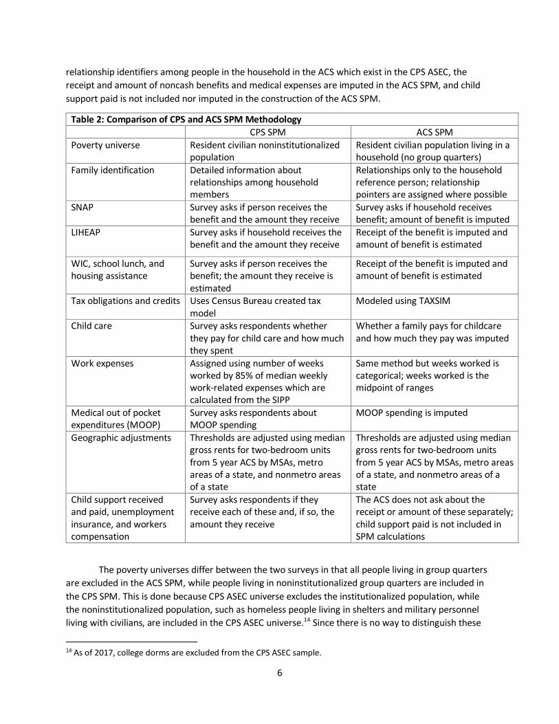
relationship identifiers among people in the household in the ACS which exist in the CPS ASEC, the receipt and amount of noncash benefits and medical expenses are imputed in the ACS SPM, and child support paid is not included nor imputed in the construction of the ACS SPM.

Table 2: Comparison of CPS and ACS SPM Methodology CPS SPM ACS SPM

Poverty universe Resident civilian noninstitutionalized population

Resident civilian population living in a household (no group quarters)

Family identification Detailed information about relationships among household members

Relationships only to the household reference person; relationship pointers are assigned where possible

SNAP Survey asks if person receives the benefit and the amount they receive

Survey asks if household receives benefit; amount of benefit is imputed

LIHEAP Survey asks if household receives the benefit and the amount they receive

Receipt of the benefit is imputed and amount of benefit is estimated

WIC, school lunch, and housing assistance

Survey asks if person receives the benefit; the amount they receive is estimated

Receipt of the benefit is imputed and amount of benefit is estimated

Tax obligations and credits Uses Census Bureau created tax model

Modeled using TAXSIM

Child care Survey asks respondents whether they pay for child care and how much they spent

Whether a family pays for childcare and how much they pay was imputed

Work expenses Assigned using number of weeks worked by 85% of median weekly work-related expenses which are calculated from the SIPP

Same method but weeks worked is categorical; weeks worked is the midpoint of ranges

Medical out of pocket expenditures (MOOP)

Survey asks respondents about MOOP spending

MOOP spending is imputed

Geographic adjustments Thresholds are adjusted using median gross rents for two-bedroom units from 5 year ACS by MSAs, metro areas of a state, and nonmetro areas of a state

Thresholds are adjusted using median gross rents for two-bedroom units from 5 year ACS by MSAs, metro areas of a state, and nonmetro areas of a state

Child support received and paid, unemployment insurance, and workers compensation

Survey asks respondents if they receive each of these and, if so, the amount they receive

The ACS does not ask about the receipt or amount of these separately; child support paid is not included in SPM calculations

The poverty universes differ between the two surveys in that all people living in group quarters are excluded in the ACS SPM, while people living in noninstitutionalized group quarters are included in the CPS SPM. This is done because CPS ASEC universe excludes the institutionalized population, while the noninstitutionalized population, such as homeless people living in shelters and military personnel living with civilians, are included in the CPS ASEC universe.14 Since there is no way to distinguish these

14 As of 2017, college dorms are excluded from the CPS ASEC sample.

7

groups from other group quarters residents in the ACS PUMS, the ACS sample is limited to people living in households.

Family identification is much more difficult in the ACS because while there is detailed information about relationships among household members in the CPS ASEC, the ACS only has information about people’s relationship to the household reference person. For instance, individuals in unrelated subfamilies15 in the CPS ASEC are assumed to pool resources while in the ACS anyone not related to the household reference person is treated as an unrelated individual.

For this project, the Census Bureau developed a method to assign parent and spouse identifiers based on rules used by the University of Minnesota’s IPUMS project.16 Whenever family relationships are unclear, the method uses age, marital status, and the order in which individuals are listed on the ACS form to assign family relationships. These identifiers allow for the creation of some unrelated subfamilies. All individuals aged 15 or older who are unrelated to the household reference person, are not a cohabiting partner of the reference person, are not a foster child under the age of 22, and who are not assigned an identifier based on IPUMs criteria are considered unrelated individuals.

The value of five noncash benefits are added to cash income in order to compute the SPM. The CPS ASEC asks questions about whether or not people received each of these benefits and asks about the amount received from SNAP and LIHEAP. However, the ACS only asks about whether the household received SNAP benefits in the past year and does not ask about the amount of SNAP benefits received or any questions about the other four noncash benefits. Therefore, receipt of four of the noncash benefits as well as the amounts of all five noncash benefits have to be imputed or estimated in the ACS.

CPS ASEC vs. ACS: Differences in Resources

Data from the CPS ASEC are used to model ACS program participation in WIC, school lunch, housing assistance, and LIHEAP using a logistic regression model. Data from the CPS ASEC is also used to model the benefit amount for SNAP and LIHEAP using a predictive means match. All amounts are imputed at the SPM resource unit level. Values for WIC, school lunch, and housing assistance are then allocated based on programmatic data on benefit levels in the same way that values are assigned in the CPS ASEC (see appendix of Fox 2019 for details). 17

In Table 3, average income for SPM units with income greater than zero is presented for four different types of income. Public assistance income, Social Security income and total income is lower and Supplemental Security Income (SSI) is higher in the ACS than in the CPS ASEC.18

15 Unrelated subfamilies are families in a household who are not related to the household reference person. 16 Steven Ruggles, Sarah Flood, Ronald Goeken, Josiah Grover, Erin Meyer, Jose Pacas and Matthew Sobek. IPUMS USA: Version 10.0 [dataset]. Minneapolis, MN: IPUMS, 2020. https://doi.org/10.18128/D010.V10.0 17 For more details on the imputation and the predictive means match, see https://www.census.gov/content/dam/Census/library/working-papers/2015/demo/SEHSD-WP2015-09.pdf. 18 Previous work done at Census has shown that income is lower in the ACS than in the CPS ASEC: https://www.census.gov/content/dam/Census/library/working-papers/2015/demo/SEHSD-WP2015-01.pdf.

8

Table 3: Comparison of Conditional Mean Annual Benefit Amounts and Total Income for SPM units between the ACS and CPS ASEC: 2017 (in thousands of dollars) CPS ASEC ACS Difference (ACS – CPS ASEC) Public Assistance Income 3,403 2,930 *-473 Social Security Income 19,970 18,470 *-1,500 Supplemental Security Income 8,553 9,281 *728 Total Income 85,090 79,310 *-5,780 Note: Total income includes public assistance, Social Security, SSI, and other income sources. * Differences are statistically significant at the 90 percent confidence level. Source: U.S. Census Bureau, 2018 Current Population Survey Annual Social and Economic Supplement and 2017 American Community Survey.

In Figure 1, the amount of income added to resources by different programs is presented for the ACS and the CPS ASEC for 2017. In aggregate, SNAP added more to resources in the ACS than in the CPS ASEC, while housing subsidies and WIC added more to resources in the CPS ASEC than in the ACS. The differences in total resources added for school lunch, LIHEAP, and the Earned Income Tax Credit (EITC) were not statistically significant.

For the CPS SPM, tax obligations and credits are modeled using a tax calculator developed by the Census Bureau that uses CPS ASEC data enhanced with data from a statistical match to Internal Revenue Service data. Since this model does not exist for the ACS, the NBER’s TAXSIM program is used.19 TAXSIM calculates federal and state tax liability from survey data. The version used in this paper, TAXSIM 27, requires 27 inputs including state of residence, year of filing, marital status, ages of the primary taxpayer and spouse, number of dependents, and wages and income. A 2016 Urban Institute

19 TAXSIM is a program that calculates federal and state tax liabilities from survey data. See http://users.nber.org/~taxsim/ for more information.

SNAP* Housingsubsidies* School lunch LIHEAP WIC* EITC

ACS 37.6 21.0 14.7 2.0 2.1 42.0CPS 31.0 27.7 14.6 1.9 2.6 42.7

0

10

20

30

40

50

Aggr

egat

e Va

lue

(in B

illio

ns)

Figure 1: Aggregate Amounts Added to Resources - 2017

* Differences are statistically significant at 90 percent confidence level.Source: U.S. Census Bureau, 2017 American Community Survey and 2018 Current Population Survey Annual Social and Economic Supplement.

9

report found that using the Census tax model or TAXSIM to model taxes has little effect on the SPM rate.20

There are several issues which make running TAXSIM using ACS data challenging:

• Tax filing units need to be formed. This is challenging in the ACS due to the minimal relationship data available in the survey. Using relationship criteria developed by IPUMS, parental and spousal identifiers were created in order to identify the detailed familial relationships needed to form tax units.

• There is no information in the ACS about whether or not the respondent filed taxes. • There are a number of income variables that TAXSIM asks for which are not available in the ACS.

These are set to zero: mortgage deductions, dividends, capital gains, unemployment, other miscellaneous items, non-property income, and interest received.

In the CPS ASEC, respondents were asked if they paid for child care while working and how much they spent. Since there are no questions about child care in the ACS, a logistic method is used to determine which units pay for childcare and a predicted means matching method is used to impute a weekly child care amount to each unit paying for child care using the CPS ASEC. This is then multiplied by the number of weeks worked by the reference person, spouse, or cohabiting partner who has the least number of weeks worked.21

Similar methods are used in the CPS ASEC and the ACS to calculate work expenses. First, median weekly work expenses are derived from the Survey of Income and Program Participation (SIPP). The number of weeks worked is multiplied by 85 percent of median weekly expenses to calculate annual individual work expenses. Individual work expenses are capped at individual earnings. Once again, due to the categorical nature of weeks worked in the ACS, work expenses are measured less precisely in the ACS than in the CPS ASEC. Combined child care and work expenses are capped following the same procedure as the CPS ASEC. They are not allowed to exceed the earnings of the household reference person, spouse, or cohabiting partner with the lowest earnings.

The CPS ASEC has specific questions about medical out of pocket expenditures (MOOP). There are no questions about medical expenses in the ACS so CPS ASEC data on MOOP are used to model expenditures of health insurance premiums and other medical expenses in the ACS.22

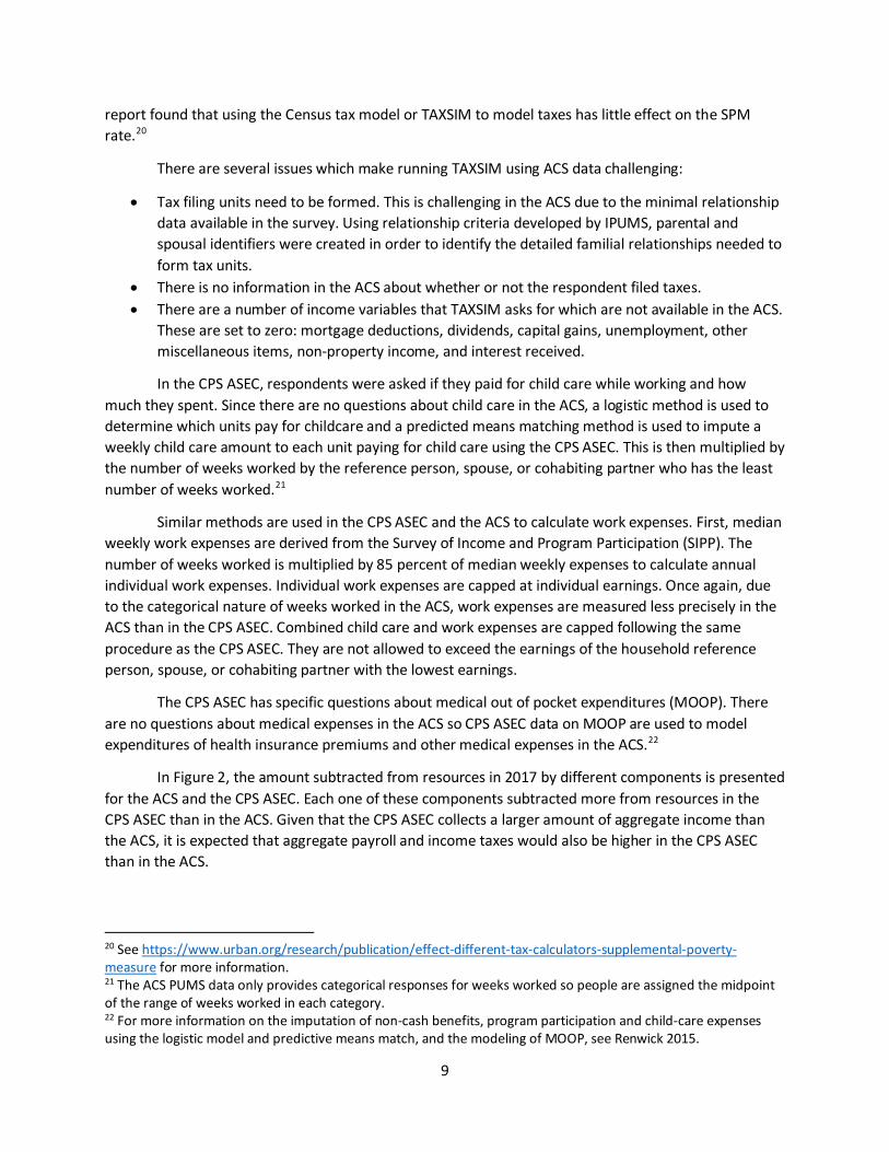
In Figure 2, the amount subtracted from resources in 2017 by different components is presented for the ACS and the CPS ASEC. Each one of these components subtracted more from resources in the CPS ASEC than in the ACS. Given that the CPS ASEC collects a larger amount of aggregate income than the ACS, it is expected that aggregate payroll and income taxes would also be higher in the CPS ASEC than in the ACS.

20 See https://www.urban.org/research/publication/effect-different-tax-calculators-supplemental-poverty-measure for more information. 21 The ACS PUMS data only provides categorical responses for weeks worked so people are assigned the midpoint of the range of weeks worked in each category. 22 For more information on the imputation of non-cash benefits, program participation and child-care expenses using the logistic model and predictive means match, and the modeling of MOOP, see Renwick 2015.

10

The CPS ASEC asks respondents about child support paid and received, unemployment insurance payments, and workers compensation payments. The ACS does not ask questions about child support paid; and income from unemployment, workers compensation, and child support received are reported in broader aggregated income categories that cannot be disentangled individually, but are included in overall resources.

While these additions and subtractions are included in the resource side of the ACS SPM, corresponding modifications are made to the threshold side as well. Despite differences in reference periods, base thresholds for the ACS SPM are identical to the CPS SPM, using the same base threshold for all respondents in a given year, regardless of interview month.23 Similar to the CPS SPM, the housing portion of the SPM thresholds are adjusted for geographic differences in housing costs. The adjustments are based on 5-year ACS estimates of median gross rents for two-bedroom units with complete kitchen and plumbing facilities. For the CPS ASEC, medians were calculated for the metropolitan areas large enough to be identified on the public-use CPS ASEC file, for nonmetropolitan areas of each state, and for a combination of all smaller metropolitan areas within a state. Since the ACS PUMS identifies PUMAs24 but does not identify metropolitan statistical areas, a PUMA-MSA crosswalk was used to create MSAs and nonmetropolitan areas of each state in the ACS in order to calculate the geographic adjustments.

Results

In the remainder of the paper, the results of the ACS SPM are presented in a number of different ways. First, the ACS SPM results are displayed over time, for the years 2014 through 2017, and

23 Future research could examine a linearly-interpolated threshold that varies depending on which month the ACS respondent was interviewed. 24 PUMAs are geographic areas of 100,000 or more people located within a state. These may be smaller than MSAs which means there may be multiple PUMAs within a single MSA.

Federaltaxes* FICA* State taxes* Work

expenses* Child care* Medical*

ACS 1322.0 583.4 301.3 262.7 35.4 616.7CPS 1382.4 628.1 343.9 275.9 51.6 635.3

0200400600800

1000120014001600

Aggr

egat

e Va

lue

(in B

illio

ns)

Figure 2: Aggregate Amounts Subtracted from Resources - 2017

* Differences are statistically significant at 90 percent confidence level.Source: U.S. Census Bureau, 2017 American Community Survey and 2018 Current Population Survey Annual Social and Economic Supplement.

11

compared to the CPS SPM.25 Second, the ACS SPM estimates are compared to the ACS OPM estimates. Third, ACS SPM estimates are shown by population subgroups and marginal impacts are shown for various programs.

ACS SPM vs. CPS SPM

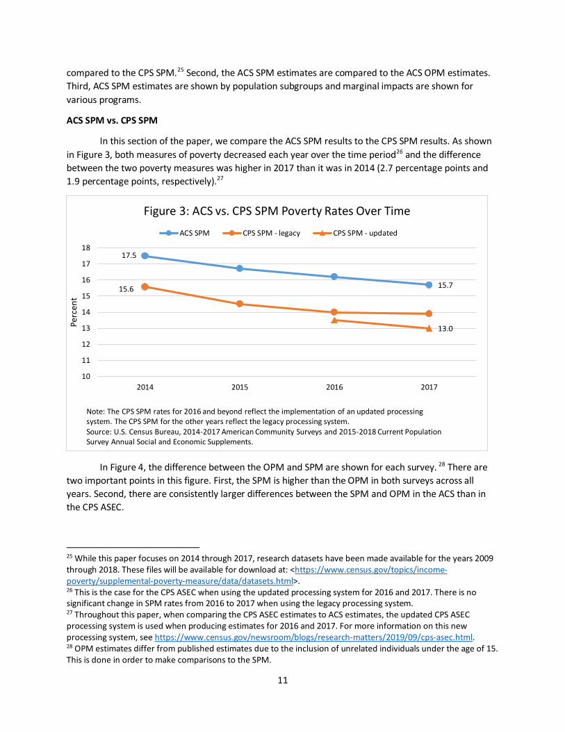
In this section of the paper, we compare the ACS SPM results to the CPS SPM results. As shown in Figure 3, both measures of poverty decreased each year over the time period26 and the difference between the two poverty measures was higher in 2017 than it was in 2014 (2.7 percentage points and 1.9 percentage points, respectively).27

In Figure 4, the difference between the OPM and SPM are shown for each survey. 28 There are two important points in this figure. First, the SPM is higher than the OPM in both surveys across all years. Second, there are consistently larger differences between the SPM and OPM in the ACS than in the CPS ASEC.

25 While this paper focuses on 2014 through 2017, research datasets have been made available for the years 2009 through 2018. These files will be available for download at: <https://www.census.gov/topics/income-poverty/supplemental-poverty-measure/data/datasets.html>. 26 This is the case for the CPS ASEC when using the updated processing system for 2016 and 2017. There is no significant change in SPM rates from 2016 to 2017 when using the legacy processing system. 27 Throughout this paper, when comparing the CPS ASEC estimates to ACS estimates, the updated CPS ASEC processing system is used when producing estimates for 2016 and 2017. For more information on this new processing system, see https://www.census.gov/newsroom/blogs/research-matters/2019/09/cps-asec.html. 28 OPM estimates differ from published estimates due to the inclusion of unrelated individuals under the age of 15. This is done in order to make comparisons to the SPM.

17.5

15.715.6

13.0

10

11

12

13

14

15

16

17

18

2014 2015 2016 2017

Perc

ent

Figure 3: ACS vs. CPS SPM Poverty Rates Over Time

ACS SPM CPS SPM - legacy CPS SPM - updated

Note: The CPS SPM rates for 2016 and beyond reflect the implementation of an updated processing system. The CPS SPM for the other years reflect the legacy processing system.Source: U.S. Census Bureau, 2014-2017 American Community Surveys and 2015-2018 Current Population Survey Annual Social and Economic Supplements.

12

In Figure 5, the difference between ACS SPM and CPS SPM are shown for different demographic groups in 2017. The ACS SPM is either higher or not statistically different from the CPS SPM for all demographic groups shown in Figure 5. By age category, the SPM is higher in the ACS than in the CPS ASEC for the under age 18 years category and age 18 to 64 years category, but the difference between the ACS SPM and CPS SPM is not statistically significant for the age 65 years and over category. Similarly, the difference in SPM rates between the ACS and the CPS ASEC is not statistically significant for cohabiting partners and male reference person SPM units, while the ACS SPM is higher than the CPS SPM for all other SPM unit types. Finally, the ACS SPM is higher than CPS SPM for all people age 25 years and over for each education category, though the difference is significantly less for people with a college degree than for people without a college degree.

2.2 2.22.4 2.5

0.81.0

0.7 0.7

2014 2015 2016 2017

SPM

-O

PMFigure 4: Percentage Point Difference Between SPM and

OPM Poverty Rates by YearACS CPS

Source: U.S. Census Bureau, 2014-2017 American Comunity Surveys and 2015-2018 Current Population Survey Annual Social and Economic Supplements.

13

0 5 10 15 20 25 30 35

Percent

Figure 5: Percentage of People in Poverty Using the SPM: ACS vs. CPS 2017

CPS ACS

* An asterisk preceding an estimate indicates that the difference between ACS and CPS ASEC estimate is statistically different from zero at the 90 percent confidence level. Note: Hollow markers signify that the ACS and CPS ASEC estimates are not statistically different at the 90 percent confidence level. Source: U.S. Census Bureau, 2017 American Community Survey and 2018 Current Population Survey Annual Social and Economic Supplement.

CPS ACS Diff.

All people 13.0 15.7 *2.7

Sex

Male 12.3 14.7 *2.4

Female 13.7 16.6 *2.9

Age

Under 18 years 14.2 17.6 *3.4

18 to 64 years 12.4 15.4 *3.0

65 years and over 13.6 13.9 0.3

Type of SPM Unit

Married Couple 7.6 9.7 *1.9

Cohabiting partners 14.9 15.1 0.2

Female reference person 25.3 29.9 *4.6

Male reference person 17.3 17.9 0.6

Unrelated individuals 22.3 27.5 *5.2

Race and Hispanic Origin

White 11.5 13.0 *1.5

White, not Hispanic 9.0 11.2 *2.2

Black 20.6 23.6 *3.0

Asian 14.0 18.4 *4.4

Hispanic (any race) 20.5 24.1 *3.6

Educational Attainment, 25 years and over

No high school diploma 27.4 30.1 *2.7

High school, no college 15.2 17.3 *2.1

Some college 10.2 12.1 *1.9

Bachelor's degree or higher 5.8 6.3 *0.5

Work Experience, 18 years and over

All workers 7.4 10.6 *3.2

Worked full-time, year-round 4.5 5.4 *0.9

Less than full-time, year-round 15.0 21.7 *6.7

Did not work at least 1 week 29.0 33.0 *4.0

14

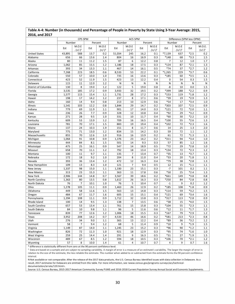
In Figure 6 and Figure 7, states are broken up into quintiles by SPM poverty rate.29 This is done separately for the ACS in Figure 6, and the CPS ASEC in Figure 7, so the bottom quintile and top quintile of states can be compared between the two surveys more readily.30 There are seven states in the bottom quintile for SPM rates in common for both surveys: Iowa, Kansas, Minnesota, Nebraska, New Hampshire, Vermont, and Wisconsin. Similarly, there are eight states, Arizona, California, Florida, Georgia, Louisiana, Mississippi, New Mexico, and New York, and the District of Columbia in the top quintile for SPM rates in common for both sets of estimates. While the magnitudes of the SPM rates differ, the South has relatively higher poverty rates and the Midwest and parts of the West have relatively low SPM rates using both surveys.

29 Three-year averages are used because while a single year of the ACS is representative at the state and sub-state level, the Census Bureau recommends the use of three-year averages when calculating state-level poverty rates using the CPS ASEC. 30 In the appendix, SPM poverty rates using the ACS and CPS ASEC by state are shown in Table A-4.

15

Similar to the difference between the two surveys nationally, the three-year average ACS SPM is higher than the three-year average CPS SPM in 40 states. In three of those states (California, New York, and Rhode Island), the difference in SPM rates between the two surveys is significantly larger than the 3-year average national difference in SPM rates. The difference in SPM rates is not statistically significant in 9 states and the District of Columbia.

OPM vs. SPM (ACS)

In this section of the paper, we compare the ACS SPM results to the ACS OPM. As shown in Figure 8, both measures of poverty decrease each year over the time period and the difference between the two poverty measures is relatively stable, with the SPM between 2.2 and 2.5 percentage points higher than the OPM.

16

In Figure 9, differences between the ACS OPM and the ACS SPM are shown by different demographic groups for the year 2017. The SPM is higher than the OPM for both males and females but the difference in the two rates is larger for males. The SPM rate is higher than the OPM for people aged 18 years and over while the OPM rate is higher than the SPM for people under age 18. Furthermore, there is a larger difference in poverty rates across the two measures for the 65 years and over population than for the 18 to 64 year old population.

The SPM rate is higher than the OPM rate for all types of SPM units except for cohabiting partners. When the SPM is higher than the OPM, the largest difference in rates is for SPM units with a male reference person while the smallest difference is for SPM units with a female reference person. By race, SPM rates are higher than OPM rates across all groups, with the largest difference in poverty rates for Asians and the smallest difference for Blacks.

By educational attainment, SPM rates are higher than OPM rates across all groups, and the difference between the SPM rate and the OPM rate decreases as the level of education increases. For work experience among 18 to 64 year olds, SPM rates were consistently higher than OPM rates, with the largest difference in poverty rates for people who worked less than full-time, year-round while the smallest difference for people who did not work at least one week.

17.5

15.715.3

13.2

12.0

13.0

14.0

15.0

16.0

17.0

18.0

2014 2015 2016 2017

Figure 8: SPM vs. OPM Poverty Rates using the ACS Over Time

ACS SPM ACS OPM

Source: U.S. Census Bureau, 2014-2017 American Community Surveys.

17

0 5 10 15 20 25 30 35

Percent

Figure 9: Percentage of People in Poverty by Different Poverty Measures in the ACS: 2017

OPM SPM

OPM SPM DifferenceAll people 13.2 15.7 *2.5

Sex

Male 11.9 14.7 *2.8

Female 14.4 16.6 *2.2AgeUnder 18 years 18.2 17.6 *-0.618 to 64 years 12.3 15.4 *3.1

65 years and over 9.0 13.9 *4.9

Type of SPM UnitMarried Couple 5.8 9.7 *3.9Cohabiting partners 26.9 15.1 *-11.8

Female reference person 27.9 29.9 *2.0

Male reference person 13.4 17.9 *4.4

Unrelated individuals 23.9 27.5 *3.6Race and Hispanic OriginWhite 11.0 13.0 *2.1

White, not Hispanic 9.5 11.2 *1.7

Black 22.5 23.6 *1.1

Asian 11.0 18.4 *7.4Hispanic (any race) 19.2 24.1 *4.9Educational Attainment, 25 years and over

No high school diploma 24.4 30.1 *5.7

High school, no college 13.3 17.3 *4.0

Some college 9.3 12.1 *2.8

Bachelor's degree or higher 4.2 6.3 *2.1Work Experience, 18 to 64 yearsAll workers 7.4 10.8 *3.3

Worked full-time, year-round 2.6 5.6 *2.9

Less than full-time, year-round 17.8 22.0 *4.2

Did not work at least 1 week 31.1 33.2 *2.1

* An asterisk preceding an estimate indicates difference between SPM and OPM is statistically different from zero at the 90 percentconfidence level.Source: U.S. Census Bureau, 2017 American Community Survey.

18

In Figure 10, the difference between the ACS SPM and ACS OPM are shown by state.31 In 25 states and the District of Columbia, the SPM rate was higher than the OPM rate. The SPM rate was lower than the OPM rate in 11 states and the difference between the SPM rate and the OPM rate was not statistically significant in 13 states.

ACS SPM

The SPM decreased each year from 2014 to 2017. By age category, this same decline was only observed for people ages 18 to 64. SPM rates for people under age 18 declined each year from 2014 to 2016,32 while for people ages 65 and over, the SPM does not move in a consistent direction. For each year, the SPM was highest for people under age 18 and lowest for people age 65 and older.

31 A table showing ACS OPM and ACS SPM estimates by state for 2017 is in the appendix (Table A-1). 32 The change from 2016 to 2017 was not statistically significant.

19

In Figure 12, the ACS SPM is shown by state for 2017.33 In the appendix to this paper, there is a table showing state level SPM estimates for 2014 to 2017 (Appendix Table A-2). There are also tables showing state level SPM estimates by age group for 2014 to 2017 (Appendix Tables A-3A, A-3B, A-3C, and A-3D).

In 2017, 12 states and the District of Columbia had ACS SPM rates higher than the national ACS SPM rate of 15.7 percent, 33 states had ACS SPM rates lower than the national rate, and four states34 had ACS SPM rates not significantly different than the national rate. The lowest ACS SPM rates are in the Midwest and New England, while the highest ACS SPM rates are concentrated in the South and Southwest.

33 Census guidance recommends using three-year averages when generating state-level estimates in the CPS ASEC due to sample size. As such, the CPS SPM can only be produced for states using 3 years of data since one year of CPS ASEC data is only representative at the national level. However, one year of ACS data is representative at both the state level and the national level. 34 Kentucky, Nevada, North Carolina, and South Carolina.

17.519.8

17.5

14.0

16.718.7

16.7

13.4

16.217.9

16.113.9

15.717.6

15.413.9

All people under 18 years 18 to 64 years 65 years and over

Figure 11: ACS SPM Poverty Rates Over Time

2014 2015 2016 2017

Source: U.S. Census Bureau, 2014-2017 American Community Surveys.

20

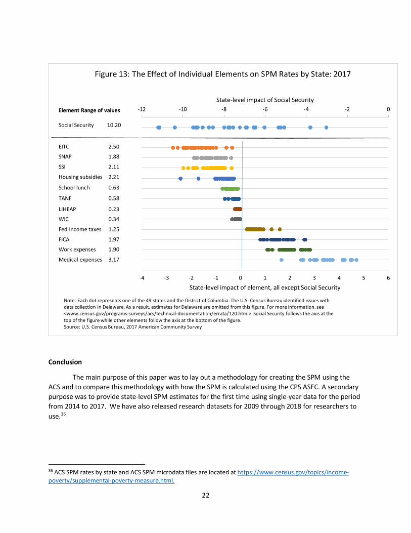
One benefit of the SPM is that it allows an examination of the impact of policies and programs on poverty rates. We can individually subtract the value of programs or cost of expenses one at a time and determine the marginal impact of each on the ACS SPM. This counterfactual exercise assumes no behavioral changes and does not attempt to estimate the causal impact of each element. This is done in Table 4 for all people and for different age categories and in Figure 13 by state. The estimates in the table are the percentage point difference in SPM rates, holding all else equal, when excluding the element in question. A negative value means the SPM rate would have been higher without the benefit and a positive value means the SPM rate would have been lower without the expense.

Social Security had the largest effect on the overall SPM rate, reducing poverty by 7.38 percentage points. All other resource additions reduced the SPM rate by less than 2.0 percentage points. Most of this is due to the targeting of Social Security benefits to people age 65 and over. Social Security reduced poverty for this group by 31.18 percentage points. In other words, approximately 45 percent of those ages 65 and older would have been in poverty without Social Security. However, Social Security only reduced the child SPM rate by 1.70 percentage points. Tax credits and SNAP were more important programs for reducing child poverty.

The element that increased overall SPM rates the most was medical expenses. This was true for all age categories but was the highest for those ages 65 and older, followed by children, and then those

21

ages 18 to 64. Work expenses and FICA had a larger effect on children than on the other two age groups while federal income tax had a larger effect on those ages 18 to 64 than on the other two age group.

Table 4: Effect of Individual Elements on SPM Rates: 2017

Element All People Under 18 years 18 to 64 years 65 years and over

Estimate Margin of error

Estimate Margin of error

Estimate Margin of error

Estimate Margin of error

Total SPM rate 15.69 0.09 17.63 0.15 15.40 0.09 13.94 0.12 ADDITIONS

Social Security -7.38 0.04 -1.70 0.05 -3.51 0.03 -31.18 0.15 Refundable tax credits (EITC) -1.92 0.03 -4.24 0.08 -1.49 0.03 -0.15 0.01 SNAP -1.21 0.03 -2.24 0.06 -0.97 0.02 -0.64 0.02 SSI -1.09 0.02 -0.76 0.03 -1.15 0.02 -1.36 0.04 Housing subsidies -0.66 0.02 -0.93 0.04 -0.52 0.02 -0.82 0.03 School lunch -0.41 0.01 -1.02 0.04 -0.28 0.01 -0.04 0.01 TANF/general assistance -0.20 0.01 -0.35 0.02 -0.17 0.01 -0.11 0.01 LIHEAP -0.05 0.005 -0.07 0.01 -0.04 0.004 -0.05 0.01 WIC -0.08 0.01 -0.20 0.02 -0.06 0.01 -0.005 0.002

SUBTRACTIONS Federal income tax 0.68 0.02 0.69 0.03 0.79 0.02 0.20 0.01 FICA 1.74 0.03 2.38 0.06 1.85 0.03 0.39 0.02 Work expenses 2.19 0.03 3.09 0.07 2.28 0.04 0.51 0.02 Medical expenses 3.70 0.04 3.90 0.08 3.30 0.04 5.01 0.07 Note: All estimates statistically different from zero t the 90 percent confidence level. Data are based on a sample and are subject to sampling variability. A margin of error is a measure of an estimate’s variability. The larger the margin of error in relation to the size of the estimate, the less reliable the estimate. This number when added to or subtracted from the estimate forms the 90 percent confidence interval. Source: U.S. Census Bureau, 2017 American Community Survey.

In Figure 13, the effects of the individual elements on the SPM rate are shown for each state and the District of Columbia. Each state and the District of Columbia are represented as a separate dot in order to show the range of effects these elements have on the SPM rate in different states.35

West Virginia was among the states most impacted by Social Security and Alaska was among the states least impacted by Social Security. For the other elements, there is a spread among the states, but the lack of precision makes it difficult to truly rank the state estimate in any meaningful way. The values for the individual effects by state are displayed in appendix tables (Tables A-5A and A-5B).

35 Since the impact of Social Security is so much larger than the other elements, the impact of Social Security is shown on a different axis: Social Security is measured on the top axis and the other elements are measured on the bottom axis.

22

Conclusion

The main purpose of this paper was to lay out a methodology for creating the SPM using the ACS and to compare this methodology with how the SPM is calculated using the CPS ASEC. A secondary purpose was to provide state-level SPM estimates for the first time using single-year data for the period from 2014 to 2017. We have also released research datasets for 2009 through 2018 for researchers to use.36

36 ACS SPM rates by state and ACS SPM microdata files are located at https://www.census.gov/topics/income-poverty/supplemental-poverty-measure.html.

-12 -10 -8 -6 -4 -2 0

-4 -3 -2 -1 0 1 2 3 4 5 6

State-level impact of Social Security

State-level impact of element, all except Social Security

Figure 13: The Effect of Individual Elements on SPM Rates by State: 2017

Element Range of values

Social Security 10.20

EITC 2.50

SNAP 1.88

SSI 2.11

Housing subsidies 2.21

School lunch 0.63

TANF 0.58

LIHEAP 0.23

WIC 0.34

Fed Income taxes 1.25

FICA 1.97

Work expenses 1.90

Medical expenses 3.17

Note: Each dot represents one of the 49 states and the District of Columbia. The U.S. Census Bureau identified issues with data collection in Delaware. As a result, estimates for Delaware are omitted from this figure. For more information, see <www.census.gov/programs-surveys/acs/technical-documentation/errata/120.html>. Social Security follows the axis at the top of the figure while other elements follow the axis at the bottom of the figure. Source: U.S. Census Bureau, 2017 American Community Survey

23

References

Bohn, S., Danielson, C., Kimberlin, S., Mattingly, M., and Wimer, C., The California Poverty Measure 2012 Technical Appendices, Stanford Center on Poverty and Inequality. 2015, https://inequality.stanford.edu/sites/default/files/CPM_2012_appendices.pdf.

Chung, Y., Isaacs, J.B., Smeeding, T.M., Thornton, K.A., May 2012. Wisconsin Poverty Report: Policy

Context, Methodology, and Results for 2010, Part of the Wisconsin Poverty Project’s Fourth Annual Report Series. Institute for Research on Poverty University of Wisconsin Madison. https://www.irp.wisc.edu/wp/wp-content/uploads/2018/05/WIPovPolicyContextMethodologyResults_May2012.pdf.

Fox, Liana, “The Supplemental Poverty Measure: 2018,” Current Population Reports, P60-268, U.S.

Census Bureau, October 2019, available at < https://www.census.gov/content/dam/Census/library/publications/2019/demo/p60-268.pdf>

Fox, Liana, Jose Pacas, and Brian Glassman, “Using the American Community Survey (ACS) to Implement

a Supplemental Poverty Measure (SPM)”, Presented at ACS Data Users Conference, May 11, 2017.

New York City Center for Economic Opportunity (NYC-CEO), April 2019a, New York City Government Poverty Measure 2017, An Annual Report. Appendix B Deriving a Poverty Threshold for New York City https://www1.nyc.gov/assets/opportunity/pdf/NYCgovPoverty2019_Appendix_B.pdf

Renwick, Trudi, “Using the American Community Survey (ACS) to Implement a Supplemental Poverty

Measure (SPM)”, SEHSD Working Paper Number 2015-09, U.S. Census Bureau, 2015.

Renwick, Trudi, Kathleen Short, Ale Bishaw, and Charles Hokayem, “Using the American Community Survey (ACS) to implement a Supplemental Poverty Measure, SEHSD Working Paper Number 2012-10, U.S. Census Bureau, 2012.

Ruggles, Steven, Sarah Flood, Ronald Goeken, Josiah Grover, Erin Meyer, Jose Pacas and Matthew Sobek. IPUMS USA: Version 10.0 [dataset]. Minneapolis, MN: IPUMS, 2020. https://doi.org/10.18128/D010.V10.0

24

Appendix

Table A-1: Number (in thousands) and Percentage of People in Poverty by State using the ACS: 2017 ACS OPM1 ACS SPM Difference (SPM less OPM)

Number Percent Number Percent Number Percent

Total Est M.O.E. (+/-)2 Est

M.O.E. (+/-)2 Est

M.O.E. (+/-)2 Est

M.O.E. (+/-)2 Est

M.O.E. (+/-)2 Est

M.O.E. (+/-)2

United States 317,632 41,831 292 13.2 0.1 49,830 291 15.7 0.1 *7,999 187 *2.5 0.1 Alabama 4,756 790 28 16.6 0.6 777 26 16.3 0.5 -13 23 -0.3 0.5 Alaska 712 81 11 11.3 1.6 91 11 12.7 1.6 *10 9 *1.4 1.3 Arizona 6,861 1,002 31 14.6 0.4 1,141 34 16.6 0.5 *139 28 *2.0 0.4 Arkansas 2,919 467 21 16.0 0.7 424 22 14.5 0.8 *-43 18 *-1.5 0.6 California 38,719 5,025 90 13.0 0.2 8,154 84 21.1 0.2 *3,129 80 *8.1 0.2 Colorado 5,488 558 23 10.2 0.4 735 27 13.4 0.5 *177 19 *3.2 0.4 Connecticut 3,474 316 19 9.1 0.5 423 25 12.2 0.7 *107 18 *3.1 0.5 Delaware N N N N N N N N N N N N N District of Columbia 654 103 8 15.7 1.2 121 10 18.5 1.6 *18 8 *2.8 1.3 Florida 20,556 2,838 63 13.8 0.3 3,855 60 18.8 0.3 *1,017 52 *4.9 0.3 Georgia 10,171 1,528 51 15.0 0.5 1,684 51 16.6 0.5 *155 31 *1.5 0.3 Hawaii 1,383 138 12 10.0 0.8 252 18 18.2 1.3 *114 16 *8.2 1.1 Idaho 1,687 219 16 13.0 1.0 205 15 12.2 0.9 *-14 13 *-0.8 0.8 Illinois 12,501 1,561 43 12.5 0.3 1,778 50 14.2 0.4 *217 40 *1.7 0.3 Indiana 6,480 866 33 13.4 0.5 894 30 13.8 0.5 *27 24 *0.4 0.4 Iowa 3,046 302 18 9.9 0.6 304 19 10.0 0.6 1 14 0.0 0.4 Kansas 2,833 334 17 11.8 0.6 327 17 11.5 0.6 -8 14 -0.3 0.5 Kentucky 4,322 742 26 17.2 0.6 701 24 16.2 0.6 *-40 17 *-0.9 0.4 Louisiana 4,555 900 34 19.8 0.7 897 32 19.7 0.7 -3 27 -0.1 0.6 Maine 1,300 145 12 11.1 0.9 134 11 10.3 0.8 *-11 9 *-0.9 0.7 Maryland 5,912 544 26 9.2 0.4 863 27 14.6 0.5 *319 23 *5.4 0.4 Massachusetts 6,609 668 27 10.1 0.4 896 27 13.6 0.4 *229 22 *3.5 0.3 Michigan 9,732 1,364 38 14.0 0.4 1,296 35 13.3 0.4 *-69 34 *-0.7 0.4 Minnesota 5,445 518 23 9.5 0.4 505 24 9.3 0.4 -13 19 -0.2 0.3 Mississippi 2,891 565 18 19.6 0.6 543 19 18.8 0.6 *-22 15 *-0.8 0.5 Missouri 5,939 778 25 13.1 0.4 778 25 13.1 0.4 0 22 0.0 0.4 Montana 1,022 126 10 12.3 1.0 125 10 12.2 1.0 -1 9 -0.1 0.8 Nebraska 1,868 196 15 10.5 0.8 183 14 9.8 0.7 *-13 12 *-0.7 0.6 Nevada 2,960 386 22 13.0 0.7 460 25 15.6 0.9 *75 20 *2.5 0.7 New Hampshire 1,300 95 9 7.3 0.7 127 11 9.7 0.9 *31 7 *2.4 0.5 New Jersey 8,823 842 30 9.5 0.3 1,271 32 14.4 0.4 *428 29 *4.9 0.3 New Mexico 2,045 397 17 19.4 0.9 347 16 17.0 0.8 *-50 14 *-2.4 0.7 New York 19,273 2,632 54 13.7 0.3 3,565 63 18.5 0.3 *933 54 *4.8 0.3 North Carolina 10,007 1,468 41 14.7 0.4 1,546 41 15.4 0.4 *78 33 *0.8 0.3 North Dakota 729 69 7 9.5 1.0 74 8 10.1 1.1 5 5 0.6 0.7 Ohio 11,341 1,550 38 13.7 0.3 1,378 36 12.2 0.3 *-171 34 *-1.5 0.3 Oklahoma 3,821 582 28 15.2 0.7 558 28 14.6 0.7 *-24 22 *-0.6 0.6 Oregon 4,053 522 23 12.9 0.6 597 25 14.7 0.6 *75 20 *1.8 0.5 Pennsylvania 12,382 1,527 43 12.3 0.3 1,699 47 13.7 0.4 *172 36 *1.4 0.3 Rhode Island 1,018 118 10 11.6 1.0 129 10 12.7 1.0 *12 9 *1.1 0.9 South Carolina 4,888 747 24 15.3 0.5 758 25 15.5 0.5 11 20 0.2 0.4 South Dakota 836 97 9 11.6 1.1 94 8 11.2 1.0 -3 7 -0.4 0.8 Tennessee 6,561 980 32 14.9 0.5 987 31 15.0 0.5 7 26 0.1 0.4 Texas 27,698 4,016 66 14.5 0.2 4,529 72 16.3 0.3 *513 49 *1.9 0.2 Utah 3,054 290 20 9.5 0.7 357 17 11.7 0.6 *67 17 *2.2 0.6 Vermont 599 65 9 10.9 1.4 74 11 12.4 1.8 *9 8 *1.5 1.3 Virginia 8,228 846 32 10.3 0.4 1,221 36 14.8 0.4 *375 25 *4.6 0.3 Washington 7,263 798 28 11.0 0.4 890 30 12.3 0.4 *93 25 *1.3 0.4 West Virginia 1,768 337 16 19.0 0.9 296 15 16.8 0.8 *-40 11 *-2.3 0.6 Wisconsin 5,650 608 28 10.8 0.5 586 27 10.4 0.5 -22 24 -0.4 0.4 Wyoming 565 67 8 11.8 1.4 65 8 11.5 1.3 -2 6 -0.3 1.0 * Difference is statistically different from zero at the 90 percent confidence level. 1 Differs from published estimates. Includes unrelated individuals under the age of 15. 2 Data are based on a sample and are subject to sampling variability. A margin of error is a measure of an estimate’s variability. The larger the margin of error in relation to the size of the estimate, the less reliable the estimate. This number when added to or subtracted from the estimate forms the 90 percent confidence interval. Z Represents or rounds to zero. N Not available or not comparable. After the release of the 2017 data products, the U.S. Census Bureau identified issues with data collection in Delaware. As a result, 2017 estimates for Delaware are omitted from this table. For more information, see <www.census.gov/programs-surveys/acs/technical-documentation/errata/120.html>. Source: U.S. Census Bureau, 2017 American Community Survey PUMS.

25

Table A-2: Number (in thousands) and Percentage of People in ACS SPM Poverty by State: 2014 to 2017 2017 2016 2015 2014

Number Percent Number Percent Number Percent Number Percent Est M.O.E

. (+/-)1 Est M.O.E. (+/-)1 Est M.O.E

. (+/-)1 Est M.O.E. (+/-)1 Est M.O.E

. (+/-)1 Est M.O.E. (+/-)1 Est M.O.E

. (+/-)1 Est M.O.E. (+/-)1

United States 49,830 291 15.7 0.1 50,950 302 16.2 0.1 52,324 321 16.7 0.1 54,477 327 17.5 0.1 Alabama 777 26 16.3 0.5 794 27 16.7 0.6 841 28 17.7 0.6 858 29 18.1 0.6 Alaska 91 11 12.7 1.6 84 10 11.8 1.4 87 12 12.2 1.7 88 14 12.4 2.0 Arizona 1,141 34 16.6 0.5 1,206 33 17.8 0.5 1,210 39 18.1 0.6 1,282 35 19.5 0.5 Arkansas 424 22 14.5 0.8 495 23 17.1 0.8 483 20 16.7 0.7 475 21 16.5 0.7 California 8,154 84 21.1 0.2 8,553 98 22.3 0.3 8,942 104 23.3 0.3 9,589 109 25.2 0.3 Colorado 735 27 13.4 0.5 732 26 13.5 0.5 739 27 13.8 0.5 744 28 14.2 0.5 Connecticut 423 25 12.2 0.7 409 21 11.8 0.6 437 22 12.6 0.6 418 20 12.0 0.6 Delaware N N N N 130 12 14.0 1.3 129 14 14.0 1.5 130 11 14.2 1.2 District of Columbia 121 10 18.5 1.6 129 10 20.1 1.5 116 9 18.4 1.4 113 10 18.3 1.7 Florida 3,855 60 18.8 0.3 3,943 55 19.5 0.3 3,991 58 20.1 0.3 4,122 75 21.2 0.4 Georgia 1,684 51 16.6 0.5 1,702 41 16.9 0.4 1,805 45 18.1 0.4 1,887 46 19.2 0.5 Hawaii 252 18 18.2 1.3 218 16 15.8 1.2 242 15 17.4 1.1 244 17 17.7 1.2 Idaho 205 15 12.2 0.9 207 15 12.5 0.9 227 16 14.0 1.0 239 16 14.9 1.0 Illinois 1,778 50 14.2 0.4 1,817 47 14.5 0.4 1,936 48 15.4 0.4 2,042 48 16.2 0.4 Indiana 894 30 13.8 0.5 880 26 13.6 0.4 929 30 14.4 0.5 943 32 14.7 0.5 Iowa 304 19 10.0 0.6 319 17 10.5 0.6 361 20 11.9 0.6 344 23 11.4 0.8 Kansas 327 17 11.5 0.6 335 18 11.9 0.6 331 20 11.7 0.7 362 20 12.8 0.7 Kentucky 701 24 16.2 0.6 742 29 17.2 0.7 684 27 15.9 0.6 697 23 16.3 0.5 Louisiana 897 32 19.7 0.7 870 29 19.1 0.6 882 34 19.4 0.7 872 28 19.3 0.6 Maine 134 11 10.3 0.8 156 15 12.0 1.2 164 12 12.7 0.9 162 12 12.5 0.9 Maryland 863 27 14.6 0.5 792 28 13.5 0.5 847 32 14.4 0.5 842 34 14.4 0.6 Massachusetts 896 27 13.6 0.4 882 28 13.5 0.4 968 30 14.8 0.5 933 32 14.4 0.5 Michigan 1,296 35 13.3 0.4 1,385 42 14.3 0.4 1,446 40 14.9 0.4 1,488 37 15.4 0.4 Minnesota 505 24 9.3 0.4 473 25 8.8 0.5 525 25 9.8 0.5 537 29 10.1 0.5 Mississippi 543 19 18.8 0.6 521 23 18.0 0.8 576 24 19.9 0.8 584 25 20.2 0.9 Missouri 778 25 13.1 0.4 790 29 13.3 0.5 808 30 13.7 0.5 877 30 14.9 0.5 Montana 125 10 12.2 1.0 133 9 13.2 0.9 148 13 14.7 1.3 156 14 15.7 1.4 Nebraska 183 14 9.8 0.7 213 14 11.5 0.8 217 13 11.8 0.7 202 12 11.1 0.7 Nevada 460 25 15.6 0.9 472 23 16.3 0.8 485 22 17.0 0.8 481 22 17.2 0.8 New Hampshire 127 11 9.7 0.9 119 11 9.2 0.9 117 11 9.1 0.8 130 11 10.1 0.9 New Jersey 1,271 32 14.4 0.4 1,320 44 15.1 0.5 1,398 43 15.9 0.5 1,428 35 16.3 0.4 New Mexico 347 16 17.0 0.8 357 19 17.5 1.0 384 23 18.8 1.1 389 21 19.0 1.0 New York 3,565 63 18.5 0.3 3,536 54 18.4 0.3 3,648 62 19.0 0.3 3,664 66 19.1 0.3 North Carolina 1,546 41 15.4 0.4 1,623 40 16.4 0.4 1,668 39 17.0 0.4 1,723 40 17.8 0.4 North Dakota 74 8 10.1 1.1 76 9 10.4 1.2 77 8 10.6 1.1 84 9 11.8 1.2 Ohio 1,378 36 12.2 0.3 1,483 41 13.1 0.4 1,527 43 13.5 0.4 1,651 41 14.6 0.4 Oklahoma 558 28 14.6 0.7 563 22 14.8 0.6 570 21 15.0 0.6 559 23 14.8 0.6 Oregon 597 25 14.7 0.6 591 23 14.8 0.6 626 23 15.9 0.6 679 28 17.5 0.7 Pennsylvania 1,699 47 13.7 0.4 1,735 46 14.0 0.4 1,701 48 13.7 0.4 1,822 44 14.7 0.4 Rhode Island 129 10 12.7 1.0 136 11 13.5 1.1 147 12 14.5 1.1 156 12 15.4 1.1 South Carolina 758 25 15.5 0.5 737 24 15.3 0.5 788 27 16.5 0.6 832 28 17.7 0.6 South Dakota 94 8 11.2 1.0 98 10 11.8 1.2 96 10 11.6 1.2 99 9 12.1 1.0 Tennessee 987 31 15.0 0.5 1,014 30 15.6 0.5 1,017 35 15.8 0.5 1,118 32 17.5 0.5 Texas 4,529 72 16.3 0.3 4,621 76 17.0 0.3 4,413 72 16.4 0.3 4,651 63 17.6 0.2 Utah 357 17 11.7 0.6 374 18 12.5 0.6 365 22 12.4 0.8 387 22 13.3 0.8 Vermont 74 11 12.4 1.8 69 8 11.5 1.3 61 8 10.2 1.3 74 8 12.4 1.3 Virginia 1,221 36 14.8 0.4 1,249 36 15.3 0.4 1,266 40 15.6 0.5 1,293 37 16.0 0.5 Washington 890 30 12.3 0.4 919 31 12.9 0.4 954 33 13.6 0.5 1,016 30 14.7 0.4 West Virginia 296 15 16.8 0.8 283 16 15.9 0.9 293 18 16.3 1.0 282 17 15.7 0.9 Wisconsin 586 27 10.4 0.5 598 26 10.6 0.5 599 28 10.7 0.5 661 29 11.8 0.5 Wyoming 65 8 11.5 1.3 64 7 11.2 1.1 54 7 9.4 1.2 68 8 11.9 1.4 1 Data are based on a sample and are subject to sampling variability. A margin of error is a measure of an estimate’s variability. The larger the margin of error in relation to the size of the estimate, the less reliable the estimate. This number when added to or subtracted from the estimate forms the 90 percent confidence interval. N Not available or not comparable. After the release of the 2017 data products, the U.S. Census Bureau identified issues with data collection in Delaware. As a result, 2017 estimates for Delaware are omitted from this table. For more information, see <www.census.gov/programs-surveys/acs/technical-documentation/errata/120.html>. Source: U.S. Census Bureau, 2014-2017 American Community Survey PUMS.

26

Table A-3A: Number (in thousands) and Percentage of People in SPM Poverty by Age Groups by State: 2017 Under age 18 Age 18 to 64 Age 65 and over

Number Percent Number Percent Number Percent Est M.O.E

. (+/-)1 Est M.O.E. (+/-)1 Est M.O.E.

(+/-)1 Est M.O.E. (+/-)1 Est M.O.E

. (+/-)1 Est M.O.E. (+/-)1

United States 12,933 116 17.6 0.2 30,030 178 15.4 0.1 6,867 56 13.9 0.1 Alabama 206 11 18.9 1.0 472 18 16.3 0.6 99 6 12.7 0.8 Alaska 26 5 14.0 2.9 55 8 12.3 1.7 10 2 12.0 3.0 Arizona 314 14 19.3 0.9 678 23 16.7 0.6 148 8 12.6 0.7 Arkansas 108 11 15.3 1.6 258 12 14.9 0.7 58 5 12.0 1.0 California 2,172 36 24.1 0.4 4,902 56 20.2 0.2 1,080 19 20.1 0.4 Colorado 180 12 14.3 1.0 460 18 13.2 0.5 96 6 12.6 0.7 Connecticut 101 10 13.6 1.3 260 16 12.1 0.7 62 5 10.8 0.8 Delaware N N N N N N N N N N N N District of Columbia 31 6 24.8 4.5 76 7 17.0 1.5 14 2 17.3 2.7 Florida 910 28 21.7 0.7 2,269 39 18.5 0.3 676 18 16.4 0.4 Georgia 467 25 18.6 1.0 1,020 29 16.2 0.5 197 9 14.4 0.6 Hawaii 66 7 21.9 2.4 143 11 17.2 1.3 42 5 17.1 1.9 Idaho 48 8 10.9 1.8 128 9 13.0 0.9 29 4 11.2 1.4 Illinois 456 22 15.8 0.8 1,084 30 14.0 0.4 238 10 12.7 0.6 Indiana 230 14 14.7 0.9 552 18 14.1 0.5 112 7 11.4 0.8 Iowa 68 9 9.3 1.2 189 12 10.4 0.7 47 4 9.4 0.9 Kansas 79 8 11.2 1.1 206 11 12.1 0.6 42 4 9.7 1.0 Kentucky 182 12 18.1 1.1 433 17 16.5 0.7 86 5 12.6 0.8 Louisiana 251 15 22.7 1.3 538 20 19.4 0.7 108 6 16.0 0.9 Maine 23 4 8.9 1.5 86 8 10.9 1.0 25 3 9.9 1.3 Maryland 228 14 17.0 1.1 517 16 14.0 0.4 118 7 13.6 0.8 Massachusetts 212 13 15.5 0.9 533 18 12.8 0.4 151 8 14.1 0.7 Michigan 319 16 14.7 0.7 808 25 13.6 0.4 169 7 10.5 0.5 Minnesota 120 12 9.3 0.9 301 16 9.0 0.5 84 7 10.2 0.9 Mississippi 154 10 21.7 1.4 319 12 18.5 0.7 70 5 15.5 1.1 Missouri 205 11 14.8 0.8 474 16 13.2 0.4 99 7 10.2 0.7 Montana 27 5 11.7 2.0 82 8 13.5 1.2 16 2 8.7 1.2 Nebraska 45 7 9.6 1.4 110 8 9.9 0.7 28 3 10.0 1.1 Nevada 116 11 17.0 1.6 280 16 15.4 0.9 64 5 14.1 1.1 New Hampshire 28 5 10.8 2.1 73 7 9.0 0.9 26 3 11.3 1.5 New Jersey 339 14 17.2 0.7 737 22 13.4 0.4 195 9 14.2 0.7 New Mexico 88 8 18.0 1.6 209 10 17.2 0.8 50 5 14.7 1.4 New York 904 26 21.9 0.6 2,147 43 17.7 0.4 513 15 16.8 0.5 North Carolina 412 20 17.9 0.9 929 26 15.2 0.4 205 9 12.9 0.6 North Dakota 14 3 8.0 1.7 44 5 9.8 1.1 16 3 14.9 2.7 Ohio 349 17 13.5 0.6 841 24 12.2 0.3 189 8 10.1 0.4 Oklahoma 150 14 15.7 1.5 341 16 14.9 0.7 67 6 11.6 1.0 Oregon 124 11 14.3 1.3 388 16 15.6 0.6 85 6 12.3 0.9 Pennsylvania 415 21 15.7 0.8 1,013 29 13.4 0.4 271 12 12.4 0.5 Rhode Island 28 5 13.8 2.3 79 7 12.3 1.1 22 2 12.9 1.5 South Carolina 190 10 17.3 0.9 465 17 15.8 0.6 103 6 12.2 0.7 South Dakota 22 4 10.3 1.7 57 6 11.7 1.2 15 3 11.2 2.1 Tennessee 268 15 17.8 1.0 590 19 14.7 0.5 129 7 12.5 0.6 Texas 1,365 40 18.6 0.5 2,657 39 15.6 0.2 507 15 15.1 0.4 Utah 99 8 10.7 0.9 221 11 12.3 0.6 38 4 11.4 1.2 Vermont 13 4 11.0 3.1 48 7 12.9 1.9 14 3 12.0 2.6 Virginia 325 18 17.5 1.0 743 22 14.5 0.4 153 8 12.3 0.6 Washington 218 13 13.3 0.8 540 19 11.9 0.4 132 8 12.2 0.8 West Virginia 69 6 18.6 1.7 183 10 17.3 0.9 44 4 13.0 1.3 Wisconsin 120 12 9.4 0.9 367 18 10.6 0.5 98 8 10.7 0.9 Wyoming 16 4 11.9 2.6 40 5 11.8 1.4 9 2 9.9 2.0 1 Data are based on a sample and are subject to sampling variability. A margin of error is a measure of an estimate’s variability. The larger the margin of error in relation to the size of the estimate, the less reliable the estimate. This number when added to or subtracted from the estimate forms the 90 percent confidence interval. N Not available or not comparable. After the release of the 2017 data products, the U.S. Census Bureau identified issues with data collection in Delaware. As a result, 2017 estimates for Delaware are omitted from this table. For more information, see <www.census.gov/programs-surveys/acs/technical-documentation/errata/120.html>. Source: U.S. Census Bureau, 2017 American Community Survey PUMS.

27

Table A-3B: Number (in thousands) and Percentage of People in SPM Poverty by Age Groups by State: 2016 Under age 18 Age 18 to 64 Age 65 and over

Number Percent Number Percent Number Percent Est M.O.E.

(+/-)1 Est M.O.E. (+/-)1 Est M.O.E.

(+/-)1 Est M.O.E. (+/-)1 Est M.O.E.

(+/-)1 Est M.O.E. (+/-)1

United States 13,105 143 17.9 0.2 31,191 184 16.1 0.1 6,654 47 13.9 0.1 Alabama 200 14 18.2 1.3 497 20 17.2 0.7 97 5 12.8 0.7 Alaska 30 7 15.8 3.6 50 6 11.0 1.3 5 2 6.4 2.3 Arizona 337 17 20.7 1.1 717 19 18.0 0.5 151 7 13.1 0.6 Arkansas 136 12 19.3 1.6 297 13 17.2 0.8 62 5 13.2 1.2 California 2,287 47 25.2 0.5 5,214 57 21.6 0.2 1,052 21 20.2 0.4 Colorado 167 13 13.3 1.0 477 17 13.9 0.5 89 6 12.2 0.8 Connecticut 98 9 13.2 1.2 252 13 11.6 0.6 59 5 10.7 0.9 Delaware 29 6 14.5 2.7 79 8 14.1 1.5 21 3 12.9 1.9 District of Columbia 29 4 24.3 3.6 86 7 19.4 1.7 13 2 17.6 2.7 Florida 906 26 21.9 0.6 2,369 36 19.7 0.3 668 16 16.6 0.4 Georgia 482 20 19.2 0.8 1,033 27 16.6 0.4 187 9 14.1 0.7 Hawaii 53 7 17.4 2.3 129 10 15.3 1.1 36 4 15.4 1.6 Idaho 45 7 10.3 1.6 132 10 13.7 1.0 30 4 12.0 1.5 Illinois 444 22 15.2 0.8 1,125 30 14.5 0.4 249 10 13.8 0.5 Indiana 235 13 14.9 0.9 536 18 13.7 0.5 109 7 11.4 0.7 Iowa 62 8 8.6 1.1 207 11 11.4 0.6 49 5 10.0 0.9 Kansas 77 9 10.8 1.2 217 12 12.8 0.7 41 4 9.9 0.9 Kentucky 192 12 19.0 1.2 464 20 17.6 0.8 87 5 13.1 0.8 Louisiana 241 14 21.6 1.2 525 20 18.8 0.7 104 6 16.0 0.9 Maine 34 7 13.3 2.5 95 9 12.0 1.2 27 4 10.7 1.6 Maryland 197 14 14.6 1.1 477 17 12.9 0.5 119 6 14.0 0.7 Massachusetts 203 13 14.8 1.0 542 19 13.0 0.4 138 6 13.3 0.6 Michigan 336 17 15.4 0.8 883 28 14.8 0.5 166 9 10.7 0.5 Minnesota 108 12 8.4 0.9 292 15 8.8 0.4 74 6 9.3 0.7 Mississippi 146 11 20.3 1.5 314 15 18.0 0.8 61 4 13.9 1.0 Missouri 201 13 14.5 1.0 496 18 13.8 0.5 93 7 10.0 0.7 Montana 29 5 12.6 2.1 84 7 13.9 1.2 21 3 11.4 1.6 Nebraska 53 7 11.2 1.4 131 10 11.8 0.9 29 4 10.7 1.4 Nevada 116 10 17.1 1.5 296 15 16.5 0.9 61 4 14.0 1.0 New Hampshire 21 3 8.1 1.3 79 9 9.7 1.1 19 3 8.8 1.3 New Jersey 338 19 17.1 1.0 780 26 14.3 0.5 202 10 15.2 0.7 New Mexico 94 9 19.5 1.8 216 13 17.7 1.1 46 5 13.8 1.4 New York 880 26 21.2 0.6 2,176 36 18.0 0.3 479 13 16.4 0.5 North Carolina 417 19 18.2 0.8 1,003 26 16.5 0.4 203 9 13.4 0.6 North Dakota 16 4 9.5 2.2 47 6 10.3 1.3 13 3 12.8 2.6 Ohio 372 18 14.3 0.7 912 27 13.2 0.4 198 9 10.9 0.5 Oklahoma 148 12 15.4 1.2 346 15 15.1 0.7 69 5 12.2 0.9 Oregon 122 10 14.1 1.1 393 15 15.9 0.6 77 6 11.4 0.9 Pennsylvania 412 20 15.5 0.7 1,057 31 14.0 0.4 266 11 12.5 0.5 Rhode Island 31 5 15.1 2.4 83 7 13.0 1.2 22 3 13.3 1.7 South Carolina 191 11 17.4 1.0 449 16 15.4 0.5 97 6 12.0 0.7 South Dakota 27 5 12.8 2.1 57 6 11.5 1.3 15 3 11.5 2.1 Tennessee 271 15 18.1 1.0 617 18 15.5 0.5 126 7 12.4 0.7 Texas 1,427 39 19.6 0.5 2,724 49 16.3 0.3 470 13 14.5 0.4 Utah 105 11 11.4 1.1 236 12 13.3 0.7 34 4 10.7 1.3 Vermont 10 3 8.1 2.4 42 5 11.5 1.4 17 3 15.3 2.7 Virginia 330 18 17.7 0.9 768 23 15.0 0.5 150 8 12.5 0.7 Washington 219 15 13.5 0.9 581 19 13.0 0.4 119 7 11.3 0.6 West Virginia 61 7 16.3 1.8 186 11 17.3 1.0 36 4 10.7 1.2 Wisconsin 130 12 10.1 1.0 380 16 11.0 0.5 88 6 9.9 0.7 Wyoming 12 3 8.9 2.1 41 5 11.8 1.3 11 2 12.5 2.4 1 Data are based on a sample and are subject to sampling variability. A margin of error is a measure of an estimate’s variability. The larger the margin of error in relation to the size of the estimate, the less reliable the estimate. This number when added to or subtracted from the estimate forms the 90 percent confidence interval. Source: U.S. Census Bureau, 2016 American Community Survey PUMS.

28

Table A-3C: Number (in thousands) and Percentage of People in SPM Poverty by Age Groups by State: 2015 Under age 18 Age 18 to 64 Age 65 and over

Number Percent Number Number Percent Number Est M.O.E.

(+/-)1 Est M.O.E. (+/-)1 Est M.O.E.

(+/-)1 Est M.O.E. (+/-)1 Est M.O.E.

(+/-)1 Est M.O.E. (+/-)1

United States 13,725 136 18.7 0.2 32,394 195 16.7 0.1 6,205 56 13.4 0.1 Alabama 210 11 19.0 1.0 534 20 18.5 0.7 97 6 13.0 0.9 Alaska 26 5 14.1 2.8 55 8 12.2 1.8 5 1 7.1 2.0 Arizona 334 17 20.7 1.0 734 26 18.6 0.7 141 7 12.8 0.7 Arkansas 118 10 16.7 1.3 309 14 17.8 0.8 56 4 12.2 1.0 California 2,430 46 26.7 0.5 5,517 64 22.8 0.3 995 19 19.7 0.4 Colorado 177 13 14.1 1.0 485 16 14.3 0.5 77 5 11.1 0.8 Connecticut 104 9 13.7 1.2 269 12 12.4 0.6 64 6 11.8 1.0 Delaware 31 5 15.3 2.7 81 9 14.5 1.7 16 3 10.5 1.7 District of Columbia 27 4 23.0 3.3 78 7 17.6 1.5 12 2 16.4 3.0 Florida 947 26 23.2 0.6 2,420 41 20.4 0.3 624 13 16.1 0.3 Georgia 522 24 20.9 1.0 1,117 27 18.0 0.4 166 7 13.2 0.6 Hawaii 61 7 19.5 2.2 147 9 17.4 1.1 34 4 14.7 1.6 Idaho 49 8 11.4 1.9 153 11 16.0 1.1 26 4 10.8 1.6 Illinois 511 22 17.3 0.8 1,198 31 15.3 0.4 227 9 12.9 0.5 Indiana 250 14 15.9 0.9 583 19 14.8 0.5 96 5 10.4 0.6 Iowa 74 8 10.3 1.1 239 15 13.1 0.8 48 4 10.1 0.9 Kansas 86 11 12.0 1.5 208 12 12.2 0.7 37 4 9.2 0.9 Kentucky 179 12 17.7 1.2 427 18 16.2 0.7 79 5 12.2 0.8 Louisiana 255 16 22.9 1.4 527 20 18.8 0.7 100 6 15.9 0.9 Maine 27 4 10.6 1.7 108 10 13.6 1.2 29 4 11.9 1.5 Maryland 230 14 17.1 1.0 513 20 13.8 0.6 104 4 12.7 0.5 Massachusetts 227 12 16.4 0.8 604 21 14.5 0.5 137 7 13.7 0.7 Michigan 376 19 17.1 0.9 923 26 15.5 0.4 148 8 9.6 0.5 Minnesota 121 12 9.5 0.9 325 16 9.8 0.5 79 6 10.3 0.7 Mississippi 166 11 22.9 1.5 349 15 20.0 0.9 61 5 14.2 1.1 Missouri 203 14 14.7 1.0 523 19 14.5 0.5 82 6 9.0 0.6 Montana 32 6 14.2 2.5 100 9 16.5 1.5 16 3 9.2 1.6 Nebraska 48 6 10.4 1.4 138 9 12.4 0.9 31 4 11.7 1.4 Nevada 122 11 18.3 1.7 305 14 17.2 0.8 57 4 13.7 1.1 New Hampshire 22 5 8.4 2.0 73 7 8.9 0.9 22 3 10.7 1.3 New Jersey 373 19 18.8 1.0 841 26 15.3 0.5 184 9 14.2 0.7 New Mexico 107 10 21.4 2.1 233 15 19.1 1.2 44 4 13.7 1.2 New York 930 26 22.3 0.6 2,257 42 18.5 0.3 460 14 16.1 0.5 North Carolina 448 18 19.7 0.8 1,034 25 17.1 0.4 186 8 12.7 0.6 North Dakota 14 3 7.9 1.9 49 6 10.8 1.4 14 2 14.0 2.4 Ohio 405 21 15.5 0.8 947 26 13.7 0.4 175 7 9.9 0.4 Oklahoma 152 10 15.9 1.1 358 15 15.6 0.7 60 5 10.7 0.9 Oregon 144 12 16.8 1.4 413 15 16.9 0.6 69 5 10.7 0.8 Pennsylvania 418 19 15.6 0.7 1,041 30 13.7 0.4 242 12 11.5 0.6 Rhode Island 33 5 15.8 2.6 94 8 14.6 1.2 20 3 12.2 1.8 South Carolina 202 12 18.6 1.1 492 18 17.0 0.6 94 6 12.1 0.7 South Dakota 24 5 11.6 2.3 59 6 12.0 1.3 13 3 10.0 2.0 Tennessee 264 16 17.7 1.1 633 21 15.9 0.5 120 6 12.2 0.6 Texas 1,348 36 18.7 0.5 2,632 43 15.9 0.3 433 12 13.8 0.4 Utah 102 10 11.2 1.1 231 14 13.3 0.8 31 4 10.3 1.3 Vermont 11 3 9.3 2.8 39 6 10.4 1.6 11 2 10.3 2.2 Virginia 341 17 18.3 0.9 785 25 15.4 0.5 139 8 12.0 0.7 Washington 226 16 14.1 1.0 606 20 13.7 0.5 121 7 12.1 0.7 West Virginia 71 9 18.8 2.3 187 12 17.1 1.1 35 4 10.7 1.1 Wisconsin 137 13 10.7 1.0 381 19 11.0 0.5 81 6 9.3 0.6 Wyoming 11 3 8.0 2.2 35 4 9.9 1.3 8 2 9.4 2.2 1 Data are based on a sample and are subject to sampling variability. A margin of error is a measure of an estimate’s variability. The larger the margin of error in relation to the size of the estimate, the less reliable the estimate. This number when added to or subtracted from the estimate forms the 90 percent confidence interval. Source: U.S. Census Bureau, 2015 American Community Survey PUMS.

29

Table A-3D: Number (in thousands) and Percentage of People in SPM Poverty by Age Groups by State: 2014 Under age 18 Age 18 to 64 Age 65 and over

Number Percent Number Percent Number Percent Est M.O.E.

(+/-)1 Est M.O.E. (+/-)1 Est M.O.E.

(+/-)1 Est M.O.E. (+/-)1 Est M.O.E.

(+/-)1 Est M.O.E. (+/-)1

United States 14,512 135 19.8 0.2 33,701 203 17.5 0.1 6,264 49 14.0 0.1 Alabama 234 14 21.2 1.3 531 19 18.3 0.7 94 6 12.9 0.8 Alaska 24 6 12.9 3.3 59 9 12.8 2.0 6 2 8.3 2.7 Arizona 359 18 22.2 1.1 777 20 19.9 0.5 147 8 13.9 0.7 Arkansas 125 10 17.7 1.4 295 14 17.0 0.8 55 4 12.3 1.0 California 2,654 47 29.1 0.5 5,926 65 24.7 0.3 1,009 19 20.7 0.4 Colorado 186 12 14.9 0.9 480 18 14.4 0.5 78 6 11.8 0.9 Connecticut 103 9 13.3 1.2 253 13 11.6 0.6 62 5 11.6 0.9 Delaware 33 5 16.4 2.6 78 7 13.9 1.3 18 3 12.4 1.9 District of Columbia 26 5 22.7 4.2 75 6 17.3 1.5 12 2 17.5 2.6 Florida 1,001 30 24.8 0.7 2,507 49 21.4 0.4 613 18 16.5 0.5 Georgia 548 19 22.0 0.8 1,170 30 19.1 0.5 169 7 13.9 0.6 Hawaii 60 7 19.6 2.2 149 11 17.6 1.3 35 4 15.8 1.9 Idaho 58 8 13.4 1.9 150 11 15.9 1.2 31 3 13.2 1.5 Illinois 542 23 18.2 0.8 1,274 29 16.1 0.4 226 9 13.2 0.5 Indiana 253 16 16.0 1.0 596 19 15.2 0.5 95 5 10.5 0.6 Iowa 78 10 10.8 1.4 216 16 11.9 0.9 49 4 10.6 0.8 Kansas 97 10 13.5 1.4 227 13 13.3 0.8 38 4 9.6 0.9 Kentucky 177 12 17.5 1.1 440 16 16.6 0.6 81 6 12.9 0.9 Louisiana 246 13 22.1 1.2 536 17 19.2 0.6 90 5 14.7 0.8 Maine 31 5 12.0 1.9 104 9 13.0 1.1 27 3 11.5 1.4 Maryland 218 15 16.2 1.1 522 22 14.1 0.6 102 6 12.9 0.7 Massachusetts 212 12 15.3 0.9 586 23 14.1 0.6 136 6 13.9 0.6 Michigan 379 17 17.1 0.8 955 25 15.9 0.4 154 9 10.4 0.6 Minnesota 117 15 9.2 1.1 348 18 10.5 0.6 72 5 9.7 0.6 Mississippi 168 12 23.1 1.6 354 16 20.2 0.9 62 5 15.0 1.2 Missouri 227 14 16.4 1.0 556 20 15.4 0.5 93 6 10.5 0.7 Montana 37 6 16.4 2.8 101 9 16.7 1.6 18 3 10.9 1.7 Nebraska 46 6 9.9 1.2 128 9 11.7 0.9 28 3 10.7 1.3 Nevada 131 10 19.9 1.5 300 14 17.2 0.8 49 4 12.3 1.0 New Hampshire 29 5 11.0 1.7 79 7 9.6 0.8 22 3 10.9 1.5 New Jersey 402 17 20.0 0.8 838 26 15.3 0.5 188 7 14.8 0.6 New Mexico 107 11 21.5 2.2 239 13 19.3 1.0 44 4 14.1 1.3 New York 938 26 22.4 0.6 2,278 43 18.7 0.4 448 13 16.1 0.5 North Carolina 454 19 19.9 0.8 1,086 25 18.1 0.4 184 7 13.0 0.5 North Dakota 20 4 12.1 2.6 51 5 11.5 1.2 13 3 12.8 2.8 Ohio 440 21 16.7 0.8 1,027 25 14.8 0.4 185 9 10.7 0.5 Oklahoma 150 12 15.9 1.3 347 13 15.3 0.6 61 5 11.3 1.0 Oregon 146 11 17.0 1.3 453 20 18.8 0.8 80 6 12.9 0.9 Pennsylvania 434 20 16.2 0.8 1,126 27 14.8 0.3 261 12 12.8 0.6 Rhode Island 39 5 18.2 2.3 98 8 15.3 1.3 19 3 12.1 1.6 South Carolina 233 15 21.6 1.3 509 17 17.7 0.6 89 5 12.0 0.7 South Dakota 26 4 12.5 1.8 56 6 11.5 1.2 16 3 13.5 2.4 Tennessee 297 14 19.9 1.0 694 21 17.6 0.5 127 7 13.3 0.7 Texas 1,464 33 20.6 0.5 2,741 37 16.9 0.2 446 14 14.9 0.5 Utah 110 11 12.2 1.3 245 12 14.4 0.7 32 4 10.9 1.3 Vermont 14 4 11.8 3.1 48 5 12.6 1.4 12 3 12.1 2.5 Virginia 349 17 18.7 0.9 797 23 15.6 0.4 147 7 13.2 0.6 Washington 255 14 16.0 0.9 644 20 14.8 0.5 116 7 12.1 0.7 West Virginia 65 7 17.1 1.8 185 11 16.8 1.0 32 3 10.0 1.0 Wisconsin 153 14 11.8 1.1 422 20 12.2 0.6 85 6 10.1 0.7 Wyoming 16 4 11.9 2.7 44 5 12.4 1.4 8 2 9.9 2.2 1 Data are based on a sample and are subject to sampling variability. A margin of error is a measure of an estimate’s variability. The larger the margin of error in relation to the size of the estimate, the less reliable the estimate. This number when added to or subtracted from the estimate forms the 90 percent confidence interval. Source: U.S. Census Bureau, 2014 American Community Survey PUMS.

30

Table A-4: Number (in thousands) and Percentage of People in Poverty by State Using 3-Year Average: 2015, 2016, and 2017 CPS SPM ACS SPM Difference (SPM less OPM)

Number Percent Number Percent Number Percent Est M.O.E

. (+/-)1 Est M.O.E. (+/-)1 Est M.O.E

. (+/-)1 Est M.O.E. (+/-)1 Est M.O.E

. (+/-)1 Est M.O.E. (+/-)1

United States 43,895 588 13.7 0.2 51,034 245 16.2 0.1 *7,139 637 *2.5 0.2 Alabama 656 66 13.6 1.4 804 16 16.9 0.3 *148 68 *3.3 1.5 Alaska 80 11 11.2 1.5 87 6 12.2 0.8 7 12 1.0 1.7 Arizona 1,062 85 15.5 1.2 1,186 18 17.5 0.3 *124 87 *2.1 1.3 Arkansas 393 34 13.3 1.1 467 14 16.1 0.5 *74 37 *2.7 1.2 California 7,268 223 18.5 0.6 8,533 53 22.2 0.1 *1,265 229 *3.7 0.6 Colorado 550 57 10.0 1.0 735 16 13.6 0.3 *185 60 *3.5 1.1 Connecticut 423 52 11.9 1.5 423 13 12.2 0.4 0 54 0.3 1.5 Delaware 115 11 12.0 1.2 N N N N N N N N District of Columbia 130 8 19.0 1.2 122 5 19.0 0.8 -8 10 0.0 1.5 Florida 3,535 185 17.2 0.9 3,933 32 19.5 0.2 *399 188 *2.2 0.9 Georgia 1,577 115 15.4 1.1 1,731 28 17.2 0.3 *153 119 *1.8 1.2 Hawaii 198 17 14.2 1.2 237 8 17.1 0.6 *39 19 *2.9 1.3 Idaho 160 14 9.4 0.8 213 10 12.9 0.6 *54 17 *3.4 1.0 Illinois 1,541 103 12.2 0.8 1,844 29 14.7 0.2 *303 107 *2.5 0.9 Indiana 779 69 11.9 1.1 901 17 14.0 0.3 *121 72 *2.0 1.1 Iowa 236 26 7.7 0.9 328 12 10.8 0.4 *92 29 *3.2 0.9 Kansas 271 28 9.5 1.0 331 10 11.7 0.4 *60 30 *2.2 1.0 Kentucky 609 53 13.9 1.2 709 16 16.5 0.4 *100 55 *2.6 1.3 Louisiana 781 70 17.1 1.5 883 19 19.4 0.4 *102 72 *2.3 1.6 Maine 137 24 10.3 1.9 151 8 11.7 0.6 14 25 1.3 2.0 Maryland 775 71 13.0 1.2 834 15 14.2 0.3 59 72 1.1 1.2 Massachusetts 855 70 12.6 1.0 916 16 13.9 0.2 61 72 *1.3 1.1 Michigan 1,064 91 10.8 0.9 1,376 23 14.2 0.2 *311 94 *3.4 1.0 Minnesota 444 84 8.1 1.5 501 14 9.3 0.3 57 85 1.2 1.6 Mississippi 475 25 16.1 0.9 547 14 18.9 0.5 *72 29 *2.8 1.0 Missouri 658 70 11.1 1.2 792 18 13.4 0.3 *134 72 *2.3 1.2 Montana 100 11 9.7 1.1 135 7 13.4 0.7 *35 13 *3.7 1.3 Nebraska 172 18 9.2 1.0 204 8 11.0 0.4 *33 20 *1.8 1.1 Nevada 393 36 13.4 1.2 472 12 16.3 0.4 *79 38 *2.8 1.3 New Hampshire 109 13 8.3 1.0 121 7 9.4 0.5 12 15 *1.1 1.1 New Jersey 1,337 98 15.0 1.1 1,330 23 15.1 0.3 -7 101 0.2 1.1 New Mexico 313 23 15.3 1.1 363 11 17.8 0.6 *50 25 *2.4 1.3 New York 2,906 144 14.8 0.7 3,567 39 18.6 0.2 *661 149 *3.8 0.8 North Carolina 1,363 80 13.5 0.8 1,612 26 16.3 0.3 *250 84 *2.8 0.8 North Dakota 76 7 10.1 1.0 76 5 10.4 0.7 -1 9 0.2 1.2 Ohio 1,278 105 11.1 0.9 1,463 26 12.9 0.2 *185 108 *1.8 0.9 Oklahoma 449 58 11.6 1.5 563 13 14.8 0.3 *114 59 *3.2 1.5 Oregon 484 67 11.7 1.6 605 15 15.1 0.4 *121 69 *3.4 1.6 Pennsylvania 1,394 108 11.1 0.9 1,712 32 13.8 0.3 *317 113 *2.8 0.9 Rhode Island 100 14 9.5 1.3 138 7 13.5 0.6 *38 15 *4.0 1.5 South Carolina 657 53 13.4 1.1 761 15 15.8 0.3 *104 55 *2.3 1.1 South Dakota 84 10 9.8 1.1 96 5 11.6 0.6 *12 11 *1.7 1.3 Tennessee 839 77 12.6 1.2 1,006 18 15.5 0.3 *167 79 *2.9 1.2 Texas 3,952 208 14.2 0.7 4,533 46 16.6 0.2 *581 213 *2.3 0.8 Utah 276 34 9.0 1.1 365 13 12.2 0.4 *89 36 *3.2 1.2 Vermont 58 7 9.4 1.2 68 5 11.4 0.9 *10 9 *1.9 1.5 Virginia 1,149 87 14.0 1.1 1,245 23 15.2 0.3 *96 90 *1.2 1.1 Washington 826 72 11.3 1.0 921 18 12.9 0.3 *95 74 *1.6 1.0 West Virginia 259 25 14.4 1.4 291 9 16.3 0.5 *31 27 *1.9 1.5 Wisconsin 489 67 8.5 1.2 594 18 10.5 0.3 *106 70 *2.1 1.2 Wyoming 57 8 10.0 1.4 61 4 10.7 0.7 4 9 0.7 1.6 * difference is statistically different from zero at the 90 percent confidence level. 1 Data are based on a sample and are subject to sampling variability. A margin of error is a measure of an estimate’s variability. The larger the margin of error in relation to the size of the estimate, the less reliable the estimate. This number when added to or subtracted from the estimate forms the 90 percent confidence interval. N Not available or not comparable. After the release of the 2017 data products, the U.S. Census Bureau identified issues with data collection in Delaware. As a result, 2017 estimates for Delaware are omitted from this table. For more information, see <www.census.gov/programs-surveys/acs/technical-documentation/errata/120.html>. Source: U.S. Census Bureau, 2015-2017 American Community Survey PUMS and 2016-2018 Current Population Survey Annual Social and Economic Supplements.

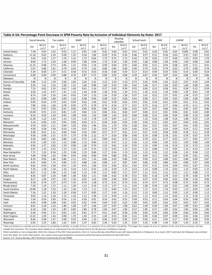
31

Table A-5A: Percentage Point Decrease in SPM Poverty Rate by Inclusion of Individual Elements by State: 2017 Social Security Tax credits SNAP SSI Housing

subsidies School lunch TANF LIHEAP WIC

Est M.O.E. (+/-)1 Est M.O.E

. (+/-)1 Est M.O.E. (+/-)1 Est M.O.E

. (+/-)1 Est M.O.E. (+/-)1 Est M.O.E

. (+/-)1 Est M.O.E. (+/-)1 Est M.O.E

. (+/-)1 Est M.O.E. (+/-)1

United States 7.38 0.04 1.92 0.03 1.21 0.03 1.09 0.02 0.66 0.02 0.41 0.01 0.20 0.01 0.05 0.005 0.08 0.01 Alabama 11.14 0.62 2.24 0.58 1.32 0.56 1.86 0.59 0.54 0.54 0.46 0.57 0.15 0.56 0.03 0.55 0.07 0.55 Alaska 3.03 1.65 1.27 1.76 1.41 1.72 0.66 1.73 0.75 1.72 0.26 1.70 0.63 1.75 0.06 1.70 0.03 1.70 Arizona 8.00 1.72 2.24 1.68 0.99 1.68 0.64 1.70 0.29 1.69 0.49 1.68 0.08 1.69 0.00 1.69 0.08 1.68 Arkansas 11.15 0.98 2.73 0.95 1.21 0.93 1.76 0.99 0.69 0.92 0.60 0.92 0.21 0.93 0.08 0.91 0.11 0.91 California 5.07 0.80 1.81 0.79 0.92 0.79 1.02 0.80 0.84 0.80 0.50 0.79 0.33 0.79 0.03 0.79 0.08 0.79 Colorado 5.34 0.60 1.37 0.51 0.58 0.55 0.63 0.56 0.46 0.54 0.17 0.53 0.09 0.54 0.02 0.54 0.00 0.54 Connecticut 6.89 0.90 0.99 0.88 0.76 0.87 0.75 0.89 0.93 0.88 0.29 0.87 0.30 0.87 0.03 0.86 0.01 0.86 Delaware N N N N N N N N N N N N N N N N N N District of Columbia 3.80 2.14 1.39 2.08 1.83 2.03 2.32 2.23 2.43 2.10 0.73 2.05 0.49 2.04 0.16 2.07 0.34 2.04 Florida 9.29 1.61 2.16 1.60 1.31 1.60 0.98 1.60 0.53 1.60 0.42 1.60 0.17 1.60 0.03 1.60 0.08 1.60 Georgia 7.23 0.61 2.55 0.62 1.40 0.61 1.16 0.57 0.45 0.59 0.55 0.60 0.12 0.58 0.01 0.58 0.13 0.59 Hawaii 6.03 1.42 0.57 1.41 1.16 1.44 0.36 1.38 0.50 1.39 0.15 1.39 0.23 1.39 0.00 1.39 0.02 1.39 Idaho 8.74 1.65 2.16 1.63 0.92 1.59 1.13 1.56 0.29 1.58 0.37 1.61 0.22 1.57 0.01 1.58 0.15 1.57 Illinois 6.92 0.98 1.89 0.99 1.56 0.98 0.96 0.98 0.59 0.98 0.44 0.98 0.17 0.99 0.05 0.98 0.08 0.98 Indiana 9.04 0.64 1.70 0.63 0.94 0.62 1.06 0.61 0.58 0.63 0.43 0.62 0.18 0.61 0.03 0.61 0.11 0.62 Iowa 7.80 0.81 1.60 0.78 0.95 0.75 0.79 0.74 0.26 0.77 0.27 0.75 0.16 0.77 0.06 0.76 0.11 0.76 Kansas 7.56 0.93 2.00 0.91 0.66 0.85 0.85 0.86 0.34 0.86 0.42 0.87 0.07 0.86 0.01 0.85 0.07 0.86 Kentucky 10.40 0.91 2.13 0.81 1.25 0.82 1.52 0.83 0.61 0.82 0.47 0.80 0.13 0.81 0.06 0.81 0.20 0.80 Louisiana 8.54 0.93 2.30 0.92 1.89 0.95 1.93 0.89 1.03 0.93 0.60 0.90 0.23 0.90 0.04 0.89 0.10 0.89 Maine 11.20 1.23 1.42 1.14 1.52 1.16 1.78 1.19 0.97 1.12 0.17 1.10 0.20 1.08 0.16 1.08 0.23 1.10 Maryland 5.24 0.96 1.42 0.95 0.96 0.94 0.71 0.94 0.60 0.95 0.30 0.94 0.13 0.95 0.07 0.94 0.03 0.95 Massachusetts 6.56 0.63 1.11 0.64 1.03 0.63 1.46 0.61 1.70 0.62 0.28 0.61 0.27 0.62 0.07 0.61 0.05 0.62 Michigan 9.50 0.58 1.94 0.54 1.59 0.55 1.33 0.55 0.70 0.54 0.40 0.54 0.19 0.54 0.09 0.54 0.12 0.54 Minnesota 6.48 0.61 1.21 0.60 0.66 0.56 0.83 0.57 0.77 0.61 0.15 0.57 0.24 0.58 0.06 0.58 0.11 0.58 Mississippi 9.36 0.90 2.31 0.79 1.75 0.78 2.12 0.77 0.50 0.80 0.60 0.76 0.08 0.78 0.01 0.79 0.07 0.79 Missouri 9.36 0.82 1.85 0.80 1.20 0.76 1.23 0.80 0.41 0.76 0.33 0.78 0.21 0.77 0.03 0.77 0.05 0.77 Montana 9.33 1.30 1.55 1.15 0.80 1.13 0.96 1.13 0.47 1.11 0.36 1.13 0.06 1.09 0.23 1.09 0.00 1.09 Nebraska 6.94 1.27 2.02 1.33 0.90 1.26 0.70 1.25 0.61 1.24 0.35 1.25 0.09 1.24 0.16 1.25 0.13 1.24 Nevada 6.47 1.15 2.23 1.14 1.35 1.10 0.74 1.13 0.35 1.13 0.41 1.15 0.08 1.14 0.05 1.13 0.10 1.14 New Hampshire 7.72 1.35 0.34 1.25 0.38 1.22 0.86 1.27 0.54 1.23 0.10 1.23 0.10 1.22 0.04 1.23 0.04 1.22 New Jersey 5.89 0.96 1.43 0.96 0.94 0.96 0.80 0.95 0.80 0.95 0.19 0.95 0.11 0.95 0.03 0.95 0.01 0.95 New Mexico 8.29 0.96 1.86 0.86 2.11 0.91 1.16 0.86 0.63 0.88 0.19 0.90 0.22 0.88 0.01 0.88 0.09 0.87 New York 6.45 0.86 1.75 0.85 1.55 0.86 1.26 0.86 1.27 0.87 0.40 0.86 0.30 0.86 0.05 0.86 0.07 0.86 North Carolina 8.62 0.56 2.38 0.55 1.34 0.55 1.06 0.52 0.40 0.53 0.42 0.53 0.15 0.53 0.04 0.53 0.07 0.52 North Dakota 5.32 1.18 1.24 1.16 0.24 1.13 0.22 1.16 0.29 1.13 0.14 1.14 0.08 1.14 0.02 1.14 0.03 1.15 Ohio 8.67 1.12 1.90 1.12 1.40 1.12 1.45 1.11 0.82 1.11 0.37 1.11 0.31 1.11 0.12 1.11 0.08 1.11 Oklahoma 8.56 0.87 2.29 0.80 1.48 0.82 1.51 0.84 0.62 0.78 0.51 0.81 0.18 0.79 0.03 0.79 0.06 0.79 Oregon 8.27 1.00 2.07 1.02 1.50 0.95 1.02 0.96 0.48 0.94 0.32 0.97 0.29 0.96 0.05 0.96 0.18 0.96 Pennsylvania 9.18 0.74 1.37 0.73 1.45 0.74 1.28 0.73 0.51 0.73 0.35 0.74 0.17 0.73 0.08 0.73 0.09 0.73 Rhode Island 7.30 1.19 1.72 1.11 1.29 1.11 2.19 1.13 1.57 1.11 0.34 1.08 0.39 1.05 0.02 1.09 0.03 1.08 South Carolina 10.00 1.18 2.35 1.16 1.36 1.14 1.11 1.13 0.64 1.14 0.52 1.13 0.13 1.14 0.03 1.13 0.03 1.14 South Dakota 7.14 1.21 1.20 1.26 0.58 1.17 0.85 1.17 0.34 1.16 0.12 1.13 0.06 1.12 0.03 1.13 0.09 1.12 Tennessee 9.03 1.16 2.18 1.15 1.35 1.12 1.28 1.12 0.43 1.12 0.44 1.12 0.22 1.12 0.03 1.12 0.16 1.12 Texas 5.56 0.56 2.83 0.56 1.33 0.56 0.91 0.54 0.42 0.55 0.58 0.55 0.11 0.54 0.04 0.54 0.08 0.55 Utah 4.69 0.68 2.08 0.65 0.65 0.62 0.45 0.64 0.20 0.62 0.38 0.63 0.05 0.62 0.02 0.62 0.07 0.62 Vermont 8.81 2.18 1.23 1.89 1.68 1.97 1.68 1.87 0.97 1.98 0.63 1.94 0.39 1.90 0.07 1.89 0.03 1.88 Virginia 6.18 1.85 1.33 1.85 0.83 1.86 0.78 1.85 0.47 1.85 0.27 1.85 0.17 1.85 0.02 1.85 0.06 1.85 Washington 6.44 0.64 1.41 0.63 1.05 0.61 0.77 0.61 0.64 0.58 0.38 0.60 0.20 0.60 0.04 0.60 0.04 0.60 West Virginia 13.22 1.09 1.56 0.98 1.79 1.03 2.35 1.04 0.53 0.92 0.21 0.94 0.40 0.97 0.09 0.92 0.06 0.93 Wisconsin 8.44 0.98 1.47 0.98 0.93 0.96 1.10 0.96 0.50 0.95 0.37 0.96 0.21 0.95 0.17 0.95 0.08 0.95 Wyoming 6.93 1.55 1.80 1.62 0.65 1.47 0.65 1.46 0.42 1.45 0.29 1.45 0.38 1.44 0.04 1.43 0.19 1.43 1Data are based on a sample and are subject to sampling variability. A margin of error is a measure of an estimate’s variability. The larger the margin of error in relation to the size of the estimate, the less reliable the estimate. This number when added to or subtracted from the estimate forms the 90 percent confidence interval. N Not available or not comparable. After the release of the 2017 data products, the U.S. Census Bureau identified issues with data collection in Delaware. As a result, 2017 estimates for Delaware are omitted from this table. For more information, see <www.census.gov/programs-surveys/acs/technical-documentation/errata/120.html>. Source: U.S. Census Bureau, 2017 American Community Survey PUMS.

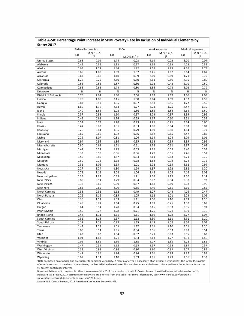
32

Table A-5B: Percentage Point Increase in SPM Poverty Rate by Inclusion of Individual Elements by State: 2017 Federal Income tax FICA Work expenses Medical expenses

Est M.O.E. (+/-)1 Est M.O.E. (+/-)1 Est M.O.E. (+/-

)1 Est M.O.E. (+/-)1

United States 0.68 0.02 1.74 0.03 2.19 0.03 3.70 0.04 Alabama 0.46 0.56 1.32 0.57 1.94 0.53 4.23 0.52 Alaska 0.65 1.77 1.44 1.72 1.59 1.73 2.56 1.75 Arizona 0.65 1.68 1.89 1.67 2.45 1.67 3.64 1.67 Arkansas 0.42 0.88 1.40 0.89 2.09 0.89 4.21 0.79 California 1.26 0.79 2.60 0.80 2.81 0.80 4.15 0.80 Colorado 0.56 0.53 1.57 0.50 2.03 0.48 3.10 0.50 Connecticut 0.86 0.83 1.74 0.80 1.86 0.78 3.02 0.79 Delaware N N N N N N N N District of Columbia 0.76 2.07 1.60 2.06 1.97 1.99 1.66 2.05 Florida 0.78 1.60 2.15 1.60 2.64 1.59 4.52 1.59 Georgia 0.62 0.57 1.95 0.57 2.53 0.56 4.22 0.55 Hawaii 1.60 1.36 2.64 1.27 2.74 1.25 4.47 1.19 Idaho 0.40 1.56 1.08 1.56 1.58 1.54 3.64 1.50 Illinois 0.57 0.98 1.60 0.97 2.03 0.97 3.39 0.96 Indiana 0.45 0.61 1.24 0.59 1.67 0.60 3.51 0.59 Iowa 0.51 0.73 1.28 0.73 1.75 0.71 3.34 0.66 Kansas 0.47 0.83 1.31 0.83 1.80 0.84 3.03 0.82 Kentucky 0.26 0.81 1.35 0.79 1.89 0.80 4.14 0.77 Louisiana 0.65 0.86 1.92 0.86 2.82 0.85 4.47 0.86 Maine 0.29 1.07 0.81 1.06 1.15 1.04 3.04 1.01 Maryland 0.94 0.95 1.86 0.95 2.18 0.95 3.39 0.96 Massachusetts 0.80 0.61 1.51 0.61 1.78 0.61 2.97 0.62 Michigan 0.42 0.54 1.29 0.53 1.85 0.53 3.40 0.53 Minnesota 0.33 0.58 0.96 0.56 1.29 0.55 2.46 0.57 Mississippi 0.40 0.80 1.47 0.84 2.11 0.83 4.71 0.75 Missouri 0.50 0.78 1.38 0.78 1.83 0.78 3.74 0.76 Montana 0.31 1.06 1.55 1.01 2.02 0.95 3.62 0.99 Nebraska 0.27 1.24 1.30 1.24 1.97 1.22 2.82 1.20 Nevada 0.73 1.12 2.08 1.06 2.48 1.08 4.16 1.08 New Hampshire 0.35 1.22 0.93 1.21 1.08 1.19 2.50 1.14 New Jersey 0.80 0.94 1.79 0.94 2.07 0.94 3.38 0.93 New Mexico 0.38 0.89 0.99 0.87 1.88 0.89 3.38 0.96 New York 0.88 0.85 2.00 0.85 2.40 0.85 3.66 0.85 North Carolina 0.53 0.51 1.62 0.49 2.27 0.48 4.16 0.47 North Dakota 0.22 1.16 0.85 1.05 1.12 1.01 2.23 1.02 Ohio 0.36 1.11 1.03 1.11 1.50 1.10 2.79 1.10 Oklahoma 0.45 0.77 1.64 0.75 1.99 0.75 4.30 0.69 Oregon 0.64 0.94 1.78 0.94 2.15 0.93 3.95 0.91 Pennsylvania 0.45 0.72 1.28 0.71 1.75 0.71 3.39 0.70 Rhode Island 0.44 1.11 1.31 1.11 1.89 1.08 3.27 1.07 South Carolina 0.51 1.13 1.57 1.12 2.30 1.11 3.91 1.10 South Dakota 0.19 1.13 0.79 1.13 1.43 1.02 3.07 1.04 Tennessee 0.44 1.12 1.55 1.12 2.05 1.10 4.11 1.10 Texas 0.60 0.54 1.95 0.54 2.56 0.53 3.87 0.54 Utah 0.43 0.62 1.54 0.62 2.21 0.63 3.55 0.62 Vermont 1.04 1.83 1.71 1.83 2.13 1.77 4.31 1.40 Virginia 0.96 1.85 1.86 1.85 2.07 1.85 3.73 1.85 Washington 0.47 0.59 1.32 0.58 1.57 0.58 2.84 0.57 West Virginia 0.33 0.91 0.94 0.90 1.80 0.85 3.77 0.84 Wisconsin 0.49 0.95 1.24 0.94 1.66 0.93 2.82 0.91 Wyoming 0.69 1.34 1.10 1.39 1.95 1.29 2.56 1.33 1Data are based on a sample and are subject to sampling variability. A margin of error is a measure of an estimate’s variability. The larger the margin of error in relation to the size of the estimate, the less reliable the estimate. This number when added to or subtracted from the estimate forms the 90 percent confidence interval. N Not available or not comparable. After the release of the 2017 data products, the U.S. Census Bureau identified issues with data collection in Delaware. As a result, 2017 estimates for Delaware are omitted from this table. For more information, see <www.census.gov/programs-surveys/acs/technical-documentation/errata/120.html>. Source: U.S. Census Bureau, 2017 American Community Survey PUMS.