the research supplemental poverty measure: 2012 research on the supplemental poverty measure (spm)...

U.S. Department of Commerce Economics and Statistics Administration U.S. CENSUS BUREAU census.gov

The Research SUPPLEMENTAL POVERTY MEASURE: 2012

Current Population Reports

By Kathleen ShortIssued November 2013P60-247

IntroductIon

This is the third report describ-ing research on the Supplemental Poverty Measure (SPM) released by the U.S. Census Bureau, with support from the Bureau of Labor Statistics (BLS).1 The SPM extends the official poverty measure by tak-ing account of many of the govern-ment programs designed to assist low-income families and individuals that are not included in the cur-rent official poverty measure. The current official poverty measure was developed in the early 1960s, and only a few minor changes have been implemented since it was first adopted in 1969 (Orshansky, 1963, 1965a, 1965b; Fisher, 1992). The official measure consists of a set of thresholds for families of different sizes and compositions that are compared with before-tax cash income to determine a fam-ily’s poverty status. At the time they were developed, the official poverty thresholds represented the cost of

1 Short (2011), <www.census.gov/hhes /povmeas/methodology/supplemental /research/Short_ResearchSPM2010.pdf> and Short (2012), <www.census.gov/hhes /povmeas/methodology/supplemental /research/Short_ResearchSPM2011.pdf>, accessed August 2013.

a minimum diet multiplied by three (to allow for expenditures on other goods and services).

Concerns about the adequacy of the official measure have increased during the past decades (Ruggles, 1990), culminating in a Congressional appropriation in 1990 for an independent scientific study of the concepts, measurement meth-ods, and information needed for a poverty measure. In response, the National Academy of Sciences (NAS) established the Panel on Poverty and Family Assistance, which released its report Measuring Poverty: A New Approach in the spring of 1995 (Citro and Michael, 1995). In March of 2010, the Interagency Technical Working Group on Developing a Supplemental Poverty Measure (ITWG) listed suggestions for research on the SPM. The ITWG was charged with developing a set of initial starting points to permit the Census Bureau, in cooperation with the BLS, to produce a report on the SPM that would be released along with the official measure each year. Their suggestions included:

• TheSPM thresholds should represent a dollar amount spent on a basic set of goods that

includes food, clothing, shelter, and utilities (FCSU) and a small additional amount to allow for other needs (e.g., household sup-plies, personal care, non-work-related transportation). This threshold should be calculated with five years of expenditure data for families with exactly two children using Consumer Expenditure Survey data, and it should be adjusted (using a spec-ified equivalence scale) to reflect the needs of different family types and geographic differences in housing costs. Adjustments to thresholds should be made over time to reflect real change in expenditures on this basic bundle of goods at the 33rd percentile of the expenditure distribution.

• SPM family resources should be defined as the value of cash income from all sources, plus the value of noncash benefits that are available to buy the basic bundle of goods (FCSU) minus necessary expenses for critical goods and services not included in the thresholds. Noncash ben-efits include nutrition assistance, subsidized housing, and home

2 U.S. Census Bureau

energy assistance. Necessary expenses that must be sub-tracted include income taxes, Social Security payroll taxes, childcare and other work-related expenses, child support pay-ments to another household, and contributions toward the cost of medical care and health insurance premiums, or medical out-of-pocket (MOOP) costs.2

This report presents a poverty measure that is based largely on the NAS panel’s 1995 recommen-dations and reflects more recent research and suggestions from the ITWG. Particular emphasis is on internal consistency between the thresholds and resources. The NAS panel noted: “It is important that family resources are defined consistently with the threshold concept in any poverty measure.”3 The SPM, as defined by the ITWG, is an internally consistent poverty measure that is based on spending “outflows” and money “inflows.” Spending outflows, or outlays, are those for basic needs only: FCSU and other basic necessary goods and services.4 Resources include money income from all sources plus the value of noncash benefits that help the family meet spending needs, less necessary expenses, like work-related expenses and taxes that must be paid. A family is designated as poor if its annual money inflow, net of necessary expenses, falls below its threshold level of money outflow.5

2 For information, see ITWG, Observations from the Interagency Technical Working Group on Developing a Supplemental Poverty Measure (Interagency), March 2010, available at <www.census.gov/hhes/www/poverty /SPM_TWGObservations.pdf>, accessed September 2013.

3 Citro and Michael, 1995, p. 9.4 For the BLS definition of expenditure

outlays, see Rogers and Gray, 1994.5 See Garner and Short, 2010, for further

discussion of measurement consistency.

The SPM does not take account of assets that may be used to meet necessary expenses. Since assets can add to the resources that are used to meet basic needs, some analysts advocate counting them in measuring poverty. Others may argue that many assets are not liquid or suggest that poor families have so few assets that including them would not change poverty measures much. If our purpose is to target families who are in need, then it is clear that families with no assets are worse off than those who have some. On the other hand, families who have incurred large debts are more vulnerable to finan-cial trouble than those who have not. The NAS panel discussed a “crisis definition of resources.” This definition included those assets families have on hand that could be converted to cash to support current consumption. They sug-gested that this “crisis definition” is only relevant for a very short-term measure of poverty because, in their words, “…assets can only ameliorate poverty temporarily.”6 They suggested that it is important, however, to develop measures of the distribution of wealth and to examine the relationship between asset ownership and poverty sta-tus. While spending down assets can enhance income to make ends meet, servicing debt can be a drain on family income that would other-wise be sufficient to purchase basic necessities.7

The ITWG stated that the official poverty measure, as defined in

6 Citro and Michael, 1995, pp. 214–218.7 Interest payments on mortgages are

included in SPM thresholds as a part of shel-ter costs, while income from assets, such as interest and dividends, are included in cash income. Short and Ruggles (2005) examined methods of taking account of net worth in experimental poverty measures using data from the Survey of Income and Program Participation (SIPP).

Office of Management and Budget (OMB) Statistical Policy Directive No. 14, will not be replaced by the SPM. They noted that the official measure is sometimes identified in legislation regarding program eligibility and funding distribution, while the SPM will not be used in this way. The SPM is designed to provide information on aggre-gate levels of economic need at a national level or within large subpopulations or areas and, as such, the SPM will be an additional macroeconomic statistic providing further understanding of economic conditions and trends.

This report presents updated esti-mates of the prevalence of poverty in the United States, overall and for selected demographic groups, using the official measure and the SPM. Section one presents differ-ences between the official poverty measure and the SPM. Comparing the two measures sheds light on the effects of noncash benefits, taxes, and other nondiscretionary expenses on measured economic wellbeing. The composition of the poverty populations using the two measures is examined across subgroups to better understand the incidence and receipt of benefits and taxes that are missed in the official statistics. The distribution of income-to-poverty threshold ratios and poverty rates by state are estimated and compared for the two measures. The second section of the report examines the SPM itself. Effects of benefits and expenses on SPM rates are explic-itly examined, and SPM estimates for 2012 are compared with the 2011 figures to assess changes in SPM rates from the previous year.

U.S. Census Bureau 3

Poverty estImates for 2012: offIcIal and sPm

The measures presented in this study use the 2013 Current Popu-lation Survey Annual Social and Economic Supplement (CPS ASEC) income information that refers to calendar year 2012 to estimate SPM resources.8 These are the same data used for the preparation of official poverty statistics and reported in DeNavas-Walt et al. (2013).

The “Orshansky” thresholds are used for the official poverty

8 The data in this report are from the 2011 to 2013 Current Population Survey Annual Social and Economic Supplement (CPS ASEC). The estimates in this paper (which may be shown in text, figures, and tables) are based on responses from a sample of the population and may differ from actual values because of sampling variability or other factors. As a result, apparent differences between the estimates for two or more groups may not be statistically significant. All comparative state-ments have undergone statistical testing and are significant at the 90 percent confidence level unless otherwise noted. Standard errors were calculated using replicate weights. Further information about the source and accuracy of the estimates is available at <www.census.gov/hhes/www/p60_239sa .pdf>, <www.census.gov/hhes/www /p60_243sa.pdf>, and <www.census.gov /hhes/www/p60_245sa.pdf>, accessed September 2013.

estimates presented here, how-ever, unlike the official estimates, unrelated individuals under the age of 15 are included in the universe. Since the CPS ASEC does not ask income questions for individuals under age 15, they are excluded from the universe for official pov-erty calculations. For the official poverty estimates shown in this report, all unrelated individuals under age 15 are included and presumed to be in poverty. For the SPM, they are assumed to share resources with the household refer-ence person.

The SPM thresholds for 2012 are based on out-of-pocket spend-ing on FCSU. Thresholds use five years of quarterly data from the Consumer Expenditure Survey (CE); the thresholds are produced by staff at the BLS.9, 10 Three housing status groups were determined and their expenditures on shelter

9 Bureau of Labor Statistics, Experimental Poverty Measure Web site, <www.bls.gov/pir /spmhome.htm>, accessed September 2013.

10 See <www.bls.gov/cex/anthology08 /csxanth2.pdf> or <www.bls.gov/cex /anthology08/csxanth3.pdf> for information on the CE, accessed September 2013.

and utilities produced within the 30–36th percentiles of FCSU expen-ditures.11 The three groups include owners with mortgages, owners without mortgages, and renters. The thresholds used here include the value of Supplemental Nutrition Assistance Program (SNAP) benefits in the measure of spending on food.12 The American Community Survey (ACS) data on rents paid are used to adjust the FCSU thresh-olds for differences in spending on housing across geographic areas.13

The two measures use different units of analysis. The official mea-sure of poverty uses the census-defined family that includes all indi-viduals residing together who are related by birth, marriage, or adop-tion and treats all unrelated individ-uals over age 15 independently. For the SPM, the ITWG suggested that

11 See appendix for description of threshold calculation.

12 For consistency in measurement with the resource measure, the thresholds should include the value of noncash benefits, though additional research continues at BLS on appropriate methods.

13 See appendix for description of the geographic adjustments.

Poverty measure concepts: official and supplemental

Official Poverty Measure Supplemental Poverty Measure

Measurement Units

Families and unrelated individuals

All related individuals who live at the same address, including any coresident unrelated children who are cared for by the family (such as foster children) and any cohabitors and their relatives

Poverty Threshold

Three times the cost of a minimum food diet in 1963

The 33rd percentile of expenditures on food, clothing, shelter, and utilities (FCSU) of consumer units with exactly two children multiplied by 1.2

Threshold Adjustments

Vary by family size, composition, and age of householder

Geographic adjustments for differences in housing costs by tenure and a three-parameter equivalence scale for family size and composition

Updating Thresholds

Consumer Price Index: all items

Five-year moving average of expenditures on FCSU

Resource Measure

Gross before-tax cash income

Sum of cash income, plus noncash benefits that families can use to meet their FCSU needs, minus taxes (or plus tax credits), minus work expenses, minus out-of-pocket medical expenses and child support paid to another household


the “family unit” should include all related individuals who live at the same address, as well as any coresident unrelated children who are cared for by the family (such as foster children), and any cohabitors and their children. Independent unrelated individuals living alone are one-person SPM units. This definition corresponds broadly with the unit of data collection (the consumer unit) that is employed for the CE data used to calculate poverty thresholds. These units are referred to as SPM Resource Units. Selection of the unit of analysis for poverty measurement implies that members of that unit share income or resources with one another.

SPM thresholds are adjusted for the size and composition of the SPM Resource Unit relative to the two-adult-two-child threshold using an equivalence scale.14 The official measure adjusts thresholds based on family size, number of children and adults, as well as whether or not the householder is aged 65 or over. The official poverty threshold for a two-adult-two-child family

14 See appendix for description of the three-parameter scale.

was $23,283 in 2012. The SPM thresholds vary by housing tenure status and are higher for owners with mortgages and renters than the official threshold. These two groups comprise about 76 percent of the total population. The offi-cial threshold increased by $472 between 2011 and 2012. SPM thresholds for owners increased significantly between 2011 and 2012, but the increase was less than the increase in the official threshold for the same period. The SPM thresholds for renters declined between the two years.

Following the recommendations of the NAS report and the ITWG, SPM resources are estimated as the sum of cash income; plus any federal government noncash benefits

that families can use to meet their FCSU needs; minus taxes (plus tax credits), work expenses, and out-of-pocket expenditures for medical expenses. The research SPM pre-sented in this study adds the value of noncash benefits and subtracts necessary expenses, such as taxes, child care expenses, and MOOP expenses. For the SPM, estimates from additional questions about child care and medical out-of-pocket expenses are available and subtracted from income.15 The text box summarizes the additions and subtractions for the SPM; descrip-tions are in the appendix.

15 Documentation concerning the quality of these data is available in various working papers at <www.census.gov/hhes/povmeas /publications/working.html>, accessed September 2013.

two adult, two child Poverty thresholds: 2011 and 2012(Dollars)

2011 S.E. 2012 S.E.

Official . . . . . . . . . . . . . . . . . . . . . . . . . . . . . . . . . . 22,811 X 23,283 X

Research Supplemental Poverty MeasureOwners with a mortgage . . . . . . . . . . . . . . . . . . 25,703 347 25,784 368Owners without a mortgage . . . . . . . . . . . . . . . . 21,175 298 21,400 233

Renters . . . . . . . . . . . . . . . . . . . . . . . . . . . . . . . 25,222 378 25,105 398

S.E. Standard error. X Not applicable.Source: Bureau of Labor Statistics, September 2013 <www.bls.gov/pir/spmhome.htm>.

resource estimatessPm resources = money Income from all sources

Plus: Minus:

Supplemental Nutritional Assistance (SNAP)

National School Lunch Program

Supplementary Nutrition Program for Women, Infants, and Children (WIC)

Housing Subsidies

Low-Income Home Energy Assistance (LIHEAP)

Taxes (plus credits such as the Earned Income Tax Credit [EITC])

Expenses Related to Work

Child Care Expenses

Medical Out-of-Pocket (MOOP) Expenses

Child Support Paid


Poverty rates: offIcIal and sPm

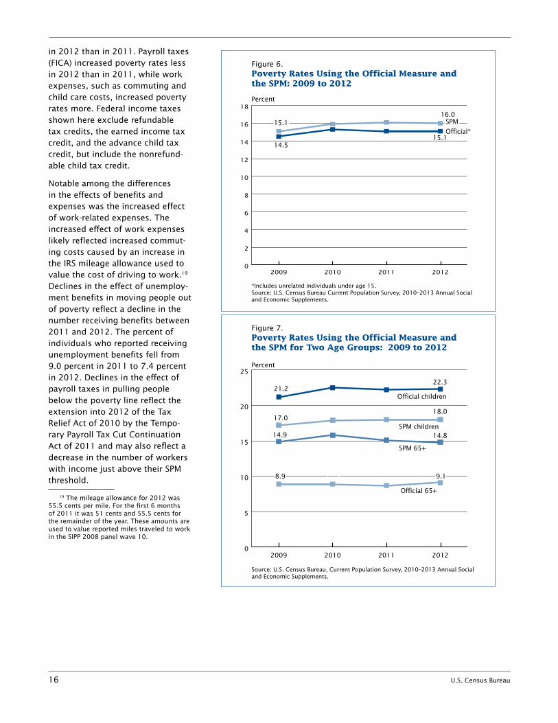
Figure 1 shows poverty rates for the two measures for the total pop-ulation and for three age groups: under 18 years, ages 18 to 64, and 65 years and over. Table 1 shows rates for a variety of selected demographic groups. The percent of the population that was poor using the official measure for 2012 was 15.0 percent (DeNavas-Walt et al., 2013). For this study, including unrelated individuals under age 15 in the universe, the poverty rate was 15.1 percent.16 The research SPM yields a rate of 16.0 percent for 2012. While, as noted, SPM poverty thresholds are generally higher than official thresholds, other parts of the measure also contribute to differences in the estimated prevalence of poverty in the United States.

In 2012, 49.7 million were poor using the SPM definition of poverty, more than the 47.0 million using the official definition of poverty with our universe. For most groups, SPM rates were higher than the offi-cial poverty rates. Comparing the SPM to the official measure shows lower poverty rates for children, individuals included in new SPM Resource Units, Blacks, renters, those living outside metropolitan areas, those in the Midwest, those covered by only public health insur-ance, and individuals with a work disability. Most other groups had higher poverty rates using the SPM rather than the official measure. Official and SPM poverty rates for females, people in female house-holder units, native-born citizens, residents of the South, and those not working were not statistically different. Note that poverty rates

16 The 15.0 and 15.1 rates are not statisti-cally different.

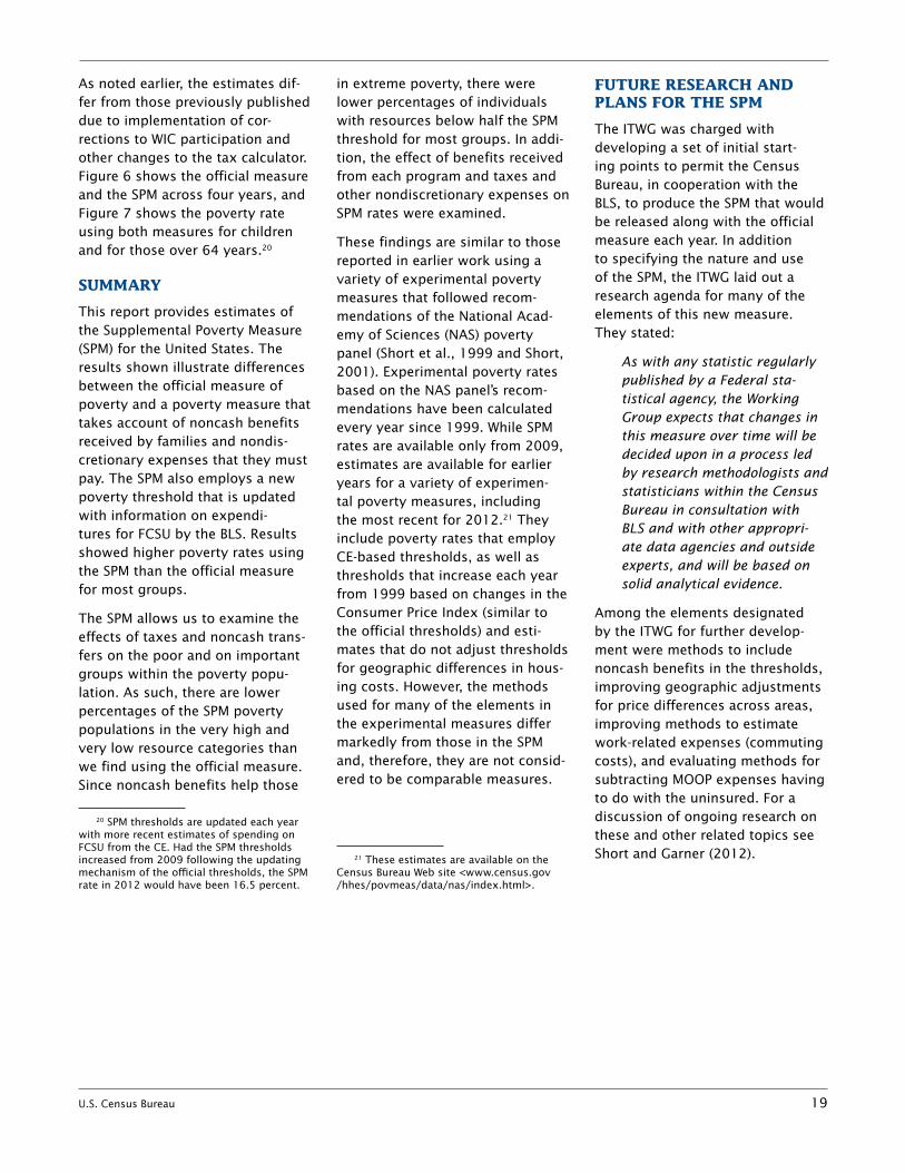
for those 65 years and over were higher under the SPM compared with the official measure. This partially reflects that the official thresholds are set lower for fami-lies with householders in this age group, while the SPM thresholds do not vary by age.

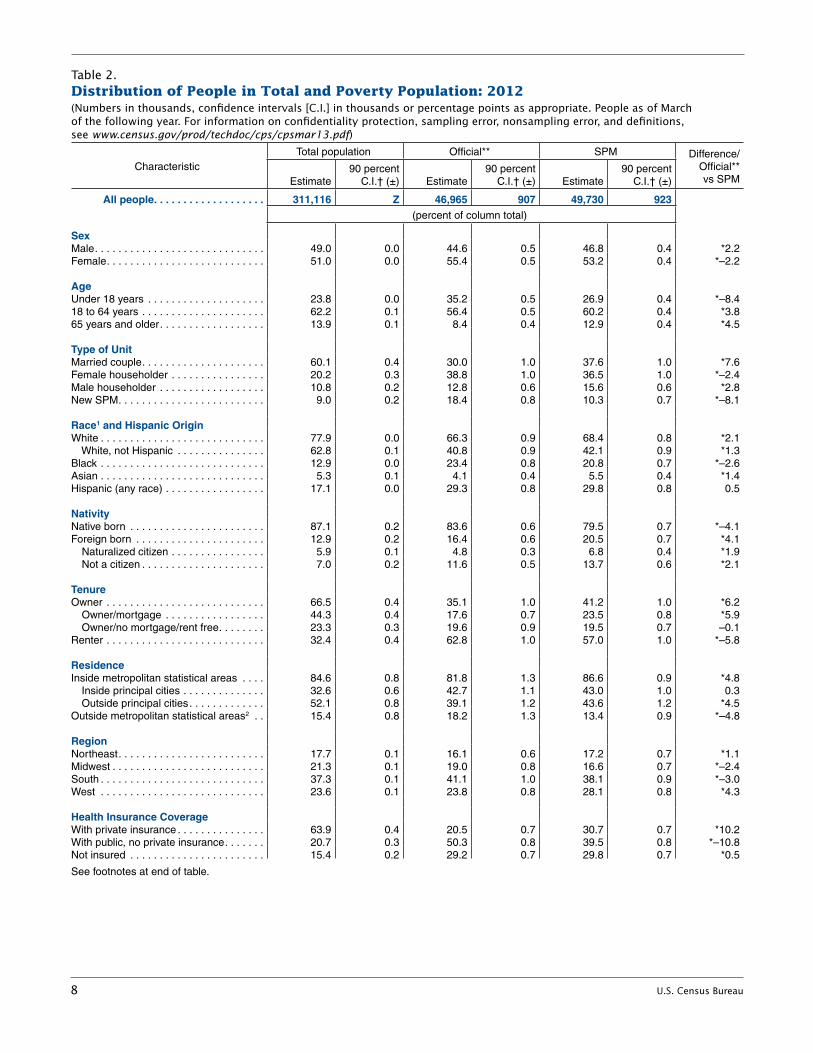
dIstrIbutIon of the Poverty PoPulatIon by characterIstIcs: offIcIal and sPm

Table 2 compares the distribution of people in the total population across selected groups with the distribution of people classified as poor using the two measures. Fig-ure 2 shows these estimates across age groups. The top bar shows the representation of these groups in the total population. The share of people 65 years and over in pov-erty was higher when the SPM is

used, 12.9 percent compared with 8.4 percent with the official mea-sure, while the share of children was lower.

The SPM also results in a higher share of the poor for men, those who were 18 to 64 years old, in married-couple families, with male householders, Whites, Asians, the foreign born, homeowners with mortgages, individuals with private health insurance, the uninsured, all workers, and individuals without a work disability. The shares were also higher using the SPM rather than the official measure for those residing in metropolitan areas but outside principal cities and the Northeast and West regions. These differences by residence and region reflect the adjustments for geographic cost differences in housing that are made to the SPM thresholds.

Figure 1.Poverty Rates Using Two Measures for Total Population by Age Group: 2012

0

5

10

15

20

25

65 years and older

18 to 64 years

Under 18 years

All people

*Includes unrelated individuals under the age of 15.Source: U.S. Census Bureau, Current Population Survey, 2013 Annual Social and Economic Supplement.

Official*SPMPercent


Table 1. number and Percentage of People in Poverty by different Poverty measures: 2012(Numbers in thousands, confidence intervals [C.I.] in thousands or percentage points as appropriate. People as of March of the following year. For information on confidentiality protection, sampling error, nonsampling error, and definitions, see www.census.gov/prod/techdoc/cps/cpsmar13.pdf)

Characteristic

Number**(in thousands)

Official** SPMDifference

Number Percent Number Percent

Esti-mate

90 percent C.I.† (±)

Esti-mate

90 percent

C.I.† (±)

Esti-mate

90 percent

C.I.† (±)

Esti-mate

90 percent

C.I.† (±) Number Percent

All people . . . . . . . . . . . . . .

Sex

311,116 46,965 907 15 .1 0 .3 49,730 923 16 .0 0 .3 *2,766 *0 .9

Male . . . . . . . . . . . . . . . . . . . . . . . . 152,335 20,934 471 13.7 0.3 23,278 474 15.3 0.3 *2,345 *1.5Female . . . . . . . . . . . . . . . . . . . . . .

Age

158,781 26,031 531 16.4 0.3 26,452 534 16.7 0.3 421 0.3

Under 18 years . . . . . . . . . . . . . . . 74,187 16,542 451 22.3 0.6 13,358 366 18.0 0.5 *–3,184 *–4.318 to 64 years . . . . . . . . . . . . . . . . 193,642 26,497 522 13.7 0.3 29,953 584 15.5 0.3 *3,456 *1.865 years and older . . . . . . . . . . . . .

Type of Unit

43,287 3,926 174 9.1 0.4 6,419 217 14.8 0.5 *2,493 *5.8

Married couple . . . . . . . . . . . . . . . . 186,869 14,081 577 7.5 0.3 18,703 668 10.0 0.4 *4,622 *2.5Female householder . . . . . . . . . . . 62,778 18,244 597 29.1 0.8 18,137 577 28.9 0.8 –108 –0.2Male householder . . . . . . . . . . . . . 33,554 6,015 277 17.9 0.7 7,766 291 23.1 0.7 *1,751 *5.2New SPM . . . . . . . . . . . . . . . . . . . .

Race1 and Hispanic Origin

27,914 8,625 381 30.9 1.0 5,124 360 18.4 1.1 *–3,501 *–12.5

White . . . . . . . . . . . . . . . . . . . . . . . 242,469 31,139 714 12.8 0.3 34,002 724 14.0 0.3 *2,864 *1.2White, not Hispanic . . . . . . . . . . 195,330 19,158 598 9.8 0.3 20,946 596 10.7 0.3 *1,788 *0.9

Black . . . . . . . . . . . . . . . . . . . . . . . 40,208 10,994 424 27.3 1.1 10,363 415 25.8 1.0 *–631 *–1.6Asian . . . . . . . . . . . . . . . . . . . . . . . 16,433 1,937 190 11.8 1.1 2,737 213 16.7 1.2 *800 *4.9Hispanic (any race) . . . . . . . . . . . .

Nativity

53,230 13,740 456 25.8 0.9 14,819 450 27.8 0.8 *1,078 *2.0

Native born . . . . . . . . . . . . . . . . . . 271,010 39,243 834 14.5 0.3 39,538 837 14.6 0.3 295 0.1Foreign born . . . . . . . . . . . . . . . . . 40,107 7,721 305 19.3 0.6 10,192 367 25.4 0.7 *2,471 *6.2

Naturalized citizen . . . . . . . . . . . 18,200 2,260 158 12.4 0.8 3,361 195 18.5 0.9 *1,101 *6.1Not a citizen . . . . . . . . . . . . . . . .

Tenure

21,906 5,462 256 24.9 1.0 6,831 307 31.2 1.1 *1,369 *6.2

Owner . . . . . . . . . . . . . . . . . . . . . . 206,922 16,469 591 8.0 0.3 20,512 604 9.9 0.3 *4,043 *2.0 Owner/mortgage . . . . . . . . . . . . 137,771 8,254 384 6.0 0.3 11,676 443 8.5 0.3 *3,422 *2.5

Owner/no mortgage/rent free . . . 72,546 9,201 447 12.7 0.5 9,694 402 13.4 0.5 *493 *0.7Renter . . . . . . . . . . . . . . . . . . . . . .

ResidenceInside metropolitan statistical

100,799 29,509 735 29.3 0.6 28,360 747 28.1 0.7 *–1,148 *–1.1

areas . . . . . . . . . . . . . . . . . . . . . . . 263,328 38,411 918 14.6 0.3 43,064 956 16.4 0.3 *4,653 *1.8Inside principal cities . . . . . . . . . 101,363 20,071 614 19.8 0.5 21,401 667 21.1 0.6 *1,329 *1.3Outside principal cities . . . . . . . .

Outside metropolitan statistical 161,965 18,340 669 11.3 0.4 21,664 701 13.4 0.4 *3,324 *2.1

areas2 . . . . . . . . . . . . . . . . . . . . . .

Region

47,788 8,553 644 17.9 0.9 6,666 478 13.9 0.7 *–1,887 *–3.9

Northeast . . . . . . . . . . . . . . . . . . . . 55,135 7,575 304 13.7 0.6 8,570 362 15.5 0.7 *996 *1.8Midwest . . . . . . . . . . . . . . . . . . . . . 66,422 8,936 390 13.5 0.6 8,268 382 12.4 0.6 *–668 *–1.0South . . . . . . . . . . . . . . . . . . . . . . . 116,130 19,279 690 16.6 0.6 18,939 605 16.3 0.5 –340 –0.3West . . . . . . . . . . . . . . . . . . . . . . .

Health Insurance Coverage

73,429 11,175 409 15.2 0.6 13,953 473 19.0 0.6 *2,778 *3.8

With private insurance . . . . . . . . . .With public, no private

198,812 9,615 386 4.8 0.2 15,273 446 7.7 0.2 *5,658 *2.8

insurance . . . . . . . . . . . . . . . . . . . 64,354 23,614 613 36.7 0.7 19,655 559 30.5 0.7 *–3,959 *–6.2Not insured . . . . . . . . . . . . . . . . . .

See footnotes at end of table.

47,951 13,735 408 28.6 0.7 14,802 449 30.9 0.8 *1,067 *2.2


The share of the poor who were in the category labeled “new SPM units” was lower than the offi-cial measure by 8.1 percentage points—these are the units that include additional members, such as cohabiting partners, whose income is not included in the family definition employed by the official measure. The proportion that were female, children, resided in female-householder families, Blacks, native born, renters, living outside metropolitan areas, in the Midwest and the South, had only public insurance, did not work, and had a work disability was smaller using the SPM compared with the official measure. The shares of the poverty

Table 1. number and Percentage of People in Poverty by different Poverty measures: 2012—Con.(Numbers in thousands, confidence intervals [C.I.] in thousands or percentage points as appropriate. People as of March of the following year. For information on confidentiality protection, sampling error, nonsampling error, and definitions, see www.census.gov/prod/techdoc/cps/cpsmar13.pdf)

Characteristic

Number** (in thousands)

Official** SPMDifference


Esti-mate

90 percent

C.I.† (±)

Esti-mate

90 percent

C.I.† (±)

Esti-mate

90 percent

C.I.† (±)

Esti-mate

90 percent

C.I.† (±) Number Percent

Work Experience Total, 18 to 64 years . . . . . . . 193,642 26,497 522 13.7 0.3 29,953 584 15.5 0.3 *3,456 *1.8All workers . . . . . . . . . . . . . . . . . . . . 145,814 10,672 294 7.3 0.2 14,066 358 9.6 0.2 *3,394 *2.3 Worked full-time, year-round . . . . 98,715 2,867 133 2.9 0.1 5,252 183 5.3 0.2 *2,385 *2.4 Less than full-time, year-round . . 47,099 7,805 233 16.6 0.5 8,814 275 18.7 0.5 *1,009 *2.1Did not work at least 1 week . . . . . . 47,828 15,825 369 33.1 0.6 15,887 390 33.2 0.7 62 0.1

Disability Status3

Total, 18 to 64 years . . . . . . . 193,642 26,497 522 13.7 0.3 29,953 584 15.5 0.3 *3,456 *1.8With a disability . . . . . . . . . . . . . . . . 14,996 4,257 161 28.4 0.9 3,979 167 26.5 0.9 *–278 *–1.9With no disability . . . . . . . . . . . . . . . 177,727 22,189 478 12.5 0.3 25,921 536 14.6 0.3 *3,732 *2.1

* Statistically different from zero at the 90 percent confidence level.** Includes unrelated individuals under the age of 15.† A 90 percent confidence interval is a measure of an estimate’s variability. The larger the confidence interval in relation to the size of the estimate, the less

reliable the estimate. Confidence intervals shown in this table are based on standard errors calculated using replicate weights. For more information see “Standard Errors and Their Use” at <www.census.gov/hhes/www/p60_245sa.pdf>.

1 Federal surveys give respondents the option of reporting more than one race. Therefore, two basic ways of defining a race group are possible. A group such as Asian may be defined as those who reported Asian and no other race (the race-alone or single-race concept) or as those who reported Asian regardless of whether they also reported another race (the race-alone-or-in-combination concept). This table shows data using the first approach (race alone). The use of the single-race population does not imply that it is the preferred method of presenting or analyzing data. The Census Bureau uses a variety of approaches. Information on people who reported more than one race, such as White and American Indian and Alaska Native or Asian and Black or African American, is available from Census 2010 through American FactFinder. About 2.9 percent of people reported more than one race in Census 2010. Data for American Indians and Alaska Natives, Native Hawaiians and Other Pacific Islanders, and those reporting two or more races are not shown separately.

2 The “Outside metropolitan statistical areas” category includes both micropolitan statistical areas and territory outside of metropolitan and micropolitan statisti-cal areas. For more information, see “About Metropolitan and Micropolitan Statistical Areas” at <www.census.gov/population/metro>.

3 The sum of those with and without a disability does not equal the total because disability status is not defined for individuals in the Armed Forces.Source: U.S. Census Bureau, Current Population Survey, 2013 Annual Social and Economic Supplement.

SPM

Official*

Total

Figure 2.Composition of Total and Poverty Populations by Age Group: 2012

*Includes unrelated individuals under the age of 15.Source: U.S. Census Bureau, Current Population Survey, 2013 Annual Social and Economic Supplement.

Under 18 years

35.2

23.8 13.9

26.9 60.2

56.4

62.2

8.4

12.9

(In percent)

65 years and older18 to 64 years


Table 2.distribution of People in total and Poverty Population: 2012(Numbers in thousands, confidence intervals [C.I.] in thousands or percentage points as appropriate. People as of March of the following year. For information on confidentiality protection, sampling error, nonsampling error, and definitions, see www.census.gov/prod/techdoc/cps/cpsmar13.pdf)

CharacteristicTotal population Official** SPM Difference/

Official** vs SPMEstimate

90 percent C.I.† (±) Estimate



All people . . . . . . . . . . . . . . . . . . .

Sex

311,116 Z 46,965 907 49,730 923 (percent of column total)

Male . . . . . . . . . . . . . . . . . . . . . . . . . . . . . 49.0 0.0 44.6 0.5 46.8 0.4 *2.2Female . . . . . . . . . . . . . . . . . . . . . . . . . . .

Age

51.0 0.0 55.4 0.5 53.2 0.4 *–2.2

Under 18 years . . . . . . . . . . . . . . . . . . . . 23.8 0.0 35.2 0.5 26.9 0.4 *–8.418 to 64 years . . . . . . . . . . . . . . . . . . . . . 62.2 0.1 56.4 0.5 60.2 0.4 *3.865 years and older . . . . . . . . . . . . . . . . . .

Type of Unit

13.9 0.1 8.4 0.4 12.9 0.4 *4.5

Married couple . . . . . . . . . . . . . . . . . . . . . 60.1 0.4 30.0 1.0 37.6 1.0 *7.6Female householder . . . . . . . . . . . . . . . . 20.2 0.3 38.8 1.0 36.5 1.0 *–2.4Male householder . . . . . . . . . . . . . . . . . . 10.8 0.2 12.8 0.6 15.6 0.6 *2.8New SPM . . . . . . . . . . . . . . . . . . . . . . . . .


9.0 0.2 18.4 0.8 10.3 0.7 *–8.1

White . . . . . . . . . . . . . . . . . . . . . . . . . . . . 77.9 0.0 66.3 0.9 68.4 0.8 *2.1White, not Hispanic . . . . . . . . . . . . . . . 62.8 0.1 40.8 0.9 42.1 0.9 *1.3

Black . . . . . . . . . . . . . . . . . . . . . . . . . . . . 12.9 0.0 23.4 0.8 20.8 0.7 *–2.6Asian . . . . . . . . . . . . . . . . . . . . . . . . . . . . 5.3 0.1 4.1 0.4 5.5 0.4 *1.4Hispanic (any race) . . . . . . . . . . . . . . . . .

Nativity

17.1 0.0 29.3 0.8 29.8 0.8 0.5

Native born . . . . . . . . . . . . . . . . . . . . . . . 87.1 0.2 83.6 0.6 79.5 0.7 *–4.1Foreign born . . . . . . . . . . . . . . . . . . . . . . 12.9 0.2 16.4 0.6 20.5 0.7 *4.1

Naturalized citizen . . . . . . . . . . . . . . . . 5.9 0.1 4.8 0.3 6.8 0.4 *1.9Not a citizen . . . . . . . . . . . . . . . . . . . . .

Tenure

7.0 0.2 11.6 0.5 13.7 0.6 *2.1

Owner . . . . . . . . . . . . . . . . . . . . . . . . . . . 66.5 0.4 35.1 1.0 41.2 1.0 *6.2 Owner/mortgage . . . . . . . . . . . . . . . . . 44.3 0.4 17.6 0.7 23.5 0.8 *5.9

Owner/no mortgage/rent free . . . . . . . . 23.3 0.3 19.6 0.9 19.5 0.7 –0.1Renter . . . . . . . . . . . . . . . . . . . . . . . . . . .

Residence

32.4 0.4 62.8 1.0 57.0 1.0 *–5.8

Inside metropolitan statistical areas . . . . 84.6 0.8 81.8 1.3 86.6 0.9 *4.8Inside principal cities . . . . . . . . . . . . . . 32.6 0.6 42.7 1.1 43.0 1.0 0.3Outside principal cities . . . . . . . . . . . . . 52.1 0.8 39.1 1.2 43.6 1.2 *4.5

Outside metropolitan statistical areas2 . .

Region

15.4 0.8 18.2 1.3 13.4 0.9 *–4.8

Northeast . . . . . . . . . . . . . . . . . . . . . . . . . 17.7 0.1 16.1 0.6 17.2 0.7 *1.1Midwest . . . . . . . . . . . . . . . . . . . . . . . . . . 21.3 0.1 19.0 0.8 16.6 0.7 *–2.4South . . . . . . . . . . . . . . . . . . . . . . . . . . . . 37.3 0.1 41.1 1.0 38.1 0.9 *–3.0West . . . . . . . . . . . . . . . . . . . . . . . . . . . .


23.6 0.1 23.8 0.8 28.1 0.8 *4.3

With private insurance . . . . . . . . . . . . . . . 63.9 0.4 20.5 0.7 30.7 0.7 *10.2With public, no private insurance . . . . . . . 20.7 0.3 50.3 0.8 39.5 0.8 *–10.8Not insured . . . . . . . . . . . . . . . . . . . . . . . 15.4 0.2 29.2 0.7 29.8 0.7 *0.5



population of Hispanics, those who owned their home without a mort-gage, or resided inside principal cities were not statistically different under the two measures.

distribution of Income-to-Poverty threshold ratios: official and sPm

Comparing the distribution of gross cash income with that of SPM resources also allows an exami-nation of the effect of taxes and transfers on SPM rates. Table 3 shows the distribution of income-to-poverty threshold ratios for various groups. Dividing income by the respective poverty threshold controls income by unit size and composition. Figure 3 shows the

percent distribution of income-to-threshold ratio categories for all people.

In general, the comparison sug-gests that a smaller percentage of the population was in the lowest category of the distribution using the SPM. For most groups, includ-ing targeted noncash benefits reduced the percentage of the population in the lowest category—those with income below half their poverty threshold. This was true for most of the groups shown in Table 3 except for those over age 64. They showed a higher percent below half of the poverty line with the SPM: 4.7 percent compared to 2.7 percent with the official

measure. As shown earlier, many of the noncash benefits included in the SPM are not targeted to this population. Further, many trans-fers received by this group are in cash, especially Social Security payments, and are captured in the official measure as well as the SPM. Note that the percentage of the 65 years and over age group with cash income below half their threshold was lower than that of other age groups under the official measure (2.7 percent), while the percent-age for children was higher (10.3 percent). Subtracting MOOP and other expenses and adding non-cash benefits in the SPM narrowed the differences across the three age groups.

Table 2.distribution of People in total and Poverty Population: 2012—Con.(Numbers in thousands, confidence intervals [C.I.] in thousands or percentage points as appropriate. People as of March of the following year. For information on confidentiality protection, sampling error, nonsampling error, and definitions, see www.census.gov/prod/techdoc/cps/cpsmar13.pdf)

CharacteristicTotal population Official** SPM Difference/

Official** vs SPMEstimate




Work Experience Total, 18 to 64 years . . . . . . . . . . .All workers . . . . . . . . . . . . . . . . . . . . . . . . Worked full-time, year-round . . . . . . . . Less than full-time, year-round . . . . . .Did not work at least 1 week . . . . . . . . . .

Disability Status3

Total, 18 to 64 years . . . . . . . . . . .With a disability . . . . . . . . . . . . . . . . . . . .With no disability . . . . . . . . . . . . . . . . . . .

(percent of column total)

*3.8*5.6*4.5*1.1

*–1.7

*3.8*–1.1*4.9

62.246.931.715.115.4

62.24.8

57.1

0.10.20.20.20.2

0.10.10.1

56.422.76.1

16.633.7

56.49.1

47.2

0.50.50.20.40.5

0.50.30.5

60.228.310.617.731.9

60.28.0

52.1

0.40.50.30.40.5

0.40.30.5

Z Rounds to zero.* Statistically different from zero at the 90 percent confidence level.** Includes unrelated individuals under the age of 15. † A 90 percent confidence interval is a measure of an estimate’s variability. The larger the confidence interval in relation to the size of the estimate, the less




3 The sum of those with and without a disability does not equal the total because disability status is not defined for individuals in the Armed Forces.Source: U.S. Census Bureau, Current Population Survey, 2013 Annual Social and Economic Supplement.


On the other hand, the SPM shows a smaller percentage with income or resources in the high-est category—four or more times the thresholds. The SPM resource measure subtracts taxes, compared with the official measure that does not, bringing down the percent-age of people with income in the highest category.

Table 3 shows similar calcula-tions by race and ethnicity. Using the SPM, smaller percentages had income below half of their pov-erty thresholds, compared with the official measure, for all groups shown except for Asians. The per-centage of Asians in this category was not statistically different with the two measures. For Blacks, the

percentage in this lowest category was 12.8 percent with the official measure and 7.7 percent with the SPM. The percentage of Whites and Hispanics in the lowest category was also lower using the SPM.

Another notable difference between the distributions using these two measures was the larger number

Table 3.Percentage of People by ratio of Income/resources to Poverty threshold: 2012(Numbers in thousands, confidence intervals [C.I.] in thousands or percentage points as appropriate. People as of March of the following year. For information on confidentiality protection, sampling error, nonsampling error, and definitions, see www.census.gov/prod/techdoc/cps/cpsmar13.pdf)

Characteristic

Less than 0.5 0.5 to 0.99 1.0 to 1.49 1.5 to 1.99 2.0 to 3.99 4.0 or more

Esti-mate


Esti-mate


Esti-mate


Esti-mate


Esti-mate


Esti-mate


OFFICIAL**

All people . . . . . . . . . . . .

Age

6 .7 0 .2 8 .4 0 .2 9 .6 0 .2 9 .6 0 .2 30 .0 0 .4 35 .7 0 .4

Under 18 years . . . . . . . . 10.3 0.4 12.0 0.5 11.5 0.4 10.4 0.4 29.0 0.5 26.9 0.518 to 64 years . . . . . . . . . 6.2 0.2 7.4 0.2 8.5 0.2 8.6 0.2 29.5 0.4 39.7 0.465 years and older . . . . . .


2.7 0.2 6.4 0.4 11.8 0.5 12.8 0.6 33.7 0.8 32.6 0.7

White . . . . . . . . . . . . . . . . 5.5 0.2 7.3 0.2 9.2 0.2 9.5 0.2 30.4 0.4 38.1 0.5 White, not Hispanic . . . . 4.4 0.2 5.4 0.2 7.6 0.2 8.5 0.3 30.8 0.5 43.3 0.5Black . . . . . . . . . . . . . . . . 12.8 0.8 14.5 0.7 12.4 0.7 10.8 0.7 29.3 1.0 20.2 0.8Asian . . . . . . . . . . . . . . . . 5.8 0.7 6.0 0.9 7.5 1.0 8.3 0.9 27.4 1.4 45.0 1.8Hispanic (any race) . . . . .

SPM

10.3 0.5 15.5 0.7 15.7 0.8 13.2 0.6 28.5 0.8 16.7 0.7

All people . . . . . . . . . . . .

Age

5 .2 0 .2 10 .8 0 .3 17 .0 0 .3 14 .2 0 .3 34 .6 0 .4 18 .2 0 .3

Under 18 years . . . . . . . . 4.7 0.2 13.3 0.4 21.4 0.5 16.3 0.5 32.7 0.6 11.7 0.418 to 64 years . . . . . . . . . 5.4 0.2 10.1 0.3 15.1 0.3 13.4 0.3 35.7 0.4 20.3 0.365 years and older . . . . . .


4.7 0.3 10.1 0.4 18.0 0.6 14.3 0.6 33.1 0.8 19.7 0.7

White . . . . . . . . . . . . . . . . 4.6 0.2 9.4 0.3 15.9 0.3 13.9 0.3 36.0 0.4 20.2 0.3 White, not Hispanic . . . . 4.0 0.2 6.7 0.3 13.0 0.3 13.4 0.3 39.2 0.4 23.7 0.4Black . . . . . . . . . . . . . . . . 7.7 0.6 18.0 0.9 23.0 1.0 16.4 0.8 27.0 1.0 7.9 0.5Asian . . . . . . . . . . . . . . . . 6.0 0.7 10.6 1.1 15.5 1.3 13.6 1.1 35.7 1.7 18.6 1.2Hispanic (any race) . . . . . 7.2 0.5 20.6 0.8 27.8 0.9 15.7 0.7 22.8 0.8 5.8 0.3

** Includes unrelated individuals under the age of 15.† A 90 percent confidence interval is a measure of an estimate’s variability. The larger the confidence interval in relation to the size of the estimate, the

less reliable the estimate. Confidence intervals shown in this table are based on standard errors calculated using replicate weights. For more information, see “Standard Errors and Their Use” at <www.census.gov/hhes/www/p60_245sa.pdf>.

1 Federal surveys give respondents the option of reporting more than one race. Therefore, two basic ways of defining a race group are possible. A group such as Asian may be defined as those who reported Asian and no other race (the race-alone or single-race concept) or as those who reported Asian regard-less of whether they also reported another race (the race-alone-or-in-combination concept). This table shows data using the first approach (race alone). The use of the single-race population does not imply that it is the preferred method of presenting or analyzing data. The Census Bureau uses a variety of approaches. Information on people who reported more than one race, such as White and American Indian and Alaska Native or Asian and Black or African American, is available from Census 2010 through American FactFinder. About 2.9 percent of people reported more than one race in Census 2010. Data for American Indians and Alaska Natives, Native Hawaiians and Other Pacific Islanders, and those reporting two or more races are not shown separately.

Source: U.S. Census Bureau, Current Population Survey, 2013 Annual Social and Economic Supplement.


of individuals with income-to-threshold ratios in the three middle categories with the SPM. Since the effect of taxes and transfers is often to move family income from the extremes of the distribu-tion to the center of the distribu-tion, that is, from the very bottom with targeted transfers or from the very top via taxes and other expenses, the increase in the size of these middle categories is to be expected. One group of interest is that just above the respective pov-erty thresholds, with resources or income between 1.0 and 1.5 times their threshold. This group was 9.6 percent of the population using the official measure and 17.0 percent of the population using the SPM.17 Altogether, about 53 million people were not poor but fell in this low-

17 Renwick and Short (2013) show that the group below 1.4 times the SPM threshold are similar to the number of individuals with resources below family budgets adjusted to be comparable to the SPM. They use budgets developed by the Economic Policy Institute for 2008 for these comparisons.

income category. Combined with those below the poverty threshold, about 103 million people lived below 1.5 times the SPM threshold.

Poverty rates by state: official and sPm

The Census Bureau recommends using the American Community Survey (ACS) for state-level pov-erty estimates. However, the SPM cannot be calculated using data from that survey. With the CPS, the Census Bureau recommends the use of 3-year averages to compare estimates across states. Table 4 shows 3-year averages of poverty rates for the two measures for the U.S. total and for each state. The 3-year average poverty rates for the United States for the years 2010, 2011, and 2012 were 15.1 percent with the official measure and 16.0 percent using the SPM.

Figure 4 shows the United States divided into three categories by

state: states with higher and lower rates using the SPM compared with the official measure and states that are not statistically different. The 13 states for which the SPM rates were higher than the official poverty rates are those with lighter shades. These states were Califor-nia, Colorado, Connecticut, Florida, Hawaii, Illinois, Maryland, Massa-chusetts, Nevada, New Hampshire, New Jersey, New York, and Virginia. The SPM rate for the District of Columbia was also higher. Higher SPM rates by state may occur from many sources. Geographic adjust-ments for housing costs may result in higher SPM thresholds, as well as a different mix of housing tenure or metropolitan area status, or higher nondiscretionary expenses, such as taxes or medical expenses.

Medium shades represent the 28 states where SPM rates were lower than the official poverty rates. These states were Alabama, Arkansas, Idaho, Indiana, Iowa, Kansas, Kentucky, Louisiana, Maine, Michigan, Minnesota, Mississippi, Missouri, Montana, Nebraska, New Mexico, North Carolina, North Dakota, Ohio, Oklahoma, South Carolina, South Dakota, Tennessee, Texas, Vermont, West Virginia, Wisconsin, and Wyoming. Lower SPM rates would occur due to lower thresholds reflecting lower housing costs, a different mix of housing tenure or metropolitan area status, or more generous noncash ben-efits. Darker shades are those nine states that were not statistically dif-ferent under the two measures and include Alaska, Arizona, Delaware, Georgia, Oregon, Pennsylvania, Rhode Island, Utah, and Washington State. Details are in Table 4.

Figure 3.Distribution of People by Income-to-Threshold Ratios: 2012

*Includes unrelated individuals under the age of 15. Note: Total does not sum to 100.0 due to rounding.Source: U.S. Census Bureau, Current Population Survey, 2013 Annual Social and Economic Supplement.

(In percent)

SPMOfficial*

30.0

9.6

9.6

35.718.2

34.6

17.0

14.2

10.88.4

6.7 5.2

4.0 or more

2.0 to 3.99

1.5 to 1.99

1.0 to 1.49

0.5 to 1.0

Less than 0.5


the suPPlemental Poverty measure

the effect of cash and noncash transfers, taxes, and other nondiscretionary expenses

The purpose of this section is to move away from comparing the SPM with the official measure and look only at changes within the SPM. This exercise allows us to gauge the effects of taxes and transfers and other necessary expenses using the SPM alone as the measure of economic well-being. The previous section char-acterized the poverty population using the SPM in comparison with the current official measure. This section examines that SPM poverty population in more detail.

The official poverty measure takes account of cash benefits from the government, such as Social Security and Unemployment Insurance (UI) benefits, Supplemental Security Income (SSI), public assistance ben-efits, such as Temporary Assistance for Needy Families (TANF), and workers compensation benefits, but does not take account of taxes or noncash benefits aimed at improving the economic situation of the poor. Besides taking account of cash benefits and necessary expenses, such as MOOP expenses and expenses related to work, the SPM includes taxes and noncash transfers. The important contribu-tion that the SPM provides is allow-ing us to gauge the effectiveness of tax credits and transfers in alleviat-ing poverty. We can also examine

the effects of the nondiscretionary expenses such as work expenses and MOOP.

Table 5a shows the effect that vari-ous additions and subtractions had on the SPM rate in 2012, holding all else the same and assuming no behavioral changes. Additions and subtractions are shown for the total population and by three age groups. Additions shown in the table include cash benefits, also accounted for in the official mea-sure, as well as noncash benefits, included only in the SPM. This allows us to examine the effects of government transfers on poverty estimates. Because child support paid is subtracted from income in the SPM, we also examine the effect of child support received on alleviating poverty. Child support

Figure 4.Difference in Poverty Rates by State Using the Official Measure and the SPM: 3-Year Average, 2010–2012

Source: U.S. Census Bureau, Current Population Survey, 2011–2013 Annual Social and Economic Supplements.

MT

AK

NM

OR MN

KS

SD

ND

MO

WA

FL

IL IN

WI NY

PA

MI

OH

IA

ME

MA

CT

AZ

NV

TX

COCA

WY

UT

ID

NE

OK

GA

AR

AL

NC

MS

LA

TN

KY

VA

SC

WV

RI

DE MD

NJ

HI

VTNH

DC *

Not statistically differentSPM lower than officialSPM higher than official


Table 4.number and Percentage of People in Poverty by state using 3-year averages over 2010,1 2011,1 and 2012(Numbers in thousands, confidence intervals [C.I.] in thousands or percentage points as appropriate. People as of March of the following year. For information on confidentiality protection, sampling error, nonsampling error, and definitions, see www.census.gov/prod/techdoc /cps/cpsmar13.pdf)

State

Official**3-year average

2010–2012

SPM3-year average

2010–2012Difference

Number


Percent-age

90 percent C.I.† (±) Number


Percent-age

90 percent C.I.† (±) Number Percent

United States . . . . . . . . . . . . . . . . . 46,783 597 15 .1 0 .2 49,380 619 16 .0 0 .2 *2,597 *0 .8

Alabama . . . . . . . . . . . . . . . . . . . . . . . 776 94 16.3 2.0 645 72 13.5 1.5 *–132 *–2.8Alaska . . . . . . . . . . . . . . . . . . . . . . . . . 82 11 11.6 1.5 88 10 12.5 1.4 6 0.9Arizona . . . . . . . . . . . . . . . . . . . . . . . . 1,208 141 18.5 2.2 1,231 135 18.8 2.1 22 0.3Arkansas . . . . . . . . . . . . . . . . . . . . . . . 525 60 18.1 2.1 479 46 16.5 1.6 *–46 *–1.6California . . . . . . . . . . . . . . . . . . . . . . . 6,202 230 16.5 0.6 8,952 290 23.8 0.8 *2,750 *7.3Colorado . . . . . . . . . . . . . . . . . . . . . . . 638 76 12.6 1.5 695 60 13.7 1.2 *57 *1.1Connecticut . . . . . . . . . . . . . . . . . . . . . 345 36 9.8 1.0 440 36 12.5 1.0 *95 *2.7Delaware . . . . . . . . . . . . . . . . . . . . . . . 119 11 13.2 1.2 124 11 13.9 1.2 6 0.6District of Columbia . . . . . . . . . . . . . . . 119 9 19.3 1.5 141 10 22.7 1.5 *21 *3.4Florida . . . . . . . . . . . . . . . . . . . . . . . . . 2,938 144 15.5 0.8 3,709 166 19.5 0.9 *771 *4.1

Georgia . . . . . . . . . . . . . . . . . . . . . . . . 1,789 126 18.5 1.3 1,760 137 18.2 1.4 –29 –0.3Hawaii . . . . . . . . . . . . . . . . . . . . . . . . . 173 22 12.9 1.7 231 24 17.3 1.8 *58 *4.4Idaho . . . . . . . . . . . . . . . . . . . . . . . . . . 232 30 14.8 2.0 183 24 11.6 1.6 *–49 *–3.1Illinois . . . . . . . . . . . . . . . . . . . . . . . . . . 1,748 117 13.7 0.9 1,943 113 15.2 0.9 *195 *1.5Indiana . . . . . . . . . . . . . . . . . . . . . . . . . 1,008 104 15.8 1.6 903 91 14.2 1.4 *–106 *–1.7Iowa . . . . . . . . . . . . . . . . . . . . . . . . . . . 316 29 10.5 0.9 258 21 8.6 0.7 *–59 *–1.9Kansas . . . . . . . . . . . . . . . . . . . . . . . . . 406 48 14.5 1.8 323 47 11.5 1.8 *–82 *–2.9Kentucky . . . . . . . . . . . . . . . . . . . . . . . 751 82 17.4 1.9 586 68 13.6 1.6 *–165 *–3.8Louisiana . . . . . . . . . . . . . . . . . . . . . . . 951 105 21.3 2.4 823 70 18.5 1.6 *–128 *–2.9Maine . . . . . . . . . . . . . . . . . . . . . . . . . . 173 17 13.1 1.3 148 15 11.2 1.2 *–25 *–1.9

Maryland . . . . . . . . . . . . . . . . . . . . . . . 588 50 10.1 0.9 783 64 13.4 1.1 *195 *3.3Massachusetts . . . . . . . . . . . . . . . . . . . 724 75 11.1 1.2 903 75 13.8 1.2 *180 *2.7Michigan . . . . . . . . . . . . . . . . . . . . . . . 1,449 114 14.9 1.2 1,318 112 13.5 1.2 *–130 *–1.3Minnesota . . . . . . . . . . . . . . . . . . . . . . 547 56 10.4 1.1 514 50 9.7 1.0 *–33 *–0.6Mississippi . . . . . . . . . . . . . . . . . . . . . . 606 55 20.7 1.9 471 40 16.1 1.4 *–135 *–4.6Missouri . . . . . . . . . . . . . . . . . . . . . . . . 910 122 15.3 2.1 738 112 12.4 1.9 *–172 *–2.9Montana . . . . . . . . . . . . . . . . . . . . . . . . 148 20 14.9 2.1 119 14 12.1 1.5 *–28 *–2.9Nebraska . . . . . . . . . . . . . . . . . . . . . . . 201 30 11.0 1.6 178 20 9.8 1.1 *–22 *–1.2Nevada . . . . . . . . . . . . . . . . . . . . . . . . 434 40 16.0 1.5 537 45 19.8 1.7 *102 *3.8New Hampshire . . . . . . . . . . . . . . . . . . 98 11 7.6 0.9 133 13 10.2 1.0 *34 *2.6

New Jersey . . . . . . . . . . . . . . . . . . . . . 930 98 10.7 1.1 1,345 118 15.5 1.3 *415 *4.8New Mexico.. . . . . . . . . . . . . . . . . . . . . 416 39 20.3 1.9 331 35 16.1 1.7 *–86 *–4.2New York . . . . . . . . . . . . . . . . . . . . . . . 3,179 164 16.5 0.9 3,487 155 18.1 0.8 *308 *1.6North Carolina . . . . . . . . . . . . . . . . . . . 1,596 149 16.8 1.6 1,348 130 14.2 1.4 *–249 *–2.6North Dakota . . . . . . . . . . . . . . . . . . . . 77 8 11.5 1.2 62 7 9.2 1.0 *–15 *–2.3Ohio . . . . . . . . . . . . . . . . . . . . . . . . . . . 1,748 171 15.4 1.5 1,496 118 13.2 1.0 *–252 *–2.2Oklahoma . . . . . . . . . . . . . . . . . . . . . . 606 55 16.3 1.5 501 49 13.4 1.3 *–105 *–2.8Oregon . . . . . . . . . . . . . . . . . . . . . . . . . 548 55 14.3 1.4 533 58 13.9 1.5 –14 –0.4Pennsylvania . . . . . . . . . . . . . . . . . . . . 1,652 121 13.1 1.0 1,596 105 12.6 0.8 –56 –0.4Rhode Island . . . . . . . . . . . . . . . . . . . . 143 14 13.8 1.3 141 11 13.6 1.1 –2 –0.2

South Carolina . . . . . . . . . . . . . . . . . . . 814 65 17.6 1.4 732 58 15.8 1.3 *–82 *–1.8South Dakota . . . . . . . . . . . . . . . . . . . . 113 17 13.9 2.2 86 11 10.6 1.4 *–27 *–3.3Tennessee . . . . . . . . . . . . . . . . . . . . . . 1,101 135 17.3 2.2 985 111 15.5 1.8 *–116 *–1.8Texas . . . . . . . . . . . . . . . . . . . . . . . . . . 4,549 253 17.7 1.0 4,211 237 16.4 0.9 *–338 *–1.3Utah . . . . . . . . . . . . . . . . . . . . . . . . . . . 302 40 10.7 1.4 326 56 11.6 2.0 23 0.8Vermont . . . . . . . . . . . . . . . . . . . . . . . . 70 7 11.3 1.2 62 7 10.1 1.2 *–8 *–1.3Virginia . . . . . . . . . . . . . . . . . . . . . . . . . 874 88 11.0 1.1 1,055 98 13.3 1.2 *181 *2.3Washington . . . . . . . . . . . . . . . . . . . . . 822 81 12.1 1.2 828 75 12.2 1.1 6 0.1West Virginia . . . . . . . . . . . . . . . . . . . . 313 43 17.2 2.3 235 30 12.9 1.6 *–78 *–4.3Wisconsin . . . . . . . . . . . . . . . . . . . . . . 664 70 11.7 1.2 611 71 10.8 1.3 *–53 *–0.9Wyoming . . . . . . . . . . . . . . . . . . . . . . . 58 8 10.2 1.3 52 7 9.2 1.2 *–6 *–1.0

* Statistically different from zero at the 90 percent confidence level.** Includes unrelated individuals under the age of 15.† A 90 percent confidence interval is a measure of an estimate’s variability. The larger the confidence interval in relation to the size of the estimate, the less reliable the

estimate. Confidence intervals shown in this table are based on standard errors calculated using replicate weights. For more information, see “Standard Errors and Their Use” at <www.census.gov/hhes/www/p60_245sa.pdf>.

1 Consistent with 2011 and 2012 data through implementation of Census 2010 based population controls. Figures differ from previously published estimates due to changes in the tax calculations and the valuation of WIC benefits. See Macartney, 2013.



payments received are counted as income in both the official measure and the SPM.

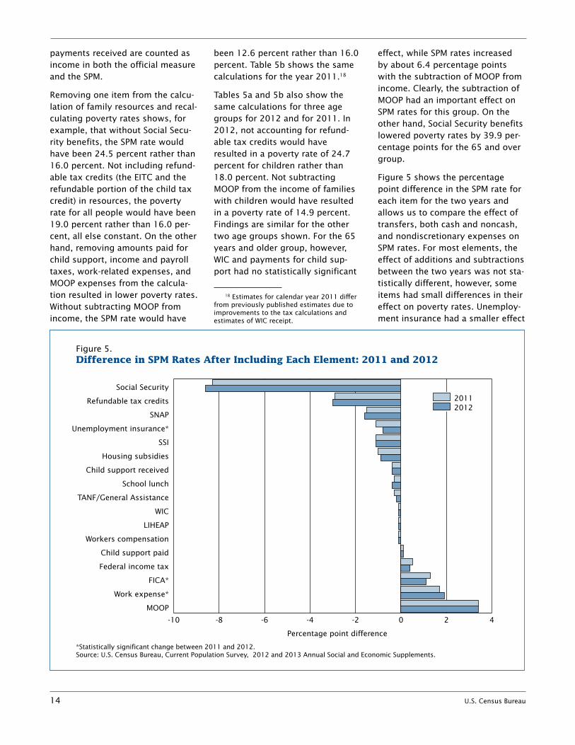
Removing one item from the calcu-lation of family resources and recal-culating poverty rates shows, for example, that without Social Secu-rity benefits, the SPM rate would have been 24.5 percent rather than 16.0 percent. Not including refund-able tax credits (the EITC and the refundable portion of the child tax credit) in resources, the poverty rate for all people would have been 19.0 percent rather than 16.0 per-cent, all else constant. On the other hand, removing amounts paid for child support, income and payroll taxes, work-related expenses, and MOOP expenses from the calcula-tion resulted in lower poverty rates. Without subtracting MOOP from income, the SPM rate would have

been 12.6 percent rather than 16.0 percent. Table 5b shows the same calculations for the year 2011.18

Tables 5a and 5b also show the same calculations for three age groups for 2012 and for 2011. In 2012, not accounting for refund-able tax credits would have resulted in a poverty rate of 24.7 percent for children rather than 18.0 percent. Not subtracting MOOP from the income of families with children would have resulted in a poverty rate of 14.9 percent. Findings are similar for the other two age groups shown. For the 65 years and older group, however, WIC and payments for child sup-port had no statistically significant

18 Estimates for calendar year 2011 differ from previously published estimates due to improvements to the tax calculations and estimates of WIC receipt.

effect, while SPM rates increased by about 6.4 percentage points with the subtraction of MOOP from income. Clearly, the subtraction of MOOP had an important effect on SPM rates for this group. On the other hand, Social Security benefits lowered poverty rates by 39.9 per-centage points for the 65 and over group.

Figure 5 shows the percentage point difference in the SPM rate for each item for the two years and allows us to compare the effect of transfers, both cash and noncash, and nondiscretionary expenses on SPM rates. For most elements, the effect of additions and subtractions between the two years was not sta-tistically different, however, some items had small differences in their effect on poverty rates. Unemploy-ment insurance had a smaller effect

Figure 5.Difference in SPM Rates After Including Each Element: 2011 and 2012

*Statistically significant change between 2011 and 2012.Source: U.S. Census Bureau, Current Population Survey, 2012 and 2013 Annual Social and Economic Supplements.

Percentage point difference

-10 -8 -6 -4 -2 0 2 4

MOOP

Work expense*

FICA*

Federal income tax

Child support paid

Workers compensation

LIHEAP

WIC

TANF/General Assistance

School lunch

Child support received

Housing subsidies

SSI

Unemployment insurance*

SNAP

Refundable tax credits

Social Security20112012


Table 5a.effect of excluding Individual elements on sPm rates: 2012(Confidence intervals [C.I.] in percentage points. Percent of people as of March of the following year. For information on confiden-tiality protection, sampling error, nonsampling error, and definitions, see www.census.gov/prod/techdoc/cps/cpsmar13.pdf)

ElementsAll persons Children Nonelderly adults 65 years and older

Estimate90 percent

C.I.† (±) Estimate90 percent



C.I.† (±)

Research SPM . . . . . . . . . . . . . . . . . . 16 .0 0 .3 18 .0 0 .5 15 .5 0 .3 14 .8 0 .5Social Security . . . . . . . . . . . . . . . . . . . 24.5 0.3 20.0 0.5 19.6 0.3 54.7 0.7Refundable tax credits . . . . . . . . . . . . . 19.0 0.3 24.7 0.6 17.7 0.3 15.0 0.5SNAP . . . . . . . . . . . . . . . . . . . . . . . . . . 17.6 0.3 21.0 0.5 16.7 0.3 15.6 0.5Unemployment insurance . . . . . . . . . . 16.8 0.3 18.8 0.5 16.4 0.3 15.1 0.5SSI . . . . . . . . . . . . . . . . . . . . . . . . . . . . 17.1 0.3 18.9 0.5 16.6 0.3 16.0 0.5Housing subsidies . . . . . . . . . . . . . . . . 16.9 0.3 19.4 0.5 16.1 0.3 16.0 0.5Child support received . . . . . . . . . . . . . 16.4 0.3 19.0 0.5 15.8 0.3 14.9 0.5School lunch . . . . . . . . . . . . . . . . . . . . 16.4 0.3 18.9 0.5 15.7 0.3 14.9 0.5TANF/General Assistance . . . . . . . . . . 16.2 0.3 18.5 0.5 15.6 0.3 14.9 0.5WIC . . . . . . . . . . . . . . . . . . . . . . . . . . . 16.1 0.3 18.3 0.5 15.6 0.3 14.8 0.5LIHEAP . . . . . . . . . . . . . . . . . . . . . . . . 16.1 0.3 18.1 0.5 15.5 0.3 14.9 0.5Workers compensation . . . . . . . . . . . . 16.1 0.3 18.1 0.5 15.6 0.3 14.9 0.5Child support paid . . . . . . . . . . . . . . . . 15.9 0.3 17.8 0.5 15.3 0.3 14.8 0.5Federal income tax . . . . . . . . . . . . . . . 15.6 0.3 17.7 0.5 14.9 0.3 14.6 0.5FICA . . . . . . . . . . . . . . . . . . . . . . . . . . 14.8 0.3 16.4 0.5 14.3 0.3 14.6 0.5Work expense . . . . . . . . . . . . . . . . . . . 14.1 0.3 15.4 0.5 13.5 0.3 14.4 0.5MOOP . . . . . . . . . . . . . . . . . . . . . . . . . 12.6 0.3 14.9 0.5 12.6 0.3 8.4 0.4

† A 90 percent confidence interval is a measure of an estimate’s variability. The larger the confidence interval in relation to the size of the estimate, the less reliable the estimate. Confidence intervals shown in this table are based on standard errors calculated using replicate weights. For more information see “Standard Errors and Their Use” at <www.census.gov/hhes/www/p60_245sa.pdf>.


Table 5b.effect of excluding Individual elements on sPm rates: 20111

(Confidence intervals [C.I.] in percentage points. Percent of people as of March of the following year. For information on confidentiality protection, sampling error, nonsampling error, and definitions, see www.census.gov/prod/techdoc/cps/cpsmar12.pdf)

All persons Children Nonelderly adults 65 years and olderElements 90 percent 90 percent 90 percent 90 percent

Estimate C.I.† (±) Estimate C.I.† (±) Estimate C.I.† (±) Estimate C.I.† (±)

Research SPM . . . . . . . . . . . . . . . . . . 16 .1 0 .3 18 .0 0 .5 15 .5 0 .3 15 .1 0 .5Social Security . . . . . . . . . . . . . . . . . . . 24.4 0.3 20.1 0.5 19.6 0.3 54.1 0.8Refundable tax credits . . . . . . . . . . . . . 18.9 0.3 24.3 0.6 17.6 0.3 15.2 0.5SNAP . . . . . . . . . . . . . . . . . . . . . . . . . . 17.6 0.3 20.9 0.5 16.7 0.3 15.8 0.6Unemployment insurance . . . . . . . . . . 17.2 0.3 19.3 0.5 16.7 0.3 15.5 0.5SSI . . . . . . . . . . . . . . . . . . . . . . . . . . . . 17.1 0.3 18.8 0.5 16.7 0.3 16.3 0.6Housing subsidies . . . . . . . . . . . . . . . . 17.0 0.3 19.4 0.5 16.2 0.3 16.3 0.6Child support received . . . . . . . . . . . . . 16.5 0.3 19.0 0.5 15.8 0.3 15.1 0.5School lunch . . . . . . . . . . . . . . . . . . . . 16.4 0.3 18.9 0.5 15.7 0.3 15.1 0.5TANF/General Assistance . . . . . . . . . . 16.3 0.3 18.6 0.5 15.7 0.3 15.1 0.5WIC . . . . . . . . . . . . . . . . . . . . . . . . . . . 16.2 0.3 18.4 0.5 15.6 0.3 15.1 0.5LIHEAP . . . . . . . . . . . . . . . . . . . . . . . . 16.1 0.3 18.1 0.5 15.6 0.3 15.1 0.5Workers compensation . . . . . . . . . . . . 16.2 0.3 18.1 0.5 15.6 0.3 15.1 0.5Child support paid . . . . . . . . . . . . . . . . 15.9 0.3 17.9 0.5 15.4 0.3 15.0 0.5Federal income tax . . . . . . . . . . . . . . . 15.6 0.3 17.7 0.5 14.9 0.3 14.8 0.5FICA . . . . . . . . . . . . . . . . . . . . . . . . . . 14.8 0.3 16.3 0.5 14.2 0.3 14.8 0.5Work expense . . . . . . . . . . . . . . . . . . . 14.4 0.3 15.7 0.5 13.8 0.3 14.7 0.5MOOP . . . . . . . . . . . . . . . . . . . . . . . . . 12.7 0.3 15.2 0.5 12.7 0.3 8.0 0.4

† A 90 percent confidence interval is a measure of an estimate’s variability. The larger the confidence interval in relation to the size of the estimate, the less reliable the estimate. Confidence intervals shown in this table are based on standard errors calculated using replicate weights. For more information see “Standard Errors and Their Use” at <www.census.gov/hhes/www/p60_243sa.pdf>.

1 Estimates for calendar year 2011 differ from previously published estimates due to changes to the tax calculations and the valuation of WIC benefits. See Macartney, 2013.



in 2012 than in 2011. Payroll taxes (FICA) increased poverty rates less in 2012 than in 2011, while work expenses, such as commuting and child care costs, increased poverty rates more. Federal income taxes shown here exclude refundable tax credits, the earned income tax credit, and the advance child tax credit, but include the nonrefund-able child tax credit.

Notable among the differences in the effects of benefits and expenses was the increased effect of work-related expenses. The increased effect of work expenses likely reflected increased commut-ing costs caused by an increase in the IRS mileage allowance used to value the cost of driving to work.19 Declines in the effect of unemploy-ment benefits in moving people out of poverty reflect a decline in the number receiving benefits between 2011 and 2012. The percent of individuals who reported receiving unemployment benefits fell from 9.0 percent in 2011 to 7.4 percent in 2012. Declines in the effect of payroll taxes in pulling people below the poverty line reflect the extension into 2012 of the Tax Relief Act of 2010 by the Tempo-rary Payroll Tax Cut Continuation Act of 2011 and may also reflect a decrease in the number of workers with income just above their SPM threshold.

19 The mileage allowance for 2012 was 55.5 cents per mile. For the first 6 months of 2011 it was 51 cents and 55.5 cents for the remainder of the year. These amounts are used to value reported miles traveled to work in the SIPP 2008 panel wave 10.

Figure 6.Poverty Rates Using the Official Measure and the SPM: 2009 to 2012

0

2

4

6

8

10

12

14

16

18

2012201120102009

*Includes unrelated individuals under age 15.Source: U.S. Census Bureau Current Population Survey, 2010–2013 Annual Social and Economic Supplements.

14.515.1

16.0

Percent

SPM

Official*15.1

Figure 7.Poverty Rates Using the Official Measure and the SPM for Two Age Groups: 2009 to 2012

0

5

10

15

20

25

2012201120102009


Official 65+

SPM children

SPM 65+

Official children21.2

18.0

22.3

14.8

17.0

14.9

Percent

8.9 9.1


Table 6.Percentage of People in Poverty using the supplemental Poverty measure: 2011 and 2012(Numbers in thousands. Confidence intervals [C.I.] in thousands or percentage points as appropriate. People as of March of the following year. For information on confidentiality protection, sampling error, nonsampling error, and definitions, see www.census.gov/prod/techdoc/cps/cpsmar13.pdf)

Characteristic

Below poverty level

DifferenceSPM 2012 SPM 20111


Estimate





All people . . . . . . . . . . . . . . . . . . . . . . . .

Sex

49,730 923 16 .0 0 .3 49,567 902 16 .1 0 .3 163 –0 .1

Male . . . . . . . . . . . . . . . . . . . . . . . . . . . . . 23,278 474 15.3 0.3 23,057 473 15.3 0.3 222 0.0Female . . . . . . . . . . . . . . . . . . . . . . . . . . .

Age

26,452 534 16.7 0.3 26,511 502 16.8 0.3 –59 –0.2

Under 18 years . . . . . . . . . . . . . . . . . . . . 13,358 366 18.0 0.5 13,349 376 18.0 0.5 9 0.018 to 64 years . . . . . . . . . . . . . . . . . . . . . 29,953 584 15.5 0.3 29,971 578 15.5 0.3 –18 0.065 years and older . . . . . . . . . . . . . . . . . .

Type of Unit

6,419 217 14.8 0.5 6,247 229 15.1 0.5 172 –0.2

Married couple . . . . . . . . . . . . . . . . . . . . . 18,703 668 10.0 0.4 18,488 631 9.9 0.3 215 0.1Female householder . . . . . . . . . . . . . . . . 18,137 577 28.9 0.8 18,969 516 29.9 0.7 *–832 *–1.1Male householder . . . . . . . . . . . . . . . . . . 7,766 291 23.1 0.7 7,071 313 21.9 0.9 *695 *1.3New SPM . . . . . . . . . . . . . . . . . . . . . . . . .


5,124 360 18.4 1.1 5,039 305 18.7 1.0 85 –0.4

White . . . . . . . . . . . . . . . . . . . . . . . . . . . . 34,002 724 14.0 0.3 34,339 732 14.2 0.3 –337 –0.2 White, not Hispanic . . . . . . . . . . . . . . . 20,946 596 10.7 0.3 21,406 586 11.0 0.3 –460 –0.2Black . . . . . . . . . . . . . . . . . . . . . . . . . . . . 10,363 415 25.8 1.0 10,180 405 25.6 1.0 182 0.1Asian . . . . . . . . . . . . . . . . . . . . . . . . . . . . 2,737 213 16.7 1.2 2,715 215 16.9 1.3 21 –0.2Hispanic (any race) . . . . . . . . . . . . . . . . .

Nativity

14,819 450 27.8 0.8 14,589 502 27.9 1.0 229 0.0

Native born . . . . . . . . . . . . . . . . . . . . . . . 39,538 837 14.6 0.3 39,280 754 14.6 0.3 258 0.0Foreign born . . . . . . . . . . . . . . . . . . . . . . 10,192 367 25.4 0.7 10,288 387 25.7 0.9 –96 –0.3 Naturalized citizen . . . . . . . . . . . . . . . . 3,361 195 18.5 0.9 3,280 184 18.3 0.9 81 0.2 Not a citizen . . . . . . . . . . . . . . . . . . . . .

Tenure

6,831 307 31.2 1.1 7,007 330 31.8 1.3 –176 –0.6

Owner . . . . . . . . . . . . . . . . . . . . . . . . . . . 20,512 604 9.9 0.3 19,955 615 9.7 0.3 557 0.3 Owner/mortgage . . . . . . . . . . . . . . . . . 11,676 443 8.5 0.3 11,114 479 8.1 0.3 561 0.3 Owner/no mortgage/rent free . . . . . . . . 9,694 402 13.4 0.5 9,580 397 13.0 0.5 114 0.3Renter . . . . . . . . . . . . . . . . . . . . . . . . . . .

ResidenceInside metropolitan statistical

28,360 747 28.1 0.7 28,873 735 29.3 0.6 –513 *–1.1

areas . . . . . . . . . . . . . . . . . . . . . . . . . . . . 43,064 956 16.4 0.3 43,203 894 16.5 0.3 –138 –0.2 Inside principal cities . . . . . . . . . . . . . . 21,401 667 21.1 0.6 21,681 714 21.6 0.6 –281 –0.5 Outside principal cities . . . . . . . . . . . . .Outside metropolitan statistical

21,664 701 13.4 0.4 21,521 702 13.4 0.4 143 0.0

areas3 . . . . . . . . . . . . . . . . . . . . . . . . . . .

Region

6,666 478 13.9 0.7 6,365 492 13.4 0.7 301 0.5

Northeast . . . . . . . . . . . . . . . . . . . . . . . . . 8,570 362 15.5 0.7 8,232 334 15.0 0.6 339 0.6Midwest . . . . . . . . . . . . . . . . . . . . . . . . . . 8,268 382 12.4 0.6 8,431 347 12.8 0.5 –163 –0.3South . . . . . . . . . . . . . . . . . . . . . . . . . . . . 18,939 605 16.3 0.5 18,372 642 16.0 0.6 567 0.3West . . . . . . . . . . . . . . . . . . . . . . . . . . . .


13,953 473 19.0 0.6 14,533 511 20.0 0.7 –580 *–1.0

With private insurance . . . . . . . . . . . . . . . 15,273 446 7.7 0.2 15,000 476 7.6 0.2 273 0.1With public, no private insurance . . . . . . . 19,655 559 30.5 0.7 19,587 486 31.1 0.7 68 –0.6Not insured . . . . . . . . . . . . . . . . . . . . . . .


14,802 449 30.9 0.8 14,981 451 30.8 0.8 –179 0.1


changes in sPm rates between 2011 and 2012

As has been documented (DeNavas-Walt et al., 2013), real median household gross cash income did not change significantly between 2011 and 2012. Despite increased official poverty thresh-olds, there was also no change in the official poverty rate. Median total SPM resources fell from $37,186 for 2011 (in 2012 dollars) to $36,761 in 2012, a decline of 1.1 percent. Table 6 shows SPM rates for 2011 and 2012, calculated in a comparable way between the two years.

In 2012, the percent poor using the SPM was 16.0 percent and in 2011 that rate was 16.1 percent, not statistically different. While for most groups there were no changes in SPM rates across the two years, there were small increases for those in male-headed households, and in the number of workers including year-round, full-time workers who were poor. These increases may reflect increased work expenses or declines in the effect of unemployment insurance between 2011 and 2012 as shown in Figure 5.

On the other hand, SPM rates for individuals in female-headed fami-lies, renters, and those residing in the West declined. Decreases for renters reflect the decline in SPM thresholds for this group. This may also explain the result for individu-als in female-headed families, a group with a high proportion of renters. The decline for those living in the West region is consistent with the decline for this group using the official poverty measure.

Finally, we show the official mea-sure and the SPM over the four years for which we have estimates.

Table 6.Percentage of People in Poverty using the supplemental Poverty measure: 2011 and 2012—Con.(Numbers in thousands, confidence intervals [C.I.] in thousands or percentage points as appropriate. People as of March of the following year. For information on confidentiality protection, sampling error, nonsampling error, and definitions, see www.census.gov/prod/techdoc/cps/cpsmar13.pdf)

Characteristic

Below poverty level

DifferenceSPM 2012 SPM 20111


Estimate





Work Experience Total, 18 to 64 years . . . . . . . . . . . 29,953 584 15.5 0.3 29,971 578 15.5 0.3 –18 0.0All workers . . . . . . . . . . . . . . . . . . . . . . . . 14,066 358 9.6 0.2 13,585 349 9.4 0.2 *481 0.2 Worked full-time, year-round . . . . . . . . . . 5,252 183 5.3 0.2 4,967 177 5.1 0.2 *285 0.2 Less than full-time, year-round . . . . . . . . 8,814 275 18.7 0.5 8,618 278 18.4 0.6 196 0.3Did not work at least 1 week . . . . . . . . . . 15,887 390 33.2 0.7 16,386 400 33.4 0.7 –499 –0.2

Disability Status4

Total, 18 to 64 years . . . . . . . . . . . 29,953 584 15.5 0.3 29,971 578 15.5 0.3 –18 0.0With a disability . . . . . . . . . . . . . . . . . . . . 3,979 167 26.5 0.9 4,133 186 27.6 1.1 –154 –1.1With no disability . . . . . . . . . . . . . . . . . . . 25,921 536 14.6 0.3 25,746 527 14.5 0.3 175 0.1

* Statistically different from zero at the 90 percent confidence level. † A 90 percent confidence interval is a measure of an estimate’s variability. The larger the confidence interval in relation to the size of the estimate, the less


1 Estimates for calendar year 2011 differ from previously published estimates due to changes to the tax calculations and in the valuation of WIC benefits. See Macartney, 2013.



4 The sum of those with and without a disability does not equal the total because disability status is not defined for individuals in the Armed Forces.Source: U.S. Census Bureau, Current Population Survey, 2012 and 2013 Annual Social and Economic Supplements.


As noted earlier, the estimates dif-fer from those previously published due to implementation of cor-rections to WIC participation and other changes to the tax calculator. Figure 6 shows the official measure and the SPM across four years, and Figure 7 shows the poverty rate using both measures for children and for those over 64 years.20

summary

This report provides estimates of the Supplemental Poverty Measure (SPM) for the United States. The results shown illustrate differences between the official measure of poverty and a poverty measure that takes account of noncash benefits received by families and nondis-cretionary expenses that they must pay. The SPM also employs a new poverty threshold that is updated with information on expendi-tures for FCSU by the BLS. Results showed higher poverty rates using the SPM than the official measure for most groups.

The SPM allows us to examine the effects of taxes and noncash trans-fers on the poor and on important groups within the poverty popu-lation. As such, there are lower percentages of the SPM poverty populations in the very high and very low resource categories than we find using the official measure. Since noncash benefits help those

20 SPM thresholds are updated each year with more recent estimates of spending on FCSU from the CE. Had the SPM thresholds increased from 2009 following the updating mechanism of the official thresholds, the SPM rate in 2012 would have been 16.5 percent.

in extreme poverty, there were lower percentages of individuals with resources below half the SPM threshold for most groups. In addi-tion, the effect of benefits received from each program and taxes and other nondiscretionary expenses on SPM rates were examined.

These findings are similar to those reported in earlier work using a variety of experimental poverty measures that followed recom-mendations of the National Acad-emy of Sciences (NAS) poverty panel (Short et al., 1999 and Short, 2001). Experimental poverty rates based on the NAS panel’s recom-mendations have been calculated every year since 1999. While SPM rates are available only from 2009, estimates are available for earlier years for a variety of experimen-tal poverty measures, including the most recent for 2012.21 They include poverty rates that employ CE-based thresholds, as well as thresholds that increase each year from 1999 based on changes in the Consumer Price Index (similar to the official thresholds) and esti-mates that do not adjust thresholds for geographic differences in hous-ing costs. However, the methods used for many of the elements in the experimental measures differ markedly from those in the SPM and, therefore, they are not consid-ered to be comparable measures.

21 These estimates are available on the Census Bureau Web site <www.census.gov /hhes/povmeas/data/nas/index.html>.

future research and Plans for the sPm

The ITWG was charged with developing a set of initial start-ing points to permit the Census Bureau, in cooperation with the BLS, to produce the SPM that would be released along with the official measure each year. In addition to specifying the nature and use of the SPM, the ITWG laid out a research agenda for many of the elements of this new measure. They stated:

As with any statistic regularly published by a Federal sta-tistical agency, the Working Group expects that changes in this measure over time will be decided upon in a process led by research methodologists and statisticians within the Census Bureau in consultation with BLS and with other appropri-ate data agencies and outside experts, and will be based on solid analytical evidence.

Among the elements designated by the ITWG for further develop-ment were methods to include noncash benefits in the thresholds, improving geographic adjustments for price differences across areas, improving methods to estimate work-related expenses (commuting costs), and evaluating methods for subtracting MOOP expenses having to do with the uninsured. For a discussion of ongoing research on these and other related topics see Short and Garner (2012).


references

Many of the Poverty Measurement Working Papers listed below are available at <www.census.gov /hhes/povmeas/publications /working.html> or <http://stats.bls.gov/pir /spmhome.htm>.

Betson, David. “Is Everything Rela-tive? The Role of Equivalence Scales in Poverty Measurement,” University of Notre Dame, Poverty Measurement Working Paper, U.S. Census Bureau, 1996.

Bureau of Labor Statistics (BLS). “2012 Supplemental Poverty Measure Thresholds Based on Consumer Expenditure Sur-vey Data,” Washington, DC, September 10, 2013. Available at: <www.bls.gov/pir/spm/spm _thresholds_2012.htm>.

Caswell, Kyle and Kathleen Short. “Medical Out-of-Pocket Spend-ing of the Uninsured: Differential Spending and the Supplemental Poverty Measure,” presented at the Joint Statistical Meetings, Miami, Florida, August 2011, Poverty Measurement Working Paper, U.S. Census Bureau.

Citro, Constance F. and Robert T. Michael (eds.). Measuring Poverty: A New Approach, Washington, DC: National Academy Press, 1995.

DeNavas-Walt, Carmen, Bernadette D. Proctor, and Jessica C. Smith. Income, Poverty, and Health Insurance Coverage in the United States: 2012, U.S. Census Bureau, Current Population Reports, P60-245, U.S. Government Printing Office, Washington DC, September 2013.

Fisher, Gordon M. “The Develop-ment and History of the Poverty Thresholds,” Social Security Bulletin 55(4) (Winter):3–14, 1992.

Garner, Thesia I. and Kathleen S. Short. “Creating a Consistent Poverty Measure Over Time Using NAS Procedures: 1996–2005,” Review of Income and Wealth, Series 56, Number 2, June 2010.

ITWG. “Observations from the Interagency Technical Working Group on Developing a Supple-mental Poverty Measure (Inter-agency),” March 2010. Available at <www.census.gov/hhes/www /poverty/SPM_TWGObservations.pdf>.

Johnson, Paul, Trudi Renwick, and Kathleen Short. “Estimating the Value of Federal Housing Assistance for the Supplemental Poverty Measure,” Poverty Measurement Working Paper, U.S. Census Bureau, 2010.

Macartney, Suzanne, “Estimating the Value of WIC Benefits for the Supplemental Poverty Measure,” Poverty Measurement Working Paper, U.S. Census Bureau, 2013.

Orshansky, Mollie. “Children of the Poor,” Social Security Bulletin 26(7) (July):3–13, 1963.

Orshansky, Mollie. “Counting the Poor: Another Look at the Poverty Profile,” Social Security Bulletin 28(1) (January):3–29, 1965a.

Orshansky, Mollie. “Who’s Who Among the Poor: A Demographic View of Poverty,” Social Security Bulletin 28(7) (July):3–32, 1965b.

Renwick, Trudi. “Geographic Adjustments of Supplemental Poverty Measure Thresholds: Using the American Community Survey Five-Year Data on Housing Costs,” SEHSD Working Paper Number 2011-21, U.S. Census Bureau, 2011.

Renwick, Trudi and Kathleen Short, “Comparing Supplemental Pov-erty Measure Thresholds and Family Budgets: Understanding Income to Poverty Ratios,” paper presented at the Annual Meeting of the Population Association of America, May 2013.

Rogers, John M. and M. Gray. “CE Data: Quintiles of Income vs. Quintiles of Outlays,” Monthly Labor Review, vol. 117, no. 12, pp. 32–37, 1994.

Ruggles, Patricia. Drawing the Line—Alternative Poverty Measures and Their Implications for Public Policy, Washington, DC: Urban Institute Press, 1990.

Short, Kathleen. “The Research Supplemental Poverty Measure: 2011,” U.S. Census Bureau, Current Population Reports, P60-244, November 2012, <www.census.gov/hhes /povmeas/methodology /supplemental/research /Short_ResearchPM2011.pdf>.

Short, Kathleen and Thesia Garner. “The Supplemental Poverty Mea-sure: A Joint Project between the Census Bureau and the Bureau of Labor Statistics,” presented to the Federal Economic Statistics Advisory Committee (FESAC), June 8, 2012, <http://stats.bls.gov/pir/spm/spm_pap_joint12 .pdf>.


Short, Kathleen. The Research Supplemental Poverty Measure: 2010, U.S. Census Bureau, Current Population Reports, P60-241, November 2011, <www.census.gov/hhes /povmeas/methodology /supplemental/research /Short_ResearchSPM2010.pdf>.

Short, Kathleen and Patricia Ruggles. “Experimental Measures of Poverty and Net Worth: 1996,” Journal of Income Distribution, Fall 2004 –-Winter 2005, 13(3–4), pp. 8–22.

Short, Kathleen. “Experimental Poverty Measures: 1999,” U.S. Census Bureau, Current Population Reports, Consumer Income, P60-216, U.S. Government Printing Office, Washington, DC, 2001.

Short, Kathleen, Thesia Garner, David Johnson, and Patricia Doyle. “Experimental Poverty Measures: 1990 to 1997,” U.S. Census Bureau, Current Population Reports, Consumer Income, P60-205, U.S. Government Printing Office, Washington, DC, 1999.

aPPendIX—sPm methodoloGy

Poverty thresholds

Consistent with the NAS panel rec-ommendations and the suggestions of the ITWG, the SPM thresholds are based on out-of-pocket spending on food, clothing, shelter, and utili-ties (FCSU). Five years of Consumer Expenditure Survey (CE) data for consumer units with exactly two children (regardless of relationship to the family) are used to create the estimation sample. Unmarried part-ners and those who share expenses with others in the household are included in the consumer unit. FCSU expenditures are converted to adult equivalent values using a three-parameter equivalence scale (see below for description). The average of the FCSU expenditures defining the 30th and 36th percen-tile of this distribution is multiplied by 1.2 to account for additional basic needs. The three-parameter equivalence scale is applied to this amount to produce an overall threshold for a unit composed of two adults and two children.

To account for differences in hous-ing costs, a base threshold for all consumer units with two children was calculated, and then the over-all shelter and utilities portion was replaced by what consumer units with different housing statuses spend on shelter and utilities. Three housing status groups were determined and their expenditures on shelter and utilities produced within the 30–36th percentiles of FCSU expenditures. The three groups are: owners with mort-gages, owners without mortgages, and renters.

equivalence scales

The ITWG guidelines state that the “three-parameter equivalence scale” is to be used to adjust reference thresholds for the number of adults and children. The three-parameter scale allows for a different adjust-ment for single parents (Betson, 1996). This scale has been used in several BLS and Census Bureau studies (Short et al., 1999; Short, 2001). The three-parameter scale is calculated in the following way:

One and two adults: scale = (adults) 0.5

Single parents: scale = (adults + 0.8*first child + 0.5*other children) 0.7

All other families: scale = (adults + 0.5*children) 0.7

In the calculation used to produce thresholds for two adults, the scale is set to 1.41. The economy of scale factor is set at 0.70 for other family types. The NAS panel recom-mended a range of 0.65 to 0.75.

Geographic adjustments

The American Community Survey (ACS) is used to adjust the FCSU thresholds for differences in prices across geographic areas. The geographic adjustments are based on 5-year ACS estimates of median gross rents for two-bedroom apartments with complete kitchen and plumbing facilities. Separate medians were estimated for each of the 264 metropolitan statistical areas (MSAs) large enough to be identified on the public use version of the CPS ASEC file. This results in 358 adjustment factors. For each


state, a median is estimated for all non-metro areas (48), for each MSA with a population above the CPS ASEC limit (264), and for a com-bination of all other metro areas within a state (46). For details, see Renwick (2011).

unit of analysis

The ITWG suggested that the “fam-ily unit” include all related individu-als who live at the same address, any coresident unrelated children who are cared for by the family (such as foster children22), and any cohabitors and their children. This definition corresponds broadly with the unit of data collection (the consumer unit) that is employed for the CE data that are used to calculate poverty thresholds. They are referred to as SPM Resource Units and include units that added a cohabitor, an unrelated individual under 15 years, foster child aged 15 to 21, or an unmarried par-ent of a child in the family. Note that some units change for more than one of these reasons. Further, sample weights differ due to form-ing these units of analysis. For all new family units that have a set of male/female partners, the female partner’s weight is used as the SPM family weight. For all other new units there is no change.23

noncash benefits

Supplemental Nutrition Assistance Program (SNAP)

SNAP benefits (formerly known as food stamps) are designed to allow eligible low-income households to afford a nutritionally adequate diet. Households who participate in the SNAP program are assumed to devote 30 percent of their countable monthly cash income

22 Foster children up to the age of 22 are included in the new unit.

23 Appropriate weighting of these new units is an area of additional research at the Census Bureau.

to the purchase of food, and SNAP benefits make up the remaining cost of an adequate low-cost diet. This amount is set at the level of the U.S. Department of Agricul-ture’s Thrifty Food Plan. In the CPS ASEC, respondents report if anyone in the household ever received SNAP benefits in the previous calendar year and, if so, the face value of those benefits. The annual household amount is prorated to SPM Resource Units within each household.

National School Lunch Program

This program offers children free meals if family income is below 130 percent of federal poverty guidelines, reduced-price meals if family income is between 130 and 185 percent of the federal poverty guidelines, and a subsidized meal for all other children. In the CPS ASEC, the reference person is asked how many children ‘usually’ ate a complete lunch at school, and if it was a free or reduce-priced school lunch. Since we have no further information, the value of school meals is based on the assump-tion that the children received the lunches every day during the last school year. Note that this method may overestimate the benefits received by each family. To value benefits, we obtain amounts on the cost per lunch from the Department of Agriculture Food and Nutrition Service that administers the school lunch program. There is no value included for school breakfast.24

24 In the SIPP, respondents report the num-ber of breakfasts eaten by the children per week, similar to the report of school lunches. Calculating a value for this subsidy in the same way as was done for the school lunch program yielded an amount of approximately $2.8 billion for all families in the SIPP for the year 2004. For information on confidential-ity protection, sampling error, nonsampling error, and definitions, for the 2004 Survey of Income and Program Participation, see <www.census.gov/sipp/>, accessed September 2013.

Supplementary Nutrition Program for Women, Infants, and Children (WIC)

This program is designed to pro-vide food assistance and nutritional screening to low-income pregnant and postpartum women and their infants and to low-income children up to age 5. Incomes must be at or below 185 percent of the poverty guidelines and participants must be nutritionally at-risk (having abnor-mal nutritional conditions, nutri-tion-related medical conditions, or dietary deficiencies). Benefits include supplemental foods in the form of food items or vouchers for purchases of specific food items. There are questions on current receipt of WIC in the CPS ASEC. Lacking additional information, we assume 12 months of participa-tion and value the benefit using program information obtained from the Department of Agriculture. As with school lunch, assuming year-long participation may over-estimate the value of WIC benefits received by a given SPM family.

The estimates presented here differ from previous estimates of WIC benefits from the CPS ASEC. In these estimates we assume that all children less than 5 years old in a household where someone reports receiving WIC are also assigned receipt of WIC. If the child is age 0 or 1 years old then we assume that the mother also gets WIC. If there is no child in the family but the household reference person said yes to the WIC question, we assume this is a pregnant woman receiving WIC. This change to the editing of the file results in increases in the number of people covered by WIC. For details see Macartney (2013).


Low-Income Home Energy Assis-tance Program (LIHEAP)

This program provides three types of energy assistance. Under this program, states may help pay heating or cooling bills, provide allotments for low-cost weatheriza-tion, or provide assistance dur-ing energy-related emergencies. States determine eligibility and can provide assistance in various ways, including cash payments, ven-dor payments, two-party checks, vouchers/coupons, and payments directly to landlords. In the CPS ASEC, the question on energy assistance asks for information about the entire year and captures assistance for cooling paid in the summer months or emergency benefits paid after the February/March/April survey date. Many households receive both a “regular” benefit and one or more crisis or emergency benefits. Additionally, since LIHEAP payments are often made directly to a utility company or fuel oil vendor, many households may have difficulty reporting the precise amount of the LIHEAP pay-ment made on their behalf.

Housing Assistance

Households can receive hous-ing assistance from a plethora of federal, state, and local programs. Federal housing assistance consists of a number of programs adminis-tered primarily by the Department of Housing and Urban Development (HUD). These programs traditionally take the form of rental subsidies and mortgage-interest subsidies targeted to very-low-income rent-ers and are either project-based (public housing) or tenant-based (vouchers). The value of housing subsidies is estimated as the dif-ference between the “market rent” for the housing unit and the total tenant payment. The “market rent” for the household is estimated

using a statistical match with HUD administrative data from the Public and Indian Housing Informa-tion Center and the Tenant Rental Assistance Certification System. For each household identified in the CPS ASEC as receiving help with rent or living in public housing, an attempt was made to match on state, CBSA (Core Based Statistical Area), and household size.25 The total tenant payment is estimated using the total income reported by the household on the CPS ASEC and HUD program rules. Generally, par-ticipants in either public housing or tenant-based subsidy programs administered by HUD are expected to contribute the greater of one-third of their “adjusted” income or 10 percent of their gross income towards housing costs.26 See John-son et al. (2010) for more details on this method. Initially, subsidies are estimated at the household level. If there is more than one SPM family in a household, then the value of the subsidy is prorated based on the number of people in the SPM family relative to the total number of people in the household.

Housing subsidies help families pay their rent and as such are added to

25 HUD operates two major housing assis-tance programs: public housing and tenant-based or voucher programs. Since the HUD administrative data only include estimates of gross or contract rent for tenant-based housing assistance programs, the contract rents assigned to CPS ASEC households living in public housing are adjusted by a factor derived from data published in the “Picture of Subsidized Households,” that estimates the average tenant payment and the average subsidy by type of assistance. The average contract rent would be the sum of these two estimates. See <www.huduser.org/portal /datasets/picture/yearlydata.html>, accessed September 2013.

26 HUD regulations define “adjusted household income” as cash income excluding income from certain sources minus numerous deductions. Three of the income exclusions can be identified from the CPS ASEC: income from the employment of children, student financial assistance, and earnings in excess of $480 for each full-time student 18 years or older. Deductions that can be modeled from the CPS ASEC include: $480 for each depen-dent, $400 for any elderly or disabled family member, child care, and medical expenses.

income for the SPM. However, there is general agreement that, while the value of a housing subsidy can free up a family’s income to pur-chase food and other basic items, it will do so only to the extent that it meets the need for shelter. Thus, the values for housing subsidies included as income are limited to the proportion of the threshold that is allocated to housing costs. The subsidy is capped at the hous-ing portion of the appropriate threshold MINUS the total tenant payment.

necessary expenses subtracted from resources

Taxes

The NAS panel and the ITWG rec-ommended that the calculation of family resources for poverty mea-surement should subtract neces-sary expenses that must be paid by the family. The measure subtracts federal, state, and local income taxes and Social Security payroll taxes (FICA) before assessing the ability of a family to obtain basic necessities such as food, clothing, and shelter. T aking account of taxes allows us to account for receipt of the federal or state earned income credit (EITC) and other tax cred-its. The CPS ASEC does not collect information on taxes paid but relies on a tax calculator to simu-late taxes paid. These simulations include federal and state income taxes and Social Security payroll taxes. These simulations also use a statistical match to the Statistics of Income (SOI) microdata file of tax returns.

Work-Related Expenses

Going to work and earning a wage often entails incurring expenses, such as travel to work and pur-chase of uniforms or tools. For work-related expenses (other than child care), the NAS panel


recommended subtracting a fixed amount for each earner 18 years or older. Their calculation was based on 1987 Survey of Income and Program Participation (SIPP) data that collected information on work expenses in a set of supplemen-tary questions. They calculated 85 percent of median weekly expenses —$14.42 per week worked for any-one over 18 in the family in 1992. Total expenses were obtained by multiplying this fixed amount by the number of weeks respondents reported working in the year. Since the 1996 panel of SIPP, the work-related expenses topical module has been repeated every year.27 Each person in the SIPP reports their own expenditures on work-related items in a given week. The most recent available data are used to calculate median weekly expenses. The number of weeks worked, reported in the CPS ASEC, is multiplied by the 85 percent of median weekly work-related expenses for each person to arrive at annual work-related expenses.

Child Care Expenses

Another important part of work-related expenses is paying some-one to care for children while parents work. These expenses have become important for fami-lies with young children in which both parents (or a single parent) work. To account for child care expenses while parents worked, in the CPS ASEC, parents are asked whether or not they pay for child care and how much they spent. The amounts paid for any type of child care while parents are at work are summed over all children. The NAS

27 The 2004 panel, wave 9 topical modules were not collected due to budget considerations.

report recommended capping the amount subtracted from income, when combined with other work-related expenses, so that these do not exceed reported earnings of the lowest earner in the family. The ITWG also made this recommenda-tion. This capping procedure is applied before determining poverty status.28

Child Support Paid

The NAS panel recommended that, since child support received from other households is counted as income, child support paid out to those households should be deducted from those households that paid it. Without this subtrac-tion, all child support is double counted in overall income statis-tics. New questions ascertaining amounts paid in child support are included in the CPS ASEC, and these reported amounts are subtracted in the estimates presented here.

Medical Out-of-Pocket (MOOP) Expenses

The ITWG recommended subtract-ing MOOP expenses from income, following the NAS panel. The NAS panel was aware that expenditures for health care are a significant portion of a family budget and have become an increasingly larger budget item since the 1960s. These expenses include the payment of health insurance premiums plus other medically necessary items such as prescription drugs and doc-tor copayments that are not paid for by insurance. Subtracting these “actual” amounts from income, like

28 Some analysts have suggested that this cap may be inappropriate in certain cases, such as if the parent is in school, looking for work, or receiving types of compensation other than earnings.

taxes and work expenses, leaves the amount of income that the family has available to purchase the basic bundle of goods.

While many individuals and families have health insurance that covers most of the very large expenses, the typical family pays the costs of health insurance premiums and other small fees out of pocket. In these questions, respondents report expenditures on health insurance premiums that do not include Medicare Part B premiums. Medicare Part B premiums pose a particular problem for these estimates. The CPS ASEC instru-ment identifies when a respondent reported Social Security Retire-ment (SSR) benefits net of Medi-care Part B premiums. For these respondents, a Part B premium set at the standard amount per month is automatically added to income. Corrections for these applied amounts are discussed in Caswell and Short (2011) and applied here. To be consistent with what is added to the SSR income in these cases, the same amount is added to reported premium expenditures.29 For the remaining respondents that report Medicare status, Medicare Part B premiums are simulated using the rules for income and tax filing status (Medicare.gov).30 The simplifying

29 In these cases, it is important to assign an amount for Medicare Part B premiums that is equal to what is added to the resource side, i.e., SSR income, of the poverty calculation. Note that the instrument calculation is done irrespective of Medicaid status, and therefore dual-enrollees who report “net” SSR income receive an estimate for Medicare Part B that is added to reported premiums.

30 The CPS ASEC does not collect the num-ber of months that a person was on Medicare; therefore we make the simplifying assump-tion that respondents were insured for the entire year. Given this data limitation, this assumption is appropriate as few individuals on Medicare transition out of Medicare.


assumption is made that married respondents with “spouse pres-ent” file married joint returns. For these cases, the combined reported income of both spouses is used to determine the appropriate Part B premium. Finally, it is assumed that the following two groups pay zero

Part B premiums: (1) dual-eligible respondents (i.e., Medicare and Medicaid) and (2) those with a fam-ily income less than 135 percent of the federal poverty level. The latter assumption is based on a rough estimate of eligibility and participa-tion in at least one of the following

programs: Qualified Medicare Beneficiary (QMB), Specified Low-Income Medicare Beneficiary (SLMB), or Qualified Individual -1 (QI-1). We abstract from the pos-sibility of (state- specific) asset requirements.

the research supplemental poverty measure: 2012 research on the supplemental poverty measure (spm)...

Documents