the strong duality theorem1 - mcgill university · the strong duality theorem1 adrian vetta 1this...
TRANSCRIPT
The Strong Duality Theorem1
Adrian Vetta
1This presentation is based upon the book Linear Programming by Vasek Chvatal1/39
Part I
Weak Duality
2/39
Primal and Dual
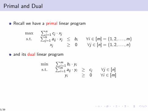
Recall we have a primal linear program
max∑n
j=1 cj · xj
s.t.∑n
j=1 aij · xj ≤ bi ∀i ∈ [m] = {1, 2, . . . ,m}xj ≥ 0 ∀j ∈ [n] = {1, 2, . . . , n}
and its dual linear program
min∑m
i=1 bi · yi
s.t.∑m
i=1 aij · yi ≥ cj ∀j ∈ [n]yi ≥ 0 ∀i ∈ [m]
3/39
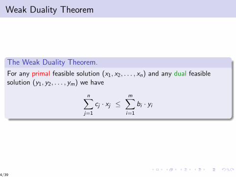
Weak Duality Theorem
The Weak Duality Theorem.
For any primal feasible solution (x1, x2, . . . , xn) and any dual feasiblesolution (y1, y2, . . . , ym) we have
n∑j=1
cj · xj ≤m∑
i=1
bi · yi
4/39

Proof of Weak Duality
Weak Duality Theorem.
For any primal feasible solution (x1, x2, . . . , xn) and any and any dualfeasible solution (y1, y2, . . . , ym) we have
∑nj=1 cj · xj ≤
∑mi=1 bi · yi .
Proof. n∑j=1
xj · cj ≤n∑
j=1
xj ·m∑
i=1
aijyi
=m∑
i=1
yi ·n∑
j=1
aijxi
≤m∑
i=1
yi · bi
5/39
Part II
Strong Duality
6/39
Strong Duality Theorem
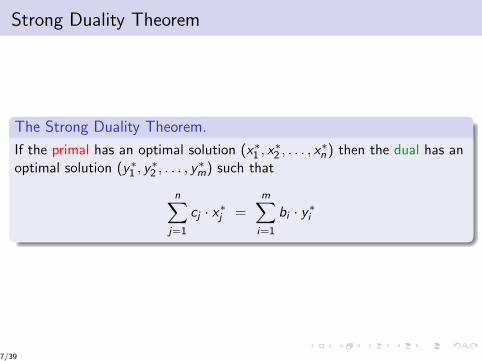
The Strong Duality Theorem.
If the primal has an optimal solution (x∗1 , x∗2 , . . . , x
∗n ) then the dual has an
optimal solution (y∗1 , y∗2 , . . . , y
∗m) such that
n∑j=1
cj · x∗j =m∑
i=1
bi · y∗i
7/39

An Example
Consider the primal
maximise 4x1 + x2 + 5x3 + 3x4
subject to x1 − x2 − x3 + 3x4 ≤ 15x1 + x2 + 3x3 + 8x4 ≤ 55−x1 + 2x2 + 3x3 − 5x4 ≤ 3
x1, x2, x3 , x4 ≥ 0
and its dual
minimise y1 + 55y2 + 3y3
subject to y1 + 5y2 − y3 ≥ 4−y1 + y2 + 2y3 ≥ 1−y1 + 3y2 + 3y3 ≥ 53y1 + 8y2 − 5y3 ≥ 3
y1, y2, y3 ≥ 0
8/39
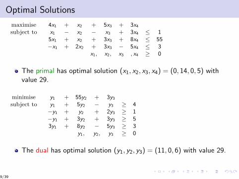
Optimal Solutions
maximise 4x1 + x2 + 5x3 + 3x4
subject to x1 − x2 − x3 + 3x4 ≤ 15x1 + x2 + 3x3 + 8x4 ≤ 55−x1 + 2x2 + 3x3 − 5x4 ≤ 3
x1, x2, x3 , x4 ≥ 0
The primal has optimal solution (x1, x2, x3, x4) = (0, 14, 0, 5) withvalue 29.
minimise y1 + 55y2 + 3y3
subject to y1 + 5y2 − y3 ≥ 4−y1 + y2 + 2y3 ≥ 1−y1 + 3y2 + 3y3 ≥ 53y1 + 8y2 − 5y3 ≥ 3
y1, y2, y3 ≥ 0
The dual has optimal solution (y1, y2, y3) = (11, 0, 6) with value 29.
9/39
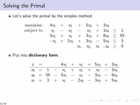
Solving the Primal
Let’s solve the primal by the simplex method.
maximise 4x1 + x2 + 5x3 + 3x4
subject to x1 − x2 − x3 + 3x4 ≤ 15x1 + x2 + 3x3 + 8x4 ≤ 55−x1 + 2x2 + 3x3 − 5x4 ≤ 3
x1, x2, x3 , x4 ≥ 0
Put into dictionary form.
z = 4x1 + x2 + 5x3 + 3x4
x5 = 1 − x1 + x2 + x3 − 3x4
x6 = 55 − 5x1 − x2 − 3x3 − 8x4
x7 = 3 + x1 − 2x2 − 3x3 + 5x4
10/39
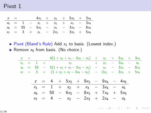
Pivot 1
z = 4x1 + x2 + 5x3 + 3x4
x5 = 1 − x1 + x2 + x3 − 3x4
x6 = 55 − 5x1 − x2 − 3x3 − 8x4
x7 = 3 + x1 − 2x2 − 3x3 + 5x4
Pivot (Bland’s Rule) Add x1 to basis. (Lowest index.)
Remove x5 from basis. (No choice.)
z = 4(1 + x2 + x3 − 3x4 − x5) + x2 + 5x3 + 3x4
x1 = 1 + x2 + x3 − 3x4 − x5
x6 = 55 − 5(1 + x2 + x3 − 3x4 − x5) − x2 − 3x3 − 8x4
x7 = 3 + (1 + x2 + x3 − 3x4 − x5) − 2x2 − 3x3 + 5x4
z = 4 + 5x2 + 9x3 − 9x4 − 4x5
x1 = 1 + x2 + x3 − 3x4 − x5
x6 = 50 − 6x2 − 8x3 + 7x4 + 5x5
x7 = 4 − x2 − 2x3 + 2x4 − x5
11/39
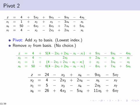
Pivot 2
z = 4 + 5x2 + 9x3 − 9x4 − 4x5
x1 = 1 + x2 + x3 − 3x4 − x5
x6 = 50 − 6x2 − 8x3 + 7x4 + 5x5
x7 = 4 − x2 − 2x3 + 2x4 − x5
Pivot: Add x2 to basis. (Lowest index.)
Remove x7 from basis. (No choice.)
z = 4 + 5(4− 2x3 + 2x4 − x5 − x7) + 9x3 − 9x4 − 4x5
x2 = 4 − 2x3 + 2x4 − x5 − x7
x1 = 1 + (4− 2x3 + 2x4 − x5 − x7) + x3 − 3x4 − x5
x6 = 50 − 6(4− 2x3 + 2x4 − x5 − x7) − 8x3 + 7x4 + 5x5
z = 24 − x3 + x4 − 9x5 − 5x7
x2 = 4 − 2x3 + 2x4 − x5 − x7
x1 = 5 − x3 − x4 − 2x5 − x7
x6 = 26 + 4x3 − 5x4 + 11x5 + 6x7
12/39
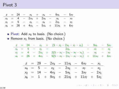
Pivot 3
z = 24 − x3 + x4 − 9x5 − 5x7
x2 = 4 − 2x3 + 2x4 − x5 − x7
x1 = 5 − x3 − x4 − 2x5 − x7
x6 = 26 + 4x3 − 5x4 + 11x5 + 6x7
Pivot: Add x4 to basis. (No choice.)
Remove x1 from basis. (No choice.)
z = 24 − x3 + (5− x3 − 2x5 − x7 − x1) − 9x5 − 5x7
x4 = 5 − x3 − 2x5 − x7 − x1
x2 = 4 − 2x3 + 2(5− x3 − 2x5 − x7 − x1) − x5 − x7
x6 = 26 + 4x3 − 5(5− x3 − 2x5 − x7 − x1) + 11x5 + 6x7
z = 29 − 2x3 − 11x5 − 6x7 − x1
x4 = 5 − x3 − 2x5 − x7 − x1
x2 = 14 − 4x3 − 5x5 − 3x7 − 2x1
x6 = 1 + 9x3 + 21x5 + 11x7 + 5x1
13/39
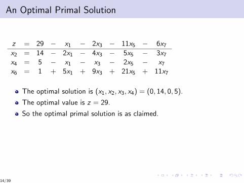
An Optimal Primal Solution
z = 29 − x1 − 2x3 − 11x5 − 6x7
x2 = 14 − 2x1 − 4x3 − 5x5 − 3x7
x4 = 5 − x1 − x3 − 2x5 − x7
x6 = 1 + 5x1 + 9x3 + 21x5 + 11x7
The optimal solution is (x1, x2, x3, x4) = (0, 14, 0, 5).
The optimal value is z = 29.
So the optimal primal solution is as claimed.
14/39
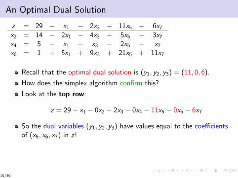
An Optimal Dual Solution
z = 29 − x1 − 2x3 − 11x5 − 6x7
x2 = 14 − 2x1 − 4x3 − 5x5 − 3x7
x4 = 5 − x1 − x3 − 2x5 − x7
x6 = 1 + 5x1 + 9x3 + 21x5 + 11x7
Recall that the optimal dual solution is (y1, y2, y3) = (11, 0, 6).
How does the simplex algorithm confirm this?
Look at the top row:
z = 29− x1 − 0x2 − 2x3 − 0x4 − 11x5 − 0x6 − 6x7
So the dual variables (y1, y2, y3) have values equal to the coefficientsof (x5, x6, x7) in z!
15/39
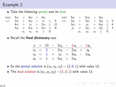
Example 2
Take the following primal and its dual
max 5x1 + 4x2 + 3x3
s.t. 2x1 + 3x2 + x3 ≤ 54x1 + x2 + 2x3 ≤ 113x1 + 4x2 + 2x3 ≤ 8
x1, x2, x3 ≥ 0
min 5y1 + 11y2 + 8y3
s.t. 2y1 + 4y2 + 3y3 ≥ 53y1 + y2 + 4y3 ≥ 4y1 + 2y2 + 2y3 ≥ 3
y1, y2, y3 ≥ 0
Recall the final dictionary was
z = 13 − 3x2 − 1x4 − 1x6
x1 = 2 − 2x2 − 2x4 + x6
x3 = 1 + x2 + 3x4 − 2x6
x5 = 1 + 5x2 + 2x4
So the primal solution is (x1, x2, x3) = (2, 0, 1) with value 13.
The dual solution is (y1, y2, y3) = (1, 0, 1) with value 13.
16/39
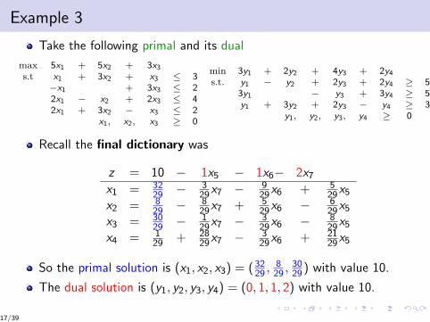
Example 3
Take the following primal and its dual
max 5x1 + 5x2 + 3x3
s.t x1 + 3x2 + x3 ≤ 3−x1 + 3x3 ≤ 22x1 − x2 + 2x3 ≤ 42x1 + 3x2 − x3 ≤ 2
x1, x2, x3 ≥ 0
min 3y1 + 2y2 + 4y3 + 2y4
s.t. y1 − y2 + 2y3 + 2y4 ≥ 53y1 − y3 + 3y4 ≥ 5y1 + 3y2 + 2y3 − y4 ≥ 3
y1, y2, y3, y4 ≥ 0
Recall the final dictionary was
z = 10 − 1x5 − 1x6− 2x7
x1 = 3229 − 3
29x7 − 929x6 + 5
29x5
x2 = 829 − 8
29x7 + 529x6 − 6
29x5
x3 = 3029 − 1
29x7 − 329x6 − 8
29x5
x4 = 129 + 28
29x7 − 329x6 + 21
29x5
So the primal solution is (x1, x2, x3) = (3229 ,
829 ,
3029) with value 10.
The dual solution is (y1, y2, y3, y4) = (0, 1, 1, 2) with value 10.
17/39
Part III
Proof of Strong Duality
18/39
Strong Duality Theorem
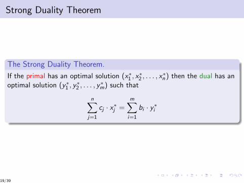
The Strong Duality Theorem.
If the primal has an optimal solution (x∗1 , x∗2 , . . . , x
∗n ) then the dual has an
optimal solution (y∗1 , y∗2 , . . . , y
∗m) such that
n∑j=1
cj · x∗j =m∑
i=1
bi · y∗i
19/39

Intuition
Look at the initial dictionary:
z = 4x1 + x2 + 5x3 + 3x4
x5 = 1 − x1 + x2 + x3 − 3x4
x6 = 55 − 5x1 − x2 − 3x3 − 8x4
x7 = 3 + x1 − 2x2 − 3x3 + 5x4
And the final dictionary:
z = 29 − x1 − 2x3 − 11x5 − 6x7
x2 = 14 − 2x1 − 4x3 − 5x5 − 3x7
x4 = 5 − x1 − x3 − 2x5 − x7
x6 = 1 + 5x1 + 9x3 + 21x5 + 11x7
The slack variable x5 appears in one constraint in the initial dictionary.
So the only way it can appear with a coefficient of 11 in the top rowof the final dictionary is if we multiplied that constraint by 11.
Similarly we must have multiplied the x7 constraint by 6.
20/39
Intuition (cont.)
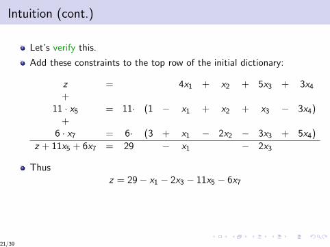
Let’s verify this.
Add these constraints to the top row of the initial dictionary:
z = 4x1 + x2 + 5x3 + 3x4
+11 · x5 = 11· (1 − x1 + x2 + x3 − 3x4)
+6 · x7 = 6· (3 + x1 − 2x2 − 3x3 + 5x4)
z + 11x5 + 6x7 = 29 − x1 − 2x3
Thusz = 29− x1 − 2x3 − 11x5 − 6x7
21/39
Intuition (cont.)
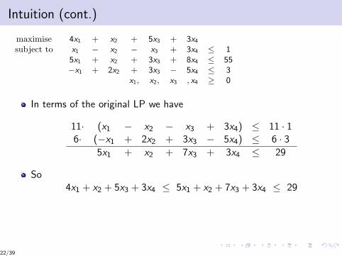
maximise 4x1 + x2 + 5x3 + 3x4
subject to x1 − x2 − x3 + 3x4 ≤ 15x1 + x2 + 3x3 + 8x4 ≤ 55−x1 + 2x2 + 3x3 − 5x4 ≤ 3
x1, x2, x3 , x4 ≥ 0
In terms of the original LP we have
11· (x1 − x2 − x3 + 3x4) ≤ 11 · 16· (−x1 + 2x2 + 3x3 − 5x4) ≤ 6 · 3
5x1 + x2 + 7x3 + 3x4 ≤ 29
So4x1 + x2 + 5x3 + 3x4 ≤ 5x1 + x2 + 7x3 + 3x4 ≤ 29
22/39
Intuition: Example 2
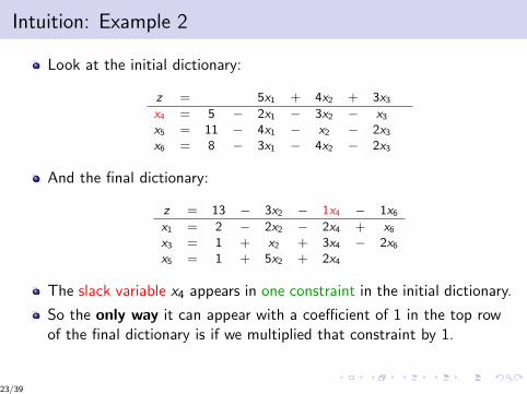
Look at the initial dictionary:
z = 5x1 + 4x2 + 3x3
x4 = 5 − 2x1 − 3x2 − x3
x5 = 11 − 4x1 − x2 − 2x3
x6 = 8 − 3x1 − 4x2 − 2x3
And the final dictionary:
z = 13 − 3x2 − 1x4 − 1x6
x1 = 2 − 2x2 − 2x4 + x6
x3 = 1 + x2 + 3x4 − 2x6
x5 = 1 + 5x2 + 2x4
The slack variable x4 appears in one constraint in the initial dictionary.
So the only way it can appear with a coefficient of 1 in the top rowof the final dictionary is if we multiplied that constraint by 1.
23/39
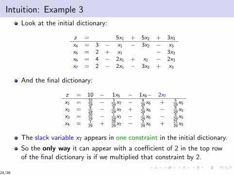
Intuition: Example 3
Look at the initial dictionary:
z = 5x1 + 5x2 + 3x3
x4 = 3 − x1 − 3x2 − x3
x5 = 2 + x1 − 3x3
x6 = 4 − 2x1 + x2 − 2x3
x7 = 2 − 2x1 − 3x2 + x3
And the final dictionary:
z = 10 − 1x5 − 1x6− 2x7
x1 = 3229
− 329
x7 − 929
x6 + 529
x5
x2 = 829
− 829
x7 + 529
x6 − 629
x5
x3 = 3029
− 129
x7 − 329
x6 − 829
x5
x4 = 129
+ 2829
x7 − 329
x6 + 2129
x5
The slack variable x7 appears in one constraint in the initial dictionary.
So the only way it can appear with a coefficient of 2 in the top rowof the final dictionary is if we multiplied that constraint by 2.
24/39
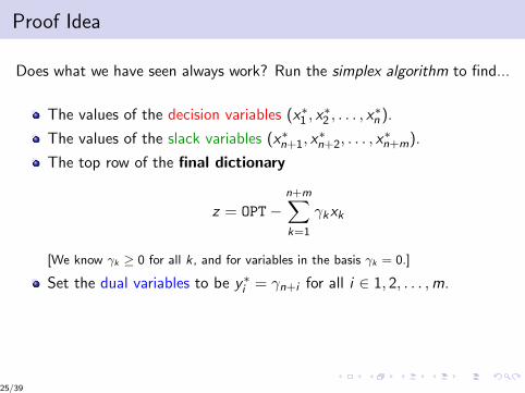
Proof Idea
Does what we have seen always work? Run the simplex algorithm to find...
The values of the decision variables (x∗1 , x∗2 , . . . , x
∗n ).
The values of the slack variables (x∗n+1, x∗n+2, . . . , x
∗n+m).
The top row of the final dictionary
z = OPT−n+m∑k=1
γkxk
[We know γk ≥ 0 for all k, and for variables in the basis γk = 0.]
Set the dual variables to be y∗i = γn+i for all i ∈ 1, 2, . . . ,m.
25/39
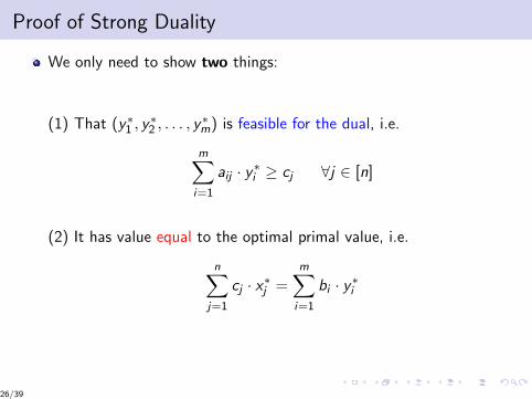
Proof of Strong Duality
We only need to show two things:
(1) That (y∗1 , y∗2 , . . . , y
∗m) is feasible for the dual, i.e.
m∑i=1
aij · y∗i ≥ cj ∀j ∈ [n]
(2) It has value equal to the optimal primal value, i.e.
n∑j=1
cj · x∗j =m∑
i=1
bi · y∗i
26/39
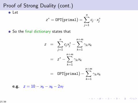
Proof of Strong Duality (cont.)Let
z∗ = OPT(primal) =n∑
j=1
cj · x∗j
So the final dictionary states that
z =n∑
j=1
cjx∗j −
n+m∑k=1
γkxk
= z∗ −n+m∑k=1
γkxk
= OPT(primal)−n+m∑k=1
γkxk
e.g. z = 10− x5 − x6 − 2x7
27/39
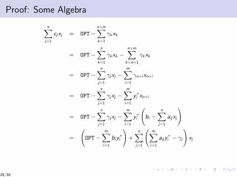
Proof: Some Algebra
nXj=1
cjxj = OPT−n+mXk=1
γkxk
= OPT−nX
k=1
γkxk −n+mX
k=n+1
γkxk
= OPT−nX
j=1
γjxj −mX
i=1
γn+ixn+i
= OPT−nX
j=1
γjxj −mX
i=1
y∗i xn+i
= OPT−nX
j=1
γjxj −mX
i=1
y∗i
bi −
nXj=1
aijxj
!
=
OPT−
mXi=1
biy∗i
!+
nXj=1
mX
i=1
aijy∗i − γj
!xj
28/39
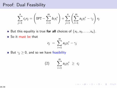
Proof: Dual Feasibility
n∑j=1
cjxj =
(OPT−
m∑i=1
biy∗i
)+
n∑j=1
(m∑
i=1
aijy∗i − γj
)xj
But this equality is true for all choices of {x1, x2, . . . , xn}.So it must be that
cj =m∑
i=1
aijy∗i − γj
But γj ≥ 0, and so we have feasibility
(2)m∑
i=1
aijy∗i ≥ cj
29/39
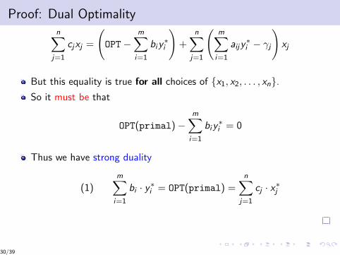
Proof: Dual Optimalityn∑
j=1
cjxj =
(OPT−
m∑i=1
biy∗i
)+
n∑j=1
(m∑
i=1
aijy∗i − γj
)xj
But this equality is true for all choices of {x1, x2, . . . , xn}.So it must be that
OPT(primal)−m∑
i=1
biy∗i = 0
Thus we have strong duality
(1)m∑
i=1
bi · y∗i = OPT(primal) =n∑
j=1
cj · x∗j
30/39

Part IV
Complementary Slackness
31/39
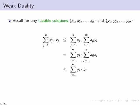
Weak Duality
Recall for any feasible solutions {x1, x2, . . . , xn} and {y1, y2, . . . , ym}
n∑j=1
xj · cj ≤n∑
j=1
xj ·m∑
i=1
aijyi
=m∑
i=1
yi ·n∑
j=1
aijxj
≤m∑
i=1
yi · bi
32/39

Strong Duality
By strong duality, we must have equalities for the optimal solutions{x∗1 , x∗2 , . . . , x∗n} and {y∗1 , y∗2 , . . . , y∗m}
n∑j=1
x∗j · cj =n∑
j=1
x∗j ·m∑
i=1
aijy∗i
=m∑
i=1
y∗i ·n∑
j=1
aijx∗j
=m∑
i=1
y∗i · bi
33/39
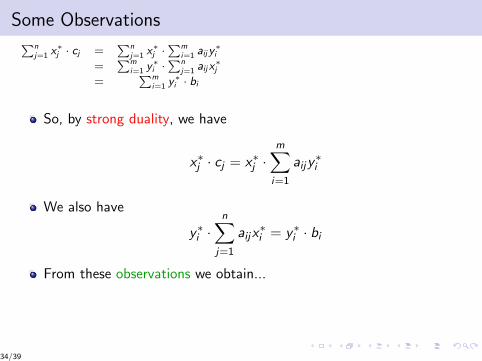
Some ObservationsPnj=1 x∗j · cj =
Pnj=1 x∗j ·
Pmi=1 aijy
∗i
=Pm
i=1 y∗i ·Pn
j=1 aijx∗j
=Pm
i=1 y∗i · bi
So, by strong duality, we have
x∗j · cj = x∗j ·m∑
i=1
aijy∗i
We also have
y∗i ·n∑
j=1
aijx∗i = y∗i · bi
From these observations we obtain...
34/39
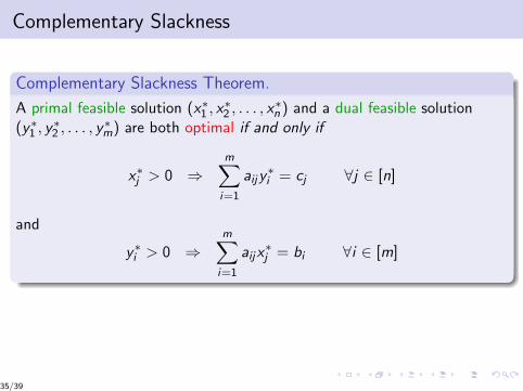
Complementary Slackness
Complementary Slackness Theorem.
A primal feasible solution (x∗1 , x∗2 , . . . , x
∗n ) and a dual feasible solution
(y∗1 , y∗2 , . . . , y
∗m) are both optimal if and only if
x∗j > 0 ⇒m∑
i=1
aijy∗i = cj ∀j ∈ [n]
and
y∗i > 0 ⇒m∑
i=1
aijx∗j = bi ∀i ∈ [m]
35/39
Part V
Consequences of Strong Duality
36/39
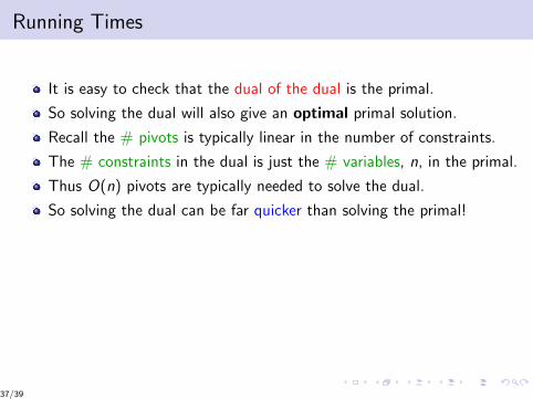
Running Times
It is easy to check that the dual of the dual is the primal.
So solving the dual will also give an optimal primal solution.
Recall the # pivots is typically linear in the number of constraints.
The # constraints in the dual is just the # variables, n, in the primal.
Thus O(n) pivots are typically needed to solve the dual.
So solving the dual can be far quicker than solving the primal!
37/39
Dual Variables
We have seen many examples where the dual problem often has anice combinatorial meaning.
In economic problems often the primal variables correspond toallocations and the dual variables to prices.
38/39
Certificates
The simplex algorithm gives us a certificate of optimality.
Given a primal solution x∗ the dual solution y∗ proves x∗ is optimal.[So always check that the x∗ you found is optimal!]
So a certificate let’s us know when to stop searching.
Certificates seem fundamental in assessing the hardness of problems....
39/39