10. support vector machines -...
TRANSCRIPT
10. Support Vector Machines
Foundations of Machine LearningCentraleSupélec — Fall 2017
Chloé-Agathe AzencotCentre for Computational Biology, Mines ParisTech

2
Learning objectives● Define a large-margin classifier in the separable case.● Write the corresponding primal and dual optimization
problems.● Re-write the optimization problem in the case of non-
separable data.● Use the kernel trick to apply soft-margin SVMs to non-
linear cases.● Define kernels for real-valued data, strings, and graphs.

3
The linearly separable case:hard-margin SVMs

4
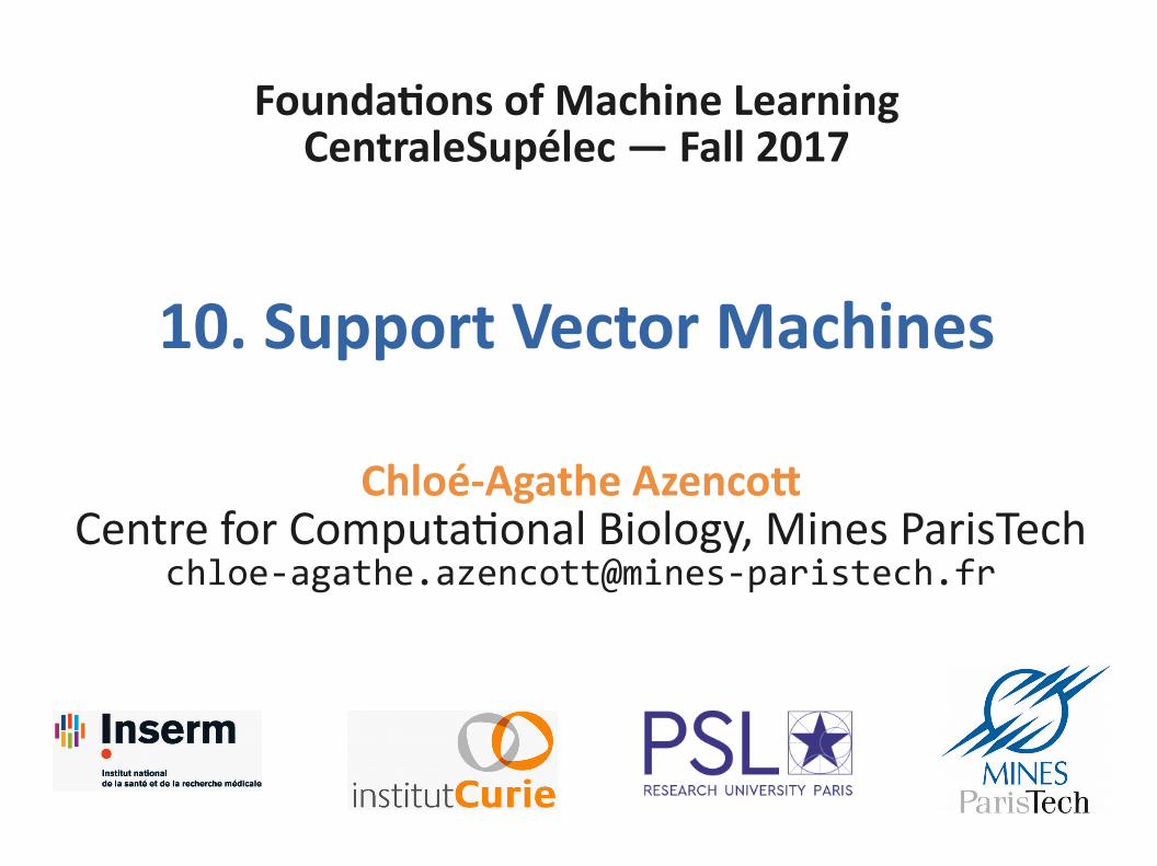
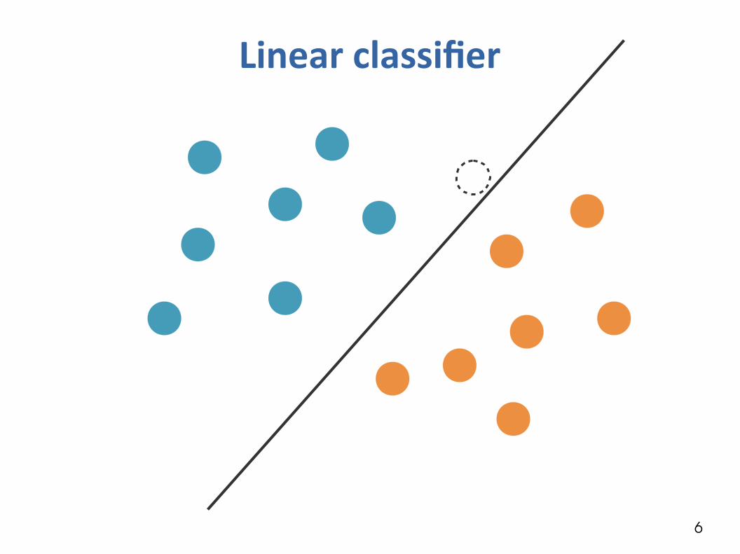
Linear classifier
Assume data is linearly separable: there exists a line that separates + from -

5
Linear classifier
6
Linear classifier

7
Linear classifier
8
Linear classifier

9
Linear classifier

10
Linear classifier
11
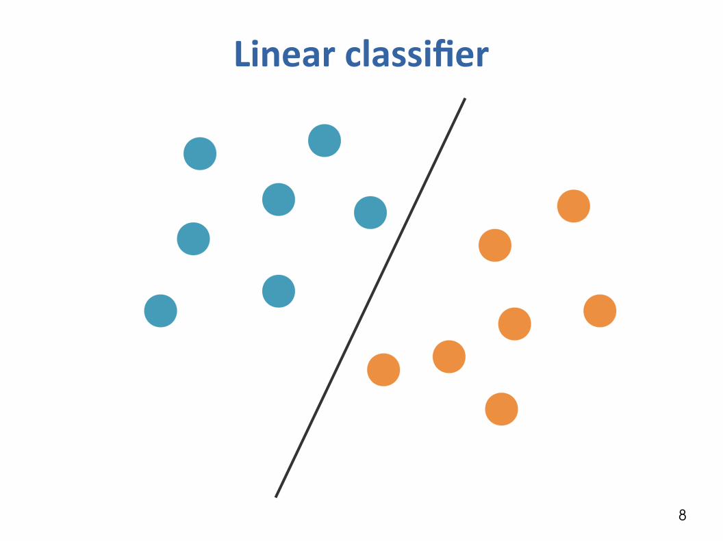
Linear classifier
Which one is beter?

12
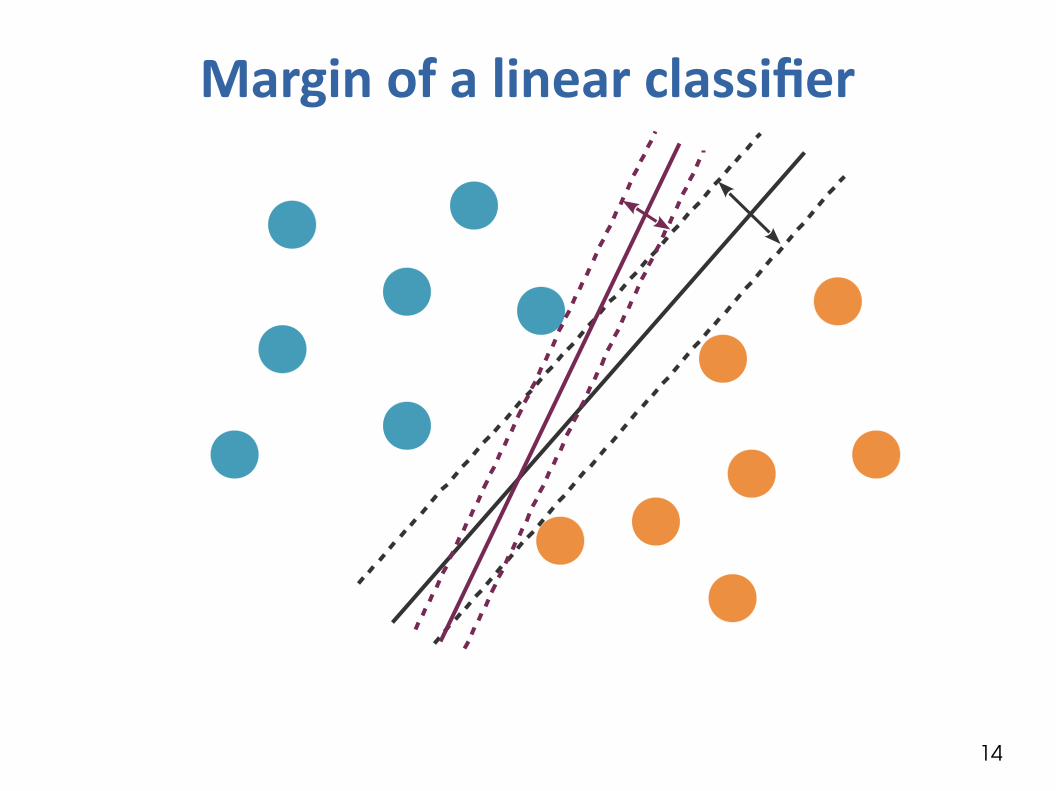
Margin of a linear classifier
Margin: Twice the distance from the separating hyperplane to the closest training point.

13
Margin of a linear classifier
14
Margin of a linear classifier
15
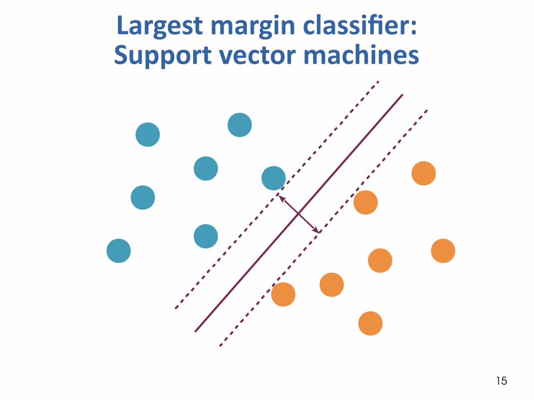
Largest margin classifier:Support vector machines

16
Support vectors
17
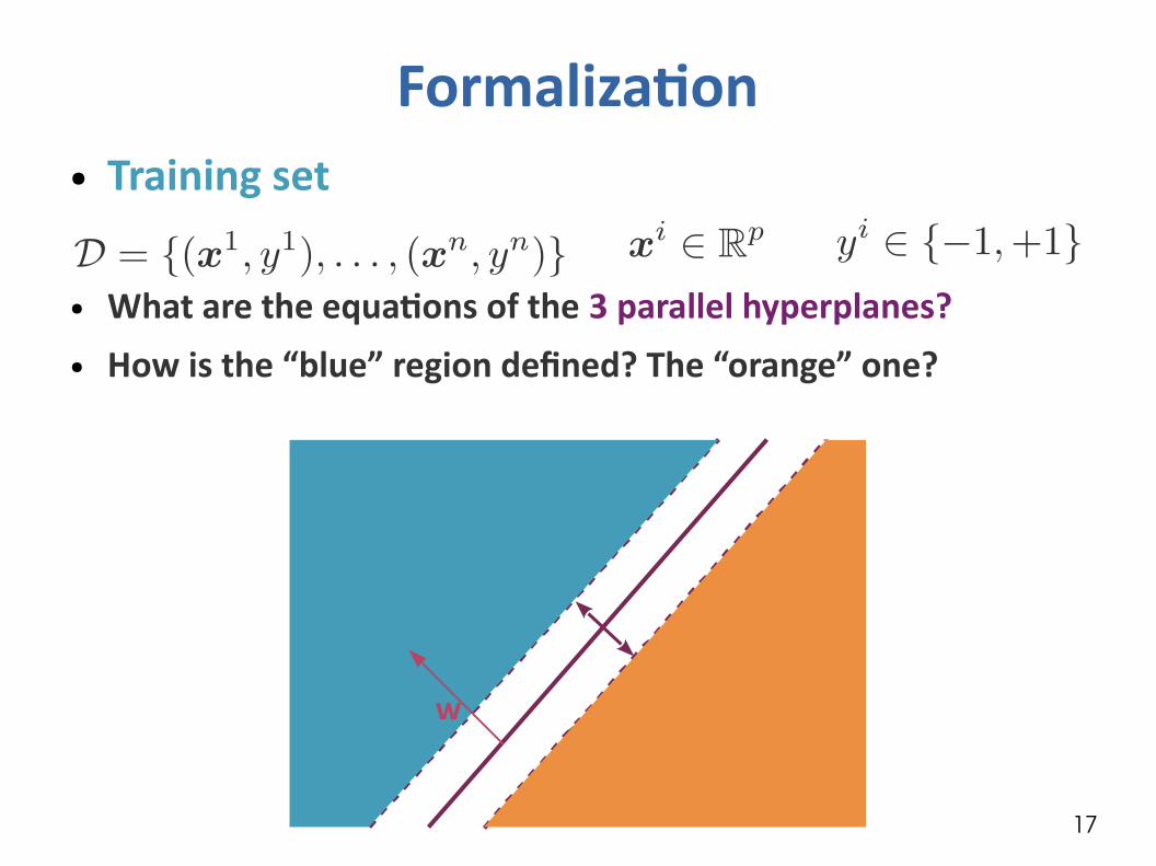
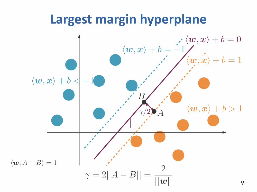
Formalization● Training set
● What are the equations of the 3 parallel hyperplanes?● How is the “blue” region defined? The “orange” one?
w
18
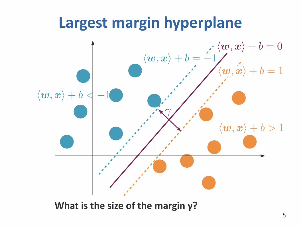
Largest margin hyperplane
What is the size of the margin γ?
19
Largest margin hyperplane

20
Optimization problem● Training set
● Assume the data to be linearly separable
● Goal: Find that define the hyperplane with largest margin.

21
Optimization problem● Margin maximization:
minimize ● Correct classification of the training points:
– For positive examples:
– For negative examples:
– Summarized as ?

22
Optimization problem● Margin maximization:
minimize ● Correct classification of the training points:
– For positive examples:
– For negative examples:
– Summarized as:● Optimization problem:

23
● Find that minimize under the n constraints
● We introduce one dual variable αi for each constraint (i.e. each training point)
● Lagrangian:
Optimization problem
?

24
● Find that minimize under the n constraints
● We introduce one dual variable αi for each constraint (i.e. each training point)
● Lagrangian:
Optimization problem

25
Lagrange dual of the SVM
● Lagrange dual function:
● Lagrange dual problem:
● Strong duality: Under Slater’s conditions, the optimum of the primal is the optimum of the dual.
The function to optimize is convex and the equality constraints are affine.
26
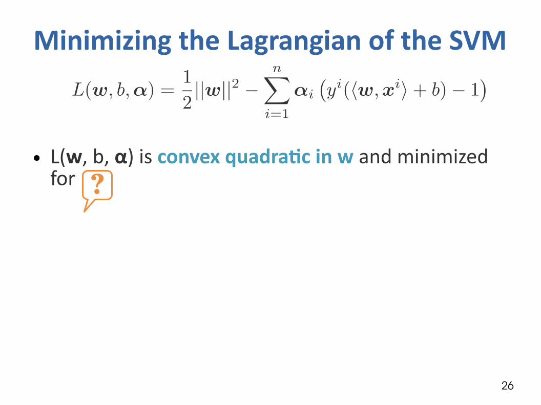
Minimizing the Lagrangian of the SVM
● L(w, b, α) is convex quadratic in w and minimized for
● L(w, b, α) is affine in b. Its minimum is except if
?

27
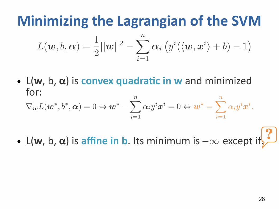
Minimizing the Lagrangian of the SVM
● L(w, b, α) is convex quadratic in w and minimized for:
● L(w, b, α) is affine in b. Its minimum is except if:
28
Minimizing the Lagrangian of the SVM
● L(w, b, α) is convex quadratic in w and minimized for:
● L(w, b, α) is affine in b. Its minimum is except if:?

29
Minimizing the Lagrangian of the SVM
● L(w, b, α) is convex quadratic in w and minimized for:
● L(w, b, α) is affine in b. Its minimum is except if:

30
SVM dual problem
● Lagrange dual function:
● Dual problem: maximize q(α) subject to α ≥ 0.Maximizing a quadratic function under box constraints can be solved efficiently using dedicated software.

31
Optimal hyperplane● Once the optimal α* is found, we recover (w*, b*)
● Determining b*:
– Closest positive point to the separating hyperplane: verifies
– Closest negative point to the separating hyperplane:verifies
● The decision function is hence:

32
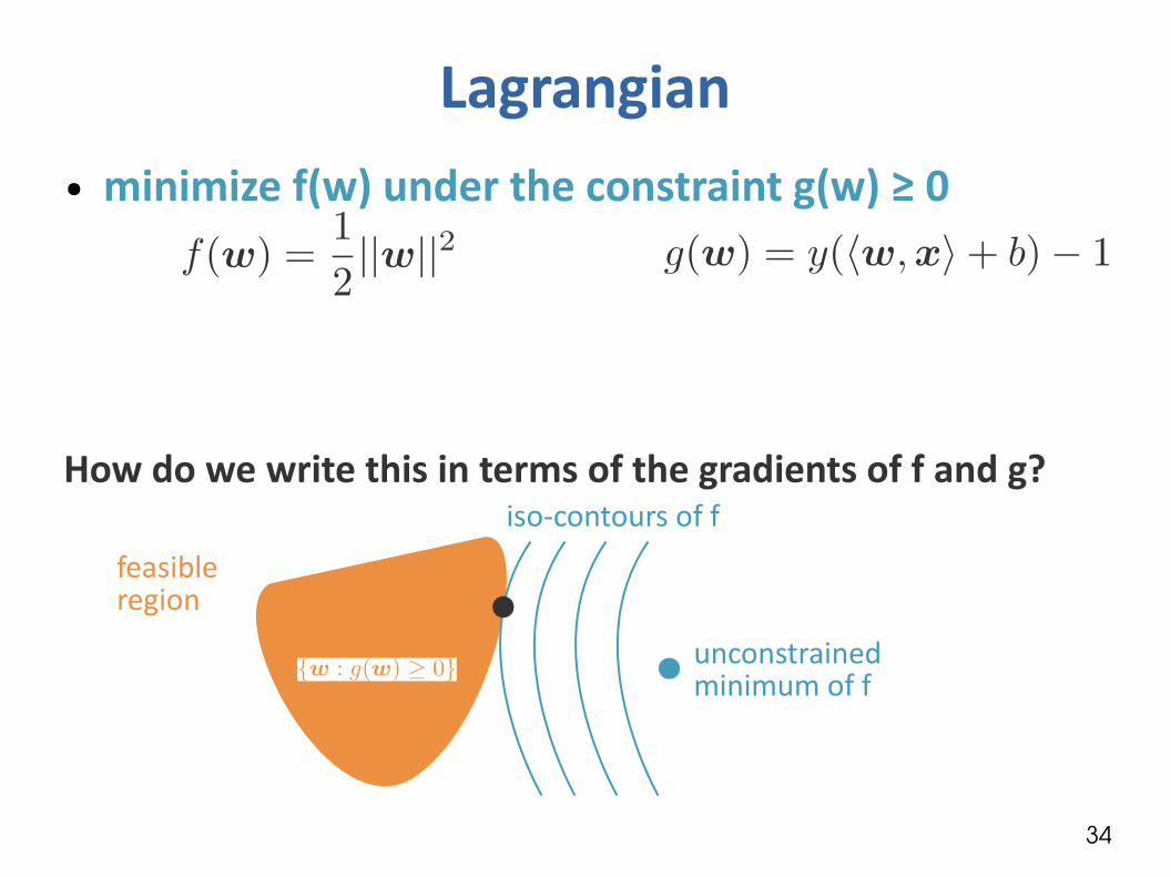
Lagrangian● minimize f(w) under the constraint g(w) ≥ 0
How do we write this in terms of the gradients of f and g?
abusive notation: g(w, b)

33
Lagrangian● minimize f(w) under the constraint g(w) ≥ 0
feasible region
iso-contours of f
unconstrained minimum of f
If the minimum of f(w) doesn't lie in the feasible region,where's our solution?
34
Lagrangian● minimize f(w) under the constraint g(w) ≥ 0
feasible region
iso-contours of f
unconstrained minimum of f
How do we write this in terms of the gradients of f and g?

35
Lagrangian● minimize f(w) under the constraint g(w) ≥ 0
feasible region
iso-contours of f
unconstrained minimum of f
How do we write this in terms of the gradients of f and g?
36
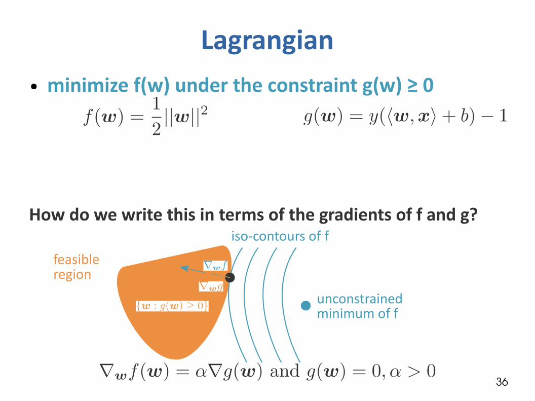
Lagrangian● minimize f(w) under the constraint g(w) ≥ 0
feasible region
iso-contours of f
unconstrained minimum of f
How do we write this in terms of the gradients of f and g?

37
Lagrangian● minimize f(w) under the constraint g(w) ≥ 0
Case 1: the unconstraind minimum lies in the feasible region.Case 2: it does not.
How do we summarize both cases?
38
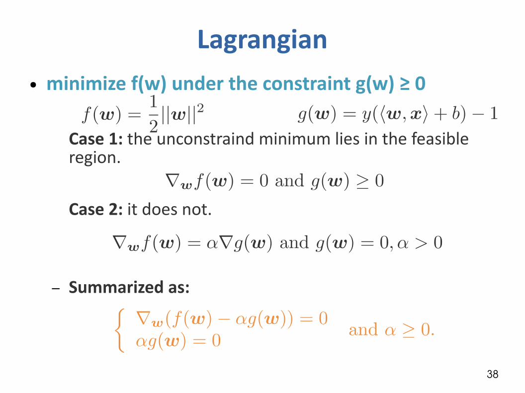
● minimize f(w) under the constraint g(w) ≥ 0
Case 1: the unconstraind minimum lies in the feasible region.
Case 2: it does not.
– Summarized as:
Lagrangian

39
● minimize f(w) under the constraint g(w) ≥ 0
Lagrangian:α is called the Lagrange multiplier.
Lagrangian

40
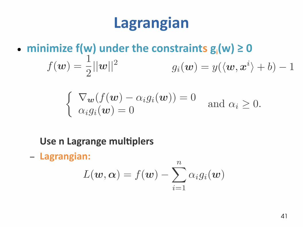
● minimize f(w) under the constraints gi(w) ≥ 0
How do we deal with n constraints?
Lagrangian
41
● minimize f(w) under the constraints gi(w) ≥ 0
Use n Lagrange multiplers – Lagrangian:
Lagrangian

42
Support vectors● Karun-Kush-Tucker conditions:
Either αi = 0 (case 1) or gi=0 (case 2)
Case 1:Case 2:
feasible region
iso-contours of f
unconstrained minimum of f

43
Support vectors
α = 0α > 0
44
The non-linearly separable case: soft-margin SVMs.
45
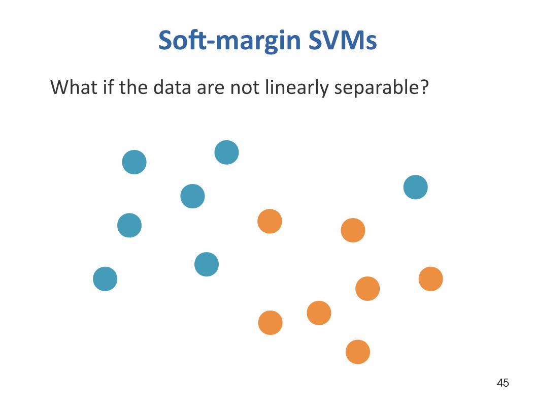
Soft-margin SVMsWhat if the data are not linearly separable?

46
Soft-margin SVMs

47
Soft-margin SVMs

48
Soft-margin SVMs● Find a trade-off between large margin and few
errors.
What does this remind you of?

49
SVM error: hinge loss
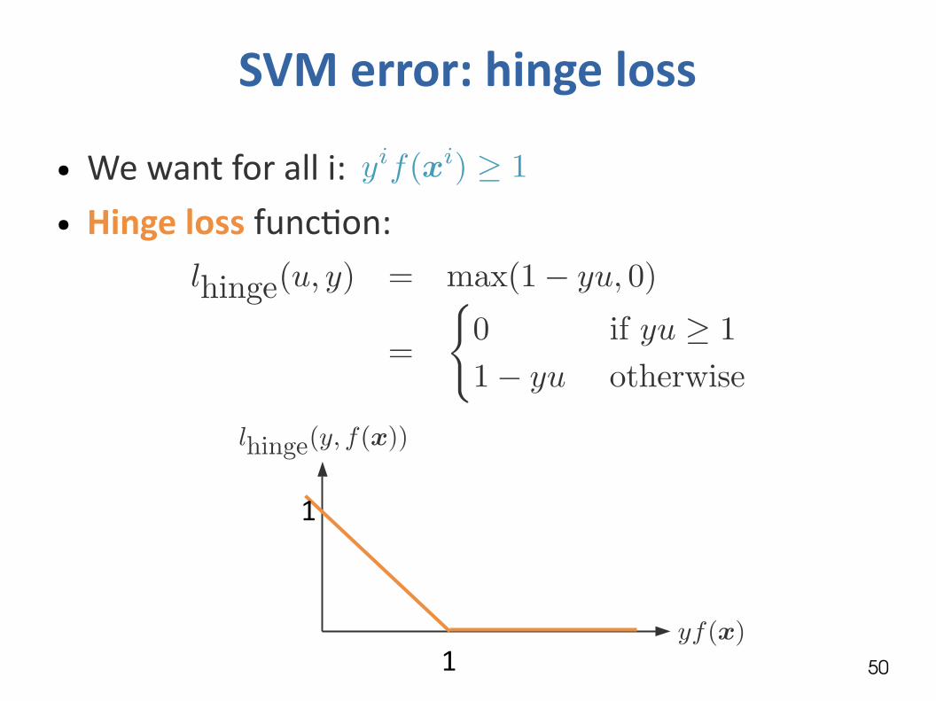
● We want for all i:● Hinge loss function:
What's the shape of the hinge loss?
50
SVM error: hinge loss
● We want for all i:● Hinge loss function:
1
1

51
Soft-margin SVMs● Find a trade-off between large margin and few
errors.
● Error:
● The soft-margin SVM solves:
52
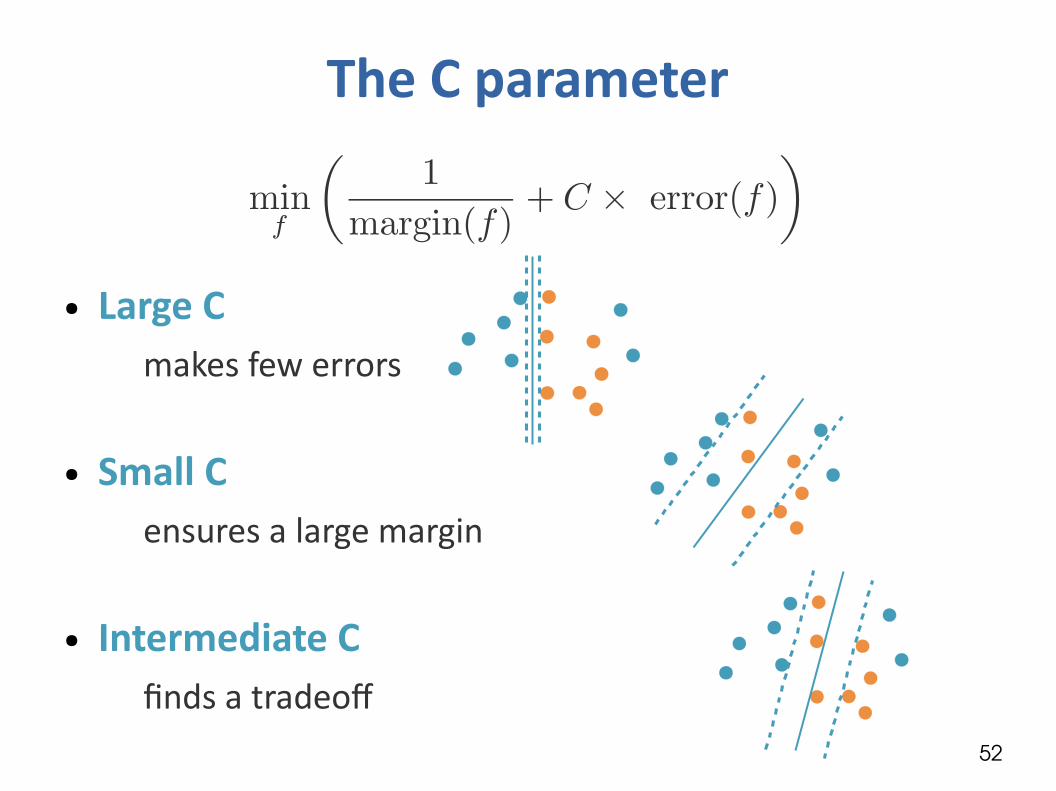
The C parameter
● Large Cmakes few errors
● Small Censures a large margin
● Intermediate Cfinds a tradeoff

53
It is important to control CPr
edic
tion
erro
r
C
On training data
On new data

54
Slack variables
is equivalent to:
slack variable:distance btw y.f(x) and 1

55
● Primal
● Lagrangian
● Min the Lagrangian (partial derivatives in w, b, ξ)
● KKT conditions
Lagrangian of the soft-margin SVM
56
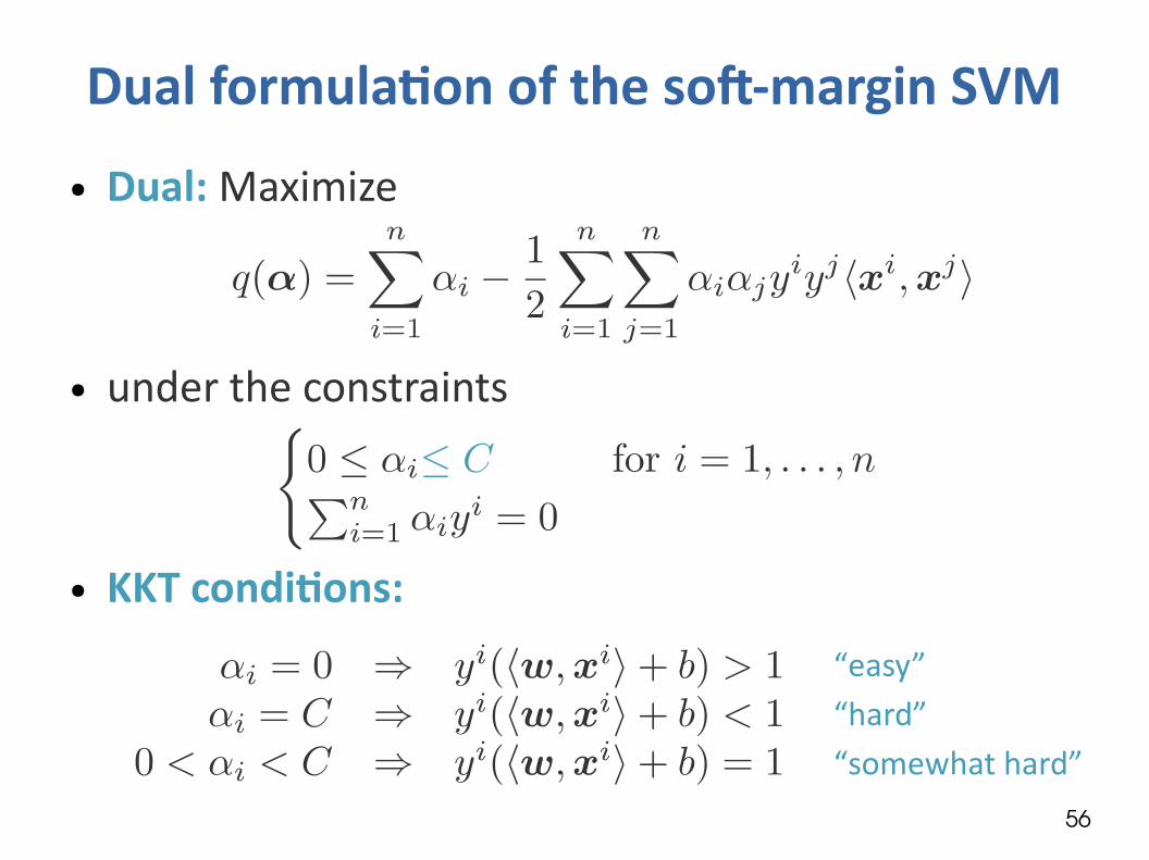
Dual formulation of the soft-margin SVM
● Dual: Maximize
● under the constraints
● KKT conditions:
“easy” “hard” “somewhat hard”

57
Support vectors of the soft-margin SVM
α = 00< α < C
α = C
58
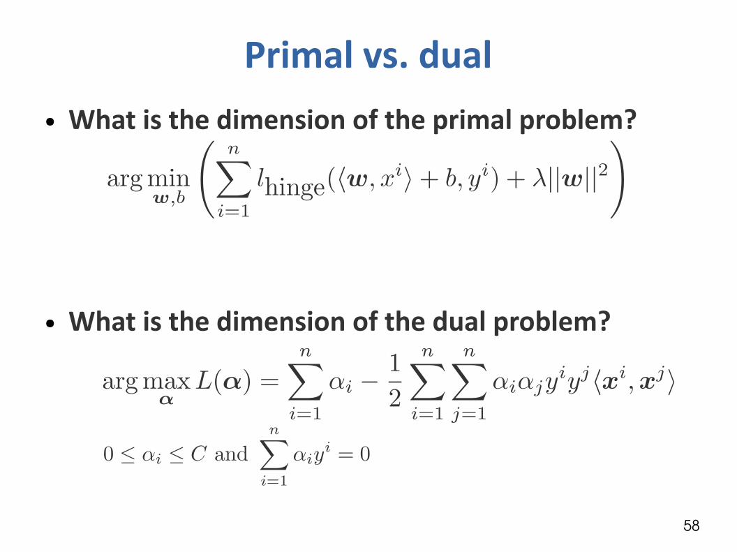
Primal vs. dual● What is the dimension of the primal problem?
● What is the dimension of the dual problem?

59
Primal vs. dual● Primal: (w, b) has dimension (p+1).
Favored if the data is low-dimensional.
● Dual: α has dimension n.
Favored is there is litle data available.

60
The non-linear case: kernel SVMs.

61
Non-linear SVMs
62
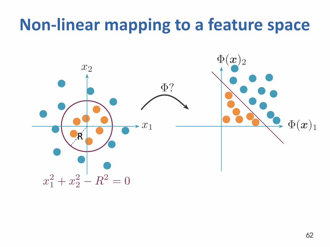
Non-linear mapping to a feature space
R

63
Non-linear mapping to a feature space
R R2

64
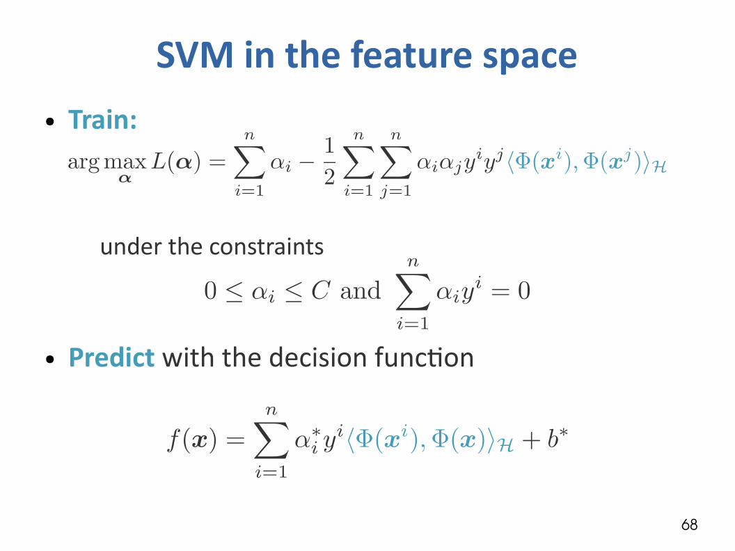
SVM in the feature space● Train:
under the constraints
● Predict with the decision function

65
KernelsFor a given mapping
from the space of objects X to some Hilbert space H, the kernel between two objects x and x' is the inner product of their images in the feature spaces.
● E.g.
● Kernels allow us to formalize the notion of similarity.
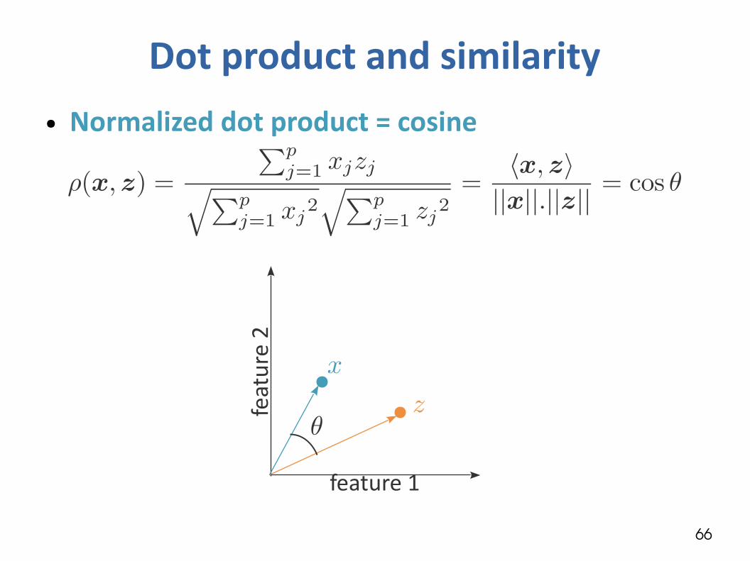
66
Dot product and similarity● Normalized dot product = cosine
feat
ure
2
feature 1

67
Kernel trick
● Many linear algorithms (in particular, linear SVMs) can be performed in the feature space H without explicitly computing the images φ(x), but instead by computing kernels K(x, x')
● It is sometimes easy to compute kernels which correspond to large-dimensional feature spaces: K(x, x') is often much simpler to compute than φ(x).
68
SVM in the feature space● Train:
under the constraints
● Predict with the decision function

69
SVM with a kernel● Train:
under the constraints
● Predict with the decision function
70
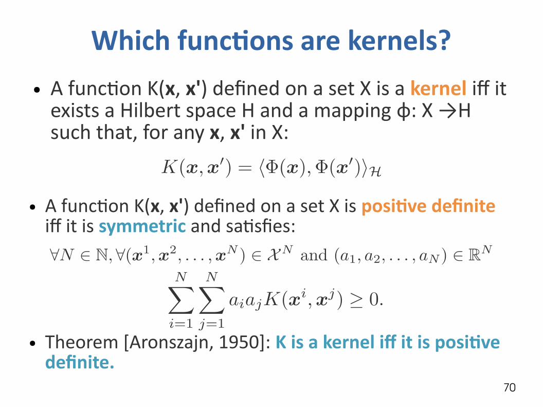
Which functions are kernels?● A function K(x, x') defined on a set X is a kernel iff it
exists a Hilbert space H and a mapping φ: X →H such that, for any x, x' in X:
● A function K(x, x') defined on a set X is positive definite iff it is symmetric and satisfies:
● Theorem [Aronszajn, 1950]: K is a kernel iff it is positive definite.
71
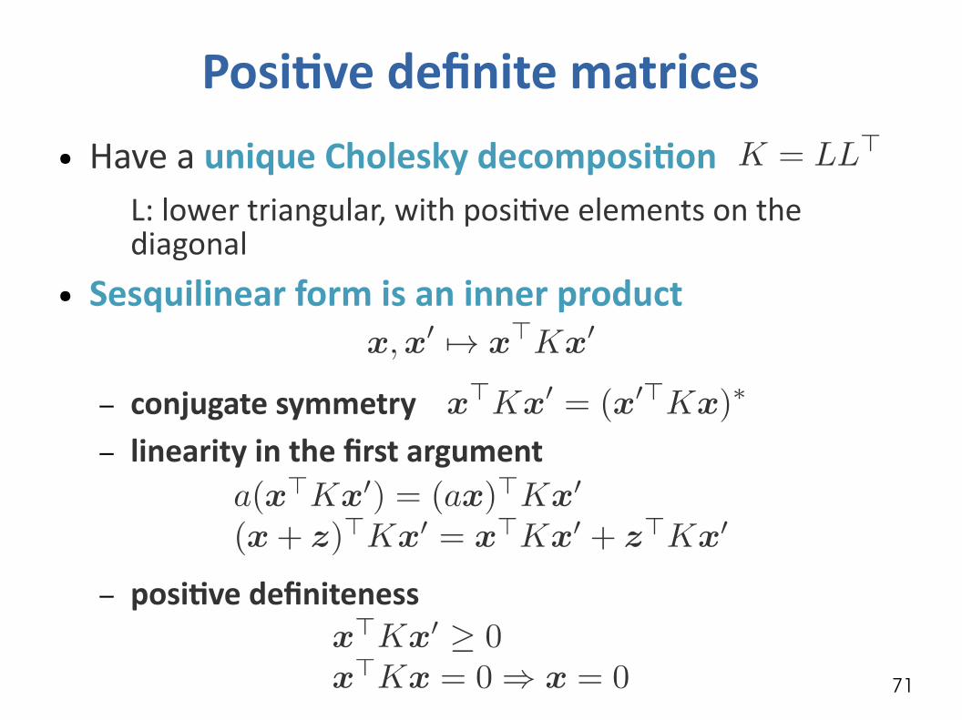
Positive definite matrices● Have a unique Cholesky decomposition
L: lower triangular, with positive elements on the diagonal
● Sesquilinear form is an inner product
– conjugate symmetry– linearity in the first argument
– positive definiteness

72
Polynomial kernels
Compute ?

73
Polynomial kernels
More generally, for
is an inner product in a feature space of all monomials of degree up to d.

74
Gaussian kernel
What is the dimension of the feature space?

75
Gaussian kernel
The feature space has infinite dimension.

76

77
Toy example

78
Toy example: linear SVM
79
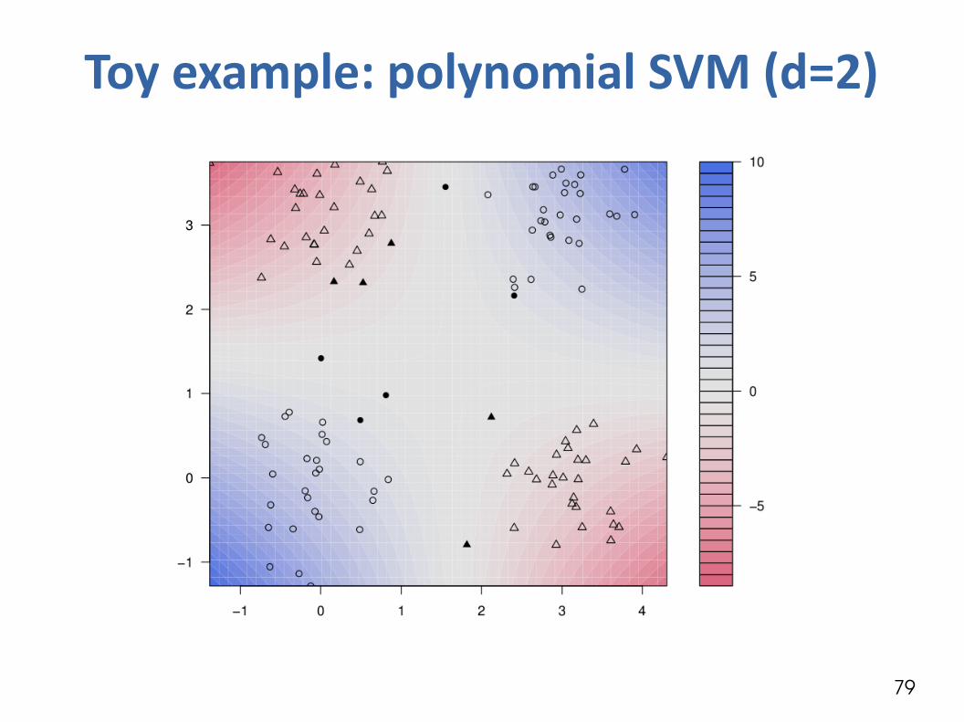
Toy example: polynomial SVM (d=2)
80
Kernels for strings

81
Protein sequence classificationGoal: predict which proteins are secreted or not, based on their sequence.

82
Substring-based representations● Represent strings based on the presence/absence of
substrings of fixed length.
Strings of length k?

83
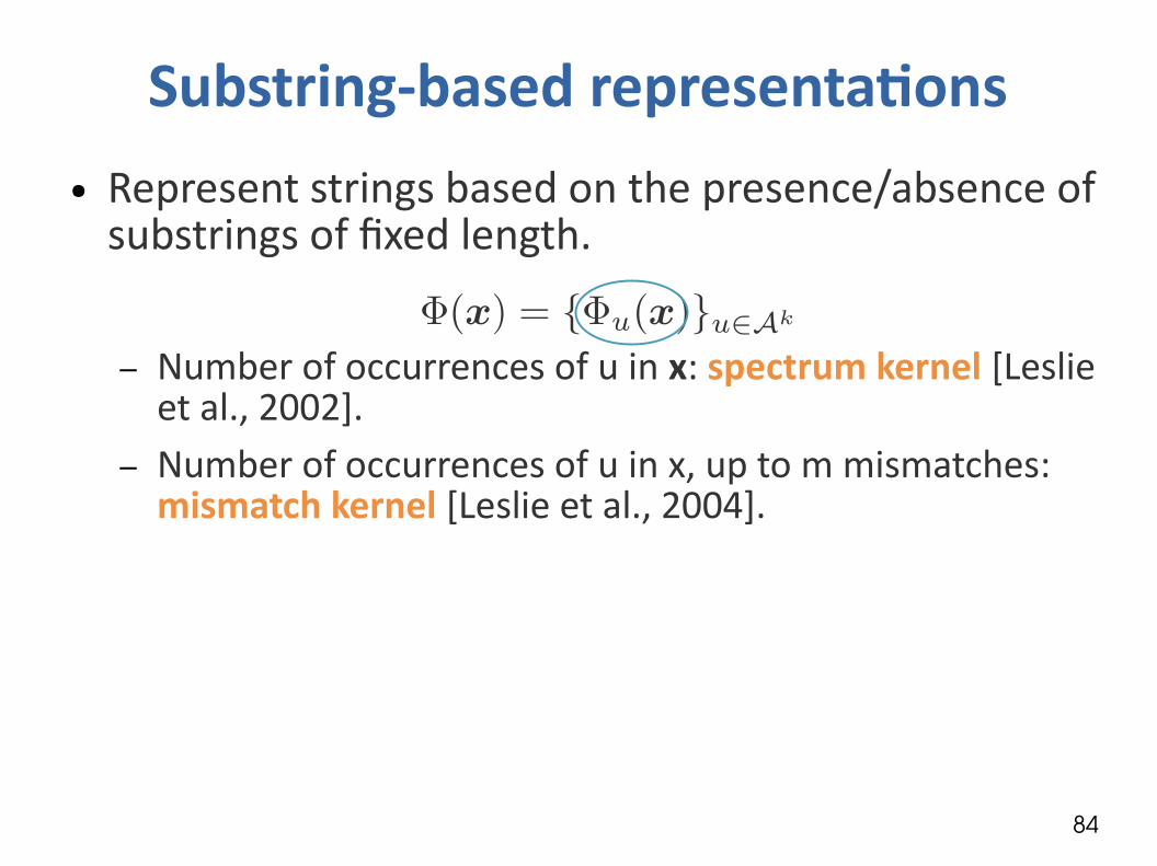
Substring-based representations● Represent strings based on the presence/absence of
substrings of fixed length.
– Number of occurrences of u in x: spectrum kernel [Leslie et al., 2002].
84
Substring-based representations● Represent strings based on the presence/absence of
substrings of fixed length.
– Number of occurrences of u in x: spectrum kernel [Leslie et al., 2002].
– Number of occurrences of u in x, up to m mismatches: mismatch kernel [Leslie et al., 2004].

85
Substring-based representations● Represent strings based on the presence/absence of
substrings of fixed length.
– Number of occurrences of u in x: spectrum kernel [Leslie et al., 2002].
– Number of occurrences of u in x, up to m mismatches: mismatch kernel [Leslie et al., 2004].
– Number of occcurrences of u in x, allowing gaps, with a weight decaying exponentially with the number of gaps: substring kernel [Lohdi et al., 2002].

86
Spectrum kernel
● Implementation:– Formally, a sum over |Ak|terms– How many non-zero terms in ?
?

87
Spectrum kernel
● Implementation:– Formally, a sum over |Ak|terms– At most |x| - k + 1 non-zero terms in – Hence: Computation in O(|x|+|x'|)
● Prediction for a new sequence x:
Write f(x) as a function of only |x|-k+1 weights.?

88
Spectrum kernel
● Implementation:– Formally, a sum over |Ak|terms– At most |x| - k + 1 non-zero terms in – Hence: Computation in O(|x|+|x'|)
● Fast prediction for a new sequence x:
89
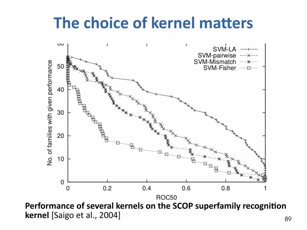
The choice of kernel maters
Performance of several kernels on the SCOP superfamily recognition kernel [Saigo et al., 2004]

90
Kernels for graphs

91
Graph data● Molecules
● Images
[Harchaoui & Bach, 2007]

92
Subgraph-based representations
0 1 1 0 0 1 0 0 0 1 0 1 0 0 1
no occurrenceof the 1st feature
1+ occurrencesof the 10th feature

93
Tanimoto & MinMax● The Tanimoto and MinMax similarities are kernels
94
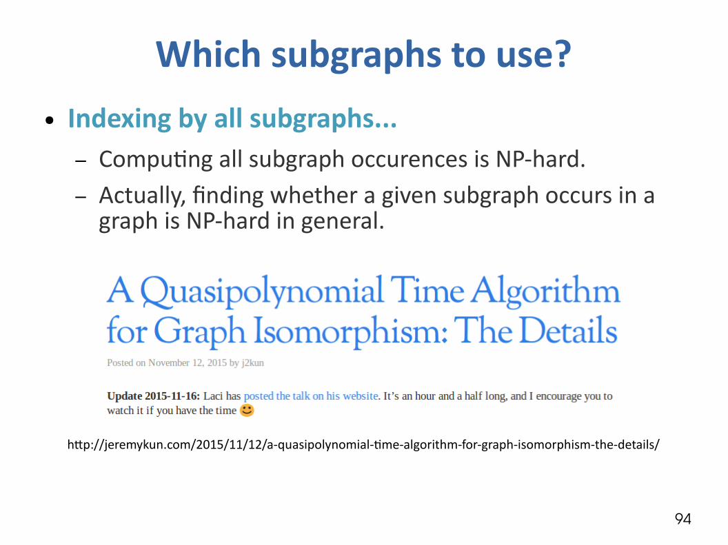
Which subgraphs to use?● Indexing by all subgraphs...
– Computing all subgraph occurences is NP-hard.– Actually, finding whether a given subgraph occurs in a
graph is NP-hard in general.
http://jeremykun.com/2015/11/12/a-quasipolynomial-time-algorithm-for-graph-isomorphism-the-details/
95
Which subgraphs to use?● Specific subgraphs that lead to computationally
efficient indexing:– Subgraphs selected based on domain knowledge
E.g. chemical fingerprints– All frequent subgraphs [Helma et al., 2004]– All paths up to length k [Nicholls 2005]– All walks up to length k [Mahé et al., 2005]– All trees up to depth k [Rogers, 2004]– All shortest paths [Borgwardt & Kriegel, 2005]– All subgraphs up to k vertices (graphlets) [Shervashidze
et al., 2009]

96
Which subgraphs to use?
Path of length 5 Walk of length 5 Tree of depth 2

97
Which subgraphs to use?
[Harchaoui & Bach, 2007]
Paths
Walks
Trees

98
The choice of kernel maters
Predicting inhibitors for 60 cancer cell lines [Mahé & Vert, 2009]

99
The choice of kernel maters
[Harchaoui & Bach, 2007]
● COREL14: 1400 natural images, 14 classes● Kernels: histogram (H), walk kernel (W), subtree kernel
(TW), weighted subtree kernel (wTW), combination (M).

100
Summary● Linearly separable case: hard-margin SVM● Non-separable, but still linear: soft-margin SVM● Non-linear: kernel SVM● Kernels for
– real-valued data– strings– graphs.
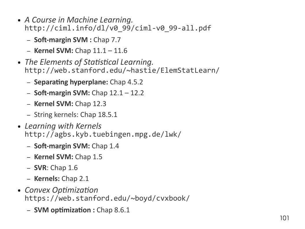
101
● A Course in Machine Learning. http://ciml.info/dl/v0_99/ciml-v0_99-all.pdf
– Soft-margin SVM : Chap 7.7– Kernel SVM: Chap 11.1 – 11.6
● The Elements of Statistical Learning. http://web.stanford.edu/~hastie/ElemStatLearn/
– Separating hyperplane: Chap 4.5.2– Soft-margin SVM: Chap 12.1 – 12.2– Kernel SVM: Chap 12.3 – String kernels: Chap 18.5.1
● Learning with Kernels http://agbs.kyb.tuebingen.mpg.de/lwk/
– Soft-margin SVM: Chap 1.4– Kernel SVM: Chap 1.5– SVR: Chap 1.6– Kernels: Chap 2.1
● Convex Optimization https://web.stanford.edu/~boyd/cvxbook/
– SVM optimization : Chap 8.6.1

102
Practical maters● Preparing for the exam
– Previous exams with solutions on the course website● Next week: special session! 2 x 1.5 hrs
– Introduction to artificial neural networks– Introduction to deep learning and Tensorflow (J. Boyd)
Jupyter notebook will be available for download– Deep learning for bioimaging (P. Naylor)

103
Lab● Redefining cross_validate

104
Linear SVM
The data is not easily separated by a hyperplane
Support vectors are either correctly classified points that support the margin or errors.
Many support vectors suggest the data is not easy to separate and there are many erros.
105
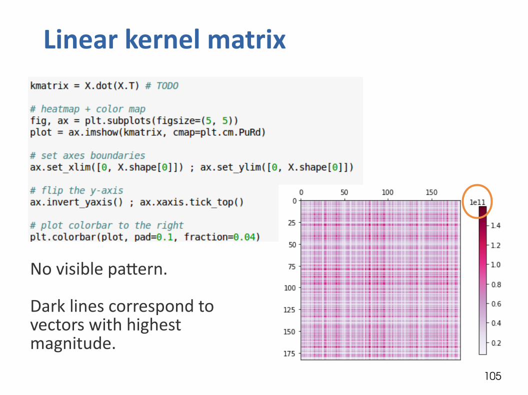
Linear kernel matrix
No visible pattern.
Dark lines correspond to vectors with highest magnitude.
106
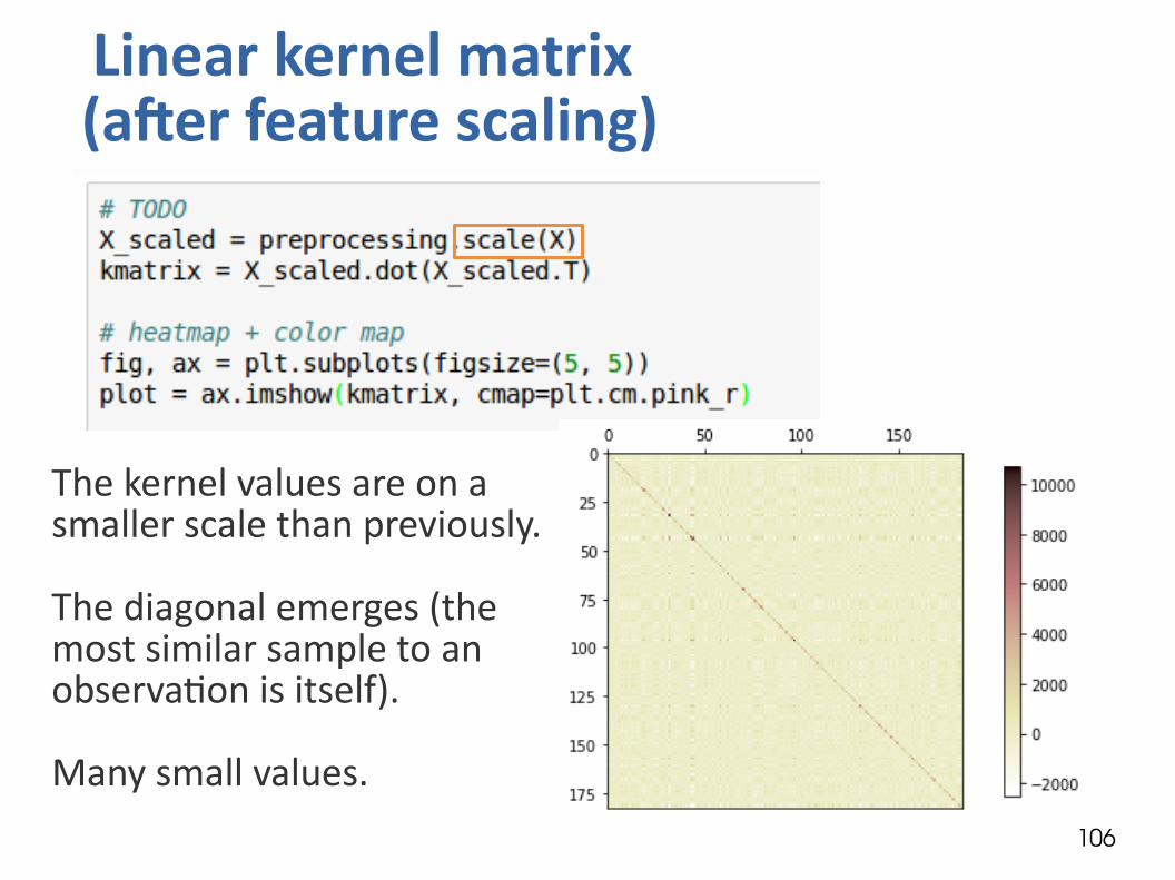
Linear kernel matrix (after feature scaling)
The kernel values are on a smaller scale than previously.
The diagonal emerges (the most similar sample to an observation is itself).
Many small values.

107
108
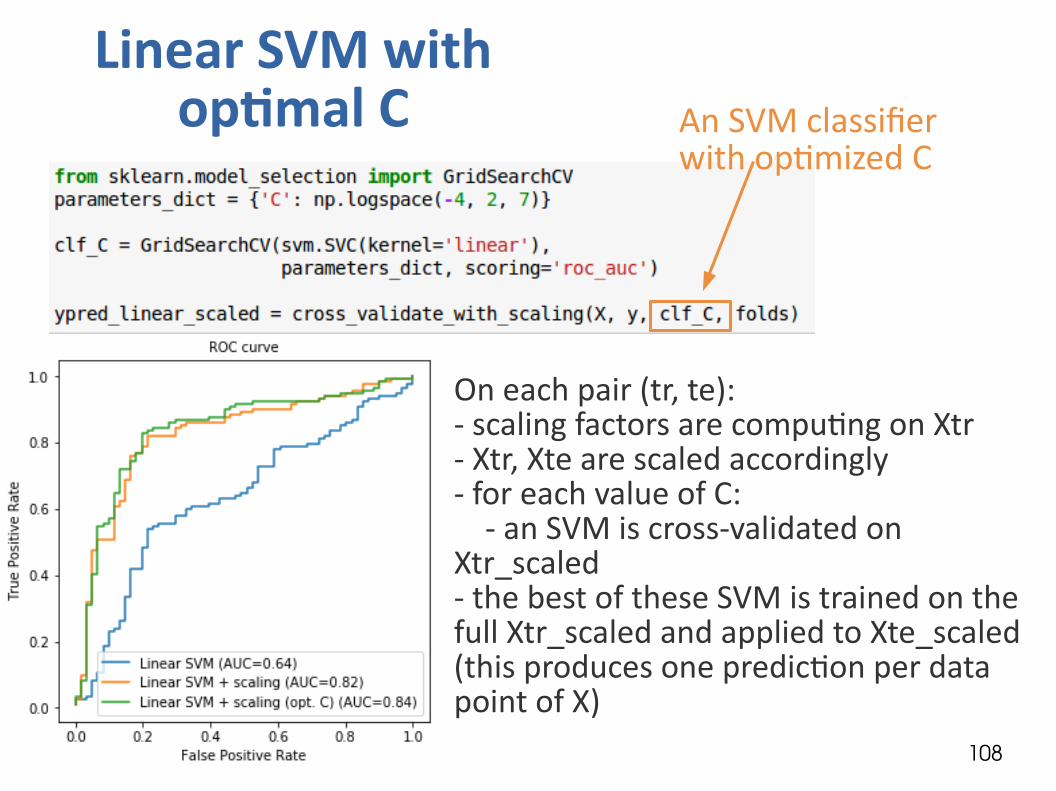
Linear SVM with optimal C An SVM classifier
with optimized C
On each pair (tr, te):- scaling factors are computing on Xtr- Xtr, Xte are scaled accordingly- for each value of C: - an SVM is cross-validated on Xtr_scaled- the best of these SVM is trained on the full Xtr_scaled and applied to Xte_scaled (this produces one prediction per data point of X)
109
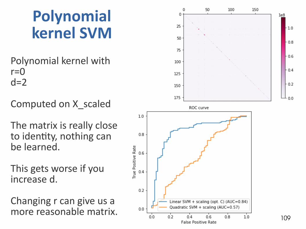
Polynomial kernel SVM
Polynomial kernel with r=0d=2
Computed on X_scaled
The matrix is really close to identity, nothing can be learned.
This gets worse if you increase d.
Changing r can give us a more reasonable matrix.

110
r=1000000Almost all 1s
r=100000r=10000
r=1000r=100r=10The kernel matrix is almost the identity matrix
Reasonable range of values for r

111
● For a fair comparison with the linear kernel, cross-validate C and r.
● For r, use a logspace between 10000 and 100000 based on your observation of the kernel matrix.

112
Gaussian kernel SVM● What values of gamma should we use? Start by
spreading out values.
● When gamma > 1e-2, the kernel matrix is close to the identity.
● When gamma = 1e-5, the kernel matrix is getting close to a matrix of all 1s.
● If we choose gamma much smaller, the kernel matrix is going to be so close to a matrix of all 1s the SVM won’t learn well.

113
Gaussian kernel SVM● What values of gamma should we use? Start by
spreading out values.
● The kernel matrix is more reasonable when gamma is between 5e-5 and 5e-4.
114
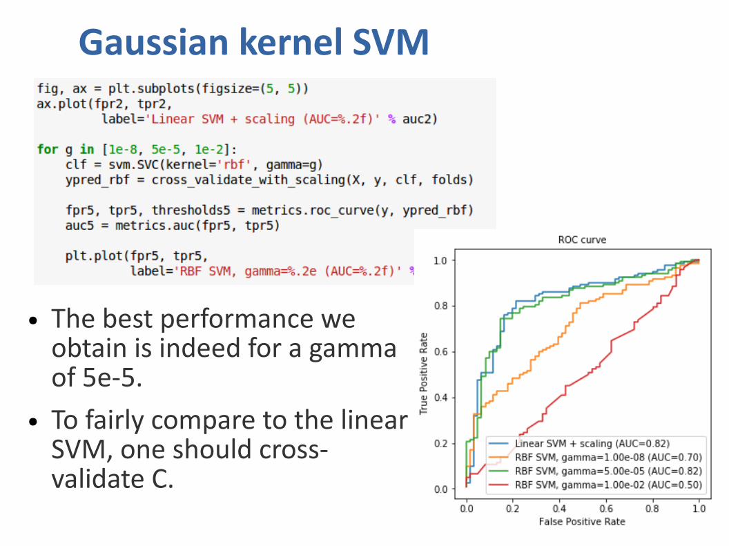
Gaussian kernel SVM
● The best performance we obtain is indeed for a gamma of 5e-5.
● To fairly compare to the linear SVM, one should cross-validate C.
115
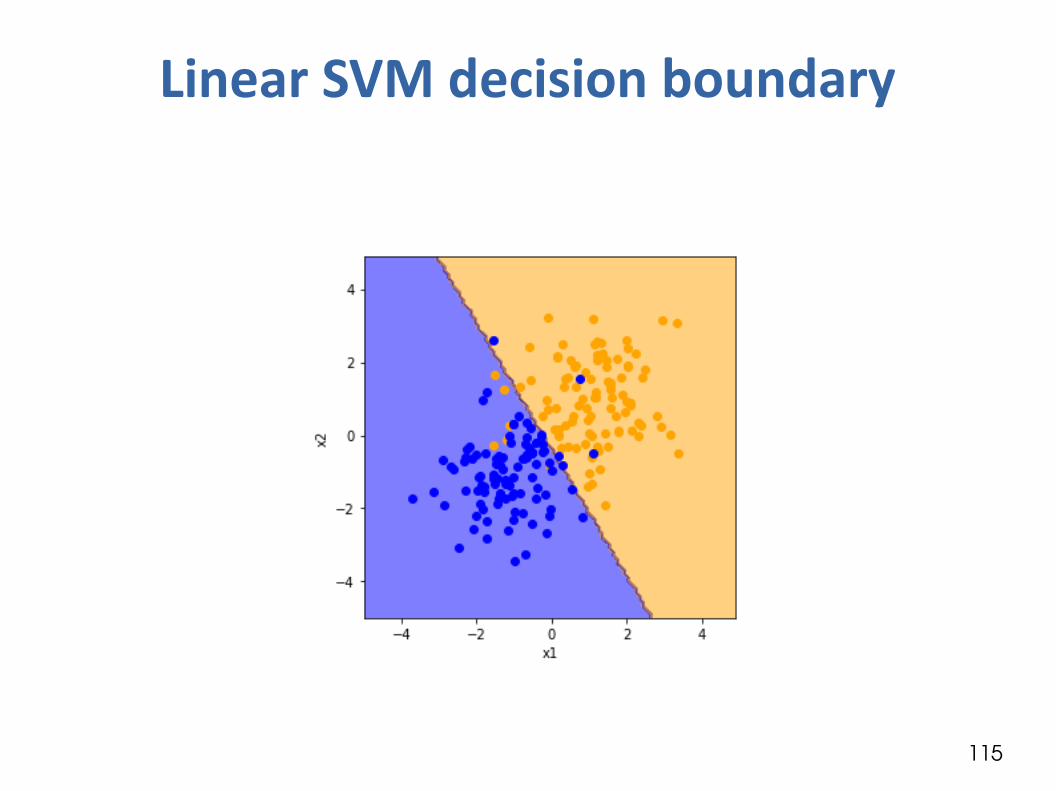
Linear SVM decision boundary

116
Quadratic SVM decision boundary
117
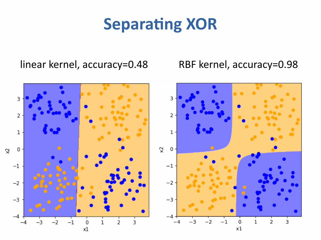
Separating XOR
RBF kernel, accuracy=0.98linear kernel, accuracy=0.48