1

A Better Bayesian Convergence Theorem1

James Hawthorne

University of Oklahoma

(hawthorne@ou.edu)

Introduction

Any inductive logic worthy of the name ought to supply a measure of evidential support that, as a reasonable amount of evidence accumulates, tends to indicate that false hypotheses are probably false and that true hypotheses are probably true. Is there an inductive logic that can be shown to possess this delightful property? I will argue that a proper construal of Bayesian confirmation provides just this kind of truth-value indicating measure. I aim to convince you of this by explicating a so-called Bayesian Convergence Theorem. The theorem will show that under some rather sensible conditions, if a hypothesis h is false, its Bayesian posterior probabilities will very probably approach the falsehood indicating value 0 as evidence accumulates; and as the posterior probabilities of false competitors fall, the posterior probability of the true hypothesis heads towards 1.

1. Bayesian Background

1.1 Formalism

To begin with, consider some exhaustive set {h1, h2,…} of alternative (i.e., mutually incompatible) hypotheses or theories about some subject matter. The set of alternatives may be very simple – e.g. {“the patient is infected with HIV”, “the patient is free of HIV”} – or it may consist of several alternatives − e.g. several alternative gravitational theories. In general, there may be either a finite or an infinite number such alternatives under consideration. They may all be considered at once, or they may be constructed and compared over a long historical period. One may even think of the set as consisting of all logically possible alternative hypotheses about a given subject matter expressible in a given language (e.g. all possible theories of the origin and evolution of the universe expressible in English and mathematics). Although the idealized case of testing all possible alternative hypotheses is generally impractical, the way the logic works in this ideal limit may have interesting implications for more realistic cases, where only a relatively

2

small number of alternatives are considered at a time. Indeed, it turns out that the logic works in much the same way for any number of alternative hypotheses.

If the set of alternative hypotheses is finite, it may contain a catch-all hypothesis hK that says that none of the other hypotheses are true − e.g., “none of the known diseases are causing this patient’s symptoms”. That is, when only some number u of explicit alternative hypotheses is under consideration, hK is the sentence (~h1·…·~hu).

Evidence for scientific hypotheses consists of the results of specific experiments or observations. For a given experiment or observation, let ‘c’ represent a description of the conditions under which it is performed, and let ‘e’ represent a description of the evidential outcome that results from condition c. In addition, let ‘b’ represent explicit background information and auxiliary hypotheses that are not at issue in the assessment of the hypotheses hi, but mediate the connection between the hypotheses and the evidence. The idea is that when hi is deductively related to the evidence, there will often be background information and auxiliary hypotheses that mediate the logical entailments; and ‘b’ represents these. Thus, in the case of deductively related evidence, either hi·b·c �e or hi·b·c �~e.

1.2 Likelihoods

I will call the probability function that measure the Bayesian support of hypotheses by evidence Bayesian support functions or inductive support functions. For inductive support functions, the likelihoods carry the empirical import of hypotheses. A likelihood is a support function probability of form P[e | hi·b·c]. It expresses how likely the evidence e is on a given hypothesis. (Bayesians often refer to the probability of an evidence statement on a hypothesis, P[e | h·b·c], as the likelihood of the hypothesis. This is a somewhat confusing convention since it is clearly the evidence that is made likely to whatever degree by the hypothesis. So, I will disregard the usual convention here. Also, presentations of Bayesian inference often suppress c and b, and simply write ‘P[e | h]’. But c and b are important parts of the logic of the likelihoods. So I will continue to make them explicit.) If a hypothesis together with auxiliaries and observation conditions deductively entails an evidence claim, the axioms of probability make the corresponding likelihood objective in the sense that every support function must agree on its values: P[e | hi·b·c] = 1 if hi·b·c � e; P[e | hi·b·c] = 0 if hi·b·c �~e. However, in many cases the hypothesis hi will not be deductively related to the evidence, but will instead only “statistically imply” the evidence. This may happen in two different ways. Either hi may itself be an explicitly probabilistic or statistical hypothesis, or it may happen that an auxiliary statistical hypothesis, as part of background b, connects hi to the evidence.

Likelihoods that arise in either of these ways (i.e. from explicit statistical claims entailed by the hypotheses being tested, or from explicit statistical claims in the background information that ties

3

the hypotheses to the evidence) are often called direct inference likelihoods. Such likelihoods appear to be quite objective. So it seems reasonable to suppose that all support functions should agree on their values, just as all support functions agree on likelihoods when evidence is logically entailed. Such likelihoods are logical in an extended, non-deductive sense. Indeed, some logicians have attempted to spell out the logic of direct inferences in terms of the logical form of the sentences involved. (These attempts have not been wholly satisfactory thus far. But research on this continues. For an illuminating discussion of the logic of direct inference and the difficulties involved in providing a formal account, see the series of papers (Levi, 1977), (Kyburg, 1978) and (Levi, 1978). (Levi, 1980) develops a fairly sophisticated Bayesian approach.) But regardless of whether that project succeeds, it seems reasonable to take likelihoods of this sort to have highly objective or intersubjectively agreed values.

Not all likelihoods of interest in scientific confirmational contexts are direct inferences, because not all such likelihoods are warranted deductively or by explicitly stated statistical claims. Nevertheless, the likelihoods that relate hypotheses to evidence in scientific contexts will often have objective or intersubjectively agreed values. That is, although a wide variety of different support functions P�, P� ,…, P�, etc., may be needed to represent the various “inductive proclivities” of the members of a scientific community, all should agree (at least approximately) on the values of the likelihoods of evidence claims given by specific hypotheses. For, the likelihoods represent the empirical content of a hypothesis − what the hypothesis says about evidence claims. So, the empirical objectivity of a science relies on a high degree of objectivity or intersubjective agreement among scientists on the numerical values of likelihood.

To see the point, imagine what a science would be like if scientists disagreed widely about the values of likelihoods. Each practitioner interprets a specific theory to say quite different things about which of various possible evidence statements are likely to be true. Suppose, for example, that on scientist �’s reading, theory h1 says that evidence event e is quite likely; but his colleague � reads the empirical import of h1 differently, as implying that e is rather unlikely. In addition, � reads competing theory h2 as saying that e is highly unlikely; whereas � may take h2 to say that e is very likely. Thus, while � finds that e furnishes strong evidential support for h1 over h2 (because P�[e | h1·b·cn] >> P�[e | h2·b·c]), his colleague � takes e to show just the opposite — that e furnishes strong support for h2 over h1 (since P�[e | h1·b·c] << P�[e | h2·b·c]). If this kind of thing were to occur often or for significant evidence claims in a scientific domain, it would make a shambles of the empirical objectivity of that science. It would completely undermine the empirical testability of its hypotheses and theories. Under such circumstances, although each scientist employs the same theoretical sentences to express a given theory h, each understands the empirical import of these sentences so differently that h as understood by � is effectively (i.e., empirically) a different theory than h as understood by �. Thus, the empirical objectivity of the sciences requires that experts should be in close agreement about the values of the likelihoods for evidence claims employed to confirm or refute theories. Let us mark the

4

agreement among agents in a given scientific community on the values of likelihoods by dropping the subscript ‘�’, ‘�’, etc., from expressions that represent them.

(Actually, although agreement on likelihoods is highly desirable, all that is required for empirical testability is agreement, or near agreement, on the values of ratios of likelihoods. However, in many scientific contexts objective or intersubjectively agreed likelihoods are readily available. The main ideas behind inductive logic will be more easily explained if, for now, we treat only those contexts were objective or intersubjectively agreed likelihoods are available. Towards the end of the paper we will see how this supposition may be relaxed − that much the same logic continues to apply in contexts where likelihoods may not possess objective or intersubjectively agreed values.)

One more notational wrinkle involving likelihoods before moving on: Scientific hypotheses are usually tested by a sequence of experiments or observations obtained over time. Let the series of sentences c1,c2,…,cn, describe the conditions under which these experiments or observations are conducted. They result in outcomes described by corresponding sentences e1, e2,…,en. Let us abbreviate the conjunction of the first n experimental or observational condition statements by ‘cn’, and let us abbreviate the conjunction of descriptions of their outcomes by ‘en’. Thus, for a stream of n observations or experiments and their outcomes, the likelihoods take form P[en | hi·b·cn] = r, for appropriate r between 0 and 1.

1.3 Posterior Probabilities and Prior Probabilities

In Bayesian inductive logic the evaluation of a hypothesis on evidence is represented by its posterior probability, P�[hi | b·cn·e n]. The posterior probability of a hypothesis might well be called its posterior plausibility. It represents the net plausibility of the hypothesis resulting from the combination of evidence together with non-evidential plausibility considerations. The likelihoods are the means through which evidence contributes to posterior probabilities. But another factor, the prior probability of the hypothesis (on background b), P�[hi | b], also makes a contribution. It represents the weight of all non-evidential plausibility considerations on which posterior plausibilities may depend. Posterior probabilities depend only on the values of (ratios of) likelihoods and on the values of prior probabilities.

In the evidential evaluation of scientific theories, prior probabilities often represent assessments by agents of non-evidential, conceptually motivated plausibility weightings among hypotheses. However, because such plausibility assessments tend to vary among agents, critics often brand them as merely subjective, and take their role in Bayesian induction to be highly problematic. Bayesian inductivists counter that such assessments often play an important role in the sciences, especially when there is insufficient evidence to distinguish among some of the alternative hypotheses. And, they argue, the epithet merely subjective is unwarranted. Such plausibility

5

assessments are often backed by extensive arguments that may draw on forceful conceptual considerations.

Consider, for example, the kind of plausibility arguments that have been brought to bear on the various interpretations of quantum theory (e.g., those related to the measurement problem). These arguments go to the heart of conceptual issues that were central to the development of the theory. Indeed, these issues were in many cases first raised by the scientists who have made the greatest contributions to the theory’s development, in their attempts to get a conceptual hold on the theory and its implications. And although disagreements remain, such arguments seem to play a legitimate role in the assessment of alternative views when distinguishing evidence has yet to be found.

More generally, scientists often bring plausibility arguments to bear in assessing their views. And although such arguments are seldom decisive, they may bring the scientific community into widely shared agreement, especially regarding the implausibility of some logically possible alternatives. This seems to be the primary epistemic role of the thought experiment. It is arguably a virtue of Bayesian induction that it provides a place for such assessments to figure into the full evaluations of hypotheses. So, although prior probabilities are subjective in the sense that agents may disagree on the relative strengths of plausibility arguments, and thus on the ultimate plausibilities of various alternative hypothesis, priors are far from being mere subjective whims. Moreover, Bayesian induction shows how, when sufficient empirical evidence becomes available, such plausibility assessments are “washed out” or overridden by the evidence. (We'll see how this works below.) From the perspective of Bayesian inductive logic, the point of some of the so-called Bayesian convergence results is to provide assurance that priors will very probably be overridden by evidence whenever hypotheses are empirically distinct to a significant degree.

(Note: if one wishes to avoid prior plausibility considerations, and only attend to the import of the empirical evidence itself, this is easily accomplished. It turns out that the likelihood ratios, P[en | hj·b·cn] / P[e n | hi·b·cn] provide a pure measure of how strongly the evidence supports hi as compared to its support for hj, “untainted” by prior plausibility considerations. This will become clear in a moment.)

Some Bayesian logicians have held that posterior probabilities of hypotheses should be determined by logical form alone. The idea was that the direct inference likelihoods might reasonably be specified in terms of logical form; so if logical form might be made to determine the values of prior probabilities as well, then inductive logic would be fully “formal” in the same way that deductive logic is “formal”. Most logicians now take the project to have failed because of a fatal flaw with the whole idea that reasonable prior probabilities can be made to depend on logical form alone. Semantic content should matter. Goodmanian grue-predicates provide one

6

way to illustrate this point.2 So it seems that prior probabilities of hypothesis should depend on semantic content rather than merely on syntactic form.

We will return to the discussion of prior probabilities after seeing their role in the logic of Bayesian induction.

1.4 Bayes’s Theorem

Bayesian inductive logic takes its name from Bayes’s Theorem, a theorem of probability theory that expresses how evidence, through the likelihoods, combines with prior plausibility assessments to produce posterior plausibility values for hypotheses. Let’s now consider several forms of Bayes’s Theorem. The simplest form is this:

P�[hi | b·cn·en] = (P[en | hi·b·cn] · P�[hi | b] / P�[en | b·cn]) · (P�[cn | hi·b] / P�[cn | b])

= P[en | hi·b·cn] · P�[hi | b] / P�[en | b·cn], if P�[cn | hi·b] = P�[cn | b].

This equation expresses the posterior probability of hi, P�[hi | b·cn·en], in terms of the likelihood of the evidence on the hypothesis (together with background and observation conditions), P[en | hi·b·cn], the prior probability of the hypothesis (given background conditions), P�[hi | b], and the simple probability of the evidence (given background and observation conditions), P�[en | b·cn]. This latter probability is sometimes called the expectedness of the evidence.

This version of Bayes’s Theorem also includes a term, (P�[cn | hi·b]/P �[cn | b]), that represents the ratio of the likelihood of the experimental conditions on the hypothesis (together with background) to the “likelihood” of the experimental conditions on the background alone. Bayes’s Theorem is usually expressed in a way that suppresses this factor. This is usually done by building cn into the background b − sometimes explicitly, but usually only implicitly. But if cn is built into b, then technically b must change as new evidence is accumulated. Better to make the factor explicit, and see how to deal with it logically. Indeed, arguably this factor should be 1, or near 1, since the truth of the hypothesis at issue should not significantly affect how likely it is that the experimental conditions are satisfied. When alternative hypotheses say something significantly different about the likelihoods of “experimental conditions”, such conditions should be included as part of the evidential outcomes e.

Both the prior probability of the hypothesis and the expectedness tend to be “subjective”. That is, various agents from the same scientific community may legitimately disagree on what values these factors should take. Bayesian logicians usually accept the subjectivity of the prior probabilities of hypotheses, but they find the subjectivity of the expectedness more troubling. However, this problem is easily finessed.

7

The subjective expectedness of the evidence may be circumvented by considering a ratio form of Bayes’s Theorem, a form that compares hypotheses one pair at a time:

P�[hj | b·cn·en] P[en | hj·b·cn] P�[hj | b] P�[cn | hj·b] (1) −−−−−−−−−− = −−−−−−−−−− · −−−−−−− · −−−−−−−− P�[hi | b·cn·en] P[en | hi·b·cn] P�[hi | b] P�[cn | hi·b] P[en | hj·b·cn] P�[hj | b] = −−−−−−−−−− · −−−−−−− P[en | hi·b·cn] P�[hi | b]

The second line follows if cn is no more likely on hi·b than on hj·b − i.e., if neither hypothesis makes the occurrence of experimental or observation conditions more likely than the other. (This assumption may be substantially relaxed without affecting the analysis given below; we might instead only suppose that the ratios P�[cn | hj·b]/P�[cn | hi·b] are bounded so as not to get exceptionally far from 1. If this condition were to fail, then the mere occurrence of the experimental conditions themselves would count as very strong evidence for or against hypotheses − a highly implausible effect. We could include such bounded condition-ratios as explicit factors in our analysis, but this would only add inessential complexity.

This ratio form of Bayes’s Theorem expresses how much more plausible, on the evidence, one hypothesis is than an alternative. Notice that the only subjective element affecting the ratio of posterior probabilities is the ratio of prior probabilities. We see from this equation that the likelihood ratios carry the full import of the evidence. The evidence influences the evaluation of hypotheses in no other way.

If we sum the ratio versions of Bayes’s Theorem in in the previous equation over all alternatives to hypothesis hi (including the catch-all, if we need one), we get a form of Bayes’s Theorem in terms of the odds against hi. (The odds against A given B is defined as ��[~A | B] = P�[~A | B] / P�[A | B].) Then, we have:

P[en | hj·b·cn] P�[hj | b] P�[en | hK·b·cn] P�[hK | b] (2) ��[∼hi | b·cn·en] = �j≠i −−−−−−−−−− · −−−−−−− + −−−−−−−−−−− · −−−−−−− P[en | hi·b·cn] P�[hi | b] P[en | hi·b·cn] P�[hi | b] .

Notice that if a catch-all hypothesis is needed, the likelihood of evidence relative to it will not generally enjoy the same kind of objectivity as the likelihoods for specific, positive hypotheses. I leave the subscript � on the likelihood for the catch-all to indicate this lack of objectivity.

8

When a catch-all alternative is present, as new hypotheses are discovered they are “peeled off” of the catch-all. That is, when a new hypothesis hu+1 is formulated and made explicit, the old catch-all hK is replaced by a new catch-all, hK*, of form (~h1·…·~hu·~hu+1); and the prior probability for the new catch-all hypothesis is gotten by diminishing the prior of the old catch-all: P�[hK* | b] = P�[hK | b] − P�[hu+1 | b]. So the influence of the catch-all term should diminish towards 0 over time as new alternative hypotheses are made explicit.3

If increasing evidence drives the likelihood ratios comparing hi with each competitor towards 0, then the odds against hi, ��[~hi | B·cn·en], will approach 0 (provided that priors of catch-all terms, if needed, approach 0 as new hypotheses become explicit and are peeled off). And as ��[~hi | b·cn·e n] approaches 0, the posterior probability of hi goes to 1. The relationship between the odds against hi and its posterior probability is this:

P�[hi | b·cn·en] = 1 / (1 + ��[~hi | b·cn·en]).

Below I will describe a Bayesian Convergence Theorem that shows that if hi (together with b·cn) is true, then the likelihood ratios P[en | hj·b·cn] / P[en | hi·b·cn] comparing evidentially distinguishable alternative hypothesis hj to hi will indeed very probably approach 0 as evidence accumulates (i.e., as n increases). Let’s call this result the Likelihood Ratio Convergence Theorem. When this theorem applies, Equation (1) shows that the posterior probability of false competitor hj will very probably approach 0 as evidence accumulates, regardless of the value of its prior probability P�[hj | b]. And as this happens to each of hi’s false competitors, Equations (2) and (3) say that the posterior probability of the true hypothesis, hi, will very probably approach 1 as evidence increases. Thus, Bayesian induction is at bottom a version of induction by elimination, where the elimination of alternatives comes by way of likelihood ratios approaching 0 as evidence accumulates.4 5

1.5 More on the Prior Probabilities

Given that a scientific community should largely agree on the values of the likelihoods, any significant disagreement and/or vagueness regarding the posterior plausibilities of hypotheses should only derive from disagreements over prior plausibilities. Formally, any such disagreement among agents, as well as any vagueness in an individual agent’s assessments of priors, may be represented by a set of support functions, {P�, P�, …} that agree on the values for the likelihoods, P[en | hj·b·cn], but vary over a range of values for the prior plausibilities of hypotheses. Disagreement and vagueness are different issues, so let’s address each in turn.

It is sometimes objected that although real people may indeed make assessments of the evidence-independent plausibilities of various hypotheses, such assessments are at best vague and not subject to the kind of precise numerical values that Bayesian inductive logic seems to require for

9

prior probabilities. So, the kind of assessment of prior probabilities required to get the Bayesian algorithm going cannot be accomplished in practice. However, Bayesian inductive logic has a way of addressing this worry. An agent’s vague assessments of prior plausibilities may be represented by a collection of probability functions, a vagueness set, which covers the range of plausibility values that the agent finds acceptable. Notice that, to the extent that accumulating evidence drives the likelihood ratios to extremes, the range of functions in the agent’s vagueness set will come to near agreement on near 0 or 1 values for posterior probabilities of hypotheses. Thus, the agent’s vague initial plausibility assessments should firm up as evidence accumulates and comes to strongly confirm or refute various hypotheses. Intuitively this seems a quite reasonable effect.

Some versions of the subjectivist Bayesian program seem to suggest that an agent’s prior plausibility assessments for hypotheses should stay fixed once and for all, and that all plausibility updating should occur via Bayes’s Theorem. Critics argue that this is unreasonable. Real agents may quite legitimately revise their views about the plausibility of a hypothesis on non-evidential grounds. This seems a natural part of the conceptual development of a science. However, this is not a difficulty for Bayesian inductive logic. Indeed, the logic is quite hospitable to the critic’s point. Changes in an agent’s plausibility assessments may be brought about through the addition of explicit statements that supplement the statement of background information b; or it may take the form of a transition to new support functions − i.e. through directly altering the set of functions that constitute the vagueness set. The logic of Bayesian induction has nothing to say about what values the prior plausibility assessments for hypotheses should have; and it places no restriction on how they might change.

In a similar manner, the plausibility assessments of the various members of a community of agents may be represented as a collection of vagueness sets: call such a collection a diversity set. Changes in plausibility assessments by members of the community may be associated with transitions to new diversity sets. So, although there is bound to be disagreement among agents regarding the prior plausibilities of hypotheses, the logic of Bayesian induction may easily accommodate it. The only caveat is this: when the true hypothesis is empirically distinct from its rivals, the Likelihood Ratio Convergence Theorem (discussed in detail in the next section) implies that almost any range of prior plausibility assessments will very probably become overwhelmed by the accumulating evidence; and all support functions in the (vagueness sets within the) diversity set for a community of agents will be brought to near agreement on posterior plausibility values − near 1 for the true hypothesis and near 0 for its competitors. This will happen even if agents revise their prior plausibility assessments, provided that (1) the true hypothesis is discovered and tested against rivals, (2) it is sufficiently empirically distinct from its rivals (in a way that will be specified below), (3) the reassessments of prior plausibilities does not result in a series of revisions over time that goes radically wrong by driving the evidence-

10

independent prior probability of the true hypothesis ever closer to zero. I will now turn to a full explication of this result.

2. The Likelihood Ratio Convergence Theorem and its Implications

The Likelihood Ratio Convergence Theorem shows that under reasonable conditions, if hi (together with b·cn) is true and hj is empirically distinct from hi, then it is very likely that a sequence of outcomes en will occur that yields likelihood ratios P[en | hj·b·cn] / P[en | hi·b·cn] that approach 0 as evidence accumulates (i.e., as n increases). When this happens, Equation 1 says that the posterior probability of hj must also approach 0 as evidence accumulates, regardless of the value of its prior probability. And as the posterior probabilities of false competitors fall, the posterior probability of the true hypothesis heads towards 1.

The Likelihood Ratio Convergence Theorem is a version of the Weak Law of Large Numbers. It places explicit lower bounds on the rate of probable convergence towards 0 for likelihood ratios. In this section I’ll explicate this theorem in detail, and look carefully into its presuppositions.

2.1 Preview of the Main Idea

For a given sequence of n experiments or observations cn, consider the set of those possible sequences of outcomes that would result in likelihood ratios (for hj over hi) that are less than some chosen small number � > 0. This set is represented by the expression ‘{en : P[en | hj·b·cn] / P[en | hi·b·cn] < �}’. Placing a disjunction symbol ‘∨’ in front of this expression yields an expression, ‘∨{en : P[en | hj·b·cn] / P[en | hi·b·cn] < �}’, that represents the disjunction of all outcome sequences in this set. Thus, ‘∨{en : P[en | hj·b·cn] / P[en | hi·b·cn] < �}’ represents a particular sentence (a disjunction of the conjunctive sentences en) that effectively says, “one of the outcomes (of the first n experiments or observations) will occur that makes the likelihood ratio for hj over hi less than �.”

The Likelihood Ratio Convergence Theorem says that under some fairly weak assumptions, the likelihood of this disjunctive sentence when hi·b·cn is true,

P[∨{en : P[en | hj·b·cn]/P[en | hi·b·cn] < �} | hi·b·cn] ,

must be at least 1−(�/n), for some explicitly calculable �. Thus, the true hypothesis hi (aided by b·cn) says that as the amount of evidence, n, increases, it is highly likely (as close to 1 as you please) that one of the outcome sequences en will occur that yields a likelihood ratio P[en | hj·b·cn] / P[en | hi·b·cn] less than �, for any value of � you may choose. And, of course, as this happens the posterior probability of hi’s false competitor, hj, must approach 0 (by Bayes’s Theorem, Equations 1-3).

11

The Likelihood Ratio Convergence Theorem overcomes many of the objections raised by critics of other Bayesian convergence results. First, notice that the likelihood expressing this theorem is not a second-order probability, not the probability of a probability. Rather, it merely expresses the probability of a particular disjunctive sentence. Also, this theorem does not require that evidence consist of identically distributed events, it does not rely on countable additivity, and the explicit lower bounds on convergence means that there is no need to wait for the infinite long run. This convergence result applies even when agents make non-Bayesian transformations from one support function (or Vagueness set) to another, perhaps due to reassessments of the evidence-independent prior plausibilities of hypotheses. Provided that such reassessments do not continually drive the prior probability of the true hypothesis ever closer to 0, this convergence theorem says that the posterior probabilities of each of hi’s false competitors must approach 0 as evidence increases. This result does not depend on what prior probabilities the hypotheses are assigned. Thus, it implies convergence to agreement on the refutation of false competitors for all support functions in collections representing an agent’s uncertainty about prior probabilities (i.e., all Vagueness sets) and for all support functions in collections representing diverse priors for a community of agents (i.e., all Diversity sets). (For a thorough presentation of the most prominent Bayesian convergence results and a discussion of their weaknesses see (Earman, 1992, Ch. 6). Earman does not discuss the theorem under consideration here.)

2.2 Probabilistic Independence

A full understanding the Likelihood Ratio Convergence Theorem will be facilitated by a few additional notational conventions and definitions. Consider some sequence of experimental or observational conditions described by sentences c1,c2,…,cn. Corresponding to each condition ck there will be some range of possible alternative outcomes. Let Ok = {ok1,ok2,…,okw} be a set of statements describing the alternative possible outcomes for condition ck. (The number of alternative possible outcomes described will usually differ for distinct experiments c1,…,cn; so, the value of w depends on ck). For each hypothesis hj, the alternative outcomes of ck in Ok are mutually exclusive and exhaustive, so we have:

P[oku·okv | hj·b·c k] = 0 and �u=1w P[oku | hj·b·ck] = 1.

We now let expressions like ‘ek’ act as variables that range over the possible outcomes of ck − i.e., ek ranges over the members of Ok. As before, ‘cn’ denotes the conjunction of the first n test conditions, (c1·c2·…·cn), and ‘en’ represents possible sequences of corresponding outcomes, (e1·e2·…·en). The set of all such outcome sequences is En. So, for each hypothesis hj (including hi), �en En P[en | hj·b·cn] = 1.

Thus far I have introduced no substantial assumptions, only definitions and notational conventions. I now introduce an assumption with more substance.

12

Independent Evidence Assumption: The evidence stream relevant to hypotheses {h1,h2,…}, given b, can be parsed into conditions ck with outcome partitions Ok = {ok1,ok2,…,okw} such that for each hypothesis hj under consideration (including hi): (1) P[en | hj·b·cn+1·cn] = P[en | hj·b·cn]; and (2) P[en+1 | hj·b·c n+1·cn·en] = P[en+1 | hj·b·cn+1].

From this assumption, it follows that for each hypothesis hj:

(4) P[en | hj·b·cn] = ∏k=1n P[ek | hj·b·ck] .

Thus we are assuming a kind of probabilistic independence among the evidence claims, given the hypotheses and background. This condition should be easily satisfied. If some bits of evidence are not probabilistically independent of one another (given hj·b), such non-independent bits may be combined together into larger chunks that are probabilistically independent (given hj·b). So this assumption is really quite a weak one. Let us consider this more carefully.

Clause 1 says that the mere addition of some new observation condition cn+1 to a hypothesis, without specifying one of its outcomes, should not alter the likelihood value the hypothesis specifies for other outcomes en of other observations cn. To appreciate the significance of this clause, imagine it is violated, say, by some quantum-theoretic hypothesis hj. Then according to hj (together with b) the likelihood that a series of quantum events en will result from the series of distinct experimental arrangements at Fermilab, cn, should be different if we take into account the mere fact cn+1 that describes how some other experiment will be performed. That is, what (hj·b) says about the outcomes of specific experiments will differ as a result of the fact that other experimental arrangements exist. Clause 1 rules out such strange dependencies.

Clause 2 says that the addition to a hypothesis of descriptions of previous test conditions together with their outcomes should not alter the likelihood the hypothesis specifies for the outcomes of additional tests. If this clause were widely violated, then in order to specify the most informed likelihoods for a hypothesis one would need to include information about volumes of past observations and their outcomes. What a hypothesis would say about future cases would depend on how past cases have gone. This kind of dependence had better not happen on a large scale. Otherwise, the hypothesis would be fairly useless, since its full import in specific cases would depend on volumes of past observational and experimental results. However, if such dependencies do occur, but happen only rather locally, (i.e., only for short sequences of data) then Clause 2 can be satisfied by treating such bits of locally inter-dependent data as single extended experiments or observations. A single ck will then represent the conjunction of the conditions for the inter-dependent tests, and each possible outcome oku will represent a small sequence of inter-dependent possible outcomes. Thus, Clause 2 is easily satisfied.6

13

We now have sufficient apparatus to begin to state the convergence theorem.

2.3 The Falsification Theorem

The Likelihood Ratio Convergence Theorem comes in two parts. The first part deals with evidence streams cn that have at least some possible outcomes with likelihoods equal to 0 on hypothesis hj, but greater than 0 on hypothesis hi. Such outcomes are highly desirable. If they occur, the likelihood ratio comparing hj to hi will become 0, and hj will be falsified. So-called crucial experiments, where (hi·b·ck) deductively entails outcome oku while an alternative hypothesis (hj·b·ck) deductively entails a different outcome okv, are a special case of this, a case where P[oku | hj·b·ck] = 0 and P[oku | hi·b·ck] = 1. But the more general case we now address may involve outcomes where P[oku | hj·b·ck] = 0 but we only have that P[oku | hi·b·ck] > 0.

Theorem 1: The Falsification Theorem: Suppose the sequence of experiments or observations cn contains a sub-sequence consisting of m experiments or observations such that for each of them, ck, the likelihood of obtaining a falsifying outcome is no less than some number − i.e., P[∨{oku

: P[oku | hj·b·ck] = 0} | h i·b·ck]

, for some > 0. (Notice: if there is a crucial experiment in evidence stream cn, then we may choose m = 1 and = 1.) Then, P[∨{en : P[en | hj·b·cn]/P[en | hi·b·cn] = 0} | h i·b·cn] 1−(1−)m, which approaches 1 for large m.

In other words, suppose hi says observation ck has at least a small likelihood of producing one of the outcomes oku that hj says is impossible; i.e., P[∨{oku: P[oku

| hj·b·ck] = 0} | h i·b·ck] > 0. And suppose that at least some small number m of experiments or observations are of this kind. If the number of such observations is large enough and hi (together with b·cn) is in fact true, then it is highly likely that one of those outcomes held to be impossible by hj will in fact occur, and the likelihood ratio of hj over hi will then become 0. Bayes’s Theorem says that when this happen hj is absolutely refuted − its posterior probability becomes 0.

The claim that Theorem 1 makes is very commonsensical. For example, let hypothesis hi be some theory that implies a specific rate of proton decay, but a rate so low that there is only an extremely low probability of a proton decaying in any given year. And consider an alternative theory hj that implies that protons never decay. If hi is true, then for a persistent enough sequence of observations (i.e., if proper detectors can be built and billions of protons kept under observation for long enough), eventually a proton decay will almost surely be detected. When this happens, the likelihood ratio becomes 0. Thus, the posterior probability of hj becomes 0.

It is instructive to plug some specific values into the formula given by Theorem 1, to see what the convergence rate might look like. For example, the theorem tells us that if we compare any pair of hypotheses hi and hj on an evidence stream cn that contains at least 19 observations or

14

experiments having a .10 likelihood of yielding a falsifying outcome (i.e. for .10), then the likelihood (on hi·b·cn) of obtaining an outcome sequence en that yields likelihood-ratio P[en | hj·b·cn]/P[en | hi·b·cn] = 0, which falsifies hj, will be at least as large as 1−(1−.1)19 = .865. (I invite you to try other values of and m.)

A brief comment about the need for or usefulness of such convergence theorems is in order here, now that we’ve seen one. Given some specific pair of scientific hypotheses hi and hj (and explicit background b) one may directly compute the likelihood, given (hi·b·cn), that a proposed sequence of experiments or observations cn will result in various outcomes, including those that yield low likelihood ratios. So, given a specific pair of hypotheses and a proposed sequence of experiments, we don’t need a Convergence Theorem to tell us the likelihood of obtaining refuting evidence. The specific hypotheses hi and hj tell us this themselves. They tell us the likelihood of obtaining each specific outcome stream, including those that refute the competitor or produce a very small likelihood ratio for it. Thus, specific pairs of alternative hypotheses tell us precisely how likely it is that a proposed series of experiments or observations will distinguish between them by any desired amount. And, of course, once we’ve actually performed an experiment and recorded its outcome, all that matters is the actual likelihood ratio it produces. Convergence theorems then become moot.

The point of Theorem 1 and the more extended convergence theorem to come is to assure us, in advance of the consideration of any specific pair of hypotheses, that if the possible evidence streams that test them have certain characteristics which reflect their evidential distinguishability, it is highly likely that outcomes yielding small likelihood ratios will result. Thus such convergence theorems provide relatively meager, but finite lower bounds on how quickly convergence is likely to occur.

2.4 The Non-Falsifying Likelihood Ratio Convergence Theorem

Theorem 1 shows what happens when the evidence stream includes possible outcomes that may falsify an alternative hypothesis. But what if no possibly falsifying outcomes are present? That is, what if hypothesis hj only specifies various non-zero likelihoods for possible outcomes? Or what if hj does specify 0 likelihoods on some outcomes, but only on those for which hi also specifies 0 likelihoods? Such evidence streams are undoubtedly much more common in practice than those containing possibly falsifying outcomes. To cover evidence streams of this kind we first need to identify a useful measure of the degree to which hypotheses are empirical distinct on such evidence.

Consider some particular sequence of outcomes en, resulting from observations cn. The likelihood ratio P[en | hj·b·cn]/P[e n | hi·b·cn] measures the extent to which the outcome sequence distinguishes between hi and hj. But as a measure of the power of evidence to distinguish among

15

hypotheses, likelihood ratios themselves provide a rather lopsided scale, a scale that ranges from 0 to infinity with the midpoint, where en doesn’t distinguish at all between hi and hj, at 1. So, rather than using raw likelihood ratios to measure the ability of en to distinguish between hypotheses, it proves more useful to employ a symmetric measure. The logarithm of the likelihood ratio provides just such a measure.

Definition: The Quality of the Information For each experiment or observation ck and possible outcome oku, define the quality of the information provided by oku for distinguishing hj from hi, given b·ck, as follows: QI[oku | hi/hj | b·ck] = log[P[oku | hi·b·ck] / P[oku | hj·b·ck]]. Similarly, for each sequence of experiments or observations cn and outcome sequence en, define the quality of the information provided by en for distinguishing hj from hi, given b·cn, as follows: QI[en | hi/hj | b·cn] = log[P[en | hi·b·cn] / P[en | hj·b·cn]]. That is, QI is the base-2 logarithm of the likelihood ratio.

Thus, we measure the Quality of the Information an outcome would yield in distinguishing between two hypotheses as the base-2 logarithm of the likelihood ratio. This is clearly a measure of the outcome’s evidential strength at distinguishing between the two hypotheses.

By this measure, hypotheses hi and hj assign the same likelihood value to a given outcome oku just in case QI[oku | hi/hj | b·c k] = 0. Taking the logarithm to be base-2 simply means that if a likelihood ratio P[oku | hi·b·ck]/P[oku | hj·b·ck] has a value equal to 2r, then QI[oku | hi/hj | b·c k] = r; and if P[oku | hi·b·ck]/P[oku | hj·b·ck] = 1/2r, then QI[oku | hi/hj | b·c k] = −r. Base-2 logarithms provide a natural information theoretic measures of binary bits of information; but for our purposes nothing of substance hangs on the base of the log. What is important about QI is that it measures information on a logarithmic scale that is symmetric about the natural no-information midpoint, 0, where positive information favors hi over hj and negative information favors hj over hi.

Given the earlier assumption that the outcomes of distinct experiments or observations are independent relative to a specific hypothesis (and background), we can establish that the QI for a sequence of outcomes is just the sum of the QIs of the individual outcomes in the sequence. That is, for each specific sequence of possible outcomes en:

(5) QI[en | hi/hj | b·cn] = �k=1n QI[ek | hi/hj | b·ck].

Statisticians measure the expected value of a quantity by first multiplying each of its possible values by its probability of occurrence, and then summing these products. Thus, the expected value of QI is given by the following formula:

16

Definition: The Expected Quality of Information For an experiment or observation ck on which hj is outcome-compatible with hi, define EQI[ck | hi/hj | hi·b] = �u QI[oku | hi/hj | b·ck] · P[oku | hi·b·ck]. For a sequence cn of observations on which hj is outcome-compatible with hi, define EQI[cn | hi/hj | hi·b] = �en QI[en | hi/hj | b·cn] · P[en | hi·b·cn].

(Note: to say that hj is outcome-compatible with hi on ck just means that for each of the possible outcomes oku of ck, P[oku | hj·b·ck] = 0 only if P[oku | hi·b·ck] = 0. We adopt the convention that if an oku for which P[oku | hj·b·ck] = 0 is present in the outcome space Ok, the term for it in EQI equals 0, QI[oku | hi/hj | b·c k] · P[oku | hi·b·ck] = 0, since hi·b·c says such outcomes have 0 probability of occurring.)

The EQI of an experiment or observation is the Expected Quality of the Information at distinguishing hi from hj, when hi is true. It is a measure of the expected evidential strength of the possible outcomes of an experiment or observation at distinguishing between the hypotheses. Whereas QI measures the ability of each particular outcome or sequence of outcomes to empirically distinguish hypotheses, EQI measures the tendency of experiments or observations to produce distinguishing outcomes. Indeed, it can be shown that EQI tracks empirical distinctness in a precise way. I’ll return to this in a moment.

It is easily proved that the EQI for a sequence of observations cn is just the sum of the EQIs of the individual observations ck in the sequence:

(6) EQI[cn | hj/hi | hi·b] = �k=1n EQI[ck | hj/hi | hi·b].

This suggests that it may be useful to average the values of the EQI[ck| hi/hj | hi·b] over the number of observations n. We then obtain a measure of the average expected quality of the information due to cn.

Definition: The Average Expected Quality of Information The average expected quality of information EQI from cn for distinguishing hj from hi, given hi·b, is defined as: EQI[cn | hi/hj | hi·b] = EQI[cn | hi/hj | hi·b] ÷ n = (1/n) �k=1

n EQI[ck | hi/hj | hi·b].

It turns out that the value of EQI[ck | hi/hj | hi·b] cannot be less than 0; and it will be greater than 0 just in case hi is empirically distinct from hj on at least one outcome oku − i.e., just in case it is empirically distinct in the sense that P[oku | hi·b·ck] ≠ P[oku | hj·b·ck]. And the same goes for the average, EQI[ck | hi/hj | hi·b].

17

Theorem: Boundedness of EQI EQI[ck | hj/hi | hi·b] 0; and EQI[ck | hj/hi | hi·b] > 0 if and only if, for at least one of its possible outcomes oku, P[oku | hi·b·ck] ≠ P[oku | hj·b·ck]. As a result, EQI[cn | hj/hi | hi·b] 0; and EQI[cn | hj/hi | h i·b] > 0 if and only if at least one experiment or observation ck has at least one possible outcome oku such that P[oku | hi·b·ck] ≠ P[oku | hj·b·ck].

Indeed, it can be proved that the finer one partitions the outcome space Ok = {ok1,…,okv,…,okw} into a larger number of distinct outcomes having different likelihood ratio values, the larger EQI becomes. This shows that EQI tracks empirical distinctness in a fairly precise way.7 The important implication of the boundedness of EQI for the Likelihood Ratio Convergence Theorem will become apparent in a moment.

The quality of the information due to a specific outcome sequence en will usually vary somewhat from the expected quality of information for cn. A common statistical measure of how widely individual values tend to vary from an expected value is given by the expected squared distance from the expected value. This quantity is called the variance. Definition: The Variance in the Quality of Information For an experiment or observation ck on which hj is outcome-compatible with hi, define VQI[ck | hi/hj | hi·b] = �u (QI[oku | hi/hj | b·ck] − EQI[ck | hi/hj | hi·b])2 · P[oku | hi·b·ck]. For a sequence cn of observations on which hj is outcome-compatible with hi, define VQI[cn | hi/hj | hi·b] = �en (QI[en | hi/hj | b·cn] − EQI[cn | hi/hj | hi·b])2 · P[en | hi·b·cn]. VQI will be positive unless hi and hj agree on the likelihoods of all possible outcome sequences in the evidence stream, in which case both EQI[cn | hi/hj | hi·b] and VQI[cn | hi/hj | hi·b] equal 0.

The VQI for a sequence of observations cn is just the sum of the VQIs of the individual observations ck in the sequence: (7) VQI[cn | hi/hj | hi·b] = �k=1

n VQI[ck | hi/hj | hi·b]. By averaging the values of VQI[cn | hi/hj | hi·b] over the number of observations n we obtain a measure of the average variance in the quality of the information due to cn. Let’s represent this average by underlining ‘VQI’. Definition: The Average Variance in the Quality of Information The average variance in the quality of information VQI from cn for distinguishing hj from hi, given hi·b, is defined as: VQI[cn | hi/hj | hi·b] = VQI[cn | hi/hj | hi·b] ÷ n = (1/n) �k=1

n VQI[ck | hi/hj | hi·b].

18

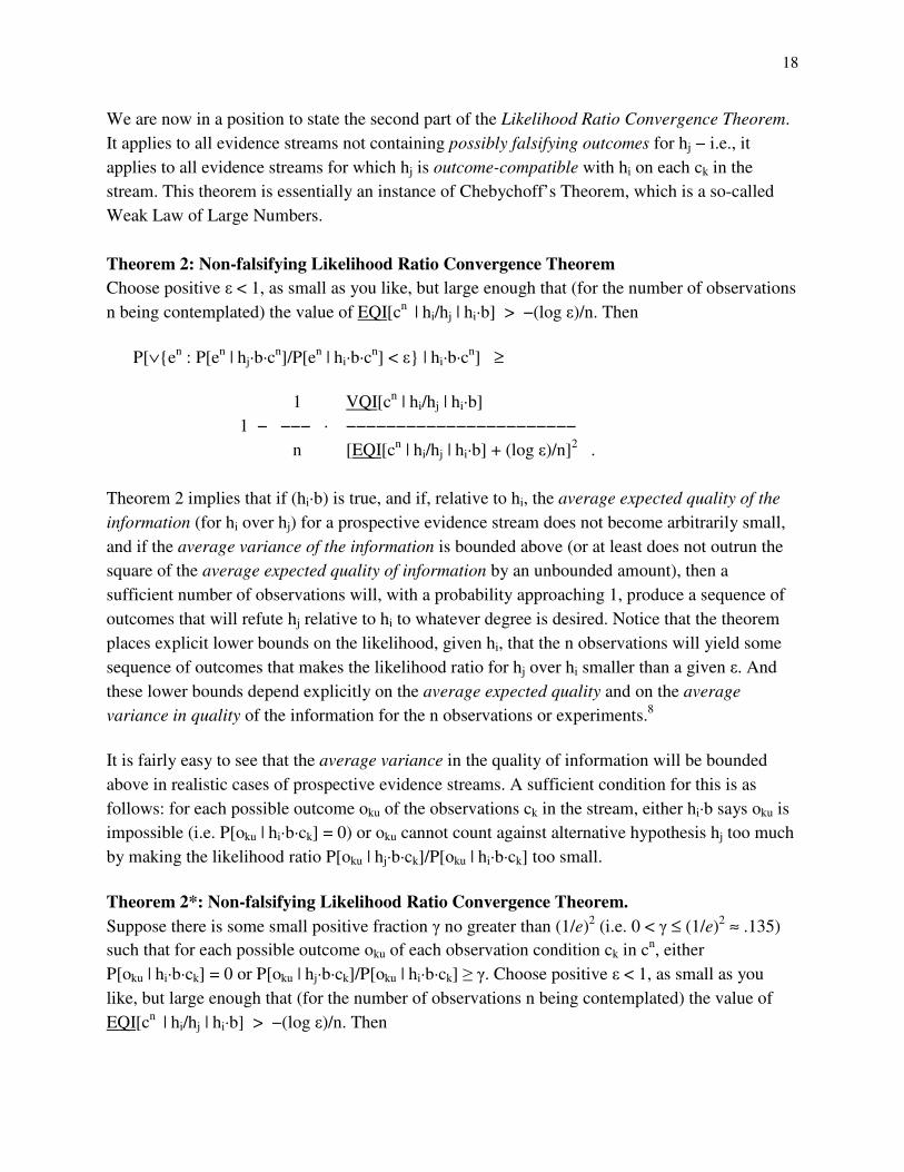
We are now in a position to state the second part of the Likelihood Ratio Convergence Theorem. It applies to all evidence streams not containing possibly falsifying outcomes for hj − i.e., it applies to all evidence streams for which hj is outcome-compatible with hi on each ck in the stream. This theorem is essentially an instance of Chebychoff’s Theorem, which is a so-called Weak Law of Large Numbers. Theorem 2: Non-falsifying Likelihood Ratio Convergence Theorem Choose positive � < 1, as small as you like, but large enough that (for the number of observations n being contemplated) the value of EQI[cn | hi/hj | hi·b] > −(log �)/n. Then

P[∨{en : P[en | hj·b·cn]/P[en | hi·b·cn] < �} | hi·b·cn] ≥

1 VQI[cn | hi/hj | hi·b] 1 − −−− · −−−−−−−−−−−−−−−−−−−−−−− n [EQI[cn | hi/hj | hi·b] + (log �)/n]2 . Theorem 2 implies that if (hi·b) is true, and if, relative to hi, the average expected quality of the information (for hi over hj) for a prospective evidence stream does not become arbitrarily small, and if the average variance of the information is bounded above (or at least does not outrun the square of the average expected quality of information by an unbounded amount), then a sufficient number of observations will, with a probability approaching 1, produce a sequence of outcomes that will refute hj relative to hi to whatever degree is desired. Notice that the theorem places explicit lower bounds on the likelihood, given hi, that the n observations will yield some sequence of outcomes that makes the likelihood ratio for hj over hi smaller than a given �. And these lower bounds depend explicitly on the average expected quality and on the average variance in quality of the information for the n observations or experiments.8

It is fairly easy to see that the average variance in the quality of information will be bounded above in realistic cases of prospective evidence streams. A sufficient condition for this is as follows: for each possible outcome oku of the observations ck in the stream, either hi·b says oku is impossible (i.e. P[oku | hi·b·ck] = 0) or oku cannot count against alternative hypothesis hj too much by making the likelihood ratio P[oku | hj·b·ck]/P[oku | hi·b·ck] too small.

Theorem 2*: Non-falsifying Likelihood Ratio Convergence Theorem. Suppose there is some small positive fraction � no greater than (1/e)2 (i.e. 0 < � ≤ (1/e)2 ≈ .135) such that for each possible outcome oku of each observation condition ck in cn, either P[oku | hi·b·ck] = 0 or P[oku | hj·b·ck]/P[oku | hi·b·ck] �. Choose positive � < 1, as small as you like, but large enough that (for the number of observations n being contemplated) the value of EQI[cn | hi/hj | hi·b] > −(log �)/n. Then

19

P[∨{en : P[en | hj·b·cn]/P[en | hi·b·cn] < �} | hi·b·cn] >

1 (log �)2 1 − −−− · −−−−−−−−−−−−−−−−−−−−−−− n [EQI[cn | hi/hj | hi·b] + (log �)/n]2 .

Notice, the antecedent condition of the theorem, that “either P[oku | hi·b·ck] = 0 or P[oku | hj·b·ck]/P[oku | hi·b·ck] �, for some small positive � ≤ (1/e)2”, does not in any way favor hypothesis hi. The condition only rules out the possibility that some outcomes might furnish extremely strong evidence against hj relative to hi. (This condition is only needed because our measure of evidential distinguishability, QI, blows up whenever the ratio P[oku | hj·b·ck]/P[oku | hi·b·ck] is becomes extremely small.) Furthermore, this condition is really no restriction at all on possible experiments or observations. If ck has some possible outcome-sentence oku that would make P[oku | hj·b·ck]/P[oku | hi·b·ck] < � (for a given small � of interest), one may disjunctively lump oku together with some other outcome-sentence okv for observation ck. Then, the antecedent condition of the theorem will be satisfied, but with the sentence ‘(oku∨okv)’ treated as a single outcome (e.g., in the formula for EQI and for VQI). It can be proved that the only effect of such “disjunctive lumping” on the quality of the information for ck is to make EQI a bit smaller than it would otherwise be.

The point of the Convergence Theorems presented here is to assure us, in advance of the consideration of any specific pair of hypotheses, that if the possible evidence streams that test them have certain characteristics which reflect the evidential distinguishability of the hypotheses, then it is highly likely that outcomes yielding small likelihood ratios will result. And these theorems provide finite lower bounds on how quickly convergence is likely to occur, bounds that show one need not wait through some infinite long run for convergence to occur. Indeed, for any evidence sequence in which the probability distributions are at all well behaved, the actual likelihood of obtaining outcomes that yield small likelihood ratio values will inevitably be much higher, much closer to 1, than the lower bounds given by Theorems 1 and 2. 9

Thus, the theorem provides a lower bound on the likelihood of obtaining small likelihood ratios. It shows that the larger the value of EQI for an evidence stream, the more likely that stream is to produce a sequence of outcomes that yield very small likelihood ratios. But even if EQI remains quite small, a long enough stream, n, will almost surely produce an outcome sequence having a very small likelihood ratio.

In sum, according to Theorems 1 and 2, each hypothesis hi says, via likelihoods, that given enough observations, it will very likely dominate its empirically distinct rivals in a contest of likelihood ratios. And even a sequence of observations with an extremely low average expected quality of information is very likely to do the job if that sequence is long enough. Presumably,

20

the true hypothesis speaks truthfully about this, and its competitors lie. Thus (by Equation 1), as evidence accumulates, the degree of support for false hypotheses will very probably approach 0, indicating that they are probably false; and as this happens, (by Equations 2 and 3) the degree of support for the true hypothesis will approach 1, indicating its probable truth.

3. Inductive Support When the Likelihoods are Mushy

Objective likelihoods are highly desirable. For, to the extent that members of a scientific community disagree on the values of likelihoods, they disagree about the empirical content of their hypotheses − they disagree on what the hypothesis says about what the world is likely to be like. As a result, agents may well end up disagreeing about which hypotheses become refuted or supported by the very same stream of evidence. To the extent that this can happen, the empirical import of such hypotheses may be just too vague or mushy for anything like objective tests against rivals.

However, the values of likelihoods themselves are not the most crucial factors in the way evidence impacts hypotheses. Rather (as Equations 1-3 show), it is ratios of likelihoods that do the heavy lifting. So, if two support functions P� and P� disagree on the values of likelihoods, they may, nevertheless, largely agree on the refutation or support that accrues to various rival hypotheses hi and hj, if the evidence on which the hypotheses are evaluated satisfies the following condition:

Directional Agreement Condition: For each experiment or observation c and each of its possible outcomes o, the likelihood ratios agree in direction to the extent that whenever the ratio is greater than 1 for one of the support functions, it is also greater than 1 for the other; and whenever it is less than 1 for one of them, it is also less than 1 for the other: i.e., P�[o | hj·b·c]/P�[o | hi·b·c] > 1 iff P�[o | hj·b·c]/P �[o | hi·b·c] > 1, and P�[o | hj·b·c]/P �[o | hi·b·c] < 1 iff P�[o | hj·b·c]/P �[o | hi·b·c] < 1.

In that case the evidence will support hi over hj according to P� just in case it does so for P� as well, although the strength of support may differ between them. And although the rate at which cumulative likelihood ratios increase or decrease may differ for the two such support functions, the stream of evidence should affect their refutation or support in much the same way.

Now, it happens that the Likelihood Ratio Convergence Theorems (1 and 2) do not rely in any essential way on the assumption that likelihoods are objective or have intersubjectively agreed values − i.e., the proofs of these theorems do not rely on this. Rather, these theorems may be applied to each support function P� individually. So, if in some contexts the likelihoods fail to be objective or to have agreed values within scientific community, these theorems nevertheless continue to hold for each support function individually.

21

When the Directional Agreement Condition is satisfied, the application of Theorems 1 and 2 to each support function separately shows that a significant amount of evidence will almost surely bring each support function in Vagueness and Diversity classes to agreement on very small likelihood ratios against false competitors of a true hypothesis. And when that happens, the evidence will bring all of these support functions into agreement regarding the strong refutation (near 0 posterior probability) of the false rivals. And this will push the posterior probability of the true hypothesis towards 1.10

Even if there are a few controversial likelihood ratios (where P� says the ratio is somewhat greater than 1, while and P� assigns a value somewhat less than 1) these may not greatly effect the trend of P� and P� towards agreement on the refutation and support of hypotheses on the whole evidence stream, provided that the controversial ratios are not so extreme as to overwhelm the stream of other evidence on which the likelihood ratios directionally agree. So, provided there is rough agreement on the empirical import of hypotheses (as expressed by likelihood ratios) among the support functions in Vagueness and Diversity sets that represent the range of views among members of the scientific community, and provided enough quality experiments or observations can be performed, the community will almost surely come to agree on the refutation of the empirically distinct, false competitors of the true hypothesis, and the true hypothesis will tend to rise to the top of the heap. Of course, if the true hypothesis has empirically equivalent rivals, they will rise along with it. We may only be assured that its disjunction with empirically equivalent rivals will be driven to 1 as evidence lays the empirically distinct alternatives low. The true hypothesis will itself approach 1only if its empirically equivalent rivals are laid low as well, by non-evidential prior plausibility considerations.

Notes

1 The present paper owes an enormous debt to Clark Glymour’s incisive critique of Bayesian confirmation theory, “Why I am not a Bayesian”, from his book Theory and Evidence. Although I do not directly discuss Glymour’s paper here, those of you familiar with it will recognize the extent to which the present paper is motivated by an attempt to respond to the challenges for the Bayesian approach raised by Glymour’s paper.

2 ‘All emeralds are green (at all times)’ has the same syntactic structure as ‘All emeralds are grue (at all times)’. So, if syntactic structure determines priors, then these hypotheses should have the same priors. Indeed, both should have prior probabilities approaching 0. For, there are an infinite number of competitors of these two hypotheses, each sharing the same syntactic structure:

22

consider the hypotheses ‘All emeralds are gruen (at all times)’, where to be gruen at a given time is just to be green at that time if prior to midnight n days from January 1, 2010, and to be blue at that time if after midnight n days from that date. A purely syntactic specification of the priors should assign all of these hypotheses the same prior probability. But these are mutually exclusive hypotheses; so their prior probabilities must sum to a value no greater than 1. And the only way this can happen is for ‘All emeralds are green’ and each of its gruen competitors to have prior probability values equal to 0 (or infinitesimally close to 0).

3 When, for example, a new desease is discovered, a new hypothesis hu+1 about possible causes of patients’ symptoms is made explicit. The old catch-all was, “the symptoms are caused by some unknown desease − some desease other than h1,…, hu”. So the new catch-all hypothesis must now state that “the symptoms are caused by one of the remaining unknown deseases − some desease other than h1,…, hu, hu+1”. And, clearly, P�[hK | b] = P�[~h1·…·~hu | b] = P�[~h1·…·~hu· (hu+1 ∨ ~hu+1) | b] = P�[~h1·…·~hu·~hu+1 | b] + P�[hu+1 | b] = P�[hK* | b] + P�[hu+1 | b]. Thus, the new hypothesis hu+1 is “peeled off” of the old catch-all hypothesis K, leaving a new catch-all hypothesis K* with a prior probability value equal to that of the old catch-all minus the prior of the new hypothesis: P�[hK* | b] = P�[hK | b] − P�[hu+1 | b].

4 This claim depends, of course, on hi being empirically distinct from each alternative hj. I.e., there must be conditions ck with possible outcomes oku on which the likelihoods differ: P[oku | hi·b·ck] ≠ P[oku | hj·b·ck]. Otherwise hi and hj are empirically equivalent, and no amount of evidence can support one over the other. Did you think a confirmation theory could possibly do better? − could use evidence to confirm the true hypothesis over empirically equivalent rivals? If the true hypothesis has empirically equivalent rivals, then convergence just implies that the odds against the disjunction of the true hypothesis with these rivals very probably goes to 0, and so the posterior probability of this disjunction goes to 1. Among empirically equivalent hypotheses the ratio of their posterior probabilities must equal the ratio of their priors: P�[hj | b·cn·e n] / P�[hi | b·cn·e n] = P�[hj | b] / P�[hi | b]. So the true hypothesis will have a posterior probability near 1 (after evidence drives the posteriors of empirically distinguishable rivals near 0) just in case non-evidential considerations make its evidence-independent plausibility much higher than the sum of the plausibility ratings of the empirically equivalent rivals.

5 It seems to me that the Bayesian probability functions employed in confirmation theory, which I call inductive support functions, must be distinct from subjectivist or personalist degree-of-belief functions. This is a good place to briefly discuss a reason for thinking so. The idea is that although likelihoods have a high degree of objectivity in many scientific contexts, it is difficult for realistic belief functions, even ideal realistic belief functions, to properly represent the objectivity of the likelihoods. This is an aspect of the so-called problem of old evidence.

23

Belief functions are supposed to provide an ideal model of belief strengths for agents. They extend the notion of ideally consistent belief to a probabilistic notion of ideally coherent belief strengths for an agent. There is no harm in such idealization. It is supposed to provide a normative guide to decision making. An agent is supposed to make decisions based on her belief-strengths about the state of the world, her belief strengths about possible consequences of actions, and her assessment of the utility (i.e. desirability) of these consequences. But the very role that belief strengths are supposed to play in decision making makes them ill-suited for inductive inferences in the sciences, where the likelihoods are often supposed to be objective values, or at least inter-subjectively agreed values, that represent the empirical import of hypotheses. For the purposes of decision making, degree-of-belief functions should represent the agent's belief strengths based on everything she presently knows. So, degree-of-belief likelihoods must represent how strongly the agent would believe the evidence if the hypothesis were added to everything else she presently knows. Here they differ from support-function likelihoods, which are supposed to represent what the hypothesis (together with explicit background and experimental conditions) says or implies about the evidence, not the belief strength in the evidence when the hypothesis is added to everything else the agent knows. As a result, degree-of-belief likelihoods are saddled with the problem of old evidence – a problem not shared by support function likelihoods. And it turns out that the old evidence problem for likelihoods is much worse than is usually recognized.

Here is the problem. If the agent is already certain of an evidence statement e, then her belief-function likelihoods for that statement must be 1, on every hypothesis. I.e., if Q� is her belief function and Q�[e] = 1, then it follows from the axioms of probability theory that Q�[e | hi·b·c] = 1 for every hypothesis hi, even hypotheses that would seem, themselves, to imply that e is quite unlikely (given b·c). But the problem goes even deeper. It not only applies to evidence that the agent knows with certainty. It turns out that almost anything the agent learns that changes how strongly she believe e will influence the value of her belief-function likelihood for e, because Q�[e | hi·b·c] represents the agent's belief strength given everything she knows.

To see how the problem extends to less-than-certain evidence, consider the following example. (I’ll supress the b and c here, as subjectivist Bayesians often do, since they will make no difference for present purposes.) A physician intends to test her patient for heart disease, h, with a treadmill test. She knows from medical studies that there is a 10% false negative rate for this test; so her belief-strength for a negative result, e, given heart disease is present is Q�[e | h] = .10. Now, her nurse is very professional and is usually unaffected by patients’ test results. So, if asked, the physician would say her belief strength that her nurse will be devastated, d, if the test is positive (i.e. if ~e) is around Q�[d | ~e] = .05. And let us suppose, as seems reasonable, that this belief-strength is independent of whether h is in fact true − i.e. Q�[d | ~e·h] = Q�[d | ~e]. The

24

nurse then says to the physician, in a completely convincing way, “if his test comes out positive, I’ll be devastated.” The physician’s new belief function likelihood for a false negative must then become Q�-new[e | h] = Q�[e | h·(~e ⊃d)] = .69 (since Q�[e | h·(~e ⊃d)] = Q�[~e ⊃d | h·e] · Q�[e | h] / (Q�[~e ⊃d | h·e] · Q�[e | h] + Q�[~e ⊃d | h·~e] · Q�[~e | h]) = Q�[e | h] / (Q�[e | h] + Q�[d | ~e·h] · Q�[~e | h]) = .1/(.1 + (.05)(.9)) >.69).

The point is that even the most trivial knowledge of conditional (or disjunctive) claims involving e may completely upset the value of the likelihood for an agent’s belief function. And an agent will almost always have some such trivial knowledge. E.g., the physician in the previous example may also learn that if the treadmill test is negative for heart disease, then, (1) the patient's worried mother will be relieved, (2) the patient's insurance company won't cover additional tests, (3) it will be the thirty-seventh negative treadmill test result she has received for a patient this year,…, etc. Updating on such conditionals can force physicians’ belief functions to deviate widely from the evidentially relevant objective, textbook values of test result likelihoods.

More generally, it can be shown that the updating of the agent’s belief function on almost any kind of evidence for or against the truth of a prospective evidence claim e, even uncertain evidence for e, as may come through Jeffrey updating, completely undermines the objective or inter-subjectively agreed likelihoods that a belief function might have expressed before updating. This should be no surprise. The agent's belief function likelihoods reflect her total degree-of-belief in e, based on h together with everything else she knows about e. So the agent's present belief function may capture appropriate, public likelihoods for e only if e is completely isolated from the agent's other beliefs. And this will rarely be the case.

The following theorem shows how the problem of old evidence arises for uncertain evidence when Jeffrey updating applies. (I again suppress ‘b’ and ‘c’ here.)

Theorem: Suppose that some new datum changes the agent’s degree-of-belief function from Q�-old to Q�-new by updating her belief strengths in “uncertain evidence” statements for the possible evidential outcomes {o1, ..., ou}. (Such updating implies that Q�-new[oi] ≠ Q�−old[oi] for at least one of the oi.) And suppose that one of the following two conditions hold: (1) at least one of the alternative hypotheses hi assigns a non-zero likelihood to each alternative outcome ok of the experiment – i.e., there is an hi such that for all ok, Q�-old[ok | hi] > 0; or (2) at least one possible alternative outcome gets a non-zero likelihood from each hypothesis – i.e., there is an ok such that for all hi, Q�-old[ok | hi] > 0. And suppose the belief strengths for each of the alternative hypotheses hi on the various ok are maintained through this belief function update (as in Jeffrey updating) − i.e., Q�-new[hk | oi] = Q�-old[hk | oi] for each hk and oi. Then some of the likelihoods for the new belief

25

function Q�-new[oi | hk] must differ from the corresponding old belief function likelihoods Q�-old[oi | hk].

One Bayesian subjectivist response to the old evidence problem is that the belief functions employed in scientific inductive inferences should often be “counterfactual” belief functions, which represent what the agent would have believed if known evidence e were subtracted (in some suitable way) from everything else she knows (see, e.g. Howson & Urbach, 1993). However, our examples show that merely subtracting e won't do. One must also subtract any conditional statements containing e. And one must subtract any uncertain evidence for or against e as well. So the counterfactual belief function idea needs a lot of working out if it is to rescue the idea that the usually Bayesian degree-of-belief functions can provide a viable account of the likelihoods employed by the sciences in inductive inferences.

6 There is one kind of data that may violate Clause 2 of the Independent Evidence Assumption and that may not be easily handled by the chunking of locally depend data, as just described. That is, there may be cases where some small quantity of past data ties down the numerical values of some free parameters in a hypothesis, parameters that are relevant to the outcomes of the other experiments − e.g., parameters representing values of some constants of nature. For our purposes the relevance of such parameter fixing data may be handled in either of two ways. It may be made part of the background information b. Alternatively, a hypothesis with free parameters may be viewed as a disjunction of hypotheses, each containing specific values for the parameters. Evidence that “fills in the values” is just evidence that falsifies those alternative hypotheses that specify incorrect parameter values. Then, Clause 2 should be satisfied by each of the alternative filled-in hypothesis, which themselves make specific claims about the parameter values. Either way, dependence will then remain localized, and Clause 2 is easily satisfied by chunking all remaining inter-dependent bits of evidence into independent units. 7 Technically, suppose that partition Ok can be further “subdivided” into more outcome-descriptions by replacing okv with two “parts”, okv

* and okv#, to produce a new outcome space

Ok* = {ok1, …, okv

*, okv#, …, okw}, (where P[okv

* · okv# | hi·b·cn] = 0, P[okv

* | hi·b·cn] + P[okv

# | hi·b·cn] = P[okv | hi·b·cn], and similarly for hj). Then the new EQI* (based on Ok*) is greater than or equal to EQI (based on Ok); and EQI* > EQI just in case at least one of the new likelihood ratios, e.g., P[okv

* | hi·b·cn] / P[okv* | hj·b·cn], differs in value from the “undivided”

outcome’s likelihood ratio, P[okv | hi·b·cn] / P[okv | hi·b·cn].

8 It should now be clear why the boundedness of EQI above 0 is important. Theorem 2 applies only when EQI[cn | hi/hj | hi·b] > −(log �)/n. But this requirement is not a strong assumption. For, the Boundedness of EQI Theorem shows that the empirical distinctness of two hypotheses

26

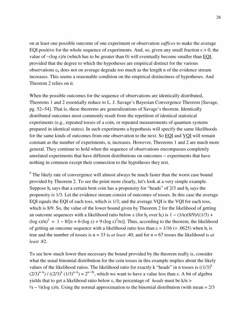
on at least one possible outcome of one experiment or observation suffices to make the average EQI positive for the whole sequence of experiments. And, so, given any small fraction � > 0, the value of −(log �)/n (which has to be greater than 0) will eventually become smaller than EQI, provided that the degree to which the hypotheses are empirical distinct for the various observations ck does not on average degrade too much as the length n of the evidence stream increases. This seems a reasonable condition on the empirical distinctness of hypotheses. And Theorem 2 relies on it.

When the possible outcomes for the sequence of observations are identically distributed, Theorems 1 and 2 essentially reduce to L. J. Savage’s Bayesian Convergence Theorem [Savage, pg. 52−54]. That is, these theorems are generalizations of Savage’s theorem. Identically distributed outcomes most commonly result from the repetition of identical statistical experiments (e.g., repeated tosses of a coin, or repeated measurements of quantum systems prepared in identical states). In such experiments a hypothesis will specify the same likelihoods for the same kinds of outcomes from one observation to the next. So EQI and VQI will remain constant as the number of experiments, n, increases. However, Theorems 1 and 2 are much more general. They continue to hold when the sequence of observations encompasses completely unrelated experiments that have different distributions on outcomes − experiments that have nothing in common except their connection to the hypotheses they test.

9 The likely rate of convergence will almost always be much faster than the worst case bound provided by Theorem 2. To see the point more clearly, let's look at a very simple example. Suppose hi says that a certain bent coin has a propensity for “heads” of 2/3 and hj says the propensity is 1/3. Let the evidence stream consist of outcomes of tosses. In this case the average EQI equals the EQI of each toss, which is 1/3; and the average VQI is the VQI for each toss, which is 8/9. So, the value of the lower bound given by Theorem 2 for the likelihood of getting an outcome sequences with a likelihood ratio below � (for hj over hi) is 1 − (1/n)(8/9)/((1/3) + (log �)/n)2 = 1 − 8/[n + 6·(log �) + 9·(log �)2/n)]. Thus, according to the theorem, the likelihood of getting an outcome sequence with a likelihood ratio less than � = 1/16 (= .0625) when hi is true and the number of tosses is n = 33 is at least .40; and for n = 67 tosses the likelihood is at least .82.

To see how much lower then necessary the bound provided by the theorem really is, consider what the usual binomial distribution for the coin tosses in this example implies about the likely values of the likelihood ratios. The likelihood ratio for exactly k “heads” in n tosses is ((1/3)k (2/3)n−k) / ((2/3)k (1/3)n−k) = 2n−2k, which we want to have a value less than �. A bit of algebra yields that to get a likelihood ratio below �, the percentage of heads must be k/n > ½ − ½(log �)/n. Using the normal approximation to the binomial distribution (with mean = 2/3

27

and variance = (2/3)·(1/3)/n) the actual likelihood of obtaining an outcome sequence having a likelihood ratio less than � is given by �[(mean − (½ − ½(log �)/n))/(variance)½] = �[((n + 6·(log �) + 9·(log �)2/n)/8)½] (where �[x] gives the value of the standard normal distribution from −� to x). Now let � = 1/16 (= .0625), as before. So the actual likelihood of obtaining a stream of outcomes with likelihood ratio this small when hi is true and the number of tosses is n = 33 is �[1.29] ≈ .90, whereas we saw that the lower bound given by Theorem 2 was .40. And if the number of tosses in increased to n = 67, the likelihood of obtaining an outcome sequence with a likelihood ratio this small (i.e., � = 1/16) is �[2.38] ≈ .99, whereas the lower bound from Theorem 2 for this likelihood is 82. Indeed, to actually get a likelihood of .82 that the evidence stream will produce a likelihood ratio less than � = .0625, the number of tosses needed is only n = 25. (Note: In these examples we’ve used “identically distributed” trials − repeated tosses of a coin − as an illustration. But Theorem 2 applies much more generally; it applies to any evidence sequence, no matter how diverse the probability distributions for the various experiments or observations in the sequence.)

10 In many scientific contexts this is the best we can hope for. But it still provides a very reasonable representation of inductive support. Let’s consider, for example, the hypothesis that the land masses of Africa and South America separated and drifted apart over the eons, the drift hypothesis, as opposed to the hypothesis that the continents have fixed positions that they acquired when the earth first formed and contracted and cooled, the contractionist hypothesis. One may not be able to determine anything like precise likelihoods that, on each hypothesis, the shape of the east coast of South America should match the shape of the west coast of Africa as closely as it in fact does, or that the geology of the two coasts should match up so well, or that the plant and animal species on these distant continents should be as similar as they are. But experts may readily agree that each of these observations is much more likely on the drift hypothesis than on the contractionist hypothesis. And jointly these observations should constitute very strong evidence for drift over contraction.

Historically, the case of continental drift is more complicated. Geologists tended to largely dismiss this evidence until the 1960s. This was not because the evidence wasn't strong in its own right. Rather, this evidence was found unconvincing because it was not sufficient to overcome (prior) plausibility considerations that made the drift hypothesis seem extremely implausible — much less plausible that the contraction hypothesis. The problem was that there seemed to be no plausible mechanism through which drift might occur. It was argued, quite plausibly, that no known force could push or pull the continents apart, and that the less dense continental material could not push through the denser material that makes up the ocean floor. These plausibility objections were overcome when a plausible mechanism was articulated — i.e. the continental crust floats atop molten material and moves apart as convection currents in the molten material

28

carry it along. The case was pretty well clinched when evidence for this mechanism was found in the form of “spreading zones” containing alternating strips of magnetized material at regular distances from mid-ocean ridges. The magnetic alignments of materials in these strips corresponds closely to the magnetic alignments found in magnetic materials in dateable sedimentry layers at other location on the earth. These magnetic alignments indicate time periods when the direction of earth’s magnetic field has reversed. And this gave geologists a way of measuring the rate at which the sea floor spreads and the continents are moved apart. Although geologists may not be able to determine anything like precise values for the likelihoods of this any of this evidence on each of the alternative hypotheses, the evidence is universally agreed to be much more likely on the drift hypothesis than on the contractionist alternative. (And, with the emergence of a plausible mechanism, the drift hypothesis seems not so overwhelmingly implausible prior to the evidence, either.) So, the value of a likelihood ratio may be objective or public enough, even when precise values for individual likelihoods are not available.