The Sovereign-Bank Interaction in the EurozoneCrisis

Maximilian Goedl∗

University of Graz

October 2, 2017

Abstract

This paper investigates the relationship between government debt default, the bank-ing sector and the wider economy. It builds a model of the public bond market, thebanking sector and the real economy to study the mechanism by which a governmentdefault affects the other sectors and shows that this model can explain some “stylizedfacts” of the Eurozone crisis. The key aspect of the model is a friction in the financialmarket which forces banks to hold part of their assets in the form of government bonds.In such a model, an exogenous increase in the probability of default can lead to the jointoccurrence of a credit crunch (i.e. declining bank lending and rising spreads betweenloan interest rates and deposit rates) and a decline in output. The paper also shows thatan adverse technology shock (an exogenous decline in total factor productivity) cannotfully explain these phenomena.

Keywords: Government default, financial frictions, business cycle model.

JEL Codes E37, E44, H63.

∗I would like to thank the Graf Hardegg’sche Stiftung for financial support as well as Paul de Grauwe, JoernKleinert, Karl Farmer, Christoph Zwick, Isabel Hanisch, and Jens Boysen-Hogrefe for valuable comments anddiscussions.

1

1 Introduction

The recent economic crisis in the Eurozone had three elements.1 One the one hand, therewas a financial crises in which asset prices plunged, credit spreads widened, financial firmswent bankrupt, and the inter-bank market froze up. Second, there was a government debtcrisis in some Eurozone countries where interest spreads spiked suddenly and unexpectedlyand forced governments to seek fiscal support from other countries and international organi-zations. Third, there was a deep and long downturn in the real economy producing recordhighs of unemployment in some member countries.

Although a large literature has developed attempting to explain each element of the crisisin isolation, few attempts have been made to provide a coherent framework for analyzing allthree elements of the crisis and their interaction. The goal of this paper is to provide such aframework. First, it develops a fully-specified general equilibrium model which can explainthe joint occurrence of a credit crunch, a government debt crisis and a decline in economicactivity. Second, it shows that a calibrated version of the model can replicate some basicquantitative features of the Eurozone crisis.

In building this model, we draw on two strands of literature. We borrow from the workof Gertler and Kiyotaki (2010) among others who integrate financial intermediaries (i.e. abanking sector) into a business cycle model. This literature posits that financial intermedia-tion is subject to problems of asymmetric information and limited commitment which giverise to an endogenous constraint on the lending activity of banks. This financial friction actsto amplify the impact of exogenous disturbances (“shocks”) to the real economy. Moreover,the financial sector can also be a source of shocks in these models.

The second input for the model comes from the literature on quantitative models ofsovereign debt crises. In recent work by Gennaioli et al. (2014) and Sosa-Padilla (2012),banks hold government debt securities on their balance sheets which exposes them to therisk of government default. If the government defaults, financial sector incurs losses on theirgovernment bonds which reduces their ability to lend to firms and thus affects and the realeconomy.

Previous studies have proposed a number of causal mechanisms for the government-bankinteraction observed in the Eurozone crisis. Acharya et al. (2014) build a model in whichbank bailouts by governments produce a negative effect on public finances which, in turn,reduce the value of the implicit government guarantees for bank debt. They provide empiricalevidence for their model by showing that the announcement of bank bailouts was associated

1Shambaugh (2012) provides a concise overview of the Eurozone crisis.

2

with increasing sovereign CDS spreads and that sovereign and bank CDS tended to move insync after the bailouts. Bolton and Jeanne (2011) provide a detailed theoretical analysis ofcontagious sovereign defaults in which bank balance sheets play a crucial role. They focuson the incentives of banks to diversify their bond portfolio as well as on the government’sincentives to default under different scenarios of financial and fiscal integration.

In a similar vein, Mody and Sandri (2012) show that, beginning with the nationalizationof Anglo Irish bank in 2009, sovereign interest spreads were positively correlated with a fi-nancial stress indicator. They interpret this finding in the context of a stylized model in whichthe government faces a trade-off between bailing out weak banks to support the economy andkeeping public debt at a sustainable level. Depending on initial levels of debt (among otherthings), the model predicts bank bailouts can lead to the vicious circle described above.De Bruyckere et al. (2013) investigate risk spillovers between bank and sovereign bonds inthe Eurozone using data from the EBA “stress test” and find that banks with a weak capitalbuffer, a weak funding structure and less traditional banking activities are particularly vul-nerable to risk spillovers. Their results further support the view that sovereign default riskand fragile financial institutions mutually reinforce each other.

Recent theoretical work by Gennaioli et al. (2014) shows that government defaults arecostly because they destroy the balance sheets of domestic banks, leading to declines inprivate credit and output losses. Using data from Italy, Bocola (2016) estimates a similarmodel concludes that an increase in default risk has contributed significantly to the observeddecline in output. Sosa-Padilla (2012) employs a similar framework to build a quantitativemodel of sovereign debt default. He found that his model can replicate some of the keyfeatures of the recent Argentine debt crisis.

This paper’s main contribution is to incorporate the government-bank interaction into anotherwise standard business cycle model to study the effect of an exogenous increase in theprobability of a government default, which we call a “government default shock”. It arguesthat such a shock can explain some stylized facts about the Eurozone crisis. It also showsthat a conventional (adverse) technology shock, i.e. an exogenous decrease in total factorproductivity, can explain some but not all of these stylized facts. This suggests that attemptsto explain the Eurozone crisis as the consequence of ”real shocks” faces serious empiricalchallenges. However, focusing only on the government interest spread and quantity vari-ables such as output, investment, consumption, bank lending and employment, one cannotdifferentiate empirically between technology and government default shocks. For that, it iscrucial to look at the behavior of bank interest rates. The model thus provides a basis for

3

further empirical research on the sources of the Eurozone crisis.The remainder of the paper is organized as follows. The next section establishes some

“stylized facts” about the Eurozone crisis. Section 3 presents and discusses the model. Sec-tion 4 deals with the calibration of the model. Section 5 shows the results of simulations ofthe calibrated model. Finally, section 6 sums up the main results of the analysis and discussesavenues for future research.

2 The Eurozone crisis: some stylized facts

In this section, we document a set of stylized facts that our model aims to explain. Ourfocus is on five member states of the Eurozone that have experienced a government debtcrisis: Greece, Italy, Ireland, Spain, and Portugal. The data for this section come from theEuropean Central Bank’s database unless otherwise indicated. The four stylized facts wewish to establish are:

1. Government interest spreads increased after 2010, then declined beginning in 2012;

2. Banks’ lending margins (lending-borrowing spreads) increased after 2010, but with atime lag compared to government spreads;

3. Banks’ lending volumes (loans to non-financial businesses) decreased after 2010;

4. Economic activity decreased after 2010 and only slowly recovered beginning in 2013.

2.1 Government interest spreads

The government interest spread is defined as the difference between the yield on (long-term)government bonds and the risk-free interest rate. It can be interpreted as a market-basedmeasure of the perceived risk of a government default insofar as a the larger spread impliesa higher (perceived) default probability.2 In most of the existing literature, the risk-freerate is taken to be the yield of German government bonds, presumably because the Germangovernment is supposed to be the “safest” within the eurozone. We depart from this practiceand use the interest rate on bank deposits as a proxy of the risk-free rate, since bank depositsin the Eurozone are protected by deposit insurance and can thus be expected to carry no riskpremium. This choice is not critical however, because the German interest rate moves in

2Risk is not the only reason for interest spreads. Differences in liquidity as well as collateral value also playrole.

4

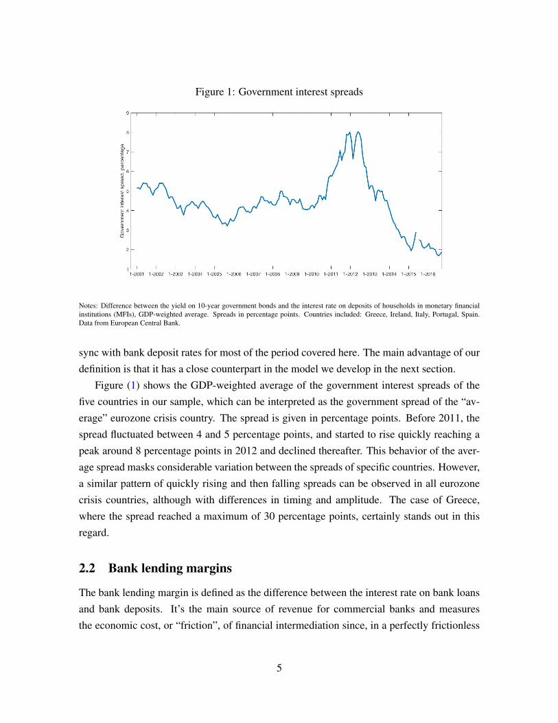
Figure 1: Government interest spreads

Notes: Difference between the yield on 10-year government bonds and the interest rate on deposits of households in monetary financialinstitutions (MFIs), GDP-weighted average. Spreads in percentage points. Countries included: Greece, Ireland, Italy, Portugal, Spain.Data from European Central Bank.

sync with bank deposit rates for most of the period covered here. The main advantage of ourdefinition is that it has a close counterpart in the model we develop in the next section.

Figure (1) shows the GDP-weighted average of the government interest spreads of thefive countries in our sample, which can be interpreted as the government spread of the “av-erage” eurozone crisis country. The spread is given in percentage points. Before 2011, thespread fluctuated between 4 and 5 percentage points, and started to rise quickly reaching apeak around 8 percentage points in 2012 and declined thereafter. This behavior of the aver-age spread masks considerable variation between the spreads of specific countries. However,a similar pattern of quickly rising and then falling spreads can be observed in all eurozonecrisis countries, although with differences in timing and amplitude. The case of Greece,where the spread reached a maximum of 30 percentage points, certainly stands out in thisregard.

2.2 Bank lending margins

The bank lending margin is defined as the difference between the interest rate on bank loansand bank deposits. It’s the main source of revenue for commercial banks and measuresthe economic cost, or “friction”, of financial intermediation since, in a perfectly frictionless

5

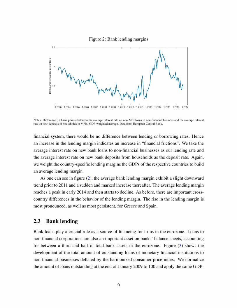
Figure 2: Bank lending margins

Notes: Difference (in basis points) between the average interest rate on new MFI loans to non-financial business and the average interestrate on new deposits of households in MFIs. GDP-weighted average. Data from European Central Bank.

financial system, there would be no difference between lending or borrowing rates. Hencean increase in the lending margin indicates an increase in “financial frictions”. We take theaverage interest rate on new bank loans to non-financial businesses as our lending rate andthe average interest rate on new bank deposits from households as the deposit rate. Again,we weight the country-specific lending margins the GDPs of the respective countries to buildan average lending margin.

As one can see in figure (2), the average bank lending margin exhibit a slight downwardtrend prior to 2011 and a sudden and marked increase thereafter. The average lending marginreaches a peak in early 2014 and then starts to decline. As before, there are important cross-country differences in the behavior of the lending margin. The rise in the lending margin ismost pronounced, as well as most persistent, for Greece and Spain.

2.3 Bank lending

Bank loans play a crucial role as a source of financing for firms in the eurozone. Loans tonon-financial corporations are also an important asset on banks’ balance sheets, accountingfor between a third and half of total bank assets in the eurozone. Figure (3) shows thedevelopment of the total amount of outstanding loans of monetary financial institutions tonon-financial businesses deflated by the harmonized consumer price index. We normalizethe amount of loans outstanding at the end of January 2009 to 100 and apply the same GDP-

6

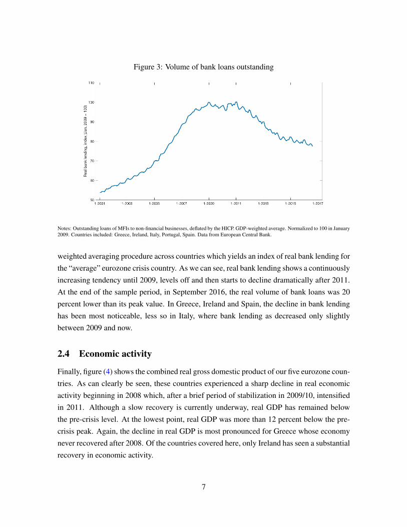
Figure 3: Volume of bank loans outstanding

Notes: Outstanding loans of MFIs to non-financial businesses, deflated by the HICP. GDP-weighted average. Normalized to 100 in January2009. Countries included: Greece, Ireland, Italy, Portugal, Spain. Data from European Central Bank.

weighted averaging procedure across countries which yields an index of real bank lending forthe “average” eurozone crisis country. As we can see, real bank lending shows a continuouslyincreasing tendency until 2009, levels off and then starts to decline dramatically after 2011.At the end of the sample period, in September 2016, the real volume of bank loans was 20percent lower than its peak value. In Greece, Ireland and Spain, the decline in bank lendinghas been most noticeable, less so in Italy, where bank lending as decreased only slightlybetween 2009 and now.

2.4 Economic activity

Finally, figure (4) shows the combined real gross domestic product of our five eurozone coun-tries. As can clearly be seen, these countries experienced a sharp decline in real economicactivity beginning in 2008 which, after a brief period of stabilization in 2009/10, intensifiedin 2011. Although a slow recovery is currently underway, real GDP has remained belowthe pre-crisis level. At the lowest point, real GDP was more than 12 percent below the pre-crisis peak. Again, the decline in real GDP is most pronounced for Greece whose economynever recovered after 2008. Of the countries covered here, only Ireland has seen a substantialrecovery in economic activity.

7

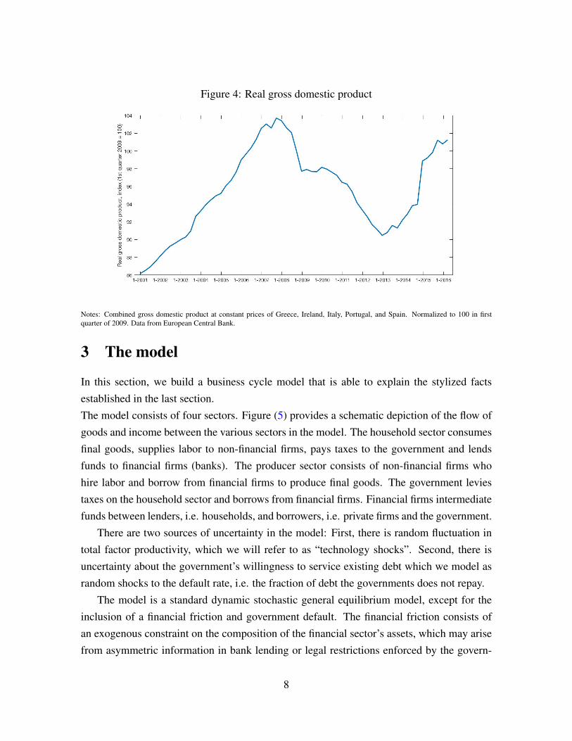
Figure 4: Real gross domestic product

Notes: Combined gross domestic product at constant prices of Greece, Ireland, Italy, Portugal, and Spain. Normalized to 100 in firstquarter of 2009. Data from European Central Bank.

3 The model

In this section, we build a business cycle model that is able to explain the stylized factsestablished in the last section.The model consists of four sectors. Figure (5) provides a schematic depiction of the flow ofgoods and income between the various sectors in the model. The household sector consumesfinal goods, supplies labor to non-financial firms, pays taxes to the government and lendsfunds to financial firms (banks). The producer sector consists of non-financial firms whohire labor and borrow from financial firms to produce final goods. The government leviestaxes on the household sector and borrows from financial firms. Financial firms intermediatefunds between lenders, i.e. households, and borrowers, i.e. private firms and the government.

There are two sources of uncertainty in the model: First, there is random fluctuation intotal factor productivity, which we will refer to as “technology shocks”. Second, there isuncertainty about the government’s willingness to service existing debt which we model asrandom shocks to the default rate, i.e. the fraction of debt the governments does not repay.

The model is a standard dynamic stochastic general equilibrium model, except for theinclusion of a financial friction and government default. The financial friction consists ofan exogenous constraint on the composition of the financial sector’s assets, which may arisefrom asymmetric information in bank lending or legal restrictions enforced by the govern-

8

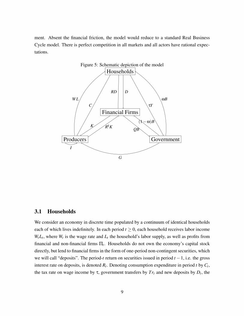
ment. Absent the financial friction, the model would reduce to a standard Real BusinessCycle model. There is perfect competition in all markets and all actors have rational expec-tations.

Figure 5: Schematic depiction of the model

Financial Firms

Households

GovernmentProducers

RD D

K RkK QB

(1−ω)B

τYωB

CWL

G

I

3.1 Households

We consider an economy in discrete time populated by a continuum of identical householdseach of which lives indefinitely. In each period t ≥ 0, each household receives labor incomeWtLt , where Wt is the wage rate and Lt the household’s labor supply, as well as profits fromfinancial and non-financial firms Πt . Households do not own the economy’s capital stockdirectly, but lend to financial firms in the form of one-period non-contingent securities, whichwe will call “deposits”. The period-t return on securities issued in period t−1, i.e. the grossinterest rate on deposits, is denoted Rt . Denoting consumption expenditure in period t by Ct ,the tax rate on wage income by τ, government transfers by Trt and new deposits by Dt , the

9

household’s budget constraint is given by

Ct +Dt =WtLt(1− τ)+Πt−Trt +RtDt−1. (1)

Note that all price variables are measured in units of the consumption good, which is innocu-ous since there are no nominal frictions in our model such that purely nominal changes haveno effect on real variables.Households period-t utility Ut = U(Ct ,Lt) is increasing in consumption and decreasing inlabor and fulfills the usual concavity conditions. Expected lifetime utility is given by

Et

∞

∑s=0

βsU(Ct+s,Lt+s), (2)

where β ∈ (0,1) is the pure time discount factor and Et denotes the expected value condi-tional on information available in period t. The household’s optimization problem consistsin choosing a sequence {(Ct+s,Lt+s,Dt+s)}∞

s=0 that maximizes lifetime utility (2) subject toa sequence of budget constraints such as (1).3

The first-order conditions for this optimization problem are

UC(Ct ,Lt) = λt , (3a)

−UL(Ct ,Lt) = λtWt(1− τ), (3b)

λt = Etβλt+1Rt+1, (3c)

for all t ≥ 0. Here UC denotes the marginal utility of consumption, UL the marginal disutilityof labor, and λt the marginal utility of real income, i.e. the Lagrange multiplier associatedwith the period-t budget constraint. In addition, there is a transversality condition

lims→∞

EtDt+s

Πsi=0Rt+i

= 0, (4)

which rules out endlessly growing deposits. For future reference, we define the stochasticdiscount factor

Λt,t+s ≡βλt+s

λt, (5)

3We leave out non-negativity conditions on Ct , Lt and Dt , because we will focus on equilibria in whichthese conditions are always fulfilled with strict inequality.

10

which represents the period-t value of receiving one unit of consumption in period t + s.For our numerical simulations, we will impose the following functional form on the utilityfunction:

U(Ct ,Lt) =1

1−σ(Ct− γCt−1)

1−σ− χ

1+ψL1+ψ

t ,

where σ ∈ (1,∞) is the elasticity of intertemporal substitution, ψ ∈ (0,∞) the inverse Frischelasticity of labor supply and χ ∈ (0,∞) the utility weight of labor. This utility functionexhibits “external habit formation” in consumption, which is included to improve the quan-titative performance of the model, and governed by the habit parameter γ ∈ (0,∞).

3.2 Non-financial firms

The production sector consists of a continuum of perfectly competitive firms of unit mass.Each firm operates the same technology represented by a production function

Yt = AtF(Kt ,Lt), (6)

where Yt is output, At is total factor productivity and Kt is the capital stock. F is assumedto obey the standard conditions of constant returns to scale and strict concavity. For thepurpose of simulations, we will use the Cobb-Douglas functional form F(K,L) = KαL1−α

with α ∈ (0,1).Producers hire labor from households and raise funds from financial firms in competitivemarkets. We assume that firms raise funds by issuing one-period securities with a grossinterest rate Rk

t and use these funds to invest into the capital stock. Denoting investment byIt , the capital stock evolves according to

Kt+1 = It +(1−δ)Kt , (7)

where δ ∈ (0,1) is the physical depreciation rate.Non-financial firms choose a sequence {(Kt+s,Lt+s)}∞

s=0 to maximize the present discountedvalue of future profits using the stochastic discount factor defined in (5):

Et

∞

∑s=0

Λt,t+s

[At+sF(Kt+s,Lt+s)−Wt+sLt+s− (Rk

t+s−1+δ)Kt+s

]. (8)

11

The corresponding first-order conditions are

AtFK(Kt ,Lt) = Rkt −1+δ, (9a)

AtFL(Kt ,Lt) =Wt , (9b)

for all t ≥ 0, where FK and FL denote the marginal products of capital and labor, respectively.Note that firms earn zero pure profits in equilibrium due to the constant returns to scaleassumption.

3.3 Financial sector

There is a continuum of unit mass financial firms which raise funds from households and lendthem to goods producers and the government. These financial firms may either be interpretedas banks which take deposits and make loans to non-financial firms or as investment firmswhich sell debt securities to households and buy equity from non-financial firms. On the firstinterpretation, Rk

t is the gross interest rate on bank loans and Rkt −Rt is the spread between

borrowing and lending rates. In this case, we assume that non-financial firms finance theirentire capital stock with bank loans and issue no equity. On the second interpretation Rk

t isthe return on equity investments and Rk

t −Rt is the spread between the returns on equity anddebt. Accordingly, we must assume that producers issue only equity and no debt securities.We assume that the financial sector doesn’t possess any resources of its own, but merely in-termediates funds between households, firms and the public sector. Government debt comesin the form of one-period zero-coupon bonds which are traded for a real price Qt in period t.Let Bt be the amount of government bonds held by a representative financial firm, then thebalance sheet identity of this firm is given by

Dt = QtBt +Kt+1. (10)

In each period t, the financial firm receives payments on its productive assets and its govern-ment bonds and pays interest on its liabilities. Each period, a (randomly selected) fraction(1−ωt) of mature government bonds are repaid in full, whereas the rest are not repaid at all.We will refer to ωt as the default rate.4 The present value of future profits of the representa-

4An alternative interpretation would be that the government imposes a uniform “haircut” ωt on all outstand-ing bonds.

12

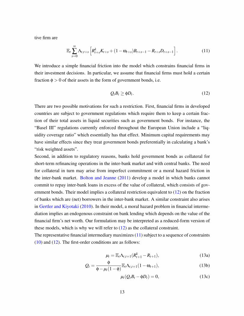
tive firm are

Et

∞

∑s=0

Λt,t+s

[Rk

t+sKt+s +(1−ωt+s)Bt+s−1−Rt+sDt+s−1

]. (11)

We introduce a simple financial friction into the model which constrains financial firms intheir investment decisions. In particular, we assume that financial firms must hold a certainfraction φ > 0 of their assets in the form of government bonds, i.e.

QtBt ≥ φDt . (12)

There are two possible motivations for such a restriction. First, financial firms in developedcountries are subject to government regulations which require them to keep a certain frac-tion of their total assets in liquid securities such as government bonds. For instance, the“Basel III” regulations currently enforced throughout the European Union include a “liq-uidity coverage ratio” which essentially has that effect. Minimum capital requirements mayhave similar effects since they treat government bonds preferentially in calculating a bank’s“risk weighted assets”.Second, in addition to regulatory reasons, banks hold government bonds as collateral forshort-term refinancing operations in the inter-bank market and with central banks. The needfor collateral in turn may arise from imperfect commitment or a moral hazard friction inthe inter-bank market. Bolton and Jeanne (2011) develop a model in which banks cannotcommit to repay inter-bank loans in excess of the value of collateral, which consists of gov-ernment bonds. Their model implies a collateral restriction equivalent to (12) on the fractionof banks which are (net) borrowers in the inter-bank market. A similar constraint also arisesin Gertler and Kiyotaki (2010). In their model, a moral hazard problem in financial interme-diation implies an endogenous constraint on bank lending which depends on the value of thefinancial firm’s net worth. Our formulation may be interpreted as a reduced-form version ofthese models, which is why we will refer to (12) as the collateral constraint.The representative financial intermediary maximizes (11) subject to a sequence of constraints(10) and (12). The first-order conditions are as follows:

µt = EtΛt,t+1(Rkt+1−Rt+1), (13a)

Qt =φ

φ−µt(1−φ)EtΛt,t+1(1−ωt+1), (13b)

µt(QtBt−φDt) = 0, (13c)

13

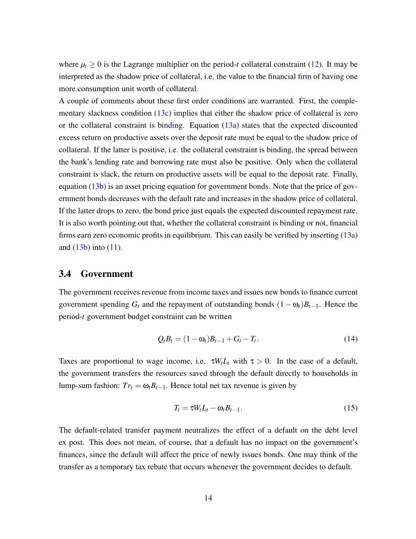
where µt ≥ 0 is the Lagrange multiplier on the period-t collateral constraint (12). It may beinterpreted as the shadow price of collateral, i.e. the value to the financial firm of having onemore consumption unit worth of collateral.A couple of comments about these first order conditions are warranted. First, the comple-mentary slackness condition (13c) implies that either the shadow price of collateral is zeroor the collateral constraint is binding. Equation (13a) states that the expected discountedexcess return on productive assets over the deposit rate must be equal to the shadow price ofcollateral. If the latter is positive, i.e. the collateral constraint is binding, the spread betweenthe bank’s lending rate and borrowing rate must also be positive. Only when the collateralconstraint is slack, the return on productive assets will be equal to the deposit rate. Finally,equation (13b) is an asset pricing equation for government bonds. Note that the price of gov-ernment bonds decreases with the default rate and increases in the shadow price of collateral.If the latter drops to zero, the bond price just equals the expected discounted repayment rate.It is also worth pointing out that, whether the collateral constraint is binding or not, financialfirms earn zero economic profits in equilibrium. This can easily be verified by inserting (13a)and (13b) into (11).

3.4 Government

The government receives revenue from income taxes and issues new bonds to finance currentgovernment spending Gt and the repayment of outstanding bonds (1−ωt)Bt−1. Hence theperiod-t government budget constraint can be written

QtBt = (1−ωt)Bt−1 +Gt−Tt . (14)

Taxes are proportional to wage income, i.e. τWtLt with τ > 0. In the case of a default,the government transfers the resources saved through the default directly to households inlump-sum fashion: Trt = ωtBt−1. Hence total net tax revenue is given by

Tt = τWtLt−ωtBt−1. (15)

The default-related transfer payment neutralizes the effect of a default on the debt levelex post. This does not mean, of course, that a default has no impact on the government’sfinances, since the default will affect the price of newly issues bonds. One may think of thetransfer as a temporary tax rebate that occurs whenever the government decides to default.

14

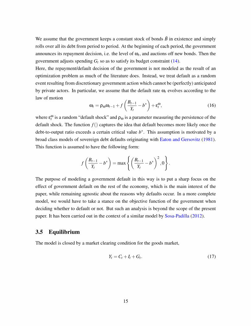
We assume that the government keeps a constant stock of bonds B in existence and simplyrolls over all its debt from period to period. At the beginning of each period, the governmentannounces its repayment decision, i.e. the level of ωt , and auctions off new bonds. Then thegovernment adjusts spending Gt so as to satisfy its budget constraint (14).Here, the repayment/default decision of the government is not modeled as the result of anoptimization problem as much of the literature does. Instead, we treat default as a randomevent resulting from discretionary government action which cannot be (perfectly) anticipatedby private actors. In particular, we assume that the default rate ωt evolves according to thelaw of motion

ωt = ρωωt−1 + f(

Bt−1

Yt−b∗

)+ ε

ωt , (16)

where εωt is a random “default shock” and ρω is a parameter measuring the persistence of the

default shock. The function f () captures the idea that default becomes more likely once thedebt-to-output ratio exceeds a certain critical value b∗. This assumption is motivated by abroad class models of sovereign debt defaults originating with Eaton and Gersovitz (1981).This function is assumed to have the following form:

f(

Bt−1

Yt−b∗

)= max

{(Bt−1

Yt−b∗

)2

,0

}.

The purpose of modeling a government default in this way is to put a sharp focus on theeffect of government default on the rest of the economy, which is the main interest of thepaper, while remaining agnostic about the reasons why defaults occur. In a more completemodel, we would have to take a stance on the objective function of the government whendeciding whether to default or not. But such an analysis is beyond the scope of the presentpaper. It has been carried out in the context of a similar model by Sosa-Padilla (2012).

3.5 Equilibrium

The model is closed by a market clearing condition for the goods market,

Yt =Ct + It +Gt . (17)

15

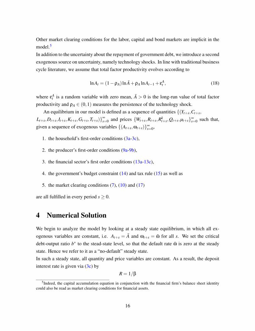
Other market clearing conditions for the labor, capital and bond markets are implicit in themodel.5

In addition to the uncertainty about the repayment of government debt, we introduce a secondexogenous source on uncertainty, namely technology shocks. In line with traditional businesscycle literature, we assume that total factor productivity evolves according to

lnAt = (1−ρA) ln A+ρA lnAt−1 + εAt , (18)

where εAt is a random variable with zero mean, A > 0 is the long-run value of total factor

productivity and ρA ∈ (0,1) measures the persistence of the technology shock.An equilibrium in our model is defined as a sequence of quantities {(Yt+s,Ct+s,

Lt+s,Dt+s, It+s,Kt+s,Gt+s,Tt+s)}∞

s=0 and prices {Wt+s,Rt+s,Rkt+s,Qt+s,µt+s}∞

s=0 such that,given a sequence of exogenous variables {(At+s,ωt+s)}∞

s=0,

1. the household’s first-order conditions (3a-3c),

2. the producer’s first-order conditions (9a-9b),

3. the financial sector’s first order conditions (13a-13c),

4. the government’s budget constraint (14) and tax rule (15) as well as

5. the market clearing conditions (7), (10) and (17)

are all fulfilled in every period s≥ 0.

4 Numerical Solution

We begin to analyze the model by looking at a steady state equilibrium, in which all ex-ogenous variables are constant, i.e. At+s = A and ωt+s = ω for all s. We set the criticaldebt-output ratio b∗ to the stead-state level, so that the default rate ω is zero at the steadystate. Hence we refer to it as a “no-default” steady state.In such a steady state, all quantity and price variables are constant. As a result, the depositinterest rate is given via (3c) by

R = 1/β

5Indeed, the capital accumulation equation in conjunction with the financial firm’s balance sheet identitycould also be read as market clearing conditions for financial assets.

16

and the return on productive assets (the lending rate) is given via (13a) by

Rk = (1+µ)/β.

The government bond price is pinned down by (13b):

Q =βφ

φ−µ(1−φ).

Given the bond price, the collateral constraint (12) determines the amount of deposits andthe capital stock:

D = QB/φ,

K = (1−φ)QB/φ.

Steady state investment is then given by

I = δ(1−φ)QB/φ.

Government spending is found via (14) to be

G = (Q−1)B+ τAFL(K,L)L

Using these results and taking into account (3b), (9b) and (17) one can find steady-stateconsumption and labor by solving the non-linear system:

C = AF(K,L)− I−G.

−UL(C,L) =UC(C,L)AFL(K,L)(1− τ).

Finally, the solution must also satisfy (9a), i.e.

1+µ = β(AFL(K,L)+1−δ).

For our numerical solution, we use an iterative procedure to find the steady state. Guessinginitial values for µ and b∗, we solve for all the endogenous variables and use the last equationto update µ at every step until convergence. We also update b∗ at every iteration. It mustbe noted, that the collateral constraint need not be binding in the steady state. In that case,the model reduces essentially to a standard Real Business Cycle model with a government

17

sector. In our calibration, however, we can exclude this possibility.Because our model is highly nonlinear, an exact analysis of its dynamic behavior is not fea-sible. Therefore, we use a second-order approximation around the steady state just describedto investigate the dynamic effects of exogenous shocks – in particular, a shock to the defaultrate and to the growth rate of total factor productivity.

4.1 Calibration

To perform the numerical simulations, we calibrate the model parameters to match data fromthe Eurozone. In particular, we want the steady state of the model to mimic the pre-crisisperiod between 2000 and 2009. A period in the model is equivalent to one quarter.Household parameters are chosen in line with Kollmann et al. (2016) who estimate a DSGEmodel with a household sector similar to ours using euro area data from 1999 to 2014. Theintertemporal elasticity of substitution σ is 1.4 and the habit persistence in consumption γ

is 0.8. The inverse Frisch elasticity of labor supply is set to 0.45. Furthermore, we set thepure time discount factor β to 0.99 which implies a long-run deposit rate of about 1 percent(about 4 percent on a per-annum basis).For technology parameters, we rely on standard values from the quantitative business cycleliterature. Thus, the capital income share α is set to 0.33, the physical depreciation rate δ is0.025 such that the capital stock lasts for ten years (40 model periods).Turning to the financial sector, the key parameter is the ratio of collateral to total assets φ.As shown in figure (6), the average share of government bonds in total bank assets for is inthe range between 4 and 12 percent. Taking a GDP-weighted of this share yields a value ofabout 9 percent. Hence, in our baseline calibration, we set to φ = 1/11. Since this parameterplays a crucial role in our model, we will also show simulations based on different values ofφ as a robustness check.The stock of government debt B which is rolled over each period is set to 1. The criticaldebt-output ratio b∗ is set to 0.79 and is equal to the steady-state value of B/Y . We setthe tax rate τ to 0.25 which broadly mimics the Eurozone average income tax share. Finally,we choose both ρω and ρA to be 0.75 implying a moderate persistence in the shock processes.

Table (1) shows the steady state values of our calibrated model. All quantity variablesin this table are divided by the steady-state output so that they can be interpreted as GDPshares (the labor supply can be interpreted as the inverse of labor productivity). Differentvalues of φ imply different steady states. Generally, the lower φ, the higher the capital-

18

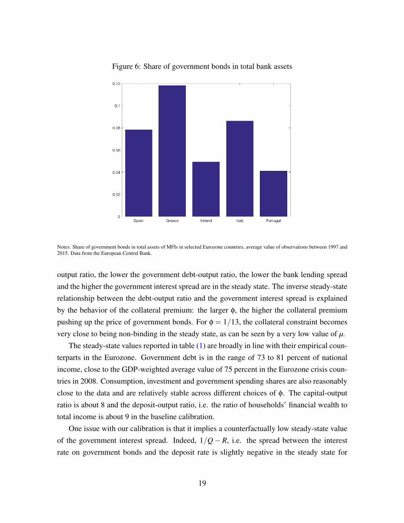
Figure 6: Share of government bonds in total bank assets

Notes: Share of government bonds in total assets of MFIs in selected Eurozone countries, average value of observations between 1997 and2015. Data from the European Central Bank.

output ratio, the lower the government debt-output ratio, the lower the bank lending spreadand the higher the government interest spread are in the steady state. The inverse steady-staterelationship between the debt-output ratio and the government interest spread is explainedby the behavior of the collateral premium: the larger φ, the higher the collateral premiumpushing up the price of government bonds. For φ = 1/13, the collateral constraint becomesvery close to being non-binding in the steady state, as can be seen by a very low value of µ.

The steady-state values reported in table (1) are broadly in line with their empirical coun-terparts in the Eurozone. Government debt is in the range of 73 to 81 percent of nationalincome, close to the GDP-weighted average value of 75 percent in the Eurozone crisis coun-tries in 2008. Consumption, investment and government spending shares are also reasonablyclose to the data and are relatively stable across different choices of φ. The capital-outputratio is about 8 and the deposit-output ratio, i.e. the ratio of households’ financial wealth tototal income is about 9 in the baseline calibration.

One issue with our calibration is that it implies a counterfactually low steady-state valueof the government interest spread. Indeed, 1/Q−R, i.e. the spread between the interestrate on government bonds and the deposit rate is slightly negative in the steady state for

19

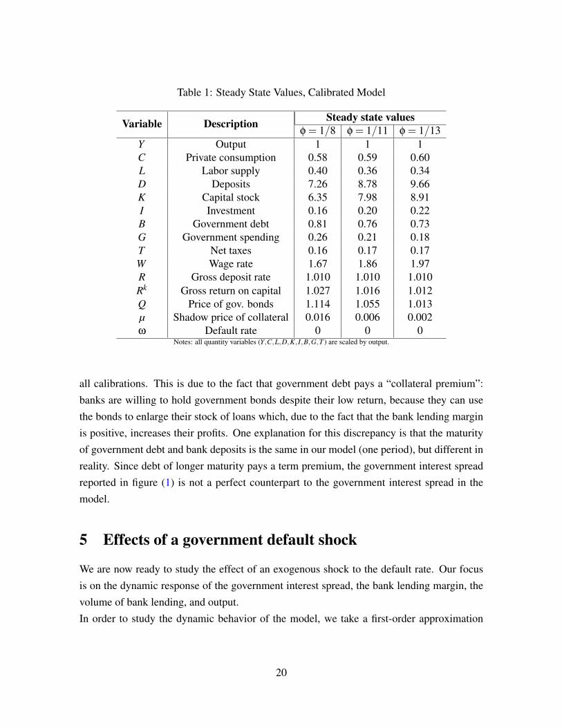
Table 1: Steady State Values, Calibrated Model

Variable Description Steady state valuesφ = 1/8 φ = 1/11 φ = 1/13

Y Output 1 1 1C Private consumption 0.58 0.59 0.60L Labor supply 0.40 0.36 0.34D Deposits 7.26 8.78 9.66K Capital stock 6.35 7.98 8.91I Investment 0.16 0.20 0.22B Government debt 0.81 0.76 0.73G Government spending 0.26 0.21 0.18T Net taxes 0.16 0.17 0.17W Wage rate 1.67 1.86 1.97R Gross deposit rate 1.010 1.010 1.010Rk Gross return on capital 1.027 1.016 1.012Q Price of gov. bonds 1.114 1.055 1.013µ Shadow price of collateral 0.016 0.006 0.002ω Default rate 0 0 0

Notes: all quantity variables (Y,C,L,D,K, I,B,G,T ) are scaled by output.

all calibrations. This is due to the fact that government debt pays a “collateral premium”:banks are willing to hold government bonds despite their low return, because they can usethe bonds to enlarge their stock of loans which, due to the fact that the bank lending marginis positive, increases their profits. One explanation for this discrepancy is that the maturityof government debt and bank deposits is the same in our model (one period), but different inreality. Since debt of longer maturity pays a term premium, the government interest spreadreported in figure (1) is not a perfect counterpart to the government interest spread in themodel.

5 Effects of a government default shock

We are now ready to study the effect of an exogenous shock to the default rate. Our focusis on the dynamic response of the government interest spread, the bank lending margin, thevolume of bank lending, and output.In order to study the dynamic behavior of the model, we take a first-order approximation

20

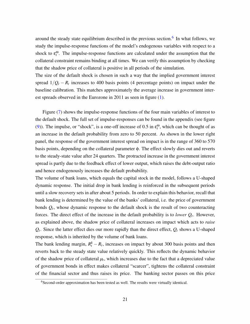
around the steady state equilibrium described in the previous section.6 In what follows, westudy the impulse-response functions of the model’s endogenous variables with respect to ashock to εω

t . The impulse-response functions are calculated under the assumption that thecollateral constraint remains binding at all times. We can verify this assumption by checkingthat the shadow price of collateral is positive in all periods of the simulation.The size of the default shock is chosen in such a way that the implied government interestspread 1/Qt −Rt increases to 400 basis points (4 percentage points) on impact under thebaseline calibration. This matches approximately the average increase in government inter-est spreads observed in the Eurozone in 2011 as seen in figure (1).

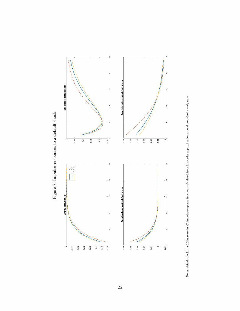
Figure (7) shows the impulse-response functions of the four main variables of interest tothe default shock. The full set of impulse-responses can be found in the appendix (see figure(9)). The impulse, or “shock”, is a one-off increase of 0.5 in εω

t , which can be thought of asan increase in the default probability from zero to 50 percent. As shown in the lower rightpanel, the response of the government interest spread on impact is in the range of 360 to 570basis points, depending on the collateral parameter φ. The effect slowly dies out and revertsto the steady-state value after 24 quarters. The protracted increase in the government interestspread is partly due to the feedback effect of lower output, which raises the debt-output ratioand hence endogenously increases the default probability.The volume of bank loans, which equals the capital stock in the model, follows a U-shapeddynamic response. The initial drop in bank lending is reinforced in the subsequent periodsuntil a slow recovery sets in after about 5 periods. In order to explain this behavior, recall thatbank lending is determined by the value of the banks’ collateral, i.e. the price of governmentbonds Qt , whose dynamic response to the default shock is the result of two counteractingforces. The direct effect of the increase in the default probability is to lower Qt . However,as explained above, the shadow price of collateral increases on impact which acts to raise

Qt . Since the latter effect dies our more rapidly than the direct effect, Qt shows a U-shapedresponse, which is inherited by the volume of bank loans.The bank lending margin, Rk

t −Rt , increases on impact by about 300 basis points and thenreverts back to the steady state value relatively quickly. This reflects the dynamic behaviorof the shadow price of collateral µt , which increases due to the fact that a depreciated valueof government bonds in effect makes collateral “scarcer”, tightens the collateral constraintof the financial sector and thus raises its price. The banking sector passes on this price

6Second-order approximation has been tested as well. The results were virtually identical.

21

Figu

re7:

Impu

lse-

resp

onse

sto

ade

faul

tsho

ck

Not

es:d

efau

ltsh

ock

isa

0.5

incr

ease

inε

ω t,i

mpu

lse-

resp

onse

func

tions

calc

ulat

edfr

omfir

st-o

rder

appr

oxim

atio

nar

ound

no-d

efau

ltst

eady

stat

e.

22

increase by raising the spread between the loan interest rate and the deposit rate. On closerexamination, the increase in the bank lending margin is brought about almost entirely by adrop in the deposit rate Rt while the loan rate Rk

t remains relatively flat. The reason for thisdrop is that banks, confronted with a fall in the value of collateral, reduce their borrowingfrom households so the demand for households’ loanable funds decreases which lowers thedeposit interest rate.Output falls in response to the default shock by about 10 percent relative to its steady-statevalue to which it reverts within the subsequent 16 periods (4 years). This compares wellwith the observed decline in GDP of about 12 percent in the Eurozone crisis countries asseen in figure (4). The decline in output results mainly from the decrease in bank lending(capital stock) and is reinforced by the falling labor supply. Both business investment andgovernment spending falls, while private consumption increases slightly on impact. Theinitial rise in consumption is due to the transfer to households which boosts after-tax incomeand an intertemporal substitution effect resulting from an initial drop in the deposit interestrate. It should be noted, however, that the size of the movement in consumption is less than1 percent of steady-state consumption.In summary, the default shock is able to reproduce the key stylized facts of the Eurozonecrisis, leading to an increase in the government interest spread, a decrease in bank credit, anincrease in the loan-deposit interest differential and a decrease in output and employment.The magnitude of the impulse response functions seem to be broadly similar to the magnitudeof the observed movements in the data. It bears pointing out that the contractionary effectof the default shock has nothing to do with an increase in “uncertainty” or the fear of futuretax increases. It comes entirely and directly from the deterioration of the balance sheet offinancial intermediaries and its subsequent effect on bank credit, capital accumulation andlabor supply.Overall, the results do not appear to be sensitive to the calibrated value of the collateral-to-asset ratio φ. As one might expect, the effects of a default shock are generally stronger(weaker) for higher (lower) values of φ. However, one should bear in mind that decreasingφ below a certain value renders the collateral constraint non-binding in the steady state, inwhich case the dynamic behavior of the model would change substantially. Indeed, if thecollateral constraint is sufficiently lax so that it never binds in steady state as well as forsmall deviations from the steady state, a government default shock is neutral to output, bankcredit and the bank lending margin. Hence, the presence of the financial friction is crucialfor our results.

23

5.1 Effects of an adverse technology shock

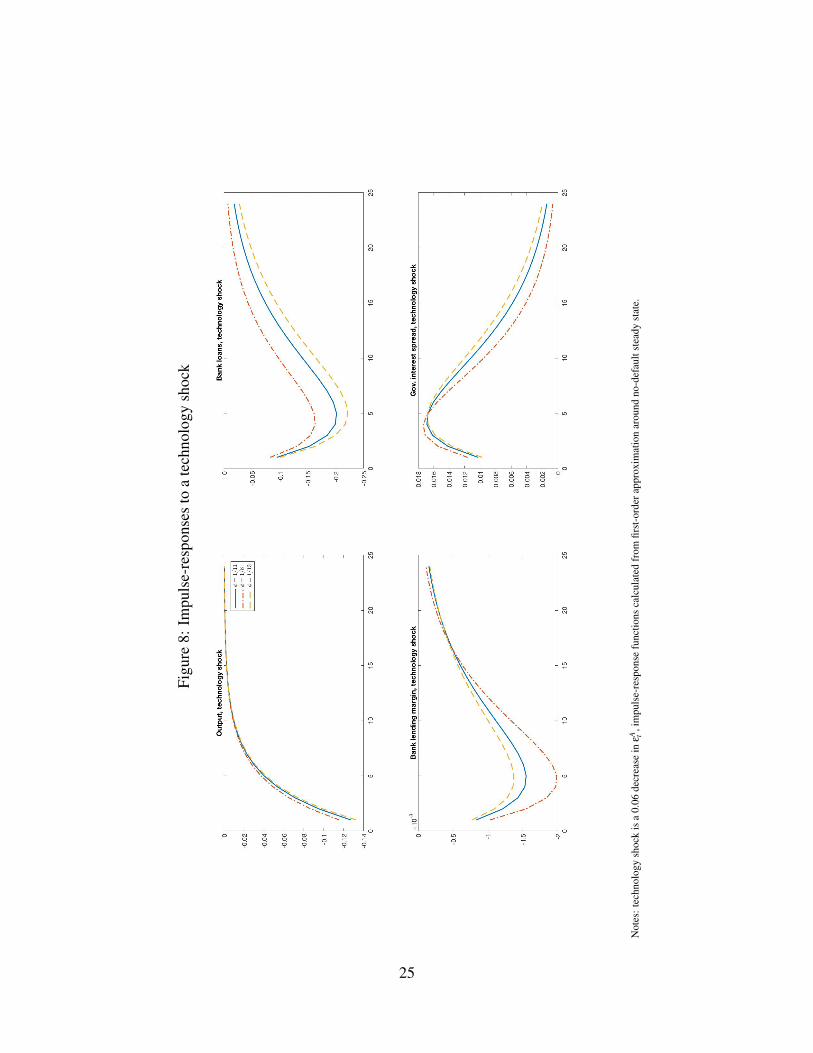
One might ask, however, whether the model allows for a different explanation of the samestylized facts along more “conventional” lines. In particular, the business cycle literature hasfound a significant role for “technology shocks”, i.e. exogenous shifts in the (growth rateof) total factor productivity, in explaining economic fluctuations. Can a technology shockexplain the stylized facts of the Eurozone crisis too?To address this question we simulate the effect of an adverse technology shock. Stock andWatson (2012) have found that a real shock (in particular a shock to the oil price) contributedto the Great Recession in the United States and it is arguable that the Eurozone could havebeen hit in a similar fashion. We calibrate the size of the shock so as to give the same re-sponse to output as the default shock. This turns out to be a shock of −0.06 to εA

t , i.e. a 6percent decrease in total factor productivity.As shown in figure (8), the technology shock depresses output, by design, by about 12 per-cent relative to steady state on impact. Output remains depressed for about 16 periods, justas in the case of the default shock. As a result, the government debt-to-output ratio increaseswhich raises the default rate and thus the government interest spread. But that is not all. Thedecline in total factor productivity also reduces the demand for capital by goods producersand hence the demand for bank loans. This in turn reduces the shadow price of collateralfor financial intermediaries, which reinforces the negative effect on the price of governmentbonds, thus increasing the government interest spread further. Notice that the response tothe technology shock follows the same logic as the response to the default shock, only in re-verse. In both cases, the shadow price of collateral plays the decisive role in the transmissionmechanism.The dynamic behavior of other quantity variables such as the labor supply, investment, gov-ernment spending and net taxes are very similar to the response to the default shock: adecrease on impact followed by a relatively fast return to the steady-state level.7 An ex-ception is the behavior of consumption, which falls on impact due to the negative wealtheffect implied by the technology shock. One can conclude that a technology shock is notdistinguishable from a default shock only by observing their effects on quantities and thegovernment spread.

The shocks can be distinguished, however, by looking at the response of the bank lend-ing margin. Whereas, as we have seen above, the default shock increases the bank lending

7See figures (11) and (12) in the appendix.

24

Figu

re8:

Impu

lse-

resp

onse

sto

ate

chno

logy

shoc

k

Not

es:t

echn

olog

ysh

ock

isa

0.06

decr

ease

inε

A t,i

mpu

lse-

resp

onse

func

tions

calc

ulat

edfr

omfir

st-o

rder

appr

oxim

atio

nar

ound

no-d

efau

ltst

eady

stat

e.

25

margin, the technology shock has the opposite effect. The reason is the differential impactthese shocks have on the shadow price of collateral. As the technology shock lowers de-mand for bank loans, the loan interest rate drops. The interest rate on deposit falls as wellbut by a smaller amount than the loan rate, owing to the fact that collateral has become “lessscarce” relative to total bank assets, which is reflected in a smaller shadow price of collateral.This results indicate that interest rate data, and data on financial assets more broadly, play acrucial role in identifying the source of economic fluctuations. In particular, the technologyshock cannot explain why bank lending margins have increased during the crisis.

6 Discussion and Conclusion

This paper has introduced a financial friction in an otherwise standard business cycle modelby assuming that banks have to hold government bonds as collateral on their balance sheets.We used this model to study the effect of a “government default shock” - an exogenousincrease in the probability of debt default - and concluded that such a shock produces move-ments in the government interest spread, bank credit, bank lending margin and output thatroughly match the observed behavior of these variables in the Eurozone crisis. We have alsoshown that a negative technology shock - an exogenous decrease in total factor productivity- can explain some but not all of these observations.The shadow price of collateral - the marginal value to financial firms of having an additionalunit of collateral - plays a key role in the transmission of shocks. The negative consequencesof a government default are driven only by the effect on banks’ balance sheets and the as-sociated increase in the effective scarcity of the collateral assets which is reflected in itsshadow price, not by any increase in economic “uncertainty” or the fear of future tax in-creases. While the shadow price of collateral cannot be directly observed, the papers showsthat it is reflected in the spread between the interest rates on loans and deposit, the banklending margin. This underscores the importance of financial price variables in identifyingthe sources of structural economic shocks.We have kept the model in this paper deliberately simple in that we left out many of the fric-tions that have been found important in explaining business cycles. For instance, we haveabstracted entirely from nominal rigidities and foreign trade. Incorporating these featuresin the model would no doubt improve its usefulness for empirical work as well as provideadditional insights in the transmission of government default to other macroeconomic vari-

26

ables. One of the open questions in that respect is to what extend monetary policy can helpto shield the economy from the detrimental effects of government default in the presence offinancial frictions. Another is how government default can spill over into foreign countries.These could be worthwhile endeavors for future research.

References

Acharya, V., Drechsler, I., and Schnabl, P. (2014). A pyrrhic victory? bank bailouts andsovereign credit risk. Journal of Finance, 69(6):2689–2739.

Bocola, L. (2016). The pass-through of sovereign risk. Journal of Political Economy,124(4):879–926.

Bolton, P. and Jeanne, O. (2011). Sovereign default risk and bank fragility in financiallyintegrated economies. IMF Economic Review, 59(2):162–194.

De Bruyckere, V., Gerhardt, M., Schepens, G., and Vander Vennet, R. (2013).Bank/sovereign risk spillovers in the european debt crisis. Journal of Banking and Fi-

nance, 37(12):4793–4809.

Eaton, J. and Gersovitz, M. (1981). Debt with potential repudiation: Theoretical and empir-ical analysis. The Review of Economic Studies, 48(2):289–309.

Fernandez-Villaverde, J., Ramírez, J. F. R., and Schorfheide, F. (2016). Solution and esti-mation methods for dsge models. Working Paper 21862, National Bureau of EconomicResearch.

Gennaioli, N., Martin, A., and Rossi, S. (2014). Sovereign default, domestic banks, andfinancial institutions. The Journal of Finance, 69(2):819–866.

Gertler, M. and Kiyotaki, N. (2010). Financial Intermediation and Credit Policy in BusinessCycle Analysis. In Friedman, B. M. and Woodford, M., editors, Handbook of Monetary

Economics, volume 3 of Handbook of Monetary Economics, chapter 11, pages 547–599.Elsevier.

Kollmann, R., Pataracchia, B., Raciborski, R., Ratto, M., Roeger, W., and Vogel, L. (2016).The post-crisis slump in the Euro Area and the US: Evidence from an estimated three-region DSGE model. European Economic Review, 88(C):21–41.

27

Mody, A. and Sandri, D. (2012). The eurozone crisis: how banks and sovereigns came to bejoined at the hip. Economic Policy, 27(70):199–230.

Shambaugh, J. (2012). The euro’s three crises. Brookings Papers on Economic Activity, 44(1(Spring)):157–231.

Sosa-Padilla, C. (2012). Sovereign Defaults and Banking Crises. Department of EconomicsWorking Papers 2012-09, McMaster University.

Stock, J. H. and Watson, M. W. (2012). Disentangling the channels of the 2007–09 recession.Brookings Papers on Economic Activity, 2012(1):81–135.

7 Appendix

The full non-linear model is described by equations (3a-3c), (7), (9a-9b), (10), (13a-13c),(14), (15), (17) as well as (16) and (18). It can be written in the form

EtF(xt+1,xt ,xt−1,ut) = 0,

where xt is the vector of endogenous variables, and ut is the vector of shocks εωt and εA

t .The function F() is implicitly defined by the model equations. Solving the model involvesfinding a policy function g() such that

xt = g(xt−1,ut),

relating current endogenous variables to past realizations and current shocks. Plugging inthe policy functions repeatedly in the above equation yields

EtF(g(g(xt−1,ut),ut+1),g(xt−1,ut),xt−1,ut) = 0,

We take a first-order Taylor series expansion around the steady-state point F(x,x,x,0):

Et [Fx,+(gxgxxt−1 +guut +guut+1)+Fx,0(gxx+guut)+Fx,−xt−1 +Fuut ] = 0,

where xt−1 = xt−1− x, Fx,+ = ∂F/∂xt+1, Fx,0 = ∂F/∂xt , Fx,− = ∂F/∂xt−1 , gx = ∂F/∂xt−1

and gu = ∂g/∂ut . The derivatives gx and gu can be recovered using the techniques described

28

in Fernandez-Villaverde et al. (2016) yielding a linear approximation of the form

xt = gxxt−1 +guut ,

from which it is straightforward to calculate impulse-response functions. It should be notedthat the linear approximation is only good for small perturbations from the initial point. Allcalculations in these paper are carried out using the Dynare tool on MATLAB. The code isavailable from the author upon request.

29

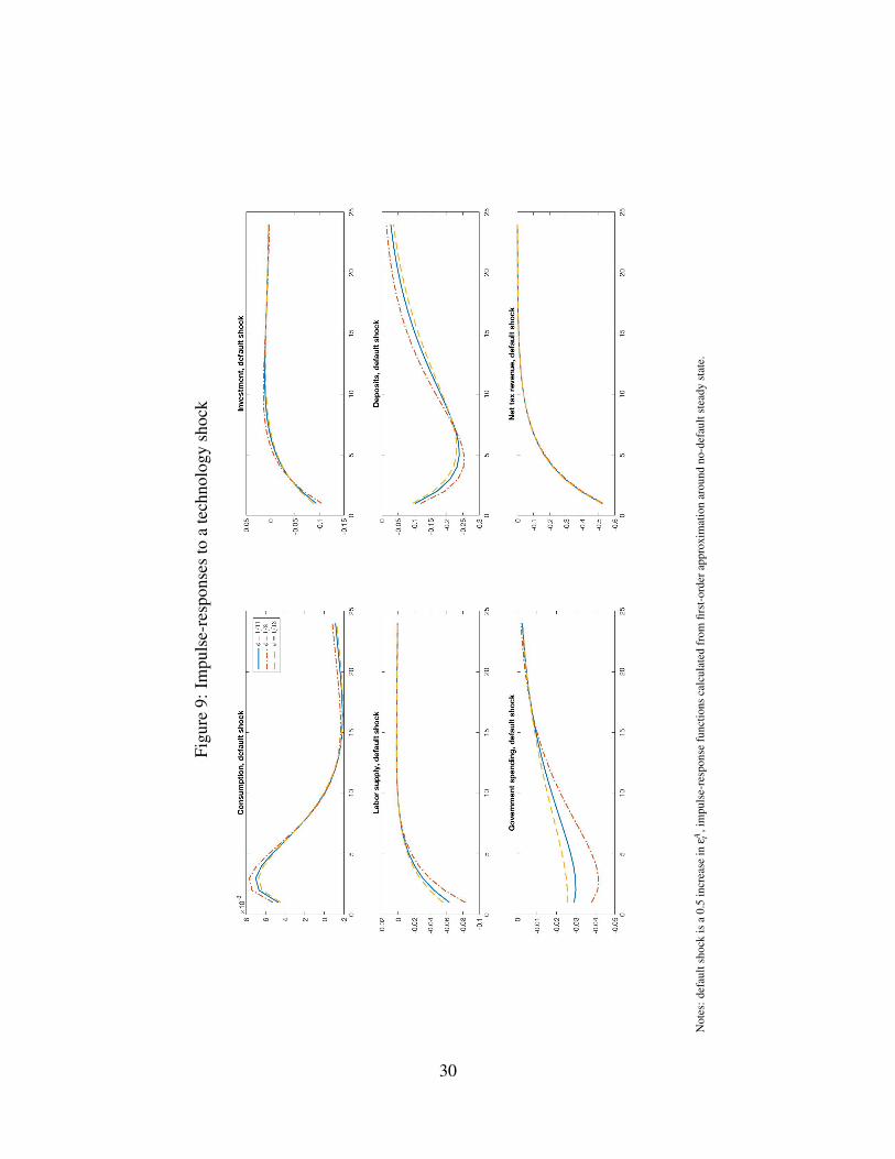
Figu

re9:

Impu

lse-

resp

onse

sto

ate

chno

logy

shoc

k

Not

es:d

efau

ltsh

ock

isa

0.5

incr

ease

inε

A t,i

mpu

lse-

resp

onse

func

tions

calc

ulat

edfr

omfir

st-o

rder

appr

oxim

atio

nar

ound

no-d

efau

ltst

eady

stat

e.

30

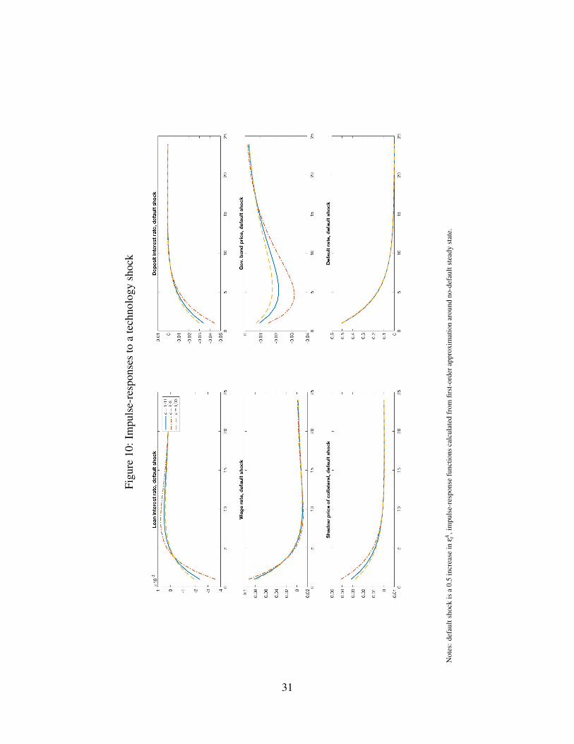
Figu

re10

:Im

puls

e-re

spon

ses

toa

tech

nolo

gysh

ock

Not

es:d

efau

ltsh

ock

isa

0.5

incr

ease

inε

A t,i

mpu

lse-

resp

onse

func

tions

calc

ulat

edfr

omfir

st-o

rder

appr

oxim

atio

nar

ound

no-d

efau

ltst

eady

stat

e.

31

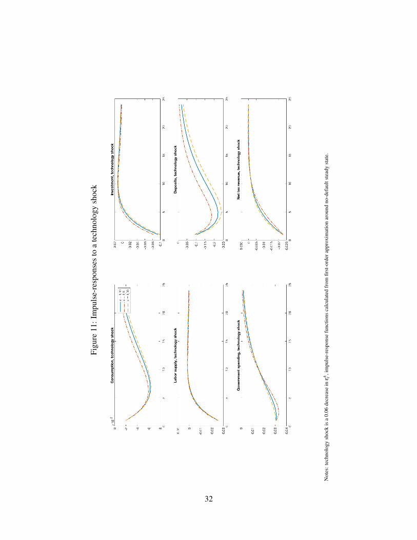
Figu

re11

:Im

puls

e-re

spon

ses

toa

tech

nolo

gysh

ock

Not

es:t

echn

olog

ysh

ock

isa

0.06

decr

ease

inε

A t,i

mpu

lse-

resp

onse

func

tions

calc

ulat

edfr

omfir

st-o

rder

appr

oxim

atio

nar

ound

no-d

efau

ltst

eady

stat

e.

32

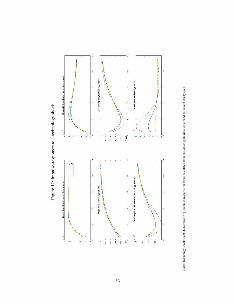
Figu

re12

:Im

puls

e-re

spon

ses

toa

tech

nolo

gysh

ock

Not

es:t

echn

olog

ysh

ock

isa

0.06

decr

ease

inε

A t,i

mpu

lse-

resp

onse

func

tions

calc

ulat

edfr

omfir

st-o

rder

appr

oxim

atio

nar

ound

no-d

efau

ltst

eady

stat

e.

33