the social desirability of belief in god · the social desirability of belief in god simon jackman...
TRANSCRIPT

THE SOCIAL DESIRABILITY OF BELIEF IN GOD
SIMON JACKMAN
STANFORD UNIVERSITY

simon jackman - BAMM - march 2007
Religion in American politics
overwhelming majorities of survey respondents report belief in God (80% - 90%).
U.S. exceptional in this regard.
role of religion in recent American political debate

simon jackman - BAMM - march 2007
Don't believe
-75% -50% -25% 0% 25% 50% 75% 100%
ChilePhilippines
CyprusUSA
PortugalIreland
N IrelandItaly
SpainSlovakia
AustriaNew
HungaryAustralia
SwitzerlandGreat
Germany-WLatvia
NetherlandsNorway
SloveniaBulgaria
RussiaFrance
DenmarkCzech Rep
JapanSweden
Germany-E
Belief (%)
Don't know
Higher power
Believe sometimes
Believe w/ doubt
Believe, no doubt
Courtesy of Mike Hout.
Cross-national rates of belief in God &/or “higher power”, International Social Survey Program.
simon jackman - BAMM - march 2007
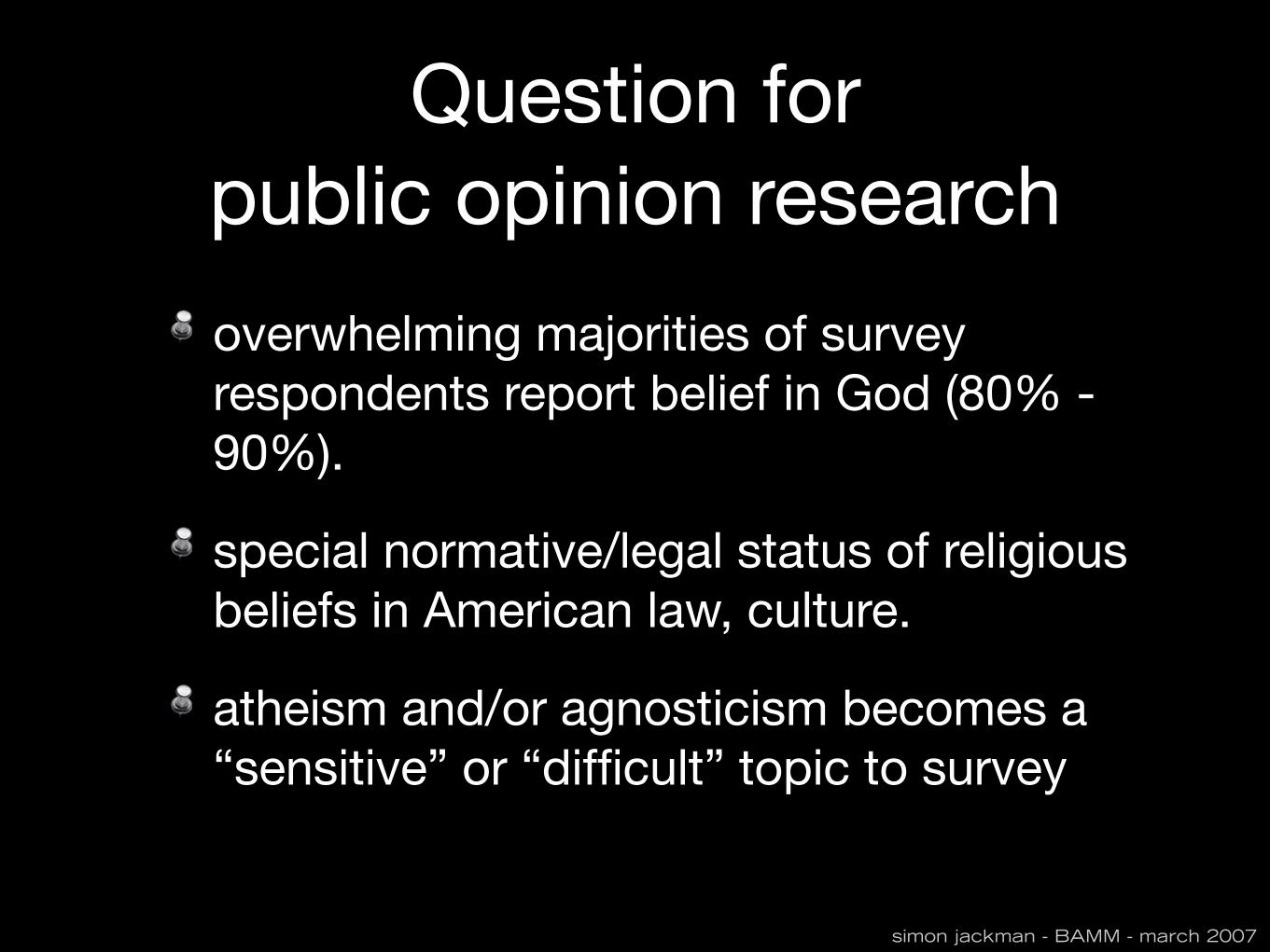
Question for public opinion research
overwhelming majorities of survey respondents report belief in God (80% - 90%).
special normative/legal status of religious beliefs in American law, culture.
atheism and/or agnosticism becomes a “sensitive” or “difficult” topic to survey

simon jackman - BAMM - march 2007
Empirical Project
can we get rid of any “social-desirability” bias in conventional measures of proportions of believers/atheists?
• drug use
• sexual behavior
• voter turnout
all instances of “sensitive topics”

simon jackman - BAMM - march 2007
Implementation in 2006 CCES
on-line is “self-completion”; hence plausible that less social-desirability effects than face-to-face
randomized response methods difficult to implement on-line (credibility of randomization)

simon jackman - BAMM - march 2007

yij ! Bernoulli(hj)
E(yij) = hj
E(yi) =!
j
hj
y = n-1
n!
i=1
yi
E(y) = n-1
n!
i=1
E(yi) = n-1
n!
i=1
!
j
hj
=!
hj
simon jackman - BAMM - march 2007
List Experiments

• In control condition, E(yC) =!J
j=1 hj
• In treatment condition, E(yT ) =!J+1
j=1 hj
• Hence E(yT - yC) =!J+1
j=1 hj -!J
j=1 hj = hJ+1
• Inference (standard errors, confidence intervals) isstraightforward.
simon jackman - BAMM - march 2007
List Experiments

simon jackman - BAMM - march 2007
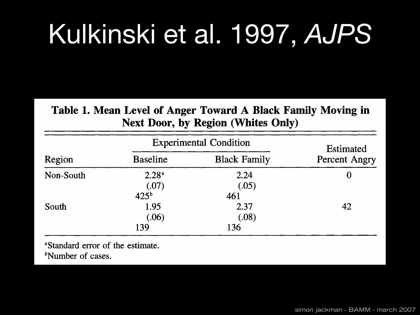
Kulkinski et al. 1997, AJPS
simon jackman - BAMM - march 2007
Kulkinski et al. 1997, AJPS

simon jackman - BAMM - march 2007
Data
2006 CCES, through Polimetrix
2 batches of 1,000 respondents (“Stanford” and “PMX”)
Randomization to treatment and control takes place as respondents administered survey
Post-stratification weights applied

simon jackman - BAMM - march 2007
Split-third design
Please look over the statements below. Please just tell us how many apply to you. We don't want to know which statements apply to you, just how many.
• I have had dreams in which I see myself dying.
• I believe in life after death.
• I believe miracles sometimes happen.
Treatment 1: adds “I do not believe in God”
Treatment 2: adds “I believe in God”

simon jackman - BAMM - march 2007
Randomization
After matched/selected subject voluntarily opt-ins to web survey, then randomization takes place.
Post-stratification weights provided. Range from .5 to 3.5.
Do we have balance across branches of experiment?

• Educational attainment, three ordinal categories.!
24 = 7.24, p = .12. ANOVA: F2,456 = 1.41, p = .244
• Ideological self-placement, three categories. !24 = 3.44,
p = .49. ANOVA: F2,965 = .03, p = .97.
• Self-reported frequency of church attendance, fourordinal categories. !
26 = 16.3, p = .012. ANOVA:
F2,972 = .21, p = .812.
simon jackman - BAMM - march 2007
Balance checkin Stanford batch

simon jackman - BAMM - march 2007
# Items Agreed With0 1 2 3 4 Mean n Std.Err
Treatment 2:Adding Believe in God 9 8 15 52 16 2.59 345 0.061
Treatment 1:Adding Not Believe in God 5 16 55 19 5 2.02 318 0.048
Control Group 12 20 52 16 1.72 325 0.048
Table 1: Cell entries are row percentages (may not sum to 100 due to rounding). StanfordUniversity component of CCES 2006 (weighted data).
# Items Agreed With0 1 2 3 4 Mean n Std.Err
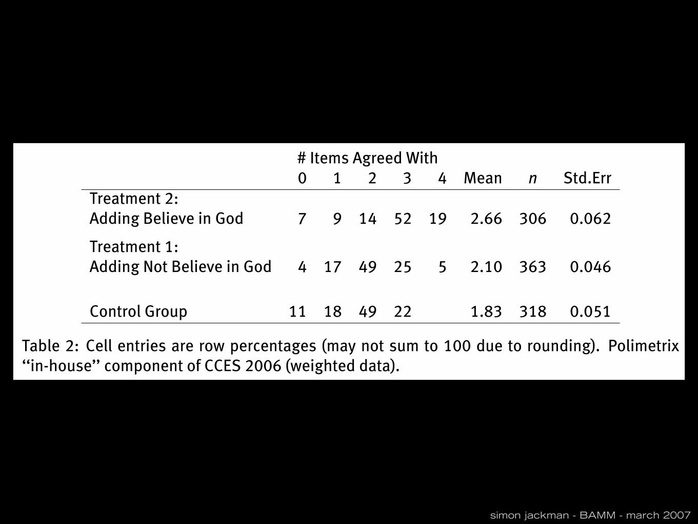
Treatment 2:Adding Believe in God 7 9 14 52 19 2.66 306 0.062
Treatment 1:Adding Not Believe in God 4 17 49 25 5 2.10 363 0.046
Control Group 11 18 49 22 1.83 318 0.051
Table 2: Cell entries are row percentages (may not sum to 100 due to rounding). Polimetrix‘‘in-house’’ component of CCES 2006 (weighted data).
Stanford PMXAtheists .30 .27
[.17, .43] [.14, .41]
Theists .87 .83[.71, 1.02] [.67, .99]
Total 1.17 1.10[.97, 1.38] [.89, 1.31]
Pr(Total>1) .96 .83
Table 3: Estimates of Population Incidences of Atheism and ‘‘Belief in God’’, Identical ListExperiments in Stanford and PMX components of CCES 2006. Asymptotic ninety-five percentconfidence intervals in brackets.
3
simon jackman - BAMM - march 2007
# Items Agreed With0 1 2 3 4 Mean n Std.Err
Treatment 2:Adding Believe in God 9 8 15 52 16 2.59 345 0.061
Treatment 1:Adding Not Believe in God 5 16 55 19 5 2.02 318 0.048
Control Group 12 20 52 16 1.72 325 0.048
Table 1: Cell entries are row percentages (may not sum to 100 due to rounding). StanfordUniversity component of CCES 2006 (weighted data).
# Items Agreed With0 1 2 3 4 Mean n Std.Err
Treatment 2:Adding Believe in God 7 9 14 52 19 2.66 306 0.062
Treatment 1:Adding Not Believe in God 4 17 49 25 5 2.10 363 0.046
Control Group 11 18 49 22 1.83 318 0.051
Table 2: Cell entries are row percentages (may not sum to 100 due to rounding). Polimetrix‘‘in-house’’ component of CCES 2006 (weighted data).
Stanford PMXAtheists .30 .27
[.17, .43] [.14, .41]
Theists .87 .83[.71, 1.02] [.67, .99]
Total 1.17 1.10[.97, 1.38] [.89, 1.31]
Pr(Total>1) .96 .83
Table 3: Estimates of Population Incidences of Atheism and ‘‘Belief in God’’, Identical ListExperiments in Stanford and PMX components of CCES 2006. Asymptotic ninety-five percentconfidence intervals in brackets.
3

simon jackman - BAMM - march 2007
Stanford PMXAtheists .30 .27
[.17, .43] [.14, .41]
Theists .87 .83[.71, 1.02] [.67, .99]
Total 1.17 1.10[.97, 1.38] [.89, 1.31]
Pr(Total>1) .96 .83
Estimates of Population Proportions

simon jackman - BAMM - march 2007
Stratification
Atheist Rate
Stanford PMX
Low Education .17(.11)
.27(.11)
Medium Education
.33(.09)
.20(.09)
High Education.61(.23)
.80(.25)
simon jackman - BAMM - march 2007
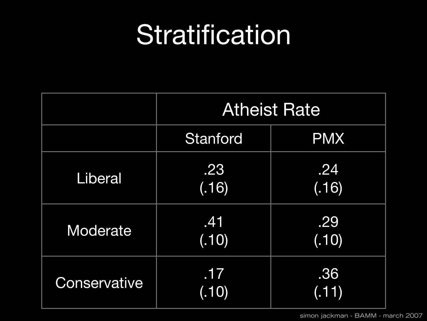
Stratification
Atheist Rate
Stanford PMX
Liberal .23(.16)
.24(.16)
Moderate .41(.10)
.29(.10)
Conservative.17(.10)
.36(.11)
simon jackman - BAMM - march 2007
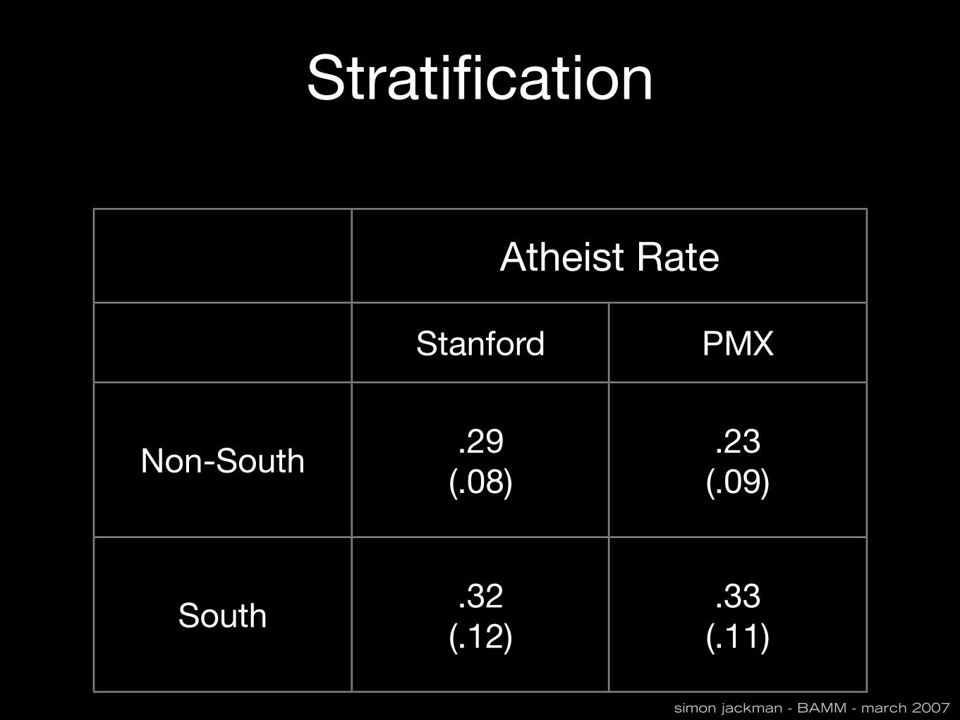
Stratification
Atheist Rate
Stanford PMX
Non-South .29(.08)
.23(.09)
South .32(.12)
.33(.11)

simon jackman - BAMM - march 2007
Stratification
Atheist Rate
Stanford PMX
< $40K.002(.12)
.11(.14)
$40K-$100K.35(.11)
.39(.10)
> $100K.46(.18)
.39(.17)

simon jackman - BAMM - march 2007
Stratification
Atheist Rate
Self-reported church attendance Stanford PMX
Once a week or more
.15(.10)
.05(.11)
A few times a month
.21(.22)
.41(.20)
Less than once a month
.08(.15)
.18(.15)
Almost never or never
.49(.11)
.37(.11)

simon jackman - BAMM - march 2007
Future
Better baseline calibration: ask “innocuous” items one-by-one in the control group.
Can then relate to covariates, generate predicted probabilities by covariate class in treated groups.
Can then estimate predicted probability of assent to “sensitive” proposition for each treated subject. See Corstange (2006).
simon jackman - BAMM - march 2007
Conclusion
Twice as many atheists as you might think...?
Need further work to replicate/validate/elaborate the finding.