the skills to pay the bills: returns to on-the-job soft

The Skills to Pay the Bills:

Returns to On-the-job Soft Skills Training*

Achyuta Adhvaryu

University of Michigan & NBER

Namrata Kala

Harvard University

Anant Nyshadham

Boston College

November 2016

Abstract

The willingness of firms to provide general training to workers depends on the productivity gainsfrom training and the likelihood that workers are retained. We evaluate the impacts of training insoft skills development on the workplace outcomes of female garment workers in Bengaluru, India.We implemented a lottery determining access to the program by randomizing lines and then work-ers within lines to treatment, which allows us to capture treatment effects and program spillovers.We find that despite a high overall turnover rate, more treated workers are retained during thetraining period; this difference disappears after training is complete. Treated workers are 12 percentmore productive than controls. Within-team spillovers in productivity and task complexity are sub-stantial. Survey outcomes support the hypothesis that the program increased the stock of soft skills,which raised workers’ marginal products. Wages increase by 0.5 percent after program completion.Pairing our point estimates with program costs, we calculate that the net return to on-the-job softskills training for garment workers is large – about 250 percent 9 months after program completion.

Keywords: general training, soft skills, productivity, ready-made garmentsJEL Codes: J24, M53, O15

*We are incredibly grateful to Anant Ahuja, Chitra Ramdas, Raghuram Nayaka, Sudhakar Bheemarao, Paul Ouseph,and for their coordination, enthusiasm, and guidance. Thanks to Dotti Hatcher, Lucien Chan, Noel Simpkin, and others atGap, Inc. for their support and feedback on this work. We acknowledge funding from Private Enterprise Development inLow-Income Countries (PEDL) initiative, and Adhvaryu’s NIH/NICHD (5K01HD071949) career development award. Thisresearch has benefited from discussions with Rocco Macchiavello, Dilip Mookherjee, Claudia Olivetti, Antoinette Schoar,Chris Woodruff, and Chris Udry, and seminar audiences at PEDL, the IGC (London and Dhaka), the World Bank, Michigan,and Georgetown. Many thanks to Robert Fletcher and Aakash Mohpal for excellent research assistance. The views expressedherein do not represent PEDL, NIH, Gap, Inc., or Shahi Exports. All errors are our own.

1

1 Introduction

Does it pay for firms to provide general training to workers? Firms’ returns depend on the productivity

gains from training and the likelihood that workers are retained. In high-turnover environments, and

especially if training itself increases turnover (as workers receive better wage offers at other firms),

even programs that generate large productivity returns may not be appealing investments for firms

(Becker, 1964). On the other hand, labor market imperfections, such as search frictions and informa-

tion asymmetries, can generate value to general training even in thick labor markets (Acemoglu, 1997;

Acemoglu and Pischke, 1998, 1999; Autor, 2001; Chang and Wang, 1996; Katz and Ziderman, 1990), a

result that squares with the fact that most firms provide general training to workers without accompa-

nying wage reductions (e.g., Bassanini et al. (2007)).

Quantifying the impacts of general training – on productivity as well as retention – is thus of

paramount importance. In this paper, we evaluate the workplace impacts of a general training pro-

gram focusing on soft skills development. There is emerging consensus on the importance of soft

skills – for example, the effective allocation of time and money, teamwork, leadership, relationship

management, and acquiring and assimilating information – for labor market success (Deming, 2015;

Groh et al., 2015; Guerra et al., 2014; Heckman and Kautz, 2012; Heckman et al., 2006). Global surveys

of employers corroborate that these skills are in high demand (Cunningham and Villasenor, 2016).

We know from recent work that it is possible to inculcate soft skills in early childhood and, to an

extent, in early adolescence (Attanasio et al., 2014; Gertler et al., 2014; Grantham-McGregor et al., 1991;

Ibarraran et al., 2015). But how malleable these skills are in adulthood is an open question. Structural

estimates of dynamic human capital accumulation models suggest that it may be very difficult to af-

fect the stock of skills at later ages, particularly for those with low baseline stocks, due to dynamic

complementarities (Aizer and Cunha, 2012; Cunha et al., 2010; Heckman and Mosso, 2014).

Yet the need for trained workers – in terms of both hard (technical) and soft skills – has never been

greater, especially in low-income countries, where industrial growth has far outstripped growth in the

supply of skilled labor (Cunningham and Villasenor, 2016; Hanushek, 2013). On-the-job training has

always played a crucial role in building workforce human capital (Becker, 1964). In countries with low

public sector capacity, it is all the more true that skilling takes place within the firm (Tan et al., 2016).

The questions that motivate the present study, then, are threefold. First, is it possible to improve

soft skills meaningfully for adults with low stocks of these skills? Second, if skills do improve, what

2

are the workplace consequences, including impacts on productivity and retention? Finally does it pay

for firms to impart this form of general training to their workers?

To answer these questions, we partnered with the largest ready-made garment export firm in In-

dia to evaluate an intensive, workplace-based soft skills training program. The initiative, the Personal

Advancement and Career Enhancement (P.A.C.E.) program, aims to empower female garment work-

ers (FGWs) via training in a broad variety of life skills, including modules on communication, time

management, financial literacy, successful task execution, and problem-solving. We conducted a ran-

domized controlled trial (RCT) in five garment factories in Bengaluru, a large city in southern India.

We assessed the impacts of soft skills training on 1) measures of the stock of these skills via survey;

and 2) workplace outcomes such as retention, productivity, and salary. The trial’s design allows us

to capture spillovers onto untreated workers, both through the transfer of skills as well as through

production complementarities. Finally, we compute the firm’s returns, combining our point estimates

with data on the program’s costs and the firm’s accounting profits.

We used a two-stage randomization procedure. We enrolled female garment workers (FGWs) in a

lottery for the chance to take part in the P.A.C.E. program. In the first stage, we randomized production

lines to treatment. In the second stage, within treatment lines, we randomized workers who had en-

rolled in the lottery to either direct P.A.C.E. training or spillover treatment. We thus estimate treatment

effects by comparing trained workers (on treatment lines) to control workers on control lines (who

enrolled in the lottery but whose lines were assigned to control). We estimate spillovers by comparing

untrained workers on treatment lines to control workers on control lines.

Direct impacts on workplace outcomes, measured using the firm’s administrative data, are con-

sistent with the acquisition of soft skills by workers. Treated workers are more productive and more

likely to be assigned to complex tasks. Impacts last up to 9 months after program completion (when

we ceased data collection), suggesting that learned skills translated into persistent improvements in

workplace outcomes. The program did not cause workers to leave the firm: retention actually im-

proved in the treatment group relative to the control during the program period; this treatment effect

diminished after program completion.

Results from a survey administered to treatment and control workers in the month after pro-

gram completion complement these impacts on workplace outcomes. First, treatment workers exhibit

greater acquisition and use of information: they are more likely to avail themselves of skill develop-

ment initiatives at the firm, state-sponsored pension and subsidized health-care. Second, consistent

3

with improved resource management, particularly financial literacy and forward-looking behavior,

treatment workers were more likely to be saving for their own or their children’s education, have

more rational risk and time preferences, and have higher aspirations for children’s ultimate educa-

tional attainment. Third, survey results indicate greater self-assessment of workplace quality (relative

to production line peers), consistent with an increase in self-regard. Finally, pre/post data from assess-

ment tools designed to measure learning in each of the program’s modules show that treated workers

significantly improved their stocks of knowledge in each one of the program’s target areas. Taken in

sum, the results indicate that the program effectively increased workers’ stocks of soft skills.

The weight of the evidence we present suggests that the primary mechanism for improvements

in workplace outcomes was the inculcation of soft skills. Our interpretation of the results is that skills

like time and stress management; communication; problem solving and decision-making; and effective

teamwork are “soft” inputs into production. Reinforcing these skills thus directly affects productivity.

Retention went up relative to control during the program period likely because workers were receiv-

ing an in-kind transfer, thus increasing the likelihood that their effective wage at the firm lay above the

wage at their best outside option. Team spillovers were likely generated both by the transfer of skills

from treated to untreated team members, as well as by way of technical production complementari-

ties.1

The two-stage randomization design allows us to examine treatment spillovers within teams (pro-

duction lines). We find that untrained workers on treatment lines have more cumulative person days

compared to control workers (on control lines) during the program. They are also more productive

and are assigned to more complex operations. These impacts are nearly as large as the direct impacts

of treatment, suggesting that treated workers boosted overall team performance.

Finally, we combine our point estimates of impacts on workplace outcomes with program cost and

accounting profit data to calculate the costs and benefits of the program to the firm. The program’s net

rate of return was already considerable by the end of the program period (12%), with the program costs

more than covered. By the end of the measurement period, nine months after program completion,

the return was about 250%. These very large returns are rationalized by the relatively low costs of the

1A reciprocity motive is another potential mechanism for changes in workplace outcomes, but our results suggest theimpacts we find are not substantively driven by this factor. In addition to the direct survey evidence on changes in soft skills,two facts indicate that the role for reciprocity in our context is likely small. First, we observe spillover impacts on workerswho enrolled in the lottery for the program but were not chosen for P.A.C.E. treatment (and work on the same lines as treatedworkers). Second, we observe persistent impacts on productivity that last up to 9 months after program completion. Thelimited role of reciprocity is consistent with recent work on gift-giving in the workplace (DellaVigna et al., 2016).

4

program combined with the accumulated effects on productivity and person days, and are consistent

with other recent interventions in garment factories (Menzel, 2015).

Our study informs the understanding of firms’ returns to providing general training for workers.

Previous work has sought to quantify the productivity impacts of on-the-job training using observa-

tional data on firms and workers in the United States and Western Europe (Barrett and O’Connell,

2001; Barron et al., 1999; Dearden et al., 2006; Konings and Vanormelingen, 2015; Mincer, 1962). These

studies tend to find that training increases productivity, but there is disagreement on the magnitude

of this increase (Blundell et al., 1999). Specifically, when endogeneity of training is credibly accounted

for (e.g., using matching methods), productivity returns become very small (Goux and Maurin, 2000;

Leuven and Oosterbeek, 2008).

We add to this literature in several ways. First, we estimate causal effects by exploiting randomized

assignment to training, which overcomes potential self-selection bias (Altonji and Spletzer, 1991; Bartel

and Sicherman, 1998). Second, we estimate impacts on retention in addition to productivity; retention

is crucial to understanding firms’ overall returns to training but has not been examined thus far. Third,

we carry out our experiment in a low-income country setting – where training frontline workers might

have large potential given low levels of baseline skills – while existing studies use data from firms in

high-income countries.

Our experiment also serves as a proving ground for influential theories of firms’ decisions to pro-

vide general training (Acemoglu, 1997; Acemoglu and Pischke, 1998, 1999; Autor, 2001; Becker, 1964).

Broadly consistent with the predictions of Acemoglu (1997); Acemoglu and Pischke (1998, 1999); Au-

tor (2001) (and against Becker’s original hypothesis), we find that 1) general training does not increase

worker attrition, despite high overall turnover (indeed, during the program, workers are more likely to

remain with the firm); and 2) the increase in wages for treated workers is not commensurate with the

productivity response (wage increases by 0.5 percent, while productivity increases by 11-12 percent).

This set of results suggests that labor market frictions – search costs or information asymmetry or both

– are likely substantial in our setting.

We also contribute to the literature examining the labor market impacts of soft skills (Deming,

2015; Groh et al., 2015; Guerra et al., 2014; Heckman and Kautz, 2012; Heckman et al., 2006; Riordan

and Rosas, 2003). Growing interest in active labor market policies (Heckman et al., 1999) in low-income

countries has spurred high-quality research on the impacts of vocational training programs, which of-

ten include a soft skills training component (Betcherman et al., 2004). In general, evidence on the labor

5

market benefits of training is mixed. An intervention focused on young women finds positive impacts

on some outcomes (Buvinic and Furst-Nichols, 2016). The only other study to our knowledge that

evaluates (via randomized assignment) the impacts of soft skills separately from other types of train-

ing, Groh et al. (2012), examines the impacts of soft skills training (and separately, wage subsidies) for

female community college graduates in Jordan. Treatment effects on the probability of employment,

work hours, and income appear to be quite small. Our study takes a complementary approach by

targeting a popuplation of young workers who are already employed and for whom high frequency

observation of workplace outcomes is possible.

Finally, we contribute to the literature on female labor force participation and workplace outcomes.

Female participation in the labor force has stagnated globally and has recently been falling (Morton

et al., 2014). In India, it is not only unusually low (India ranks 120th out of 131 countries (Chatterjee

et al., 2015)), but has experienced a substantial reduction in the share of women working in rural ar-

eas between 1987 and 2009, despite a fertility transition and relatively robust economic growth (Afridi

et al., 2016). Studying improvements in career prospects for women, via managerial training and pro-

motion as Macchiavello et al. (2015) do, or via soft-skills training and resulting productivity enhance-

ments as we do, can contribute to understanding determinants of female labor force participation that

are amenable to policy intervention.

The rest of the paper is organized as follows. Section 2 discusses the garment production context

and reviews the details of the training program and the experimental design. Section 3 discusses the

data sources and the construction of key variables, and section 4 describes the estimation strategy. Sec-

tion 5 describes the results of the estimation. Section 6 discusses and evaluates possible mechanisms,

and section 7 concludes with an analysis of the costs and benefits to the firm.

2 Context, Program Details, and Experiment Design

2.1 Context

2.1.1 Ready-made Garments in India

Apparel is one of the largest export sectors in the world, and vitally important for the economies of

several large developing countries (Staritz, 2010). India is one of the world’s largest producers of

textile and garments, with export value totaling $10.7 billion in 2009-2010. The size of the sector and

6

the labor-intensity of the garment production process make the sector well-suited to absorb the influx

of young, unskilled and semi-skilled labor migrating from rural self-employment to wage labor in

urban areas, especially women (World Bank, 2012). Women comprise the majority of the workforce in

garment factories, and new labor force entrants tend to be disproportionately female, particularly in

countries like India where the baseline female labor force participation rate is low (Staritz, 2010). Shahi

Exports, Private Limited, the firm with which we partnered to do this study, is the largest private

garment exporter in India, and the single largest employer of unskilled and semi-skilled female labor

in the country.

2.1.2 The Garment Production Process

There are three broad stages of garment production: cutting, sewing, and finishing. In this study, we

estimate program impacts on workers from all departments, except for impacts on productivity and

task complexity, which are only available for sewing workers (who make up about 80% of the factory’s

total employment).2

In the sewing department of the study factories (as in most medium and large garment factories),

garments are sewn in production lines consisting of around 70-100 workers arranged in sequence.

Most of the workers on the line are assigned to machines completing sewing tasks (one person to

machine). The remaining workers perform complementary tasks to sewing, such as folding or aligning

the garment to feed it into a machine. Each line produces a single style of garment at a time (the

color and size of the garment might vary but the design and style will be the same for every garment

produced by that line until the ordered quantity for that garment is met).

Completed sections of garments pass between machine operators, are attached to each other in

additional operations along the way, and emerge at the end of the line as a completed garment. These

completed garments are then transferred to the finishing floor. In the finishing department, garments

are checked, ironed, and packed for shipping. Most quality checking is done on the sewing floor

during production, but final checks are done in the finishing stage. Any garments with quality issues

are sent back to the sewing floor for rework or, if irreparably ruined, are discarded before packing.3

Orders are then packed and sent to ports for export.

2This is because a standardized measure of output is recorded for each worker in each hour on the sewing floor, but sucha measure is not recorded for workers in other departments.

3Completed quantities of garments recorded in the production data reflect only pieces which have passed quality checks,so quantity produced reflects both quantity and minimum quality combined.

7

2.2 Program Details

The Personal Advancement and Career Enhancement (P.A.C.E.) program was designed and first im-

plemented by GAP Inc. specifically for female garment workers in developing countries. Shahi Ex-

ports participated in the original design and piloting of the program as one of the largest suppliers to

GAP. The intervention we study involved the implementation of the P.A.C.E. program in five factory

units in the Bengaluru area which had not yet adopted the program. The goal of this 80-hour program

was to improve life skills such as time management, effective communication, problem-solving, and

financial literacy for its trainees. The program began with an introductory ceremony for participants,

trainers, and firm management. The core modules were: Communication (9.5 hours); Problem Solv-

ing and Decision-Making (13 hours); Time and Stress Management (12 hours); Financial Literacy (4.5

hours); Legal Literacy and Social Entitlements (8.5 hours); and Execution Excellence (5 hours).4 Ap-

pendix Table A1 provides an overview of the topics covered in each module. After all modules had

been completed, there were two review sessions of about 3 hours in total to review the experience and

discuss how participants would apply their learnings to personal and professional life situations. At

the close of the program, there was a graduation ceremony.

Each worker attended training for two hours per week. Management allocated one hour of work-

ers’ production time a week to the program, and workers contributed one hour of their own time.

Training sessions were conducted at the beginning of the production day in designated classroom

spaces in the factories, with workers assigned to groups corresponding to different days of the work

week. That is, a worker assigned to the Monday group would be expected to attend training starting

one hour before production starts on each Monday and ending after the first production hour of the

day is completed (i.e., two hours in total). Production constraints required that each day’s group be

composed of workers from across production lines so as not to produce large, unbalanced absences

from any one line in the first hour of any production day. Accordingly, the training groups were bal-

anced in size with roughly 50 trainees per class. Due to holidays and festivals (which are times of high

absenteeism), sessions were conducted in practice somewhat more flexibly. Catch-up sessions were

conducted for workers who were unable to attend a session. With these adjustments, overall program

implementation took slightly over 11 months: the introductory ceremony was in July 2013, training

4Additional modules on Water, Sanitation and Hygiene (6 hours) and General and Reproductive Health (10 hours) werealso included, but were not considered core modules. Pre/post assessments were not conducted for these ancillary modulesand the content in these modules has been reduced in subsequent implementations.

8

was conducted between July 2013 and May 2014, and the closing ceremony in June 2014.

2.3 Experimental Design

Participants were chosen from a pool of workers who expressed interest and committed to enroll in the

program. The workers were informed that the training was over-subscribed and that a subset of work-

ers would be chosen at random from a lottery to actually receive the training, with untreated workers

granted the right to enroll in a later lottery for the next training batch.5 Randomization was conducted

at two levels: line level (stratified by unit, above- and below-median efficiency and above- and below-

median attendance at baseline, as well as above- and below-median enrollment in the lottery), and

then at the individual level within treatment lines. The five factory units had 112 production lines in

total. In the first stage of randomization, a proportion of production lines (roughly 2/3) within each

factory were randomized to treatment, yielding 80 treatment lines and 32 control lines across units. In

the second stage of randomization, within lines randomized to treatment, a fixed number of workers

from each treatment line were randomly chosen to take part in the P.A.C.E. program from the total set

of workers who expressed interest by enrolling in the treatment lottery.6

Approximately 2,700 workers signed up for the treatment lottery, from which 1,087 were chosen for

treatment. Out of the 1,616 untrained workers, 779 workers were in control lines, and the remainder,

837 workers, were in treatment lines. The former group (untrained workers in control lines) serves

as our primary control. The latter group (untrained workers in treatment lines) is used to estimate

treatment spillovers. Summary statistics and balance checks are discussed in Section 3.4.7

3 Data

3.1 Production Data

Productivity data was collected using tablet computers assigned to each production line on the sewing

floor. The employee in charge of collecting the data (called “production writer”), who was traditionally

charged with recording by hand on paper each machine operator’s completed operations each hour5Importantly, losers of the lottery were told that they would not necessarily receive the training in the next batch, nor

would they be able to earn the right to be trained in any way, but rather subsequent training batches would also be chosenat random via lottery.

6The decision to allocate a fixed number of workers to treatment per treatment line was due primarily to productionconstraints requiring a minimum manpower be present at all times during production hours.

7For the sake of brevity, we present balance checks for treatment versus control workers, but of course preformed balancechecks (available upon request) for spillover versus control workers as well.

9

for the line, was trained to input production data directly in the tablet computer. These data then wire-

lessly synced to the server obviating the need for tabulating and hand inputting aggregate production

numbers at the end of each day. Importantly, from the perspective of the garment workers, production

data were being recorded identically before and after the intervention, with the only difference being

the medium by which the data were recorded (and consequently, the accuracy of the resulting data).

3.1.1 Productivity

The key measures of production we study are pieces (garments) produced and efficiency. At the

worker-hour level, pieces produced are simply the number of garments that passed a worker’s sta-

tion by the end of that production hour. For example, if a worker was assigned to sew plackets onto

shirt fronts, the number of shirt fronts at that worker’s station that had completed placket attachment

by the end of a given production hour would be recorded as that worker’s “pieces produced.” In order

to calculate the worker-level daily mean of production from these observations, we average the pieces

produced by each worker over the course of the day (8 production hours).8

Efficiency is calculated as pieces produced divided by the target quantity of pieces per unit time.

The target quantity for a given operation is calculated using a measure of garment and operation com-

plexity called the “standard allowable minute” (SAM). SAM is defined as the number of minutes that

should be required for a single garment of a particular style to be produced. That is, a garment style

with a SAM of 30 is deemed to take a half an hour to produce one complete garment. This measure at

the line level is then decomposed into worker or task specific increments. A line with 60 machine op-

erators then would have an average worker-hourly SAM of 0.5 SAM.9 As the name suggests, it is stan-

dardized across the global garment industry and is drawn from an industrial engineering database.10

The target quantity for a given unit of time for a worker completing a particular operation is then cal-

culated as the unit of time in minutes divided by the SAM. That is, the target quantity of pieces to be

produced by a worker in an hour for an operation with a SAM of 0.5 will be 60/.5 = 120.

Note that though productivity was being recorded prior to the program implementation, the worker-

hourly level data was not kept prior to the introduction of the tablet computers for production writing8As noted above, pieces are recorded only if the garment is complete and passes minimum quality standards dur-

ing in-line and end-line quality checking. In averaging across hourly quantities within the day, we expect that any mis-measurement of productivity arising from re-worked defective pieces is minimized.

9Mean SAM across worker hourly observations is 0.61 with a standard deviation of 0.20.10This measure may be amended to account for stylistic variations from the representative garment style in the database.

Any amendments are explored and suggested by the sampling department, in which master tailors make samples of eachspecific style to be produced by lines on the sewing floor (for costing purposes).

10

but rather discarded after line-daily level aggregate measures were input into the data server. Accord-

ingly, line-daily level aggregate data was all that was available at the time of treatment assignment,

and as mentioned above, the first stage randomization of lines to treatment was stratified by line-

level baseline efficiency and so is balanced across treatment and control by construction.11 During the

month of treatment announcement (June 2013) the tablets were introduced onto the production floors.

Accordingly, June 2013 represents the pre-program baseline for all productivity analysis below.

3.2 Human Resources Data: Attendance and Salary

Data on demographic characteristics, attendance, tenure and salary of workers are kept in a firm-

managed database. The data linked to worker ID numbers were shared with us. The variables avail-

able in demographic data include age, date on which the worker joined the firm, gender, native lan-

guage, home town, and education. We combined these with daily attendance data at the worker level

indexed by worker ID number and date, which records whether a worker attended work on a given

date, whether absence was authorized or not, and whether a worker was late to work on a given day

(worker tardiness). We also combined these with monthly salary data which also indicates current skill

grade level.

3.3 Survey Data

In addition to measuring workplace outcomes, a survey of 1,000 randomly chosen treated and con-

trol workers (comprising 538 treated workers, and the remainder control workers) was conducted in

June 2014, the month following program completion. The survey covered, among other things, ques-

tions related to financial decisions (including savings and debt) and awareness of and participation

in welfare programs (government or employer sponsored). It also covered personality characteristics

(conscientiousness, extraversion, locus of control, perseverance, and self-sufficiency), mental health

(hope/optimism, self-esteem, and the Kessler 10 module, which can be used to diagnose moderate to

severe psychological distress (Kessler et al., 2003)), and risk and time preferences elicited using lottery

choices.12 Finally, the survey covered worker’s self-assessments relative to peers (by asking them to

imagine a six-step ladder with the lowest productivity workers on the lowest steps, and then asking

11Hence, productivity measures are not included in the balance check presented in Table 1. However, as shown in section5, during the month of treatment announcement (when no training had started), treated and control workers do not havedifferential productivity.

12Risk and time preference measures were taken from the Indonesian Family Life Survey (IFLS).

11

Table 1: Summary Statistics

P.A.C.E. Treatment (Whole Sample) Number of workers

Mean SD Mean SD t-stat p value

Attendance Rate (Jan-May 2013) 0.882 0.235 0.895 0.202 -1.467 0.143 High School 0.626 0.486 0.607 0.486 1.016 0.310 Years of Tenure 1.399 2.405 1.368 2.114 0.357 0.721 Age 27.638 15.052 27.651 13.376 -0.026 0.980 1(Speaks Kannada) 0.676 1.256 0.674 1.073 0.041 0.967 Log(Salary) (May 2013) 8.736 0.238 8.733 0.207 0.369 0.712 Efficiency (Announcement Month) 0.580 0.546 0.555 0.418 1.062 0.290 SAM (Announcement Month) 0.613 0.642 0.612 0.500 0.033 0.974

P.A.C.E. Treatment (Sewing Department) Number of workers

Mean SD Mean SD t-stat p value

Attendance Rate (Jan-May 2013) 0.898 0.117 0.903 0.103 -0.881 0.380 High School 0.602 0.489 0.604 0.489 -0.125 0.901 Years of Tenure 1.432 2.709 1.353 2.119 0.677 0.500 Age 27.712 14.087 27.420 11.638 0.473 0.637 1(Speaks Kannada) 0.657 1.560 0.671 1.156 -0.210 0.834 High Skill Grade 0.616 0.843 0.642 0.688 -0.720 0.473 log(Salary) (May 2013) 8.746 0.188 8.737 0.156 1.137 0.258 Efficiency (Announcement Month) 0.586 0.587 0.556 0.426 1.114 0.268 SAM (Announcement Month) 0.618 0.726 0.615 0.535 0.090 0.928

Spillover Treatment (Sewing Department) Number of workers

Notes: Tests of differences calculated using errors clustered at the line level according to the experimental design.

Control Workers in Control Lines Control Workers in Treatment Lines779 837

Control Workers in Control Lines Treated Workers in Treatment Lines779 1,087

(1)Control

1,365

(2)Treated

1,341

(3)Difference

Control Workers in Control Lines Treated Workers in Treatment Lines

them which step they would place themselves on), and participation in skill development programs,

production awards, or incentive programs on the job.

3.4 Summary Statistics and Balance Checks

Table 1 presents summary statistics of the main variables of interest, as well as balance checks for base-

line values of attendance rate, high school completion, years of tenure with the firm, age, median or

higher skill grade (for sewing workers only), and an indicator for speaking the local language (Kan-

nada). Tests of differences in means are presented for the whole sample as well as for the subsample

of sewing department workers only. We fail to reject that the difference between treated and control

workers for any of these outcome means at baseline is statistically significantly different from zero.

Average attendance rates are about 90%, and average tenure with the firm is about 1.4 years. The av-

erage worker is about 27-28 years old. Over 60% of both samples are high school educated and speak

12

Kannada.

The summary statistics and differences presented in Table 1 apply to the direct treatment compar-

ison. Analogous balance checks for spillover comparisons in the sewing department subsample were

performed as well. Similarly, we find no significant differences. We do not present them here for the

sake of brevity.

4 Empirical Strategy

4.1 Overview

The empirical analysis proceeds in several steps, beginning with testing the impact of the program on

retention. (This is important as a first step because impacts on retention would necessitate a weighting

procedure to account for the differential attrition across treatment and control groups.) Following this,

we test for differences in workplace outcomes, then in survey measures of self-reported personal and

professional outcomes, and finally estimate treatment spillovers.

4.2 Retention, Working, and Cumulative Person Days

We estimate the following regression specification to test whether P.A.C.E. treatment impacts retention:

Rwdmy = α0 + ζ11[Tw] ∗ 1[Treatment Announced]my + ζ21[Tw] ∗ 1[During Treatment]my+

ζ31[Tw] ∗ 1[After Treatment]my + ψuym + ηw + εwdmy

(1)

where the outcome is an indicator variable that takes the value 1 if worker w was retained on day d in

monthm and year y and 0 otherwise, 1[Tw] is a dummy variable that takes the value 1 if the worker is a

trained worker on a treatment line and 0 if she is a control worker on a control line, and it is interacted

with dummies that take the value 1 for the month that the assignment to treatment was announced, the

months during the treatment and the months post-treatment, respectively, thus allowing comparison

relative to the pre-announcement period. Each regression includes unit x year x month fixed effects

ψuym (which absorb the main effects of the time dummies) and worker fixed effects ηw (which absorb

the main effect of the treatment indicator).

We estimate equation 1 separately for retention dummy variables constructed using both daily

13

attendance data and monthly payroll data. The difference between the two is that with the daily

data we can see whether the worker stopped coming to work within the month, even before they are

removed from the payroll. Standard errors are clustered at the production line level - while we did a

two level randomized treatment assignment with the lower level of treatment at the worker level, we

report line level clustering to be as conservative as possible. This is particularly important since we

designed the experiment to measure spillover effects, and in fact find evidence, as discussed below, of

significant spillovers within a production line.

To estimate the impact of treatment on the additional number of days the firm receives from the

worker, we consider two outcomes: the first is a binary working variable that is 1 if the worker was

retained and is present in the the factory on a given day and 0 otherwise. It is thus a combination of

retention and attendance. The second is the number of cumulative person days as measured by the

cumulative sum of the first variable. Both are defined at the daily level for each worker. They are esti-

mated as in Equation 1 using these variables instead of retention on the left-hand side. These variables

can once again be calculated from two sources of raw data: attendance and production rosters. The

first is available for the whole sample of workers from all departments and the second for workers in

the sewing department alone.

4.3 Weighting Conditionally Observed Outcomes

As shown in section 5.1, we do not find any differential retention at the end point of the program period

(June 2014). In addition, there is no heterogeneity in retention impacts across distributions of baseline

characteristics, as shown in Figures A1 through A5 of the Appendix. Despite this, in order to most pre-

cisely recover population average treatment effects on conditionally observed outcomes throughout

the observation period, we weight treatment and control groups by the probability of being observed

at any intermediate point in the data. For example, if there exists differential attrition across treatment

and control at 6 months into program implementation, even if this difference later equalizes, to recover

the population average treatment effect on any conditionally observed outcome (e.g., productivity or

salary) at all subsequent points of observation, we must weight all observations prior to that time by

the probability of being able to measure the outcome at each point in time. Accordingly, we adapt

the approach proposed in Wooldridge (2010) to accommodate any potential heterogeneous impacts

of treatment by baseline characteristics of the workers and any differential dynamics in the onset or

14

decay of treatment effects across time, to produce the following method:

1. Estimate a probit specification for the probability of being observed, which is a dummy variable

that takes the value 1 if the worker is in the sample on any given month and 0 otherwise (i.e., the

retained dummy if studying impacts from the attendance or salary data and the working dummy

if studying impacts from the production data), on the treatment indicator interacted with month

by year fixed effects and baseline characteristics (attendance, education, tenure, age, skill grade,

productivity and task complexity).13

2. We then estimate equation 1 using the conditionally observed outcome variables on the left-

hand side and the inverse of the predicted probabilities from step as probability weights. Note

that because in the intermediate data (after the announcement but before the endline) the control

group is less likely to be working (as shown in the results), this amounts to overweighting a

subset of control observations at most points along the timeline.

In practice, once worker fixed effects are included in all regressions, the weighting procedure has

negligible effect on the results. We explored robustness to different weights, as well as the absence of

weights altogether, but do not present these results for the sake of brevity as they are generally quite

similar.

4.4 Productivity and Task Complexity

We estimate treatment impacts on three outcomes from the productivity data: pieces produced, effi-

ciency, and SAM. As discussed above, SAM measures task complexity, pieces produced are number

of garments passing the worker’s station, and efficiency is actual pieces produced divided by target

pieces (calculated from SAM). All of these variables are only measured if a worker is retained by the

factory, and present in the factory that day (or more specifically hour).14. Accordingly, these condi-

tionally observed outcomes must be weighted in the analysis as discussed above. The weights are

obtained from probit regressions of the working dummy on treatment and its interaction with month

by year fixed effects and baseline characteristics.

In the SAM regressions, we follow the above specification exactly. However, in the efficiency re-

gression, we replace the worker fixed effects with worker by garment style fixed effects. These are to

13Since workers salaries are homogenous within skill grade level, grade proxies for skill level as well as salary.14As mentioned in the previous section, productivity data is available only for members of the sewing department

15

account for any treatment impacts on the task complexity as identified in the SAM regression. That is,

if treatment workers are more likely to be allocated to more complex tasks, a regression of efficiency

on treatment that does not restrict the comparison to be within worker by garment style observations

would conflate harder task assignment with potentially lower resulting productivity.15 We also include

as additional controls days that the style has been running on the production line and total order size

to account for learning dynamics at the line level that might impact worker productivity across the

life of the order. Finally, when regressing pieces produced on treatment, we include target pieces as a

control.

4.5 Career Advancement and Career Expectations

To study the impact of the program on career advancement, we measure impacts on gross salary. We

first estimate the retention probability weights as detailed in section 4.3, and then estimate equation 1

using those inverse probability weights, with the log of gross salary as the outcome.16

We use five variables from the cross-sectional survey data to cover self-reported performance, sub-

jective expectations of promotion, self-assessment, and initiative in requesting skill development. The

subjective expectations of promotion were measured by a binary variable for whether the worker ex-

pects to be promoted in the next six months. The request for skill development was measured by

asking workers whether they have undergone skill development training in the last six months. Self-

reported performance was measured by asking whether workers have received production awards or

incentives in the last 6 months. Finally, we measured two kinds of self-assessment. Both asked the

worker to imagine a ladder with six steps representing the worst to best workers on their production

line (6 being the best). The first self-assessment asked workers where they would place themselves

relative to all the workers on their line, and the second where they would place themselves relative

to workers of their skill level in their production line. Since the variation in the survey variables is

only cross-sectional, we regress these outcomes on a binary variable for treatment or control, and in-

clude factory unit fixed effects. In survey outcome regressions, we employ weights obtained from the

retention probit using attendance data matched to the date of survey.

15Indeed, results from regressions omitting garment style fixed effects show weakly negative impacts on productivity.16Note that the administrative salary data is at the monthly level for each worker rather than the daily-level.

16

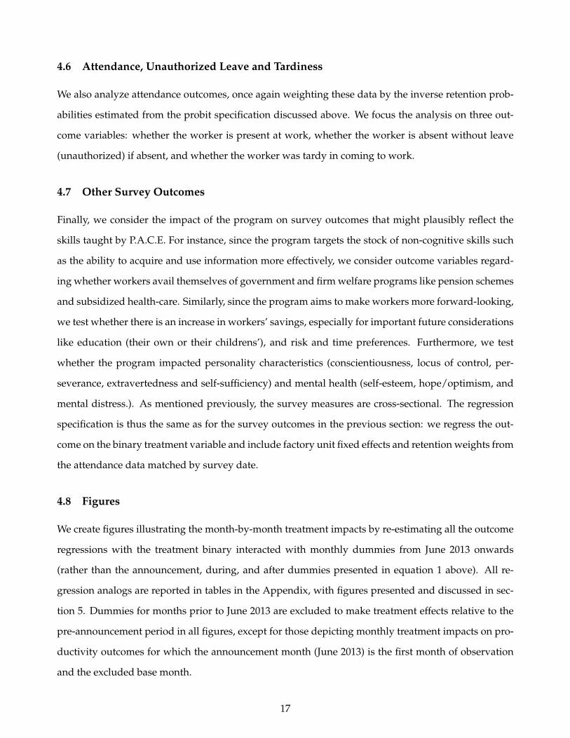
4.6 Attendance, Unauthorized Leave and Tardiness

We also analyze attendance outcomes, once again weighting these data by the inverse retention prob-

abilities estimated from the probit specification discussed above. We focus the analysis on three out-

come variables: whether the worker is present at work, whether the worker is absent without leave

(unauthorized) if absent, and whether the worker was tardy in coming to work.

4.7 Other Survey Outcomes

Finally, we consider the impact of the program on survey outcomes that might plausibly reflect the

skills taught by P.A.C.E. For instance, since the program targets the stock of non-cognitive skills such

as the ability to acquire and use information more effectively, we consider outcome variables regard-

ing whether workers avail themselves of government and firm welfare programs like pension schemes

and subsidized health-care. Similarly, since the program aims to make workers more forward-looking,

we test whether there is an increase in workers’ savings, especially for important future considerations

like education (their own or their childrens’), and risk and time preferences. Furthermore, we test

whether the program impacted personality characteristics (conscientiousness, locus of control, per-

severance, extravertedness and self-sufficiency) and mental health (self-esteem, hope/optimism, and

mental distress.). As mentioned previously, the survey measures are cross-sectional. The regression

specification is thus the same as for the survey outcomes in the previous section: we regress the out-

come on the binary treatment variable and include factory unit fixed effects and retention weights from

the attendance data matched by survey date.

4.8 Figures

We create figures illustrating the month-by-month treatment impacts by re-estimating all the outcome

regressions with the treatment binary interacted with monthly dummies from June 2013 onwards

(rather than the announcement, during, and after dummies presented in equation 1 above). All re-

gression analogs are reported in tables in the Appendix, with figures presented and discussed in sec-

tion 5. Dummies for months prior to June 2013 are excluded to make treatment effects relative to the

pre-announcement period in all figures, except for those depicting monthly treatment impacts on pro-

ductivity outcomes for which the announcement month (June 2013) is the first month of observation

and the excluded base month.

17

4.9 Spillover Effects/Production Complementarity Effects

To estimate the effects on untrained workers who interact with trained workers, we re-run all of the

specifications mentioned above, replacing the binary treatment variable with the binary spillover treat-

ment variable. This variable compares untrained workers in treatment lines (workers who enrolled in

the lottery but did not receive the program and who work in production lines with workers who re-

ceived the training) with control workers in control lines (workers who enrolled in the lottery but did

not receive the program and who work in production lines without any trained workers). Thus, it

takes the value 1 if the individual is an untrained worker in a treated line, and 0 if the worker is a con-

trol worker in a control line. We expect that both due to ease of communication with treated workers

and production complementarities within the line, workers who work alongside treated workers in

the same line are most likely to exhibit externalities to treatment. We supplement this analysis with

partial correlations between productivity measures of workers on the same line in the announcement

month prior to program start. These partial correlations help to indicate the magnitude of the role of

technical complementarities in coincident effects on directly treated and spillover workers.

5 Results

5.1 Retention and Daily Working Status

We begin by measuring the impacts of P.A.C.E. on retention and the probability that a worker is on

the job on a given day. Figure 2A shows raw retention data for both treatment and control groups

over the observation period with training months denoted. The dashed vertical line in Figure 2A

denotes the announcement of assignment to treatment and the vertical solid lines depict the program

window. Since the sampling of retention data started in month 4 of the denoted timeline, retention

is mechanically equal to 1 in the first four months. Figure 2B shows analogous regression coefficients

to those from Table 2, but with treatment effects estimated month by month. This figure shows that

there is a statistically significant impact of treatment on retention early in the program period, which

dissipates by the end of the program (the program training window is denoted by dashed vertical

lines). The figures shown here are from the sample of sewing workers using the attendance data (to

ensure consistency with other outcomes like productivity for which we only have data for the sewing

department). Using the entire sample or the payroll data yields nearly identical figures and so these

18

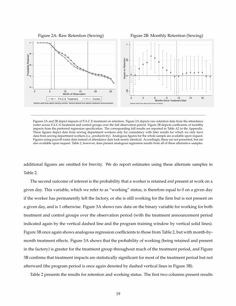
Figure 2A: Raw Retention (Sewing).2

.4.6

.81

Prob

abilit

y Re

tain

ed

0 5 10 15 20 25Month of Observation

P.A.C.E. Treatment ControlVertical solid lines depict training months. Vertical dashed line depicts treatment announcement.

Figure 2B: Monthly Retention (Sewing)

-.05

0.0

5.1

Impa

ct o

n R

eten

tion

0 3 6 9 12 15 18Months Since Treatment Start

Dashed vertical lines depict start and end of training.

Figures 2A and 2B depict impacts of P.A.C.E treatment on retention. Figure 2A depicts raw retention data from the attendanceroster across P.A.C.E treatment and control groups over the full observation period. Figure 2B depicts coefficients of monthlyimpacts from the preferred regression specification. The corresponding full results are reported in Table A2 in the Appendix.These figures depict data from sewing department workers only for consistency with later results for which we only havedata from sewing department workers (i.e., productivity). Analogous figures for the whole sample are available upon request.Figures using payroll roster data instead of attendance data look nearly identical. Accordingly, these are not presented, but arealso available upon request. Table 2, however, does present analogous regression results from all of these alternative samples.

additional figures are omitted for brevity. We do report estimates using these alternate samples in

Table 2.

The second outcome of interest is the probability that a worker is retained and present at work on a

given day. This variable, which we refer to as “working” status, is therefore equal to 0 on a given day

if the worker has permanently left the factory, or she is still working for the firm but is not present on

a given day, and is 1 otherwise. Figure 3A shows raw data on the binary variable for working for both

treatment and control groups over the observation period (with the treatment announcement period

indicated again by the vertical dashed line and the program training window by vertical solid lines).

Figure 3B once again shows analogous regression coefficients to those from Table 2, but with month-by-

month treatment effects. Figure 3A shows that the probability of working (being retained and present

in the factory) is greater for the treatment group throughout much of the treatment period, and Figure

3B confirms that treatment impacts are statistically significant for most of the treatment period but not

afterward (the program period is once again denoted by dashed vertical lines in Figure 3B).

Table 2 presents the results for retention and working status. The first two columns present results

19

Figure 3A: Raw Working (Sewing).2

.4.6

.81

Prob

abilit

y W

orkin

g (R

etai

ned

and

Pres

ent)

0 5 10 15 20 25Month of Observation


Figure 3B: Monthly Working (Sewing)

-.05

0.0

5.1

Impa

ct o

n W

orki

ng



Figures 3A and 3B depict impacts of P.A.C.E treatment on working (retained and present) in the factory. Figure 3A depictsraw presence data from the attendance roster across P.A.C.E treatment and control groups over the full observation period.Figure 3B depicts coefficients of monthly impacts from the preferred regression specification. The corresponding full resultsare reported in Table A2 in the Appendix. These figures depict data from the sample of sewing department workers only, withanalogous whole sample figures showing similar patterns and available upon request

from the attendance data and the third and fourth column from the payroll data. As in the figures,

there is a statistically significant impact of nearly 6 percentage points (pp) during the treatment, and

roughly 4pp when the treatment is announced; the pattern is consistent across both sources of data,

but is statistically stronger when both sewing and non-sewing workers are considered. We conclude

from these results that the program had positive impacts on retention during program announcement

and implementation that are quite large relative to mean retention (nearly 10% of the mean), although

the impacts dissipate after treatment. The results presented in Table A2 in the Appendix (showing im-

pacts for treatment announcement and each month during and after treatment) exhibit a similar pat-

tern - treatment workers are more likely to be retained during the month of treatment announcement

and during treatment, though the impact dissipates towards the end of the program, and disappears

altogether post-treatment.

Table 2 also shows the impacts on the working binary during and after the program. We present the

results from the attendance data for the entire sample and from the production data for the subsam-

ple of sewing department workers. The production data is a precise way to test whether the worker

is actually present on the production line on a given day, and thus a more precise measure of atten-

dance for sewing workers - however, it is only available starting June 2013 (the month of treatment

20

Table 2: Impacts of P.A.C.E. Treatment on Retention and Working Status

(1) (2) (3) (4) (5) (6)

Attendance Roster Production Data

(Whole Sample) (Sewing Dept Only) (Whole Sample) (Sewing Dept Only) (Whole Sample) (Sewing Dept Only)After X P.A.C.E. Treatment 0.0337 0.00534 0.0382 0.00685 0.0170 0.0740**

(0.0230) (0.0257) (0.0265) -0.0274 (0.0190) (0.0364)During X P.A.C.E. Treatment 0.0575** 0.0289 0.0595** 0.0283 0.0431** 0.0897***

(0.0228) (0.0212) (0.0255) (0.0216) (0.0180) (0.0318)Announced X P.A.C.E.. Treatment 0.0406* 0.00416 0.0438* 0.00476 0.0303*

(0.0214) (0.0136) (0.0236) (0.0153) (0.0171)

Fixed EffectsObservations 2,078,400 1,433,981 62,585 43,141 1,848,003 778,916

Control Mean of Dependent Variable 0.589 0.628 0.619 0.656 0.480 0.367

Working1(Worker Retained and Present in

Factory Today)

Notes: Robust standard errors in parentheses (*** p<0.01, ** p<0.05, * p<0.1). Standard errors are clustered at the treatment line level. Retained dummy and Working dummy are both defined for every worker date observation in the data and therfore the regressions do not require any weighting.

Unit X Month X Year, Worker

Retained

1(Worker Still on Payroll Roster)

Retained

1(Worker Still on Attendance Roster)

announcement), and so that month is the excluded category for the productivity data source.

We find that P.A.C.E. treatment affects both outcomes positively (with statistical precision). Treat-

ment workers are about 3pp more likely to be working during treatment than control workers relative

to before treatment, and about 4pp more likely after treatment, a 6-8% increase relative to the mean

probability of working. For the sewing department the impacts relative to the control mean are qual-

itatively similar but larger in magnitude - a 9pp increase during the treatment, and about 7.7pp after

the treatment relative to the treatment assignment announcement period. Appendix Table A2 presents

the results of the regressions that estimate the impact of treatment in each month separately, and as

shown in the Figures 3A and 3B, indicate that the treatment significantly increases the probability that

the worker is retained and present. Thus, the treatment has a strong positive impact on the likelihood

of working.

As discussed in section 4.3 above, impacts on retention and worker presence also have implications

for the estimation of impacts on outcomes that are conditional on being retained or present (e.g., pro-

ductivity and salary). We will therefore use a weighting procedure when measuring impacts on these

outcomes.

21

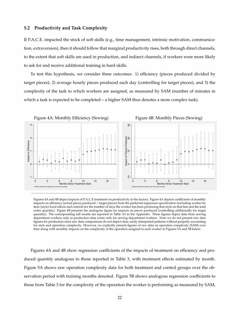
5.2 Productivity and Task Complexity

If P.A.C.E. impacted the stock of soft skills (e.g., time management, intrinsic motivation, communica-

tion, extraversion), then it should follow that marginal productivity rises, both through direct channels,

to the extent that soft skills are used in production, and indirect channels, if workers were more likely

to ask for and receive additional training in hard skills.

To test this hypothesis, we consider three outcomes: 1) efficiency (pieces produced divided by

target pieces); 2) average hourly pieces produced each day (controlling for target pieces); and 3) the

complexity of the task to which workers are assigned, as measured by SAM (number of minutes in

which a task is expected to be completed – a higher SAM thus denotes a more complex task).

Figure 4A: Monthly Efficiency (Sewing)

-.10

.1.2

.3Im

pact

on

Effic

ienc

y



Figure 4B: Monthly Pieces (Sewing)

-10

010

2030

Impa

ct o

n Pi

eces

Pro

duce

d



Figures 4A and 4B depict impacts of P.A.C.E treatment on productivity in the factory. Figure 4A depicts coefficients of monthlyimpacts on efficiency (actual pieces produced / target pieces) from the preferred regression specification (including worker byitem (style) fixed effects and controls for the number of days the worker has been producing that style on that line and the totalorder quantity). Figure 4B presents the analogous figure for impacts on pieces produced (controlling additionally for targetquantity). The corresponding full results are reported in Table A3 in the Appendix. These figures depict data from sewingdepartment workers only as production data exists only for sewing department workers. Note we do not present raw datafigures for production since raw data comparisons do not depict clear, easily interpreted patterns without properly accountingfor style and operation complexity. However, we explicitly present figures of raw data on operation complexity (SAM) overtime along with monthly impacts on the complexity of the operation assigned to each worker in Figures 5A and 5B below.

Figures 4A and 4B show regression coefficients of the impacts of treatment on efficiency and pro-

duced quantity analogous to those reported in Table 3, with treatment effects estimated by month.

Figure 5A shows raw operation complexity data for both treatment and control groups over the ob-

servation period with training months denoted. Figure 5B shows analogous regression coefficients to

those from Table 3 for the complexity of the operation the worker is performing as measured by SAM,

22

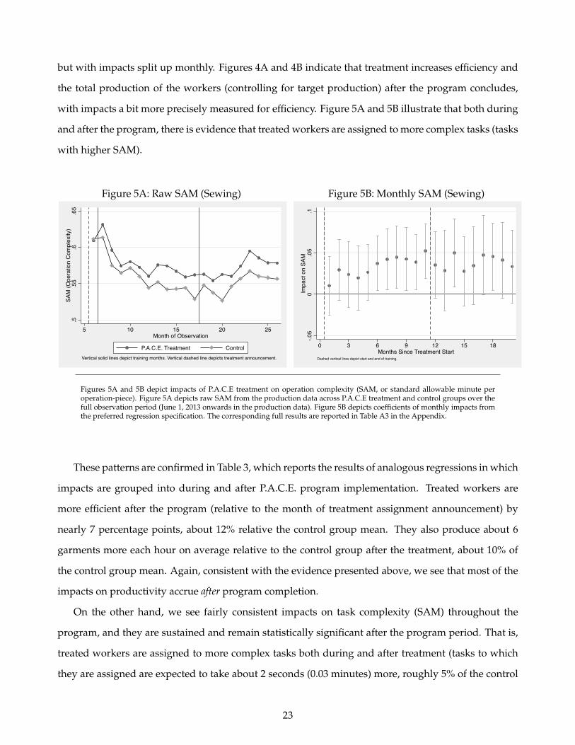
but with impacts split up monthly. Figures 4A and 4B indicate that treatment increases efficiency and

the total production of the workers (controlling for target production) after the program concludes,

with impacts a bit more precisely measured for efficiency. Figure 5A and 5B illustrate that both during

and after the program, there is evidence that treated workers are assigned to more complex tasks (tasks

with higher SAM).

Figure 5A: Raw SAM (Sewing)

.5.5

5.6

.65

SAM

(Ope

ratio

n Co

mpl

exity

)

5 10 15 20 25Month of Observation


Figure 5B: Monthly SAM (Sewing)

-.05

0.0

5.1

Impa

ct o

n SA

M



Figures 5A and 5B depict impacts of P.A.C.E treatment on operation complexity (SAM, or standard allowable minute peroperation-piece). Figure 5A depicts raw SAM from the production data across P.A.C.E treatment and control groups over thefull observation period (June 1, 2013 onwards in the production data). Figure 5B depicts coefficients of monthly impacts fromthe preferred regression specification. The corresponding full results are reported in Table A3 in the Appendix.

These patterns are confirmed in Table 3, which reports the results of analogous regressions in which

impacts are grouped into during and after P.A.C.E. program implementation. Treated workers are

more efficient after the program (relative to the month of treatment assignment announcement) by

nearly 7 percentage points, about 12% relative the control group mean. They also produce about 6

garments more each hour on average relative to the control group after the treatment, about 10% of

the control group mean. Again, consistent with the evidence presented above, we see that most of the

impacts on productivity accrue after program completion.

On the other hand, we see fairly consistent impacts on task complexity (SAM) throughout the

program, and they are sustained and remain statistically significant after the program period. That is,

treated workers are assigned to more complex tasks both during and after treatment (tasks to which

they are assigned are expected to take about 2 seconds (0.03 minutes) more, roughly 5% of the control

23

group mean). Thus, not only are workers in the treatment group assigned to more complex tasks

during and after the program, they are more productive even at these harder tasks once treatment

ends. The non-cognitive skills that the program covers (like time management, goal setting, and team

work) enhance worker productivity and the ability to perform complex tasks.

The time pattern of impacts on productivity – insignificant increases during the program period fol-

lowed by large, significant increases afterward – is striking and deserves additional consideration. We

reason that the “incubation period” for productivity impacts in the context of this program, through

both direct and indirect channels mentioned above, is likely long. First, truly learning soft skills to

the point that they can be applied in the workplace may take time. Second, sets of soft skills may be

complementary, so that the incremental learnings in a given module have a greater impact later in the

program. Third, from anecdotal observation, women took several months to become true participants

in the group sessions; at the beginning of the program the level of participation, fitting with the cultural

context in which these women live, was quite low. Fourth, speaking to the indirect channel of request-

ing and acquiring hard skills, perfecting basic sewing techniques and learning additional ones likely

takes time. Finally, fifth, the more complex tasks to which women were assigned likely generated a lag

in the increase of efficiency.

For all of the above reasons, we might see productivity impacts rising only toward the end of the

program period. We cannot say with statistical power whether the rise in productivity was sudden

(occurring exactly at the end of the program) or more gradual, but the results on quantity, and to a

lesser extent the results on efficiency, seem to indicate a gradual pattern that begins several months

before program completion.

5.3 Person Days and Career Advancement

In addition to worker presence and productivity, we consider the total number of working days ac-

crued to the firm, and career advancement within the firm. The measure of the first outcome is the

cumulative number of working days that accrue to the firm. This is the running sum of the worker

presence, which is the cumulative number of days that the worker was present in the firm. Since this

variable is not conditional on retention (not missing if the worker has left the firm), no re-weighting

of the treatment and control groups are required. To estimate the impacts of treatment on career ad-

vancement, we consider both whether the worker was given a raise using monthly payroll data as

24

Table 3: Impacts of P.A.C.E. Treatment on Productivity

(1) (2) (3)Efficiency Pieces Produced SAM (Operation Complexity)

Mean(Produced/Target) Mean(Pieces per Hour) Mean(Standard Allowable Minute)

After X P.A.C.E. Treatment 0.0681** 7.272** 0.0334*

(0.0301) (3.286) (0.0180)

During X P.A.C.E. Treatment 0.0203 1.926 0.0320**

(0.0153) (1.812) (0.0146)

Additional ControlsDays on Same Line-Garment, Total

Order Size

Days on Same Line-Garment, Total

Order Size, Target PiecesNone

Fixed Effects Unit X Month X Year, Worker

Weights

Observations 290,763 290,763 290,763

Control Mean of Dependent Variable 0.542 62.250 0.565

Inverse Predicted Probability from Probit of Working on Treatments X Mo-Yr X Baseline Characteristics

Notes: Robust standard errors in parentheses (*** p<0.01, ** p<0.05, * p<0.1). Standard errors are clustered at the treatment line level. Observations are weighted in regressions by the inverse of the predicted

probability of working (i.e., not yet attrited and present in the factory with non-missing data) in the sample that day from a probit regression of the working dummy on month by year FE and their

interaction with individual and line treatment dummies and baseline variables reported in Table 1. Sample is trimmed in these regressions to omit days in which the worker is observed for only a half a

production day or less or days in which the worker is observed for more than 2 overtime hours as these are anomalous observations with imprecise production measures. These outliers make up only

around 5% of the work-day observations

Unit X Month X Year, Worker X Garment

well as worker-reported measures of expectations of promotion, whether they recently asked for (and

received) skill development training and production incentives, and finally, how they assess their own

ability relative to all workers on their production line, and relative to workers in their production line

that are the same skill level as them. Except for the salary data which is at the monthly level for each

worker, the self-reported measures are from a worker-level survey and vary only cross-sectionally.

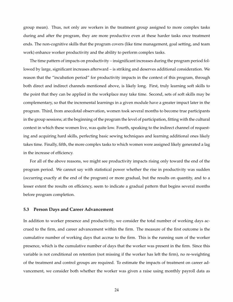
Figures 6A and 6B show that the treatment impact on cumulative person days is positive and statis-

tically significant by roughly 3 months into the program period. The impacts continue to grow quickly

through month 8 of the training period, after which the growth slows somewhat but remains positive

through the remainder of the observation period. Columns 1 and 2 of Table 4 show the impacts on

cumulative person days during and after the program, using attendance and production data, respec-

tively. We present the results from the attendance data for the entire sample and from the production

data for the subsample of sewing department workers. The treatment increases the cumulative person

days per treated worker by 8.5 days during treatment and 19 days after treatment when the entire

sample is considered, which is about 4.25% and 9% of the mean cumulative number of days of the

control group.

Appendix Table A4 presents the results of the regressions that estimate the impact of treatment in

each month separately, and as shown in the Figures 6A and 6B, indicate that the treatment significantly

increases the cumulative person days during and after the program. Thus, the treatment has a strong

25

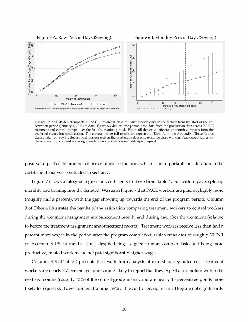
Figure 6A: Raw Person Days (Sewing)0

5010

015

020

0Cu

mul

ative

Per

son

Days

(Day

s W

orke

d to

Dat

e)

5 10 15 20 25Month of Observation


Figure 6B: Monthly Person Days (Sewing)

010

2030

40Im

pact

on

Cum

ulat

iveM

anD

ays



Figures 6A and 6B depict impacts of P.A.C.E treatment on cumulative person days in the factory from the start of the ob-servation period (January 1, 2013) to date. Figure 6A depicts raw person days data from the production data across P.A.C.Etreatment and control groups over the full observation period. Figure 6B depicts coefficients of monthly impacts from thepreferred regression specification. The corresponding full results are reported in Table A4 in the Appendix. These figuresdepict data from sewing department workers only as the production data only exists for these workers. Analogous figures forthe whole sample of workers using attendance roster data are available upon request.

positive impact of the number of person days for the firm, which is an important consideration in the

cost-benefit analysis conducted in section 7.

Figure 7 shows analogous regression coefficients to those from Table 4, but with impacts split up

monthly and training months denoted. We see in Figure 7 that PACE workers are paid negligibly more

(roughly half a percent), with the gap showing up towards the end of the program period. Column

3 of Table 4 illustrates the results of the estimation comparing treatment workers to control workers

during the treatment assignment announcement month, and during and after the treatment (relative

to before the treatment assignment announcement month). Treatment workers receive less than half a

percent more wages in the period after the program completion, which translates to roughly 30 INR

or less than .5 USD a month. Thus, despite being assigned to more complex tasks and being more

productive, treated workers are not paid significantly higher wages.

Columns 4-8 of Table 4 presents the results from analysis of related survey outcomes. Treatment

workers are nearly 7.7 percentage points more likely to report that they expect a promotion within the

next six months (roughly 13% of the control group mean), and are nearly 15 percentage points more

likely to request skill development training (59% of the control group mean). They are not significantly

26

Figure 7: Monthly Salary (Sewing)

0.0

05.0

1.0

15Im

pact

on

log(

Gro

ss S

alar

y)



Figure 7 depicts coefficients of monthly impacts of P.A.C.E treatmenton log(gross salary) from the preferred regression specification. Thisfigure depicts data for sewing department workers only as aforemen-tioned productivity impacts and profitability calculations discussedbelow pertain only to this sample. The corresponding full results areavailable upon request.

more likely to report having received a production incentive or award, but rate themselves higher rel-

ative to relative to all co-workers in their production line. Specifically, when asked to rank themselves

relative to workers in their production line of the same skill grade level, they are significantly more

likely to rate themselves at a higher level (as shown in column 8). Finally, Table A4 in the Appendix

presents the month by month estimation results for cumulative person days and salary. As shown in

the figures, salaries are marginally higher for treatment workers in the last 2 months of treatment and

after program completion.

5.4 Attendance

Related outcomes of interest are attendance (a binary variable that is 1 if the worker is at work today

and 0 if not), unauthorized leave (a binary variable that is 1 if the worker is not at work today and

did not inform the employer and 0 if she is either at work or absent and took prior formal leave from

the employer), and tardiness (a binary variable that is 1 if the worker was late relative to the modal

arrival time of co-workers on the line that day and 0 if not). Appendix Table A5 present the impacts of

treatment on these outcomes. There are no precisely measured impacts on any of the outcomes if the

grouping is done by these milestones rather than a month by month comparison. Appendix Table A6

27

Table 4: Impacts of P.A.C.E. Treatment on Cumulative Person Days and Career Advancement

(1) (2) (3) (4) (5) (6) (7) (8)

log(Gross Salary)Expect

Promotion Next 6 Mos

Skill Development

Training

Production Award or Incentive

Line Co-Worker Self-Assessment

Skill Peer Self-Assessment

Attendance Roster Production Data Salary Data

(Whole Sample) (Sewing Dept Only) (Sewing Dept Only)

After X P.A.C.E. Treatment 19.44** 15.74** 0.00493*(8.495) (6.888) (0.00274)

During X P.A.C.E. Treatment 8.410* 6.339*** 0.00114(4.281) (2.393) (0.000835)

Announced X P.A.C.E. Treatment -1.058 0.000218(4.938) (0.000648)

P.A.C.E. Treatment 0.0767* 0.148*** 0.0281 0.0784 0.130**(0.0429) (0.0484) (0.0184) (0.0688) (0.0645)

Fixed Effects

Weights

Observations 1,848,003 778,916 28,692 621 621 621 621 621Control Mean of Dependent

Variable 201.408 103.220 8.909 0.562 0.251 0.032 5.276 5.321

Inverse Predicted Probability from Probit of Retention on Treatments X Mo-Yr X Baseline Characteristics

Notes: Robust standard errors in parentheses (*** p<0.01, ** p<0.05, * p<0.1). Standard errors are clustered at the line level. Observations are weighted in regressions by the inverse of the predicted probability of being retained (i.e., not yet attrited with non-missing data) in the sample that day from a probit regression of the retained dummy on month by year FE and their interaction with individual and line treatment dummies and baseline variables reported in Table 1.

Unit

Survey Data

Self-Reported Binary from Survey

Cumulative Person Days

Sum of Days Working for Each Worker to Date

None


(Sewing Dept Only)

28

presents the regression results of the month by month estimation. The results indicate that treatment

workers are more likely to attend work in the first two months of the program, and absences are more

likely to be authorized during the same months. Worker tardiness does not appear to be impacted

during or after treatment.

6 Mechanisms

Our interpretation of the results presented in the previous section is that skills like time and stress man-

agement; communication; problem solving and decision-making; and effective teamwork are “soft”

inputs into production. Reinforcing these skills through the P.A.C.E. program should thus directly af-

fect workplace outcomes. Across the categories of results presented below, impacts are consistent with

a direct treatment effect on the stock of soft skills. In particular, the narrative that emerges is one that

is consistent with the P.A.C.E. program creating more “empowered” women. That is, women who are

more extraverted; more likely to seek out and avail themselves of government and employer benefits

to which they are entitled; more likely to proactively increase their stock of hard skills by requesting

technical training; and more likely to exhibit forward looking behavior via savings and aspirations for

their children’s future. Finally, these women share learnings with their co-workers, and these spillovers

contribute to more productive co-workers over and above direct production complementarities.

Below, we argue for this interpretation using evidence from a survey of treatment and control

workers; from assessments of the treatment group’s knowledge before and after the completion of the

program’s core modules; and from the size and nature of treatment spillovers. We also present several

alternative interpretations and discuss the plausibility of each in turn.

6.1 Survey Results

The first piece of evidence supporting the interpretation that the stock of soft skills changed comes

from a survey we administered to treatment and control workers in the month after program comple-

tion. Table 5 evaluates the impact of P.A.C.E. treatment on financial behaviors and attitudes (Panel A);

availing of firm and government programs (Panel B); personality (Panel C); and mental well-being and

aspirations (Panel D).

We discuss results in support of each category in turn to lay out our reasoning. The first category

is meant to evaluate whether P.A.C.E. treatment changes women’s financial behaviors and attitudes.

29

Table 5: Impacts of P.A.C.E. Treatment on Women’s Outcomes

(1) (2) (3) (4) (5)

Panel A: Financial Behaviors and AttitudesSaving for Education

Saving for Other Reasons

Risk and Time Preference Index

InsuranceInformal Borrow or

Lend

P.A.C.E. Treatment 0.0607* -0.0332 -0.154* 0.00742 0.0235(0.0349) (0.0364) (0.0866) (0.0395) (0.0444)

Control Group Mean of Dependent Variable 0.263 0.273 0.054 0.368 0.429

Panel B: Government and Firm Entitlements Gov. PensionGov. Subsidized

HealthcareOther Gov.

SubsidyFirm Entitlements

Community Self Help Group

P.A.C.E. Treatment 0.0232* 0.0221** 0.00746 -0.0303 -0.0346(0.0137) (0.00982) (0.0299) (0.0332) (0.0313)


Panel C: Personality Conscientiousness Locus of Control Perserverance Extravertedness Self-Sufficiency

P.A.C.E. Treatment 0.0530 0.0264 -0.105 0.159** 0.0383(0.0776) (0.0787) (0.0902) (0.0678) (0.0872)

Control Group Mean of Dependent Variable -0.041 -0.023 0.037 -0.064 -0.067

Panel D: Mental Health and Aspirations Self-Esteem Hope/Optimism Moderate DistressChild's Expected Age at Marriage

Child Educated Beyond College

P.A.C.E. Treatment -0.158 -0.0634 -0.0419 0.0793 0.0808***(0.113) (0.0837) (0.0384) (0.167) (0.0280)


Fixed Effects Unit Unit Unit Unit UnitWeighted Yes Yes Yes Yes Yes

Observations 621 621 621 621 621

Notes: Robust standard errors in parentheses (*** p<0.01, ** p<0.05, * p<0.1). Standard errors are clustered at the treatment line level. Obersvations are weighted in regressions by the inverse of the predicted probability of being retained (i.e., not yet attrited with non-missing data) in the sample that day from a probit regression in the attendance roster of the retained dummy on month by year FE and their interaction with individual and line treatment dummies and baseline variables reported in Table 1.

30

This change would be consistent with a shift in forward-looking behavior, an important dimension

of soft skills. The results from Panel A indicate that there is a positive impact on saving for own and

children’s education, and the impacts are quite large relative to the control group mean (about a quar-

ter of the control group mean). Savings for other purposes show no significant impacts; self-reported

measures of participating in insurance and informal lending show positive but insignificant impacts.

Finally, we construct a survey-based measure of combined risk-aversion and patience with higher

scores corresponding to extreme, seemingly irrational, levels of risk aversion and patience (i.e., domi-

nated selections between tradeoffs of certain and risky payouts and current and future payouts). The

estimate suggests that treatment reduces this baseline extreme risk aversion and patience, although

this estimate is measured imprecisely.

The second category, availing oneself of government and employer-based entitlement programs,

is meant to evaluate changes in the effectiveness of information acquisition, another important soft

skill. The results in Panel B show that treated workers are substantially more likely to seek out welfare

programs. Impacts on binary indicators for self-reported seeking out of government pension and

government subsidized healthcare indicate that treated workers are more likely to avail themselves

of these programs. The magnitude of these impacts are quite large relative to control group means,

which are around 0 for both outcomes. Impacts on other government subsidies and firm entitlements

are negligible. Finally, we find the intriguing result that membership in community self-help groups

(a common and often powerful feature of social networks for Indian women) goes down, though this

estimate is imprecise. This result might suggest a substitution occurring due to the P.A.C.E. program’s

impact on social connections and empowerment-related agenda in the workplace.

The third category, personality, is meant to assess differences in key traits that are associated with

the stock of soft skills, namely conscientiousness, locus of control, perseverance, extraversion, and

self-sufficiency. In general, the impact estimates (shown in Panel C) suffer from lack of precision,

but P.A.C.E. treatment does have a large positive and statistically significant impact on extraversion.

This result on extraversion is consistent with the results above related to seeking out information and

resources, as well as results on self-reported comparisons to co-workers, which show that P.A.C.E.

training increased self-regard with respect to workplace performance relative to peers.

The final category of the survey, mental health and aspirations, is meant to assess impacts on psy-

chological well-being and the extent to which future aspirations are affected by treatment. The results

reported in Panel D show that, in general, outcomes associated with psychological well-being (self-

31

esteem, optimism, and mental distress) are unaffected by P.A.C.E. treatment, but aspirations for chil-

dren’s education rise dramatically in relation to the control group mean. This is consistent with the

result on saving for education presented in Panel A.

6.2 Pre- and Post-Module Assessments

Figure 8A: Post - Pre % Change in Score

34

56

7Pe

rcen

t Cha

nge

in T

est S

core

Com

mun

icat

ion

Prob

lem

-Sol

ving

/Dec

isio

n-M

akin

g

Tim

e &

Stre

ss M

anag

emen

t

Fina

ncia

l Lite

racy

Hea

lth

Lega

l Lite

racy

Exec

utio

n Ex

celle

nce

Figure 8B: Post - Pre Difference in Score

.8.9

11.

11.

2D

iffer

ence

in T

est S

core

Com

mun

icat

ion

Prob

lem

-Sol

ving

/Dec

isio

n-M

akin

g

Tim

e &

Stre

ss M

anag

emen

t

Fina

ncia

l Lite

racy

Hea

lth

Lega

l Lite

racy

Exec

utio

n Ex

celle

nce

Figures 8A and 8B depict normalized (percent change, 8A) and raw (8B) differences in the pre- and post-module assessmentsadministered for all core P.A.C.E. modules. Raw scores for each assessment are out of 100. These assessments were, of course,not given to control workers and accordingly cannot be analyzed in the preferred specification.

The second source of evidence on the direct impacts of P.A.C.E. on the stock of soft skills is pre- and

post-module assessments built into the program. These assessments were designed to test the specific

value added from each core program module. They were only administered to program participants,

and thus we cannot compute a treatment v. control difference, rather only a post- v. pre-module

difference.

We present two sets of results, shown in Figures 8A and 8B. Figure 8A shows the difference between

(identical) assessments taken pre- and post-module completion normalized by the baseline score, cre-

ating a percent change indicator from pre to post for each core P.A.C.E. module. Figure 8B shows the

raw difference between the pre- and post-module assessments, again for the set of core modules.

The results from both analyses show that P.A.C.E. participants retained, and were able to commu-

nicate, the soft skills acquired in each of the program’s core modules. The changes shown in Figure 8A

32

are all in the neighborhood of 5-6 percent, with the largest impacts (in percent terms) for Communi-

cation, Execution Excellence, Legal Literacy, and Problem-solving/Decision-making.. The largest raw

difference, shown in Figure 8B, is from the Communication module.

These results fit well with the notion that workers absorbed the skills taught in each of the core

modules, and that the stock of skills increased, at least in the short run. There are several caveats in

interpreting these changes. First, as described above, control workers were not given the assessments,

so we are not able to estimate impacts by comparing across randomized participants (treatment v.

control). Second, we are measuring skill retention directly after module completion; this does not

necessarily reflect true (long-term) skill absorption. Nevertheless, these assessments offer some sup-

porting evidence that is consistent with our hypothesis that P.A.C.E. acted on workplace outcomes by

increasing the stock of soft skills.

6.3 Treatment Spillovers

Finally, we consider evidence on spillovers. Recall that the experiment was designed to capture

spillovers within production lines through a two-stage randomization procedure, in which lines were

first randomized to treatment or control, and then within treatment lines, workers who had enrolled in

the P.A.C.E. lottery were randomized to treatment or to the spillover group. In this section we evaluate

spillovers by comparing the outcomes of this latter group to control workers on control lines.

Spillovers are important from both a program evaluation standpoint as well as from the perspec-

tive of understanding mechanisms of impact. Regarding program evaluation, if spillovers are large,

then we know the program’s benefits extend to non-participants through communication amongst

co-workers, providing greater justification for employer investment in soft skills training. Regarding

mechanisms, if spillovers exist, we know that it is likely that participants actually increased their stock

of soft skills enough to share some of those gains with their co-workers. We evaluate these hypotheses

in Table 6, which presents the spillover results for workplace outcomes of interest. (Note that probabil-

ity weights, when necessary, are calculated exactly as they are in the treatment effect estimation, using

spillover treatment indicators in place of direct P.A.C.E. training.)

Panel A presents the results for person days as well as productivity and task complexity. There are

some weakly statistically significant impacts on the binary for working during treatment for the entire

sample, and a stronger result for cumulative person days - untrained workers who work with treated

33

Table 6: Spillovers on Co-Workers (Attendance, Productivity, and Career Advancement)

(1) (2) (3) (4) (5) (6) (7)

Attendance Production Attendance Production

After X Spillover -0.0163 0.0350 8.867 8.034 0.0648* 7.383* 0.0396**(0.0207) (0.0434) (9.079) (7.626) (0.0349) (3.812) (0.0174)

During X Spillover 0.0297 0.0663* 7.780** 4.489 0.00787 1.072 0.0111(0.0211) (0.0385) (3.568) (2.820) (0.0162) (2.137) (0.0132)

Announced X Spillover 0.0317* 2.151(0.0172) (1.372)

Fixed EffectsUnit X Month X

Year, Worker

Weights

Observations 1,102,880 673,407 562,478 673,407 241,322 241,322 241,322Control Mean of Dependent Variable 0.519 0.382 0.390 107.437 0.548 63.011 0.565

Panel B: Retention and Career Advancement log(Gross Salary)Skill Development

TrainingProduction Award or

IncentiveLine Co-Worker Self-

AssessmentSkill Peer Self-

Assessment

Attendance Payroll

After X Spillover -0.0177 -0.0155 0.00907***(0.0246) (0.0257) (0.00300)

During X Spillover 0.0361 0.0386 0.00198**(0.0234) (0.0239) (0.000813)

Announced X Spillover 0.0173 0.0197 0.000313(0.0161) (0.0177) (0.000544)

Spillover 0.0168 0.0116 0.132* 0.0933(0.0584) (0.0226) (0.0717) (0.0704)

Fixed Effects

Weights

Observations 1,241,328 37,357 24,508 527 527 527 527Control Mean of Dependent Variable 0.628 0.656 8.909 0.247 0.030 5.243 5.270

Notes: Robust standard errors in parentheses (*** p<0.01, ** p<0.05, * p<0.1). Standard errors are clustered at the treatment line level. All regressions are for sewing department workers only as spillover sample is not defined for non-sewing workers. Retained and working dummies and cumulative man days are defined for every worker date observation in the data and therfore regressions do not require any weighting. Observations in attendance and advancement regressions are weighted in regressions by the inverse of the predicted probability of being retained (i.e., not yet attrited with non-missing data) in the sample that day from a probit regression of the retained dummy on month by year FE and their interaction with individual and line treatment dummies and baseline variables reported in Table 1.

Retained

Inverse Predicted Probability from Probit of Retention on Treatments X Mo-Yr X Baseline CharacteristicsNone


NoneInverse Predicted Probability from Probit of Working on

Treatments X Mo-Yr X Baseline Characteristics

SAM (Operation Complexity)

Unit X Month X Year, Worker Unit X Month X Year, Worker X Garment

Panel A: ProductionWorking Cumulative Man Days

Efficiency Pieces Produced

workers work for about 7.8 more days during program months relative to control workers. Moreover,

efficiency, pieces produced, and SAM show spillover impacts nearly as large as the main impacts of

P.A.C.E. treatment. Panel B presents the results for career advancement variables. As in the productiv-

ity and task complexity outcomes, the spillover impacts on salary are of the same magnitude as direct

effects (though more precisely estimated). We interpret wage impacts on spillovers as precisely esti-

mated 0s (point estimates indicate raises of less than 1%). The worker survey outcomes on expected

probability of promotion, requesting skill development training, receiving a production incentive or

self-assessment relative to co-workers are not precisely measured, but again have coefficients of the

same sign as the main treatment impacts.

Table 7 presents the results for the non-workplace outcomes of interest for spillovers. The only

34

strongly statistically significant impacts are that workers who work with treated workers are more

likely to avail of government subsidized healthcare. On the whole, impacts on non-workplace out-

comes do not show any robust spillover impacts.

In sum, then, for workplace outcomes we see large spillover impacts on cumulative person days

accrued to the firm, efficiency and pieces produced and task complexity, with many of these impacts

being nearly as large as those from direct training. We see some evidence for spillovers on outcomes

outside the workplace, but the results are imprecise in general. Overall, the presence of spillovers

suggests that knowledge transfer happened as a direct result of the program – i.e., that program par-

ticipants imbibed soft skills, which they then communicated to co-workers on their production lines,

and that transfer helped improve outcomes of non-participants, as well.

It should be noted that it is possible that spillover impacts are observed in our setting, even ab-

sent any true transfer of soft skills, by way of technical complementarities in production. While these

certainly exist given the team production environment in our context, we do not think the evidence

supports the hypothesis that spillovers are entirely, or even mostly, due to technical complementarity.

We estimate partial correlations between contemporaneous productivity measures of co-workers on

the line using pre-program data (during the announcement month of June 2013) and find that the size

of the complementarities are substantially smaller than the spillover effect estimates on productivity

presented here. According to our estimates, technical complementarities produce partial correlations

of less than 30% in within line efficiency across co-workers, roughly 20% in pieces produced contem-

poraneously by co-workers, and less than 5% in complexity of task assignments within garment style.

See Appendix section A.3 for more detail on the estimation of complementarities.

6.4 Alternate Mechanisms

Having presented evidence on the salience of direct skilling as a result of the P.A.C.E. program, we

now discuss several alternative interpretations of the results and any supporting evidence of each.

First, we evaluate the possibility that the effects were due to sheepskin effects i.e. taking part in

P.A.C.E. “certified” workers as high quality from the perspective of management, and this led to the

improvements in workplace outcomes we observe. We reason that sheepskin effects are unlikely to

explain the majority of the program’s impacts given the presence of large spillovers. That is, non-

participants (who should have no gains through sheepskin effects) who worked with P.A.C.E.-trained

35

Table 7: Spillovers on Co-Workers (Financial Behaviors, Personality, and Mental Health)

(1) (2) (3) (4) (5)

Panel A: Financial Behaviors and AttitudesSaving for Education



InsuranceInformal Borrow or

Lend

Spillover 0.0547 0.00840 -0.111 0.0428 -0.0320(0.0419) (0.0431) (0.106) (0.0469) (0.0470)


Panel B: Government and Firm Entitlements Gov. PensionGov. Subsidized




Spillover 0.0107 0.0327** 0.0213 -0.0166 0.0114(0.0178) (0.0142) (0.0320) (0.0238) (0.0323)


Panel C: Personality Conscientiousness Locus of Control Perserverance Extravertedness Self-Sufficiency

Spillover -0.00153 0.122 -0.152 0.0903 0.0861(0.0838) (0.0889) (0.0958) (0.0863) (0.0979)

Control Group Mean of Dependent Variable -0.027 -0.044 0.033 -0.079 -0.056

Panel D: Mental Health and Aspirations Self-Esteem Hope/Optimism Moderate DistressChild's Expected Age at Marriage


Spillover -0.169* -0.0949 -0.00407 -0.0830 0.0399(0.0974) (0.0956) (0.0311) (0.210) (0.0335)


Fixed Effects Unit Unit Unit Unit UnitWeighted Yes Yes Yes Yes Yes

Observations 527 527 527 527 527

Notes: Robust standard errors in parentheses (*** p<0.01, ** p<0.05, * p<0.1). Standard errors are clustered at the treatment line level. Observations are weighted in regressions by the inverse of the predicted probability of being retained (i.e., not yet attrited with non-missing data) in the sample that day from a probit regression in the attendance roster of the retained dummy on month by year FE and their interaction with individual and line treatment dummies and baseline variables reported in Table 1.

36

workers showed large impacts on workplace outcomes.

Second, we evaluate reciprocity (an impulse to give back to the employer as a result of access to the

program) as the predominant mechanism driving workplace impacts. While it is plausible that some

part of the impacts observed is due to reciprocity, we find it unlikely that the majority of impacts are

due to this mechanism. This is for two reasons. First, again, spillovers in treatment would be difficult

to explain if reciprocity were the main driving force behind workplace impacts, since non-participants

should not be driven by this motive. Second, productivity impacts accumulate slowly during the pro-

gram period and persist for at least 9 months after program completion, with the largest productivity

impacts occurring during this post-training period. This does not fit well with a reciprocity motive

as a primary mechanism, since we would expect the reciprocity motive to be strongest while the pro-

gram is offered. This is in line with recent evidence on the limited role for reciprocity in the workplace

(DellaVigna et al., 2016).

Finally, we evaluate the idea that increased social capital drives the results on workplace impacts.

The argument here is that it is possible that P.A.C.E. group sessions encouraged social interaction,

which in turn has productive benefits through knowledge and skill transfer. Indeed, recent work by

Menzel (2015), who carried out an experiment shifting the extent of social connectivity in garment

factories in Bangladesh, affirms this idea.

While it is quite likely (from casual observation of the program sessions) that P.A.C.E. did increase

social capital among workers, we contend that it probably did not account for the majority of program

impacts. First, language-based and cultural barriers are quite salient in the workplace in our context,

likely limiting the extent of the importance of social connectivity in productivity. Nearly half the work-

ers in the factories under study are migrants, many of whom do not speak Kannada, the indigenous

language of Karnataka (the Indian state where Bengaluru is located). Second, due to throughput con-

straints which dictated the number of workers from the same production line who could leave at the

same time for a P.A.C.E. session, co-workers on the same line were usually placed in different sessions.

Again, this likely limited the increase in within-line social connectivity. These explanations do not

preclude social ties from being a salient mechanism; they simply lower the likelihood that this channel

generated workplace impacts.

37

7 Conclusion

In this paper, we evaluate the workplace impacts of general training in soft skills development. Con-

sistent with theories of labor market imperfections and firms’ gains from general training, we find that

workers are substantially more productive after soft skills training, and that treated workers are no

more likely to leave after training than controls. Wages rise by a very small amount after the program

period, suggesting that the firm captures most of the gains from the increased marginal productivity of

labor.

Figure 8: Total Program Costs Over Time

020

4060

8010

0N

PV o

f Pro

gram

Cos

t (Th

ousa

nds

USD

)


Trainer Salary Costs Lost Man Hours CostsTotal Costs


To quantify the total returns in terms of profit to the firm, we combine our treatment effect es-

timates on retention (person-days) and productivity with costing data obtained from the program

administrators. We report in Table 8 calculations of the net-present-value costs and benefits. Benefits

are calculated in terms of additional person days and incremental productivity from treated workers

using estimates from the randomized evaluation.17 We ignore spillover impacts and focus on direct

treatment benefits only. This is primarily because the costs and benefits for individual trainees scale

17We ignore wage increases in these calculations as treatment impacts on salaries were negligible. In addition, we implicitlyassume in calculating lost productivity due to reduced person days that the rate of hiring or worker replacement is commonacross treatment and control workers such that differential attrition produces truly lost person days. This is largely trueas hiring is centralized for each factory unit, and even across factories with respect to migrant workers and new trainees.Accordingly, we are told that it is impossible for the rate of recruitment, hiring, and training to respond to differentialturnover across lines within a factory and even to a degree across factories.

38

linearly, while spillover impacts are likely non-linear in the proportion of a line treated. (In addition to

this, production complementarities are also likely non-linear and more salient when a larger fraction

of the line is treated.) For this reason, to remain as conservative regarding benefits of the program as

possible, we omit spillover impacts from the calculations that follow.

Figure 9: Cumulative Program Benefits Over Time0

100

200

300

NPV

of P

rogr

am B

enefi

ts (T

hous

ands

USD

)


Total Costs Additional Man DaysAdditional Productivity Total Benefits


Table 8 first outlines costs of the program, both overhead costs and variable costs. The overhead

costs are given entirely by the costs of hiring two full-time trainers per factory for the 11 months

of the program. The variable costs are from lost production hours. For the 1,087 treated workers,

total program costs are approximately $90,285, about $30,000 of which are overhead costs, and the

remainder variable costs associated with lost hours. The time path of total costs in net present value

(NPV) are shown in Figure 8. This figure shows that both components of total costs rise linearly during

the program period, peaking at program completion.

Details on profit margins on additional revenue both from an additional person day and additional

productivity, as well as additional revenue per garment were obtained from the firm. The benefits

of the program accrue from the higher number of cumulative person days accrued to the firm and

higher productivity. At the end of the program period, the NPV of these benefits is just over $100,000,

about three-quarters of which is the result of person days gained due to differential attrition during

the program. At the end of our tracking period (9 months after program completion), total benefits are

39

Table 8: Return on Investment Calculations (Costs and Benefits to Firm)

Sewing Department Only (1087 Treated Workers) P.A.C.E. Training Overhead Cost (2 Trainers per Factory for 11 Mos) -$30,065.26 P.A.C.E. Training Variable Cost (Lost Garments from Lost Man Hours) -$60,219.47Total Cost (All numbers in present value) -$90,284.73

1 Year After Program Announcement Additional Man Days $76,308.65 Additional Productivity $25,095.73 Net Present Value of Subtotal $101,404.40 Net Rate of Return 12%

20 Mos After Program Announcement Additional Man Days (End of Observation) $104,520.70 Additional Productivity (Garments per 8 hr day) $216,767.10 Net Present Value of Subtotal $321,287.80 Net Rate of Return 256%

Assumptions Additional Garments per Additional Man Day 8.3 Additional Revenue per Garment $7.00 Labor Contribution to Cost ("Cut to Make") 30% Profit Margin on Additional Revenue from Additional Productivity 24% Profit Margin on Additional Revenue from Additional Man Day 6% Interest Rate 7.5% INR per 1 USD 60

Table 8Return on Investment Calculations

Notes: Trainer salaries were 17,000 INR per year for each trainer. There were 2 trainers for each of the 5 factories; 10 trainers in total. Additional garments per additional man day is calculated by dividing the average worker level SAM (minutes to complete the operation on a single garment) by the line level SAM (minutes to complete a full garment for the line) and multiplying by 480 minutes in a work day. Additional revenue per garment is taken from the accounting department of the firm, as is the "Cut to Make" or labor percent contribution to total production cost. Profit margin on additional revenue generated through improved efficiency is calculated as 80% of the "Cut to Make" cost as instructed by the accounting office of the firm and the profit margin on additional revenue from an additional man day is equivalent to the average profit margin of the firm. The monthly interest rate is the average interest rate that prevailed during the study time period. Similarly, the exchange rate is the average from the study period.

40

substantially higher, more than $320,000. In the post-program period, returns via productivity gains

dominate, accounting for more than two-thirds of the total benefits. Figure 9 plots the time path of

cumulative benefits to the firm. Note that these returns accrued net of attrition – that is, we only count

person days gained and productivity increases accruing to workers who were still present at each point

in time.

Figure 10: Cumulative and Flow Return Over Time

-10

12

3M

onth

ly F

low

Gai

n in

Pro

fits

(%)

050

100

150

200

250

Ret

urn

on In

vest

men

t (%

)


Cumulative RoI (NPV) Monthly Flow Profit GainDashed vertical lines depict start and end of training.

The net rate of return at the end of the program period is thus 12%. That is, by the time the program

ended, program costs had been recouped by the firm, plus 12 percent additional returns. Twenty

months after program completion, flow benefits from post-program productivity impacts help gener-

ate a net rate of return of 256%. Figure 10 shows the time path of the cumulative and flow net rate of

return. As depicted by the dashed line corresponding to the right axis, flow returns are roughly 2% at

the end of the observation period, indicating that this cumulative return of 256% will likely continue

to grow.

41

References

Acemoglu, D. (1997). Training and innovation in an imperfect labour market. The Review of Economic

Studies, 64(3):445–464.

Acemoglu, D. and Pischke, J.-S. (1998). Why do firms train? theory and evidence. The Quarterly Journal

of Economics, 113(1):79–119.

Acemoglu, D. and Pischke, J.-S. (1999). Beyond becker: training in imperfect labour markets. The

Economic Journal, 109(453):112–142.

Afridi, F., Dinkelman, T., and Mahajan, K. (2016). Why are fewer married women joining the work

force in india? a decomposition analysis over two decades.

Aizer, A. and Cunha, F. (2012). The production of child human capital: Endowments, investments and

fertility. Unpublished paper, Brown University.

Altonji, J. G. and Spletzer, J. R. (1991). Worker characteristics, job characteristics, and the receipt of

on-the-job training. Industrial & Labor Relations Review, 45(1):58–79.

Anderson, M. L. (2008). Multiple inference and gender differences in the effects of early intervention: A

reevaluation of the abecedarian, perry preschool, and early training projects. Journal of the American

Statistical Association, pages 1481–1495.

Attanasio, O. P., Fernandez, C., Fitzsimons, E. O., Grantham-McGregor, S. M., Meghir, C., and Rubio-

Codina, M. (2014). Using the infrastructure of a conditional cash transfer program to deliver a

scalable integrated early child development program in colombia: cluster randomized controlled

trial. BMJ, 349:g5785.

Autor, D. H. (2001). Why do temporary help firms provide free general skills training? Quarterly

Journal of Economics, pages 1409–1448.

Barrett, A. and O’Connell, P. J. (2001). Does training generally work? the returns to in-company

training. Industrial & labor relations review, 54(3):647–662.

Barron, J. M., Berger, M. C., and Black, D. A. (1999). Do workers pay for on-the-job training? Journal of

Human Resources, pages 235–252.

42

Bartel, A. P. and Sicherman, N. (1998). Technological change and the skill acquisition of young workers.

Journal of Labor Economics, 16(4):718–55.

Bassanini, A., Booth, A., Brunello, G., De Paola, M., Leuven, E., et al. (2007). Workplace training in

europe. Education and Training in Europe.

Becker, G. S. (1964). Human capital.

Benjamini, Y. and Hochberg, Y. (1995). Controlling the false discovery rate: a practical and powerful

approach to multiple testing. Journal of the royal statistical society. Series B (Methodological), pages

289–300.

Betcherman, G., Dar, A., and Olivas, K. (2004). Impacts of active labor market programs: New evidence

from evaluations with particular attention to developing and transition countries. Social Protection, World

Bank.

Blundell, R., Dearden, L., Meghir, C., and Sianesi, B. (1999). Human capital investment: the returns

from education and training to the individual, the firm and the economy. Fiscal studies, 20(1):1–23.

Buvinic, M. and Furst-Nichols, R. (2016). Promoting women’s economic empowerment: what works?

The World Bank Research Observer, 31(1):59–101.

Chang, C. and Wang, Y. (1996). Human capital investment under asymmetric information: The pigo-

vian conjecture revisited. Journal of Labor Economics, pages 505–519.

Chatterjee, U., Murgai, R., and Rama, M. (2015). Job opportunities along the rural-urban gradation

and female labor force participation in india. World Bank Policy Research Working Paper, (7412).

Cunha, F., Heckman, J. J., and Schennach, S. M. (2010). Estimating the technology of cognitive and

noncognitive skill formation. Econometrica, 78(3):883–931.

Cunningham, W. V. and Villasenor, P. (2016). Employer voices, employer demands, and implications

for public skills development policy connecting the labor and education sectors. The World Bank

Research Observer, 31(1):102–134.

Dearden, L., Reed, H., and Van Reenen, J. (2006). The impact of training on productivity and wages:

Evidence from british panel data. Oxford bulletin of economics and statistics, 68(4):397–421.

43

DellaVigna, S., List, J. A., Malmendier, U., and Rao, G. (2016). Estimating social preferences and gift

exchange at work. Technical report, National Bureau of Economic Research.

Deming, D. J. (2015). The growing importance of social skills in the labor market. Technical report,

National Bureau of Economic Research.

Gertler, P., Heckman, J., Pinto, R., Zanolini, A., Vermeersch, C., Walker, S., Chang, S. M., and Grantham-

McGregor, S. (2014). Labor market returns to an early childhood stimulation intervention in jamaica.

Science, 344(6187):998–1001.

Goux, D. and Maurin, E. (2000). Returns to firm-provided training: evidence from french worker–firm

matched data. Labour economics, 7(1):1–19.

Grantham-McGregor, S. M., Powell, C. A., Walker, S. P., and Himes, J. H. (1991). Nutritional sup-

plementation, psychosocial stimulation, and mental development of stunted children: the jamaican

study. The Lancet, 338(8758):1–5.

Groh, M., Krishnan, N., McKenzie, D. J., and Vishwanath, T. (2012). Soft skills or hard cash? the

impact of training and wage subsidy programs on female youth employment in jordan. The Impact

of Training and Wage Subsidy Programs on Female Youth Employment in Jordan (July 1, 2012). World Bank

Policy Research Working Paper, (6141).

Groh, M., McKenzie, D., and Vishwanath, T. (2015). Reducing information asymmetries in the youth

labor market of jordan with psychometrics and skill based tests. The World Bank Economic Review,

29(suppl 1):S106–S117.

Guerra, N., Modecki, K., and Cunningham, W. (2014). Developing social-emotional skills for the labor

market: The practice model. World Bank Policy Research Working Paper, (7123).

Hanushek, E. A. (2013). Economic growth in developing countries: The role of human capital. Eco-

nomics of Education Review, 37:204–212.

Heckman, J. J. and Kautz, T. (2012). Hard evidence on soft skills. Labour economics, 19(4):451–464.

Heckman, J. J., LaLonde, R. J., and Smith, J. A. (1999). The economics and econometrics of active labor

market programs. Handbook of labor economics, 3:1865–2097.

44

Heckman, J. J. and Mosso, S. (2014). The economics of human development and social mobility. Tech-

nical report, National Bureau of Economic Research.

Heckman, J. J., Stixrud, J., and Urzua, S. (2006). The effects of cognitive and noncognitive abilities on

labor market outcomes and social behavior. Technical report, National Bureau of Economic Research.

Ibarraran, P., Kluve, J., Ripani, L., and Rosas, D. (2015). Experimental evidence on the long-term

impacts of a youth training program.

Katz, E. and Ziderman, A. (1990). Investment in general training: The role of information and labour

mobility. The economic journal, 100(403):1147–1158.

Kessler, R. C., Barker, P. R., Colpe, L. J., Epstein, J. F., Gfroerer, J. C., Hiripi, E., Howes, M. J., Normand,

S.-L. T., Manderscheid, R. W., Walters, E. E., et al. (2003). Screening for serious mental illness in the

general population. Archives of general psychiatry, 60(2):184–189.

Konings, J. and Vanormelingen, S. (2015). The impact of training on productivity and wages: firm-level

evidence. Review of Economics and Statistics, 97(2):485–497.

Leuven, E. and Oosterbeek, H. (2008). An alternative approach to estimate the wage returns to private-

sector training. Journal of applied econometrics, 23(4):423–434.

Macchiavello, R., Menzel, A., Rabbani, A., Woodruff, C., et al. (2015). Challenges of change: An exper-

iment training women to manage in the bangladeshi garment sector. Technical report, University of

Warwick, Department of Economics.

Menzel, A. (2015). Organizational learning: Experimental evidence from bangladeshi garment facto-

ries.

Mincer, J. (1962). On-the-job training: Costs, returns, and some implications. The Journal of Political

Economy, pages 50–79.

Morton, M., Klugman, J., Hanmer, L., Singer, D., et al. (2014). Gender at work: A companion to the

world development report on jobs.

Myer, L., Stein, D. J., Grimsrud, A., Seedat, S., and Williams, D. R. (2008). Social determinants of

psychological distress in a nationally-representative sample of south african adults. Social science &

medicine, 66(8):1828–1840.

45

Ng, J. (2013). Elicited risk and time preferences: the role of demographics, cognition, and interviewers.

University of Southern California Job Market Paper.

Riordan, T. and Rosas, G. (2003). Core work skills: Ilo perspective and recent developments. Working

Group for International Cooperation in Skills Development (Ed.), Skills for life and work. Debates in sills

development Paper, 9.

Staritz, C. (2010). Making the Cut?: Low-income Countries and the Global Clothing Value Chain in a Post-

quota and Post-crisis World. World Bank Publications.

Tan, J.-P., Lee, K. H., Flynn, R., Roseth, V. V., and Nam, Y.-J. J. (2016). Workforce Development in Emerging

Economies: Comparative Perspectives on Institutions, Praxis, and Policies. World Bank Publications.

Wooldridge, J. M. (2010). Econometric analysis of cross section and panel data. MIT press.

World Bank, D. P. G. (2012). World Development Indicators 2012. World Bank Publications.

46

Table A1: P.A.C.E. Training Modules and Duration

Module Name (Non-Exhaustive) Overview of Topics Covered Aproximate Duration (hours)

Introductory SessionIce-breaking games, overview of program topics and importance, program background and importance.

5

Communication

Basics and importance of communication, gender dynamics and bairriers in communication,

communication in the workplace, home, and community.

9.5

Problem Solving and Decision Making (PSDM)

Basic concepts in PSDM, problem analysis and solution finding, creative thinking for

solutions,, problem-solving in groups and accountability, consensus-building at work, home, and

in the community.

13

Time and Stress ManagementTime management, stress management (including some exercises for stress management), positive

thinking12

Water, Sanitation, and Hygiene (WASH)Sanitary practices, the importance of clean water to

health, rights of access to water 6

Financial LiteracyImportance of savings, financial planning tools,

savings options4.5

General and Reproductive HealthNutrition, reproductive health, mental and emotional

health10

Legal Literacy and Social EntitlementsBasics of the legal system and structure, womens' legal

rights8.5

Execution ExcellenceImportant aspects of workplace excellence like attention to quality, teamwork, and timeliness.

5

Two Consolidation Sessions of 90 minutes each Review sessions 3

Closing Session Celebratory conclusion of the program 5

A Additional Results

A.1 P.A.C.E. Program Details

Table A1 presents an overview of the modules included in the P.A.C.E. training program. The program

spanned roughly 80 hours of training, but involved additional meetings for refresher sessions as well

as introduction and conclusion sections. The core content sessions covered content regarding commu-

nication, problem-solving and decision-making, time and stress management, sanitation and hygiene,

financial literacy, general and reproductive health, legal literacy and social entitlements, and execution

excellence or intrinsic motivation.

47

A.2 Monthly Treatment Impacts and Additional Results

Tables A2 through A4 and A6 present month by month treatment effects on the main outcomes of

interest analyzed in the paper. Tables A2, A3 and A4 present monthly treatment impacts for outcomes

presented in Tables 2, 3, and 4 in the main results of the paper, respectively. Table A5 presents estimates

of treatment impacts on additional outcomes from the attendance dataset in specifications similar to

impacts shown in the main tables. We find no evidence of strong impacts of treatment on presence,

unauthorized absence, or tardiness in any of the announcement, during, or after periods. Table A6

presents the monthly treatment effect analogues. We find that there are indeed significant positive

impacts on workers being present in the factory and negative impacts on unauthorized absence in

the first two months of the training. These effects dissipate quickly though, perhaps reflecting initial

excitement more than long-lasting behavioral changes.

48

Table A2: Monthly Impacts of P.A.C.E. Treatment on Retention

(1) (2) (3) (4) (5) (6)

(Whole Sample) (Sewing Dept Only) (Whole Sample) (Sewing Dept Only) (Whole Sample) (Sewing Dept Only)


Announcement Month X Treatment 0.0406* 0.00416 0.0438* 0.00476 0.0303*(0.0214) (0.0136) (0.0236) (0.0153) (0.0171)

Treatment Month 1 X Treatment 0.0375 0.00218 0.0376 -0.00171 0.0372** 0.0936**(0.0229) (0.0157) (0.0254) (0.0171) (0.0182) (0.0383)

Treatment Month 2 X Treatment 0.0500** 0.0224 0.0492* 0.0182 0.0467** 0.109***(0.0229) (0.0174) (0.0257) (0.0184) (0.0205) (0.0339)

Treatment Month 3 X Treatment 0.0605** 0.0363* 0.0618** 0.0354* 0.0490** 0.0819**(0.0235) (0.0187) (0.0263) (0.0192) (0.0201) (0.0365)

Treatment Month 4 X Treatment 0.0682*** 0.0425** 0.0652** 0.0366* 0.0603*** 0.0867***(0.0242) (0.0198) (0.0268) (0.0205) (0.0201) (0.0316)

Treatment Month 5 X Treatment 0.0876*** 0.0630*** 0.0909*** 0.0633*** 0.0666*** 0.124***(0.0242) (0.0217) (0.0274) (0.0219) (0.0207) (0.0359)

Treatment Month 6 X Treatment 0.0806*** 0.0571** 0.0840*** 0.0587** 0.0660*** 0.110***(0.0248) (0.0249) (0.0276) (0.0253) (0.0199) (0.0347)

Treatment Month 7 X Treatment 0.0727*** 0.0440 0.0768*** 0.0465 0.0470** 0.111***(0.0259) (0.0284) (0.0284) (0.0294) (0.0202) (0.0377)

Treatment Month 8 X Treatment 0.0591** 0.0256 0.0635** 0.0264 0.0360* 0.0654(0.0259) (0.0284) (0.0289) (0.0295) (0.0213) (0.0408)

Treatment Month 9 X Treatment 0.0469* 0.0177 0.0496* 0.0182 0.0284 0.0505(0.0253) (0.0283) (0.0280) (0.0292) (0.0207) (0.0379)

Treatment Month 10 X Treatment 0.0413 0.0104 0.0459 0.0123 0.0280 0.0779**(0.0255) (0.0286) (0.0283) (0.0295) (0.0195) (0.0372)

Treatment Month 11 X Treatment 0.0286 -0.00244 0.0302 -0.00297 0.0122 0.0799**(0.0254) (0.0287) (0.0281) (0.0299) (0.0198) (0.0388)

Post Treatment Month 1 X Treatment 0.0317 -0.00164 0.0327 -0.00395 0.0118 0.0577(0.0250) (0.0277) (0.0282) (0.0289) (0.0203) (0.0369)

Post Treatment Month 2 X Treatment 0.0358 0.00534 0.0374 0.00418 0.0180 0.0884**(0.0242) (0.0270) (0.0269) (0.0279) (0.0208) (0.0377)


Post Treatment Month 4 X Treatment 0.0364 0.0105 0.0387 0.0101 0.0236 0.0691*(0.0234) (0.0269) (0.0262) (0.0277) (0.0203) (0.0388)


Post Treatment Month 6 X Treatment 0.0392* 0.0107 0.0413 0.00955 0.0232 0.0895**(0.0236) (0.0268) (0.0266) (0.0277) (0.0191) (0.0396)


Post Treatment Month 8 X Treatment 0.0293 -0.00220 0.0117 0.0655*(0.0235) (0.0259) (0.0196) (0.0394)

Post Treatment Month 9 X Treatment 0.0191 -0.00333 0.000313 0.0458(0.0206) (0.0210) (0.0175) (0.0401)

Fixed EffectsObservations 2,078,400 1,433,981 62,585 43,141 1,848,003 778,916


Retained Retained

1(Worker Still on Attendance Roster) 1(Worker Still on Payroll Roster)


Notes: Robust standard errors in parentheses (*** p<0.01, ** p<0.05, * p<0.1). Standard errors are clustered at the treatment line level. Retained dummy is defined for every worker date observation in the data and therfore regressions do not require any weighting.

Working1(Worker Retained and Present in

Factory Today)

49

Table A3: Monthly Impacts of P.A.C.E. Treatment on Productivity and Task Complexity



Treatment Month 1 X Treatment 0.0194 1.839 0.0102

(0.0157) (1.858) (0.0178)


(0.0248) (2.840) (0.0186)


(0.0264) (2.796) (0.0202)


(0.0312) (3.519) (0.0196)


(0.0327) (3.787) (0.0170)

Treatment Month 6 X Treatment 0.0182 0.686 0.0371**

(0.0333) (3.925) (0.0167)


(0.0353) (4.209) (0.0186)

Treatment Month 8 X Treatment 0.0225 -0.172 0.0444**

(0.0322) (3.816) (0.0192)


(0.0347) (4.271) (0.0195)


(0.0402) (4.608) (0.0169)

Treatment Month 11 X Treatment 0.0315 3.313 0.0520***

(0.0458) (5.365) (0.0168)

Post Treatment Month 1 X Treatment 0.0737 7.989 0.0351*

(0.0448) (5.469) (0.0205)

Post Treatment Month 2 X Treatment 0.0959* 9.805* 0.0285

(0.0499) (5.794) (0.0247)

Post Treatment Month 3 X Treatment 0.0993* 9.560 0.0499**

(0.0519) (6.004) (0.0208)

Post Treatment Month 4 X Treatment 0.104** 10.16* 0.0278

(0.0515) (5.853) (0.0213)

Post Treatment Month 5 X Treatment 0.109** 11.26* 0.0344

(0.0517) (6.145) (0.0237)

Post Treatment Month 6 X Treatment 0.119** 12.03* 0.0472*

(0.0567) (6.605) (0.0244)

Post Treatment Month 7 X Treatment 0.116** 11.79* 0.0452**

(0.0569) (6.507) (0.0207)

Post Treatment Month 8 X Treatment 0.112* 10.54 0.0411*

(0.0585) (6.683) (0.0232)

Post Treatment Month 9 X Treatment 0.111* 10.39 0.0333

(0.0607) (7.046) (0.0224)

Additional ControlsDays on Same Line-Garment,

Total Order Size

Days on Same Line-Garment, Total

Order Size, Target PiecesNone

Fixed Effects Unit X Month X Year, Worker

Weights

Observations 290,763 290,763 290,763

Control Mean of Dependent Variable 0.542 62.250 0.565

Inverse Predicted Probability from Probit of Working on Treatments X Mo-Yr X Baseline Characteristics

Unit X Month X Year, Worker X Garment

Notes: Robust standard errors in parentheses (*** p<0.01, ** p<0.05, * p<0.1). Standard errors are clustered at the treatment line level. Productivity, promotion, and are weighted in

regressions by the inverse of the predicted probability of working (i.e., not yet attrited and present in the factory with non-missing data) in the sample that day from a probit regression of

the working dummy on month by year FE and their interaction with individual and line treatment dummies and baseline variables reported in Table 1.

50

Table A4: Monthly Impacts of P.A.C.E. Treatment on Cumulative Person Days and Salary

(1) (2) (3)log(Gross Salary)


(Whole Sample) (Sewing Dept Only) (Sewing Dept Only)

Announcement Month X Treatment -1.063 0.000210(4.946) (0.000648)

Treatment Month 1 X Treatment 0.266 -0.439 0.000167(5.045) (0.820) (0.000685)

Treatment Month 2 X Treatment 1.346 1.215 0.000343(4.919) (1.136) (0.000758)

Treatment Month 3 X Treatment 2.991 2.706** 0.000440(4.626) (1.334) (0.000768)



Treatment Month 6 X Treatment 8.755* 6.762*** 0.000572(4.467) (2.295) (0.000930)

Treatment Month 7 X Treatment 10.84** 8.589*** 0.000780(4.523) (2.767) (0.000903)

Treatment Month 8 X Treatment 12.37** 9.682*** 0.000983(4.754) (3.268) (0.000950)

Treatment Month 9 X Treatment 13.44*** 9.898** 0.000956(4.998) (3.781) (0.000930)



Post Treatment Month 1 X Treatment 16.11** 12.16** 0.00466*(6.356) (5.102) (0.00279)







Post Treatment Month 8 X Treatment 22.15** 18.69**(10.04) (8.392)

Post Treatment Month 9 X Treatment 22.74** 19.06**(10.76) (8.754)

Fixed Effects

WeightsInverse Predicted Probability from Probit of Working on Treatments X

Mo-Yr X Baseline Characteristics

Observations 1,848,003 778,916 28,692Control Mean of Dependent Variable 201.408 103.220 8.771


Notes: Robust standard errors in parentheses (*** p<0.01, ** p<0.05, * p<0.1). Standard errors are clustered at the treatment line level. Cumulative man days are both defined for every worker date observation in the data and therfore regressions do not require any weighting. Probability of promotion is weighted in regressions by the inverse of the predicted probability of working (i.e., not yet attrited and present in the factory with non-missing data) in the sample that day from a probit regression of the working dummy on month by year FE and their interaction with individual and line treatment dummies and baseline variables reported in Table 1.

None

Cumulative Person Days

Sum of Days Working for Each Worker to Date

51

Table A5: Impacts of P.A.C.E. Treatment on Presence, Unauthorized Absence, and Tardiness

(1) (2) (3) (4) (5) (6)


After X P.A.C.E. Treatment 0.00465 0.00485 -0.00925 -0.00940 -0.0208 -0.0207

(0.00820) (0.00819) (0.00717) (0.00716) (0.0145) (0.0145)

During X P.A.C.E. Treatment 0.00770 0.00791 -0.00701 -0.00717 0.00138 0.00145

(0.00596) (0.00592) (0.00582) (0.00580) (0.0123) (0.0123)

Announced X P.A.C.E.. Treatment 0.00971 0.00999 -0.0107 -0.0109 0.00421 0.00428

(0.0106) (0.0106) (0.0107) (0.0106) (0.00971) (0.00969)

Fixed Effects

Weights

Observations 822,488 736,439 822,488 736,439 668,489 602,178


Notes: Robust standard errors in parentheses (*** p<0.01, ** p<0.05, * p<0.1). Standard errors are clustered at the treatment line level. Observations are weighted in regressions by the inverse of the predicted probability of being retained (i.e., not yet attrited with non-missing data) in the sample that day from a probit regression of the retained dummy on month by year FE and their interaction with individual and line treatment dummies and baseline variables reported in Table 1.

Present

1(Worker Present in Factory Today if Stilll on Attendance Roster)

Unauthorized Absent

1(Worker Absent without Leave Today if Still on Attendance Roster)

Tardy

1(Worker Arrived Late Today Relative to Other Workers on Line)



52

Table A6: Monthly Impacts of P.A.C.E. Treatment on Presence, Unauthorized Absence, and Tardiness

(1) (2) (3) (4) (5) (6)


Announcement Month X Treatment 0.00983 0.0101 -0.0108 -0.0111 0.00268 0.00245

(0.0106) (0.0106) (0.0107) (0.0106) (0.00968) (0.00973)

Treatment Month 1 X Treatment 0.0240** 0.0242** -0.0214* -0.0216* -0.00772 -0.00792

(0.0110) (0.0109) (0.0114) (0.0113) (0.0121) (0.0121)

Treatment Month 2 X Treatment 0.0176** 0.0179** -0.0195** -0.0197** 0.00588 0.00569

(0.00871) (0.00871) (0.00831) (0.00832) (0.0129) (0.0129)

Treatment Month 3 X Treatment 0.00893 0.00915 -0.00518 -0.00535 0.00916 0.00897

(0.00831) (0.00825) (0.00822) (0.00818) (0.0137) (0.0137)

Treatment Month 4 X Treatment 0.0142 0.0145 -0.0157 -0.0158 -0.00196 -0.00212

(0.0108) (0.0108) (0.0108) (0.0109) (0.0150) (0.0151)

Treatment Month 5 X Treatment -0.00181 -0.00160 0.00227 0.00210 -0.000873 -0.00106

(0.0110) (0.0110) (0.0112) (0.0112) (0.0173) (0.0172)


(0.0138) (0.0138) (0.0139) (0.0139) (0.0165) (0.0165)

Treatment Month 7 X Treatment -0.000808 -0.000614 -0.00131 -0.00145 -0.0143 -0.0144

(0.0157) (0.0156) (0.0139) (0.0140) (0.0179) (0.0179)

Treatment Month 8 X Treatment -0.0144 -0.0142 0.0198* 0.0197 -0.00901 -0.00922

(0.0130) (0.0130) (0.0119) (0.0119) (0.0196) (0.0196)

Treatment Month 9 X Treatment 0.00108 0.00128 0.00417 0.00402 -0.00583 -0.00602

(0.0135) (0.0135) (0.0115) (0.0115) (0.0198) (0.0197)

Treatment Month 10 X Treatment 0.00156 0.00175 -0.00739 -0.00753 0.00277 0.00261

(0.0124) (0.0124) (0.0104) (0.0104) (0.0213) (0.0213)


(0.0121) (0.0121) (0.0113) (0.0113) (0.0228) (0.0228)

Post Treatment Month 1 X Treatment -0.000112 8.24e-05 -0.00477 -0.00491 -0.00941 -0.00954

(0.0161) (0.0161) (0.0147) (0.0147) (0.0190) (0.0190)

Post Treatment Month 2 X Treatment -0.00318 -0.00298 -0.00266 -0.00281 -0.0179 -0.0181

(0.0151) (0.0151) (0.0130) (0.0130) (0.0175) (0.0175)

Post Treatment Month 3 X Treatment 0.00704 0.00724 -0.00848 -0.00863 -0.0241 -0.0242

(0.0109) (0.0109) (0.0104) (0.0104) (0.0193) (0.0193)


(0.00981) (0.00983) (0.00796) (0.00797) (0.0204) (0.0204)


(0.0146) (0.0146) (0.0127) (0.0127) (0.0217) (0.0217)


(0.0155) (0.0155) (0.0153) (0.0153) (0.0175) (0.0175)


(0.0135) (0.0135) (0.0117) (0.0116) (0.0214) (0.0214)

Post Treatment Month 8 X Treatment -0.0121 -0.0119 -0.00405 -0.00420 -0.0285 -0.0286

(0.0161) (0.0161) (0.0116) (0.0116) (0.0230) (0.0230)

Post Treatment Month 9 X Treatment -0.000300 -9.74e-05 -0.00218 -0.00233 -0.0117 -0.0119

(0.0174) (0.0175) (0.0144) (0.0144) (0.0249) (0.0249)

Fixed Effects

Weights

Observations 822,488 736,439 822,488 736,439 624,622 563,624


Notes: Robust standard errors in parentheses (*** p<0.01, ** p<0.05, * p<0.1). Standard errors are clustered at the treatment line level. Observations are weighted in regressions by the inverse of the predicted probability of being retained (i.e., not yet attrited with non-missing data) in the sample that day from a probit regression of the retained dummy on month by year FE and their interaction with individual and line treatment dummies and baseline variables reported in Table 1.



Present Tardy

1(Worker Present in Factory Today if Stilll on Attendance Roster)

1(Worker Arrived Late Today Relative to Other Workers on Line)

Unauthorized Absent

1(Worker Absent without Leave Today if Still on Attendance Roster)

53

Table A7: Production Complementarities Within Line in Pre-Training Period (June 2013)



Co-Worker Efficiency 0.286***(0.0309)

Co-Worker Pieces Produced 0.207***(0.0259)

Co-Worker SAM 0.0339***(0.0114)

Fixed Effects WorkerObservations 705,523 705,523 705,523

Raw Correlation 0.561 0.466 0.266

Worker X Garment

Notes: Robust standard errors in parentheses (*** p<0.01, ** p<0.05, * p<0.1). Standard errors are clustered at the treatment line level. Sample reflects only the first month of production data prior to the start of the program. Data matches all workers productivity in a day to all other workers in the line that day.

A.3 Production Complementarities

Table A7 presents evidence of the empirical magnitudes of production complementarities in the pre-

training period to help to interpret the large spillover effects estimated in the paper. We find that

technical complementarities can explain at most 29 percent of coincident variation in productivity of

co-workers on a line in a given day. That is, regressing efficiency of a worker on the contemporaneous

efficiency of her co-workers on the line, after controlling for the same controls used in the production

regressions estimated in the main results (namely, worker by garment fixed effects), produces a partial

correlation of .286. That is, a change in efficiency of co-workers of 10 percentage points would increase

a worker’s own efficiency by 2.6 percentage points through technical complementarities alone. Anal-

ogous regressions for pieces produced reveals an even smaller partial correlation of .207. This means

that if a worker produces an extra garment per hour, her co-workers would be enabled to produce only

.2 extra garments per hour by way of complementarities.

While this is indeed evidence of a significant technical complementarity in production across work-

ers within a line, the spillover impacts we find are on the order of 90% of the magnitude of the direct

effects on production outcomes. This leads us to interpret the spillover impacts of evidence of true skill

diffusion above and beyond any technical complementarities. Furthermore, similar analysis of oper-

ation complexity (SAM) across co-workers indicates that co-workers on a line can indeed be assigned

to operations of vastly different complexity contemporaneously on the same garment. This supports

54

the interpretation that even spillover impacts on complexity of the assigned task are not simply due

to common line assignment or garment orders, but rather reflect coincident evolution in capabilities

across P.A.C.E. workers and their untreated co-workers.

A.4 Correction for Multiple Hypothesis Testing

In Table A8, we re-estimate the direct impacts of the P.A.C.E program on the main outcomes, correcting

for multiple hypothesis testing. The regression specifications are identical to the analogous regressions

in the main tables; however, in place of standard errors, we report (corrected) q-values (false discov-

ery rates) in parentheses in this table. Each panel of the table corresponds to a set of hypothesis - for

instance, we test all the productivity outcomes (efficiency, pieces produced, and operation complex-

ity) as one set of hypotheses, all workplace survey outcomes as another set of hypotheses, and so on.

To correct the p-values for multiple hypothesis testing, we follow Anderson (2008) who recommends

using the methodology of Benjamini and Hochberg (1995). This method controls the False Discovery

Rate (FDR) at level q when there are M hypothesis to be tested (say H1, ...HM ), by sorting the corre-

sponding p-values in increasing order (p1 < ...pM ), and rejecting c hypotheses such that c is the largest

w where pw < (qw/M).18.

Overall, the significance of the main results is preserved for the set of workplace outcomes, albeit

less so with the non-workplace survey outcomes. The retention and productivity impacts exhibit al-

most no differences in significance in Panels A and B, respectively, when the corrections for multiple

hypothesis are done.19 Workplace survey outcomes in Panel C and government and firm entitlements

in Panel E also show very similar significance to the main results. Outcomes in Panels D, E and F show

small increases in p-values (or q-values) to levels slightly higher than conventional levels of signifi-

cance. For example, in the set of behaviors related to financial behaviors and attitudes, the positive

impact on savings for children’s education is significant at the 10% level in the main results, and the

p-value increases to 0.21 after the multiple hypothesis testing correction; while, the set of personality

outcomes produces a marginally insignificant positive impact of P.A.C.E. on extraversion with p-value

of .103 after the correction is applied, as compared to an estimate that was significant at the 5% level

in the main results. As in the uncorrected regressions, there are no statistically significant impacts on

18To implement this procedure, we use the Stata code available here: https://are.berkeley.edu/˜mlanderson/ARE_Website/Research.html

19We report working and person day outcomes from the attendance dataset only for brevity, but similar equivalence isobtained when analyzing production data analogues

55

Table A8: Robustness to Corrections for Multiple Hypothesis Testing (Anderson, 2008)

(1) (2) (3) (4) (5) (6)Panel A: Retention and Worker

Presence(Whole Sample) (Sewing Dept Only) (Whole Sample) (Sewing Dept Only) (Whole Sample) (Sewing Dept Only)

After X P.A.C.E. Treatment 0.0337 0.0053 0.0170 0.00635 19.44* 9.1712(0.219) (0.836) (0.373) (0.836) (0.071) (0.835)

During X P.A.C.E. Treatment 0.0575** 0.0289 0.0431** 0.0313 8.410* 5.0686(0.02) (0.175) (0.02) (0.156) (0.052) (0.156)

Announced X P.A.C.E.. Treatment 0.0406 0.004 0.0303 0.0136 -1.058 0.5013(0.119) (0.762) (0.119) (0.762) (0.831) (0.762)

Panel B: Productivity Efficiency Pieces ProducedSAM (Operation

Complexity)

After X P.A.C.E. Treatment 0.0681** 7.272** 0.0334*(0.045) (0.045) (0.067)

During X P.A.C.E. Treatment 0.0203 1.926 0.0320*(0.282) (0.288) (0.093)

Panel C: Workplace Survey Outcomes

Expect Promotion Next 6 Mos

Skill Development Training

Production Award or Incentive

Peer Self-Assessment

Line Co-Worker Self-Assessment

P.A.C.E. Treatment 0.0767 0.148** 0.0281 0.0784 0.13(0.129) (0.015) (0.162) (0.258) (0.115)

Panel D: Financial Behaviors and Attitudes

Saving for Education



InsuranceInformal Borrow

or Lend

P.A.C.E. Treatment 0.0607 -0.0332 -0.154 0.00742 0.0235(0.212) (0.608) (0.212) (0.852) (0.747)

Panel B: Government and Firm Entitlements

Gov. PensionGov. Subsidized




P.A.C.E. Treatment 0.0232 0.0221 0.00746 -0.0303 -0.0346(0.235) (0.132) (0.804) (0.455) (0.453)

Panel F: Personality Conscientiousness Locus of Control Perserverance Extravertedness Self-Sufficiency

P.A.C.E. Treatment 0.0530 0.0264 -0.105 0.159 0.0383(0.739) (0.739) (0.619) (0.103) (0.739)

Panel D: Mental Health and Aspirations

Self-Esteem Hope/Optimism Moderate DistressChild's Expected Age at Marriage


P.A.C.E. Treatment -0.158 -0.0634 -0.0419 0.0793 0.0808**(0.415) (0.563) (0.463) (0.637) (0.024)

Notes: p-values adjusted for multiple hypothesis testing, q-values (false discovery rates) in parentheses (*** q<0.01, ** q<0.05, * q<0.1). Standard errors are clustered at the treatment line level. The methodology from Anderson (2008) was used to correct for multple hypothesis testing. Specifications are otherwise identical to analogous regressions in main results tables. For conciseness, weights, fixed effects, and controls are not mentioned here, but are included in regressions where noted in analogous main tables. Similarly, observations and control means of dependent variables are omitted as well, but identical to those from main tables.

Retained Working Cumulative Man Days

56

mental health, but the impact on aspirations for one’s children remains positive and strongly statisti-

cally significant.

A.5 Heterogeneous Retention by Distribution of Baseline Characteristic

Figures A1 through A5 plot estimates and standard errors of treatment effects on retention for each

period (i.e., announced, during, after) at equally spaced points along the distribution of baseline bal-

ance variables. These plots are meant to explore the possibility that retention, and therefore sample

composition for subsequent outcomes such as productivity, are heterogeneous across the distribution

of baseline characteristics of workers. If this were the case, we might be concerned that the current

weighting procedure used in the empirical analysis in this paper is insufficient in addressing sample

selection bias over time in the sample in that these weights correct only for differences in mean values

of these variables across retained treatment and control workers for each month of observation. We

find no evidence at all of differential retention along the distribution of any of these baseline charac-

teristics at any point in the observation period. This provides strong support of the sufficiency of the

current weighting procedure used in the analysis.

57

Figure A1: Retention Impacts by Baseline Attendance

0.0

02.0

04.0

06.0

08D

ensi

ty

-.2-.1

0.1

.2.3

Trea

tmen

t Effe

ct o

n R

eten

tion

.6 .7 .8 .9 1Baseline Attendance Rate

Announced DuringAfter Density

Figure A1 depicts impacts of P.A.C.E. treatment on retention along the distribution of baseline attendance.

58

Figure A2: Retention Impacts by Baseline Tenure

0.0

05.0

1.0

15.0

2D

ensi

ty

-.2-.1

0.1

.2Tr

eatm

ent E

ffect

on

Ret

entio

n

0 2 4 6Baseline Tenure (Yrs)


Figure A1 depicts impacts of P.A.C.E. treatment on retention along the distribution of tenure at baseline.

59

Figure A3: Retention Impacts by Baseline Skill Level

0.0

05.0

1.0

15.0

2D

ensi

ty

-.10

.1.2

.3Tr

eatm

ent E

ffect

on

Ret

entio

n

0 1 2 3 4 5 6 7 8 9 10 11 12

Baseline Grade (Skill)


Figure A1 depicts impacts of P.A.C.E. treatment on retention along the distribution of skill grade at baseline.

60

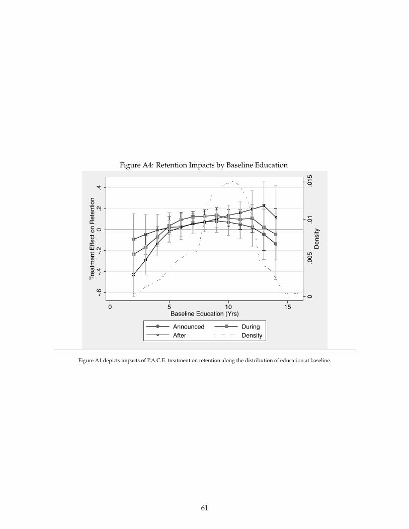
Figure A4: Retention Impacts by Baseline Education

0.0

05.0

1.0

15D

ensi

ty

-.6-.4

-.20

.2.4

Trea

tmen

t Effe

ct o

n R

eten

tion

0 5 10 15Baseline Education (Yrs)


Figure A1 depicts impacts of P.A.C.E. treatment on retention along the distribution of education at baseline.

61

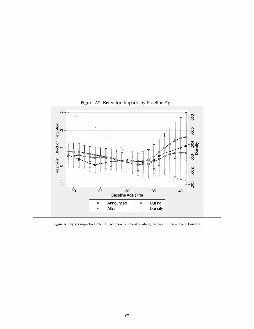
Figure A5: Retention Impacts by Baseline Age

.001

.002

.003

.004

.005

.006

Den

sity

-.10

.1.2

.3Tr

eatm

ent E

ffect

on

Ret

entio

n

20 25 30 35 40Baseline Age (Yrs)


Figure A1 depicts impacts of P.A.C.E. treatment on retention along the distribution of age at baseline.

62

B Data Appendix

B.1 Retention

• 1(Worker Still on Attendance Roster): This variable is defined for each worker i for day d of month

m and year y. It is an indicator variable that is 1 if the worker i is either present in the attendance

data on day d of month m and year y, or is present at a future date, and 0 if the worker stopped

being observed in the attendance data beginning day d of monthm and year y, or any date before.

• 1(Worker Still on Payroll Roster): This variable is defined for each worker i for month m and year

y. An indicator variable that is 1 if the worker i is either present in the payroll data of month

m and year y, or is present at a future date, and 0 if the worker stopped being observed in the

payroll data beginning month m and year y, or any date before.

B.2 Presence, Unauthorized Absence and Tardiness

• Presence: An indicator variable that is 1 if the worker i is present at work on day d of month m

and year y, and 0 otherwise. It is missing if the worker has left the factory i.e. it is conditional on

retention.

• Unauthorized Absence: An indicator variable that is 1 if the worker i is absent at work, and the

absence is not authorized on day d of month m and year y, and 0 if either the worker is present

at work or has taken authorized leave. It is missing if the worker has left the factory i.e. it is

conditional on retention.

• Tardy: An indicator variable that is 1 if the worker i came to the factory later than the modal

worker on their production line, and 0 if they came on time. It is missing if the worker has left

the factory or is not present at work that day.

B.3 Working and Cumulative Man Days

• Working: An indicator variable that is 1 if the worker is retained and present in the factory on day

d of month m and year y, and 0 otherwise (if the worker has left the factory, or is not present that

day). It is thus a combination of retention and attendance, and is not conditional on retention i.e.

it is not missing for workers who have left the factory.

63

• Cumulative Man Days: This measures cumulative man days that accrue to the factory from a par-

ticular worker, as measured by the cumulative sum of the variable Working. As with Working, it

is not conditional on retention.

B.4 Productivity and other Production Variables

• Pieces Produced: Number of garments produced at the hourly level (per worker or per line de-

pending on the regression specification). Line-level number of garments in a given hour is the

average of the number of garments produced at the worker-level.

• Standard Allowable Minutes (SAM): This is a measure of how many minutes a particular garment

style should be completed in. For instance, a garment style with a SAM of .5 is deemed to take

a half minute to produce one complete garment. It is a standardized measure across the global

garment industry and is drawn from an industrial engineering database, although it might be

amended to account for stylistic variations from the representative garment style in the database.

• Target Quantity: The target quantity for a given unit of time for a line producing a particular style

is calculated as the unit of time in minutes divided by the SAM. That is, the target quantity to be

produced by a line in an hour for a style with a SAM of .5 will be60

0.5= 120 garments per hour.

• Efficiency:(

Number of garments producedNumber of target garments

)*100 at the hourly level (per worker or per line de-

pending on the regression specification). Line-level number efficiency in a given hour is the mean

of worker-level efficiency in that hour.

B.5 Career Advancement

B.5.1 Firm’s Administrative Data

This variable varies at the monthly level for each worker.

• Log(Gross Salary): It denotes the natural log of all salaried components of wages (excluding pro-

duction bonuses which are earned at the line level and paid out through a separate system). It is

computed from the firm’s payroll data.

64

B.5.2 Worker Survey Data

These are self-reported measures by the worker during the worker survey implemented after treat-

ment. They vary cross-sectionally at the worker-level.

• Expect Promotion Next 6 Months: An indicator variable that is 1 if the worker reported that they

expect to be promoted in the next 6 months, and 0 otherwise.

• Skill Development Training: An indicator variable that is 1 if the worker reported that they re-

quested skill development training some time in the previous 6 months, and 0 otherwise.

• Production Award Or Incentive: An indicator variable that is 1 if the worker reports that they

received a production incentive bonus any time in the previous 6 months, and 0 otherwise.

• Peer Self-Assessment: Workers were requested to imagine a 6-step ladder on which workers on

their production line that were the same skill-level as them stood according to their ability, where

the worst workers were on the first rung, and the best on the 6th rung. Workers were then asked

which rung they believed they should be on.

• Line Co-Worker Self-Assessment: Workers were requested to imagine a 6-step ladder on which all

the workers on their production line stood according to their ability, where the worst workers

were on the first rung, and the best on the 6th rung. Workers were then asked which rung they

believed they should be on.

B.6 Other Survey Variables

Like the other variables that were collected during the worker survey implemented after treatment,

these variables are self-reported (by the worker), and vary cross-sectionally at the worker-level.

B.6.1 Financial Behaviors and Attitudes

• 1(Any Saving): An indicator variable that takes the value 1 if the worker reports having any

savings, and 0 otherwise.

• Saving for Children’s Education:An indicator variable that takes the value 1 if the worker reports

having saved any money for children’s education, and 0 otherwise.

65

• Risk Aversion Index: Risk aversion was measured from a set of proposed choices between a de-

terministic amount and a gamble. The questions content is the same as those in the Indonesian

Family Life Survey (IFLS), with the amounts under consideration changed to reflect the local

context and currency. For instance, a representative question was:

“Suppose you are given two options of receiving income. In the first option you are guaranteed

Rs. X per month. In the second option you are guaranteed Rs. Y or Rs. Z, each with equal chance.

Which option would you choose?”

The coefficient of risk-aversion assuming CRRA preferences was then computed using the pay-

offs, and solving for the constant of coefficient of risk-aversion. For a detailed description of an

identical computation using the IFLS data, readers are referred to Ng (2013).

B.6.2 Government and Firm Entitlements

• 1(Government Pension): An indicator variable that takes the value 1 if the worker reports having

availed of a government pension program in the last 6 months, and 0 otherwise.

• Government Subsidized Housing: An indicator variable that takes the value 1 if the worker reports

having availed of a government pension program in the last 6 months, and 0 otherwise.

• Firm Subsidized Housing: An indicator variable that takes the value 1 if the worker reports intend-

ing to avail of the employer’s subsidized housing program in the next 6 months, and 0 otherwise.

• Firm Subsidized Schooling: An indicator variable that takes the value 1 if the worker reports in-

tending to avail of the employer’s subsidized schooling program in the next 6 months, and 0

otherwise.

B.6.3 Personality

• Contentiousness (ME): This measure captures the net number of behaviors workers identify with

that are predictive of contentiousness. Workers were asked about the extent (measured on a

5-point scale of agreement ranging from Strongly Agree to Strongly Disagree) to which they

engaged in 5 positive and 5 negative behaviors. The score from each variable was added up for

positive and negative behaviors and the score from the negative behaviors was then subtracted

from the score for positive behaviors.

66

The positive behaviors were the following:

– I am always prepared

– I pay attention to details

– I get chores done right away

– I carry out my plans

– I make plans and stick to them

The negative behaviors were the following:

– I procrastinate and waste my time

– I find it difficult to get down to work

– I do just enough work to get by

– I don’t see things through

– I shirk my duties

The final measure was computed as the mean effect normalization of the above variables.

• Locus of Control (ME): This measure captures the net number of beliefs workers identify with

that are predictive of locus of control. Workers were asked about the extent (measured on a

5-point scale of agreement ranging from Strongly Agree to Strongly Disagree) to which they

believed 5 statements, one of which are positively related to locus of control and four of which are

negatively related. The score from each variable was added up for the negative statements and

the score from the negative statements was then subtracted from the score for positive statement.

The positive statement was the following:

– I believe that my success depends on ability rather than luck

The negative statements were the following:

– I believe that unfortunate events occur because of bad luck

– I believe that the world is controlled by a few powerful people

– I believe some people are born lucky

– I believe in the power of fate

67


• Perseverance (ME): This measure captures the net number of behaviors workers engage in that are

predictive of perseverance. Workers were asked about the extent (measured on a 5-point scale

of agreement ranging from Strongly Agree to Strongly Disagree) to which they engaged in 8

behaviors, five of which are positively related to perseverance and three of which are negatively

related. The score from each variable was added up for the negative statements and the score

from the negative behaviors was then subtracted from the score for positive behaviors.

The positive behaviors were the following:

– I don’t quit a task before it is finished

– I am a goal-oriented person

– I finish things despite obstacles in the way

– I am a hard worker

– I don’t get sidetracked when I work

The negative behaviors were the following:

– I don’t finish what I start

– I give up easily

– I do not tend to stick with what I decide to do


• Extraversion (ME): This measure captures the net number of beliefs workers identify with that

are predictive of extraversion. Workers were asked about the extent (measured on a 5-point

scale of agreement ranging from Strongly Agree to Strongly Disagree) to which they believed 10

statements, five of which are positively related to extraversion and five of which are negatively


from the negative statements was then subtracted from the score for positive statements.

The positive statements were the following:

– Am open about my feelings

68

– Take charge

– Talk to a lot of different people at parties

– Make friends easily

– Never at a loss for words


– Don’t talk a lot

– Keep in the background

– Speak softly

– Have difficulty expressing my feelings

– Hold back my opinions


• Self-Sufficiency (ME): This measure captures the net number of beliefs workers identify with that

are predictive of self-sufficiency. Workers were asked about the extent (measured on a 5-point

scale of agreement ranging from Strongly Agree to Strongly Disagree) to which they believed 10

statements, five of which are positively related to self-sufficiency and five of which are negatively


from the negative statements was then subtracted from the score for positive statements.


– Act without consulting others

– Do things men traditionally do

– Do things my own way

– Make decisions quickly.

– Believe that events in my life are determined only by me


– Need protection

– Often need help.

69

– Talk about my worries.

– Let myself be directed by others.

– Am easily moved to tears.


B.6.4 Mental Health

• Self-Esteem (ME): This measure captures the net number of beliefs workers identify with that are

predictive of self-esteem. Workers were asked about the extent (measured on a 5-point scale of

agreement ranging from Strongly Agree to Strongly Disagree) to which they believed 10 state-

ments, five of which are positively related to self-esteem and four of which are negatively related.

The score from each variable was added up for the negative statements and the score from the

negative statements was then subtracted from the score for positive statements.


– On the whole, I am satisfied with myself

– I feel that I have a number of good qualities

– I am able to do things as well as most other people

– I feel that I am person of worth, at least on an equal plane with others

– I take a positive attitude toward myself


– I feel I do not have much to be proud of

– At times, I think I am no good at all

– I certainly feel useless at times

– I wish I could have more respect for myself

– All in all, I am inclined to feel that I am a failure


• Hope or Optimism (ME): This measure captures the net number of beliefs workers identify with

that are predictive of hope or optimism. Workers were asked about the extent (measured on a

70

5-point scale of agreement ranging from Strongly Agree to Strongly Disagree) to which they be-

lieved 10 statements, five of which are positively related to hope or optimism and three which

are negatively related. The score from each variable was added up for the negative statements

and the score from the negative statements was then subtracted from the score for positive state-

ments.


– Look on the bright side.

– Can find the positive in what seems negative to others.

– Remain hopeful despite challenges.

– Will succeed with the goals I set for myself.

– Think about what is good in my life when I feel down.


– Expect the worst.

– Have no plan for my life five years from now.

– Am not confident that my way of doing things will work out for the best


• Mental Distress: The two measures of mental health are computed using the 10-question Kessler

Psychological Distress Scale, or K10. The K10 was developed by Ron Kessler and Dan Mroczek

in 1992 as a measure of mental distress (Kessler et al., 2003). The questionnaire consists of 10

questions about negative emotional states experienced during the past 4 weeks. Respondents

give 5-point answers ranging from “none of the time” (scored as a 1) to “all of the time” (scored

as a 5), with the intermediate responses scored correspondingly (i.e. “a little of the time” scored as

2, “some of the time” scored as 3, and “most of the time” scored as 4). In particular, respondents

are asked:

– About how often did you feel tired out for no good reason?

– About how often did you feel nervous?

– About how often did you feel so nervous that nothing could calm you down?

71

– About how often did you feel hopeless?

– About how often did you feel restless or fidgety?

– About how often did you feel so restless you could not sit still?

– About how often did you feel depressed?

– About how often did you feel that everything was an effort?

– About how often did you feel so sad that nothing could cheer you up?

– About how often did you feel worthless?

The survey methodology was developed and first validated in the United States. It has since been

administered in a variety of contexts around the world, including in low-income populations in

South Africa (Myer et al., 2008). Moderate mental distress is indicated by a score of 24 or higher

on the scale.

72

the skills to pay the bills: returns to on-the-job soft

Documents