the skills to pay the bills: returns to on-the-job soft skills ... skills to pay the bills: returns...

NBER WORKING PAPER SERIES

THE SKILLS TO PAY THE BILLS:RETURNS TO ON-THE-JOB SOFT SKILLS TRAINING

Achyuta AdhvaryuNamrata Kala

Anant Nyshadham

Working Paper 24313http://www.nber.org/papers/w24313

NATIONAL BUREAU OF ECONOMIC RESEARCH1050 Massachusetts Avenue

Cambridge, MA 02138February 2018

We are very grateful to Anant Ahuja, Chitra Ramdas, Raghuram Nayaka, Sudhakar Bheemarao, and Paul Ouseph for their coordination, enthusiasm, and guidance. Thanks to Dotti Hatcher, Lucien Chan, Noel Simpkin, and others at Gap, Inc. for their support and feedback on this work. We acknowledge funding from Private Enterprise Development in Low-Income Countries (PEDL) initiative, and Adhvaryu’s NIH/NICHD (5K01HD071949) career development award. This research has benefited from discussions with Michael Boozer, Robert Gibbons, Paul Gertler, Markus Goldstein, Rocco Macchiavello, David McKenzie, Dilip Mookherjee, Claudia Olivetti, Antoinette Schoar, Tavneet Suri, Chris Udry, John Van Reenen, and Chris Woodruff, and seminar audiences at NBER, Penn, MIT, USC, Madrid, PEDL, IGC, World Bank, AEA, Northeastern, NEUDC, Chicago, Michigan, McGill, Georgetown, and Copenhagen. Many thanks to Lavanya Garg, Robert Fletcher, and Aakash Mohpal for excellent research assistance. The views expressed herein do not represent PEDL, NIH, Gap, Inc., or Shahi Exports. All errors are our own. The views expressed herein are those of the authors and do not necessarily reflect the views of the National Bureau of Economic Research.

NBER working papers are circulated for discussion and comment purposes. They have not been peer-reviewed or been subject to the review by the NBER Board of Directors that accompanies official NBER publications.

© 2018 by Achyuta Adhvaryu, Namrata Kala, and Anant Nyshadham. All rights reserved. Short sections of text, not to exceed two paragraphs, may be quoted without explicit permission provided that full credit, including © notice, is given to the source.

The Skills to Pay the Bills: Returns to On-the-job Soft Skills TrainingAchyuta Adhvaryu, Namrata Kala, and Anant NyshadhamNBER Working Paper No. 24313February 2018JEL No. J24,M53,O15

ABSTRACT

We evaluate the causal impacts of on-the-job soft skills training on the productivity, wages, and retention of female garment workers in India. The program increased women’s extraversion and communication, and spurred technical skill upgrading. Treated workers were 20 percent more productive than controls post-program. Wages rise very modestly with treatment (by 0.5 percent), with no differential turnover, suggesting that although soft skills raise workers’ marginal products, labor market frictions are large enough to create a substantial wedge between productivity and wages. Consistent with this, the net return to the firm was large: 258 percent eight months after program completion.

Achyuta AdhvaryuRoss School of BusinessUniversity of Michigan701 Tappan StreetAnn Arbor, MI 48109and [email protected]

Namrata KalaHarvard University27 Hillhouse AveNew Haven, CT [email protected]

Anant NyshadhamDepartment of EconomicsBoston CollegeMaloney Hall, 324Chestnut Hill, MA 02467and [email protected]

An online appendix is available at http://www.nber.org/data-appendix/w24313

1 Introduction

Soft skills – e.g., teamwork, leadership, relationship management, personality factors, effective timeallocation, and the ability to assimilate information – are highly predictive of success in the labormarket (Bassi et al., 2017; Borghans et al., 2008; Deming, 2015; Groh et al., 2015; Guerra et al., 2014;Heckman and Kautz, 2012; Heckman et al., 2006; Montalvao et al., 2017). Surveys of employers fromaround the world corroborate that soft skills are in great demand, and that firms often struggle to findworkers with high levels of these skills (Cunningham and Villasenor, 2016).

Studies from psychology and economics demonstrate that it is possible to inculcate soft skills inearly childhood, via, for example, home-based stimulation and high quality preschool programs (At-tanasio et al., 2014; Gertler et al., 2014; Grantham-McGregor et al., 1991; Ibarraran et al., 2015). But howmalleable soft skills are in adulthood, and whether training programs that aim to increase the stockof these skills can indeed generate causal impacts on productivity, have only begun to be explored(Acevedo et al., 2017; Ashraf et al., 2017; Campos et al., 2017; Groh et al., 2012). It is not obvious thatinculcating these skills in a meaningful way is possible: structural estimates of dynamic human capitalaccumulation models suggest that it may indeed be difficult to affect non-cognitive skill levels at laterages, particularly for those with low baseline stocks, due to dynamic complementarities (Aizer andCunha, 2012; Cunha et al., 2010; Heckman and Mosso, 2014).

Moreover, when general training is delivered within the firm (as it often is1), it is imperative toknow the firm’s returns to training in addition to worker productivity effects. This impact, in turn, isgoverned by labor market structure. In perfectly competitive markets, workers’ wages would need toincrease commensurate to their marginal products; any firm that paid below marginal product wouldlose the newly trained workers as they received higher wage offers at other firms. As Becker (1964)famously noted, this implies that with perfect labor markets, even general training programs thatgenerate large productivity returns may not be appealing investments for firms. On the other hand, ifasymmetric information and search frictions play a role in the labor market, then the resulting wedgebetween workers’ marginal products and their wages in equilibrium may create positive productivityrents from general training for firms (Acemoglu, 1997; Acemoglu and Pischke, 1998, 1999; Autor, 2001;Chang and Wang, 1996; Katz and Ziderman, 1990). Since most soft skills are “general,” the extent oflabor market frictions thus likely polices the ability to deliver soft skills training through firms, evenwhen training raises productivity.

The questions that motivate our study, then, are threefold. First, is it possible to improve soft skillsmeaningfully for workers with low stocks of these skills? Second, if skills do improve, what are thecausal impacts on workplace outcomes, including productivity, wages, and retention? Finally does itpay for firms to provide on-the-job soft skills training to workers, and what does this rate of return tellus about the nature of labor market frictions as pertains to soft skills?

To answer these questions, we partnered with the largest ready-made garment export firm in Indiato evaluate an intensive, workplace-based soft skills training program. The initiative, which is namedPersonal Advancement and Career Enhancement (P.A.C.E.), aims to empower female garment workersvia training in a broad variety of life skills, including modules on communication, time management,

1See, e.g., Bassanini et al. (2007).

2

financial literacy, successful task execution, and problem-solving. These skills are important inputsinto production in the ready-made garments context. Workers need effective communication to resolvethroughput issues with other team members (e.g., identifying and working through bottlenecks inreal time). They need relationship management skills to relay information in a productive way tosupervisors (e.g., machine malfunction, requesting breaks or help to complete tasks, etc.). And theyneed problem-solving frameworks to effectively deal with daily shocks to production.

We conducted a randomized controlled trial (RCT) in five garment factories in urban Bengaluru,India. We assessed the impacts of soft skills training on 1) direct and indirect measures of the stock ofthese skills; and 2) administrative data on retention, productivity, wages, task complexity, and otherworkplace outcomes. Finally, we compute the firm’s returns, combining our point estimates with dataon the program’s costs and the firm’s accounting profits.

We enrolled female garment workers in a lottery for the chance to take part in the P.A.C.E. programand used a two-stage randomization procedure to assign workers to treatment. In the first stage, werandomized production lines to treatment. In the second stage, within treatment lines, we randomizedworkers who had enrolled in the lottery to either direct P.A.C.E. training or spillover treatment. Wethus estimate treatment effects by comparing trained workers (on treatment lines) to control workerson control lines (who enrolled in the lottery but whose lines were assigned to control). We estimatespillovers by comparing untrained workers on treatment lines to control workers on control lines.

Endline survey results for treated and control workers and pre/post-module testing of treatedworkers indicate that stocks of soft skills improved in several important dimensions. Specifically,treated women showed a pronounced increase in extraversion, which may impact productivity viaimprovements in the ability to communicate and solve issues collaboratively with peers and supervi-sors. These women were also more likely to request and complete technical skill development train-ings, generating complementary improvements in “hard” skills. Survey results indicate greater self-assessment of workplace quality (relative to peers of the same technical skill grade), consistent with anincrease in self-regard. Finally, pre/post data from assessment tools designed to measure learning ineach of the program’s modules show that initial stocks of knowledge in each of the program’s targetareas were low, and that treated workers substantially improved these stocks through the program(most markedly for communication skills).

Direct impacts on workplace outcomes, measured using the firm’s administrative data, are con-sistent with the acquisition of soft skills by workers. Treated workers are more productive by about11 percentage points (20% higher than the control mean) and more likely to be assigned to complextasks. Impacts last up to 8 months after program completion (when we ceased data collection), sug-gesting that learned skills translated into persistent improvements in workplace outcomes. Workerson treatment lines who did not receive the program are also more productive and are assigned to morecomplex operations, generating team-level (production line) impacts on productivity post-programcompletion. Wages went up very slightly as a result of treatment: an increase of about 0.5 percent. Theprogram had no sustained impact on turnover. Retention was actually higher in the treatment grouprelative to control during the program period; this effect diminished after program completion.2

2We use a dynamic inverse probability weighting procedure, described in detail in section 4, throughout our analysis tocorrect for potential changes in the size and composition of the treatment and control groups over time.

3

Taken in sum, we interpret the results to indicate that the program increased workers’ stocks ofsoft skills, which in turn led to productivity improvements.3 Combined with the fact that there wasessentially no impact on wage or long-run turnover, our results suggest the presence of substantiallabor market frictions that prevent workers from capturing more of the productivity rents that ensuefrom training (Acemoglu, 1997; Acemoglu and Pischke, 1999). The nature of the hiring process in thislabor market helps to rationalize this result. Specifically, sewing machine operators are evaluated – andaccordingly are given wage offers – based only on stitching skills. Soft skills are largely unobservedin this hiring process and therefore are not priced into the wage, in line with other hiring processesfor frontline workers in low-income country contexts (Bassi et al., 2017). This information frictionlikely generates the observed difference in impacts of soft skills training on marginal productivity ascompared to wage.

We use our estimates of impacts on workplace outcomes along with program cost and accountingprofit data to calculate the costs and benefits of the program to the firm. The net rate of return was 73%by the end of the program period. Eight months after program completion, fueled by post-programincreases in productivity, the return climbed to over 250%. These large returns are rationalized by therelatively low costs of the program combined with the accumulated effects on productivity and persondays, and are consistent with other recent interventions in garment factories in South Asia (Menzel,2015).

Our main contribution is to the study of soft skills in the labor market. We join a handful of recentstudies that evaluate the causal impacts of soft skills training on economic outcomes (Acevedo et al.,2017; Ashraf et al., 2017; Campos et al., 2017; Groh et al., 2012; Schoar, 2014). We add to this workby studying training within the firm, which emphasizes estimating firms’ returns, tying our work tothe literature on the role of labor market frictions in firms’ decisions to train their workers (Acemoglu,1997; Acemoglu and Pischke, 1998, 1999; Autor, 2001). We are also able to directly estimate impacts onindividual productivity, which is missing from previous work.4

Other previous work quantifying the productivity impacts of on-the-job training generally uses ob-servational data on firms and workers in the United States and Western Europe (Barrett and O’Connell,2001; Barron et al., 1999; Dearden et al., 2006; Konings and Vanormelingen, 2015; Mincer, 1962). Thesestudies tend to find that training increases productivity, but there is disagreement on the magnitudeof this increase (Blundell et al., 1999). Specifically, when endogeneity of training is accounted for (e.g.,using matching methods), productivity returns become quite small (Goux and Maurin, 2000; Leuvenand Oosterbeek, 2008). We add to this literature in three ways. First, we estimate causal effects byexploiting randomized assignment to training, which overcomes potential self-selection bias (Altonjiand Spletzer, 1991; Bartel and Sicherman, 1998). Second, we estimate impacts on retention in additionto productivity; retention is crucial to understanding firms’ overall returns to training but has not beenexamined thus far. Third, we carry out our experiment in a low-income country setting, where trainingfrontline workers might have large potential given low levels of baseline skills.

The rest of the paper is organized as follows. Section 2 discusses the garment production context

3We address several other possible mechanisms in section 6, including potential changes to mental and physical health,reciprocity, and social capital.

4Campos et al. (2017) measure microenterprise profits, which of course are in part a function of productivity.

4

and reviews the details of the training program and the experimental design. Section 3 discussesthe data sources and the construction of key variables, and section 4 describes the estimation strategy.Section 5 describes the results of the estimation. Section 6 discusses and evaluates possible mechanismsand presents an analysis of the costs and benefits to the firm. Section 7 concludes.

2 Context, Program Details, and Experiment Design

2.1 Context

2.1.1 Ready-made Garments in India

Apparel is one of the largest export sectors in the world, and vitally important for the economies ofseveral large developing countries (Staritz, 2010). India is one of the world’s largest producers of textileand garments, with export value totaling $10.7 billion in 2009-2010. The size of the sector and the labor-intensity of the garment production process make the sector well-suited to absorb the influx of young,unskilled and semi-skilled labor migrating from rural self-employment to wage labor in urban areas,especially women (World Bank, 2012). Women comprise the majority of the workforce in garmentfactories, and new labor force entrants tend to be disproportionately female, particularly in countrieslike India where the baseline female labor force participation rate is low (Staritz, 2010). Shahi Exports,Private Limited, the firm with which we partnered to do this study, is the largest private garmentexporter in India, and the single largest private employer of unskilled and semi-skilled female labor inthe country.

2.1.2 The Garment Production Process

There are three broad stages of garment production: cutting, sewing, and finishing. In this study, weestimate program impacts on workers from the sewing department only, as measures of individualproductivity and task complexity are only available for sewing workers.5 Sewing department workersmake up about 80% of the factory’s total employment.

In the sewing department of the study factories (as in most medium and large garment factories),garments are sewn in production lines consisting of around 50-70 workers arranged in sequence. Mostof the workers on the line are assigned to machines completing sewing tasks (one person to a ma-chine). The remaining workers perform complementary tasks to sewing, such as folding or aligningthe garment to feed it into a machine. Each line produces a single style of garment at a time.6

The line is subdivided into smaller groups of operations that produce subsections of the garment(e.g., collar, sleeve, or pocket). These groups are separated by “feeding points” at which the preparedmaterials for each subsection of the garment are fed in bundles (e.g., materials for 20 pockets or collarsof the current shirt will be fed at one point and materials for 40 sleeves will be fed at the next point).This structure of subdivisions, multiple feeding points, and bundles of materials is very common in

5This is because a standardized measure of output is recorded for each worker in each hour on the sewing floor, but sucha measure is not recorded for workers in other departments.

6The color and size of the garment might vary but the design and style will be the same for every garment produced bythat line until the ordered quantity for that garment is met.

5

the industry (and in fact mirrored in many other manufacturing industries) and is used explicitly todecouple, as much as is possible, productivity at adjacent operations or subdivisions and allow timefor rebalancing of productivity across the line.

Completed sections of garments pass between machine operators in these bundles, are attachedto each other in additional operations along the way, and emerge at the end of the line as completedgarments. These completed garments are then transferred to the finishing floor. In the finishing de-partment, garments are checked, ironed, and packed for shipping. Most quality checking is done onthe sewing floor during production, but final checks are done in the finishing stage. Any garmentswith quality issues are sent back to the sewing floor for rework or, if irreparably ruined, are discardedbefore packing.7 Orders are then packed and sent to ports for export.

2.2 Program Details

The Personal Advancement and Career Enhancement (P.A.C.E.) program was designed and first im-plemented by Gap, Inc. for female garment workers in low-income contexts. Shahi Exports partici-pated in the original design and piloting of the program as one of the largest suppliers to Gap. Theintervention we study involved the implementation of the P.A.C.E. program in five factories in theBengaluru area which had not yet adopted the program. The goal of this 80-hour program was toimprove life skills such as time management, effective communication, problem-solving, and financialliteracy for its trainees. The program began with an introductory ceremony for participants, trainers,and firm management. The core modules were: Communication (9.5 hours); Problem Solving andDecision-Making (13 hours); Time and Stress Management (12 hours); Execution Excellence (5 hours);Financial Literacy (4.5 hours); and Legal Literacy and Social Entitlements (8.5 hours).8 Table A1 pro-vides an overview of the topics covered in each module. After all modules had been completed, therewere two review sessions (3 hours in total) reiterating concepts from early modules and discussinghow participants would apply their learning to personal and professional situations. At the close ofthe program there was a graduation ceremony.

Workers participated in two hours of training per week. Management allocated one hour of work-ers’ production time a week to the program, and workers contributed one hour of their own time.Training sessions were conducted at the beginning of the production day in designated classroomspaces in the factories, with workers assigned to groups corresponding to different days of the workweek. That is, a worker assigned to the Monday group would be expected to attend training startingone hour before production starts on each Monday and ending after the first production hour of theday is completed (two hours in total). Production constraints required that each day’s group be com-posed of workers from across production lines so as not to produce large, unbalanced absences fromany one line in the first hour of any production day. Accordingly, the training groups were balancedin size with roughly 50 trainees per class and no more than 3-4 from a given line in each group.

7Completed quantities of garments recorded in the production data reflect only pieces which have passed quality checks,so quantity produced reflects both quantity and minimum quality combined.

8Additional modules on Water, Sanitation and Hygiene (6 hours) and General and Reproductive Health (10 hours) werealso included, but were not considered core modules. Pre/post assessments were not conducted for ancillary modules suchas sanitation.

6

Due to holidays and festivals (which are times of high absenteeism), sessions were conducted inpractice somewhat more flexibly with respect to timing. Catch-up sessions were conducted for workerswho were unable to attend a session. This flexibility is reflected in average attendance (of non-attritedworkers) to the core program modules, which was very high, ranging between 94 and 99 percent (seeFigure A12). With these adjustments, overall program implementation took about 12 months: theintroductory ceremony was in July 2013, training was conducted between July 2013 and June 2014,and the closing ceremony in July 2014.

Figure 1A: Experimental Design

5 factories; 112production lines;

2703 workers(signed up for aP.A.C.E. lottery)

Treatment= 80 lines

Control= 32 lines

Treated=1087 workers

Spillover (ontreatment

line, but notenrolled)=

837 workers

Control (oncontrol lines)=779 workers

Figure 1B: Timeline of Experiment and Data Collection

January 2013 • Salary and Attendance Data Collection StartsJune 2013 • Treatment Assignment Announcement and Productivity Data Collection StartsJuly 2013 • Training Program Starts (Pre and Post Module Testing During Training)June 2014 • Training Program Ends and Worker Survey Conducted

December 2014 • Salary Data Collection EndsFebruary 2015 • Attendance and Production Data Collection Ends

2.3 Experimental Design

Participants were chosen from a pool of workers who expressed interest and committed to enroll inthe program. The workers were informed that the training was oversubscribed and that a subset ofworkers would be chosen at random from a lottery to actually receive the training, with untreated

7

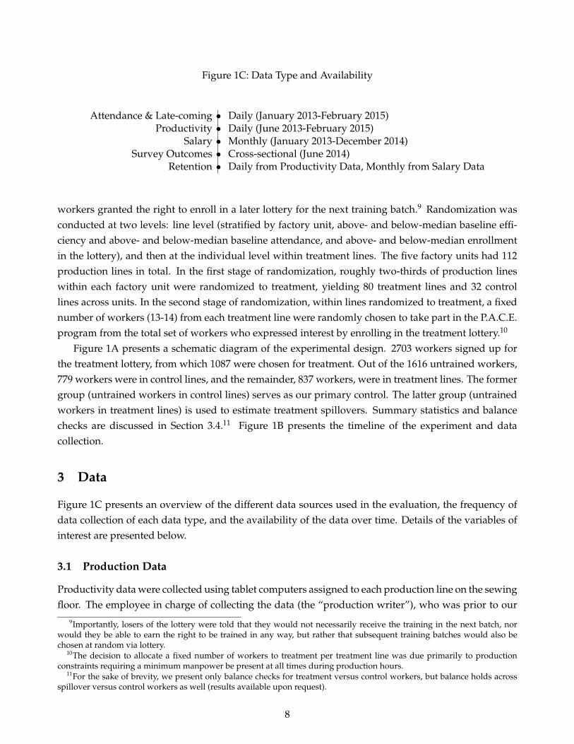
Figure 1C: Data Type and Availability

Attendance & Late-coming • Daily (January 2013-February 2015)Productivity • Daily (June 2013-February 2015)

Salary • Monthly (January 2013-December 2014)Survey Outcomes • Cross-sectional (June 2014)

Retention • Daily from Productivity Data, Monthly from Salary Data

workers granted the right to enroll in a later lottery for the next training batch.9 Randomization wasconducted at two levels: line level (stratified by factory unit, above- and below-median baseline effi-ciency and above- and below-median baseline attendance, and above- and below-median enrollmentin the lottery), and then at the individual level within treatment lines. The five factory units had 112production lines in total. In the first stage of randomization, roughly two-thirds of production lineswithin each factory unit were randomized to treatment, yielding 80 treatment lines and 32 controllines across units. In the second stage of randomization, within lines randomized to treatment, a fixednumber of workers (13-14) from each treatment line were randomly chosen to take part in the P.A.C.E.program from the total set of workers who expressed interest by enrolling in the treatment lottery.10

Figure 1A presents a schematic diagram of the experimental design. 2703 workers signed up forthe treatment lottery, from which 1087 were chosen for treatment. Out of the 1616 untrained workers,779 workers were in control lines, and the remainder, 837 workers, were in treatment lines. The formergroup (untrained workers in control lines) serves as our primary control. The latter group (untrainedworkers in treatment lines) is used to estimate treatment spillovers. Summary statistics and balancechecks are discussed in Section 3.4.11 Figure 1B presents the timeline of the experiment and datacollection.

3 Data

Figure 1C presents an overview of the different data sources used in the evaluation, the frequency ofdata collection of each data type, and the availability of the data over time. Details of the variables ofinterest are presented below.

3.1 Production Data

Productivity data were collected using tablet computers assigned to each production line on the sewingfloor. The employee in charge of collecting the data (the “production writer”), who was prior to our

9Importantly, losers of the lottery were told that they would not necessarily receive the training in the next batch, norwould they be able to earn the right to be trained in any way, but rather that subsequent training batches would also bechosen at random via lottery.

10The decision to allocate a fixed number of workers to treatment per treatment line was due primarily to productionconstraints requiring a minimum manpower be present at all times during production hours.

11For the sake of brevity, we present only balance checks for treatment versus control workers, but balance holds acrossspillover versus control workers as well (results available upon request).

8

intervention charged with recording by hand on paper each machine operator’s completed operationseach hour for the line, was trained to input production data directly in the tablet computer instead.These data then automatically wirelessly synced to the server. Importantly, from the perspective of thegarment workers, production data were being recorded identically before, during, and after the inter-vention across treatment and control lines. Note that though productivity was being recorded priorto the program implementation, the worker-hourly level data was not kept prior to the introductionof the tablet computers for production writing but rather discarded after line-daily level aggregatemeasures were input into the data server. Accordingly, line-daily level aggregate data was all that wasavailable at the time of treatment assignment, and as mentioned above, the first stage randomizationof lines to treatment was stratified by line-level baseline efficiency.

3.1.1 Productivity

The key measure of productivity we study is efficiency. Efficiency is calculated as pieces produceddivided by the target quantity of pieces per unit time. In order to calculate the worker-level dailymean of production from these observations, we average the efficiency of each worker over the courseof the day (8 production hours).12

At the worker-hour level, we define pieces produced as the number of garments that passed aworker’s station by the end of that production hour. For example, if a worker was assigned to sewplackets onto shirt fronts, the number of shirt fronts at that worker’s station that had completedplacket attachment by the end of a given production hour would be recorded as that worker’s “piecesproduced.” The target quantity for a given operation is calculated using a measure of garment andoperation complexity called the “standard allowable minute” (SAM). SAM is defined as the number ofminutes required for a single garment of a particular style to be produced. That is, a garment style witha SAM of 30 is deemed to take half an hour to produce one complete garment. This measure at the linelevel is then decomposed into worker or task specific increments. A line with 60 machine operatorsthen would have an average worker-hourly SAM of 0.5.13 As the name suggests, it is standardizedacross the global garment industry and is drawn from an industrial engineering database.14 The targetquantity for a given unit of time for a worker completing a particular operation is then calculated asthe unit of time in minutes divided by the SAM. That is, the target quantity of pieces to be producedby a worker in an hour for an operation with a SAM of 0.5 will be 60/.5 = 120.

As mentioned in the previous section, hourly productivity data was available starting the month oftreatment announcement. During the month of treatment announcement (June 2013) the tablets wereintroduced onto the production floors. Accordingly, June 2013 represents the pre-program baseline forall productivity analysis below.

12As noted above, pieces are recorded only if the garment is complete and passes minimum quality standards during in-line and end-line quality checking. In averaging across hourly quantities within the day, we expect that mis-measurementarising from re-worked defective pieces is minimized.

13Mean SAM across worker hourly observations is 0.61 with a standard deviation of 0.20.14This measure may be amended to account for stylistic variations from the representative garment style in the database.

Any amendments are explored and suggested by the sampling department, in which master tailors make samples of eachspecific style to be produced by lines on the sewing floor (for costing purposes).

9

3.2 Human Resources Data: Attendance and Salary

Data on demographic characteristics, attendance, tenure and salary of workers are kept in a firm-managed database. The data linked to worker ID numbers were shared with us. The variables avail-able in demographic data include age, date on which the worker joined the firm, gender, native lan-guage, and education. We combined these with daily attendance data at the worker level indexed byworker ID number and date, which records whether a worker attended work on a given date, whetherabsence was authorized or not, and whether a worker was late to work on a given day (worker tardi-ness). We also combined these with monthly salary data which also indicates current skill grade level.The salary data are available until six months post-program completion, unlike the productivity andattendance data, which are available for eight months after program completion.

3.3 Survey Data

In addition to measuring workplace outcomes, a survey of 1000 randomly chosen treated and controlworkers was conducted in June 2014, the month of program completion. The survey covered, amongother things, questions related to financial decisions (including savings and debt) and awareness of andparticipation in welfare programs (government or employer sponsored). It also measured personalitycharacteristics (conscientiousness, extraversion, locus of control, perseverance, and self-sufficiency),mental health (hope/optimism, self-esteem, and the Kessler 10 module, which can be used to diag-nose moderate to severe psychological distress (Kessler et al., 2003)), and risk and time preferenceselicited using lottery choices.15 Finally, the survey covered worker’s self-assessments relative to peersby asking them to imagine a six-step ladder with the lowest productivity workers on the lowest steps,and then asking them which step they would place themselves on; participation in skill developmentprograms; production awards; and incentive programs on the job.

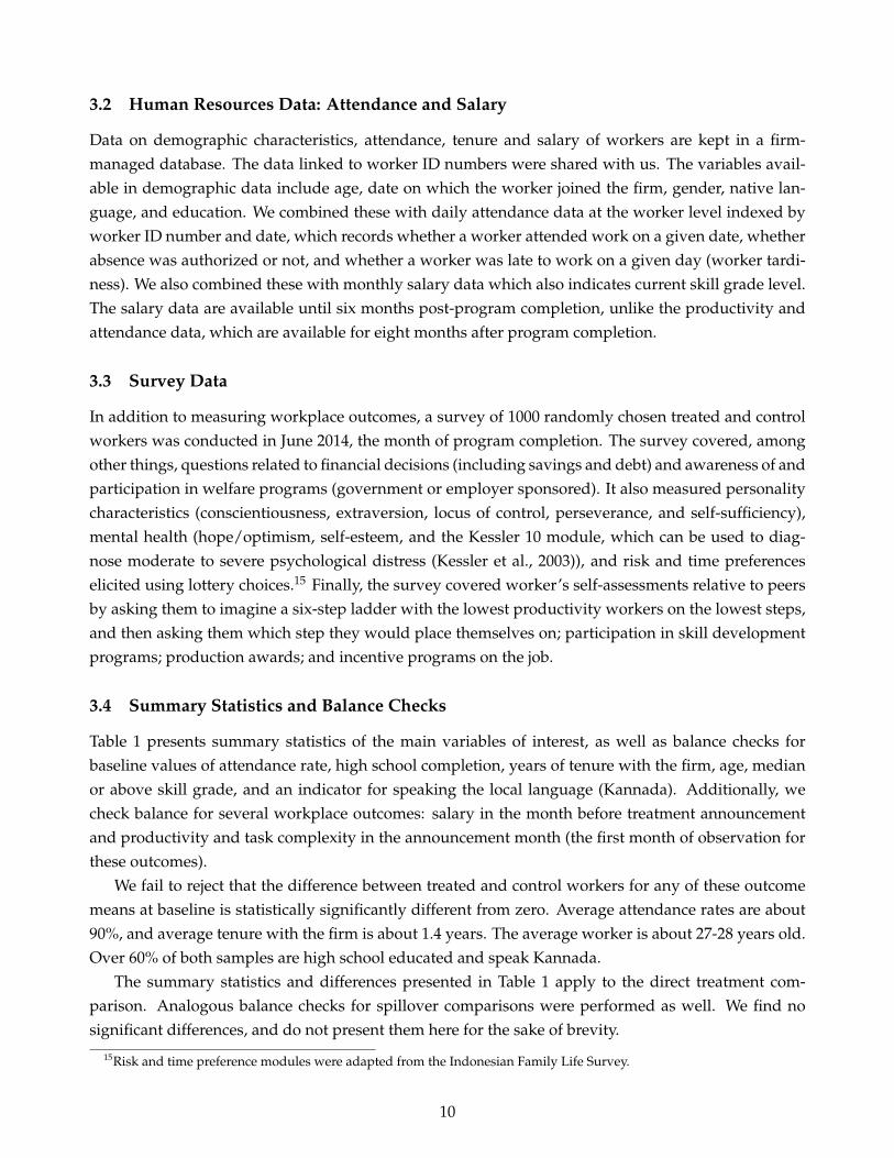
3.4 Summary Statistics and Balance Checks

Table 1 presents summary statistics of the main variables of interest, as well as balance checks forbaseline values of attendance rate, high school completion, years of tenure with the firm, age, medianor above skill grade, and an indicator for speaking the local language (Kannada). Additionally, wecheck balance for several workplace outcomes: salary in the month before treatment announcementand productivity and task complexity in the announcement month (the first month of observation forthese outcomes).

We fail to reject that the difference between treated and control workers for any of these outcomemeans at baseline is statistically significantly different from zero. Average attendance rates are about90%, and average tenure with the firm is about 1.4 years. The average worker is about 27-28 years old.Over 60% of both samples are high school educated and speak Kannada.

The summary statistics and differences presented in Table 1 apply to the direct treatment com-parison. Analogous balance checks for spillover comparisons were performed as well. We find nosignificant differences, and do not present them here for the sake of brevity.

15Risk and time preference modules were adapted from the Indonesian Family Life Survey.

10

Table 1: Summary Statistics

P.A.C.E. Treatment Number of workers

Mean SD Mean SD Mean Difference p value

Attendance Rate (Jan-May 2013) 0.898 0.117 0.903 0.103 -0.005 0.380 High School 0.602 0.489 0.604 0.489 -0.003 0.901 Years of Tenure 1.432 2.709 1.353 2.119 0.079 0.500 Age 27.712 14.087 27.420 11.638 0.292 0.637 1(Speaks Kannada) 0.657 1.560 0.671 1.156 -0.014 0.834 High Skill Grade 0.616 0.843 0.642 0.688 -0.026 0.473 log(Salary) (May 2013) 8.746 0.188 8.737 0.156 0.009 0.258 Efficiency (Announcement Month) 0.586 0.587 0.556 0.426 0.030 0.268 SAM (Announcement Month) 0.618 0.726 0.615 0.535 0.003 0.928

Spillover Treatment Number of workers

(1)Control

(2)Treated

(3)Difference

Control Workers in Control Lines Treated Workers in Treatment Lines779 1,087

Notes: Tests of differences calculated using errors clustered at the line level according to the experimental design.

Control Workers in Control Lines Control Workers in Treatment Lines779 837

4 Empirical Strategy

4.1 Overview

The empirical analysis proceeds in several steps, beginning with testing the impact of the program onretention. This is important as a first step because impacts on retention would necessitate a weightingprocedure to account for the differential attrition across treatment and control groups. Following this,we test for differences in workplace outcomes, then for differences in survey measures of self-reportedpersonal and professional outcomes, and finally estimate treatment spillovers.

4.2 Retention, Working, and Cumulative Person Days

We estimate the following regression specification to test whether P.A.C.E. treatment impacts retention:

Rwdmy = α0 + ζ11[Tw] ∗ 1[Treatment Announced]my + ζ21[Tw] ∗ 1[During Treatment]my+

ζ31[Tw] ∗ 1[After Treatment]my + ψuym + ηw + εwdmy

(1)

where the outcome is an indicator variable that takes the value 1 if worker w was retained on day d inmonthm and year y and 0 otherwise, 1[Tw] is a dummy variable that takes the value 1 if the worker is atrained worker on a treatment line and 0 if she is a control worker on a control line, and it is interactedwith dummies that take the value 1 for the month that the assignment to treatment was announced, themonths during the treatment and the months post-treatment, respectively, thus allowing comparisonrelative to the pre-announcement period. Each regression includes unit x year x month fixed effectsψuym (which absorb the main effects of the time dummies) and worker fixed effects ηw (which absorbthe main effect of the treatment indicator).

11

We estimate equation 1 separately for retention dummy variables constructed using both dailyattendance data and monthly payroll data. The difference between the two is that with the dailydata we can see whether the worker stopped coming to work within the month, even before they areremoved from the payroll. Standard errors are clustered at the production line level - while we did atwo level randomized treatment assignment with the lower level of treatment at the worker level, wereport line level clustering to be as conservative as possible. This is particularly important since wedesigned the experiment to measure spillover effects, and in fact find some evidence to this effect.

To estimate the impact of treatment on the additional number of days the firm receives from theworker, we consider two outcomes: the first is a binary working variable that is 1 if the worker wasretained and is present in the the factory on a given day and 0 otherwise. It is thus a combinationof retention and attendance. The second is the number of cumulative person days as measured bythe cumulative running sum of the first variable. Both are defined at the daily level for each worker.They are estimated as in Equation 1 using these variables instead of retention on the left-hand side.These variables can once again be calculated from two sources of raw data: attendance and productionrosters.

4.3 Dealing with Potential Bias from Selective Attrition

When examining conditionally observed outcomes such as productivity (which are only observed ifthe worker is still at the firm and working that day), there is a potential for selective attrition or obser-vation based on treatment, which could generate bias in the impact estimates. To test and account forthis potential bias, we follow several approaches, outlined below.

1. Testing directly for treatment-induced changes in the relative size of treatment v. control groups: Wetest directly for differential retention by estimating the regression specification in Equation 1shown above. We present the results in Section 5.1. The results indicate there was no differentialretention at the end point of the program period (July 2014) as well as any point afterward.

2. Balance tests by baseline characteristics at different points during and post-program completion: To testwhether the retention across treatment and control is correlated with baseline characteristics, wepresent the results of balance tests by treatment and control one month after treatment (July 2014)as well as during the last month of data collection (February 2015). Results are presented in TableA9; the analysis shown here demonstrates that all baseline characteristics are balanced on meansat both points in time. Tests conducted for other points in time are also balanced and omittedhere for brevity. In addition, there is no heterogeneity in retention impacts across distributionsof baseline characteristics at treatment announcement, program completion, and data collectionendline, as shown in Figures A1-A6 (which provide a more stringent test than balance checksbased on means).

3. Dynamic weighting of conditionally observed outcomes: As mentioned above, we do not find anydifferential retention at the end point of the program period, nor do we find any evidence ofheterogeneity in retention across treatment and control groups for any baseline characteristics.

12

Despite this, in order to confidently recover population average treatment effects on condition-ally observed outcomes throughout the observation period, we weight treatment and controlgroups by the probability of being observed at any intermediate point in the data. For exam-ple, if there exists differential attrition across treatment and control at 6 months into programimplementation, even if this difference later equalizes, to ensure that we recover the populationaverage treatment effect on any conditionally observed outcome (e.g., productivity or salary) atall subsequent points of observation, we can weight all observations prior to that time by theprobability of being able to measure the outcome at each point in time. Accordingly, we adaptthe approach proposed in Wooldridge (2010) to accommodate any potential heterogeneous im-pacts of treatment by baseline characteristics of the workers and any differential dynamics in theonset or decay of treatment effects across time, in the following manner:

(a) Estimate a probit specification for the probability of being observed, which is a dummyvariable that takes the value 1 if the worker is in the sample on any given month and 0 oth-erwise (i.e., the retained dummy if studying impacts from the attendance or salary data andthe working dummy if studying impacts from the production data), on the treatment indi-cator interacted with month by year fixed effects and baseline characteristics (attendance,education, tenure, age, skill grade, productivity and task complexity).16

(b) We then estimate equation 1 using the conditionally observed outcome variables on the left-hand side and the inverse of the predicted probabilities from the first step as probabilityweights. Note that because in the intermediate data (after the announcement but before theendline) the control group is less likely to be working (as shown in the results), this amountsto overweighting a subset of control observations at most points along the timeline.

In practice, once worker fixed effects are included in all regressions, the weighting procedurehas negligible effect on the results. We explored robustness to different weights, as well as theabsence of weights altogether, but do not present these results for the sake of brevity as they aregenerally quite similar.

4. Production line-level estimates and impacts on retained workers only: Finally, we present results forproductivity and task complexity at the line level that includes all workers on the productionlines, rather than at the individual level. Line level results are presented in Table A4 and dis-cussed in detail in Section 6.5, and are quite consistent with individual-level results. (Note thatwe would expect smaller effects at the production line level, given that only a fraction of work-ers on each line were treated.) Additionally, estimates of productivity impacts for the subset ofworkers still retained by the end of the observation period are also reported in Table 3 and dis-cussed in section 5.2 below. The pattern of results is the same for this subset of retained workersconfirming that treatment impacts on productivity cannot be driven by changes in compositionof the sample over time.

16Since workers salaries are homogenous within skill grade level, grade proxies for skill level as well as salary.

13

4.4 Productivity and Task Complexity

We estimate treatment impacts on two outcomes from the productivity data: efficiency and SAM. Asdiscussed above, SAM measures task complexity, and efficiency is actual pieces produced divided bytarget pieces (calculated from SAM). All of these variables are only measured if a worker is retainedby the factory, and present in the factory that day. Accordingly, these conditionally observed outcomesare weighted in the analysis as discussed above. The weights are obtained as discussed in section 3using the working status dummy as the outcome.

In the SAM regressions, we follow the above specification exactly. However, in the efficiency re-gression, we replace the worker fixed effects with worker by garment style fixed effects. These are toaccount for any treatment impacts on the task complexity as identified in the SAM regression.

We also include as additional controls days that the style has been running on the productionline and total order size to account for learning dynamics at the line level that might impact workerproductivity across the life of the order.

4.5 Salary, Career Advancement, and Career Expectations

To study the impact of the program on career advancement, we measure impacts on gross salary andseveral work related survey outcomes. For salary, we first estimate the retention probability weightsas detailed in section 3, and then estimate equation 1 using those inverse probability weights, with thelog of gross salary as the outcome.17

We use five variables from the cross-sectional survey data to cover self-reported performance, sub-jective expectations of promotion, self-assessment, and initiative in requesting skill development. Thesubjective expectations of promotion were measured by a binary variable for whether the workerexpects to be promoted in the next six months. The request for skill development was measuredby asking workers whether they have undergone technical skill development training in the last sixmonths. Self-reported performance was measured by asking whether workers have received produc-tion awards or incentives in the last 6 months. Finally, we measured two kinds of self-assessment. Bothasked the worker to imagine a ladder with six steps representing the worst to best workers on theirproduction line (6 being the best). The first self-assessment asked workers where they would placethemselves relative to all the workers on their line, and the second where they would place themselvesrelative to other workers of their technical skill grade. Since the variation in the survey variables is onlycross-sectional, we regress these outcomes on a binary variable for treatment or control, and includefactory fixed effects, as well as control for age, tenure with the firm, and education of the worker. Insurvey outcome regressions, we employ weights obtained from the retention probit using attendancedata matched to the date of survey.

4.6 Attendance, Unauthorized Leave, and Tardiness

We also analyze attendance outcomes, once again weighting these data by the inverse retention prob-abilities estimated from the probit specification discussed above. We focus the analysis on three out-

17Note that the administrative salary data is at the monthly level for each worker rather than the daily-level.

14

come variables: whether the worker is present at work, whether the worker is absent without leave(unauthorized) if absent, and whether the worker was tardy in coming to work.

4.7 Other Survey Outcomes

Finally, we consider the impact of the program on survey outcomes that might plausibly reflect theskills taught by P.A.C.E. For instance, since the program targets the stock of non-cognitive skills suchas the ability to acquire and use information more effectively, we consider outcome variables regard-ing whether workers avail themselves of government and firm welfare programs like pension schemesand subsidized health-care. Similarly, since the program aims to make workers more forward-looking,we test whether there is an increase in workers’ savings, especially for important future considerationslike education (their own or their children’s), and risk and time preferences. Furthermore, we testwhether the program impacted personality characteristics (conscientiousness, locus of control, perse-verance, extraversion and self-sufficiency) and mental health (self-esteem, hope/optimism, and mentaldistress.). As mentioned previously, the survey measures are cross-sectional. The regression specifi-cation is thus the same as for the survey outcomes in the previous section: we regress the outcomeon the binary treatment variable and include factory unit fixed effects and retention weights from theattendance data matched by survey date.

4.8 Figures

We create figures illustrating the month-by-month treatment impacts by re-estimating all the outcomeregressions with the treatment binary interacted with monthly dummies from June 2013 onwards(rather than the announcement, during, and after dummies presented in equation 1 above). All re-gression analogs are reported in tables in the Appendix, with figures presented and discussed in sec-tion 5. Dummies for months prior to June 2013 are excluded to make treatment effects relative to thepre-announcement period in all figures, except for those depicting monthly treatment impacts on pro-ductivity outcomes for which the announcement month (June 2013) is the first month of observationand the excluded base month.

4.9 Spillover Effects/Production Complementarity Effects

To estimate the effects on untrained workers who interact with trained workers, we re-run all of thespecifications mentioned above, replacing the binary treatment variable with the binary spillover treat-ment variable. This variable compares untrained workers in treatment lines (workers who enrolled inthe lottery but did not receive the program and who work in production lines with workers who re-ceived the training) with control workers in control lines (workers who enrolled in the lottery but didnot receive the program and who work in production lines without any trained workers). Thus, ittakes the value 1 if the individual is an untrained worker in a treated line, and 0 if the worker is acontrol worker in a control line (and missing for treated workers).

15

5 Results

5.1 Retention and Daily Working Status

Figure 2: Monthly Retention-.0

50

.05

.1Im

pact

on

Ret

entio

n

0 3 6 9 12 15 18Months Since Treatment Start

Dashed vertical lines depict start and end of training.

Figure 2 depicts impacts of P.A.C.E treatment on retention. Figure 2 plots coefficients of monthly impactsfrom the preferred regression specification. The corresponding full results are reported in Table A2 in theAppendix. Figures using payroll roster data instead of attendance data look nearly identical. Accordingly,these are not presented, but are also available upon request. Table 2, however, does present analogousregression results from all of these alternative samples. Figure A7 in the Appendix depicts raw retentiondata from the attendance roster across P.A.C.E treatment and control groups over the full observationperiod.

We begin by measuring the impacts of P.A.C.E. on retention and the probability that a worker is onthe job.18 Figure 2 plots regression coefficients of treatment effects estimated month by month usingattendance roster data. This figure shows that there is a statistically significant impact of treatmenton retention early in the program period, which dissipates by the end of the program (the programtraining window is denoted by dashed vertical lines). Column 1 of Table 2 presents analogous regres-sion coefficients pooling months after program assignment into three periods: announcement, duringtraining, and after training. The results indicate that on average the treatment impacts on retentionwere small and insignificant throughout the entire observation period. Using the payroll data yieldsnearly identical figures and so this additional figure is omitted for brevity. We do, however, reportestimates using this alternate data in column 2 of Table 2.

18Since all the variables discussed in this section are not conditional on retention (i.e., not missing if the worker has left thefirm), no re-weighting is required.

16

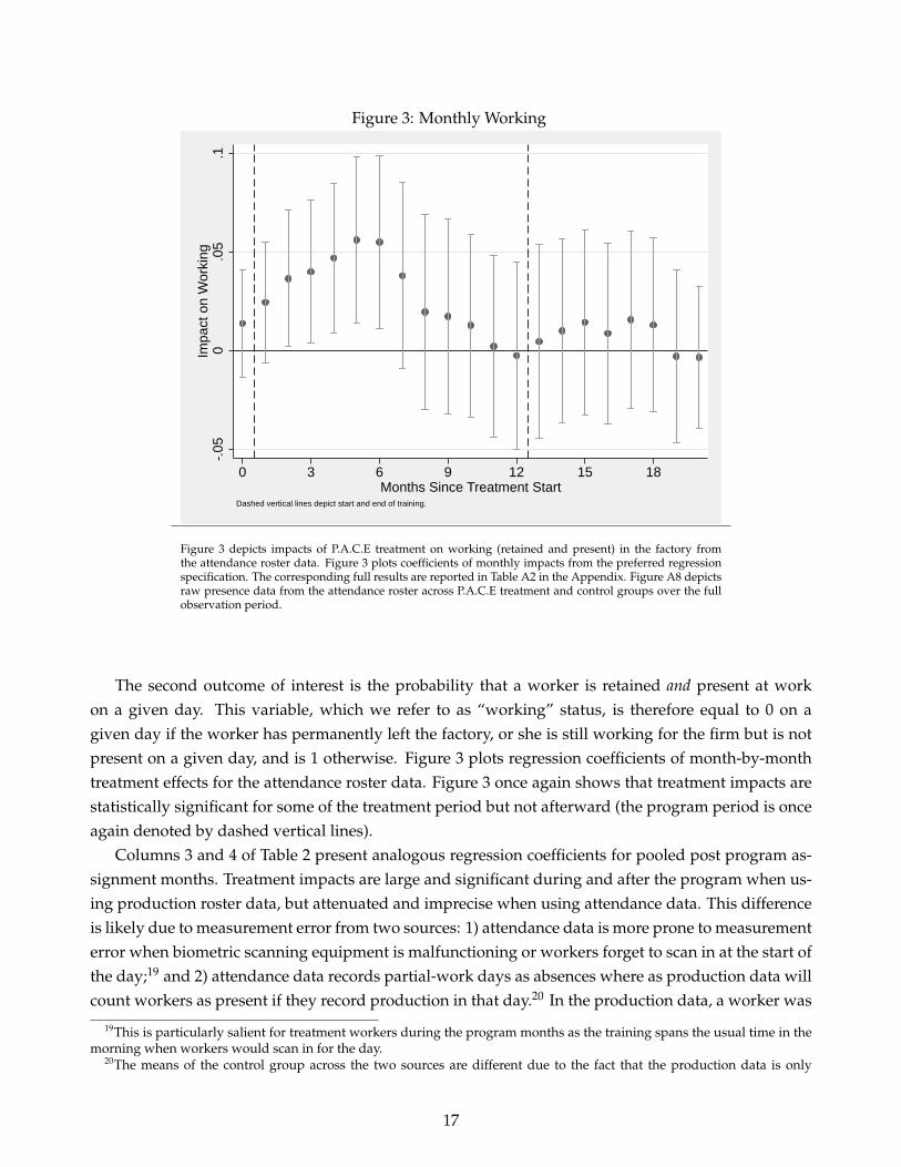
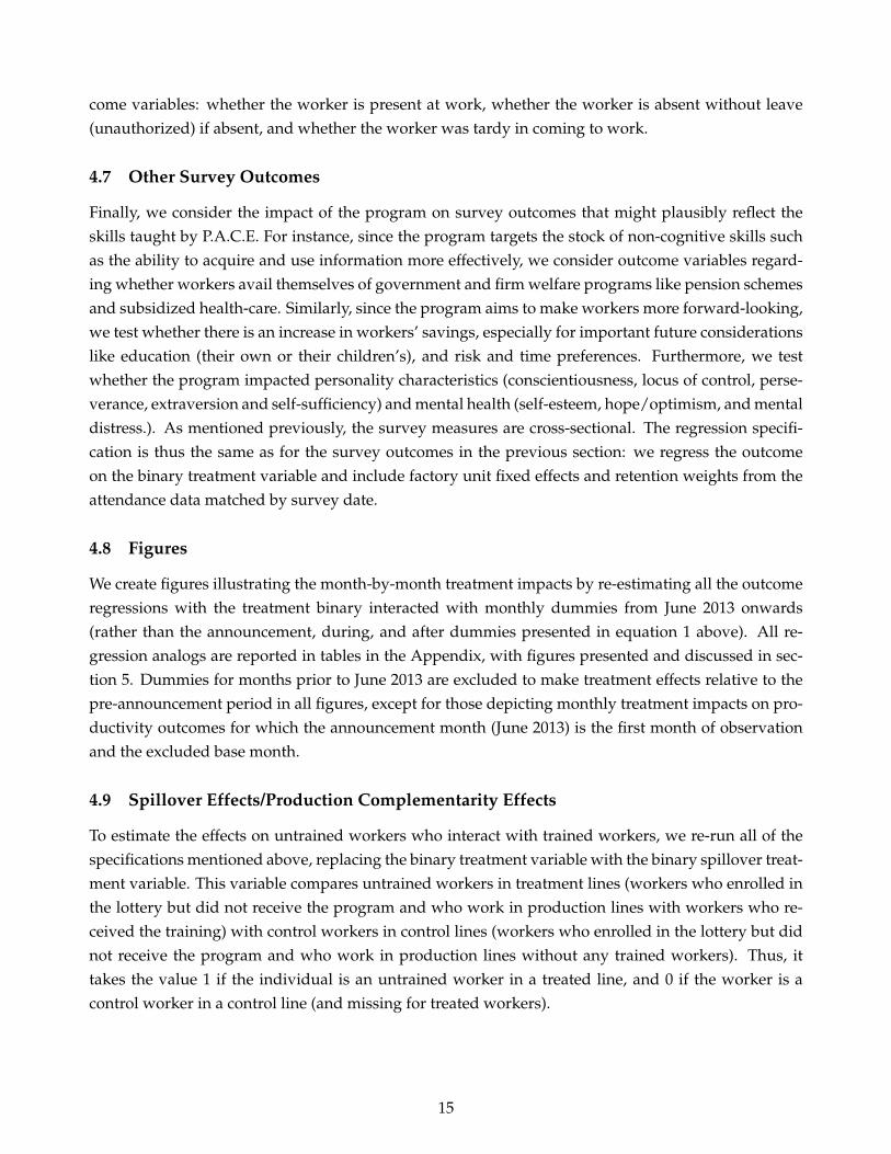
Figure 3: Monthly Working

-.05

0.0

5.1

Impa

ct o

n W

orki

ng



Figure 3 depicts impacts of P.A.C.E treatment on working (retained and present) in the factory fromthe attendance roster data. Figure 3 plots coefficients of monthly impacts from the preferred regressionspecification. The corresponding full results are reported in Table A2 in the Appendix. Figure A8 depictsraw presence data from the attendance roster across P.A.C.E treatment and control groups over the fullobservation period.

The second outcome of interest is the probability that a worker is retained and present at workon a given day. This variable, which we refer to as “working” status, is therefore equal to 0 on agiven day if the worker has permanently left the factory, or she is still working for the firm but is notpresent on a given day, and is 1 otherwise. Figure 3 plots regression coefficients of month-by-monthtreatment effects for the attendance roster data. Figure 3 once again shows that treatment impacts arestatistically significant for some of the treatment period but not afterward (the program period is onceagain denoted by dashed vertical lines).

Columns 3 and 4 of Table 2 present analogous regression coefficients for pooled post program as-signment months. Treatment impacts are large and significant during and after the program when us-ing production roster data, but attenuated and imprecise when using attendance data. This differenceis likely due to measurement error from two sources: 1) attendance data is more prone to measurementerror when biometric scanning equipment is malfunctioning or workers forget to scan in at the start ofthe day;19 and 2) attendance data records partial-work days as absences where as production data willcount workers as present if they record production in that day.20 In the production data, a worker was

19This is particularly salient for treatment workers during the program months as the training spans the usual time in themorning when workers would scan in for the day.

20The means of the control group across the two sources are different due to the fact that the production data is only

17

Table 2: Impacts of P.A.C.E. Treatment on Retention, Working, and Person Days

(1) (2) (3) (4) (5) (6)

Attendance Roster Payroll Roster Attendance Roster Production Data Attendance Roster Production Data

After X P.A.C.E. Treatment 0.00620 0.00865 0.00743 0.0761** 9.250 16.20**(0.0256) (0.0274) (0.0221) (0.0371) (8.683) (7.141)

During X P.A.C.E. Treatment 0.0264 0.0256 0.0285 0.0870*** 5.360 6.833***(0.0215) (0.0220) (0.0193) (0.0318) (3.258) (2.601)

Announced X P.A.C.E.. Treatment 0.00416 0.00476 0.0136 0.501(0.0136) (0.0153) (0.0138) (1.271)

Fixed Effects

Observations 1,433,981 43,141 1,270,871 778,916 1,270,871 778,916Control Mean of Dependent Variable 0.63 0.66 0.52 0.37 213.71 103.22

Cumulative Person Days

Sum of Days Working for Each Worker to Date

Notes: Robust standard errors in parentheses (*** p<0.01, ** p<0.05, * p<0.1). Standard errors are clustered at the treatment line level. Retained dummy, Working dummy, and Cumulative Person Days are all defined for every worker date observation in the data and therfore the regressions do not require any weighting.

Unit X Month X Year, Worker

Retained

1(Worker Still on Attendance Roster)

Working

1(Worker Retained and Present in Factory Today)

8.7 percentage points more likely to be working during the program (a 23.5% increase relative to thecontrol mean) and 7.6 percentage points more likely to be working after the program (a 20% increaserelative to the control mean).

The final measure we study regarding retention and working status is the cumulative number ofworking days that accrue to the firm. This is the running sum of the working status variable justdiscussed. Figure 4 shows that the treatment impact on cumulative person days (calculated fromproduction data) is positive and statistically significant by about 3 months into the program period.The impacts continue to grow quickly through month 8 of the training period, after which the growthslows somewhat but remains positive through the remainder of the observation period. Columns 5and 6 of Table 2 present the impacts on cumulative person days during and after the program, usingattendance and production data, respectively. The treatment increases the cumulative person days pertreated worker by 6.8 days during treatment and 16.2 days after treatment when the production datais used, which is about 6.6% and 16% of the mean cumulative number of days of the control grouprespectively.

5.2 Productivity and Task Complexity

If P.A.C.E. impacted the stock of soft skills (e.g., time management, communication, extraversion), thenit should follow that marginal productivity rises, both through direct channels, to the extent that softskills are used in production, and indirect channels, if workers were more likely to ask for and receiveadditional training in hard skills. To test this hypothesis, we consider two outcomes: 1) productivityas reflected in the industry standard measure of efficiency (pieces produced divided by target pieces);

available starting June 2013 (the month of treatment announcement), so has five months less of data relative to the attendanceroster.

18

Figure 4: Monthly Person Days

010

2030

40Im

pact

on

Cum

ulat

iveP

erso

nDay

s



Figure 4 depicts impacts of P.A.C.E treatment on cumulative person days in the factory from the startof the production data (June 1, 2013) to each date. Figure 4 plots coefficients of monthly impacts fromthe preferred regression specification on the production data. The corresponding full results are reportedin Table A2 in the Appendix. Figure A9 depicts raw person days data from the production data acrossP.A.C.E treatment and control groups over the full observation period.

and 2) the complexity of the task to which workers are assigned, as measured by SAM (number ofminutes in which a task is expected to be completed – a higher SAM thus denotes a more complextask).

Figures 5A and 5B plot regression coefficients of impacts of treatment on efficiency, estimatedmonth by month. Figure 5A presents this for all workers in the sample, and Figure 5B for only thoseworkers who were retained at the end of the data collection period (February 2015). The figures indi-cate that treatment increases efficiency throughout the training and post-program period, with coeffi-cients becoming significant towards the last third of the program period and after. Figures 6A and 6Bplot analogous regression coefficients of monthly treatment impacts on the complexity of the operationthe worker is performing as measured by SAM. These figures illustrate that both during and after theprogram, there is evidence that treated workers are assigned to more complex tasks (tasks with higherSAM).

These patterns are confirmed in Table 3, which reports the results of analogous regressions in whichimpacts are grouped into during and after P.A.C.E. program implementation. Treated workers aremore efficient after the program (relative to the month of treatment assignment announcement) bynearly 11 percentage points, about 20% relative the control group mean. Consistent with the evidencepresented above, we see that the impacts on productivity are stronger after program completion. For

19

Figure 5A: Monthly Efficiency (All Workers)-.1

0.1

.2.3

Impa

ct o

n Ef

ficie

ncy



Figure 5B: Monthly Efficiency (Retained Only)

-.10

.1.2

.3Im

pact

on

Effic

ienc

y



Figures 5A and 5B depict impacts of P.A.C.E treatment on productivity in the factory. Figure 5A depicts coefficients of monthlyimpacts on efficiency (actual pieces produced / target pieces) from the preferred regression specification (including worker by item(style) fixed effects and controls for the number of days the worker has been producing that style on that line and the total orderquantity) for the full sample of workers, with observations weighted to account for any differential composition across treatment andcontrol due to attrition. Figure 5B presents the analogous figure for the subsample of workers who are still retained in the factory bythe end of observation (February 2015). The corresponding full results are reported in Table A3 in the Appendix.

Figure 6A: Monthly SAM (All Workers)

-.05

0.0

5.1

Impa

ct o

n SA

M



Figure 6B: Monthly SAM (Retained Only)

-.1-.0

50

.05

.1.1

5Im

pact

on

SAM



Figures 6A and 6B depict impacts of P.A.C.E treatment on operation complexity (SAM, or standard allowable minute peroperation-piece). Figure 6A depicts coefficients of monthly impacts from the preferred regression specification for all workers.Figure 6B depicts monthly impacts for the subsample of retained workers only. The corresponding full results are reported inTable A3 in the Appendix. Figure A11 depicts raw SAM from the production data across P.A.C.E treatment and control groupsover the full observation period (June 1, 2013 onwards in the production data).

the sub-sample of workers who were retained until the end of the data collection period, the magni-

20

Table 3: Impacts of P.A.C.E. Treatment on Productivity

(1) (2) (3) (4)Efficiency SAM (Operation Complexity) Efficiency SAM (Operation Complexity)

Produced/Target Standard Allowable Minute Produced/Target Standard Allowable Minute

After X P.A.C.E. Treatment 0.108** 0.0384** 0.150** 0.0798***(0.0510) (0.0180) (0.0654) (0.0255)

During X P.A.C.E. Treatment 0.0300 0.0334** 0.0693* 0.0642***(0.0274) (0.0147) (0.0390) (0.0208)

Additional ControlsDays on Same Line-Garment,

Total Order SizeNone

Days on Same Line-Garment, Total Order Size

None

Fixed EffectsUnit X Month X Year, Worker X

GarmentUnit X Month X Year, Worker

Unit X Month X Year, Worker X Garment


Weights

Observations 290,763 290,763 130,187 130,187Control Mean of Dependent Variable 0.542 0.565 0.527 0.588

Notes: Robust standard errors in parentheses (*** p<0.01, ** p<0.05, * p<0.1). Standard errors are clustered at the treatment line level. Observations in columns 1 and 2 are weighted in regressions by the inverse of the predicted probability of working (i.e., not yet attrited and present in the factory with non-missing data) in the sample that day from a probit regression of the working dummy on month by year FE and their interaction with individual and line treatment dummies and baseline variables reported in Table 1. Sample in columns 3 and 4 is restricted to only workers still retained in the factory by the end of observation. All samples are trimmed in these regressions to omit days in which the worker is observed for only a half a production day or less or days in which the worker is observed for more than 2 overtime hours as these are anomalous observations with imprecise production measures. These outliers make up only around 5% of the work-day observations.

Retained Workers Only (still in factory in Feb 2015)

Inverse Predicted Probability from Probit of Working on Treatments X Mo-Yr X Baseline Characteristics

None

tude of the treatment effect is similar, about 15 percentage points higher efficiency after the treatment.Figure A10 presents these coefficients for the whole sample and the subsample of retained workersonly together as well as their confidence intervals to test for statistically differences in every month ofdata collection. We cannot reject that the coefficients are the same in any month. The fact that these re-sults are similar across panels further supports the notion that any changing composition of the samplecan be driving the productivity impacts.

Additionally, we see fairly consistent impacts on task complexity (SAM) throughout the program,and they are sustained and remain statistically significant after the program period. That is, treatedworkers are assigned to more complex tasks both during and after treatment (tasks to which they areassigned are expected to take about 2.3 seconds (0.038 minutes) more, roughly 7% of the control groupmean). Thus, not only are workers in the treatment group assigned to more complex tasks during andafter the program, they are more productive even at these harder tasks once treatment ends. The non-cognitive skills that the program covers (like time management, goal setting, and team work) enhanceworker productivity and the ability to perform complex tasks.

The time pattern of impacts on productivity – insignificant increases during much of the programperiod followed by large, significant increases towards the end of training and afterward – is strikingand deserves additional consideration. The observed pattern could be rationalized in several ways.First, the increase in task complexity discussed above (which happened early on in the program pe-riod) may not captured fully by adjusting the target quantity. More complex tasks may take longer tomaster, creating a drag on efficiency particularly just after task switching occurs. Second, the “incuba-tion period” for productivity impacts in the context of this program, through both direct and indirectchannels mentioned above, is likely long. Learning soft skills to the point that they can be applied

21

in the workplace may take time. Third, Sets of soft skills may be complementary, so that incremen-tal learnings in a given module have a greater impact later in the program. This is consistent withthe structure of the program, which conducted review sessions before graduation to reiterate earliermodules and discuss how to combine the new skills together and apply them in both professional andpersonal situations. Finally, from anecdotal observation, women took several months to become trueparticipants in the group sessions; at the beginning of the program the level of participation, fittingwith the cultural context in which these women live, was quite low.

5.3 Career Advancement

In addition to worker presence and productivity, we study career advancement within the firm. Toestimate the impacts of treatment on career advancement, we consider both whether the worker wasgiven a raise using monthly payroll data as well as worker-reported measures of expectations of pro-motion; whether they recently asked for (and received) skill development training; earned productionincentives; and finally, how they assess their own ability relative to all workers on their productionline, and relative to workers of the same technical skill grade as them. Except for the salary data whichis at the monthly level for each worker, the self-reported measures are from the worker-level surveyconducted in the month of program completion and vary only cross-sectionally.

Figure 7: Monthly Salary

0.0

05.0

1.0

15Im

pact

on

log(

Gro

ss S

alar

y)



Figure 7 depicts coefficients of monthly impacts of P.A.C.E treatment on log(gross salary) from the pre-ferred regression specification. The corresponding full results are reported in Table A3 in the Appendix.

Figure 7 plots regression coefficients of monthly treatment impacts on log gross salary. We see in

22

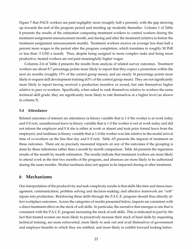
Figure 7 that PACE workers are paid negligibly more (roughly half a percent), with the gap showingup towards the end of the program period and trending up modestly thereafter. Column 1 of Table4 presents the results of the estimation comparing treatment workers to control workers during thetreatment assignment announcement month, and during and after the treatment (relative to before thetreatment assignment announcement month). Treatment workers receive on average less than half apercent more wages in the period after the program completion, which translates to roughly 30 INRor less than .5 USD a month. Thus, despite being assigned to more complex tasks and being moreproductive, treated workers are not paid meaningfully higher wages.

Columns 2-6 of Table 4 presents the results from analysis of related survey outcomes. Treatmentworkers are about 8.7 percentage points more likely to report that they expect a promotion within thenext six months (roughly 15% of the control group mean), and are nearly 16 percentage points morelikely to request skill development training (63% of the control group mean). They are not significantlymore likely to report having received a production incentive or award, but rate themselves higherrelative to peer co-workers. Specifically, when asked to rank themselves relative to workers the sametechnical skill grade, they are significantly more likely to rate themselves at a higher level (as shownin column 5).

5.4 Attendance

Related outcomes of interest are attendance (a binary variable that is 1 if the worker is at work todayand 0 if not), unauthorized leave (a binary variable that is 1 if the worker is not at work today and didnot inform the employer and 0 if she is either at work or absent and took prior formal leave from theemployer), and tardiness (a binary variable that is 1 if the worker was late relative to the modal arrivaltime of co-workers on the line that day and 0 if not). Table A5 presents the impacts of treatment onthese outcomes. There are no precisely measured impacts on any of the outcomes if the grouping isdone by these milestones rather than a month by month comparison. Table A6 presents the regressionresults of the month by month estimation. The results indicate that treatment workers are more likelyto attend work in the first two months of the program, and absences are more likely to be authorizedduring the same months. Worker tardiness does not appear to be impacted during or after treatment.

6 Mechanisms

Our interpretation of the productivity and task complexity results is that skills like time and stress man-agement; communication; problem solving and decision-making; and effective teamwork are “soft”inputs into production. Reinforcing these skills through the P.A.C.E. program should thus directly af-fect workplace outcomes. Across the categories of results presented below, impacts are consistent witha direct treatment effect on the stock of soft skills. In particular, the narrative that emerges is one that isconsistent with the P.A.C.E. program increasing the stock of soft skills. This is indicated in part by thefact that treated women are more likely to proactively increase their stock of hard skills by requestingtechnical training, are more extraverted, more likely to seek out and avail themselves of governmentand employer benefits to which they are entitled, and more likely to exhibit forward looking behav-

23

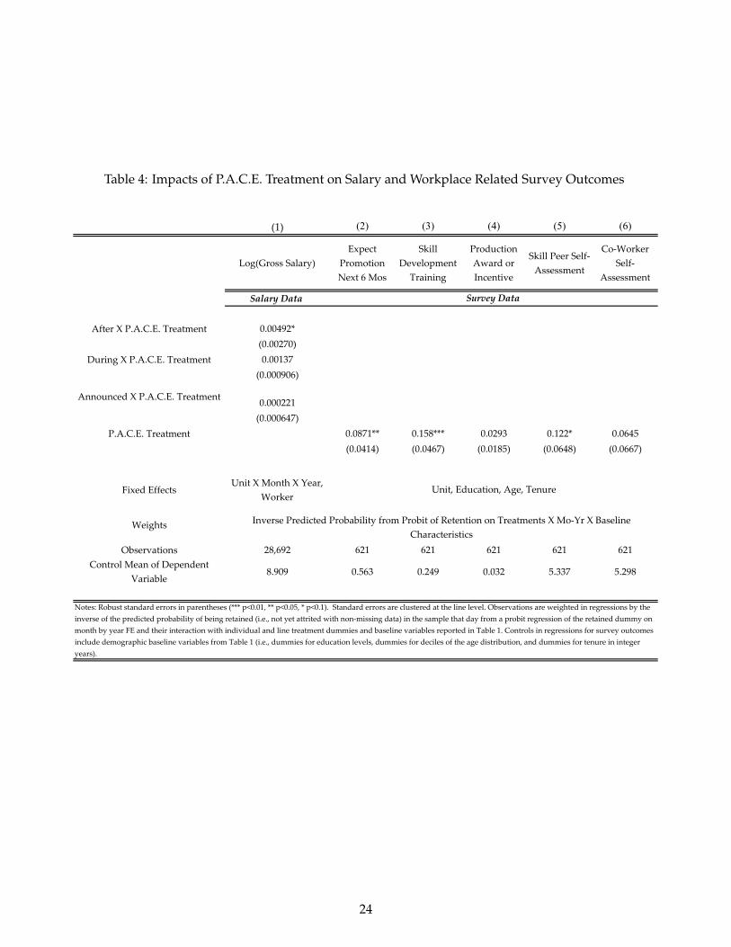
Table 4: Impacts of P.A.C.E. Treatment on Salary and Workplace Related Survey Outcomes

(1) (2) (3) (4) (5) (6)

Log(Gross Salary)Expect

Promotion Next 6 Mos

Skill Development

Training

Production Award or Incentive

Skill Peer Self‐Assessment

Co‐Worker Self‐

Assessment

Salary Data

After X P.A.C.E. Treatment 0.00492*(0.00270)

During X P.A.C.E. Treatment 0.00137(0.000906)

Announced X P.A.C.E. Treatment 0.000221(0.000647)

P.A.C.E. Treatment 0.0871** 0.158*** 0.0293 0.122* 0.0645(0.0414) (0.0467) (0.0185) (0.0648) (0.0667)

Fixed EffectsUnit X Month X Year,

Worker

Weights

Observations 28,692 621 621 621 621 621Control Mean of Dependent

Variable8.909 0.563 0.249 0.032 5.337 5.298

Inverse Predicted Probability from Probit of Retention on Treatments X Mo‐Yr X Baseline Characteristics

Notes: Robust standard errors in parentheses (*** p<0.01, ** p<0.05, * p<0.1). Standard errors are clustered at the line level. Observations are weighted in regressions by the inverse of the predicted probability of being retained (i.e., not yet attrited with non‐missing data) in the sample that day from a probit regression of the retained dummy on month by year FE and their interaction with individual and line treatment dummies and baseline variables reported in Table 1. Controls in regressions for survey outcomes include demographic baseline variables from Table 1 (i.e., dummies for education levels, dummies for deciles of the age distribution, and dummies for tenure in integer years).

Unit, Education, Age, Tenure

Survey Data

24

ior via savings and aspirations for their children’s future. Finally, these women share learnings withtheir untrained co-workers, and these spillovers appear to contribute to the productivity of these co-workers.

Below, we support this interpretation using evidence from a survey of treatment and control work-ers; from assessments of the treatment group’s knowledge before and after the completion of the pro-gram’s core modules; and from the degree of treatment spillovers. We also present several alternativeinterpretations and discuss the plausibility of each in turn.

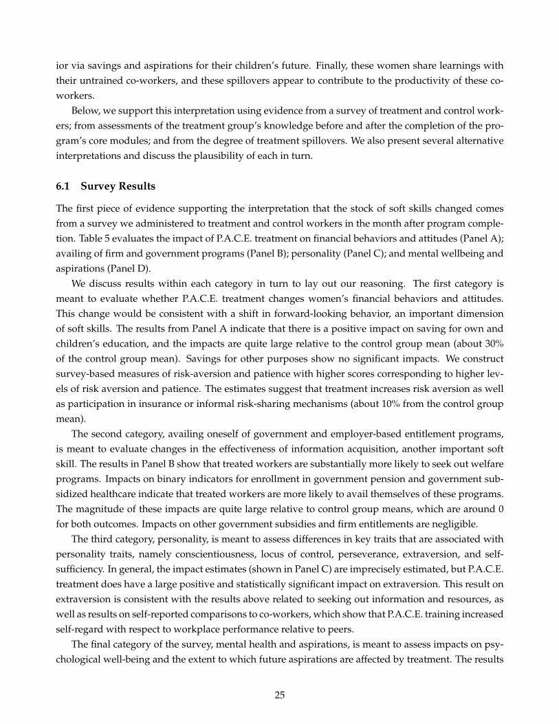
6.1 Survey Results

The first piece of evidence supporting the interpretation that the stock of soft skills changed comesfrom a survey we administered to treatment and control workers in the month after program comple-tion. Table 5 evaluates the impact of P.A.C.E. treatment on financial behaviors and attitudes (Panel A);availing of firm and government programs (Panel B); personality (Panel C); and mental wellbeing andaspirations (Panel D).

We discuss results within each category in turn to lay out our reasoning. The first category ismeant to evaluate whether P.A.C.E. treatment changes women’s financial behaviors and attitudes.This change would be consistent with a shift in forward-looking behavior, an important dimensionof soft skills. The results from Panel A indicate that there is a positive impact on saving for own andchildren’s education, and the impacts are quite large relative to the control group mean (about 30%of the control group mean). Savings for other purposes show no significant impacts. We constructsurvey-based measures of risk-aversion and patience with higher scores corresponding to higher lev-els of risk aversion and patience. The estimates suggest that treatment increases risk aversion as wellas participation in insurance or informal risk-sharing mechanisms (about 10% from the control groupmean).

The second category, availing oneself of government and employer-based entitlement programs,is meant to evaluate changes in the effectiveness of information acquisition, another important softskill. The results in Panel B show that treated workers are substantially more likely to seek out welfareprograms. Impacts on binary indicators for enrollment in government pension and government sub-sidized healthcare indicate that treated workers are more likely to avail themselves of these programs.The magnitude of these impacts are quite large relative to control group means, which are around 0for both outcomes. Impacts on other government subsidies and firm entitlements are negligible.

The third category, personality, is meant to assess differences in key traits that are associated withpersonality traits, namely conscientiousness, locus of control, perseverance, extraversion, and self-sufficiency. In general, the impact estimates (shown in Panel C) are imprecisely estimated, but P.A.C.E.treatment does have a large positive and statistically significant impact on extraversion. This result onextraversion is consistent with the results above related to seeking out information and resources, aswell as results on self-reported comparisons to co-workers, which show that P.A.C.E. training increasedself-regard with respect to workplace performance relative to peers.

The final category of the survey, mental health and aspirations, is meant to assess impacts on psy-chological well-being and the extent to which future aspirations are affected by treatment. The results

25

Table 5: Impacts of P.A.C.E. Treatment on Survey Outcomes

(1) (2) (3) (4) (5)

Panel A: Financial Behaviors and Attitudes Saving for EducationSaving for Other

ReasonsRisk Preference

IndexTime Preference

Index

Insurance or Informal Risk-

Sharing

P.A.C.E. Treatment 0.0804** -0.0465 0.166* -0.0984 0.0637*(0.0313) (0.0334) (0.0876) (0.0935) (0.0351)

Control Group Mean of Dependent Variable 0.265 0.272 -0.052 0.019 0.628

Panel B: Government and Firm Entitlements Gov. PensionGov. Subsidized

HealthcareOther Gov. Subsidy Firm Entitlements

Community Self Help Group

P.A.C.E. Treatment 0.0248* 0.0226** 0.0119 -0.0257 -0.0270(0.0141) (0.00941) (0.0310) (0.0352) (0.0303)

Control Group Mean of Dependent Variable 0.039 0.006 0.120 0.142 0.152

Panel C: Personality Conscientiousness Locus of Control Perserverance Extraversion Self-Sufficiency

P.A.C.E. Treatment 0.0210 0.0307 -0.123 0.164** 0.0445(0.0732) (0.0770) (0.0774) (0.0702) (0.0877)

Control Group Mean of Dependent Variable -0.047 -0.040 0.020 -0.071 -0.063

Panel D: Mental Health and Aspirations Self-Esteem Hope/Optimism Moderate DistressChild's Expected Age at Marriage

Child Educated Beyond College

P.A.C.E. Treatment -0.172 -0.0621 -0.0422 0.0456 0.0885***(0.106) (0.0819) (0.0389) (0.165) (0.0280)

Control Group Mean of Dependent Variable 0.048 0.015 0.094 23.427 0.117

Fixed EffectsWeighted

Observations 621 621 621 621 621

Notes: Robust standard errors in parentheses (*** p<0.01, ** p<0.05, * p<0.1). Standard errors are clustered at the treatment line level. Obersvations are weighted in regressions by the inverse of the predicted probability of being retained (i.e., not yet attrited with non-missing data) in the sample that day from a probit regression in the attendance roster of the retained dummy on month by year FE and their interaction with individual and line treatment dummies and baseline variables reported in Table 1. Controls include demograhpic baseline variables from Table 1 (i.e., dummies for education levels, dummies for deciles of age distribution, and dummies for tenure in integer years).

Inverse Predicted Probability from Probit of Retention on Treatments X Baseline CharacteristicsUnit, Education, Age, Tenure

26

reported in Panel D show that, in general, outcomes associated with psychological well-being (self-esteem, optimism, and mental distress) are unaffected by P.A.C.E. treatment, but aspirations for chil-dren’s education rise dramatically in relation to the control group mean. This is consistent with theresult on saving for education presented in Panel A.

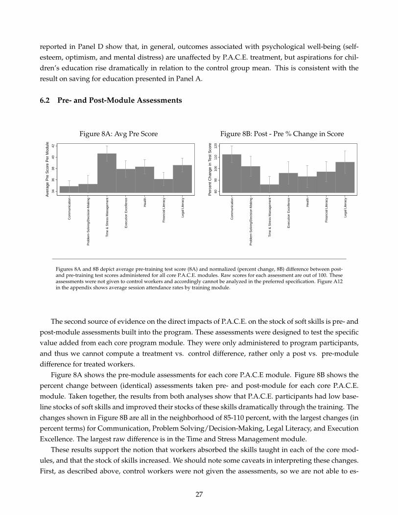
6.2 Pre- and Post-Module Assessments

Figure 8A: Avg Pre Score

3436

3840

42Av

erag

e Pr

e Sc

ore

Per M

odul

e

Com

mun

icat

ion

Prob

lem

-Sol

ving

/Dec

isio

n-M

akin

g

Tim

e &

Stre

ss M

anag

emen

t

Exec

utio

n Ex

celle

nce

Hea

lth

Fina

ncia

l Lite

racy

Lega

l Lite

racy

Figure 8B: Post - Pre % Change in Score

8090

100

110

120

Perc

ent C

hang

e in

Tes

t Sco

re

Com

mun

icat

ion

Prob

lem

-Sol

ving

/Dec

isio

n-M

akin

g

Tim

e &

Stre

ss M

anag

emen

t

Exec

utio

n Ex

celle

nce

Hea

lth

Fina

ncia

l Lite

racy

Lega

l Lite

racy

Figures 8A and 8B depict average pre-training test score (8A) and normalized (percent change, 8B) difference between post-and pre-training test scores administered for all core P.A.C.E. modules. Raw scores for each assessment are out of 100. Theseassessments were not given to control workers and accordingly cannot be analyzed in the preferred specification. Figure A12in the appendix shows average session attendance rates by training module.

The second source of evidence on the direct impacts of P.A.C.E. on the stock of soft skills is pre- andpost-module assessments built into the program. These assessments were designed to test the specificvalue added from each core program module. They were only administered to program participants,and thus we cannot compute a treatment vs. control difference, rather only a post vs. pre-moduledifference for treated workers.

Figure 8A shows the pre-module assessments for each core P.A.C.E module. Figure 8B shows thepercent change between (identical) assessments taken pre- and post-module for each core P.A.C.E.module. Taken together, the results from both analyses show that P.A.C.E. participants had low base-line stocks of soft skills and improved their stocks of these skills dramatically through the training. Thechanges shown in Figure 8B are all in the neighborhood of 85-110 percent, with the largest changes (inpercent terms) for Communication, Problem Solving/Decision-Making, Legal Literacy, and ExecutionExcellence. The largest raw difference is in the Time and Stress Management module.

These results support the notion that workers absorbed the skills taught in each of the core mod-ules, and that the stock of skills increased. We should note some caveats in interpreting these changes.First, as described above, control workers were not given the assessments, so we are not able to es-

27

timate impacts by comparing across the treatment and control groups). Second, we are measuringskill retention directly after module completion; this does not necessarily reflect long-term skill reten-tion. Nevertheless, these results are consistent with our hypothesis that P.A.C.E. acted on workplaceoutcomes by increasing the stock of soft skills.

6.3 Treatment Spillovers

Finally, we consider evidence on spillovers. Recall that the experiment was designed to capturespillovers within production lines through a two-stage randomization procedure, in which lines werefirst randomized to treatment or control, and then within treatment lines, workers who had enrolled inthe P.A.C.E. lottery were randomized to treatment or to the spillover group. In this section we evaluatespillovers by comparing the outcomes of this latter group to control workers on control lines. The ex-istence of spillovers would provide greater justification for employer investment in soft skills training.We evaluate these hypotheses in Table 6, which presents the spillover results for workplace outcomesof interest.21

Panel A presents the results for person days as well as productivity. There is a weakly statisti-cally significant impact on the binary for working during the treatment announcement period, and astronger result for cumulative person days during the treatment period - untrained workers who workwith treated workers work for about 8 more days during program months relative to control workers.Productivity impacts are positive, about 70% as large as the direct treatment effects, but are not statis-tically significant. Panel B presents the results for career advancement variables. Similar to the effecton productivity, the spillover impacts on survey outcomes on requesting skill development training,receiving a production incentive or self-assessment relative to co-workers are not precisely measured,but again have coefficients of the same sign as the main treatment impacts. The worker self-assessmentrelative to co-workers is positive and statistically significant at the 10% level.

Table A8 presents the results for the non-workplace outcomes of interest for spillovers. On thewhole, estimates for non-workplace outcomes do not show a strong pattern of spillover impacts.However, like directly trained workers, spillover workers are also more likely to be saving for theirchildrens’ education and utilizing government subsidized healthcare.

In sum, then, for workplace outcomes we see large spillover impacts on cumulative person daysaccrued to the firm, and imprecisely estimated but positive effects on efficiency. We see some evidencefor spillovers on outcomes outside the workplace, but the results are imprecise in general. Overall,the presence of spillovers suggests that knowledge transfer happened as a direct result of the program– i.e., that program participants imbibed soft skills, which they then communicated to co-workers ontheir production lines, and that transfer helped improve outcomes of non-participants, as well.

6.4 Alternative Mechanisms

Having presented evidence on the salience of direct skilling as a result of the P.A.C.E. program, wenow discuss several alternative interpretations of the results and any supporting evidence of each.

21Note that probability weights, when necessary, are calculated exactly as they are in the treatment effect estimation, usingspillover treatment indicators in place of direct P.A.C.E. training.

28

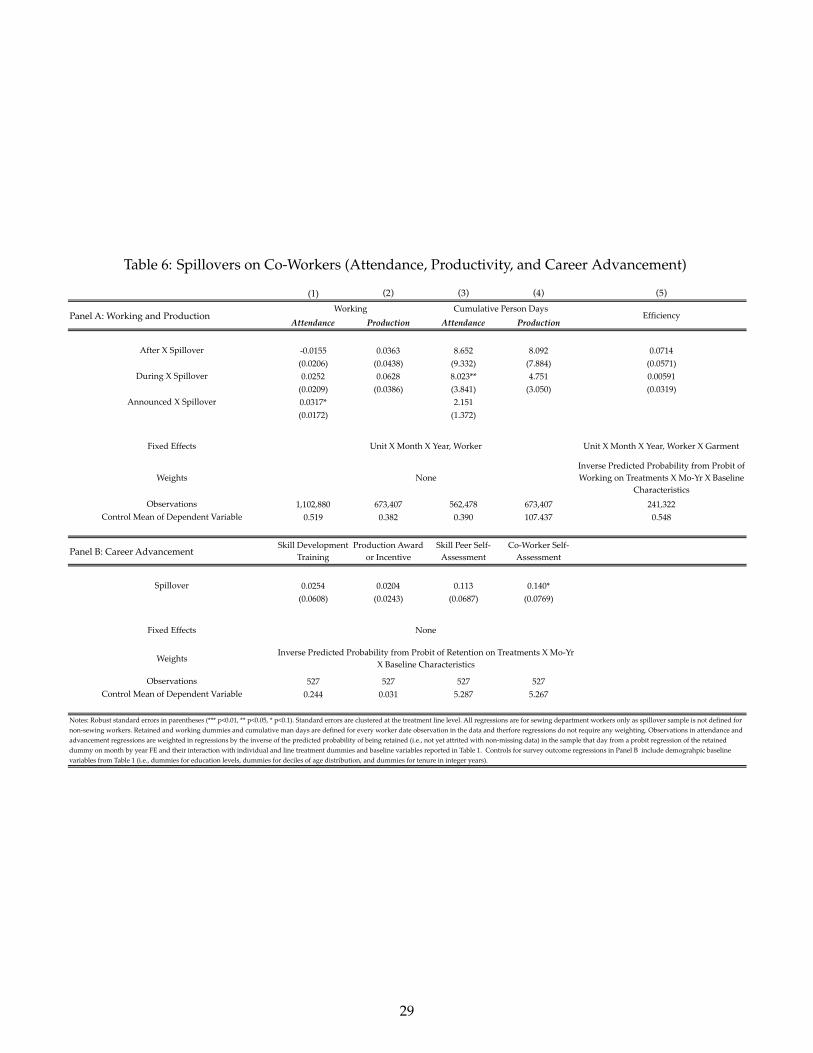
Table 6: Spillovers on Co-Workers (Attendance, Productivity, and Career Advancement)

(1) (2) (3) (4) (5)

Attendance Production Attendance Production

After X Spillover -0.0155 0.0363 8.652 8.092 0.0714(0.0206) (0.0438) (9.332) (7.884) (0.0571)

During X Spillover 0.0252 0.0628 8.023** 4.751 0.00591(0.0209) (0.0386) (3.841) (3.050) (0.0319)

Announced X Spillover 0.0317* 2.151(0.0172) (1.372)

Fixed Effects Unit X Month X Year, Worker X Garment

WeightsInverse Predicted Probability from Probit of Working on Treatments X Mo-Yr X Baseline

CharacteristicsObservations 1,102,880 673,407 562,478 673,407 241,322

Control Mean of Dependent Variable 0.519 0.382 0.390 107.437 0.548

Panel B: Career AdvancementSkill Development

TrainingProduction Award

or IncentiveSkill Peer Self-

AssessmentCo-Worker Self-

Assessment

Spillover 0.0254 0.0204 0.113 0.140*(0.0608) (0.0243) (0.0687) (0.0769)

Fixed Effects

Weights

Observations 527 527 527 527Control Mean of Dependent Variable 0.244 0.031 5.287 5.267

Notes: Robust standard errors in parentheses (*** p<0.01, ** p<0.05, * p<0.1). Standard errors are clustered at the treatment line level. All regressions are for sewing department workers only as spillover sample is not defined for non-sewing workers. Retained and working dummies and cumulative man days are defined for every worker date observation in the data and therfore regressions do not require any weighting. Observations in attendance and advancement regressions are weighted in regressions by the inverse of the predicted probability of being retained (i.e., not yet attrited with non-missing data) in the sample that day from a probit regression of the retained dummy on month by year FE and their interaction with individual and line treatment dummies and baseline variables reported in Table 1. Controls for survey outcome regressions in Panel B include demograhpic baseline variables from Table 1 (i.e., dummies for education levels, dummies for deciles of age distribution, and dummies for tenure in integer years).

Inverse Predicted Probability from Probit of Retention on Treatments X Mo-Yr X Baseline Characteristics

None

None


Panel A: Working and ProductionWorking Cumulative Person Days

Efficiency

29

First, we address the potential importance of reciprocity (an impulse to give back to the employeras a result of access to the program). While it is plausible that some part of the impacts observed isdue to reciprocity, we deem it unlikely that the majority of impacts are due to this mechanism. Thisis for two reasons. First, we find spillovers in treatment for the number of days worked by workerswho were signed up for the program and were on the same production line as treatment workers, butdid not receive the program. These would be difficult to explain if reciprocity were the main drivingforce behind workplace impacts, since non-participants should not be driven by this motive. Second,productivity impacts accumulate slowly during the program period and persist strongly for at least 8months after program completion, with the largest productivity impacts occurring during this post-training period. This does not fit well with a reciprocity motive as a primary mechanism, since wewould expect the reciprocity motive to be strongest while the program is offered and to dissipate overtime if pay does not rise commensurately with productivity as in this case. This indirect evidence isin line with recent, more direct tests of the role of reciprocity in workplace settings (DellaVigna et al.,2016).

Second, we evaluate the possibility that the results for productivity and task complexity were dueto sheepskin effects, i.e., taking part in P.A.C.E. “certified” workers as high quality from the perspectiveof management, and this led to the improvements in workplace outcomes we observe. We reason thatsheepskin effects are unlikely to explain the majority of the program’s impacts given the slow onset ofincreased productivity over time, rather than an increase near the program’s end. Additionally, onceagain spillover impacts are inconsistent with a sheepskin effect mechanism.

Third, it is possible that workers found the classes enjoyable and they improved workers’ subjectivewellbeing, which in turn made workers more productive. The results reported in Panel D in Table 5show that levels of psychological distress are unaffected by treatment, which contradict changes inworker well-being and happiness being the mechanism for productivity impacts.22

Finally, we evaluate the idea that increased social capital drives the results on workplace impacts.The argument here is that it is possible that P.A.C.E. sessions improved the ability of workers to createsocial ties, which could generate higher productivity on their production lines if it increased the extentor intensity of social connectivity on the line. We argue that the context in which the study was runlikely precludes this from being a primary mechanism of impact. First, language-based and culturalbarriers are quite salient in the workplace in our context, likely limiting the extent of the importanceof social connectivity in productivity. Nearly half the workers in the factories under study are mi-grants, many of whom do not speak Kannada, the indigenous language of Karnataka. Second, dueto throughput constraints which dictated the number of workers from the same production line whocould leave at the same time for a P.A.C.E. session, co-workers on the same line were placed in differentsessions conducted on different days of the week. Again, this likely limited the increase in within-linesocial connectivity. These explanations do not preclude overall social ties from being impacted by theprogram; they simply lower the likelihood that this channel contributed significantly to impacts onworkplace outcomes like productivity.

22Results are unchanged if severe mental distress is used as an outcome instead of moderate mental distress.

30

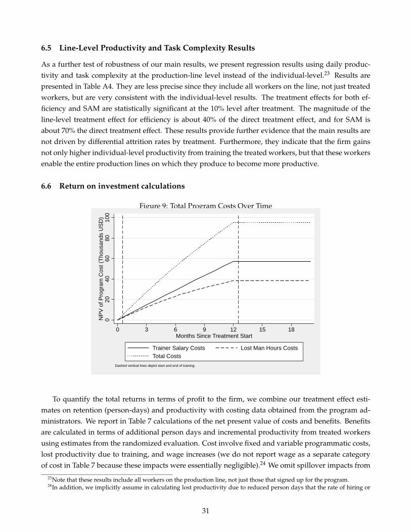
6.5 Line-Level Productivity and Task Complexity Results

As a further test of robustness of our main results, we present regression results using daily produc-tivity and task complexity at the production-line level instead of the individual-level.23 Results arepresented in Table A4. They are less precise since they include all workers on the line, not just treatedworkers, but are very consistent with the individual-level results. The treatment effects for both ef-ficiency and SAM are statistically significant at the 10% level after treatment. The magnitude of theline-level treatment effect for efficiency is about 40% of the direct treatment effect, and for SAM isabout 70% the direct treatment effect. These results provide further evidence that the main results arenot driven by differential attrition rates by treatment. Furthermore, they indicate that the firm gainsnot only higher individual-level productivity from training the treated workers, but that these workersenable the entire production lines on which they produce to become more productive.

6.6 Return on investment calculations

Figure 9: Total Program Costs Over Time

020

4060

8010

0N

PV o

f Pro

gram

Cos

t (Th

ousa

nds

USD

)


Trainer Salary Costs Lost Man Hours CostsTotal Costs


To quantify the total returns in terms of profit to the firm, we combine our treatment effect esti-mates on retention (person-days) and productivity with costing data obtained from the program ad-ministrators. We report in Table 7 calculations of the net present value of costs and benefits. Benefitsare calculated in terms of additional person days and incremental productivity from treated workersusing estimates from the randomized evaluation. Cost involve fixed and variable programmatic costs,lost productivity due to training, and wage increases (we do not report wage as a separate categoryof cost in Table 7 because these impacts were essentially negligible).24 We omit spillover impacts from

23Note that these results include all workers on the production line, not just those that signed up for the program.24In addition, we implicitly assume in calculating lost productivity due to reduced person days that the rate of hiring or

31

the calculations that follow to produce conservative estimates, given that the effects on productivityare not statistically significant.

Figure 10: Cumulative Program Benefits Over Time

010

020

030

040

0N

PV o

f Pro

gram

Ben

efits

(Tho

usan

ds U

SD)


Total Costs Additional Man DaysAdditional Productivity Total Benefits


Table 7 first outlines costs of the program, both overhead costs and variable costs. The overheadcosts are given by the costs of hiring two full-time trainers per factory for the 12 months of the program,additional support time from HR personnel, printed materials, food, and equipment (e.g., PA system).The variable costs are from lost production hours, and the marginal increase in wages for treatedworkers. For the 1087 treated workers, total program costs are approximately $95,000, about $57,000of which are overhead costs, and the remainder variable costs. The time path of total costs in netpresent value (NPV) is shown in Figure 9, with total costs rising linearly during the program periodand peaking at program completion.

Details on profit margins on additional revenue both from an additional person day and additionalproductivity, as well as additional revenue per garment were obtained from the firm. The benefits ofthe program are generated by the higher number of cumulative person days accrued to the firm andby higher worker productivity. At the end of the program period, the NPV of these benefits is just over$164,000, about $52,000 of which is the result of additional person days gained during the programand the rest due to productivity gains. At the end of our tracking period (8 months after programcompletion), total benefits are substantially higher, more than $341,000. In the post-program period,returns via productivity gains dominate, accounting for more than 70% of the total benefits. Figure 10plots the time path of cumulative benefits to the firm. Note that these returns accrued net of attrition

worker replacement is common across treatment and control lines such that differential attrition produces truly lost persondays. This is largely true as hiring is centralized for each factory unit. Accordingly, firm management reported to us that itis impossible for the rate of recruitment, hiring, and training to respond to differential turnover across lines within factoryunit.

32

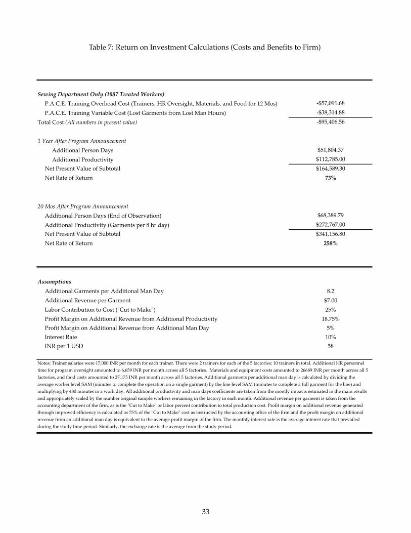
Table 7: Return on Investment Calculations (Costs and Benefits to Firm)

Sewing Department Only (1087 Treated Workers) P.A.C.E. Training Overhead Cost (Trainers, HR Oversight, Materials, and Food for 12 Mos) ‐$57,091.68

P.A.C.E. Training Variable Cost (Lost Garments from Lost Man Hours) ‐$38,314.88

Total Cost (All numbers in present value) ‐$95,406.56

1 Year After Program Announcement

Additional Person Days $51,804.37

Additional Productivity $112,785.00 Net Present Value of Subtotal $164,589.30 Net Rate of Return 73%

20 Mos After Program Announcement

Additional Person Days (End of Observation) $68,389.79

Additional Productivity (Garments per 8 hr day) $272,767.00 Net Present Value of Subtotal $341,156.80 Net Rate of Return 258%

Assumptions

Additional Garments per Additional Man Day 8.2 Additional Revenue per Garment $7.00 Labor Contribution to Cost (ʺCut to Makeʺ) 25% Profit Margin on Additional Revenue from Additional Productivity 18.75% Profit Margin on Additional Revenue from Additional Man Day 5% Interest Rate 10% INR per 1 USD 58

Notes: Trainer salaries were 17,000 INR per month for each trainer. There were 2 trainers for each of the 5 factories; 10 trainers in total. Additional HR personnel time for program oversight amounted to 6,659 INR per month across all 5 factories. Materials and equipment costs amounted to 26689 INR per month across all 5 factories, and food costs amounted to 27,175 INR per month across all 5 factories. Additional garments per additional man day is calculated by dividing the average worker level SAM (minutes to complete the operation on a single garment) by the line level SAM (minutes to complete a full garment for the line) and multiplying by 480 minutes in a work day. All additional productivity and man days coefficients are taken from the montly impacts estimated in the main results and appropriately scaled by the number original sample workers remaining in the factory in each month. Additional revenue per garment is taken from the accounting department of the firm, as is the ʺCut to Makeʺ or labor percent contribution to total production cost. Profit margin on additional revenue generated through improved efficiency is calculated as 75% of the ʺCut to Makeʺ cost as instructed by the accounting office of the firm and the profit margin on additional revenue from an additional man day is equivalent to the average profit margin of the firm. The monthly interest rate is the average interest rate that prevailed during the study time period. Similarly, the exchange rate is the average from the study period.

33

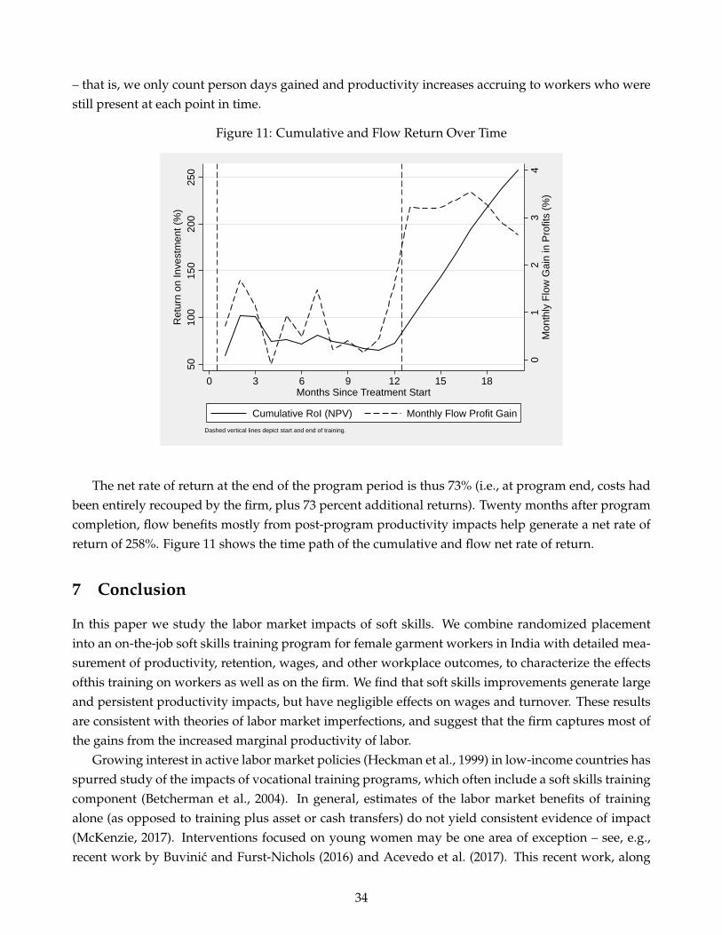
– that is, we only count person days gained and productivity increases accruing to workers who werestill present at each point in time.

Figure 11: Cumulative and Flow Return Over Time

01

23

4M

onth

ly F

low

Gai

n in

Pro

fits

(%)

5010

015

020

025

0R

etur

n on

Inve

stm

ent (

%)


Cumulative RoI (NPV) Monthly Flow Profit GainDashed vertical lines depict start and end of training.

The net rate of return at the end of the program period is thus 73% (i.e., at program end, costs hadbeen entirely recouped by the firm, plus 73 percent additional returns). Twenty months after programcompletion, flow benefits mostly from post-program productivity impacts help generate a net rate ofreturn of 258%. Figure 11 shows the time path of the cumulative and flow net rate of return.

7 Conclusion

In this paper we study the labor market impacts of soft skills. We combine randomized placementinto an on-the-job soft skills training program for female garment workers in India with detailed mea-surement of productivity, retention, wages, and other workplace outcomes, to characterize the effectsofthis training on workers as well as on the firm. We find that soft skills improvements generate largeand persistent productivity impacts, but have negligible effects on wages and turnover. These resultsare consistent with theories of labor market imperfections, and suggest that the firm captures most ofthe gains from the increased marginal productivity of labor.

Growing interest in active labor market policies (Heckman et al., 1999) in low-income countries hasspurred study of the impacts of vocational training programs, which often include a soft skills trainingcomponent (Betcherman et al., 2004). In general, estimates of the labor market benefits of trainingalone (as opposed to training plus asset or cash transfers) do not yield consistent evidence of impact(McKenzie, 2017). Interventions focused on young women may be one area of exception – see, e.g.,recent work by Buvinic and Furst-Nichols (2016) and Acevedo et al. (2017). This recent work, along

34

with our findings, may pave the way for greater concentration on active labor market interventionsfocused on women workers.

Finally, our work is relevant to the literature on female labor force participation (LFP) and employ-ment outcomes, particularly in low-income country contexts (Heath and Jayachandran, 2016). Thispolicy question of how to increase the LFP and career growth of women is especially salient in In-dia, where the level of female LFP is not only unusually low considering India’s level of development(India ranks 120th out of 131 countries in female LFP (Chatterjee et al., 2015)), but has substantiallydecreased in rural areas between 1987 and 2009, despite a fertility transition and relatively robust eco-nomic growth (Afridi et al., 2016). Studying improvements in career prospects for women, via man-agerial training and promotion as Macchiavello et al. (2015) do, or via soft-skills training and resultingproductivity enhancements as we do, can contribute to our understanding of determinants of femalelabor force participation that are amenable to policy intervention.

35

References

Acemoglu, D. (1997). Training and innovation in an imperfect labour market. The Review of EconomicStudies, 64(3):445–464.

Acemoglu, D. and Pischke, J.-S. (1998). Why do firms train? theory and evidence. The Quarterly Journalof Economics, 113(1):79–119.

Acemoglu, D. and Pischke, J.-S. (1999). Beyond becker: training in imperfect labour markets. TheEconomic Journal, 109(453):112–142.

Acevedo, P., Cruces, G., Gertler, P., and Martinez, S. (2017). Living up to expectations: How job trainingmade women better off and men worse off. Technical report, National Bureau of Economic Research.

Afridi, F., Dinkelman, T., and Mahajan, K. (2016). Why are fewer married women joining the workforce in india? a decomposition analysis over two decades.

Aizer, A. and Cunha, F. (2012). The production of child human capital: Endowments, investments andfertility. Unpublished paper, Brown University.

Altonji, J. G. and Spletzer, J. R. (1991). Worker characteristics, job characteristics, and the receipt ofon-the-job training. Industrial & Labor Relations Review, 45(1):58–79.

Anderson, M. L. (2008). Multiple inference and gender differences in the effects of early intervention: Areevaluation of the abecedarian, perry preschool, and early training projects. Journal of the AmericanStatistical Association, pages 1481–1495.

Ashraf, N., Low, C., and McGinn, K. (2017). Negotiating a better future: Communication skills andinter-generational investment in zambia. Technical report, mimeo.

Attanasio, O. P., Fernandez, C., Fitzsimons, E. O., Grantham-McGregor, S. M., Meghir, C., and Rubio-Codina, M. (2014). Using the infrastructure of a conditional cash transfer program to deliver ascalable integrated early child development program in colombia: cluster randomized controlledtrial. BMJ, 349:g5785.

Autor, D. H. (2001). Why do temporary help firms provide free general skills training? QuarterlyJournal of Economics, pages 1409–1448.

Barrett, A. and O’Connell, P. J. (2001). Does training generally work? the returns to in-companytraining. Industrial & labor relations review, 54(3):647–662.

Barron, J. M., Berger, M. C., and Black, D. A. (1999). Do workers pay for on-the-job training? Journal ofHuman Resources, pages 235–252.

Bartel, A. P. and Sicherman, N. (1998). Technological change and the skill acquisition of young workers.Journal of Labor Economics, 16(4):718–55.

36

Bassanini, A., Booth, A., Brunello, G., De Paola, M., Leuven, E., et al. (2007). Workplace training ineurope. Education and Training in Europe.

Bassi, V., Nansamba, A., and Liberia, B. (2017). Information frictions in the labor market: Evidencefrom a field experiment in uganda. Technical report, mimeo.

Becker, G. S. (1964). Human capital.

Benjamini, Y. and Hochberg, Y. (1995). Controlling the false discovery rate: a practical and powerfulapproach to multiple testing. Journal of the royal statistical society. Series B (Methodological), pages289–300.

Betcherman, G., Dar, A., and Olivas, K. (2004). Impacts of active labor market programs: New evidencefrom evaluations with particular attention to developing and transition countries. Social Protection, WorldBank.

Blundell, R., Dearden, L., Meghir, C., and Sianesi, B. (1999). Human capital investment: the returnsfrom education and training to the individual, the firm and the economy. Fiscal studies, 20(1):1–23.

Borghans, L., Duckworth, A. L., Heckman, J. J., and Ter Weel, B. (2008). The economics and psychologyof personality traits. Journal of human Resources, 43(4):972–1059.

Buvinic, M. and Furst-Nichols, R. (2016). Promoting women’s economic empowerment: what works?The World Bank Research Observer, 31(1):59–101.

Campos, F., Frese, M., Goldstein, M., Iacovone, L., Johnson, H. C., McKenzie, D., and Mensmann,M. (2017). Teaching personal initiative beats traditional training in boosting small business in westafrica. Science, 357(6357):1287–1290.

Chang, C. and Wang, Y. (1996). Human capital investment under asymmetric information: The pigo-vian conjecture revisited. Journal of Labor Economics, pages 505–519.

Chatterjee, U., Murgai, R., and Rama, M. (2015). Job opportunities along the rural-urban gradationand female labor force participation in india. World Bank Policy Research Working Paper, (7412).

Cunha, F., Heckman, J. J., and Schennach, S. M. (2010). Estimating the technology of cognitive andnoncognitive skill formation. Econometrica, 78(3):883–931.

Cunningham, W. V. and Villasenor, P. (2016). Employer voices, employer demands, and implicationsfor public skills development policy connecting the labor and education sectors. The World BankResearch Observer, 31(1):102–134.

Dearden, L., Reed, H., and Van Reenen, J. (2006). The impact of training on productivity and wages:Evidence from british panel data. Oxford bulletin of economics and statistics, 68(4):397–421.

DellaVigna, S., List, J. A., Malmendier, U., and Rao, G. (2016). Estimating social preferences and giftexchange at work. Technical report, National Bureau of Economic Research.

37

Deming, D. J. (2015). The growing importance of social skills in the labor market. Technical report,National Bureau of Economic Research.

Gertler, P., Heckman, J., Pinto, R., Zanolini, A., Vermeersch, C., Walker, S., Chang, S. M., and Grantham-McGregor, S. (2014). Labor market returns to an early childhood stimulation intervention in jamaica.Science, 344(6187):998–1001.

Goux, D. and Maurin, E. (2000). Returns to firm-provided training: evidence from french worker–firmmatched data. Labour economics, 7(1):1–19.

Grantham-McGregor, S. M., Powell, C. A., Walker, S. P., and Himes, J. H. (1991). Nutritional sup-plementation, psychosocial stimulation, and mental development of stunted children: the jamaicanstudy. The Lancet, 338(8758):1–5.

Groh, M., Krishnan, N., McKenzie, D. J., and Vishwanath, T. (2012). Soft skills or hard cash? theimpact of training and wage subsidy programs on female youth employment in jordan. The Impactof Training and Wage Subsidy Programs on Female Youth Employment in Jordan (July 1, 2012). World BankPolicy Research Working Paper, (6141).

Groh, M., McKenzie, D., and Vishwanath, T. (2015). Reducing information asymmetries in the youthlabor market of jordan with psychometrics and skill based tests. The World Bank Economic Review,29(suppl 1):S106–S117.

Guerra, N., Modecki, K., and Cunningham, W. (2014). Developing social-emotional skills for the labormarket: The practice model. World Bank Policy Research Working Paper, (7123).

Heath, R. and Jayachandran, S. (2016). The causes and consequences of increased female education andlabor force participation in developing countries. Technical report, National Bureau of EconomicResearch.

Heckman, J. J. and Kautz, T. (2012). Hard evidence on soft skills. Labour economics, 19(4):451–464.

Heckman, J. J., LaLonde, R. J., and Smith, J. A. (1999). The economics and econometrics of active labormarket programs. Handbook of labor economics, 3:1865–2097.

Heckman, J. J. and Mosso, S. (2014). The economics of human development and social mobility. Tech-nical report, National Bureau of Economic Research.

Heckman, J. J., Stixrud, J., and Urzua, S. (2006). The effects of cognitive and noncognitive abilities onlabor market outcomes and social behavior. Technical report, National Bureau of Economic Research.

Ibarraran, P., Kluve, J., Ripani, L., and Rosas, D. (2015). Experimental evidence on the long-termimpacts of a youth training program.

Katz, E. and Ziderman, A. (1990). Investment in general training: The role of information and labourmobility. The economic journal, 100(403):1147–1158.

38

Kessler, R. C., Barker, P. R., Colpe, L. J., Epstein, J. F., Gfroerer, J. C., Hiripi, E., Howes, M. J., Normand,S.-L. T., Manderscheid, R. W., Walters, E. E., et al. (2003). Screening for serious mental illness in thegeneral population. Archives of general psychiatry, 60(2):184–189.

Konings, J. and Vanormelingen, S. (2015). The impact of training on productivity and wages: firm-levelevidence. Review of Economics and Statistics, 97(2):485–497.

Leuven, E. and Oosterbeek, H. (2008). An alternative approach to estimate the wage returns to private-sector training. Journal of applied econometrics, 23(4):423–434.

Macchiavello, R., Menzel, A., Rabbani, A., Woodruff, C., et al. (2015). Challenges of change: An exper-iment training women to manage in the bangladeshi garment sector. Technical report, University ofWarwick, Department of Economics.

McKenzie, D. (2017). How effective are active labor market policies in developing countries? a criticalreview of recent evidence. The World Bank Research Observer, 32(2):127–154.

Menzel, A. (2015). Organizational learning: Experimental evidence from bangladeshi garment facto-ries.

Mincer, J. (1962). On-the-job training: Costs, returns, and some implications. The Journal of PoliticalEconomy, pages 50–79.

Montalvao, J., Frese, M., Goldstein, M. P., and Kilic, T. (2017). Soft skills for hard constraints: evidencefrom high-achieving female farmers.

Myer, L., Stein, D. J., Grimsrud, A., Seedat, S., and Williams, D. R. (2008). Social determinants ofpsychological distress in a nationally-representative sample of south african adults. Social science &medicine, 66(8):1828–1840.

Ng, J. (2013). Elicited risk and time preferences: the role of demographics, cognition, and interviewers.University of Southern California Job Market Paper.

Schoar, A. (2014). The importance of being nice: Supervisory skill training in the cambodian garmentindustry. Technical report, working paper.

Staritz, C. (2010). Making the Cut?: Low-income Countries and the Global Clothing Value Chain in a Post-quota and Post-crisis World. World Bank Publications.

Wooldridge, J. M. (2010). Econometric analysis of cross section and panel data. MIT press.

World Bank, D. P. G. (2012). World Development Indicators 2012. World Bank Publications.

39

the skills to pay the bills: returns to on-the-job soft skills ... skills to pay the bills: returns...

Documents