the role of aggregate preferences for labour supply
TRANSCRIPT

The role of aggregate preferences for labour supply
- evidence from marginal employment
Luke Haywood & Michael Neumann∗
15th February 2015
Abstract
Labour supply in the market for small jobs in Germany is strongly influenced by
nonlinearities in the tax schedule - even for individuals to whom this tax schedule
does not apply. Tax regimes not only distort labour supply incentives, but also
labour demand incentives. We present a simple equilibrium job search model which
implies incentives for firms to select contracts as a function of their expected attrac-
tiveness to workers. Every worker’s labour supply thereby becomes a function of
preferences among the population of job-seekers. We apply our model to the market
for small jobs in Germany to identify the unintended effects of the nonlinearities in
the tax schedule on unaffected worker. We also plan to use our model to investigate
a reform which extended the tax breaks to workers taking on low-paying second
jobs.
Keywords: Job Search, Peer Effects, Labour Supply Elasticities
∗We are grateful for funding via the DFG ORA grant “Social Security Contributions”. Subject
to the usual disclaimer we would like to thank seminar participants in Mannheim (EEA), Muenster
(VfS) and at DIW Berlin.

1 Introduction
It is largely recognized that workers face important constraints in choosing labour
supply. Employed workers cannot easily change hours, and unemployed workers
do not know about all jobs on offer. It has been recognized that this importantly
influences estimates of labour supply elasticities and policy implications (e.g.
Chetty et al. (2011)).
Job search models provide a way of explaining some of these constraints without
resorting to ad-hoc restrictions on the set of labour supply choices available to
individuals: Following Burdett and Mortensen (1998) wage offers are endogenously
generated by firms. As a result, labour demand is a function of average workers’
preferences. Firms offer contracts of (fixed) hours and wages that maximize their
profits taking into account the likelihood of acceptance by job-seeking workers. This
results in an additional “population” labour supply effect on individuals’ labour
supply: Because firms package their hours-wage bundles according to average
preferences of job-seeking workers, the restricted set of any particular individual
worker will depend on other workers’ preferences. This has some important
implications. First, less dominant groups in the labour market might face working
hours constraints when their hours preferences differ from average preferences.
Population labour supply effects might, for example, play a role in reinforcing low
levels of labour supply of women. Second, population labour supply effects induce
differences between individual- and market-level labour supply elasticities. Chetty
et al. (2011), therefore, adjust their bunching estimator of individual elasticity
by subtracting these aggregate effects. It also contributes to explain differences
in micro and macro estimates. Third, policy needs to take into account that tax
incentives for one group of workers might have unintended effects to other groups
of workers.
We find that a disposition in the German tax law that provided for tax
reductions for specific workers affected the hours choices of workers who were not
directly affected by the measure, in line with similar evidence presented by Chetty
et al. (2011). We interpret this as a population labour supply effect, which we
2

identify in a simple equilibrium job search model. A reform in the tax incentives
for the specific subgroup of workers (with second jobs) will allow us to validate
this labour supply reaction. Besides evaluating this reform, we can estimate labour
supply reactions to counterfactual changes in taxation of marginal employment
taking into account this labour demand channel.
In section (2) we review other relevant recent contributions. Section (3) briefly
discusses the market for marginal employment in Germany. Section (4) presents
our model, its identification and simulation results. Section (5) discusses estimation
which is work in progress. In section (6) we present our data and some descriptive
statistics supporting our basic modelling choices. Section (7) concludes.
2 Constrained labour supply: information, firms
and peers
We first review the literature modelling constrained labour supply choices in section
(2.1), then turn to job search models which can be viewed as expressing a specific
type of constraint. We believe that there are interesting dynamics between labour
supply and demand in our model, thus section (2.2) focuses mainly on equilibrium
job search models. Whilst population labour supply effects have not been studied
in job search models explicitly, the phenomenon is not new and part (2.3) reviews
previous literature in this area.
2.1 Labour supply constraints
It is well-known that workers are constrained in their choice of work hours, and
that desired and actual hours deviate substantially (e.g. Stewart and Swaffield
(1997)). There are two interrelated causes: First, firms face organizational costs
when adapting workers’ weekly hours. Hence, as is standard in the wage posting
literature, we here assume that jobs come with fixed weekly hours attached,
and changing them elicits adjustment costs. These adjustment costs are so high
that many researchers specify labour supply as binary or ternary choices (no
employment, part-time at 20h or full-time at 40h).
3

Second, there are informational frictions in the labour market. Workers are
confronted with a limited number of job offers in any period, and firms receive a
finite number of applications when posting a job offer. Finding a job hence requires
search costs. A large strand of literature explicitly incorporates such constraints in
labour supply models, we focus on the equiilbrium search literature in section (2.2)
below.
Similar to the job search literature (see below), Van Soest et al. (1990) augment
a Hausman (1980) type neoclassical labor supply model with hours constraints by
letting individuals choose between a finite set of wage-hours packages. Similar ap-
proaches are, for example, followed by Tummers and Woittiez (1991), Dickens and
Lundberg (1993) and Bloemen (2000). However, separately identifying preferences
as well as the job offer distribution requires strong assumptions (Beffy et al., 2014).
Therefore, Beffy et al. (2014) exploit non-convexities in the budget sets and Bloemen
(2008) makes use of stated desired hours of work. In a different approach Peichl and
Siegloch (2012) combines structural labour demand and supply models, others esti-
mate computable general equilibrium (CGE) models (Peichl (2009); Davies (2009)).
In Chetty et al. (2011) firms commit in advance to a production technology which
requires employees to work a fixed amount of hours. Cogan (1981) was the first
to include fixed job entry costs in a labour supply model and found that these are
particularly crucial for determining the labour supply behaviour of married women.
2.2 Equilibrium job search models of the labour market
The job search frameworks naturally generate constraints as a result of informa-
tional deficiencies - individuals are only aware of specific job offers. The restriction
on the set of available jobs is modelled as a stochastic process.
In equilibrium job search models these offers are endogenously generated by
profit maximizing firms that typically choose wages taking into account the benefits
of higher wages in attracting more workers: First, higher wages may induce certain
workers with higher reservation wages to pick up work, thereby increasing firms’
workforce and turnover as in Eckstein and Wolpin (1990) who extend a model by
Albrecht and Axell (1984). Wage dispersion is here explained by different reservation
wages - however, the fit of the model is poor, suggesting that different reservation
4

wages may not be the most important mechanism explaining wage dispersion. Sec-
ond, higher wages will enduce workers to move to a firm from other firms in models
which allow for on-the-job search. Both sources of attraction may be combined as
in Bontemps et al. (1999) and Burdett and Mortensen (1998).
2.3 Aggregate preferences and labour supply
The population labour supply effect has been described and documented by Chetty
et al. (2011) who analyze the top tax cutoff in Denmark where the net-of-tax rate
falls by 30% and which applies to the sum of individual wage and non-wage earnings.
As 60% of the population do not have any non-wage income, they share the same
threshold. As predicted by their model, workers over-proportionally locate at the
threshold. Importantly, however, the earnings distribution of the remaining popu-
lation also exhibits bunching at the threshold - a population labour supply effect.
Best (2014) documents the same phenomenon in Pakistan and shows that this ef-
fect mitigates the impact of adjustment costs and information frictions on workers’
responsiveness of taxes.
Effects of others’ labour supply might also result not from frictions via labour
demand, but from the need of coordination between workers (Weiss (1996), Rogerson
(2011)) or social interactions (Woittiez and Kapteyn (1998), Weinberg et al. (2004)).
Ignoring such interdependent behaviour can result in biased estimates of labour
supply responses to tax changes (Blomquist, 1993).
3 Marginal Employment in Germany
This study focuses on low-paid marginal employment characterized by regular low
earnings1. Since certain jobs in this sector are subject to special tax and social
security treatment, it is important to clarify the institutional setting. In 2003, a
major reform to the regulations of marginal employment was introduced. This
version of the paper focuses on the period before 2003.
1Marginal employment can be separated into two types: low-paid marginal employment and
short-term employment. Whereas low-paid marginal employment covers all those employments
that yield regular earnings below a certain threshold, short-term employment comprises all jobs
that last for less than a certain number of days per year or calender year.
5

Marginal employment contracts qualify for special tax treatment if yearly
earnings do not exceed a threshold which increased from 3900 e before to 4800
e after 20032. We designate these employment relations as minijobs. The most
important feature is that minijob earnings are not subject to SSC for employees.
As employees’ SSC amount to approximately 20 % of earnings, this constitutes
significant savings at the expense of no social security. This generated a notch in
the budget set because earnings above the threshold are entirely subject to usual
SSC. Employers’ SSC were 10% (health) and 12% (pension) of minijob earnings
before 2003.Minijobs are also subject to a specific treatment of income taxation.
Before 2003, minijob earnings are either taxed by a 20 % flat rate or by including
the earnings in the yearly tax return. If there is no other income, the latter option
results in no taxes because of the general income tax allowance.
Important for this study, before 2003, a side job in addition to a main job subject
to SSC could not qualify as a minijob and was, therefore, not exempted from SSC.
Holding two minijobs simultaneously was possible, though.
4 The Model
4.1 Identification
We estimate the importance of the effect of aggregate preferences for labour supply.
To do this, we exploit a peculiarity in the German tax system relating to earnings
from second jobs as well as a reform to it.
In this, we identify the effect of aggregate preferences on labour supply by using
information on hours choices of German workers who were not subject to discontin-
uous treatment by the tax authorities, but nevertheless located over-proportionally
at points in the earnings distribution where a large fraction of the population was
subject to discontinuous treatment. More precisely, earnings from first jobs are ex-
empted from SSC given they do not exceed a monthly earnings threshold. Prior
to 2003, second jobs could not benefit from this exemption from SSC. As opposed
2The thresholds are actually defined in terms of monthly earnings. These monthly thresholds
can, however, be exceeded for two months within a year as long as yearly earnings are below the
yearly threshold.
6

to workers with minijobs as first jobs, their budget set, therefore, did not exhibit a
notch. However, we observe that a large number of individuals locate at the earnings
threshold relevant for individuals with only one job even if the earnings in question
are derived from a second job. We use this to identify labour demand constraints
on hours choices generated by the effect of other workers’ preferences.
4.2 A simple equilibrium job search model
Population labour supply effects are labour demand effects on labour supply. To
model these effects, an equilibrium search model with wage posting is the most
appropriate. By contrast to simple search models, equilibrium models endogenize
the job offer distribution such that it reflects the preference distribution of potential
workers. If earnings were totally flexible (in a simple bargaining framework), we
should expect no bunching at thresholds that do not apply to individuals personally.
Our assumption, rather, is that firms make take-it-or-leave-it offers along the lines
of Burdett and Mortensen (1998) and Bontemps et al. (1999). As we are mainly
interested in the responses to the special German tax treatment of minijobs, we
only model the market of jobs with less than full-time hours and assume that these
jobs form a separate labour market. Section 6.1 shows that the industry sector
distributions of marginal and full-time employments are very different and that the
former are mainly concentrated in household and economic services.
4.3 Homogeneous Hours
The labour market is composed of a continuum of workers and firms. Some workers
have another - typically full-time - job but are nonetheless active in the market
and are thus seeking a second job. We refer to these as “type-s” workers, of which
there are ns. These workers are not qualified for the tax exemption, which is
available for workers seeking a first job, i.e. “type-f” workers. Thus the budget
set of type f workers exhibits a notch at z = z∗ while it is smooth for type-s workers.
The labour supply incentives of type-f workers imply that certain workers
have a particular incentive of remaining below the threshold of z∗. Note that a
precise quantification of the incentive is not feasible using German administrative
data, since spousal earnings are not available. On an individual level we cannot
7

differentiate between an individual with a rich spouse who faces a high marginal
tax rate from an individual for who disincentives will be much less important.
Instead of attempting to precisely determine the set of different attitudes towards
jobs above and below the threshold, we simply model two populations of type-f
job seekers: one group accepts all jobs and prefers higher earnings. A second
fraction of type-f employees, θnf , do not accept any jobs with earnings above the
threshold (z > z∗). The parameter θ describes the fraction of workers who only
enter the market due to the tax exemption below the threshold. In the following,
this group of workers is indexed by f2. The remaining nf worker of type f , who
do not account for the notch, is indexed by f1. In sum there are thus nf (1 + θ)
type-f workers in the market. This group generates the incentive for firms to offer
earnings below or at the threshold. A precise identification of θ is thus essential to
pin down the labour demand constraints on hours choices generated by the effect
of other workers’ preferences.
Workers search when unemployed and when employed with uniform search
intensity by drawing from a known job offer distribution F (.). The exogenous job
offer arrival rate (λ) is allowed to differ between type f and type s workers but
is independent from employment status. Workers lose their job at an exogenous
rate δ. Workers seek to maximize the expected steady-state future utility. Utility
increases in earnings. This implies that either workers do not care about hours of
work or that hours of work are fixed and homogeneous - in the following section we
relax this assumption. The strategy of worker type s and f1 is to accept every job
with earnings exceeding homogeneous3 reservation earnings zr. Workers of type f2
accept all jobs with earnings in the interval [zr, z∗].
Firms seek to maximize profits π = [p− z]l(z) with p being turnover per worker
and l(z) the size of a firm’s labour force which offers jobs with earnings z (we
assume that within firms job offers are identical). This already implies that in
equilibrium no firm will offer earnings smaller than zr. In the following, we use
our information about worker mobility to establish the firm size distribution l(z),
3For the moment, we do not allow for heterogeneity in reservation earnings and productivity of
firms.
8
critical in determining firms’ optimal choice of z.
4.3.1 Worker mobility
In equilibrium, the flows of workers of each type j who move from unemployment
to employment and vice versa must balance.
δ(nj − uj) = λjuj for j ∈ (s, f1)
uj =nj
1 + κj(1)
uj denotes the number of unemployed type j workers and κj = λj
δj. As type f2
workers do not accept jobs with earnings higher than z∗, the flow between employ-
ment and unemployment becomes:
δ(θnf − uf2) = λfuf2F (z∗)
uf2 =θnf
1 + κfF (z∗)(2)
The number of employed individuals, thus, are:
nj − uj =njκj
1 + κjfor j ∈ (s, f1)
nf2 − uf2 =nf2κfF (z∗)
1 + κfF (z∗)
Similarly, in steady-state the flow of workers of each type entering jobs with earn-
ings no greater than z must equal the flow of workers of the same type leaving that
group. The left-hand side of equation (3) consists of employees of type j ∈ (s, f1)
moving from a job with value no greater than z to unemployment (δGj(z)(nj −uj))
or to a better job (λ(1 − F (z))Gj(z)(nj − uj)) with Gj(.) denoting the cumulative
density function of realized job values for workers of type j. The right-hand side
represents the flow into jobs with value no greater than z consisting of unemployed
individuals receiving a job offer with value no greater than z.
[δ + λj(1− F (z))]Gj(z)(nj − uj) = λjF (z)uj for j ∈ (s, f1) (3)
9

Gj(z) =κjF (z)uj
(1 + κj(1− F (z)))(nj − uj)for j ∈ (s, f1)
=F (z)
1 + κj(1− F (z))(4)
Equations (5) and (6) are the corresponding relationships of type f2 workers for
z ≤ z∗.
[δ + λf (F (z∗)− F (z))]Gf2(z)(nf2 − uf2) = λfF (z)uf2 for z ≤ z∗ (5)
Gf2(z) =κjF (z)uf2
(1 + κf (F (z∗)− F (z)))(nf2 − uf2)for z ≤ z∗
=F (z)
(1 + κf (F (z∗)− F (z)))F (z∗)(6)
4.3.2 Firm size
In the steady-state the amount of workers of type j which is employed at a firm offer-
ing jobs with earnings z can be expressed by equation (7) (Burdett and Mortensen,
1998).
lj(z) = limε→0
(Gj(z)−Gj(z − ε))(nj − uj)F (z)− F (z − ε)
for j∈ (s, f1, f2) (7)
For workers of type j ∈ {s, f1} we can then give firm size as a function of
offered wage. Using (4), (7) and (1) – resp. (6), (7), (2) and for type f2 workers
– appendix (E) shows that firm size is increasing both below and above z∗, but
with a discontinuity at z∗, since type-f2 workers do not accept these jobs above this
threshold value:
l(z) = ls(z) + lf1(z) + lf2(z)
=
nsκs
(1+κs(1−F (z)))(1+κs(1−F (z−ε))) + nfκf
(1+κf (1−F (z)))(1+κf (1−F (z−ε)))+
θnfκf
(1+κf (F (z∗)−F (z)))(1+κf (F (z∗)−F (z−ε))) ∀z ≤ z∗
nsκs
(1+κs(1−F (z)))(1+κs(1−F (z−ε))) + nfκf
(1+κf (1−F (z)))(1+κf (1−F (z−ε))) ∀z > z∗
(8)
10

4.3.3 Equilibrium wage offer distribution
As firms are identical, it must hold that in equilibrium profits are equal for different
z. In the following this is used to analyze the equilibrium wage offer distribution.
The mechanism follows Burdett and Mortensen (1998): Firms offering jobs with
low earnings achieve higher profits per worker but attract fewer workers than
firms offering jobs with higher earnings. However, when earnings exceed z∗, θnj
individuals drop out. The endogenous offer distribution might, therefore, include a
mass point because profits are not necessarily increased by offering slightly more
than z∗.
Proposition (I) If we observe offers above z∗, there must be a mass point of
job offers at z∗. The wage offer distribution above z∗ is continuous up to some z.
Proof: See appendix (A).
Given proposition (I), the data implies that there is a mass point at z = z∗
(i.e. that f(z∗) > 0). A mass point in our setting implies that any job offers with
wages just below the mass point (at z∗ − ε) will earn less profits, since margins per
worker are only slightly higher, but firm size will be discontinuously lower since
there is a mass of firms (offering z∗) that can poach a worker employed at wage z∗−ε.
Proposition (II) If there is a mass point at z∗, there will be a gap in the offer
distribution just below the threshold.
Proof: See appendix (B)
Given the lack of offers just below the mass point, i.e. a gap in the offer
distribution, the question arises whether any wages lower than z∗ are offered in
equilibrium. Is there a wage offer z′′ < z∗ − ε consistent with the equal profit
condition?
Proposition (III) There may or may not exist wage offers below the threshold
z∗ in equilibrium. The wage offer distribution will then be continuous between
z ∈ [z, z′′] for z′′ < z∗.
11

Fig. 1: Hours distribution - sidejob less than 800 euros
Fig. 2: Hours distribution - main job less than threshold
Proof: See appendix (C)
The equilibrium offer distribution in the interval z ∈ [z, z′′] is determined by
π(z) = π(z) with z being the lowest earnings offered in the market, see appendix (C).
4.4 Heterogeneous hours
The model outlined in the previous section assumes that workers always prefer jobs
with higher total (net) earnings, neglecting the fact that working hours may differ.
Note that the minijob-threshold is based on monthly earnings, not hourly wages.
The data shows that there is some variation in hours for the jobs we consider (figure
1 and 2), this section thus considers how an equilibrium model can include workers
and firm behaviour in the face of such variation. We thus assume that hours vary
across firms and workers care about hours and earnings. We assume, however, that
hours of work is not a choice variable of firms but predetermined by, for example,
technology.
12

Including hours in the model is not only attractive in theory: The case of
homogeneous hours demonstrates how we can rationalize a mass point. In fact,
following Proposition (1) if there are any observed earnings above the threshold
earnings level we require a mass point. Since we observe earnings above the
threshold value, we followed this route in the previous section. However, any mass
point also requires a gap in the offer distribution below this mass point. This is
less consistent with the data4. We can now allow both for the existence of earnings
offers above the threshold and a lack of a gap below the threshold if we include
variation in working hours in our model.
The attractiveness of a wage offer to workers depends crucially on how many
wage offers are viewed as superior and could poach a worker away from a firm.
In order to determine this measure, firms need to determine the implied utility
distribution of offers. The same strategic arguments as in the case of homogeneous
hours will prevent firms from locating just below a mass point in this utility
distribution.
Including variation in hours is then a non-trivial complication since there are now
several thresholds, corresponding to the mini-job threshold with different working
hours. We demonstrate this in a version of the model with two hours sectors in
appendix (D) and note that the model becomes intractable for many different hours
offers. We here focus on the case in which hours vary continuously, and every job
has a different hours requirement. We plan to estimate this model.
4.4.1 Continuous variation in working hours
Consider a scenario where every firm has a different requirement of weekly hours.
Equal wage offers of different firms will correspond to different utility levels5. This
will also mean that every firm will face a different wage threshold w∗ corresponding
4We could rationalize this lack of gap below the threshold via measurement error also, but the
distribution appears to be increasing continuously.5This is true unless workers’ marginal utility of leisure is zero, such that the utility function
is independent of hours. This case naturally generates the same firm strategies as the case of
homogeneous hours and is thus excluded here.
13

to the wage level that generates monthly earnings of z∗. As the amount of
weekly hours is not a choice variable, the offered utility at z∗ will similarly differ
between firms. The reasoning for a mass point in the offer distribution given
homogeneous hours can, therefore, not be applied to a case with a continuous
variation of hours (although there might still be bunching at the earnings threshold).
Proposition (IV): There will be no mass point in the utility offer distribution.
Sketch of Proof: If there was a mass point in the utility distribution, a firm
could increase profits by slightly increasing the offered wage (and therefore utility).
The loss in margin would be small while the firm size would increase discontinuously.
The best response of any firm will be to take the utility distribution of employed
workers (that are poachable) as given, responding only to the individual threshold
as in the homogeneous hours case.
In order to study worker flows, we need to make assumptions about preferences
about jobs with different wages and hours. We assume utility v be generated by
v = zα(24 − h)(1−α), with 24 − h denoting leisure and α determining the elasticity
of v with respect to earnings and leisure.
In the case of homogeneous hours we had established the size of the firm as a
function of the earnings offer, as a result of the flows of workers into these jobs.
Workers’ objective function is now to maximize utility, thus the flows now depend
on the utility of an offered job. Equation (7) is thus valid in terms of utility:
lj(v) = limε→0
(Gj(v)−Gj(v − ε))(nj − uj)F (v)− F (v − ε)
for j∈ (s, f1, f2) (9)
For an individual firm with hours h, the strategic choice is then whether to offer
utility v(z, h) or utility v(z′, h) where strictly speaking the choice variable is the
wage rate, but for fixed hours different wage rates obviously directly translate to
different earnings. We have a wage threshold function w∗(h), where w∗(h) h ≡ z∗∀ h.
The attractiveness of firms’ offers will thus depend on whether or not a
14

given wage offer corresponds to an earnings level that lies above or below the
earnings threshold z∗ - since a discontinuous amount of workers (j = f2) do not ac-
cept offers above. Given proposition (IV) this translates into two more propositions:
Proposition (V): There will be a gap in the distribution of earnings above z∗.
Sketch of Proof : Firms’ profit drops discontinuously between offering v(z∗, h)
and v(z∗ + ε, h), so that no profit-maximizing firm will offer z∗(h) + ε.
Proposition (VI): There will be no gap in the distribution of earnings below
z∗ although there may or may not be a mass point at z∗.
The structure of the proofs (not provided here formally) follows the strategy
established above of comparing profits at different earnings levels. The intuition for
the gap in earnings is the same as before. However, there are two key differences,
both directly resulting from proposition (IV) establishing that there is no mass point
in the utility distribution: First, there is no longer a rationale for a gap to the left
of the threshold z∗. It is no longer the case that firms offering z∗ − ε will attract
discontinuously less workers than those offering z∗, since l(v(z∗ − ε, h), h) is only
marginally smaller than l(v(z∗, h), h) but margins are higher. Similarly, offers above
z∗ no longer necessarily imply the existence of a mass point in earnings: A firm
offering a job with earnings z > z∗ still run the risk to lose workers to firms offering
z ≤ z∗ as utility depends on the combination of hours and wage rates instead of
earnings only. By contrast to the case of homogeneous hours, a firm might, therefore,
ascend in the utility ranking by increasing earnings above the threshold. A firm has
the incentive to offer earnings z > z∗ if the higher amount of firms offering less
utility compensates for forgoing all type f2 workers as well as the loss in margin.
This is most likely the case for firms where the marginal utility at z = z∗ is large.
For which firms this applies depends on the parameters of the model, including in
particular the relative importance of earnings and hours.
15

4.5 The 2003 Reform
Since 2003, earnings from at most one second job are subject to the advantageous
tax treatment of minijobs. Individuals who prior to the reform had only one job
now have an incentive to take up a second job given the increase in marginal return
to working an extra hour in form of a second job. Although the reform resulted in a
sustained increase in number of second jobs, most individuals still just work in one
job. We believe that set-up costs of a second job (bureaucracy etc.) prevent many
individuals from doing this. Additional utility derived from additional earnings must
thus at least cover the set-up costs. Subject to assumptions about the distribution
of these costs we can use the earnings distribution of actual new second jobs to
identify set-up costs which deter marginal second jobs.
The change in tax rules also created an incentive to reduce earnings in the existing
job and take on a second job with earnings up to the maximum tax-free threshold
(or increase earnings of an existing second job). However, adjusting hours is often
not easy. The likelihood of observing such adjustments will depend on the benefits
minus the costs - thus conditional on observing the benefits of this choice (taking
into account leisure, consumption and job-seeking parameters), the distribution of
the earnings adjustments in the first job then identifies the size of the adjustment
costs.
This version of the paper does not exploit this reform and focuses only on the
period before 2003. In future versions, though, we plan to use the reform in order to
either validate our model, relax restrictive assumptions concerning the comparability
of workers looking for first and second jobs or to estimate additional structural
parameters like adjustment or setting-up costs.
4.6 Simulation
This section simulates the model described in the previous section maintaining the
assumption of homogeneous hours. We assume the following parameter values:
p = 800 e/month; z∗ = 325 e/month; zr = 10 e/month; λs = 0.3; λf = 0.5;
δ = 0.2; θ = 0.1; ns = 0.5; nf = 0.7
The resulting equilibrium cumulative offer distribution equals zero for z < zr =
16
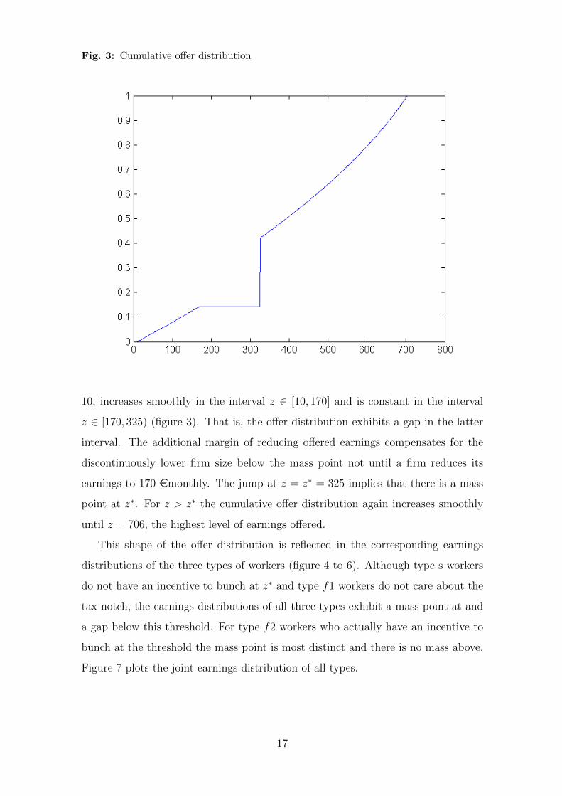
Fig. 3: Cumulative offer distribution
10, increases smoothly in the interval z ∈ [10, 170] and is constant in the interval
z ∈ [170, 325) (figure 3). That is, the offer distribution exhibits a gap in the latter
interval. The additional margin of reducing offered earnings compensates for the
discontinuously lower firm size below the mass point not until a firm reduces its
earnings to 170 emonthly. The jump at z = z∗ = 325 implies that there is a mass
point at z∗. For z > z∗ the cumulative offer distribution again increases smoothly
until z = 706, the highest level of earnings offered.
This shape of the offer distribution is reflected in the corresponding earnings
distributions of the three types of workers (figure 4 to 6). Although type s workers
do not have an incentive to bunch at z∗ and type f1 workers do not care about the
tax notch, the earnings distributions of all three types exhibit a mass point at and
a gap below this threshold. For type f2 workers who actually have an incentive to
bunch at the threshold the mass point is most distinct and there is no mass above.
Figure 7 plots the joint earnings distribution of all types.
17
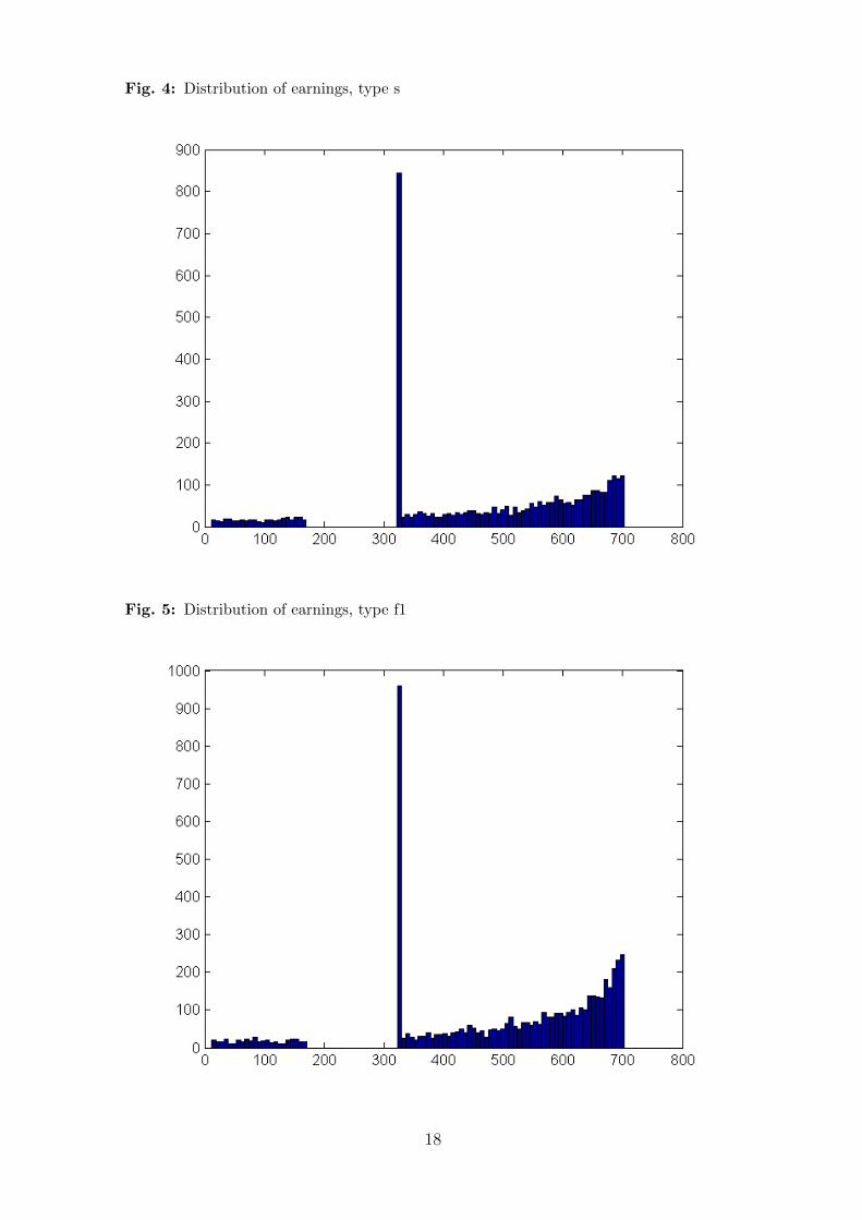
Fig. 4: Distribution of earnings, type s
Fig. 5: Distribution of earnings, type f1
18
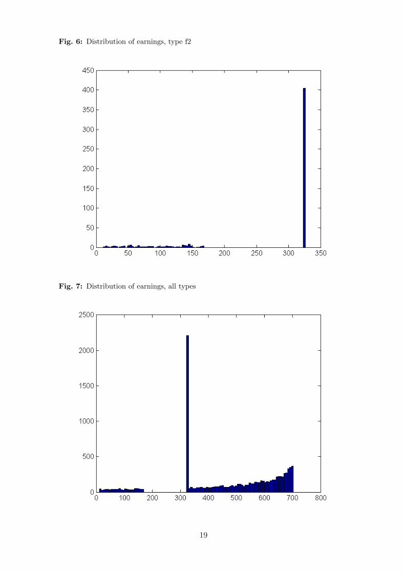
Fig. 6: Distribution of earnings, type f2
Fig. 7: Distribution of earnings, all types
19

5 Estimation
The estimation procedure we present here is based on the model with homogeneous
hours. Estimation of the model with heterogeneous hours is work in progress.
5.1 Notation
tub = elapsed unemployment duration
tuf = residual unemployment duration
dub = 1 if unemployment duration left-censored, otherwise 0
duf = 1 if unemployment duration right-censored, otherwise 0
teb = elapsed unemployment duration
tef = residual unemployment duration
deb = 1 if employment duration left-censored, otherwise 0
def = 1 if employment duration right-censored, otherwise 0
zu = earnings accepted by unemployed individuals
ze = earnings of employees in first period
j2j = 1 if job-to-job transition takes place
5.2 Likelihood contributions
An individual of type j who is initially unemployed and observed to start a job
paying zu has the following likelihood contribution (this follows Bontemps et al.
(1999)):
Lju(tub, tuf , zu) =(Dju)
2−dub−duf exp[−Dju(tub + tuf )]∗
f(zu)1−duf u
j
nj(10)
The first part of equation (10) pertains to the duration of the unem-
ployment spell. It is the joint density of elapsed and residual time in the
spell, f(tub, tuf ) = f(tuf |tub)f(tub) which both are exponentially distributed
with the exit rate Dju. Therefore, f(tuf |tub) = Dj
u1−duf exp[−Dj
utuf ] and
f(tub) = Dju1−dubexp[−Dj
utub]. The second part is the probability that the
accepted job has earnings zu. This part vanishes if the unemployment spell is
right-censored (i.e. duf = 1). The third part (uj) is the probability that an
20

unemployed individual is drawn in the initial state.
For an individual who is initially employed the likelihood contribution is
Lje(teb, tef , ze) =ej
njgj(ze)(D
je(z))2−deb−def exp[−Dj
e(z)(teb + tef )]∗
(δ1−j2jλ(1− F (ze))j2j)1−def (11)
The first part is the probability to be employed in a certain sector in the first
period with earnings we or q(we). The second part pertains to the duration of the
employment spell which is derived parallely to before. The last part is the probability
of a transition to unemployment (δ) or to a better job (λ(1− F (w))). It vanishes if
the employment spell is right-censored (i.e. def = 1).
The likelihood contributions differ between the worker types because of Dju,
Dje(.), u
j and ejk. While we observe if an individual is of type s or f , we cannot
distinguish between type f1 and f2 workers if observed wages are below the thresh-
old or not observed. If a type f worker is observed to have higher wages than the
threshold, she must be of type f1. For s = (u, e) and zs ≤ z∗6 the likelihood for
type f workers, therefore, is
Lfs (tsb, tsf , zs|zs ≤ z∗) =θnf
(1 + θ)nfLf2s (tsb, tsf , zs|zs ≤ z∗)+
nf
(1 + θ)nfLf1s (tsb, tsf , zs|zs ≤ z∗)
(12)
Note further that the presented likelihood contributions are only based on the
workers’ flow equations and only consider the initial state and the first transition.
5.3 Estimation procedure
For the moment the following description of the estimation process is restricted to
the case with homogeneous hours. Similar to Bontemps et al. (1999) we do not have
an analytical expression for F (.) which only depends on structural parameters.
Bontemps et al. (1999) apply a two-step procedure in which they first estimate
the cdf and pdf of the realized wage distribution (G and g) non-parametrically
6Conditioning on z ≤ z∗ mainly impacts the probability that an (un-)employed person is drawn
in the initial state.
21

by kernel density estimators. Using these estimates and equations (4) and (6),
the likelihood contributions can be expressed in terms of G, g and the model
parameters. Once the transition parameters are estimated from workers’ mobility
patterns, these can be used to transform the observed distribution G(.) to the
offer distribution F (.) which is the object about which theory provides us with
predictions concerning the likelihood.
As this strategy only exploits equations with respect to workers’ behaviour, the
offer distribution is basically treated as exogenous. Firms’ behaviour (described by
the equal profit conditions above) which lead to the endogenous offer distribution
is not exploited.
However, in our setting, besides the transition parameters, we need to identify
θ, the unobserved fraction of type f workers who accept jobs with z > z∗ (type
f1) or those who don’t (type f2). Intuitively it makes sense that the size of the
mass point at the earnings threshold will be informative of the amount of individ-
uals who are subject to the incentives generated by the threshold, i.e. θ. Thus it
makes sense to use the theoretical restrictions on the wage distribution in estimation.
Note that - in our simple model at least - we can identify θ without the earnings
distribution akin to Bontemps et al. (1999) based solely on workers’ behaviour.
Without worker heterogeneity7, i.e. every job offer is accepted by type s and f1
individuals, the only driver for a correlation between unemployment duration and
accepted wage are the type f2 workers. The reason is that the latter do not accept
jobs with w > w∗ which is why the probability of a match in one period is λfF (w∗).
For other workers this probability is simply λf or λs, respectively. The extent of
correlation between the unemployment duration and the wage, thus, is informative
about θ.
7Worker heterogeneity would also introduces such a correlation (albeit in the opposite direc-
tion). If the distribution of reservation wages is assumed to be identical for the different groups,
identification is enhanced by comparing the durations above and below the threshold and between
type s and type f workers. Further, while the reservation wage distribution is arguably smooth
around the threshold, durations might change discontinuously.
22

Although not necessary in our simple model, we think that making use of the
restrictions put on the wage distribution (by the equal profit conditions) will create
a more robust estimate of θ. We exploit that the relative size of the mass point
in the offer distribution at the threshold contains information about the fraction of
type f2 workers (and, thus, θ). By contrast to the two-step process proposed by
Bontemps et al. (1999) we, therefore, replace g(.) in the likelihood expressions by a
function of F or f and solve in every iteration the system of equal profit conditions
which defines the offer distribution F (.) subject to the structural parameters.
6 Data
The Sample of Integrated Labour Market Biographies (SIAB) is a representative
two percent sample of all individuals for whom an employer’s report to the social
security system exists8. For the present analysis, its specific characteristics makes
the SIAB the most suited data set. First, exact total gross earnings of a period
of an employment report are observed9. This information is very accurate due to
the administrative character of the data. Second, with approximately 1.6 million
sampled employees, the sample size is comparatively large and, therefore, includes
a substantial amount of individuals holding second jobs. It does not include civil
servants and self-employed. Third, the SIAB consists of complete employment
biographies of the sampled individuals. We can, therefore, differentiate between
first and second employments and observe, for example, the exact day a second
employment starts as well as earnings changes over time. Fourth, we observe several
characteristics important for labour market outcomes. On individual level this
particularly includes age, sex, occupation and education. Further, experience and
tenure can be derived. On firm level, industry sector, size and wage structure are
especially noteworthy. Furthermore, a regional unemployment rate can be matched
based on the district of workplace.
The SIAB has three main limitations. First, minijobs are only included as of
the middle of 1999. Second, working time is only differentiated between full- and
8See Dorner et al. (2011) for a detailed description of the data.9A period lasts at most until the end of the calender year. Gross earnings are capped at the
earnings cap of pension insurance which is not problematic here as we focus on low-paid jobs.
23

part-time employment. The amount of hours worked is not exactly observed. Hours
information only exists in three broad categories. Third, we do not observe the
household context like marriage status, the income of a potential spouse or other
income sources which precludes the calculation of the exact income tax rates.
We restrict the sample to full-time employees between 18 and 62 years and
exclude old-age pensioners. Spells with daily gross earnings below one Euro as
well as one-time payments are excluded. If an individual has two parallel full-time
employments the employment with less earnings is excluded. As the education
variable is not necessary for the administrative process, the quality is not as good
as for most other variables (Dorner et al., 2011). Therefore, it is improved by the
first imputation procedure proposed by Fitzenberger et al. (2006) which is shown to
perform best (Wichert and Wilke, 2012).
Second jobs are identified by the following procedure. Parallel spells10 are ranked
by earnings with highest earnings as first rank. Yearly second job earnings, then,
are the sum of earnings of all employments of second rank. That is, yearly second
job earnings are not necessarily generated by a single employment relation because
its rank can vary. Therefore, the sample is (so far) restricted to employees holding
their first jobs the entire year. We, further, exclude employees if first and second
jobs switch.
6.1 Descriptive Evidence
The response of first job earnings to the notch in the budget set is dramatic
(Figure 8). There is a huge peak at the threshold for minijobs implying that
individuals adjust their labour supply to their individual incentives. Figure 9 plots
the empirical density of daily second job earnings for the year 2002 given yearly
first job earnings exceed 5000 e. The density features a clear peak at the minijob
threshold and hardly any mass beyond. As in 2002 second jobs were not eligible for
the favourable tax treatment of minijobs (they had to be taxed jointly with first
job earnings), this is strong evidence that other workers’ preferences matter as well.
Firms seem to cater offered wage hours packages to employees looking for minijobs
10Note that in the SIAB data set only completely parallel spells exist. If two spells partly
overlaps, original spells are split.
24

Fig. 8: Distribution of first job earnings in 2002
as first jobs.
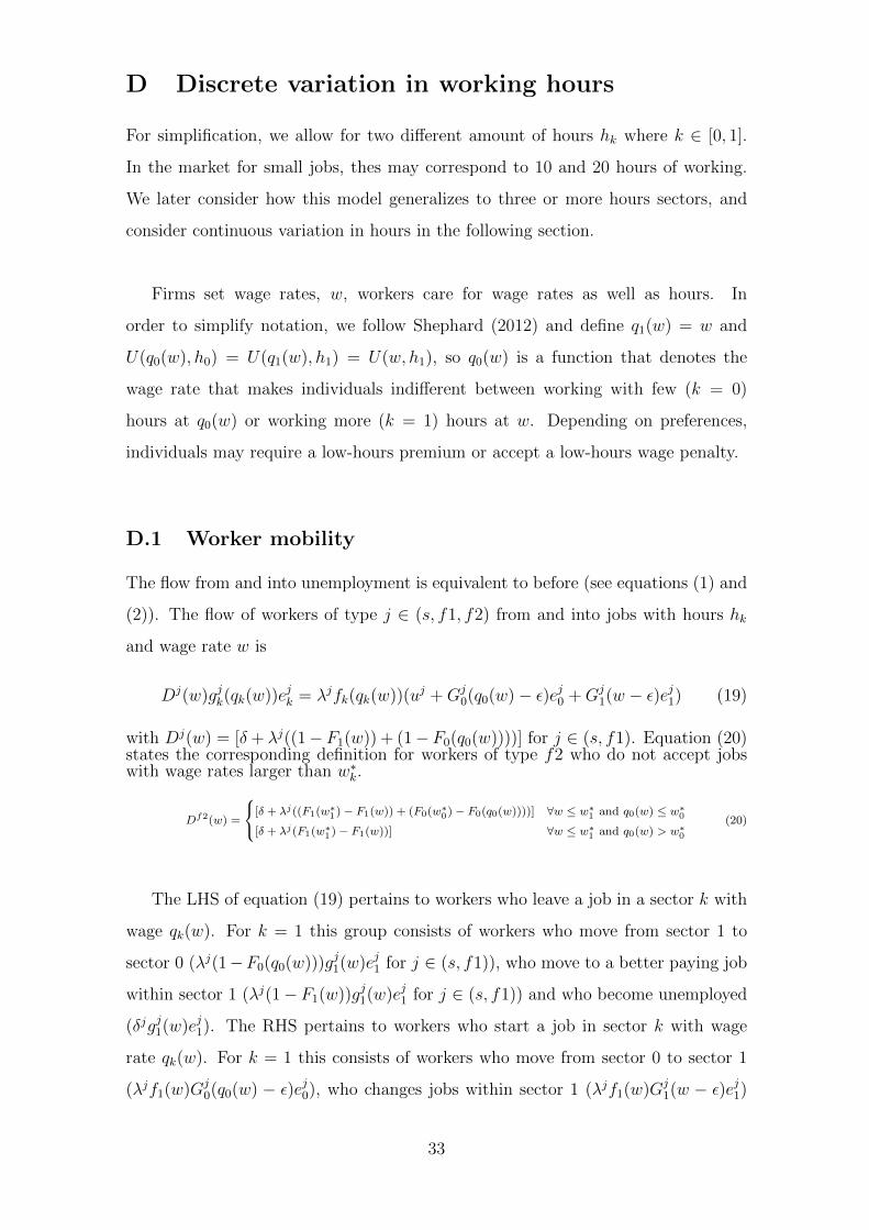
Figures 8 and 9 contain the same graphs for 2005, two years after the reform
which, among others, increased the threshold to 400 e per month and extended the
coverage to second jobs. The red lines mark the old threshold. For both, first and
second jobs, the peak moved to the new threshold. While for first jobs this seems
to be the only noteworthy change, the amount of second jobs increased tremendously.
As our data differentiates between minijobs and employments subject to SSC we
can actually test whether misclassifying first as second jobs can be the reason for
the discontinuity in the density of the latter. Table 1 shows that this is not the case.
Almost all first (second) jobs with daily earnings below the threshold are classified
as minijobs (employment subject to SSC).
Table 2 shows the different sectors in which minijobs are found - according to
whether these are first jobs (first column), second jobs (second column) or first jobs
of employees holding second jobs. The distributions are consistent with the idea
25
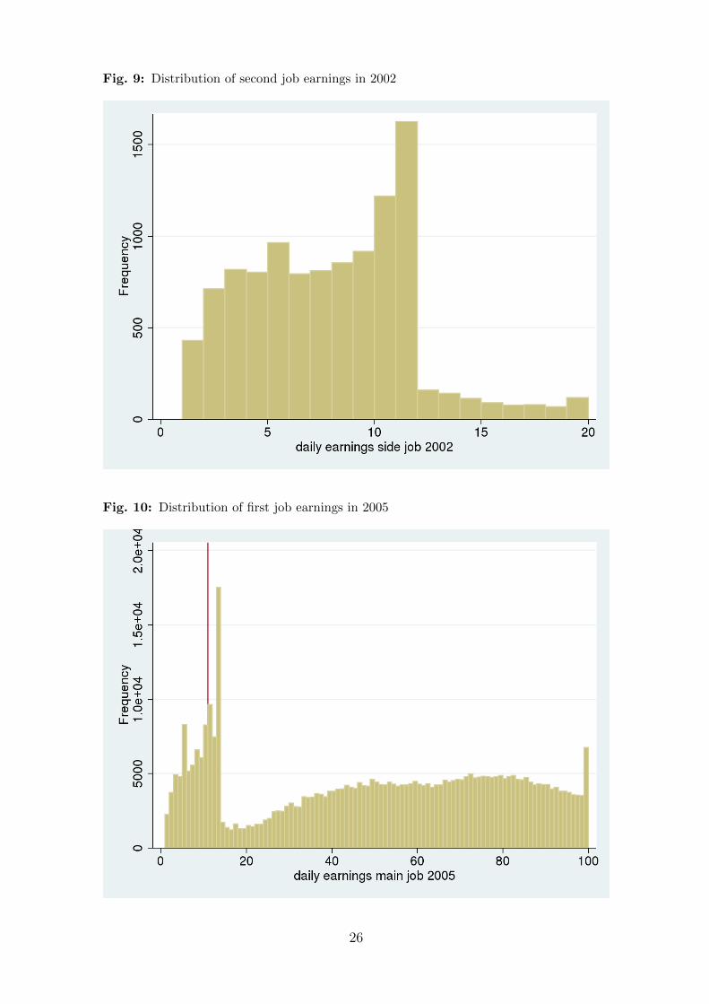
Fig. 9: Distribution of second job earnings in 2002
Fig. 10: Distribution of first job earnings in 2005
26
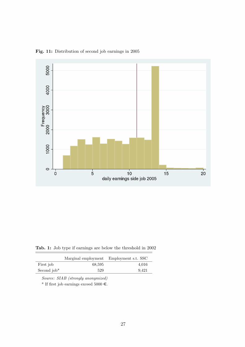
Fig. 11: Distribution of second job earnings in 2005
Tab. 1: Job type if earnings are below the threshold in 2002
Marginal employment Employment s.t. SSC
First job 68,595 4,016
Second job* 529 9,421
Source: SIAB (strongly anonymized)
* If first job earnings exceed 5000 e.
27

that offers for first and second jobs are drawn from the same wage offer distribution:
The main sectors are economic and household services as well as cleaning. The only
striking difference between minijobs as first and as second jobs is the particularly
high incidence of retail industry in the former group. The sector distribution of all
first jobs (of second job holders) is much more different. Only 20 % of employees
with second jobs work in the same sector in both jobs. With respect to occupations
this is true for 23 %.11 32 % work in both jobs in either the same sector or the same
occupation. That is, it seems that the lion’s share of second jobs are not advisory
activities of professors or the like.
Tab. 2: Distribution of sectors, 2000-2002
Marginal Employment 1st jobs of
Sector 1st job 2nd job 2nd job hold.
1 Agriculture, energy, mining 1,591 2 344 1 519 2
2 Primary production, prod. of goods 1,396 1 454 1 1,536 5
3 Facture of structural metal products 2,081 2 834 2 2,445 7
4 Steel deformation, vehicle constr. 2,465 2 720 2 2,340 7
5 Consumer goods industry 3,283 3 819 2 1,675 5
6 Food and luxury food industry 3,783 4 629 2 892 3
7 Main construction industry 1,244 1 449 1 721 2
8 Finishing trade 1,933 2 510 1 615 2
9 Wholesale trade 5,732 6 2,066 6 1,685 5
10 Retail industry 17,923 18 2,540 7 2,524 8
11 Transport and communication 3,246 3 2,136 6 1,806 5
12 Economic services 21,549 22 10,907 30 4,564 14
13 Household services 12,209 12 4,990 14 1,483 4
14 Education, social and health-care 7,022 7 2,993 8 4,952 15
15 (Street)Cleaning, organisations 12,395 12 4,443 12 2,664 8
16 Public admin., social security 1,941 2 1,215 3 2,717 8
Source: SIAB (strongly anonymized)
Table 3 compares the difference between desired and actual (or contracted) hours
of work for employees with and without a second job12. The fraction of underem-
ployed workers is larger for holders of second jobs, especially if desired are compared
to contractual instead of actual hours of work. This implies that second jobs are used
to compensate for potential hours restrictions in the first job. However, most holders
of second jobs do not state that they are underemployed. Although the robustness
11These numbers depend on the aggregation level. Here, sectors are aggregated to 17 and
occupations to 120 groups.12This information is taken from the German Socio Economic Panel which cannot be matched
(on individual level) to our main data set.
28

of such survey data is arguably not very high, this suggests that other motivations
for second jobs - like for example the heterogeneity of jobs - are important as well
(which is for example also found by Smith Conway and Kimmel (1998)).
Tab. 3: Differences between actual and desired hours of work, 2002
Actual hours Contracted hours
With second job Without second job With second job Without second job
N % N % N % N %
Underemployed 45 11 520 6 84 20 1035 12
No difference 243 58 5484 66 292 70 6420 78
Overemployed 132 31 2266 27 44 10 815 10
Notes: No difference is defined with a tolerance of +-5
Source: SOEP wave 2002
Tab. 4: Socio-demographic characteristics in 2000-2002
With second job Without second job
female .56 .47
age 40.74 41.27
German .86 .92
East German .07 .18
Education
Intermediate .22 .12
Voc. training .62 .65
Grammar .04 .05
University .05 .09
Source: SIAB (strongly anonymized)
At first glance, the mean hourly wage13 is much larger in the second (22.5 e)
than the first job (15.5 e). For the median wage rate, however, the opposite is true
(12.5 vs. 14 e). Further, restricting second jobs to those with more than 5 work
days a month also decreases the hourly wage (mean=14.8 e).
7 Conclusion
We present a job search model in which firms tailor their offers to the preferences of
the most likely job seeking candidates. As a result, workers’ labour supply depends
on other workers’ preferences. Given that labour supply in the market for marginal
13This information is taken from the German Socio Economic Panel which cannot be matched
(on individual level) to our main data set.
29

employment in Germany is strongly influenced by non-linearities in the tax schedule
induced by special treatment of marginal employment below an earnings threshold,
so-called minijobs, we can identify the importance of this channel by considering the
labour supply of individuals who are not affected by specific non-linearities. The
effect of aggregate preferences of individual labour supply will mean that standard
analyses of labour market policy are not reliable, since workers’ choice over hours is
not independent of other workers. This provides a rationale for differences between
micro- and macro labour supply elasticities. Whilst this possibility has already been
voiced in the literature, we are the first to present an estimable structural model.
Estimation is work in progress. The model will allow us to perform counterfactual
policy analyses, including new estimates of tax incidence.
A Sketch of Proof of Proposition (I)
Proposition (I) If we observe offers above z∗, there must be a mass point of job
offers at z∗. The wage offer distribution above z∗ is continuous up to some z.
Above-threshold wages imply mass-point
Assume there exists no mass point (i.e. f(z∗) = 0), the offer distribution for z < z∗
is then continuous and profits at the mass point are
π(z∗) = (p− z
∗)
nsκs
(1 + κs(1 − F (z∗)))2+
nfκf
(1 + κf (1 − F (z∗)))2+ θn
fκf. (13)
The profit of a firm offering jobs with earnings slightly above the threshold (for
ε→ 0) is:
π(z∗+ ε) = (p− (z
∗+ ε))
nsκs
(1 + κs(1 − F (z∗ + ε)))(1 + κs(1 − F (z∗ − ε + ε)))+
nfκf
(1 + κf (1 − F (z∗ + ε)))(1 + κf (1 − F (z∗ − ε + ε)))
= (p− z∗)
nsκs
(1 + κs(1 − F (z∗)))2+
nfκf
(1 + κf (1 − F (z∗)))2(14)
Comparing equations (13) and (14) and assuming f(z∗) = 0, it is obvious that
π(z∗ + ε) < π(z∗) implying that there is a gap to the right of the threshold. Is
there an earnings level z′ > z∗ + ε where the equal profit condition holds again?
Equation (15) makes use of F (z′) = F (z∗) which holds if there is a gap in the
interval z ∈ (z∗, z′).
30

π(z′) = (p− z
′)
nsκs
(1 + κs(1 − F (z′)))(1 + κs(1 − F (z′ − ε)))+
nfκf
(1 + κf (1 − F (z′)))(1 + κf (1 − F (z′ − ε)))
= (p− (z′))
nsκs
(1 + κs(1 − F (z∗)))2+
nfκf
(1 + κf (1 − F (z∗)))2(15)
As (p − z′) < (p − z∗) it holds that π(z′) < π(z∗) implying that no job with
earnings z > z∗ will be offered if there is no mass point at z∗.
Allowing for the existence of a mass point at z∗, ∂π(z∗)∂f(z∗)
< 0 and ∂π(z∗+ε)∂f(z∗)
= 0
imply that there might be a value for f(z∗) for which the equal profit condition
between z∗ and z∗ + ε holds (π(z∗ + ε) = π(z∗)).
The equilibrium offer distribution for the interval z′ ∈ [z∗+ ε, z] is, then, contin-
uous and determined by π(z′) = π(z∗ + ε).
B Sketch of proof of Proposition (2)
Proposition (II) If there is a mass point at z∗, there will be a gap in the offer
distribution just below the threshold.
We need to show that a mass point in the wage offer distribution is only
consistent with equal profits if there is a gap in the wage offering distribution. We
compare profits π(z∗) with profits π(z∗ − ε).
The profit of a firm offering jobs with earnings at the threshold is
π(z∗) = (p− z
∗)l(z∗)
= (p− z∗)(
nsκs
(1 + κs(1 − F (z∗)))(1 + κs(1 − F (z∗ − ε)))+
nfκf
(1 + κf (1 − F (z∗)))(1 + κf (1 − F (z∗ − ε)))+
θnfκf
(1 + κf (F (z∗) − F (z∗)))(1 + κf (F (z∗) − F (z∗ − ε))))
= (p− z∗)(
nsκs
(1 + κs(1 − F (z∗)))(1 + κs(1 − F (z∗) + f(z∗)))+
nfκf
(1 + κf (1 − F (z∗)))(1 + κf (1 − F (z∗) + f(z∗)))+
θnfκf
(1 + κf f(z∗)))(16)
Given proposition (I), the data implies that there is a mass point at z = z∗ (i.e.
that f(z∗) > 0). Assuming, thus, that f(z∗) > 0 and z < z∗, the profit slightly
below the threshold can be given by (for ε→ 0):
31

π(z∗ − ε) = (p− (z
∗ − ε))(nsκs
(1 + κs(1 − F (z∗ − ε)))(1 + κs(1 − F (z∗ − 2ε)))+
nfκf
(1 + κf (1 − F (z∗ − ε)))(1 + κf (1 − F (z∗ − 2ε)))+
θnfκf
(1 + κf (F (z∗) − F (z∗ − ε)))(1 + κf (F (z∗) − F (z∗ − 2ε))))
= (p− z∗)(
nsκs
(1 + κs(1 − F (z∗ − ε)))2+
nfκf
(1 + κf (1 − F (z∗ − ε)))2+
θnfκf
(1 + κf (f(z∗)))2)
= (p− z∗)(
nsκs
(1 + κs(1 − F (z∗) + f(z∗)))2+
nfκf
(1 + κf (1 − F (z∗) + f(z∗)))2+
θnfκf
(1 + κf (f(z∗)))2)
Given the assumption that f(z∗) > 0, it holds that (1 +κj(1−F (z∗) +f(z∗))) >
(1 + κj(1− F (z∗))) and (1 + κf (f(z∗))) > 1. Therefore, π(z∗) > π(z∗ − ε) implying
that there will be a gap to the left of the threshold.
C Sketch of proof of proposition (III)
Proposition (III) There may or may not exist wage offers offers below the
threshold z∗ in equilibrium. The wage offer distribution will then be continuous
between z ∈ [z, z′′]for z′′ < z∗.
Define the highest wage offer below the threshold as z′′, such that F (z′′) =F (z∗ − ε). Note that since there is a gap left of the threshold, if in equilibrium az′′-offer exists, it may be significantly below z∗. In equilibrium any z′′-offer mustmake the same amount of profits as the threshold wage offer z∗.
π(z′′) = (p− z
′′)
nsκs
(1 + κs(1 − F (z′′)))(1 + κs(1 − F (z′′ − ε)))+
nfκf
(1 + κf (1 − F (z′′)))(1 + κf (1 − F (z′′ − ε)))+
θnfκf
(1 + κf (F (z∗) − F (z′′)))(1 + κf (F (z∗) − F (z′′ − ε)))
= (p− z′′)
nsκs
(1 + κs(1 − F (z∗) + f(z∗)))2+
nfκf
(1 + κf (1 − F (z∗) + f(z∗)))2+
θnfκf
(1 + κf (f(z∗)))2(17)
Comparing equations (16) and (17) illustrates that π(z′′) = π(z∗) can hold as
π(z′′) increases with decreasing z′′. That is, there might be a certain size of the gap
where π(z′′) = π(z∗) holds.
Using that F (z) = 0, we now determine the lowest wage offer z that will be
made (if there are wage offers below z∗).
π(z) = (p− z)nsκs
(1 + κs(1 − F (z)))(1 + κs(1 − F (z − ε)))+
nfκf
(1 + κf (1 − F (z)))(1 + κf (1 − F (z − ε)))+
θnfκf
(1 + κf (F (z∗) − F (z)))(1 + κf (F (z∗) − F (z − ε)))
= (p− z)nsκs
(1 + κs)2+
nfκf
(1 + κf )2+
θnfκf
(1 + κf (F (z∗)))2(18)
If z′′ < z∗ exists and z < z′′ there will then be a continuity of wage offers be-
tween these two values, generating equal profits with the standard trade-off between
margins and firm-size.
32
D Discrete variation in working hours
For simplification, we allow for two different amount of hours hk where k ∈ [0, 1].
In the market for small jobs, thes may correspond to 10 and 20 hours of working.
We later consider how this model generalizes to three or more hours sectors, and
consider continuous variation in hours in the following section.
Firms set wage rates, w, workers care for wage rates as well as hours. In
order to simplify notation, we follow Shephard (2012) and define q1(w) = w and
U(q0(w), h0) = U(q1(w), h1) = U(w, h1), so q0(w) is a function that denotes the
wage rate that makes individuals indifferent between working with few (k = 0)
hours at q0(w) or working more (k = 1) hours at w. Depending on preferences,
individuals may require a low-hours premium or accept a low-hours wage penalty.
D.1 Worker mobility
The flow from and into unemployment is equivalent to before (see equations (1) and
(2)). The flow of workers of type j ∈ (s, f1, f2) from and into jobs with hours hk
and wage rate w is
Dj(w)gjk(qk(w))ejk = λjfk(qk(w))(uj +Gj0(q0(w)− ε)ej0 +Gj
1(w − ε)ej1) (19)
with Dj(w) = [δ + λj((1− F1(w)) + (1− F0(q0(w))))] for j ∈ (s, f1). Equation (20)states the corresponding definition for workers of type f2 who do not accept jobswith wage rates larger than w∗k.
Df2(w) =
[δ + λj((F1(w∗1)− F1(w)) + (F0(w∗
0)− F0(q0(w))))] ∀w ≤ w∗1 and q0(w) ≤ w∗
0
[δ + λj(F1(w∗1)− F1(w))] ∀w ≤ w∗
1 and q0(w) > w∗0
(20)
The LHS of equation (19) pertains to workers who leave a job in a sector k with
wage qk(w). For k = 1 this group consists of workers who move from sector 1 to
sector 0 (λj(1−F0(q0(w)))gj1(w)ej1 for j ∈ (s, f1)), who move to a better paying job
within sector 1 (λj(1− F1(w))gj1(w)ej1 for j ∈ (s, f1)) and who become unemployed
(δjgj1(w)ej1). The RHS pertains to workers who start a job in sector k with wage
rate qk(w). For k = 1 this consists of workers who move from sector 0 to sector 1
(λjf1(w)Gj0(q0(w) − ε)ej0), who changes jobs within sector 1 (λjf1(w)Gj
1(w − ε)ej1)
33

and who come from unemployment (λjf1(w)). The overall flow (i.e. both sectors)
between jobs with wage rate of no greater than w and unemployment is:
(Gj0(q0(w))ej0 +Gj
1(w)ej1)Dj(w) = λjujF0(q0(w)) + λjujF1(w)
= λjuj + λjuj − λjuj(1− F0(q0(w)))− λjuj(1− F1(w)) (21)
Using equation (1) gives
Gj0(q0(w))ej0 +Gj
1(w)ej1 =δnj − ujDj(w)
Dj(w)(22)
By combining equations (19) and (22) we obtain
gjk(qk(w))ejk =λjfk(qk(w))(uj + δnj−uj(Dj(w−ε))
Dj(w−ε)
Dj(w)(23)
D.1.1 Firm size
The amount of workers of type j in steady-state employed at a firm in sector k which
offers wage rate qk(w) is
ljk(qk(w)) =gjk(qk(w))ejkfk(qk(w))
=λjδnj
Dj(w)Dj(w − ε)(24)
The steady state firm size is then
lk(qk(w)) = lsk(qk(w)) + lf1k (qk(w)) + lf2k (qk(w))
=
λsδns
Ds(w)Ds(w−ε) + λf δnf1
Df1(w)Df1(w−ε) + λf δnf2
Df2(w)Df2(w−ε) ∀w ≤ w∗
λsδns
Ds(w)Ds(w−ε) + λf δnf1
Df1(w)Df1(w−ε) ∀w > w∗(25)
Following the standard arguments of profit equalization, we find the following
(the reasoning is parallel to the case without hours variation):
Proposition (A1) There can be (at most one) mass point in the wage offer
distribution at the threshold in each sector, i.e. at wages w∗k ≡ z∗
hk.
Sketch of Proof : The following argument closely mirrors the argument in the
case of homogeneous hours. We compare profits at the threshold value with profits
above. We find that if there are offers above, there must be a mass point at the
34

threshold.
The profit of a sector k firm offering wage rate qk(w) can be expressed asπk(qk(w)) = (phk − qk(w)hk)lk(qk(w)). We first state the profits of a type-1-firm,assuming that q0(w
∗1) ≤ w∗0.
πk(w∗1 ) =
λsδns
Ds(w∗k)Ds(w∗
k− ε)
+λf δnf1
Df1(w∗k)Df1(w∗
k− ε)
+λf δnf2
Df2(w∗k)Df2(w∗
k− ε)
=λsδns
[δ + λs((1 − F1(w∗1 )) + (1 − F0(q0(w
∗1 ))))][δ + λs((1 − F1(w
∗1 − ε)) + (1 − F0(q0(w
∗1 ) − ε)))]
+
+λf δnf1
[δ + λf ((1 − F1(w∗1 )) + (1 − F0(q0(w
∗1 ))))][δ + λf ((1 − F1(w
∗1 − ε)) + (1 − F0(q0(w
∗1 ) − ε)))]
+
+λf δnf2
[δ + λj(F0(w∗0 ) − F0(q0(w
∗1 )))][δ + λj(f1(w
∗1 ) + (F0(w
∗0 ) − F0(q0(w
∗1 ) − ε)))]
(26)
Evaluated slightly above the threshold, profits are
πk(w∗1 + ε) =
λsδns
Ds(w∗k
+ ε)Ds(w∗k)+
λf δnf1
Df1(w∗k
+ ε)Df1(w∗k)
=λsδns
[δ + λs((1 − F1(w∗1 + ε)) + (1 − F0(q0(w
∗1 + ε))))][δ + λs((1 − F1(w
∗1 )) + (1 − F0(q0(w
∗1 ))))]
+
+λf δnf1
[δ + λf ((1 − F1(w∗1 + ε)) + (1 − F0(q0(w
∗1 + ε))))][δ + λf ((1 − F1(w
∗1 )) + (1 − F0(q0(w
∗1 ))))]
(27)
Equations (26) and (27) shows that the equal profit condition can only hold if
there is a mass point in the offer distribution of sector 1 at w∗1. By symmetry, note
that the same argument can be made with respect to a type-0 firm. However, if
the utility of a threshold offer lies in the “gap area” due to a threshold in another
sector, it may be the case that there is no mass point in that sector. This explains
the restriction “at most one” in Proposition (IV) and completes this sketch of a
proof.
We now consider the influence of thresholds in other hours sectors on the wage
distribution. Consider a firm of type-1, i.e. seeking a worker to work for h1 hours.
The impact of a potential mass point in the offer distribution of sector 0 at w∗0
depends on the relation between w∗1, q0(w∗1) and w∗0.
Proposition (A2) There will be no wage offers at wage levels (and in a certain
interval below this level) that offer the same utility as is available at threshold wages
w∗j 6= k in other sectors.
The intuition for Proposition (A2) is the following: It is a dominated strategy to
offering a wage rate that is equal in utility to an offer made by several other firms.
A slightly higher offer will attract all workers from these firms at only marginal
35

cost. By Proposition (IV), wage offers at earnings thresholds generate mass points
in the wage offer distributions. Thus for example a type-1 firm will offer a wage
rate slightly larger than w1 (where U(w1, h1) = U(w∗0, h0).) in order to additionally
attracts workers from this positive mass of sector 0 firms. This implies that there
must be a gap in the wage offer distribution at w1. How much below this utility
value an offer can be sustained in equilibrium will depend on the parameters of the
model in an analogous way to the potential existence of offers below the threshold
offer in the homogeneous case.
Sketch of proof of Proposition (A2)Let w1 denote the wage rate which satisfies U(w1, h1) = U(w∗0, h0). If w1 > w∗1 theprofits of a sector 1 firm offering wage rate w1 and slightly above are:
πk(w1) =λsδns
Ds(wk)Ds(wk − ε)
+λf δnf1
Df1(wk)Df1(wk − ε)
+λf δnf2
Df2(wk)Df2(wk − ε)
=λsδns
[δ + λs((1 − F1(w1)) + (1 − F0(w∗0 )))][δ + λs((1 − F1(w1 − ε)) + (1 − F0(w
∗0 − ε)))]
+
+λf δnf1
[δ + λf ((1 − F1(w1)) + (1 − F0(w∗0 )))][δ + λf ((1 − F1(w1 − ε)) + (1 − F0(w
∗0 − ε)))]
+
+λf δnf2
[δ + λj((F1(w∗1 ) − F1(w1)) + (F0(w
∗0 ) − F1(w
∗0 ))))][δ + λj((F1(w
∗1 ) − F1(w1 − ε)) + (F0(w
∗0 ) − F1(w
∗0 − ε)))]
=λsδns
[δ + λs((1 − F1(w1)) + (1 − F0(w∗0 )))][δ + λs((1 − F1(w1)) + (1 − F0(w
∗0 ) + f0(w
∗0 ))))]
+
+λf δnf1
[δ + λf ((1 − F1(w1)) + (1 − F0(w∗0 )))][δ + λf ((1 − F1(w1)) + (1 − F0(w
∗0 ) + f0(w
∗0 )))]
+
+λf δnf2
[δ + λj((F1(w∗1 ) − F1(w1)))][δ + λj((F1(w
∗1 ) − F1(w1)) + f0(w
∗0 ))]
(28)
πk(w1 − ε) =λsδns
Ds(wk − ε)Ds(wk − 2ε)+
λf δnf1
Df1(wk − ε)Df1(wk − 2ε)+
λf δnf2
Df2(wk − ε)Df2(wk − 2ε)
=λsδns
[δ + λs((1 − F1(w1 − ε)) + (1 − F0(w∗0 − ε)))][δ + λs((1 − F1(w1 − 2ε)) + (1 − F0(w
∗0 − 2ε)))]
+
+λf δnf1
[δ + λf ((1 − F1(w1 − ε)) + (1 − F0(w∗0 − ε)))][δ + λf ((1 − F1(w1 − 2ε)) + (1 − F0(w
∗0 − 2ε)))]
+
+λf δnf2
[δ + λj((F1(w∗1 ) − F1(w1 − ε)) + (F0(w
∗0 ) − F1(w
∗0 − ε)))][δ + λj((F1(w
∗1 ) − F1(w1 − 2ε)) + (F0(w
∗0 ) − F1(w
∗0 − 2ε)))]
=λsδns
[δ + λs((1 − F1(w1)) + (1 − F0(w∗0 ) + f0(w
∗0 )))]
2+
+λf δnf1
[δ + λf ((1 − F1(w1)) + (1 − F0(w∗0 ) + f0(w
∗0 )))]
2+
+λf δnf2
[δ + λj((F1(w∗1 ) − F1(w1)) + f0(w
∗0 ))]
2(29)
36

πk(w1 + ε) =λsδns
Ds(wk + ε)Ds(wk)+
λf δnf1
Df1(wk + ε)Df1(wk)+
λf δnf2
Df2(wk + ε)Df2(wk)
=λsδns
[δ + λs((1 − F1(w1 + ε)) + (1 − F0(w∗0 + ε)))][δ + λs((1 − F1(w1)) + (1 − F0(w
∗0 )))]
+
+λf δnf1
[δ + λf ((1 − F1(w1 + ε)) + (1 − F0(w∗0 + ε)))][δ + λf ((1 − F1(w1)) + (1 − F0(w
∗0 )))]
+
+λf δnf2
[δ + λj((F1(w∗1 ) − F1(w1 + ε)))][δ + λj((F1(w
∗1 ) − F1(w1)))]
(30)
=λsδns
[δ + λs((1 − F1(w1)) + (1 − F0(w∗0 )))]
2+
+λf δnf1
[δ + λf ((1 − F1(w1)) + (1 − F0(w∗0 )))]
2+
+λf δnf2
[δ + λj((F1(w∗1 ) − F1(w1)))]2
(31)
As f0(w∗0) > 0 and ε→ 0, it holds that πk(w1 − ε) < πk(w1) < πk(w1 + ε). This
implies that there will be no wage offers of value w1.
As (ph− wh) increases with decreasing w, there might be a wage rate w′ where
it holds that πk(w′) = πk(w1 + ε).
This implies f1(.) exhibit a gap in the interval (w’,w1]. If w1 < w∗1, the terms
of equations (28) and (30) referring to workers of type f2 drop out. Although this
might reduce the extent of the gap, πk(w1) < πk(w1 + ε) still holds. If w1 = w∗1
the necessary size of the mass point at w∗1 to balance the loss of type f2 workers
decreases (in comparison to w1 6= w∗1). How large the gap is, i.e. whether any offers
will be made below w1 will depend on the economic environment captured by the
parameters of the model.
E Derivation of firm-size
The following derivation uses equations (4), (7) and (1).
37

lj(z) =
F (z)1+κj(1−F (z))
− F (z−ε)1+κj(1−F (z−ε))
F (z)− F (z − ε)(nj − uj)
=
F (z)(1+κj(1−F (z−ε)))−F (z−ε)(1+κj(1−F (z)))(1+κj(1−F (z)))(1+κj(1−F (z−ε)))
F (z)− F (z − ε)(nj − uj)
=
F (z)+F (z)κj−F (z)κjF (z−ε)−(F (z−ε)+F (z−ε)κj−F (z−ε)κjF (z))(1+κj(1−F (z)))(1+κj(1−F (z−ε)))
F (z)− F (z − ε)(nj − uj)
=
F (z)+F (z)κj−(F (z−ε)+F (z−ε)κj)(1+κj(1−F (z)))(1+κj(1−F (z−ε)))
F (z)− F (z − ε)(nj − uj)
=
(F (z)−F (z−ε))(1+κj)(1+κj(1−F (z)))(1+κj(1−F (z−ε)))
F (z)− F (z − ε)(nj − uj)
=(1 + κj)
(1 + κj(1− F (z)))(1 + κj(1− F (z − ε)))(nj − uj)
=(1 + κj)
(1 + κj(1− F (z)))(1 + κj(1− F (z − ε)))njκ
1 + κj
=njκ
(1 + κj(1− F (z)))(1 + κj(1− F (z − ε)))
For type f2 workers, we use equations (6), (7) and (2). For earnings z < z∗ we
get
lf2(z) =
F (z)(1+κf (F (z∗)−F (z)))F (z∗)
− F (z−ε)(1+κf (F (z∗)−F (z−ε)))F (z∗)
F (z)− F (z − ε)(θnf − uf2)
=
F (z)((1+κf (F (z∗)−F (z−ε)))F (z∗))−F (z−ε)((1+κf (F (z∗)−F (z)))F (z∗))((1+κf (F (z∗)−F (z)))F (z∗))((1+κf (F (z∗)−F (z−ε)))F (z∗))
F (z)− F (z − ε)(θnf − uf2)
=
(F (z)+F (z)κfF (z∗)−F (z)κfF (z−ε)−(F (z−ε)+F (z−ε)κfF (z∗)−F (z−ε)κfF (z)))F (z∗)F (z∗)2(1+κf (F (z∗)−F (z)))(1+κf (F (z∗)−F (z−ε)))
F (z)− F (z − ε)(θnf − uf2)
=
(F (z)+F (z)κfF (z∗)−(F (z−ε)+F (z−ε)κfF (z∗)))F (z∗)(1+κf (F (z∗)−F (z)))(1+κf (F (z∗)−F (z−ε)))
F (z)− F (z − ε)(θnf − uf2)
=
(F (z)−F (z−ε))(1+κfF (z∗))F (z∗)(1+κf (F (z∗)−F (z)))(1+κf (F (z∗)−F (z−ε)))
F (z)− F (z − ε)(θnf − uf2)
=(1 + κfF (z∗))
F (z∗)(1 + κf (F (z∗)− F (z)))(1 + κf (F (z∗)− F (z − ε)))(θnf − uf2)
=(1 + κfF (z∗))
F (z∗)(1 + κf (F (z∗)− F (z)))(1 + κf (F (z∗)− F (z − ε)))θnfκfF (z∗)
1 + κfF (z∗)
=θnfκf
(1 + κf (F (z∗)− F (z)))(1 + κf (F (z∗)− F (z − ε)))
The total firm size, is then the sum of the amount of workers of each type, which
gives expression (8).
38

F Derivation of firm profits
The profit of a firm offering jobs with earnings at the threshold is
π(z∗) = (p− z
∗)l(z∗)
= (p− z∗)(
nsκs
(1 + κs(1 − F (z∗)))(1 + κs(1 − F (z∗ − ε)))+
nfκf
(1 + κf (1 − F (z∗)))(1 + κf (1 − F (z∗ − ε)))+
θnfκf
(1 + κf (F (z∗) − F (z∗)))(1 + κf (F (z∗) − F (z∗ − ε))))
= (p− z∗)(
nsκs
(1 + κs(1 − F (z∗)))(1 + κs(1 − F (z∗) + f(z∗)))+
nfκf
(1 + κf (1 − F (z∗)))(1 + κf (1 − F (z∗) + f(z∗)))+
θnfκf
(1 + κf f(z∗)))(32)
Appendix (A) shows that a continuous distribution without a mass point (f(z∗) = 0)
can be rejected since it implies no job offers above z∗.
Assuming, thus, that f(z∗) > 0 and z < z∗, the profit slightly below the threshold
can be given by (for ε→ 0):
π(z∗ − ε) = (p− (z
∗ − ε))(nsκs
(1 + κs(1 − F (z∗ − ε)))(1 + κs(1 − F (z∗ − 2ε)))+
nfκf
(1 + κf (1 − F (z∗ − ε)))(1 + κf (1 − F (z∗ − 2ε)))+
θnfκf
(1 + κf (F (z∗) − F (z∗ − ε)))(1 + κf (F (z∗) − F (z∗ − 2ε))))
= (p− z∗)(
nsκs
(1 + κs(1 − F (z∗ − ε)))2+
nfκf
(1 + κf (1 − F (z∗ − ε)))2+
θnfκf
(1 + κf (f(z∗)))2)
= (p− z∗)(
nsκs
(1 + κs(1 − F (z∗) + f(z∗)))2+
nfκf
(1 + κf (1 − F (z∗) + f(z∗)))2+
θnfκf
(1 + κf (f(z∗)))2)
Given the assumption that f(z∗) > 0, it holds that (1 +κj(1−F (z∗) +f(z∗))) >
(1 + κj(1− F (z∗))) and (1 + κf (f(z∗))) > 1. Therefore, π(z∗) > π(z∗ − ε) implying
that there will be a gap to the left of the threshold.
39

References
Albrecht, James W and Bo Axell, “An Equilibrium Model of Search Unem-
ployment,” Journal of Political Economy, October 1984, 92 (5), 824–40.
Beffy, Magali, Richard Blundell, Antoine Bozio, and Guy Laroque,
“Labour supply and taxation with restricted choices,” Mar 2014.
Best, Michael Carlos, “The Role of Firms in Workers’ Earnings Responses to
Taxes: Evidence From Pakistan,” Technical Report, London School Of Economics
2014.
Bloemen, Hans G., “A model of labour supply with job offer restrictions,” Labour
Ecnomics, 2000, 7 (3), 297–312.
, “Job Search, Hours Restrictions, and Desired Hours of Work,” Journal of Labor
Economics, 2008, 26, 137–179.
Blomquist, N. Soren, “Interdependent behavior and the effect of taxes,” Journal
of Public Economics, June 1993, 51 (2), 211–218.
Bontemps, Christian, Jean-Marc Robin, and Gerard J. van den Berg,
“An Empirical Equilibrium Job Search Model with Search on the Job and Het-
erogeneous Workers and Firms,” International Economic Review, 1999, 40 (4),
pp. 1039–1074.
Burdett, Kenneth and Dale T Mortensen, “Wage Differentials, Employer Size,
and Unemployment,” International Economic Review, May 1998, 39 (2), 257–73.
Chetty, Raj, John N. Friedman, Tore Olsen, and Luigi Pistaferri, “Ad-
justment Costs, Firm Responses, and Micro vs. Macro Labor Supply Elasticities:
Evidence from Danish Tax Records,” The Quarterly Journal of Economics, 2011,
126 (2), 749–804.
Cogan, John F., “Fixed Costs and Labor Supply,” Econometrica, 1981, 49 (4),
pp. 945–963.
Conway, Karen Smith and Jean Kimmel, “Male labor supply estimates and
the decision to moonlight,” Labour Economics, June 1998, 5 (2), 135–166.
40
Davies, James B, “Combining microsimulation with CGE and macro modelling
for distributional analysis in developing and transition countries,” International
Journal of Microsimulation, 2009, 2 (1), 49–56.
Dickens, William T and Shelly J Lundberg, “Hours Restrictions and Labor
Supply,” International Economic Review, February 1993, 34 (1), 169–92.
Dorner, Matthias, Marion Konig, and Stefan Seth, “Stichprobe der Inte-
grierten Arbeitsmarktbiografien. Regionalfile 1975-2008 (SIAB-R 7508),” Docu-
mentation on Labour Market Data, Institute for Employment Research (IAB),
Nuremberg 2011.
Eckstein, Zvi and Kenneth I. Wolpin, “Estimating a Market Equilibrium
Search Model from Panel Data on Individuals,” Econometrica, 1990, 58 (4), pp.
783–808.
Fitzenberger, Bernd, Aderonke Osikominu, and Robert Volter, “Imputa-
tion Rules to Improve the Education Variable in the IAB Employment Subsam-
ple,” Schmollers Jahrbuch: Journal of Applied Social Science Studies, 2006, 126
(3), 405–436.
Hausman, Jerry A., “The Effect of Wages, Taxes, and Fixed Costs on Women’s
Labor Force Participation,” Journal of Public Economics, 1980, 14 (2), 161–194.
Peichl, Andreas, “The benefits and problems of linking micro and macromodels
- Evidence from a flat tax analysis,” Journal of Applied Economics, November
2009, 0, 301–329.
and Sebastian Siegloch, “Accounting for labor demand effects in structural
labor supply models,” Labour Economics, 2012, 19 (1), 129–138.
Rogerson, Richard, “Individual and Aggregate Labor Supply with Coordinated
Working Times,” Journal of Money, Credit and Banking, 2011, 43, 7–37.
Shephard, Andrew, “Equilibrium Search and Tax Credit Reform,” mimeo, 2012.
Soest, Arthur Van, Isolde Woittiez, and Arie Kapteyn, “Labor Supply,
Income Taxes, and Hours Restrictions in the Netherlands,” The Journal of Human
Resources, 1990, 25 (3), 517–558.
41
Stewart, Mark B and Joanna K Swaffield, “Constraints on the Desired Hours
of Work of British Men,” Economic Journal, March 1997, 107 (441), 520–35.
Tummers, Martijn P. and Isolde Woittiez, “A Simultaneous Wage and Labor
Supply Model with Hours Restrictions,” The Journal of Human Resources, 1991,
26 (3), 393–423.
Weinberg, Bruce A., Patricia B. Reagan, and Jeffrey J. Yankow, “Do
Neighborhoods Affect Hours Worked? Evidence from Longitudinal Data,” Journal
of Labor Economics, 2004, 22 (4), pp. 891–924.
Weiss, Yoram, “Synchronization of Work Schedules,” International Economic Re-
view, 1996, 37 (1), pp. 157–179.
Wichert, Laura and Ralf A. Wilke, “Which factors safeguard employment?: an
analysis with misclassified German register data,” Journal of the Royal Statistical
Society: Series A (Statistics in Society), 2012, 175 (1), 135–151.
Woittiez, Isolde and Arie Kapteyn, “Social interactions and habit formation in
a model of female labour supply,” Journal of Public Economics, November 1998,
70 (2), 185–205.
42