Welfare, Labour Supply and Heterogeneous Preferences:

Evidence for Europe and the USOlivier Bargainy, André Decosterz, Mathias Dollsx

Dirk Neumann{, Andreas Peichlk, Sebastian Siegloch�

Preliminary versionMay 2, 2011

Abstract: Comparing aggregate welfare across countries has recently gained re-newed interest. Yet, welfare analyses that incorporate non-�nancial dimensions

(e.g. leisure) most often rely on homogenous preferences to avoid the di¢ cul-

ties related to interpersonal comparisons. In contrast, we compare countries by

means of orderings using individual welfare measures that maximally retain prefer-

ence heterogeneity. To do so, we estimate structural discrete choice labour supply

models using harmonized microdata for 11 European countries and the US. We

�rst analyze preference heterogeneity within and across countries. Then we use

preference estimates to implement di¤erent welfare criteria, from measures that

hold people maximally responsible for work distaste to others with minimal re-

sponsibility. Given empirical evidence on preference heterogeneity across coun-

tries, we show that the sensitivity of the metrics to the normative choice of how

to treat heterogeneity in tastes may lead to completely di¤erent rankings when as-

sessing which individuals across countries are considered to be worse and better o¤.JEL Codes: C35, D63, H24, H31, J22

Keywords: Welfare measures, preference heterogeneity, labour supply

yUC Dublin, IZA and CEPS/INSTEAD, Olivier.Bargain@ucd.iezDepartment of Economics - KU Leuven, andre.decoster@econ.kuleuven.bexCGS - University of Cologne and IZA, dolls@wiso.uni-koeln.de{CGS - University of Cologne and IZA, neumann@wiso.uni-koeln.dekIZA Bonn, University of Cologne, ISER and CESifo, peichl@iza.org�IZA Bonn and University of Cologne, siegloch@iza.org

The present study uses the version 9 of TAXSIM together with the CPS data

for the year 2006. Furthermore we use EUROMOD version D16. It relies on various

micro-data for the period 1994-2001 for EU-15 and for the year 2005 for new member

states. For the 11 countries under analysis, these are ECHP and EU-SILC (Euro-

stat), Austrian version of ECHP (Statistik Austria); PSBH (University of Liège

and University of Antwerp); Income Distribution Survey (Statistics Finland); EBF

(INSEE); GSOEP (DIW Berlin); Living in Ireland Survey (ESRI); SEP (Statistics

Netherlands); Income Distribution Survey (Statistics Sweden); and the FES (UK

ONS through the Data Archive). Material from the FES is Crown Copyright and is

used by permission. Neither the ONS nor the Data Archive bears any responsibility

for the analysis or interpretation of the data reported here. An equivalent dis-

claimer applies for all other data sources and their respective providers. This paper

is partly based on work carried out during Andreas Peichl�s visit to ECASS at ISER,

University of Essex, supported by the EU Improving Human Potential Programme.

Andreas Peichl is grateful for �nancial support by Deutsche Forschungsgemeinschaft

DFG (PE1675). We would like to thank Bart Capéau, Koen Decanq, Erwin Ooghe

and participants of the 1st Essex Microsimulation Workshop in September 2010, the

6th Winter School on Inequality and Social Welfare Theory in Canazei in January

2011 as well as seminar participants in Bonn (IZA) and Leuven for helpful com-

ments and suggestions. We are indebted to all past and current members of the

EUROMOD consortium for the construction and development of EUROMOD. We

are grateful to Daniel Feenberg for granting us access to NBER�s TAXSIM. The

usual disclaimer applies.

1

1 Introduction

In course of the Stiglitz report (Stiglitz et al., 2009), the question of how to measure

and compare human well-being has gained increasing interest again. The comission�s

main aim was to question GDP as a purely materialistic indicator of well-being and

to recognize the multi-dimensional character of well-being by accounting for dimen-

sions such as health or leisure besides material living standards.1 Recent studies have

tried to respect such recommendations when evaluating well-being across di¤erent

countries. In a similar way, they capture non-market domains of welfare in mone-

tary terms using techniques of �willingness-to-pay�, as for example Fleurbaey and

Gaulier (2009) or Jones and Klenow (2010).2 For the lack of individual data, these

studies �compute equivalent incomes at the level of countries, with rough estimates

of average willingness-to-pay�while the use of individual data �seems necessary in

order to obtain a reasonable description of the distribution of equivalent incomes.�3

Also, Jones and Klenow (2010) admit that they �evaluate outcomes in terms of

a single utility function both within and across countries. In contrast, preference

heterogeneity (at least within countries) is a routine assumption in labor economics

and public �nance.�However, it is well-known that due to the di¢ culties related to

interpersonal comparisons, respecting preference heterogeneity in welfare evaluation

is a di¢ cult task - both theoretically as well as empirically. Nevertheless, in this

paper we apply welfare measures that maximally retain preference heterogeneity

and provide evidence that respecting di¤erences in preferences may substantially

in�uence how we evaluate individual well-being - not only within but also across

countries.

As we are not tempting to provide a complete measure of individual well-being,

we exemplary focus on the leisure-consumption context. We retrieve individual

preferences over that domain by estimating structural discrete choice labour sup-

ply models, using a harmonized approach for 11 European countries and the US.

Thereby we explicitly respect some of the key recommendations given by Stiglitz

et al. (2009). Using highly disaggregated household data, we are able to focus on

1For a comprehensive overview on attempts to construct measures of social welfare alternativeto GDP, see Fleurbaey (2009).

2Cp. also Becker et al. (2005) and Boarini et al. (2006). In contrast, Kassenboehmer andSchmidt (2011) critically assess the additional value of taking into account alternative componentsto GDP.

3Fleurbaey (2008a).

2

income/consumption on the micro level rather than using aggregated indices. We

furthermore broaden our well-being measure to non-market dimensions and activi-

ties, which in our case is leisure implicitly including home production, in particular.

Finally, by applying measures based on di¤erent normative rationales, we highlight

the importance of the choice of the metric in order to rank individual situations.

With respect to labour supply modelling, three further issues are involved. First

of all, allowing for preference heterogeneity not only between individuals but also

across countries contributes to the ongoing debate about what determines observed

di¤erences in labour supply - particularly between Europe and the US. Prescott

(2004) states that di¤erences in labour supply elasticities are almost only due to

di¤erences in budget constraints (thus labour market institutions). This view has

been criticized by Blanchard (2004) who - in line with Alesina et al. (2005) - argues

that di¤erent preferences for leisure indeed play a role and are maybe due to cultural

di¤erences. Recently, Bargain et al. (2010) estimate labour supply elasticities in a

consistent way for Europe and the US and support the latter view.

Second, the availability of highly disaggregated microdata and well-developed

multi-country tax-bene�t calculators together with the substantial progress in em-

pirical labour supply modelling make this �eld a particularly interesting area of

application. As far as the latter is concerned, discrete choice random utility mod-

els have become quite standard, emanating from work like that of Aaberge et al.

(1995), Van Soest (1995) and Blundell et al. (2000), amongst others. The resulting

possibility to account for highly non-linear budget constraints make them especially

useful for the evaluation of hypothetical tax-transfer reforms. This gives a further

advantage, namely the possibility to directly capture the e¤ect of counterfactual

policy interventions on individual welfare in a comparable way across countries.

Third, when evaluating the outcomes of labor supply models, we observe di¤er-

ences in respecting preference heterogeneity between the positive and the normative

part of the analysis.4 On the one hand, positive models to estimate labour sup-

ply behaviour respect individual di¤erences in the distaste for work. On the other

hand, many empirical studies just use disposable income or rely on aggregated wel-

fare measures when it comes to distributional evaluations in the normative part of

4This is also true for developments in the explicit normative literature. The literature onoptimal taxation, for example, is well known for its extensions to the development in laboursupply modelling (cp. Saez (2001) and (2002), Choné and Laroque (2005) and (2009) or Jacquetet al. (2010)) while respecting preference heterogeneity is considered less often (cp. Boadway et al.(2002) and Weinzierl (2009)).

3

the analysis. These approaches are not per se wrong. However, they are usually

not consistent with the underlying behavioural model. Even if many of them ex-

plicitly deal with the problem of interpersonal comparability, they mostly solve it

by imposing comparability using �xed reference preferences and prices. This ob-

viously amounts to removing preference heterogeneity from the analysis. However,

recent contributions in the theory of social choice and fair allocation have made

substantial progress to overcome this collision between interpersonal comparability

(referred to as �Dominance�) and respecting individual preferences (referred to as

�Paretianity�). Several papers especially by Marc Fleurbaey and co-authors show

how to derive individual welfare measures for a normative framework in heteroge-

neous environments.

In this paper, we empirically apply individual welfare measures developed in

Fleurbaey (2006, 2008, 2008a) that maximally retain preference heterogeneity. Me-

thodically, we are close to Decoster and Haan (2010), who also implement this class

of measures. While they focus on an illustration with German microdata, we are

interested in the cross-country perspective. In this sense, our study is similar to

Fleurbaey and Gaulier (2009) e.g., who correct GDP for several non-market dimen-

sions using �equivalent income�measures. In contrast, we use individual income and

concentrate on the in�uence of preference heterogeneity when comparing well-being

across countries. Also, the contributions by Hodler (2008, 2009), who analyses in-

equality and redistribution in a heterogeneous society from a theoretical point of

view, are related to our study.

Our two main �ndings go as follows. First of all we show that taking prefer-

ence heterogeneity into account when comparing individual welfare across countries

clearly matters. Second, and more important, our results suggest that the explicit

sensitivity of the metrics to the normative choice of how to treat preference hetero-

geneity may lead to completely di¤erent conclusions about which individuals across

countries are considered worse and better o¤. In particular, the more the measures

discriminate between preferences for leisure versus work, the more we are likely to

experience rank reversals for individual well-being across countries. We show that

these di¤erences in orderings are in line with what we observe in the data with re-

spect to labour supply behaviour and are at least partially due to country speci�c

heterogeneity in preferences, besides di¤erences in socio-demographic composition.

More precisely, for our sample population, we provide evidence for rank reversals of

households from the Nordic countries and the US on the one side versus households

4

from Continental European countries on the other side. Even though our illustration

is not able to provide complete measures of well-being nor rankings of countries, it

clearly shows that respecting individual preferences may have substantial in�uences

when assessing well-being in a cross-country perspective.

The rest of the paper is structured as follows. In Section 2 we provide a short

review of the welfare criteria applied and give their normative interpretation. Sec-

tion 3 describes the labour supply model, the data and the tax-transfer calculators

EUROMOD and TAXSIM. In section 4 we present the estimation results and de-

rive cross-country welfare orderings for the di¤erent criteria. Section 5 discusses the

implications of the results together with limitations of our approach and possible

directions for further research. Section 6 concludes.

2 The welfare measures

This section introduces the di¤erent welfare criteria de�ned by Fleurbaey (2006)

that are used in the empirical section to measure individual welfare. We limit our

description to a review of the approach and the main intuition behind the di¤erent

metrics and refer to Decoster and Haan (2010) for a more detailed illustration.

However, while they de�ne the metrics in terms of means of sets in line with the

accordant social choice literature, we �translate�them into the language of classical

demand theory.

The framework Assume that individual preferences are de�ned in the (c; h)-

space with consumption c and labour time h. By ordering Ri, individual i weakly

prefers bundle (ci; hi) over bundle (c0i; h

0i), with use of a preference representation

function ui leading to (ci; hi)Ri(c0i; h

0i), ui(ci; hi) � ui(c

0i; h

0i). Observed preference

heterogeneity is given by an individual ordering being dependent on an individual

characteristic vector zi, Ri = R(zi), and thus ui(ci; hi) = ui(c; h; zi). The cho-

sen bundle (ci; hi) results from a classic individual utility maximization problem,

(ci; hi) = max [u(c; h; zi)jc � f(Ii; wih); h � 1], with a function f(:) representing thetax-bene�t system that transforms gross non-labour income Ii and labour income

wih (with wi denoting individual i�s gross wage) into net income c.5 Hence, the

5The total amount of time available is normalized to 1.

5

observed bundle of consumption and leisure results from individual choices subject

to preferences and a budget constraint.

Starting from this standard setting, it can become very di¢ cult to unambigu-

ously compare individual welfare levels when preferences di¤er - a classic problem

in economic welfare analysis since decades. The reason is the trade-o¤ between

�Dominance�(ensuring interpersonal comparability) and �Paretianity�(respecting

individual preferences).6 On the one hand, individual utility might remain uncompa-

rable as long as a common reference is not �xed and on the other hand, respecting

individual preferences usually is not ensured once such a reference is introduced.

Yet, the common way out of this dilemma has been to neglect individual preference

heterogeneity. In labour supply modelling, an accordant approach was �rst intro-

duced by King (1983) and adopted by Aaberge et al. (2004), amongst others. Here,

classical incomparable individual money-metric utilities are evaluated by inserting

chosen bundles into a �xed reference preference ordering and using �xed reference

prices. Thus, preferences of a certain reference household built the basis for com-

paring individual well-being, which are no longer individual speci�c but uni�ed and

determined by the social planner.

Recent attempts in the theoretical social choice literature however explore the

possibility of fully respecting Paretianity. Such approaches have to restrict but

not to abandon interpersonal comparability and may therefore be seen as a more

moderate solution of the aforementioned dilemma. The resulting concept restricts

interpersonal comparability to subsets of the (c; h)-space which are tangent to the

individual indi¤erence sets.7 Di¤erent metrics can then be de�ned by means of these

subsets. As the latter are now nested for di¤erent preferences as well, the individual

levels for a resulting metric are proportional to each other and therefore unambigu-

ously comparable. In the following section we introduce three metrics of this kind.

With view to our empirical application, we directly translate their analytical ex-

pression into the language of classical demand theory.8 Then, the di¤erent metrics

can be reformulated by means of certain hypothetical, linearized budget constraints

determined by the rationale behind the speci�c metric.

6See e.g. Fleurbaey and Trannoy (2003) or Fleurbaey (2007).7Fleurbaey (2008b) therefore calls it �Subset Dominance�.8In this regard, our measures are comparable to those of Preston and Walker (1999). However,

as already pointed out by Decoster and Haan (2010), the interpretation of these measures asshowing the sensitivity of the normative choice about how to treat preference heterogeneity isnovel here.

6

The welfare metrics ui(c; h; zi) = ui(ci; hi) is the individuals representation

function for preferences over consumption c and hours worked h, increasing in c

and decreasing in h while assumed to be quasiconcave in both arguments. The

dependence on vector zi - surpressed in the following - means that this ordering

is individual speci�c. As mentioned, choices (ci; hi) are constrained by a budget

c � f(Ii; wih). Note that, as generally observed in reality, f(:) might be highly

non-linear. Yet, for each bundle (ci; hi) on a given indi¤erence curve, this budget

constraint can be linearized to c � ~wih + �i with �virtual�non-labour income �idetermined by �virtual�net wage ~wi.9 Then, the associated indirect utility function

is de�ned as vi( ~wi; �i) = max[ui(ci; hi)jci � ~wihi � �i] and the expenditure functionis given by ei( ~wi; u) = min[ci � ~wihijui(ci; hi) � u] with a �xed level of utility u.

In this setting, the di¤erent metrics can be formulated by means of hypothetical,

linear budget constraints. Given that welfare in our setting is determined in two

dimensions, comparability requires to have one dimension be set to a reference value.

The choice for this reference value is grounded in the normative rationale behind

the di¤erent metrics which is explained in the following subsection.

The �rst metric is the �wage�metric10, de�ned as:

�Wi (u; �r = 0) = min

~wi[ ~wijvi( ~wi; �r = 0) � u]

It is hence the slope of the tangent through the origin at the given indi¤erence

curve, equalling the wage rate ~wi of individual i when the value ot the virtual

non-labour income is set to a reference value of 0, i.e. �i = �r = 0. This is

illustrated in the bottom-left picture of Figure 1. Recall that choices a and b is what

we observe and that the accordant indi¤erence curves are assumed to be retrieved

from this information. These indi¤erence curves then are subject to our welfare

assessment. Individual well-being levels in terms of the metric �Wi (u; �r) can now

be unambiguously ordered from higher to lower even though preferences di¤er. For

comparison, the upper picture shows the initial situation, where this is not yet

possible.

9Recall that observed choices (ci; hi) are always determined by the budget constraint c �f(Ii; wihi) which follows from the tax-transfer system. The virtual budget constraint c � ~wihi+�ionly applies to the logic of the metrics and hence only to hypothetical choices of the individuals.

10It corresponds to the �laisser-faire�metric in Fleurbaey and Maniquet (2006) which is concep-tually the same. From a technical point of view it was �rst de�ned by Pencavel (1977) and takenup again by Preston and Walker (1999). Recent applications of the metric de�ned by Fleurbaeyand Maniquet (2006) can be found in Hodler (2009) or Oohge and Peichl (2010).

7

The second metric is called the �rent + reference wage�metric. In this case,

individual situations are compared dependent on a certain reference value for the

virtual net wage, i.e. ~wi = wr. In this case, the resulting welfare metric �RWi (u;wr)

is the value of the corresponding virtual non-labour income.

�RWi (u;wr) = ei( ~wi; u) = minci;hi�0

[ci � wrhijui(ci; hi) � u]

The third metric directly emerges from the second for a reference wage of 0,

i.e. ~wi = wr = 0. As far as we assume �well-behaved�utility functions11, this is

equivalent to hours worked set to a reference value of 0, i.e. hi = hr = 0. The

resulting metric �Ri (u; hr) hence is the value of the intersection of the indi¤erence

curve with the y-axis, equalling the corresponding virtual non-labour income. Fleur-

baey (2006) names it the �rent�metric. Both the last metrics are illustrated in the

bottom-middle and -right picture of Figure 1, respectively.

�Ri (u; hr = 0) = min

ci[cijui(ci; hr = 0) � u]

Normative interpretation The crucial feature of the individual welfare mea-

sures presented is not that they take into account leisure but �rst, that they fully

respect preference heterogeneity and second, the di¤erent normative treatment of

that heterogeneity. As far as the �rst is concerned, recall that all three criteria

will lead to increasing levels of the metrics when the individual moves to a higher

indi¤erence curve according to his preference ordering. Furthermore, comparing in-

dividuals with di¤erent preference structures will always be unambiguously possible

in terms of the metrics. The second aspect is subject of this subsection. Technically,

the ethical underpinning is given through the choice of the reference for interpersonal

comparisons in each case.12

Consider the �wage�metric �rst. This monetary equivalent to the indi¤erence

curve is constructed by the answer of the individual to the hypothetical question

under which net wage rate she would be equally well o¤ compared to her current

11In particular we assume preferences not only to be continuous and (positively) monotonic inci but continuous and also (negatively) monotonic in hi.

12The axiomatic derivation of the measures based on a normative theory for choosing the ref-erence is the main contribution of Fleurbaey and his co-authors and in general the systematicdi¤erence of the fair allocation approach compared to classical demand theory. Due to lack ofspace we only give the ethical intuition of the metrics. For the accordant axiomatic derivations seeFleurbaey (2006).

8

situation if her non-labour income were equal to a reference value of zero. Obviously

the answer of the individual will be given through her choice of a certain labour time

which, by logic of the metric, here will be a pure matter of tastes for leisure versus

work. This becomes clear when once again considering the bottom-left picture of

Figure 1. Here, the person with a relatively lower inclination to work (with the

steeper indi¤erence curve13) is evaluated better o¤ compared to a person who is

less work averse (as with the �atter indi¤erence curve) and redistribution would be

justi�ed from the former to the latter. Thus, implicitly, individuals are held max-

imally responsible for their tastes for leisure in this case. Put in a cross-country

perspective, we are likely to evaluate individuals from countries where we observe

a higher preference for leisure (on average) to be better o¤, as they need a higher

wage compensation to remain on their given indi¤erence curve. In contrast, indi-

viduals from countries where on average we observe a lower aversion to work will be

considered needier.14

The �rent + reference wage�criterion does not ask for a certain wage rate but

for an amount of non-labour income that would make the individual equally well o¤

compared to her actual situation when receiving a certain net reference wage equal

to wr . The higher this reference wage is, the worse is the evaluation of individuals

with a higher inclination to work. We thus hold individuals partly responsible for

their taste for leisure while responsibility attached to tastes can be seen as an implicit

and increasing function of the reference wage.15

The �rent�metric �nally is the answer to the hypothetical question which income

would be enough to remain equally well o¤ compared to the initial situation if

one did no longer have to earn it. The result is not anymore dependent on any

labour choice of the individual but simply the resulting non-labour income when

working zero hours. Hence, people with a strong aversion to work are implicitly held

only minimally responsible for that distaste and we will judge them being worse o¤

13Recall that this person, compared to a person with a �atter indi¤erence curve, needs morecompensation in terms of net income for one additional hour to be worked in order to retain herlevel of utility.

14This is of course a very simply�ed interpretation. In the empirical part, we calculate themesaures only on an individual basis. Preferences are therefore always individual- related as well.However, we derive average individual rankings by country and control for the e¤ect of the origin.Cp. section 4.

15In the bottom-middle picture of Figure 1, the critical value for the reference wage for whichevaluation of the two individuals changes is given for w < wr , assuming that wr de�nes the tangentat the intersection point of ICb with the y-axis.

9

compared to less work averse ones. Work-loving individuals would just need a higher

amount of non-labour income to be compensated for that hypothetical maximal

loss in hours worked. Again assuming that these preferences to some extend stem

from cross-cultural di¤erences, this means that people from relatively �work averse

countries�will be considered relatively needier.

The next section illustrates how the criteria described translate empirically when

evaluating individual well-being across countries. It furthermore reveals interesting

di¤erences when comparing the European countries under analysis and the US.

3 Empirical approach

In this section we specify our model. Furthermore, we explain the data used, de-

scribe the sample selection and introduce the tax-bene�t calculators EUROMOD

and TAXSIM.

Speci�cation of preferences We estimate household preferences using a static

structural discrete choice utility model of labour supply with a common speci�cation

over all countries, similar to Bargain et al. (2010). The individual maximizes her

utility by choice of the optimal bundle out of an set of alternative-speci�c bundles

(cij; hij) with j = 1; :::; J discrete states. For the deterministic part of the utility

function, we rely on a Box-Cox speci�cation as e.g. suggested in several papers

by Aaberge and co-authors.16 We assume that all unobserved household speci�c

heterogeneity is captured by a stochastic term �ij to be added. The parameters to

be estimated are �c, �l, �c and �l with leisure time li = (T � hi) and total time-endowment T . While �cand �l de�ne the preferences for consumption and leisure

respectively, �c and �l determine the concavity of the utility function.

ui(cij; (T � hij)) = �cc�cij � 1�c

+ �li(T � hij)�l � 1

�l(1)

We introduce observed household speci�c heterogeneity and assume that only

preferences for leisure time vary through taste-shifters like age, education, number

and age of children and regional information (vector zi) in the following form:

�li = �l0 + �0

l1zi (2)

16Cp. Aaberge et al. (1995, 2000, 2004).

10

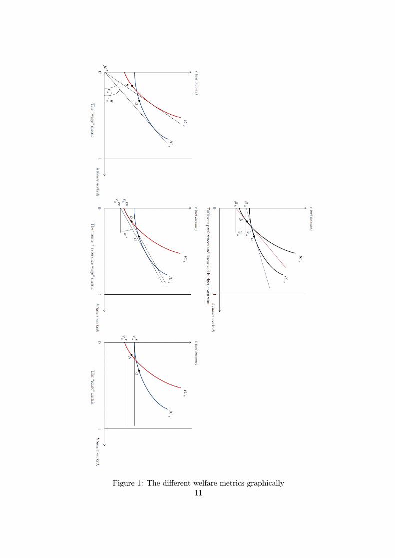
Figure 1: The di¤erent welfare metrics graphically11

In order to estimate the model, we assume the error term to follow an extreme

value type I distribution and being i.i.d. This results in the well-known conditional

logit framework which can be estimated applying the maximum likelihood method.

Data, selection and methodology For our empirical application, we focus on a

selection of 11 European countries and the US. For each country we use microdata for

years 1998 or 2001, except the US, for which we have data from 2006. The datasets

are standard household surveys and contain information on income and the socio-

demographic characteristics needed to perform estimations of labour supply. We

focus on the subpopulation of married couples and hold the labour supply of the

husband �x, while only keeping husbands that at least work full-time (30 hours or

more). This can be justi�ed with the fact, that labour supply behaviour of married

women is well-known to be particularly important. Since this is a rather broad

�nding across countries and might also be due to preferences over leisure and work,

married women are of special attractivness to our purpose. Considered women are

aged between 18 and 59 and are neither disabled nor retired nor in education. We

make use of a discretization of J = 7 hours categories with non-participation, two

part-time, two full-time and two over-time categories.17 Female wages are taken from

observed market wage information for the working women and are imputed using a

common wage estimation with selection correction for the unemployed. Hence, with

view to our model, we are estimating preferences of married women over household

consumption and female leisure time.18

Net income, which in the given static framework equals consumption ci must be

computed at each possible discrete hours choice j = 1; :::; J and is calculated on

basis of all household earnings and non-labour income. Naturally, this requires to

compute all taxes and social security contributions to be paid and social bene�ts to

be received at each of the discrete hours categories as well. This computational work

is performed using EUROMOD, an integrated tax-bene�t calculator for Europe, and

NBER�s tax-bene�t simulator TAXSIM for the US. By now EUROMOD allows to

reproduce the tax-bene�t systems of EU-15 countries for years 1998 and 2001 and

for 4 New Member States for the year 2005. TAXSIM does the same principally

17In particular, the possible choices are from 0 to 60 hours per week with a step of 10 hours.18Note that by this de�nition we treat the household as an individual which makes our empir-

ical approach directly compatible with the theoretical framework presented for individuals in theprevious section.

12

for a range of years using the CPS�IPUMS data.19 The main advantage with EU-

ROMOD is that it provides the microdata across countries in a homogenized way

with respect to variable de�nitions and income concepts and therefore allows for a

common approach in estimation and a comparable analysis of results.

4 Results

This section explains the empirical results in three steps. First, some descriptive

information on the data used is presented. Second, we outline the results from es-

timating individual and cross-country speci�c preference heterogeneity. The third

part constitutes our main analysis and presents information on cross-country order-

ings of the di¤erent individual welfare measures.

4.1 Descriptive information

First of all, we present some descriptive statistics. The �rst two colums of Table

1 show the country and the respective year of the data used. We then present

average monthly household net income as well as average working hours for males

and females and womens participation rates. Note that due to our sample selection

and model de�nition, a large part of the household�s monthly non-labour income

consits of the husband�s labour income. Monetary values are de-/in�ated to the

reference year 2001 and transferred into comparable real values by use of Purchasing

Power Pareties (PPP).

As one might expect, couple households from the US show the highest net in-

come (4841 PPP-USD) and both males and females clearly work above weekly av-

erage hours across countries (44:56 and 27:70 hours/week on average respectively).

However, females from the Nordic countries (Denmark, Finland, Sweden) show the

highest inclination to work (all above 30 hours/week and participation rates larger

than 80%) and also Portuguese married women - the well-known exception out of

the Southern European countries - tend to work more than US females - even though

19For further information on EUROMOD see Sutherland (2007). Country reports are alsoavailable with detailed information on the input data, the tax-bene�t rules and calculation modelingand the validation at the national level, see http://www.iser.essex.ac.uk/research/euromod. Anintroduction to TAXSIM is given by Feenberg and Coutts (1993).

13

Table 1: Income and employment statistics

Country Data Net Non-labour Fem. Part. Female Maleyear income income rate hours hours

AT 1998 3441 2737 0.60 17.94 42.73BE 2001 3770 2833 0.77 25.09 41.93DK 1998 3543 2508 0.84 30.17 42.24FI 1998 2835 1930 0.85 32.28 41.41FR 2001 3175 2346 0.72 23.75 40.14DE 1998 3043 2384 0.64 19.69 39.57IE 2001 4096 3170 0.63 19.28 42.32NL 2001 3735 2951 0.71 18.22 41.46PT 2001 2370 1696 0.76 28.21 42.06UK 1998 3594 2670 0.75 23.09 44.19SW 2001 3268 2256 0.92 31.30 40.51US 2006 4841 3582 0.71 27.20 44.56

Note: The whole sample consits of 43033 married households while the husband at leastis working 30 hours. Non-labour income includes labour income of the husband. Incomesare average monthly values, hours are averages per week. Income values are in realterms: PPP-adjusted USD for 2001. Source: Own calculations based on EUROMOD

and TAXSIM.

their household income is the lowest across countries. In contrast, women from Ire-

land, Austria and the Netherlands work relatively little. While Ireland shows one of

the lowest female participation rates in the sample, it ranks seconds in terms of net

income, mainly due to high male hours. Furthermore, the relatively low household

income in Germany is remarkable. This however becomes explicable when consider-

ing females low participation rate and both females and males relatively low average

hours. France ranks in the middle according to most of the categories and the United

Kingdom shows hard working males but rather less working women.

Yet, these di¤erences do not necessarily say something about di¤erent prefer-

ences. Di¤erences in hours worked and net income are of course also due to dif-

ferences in budget constraints. This is as more true for our sample, where the

husbands income fully enters the non-labour income of the household and we are

only interested in females preferences. In the next section, we therefore provide

distinct preference information, retreived from the estimation of the labour sup-

ply model described in the previous section, and compare the �ndings across the

di¤erent countries.

14

4.2 Estimated preference heterogeneity

In this section we present estimation results for the Box-Cox utility function pre-

sented above, separately retreived for each country. Rather than presenting full

estimation tables for all countries at this stage, we restrict our presentation to a

preference key information, namely the Marginal Rate of Substitution (MRS) be-

tween net income and leisure, computed at a �xed bundle in order to exclusively

capture the shape of di¤erent preference structures rather than di¤erences in (non-

labour) income or leisure.20 In Table 2 we present accordant average values of MRS

of the whole sample of households from all countries according to the taste shifters

that entered our utility function. We �nd that the compensation needed in income

to outweigh one additional hour of work is clearly higher for subgroups like women

with young children or low educated people compared to the overall average. In

particular, the MRS of women with children younger than 3 years old is about one

third higher compared to the MRS of the whole sample. MRS are declining in age

of children and level of education, ending up with a lower MRS of high educated

women compared to the whole sample. Women living in the capital region of a

country have a slightly higher inclination to work. We conclude that on average,

across individuals and countries, each of the characteristics shows a clear direction

for its shifting of tastes.

Based on the preferences estimated, Table 3 reveals that MRS di¤er substantially

across countries, meaning that the compensation needed (in real terms) to o¤set

one additional hour of work varies remarkably. For example, the average MRS for

married women in Germany is almost three times higher compared to that of their

counterparts in Sweden or Finland and more as twice as high for women in Austria

compared to females in the US. Ireland, Austria and the Netherlands clearly show

the highest MRS of married women on average, followed by Germany and the UK.

The Nordic countries, Portugal, Belgium and the US build the sample with the

lowest MRS on average. France again can be seen as lying in between.

These results are much in line with what one might expect from Table 1 above.

Although there is no hint to conclude from the observed descriptive information

directly on the absolute and relative size of the average MRS, di¤erences across

countries tend to be quite sensible. Of course, the di¤erences in MRS across coun-

tries can still be biased by the in�uence of the taste shifters. To better assess this

20The complete estimation results can be found in the appendix.

15

Table 2: MRS according to characteristics

MRS Standard errorWhole sample 9.6 5.4Region 8.6 5.7Children younger 3 15.2 6.5Children between 4 and 6 14.9 6.8Children between 7 and 12 11.9 5.8Low education 13.5 6.1Medium education 9.8 5.2High education 8.3 4.8Women younger 25 8.3 5.2Women between 25 and 55 9.8 5.5Women older than 55 8.4 4.1

Note: MRS are calculated for a �xed bundle (c; h) = (450; 40) and averaged. Incomevalues are in real terms (2001 PPP-USD). Source: Own calculations based on

EUROMOD and TAXSIM.

in�uence, we regress the individual MRS on the several characteristics, including

dummies for the countries (taking Germany as a reference). The results presented

in Table 4 con�rm our precedent �ndings. Coming from Ireland, Austria or the

Netherlands results in a positive e¤ect on the MRS. For example, with Austria as

the country of origin, the MRS will c.p. increase by 4.64 PPP-USD compared to

having Germany as home country. With all other countries the MRS again decreases

c.p., while Nordic countries show the largest negative values. The e¤ect of the other

socio-demographic characteristics is in line with our former �ndings, too. All e¤ects

appear as statistically signi�cant.

4.3 Cross-country welfare orderings

In this section, we empirically compute the welfare metrics according to the formu-

las derived in section 2. Note �rst, that we focus on individual welfare metrics, i.e.

for each household in our sample we individually compute all di¤erent welfare met-

rics based on the accordant individual preference structure retrieved. At no point

throughout the analysis we aggregate individual well-being using some kind of a

social welfare function nor do we add up the metrics for use of a certain inequality

16

Table 3: MRS across countries

Country MRS Standard errorAT 17.7 7.1BE 7.9 2.3DK 4.9 0.5FI 3.7 0.5FR 9.5 3.0DE 12.8 7.8IE 19.7 8.3NL 14.1 5.4PT 5.0 1.3UK 10.7 5.0SW 3.7 0.5US 8.3 3.9

Note: MRS are calculated for a �xed bundle (c; h) = (450; 40) and averaged. Incomevalues are in real terms (2001 PPP-USD). Source: Own calculations based on

EUROMOD and TAXSIM.

index, for example. We completely keep their ordinal character and present results

solely by means of orderings. Second, we calculate expected welfare metrics. More

precisely, we take 300 draws from the extreme value type I distribution of the error

term and identify for each draw the discrete category which gives the maximum

utiliy. This utility is averaged over all 300 draws and the resulting expected utility

inserted into the formulas for the welfare metrics. Calcualtion follows by use of ana-

lytical or numerical procedures depending on the metric. We furthermore calculate

accordant expected net income and expected hours worked.

First of all, consider Figure 2. It shows empirical rank correlations for the indi-

vidual ordering positions in the percentile distribution of the di¤erent metrics for the

whole sample (with the �rent�metric always located on the x-axis). The di¤erences

in the evaluations of individual well-being are obvious. While the upper-left panel

still reveals quite a strong correlation between the individual ordering positions un-

der the pure income and the �rent�metric, this correlation sequentially decreases

when taking preferences for leisure more and more into account. In the bottom-

right panel, the correlation is almost not existent anymore, showing the relatively

highest transitions between the di¤erent ordering positions under the �rent� and

the �wage�metric. This result con�rms the �nding of Decoster and Haan (2010)

17

Table 4: MRS regressed on characteristics and country dummies

MRS Coe¢ cient Standard errorCountry dummies (ref. DE)AT 4.64��� 0.10BE -5.98��� 0.09DK -8.44��� 0.10FI -9.20��� 0.12FR -4.42��� 0.04IE 5.67��� 0.16NL 0.41��� 0.07PT -9.87��� 0.10UK -1.96��� 0.05SW -9.09��� 0.10US -4.49��� 0.04Region -1.28��� 0.03Children younger 3 7.11��� 0.03Children between 4 and 6 5.72��� 0.03Children between 7 and 12 2.80��� 0.03Low education 4.62��� 0.04Medium education 1.23��� 0.03Age wife 0.06��� 0.00Age husband 0.40��� 0.03Constant 4.93��� 0.07N obs. 43033R2 0.80Prob>F 0.00

Note: ***p<0.01, **p<0.05, *p<0.1Source: Own calculations based on EUROMOD and TAXSIM.

for Germany with data from 2005 for a broader set of observations. Also, it seems

natural that the di¤erences in the correlation plots are due to the treatment of

preference heterogeneity under the di¤erent metrics.

In a next step, we also want to identify the specifc drivers of that preference het-

erogeneity, more precisely, whether it is likely to observe households from a certain

country being over- or under-represented in certain parts of the distribution of the

measures. If so, can this be expected from the preference information derived in the

previous subsection? What is the e¤ect on a cross-country comparison of individual

well-being? The answers to these questions are illustrated in Tables 5-8 and Figure

18

3.

Figure 2: Rank correlations of empirical welfare metrics

Table 5 shows the share of the countries sample population in the bottom quin-

tile of several welfare distributions. In the second column, the weighted share of a

countries population within the sample population of all countries together is given.

Going through the columns to the right, the di¤erent welfare criteria from the pure

income measure up to the �wage�metric are listed. If the welfare levels were uni-

formly distributed across countries, we would observe exactly the population share

in each cell (as by chance Austria for the pure income measure). However, due

to cross-country di¤erences we at least expect some variation in the quintiles. As

pointed out in the normative section, the �rent�metric can be interpreted as hold-

ing individuals minimally responsible for their preferences for leisure, while for the

�wage�metric it holds the other way round - here, we consider individuals as being

maximally responsible for their distaste to work. When focussing on the group of

Nordic countries, for example, where married women show a sound inclination to

work, we notice that relative to its population share of 1; 01% Finland is clearly

over-represented in the bottom quintile of the income distribution (1; 74%), while

Sweden and especially Denmark are under-represented (1; 69 vs. 1; 18% and 1; 42

19

vs 0; 56% respectively). But when moving to the bottom quintile of the �rent�met-

ric, the share of households clearly decrease compared to the income distribution

for all three countries (0; 62%, 0; 28% and 0; 14% respectively in the same order).

The reason is, that households from the Nordic countries are now pushed out of the

bottom of the distribution by households from countries as Austria, Ireland or the

Netherlands, where it holds exactly the other way round and women do not work

as much. Under the �rent�measure this distaste is only assigned minimal respon-

sibility and we end up with considering households from these countries as being

particularly needy. When moving through the three �rent + reference wage�criteria

(with increasing reference wage values) up to �wage�metric, the pattern changes

once again and we observe striking rank reversals. Now, households in the Nordic

countries are clearly over-represented in the bottom quintile (3; 75%, 4; 11% and

1; 80% respectively) while households in the countries of our �counterpart�selection

(AT, IE, NL) are under-represented.

For most of the countries and metrics, a clear tendency in the orderings emerges

in line with the preferences retrieved. A further remarkable example is the US due

to its high population share. It follows the same direction as the Nordic countries

and we observe 31% of US households in the bottom quintile of the �rent�metric

vs. 38% for the �wage�metric, a di¤erence of 7 percentage points or 14; 6% of its

sample population share. Table 6 then shows the top quintile of the distribution for

the di¤erent metrics. Hence it must be read in the �opposite�logic and results are

in line with what we expect from our investigation of Table 5.

However, an assessment only on basis of the �rst and the �tfth quintile could be

misleading, at least it is incomplete. Sound changes might occur only at the second

or fourth quintile. Notice furthermore that it is indeed not only heterogeneity in

preferences that determines the ordering of the individuals but also di¤erences in the

bundles (choices) and thereby (non-labour) income which can substantially in�uence

if and where individual indi¤erence curves cross.21 Therefore, Table 7 combines the

information from all quantiles of a welfare ordering and shows the average individual

percentile position for each country for the di¤erent welfare metrics. Nevertheless,

the main �ndings from Tables 5 and 6 can be con�rmed and are sometimes even

clearer now. For example, households from the US on average rank at the 61st

percentile position in the overall income distribution while for the �rent�metric

21This aspect will be discussed further in section 5.

20

Table 5: Composition of the 1st quintile of the welfare ordering for the di¤erentmetrics

Country Share Income Rente RW p25 RW p50 RW p75 Wage

AT 0.0161 0.0161 0.0240 0.0064 0.0051 0.0053 0.0042BE 0.0190 0.0053 0.0065 0.0117 0.0149 0.0186 0.0107DK 0.0142 0.0056 0.0014 0.0056 0.0053 0.0042 0.0180FI 0.0101 0.0174 0.0062 0.0295 0.0313 0.0320 0.0375FR 0.1334 0.2093 0.2384 0.2242 0.2253 0.2220 0.1830DE 0.1567 0.2537 0.2372 0.1789 0.1784 0.1773 0.1693IE 0.0057 0.0023 0.0033 0.0007 0.0005 0.0005 0.0007NL 0.0401 0.0197 0.0256 0.0142 0.0151 0.0182 0.0120PT 0.0155 0.0532 0.0590 0.0651 0.0671 0.0697 0.0608UK 0.0944 0.0927 0.1081 0.0895 0.0901 0.0951 0.0792SW 0.0169 0.0118 0.0028 0.0300 0.0320 0.0330 0.0411US 0.4779 0.3129 0.2874 0.3442 0.3349 0.3240 0.3834

Note: Reference wages for the �rent + reference wage�metric are the 25th, 50th and75th percentile values over all countries. Source: Own calculations based on EUROMOD

and TAXSIM.

the position slightly increases to the 62nd percentile on average. But when moving

to the �wage�metric they rank only at the 54th percentile anymore. The same

direction of movement especially holds for the Nordic countries considered before,

while the opposite tendency is again true for Austria, Ireland and the Netherlands

but also France, Germany and the UK. Households from all these countries rank

considerably better under the �wage� criterion compared to the �rent�metric as

the women�s wage rate needed to be compensated for the corresponding increase in

labour supply in that hypothetical case would be relatively high.

Furthermore, Table 7 shows one additional feature which is the di¤erences in

the average ordering positions across countries when reading it vertically. It is

far away from showing di¤erent rankings of countries in terms of household well-

being but at least it reveals rank reversals on average due to cross-country preference

heterogeneity for the given sample population. This information is further illustrated

with help of Figure 3. Countries are ordered from the highest to the lowest average

household position in the income distribution, shown by the �rst, black bar. The

following bars show the average positions for the subsequent metrics which makes

easier both a comparison within one as well as across di¤erent countries. Clearly,

couple households from the US �rank� highest in terms of the average percentile

21

Table 6: Composition of the 5th quintile of the welfare ordering for the di¤erentmetrics

Country Share Income Rente RW p25 RW p50 RW p75 Wage

AT 0.0161 0.0083 0.0061 0.0101 0.0114 0.0157 0.0244BE 0.0190 0.0108 0.0080 0.0117 0.0102 0.0073 0.0073DK 0.0142 0.0042 0.0103 0.0048 0.0043 0.0039 0.0013FI 0.0101 0.0008 0.0020 0.0005 0.0004 0.0003 0.0001FR 0.1334 0.0487 0.0347 0.0489 0.0480 0.0438 0.0513DE 0.1567 0.0359 0.0240 0.0583 0.0742 0.1147 0.1762IE 0.0057 0.0061 0.0058 0.0066 0.0082 0.0124 0.0159NL 0.0401 0.0227 0.0119 0.0344 0.0454 0.0611 0.0874PT 0.0155 0.0058 0.0037 0.0039 0.0025 0.0009 0.0027UK 0.0944 0.0601 0.0434 0.0652 0.0705 0.0731 0.0833SW 0.0169 0.0037 0.0056 0.0035 0.0032 0.0027 0.0018US 0.4779 0.7930 0.8444 0.7522 0.7217 0.6643 0.5483

Note: Reference wages for the �rent + reference wage�metric are the 25th, 50th and75th percentile values over all countries. Source: Own calculations based on EUROMOD

and TAXSIM.

position in the income distribution while this position is taken over by households

from Denmark when moving to the �rent� criterion ( - even though the average

position for the US increases as well). But women in Denmark show an even more

pronounced inclination to work compared to US females. Finally, for the �wage�

metric, US women rank only 4th anymore while the �fall� of Danish households

is even more dramatic (from 1 to 9). The highest average ranks are now taken

over by households from Ireland, the Netherlands and Austria. Not least, Figure

3 also illustrates the importance of the absolute monetary value of the measures,

too. Couples from Portugal for instance are as worse o¤ in terms of income such

that considering preference heterogeneity hardly changes anything, at least in a

cross-country perspective.

In sum, one can carefully cluster households from certain countries into di¤erent

groups. Couples from the Nordic countries and the US clearly perform better un-

der criteria that assign minimal or low responsibility to women�s aversion to work

while households from the Anglo-Saxon and some Continental European countries

(including Germany and France) perform better (i.e. are considered less needier)

under criteria that include high or maximal responsibility for a greater distaste for

work of females.

22

Table 7: Weighted average percentile position in the global distribution of the welfareordering for the di¤erent metrics

Country Income Rente RW p25 RW p50 RW p75 Wage

AT 44.41 38.05 52.16 55.85 59.34 64.87BE 52.80 50.17 49.58 46.95 43.09 47.60DK 48.91 63.04 48.04 46.94 47.16 33.35FI 31.72 44.23 22.88 21.34 20.50 15.80FR 37.94 34.40 37.28 36.98 36.73 40.62DE 36.11 36.03 42.52 44.88 47.85 51.16IE 57.41 55.23 61.46 66.79 73.75 75.78NL 52.22 47.61 58.50 60.44 62.50 69.19PT 20.73 15.32 11.95 10.11 7.63 14.68UK 47.04 44.00 48.05 48.30 48.31 51.22SW 42.19 51.00 33.74 32.04 31.02 26.78US 60.99 62.40 58.96 58.16 57.17 53.78

Note: Reference wages for the �rent + reference wage�metric are the 25th, 50th and75th percentile values over all countries. Source: Own calculations based on EUROMOD

and TAXSIM.

Again, as with the assessment of the MRS across countries above, the orderings

across countries are also caused by the in�uence of socio-demographic characteristics

other than country membership. We therefore run multivariate regressions of the

metrics on the characteristics to better assess the signi�cance of the origin. More

precisely, we take the individual percentile position and regress on socio-demographic

characteristics and each country dummy seperately. This way, we can better inter-

prete the distinct e¤ect of the origin for each country and interpret it in terms of

moving by percentage points in the ordering of the speci�c metric. Thus, we end up

with 12 di¤erent regression equations of which the country e¤ects are summarized

in Table 8. In brief, we �nd strong and signi�cant evidence for the observed country

di¤erences in welfare orderings.

5 Discussion

Our results drawn from the previous section clearly suggest that preference hetero-

geneity matters substantially when evaluating individual welfare - not only within

but also across countries. The exemplary empirical illustration for a set of European

23

020

4060

80

US IE BE NL DK UK

Income Rent RW1 RW2 RW3 Wage

020

4060

AT SW FR DE FI PTSource: Own calculations based on EUROMOD and TAXSIM

Figure 3: Comparison of average individual percentile position in ordering of di¤er-ent metrics

countries and the US suggest, that when taking into account non-market dimensions

of individual well-being, one should be cautious towards the decision of how to treat

preference heterogeneity. Assessment of individual welfare might di¤er substantially

under di¤erent normative choices for certain criteria (including net income as well,

which of course is also a choice in terms of how to treat individual preferences).

Besides many advantages, our illustration for the leisure-consumption context us-

ing discrete choice labour supply models has shortcomings as well. Some of these

aspects are discussed in the following paragraphs.

Constraints vs. preferences This paragraph critically discusses the problem of

identifying the in�uence of constraints versus that of preferences on the empirical

behaviour of the welfare metrics. This amounts to a more general discussion of

how to seperate e¤ects of �real� constraints on the one hand from that of �real�

preferences on the other hand in (structural) empirical work.

[To be completed.]

24

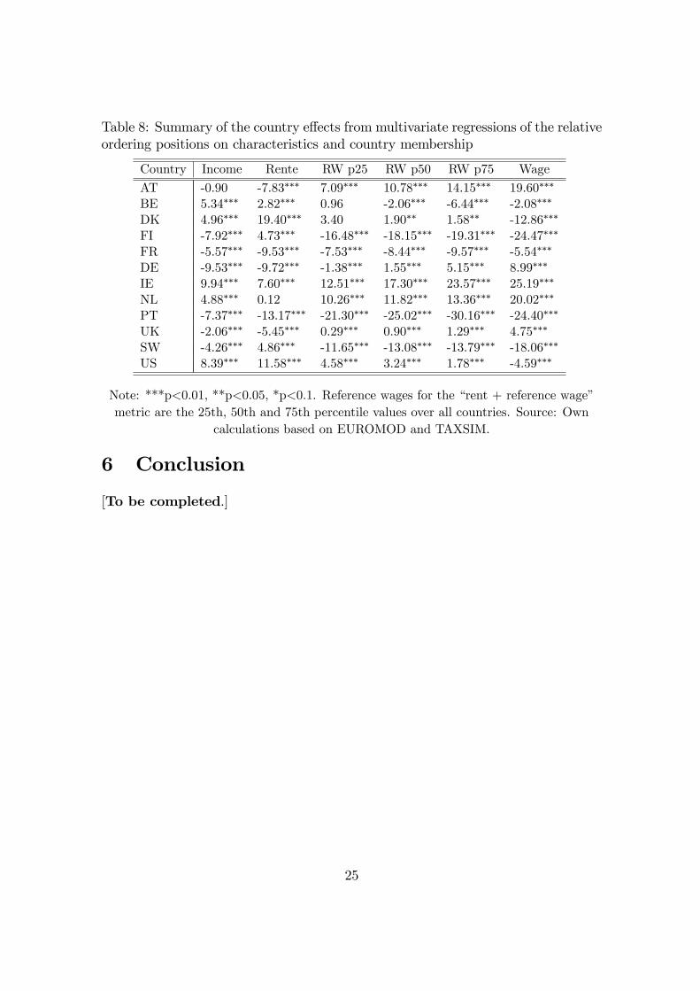
Table 8: Summary of the country e¤ects from multivariate regressions of the relativeordering positions on characteristics and country membership

Country Income Rente RW p25 RW p50 RW p75 Wage

AT -0.90 -7.83��� 7.09��� 10.78��� 14.15��� 19.60���

BE 5.34��� 2.82��� 0.96 -2.06��� -6.44��� -2.08���

DK 4.96��� 19.40��� 3.40 1.90�� 1.58�� -12.86���

FI -7.92��� 4.73��� -16.48��� -18.15��� -19.31��� -24.47���

FR -5.57��� -9.53��� -7.53��� -8.44��� -9.57��� -5.54���

DE -9.53��� -9.72��� -1.38��� 1.55��� 5.15��� 8.99���

IE 9.94��� 7.60��� 12.51��� 17.30��� 23.57��� 25.19���

NL 4.88��� 0.12 10.26��� 11.82��� 13.36��� 20.02���

PT -7.37��� -13.17��� -21.30��� -25.02��� -30.16��� -24.40���

UK -2.06��� -5.45��� 0.29��� 0.90��� 1.29��� 4.75���

SW -4.26��� 4.86��� -11.65��� -13.08��� -13.79��� -18.06���

US 8.39��� 11.58��� 4.58��� 3.24��� 1.78��� -4.59���

Note: ***p<0.01, **p<0.05, *p<0.1. Reference wages for the �rent + reference wage�metric are the 25th, 50th and 75th percentile values over all countries. Source: Own

calculations based on EUROMOD and TAXSIM.

6 Conclusion

[To be completed.]

25

A Appendix:

[To be completed.]

26

References

Aaberge, R., Colombino, U. and Strøm, S. (2000). Labor Supply Responses and

Welfare E¤ects from Replacing Current Tax Rules by a Flat Tax: Empirical

Evidence from Italy, Norway and Sweden, Journal of Population Economics

13(4): 595�621.

Aaberge, R., Colombino, U. and Strøm, S. (2004). Do more equal slices shrink

the cake? An empirical investigation of tax-transfer reform proposals in Italy,

Journal of Population Economics 17: 767�785.

Aaberge, R., Dagsvik, J. and Strøm, S. (1995). Labor Supply Responses and Welfare

E¤ects of Tax Reforms, Scandinavian Journal of Economics 97(4): 635�659.

Alesina, A., Glaeser, E. and Sacerdote, B. (2005). Work and Leisure in the United

States and Europe: Why So Di¤erent?, NBER Macroeconomics Annual 20: 1�64.

Bargain, O., Orsini, K. and Peichl, A. (2010). Labor Supply Elasticities in Europe

and the US, mimeo.

Becker, G. S., Philipson, T. J. and Soares, R. R. (2005). The Quantity and Quality

of Life and the Evolution of World Inequality, Amercian Economic Review

95: 277�291.

Blanchard, O. (2004). The Economic Future of Europe, Journal of Economic Per-

spectives 18: 3½U26.

Blundell, R., Duncan, A., McCrae, J. and Meghir, C. (2000). The Labour Market

Impact of the Working Families�Tax Credit, Fiscal Studies 21(1): 75�104.

Boadway, R., Marchand, M., Pestieau, P. and Del Mar Racaniero, M. (2002). Op-

timal Redistribution with Heterogeneous Preferences for Leisure, Journal of

Public Economic Theory 4: 475�498.

Boarini, R., Johansson, A. and d�Ercole, M. M. (2006). Alternative Measures of

Well-Being, OECD Social, Employment and Migration Working Papers 33.

Choné, P. and Laroque, G. (2009). Optimal taxation in the extensive model, mimeo.

27

Choné, P. and Laroque, G. (2005). Optimal incentives for the labor force participa-

tion, Journal of Public Economics 89: 395�425.

Decoster, A. and Haan, P. (2010). Empirical welfare analysis in random utility

models of labour supply, KU Leuven, CES Discussion Paper Series 10.30.

Feenberg, D. R. and Coutts, E. (1993). An Introduction to the TAXSIM Model,

Journal of Policy Analysis and Management 12(1): 189�194.

Fleurbaey, M. (2006). Social welfare, priority to the worst-o¤ and the dimensions

of individual well-being, in F. Farina and E. Savaglio (eds), Inequality and

Economic Integration, London: Routledge.

Fleurbaey, M. (2007). Social Choice and the Indexing Dilemma, Social Choice and

Welfare 29: 633�648.

Fleurbaey, M. (2008a). Fairness, Responsibility and Welfare, Oxford University

Press.

Fleurbaey, M. (2008b). Willingness-to-pay and the equivalence approach, OPHI

Working Paper No. 25.

Fleurbaey, M. (2009). Beyond GDP: The Quest for a Measure of Social Welfare,

Journal of Economic Literature 47: 1029�1075.

Fleurbaey, M. and Gaulier, G. (2009). International Comparisons of Living Stan-

dards by Equivalent Incomes, Scandinavian Journal of Economics 111: 597�624.

Fleurbaey, M. and Maniquet, F. (2006). Fair Income Tax, Review of Economic

Studies 73(1): 55�83.

Fleurbaey, M. and Trannoy, A. (2003). The Impossibility of a Paretian Egalitarian,

Social Choice and Welfare 21: 243�263.

Hodler, R. (2008). Leisure and Redistribution, European Journal of Political Econ-

omy 24: 354�363.

Hodler, R. (2009). Redistribution and Inequality in a Heterogeneous Society, Eco-

nomica 76: 704�718.

28

Jacquet, L., Lehmann, E. and Van der Linden, B. (2010). Optimal Redistributive

Taxation with both Extensive and Intensive Responses, IZA DP No. 4837.

Jones, C. I. and Klenow, P. J. (2010). Beyond GDP? Welfare across Countries and

Time, NBER Working Paper 16352.

Kassenboehmer, S. C. and Schmidt, C. M. (2011). Beyond GDP and Back: What

is the Value-Added by Additional Components of Welfare Measurement?, IZA

Discussion Paper No. 5453.

King, M. (1983). Welfare e¤ects of tax reforms using household data, Journal of

Public Economics 21: 183�214.

Oohge, E. and Peichl, A. (2010). Fair and E¢ cient Taxation under Partial Control:

Theory and Evidence, IZA Discussion Paper No. 5388.

Pencavel, J. (1977). Constant-Utility Index Numbers of Real Wages, The American

Economic Review 67(2): 91�100.

Prescott, E. C. (2004). Why Do Americans Work So Much More Than Europeans?,

Federal Reserve Bank of Minneapolis Quarterly Review 28(1): 2�13.

Preston, I. andWalker, I. (1999). Welfare measurement in labour supply models with

nonlinear budget constraints, Journal of Population Economics 12(3): 343�361.

Saez, E. (2001). Using elasticities to derive optimal income tax rates, Review of

Economic Studies 68(1): 205�229.

Saez, E. (2002). Optimal income transfer programs: intensive versus extensive labor

supply responses, Quarterly Journal of Economics 117(3): 1039�1073.

Stiglitz, J., Sen, A. and Fitoussi, J.-P. (2009). Report by the Comission on the

Measurement of Economic Performance and Social Progress, Technical Report.

Sutherland, H. (2007). Euromod: the tax-bene�t microsimulation model for the

European Union, in A. Gupta and A. Harding (eds), Modelling Our Future:

Population Ageing, Health and Aged Care, Vol. 16 of International Symposia in

Economic Theory and Econometrics, Elsevier, pp. 483�488.

Van Soest, A. (1995). Structural Models of Family Labor Supply: A Discrete Choice

Approach, Journal of Human Resources 30(1): 63�88.

29

Weinzierl, M. (2009). Incorporating Preference Heterogeneity into Optimal Tax

Models: De Gustibus non est Taxandum, mimeo.

30