Voting, Taxes and Heterogeneous Preferences:Evidence from Swedish Local Elections*

Eva Mörk§ Mattias Nordin¶

Abstract

A standard �nding in the literature on political agency is that voters punish incumbentswho raise taxes. Typically, only the reaction of a representative voter is considered, with thenotion that all voters dislike high taxes because the revenue is, at least on the margin, spenton rent-seeking activities. In this paper we question this interpretation by considering theheterogeneous responses to tax changes in the electorate. Using high-quality panel surveydata from Swedish local politics we �nd that voters who, ex ante, prefer a small public sectorpunish incumbents who raise taxes, while voters who prefer a large public sector actuallyreward tax hikes. This result holds also conditional on individuals’ past voting behavior andfor voters who have low con�dence in politicians, indicating that Swedish voters interprettax changes based on their own policy preferences, rather than as going to wasteful activities.

Keywords: Electoral accountability, local taxation, voter preferences, political agency

JEL Classi�cation: D72, H71

*We are grateful for comments from Sören Blomquist, Massimo Bordignon, Matz Dahlberg, Richard Friberg andGisle J. Natvik and from seminar participants in Helsinki, Stockholm, Uppsala and Umeå and conference participantsat the IV Workshop on Fiscal Federalism in Barcelona, the 68th Annual Congress of the IIPF in Dresden, the Jørn-Rattsø’s 60-Anniversary-Workshop in Trondheim, the Empirical Political Economics and Political Science Workshopin Helsinki and the Nordic Workshop in Tax Policy and Public Economics in Oslo. We also thank Jonas Klarin forexcellent research assistance. Financial support from the Swedish Research Council (grant number 2011-2096) isgratefully acknowledged.

§Department of Economics, UCFS and UCLS, Uppsala University, IEB, IZA, CESifo¶Department of Statistics and UCFS, Uppsala University

1

1 Introduction

In representative democracies, voters have delegated the responsibility to implement public poli-cies to elected politicians. Ideally, voters would like these politicians to implement policies thatare in the voters’ best interest. However, it is not possible for voters to perfectly control whatpoliticians will do once they are elected, and politicians cannot always commit to a policy plat-form before an election. Also, voters have limited knowledge of the intentions and preferencesof the politicians. By instead conditioning the decision to reelect the incumbent on past pol-icy outcomes, voters can incentivize good behavior and weed out incompetent politicians. Asa consequence, even rational and forward-looking voters may base their vote decisions on theincumbent’s past behavior in o�ce.

There is also vast empirical evidence that voters do react to past policies at the election booth.In a in�uential paper, Peltzman (1992) studies post-World War II U.S. gubernatorial elections and�nds that voters penalize federal and state spending growth, concluding that voters are �scallyconservative. Findings in later empirical work by, e.g., Besley (2006) and Niemi et al. (1995), indi-cate that voters punish U.S. governors for setting high taxes, which is to some extent in line withPeltzman’s conclusion.1 In addition, Besley and Case (1995b) (U.S. states) and Revelli (2002) (U.K.districts) instead �nd that voters punish incumbents for setting higher taxes than politicians inneighboring regions.2 That incumbents will be punished for setting high taxes is also an implicitassumption in the empirical literature analyzing election cycles in public spending and taxes,see, e.g., Kneebone and McKenzie (2001); Andrikopoulus et al. (2004); Dahlberg and Mörk (2011);Foremny and Riedel (2014).

But should we expect all voters to dislike high taxes? Because tax revenues can be spent onvaluable goods and services, are there voters who are in fact more likely to vote for an incumbentraising taxes? To our knowledge, no paper has tested whether this is the case. The aim of thispaper is to investigate such heterogeneous responses to tax changes at the municipal level inSweden. We �nd that voters’ responses to local taxation clearly depend on their preferences forpublic spending. Conditional on how they voted in the last election, we show that voters whoprefer a large public sector is more likely to vote for a ruling coalition who raised taxes during theelection term, while the converse is true for voters who prefer a smaller public sector. Becausethe average reaction to tax changes is close to zero in the electorate, our �ndings suggest thatSwedish voters do not interpret tax hikes as indicative of rent-seeking behavior, but rather asre�ecting ideological di�erences regarding the size of government.

1Lowry et al. (1998) �nd that voters’ responses depend on the political identity of the incumbent; whereas Re-publican candidates are punished for unanticipated increases in the size of the budget, Democrats may actually berewarded.

2See Bordignon et al. (2004) for a theoretical discussion on this type of yardstick competition.

2

Our paper is closely related to the political-agency literature (see Besley 2006 for an excellentoverview). In political-agency models, voters react negatively to high taxes because resourcescollected through taxation is assumed to, at least partly, be wasted, either due to incompetentpoliticians or due to politicians engaging in rent-seeking activities. The argument was �rst putforth by Barro (1973) and Ferejohn (1986) that consider rent-seeking politicians in pure moralhazard models. Voters try to curb rent-seeking activities by conditioning their reelection decisionon the incumbent’s behavior. They do so by choosing an optimal threshold value where theyreelect the incumbent if taxes are lower than that threshold, and vote the incumbent out of o�ceotherwise. In this way, they give rent-seeking politicians incentives to not collect maximumrents.3 Later models developed by Rogo� (1990), Persson and Tabellini (2000) and Besley (2006),among others, extend the analysis by also introducing elements of adverse selection. In a settingwhere some politicians are more competent, or less prone to engage in rent-seeking activities,than others and where voters have imperfect information about politicians’ types, incumbentswill implement policies in order to signal that they are “good”. As a result, in separating equilibra,voters will not reelect “bad” politicians that reveal their type by setting high taxes (or spending).4

Of course, public resources are not only spent on wasteful activities, but can also be usedto supply valuable goods and services. The in�uential citizen-candidate model (Osborne andSlivinsky 1996; Besley and Coate 1997) builds on the premise that politicians hold preferences overthe level of productive public spending, and that their preferences determine policy outcomes.5

Voters would therefore like to elect politicians that implement policies in line with those preferredby the voters. If the politicians’ policy preferences are hidden to voters, a tax increase may bea signal to voters that the incumbent prefers a large public sector. By conditioning reelectiondecisions on past policies, voters may either select politicians with preferences that correspondsto those of the voters, or discipline politicians to implement policies preferred by the voters.6

There are hence two di�erent interpretations for why voters would respond to tax policies.One is that politicians are rent-seeking or incompetent, and that high taxes indicate wastefulor ine�cient public spending. The other is that politicians use taxed resources for productive

3Besley and Case (1995a) �nd that term-limited governors implement di�erent policies (i.e. higher spending andtaxes) which is in line with the moral hazard model.

4Alt et al. (2011) exploit variation in U.S. gubernatorial term limits in order to disentangle accountability andcompetence e�ects. Their �ndings indicate that voters use elections to throw less competent incumbents out ofo�ce. For Swedish municipalities, Pettersson-Lidbom (2006) �nds that governments who are reelected, on averageset lower tax rates compared to those who are voted out of o�ce. He interpret these �ndings from an agencyperspective where high taxes signal rent-seeking behavior.

5That this is the case in Sweden is indicated by empirical evidence in Pettersson-Lidbom (2008). Using a re-gression discontinuity design, he �nds that left-wing local governments spend and tax 2–3% more than right-winggovernments, a di�erence that cannot be attributed to voters’ preferences. His conclusion from these �ndings is thatpoliticians’ preferences indeed matter in the Swedish context.

6Similar arguments are put forth in the theoretical models by, e.g., Alesina and Cukierman (1990); Cukiermanand Tommasi (1998); Schultz (2002) and Acemoglu et al. (2013).

3

public spending, and that voters’ reactions depend on to what extent the level of public spendingand taxes corresponds to the preferences of the voters. In order to separate between these twopotential explanations, one would ideally like to have data on both the level and quality of publiclyprovided services together with taxation data. However, reliable data on quality is typically notavailable, and using the level of spending as a proxy for quality is not satisfactory since such datacannot capture how e�ciently public goods and services are provided.

In this paper, we approach the question from a slightly di�erent angle. Speci�cally, if taxedresources are wasted, we would expect voters to uniformly dislike tax hikes. On the other hand, ifthe resources are used for productive public spending, we would expect heterogeneous responsesamong voters, depending on their preferences. That is, voters who prefer a large governmentsector might actually reward an incumbent that raised taxes the previous term. To distinguish be-tween the two competing views, we will test whether such heterogeneous responses exist amongSwedish voters. To do so, we rely on Swedish survey data containing information about voters’preferences, as well as information on how the respondents state that they cast their votes in localgovernment council elections. Thanks to the panel dimension of the data, where each respondentis surveyed in connection to two consecutive elections, we are able to i) compare voters’ prefer-ences at the beginning of an election term with ii) the policies implemented by the incumbentwhile in o�ce and, iii) with the same voters’ responses to these policies in the elections at theend of the election term. We are also able to control for which party the voter voted for in thepast election, implying that we identify the e�ect from changes in voting behavior. In this waywe can empirically investigate whether citizens with preferences for a large public sector are lessprone to punish incumbents for setting high taxes than voters with preferences for a small publicsector. Our data cover the period 1982–2006, during which eight local elections took place in 269Swedish municipalities.

We �nd that voters’ preferences for public spending clearly matter for how voters react totax changes. While voters on average do not seem to dislike taxes, there is a large heterogene-ity among them. Voters who prefer a smaller government sector are less likely to vote for anincumbent who raised taxes the previous election term, while voters who prefer a large govern-ment sector actually rewards tax increases. This result stands in contrast with the �ndings inthe agency literature, suggesting that voters in Sweden do not consider tax hikes as indicative ofrent-seeking activities, but rather as re�ecting di�erent policy positions.

The remainder of the paper is organized as follows: In the next section, we brie�y describethe Swedish setting and the role played by local governments. Section 3 presents our data andsome descriptive analysis, followed by the empirical strategy in section 4. We then present ourempirical results, with the �nal section concluding the paper.

4

2 The Swedish setting

Sweden has a long tradition of strong and autonomous local governments7 that are responsible forsupplying important welfare services such as child care, schooling, care for the elderly and localinfrastructure.8 Personnel costs account for the bulk of municipal expenditures. The municipal-ities �nance their activates through a proportional income tax,9 intergovernmental grants fromthe central government and, to a lesser extent, user fees. Their right to set taxes is establishedin the constitution, and income from these locally set income taxes accounts for approximately60–70% of local government revenues.10 The system of intergovernmental grants transfers re-sources from the central to the local level, as well as between municipalities depending on theirtax bases and cost structures. During the period of our study, there were between 279 and 290municipalities in Sweden, with a median population of 15,600 inhabitants.

The municipalities are governed by a municipal council elected in local proportional elections(held on the same day as the central government election). Elections are held in September ofevery fourth year (until 1994, every third year), and the municipal election is held at the samedate as the national (and county) election. The municipal council sets tax rate and budget forthe upcoming year in the last months of the year. Our data cover the period 1982–2006, whichimplies that we have data from eight local elections. During that time period, the turnout ratehas varied between 78% and 90%.

Sweden is a multiparty-system, with largely the same parties at the local and central levels.These parties are the Left Party, the Social Democrats and the Green Party typically considered asleft-wing parties, and the Centre Party, the Liberals, the Christian Democrats and the Moderates,typically considered as right-wing parties.11 Although there is no formal local government, asubset of parties typically agree on the budget and other important policy decisions. We denotethis subset of parties as belonging to the ruling coalition. The executive branch of the localgovernment is the municipal board. In contrast to the national level, the opposition parties are

7There are two parallel layers of local governments in Sweden, municipalities and counties, where the latter areprimarily responsible for health care. In this paper, we focus on the municipalities.

8Since the 1990’s, private providers of welfare services have been growing in importance. However, even theservices provided by public companies are �nanced by the municipal budget and the private providers are not allowedto charge the user directly if they would like to be reimbursed by the municipality. The public sector remains thedominant provider.

9In addition to the municipal tax rate, which is approximately 20% of labor income, individuals also pay a pro-portional income tax to the counties (approximately 10%). These two taxes are often presented together as themunicipality tax rate (“kommunalskatt”). For labor incomes above a certain threshold, the taxpayer also pays acentral government income tax. In the tax returns, the state and local taxes are presented separately.

10The taxation right was temporarily overridden by a centrally mandated local tax freeze from 1991 to 1993, seebelow.

11Nowadays, the Sweden Democrats play an important role in Swedish politics, but they emerged late duringour studied period and were not, at that time, represented at the national level, and with limited presence in localmunicipal councils.

5

020

40

60

Perc

ent

V S MP C FP KD M Other

020

40

60

Perc

ent

V S MP C FP KD M Other

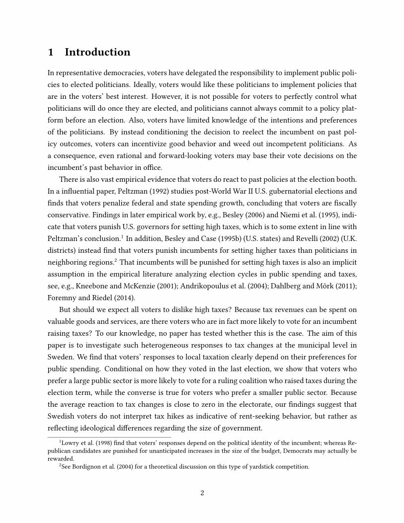
Figure 1: Percent of each party being incumbent

Note: The left panel shows the percent of municipalities in which a given party was part of the ruling coalition. Theright panel shows percent of municipalities in which the chairman of the municipal board came from a given party.The acronyms are: V = Left Party, S = Social Democrats, MP = Green Party, C = Centre Party, FP = Liberals, KD =Christian Democrats, M = Moderates

generally also represented in the municipal board. Typically, the position as chairman of the boardis held by the largest party in the ruling coalition.12 This position is generally considered the mostimportant in municipal politics, equivalent to the mayoral position in many other countries (Folkeand Rickne 2016).

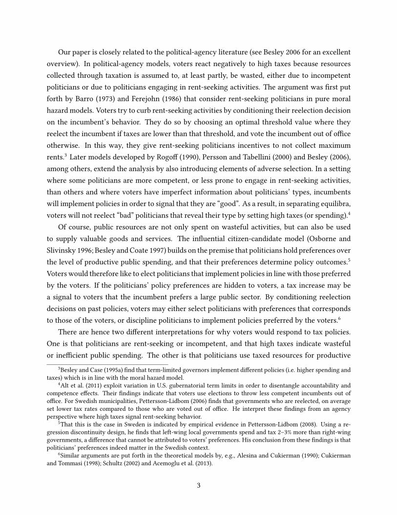
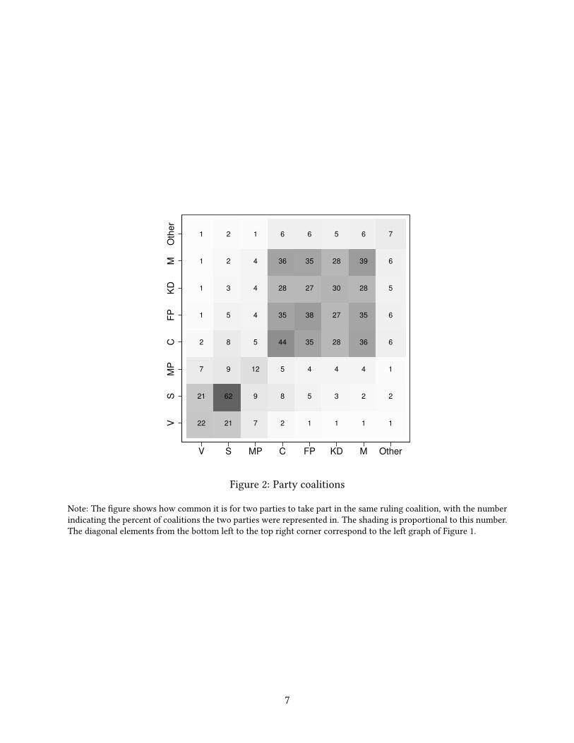
For our empirical analysis, we have compiled data on coalitions as well as the party of thechairman of the board from several di�erent sources, something that is described in more detailbelow. The left graph of Figure 1 shows the percentage of municipalities in which each partyformed part of the ruling coalition. The Social Democrats were the party who, during the studiedperiod, were most likely to belong to a ruling coalition, followed by the four right-wing parties.The right graph shows that the chairman of the municipal board came almost exclusively fromthe Social Democrats, the Centre Party and the Moderates. Figure 2 illustrates that the fourright-wing parties typically formed coalitions with each other, while the most common coalitionpartner for the Social Democrats was the Left Party, followed by the Green Party and the CentreParty. It is worth noting that it is quite common that not all of the parties that are characterizedas left-wing or right-wing take part in a ruling coalition. For example, in around half the caseswhere the Social Democrats were in power, they ruled by themselves. Also, coalitions across theleft-right wing dimension exist: In over 14% of the cases, there was a coalition involving at leastone left-wing and one right-wing party.

12In our data, this is true for over 91% of the municipalities.

6

22 21 7 2 1 1 1 1

21 62 9 8 5 3 2 2

7 9 12 5 4 4 4 1

2 8 5 44 35 28 36 6

1 5 4 35 38 27 35 6

1 3 4 28 27 30 28 5

1 2 4 36 35 28 39 6

1 2 1 6 6 5 6 7

VS

MP

CF

PK

DM

Oth

er

V S MP C FP KD M Other

Figure 2: Party coalitions

Note: The �gure shows how common it is for two parties to take part in the same ruling coalition, with the numberindicating the percent of coalitions the two parties were represented in. The shading is proportional to this number.The diagonal elements from the bottom left to the top right corner correspond to the left graph of Figure 1.

7

3 Data

We base our empirical application on three types of data: the Swedish National Election Study,which is a survey conducted in connection with Swedish elections, data over political coalitionsand the chairman of the municipal board, and register data from Statistics Sweden on municipaltax rates, and other municipal characteristics. The period we analyze is 1982–2006, during whicheight elections took place.

3.1 The Swedish National Election Study

The Swedish National Election Study randomly surveys approximately 3,500 eligible voters aged18–80, where half are interviewed before the election and the other half after. The interviews aremainly conducted as face-to-face interviews, and to get as high response rate as possible, thereis also an option to take a shorter survey, and in some cases to take it over the phone. Thoseinterviewed before the election are also sent a short post-election survey by mail. The responserate to the survey is unusually high: during our studied period, 77% answered at least part of thesurvey.

The survey is constructed as a rotating panel, so that each respondent is surveyed in connec-tion with two consecutive elections. The survey covers a wide range of political and economic is-sues. In addition, the survey is complemented with register data on age and gender. Furthermore,the data also include register-based information on turnout, meaning that we know whethereach individual actually voted in the municipal election, information that is also available fornon-respondents. Since the empirical strategy, presented in next section, rely on observing indi-viduals both at the beginning and the end of an election term, we only use data for individualswho took part in two consecutive surveys. In the appendix we provide additional informationregarding the sampling and to what extent these respondents are representative of the populationof interest.

The question we use to capture voters’ preferences for public consumption is formulated inthe following manner:

What is your opinion on the proposal to reduce the size of the public sector?

-2. A very good proposal

-1. A relatively good proposal

0. Neither a bad nor a good proposal

1. A relatively bad proposal

2. A very bad proposal

8

Although the question does not concern the size of the local public sector but the publicsector in general, we consider it appropriate for capturing respondents’ preferences for localpublic services, given that the local sector accounts for the lion’s share of the public sector inSweden, and provides the most important welfare services, such as child care, schooling and carefor the elderly.

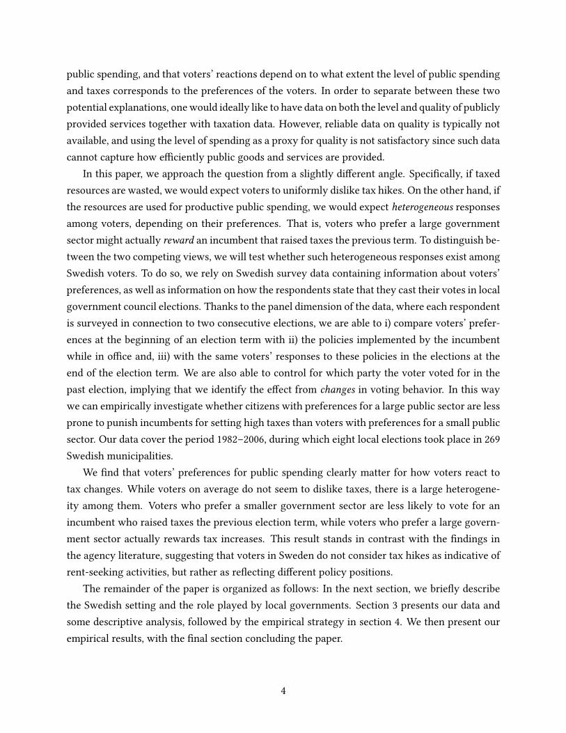
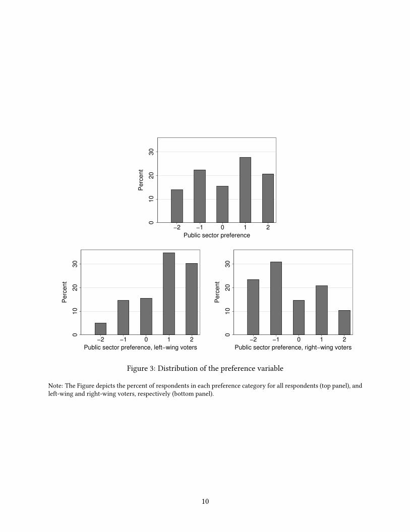
Figure 3 shows the shares for each response for the preference variable, where we code theresponses from -2 to 2 such that 2 is the most positive attitude towards the public sector. The �rstgraph is for the entire sample, while the second and third show the variable for left-wing votersand right-wing voters. As expected, left-wing voters are much more likely to have a positiveattitude towards public spending compared to right-wing voters.13

3.2 Municipality data

Out of Sweden’s 290 municipalities, we exclude the 21 municipalities that were involved in a splitor merger during the period of study. For the remaining 269 municipalities, we have aggregatedmunicipality data from Statistics Sweden on municipal tax rates, the number of seats held byeach party in the municipal council, as well as some other socioeconomic characteristics of themunicipalities.14

During the 1990s, there was a gradual transfer of responsibilities from the county to the mu-nicipal level, primarily concerning elderly care, which was combined with an increase in themunicipal tax rate and a corresponding decrease in the county tax rate. Because the total localtax rate (municipal + county tax rates) remained unchanged, we �nd it unlikely that voters wouldreact to changes in the municipal tax rate that occurred only because of the reform. We thereforeremove these tax changes in the data. In the appendix we describe these reform changes in moredetail and how we adjust the data.

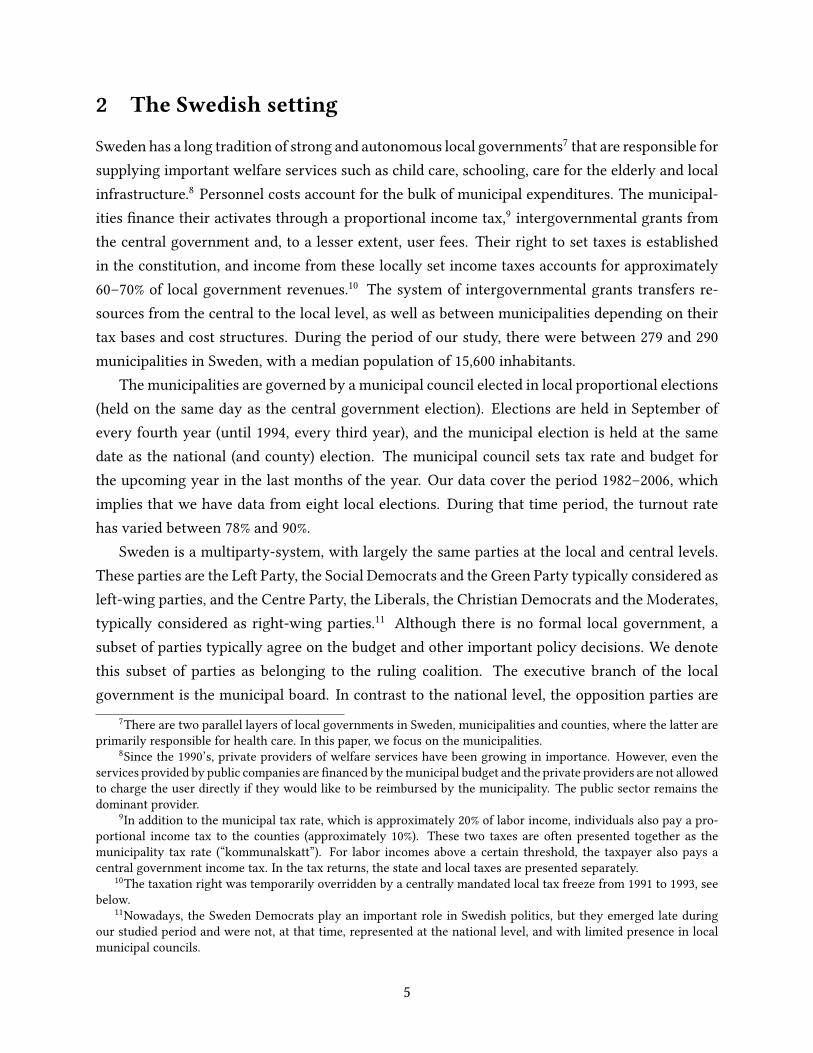
Figure 4 depicts the evolution of the municipal tax rate (after our adjustments). Between1982 and 2006, the municipal tax rate increased, on average, with around one percentage point.15

Consistent with the overall increase in the municipal tax rate, the graph also shows that in mostyears more municipalities increased than decreased the tax rate.

There is also a number of years where no municipality increased the tax rate. Between 1991–1993 there was a nationally mandated tax freeze where the municipalities were not allowed to

13It is not obvious how one should treat individuals responding “Neither a bad nor a good proposal”. In theempirical analysis, we interpret their responses as being satis�ed with the current level of public consumption (andtaxes). Alternatively, we could consider these individuals as being indi�erent between a large and small public sector.If these individuals are excluded, the main �nding of the paper is unchanged (results available upon request).

14We use, among other variables, unemployment rate as a control variable. That variable comes from the Swedishunemployment agency, Arbetsförmedlingen.

15The county tax was included in the municipal tax for the municipalities of Gotland (whole time period), Göte-borg and Malmö (until the year 1998).

9

010

20

30

Perc

ent

−2 −1 0 1 2

Public sector preference

010

20

30

Perc

ent

−2 −1 0 1 2

Public sector preference, left−wing voters

010

20

30

Perc

ent

−2 −1 0 1 2

Public sector preference, right−wing voters

Figure 3: Distribution of the preference variable

Note: The Figure depicts the percent of respondents in each preference category for all respondents (top panel), andleft-wing and right-wing voters, respectively (bottom panel).

10

increase the local tax rate above the 1990 level. In addition, for the years 1994, 1997 and 1998, thecentral government incentivized municipalities with intergovernmental grants to not raise taxes,something that had a very similar e�ect as the tax freeze (see Statskontoret 2011). In a sensitivityanalysis below, we address this particular issue.

3.3 Coalition data

Our third set of data concerns coalitions at the local level. Previous literature analyzing Swedishpolitics has tended to classify the parties into belonging to a left-wing and right-wing bloc (see,e.g., Alesina et al. 1997, Pettersson-Lidbom 2008). In this paper we use data on actual coalitions.For the last three elections terms (1994–2006) such data is available from SKL (Swedish Associ-ation of Local Authorities and Regions). The data contain information on who formed a part ofthe ruling coalition after the election, and before the next election. In the analysis, we excludemunicipalities where the coalition changed during the election period. For the previous fourelection periods (between 1982–1994), we �elded our own survey to all Swedish municipalitieswhere we asked which parties formed ruling coalitions during the election period. In total, wereceived responses from 208 of the 269 municipalities in our sample (77% response rate). For dataon which party the chairman of the municipal board comes from, we have acquired the database“Kommunfakta” which contains this information. As can be seen from Figure 2, coalitions do notalways follow the traditional left-right dimension.

4 Empirical Strategy

In this paper, we are interested in testing whether voters’ reaction to tax changes depend on theirpreferences for public consumption. More speci�cally, is it the case that voters that prefer a largepublic sector are more inclined to reelect the incumbent local government if it has increased taxesduring its term in o�ce, than voters that prefer a smaller public sector? To answer this question,we estimate the following model:

vote_incijt = γt + β1∆taxjt + β2prefijt−1 + β3 (∆taxjt × prefijt−1)

+ ∆Zjtρ + ∆Zjt × prefijt−1δ + β4vote_incijt−1 + εijt, (1)

where the outcome variable, vote_incijt, is a dummy variable indicating whether the respondenti in municipality j at time t voted for one of the parties in the ruling coalition. Because oneway for citizens to show their discontent with their ruling politicians is to abstain from votingwe include also citizens who either abstained from voting, or who cast a blank vote. prefijt−1

11

16

16.5

17

17.5

0.2

5.5

1985 1990 1995 2000 2005year

Raised municipal tax Lowered municipal tax

Municipal tax

Figure 4: Evolution of municipal tax rate

Note: The Figure depicts the evolution of the municipal tax rate over time, excluding reform e�ects (the relevanty-axis is on the right-hand side). The bars show the share of municipalities that lowered and raised taxes during eachyear after reform e�ects have been removed (the relevant y-axis is on the left-hand side). The vertical lines indicateelection years.

12

is respondent i’s (living in municipality j) preference regarding the public sector reported atthe time of the previous election. This variable takes values from -2 to 2, where 2 indicatesa preference for a relatively larger public sector. ∆taxjt denotes the change in the municipalincome tax rate from the previous election. The variable of interest is the interaction betweenprefijt−1 and ∆taxjt. Our hypothesis is that there is a positive interaction e�ect between thesetwo variables (β3 > 0), indicating that voters who prefer a large public sector are relatively morelikely to vote for incumbents who raised taxes compared to voters who prefer a smaller publicsector. We also include time-speci�c intercepts, γt.

Important for our application is that prefijt−1 is determined before ∆taxjt which means thatwe can study voters’ reactions to tax changes depending on their preferences for the size of thepublic sector before the tax changes are realized. It is of course possible that taxes change duringthe election term in response to changing economic circumstances, not realized at the time of theprevious election. For instance, a negative shock to the economy, lowering the taxable income,might necessitate the municipalities to raise taxes to maintain public services. To control forsuch changing circumstances, not known by voters at time t − 1, we include a vector of time-varying municipal covariates in the vector ∆Zjt, which measure changes since last election. Thisvector includes controls that are likely to a�ect the municipal tax rate: changes in taxable income,unemployment rate, population size and share of young (aged 0 to 14) and old (aged 80 andabove). Because ∆taxjt is included both by itself, as well as interacted with prefijt−1, ∆Zjt mustbe included in the same way to �exibly control for changes in ∆taxjt due to changing economiccircumstances.

Finally, we also control for whether the respondent voted for the current incumbent in theprevious election, vote_incijt−1. By doing this, we control for voting preferences which are �xedover time, and instead estimate changes in voting behavior depending on how taxes changedduring the election term.

5 Results

5.1 Baseline estimates

We begin our empirical analysis by replicating the �nding from previous literature that voters,on average, are less likely to vote for incumbents who raise taxes. The �rst column in Table 1shows that an increase in the municipal tax rate with one percentage point is associated witha decrease in the probability of voting for the incumbent with approximately two percentagepoints. However, this e�ect is not statistically di�erent from zero. There is therefore only weak

13

evidence of voters on average disliking taxes.16

In the second column, we estimate the interaction model. Here we �nd a large positive, sta-tistically signi�cant, interaction e�ect between tax changes and voter preferences, in line withour hypothesis. Once municipality controls are included (column 3), the point estimate dropssomewhat but is still statistically signi�cant. In the fourth column we include the control for pastvoting behavior to estimate the baseline model (Equation 1). The point estimate drops further,but continues to be statistically signi�cant. As expected, the inclusion of past voting behaviorremoves much of the variation in the outcome variable, something that can be seen in the jumpin R2.

To get a sense of whether the estimated e�ect is large or small, it helps to relate it to changesin the tax rate. Our estimate indicates that an increase (decrease) in the municipal tax rate withone percentage point is associated with a relative increase (decrease) in the probability of votingfor the incumbent of around 15 percentage points for the voters most positive, compared to thoseleast positive, towards the public sector.17. This sounds like a very large e�ect, but note that aone percentage point change in the municipal tax rate is a large change; a change of at least thatmagnitude is observed in around 8% of the data. The corresponding number for a standard devi-ation change in the municipal tax rate is more than 6 percentage points. Because the preferencevariable is scaled between -2 and 2, the nonsigni�cant main e�ect of a change in the local taxrate implies that individuals who think it is neither a bad nor a good proposal to reduce the sizeof the public sector do not react to tax changes.

In the baseline speci�cation we do not include any individual level controls. The reason forthis omission is that, as opposed to municipality controls, it is not clear what type of endogeneityproblem individual controls solve. Nevertheless, in column 5 we show that the inclusion of indi-vidual controls for education, work status, age, gender, cohabiting status and presence of childrenin the home do not a�ect the result in any signi�cant way. Because there is no clear theoreticalreason for the individual controls we do not include them in the rest of the paper.

In the model in equation (1) there is a linear interaction between a tax change and public sectorpreference. With this approximation, the point estimate implies that there is a linear change inprobability of voting for the incumbent to a tax change depending on preferences. In Figure5 we show point estimates and con�dence intervals when vote_incijt has been regressed on∆taxjt (and year e�ects, municipal controls and voting for incumbent in last election) for eachpreference category separately. As comparison, the estimated marginal e�ect from the baselinemodel (column 4 of Table 1) is also included.

The �gure illustrates that it is the voters who are at the extremes of the preference distribution16Adding municipal controls do not make any di�erence for the results.170.037× (2− (−2)) ≈ 0.15

14

Table 1: Voting for incumbent coalition

(1) (2) (3) (4) (5)∆ Tax -0.020 -0.018 -0.016 -0.019 -0.019

(0.019) (0.020) (0.022) (0.018) (0.018)Pref., t− 1 0.025∗∗∗ 0.067∗∗∗ 0.0031 0.0095

(0.0085) (0.016) (0.011) (0.011)∆ Tax × Pref., t− 1 0.059∗∗∗ 0.045∗∗∗ 0.037∗∗∗ 0.036∗∗∗

(0.014) (0.015) (0.011) (0.010)Voted inc., t− 1 0.64∗∗∗ 0.64∗∗∗

(0.013) (0.013)Year e�ects X X X X X

Municipality controls X X X

Individual controls X

Obs. 4,749 4,749 4,749 4,581 4,392R2 0.00 0.02 0.02 0.43 0.45

Note: The dependent variable is an indicator for voting for any party in the incumbent coalition. The munic-ipality controls are included both by themselves, as well as interacted with the preference variable. Standarderrors, shown in parentheses, are clustered at the municipal level. ∗ p < 0.1, ∗∗ p < 0.05, ∗∗∗ p < 0.01.

that react to tax changes. The probability that voters think it is a very good proposal to reducethe size of the public sector is reduced with almost 11 (more than 4) percentage points for a onepercentage point (standard deviation) increase in the tax rate. Conversely for voters that are mostpositive towards the public sector a one percentage point (standard deviation) increase in taxesis associated with a 9 (almost 4) percentage points increase is support for the incumbent. Thepoint estimates are not statistically signi�cantly di�erent from zero for any of the three middlecategories.

5.2 Sensitivity analysis

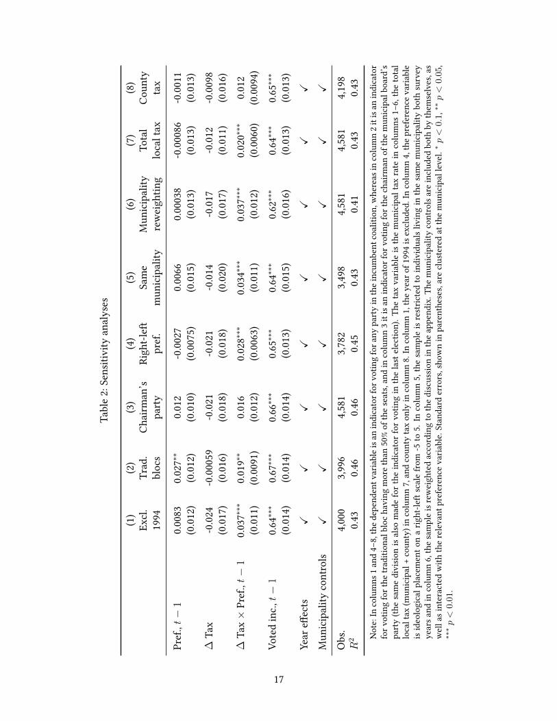
We now turn to testing the sensitivity of our results. As illustrated in Figure 4, during the years1991–1994 and 1997–1998, the municipalities could not freely increase that municipal tax rate,either because of a tax freeze or because of the central government grant system. In the �rstcolumn of Table 2 we therefore exclude the election period of 1991–1994, because this is the onlyelection period when municipalities could not raise taxes at all. The results are not a�ected inany way by this restriction.18

18If all election periods where the restriction was in place during at least part of the period (i.e., 1988–1998) areremoved, the interaction e�ect is even stronger. That result is available upon request.

15

−.2

−.1

0.1

.2

−2 −1 0 1 2

Figure 5: E�ect of change in municipal tax rate, by preference category

Note: Each of the �ve preference categories is shown on the x-axis. The �gure show the point estimates and 95%con�dence intervals for the estimated e�ect of a tax change on voting for the incumbent coalition for each preferencecategory separately. Standard errors are clustered at the municipal level. Municipal controls, year e�ects and controlfor voting for current incumbent in last election are included for each regression. The regression line show themarginal e�ect of a tax change from the estimation in column 4 of Table 1.

16

Tabl

e2:

Sens

itivi

tyan

alys

es

(1)

(2)

(3)

(4)

(5)

(6)

(7)

(8)

Excl

.Tr

ad.

Chai

rman

’sRi

ght-l

eft

Sam

eM

unic

ipal

ityTo

tal

Coun

ty19

94bl

ocs

party

pref

.m

unic

ipal

ityre

wei

ghtin

glo

calt

axta

x

Pref

.,t−

10.0

083

0.027

∗∗0.0

12-0

.0027

0.006

60.0

0038

-0.00

086

-0.00

11(0

.012)

(0.01

2)(0

.010)

(0.00

75)

(0.01

5)(0

.013)

(0.01

3)(0

.013)

∆Ta

x-0

.024

-0.00

059

-0.02

1-0

.021

-0.01

4-0

.017

-0.01

2-0

.0098

(0.01

7)(0

.016)

(0.01

8)(0

.018)

(0.02

0)(0

.017)

(0.01

1)(0

.016)

∆Ta

x×

Pref

.,t−

10.0

37∗∗

∗0.0

19∗∗

0.016

0.028

∗∗∗

0.034

∗∗∗

0.037

∗∗∗

0.020

∗∗∗

0.012

(0.01

1)(0

.0091

)(0

.012)

(0.00

63)

(0.01

1)(0

.012)

(0.00

60)

(0.00

94)

Vote

din

c.,t−

10.6

4∗∗∗

0.67∗

∗∗0.6

6∗∗∗

0.65∗

∗∗0.6

4∗∗∗

0.62∗

∗∗0.6

4∗∗∗

0.65∗

∗∗

(0.01

4)(0

.014)

(0.01

4)(0

.013)

(0.01

5)(0

.016)

(0.01

3)(0

.013)

Year

e�ec

tsX

XX

XX

XX

X

Mun

icip

ality

cont

rols

XX

XX

XX

XX

Obs

.4,0

003,9

964,5

813,7

823,4

984,5

814,5

814,1

98R

20.4

30.4

60.4

60.4

50.4

30.4

10.4

30.4

3N

ote:

Inco

lum

ns1a

nd4–

8,th

edep

ende

ntva

riabl

eisa

nin

dica

torf

orvo

ting

fora

nypa

rtyin

thei

ncum

bent

coal

ition

,whe

reas

inco

lum

n2i

tisa

nin

dica

tor

forv

otin

gfo

rthe

tradi

tiona

lblo

chav

ing

mor

eth

an50

%of

the

seat

s,an

din

colu

mn

3it

isan

indi

cato

rfor

votin

gfo

rthe

chai

rman

ofth

em

unic

ipal

boar

d’s

party

(the

sam

edi

visio

nis

also

mad

efo

rthe

indi

cato

rfor

votin

gin

the

last

elec

tion)

.The

tax

varia

ble

isth

em

unic

ipal

tax

rate

inco

lum

ns1–

6,th

eto

tal

loca

ltax

(mun

icip

al+

coun

ty)i

nco

lum

n7,

and

coun

tyta

xon

lyin

colu

mn

8.In

colu

mn

1,th

eyea

rof1

994

isex

clud

ed.I

nco

lum

n4,

thep

refe

renc

evar

iabl

eis

ideo

logi

calp

lace

men

ton

arig

ht-le

ftsc

ale

from

-5to

5.In

colu

mn

5,th

esa

mpl

eis

rest

ricte

dto

indi

vidu

alsl

ivin

gin

the

sam

em

unic

ipal

itybo

thsu

rvey

year

sand

inco

lum

n6,

thes

ampl

eisr

ewei

ghte

dac

cord

ing

toth

edisc

ussio

nin

thea

ppen

dix.

Them

unic

ipal

ityco

ntro

lsar

einc

lude

dbo

thby

them

selv

es,a

sw

ella

sint

erac

ted

with

the

rele

vant

pref

eren

ceva

riabl

e.St

anda

rder

rors

,sho

wn

inpa

rent

hese

s,ar

ecl

uste

red

atth

em

unic

ipal

leve

l.∗p<

0.1,

∗∗p<

0.05,

∗∗∗p<

0.01

.

17

It is possible that there are measurement error in the way we de�ne coalitions, especiallyfor the earlier period when we performed our own survey (1982–1994). We therefore considertwo alternatives to de�ning the incumbent. First, we de�ne the incumbent coalition by usingthe traditional way of dividing Swedish political parties into one left-wing and one right-wingbloc, where any municipality where neither bloc has a majority is excluded. Results in the secondcolumn indicate that with such a division, the point estimate decreases substantially, but is stillstatistically signi�cant at the 5% level. This decrease is consistent with the traditional blocs beingproxies for the real coalitions.

Second, we let the incumbent be de�ned as only the party the chairman of the board comesfrom (in the third column). The point estimate is less than half of the baseline estimate and notstatistically signi�cant. An interpretation of this result is that voters do not only hold the leadingparty accountable for tax policy, but also other parties in a ruling coalition.19

One possibility is that voters who prefer a small public sector do so because they believe thepublic sector works ine�ciently and that politicians are rent-seeking. In the fourth column wereplace the preference variable with respondents’ placement on a ideological scale, ranging from-5 (far to the right) to 5 (far to the left). While this variable might also be dependent on beliefsabout government e�ciency, it is likely less so than the public sector preference variable. We�nd the same pattern here with a positive and statistically signi�cant interaction e�ect. A onepercentage point increase (decrease) in the municipal tax rate is associated with a relative increase(decrease) on the probability of voting for the incumbent of more than 28 percentage points forthe voters most far to the left compared to those most far to the right. The corresponding numberfor a standard deviation change is almost 12 percentage points.

In the estimations so far, we have not put any restrictions in place that the respondents shouldlive in the same municipality during the election period to avoid selection bias in our results.Nonetheless, it is a possibility that individuals who recently moved in to a municipality are notaware of the tax changes during the election period. In column 5 we therefore restrict our sampleto respondents who lived in the same municipality at the time of both surveys. As shown in thetable, the results do not change much with this restriction.

In all our results, each individual has the same weight. An alternative would be to reweighthe sample according to the number of individuals entitled to vote in respectively municipality,to deal with possible selection bias in the survey at the municipal level. In column 6 we reweighthe sample in this way. As shown in the table, this reweighting does not a�ect the results in anysigni�cant way.20

19It should be noted that fewer individuals vote for the chairman’s party (32%), compared to any party in theruling coalition (46%), so in percentage term, the drop in point estimate is smaller.

20In the appendix we also show that the means of observable characteristics do not changes much when thesample is reweighted.

18

We focus on responses to the municipal tax because that is the tax that is set by the munici-pality. However, it is perhaps more likely that voters observe the total local tax (the municipalityand county tax) since those two taxes are often combined. Furthermore, by considering the totallocal tax, we do not have to take the reform e�ects into account since the reforms only implieddi�erences in responsibility between the municipality and county level. In column 7, we thereforeuse the total local tax instead of the municipal tax.

The point estimate of the interaction e�ect when using the total local tax is smaller in size,but also more precisely estimated. This decrease can mainly be explained by the standard de-viation of the total local tax being greater than the municipal tax (0.69 compared to 0.41). Astandard deviation increase (decrease) in the total local tax rate is associated with a relative in-crease (decrease) on the probability of voting for the incumbent of more than 5% for the votersmost positive, compared to those least positive, towards the public sector, an estimate very closeto the baseline estimate.21

Finally, in the eighth column, we only consider responses to the county tax. If voters are well-informed, we should not expect voters to hold the municipal coalition accountable for changesin the county tax. Indeed, while the estimate of the interaction e�ect is positive, it is smaller insize than the baseline estimate and not statistically signi�cant, suggesting that voters hold themunicipal coalition accountable for the municipal tax rate, but not the county tax rate.22

5.3 Heterogeneous e�ects

Finally, we perform a number of heterogeneity analyses in order to dig deeper into the mechanismat hand. First, if voters have low con�dence in politicians it would make more sense for themto interpret a tax increase as a signal of rent-seeking activities, rather than as being used forproductive public spending. Hence, we would expect the interaction e�ect to be less pronouncedfor individuals with lower trust in their elected o�cials if they believe taxes are wasted anyway.We therefore split the sample into two groups, one for individuals who have fairly high or veryhigh con�dence in politicians and the other for individuals who have fairly low or very low

21It should be noted that in all estimations in this paper, standard errors are clustered at the municipal level. Forthe estimations in the last two columns, the tax rate vary partly, or completely, at the county level. It therefore seemslikely that cluster e�ects exist at the county level. Indeed, if standard errors are clustered at the county level, thestandard errors increase somewhat for the last two columns (results are available upon request). However, becausethere are only 21 counties, the cluster-robust covariance matrix is unlikely to be correctly estimated. We thereforecluster at the municipal level, but note that the standard errors in the last two columns are likely lower-boundestimates.

22In terms of size of the point estimate, a standard deviation increase (decrease) in the county tax rate is associatedwith a relative increase (decrease) on the probability of voting for the incumbent of around 2.4% for the voters mostpositive, compared to those least positive, towards the public sector.

19

con�dence in politicians.23

Table 3: Voting for incumbent coalition

Con�dence Coalition seats Coalition type(1) (2) (3) (4) (5) (6) (7)

Low High Min. Maj. Left Right Other∆ Tax -0.014 -0.024 0.0093 -0.026 0.016 -0.047∗ -0.054

(0.025) (0.037) (0.028) (0.022) (0.020) (0.025) (0.050)Pref., t− 1 -0.019 -0.0045 0.046 -0.0037 0.036∗∗∗ -0.10∗∗∗ 0.00015

(0.020) (0.027) (0.030) (0.012) (0.014) (0.025) (0.037)∆ Tax × Pref., t− 1 0.069∗∗∗ 0.018 0.013 0.046∗∗∗ 0.0089 0.054∗∗∗ 0.067∗∗

(0.016) (0.021) (0.010) (0.014) (0.012) (0.018) (0.028)Voted inc., t− 1 0.56∗∗∗ 0.67∗∗∗ 0.67∗∗∗ 0.64∗∗∗ 0.63∗∗∗ 0.64∗∗∗ 0.57∗∗∗

(0.019) (0.022) (0.022) (0.015) (0.019) (0.025) (0.034)Year e�ects X X X X X X X

Municipality controls X X X X X X X

Obs. 1,939 1,341 912 3,669 2,468 1,174 939R2 0.33 0.48 0.47 0.42 0.47 0.48 0.35

Note: The dependent variable is an indicator for voting for any party in the incumbent coalition. The munic-ipality controls are included both by themselves, as well as interacted with the preference variable. Standarderrors, shown in parentheses, are clustered at the municipal level. ∗ p < 0.1, ∗∗ p < 0.05, ∗∗∗ p < 0.01.

The �rst two columns in Table 3 show the opposite pattern to what we expect. The interactione�ect is greater for individuals with low con�dence in politicians. One explanation for this isthat low-trust individuals are more mobile in terms of voting, something that can be seen by pastvoting behavior being a weaker predictor of current voting behavior.

In many instances, the incumbent coalition does not have a majority of the seats in the munic-ipal council, and can therefore not decide themselves on any tax changes. A question is thereforeif voters are less likely to hold minority coalitions accountable for tax changes compared to ma-jority coalitions. In columns 3 and 4, we split the sample according to whether the incumbentcoalition has a minority or majority of the seats in the council. The interaction e�ect is onlypositive and signi�cant for the latter, suggesting that voters are more likely to hold a majorityaccountable for tax policy.

Finally, we also split the sample according to whether the incumbent coalition consists onlyof left-wing or right-wing parties, or whether it consists of other coalitions. Here we �nd that

23The respondents were asked the following: “Generally speaking, how high is your con�dence in Swedish politi-cians? Is it very high, fairly high, fairly low or very low?” The question was asked from 1988 and onwards.

20

the interaction e�ect does not exist for left-wing coalitions, but that it exists for right-wing andother coalitions. It is not obvious why this di�erence exist. For the “other” coalitions, the dif-ference can partially be explained by them almost always being majority coalitions (93% in thesample, compared to 78% for left-wing coalitions). This explanation does not work for right-wingcoalitions however, where only 73% are majority coalitions. An interesting avenue for future re-search would be to explain these di�erences in reactions to tax policy depending on the politicalalignment of the coalition in power.

6 Concluding discussion

In this paper, we set out to reach an improved understanding for how voters think about taxes.Do they perceive taxes as going to sel�sh politicians to collect rents, or do voters see them as�nancing valuable welfare services? Our point of departure was the political-agency literaturewhere rational voters react to past policies in order to select good politicians or to disciplinebad politicians. By investigating whether voters’ responses to tax changes di�er depending ontheir preferences for public services, we claim to test whether voters use elections to punishrent-seeking behavior, or as a means to divide funds between public and private consumption.Di�erent from previous studies, we have therefore not focused on average responses in the elec-torate, but instead on the heterogeneity among voters.

Using survey data where voters are interviewed in two consecutive elections, together withadministrative data, we were able to estimate how Swedish voters react to changes in the localtax rate. We �nd that that voters who prefer a large government sector are indeed more likelyto react positively (negatively) to tax increases (decreases), compared to voters who prefer lessgovernment spending. This result is true even if we control for past voting behavior and alsorobust to a number of di�erent sensitivity checks.

If there is one group of voters where we might expect taxes as being seen as indicative of rent-seeking behavior, it would be for voters who have little con�dence in their elected politicians.Surprisingly, our �ndings do not lend support to this conjecture. In contrast, the reaction to taxchanges depend to a larger extent on the policy preferences for this group, compared to voterswith more con�dence in their politicians.

Our conclusion based on our results is therefore that voters do not consider tax hikes to be anindicator of bad incumbent behavior, as suggested in much of the rent-seeking literature. Instead,our �ndings suggest that responses to tax changes are more likely to follow citizens’ preferencesfor public spending. It should be noted, however, that it is far from clear to what extent thisresult would translate to di�erent institutional settings. Sweden is a country where support forgovernment intervention is comparatively high, and with low levels of corruption. An interesting

21

avenue for future research would therefore be whether heterogeneity among voters exist even inother institutional contexts.

References

Acemoglu, D., Egorov, G., and Sonin, K. (2013). A political theory of populism. Quarterly Journalof Economics, 128(2):771–805.

Alesina, A. and Cukierman, A. (1990). The politics of ambiguity. Quarterly Journal of Economics,105(4):829–850.

Alesina, A., Roubini, N., and Cohen, G. D. (1997). Political Cycles and the Macroeconomy. MITPress, Cambridge.

Alt, J., Bueno de Mesquita, E., and Rose, S. (2011). Disentangling accountability and competencein elections: Evidence from u.s. term limmits. The Journal of Politics, 73(1):171–186.

Andrikopoulus, A., Loizides, I., and Prodromidis, K. (2004). Fiscal policy and political businesscycles in the EU. European Journal of Political Economy, 20:125–152.

Barro, R. J. (1973). The control of politicians: An economic model. Public Choice, 14(1):19–42.

Besley, T. (2006). Principled Agents? The Political Economy of Good Government. Oxford UniversityPress, New York.

Besley, T. and Case, A. (1995a). Does electoral accountability a�ect economic policy choices?evidence from gubernatorial term limits. Quarterly Journal of Economics, 110(3):769–798.

Besley, T. and Case, A. (1995b). Incumbent behavior: Vote-seeking, tax-setting, and yardstickcompetition. American Economic Review, 85:25–45.

Besley, T. and Coate, S. (1997). An economic model of representative democracy. QuarterlyJournal of Economics, 112:85–114.

Bordignon, M., Cernigliac, F., and Revelli, F. (2004). Yardstick competition in intergovernmentalrelationships: Theory and empirical predictions. Economics Letters, 83(3):325–333.

Cukierman, A. and Tommasi, M. (1998). When does it take a Nixon to go to China? AmericanEconomic Review, 88(1):180–197.

Dahlberg, M. and Mörk, E. (2011). Is there an election cycle in public employment? separatingtime e�ects from election year e�ects. CESifo Economic Studies, 57(3):480–498.

22

Ferejohn, J. (1986). Incumbent performance and electoral control. Public choice, 50(1):5–25.

Folke, O. and Rickne, J. (2016). The glass ceiling in politics formalization and empirical tests.Comparative Political Studies, 49(5):567–599.

Foremny, D. and Riedel, N. (2014). Business taxes and the electoral cycle. Journal of PublicEconomics, 115:48–61.

Kneebone, R. D. and McKenzie, K. J. (2001). Electoral and partisan cycles in �scal policy: Anexamination of canadian provinces. International Tax and Public Finance, 8:753–774.

Lowry, R. C., Alt, J. E., and Ferree, K. E. (1998). Fiscal policy outcomes and electoral accountabilityin american states. American Political Science Review, 92(4):759–774.

Niemi, R. G., Stanley, H. W., and Vogel, R. J. (1995). State economies and state taxes: Do votershold governors accountable? American Journal of Political Science, 39(4):936–957.

Osborne, M. J. and Slivinsky, A. (1996). A model of political competition with citizen-candidate.Quarterly Journal of Economics, 111:65–96.

Peltzman, S. (1992). Voters as �scal conservatives. Quarterly Journal of Economics, 107(2):327–361.

Persson, T. and Tabellini, G. (2000). Political Economics: Explaining Economic Policy. MIT Press,Cambridge.

Pettersson-Lidbom, P. (2006). Testing political agency models. SSRN Scholarly Paper ID 988355.

Pettersson-Lidbom, P. (2008). Do parties matter for economic outcomes? a Regression-Discontinuity approach. Journal of the European Economic Association, 6(5):1037–1056.

Revelli, F. (2002). Local taxes, national politics and spatial interactions in english district electionresults. European Journal of Political Economy, 18:281–299.

Rogo�, K. (1990). Equilibrium political budget cycles. American Economic Review, 80(1):21–36.

Schultz, C. (2002). Policy biases with voters’ uncertainty about the economy and the government.European Economic Review, 46:487–506.

Statskontoret (2011). Kommunalt självstyre och proportionalitet. Statskontoret 2011:17.

23

Appendix

A Reforms

During the studied period, responsibilities were gradually transferred from the county level tothe municipal level for some welfare services, primarily elderly care. As a consequence of thereforms, the municipal tax rate increased, while the county tax rate decreased with the sameamount, leaving the total tax burden unchanged. These reforms took place at di�erent times indi�erent counties.24

In our data, we do not observe when these reforms took place, but we observe both changesto the municipal and county tax rates. For us to classify a tax change as due to a reform, twoconditions need to be ful�lled: (i) a majority of municipalities within a county and year in-creased/decreased taxes with the same amount, and (ii) the county tax rate went in the oppositedirection. The only exception to this rule is Blekinge län in 1996 where the �ve municipalities inthe county raised taxes with di�erent amounts: 1.74, 2.49, 2.64, 2.74 and 2.75 percentage points.Because the county tax rate was lowered with 1.74 at the same time, we consider the reform tobe 1.74. Table 4 shows the reforms for each county and election period.

24At a given point in time, a municipality belongs to one and only one county.

24

Table 4: Reform changes in municipal tax rate1

County 82–85 85–88 88–91 91–94 94–98 98–02Stockholms län 0 0 0 1.8 1.7 0.08Uppsala län 0 0 0 2.2 1.79 0.19Södermanlands län 0 0 0 2.67 1.3 0.31Östergötlands län 0.25 0 0 1.85 1.64 0.16Jönköpings län 0 0 0 2 1.64 0.19Kronobergs län 0 0 0 2.75 1.75 0.21Kalmar län 0 0 0 2.7 2.13 0.23Gotlands län2 0 0 0 0 0 0Blekinge län 0 0 0 1.95 1.74 0.1Kristianstads län 0 0 0 2.3 1.65 -Malmöhus län 0 0 0 2.27 1.34 -Skåne län - - - - - 3

Hallands län 0 0 1.5 2.05 0.25 0.23Göteborgs och Bohus län 0 0 0 3.77 0.19 -Älvsborgs län 0 0.4 0 2.85 1.46 -Skaraborgs län 0 0 0 2.7 1.37 -Västra Götalands län - - - - - 3

Värmlands län 0 0 0 3.05 1.75 0.2Örebro län 0 0 0 2.2 1.52 0.2Västmanlands län 0 0 0 2.9 1.6 0.19Dalarnas län 0 0 0 3.93 0.12 0.26Gävleborgs län 0 0 0 2 1.74 0.16Västernorrlands län 0 0 0 3.05 2 0.24Jämtlands län 0 0 0 2.55 2.38 0.14Västerbottens län 0 0 0 2.65 2.25 0Norrbottens län 0 0 0 3.35 1.37 0.06

1 No reforms occured 02–06.2 Gotlands län has been a municipality and county for the whole time period. It has therefore not been directly

a�ected by the reforms.3 In 1998, Kristianstads län and Malmöhus län merged into Skåne län whereas Göteborgs och Bohus län, Älvsborgs

län and Skaraborgs län merged into Västra Götalands län. The reform e�ect for the municipalities in the formerKristianstads län during the period 98–02 was 0.16 and for the municipalities in the former Malmöhus län was0.13. Similarly, for the counties that merged into Västra Götalands län, the reform e�ect was 0.43 (Göteborgsoch Bohus län), 0.18 (Älvsborgs län) and 0.22 (Skaraborgs län).

25

B Sampling

The Swedish National Election Study is a survey with high response rates. For the years weanalyze, the response rate varied between 69% and 82%. Nevertheless, because we require therespondents to be interviewed in two consecutive elections, the response rate in our sample islower. Furthermore, not all respondents answer all questions, and we also put restrictions onwhich municipalities are included in the sample. An important question is therefore to whatextent our sample is representative of Swedish citizens.

Figure 6 shows the attrition in the di�erent stages of the survey. In total, there were 13,305individuals which were randomly selected to be included in the sample for the �rst time during theelection surveys 1982–2002, and eligible for inclusion a second time in the next election (for ourstudied period 1985–2006). 77% of these answered the survey. However, they did not necessarilyanswer all questions in the survey because respondents who refused to answer the full surveyhad the opportunity to answer shortened versions. For the �rst survey wave, the question weare primarily interested in is the question of preference for public spending. In total, there were8,420 respondents who stated such a preference.

Out of these, we can match 81% to answers in the following election. The rest is missing,either because they did not answer the second survey, or because their ID number is missing(this is true for 456 observations of the 1988 survey). For the second survey, the question ofinterest is the vote decision. We are able to use data when either the respondents stated whothey voted for, or when registers showed that they did not vote. This restriction further reducesthe sample size to 6,464. Therefore, approximately half of the observations remain after all theserestrictions have been put in place. Unrelated to individual selection, we also exclude a number ofmunicipalities because they where part of a split or a merger during the studied period, becausethere was either an unclear majority situation, or because majorities shifted during the electionperiod. These considerations reduce the sample to the �nal size of 4,749, which is our baselinesample.

To analyze how this attrition a�ects the characteristics of the respondents, Table 5 showsmeans of a number of variables for di�erent samples. All characteristics are measured at thetime of the �rst survey. The �rst column shows data which are available from registers, thereforeincluding individuals who refused, or were unable, to take part in any survey. The second columnshows the means for individuals who answered the �rst survey, whereas column 3 shows the samefor our �nal baseline sample.

In column 4 we reweight the sample based on expected number of respondents per munici-pality. Let njt be the number of eligible voters in municipality j at election year t and n̂jt be the

26

number of respondents in our baseline sample. The weight we use is

wj =

∑t njt∑

j

∑t njt

/ ∑t n̂jt∑

j

∑t n̂jt

. (2)

That is, we increase (decrease) the weight for respondents from municipalities where fewer (more)respondents than expected were drawn. If the incidence of non-responses vary systematically bymunicipality, we might expect this reweighting to signi�cantly change the characteristics of therespondents.

The table illustrate how observable characteristics di�er between samples. Standard errors ofthe means are shown in parentheses. Given the large sample size, standard errors are generallyvery small.25 The most obvious di�erence is that non-respondents tend to vote to a lesser extentcompared to respondents. Here it should also be noted that the average turnout rate duringthe studied period was around 83%, meaning that even the original sample (Sample I) does notseem to be completely random. In general, the di�erences between those who answered the �rstsurvey (Sample II) and both (Sample III) are quite small. For the independent variable of interest(public sector preference), the di�erence is negligible. The reweighting based on expected numberof voters at the municipal level (column 4) does not seem to change observable characteristicsmuch. There is therefore no clear evidence of systematic sample selection at the municipal level.

25The sample size di�ers for the di�erent variables due to not all individuals answering all questions.

27

Sample I: Randomly selected tobe part of �rst wave, 1982–2002

(n = 13, 035)

Did not participate in �rstinterview (n = 2, 968)

Sample II: Took partin �rst wave interview

(n = 10, 067)

Did not answer preferencequestion (n = 1, 159)

Answered do not know / donot want to answer on pref-erence question (n = 488)

Stated a preferencefor public spending

(n = 8, 420)

Did not participate in secondinterview or ID informa-

tion is missing (n = 1, 564)

Took part in second waveinterview, 1985–2006, and

ID information is complete(n = 6, 856)

Vote information is unavailable(n = 392)

Vote information available(n = 6, 464)

Municipality doesnot belong in sample

(n = 1, 715)

Sample III: Municipal-ity belongs in sample

(n = 4, 749)

Figure 6: Flow chart of attrition

28

Table 5: Descriptive statistics of di�erent samples

(1) (2) (3) (4)Sample I Sample II Sample III Sample III

Voted in municipal election 0.87 0.90 0.93 0.93(0.0030) (0.0030) (0.0038) (0.0040)

Age 46.0 45.3 44.1 44.1(0.15) (0.17) (0.23) (0.24)

Female 0.50 0.49 0.47 0.47(0.0044) (0.0050) (0.0072) (0.0076)

Public sector pref. 0.18 0.19 0.20(0.015) (0.020) (0.020)

Education level 1 0.23 0.19 0.18(0.0044) (0.0058) (0.0055)

Education level 2 0.091 0.095 0.091(0.0030) (0.0043) (0.0043)

Education level 3 0.096 0.090 0.084(0.0031) (0.0042) (0.0042)

Education level 4 0.065 0.066 0.064(0.0026) (0.0036) (0.0037)

Education level 5 0.17 0.18 0.18(0.0039) (0.0056) (0.0060)

Education level 6 0.13 0.13 0.14(0.0035) (0.0050) (0.0054)

Education level 7 0.22 0.24 0.26(0.0043) (0.0063) (0.0069)

Cohabiting 0.68 0.71 0.70(0.0048) (0.0066) (0.0071)

Children living at home 0.36 0.38 0.37(0.0050) (0.0071) (0.0074)

Do not work 0.33 0.29 0.30(0.0048) (0.0066) (0.0070)

Work national public sector 0.076 0.083 0.081(0.0027) (0.0040) (0.0040)

Work local public sector 0.19 0.20 0.20

29

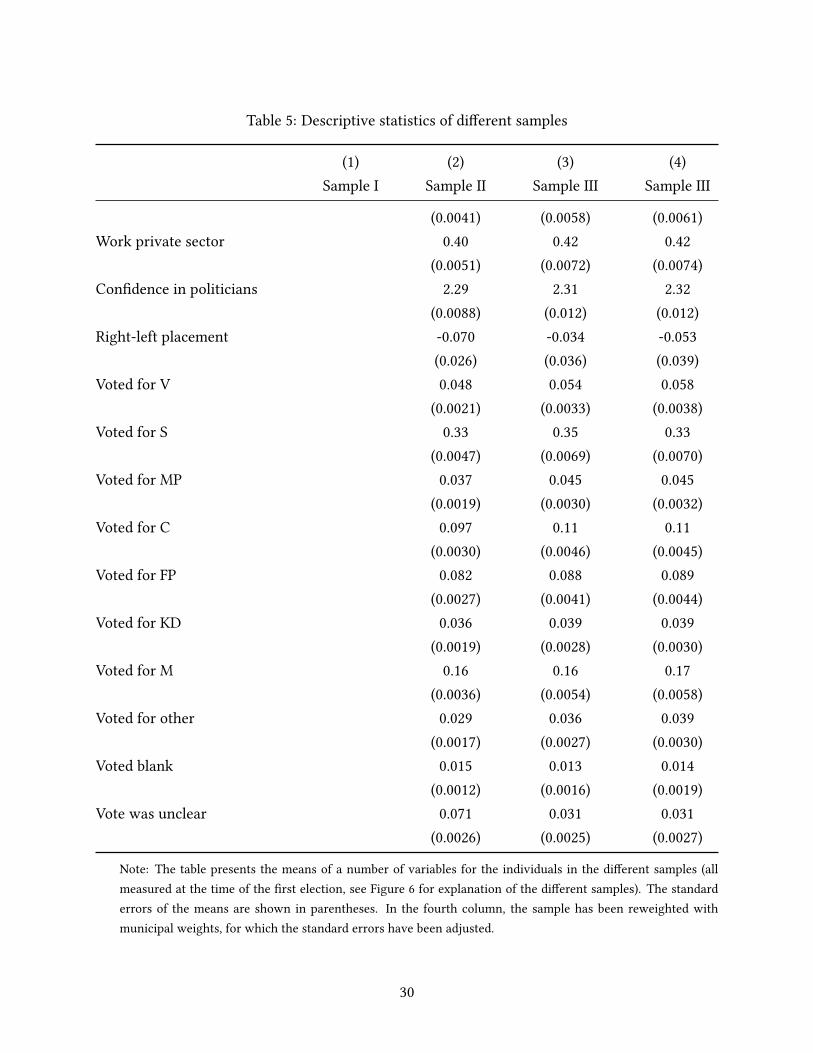
Table 5: Descriptive statistics of di�erent samples

(1) (2) (3) (4)Sample I Sample II Sample III Sample III

(0.0041) (0.0058) (0.0061)Work private sector 0.40 0.42 0.42

(0.0051) (0.0072) (0.0074)Con�dence in politicians 2.29 2.31 2.32

(0.0088) (0.012) (0.012)Right-left placement -0.070 -0.034 -0.053

(0.026) (0.036) (0.039)Voted for V 0.048 0.054 0.058

(0.0021) (0.0033) (0.0038)Voted for S 0.33 0.35 0.33

(0.0047) (0.0069) (0.0070)Voted for MP 0.037 0.045 0.045

(0.0019) (0.0030) (0.0032)Voted for C 0.097 0.11 0.11

(0.0030) (0.0046) (0.0045)Voted for FP 0.082 0.088 0.089

(0.0027) (0.0041) (0.0044)Voted for KD 0.036 0.039 0.039

(0.0019) (0.0028) (0.0030)Voted for M 0.16 0.16 0.17

(0.0036) (0.0054) (0.0058)Voted for other 0.029 0.036 0.039

(0.0017) (0.0027) (0.0030)Voted blank 0.015 0.013 0.014

(0.0012) (0.0016) (0.0019)Vote was unclear 0.071 0.031 0.031

(0.0026) (0.0025) (0.0027)

Note: The table presents the means of a number of variables for the individuals in the di�erent samples (allmeasured at the time of the �rst election, see Figure 6 for explanation of the di�erent samples). The standarderrors of the means are shown in parentheses. In the fourth column, the sample has been reweighted withmunicipal weights, for which the standard errors have been adjusted.

30