Revealed Preferences, Normative Preferences and

Behavioral Welfare Economics

David LaibsonHarvard University

January, 2010AEA Mini-course

Outline: • Normative preferences• Revealed preferences• Active decisions• Mechanism design example

Normative preferences• Normative preferences are preferences that society (or you)

should optimize• Normative preferences are philosophical constructs.• Normative debates can’t be settled with only empirical

evidence.

Positive Preferences(aka Revealed Preferences)

• Positive preferences are preferences that predict my choices

• Positive preferences need not coincide with normative preferences.

• What I do and what I should do are potentially different things (though they do have some connections).

• Equivalence between normative preferences and positive preferences is a philosophical position (for a nice defense of this view, see Bernheim and Rangel 2009).

An example:

32

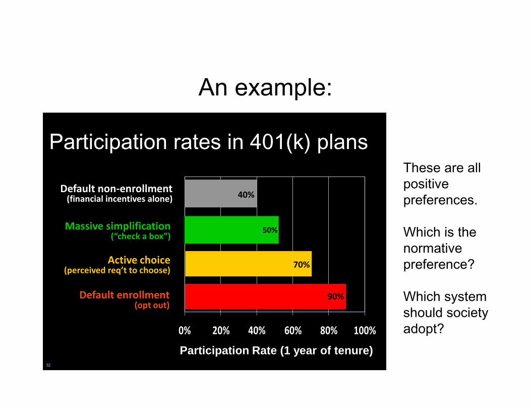
Improving participation in 401K plans(for a typical firm)

0% 20% 40% 60% 80% 100%

Default non‐enrollment(financial incentives alone) 40%

Massive simplification(“check a box”)

50%

Active choice(perceived req’t to choose)

70%

Default enrollment(opt out)

90%

Participation Rate (1 year of tenure)

These are all positive preferences.

Which is the normative preference?

Participation rates in 401(k) plans

Active decisionsCarroll, Choi, Laibson, Madrian, Metrick (2009)

Active decision mechanisms require employees to make an active choice about 401(k) participation.

• Welcome to the company• You are required to submit this form within 30 days of

hire, regardless of your 401(k) participation choice• If you don’t want to participate, indicate that decision • If you want to participate, indicate your contribution rate

and asset allocation• Being passive is not an option

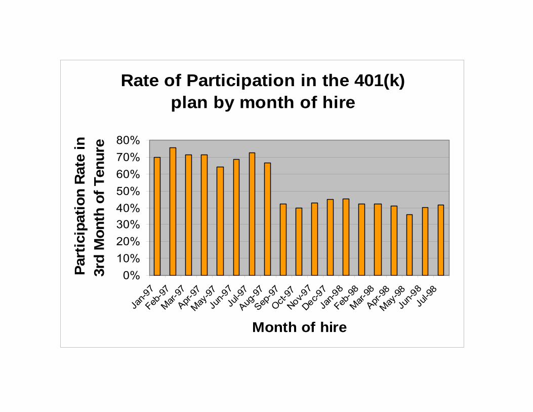
Rate of Participation in the 401(k) plan by month of hire

0%10%20%30%40%50%60%70%80%

Jan-9

7Feb

-97

Mar-97

Apr-97

May-97

Jun-9

7Ju

l-97

Aug-9

7Sep

-97

Oct-97

Nov-97

Dec-97

Jan-9

8Feb

-98

Mar-98

Apr-98

May-98

Jun-9

8Ju

l-98

Month of hire

Part

icip

atio

n R

ate

in

3rd

Mon

th o

f Ten

ure

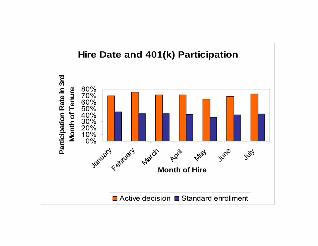
Hire Date and 401(k) Participation

0%10%20%30%40%50%60%70%80%

Janu

aryFeb

ruary

March

April

May

June July

Month of Hire

Parti

cipa

tion

Rat

e in

3rd

M

onth

of T

enur

e

Active decision Standard enrollment

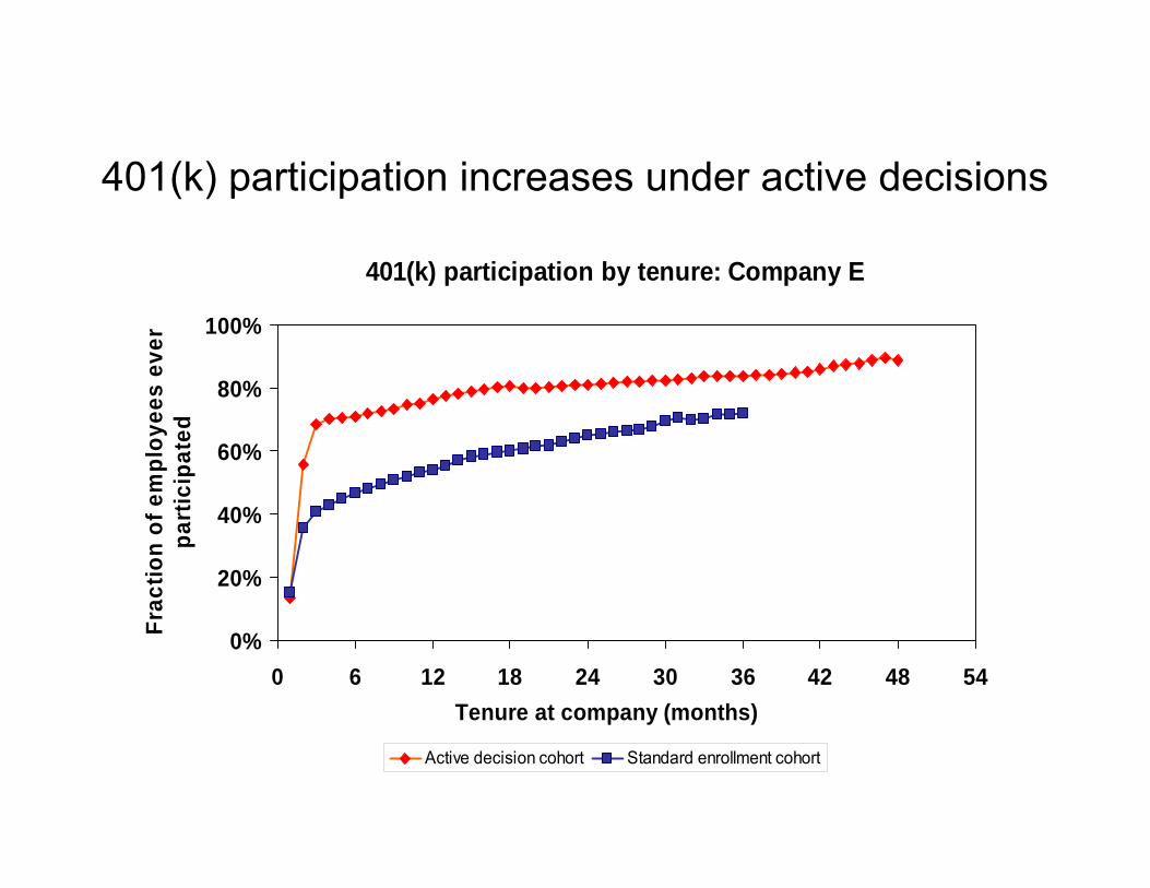
401(k) participation increases under active decisions

401(k) participation by tenure: Company E

0%

20%

40%

60%

80%

100%

0 6 12 18 24 30 36 42 48 54Tenure at company (months)

Frac

tion

of e

mpl

oyee

s ev

er

part

icip

ated

Active decision cohort Standard enrollment cohort

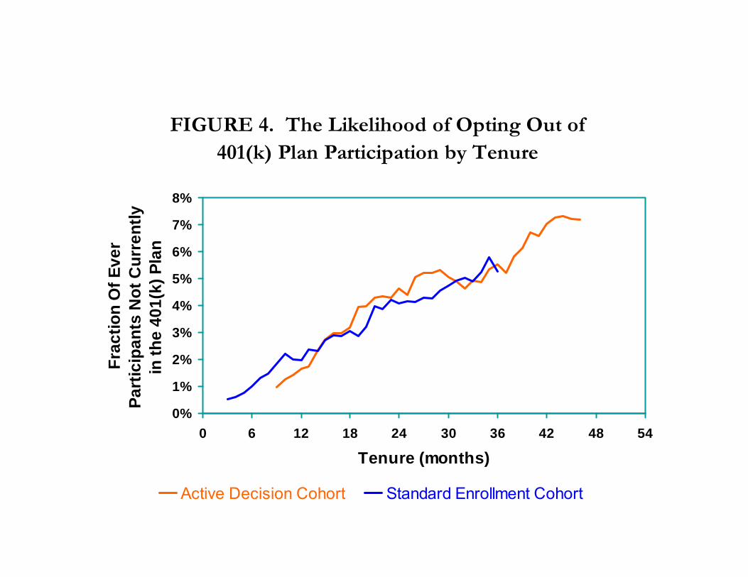
FIGURE 4. The Likelihood of Opting Out of 401(k) Plan Participation by Tenure

0%

1%

2%

3%

4%

5%

6%

7%

8%

0 6 12 18 24 30 36 42 48 54

Tenure (months)

Frac

tion

Of E

ver

Part

icip

ants

Not

Cur

rent

ly

in th

e 40

1(k)

Pla

n

Active Decision Cohort Standard Enrollment Cohort

Active decisions• Active decision raises 401(k) participation.

• Active decision raises average savings rate by 50 percent.

• Active decision doesn’t induce choice clustering.

• Under active decision, employees choose savings rates that they otherwise would have taken three years to achieve. (Average level as well as the entire multivariate covariance structure.)

An example:

32

Improving participation in 401K plans(for a typical firm)

0% 20% 40% 60% 80% 100%

Default non‐enrollment(financial incentives alone) 40%

Massive simplification(“check a box”)

50%

Active choice(perceived req’t to choose)

70%

Default enrollment(opt out)

90%

Participation Rate (1 year of tenure)

These are all positive preferences.

Which is the normative preference?

Which system should society adopt?

Participation rates in 401(k) plans

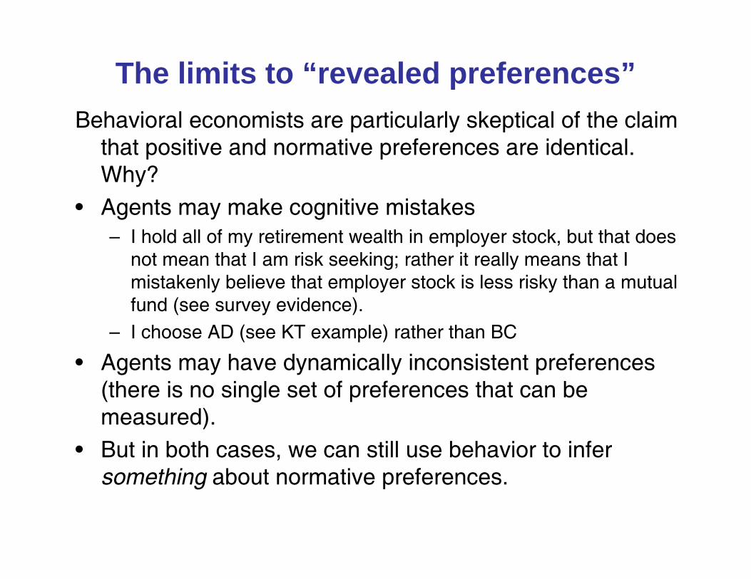
The limits to “revealed preferences”Behavioral economists are particularly skeptical of the claim

that positive and normative preferences are identical. Why?

• Agents may make cognitive mistakes– I hold all of my retirement wealth in employer stock, but that does

not mean that I am risk seeking; rather it really means that I mistakenly believe that employer stock is less risky than a mutual fund (see survey evidence).

– I choose AD (see KT example) rather than BC

• Agents may have dynamically inconsistent preferences (there is no single set of preferences that can be measured).

• But in both cases, we can still use behavior to infer something about normative preferences.

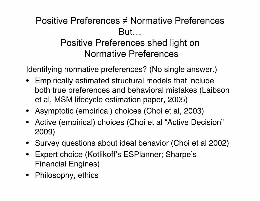
Positive Preferences ≠ Normative PreferencesBut…

Positive Preferences shed light onNormative Preferences

Identifying normative preferences? (No single answer.)• Empirically estimated structural models that include

both true preferences and behavioral mistakes (Laibson et al, MSM lifecycle estimation paper, 2005)

• Asymptotic (empirical) choices (Choi et al, 2003)• Active (empirical) choices (Choi et al “Active Decision”

2009)• Survey questions about ideal behavior (Choi et al 2002)• Expert choice (Kotlikoff’s ESPlanner; Sharpe’s

Financial Engines)• Philosophy, ethics

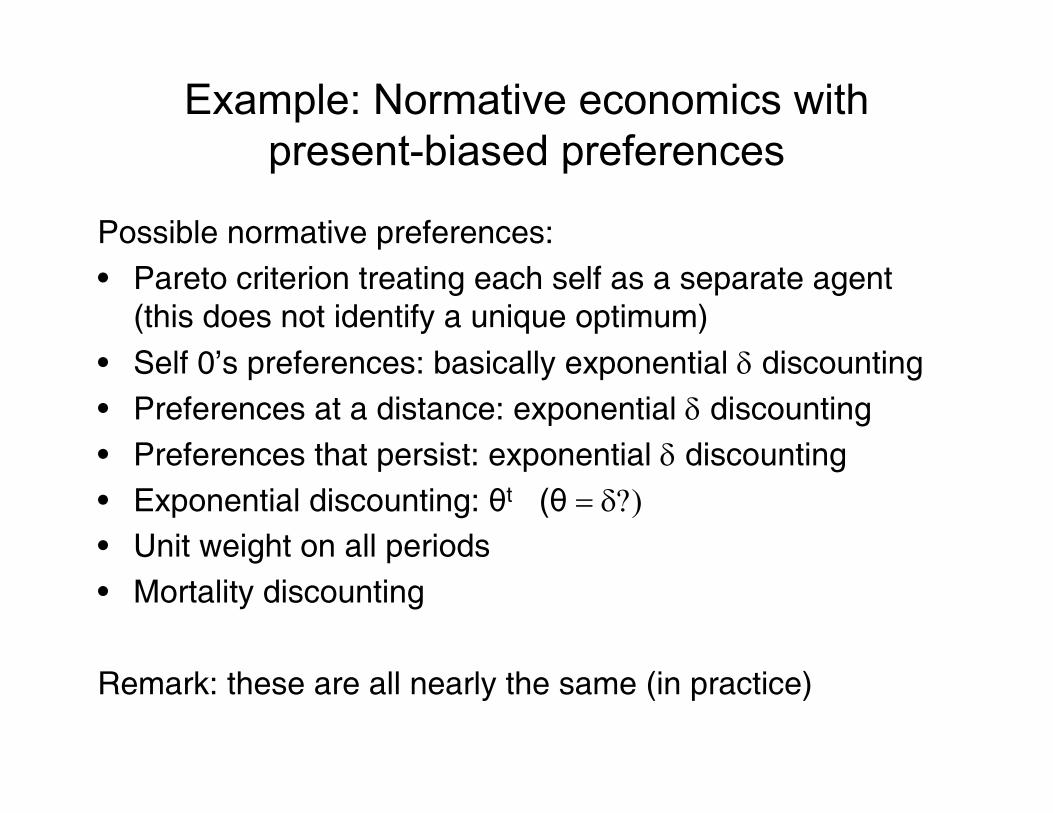
Example: Normative economics with present-biased preferences

Possible normative preferences:• Pareto criterion treating each self as a separate agent

(this does not identify a unique optimum)

• Self 0’s preferences: basically exponential δ discounting• Preferences at a distance: exponential δ discounting• Preferences that persist: exponential δ discounting• Exponential discounting: θt (θ = δ?)• Unit weight on all periods • Mortality discounting

Remark: these are all nearly the same (in practice)

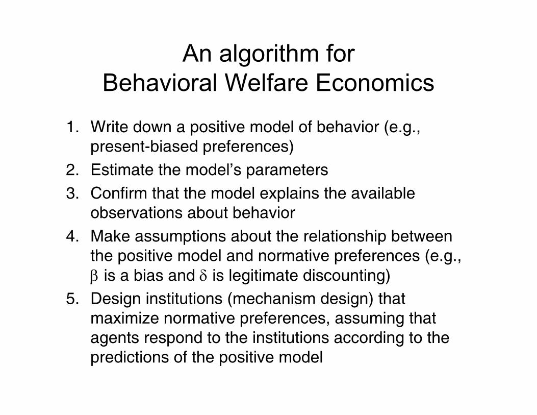
An algorithm for Behavioral Welfare Economics

1. Write down a positive model of behavior (e.g., present-biased preferences)

2. Estimate the model’s parameters3. Confirm that the model explains the available

observations about behavior4. Make assumptions about the relationship between

the positive model and normative preferences (e.g., β is a bias and δ is legitimate discounting)

5. Design institutions (mechanism design) that maximize normative preferences, assuming that agents respond to the institutions according to the predictions of the positive model

Some examples• Asymmetric/cautious paternalism (Camerer et al 2003) • Optimal Defaults (Choi et al 2003)• Libertarian paternalism (Sunstein and Thaler 2005)• Nudge (Sunstein and Thaler 2008)• Active Decisions and Optimal Defaults (Carroll et al 2009)

Optimal policies for procrastinatorsCarroll, Choi, Laibson, Madrian and Metrick (2009).

• It is costly to opt out of a default• Opportunity cost (transaction costs) are time-varying

– Creates option value for waiting to opt out• Actors may be present-biased

– Creates tendency to procrastinate

Preview of model

• Individual decision problem (game theoretic)

• Socially optimal mechanism design (enrollment regime)

• Active decision regime is optimal when consumers are:

– Well-informed

– Present-biased

– Heterogeneous

• Otherwise, defaults are optimal

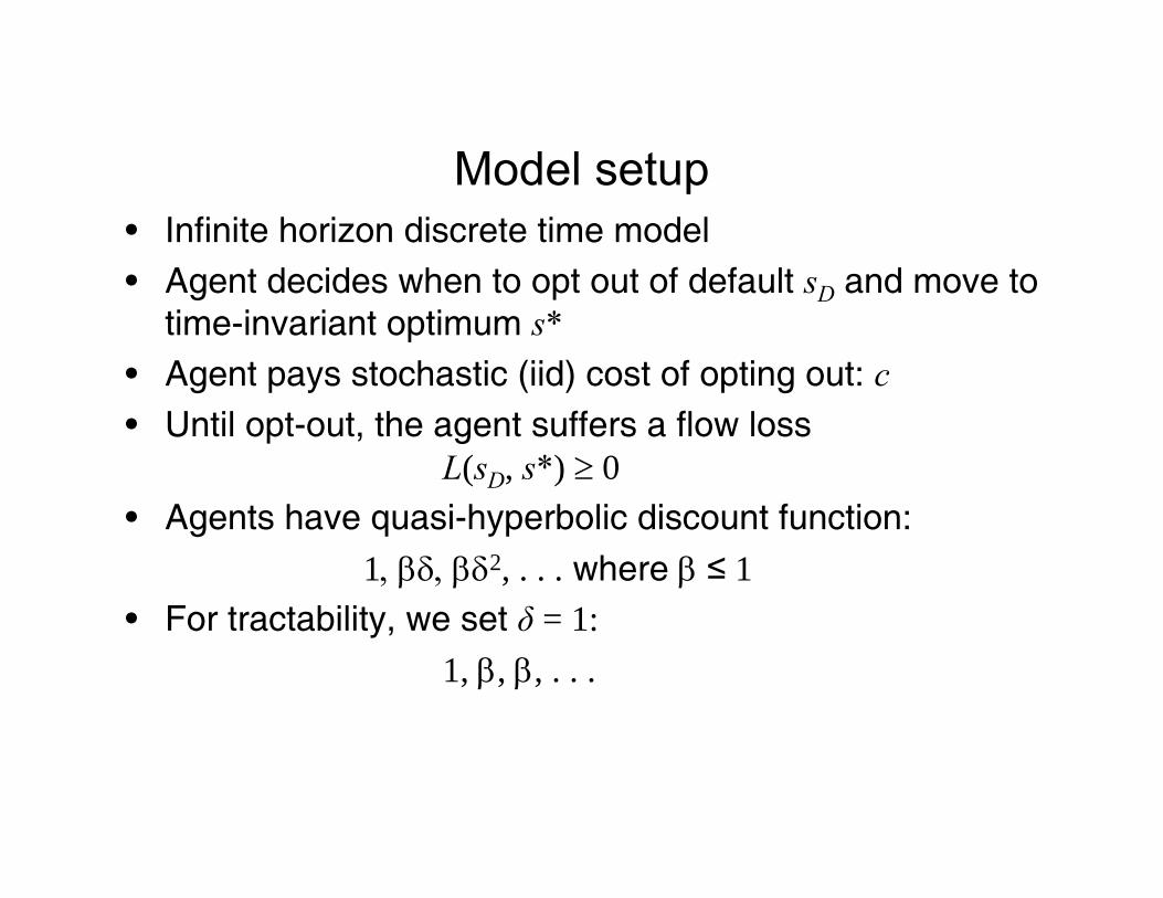
Model setup• Infinite horizon discrete time model• Agent decides when to opt out of default sD and move to

time-invariant optimum s*• Agent pays stochastic (iid) cost of opting out: c• Until opt-out, the agent suffers a flow loss

L(sD, s*) ≥ 0• Agents have quasi-hyperbolic discount function:

1, βδ, βδ2, . . . where β ≤ 1• For tractability, we set δ = 1:

1, β, β, . . .

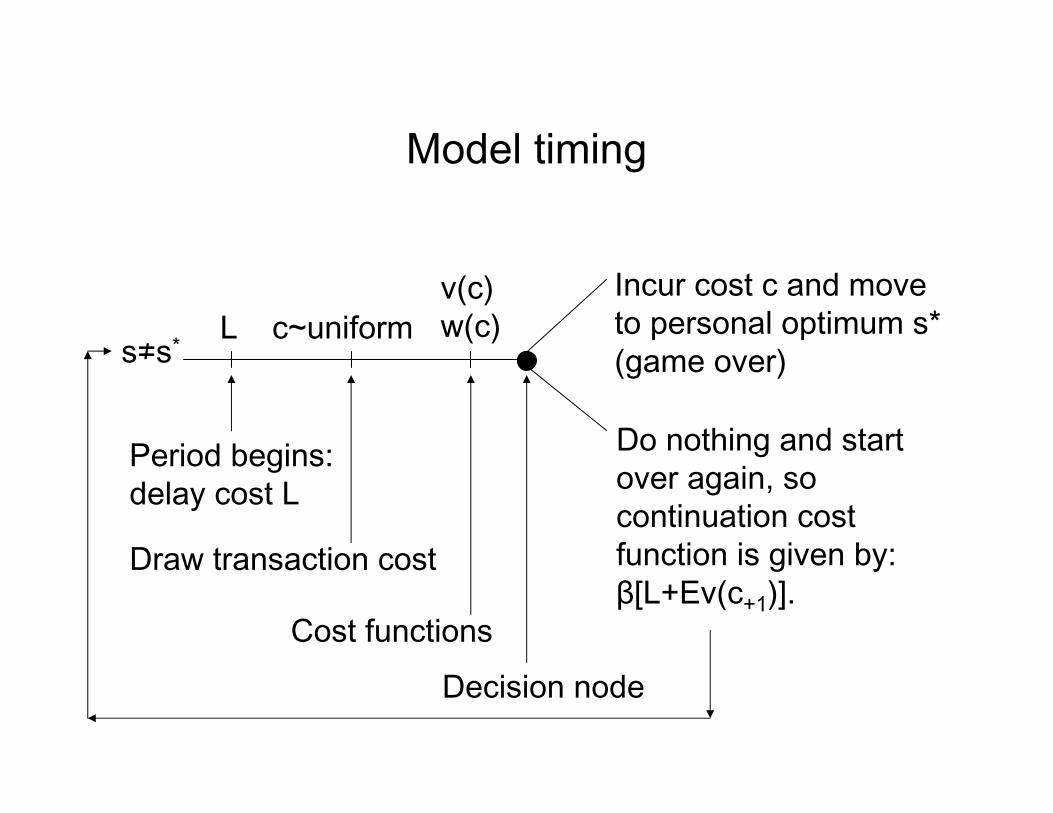
Model timing

s≠s* L c~uniformIncur cost c and moveto personal optimum s* (game over)

Do nothing and startover again, so continuation cost function is given by:β[L+Ev(c+1)].

v(c)w(c)

Period begins: delay cost L

Draw transaction cost

Decision nodeCost functions

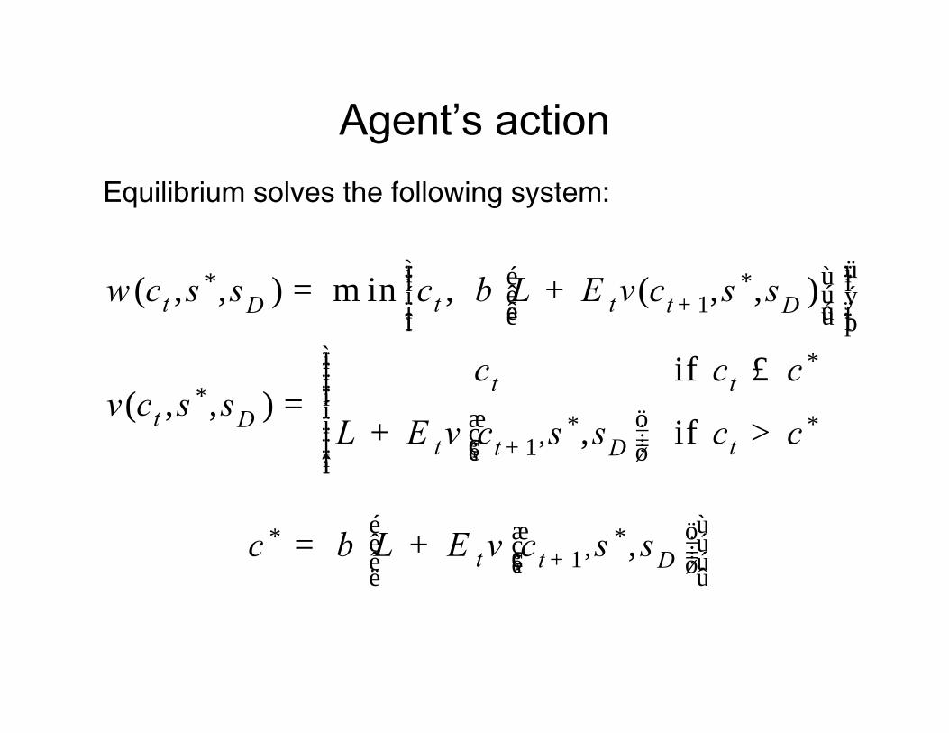
Agent’s actionEquilibrium solves the following system:

* *1

**

* *1,

( , , ) m in , ( , , )

if ( , , )

, if

t t t tD D

t tt D

t tt D

w c s s c L E v c s s

c c cv c s s

L E v c s s c c

b +

+

ì üï ïé ùï ïê úí ýï ïê úë ûï ïî þìïïïïïí æ öï ÷çï ÷ç ÷çï è øïïî

= +

£=

+ >

* *1, ,t t Dc L E v c s sb +

é ùæ öê ú÷ç ÷ç ÷çê úè øë û= +

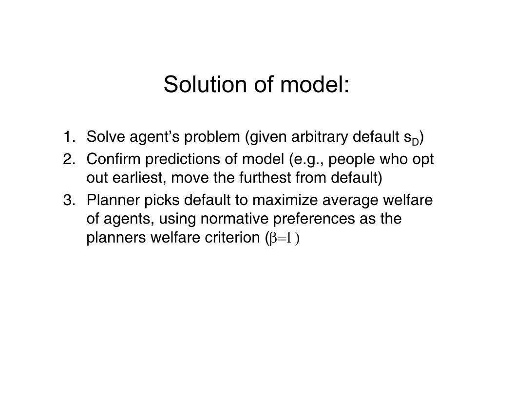
Solution of model:

1. Solve agent’s problem (given arbitrary default sD)2. Confirm predictions of model (e.g., people who opt

out earliest, move the furthest from default)3. Planner picks default to maximize average welfare

of agents, using normative preferences as the planners welfare criterion (β=1)

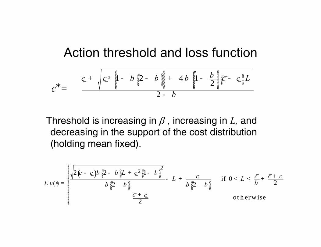
Action threshold and loss function

Threshold is increasing in β , increasing in L, and decreasing in the support of the cost distribution (holding mean fixed).

2

*1 2 4 1 2

2cc c c c Lbb b b

b

æ öé ù ÷çæ ö ÷ê ú ç æ ö÷÷ç ç ÷÷÷ê ú çç ç ÷÷÷ çç ç ÷ê ú ÷÷ çç ç ÷ç÷÷ è ø÷çê ú ç ÷è ø ÷ç ÷çê ú è øë û=+ - - + - -

-

( )2

22 2 1 if 0 2( ) 2 2

ot h er w ise2

c c L c c c c cL LE v

c c

b b bbb b b b

ìïïï æ ö æ öï ÷ ÷ç çï ÷ ÷ç çï ÷ ÷ç ç÷ ÷ï è ø è øïïï æ ö æ öï ÷ ÷ç çí ÷ ÷ç çï ÷ ÷ç ç÷ ÷ï è ø è øïïïïïïïïïî

- - + - +- + < < +× = - -

+

*c =

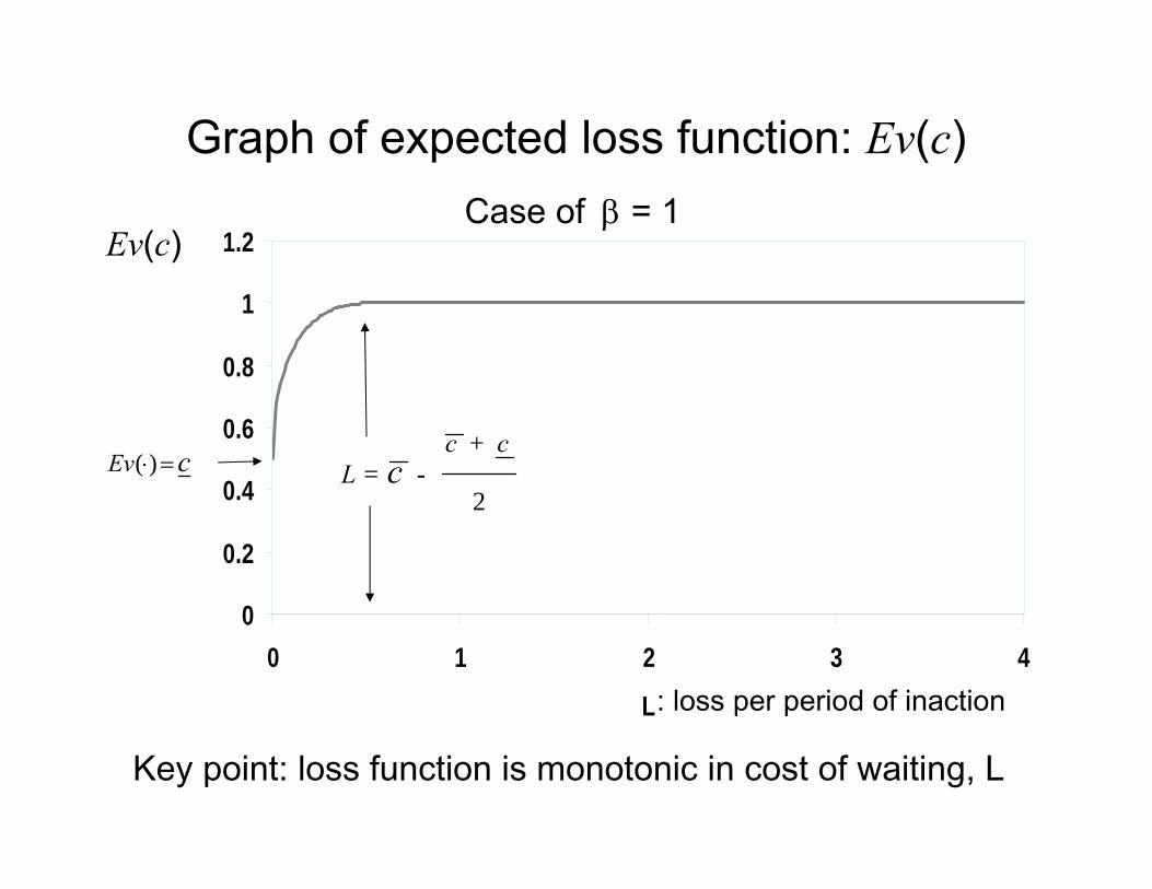
Graph of expected loss function: Ev(c)

0

0.2

0.4

0.6

0.8

1

1.2

0 1 2 3 4

L

Case of β = 1

0.5, 1.5c c= =

2

c cL c

+= -

Ev(c)

( )Ev c⋅ =

: loss per period of inaction

Key point: loss function is monotonic in cost of waiting, L

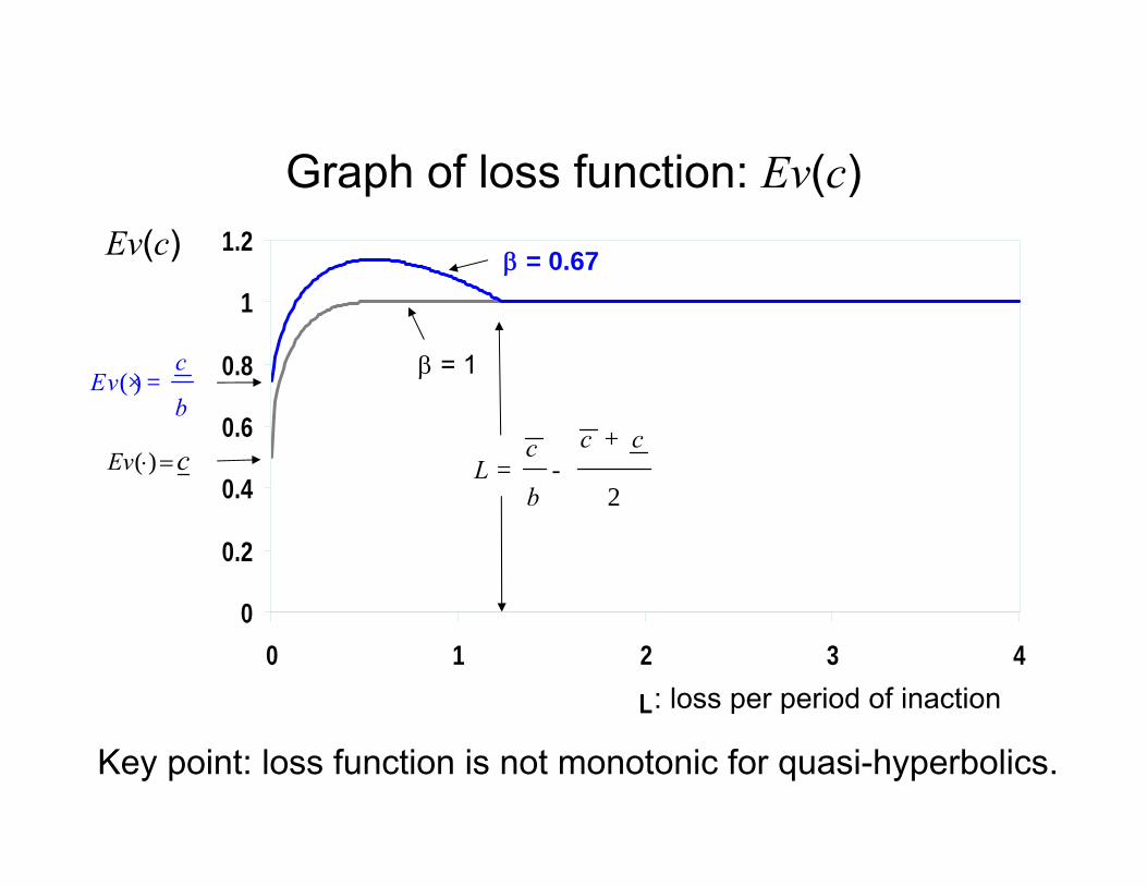
Graph of loss function: Ev(c)

0

0.2

0.4

0.6

0.8

1

1.2

0 1 2 3 4

L

β = 1

β = 0.67

0.5, 1.5c c= =

2

c ccL

b

+= -

( )c

Evb

× =

Ev(c)

( )Ev c⋅ =

: loss per period of inaction

Key point: loss function is not monotonic for quasi-hyperbolics.

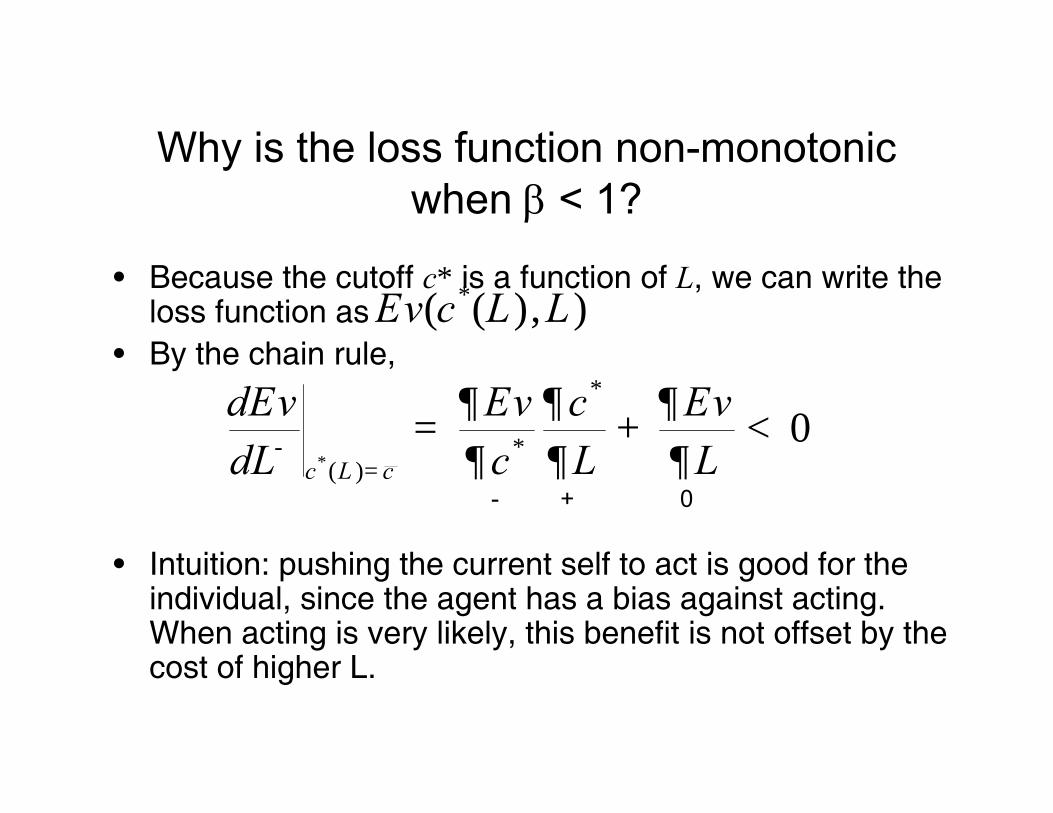
Why is the loss function non-monotonic when β < 1?

• Because the cutoff c* is a function of L, we can write the loss function as

• By the chain rule,

• Intuition: pushing the current self to act is good for the individual, since the agent has a bias against acting. When acting is very likely, this benefit is not offset by the cost of higher L.

*( ( ), )Ev c L L

*

*

*( )

0c L c

dEv Ev c EvdL c L L-

=

¶ ¶ ¶= + <¶ ¶ ¶

- + 0

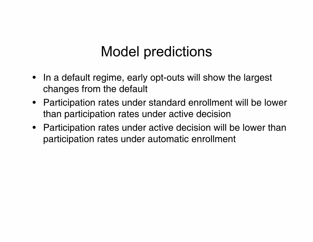
Model predictions

• In a default regime, early opt-outs will show the largest changes from the default

• Participation rates under standard enrollment will be lower than participation rates under active decision

• Participation rates under active decision will be lower than participation rates under automatic enrollment

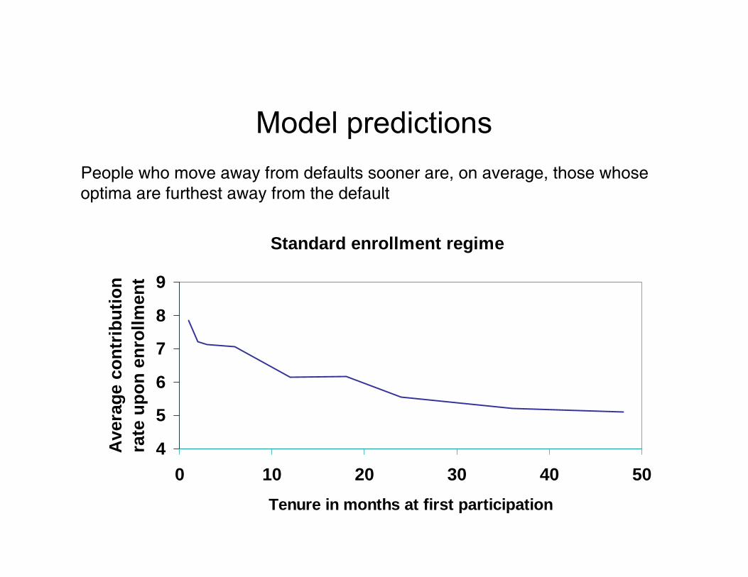
Model predictions

Standard enrollment regime

4

5

6

7

8

9

0 10 20 30 40 50Tenure in months at first participation

Ave

rage

con

trib

utio

n ra

te u

pon

enro

llmen

t

People who move away from defaults sooner are, on average, those whose optima are furthest away from the default

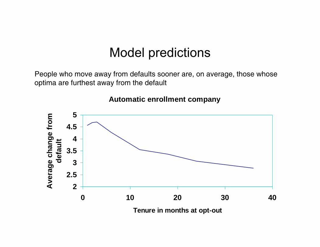
Model predictionsPeople who move away from defaults sooner are, on average, those whose optima are furthest away from the default

Automatic enrollment company

22.5

33.5

44.5

5

0 10 20 30 40Tenure in months at opt-out

Ave

rage

cha

nge

from

de

faul

t

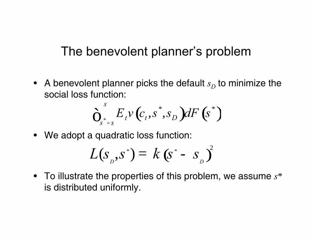
The benevolent planner’s problem

• A benevolent planner picks the default sD to minimize the social loss function:

• We adopt a quadratic loss function:

• To illustrate the properties of this problem, we assume s*is distributed uniformly.

( ) ( )*

* *, ,s

t t Ds sE v c s s dF s

=ò

( )* * 2( , )D D

L s s s sk= -

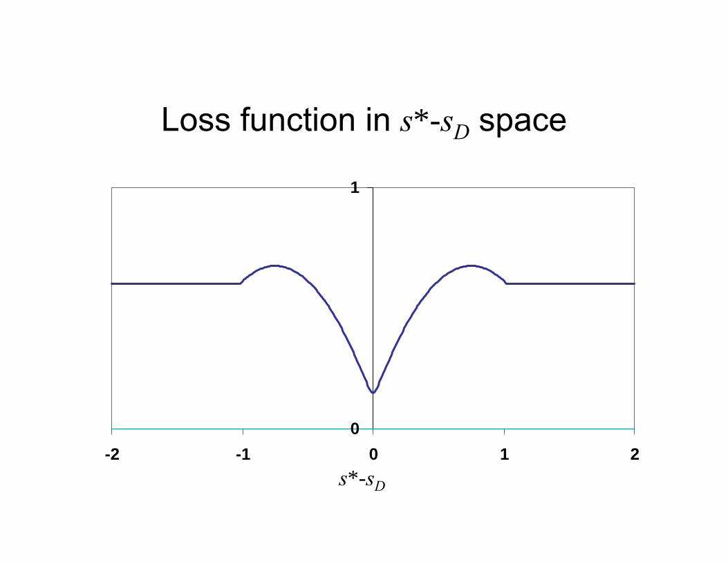
Loss function in s*-sD space

0

1

-2 -1 0 1 2s*-sD

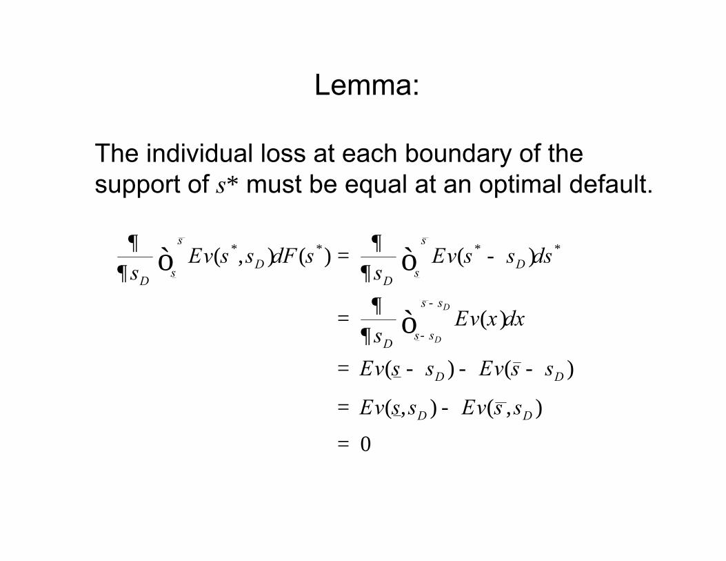
Lemma:

The individual loss at each boundary of the support of s* must be equal at an optimal default.

* * * *( , ) ( ) ( )

( )

( ) ( )

( , ) ( , )

0

D

D

s s

D Ds s

D D

s s

s sD

D D

D D

Ev s s dF s Ev s s dss s

Ev x dxsEv s s Ev s s

Ev s s Ev s s

-

-

¶ ¶= -¶ ¶

¶=¶

= - - -

= -

=

ò ò

ò

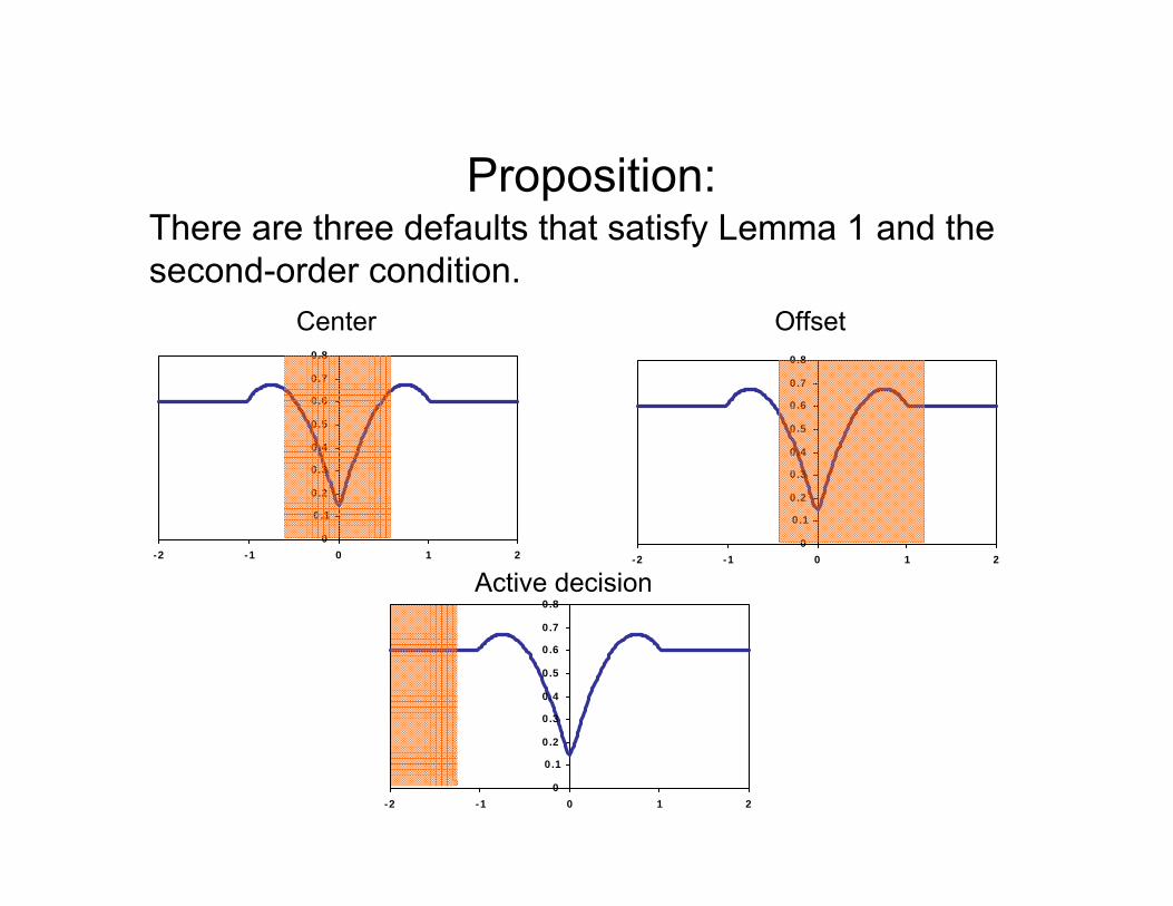
Proposition:There are three defaults that satisfy Lemma 1 and thesecond-order condition.

Center Offset

Active decision

0

0.1

0.2

0.3

0.4

0.5

0.6

0.7

0.8

-2 -1 0 1 20

0.1

0.2

0.3

0.4

0.5

0.6

0.7

0.8

-2 -1 0 1 2

0

0.1

0.2

0.3

0.4

0.5

0.6

0.7

0.8

-2 -1 0 1 2

Proposition:

Active decisions are optimal when:• Present-bias is large --- small β.• Average transaction cost is large.• Support of transaction cost is small.• Support of savings distribution is large.• Flow cost of deviating from optimal savings rate is

large (for small β).

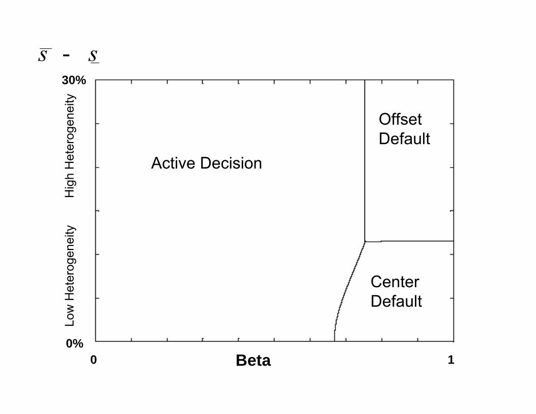
10 Beta

Active Decision

CenterDefault

OffsetDefault

30%

0%

Low

Het

erog

enei

ty

H

igh

Het

erog

enei

tys s-

Naives:

Proposition: For a given calibration, if the optimal mechanism for sophisticated agents is an active decision rule, then the optimal mechanism for naïve agents is also an active decision rule.

Example: Summary• Model of standard defaults and active decisions

– The cost of opting out is time-varying– Agents may be present-biased

• Active decision is socially optimal when…

− β is small– Support of savings distribution is large

• Otherwise, defaults are optimal

Talk summaryAlternative to revealed preferences• We should no longer rely on the classical theory of

revealed preferences to answer the fundamental question of what is in society's interest.

• Arbitrary contextual factors drive revealed preferences.

• Revealed preferences are not (always) normative preferences.

• We can do welfare economics without classical revealed preferences

Conclusions

• It’s easy to dramatically change savings behavior– Defaults, Active Decisions

• How should we design socially optimal institutions?1.Write down a positive model of behavior2.Estimate the model’s parameters3.Confirm that the model’s empirical accuracy4.Make assumptions about the relationship between

the positive model and normative preferences5.Design institutions that maximize normative

preferences, assuming that agents respond to the institutions according to the positive model