the regional spillover effects of the tohoku earthquake

C E N T E R O N J A P A N E S E E C O N O M Y A N D B U S I N E S S

Working Paper Series June 2016, No. 350

The Regional Spillover Effects of the Tohoku Earthquake

Robert Dekle, Eunpyo Hong, and Wei Xie

This paper is available online at www.gsb.columbia.edu/cjeb/research

C O L U M B I A U N I V E R S I T Y I N T H E C I T Y O F N E W Y O R K

The Regional Spillover Effects of the Tohoku

Earthquake∗

Robert Dekle†, Eunpyo Hong‡, and Wei Xie§

Department of Economics, Kaprielian Hall, USC

February 17, 2016

Abstract

In this paper, we trace out how a decline in industrial production inone region can be propagated throughout a country. We use the modelto measure how a shock to industrial production in Tohoku – owing tothe Earthquake and Tsunami from 2011 – can be propagated throughoutJapan. In our econometric model, regions and industries within regionsare linked by specific structures and these structures discipline how theshocks are spatially propagated.

Keyword:Tohoku earthquake, regional spillovers, industrial production, domi-nant region, propagation of shocksJEL Classification: R11 R15

∗We thank comments from Professors Etsuro Shioji and Walker Hanlon and participantsfrom the 2013 and 2014 Workshops at Gakushuiin Universities and USC. We thank the Centerfor Global Partnership for financial assistance.

†[email protected]‡[email protected]§[email protected]

1

1 Introduction

There is a large and growing literature relating aggregate fluctuations to id-iosyncratic disturbances (Dupor (1999); Acemoglu et al. (2012)). Economicunits – firms, regions, industries, etc. – are interrelated through input-outputrelationships or other spillovers such as technology. An idiosyncratic shock toone of the units can result in a large change in aggregate production if there arecomplementarities among the units such as input-output and other relationship-s. Whether the idiosyncratic shock can generate substantial aggregate volatilitydepends on the size of the initial shock, as well as the nature and strength ofthe linkages or the complementarities among the units.

While these linkages are potentially important, identifying plausible exoge-nous shocks to the individual units remains a challenge. This paper addressthis challenge by combining monthly industrial production data by industryand region with region-level exposure to a localized natural disaster, the GreatTohoku Earthquake of March 2011. We exploit the heterogeneous exposure ofregions to the earthquake and subsequent tsunami and their interrelationshipsto examine how the shock to Tohoku has been transmitted throughout Japan.We find that the maximal impact of earthquake on other Japanese regions hasoccurred in about 6 months. From aggregating the separate regional responses,we find that the Tohoku earthquake has lowered Japan’s nationwide industrialproduction by 6 percent in one month, 12 percent in 6 months, and 9.6 percentin 20 months.

On March 11, 2011, a devastating earthquake and tsunami hit the Tohokuand Northern Kanto regions of Japan. The damage was mostly concentrated inthe Iwate, Miyagi, and Fukushima prefectures. In particular, all three prefec-tures were swept by the tsunami, with much of the immediate damage causedby the tsunami. In the areas impacted by the tsunami, industrial productiondeclined by over 95 percent between March and July of 2011.

Nearly 23000 people were killed (or missing) in these prefectures; and inthe days after the earthquake, about 125,000 people (or 2 percent of the threeprefectures’ populations) evacuated. Destruction to the capital stock was esti-mated to be about $180 billion, or 10 percent of the total capital stock in thethree prefectures.

The overall weight of Iwate, Miyagi, and Fukushima in Japan is small, com-prising about 4 percent of both the Japanese population and GDP in 2010.Still the immediate impact of the earthquake and tsunami on Japanese aggre-gate production was huge, with the negative effect on aggregate GDP lingeringon for a year or more. This is because these three prefectures were major pro-ducers of electronics and other intermediate parts used for production in otherJapanese regions (and even the world), and the stoppage in production of theseintermediate parts meant that production of the final goods in the electronics,automotive, and other industries were stalled all over Japan. For example, To-hoku accounted for 42 percent of the micro-semiconductors and 40 percent ofthe flat screen filters used in the Japanese production of automobiles and cellphones.

2

The importance of this collapse in Tohoku intermediate input production canbe seen in how Japan’s aggregate GDP declined in the immediate aftermath ofthe earthquake. Compared to the previous quarter (before the earthquake),Japanese aggregate GDP declined by 1.9 percent in the first quarter of 2011.1

The declines in aggregate consumption and inventories contributed 0.9 and 0.6percent to the overall GDP decline, respectively.2 Inventories dropped sharply,as firms nationwide dug into their inventories to supply the intermediate parts– disrupted by the earthquake – necessary for production.

In subsequent quarters, while consumption recovered, inventories continuedtheir depletion. Between the last quarter of 2010 and the third quarter of2012, aggregate GDP grew by 0.5 percent. Aggregate consumption contributed1.2 percent to this growth, but the depletion of inventories and the decline innet exports contributed to dragging down GDP by 0.6 percent and 1.8 percentbetween the last quarter of 2010 and the third quarter of 2012.3 Exports declinedas production slowed and imports rose because of the need for raw materialsand construction materials for the reconstruction.

In this paper, we trace out how a decline in industrial production in oneregion can be propagated throughout Japan. We consistently estimate separateconditional error correction models for different regions of Japan, which we thensolve for a full set of spatio-temporal impulse response functions. Conditionalimpulse response analysis traces out the effects of shocks over time. However,with a spatial dimension, dependence is both spatial and temporal. In ourimpulse responses using our econometrically estimated model, we trace out theeffects from a shock to Tohoku.

In our econometric model, regions and industries within regions are linkedby a well defined structure and this structure disciplines how the shocks arespatially propagated. Our emphasis in part on the input-output structure inthe propagation of shocks after the Tohoku earthquake is motivated by thefact that much of the immediate impact of the Tohoku earthquake on otherregions was driven by the decline in intermediate inputs produced in Tohoku.

1It is important, however, to keep the magnitude of the impact of the Tohoku earthquakein perspective. In fact, the negative impact of the global financial crisis in late 2008 onoverall Japanese GDP was far larger than the negative impact of the Tohoku earthquake.Moreover, how the 2008 global financial crisis caused the Japanese recession at that time isvastly different from how the Tohoku earthquake caused the latest Japanese recession.

While the recession after the 2008 financial crisis was caused by a decline in Japanese invest-ment and an exogenous fall in exports, owing to a collapse in foreign demand, the recessionpost-earthquake was related to the inability of Japan to produce inputs to production, suchas intermediate products and energy, which led to a drawdown in inventories, a decline in theability to supply exports, and the increased imports of raw materials.

2 Let GDP=C+I. Then in an accounting sense, the contribution of variable C to the growthin GDP is approximately (C/GDP ) ∗∆C/C.

3During this longer period, net exports declined because of the fall in total exports andthe increase in total imports. The decline in total exports contributed to dragging down GDPgrowth by 0.6 percent and the rise in total imports contributed to dragging down GDP growthby 1.2 percent. Much of the increase in imports was driven by the increase in natural gasand other fossil fuel imports. Energy imports increased, since Japan was faced with an energyshortage. The energy shortage was caused by a shutdown of almost all of the country’s nuclearpower plants, which normally provides 30 percent of Japan’s total energy.

3

However, we also examine other structures linking regions such as technologicalspillovers. The shocks to Tohoku are propagated spatially to other regions. Theother regions in turn impact other regions with a delay. We also allow theselagged effects to echo back to Tohoku.

The literature examining the importance of the propagation of regionalshocks has followed two main approaches. The first strand is rooted in morestructural calibrated multi-regional models such as Caliendo et al. (2014) thatexplicitly take into account inter-regional linkages across sectors. This paperis in the second strand of the literature (Forni et al. (2000)) that relies ontime-series methods coupled with broad identifying restrictions among region-al linkages to assess the magnitude and propagation of regional shocks in theaggregate economy. The advantage of our approach is that it is flexible andallows for various types of regional linkages or economic distance measures a-mong regions. For example, one region may not be buying much from anotherregion, but may be strongly affected by a decline in industrial production inanother region if their technologies are similar. As another example, the outputof a region neighboring Tohoku may fall, not because the supply of industrialproducts from Tohoku fell, but because the demand from Tohoku declined. Ourflexible approach allows us the handle these varying forms of regional linkages.

This is not the first paper to trace out the effects of the earthquakes andother natural disasters on Japanese output and industrial production. Tokuiand Miyagawa (2014) examine how the distribution of economic activity withinJapan are impacted by natural disasters. Hosono et al. (2013) examine howshocks arising from earthquakes, when interacted with financing constraints,can lower firm-level industrial production.

Perhaps the paper most related to this work is Carvalho et al. (2014). Theauthors use firm-level data to try to quantify the impact of supply shocks e-manating from the Tohoku earthquake. They focus on existing firms in theearthquake affected areas and find that sales growth of linked firms outside thearea exhibit negative and significant effects for both upstream and downstreamfirms. While their data is much more detailed than ours (our data are regional,and their data are firm-level), the frequency of our data (monthly) is higherthan their frequency (annual). As we will see below, much of the propagation ofthe shocks occur at a frequency much below the annual; in our impulse responsefunctions, the maximal negative of the earthquake shock occurs nationwide inabout six months.

2 The Impact of the 2011 Tohoku Earthquakeon Aggregate and Regional Industrial Produc-tion

GDP includes a sizable component of non-manufacturing production, includingthe production of services. To better isolate the impact of the disruption ofthe production of parts in Tohoku on Japanese manufacturing production, for

4

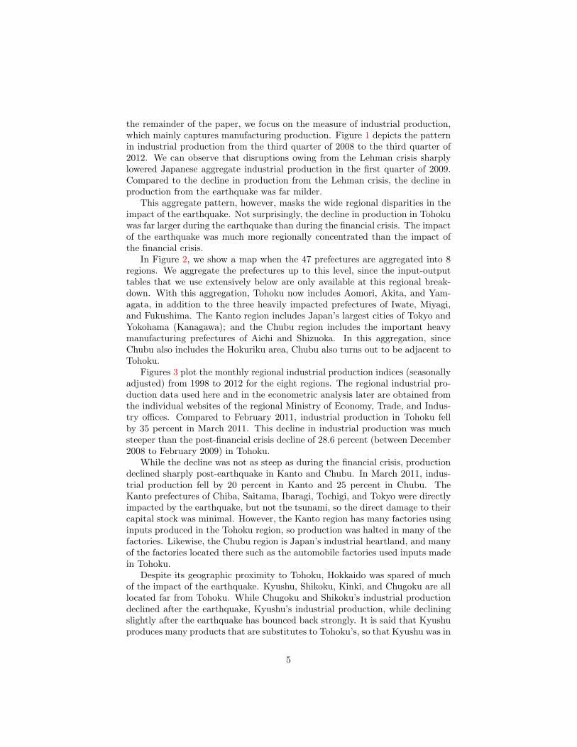
the remainder of the paper, we focus on the measure of industrial production,which mainly captures manufacturing production. Figure 1 depicts the patternin industrial production from the third quarter of 2008 to the third quarter of2012. We can observe that disruptions owing from the Lehman crisis sharplylowered Japanese aggregate industrial production in the first quarter of 2009.Compared to the decline in production from the Lehman crisis, the decline inproduction from the earthquake was far milder.

This aggregate pattern, however, masks the wide regional disparities in theimpact of the earthquake. Not surprisingly, the decline in production in Tohokuwas far larger during the earthquake than during the financial crisis. The impactof the earthquake was much more regionally concentrated than the impact ofthe financial crisis.

In Figure 2, we show a map when the 47 prefectures are aggregated into 8regions. We aggregate the prefectures up to this level, since the input-outputtables that we use extensively below are only available at this regional break-down. With this aggregation, Tohoku now includes Aomori, Akita, and Yam-agata, in addition to the three heavily impacted prefectures of Iwate, Miyagi,and Fukushima. The Kanto region includes Japan’s largest cities of Tokyo andYokohama (Kanagawa); and the Chubu region includes the important heavymanufacturing prefectures of Aichi and Shizuoka. In this aggregation, sinceChubu also includes the Hokuriku area, Chubu also turns out to be adjacent toTohoku.

Figures 3 plot the monthly regional industrial production indices (seasonallyadjusted) from 1998 to 2012 for the eight regions. The regional industrial pro-duction data used here and in the econometric analysis later are obtained fromthe individual websites of the regional Ministry of Economy, Trade, and Indus-try offices. Compared to February 2011, industrial production in Tohoku fellby 35 percent in March 2011. This decline in industrial production was muchsteeper than the post-financial crisis decline of 28.6 percent (between December2008 to February 2009) in Tohoku.

While the decline was not as steep as during the financial crisis, productiondeclined sharply post-earthquake in Kanto and Chubu. In March 2011, indus-trial production fell by 20 percent in Kanto and 25 percent in Chubu. TheKanto prefectures of Chiba, Saitama, Ibaragi, Tochigi, and Tokyo were directlyimpacted by the earthquake, but not the tsunami, so the direct damage to theircapital stock was minimal. However, the Kanto region has many factories usinginputs produced in the Tohoku region, so production was halted in many of thefactories. Likewise, the Chubu region is Japan’s industrial heartland, and manyof the factories located there such as the automobile factories used inputs madein Tohoku.

Despite its geographic proximity to Tohoku, Hokkaido was spared of muchof the impact of the earthquake. Kyushu, Shikoku, Kinki, and Chugoku are alllocated far from Tohoku. While Chugoku and Shikoku’s industrial productiondeclined after the earthquake, Kyushu’s industrial production, while decliningslightly after the earthquake has bounced back strongly. It is said that Kyushuproduces many products that are substitutes to Tohoku’s, so that Kyushu was in

5

fact a beneficiary of the damage to Tohoku’s production facilities. Surprisingly,Kinki, while including the industrial cities of Osaka and Kobe, was spared ofthe direct effects from the supply disruption of the intermediate parts producedin Tohoku.

3 Indices of Interactions Among Japanese Re-gions

As discussed above, the earthquake to Tohoku affected different regions in d-ifferent ways. Some regions like Kanto and Chubu experienced a sharp fall inindustrial production, while industrial production in Kinki, Chugoku, and otherSouthern regions barely budged. We have argued that the different propagationmechanisms in industrial production may be related to how different regionsused the inputs produced in Tohoku or were substitutes to the inputs producedin Tohoku.

In this Section, using input-output matrices that include 17 industries inour 8 regions, we show how the different regions in Japan are ”interrelated.”We consider five measures of ”interrelatedness.” The 17 industries and 8 regionsare depicted in Table 1. The measures of ”interrelatedness” are: 1) how tworegions are ”similar” (Conley and Dupor (2003)); 2) how much one region buysfrom another region (”buying” matrix); 3) how much one region sells to anotherregion; (”selling” matrix) 4) how much regions buy from each other (”mutualbuying” matrix); and 5) the geographical adjacency of two regions.

3.1 ”Interrelatedness” or Economic Distance Measures

We use the Japanese regional input-output matrices for 2005 compiled by RI-ETI, in which there are N = 8 regions. The raw input-output matrices includesrows (suppliers of commodities) and columns (purchasers of commodities) thatdo not correspond to any industries. On the column side, besides intermedi-ate users of commodities such as manufacturing, mining, and construction, theinput-output table contains columns for other components of gross domesticproduct: consumption, investment, change in business inventories, and govern-ment purchases. On the row side, the input-output table contains rows forcompensation to nonindustries such as wages and taxes. We address these com-ponents of the regional input-output table by: (a) removing all the final-usecolumns of the input-output table; and (b) dropping all additional rows of thetable. Finally, the original matrix has 29 industries, but we drop ”public ad-ministration”, ”medical services”, ”business services”, ”personal services”, and”others”, to arrive at M = 17 industries, which are primarily in manufacturing.

3.1.1 Notation

Γ is the input-output matrix of dimension N ×M by N ×M . A typical (s, b)-thelement of Γ is Γ(s, b), which is the total value of transactions between s’s supply

6

and b’s purchase. In other words, the s-th row of Γ corresponds to the value ofsales of s, and the b-th column of Γcorresponds to the value of purchases of b.

For i, j = 1, · · · , N and m,n = 1, · · · ,M , denote Γ(i(m), j(n)

)as the total

value of sales from region-i’s industry-m to region-j’s industry-n.

3.1.2 ”Similarity” Regional Matrix

This economic distance measure holds that two regions are close if they buygoods from similar industries (Conley and Dupor (2003)). We use the argumentthat regions with similar input requirements are likely to have similar technol-ogy; so that the same shock to a given region is likely to affect the output ofanother ”similar” region, through technological spillovers.

Steps to compute the ”similarity” matrix.

• calculate Bm

Bm(i, j) =Γ(i(m), j(m)

)∑k Γ

(k(m), j(m)

)• calculate B

B(i, j) =∑m

Bm(i, j)

• calculate Db

Db(i, j) =

{∑k

[B(k, i)−B(k, j)]2

}1/2

for i, j = 1, . . . .N .

This matrix is depicted in Table 2(a). According to this matrix, prefecturesmost related to Tohoku (in order) are: Kanto, Hokkaido, Kinki, Shikoku, Chubu,Chugoku, and Kyushu.

3.1.3 Buying Regional Matrix

Our second measure of ”interrelatedness” measures how much one region isbuying from another region.

X with (i, j)-the element

X (i, j) =

∑m,n Γ

(i(m), j(n)

)∑k,m,n Γ

(k(m), j(n)

)The term is the weight of sales from region i to region j among all the

regions’ sales to region j. This matrix is depicted in Table 2(b). If the firstregion is buying a lot from the second region, it means that the first regionhas a strong ”downstream” connection with the second region. According tothis matrix, prefectures most related to Tohoku (in order) are: Kanto, Chubu,Kinki, Chugoku, Kyushu, Hokkaido, Shikoku.

7

3.1.4 Selling Regional Matrix

Our third measure of ”interrelatedness” measures how much one region is sellingto another region.


X (i, j) =

∑m,n Γ

(i(m), j(n)

)∑l,m,n Γ

(i(m), l(n)

)The term is the weight of purchases by region j from region i among all

the regions’ purchases from region i. This matrix is depicted in Table 2(c).If the first region is selling a lot to the second region, it means that the firstregion has a strong ”upstream” connection with the second region. This typeof relationship among economic units is emphasized, for example, by Acemogluet al. (2012). According to this matrix, prefectures most related to Tohoku (inorder) are: Hokkaido, Kanto, Chubu, Kinki, Shikoku, Kyushu, Chugoku.

3.1.5 Mutual Buying Regional Matrix

In addition, our fourth measure of ”interrelatedness” measures how much tworegions are buying from each other, relative to their purchases from other region-s. The more the two regions are buying from each other, the more dependentor ”interrelated” are the two regions.


X (i, j) =

∑m,n Γ

(i(m), j(n)

)∑k,m,n Γ

(k(m), j(n)

) +

∑m,n Γ

(i(m), j(n)

)∑l,m,n Γ

(i(m), l(n)

)This matrix is depicted in Table 2(d). According to this matrix, prefectures

most related to Tohoku (in order) are: Kanto, Chubu, Kinki, Chugoku, Kyushu,Hokkaido, Shikoku.

3.1.6 Contiguity Matrix

The last matrix of ”interrelatedness” simply assigns a value of one if the regionshares a border with another region, deeming that if they share a border, theyare ”similar.” This matrix is depicted in Table 2(e). According to this matrix,prefectures most related to Tohoku (in order) are: Hokkaido, Kanto, Chubu,Kinki, Chugoku, Shikoku, and Kyushu.

4 Regional Spillover Effects

4.1 Model of Regional Spillover Effects

We employ the diffusion model of Holly et al. (2011) to assess the shock ofTohoku earthquake on the other regions in Japan. Holly et al. (2011) designed amethod for analyzing the spatial and temporal diffusion of shocks to a dominant

8

region, which was applied to evaluate the effects on UK housing prices due toshocks on the housing price to London. The method treats the house priceof London as a common factor and then models the contemporaneous as wellas lagged dependencies among regions conditional on London house prices.Weestimate using the monthly data of industrial production for the 8 Japan regionsdefined in the previous section. The data ranges from January 1998 to October2012, so that T = 178.

Denote pit as the industrial production data of region i at time t, for i =1, · · · , N and t = 1, · · · , T . The diffusion model has what is called the dominantregion (i = 1) and treats this region and the rest of the regions (i = 2, · · · , N)differently by allowing for the shock on the dominant region to affect the otherregions not only contemporaneously but also through lagged impacts, whileallowing for no contemporaneous effects from the rest of the regions on thedominant region.

For regions i = 2, · · · , N ,

∆pit = ϕis

(pi,t−1 − p̄si,t−1

)+ ϕi1 (pi,t−1 − p1,t−1) + ai

+

kia∑l=1

ail∆pi,t−l +

kib∑l=1

bil∆p̄si,t−l +

kic∑l=1

cil∆p1,t−l + ci0∆p1t + εit (1)

For region i = 1, ϕ11 and c10 are set to be 0 in the above equation (1), where

p̄sit =N∑j=1

Sijpjt, withN∑j=1

Sij = 1

That is, in region 1, the dominant region is not affected by the contempo-raneous shocks in any other region.In the estimation of the model above, wetake Kanto (Tokyo) as the dominant region. Tokyo’s industrial production isassumed to be only affected by its own lagged industrial production and thelagged effects of its neighbor’s industrial production. The industrial productionof other regions is assumed to be affected by not only the lagged effects of Tokyoand the remaining regions, but also the contemporary effects of the shocks toTokyo. The reason why we take Tokyo as the common factor is that on averageduring the period of the model’s estimation, 1998-2012, shocks to Tokyo wereclearly the most important for the whole of Japan, given that Tokyo’s GDP isabout 30 percent of Japan’s GDP4.

Sij ≥ 0 is the (i, j)-th element of weighted spatial matrix S, which measuresthe spatial connection between region i and region j. Note that the influenceof the other regions with exception of Kanto is entirely captured by p̄sit, which

4The ”common factor” approach to estimation treats the contemporaneous correlationsamong the regions by assuming that all the regions are affected by the common economy-wideshock, but with differing intensities. In our model, we treat the industrial production of thedominant region, Kanto, as the common factor. By doing so, we can consistently estimateerror correction models conditional on the common factor, Kanto’s industrial production,independently, region by region, and ignore the correlations among the error terms across theregions (Pesaran (2006)), εit.

9

weights the industrial productions of the other regions by the spatial weightingmatrix, Sij . Thus, p̄sit through the spatial weighting matrix captures how theshocks from say Tohoku, propagates to Kyushu. The structure of the spatialweighting matrix laid out in the previous section captures how two regions areinterrelated.

As pointed out by Holly et al. (2011), the error correcting specification ofequation (1) is a parsimonious representation of pair-wise cointegration of thedata across regions. In addition, weak exogeneity of ∆p1t in equation (1) canbe tested by the procedure of Wu (1973).

4.2 Spatio-temporal Impulse Response Functions

We can use the estimates from the model above to examine impulse responsesboth over time and space.The persistence profile of shocks to the system overtime and across regions can be evaluated using generalized impulse responsefunction (GIRF), initially advanced by Pesaran and Shin (1998).

For horizons h = 0, 1, · · · , the impulse response of a unit (i.e. a standarddeviation) shock on the dominant region is computed as

g1(h) = E(pt+h|ε1t =√σ11,Ft−1)− E(pt+h|Ft−1)

=√σ11ΨhRe1 (2)

where pt = (p1t, · · · , pNt)′ is the vector of industrial production data at

time t, Ft is the filtration of information up to time t, σ11 = var(ε1t), ande1 = (1, 0, · · · , 0)′. By stacking the N regressions in (1), Holly et al. (2011)derived that5

∆pt = a+Hpt−1 +

k∑l=1

(Al +Gl)∆pt−l +

k∑l=0

Cl∆pt−l + εt

where a, H, Al, Gl, and Cl are matrices of model parameters. It can be solvedfrom the above expression to get

∆pt = µ+Πpt−1 +

k∑l=1

γl∆pt−l +Rεt

where k = maxi{kia, kib, kic}, µ = Ra with R = (IN − C0)−1, Π = RH,

γl = R(Al +Gl +Cl).In a VAR form, this implies that

pt = µ+k+1∑l=1

Φlpt−l +Rεt

where Φ1 = IN +Π+ γ1, Φl = γl − γl−1 for l = 2, · · · , k and Φk+1 = −γk.

5See Holly et al. (2011) for detailed derivations of the generalized impulse response functionin the spatial temporal model.

10

Then for h = 0, 1, · · · , Ψh in equation (2) is defined as

Ψh =

k+1∑l=1

ΦlΨh−l

5 Empirical Results

5.1 Regions and their Connection

Kanto (Tokyo) is set as the dominant region in model (1) to account for bothof its contemporaneous and intertemporal impacts. Given the common fac-tor structure, we follow Holly et al. (2011) to estimate model (1) equation byequation using OLS.

Also, we construct the weighted spatial matrices based on our five measuresof regional ”interrelatedness” or economic distance.

5.2 Estimation Results

The estimation results are depicted in Table 3. Table 3(a) reports the resultsbased on the row standardized ”Similarity” matrix, Table 3(b) reports the re-sults based on the row standardized ”Buying” matrix, Table 3(c) reports theresults based on the row standardized ”Selling” matrix, Table 3(d) reports theresults based on the row standardized ”Mutual Buying” matrix, and Table 3(e)reports the results based on the row standardized ”Contiguity” matrix. We cansee that results from Table 3(a)-(e) are similar in the following ways.

”Own lag” is the estimated∑kia

l=1 ail. A positive ”own lag” effect implies thatthe series continues to drift in the same direction as the last period, exhibitingeither an upward trend or a downward trend. A negative ”own lag” effectimplies that the series adjusts to last period’s increase by a decrease in thecurrent period, exhibiting a property like mean reverting. Estimation basedon the ”Similarity” matrix identifies the own lag effects of Tohoku, Hokkaido,Chubu, Kinki, Chugoku, and Shikoku to be significant. Estimations based onthe ”Mutual Buying” matrix and the ”Contiguity” matrix identify the same setof significant own lag effects, ie. own lag effects are only found to be insignificantfor Kanto and Kyushu.

”Neighbour lag” estimates the dynamic spillover effects∑kib

l=1 bil. A positive”neighbour lag” effect implies that the series moves in the same direction as theweighted average of its neighbour in the last period. A negative ”neighbour lag”effect implies the series moves in the opposite direction. Both the estimationbased on the ”Similarity” matrix and the estimation based on the ”MutualBuying” matrix identify the same set of significant neighbour lag effects inHokkaido, Kinki, Chugoku, Shikoku, and Kyushu. Estimation based on the”Contiguity” matrix identifies significant neighbour lag effects in Chubu, Kinki,Chugoku, Shikoku, and Kyushu. Finally, based on all three ”interrelatedness”measures, the estimated neighbour lag effects on all the regions are positive,

11

except for the neighbour lag effect on Tohoku and the neighbour lag effect ofKanto when the Contiguity matrix is used as the ”interrelatedness” or economicdistance measure. Thus, for all five measures of ”interrelatedness” or economicdistance, industrial production shocks are positively correlated among regions,with the exception of Tohoku or Hokkaido.

With regards to the magnitudes of the ”neighbor” lags estimates, the ”sell-ing” matrix has the smallest coefficients, followed by the ”mutual buying ma-trix.” The ”selling” matrix captures how much the neighbors are buying fromthe region in question. The ”selling” matrix captures how much the industrialproduction of the upstream firm is affected by demand from the downstreamfirm.

”Kanto lag” is the estimated lagged effect of Kanto. A positive ”Kanto lag”effect implies that the series moved in the same direction as Kanto did in the lastperiod. Based on all the connectedness measures, the estimated ”Kanto lag”effects are found to be significantly positive for Tohoku. Significantly positive”Kanto lag” effects are also observed for Chubu when using the ”Similarity ma-trix” and ”Mutual buying matrix” and for Hokkaido when using the ”Contiguitymatrix”.

”Kanto current” is the estimated contemporaneous effect of Kanto, ci0. Apositive ”Kanto current” effect implies that the series simultaneously moves inthe same direction as Kanto. Based on all the connectedness measures, theestimated ”Kanto current” effects are similar, and all of them are significantlypositive.

EC1 is estimated ϕi1, which is referred to as the error correction term of(pi,t−1 − p1,t−1), the deviations of region i from Kanto. The estimated EC1are similar based on the three connectedness measures, which give a signifi-cantly negative EC1 for Chugoku; the Similarity matrix additionally identifiesthat Tohoku also has a significantly negative EC1. EC2 is the estimated ϕis,the error correction term of (pi,t−1 − p̄si,t−1), the deviation of region i from itsneighbours. The estimated EC2 based on the three ”interrelatedness measures”identify Chugoku and Shikoku to have significantly negative EC2; the ”MutualBuying matrix” and the ”Contiguity Matrix” both identify Tohoku to have asignificantly negative EC2.

WH-stat is the Wu-Hausman test statistics (Wu (1973)) testing the nullhypothesis that production changes in the dominant region Kanto are exogenousto production changes in the other regions. The results show that most of theregressions passed the Wu-Hausman test, except for the regression of Hokkaidobased on the ”Contiguity” matrix.

kia, kib, and kic are all selected by the Schwarz Bayesian criterion (SBC).Based on all three ”interrelatedness” measures, SBC selected kia to be equal to 1and kib to be equal to 1 or 2. SBC selected the lag orders kic = 0, producing theestimated ”Kanto lag” effects,

∑kic

l=1 cil, to be 0 for Kinki, Chugoku, Shikoku,and Kyushu.

12

5.3 Impulse Response Functions

Figures 4 to Figure 8 plot the estimated generalized impulse response functions(GIRF) caused by a 1 unit (i.e. 1 standard deviation) positive shock to Tohoku’sindustrial production.

The persistence profile of Tohoku shows that it takes about 2 years forTohoku to absorb 1/2 of a positive unit of shock to its monthly industrial pro-duction level. Interestingly, the impulse responses are quite similar across the”interrelatedness” measures. For example, across all five measures of econom-ic distance, the peak effect occurs in about 6 months, after which the effectsfrom the Tohoku industrial production shock declines. Across all five ”interre-latedness” measures, the largest impact of the Tohoku shock occurs in order, inChubu, Chugoku, Kyushu, Kinki, Kanto, and Shikoku. While the ordering ofthe impacts of the Tohoku shock do not differ by the ”interrelatedness” mea-sures, the magnitudes of the effects differ somewhat. For example, the largesteffect of the Tohoku shock on Chubu is highest when we use the economic dis-tance measure of ”buying” or ”mutual buying”. This suggests that Tohoku’srelationship with Chubu can be characterized as ”downstream”. That is, To-hoku buys a lot of intermediate inputs from Chubu.

This invariance of the regional propagation of shocks to the five econom-ic distance measures can also be seen in Figure 9. For selected time periodsh = 0, 3, 5, 10, 20, 50, Figure 9 depicts the Impulse Response functions across re-gions and over time. The regions are ordered on the horizontal axis from left toright according to their economic distance (according to each of the five ”inter-relatedness” matrices) to Tohoku. For example, in Figure 9(a), according to the”similarity” matrix, the ordered horizontal axis shows that the ”closest” regionto Tohoku is Kanto, followed by Hokkaido, Kinki, Shikoku, Chubu, Chugoku,and Kyushu.

If economic distance – according to our five definitions – results in higherspillovers, then we should see a declining pattern in the graphs. As the regionsbecome further from Tohoku, the impact of the Tohoku shock should dissipate.In general we see no such pattern in the graphs. As seen above, Chubu industrialproduction always has the largest response to a Tohoku industrial productionshock.

5.4 Quantification

Here we quantify the aggregate, nationwide effects of the Tohoku earth-quake and tsunami. During our sample period, a one standard deviation shockto Tohoku industrial production (IP) was about a 11 percent decline. As men-tioned, during the month of March 2011, Tohoku IP fell by 35 percent, whichis about a 3 standard deviation decline in Tohoku IP.

As seen above, the calculated impulse responses are generally invariant tothe five ”interrelatedness” or economic distance measures. Let us then withoutloss of generality, take the time series patterns and magnitudes from the impulseresponse functions from the ”mutual buying” matrix.

13

By taking the weighted sum of the eight region specific multipliers (from theimpulse responses), we can see that a one-standard deviation negative shock toTohoku IP will lower nationwide IP by 2.3 percent, 4 percent, and 3.2 percentin one, six, and twenty months. (The weights are from the region’s share ofaggregate IP. Kanto, for example, comprises about 39 percent of aggregate IP.)Multiplying these by 3 (the earthquake shock to Tohoku in standard deviations),the aggregate impact of the Tohoku earthquake are 6 percent, 12 percent, and9.6 percent in one, six, and twenty months.

6 Conclusion

In this paper, we traced out how a decline in industrial production in one regioncan be propagated throughout Japan. We examine how a shock to industrialproduction in Tohoku – owing to the earthquake – can be propagated throughoutJapan. In our econometric model, regions and industries within regions arelinked by specific measures of economic distance and these measures of economicdistance disciplines how the shocks are spatially propagated.

In general, while we definitely find effects on industrial production from theTohoku earthquake, the regional effects do not seem to depend much on our fivedefinitions of economic distance, although we observe significant heterogeneityin how different prefectures were affected by the spillovers from the Tohokuearthquake. For all economic distance measures, the effect of the Tohoku earth-quake and tsunami are largest on the Chubu region.

References

Acemoglu, D., Carvalho, V. M., Ozdaglar, A., and Tahbaz-Salehi, A. (2012).The network origins of aggregate fluctuations. Econometrica, 80(5).

Caliendo, L., Parro, F., Rossi-Hansberg, E., and Sarte, P.-D. (2014). The impactof regional and sectoral productivity changes on the u.s. economy. NBERWorking Paper 20168.

Carvalho, V. M., Nirei, M., and Saito, Y. (2014). Supply Chain Disruptions:Evidence from the Great East Japan Earthquake. Discussion papers 14035,Research Institute of Economy, Trade and Industry (RIETI).

Conley, T. G. and Dupor, B. (2003). A spatial analysis of sectoral complemen-tarity. Journal of Political Economy, 111(2):311–352.

Dupor, B. (1999). Aggregation and irrelevance in multi-sector models. Journalof Monetary Economics, 43(2):391 – 409.

Forni, M., Hallin, M., Lippi, M., and Reichlin, L. (2000). The generalizeddynamic-factor model: Identification and estimation. The Review of Eco-nomics and Statistics, 82(4):540–554.

14

Holly, S., Pesaran, M. H., and Yamagata, T. (2011). The spatial and temporaldiffusion of house prices in the uk. Journal of Urban Economics, 69(1):2 – 23.

Hosono, K., Miyakawa, D., Uchino, T., Hazama, M., Ono, A., Uchida, H., andUesugi, I. (2013). Natural disasters, damage to banks and firm investment.mimeographed.

Pesaran, H. H. and Shin, Y. (1998). Generalized impulse response analysis inlinear multivariate models. Economics Letters, 58(1):17–29.

Pesaran, M. H. (2006). Estimation and inference in large heterogeneous panelswith a multifactor error structure. Econometrica, 74(4):967–1012.

Tokui, J. K. K. and Miyagawa, T. (2014). Economic effects of the great japanearthquake. mimeographed, Gakushuiin University.

Wu, D.-M. (1973). Alternative tests of independence between stochastic regres-sors and disturbances. Econometrica, 41(4):733–50.

15

Table 1: Regions and Industries(a) Regions

01 Hokkaido02 Tohoku03 Kanto04 Chubu05 Kinki06 Chugoku07 Shikoku08 Kyushu + Okinawa

(b) Industries

020 Mining030 Beverages and Foods040 Textile products050 Timber, wooden products and furniture060 Pulp, paper, paperboard, building paper070 Chemical products080 Petroleum and coal products090 Plastic products100 Ceramic, stone and clay products110 Iron or steel products120 Non-ferrous metal products130 Metal products140 General machinery150 Electrical machinery160 Transportation equipment170 Precision instruments180 Miscellaneous manufacturing products

16

Table 2: Distance Measures(a) Similarity Matrix

Tohoku Hokkaido Kanto Chubu Kinki Chugoku Shikoku Kyushu

Kanto 0 11.366 12.227 13.034 12.703 14.064 12.999 13.905Tohoku 11.366 0 11.843 12.612 11.996 13.105 11.998 13.295Hokkaido 12.227 11.843 0 12.352 12.127 13.169 12.046 13.476Chubu 13.034 12.612 12.352 0 11.497 12.993 12.050 13.356Kinki 12.703 11.996 12.127 11.497 0 11.648 9.848 12.287

Chugoku 14.064 13.105 13.169 12.993 11.648 0 10.812 12.414Shikoku 12.999 11.998 12.046 12.050 9.848 10.812 0 11.796Kyushu 13.905 13.295 13.476 13.356 12.287 12.414 11.796 0

(b) Buying Matrix

Kanto Tohoku Hokkaido Chubu Kinki Chugoku Shikoku Kyushu



(c) Selling Matrix

Kanto Tohoku Hokkaido Chubu Kinki Chugoku Shikoku Kyushu



(d) Mutual Buying Matrix




(e) Contiguity Matrix


Tohoku 0 1 1 1 0 0 0 0Hokkaido 1 0 0 0 0 0 0 0Kanto 1 0 0 1 0 0 0 0Chubu 1 0 1 0 1 0 0 0Kinki 0 0 0 1 0 1 1 0

Chugoku 0 0 0 0 1 0 1 1Shikoku 0 0 0 0 1 1 0 1Kyushu 0 0 0 0 0 1 1 017

Table

3:Estim

ationresultsof

region

specificdiffusion

equationforTotal

Industrial

Production

(a)Sim

ilarity

Matrix

OwnLag

NeighbL

Kanto

Lag

Kanto

Curren

tEC1

EC2

Wu-H

aus

kia

kib

kic

Kanto

-0.3

(-2.624)

0.88(6.149)

--

--

-1

2-

Tohoku

-0.262(-3.253)

-0.026(-0.168)

0.442(3.220)

0.815(11)

--0.22(-3.653)

-0.815

11

1Hokkaid

-0.478(-6.518)

0.394(4.042)

-0.305(3.666)

--

1.134

11

0Chubu

-0.217(-3.031)

0.471(3.818)

-1.012(14.497)

--

0.263

11

0Kinki

-0.541(-4.785)

0.506(5.437)

-0.513(7.752)

--0.108(-2.343)

0.093

21

0Chugoku

-0.119(-1.394)

0.307(2.86)

-0.629(7.424)

--0.37(-4.561)

-0.632

11

0Shikoku

-0.59(-4.779)

0.519(3.319)

-0.526(4.192)

--

2.099

21

0Kyusyu

-0.059(-0.658)

0.1

(0.622)

0.366(2.896)

0.785(10.889)

--0.07(-2.138)

1.039

11

1(b

)BuyingMatrix

OwnLag

NeighbL

Kanto

Lag

Kanto

Curren

tEC1

EC2

Wu-H

aus

kia

kib

kic

Kanto

-0.293(-2.50)

0.867(6.02)

--

--

-1

2-

Tohoku

-0.252(-3.09)

-0.017(-0.09)

0.430(2.77)

0.817(11.19)

--0.237(-3.74)

-0.559

11

1Hokkaid

-0.478(-6.48)

0.370(3.93)

-0.323(3.93)

--

0.785

11

0Chubu

-0.230(-3.12)

0.489(3.86)

-1.004(14.26)

--

0.286

11

0Kinki

-0.567(-5.00)

0.218(1.82)

0.282(2.50)

0.560(8.36)

--0.113(-2.49)

-1.798

21

1Chugoku

-0.166(-1.98)

0.291(2.80)

-0.621(7.05)

--0.226(-3.45)

-1.008

11

0Shikoku

-0.593(-4.79)

0.019(0.07)

0.496(1.57)

0.594(4.49)

--

0.957

21

1Kyusyu

-0.270(-2.77)

0.250(1.95)

0.360(2.21)

0.826(11.44)

--

-0.675

21

1(c)SellingMatrix

OwnLag

NeighbL

Kanto

Lag

Kanto

Curren

tEC1

EC2

Wu-H

aus

kia

kib

kic

Kanto

-0.332(-2.61)

0.814(5.91)

--

--

-1

2-

Tohoku

-0.258(-3.09)

0.432(4.16)

-0.821(11.53)

--0.242(-3.46)

0.486

11

0Hokkaid

-0.481(-6.71)

0.401(4.58)

-0.330(4.13)

--

0.261

11

0Chubu

-0.282(-3.61)

0.557(4.31)

-1.013(14.83)

--

-0.265

11

0Kinki

-0.592(-5.02)

0.493(5.89)

-0.534(7.88)

--

-0.976

21

0Chugoku

-0.190(-2.21)

0.343(3.26)

-0.629(7.17)

--0.233(-3.32)

-0.904

11

0Shikoku

-0.617(-5.01)

0.562(3.75)

-0.523(4.25)

--

1.311

21

0Kyusyu

-0.257(-2.62)

0.601(5.37)

-0.783(11.07)

--

0.692

21

0(d

)Mutu

alBuyingMatrix

OwnLag

NeighbL

Kanto

Lag

Kanto

Curren

tEC1

EC2

Wu-H

aus

kia

kib

kic

Kanto

-0.309(-2.566)

0.868(6.022)

--

--

-1

2-

Tohoku

-0.254(-3.024)

0.445(4.132)

-0.810(11.391)

--0.254(-3.609)

0.387

11

0Hokkaid

-0.482(-6.703)

0.401(4.528)

-0.328(4.100)

--

0.527

11

0Chubu

-0.262(-3.432)

0.544(4.153)

-1.001(14.383)

--

0.142

11

0Kinki

-0.590(-5.111)

0.529(6.113)

-0.522(97.760)

--

-0.906

21

0Chugoku

-0.174(-2.048)

0.330(3.102)

-0.625(7.150)

--0.251(-3.569)

-0.912

11

0Shikoku

-0.617(-4.993)

0.563(3.698)

-0.519(4.187)

--

1.640

21

0Kyusyu

-0.252(-2.564)

0.607(5.283)

-0.780(10.996)

--

0.872

21

0(e)ContiguityMatrix

OwnLag

NeighbL

Kanto

Lag

Kanto

Curren

tEC1

EC2

Wu-H

aus

kia

kib

kic

Kanto

-0.159(-1.306)

0.576(4.82)

--

--

-1

2-

Tohoku

-0.216(-2.628)

-0.152(-1.038)

0.5

(3.444)

0.831(11.898)

--0.286(-4.098)

0.09

11

1Hokkaid

-0.454(-6.345)

-0.089(-1.064)

0.444(2.537)

0.373(4.696)

--

-0.699

11

1Chubu

-0.193(-2.603)

0.369(3.2)

-1.042(15.052)

--

-0.458

11

0Kinki

-0.570(-5.056)

0.114(1.245)

0.363(3.663)

0.574(8.578)

--0.104(-2.605)

-1.812

21

1Chugoku

-0.185(-2.303)

0.276(2.916)

-0.631(6.888)

-0.148(-2.882)

--1.649

11

0Shikoku

-0.292(-3.810)

-0.371(-1.554)

0.534(2.855)

0.677(4.925)

-0.097(-2.359)

--0.543

12

1Kyusyu

-0.252(-2.681)

0.146(2.142)

0.431(2.838)

0.831(11.597)

--

-1.027

21

1

Note:

Kan

to’s

lagg

edeff

ectare

estimated

tobe0an

dthusom

ittedfrom

thereport.

Lag

ordersareselected

separatelyby

SchwarzBayesiancriterionfrom

amax

imum

lagorder

of4.

18

Figure

1:Jap

aneseIndustrial

ProductionGrowth

(Quarterly,

sa)

−0

.25

−0

.2

−0

.15

−0

.1

−0

.050

0.0

5

0.1

2008Q3

2008Q4

2009Q1

2009Q2

2009Q3

2009Q4

2010Q1

2010Q2

2010Q3

2010Q4

2011Q1

2011Q2

2011Q3

2011Q4

2012Q1

2012Q2

2012Q3

Ind

ustr

ial P

rod

uctio

n G

row

th (

Qu

art

erly)

19

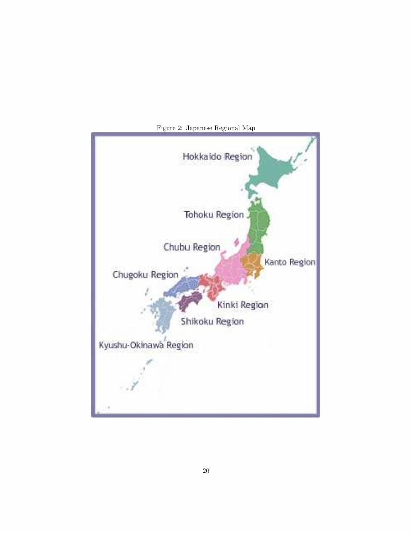
Figure 2: Japanese Regional Map

20

Figure

3:Tim

eSeriesPlotof

Total

Industrial

ProductionData

Tim

e

2000

2005

2010

7090110To

hoku

Hok

kaid

oK

anto

Chu

bu

Tim

e

2000

2005

2010

7090110

Kin

kiC

hugo

kuS

hiko

kuKy

ushu

21

Figure 4: Shock on IP based on Similarity matrix

0 10 20 30 400

0.5

1

Kanto90% Bootstrap Bound

0 10 20 30 400

1

2

Tohoku90% Bootstrap Bound

0 10 20 30 400

0.5

1

Hokkaido90% Bootstrap Bound

0 10 20 30 400

0.5

1

1.5

Chubu90% Bootstrap Bound

0 10 20 30 400

0.5

1

Kinki90% Bootstrap Bound

0 10 20 30 400

0.5

1

Chugoku90% Bootstrap Bound

0 10 20 30 40−0.5

0

0.5

1

Shikoku90% Bootstrap Bound

0 10 20 30 400

0.5

1

1.5

Kyushu90% Bootstrap Bound

22

Figure 5: Shock on IP based on Buying Matrix

0 10 20 30 400

0.5

1


0 10 20 30 400

1

2


0 10 20 30 400

0.5

1


0 10 20 30 400

0.5

1

1.5


0 10 20 30 400

0.5

1


0 10 20 30 400

0.5

1


0 10 20 30 40−0.5

0

0.5

1


0 10 20 30 400

0.5

1

1.5


23

Figure 6: Shock on IP based on Selling Matrix

0 10 20 30 400

0.5

1


0 10 20 30 400

1

2


0 10 20 30 400

0.5

1


0 10 20 30 400

0.5

1

1.5


0 10 20 30 400

0.5

1


0 10 20 30 400

0.5

1


0 10 20 30 40−0.5

0

0.5

1


0 10 20 30 400

0.5

1

1.5


24

Figure 7: Shock on IP based on Mutual Buying Matrix

0 10 20 30 400

0.5

1


0 10 20 30 400

1

2


0 10 20 30 400

0.5

1


0 10 20 30 400

0.5

1

1.5


0 10 20 30 400

0.5

1


0 10 20 30 400

0.5

1

1.5


0 10 20 30 40−0.5

0

0.5

1


0 10 20 30 400

0.5

1

1.5


25

Figure 8: Shock on IP based on Contiguity Matrix

0 10 20 30 400

0.5

1


0 10 20 30 400

1

2


0 10 20 30 40−0.5

0

0.5

1


0 10 20 30 400

0.5

1

1.5


0 10 20 30 400

0.5

1


0 10 20 30 400

0.5

1


0 10 20 30 40−1

−0.5

0

0.5


0 10 20 30 400

0.5

1

1.5


26

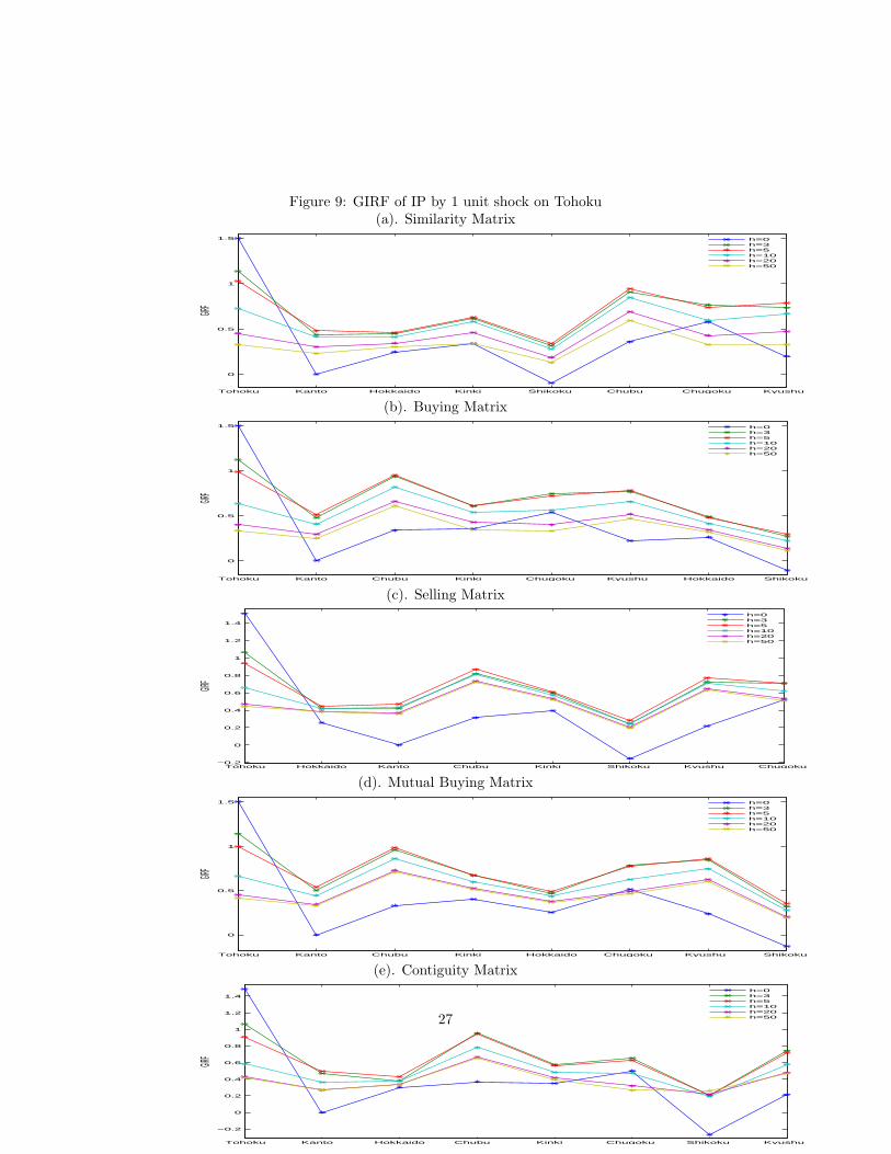
Figure 9: GIRF of IP by 1 unit shock on Tohoku(a). Similarity Matrix

Tohoku Kanto Hokkaido Kinki Shikoku Chubu Chugoku Kyushu

0

0.5

1

1.5

GIRF

h=0h=3h=5h=10h=20h=50

(b). Buying Matrix

Tohoku Kanto Chubu Kinki Chugoku Kyushu Hokkaido Shikoku

0

0.5

1

1.5

GIRF

h=0h=3h=5h=10h=20h=50

(c). Selling Matrix

Tohoku Hokkaido Kanto Chubu Kinki Shikoku Kyushu Chugoku −0.2

0

0.2

0.4

0.6

0.8

1

1.2

1.4

GIRF

h=0h=3h=5h=10h=20h=50

(d). Mutual Buying Matrix

Tohoku Kanto Chubu Kinki Hokkaido Chugoku Kyushu Shikoku

0

0.5

1

1.5

GIRF

h=0h=3h=5h=10h=20h=50

(e). Contiguity Matrix

Tohoku Kanto Hokkaido Chubu Kinki Chugoku Shikoku Kyushu

−0.2

0

0.2

0.4

0.6

0.8

1

1.2

1.4

GIRF

h=0h=3h=5h=10h=20h=5027

the regional spillover effects of the tohoku earthquake

Documents