the polish instrument - caltechthesisthesis.library.caltech.edu/857/3/02chapter2.pdfthe polish...

25

Chapter 2

The POLISH Instrument

2.1 Introduction

While most astrophysical objects require many parameters in order to be fully described, black holes

are unique in that only three parameters suffice: mass, spin, and charge. Mass and spin describe

the black hole’s gravitational field and event horizon location. Therefore, black holes provide a rare

opportunity for theory and observation to jointly pursue two quantities to completely describe one

of the most exotic kinds of objects in the Universe.

Though observational and modeling precision is somewhat effective in constraining black hole

spin (McClintock et al. 2006), important constraints on black hole mass exist in the case of high

mass X-ray binaries (hereafter HMXBs). These binaries consist of an O or B type supergiant and a

black hole or neutron star. The most well-studied of these, Cygnus X-1, is thought to consist of a

40± 10 M�, O9.7Iab star and a 13.5− 29 M� black hole at a distance of 2.2± 0.2 kpc (Ziolkowski

2005). While the constraints on the mass of the compact object are tight enough to declare that it

is a black hole, they are insufficient to permit precise modeling of the progenitor star’s mass. We

have commissioned a polarimeter on the Hale 5-m telescope at Palomar Observatory in California to

provide an independent method for determining black hole mass. This polarimeter has the potential

to constrain the mass of the Cygnus X-1 black hole to a few solar masses.

1The following paper is derived from this chapter: Wiktorowicz, S. J. & Matthews, K. 2008, PASP, 120, 1282.

26

2.2 Black Hole Mass from Polarimetry

A wealth of radial velocity data exists for Cygnus X-1 (Gies et al. 2003) and other HMXBs. However,

in the same way that precise masses are elusive for non-transiting extrasolar planets, determination

of precise black hole mass is hindered by unknown orbital inclination. This is evidenced by the end

product of radial velocity observations, the so-called “mass function”. For Cygnus X-1, Gies et al.

(2003) quote the following value:

f (MX) =Mopt sin3 i

q (1 + q)2 = 0.251± 0.007M�. (2.1)

Here, MX is the mass of the black hole, Mopt is the mass of the visible binary component, i is the

system inclination, and q is the mass ratio of the visible component to the black hole. Thus, an

observational technique to constrain orbital inclination can take advantage of radial velocity data

and offer an estimate of black hole mass.

Since system polarization is a geometric effect, the polarization of an HMXB system can be used

to determine geometric information about the system, such as orbital inclination. The effective

temperature of the supergiant in an HMXB is Teff ≈ 30,000 K, which is hot enough to ionize

photospheric hydrogen. This causes a high density of free electrons that Thomson-scatter emitted

light from the supergiant. While net linear polarization from a spherical cloud of free electrons is

zero, asymmetry in the system causes net polarization. The tidal effects of the black hole cause such

an asymmetry in the circumbinary envelope, and the orbital modulation of polarization is the key

to determining orbital inclination. For instance, consider a face-on HMXB with zero eccentricity

and an optically thin circumbinary envelope (Figure 2.1a). The total amount of observed polarized

light is independent of orbital phase, and the degree of polarization is therefore constant. However,

the angle of net polarization rotates as the binary progresses in its orbit.

In contrast, for a nearly edge-on geometry the degree of polarization varies significantly through-

out the orbit, while the angle of net polarization is roughly constant (Figure 2.1b). Therefore, the

modulation of the degree and angle of net polarization is a unique measure of orbital inclination for

synchronously rotating HMXBs. Combining Equations 1 and 2 from Friend & Cassinelli (1986) and

Equation 2 from Brown et al. (2000), the polarization of an axisymmetric envelope due to Thomson

scattering is

27

Figure 2.1: Orbital modulation of system polarization for HMXBs. The degree of polarization isrepresented by the black tidal bulges (the exact cause of polarization is irrelevant to this figure),and position angle of net polarization is given by the orientation of the grey lines. The face-on caseis shown in (a), and the edge-on case is shown in (b). The circumbinary envelopes have been drawndisplaced from the center of mass for clarity.

P =316σT(1− cos2 φorb sin2 i

) ∫ r2

r1

∫ µ2

µ1

ne (r)(

1− R2

r2

) 12 (

1− 3µ2)drdµ. (2.2)

Here, stellar radius is R, the electron number density is ne (r) = noR2/r2, system inclination is i,

and orbital phase in radians is φorb. Two polarization periods occur per orbital period, because of

the cos2 φorb term.

This technique has been utilized by a few groups (Kemp et al. 1979, Dolan & Tapia 1989, Wolinski

et al. 1996), and Cygnus X-1 has been found to have variable polarization of order ∆P ≈ 0.1% of

its unpolarized flux. However, measurement precision from the above groups is of order one part

in 104. The derived inclination estimates were questioned by the community (Milgrom 1979, Aspin

et al. 1981) on the grounds that significant underestimation of error occurred because of limited

measurement precision. Measuring inclination to 5◦ requires polarimetric precision of one part in

104 to one part in 107 (Aspin et al. 1981), depending on system inclination. This requires at least

108 to 1014 detected photons, which necessitates the use of 4-m class telescopes. Since our system

combines a high precision instrument with a 5-m telescope, we aim to measure the polarimetric

variability of Cygnus X-1 to better than one part in 104.

28

PEM(+45°)

PEM(-45°)

Beam-splitter

WollastonFieldlens

Detector2

Detector1

!TelescopeBeam

Figure 2.2: Plan view of the POLISH optical path. The telescope beam is directed into the pagethrough the center of the PEM aperture (the “X” in the figure). The PEM is rotated to θPEM = ±45◦

with respect to the centerline, and the instrument itself (dotted box) can be independently rotatedon the telescope through ∆φ = 360◦. Field stops are located between the field lenses and detectors.

2.3 The Polarimeter

Polarimeters require the following fundamental components: a polarization modulator, analyzer, de-

tector, and demodulator. The modulator induces a known, periodic characteristic to the unknown

polarization of the input beam. The analyzer converts modulation in polarization to modulation in

the beam’s intensity, since most detectors are sensitive to intensity and not polarization. Finally, the

demodulator extracts the component of the detector’s output that varies at the known frequency of

the modulator to reject noise. See Figure 2.2 for a block diagram, Figure 2.3 for a ray trace diagram,

and Figure 2.4 for photographs of the instrument.

Traditionally, the modulator is a rotating halfwave plate that rotates the linear polarization of

the incident beam. The highest modulation frequency attainable with this component is of order

100 Hz, which is not fast enough to freeze out atmospheric turbulence or to mitigate electronic 1/f

noise. Additionally, inhomogeneity in both the retardance and cleanliness of the plate can intro-

duce spurious signals, because the beam samples different sections of the halfwave plate at different

times. The polarization goal for our instrument, POLISH (POLarimeter for Inclination Studies of

29

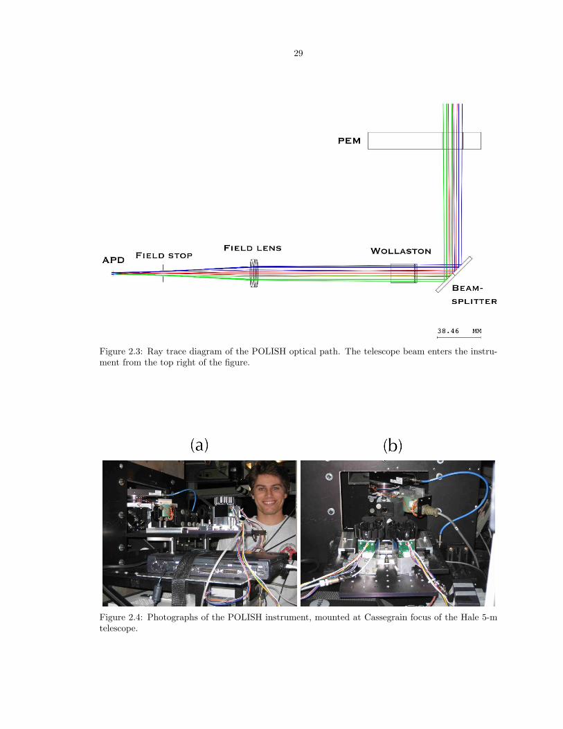
Figure 2.3: Ray trace diagram of the POLISH optical path. The telescope beam enters the instru-ment from the top right of the figure.

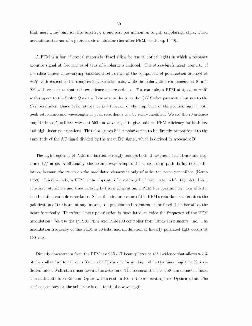
Figure 2.4: Photographs of the POLISH instrument, mounted at Cassegrain focus of the Hale 5-mtelescope.

30

High mass x-ray binaries/Hot jupiters), is one part per million on bright, unpolarized stars, which

necessitates the use of a photoelastic modulator (hereafter PEM; see Kemp 1969).

A PEM is a bar of optical materials (fused silica for use in optical light) in which a resonant

acoustic signal at frequencies of tens of kilohertz is induced. The stress-birefringent property of

the silica causes time-varying, sinusoidal retardance of the component of polarization oriented at

±45◦ with respect to the compression/extension axis, while the polarization components at 0◦ and

90◦ with respect to that axis experiences no retardance. For example, a PEM at θPEM = ±45◦

with respect to the Stokes Q axis will cause retardance to the Q/I Stokes parameter but not to the

U/I parameter. Since peak retardance is a function of the amplitude of the acoustic signal, both

peak retardance and wavelength of peak retardance can be easily modified. We set the retardance

amplitude to β0 = 0.383 waves at 500 nm wavelength to give uniform PEM efficiency for both low

and high linear polarizations. This also causes linear polarization to be directly proportional to the

amplitude of the AC signal divided by the mean DC signal, which is derived in Appendix B.

The high frequency of PEM modulation strongly reduces both atmospheric turbulence and elec-

tronic 1/f noise. Additionally, the beam always samples the same optical path during the modu-

lation, because the strain on the modulator element is only of order ten parts per million (Kemp

1969). Operationally, a PEM is the opposite of a rotating halfwave plate: while the plate has a

constant retardance and time-variable fast axis orientation, a PEM has constant fast axis orienta-

tion but time-variable retardance. Since the absolute value of the PEM’s retardance determines the

polarization of the beam at any instant, compression and extension of the fused silica bar affect the

beam identically. Therefore, linear polarization is modulated at twice the frequency of the PEM

modulation. We use the I/FS50 PEM and PEM100 controller from Hinds Instruments, Inc. The

modulation frequency of this PEM is 50 kHz, and modulation of linearly polarized light occurs at

100 kHz.

Directly downstream from the PEM is a 95R/5T beamsplitter at 45◦ incidence that allows ≈ 5%

of the stellar flux to fall on a Xybion CCD camera for guiding, while the remaining ≈ 95% is re-

flected into a Wollaston prism toward the detectors. The beamsplitter has a 50-mm diameter, fused

silica substrate from Edmund Optics with a custom 400 to 700 nm coating from Opticorp, Inc. The

surface accuracy on the substrate is one-tenth of a wavelength.

31

We utilize a two-wedge, calcite Wollaston prism from Karl Lambert, Inc., as our analyzer. This

prism separates each component of a single Stokes parameter into two beams. That is, the +Q/I (or

+U/I) component is split into one beam, and the −Q/I (or −U/I) component is in the other beam.

Both beams have equal deviation of 7.5◦ from the optical axis, which allows the optical layout to

be symmetric with respect to the optical axis. A two-wedge prism is used because the larger beam

deviation of a three-wedge design would cause the instrument package to be larger than necessary.

The surfaces of the Wollaston prism have an antireflection coating in the wavelength range 400 to

700 nm. The transmission in V band is ≈ 97% per surface. By injecting light through a linear

polarizer with known fast axis orientation and then through the Wollaston prism, we find that the

left beam seen from downstream is vertically polarized (−Q/I when projected onto the sky for a

Cassegrain ring angle of 0◦). The right beam is horizontally polarized (+Q/I at 0◦ ring angle).

Each Wollaston beam then impinges on an f/5.6, MgF2 antireflection-coated field lens from

Melles Griot. These lenses image the telescope secondary mirror onto the detectors, and they ensure

starlight is uniformly spread over the detector active area even in the presence of image wander.

Field stops are located in the image plane, after the field lenses, but these are not currently used

because contamination of stellar polarization from the sky field is not significant. The beams reach

the detectors with a diameter of ≈ 3 mm, which underfills all detectors.

Since Cygnus X-1 has V magnitude ≈ 9, but the polarization standard stars we observe can be

as bright as V ≈ 3, POLISH has two interchangeable pairs of detectors. Stars fainter than V ≈ 7

are detected at a higher signal to noise ratio with the pair of Hamamatsu H9307-04 photomulti-

plier tubes (PMTs), while objects brighter than this will destroy the PMTs. The brighter stars are

observed with custom-made Advanced Photonix SD197-70-72-661 (red enhanced) and SD197-70-74-

661 (blue enhanced) avalanche photodiode modules (APDs). The high quantum efficiency of APDs

is desirable on bright stars to minimize photon shot noise, while the low dark current of PMTs is

desirable on fainter stars to minimize detector noise.

Since these detectors are not downstream from spectral filters, they are integrated light detec-

tors in both spatial and spectral senses. Spatial resolution is unnecessary, as the angular size of the

Cygnus X-1 system is much smaller than the atmospheric seeing disk. Spectral resolution, while

desirable, would seriously degrade the precision attainable with this instrument. Such resolution

must be left for future generations of POLISH. The instrumental throughput is calculated to be

32

74%, 77%, 58%, and 23% in B, V , R, and I bands. The throughput of the telescope/instrument

system is calculated to be 60%, 62%, 47%, and 19% in those bands.

The PMTs are identical, side-on modules with active area dimensions 3.7 × 13.0 mm. Their

quantum efficiencies are quoted from the manufacturer to be 18%, 15%, 7%, and 0% in B, V , R,

and I bands. The PMT gain can be set by a potentiometer, and we set this gain to G = 5× 106 for

all observations. The modules also have a B = 200 kHz bandwidth amplifier with transimpedance

TA = 105 V/A. The quoted output noise voltage resulting from dark current is σ′V = 10 (typical) to

100 µV (maximum), which implies a noise equivalent power of NEP = 0.04 to 0.13 fW/√

Hz. Dark

current is i′d = 0.1 nA.

The APDs are custom-built from Advanced Photonix, Inc., and have 5 mm diameter, circular

active areas. Customization of the APDs allowed lower noise at the frequency of linear polarization

modulation. The APDs are not identical, as one beam is sampled by the red enhanced module while

the other is sampled by the blue enhanced one. The quantum efficiencies for the red enhanced mod-

ule are quoted as 24%, 62%, 88%, and 75% in B, V , R, and I bands. The blue enhanced module is

quoted to have 75%, 82%, 67%, and 35% quantum efficiencies. The blue module operates at a quoted

gain of G = 300, and the red module operates with an observed gain of G = 220. Transimpedance is

TA = 4× 106 V/A for both modules, and amplifier bandwidth is B = 100 kHz for the red enhanced

and B = 90 kHz for the blue enhanced modules. After the APD chip is thermoelectrically cooled

to 0◦ C, dark current is measured to be i′d = 4.5 nA and 3.5 nA at the output of the red and blue

modules, respectively. Therefore, the noise equivalent power for each module is NEP = 39 fW/√

Hz

and 9.7 fW/√

Hz, respectively. Each detector is supplied ±12V and +5V, and a 12V case fan blows

heat from the APD heat sinks to keep current draw stable.

The demodulator picks out the component of the detected signal that varies at the reference

frequency and ideally rejects signals at all other frequencies. The demodulator can either be software

or hardware; POLISH makes use of one Stanford Research SR830 digital, dual-phase lock-in amplifier

for each detector. The PEM controller sends a square wave reference signal to the lock-in amplifiers

at twice the frequency of the PEM modulation, and each lock-in amplifier recovers X (in phase with

reference signal) and Y (90◦ out of phase with the reference signal) components of the detector signal.

Together, X and Y determine amplitude R and phase Φ of the detector signal whose modulation

frequency is the same as the reference.

33

Table 2.1: Stokes Parameters Given by Positive AC Phase

Cassegrain angle (◦) Left Beam (Detector 2) Right Beam (Detector 1)0 −Q/I +Q/I45 −U/I +U/I90 +Q/I −Q/I135 +U/I −U/I180 −Q/I +Q/I225 −U/I +U/I270 +Q/I −Q/I315 +U/I −U/I

R =√

2 (X2 + Y 2) (2.3a)

Φ =12

arctan (Y,X) (2.3b)

The lock-in amplifiers record the RMS components of the in-phase and quadrature phase signals,

so multiplication by a factor of√

2 is necessary to determine the amplitude of the AC signal. The

notation of the argument of the arctangent is meant to account for signs of X and Y when deter-

mining phase.

Signal phase allows direct measurement of the sign of each Stokes parameter (+Q/I versus −Q/I,

for instance). This is important, because insensitivity to sign would preclude direct measurement of

more than 90◦ of rotation of the Cygnus X-1 system. By placing a linear polarizer with known axis

orientation in front of the PEM, we have determined the Stokes parameter sampled by each beam

as a function of Cassegrain ring angle. See Table 2.1 for a list of parameters measured for positive

AC phase.

Both AC and DC signals from the detector must be recorded to measure polarization (Appendix

B). The AC signals are recorded by the lock-in amplifiers, and each detector’s DC signal is recorded

by a separate HP 34401A digital voltmeter. The time constant and sampling frequency of the lock-in

amplifiers, as well as the sampling frequency of the voltmeters, must be chosen with care. To reject

60 Hz noise and its harmonics, each DC reading by the voltmeters consists of an integration over

10 power line cycles. Thus, the voltmeters record data at 6 Hz. The lock-in amplifiers may only

34

sample the AC signal at powers of two in frequency, so we choose to record the AC data at 8 Hz.

The discrepancy in sampling rates between AC and DC data is not important, because AC data

should be normalized by mean DC data and not in a point-by-point fashion.

In order to Nyquist sample the AC data, we set the lock-in time constants to 30 ms. For the

steepest filter rolloff, 24 dB/octave, the effective noise bandwidth is given by ENBW = 5/(64τ),

where τ is the lock-in amplifier’s time constant. For a time constant of 30 ms, ENBW = 2.6 Hz.

Therefore, we sample the AC data 8/2.6 ≈ 3.1 times per effective time constant, which both satisfies

the Nyquist criterion and reduces aliasing. The lock-in amplifiers therefore measure the component

of the AC signal that varies in the frequency range f0

(1± 1.3× 10−5

), where f0 is the reference

frequency. The auxiliary DC output of one lock-in amplifier is connected to a chopping motor on

the telescope secondary mirror. This lock-in amplifier sends a voltage signal to the secondary mirror

chopping motor, which causes the secondary mirror to chop north to a sky field for sky subtraction

of both AC and DC data.

POLISH is located at Cassegrain focus to ensure beam reflections of ≈ 180◦. In addition, the in-

strument resides at the f/72 focus. Both of these steps minimize telescope polarization. To minimize

instrument polarization, the first optic the beam encounters after the telescope secondary mirror is

the PEM. The lock-in amplifiers and voltmeters are controlled by a laptop, which is mounted to the

instrument, via the GPIB interface. Matlab R2006a from The MathWorks, Inc., is used to control

the voltmeters and lock-in amplifiers, chop the secondary mirror, and rotate the Cassegrain ring to

allow access to both linear Stokes parameters.

2.4 Observing Strategy

A similar, albeit larger, instrument called PlanetPol is mounted on the 4.2-m William Herschel Tele-

scope in La Palma, Spain (Hough et al. 2006, hereafter HLB 06). The goal of this instrument is to

detect the modulation of linear polarization caused by stellar flux scattered by hot Jupiters. This

observation requires polarimetric precision of one part per million to one part in ten million, which is

a precision barely achievable with PlanetPol. We observed many of the polarized and “unpolarized”

standard stars from HLB 06 in addition to others from the combined polarimetric catalogs of Heiles

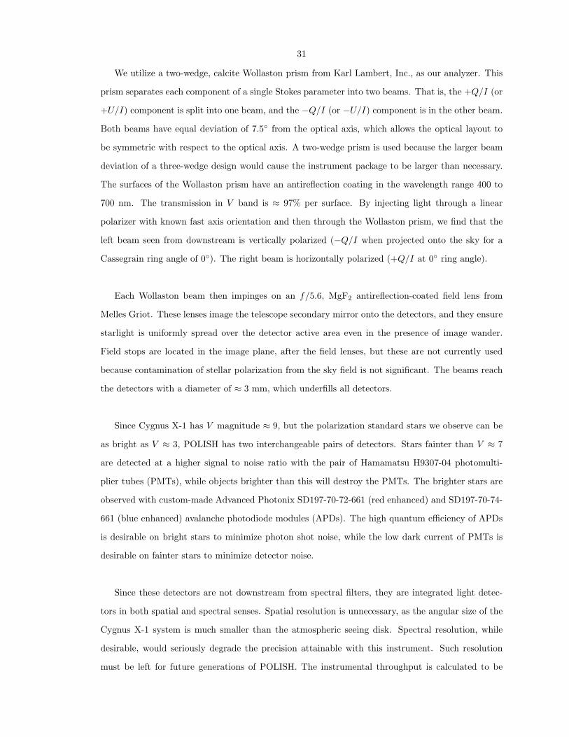
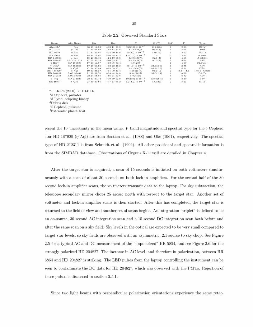
(2000). A list of the stars observed is given in Table 2.2, and polarization values in parenthesis rep-

35

Table 2.2: Observed Standard Stars

Name Alt. Name RA Dec P Θ (◦) Refa V Type

Algenibb γ Peg 00 13 14.23 +15 11 00.9 630(10) × 10−6 118.1(5) 1 2.83 B2IVHD 7927 φ Cas 01 20 04.92 +58 13 53.8 3.232(53)% 94.0(5) 1 5.01 F0IaHD 9270 η Psc 01 31 29.07 +15 20 44.8 60(30) × 10−6 158(14) 1 3.63 G7IIaHR 5854 α Ser 15 44 16.07 +06 25 32.3 4.3(1.0) × 10−6 − 2 2.64 K2IIIb

HD 147084 o Sco 16 20 38.18 −24 10 09.6 3.490(35)% 32.1(3) 1 4.55 A4II/IIIHD 154445 SAO 141513 17 05 32.24 −00 53 31.7 3.420(24)% 90.2(2) 1 5.64 B1V

u Herc HD 156633 17 17 19.57 +33 06 00.4 0.0(2)% − 1 4.80 B1.5Vp+γ Ophd HD 161868 17 47 53.56 +02 42 26.3 80(10) × 10−6 33.3(3.6) 1 3.75 A0V

HD 157999 σ Oph 17 26 30.98 +04 08 25.1 1.010(35)% 85.9(1.0) 1 4.34 K3IabHD 187929e η Aql 19 52 28.37 +01 00 20.4 1.685(3)% 94.2(1) 2 3.5 − 4.3 (F6.5−G2)IbHD 204827 SAO 33461 21 28 57.70 +58 44 24.0 5.44(20)% 59.0(1.1) 1 8.00 O9.5VHD 212311 SAO 34361 22 21 58.55 +56 31 52.8 0.02(5)% − 1 8.12 A0Vζ Peg HD 214923 22 41 27.74 +10 49 52.9 100(30) × 10−6 138.0(8.5) 1 3.40 B8V

HR 8974f γ Cep 23 39 20.85 +77 37 56.2 5.2(2.2) × 10−6 130(25) 2 3.23 K1IV

a1−Heiles (2000), 2−HLB 06bβ Cepheid, pulsatorcβ Lyrid, eclipsing binarydDebris diskeδ Cepheid, pulsatorfExtrasolar planet host

resent the 1σ uncertainty in the mean value. V band magnitude and spectral type for the δ Cepheid

star HD 187929 (η Aql) are from Bastien et al. (1988) and Oke (1961), respectively. The spectral

type of HD 212311 is from Schmidt et al. (1992). All other positional and spectral information is

from the SIMBAD database. Observations of Cygnus X-1 itself are detailed in Chapter 4.

After the target star is acquired, a scan of 15 seconds is initiated on both voltmeters simulta-

neously with a scan of about 30 seconds on both lock-in amplifiers. For the second half of the 30

second lock-in amplifier scans, the voltmeters transmit data to the laptop. For sky subtraction, the

telescope secondary mirror chops 25 arcsec north with respect to the target star. Another set of

voltmeter and lock-in amplifier scans is then started. After this has completed, the target star is

returned to the field of view and another set of scans begins. An integration “triplet” is defined to be

an on-source, 30 second AC integration scan and a 15 second DC integration scan both before and

after the same scan on a sky field. Sky levels in the optical are expected to be very small compared to

target star levels, so sky fields are observed with an asymmetric, 2:1 source to sky chop. See Figure

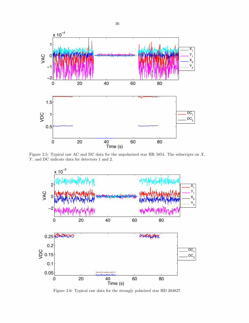
2.5 for a typical AC and DC measurement of the “unpolarized” HR 5854, and see Figure 2.6 for the

strongly polarized HD 204827. The increase in AC level, and therefore in polarization, between HR

5854 and HD 204827 is striking. The LED pulses from the laptop controlling the instrument can be

seen to contaminate the DC data for HD 204827, which was observed with the PMTs. Rejection of

these pulses is discussed in section 2.5.1.

Since two light beams with perpendicular polarization orientations experience the same retar-

36

0 20 40 60 80−2

−1

0

1

x 10−4

VAC

X1Y1X2Y2

0 20 40 60 80

0.5

1

1.5

Time (s)

VDC DC1

DC2

Student Version of MATLAB

Figure 2.5: Typical raw AC and DC data for the unpolarized star HR 5854. The subscripts on X,Y , and DC indicate data for detectors 1 and 2.

0 20 40 60 80

−2

0

2

x 10−3

VAC

X1Y1X2Y2

0 20 40 60 800.05

0.1

0.15

0.2

0.25

Time (s)

VDC DC1

DC2


Figure 2.6: Typical raw data for the strongly polarized star HD 204827.

37

dance when passed through the PEM, the same polarization should be observed for the PEM at

θPEM = ±45◦ with respect to the optical axis of the instrument. We rotate the PEM between these

two positions to investigate the systematics of the PEM. The PEM is mounted to a gear driven

by a stepper motor with an 8:1 step ratio, where the center of the PEM aperture is coincident

with the rotation axis of the gear. Each motor step corresponds to a rotation of the PEM by

∆θPEM = 0.1125◦. For a Cassegrain ring angle of φ = 0◦, the home position of the PEM projects

its compression/extension axis northeast onto the sky (the +U direction). This will be referred to

as the “PEM +45◦” position. The “PEM −45◦” position causes this projection to be northwest on

the sky (the −U direction).

Rotation of a polarized beam follows a cos(2θ) profile, so we rotate the Cassegrain ring and

instrument through ∆φ = 360◦ to investigate the systematics of the rotation. The precision of the

Cassegrain ring angle is 0.1◦. A standard observing sequence begins with the Cassegrain ring at

φ = +180◦ and an integration triplet at the PEM +45◦ position followed by a triplet at the PEM

−45◦ position. The ring angle is then decremented by ∆φ = 45◦, at which point a PEM −45◦ triplet

and PEM +45◦ triplet are taken. This process occurs for each target star for Cassegrain ring angles

of +180◦ > φ > −180◦ in ∆φ = 45◦ increments to sample all ±Q/I and ±U/I Stokes components.

The next star will see the ring angles begin at φ = −180◦ and end at φ = +180◦. The endpoints of

φ = ±180◦ ensure that the ring will not “wind up” and be forced to de-rotate during an observing

sequence, wasting observing time. After each triplet, either the PEM or Cassegrain ring is rotated

but not both. Each standard star is generally given eight Cassegrain ring rotations (∆φ = 360◦) at

two PEM positions each (θPEM = ±45◦), and two chop integrations are taken at each PEM position.

Thus, most standard stars receive about 16 minutes of AC data and about 8 minutes of DC data

per night.

2.5 Data Reduction

2.5.1 Polarization and Noise Calculations

Mean X, Y , and DC values for each detector are found for all on-source and sky scans. The mean

on-source values are then subtracted by the mean sky values. Assuming Stokes Q/I is observed, the

polarization is calculated by the following (Appendix B):

38

Qobs

Iobs=√

2EPEM

√(Xsrc −Xsky)2 + (Ysrc − Ysky)2

DCsrc −DCsky. (2.4)

The efficiency of the PEM, EPEM, is the strength of the AC signal based on the choice of PEM peak

retardance, and it is derived in Appendix B. For POLISH, this efficiency is EPEM ≈ 86%. The sign

of the final polarization of each on-source scan is multiplied by the sign of the Stokes parameter

measured, as given by Table 2.1. That is, the sign of the calculated Stokes parameter is calibrated

by the phase from the lock-in amplifiers (Equation 2.3b).

Expected photon shot noise, detector noise, and observed noise are derived in Appendix C as

Equations C11 and C12a through C12c:

σPshot =γ0

√2

EPEMDC

{1tAC

[BAC +

12

min (Bmax, B) (EPEMP )2

]} 12

(2.5a)

σPdetector =γ√

2EPEMDC

{1tAC

[BAC +

12

min (Bmax, B) (EPEMP )2

]} 12

(2.5b)

σPobs =√

2EPEMDC

{1tAC

[X2σ2

X + Y 2σ2Y

X2 + Y 2+

12

(EPEMPσDC)2

]} 12

(2.5c)

Bmax =(

DCeGTA

) 12

. (2.5d)

Here, γ0 ≡ 2eGTADC, γ ≡ 2eG1+xTA(DC + i′dTA), e is the electron charge, BAC ≈ 2.6 Hz is the

bandwidth of the lock-in amplifiers, and tAC is the integration time of the lock-in amplifiers (Figures

2.5 and 2.6). The values i′d, x, B, G, and TA are the detector’s output dark current, excess noise

factor, bandwidth, gain, and transimpedance, which are listed in Table 2.3. A perfect detector will

have noiseless gain, x = 0, and dark current i′d = 0. Each of the uncertainties σX,Y,DC represents

the sample standard deviation of X, Y , or DC of the source added in quadrature to that of the sky.

The values X, Y , and DC in Equation 2.5c are sky-subtracted.

Short pulses can be seen in the DC data taken with the PMTs (see detector 2 data in Figure

2.6). These pulses have been traced to scattered light from LEDs mounted in the laptop controlling

the instrument. They are easily removed by subtracting off any linear trend in a DC scan and then

39

Table 2.3: Detector Quantities

Detector G x TA B i′d(A/A) (V/A) (kHz) (nA)

Blue APD 300 0.138 4× 106 90 3.5Red APD 220 0.138 4× 106 100 5.6

PMT 5× 106 0.013 105 200 0.1

rejecting data points that lie more than one RMS from the median DC level. The linear trend is

then added back to the DC data before mean and RMS values are computed. The pulses are large

enough that few non-pulse data lie above one RMS from the median. Since the spurious LED signals

are scattered back into the instrument case, they do not pass through the PEM and therefore have

no effect on the AC data.

2.5.2 PEM Calibration

To determine the systematics of the PEM rotation in the lab, we injected pure polarized light into

the instrument by placing a linear polarizer between a green LED and the PEM. We aligned the

polarizer to the Wollaston axis by rotating it until the maximum DC signal was achieved. This

occurs for polarizer angle ψ = 0◦ with respect to the Wollaston axis, as shown in Equation A5.

It might seem that the best way to align the polarizer is by taking the ratio of the AC and DC

signal as in Equation 2.4, but it can be seen from Equation B10 that misalignment of the PEM

from θPEM = ±45◦ will cause misalignment of the polarizer with this technique. Thus, the PEM

was powered down when aligning the polarizer. With the polarizer aligned, Q0/I0 = 99.98% and

U0/I0 = 0.

With the full system turned on, we sampled the polarization as the PEM was swept through the

PEM +45◦ and −45◦ positions. The results are shown in Figure 2.7. The values of ΘPEM are the

expected positions of the rotation motor. For the PEM −45◦ position, the peak polarization lies

almost exactly at ΘPEM = −45◦. Given U0/I0 = 0 above, Equation B10 implies

Qobs

Iobs=Q0

I0

sin2 2θPEM

1 + Q0I0

[cos2 2θPEM + J0 (β0) sin2 2θPEM

] (2.6)

40

−47 −45 −430.508

0.51

0.512

0.514

0.516

0.518

0.52

ΘPEM (°)

Qob

s / I ob

s

(a)

−2 0 24.5

5

5.5

6

6.5

7

7.5

x 10−4

ΘPEM (°)

(b)

43 45 470.508

0.51

0.512

0.514

0.516

0.518

0.52

ΘPEM (°)

(c)


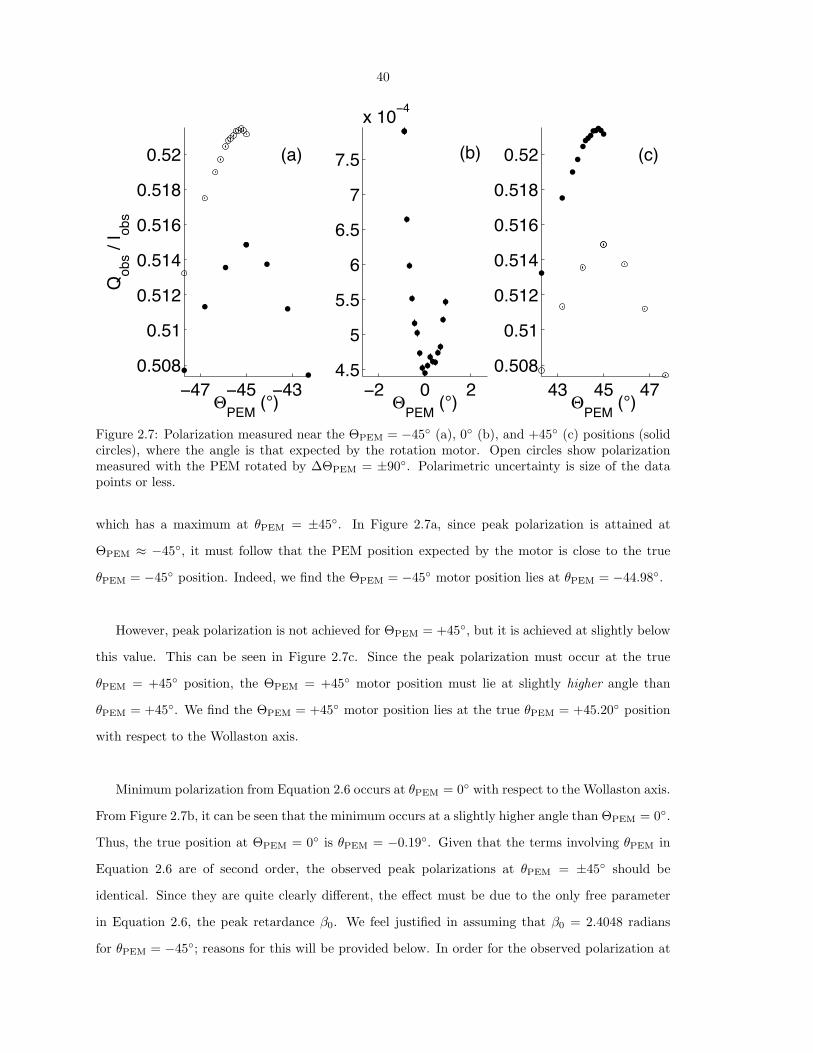
Figure 2.7: Polarization measured near the ΘPEM = −45◦ (a), 0◦ (b), and +45◦ (c) positions (solidcircles), where the angle is that expected by the rotation motor. Open circles show polarizationmeasured with the PEM rotated by ∆ΘPEM = ±90◦. Polarimetric uncertainty is size of the datapoints or less.

which has a maximum at θPEM = ±45◦. In Figure 2.7a, since peak polarization is attained at

ΘPEM ≈ −45◦, it must follow that the PEM position expected by the motor is close to the true

θPEM = −45◦ position. Indeed, we find the ΘPEM = −45◦ motor position lies at θPEM = −44.98◦.

However, peak polarization is not achieved for ΘPEM = +45◦, but it is achieved at slightly below

this value. This can be seen in Figure 2.7c. Since the peak polarization must occur at the true

θPEM = +45◦ position, the ΘPEM = +45◦ motor position must lie at slightly higher angle than

θPEM = +45◦. We find the ΘPEM = +45◦ motor position lies at the true θPEM = +45.20◦ position

with respect to the Wollaston axis.

Minimum polarization from Equation 2.6 occurs at θPEM = 0◦ with respect to the Wollaston axis.

From Figure 2.7b, it can be seen that the minimum occurs at a slightly higher angle than ΘPEM = 0◦.

Thus, the true position at ΘPEM = 0◦ is θPEM = −0.19◦. Given that the terms involving θPEM in

Equation 2.6 are of second order, the observed peak polarizations at θPEM = ±45◦ should be

identical. Since they are quite clearly different, the effect must be due to the only free parameter

in Equation 2.6, the peak retardance β0. We feel justified in assuming that β0 = 2.4048 radians

for θPEM = −45◦; reasons for this will be provided below. In order for the observed polarization at

41

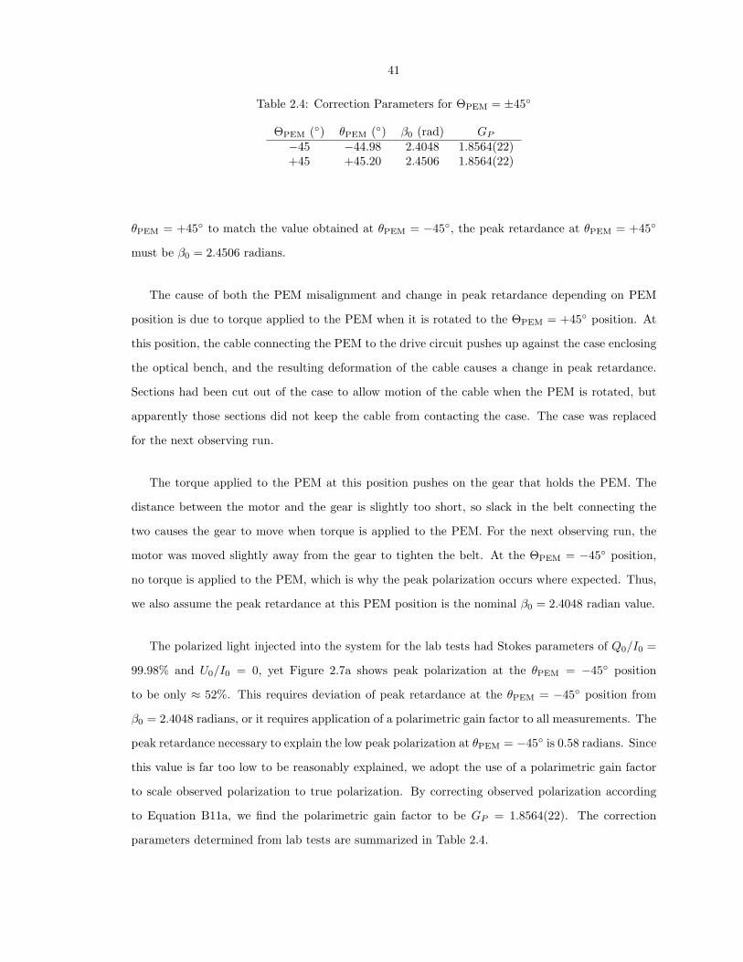
Table 2.4: Correction Parameters for ΘPEM = ±45◦

ΘPEM (◦) θPEM (◦) β0 (rad) GP−45 −44.98 2.4048 1.8564(22)+45 +45.20 2.4506 1.8564(22)

θPEM = +45◦ to match the value obtained at θPEM = −45◦, the peak retardance at θPEM = +45◦

must be β0 = 2.4506 radians.

The cause of both the PEM misalignment and change in peak retardance depending on PEM

position is due to torque applied to the PEM when it is rotated to the ΘPEM = +45◦ position. At

this position, the cable connecting the PEM to the drive circuit pushes up against the case enclosing

the optical bench, and the resulting deformation of the cable causes a change in peak retardance.

Sections had been cut out of the case to allow motion of the cable when the PEM is rotated, but

apparently those sections did not keep the cable from contacting the case. The case was replaced

for the next observing run.

The torque applied to the PEM at this position pushes on the gear that holds the PEM. The

distance between the motor and the gear is slightly too short, so slack in the belt connecting the

two causes the gear to move when torque is applied to the PEM. For the next observing run, the

motor was moved slightly away from the gear to tighten the belt. At the ΘPEM = −45◦ position,

no torque is applied to the PEM, which is why the peak polarization occurs where expected. Thus,

we also assume the peak retardance at this PEM position is the nominal β0 = 2.4048 radian value.

The polarized light injected into the system for the lab tests had Stokes parameters of Q0/I0 =

99.98% and U0/I0 = 0, yet Figure 2.7a shows peak polarization at the θPEM = −45◦ position

to be only ≈ 52%. This requires deviation of peak retardance at the θPEM = −45◦ position from

β0 = 2.4048 radians, or it requires application of a polarimetric gain factor to all measurements. The

peak retardance necessary to explain the low peak polarization at θPEM = −45◦ is 0.58 radians. Since

this value is far too low to be reasonably explained, we adopt the use of a polarimetric gain factor

to scale observed polarization to true polarization. By correcting observed polarization according

to Equation B11a, we find the polarimetric gain factor to be GP = 1.8564(22). The correction

parameters determined from lab tests are summarized in Table 2.4.

42

2.5.3 Mean Polarization

After the polarization from each measurement is corrected for PEM position and peak retardance ac-

cording to Table 2.4, the polarimetric gain factor GP is applied. Since P0 = PobsGP , the polarimetric

uncertainty of each measurement is

σP0 =√

(GPσPobs)2 + (PobsσGP )2

. (2.7)

Telescope polarization is then subtracted, which is discussed in detail in the next section. For each

measurement, the weighted mean polarization from both detectors 1 and 2 is also taken, and the

weight for each detector is the integrated DC level divided by the detector gain. Since the blue

enhanced APD has a higher gain than the red enhanced one by a factor of 1.36, the DC signal from

the blue enhanced APD is expected to be higher than for the red enhanced one. The polarimetric

uncertainty in this combined-detector measurement is taken as the quadrature addition of the po-

larimetric uncertainties from both detectors.

Nightly mean and run-averaged Q0/I0 and U0/I0 for each source are determined by taking the

weighted mean polarization of all corrected data over the requested timescale. The weighting for

each measurement is its sky-subtracted DC level multiplied by integration time. As stated in section

2.5.1, this value is proportional to the total number of detected photons. Weighting by this value

ensures all detected photons, rather than all measurements, are weighted equally. This is important

for data taken in partly cloudy conditions. The polarimetric uncertainty is the square root of the

weighted variance divided by the square root of the number of measurements. It is important to

note that this precision is only applicable to stars with no intrinsic polarimetric variability. Analyses

of the variability of the observed stars, including Cygnus X-1, are made in Chapter 3.

2.6 Standard Stars with APDs

2.6.1 Unpolarized Standard Stars and Systematic Effects

From Table 2.2, the polarizations of both HR 5854 and HR 8974 are close to zero, which makes

them candidates for being truly unpolarized sources. The nightly average polarization of HR 5854

43

and HR 8974, before subtraction of telescope polarization, are listed in Table 2.5 and plotted in

Figures 2.8 and 2.9. For each detector, the weighted mean Stokes parameters for both stars are

generally within one sigma of each other. We therefore assume that these stars are indeed unpolar-

ized and that the combination of telescope and instrumental polarization causes the observed net

polarization of order one part in 104. Since the light beam from the telescope secondary mirror im-

pinges immediately on the PEM, we assume that instrumental polarization is negligible. Indeed, the

very similar setup of PlanetPol has an instrumental polarization of a few parts per million (HLB 06).

The equatorial mount of the Hale 5-m inhibits traditional telescope polarization measurement,

which involves allowing the field to rotate and determining the center of the (Q,U) locus. Since

HLB 06 performed this analysis and claim part per million polarization of HR 5854 and HR 8974,

telescope polarization for the Hale 5-m is thus calculated by the weighted mean polarization from

HR 5854 and HR 8974 (Table 2.6). Uncertainty is given as the square root of the weighted variance

of the individual scans divided by the square root of the number of scans. The cause of the large

telescope polarization of the Hale 5-m is unknown, but it may be due to inhomogeneities in the

coating of the primary and/or secondary mirrors.

The PEM is rotated to positions of θPEM = ±45◦ with respect to the Wollaston axis, and the

Cassegrain ring is rotated through ∆φ = 360◦. This gives independent measures of the PEM and

ring rotation systematics. Note that PlanetPol allows the instrument to be rotated to positions of

±45◦ with respect to their PEM, but this 90◦ rotation of the instrument also causes the Stokes

parameter of opposite sign to be observed. That is, PEM and instrument rotation systematics are

coupled for PlanetPol, while they can be independently measured for POLISH. In addition, Planet-

Pol can measure ±Q/I and ±U/I, but it can only rotate through 135◦. The ∆φ = 360◦ rotation of

POLISH enables more thorough measurement of the instrument rotation systematics.

To investigate the PEM systematics, we must subtract the offset due to ring rotation systematics.

We first find the weighted mean polarization of each Stokes parameter for each star separately, and

at each of the θPEM = ±45◦ positions. We average ring angles φ = 0◦ to φ = 270◦ in ∆φ = 90◦

increments for the Q/I parameter and φ = 45◦ to φ = 315◦ in ∆φ = 90◦ increments for the U/I

parameter. Therefore, the mean polarization at each PEM position contains the same offset due

to ring rotation systematics. The sign of the polarization taken at the θPEM = −45◦ position is

reversed, and the unweighted mean is taken across both Stokes parameters and both PEM posi-

44

03 04 05 06 07−2.8

−2.6

−2.4

−2.2

−2

−1.8x 10−4

UT Date, Aug 2007

Q0 /

I 0

03 04 05 06 07

1.4

1.6

1.8

2

2.2

x 10−4

UT Date, Aug 2007

U 0 / I 0


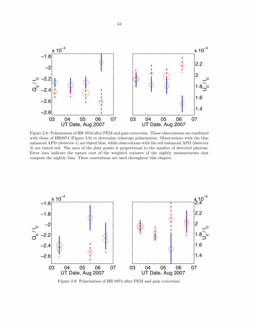
Figure 2.8: Polarization of HR 5854 after PEM and gain correction. These observations are combinedwith those of HR8974 (Figure 2.9) to determine telescope polarization. Observations with the blueenhanced APD (detector 1) are tinted blue, while observations with the red enhanced APD (detector2) are tinted red. The area of the data points is proportional to the number of detected photons.Error bars indicate the square root of the weighted variance of the nightly measurements thatcompose the nightly bins. These conventions are used throughout this chapter.

03 04 05 06 07

−2.6

−2.4

−2.2

−2

−1.8

−1.6x 10−4

UT Date, Aug 2007

Q0 /

I 0

03 04 05 06 07

1.4

1.6

1.8

2

2.2

2.4x 10−4

UT Date, Aug 2007

U 0 / I 0


Figure 2.9: Polarization of HR 8974 after PEM and gain correction.

45

Table 2.5: Raw Polarization of Unpolarized Standard StarsUT Date Star Detector Q0/I0

(×10−6

)U0/I0

(×10−6

)P(×10−6

)Θ (◦)

2007 Aug 3 HR 5854 1 −226.9(2.3) 191.5(3.5) 296.9(2.8) 69.92(29)2007 Aug 4 · · · · · · −231.7(3.3) 182.4(3.8) 294.9(3.5) 70.90(35)2007 Aug 5 · · · · · · −226.9(2.7) 181.0(4.3) 290.2(3.4) 70.71(37)2007 Aug 6 · · · · · · −191.2(4.5) 148.6(4.0) 242.2(4.3) 71.07(50)

Overall · · · · · · −222.9(2.4) 178.0(2.9) 285.2(2.6) 70.70(27)2007 Aug 3 · · · 2 −244.0(3.9) 193.6(4.1) 311.5(4.0) 70.78(37)2007 Aug 4 · · · · · · −241.7(2.8) 203.1(4.4) 315.7(3.5) 69.98(35)2007 Aug 5 · · · · · · −246.1(4.7) 197.4(3.8) 315.5(4.4) 70.63(38)2007 Aug 6 · · · · · · −261.7(5.9) 218.3(4.1) 340.8(5.2) 70.09(41)

Overall · · · · · · −248.1(2.5) 200.4(2.3) 318.9(2.4) 70.54(22)2007 Aug 3 · · · 1,2 −231.6(1.8) 192.2(3.0) 301.0(2.4) 70.16(25)2007 Aug 4 · · · · · · −233.4(2.7) 186.3(3.5) 298.7(3.0) 70.70(31)2007 Aug 5 · · · · · · −236.0(3.0) 189.2(3.3) 302.5(3.1) 70.65(30)2007 Aug 6 · · · · · · −219.9(5.8) 169.6(3.8) 277.7(5.1) 71.17(48)

Overall · · · · · · −231.9(1.8) 185.8(2.0) 297.1(1.9) 70.64(19)2007 Aug 3 HR 8974 1 −239.5(3.8) 195.1(3.0) 308.9(3.5) 70.42(31)2007 Aug 4 · · · · · · −207(25) 174.5(4.0) 271(20) 70.0(1.8)2007 Aug 5 · · · · · · −187.5(6.0) 151.4(8.0) 241.0(6.8) 70.54(86)2007 Aug 6 · · · · · · −221.9(7.2) 205(10) 301.8(8.8) 68.66(85)

Overall · · · · · · −219.6(4.4) 179.9(4.9) 283.8(4.6) 70.34(47)2007 Aug 3 · · · 2 −246.8(3.4) 191.9(3.6) 312.6(3.5) 71.07(32)2007 Aug 4 · · · · · · −199(27) 184.6(4.0) 272(20) 68.6(2.0)2007 Aug 5 · · · · · · −252.5(4.4) 209(10) 327.6(7.3) 70.22(72)2007 Aug 6 · · · · · · −230.8(5.6) 199.5(5.7) 305.0(5.7) 69.58(53)

Overall · · · · · · −243.0(2.9) 197.3(3.4) 313.0(3.1) 70.46(29)2007 Aug 3 · · · 1,2 −240.9(3.2) 194.4(2.2) 309.6(2.9) 70.55(25)2007 Aug 4 · · · · · · −206(37) 177.7(3.4) 272(28) 69.6(2.6)2007 Aug 5 · · · · · · −201.8(6.9) 166.5(5.9) 261.6(6.5) 70.24(69)2007 Aug 6 · · · · · · −224.5(5.6) 202.1(5.3) 302.0(5.5) 69.00(52)

Overall · · · · · · −224.8(3.7) 185.5(2.9) 291.5(3.4) 70.24(32)

tions. The unweighted mean is employed so neither Stokes parameter and neither PEM position

dominates. This value is the PEM offset, given by SPEM (Equation 2.8a). The uncertainty in this

offset is given as one half the difference between the results for Stokes Q and U (Equation 2.8b).

This process is duplicated for each detector and star separately. For the PEM systematic, the index

i represents the PEM position, where i = 0 indicates θPEM = +45◦ and i = 1 indicates θPEM = −45◦.

To investigate the systematics when rotating the Cassegrain ring by 90◦, i.e. the differences

between ±Q or ±U , we subtract the offset due to PEM systematics. While this value has been

calculated above, we prefer to combine the data in such a way as to cause it to cancel. We find

the weighted mean value of each Stokes parameter separately using both θPEM = ±45◦ positions.

We average ring angles φ = 0◦ and φ = 180◦ for the +Q0/I0 parameter, φ = 90◦ and φ = 270◦

46

Table 2.6: Telescope Polarization with APDs

UT Date Detector Q0/I0(×10−6

)U0/I0

(×10−6

)P(×10−6

)Θ (◦)

2007 Aug 3 1 −233.0(2.6) 192.8(2.4) 302.5(2.5) 70.20(23)2007 Aug 4 · · · −230.9(3.3) 181.2(3.3) 293.5(3.3) 70.93(32)2007 Aug 5 · · · −214.8(4.3) 171.9(4.9) 275.1(4.5) 70.66(48)2007 Aug 6 · · · −203.4(5.1) 157.3(6.1) 257.1(5.5) 71.14(64)

Overall · · · −221.8(2.2) 178.5(2.5) 284.7(2.3) 70.59(24)2007 Aug 3 2 −245.1(2.5) 193.1(2.8) 312.1(2.6) 70.88(25)2007 Aug 4 · · · −240.0(3.2) 198.1(3.8) 311.2(3.5) 70.23(33)2007 Aug 5 · · · −246.9(3.5) 198.8(3.7) 317.0(3.5) 70.58(32)2007 Aug 6 · · · −252.5(4.8) 211.8(3.7) 329.5(4.4) 70.00(37)

Overall · · · −247.0(1.9) 199.7(1.9) 317.6(1.9) 70.52(17)2007 Aug 3 1,2 −236.0(2.1) 193.0(2.0) 304.9(2.1) 70.37(19)2007 Aug 4 · · · −232.5(2.8) 184.9(2.8) 297.0(2.8) 70.75(27)2007 Aug 5 · · · −227.5(4.0) 183.6(3.5) 292.3(3.8) 70.55(36)2007 Aug 6 · · · −221.6(4.1) 176.9(3.8) 283.6(4.0) 71.70(40)

Overall · · · −229.8(1.8) 185.7(1.6) 295.5(1.7) 70.53(16)

for −Q0/I0, φ = 45◦ and φ = 225◦ for +U0/I0, and φ = 135◦ and φ = 315◦ for −U0/I0. We then

reverse the signs of the negative Stokes parameters. Taking the unweighted mean for Q0/I0 and

U0/I0 separately, we find the offsets for both Stokes parameters (Equation 2.8a). The uncertainty is

one half the difference between the offsets for the positive and negative Stokes parameters (Equation

2.8b). For the Cassegrain ring systematic, the index i represents the sign of the measured Stokes

parameter, where i = 0 indicates +Q,+U and i = 1 indicates −Q,−U .

SPEM,φ =14

1∑i=0

(−1i

)Qi +

(−1i

)U i (2.8a)

σPEM,φ =14

∣∣∣∣∣1∑i=0

(−1i

)Qi −

(−1i

)U i

∣∣∣∣∣ (2.8b)

In the same way that we found the PEM offset for each Stokes parameter, we now have the

Q0/I0 and U0/I0 offsets for each PEM position. Offsets due to the PEM and ring rotation for HR

5854 and HR 8974 are given in Table 2.7. The “Detector 1,2” value represents systematics obtained

when taking the weighted mean polarization from the simultaneous pairs of measurements from

detector 1 and 2. The “Detector Mean” value represents the mean systematic across the previous

three detector combinations weighted by the inverse square of the uncertainties. This is in contrast

47

Table 2.7: Systematic Effects: Unpolarized Standard Stars with APDs

Star Parameter Detector 1 Detector 2 Detector 1,2 Detector MeanHR 5854 SPEM

(×10−6

)+3.0(1.2) +3.22(19) +2.36(60) +3.14(24)

· · · Sφ(×10−6

)−1.34(13) +0.78(37) −0.2(1.2) −1.11(65)

HR 8974 SPEM

(×10−6

)+4.6(3.2) +2.8(3.1) +3.8(1.8) +3.77(58)

· · · Sφ(×10−6

)−4.5(1.6) −4.9(1.9) −5.44(99) −5.12(40)

to our usual use of weighting by DC level in order to benefit those detectors with good measurement

of systematic effects.

2.6.2 Polarized Standard Stars

We subtract telescope polarization in two ways. The first is by subtracting the nightly telescope

polarization from the nightly stellar polarization, and the second is by subtracting the run-averaged

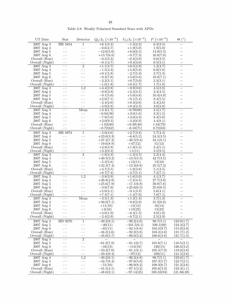
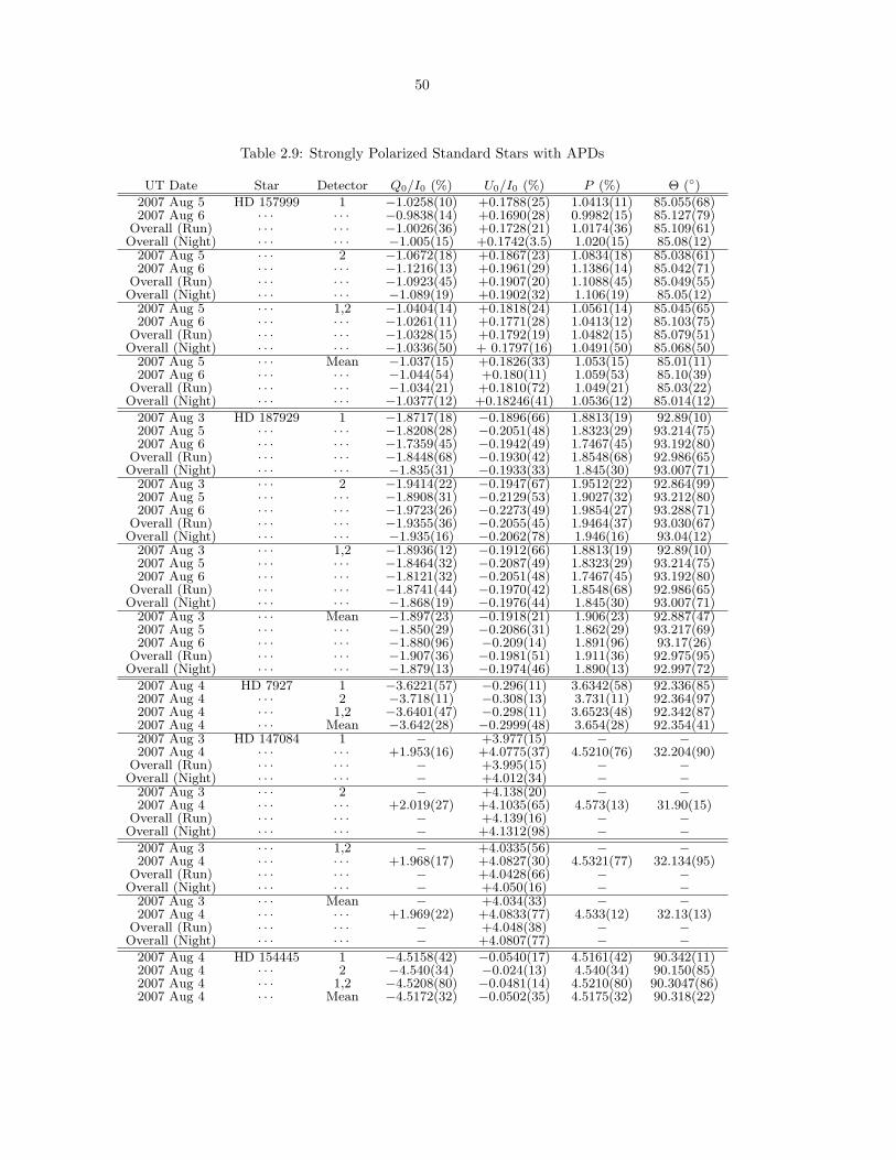
telescope polarization from the nightly stellar polarization. Tables 2.8 and 2.9 list telescope sub-

tracted polarizations for all stars observed with APDs: weakly polarized stars are given in Table

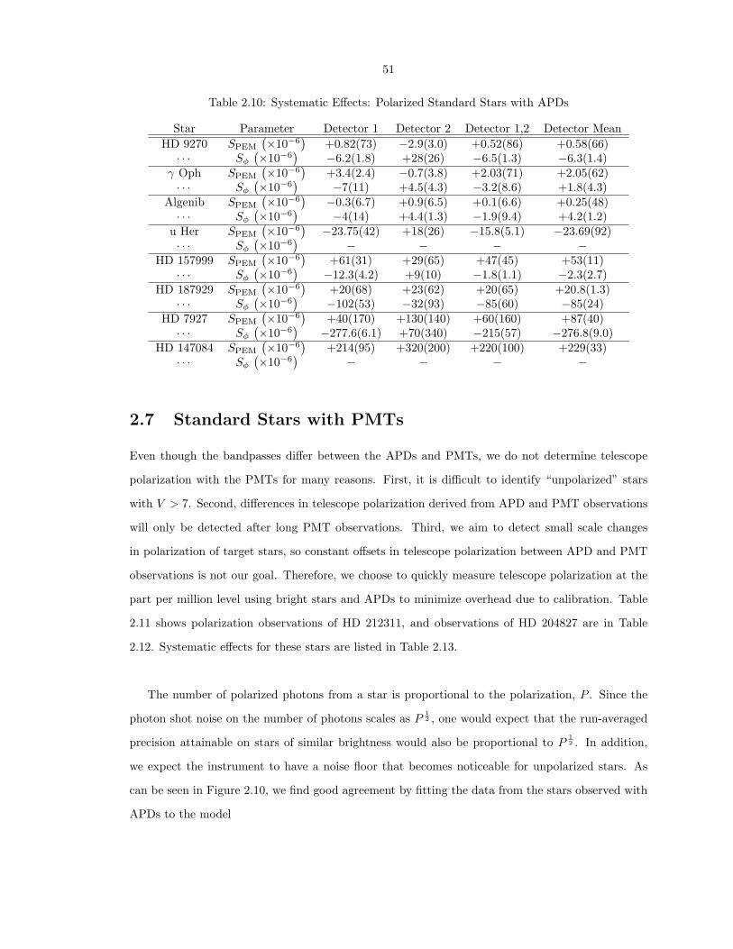
2.8, while strongly polarized stars are listed in Table 2.9. Systematic effects for each star are listed

in Table 2.10. Since HR 5854 and HR 8974 are effectively unpolarized, uncertainty in polarimetric

position angle Θ is so large as to preclude meaningful estimates on Θ.

Due to poor weather, data at only one Cassegrain ring angle and one PEM position were taken

for ζ Peg. The asterisks for this star indicate that, since no measurements for U0/I0 or θPEM = −45◦

exist, the data cannot be calibrated for PEM position and peak retardance. These data have been

subtracted by the telescope polarization, but uncertainty in these measurements is surely large. In-

deed, there is a large difference between subtraction by the telescope polarization obtained during

the single night of ζ Peg observation and by the run-averaged telescope polarization.

48

Table 2.8: Weakly Polarized Standard Stars with APDs

UT Date Star Detector Q0/I0`×10−6

´U0/I0

`×10−6

´P`×10−6

´Θ (◦)

2007 Aug 3 HR 5854 1 +6.1(3.4) −1.3(4.2) 6.3(3.5) −2007 Aug 4 · · · · · · −0.6(4.7) +1.9(5.0) 1.9(5.0) −2007 Aug 5 · · · · · · −12.6(5.0) +8.0(6.5) 14.9(5.5) −2007 Aug 6 · · · · · · +13.7(6.8) −9.7(7.3) 16.8(7.0) −

Overall (Run) · · · · · · −0.5(3.3) −0.4(3.9) 0.6(3.5) −Overall (Night) · · · · · · −0.1(4.7) +0.4(3.0) 0.5(3.1) −

2007 Aug 3 · · · 2 +1.1(4.7) +0.5(4.9) 1.2(4.7) −2007 Aug 4 · · · · · · −1.5(4.3) +5.8(5.8) 6.0(5.8) −2007 Aug 5 · · · · · · +0.1(5.8) −2.7(5.3) 2.7(5.3) −2007 Aug 6 · · · · · · −9.3(7.6) +5.6(5.6) 10.8(7.1) −

Overall (Run) · · · · · · −2.2(3.1) +0.7(3.0) 2.3(3.1) −Overall (Night) · · · · · · −1.6(1.8) +0.3(1.7) 1.7(1.8) −

2007 Aug 3 · · · 1,2 +4.4(2.8) −0.9(3.6) 4.5(2.8) −2007 Aug 4 · · · · · · −0.8(3.9) +2.3(4.5) 2.4(4.5) −2007 Aug 5 · · · · · · −9.1(5.0) +5.0(4.8) 10.4(4.9) −2007 Aug 6 · · · · · · +2.0(7.1) −8.1(5.4) 8.4(5.5) −

Overall (Run) · · · · · · −2.4(2.6) +0.3(2.6) 2.4(2.6) −Overall (Night) · · · · · · −2.0(2.8) +0.4(2.3) 2.0(2.8)

2007 Aug 3 · · · Mean +4.4(1.7) −0.70(68) 4.5(1.7) −2007 Aug 4 · · · · · · −0.94(38) +3.0(1.6) 3.2(1.5) −2007 Aug 5 · · · · · · −7.9(5.0) +3.0(4.3) 8.4(5.0) −2007 Aug 6 · · · · · · +3.0(9.3) −3.2(6.9) 4.4(8.1) −

Overall (Run) · · · · · · −1.82(80) +0.30(40) 1.84(79) −Overall (Night) · · · · · · −0.72(62) −0.10(71) 0.72(63) −

2007 Aug 3 HR 8974 1 −5.0(4.6) +2.7(3.8) 5.7(4.4) −2007 Aug 4 · · · · · · +23.6(3.3) −6.8(5.2) 24.5(3.5) −2007 Aug 5 · · · · · · +27.2(7.3) −20.5(9.4) 34.1(8.1) −2007 Aug 6 · · · · · · −19.6(8.9) +47(12) 51(12) −

Overall (Run) · · · · · · +2.9(4.9) +1.9(5.5) 3.4(5.1) −Overall (Night) · · · · · · +3.2(9.3) +1(11) 3.5(9.5) −

2007 Aug 3 · · · 2 −1.8(4.3) −1.3(4.5) 2.2(4.4) −2007 Aug 4 · · · · · · +40.5(3.2) −13.5(5.5) 42.7(3.5) −2007 Aug 5 · · · · · · −5.3(5.6) +12(11) 13(10) −2007 Aug 6 · · · · · · +22.3(7.4) −12.3(6.8) 25.5(7.2) −

Overall (Run) · · · · · · +4.7(3.5) −1.9(3.8) 5.1(3.5) −Overall (Night) · · · · · · +6.7(7.4) −2.7(5.1) 7.2(7.1) −

2007 Aug 3 · · · 1,2 −3.8(3.9) +1.6(3.0) 4.1(3.7) −2007 Aug 4 · · · · · · +26.8(2.8) −7.2(4.5) 27.7(3.0) −2007 Aug 5 · · · · · · +25.6(7.9) −17.1(6.8) 30.8(7.6) −2007 Aug 6 · · · · · · −3.0(7.0) +25.6(6.5) 25.8(6.5) −

Overall (Run) · · · · · · +5.6(4.1) −0.1(3.3) 5.6(4.1) −Overall (Night) · · · · · · +7.4(7.1) −1.4(7.0) 7.6(7.1) −

2007 Aug 3 · · · Mean −3.5(1.3) +1.3(1.4) 3.7(1.3) −2007 Aug 4 · · · · · · +30.0(7.1) −8.8(2.9) 31.3(6.8) −2007 Aug 5 · · · · · · +11(16) −12(12) 16(14) −2007 Aug 6 · · · · · · +2(16) +13(22) 13(22) −

Overall (Run) · · · · · · +4.6(1.0) −0.4(1.3) 4.6(1.0) −Overall (Night) · · · · · · −2.4(2.9) −0.7(2.1) 2.5(2.9) −

2007 Aug 4 HD 9270 1 −40.2(6.1) −90.2(4.8) 98.7(5.1) 123.0(1.7)2007 Aug 5 · · · · · · −40(11) −101.5(6.1) 109.1(69) 124.3(2.7)2007 Aug 6 · · · · · · −65(11) −82.1(8.8) 104.5(9.7) 115.9(2.8)

Overall (Run) · · · · · · −46.2(4.6) −92.2(3.8) 103.2(4.0) 121.7(1.2)Overall (Night) · · · · · · −45.0(5.7) −90.0(3.2) 100.6(3.8) 121.7(1.5)

2007 Aug 4 · · · 2 − − − −2007 Aug 5 · · · · · · −61.2(7.8) −81.1(6.7) 101.6(7.1) 116.5(2.1)2007 Aug 6 · · · · · · −34(13) −114(16) 120(15) 126.6(3.2)

Overall (Run) · · · · · · −53.3(7.0) −91.1(8.1) 105.5(7.9) 119.8(2.0)Overall (Night) · · · · · · −49.4(9.4) −97(12) 109(11) 121.5(2.6)

2007 Aug 4 · · · 1,2 −40.2(6.1) −90.2(4.8) 98.7(5.1) 123.0(1.7)2007 Aug 5 · · · · · · −44.7(8.4) −97.6(5.0) 107.3(5.7) 122.7(2.1)2007 Aug 6 · · · · · · −51(10) −96.9(8.2) 109.3(8.7) 121.2(2.6)

Overall (Run) · · · · · · −41.5(4.1) −97.1(3.2) 105.6(3.3) 123.4(1.1)Overall (Night) · · · · · · −48.0(2.1) −97.14(25) 108.33(94) 121.86(49)

49

Weakly Polarized Standard Stars with APDs (continued)


´U0/I0

`×10−6

´P`×10−6

´Θ (◦)

2007 Aug 4 HD 9270 Mean −40.2(6.1) −90.2(4.8) 98.7(5.1) 123.0(1.7)2007 Aug 5 · · · · · · −50.5(9.2) −94.6(8.0) 107.2(8.3) 121.0(2.4)2007 Aug 6 · · · · · · −52(12) −93(11) 107(11) 120.5(3.0)

Overall (Run) · · · · · · −45.2(4.2) −94.8(2.6) 105.0(2.9) 122.3(1.1)Overall (Night) · · · · · · −50.94(41) −94.09(49) 106.99(47) 120.78(12)

2007 Aug 4 γ Oph 1 −106.3(8.0) +161.2(6.5) 193.1(7.0) 61.7(1.1)2007 Aug 5 · · · · · · −102.8(7.1) +159.0(8.0) 189.3(7.8) 61.4(1.1)2007 Aug 6 · · · · · · −56(12) +119(12) 132(12) 57.7(2.5)

Overall (Run) · · · · · · −88.5(6.4) +142.5(6.3) 167.7(6.3) 60.9(1.1)Overall (Night) · · · · · · −92(12) +149(10) 176(11) 60.9(1.9)

2007 Aug 4 · · · 2 −87.6(7.5) +158.9(8.1) 181.5(8.0) 59.4(1.2)2007 Aug 5 · · · · · · −87.3(6.4) +164.5(8.3) 186.2(7.9) 59.0(1.1)2007 Aug 6 · · · · · · −116(11) +176.0(9.2) 210.8(9.8) 61.7(1.4)

Overall (Run) · · · · · · −95.3(5.1) +169.4(5.1) 194.4(5.1) 59.68(75)Overall (Night) · · · · · · −95.1(7.4) +166.8(3.5) 192.0(4.7) 59.85(99)

2007 Aug 4 · · · 1,2 −102.7(6.7) +160.2(5.1) 190.3(5.6) 61.33(94)2007 Aug 5 · · · · · · −97.3(4.7) +162.5(5.8) 189.4(5.6) 60.45(76)2007 Aug 6 · · · · · · −78.1(9.1) +140.7(8.4) 160.9(8.6) 59.5(1.6)

Overall (Run) · · · · · · −92.1(4.1) +152.5(4.0) 178.2(4.0) 60.56(65)Overall (Night) · · · · · · −94.2(5.6) +156.1(5.3) 182.3(5.4) 60.55(86)

2007 Aug 4 · · · Mean −98.9(7.9) +160.26(78) 188.3(4.2) 60.8(1.0)2007 Aug 5 · · · · · · −95.7(5.7) +162.1(2.0) 188.2(3.4) 60.28(76)2007 Aug 6 · · · · · · −83(23) +148(22) 170(22) 59.7(3.8)

Overall (Run) · · · · · · −92.4(2.4) +155.6(9.8) 181.0(8.5) 60.34(86)Overall (Night) · · · · · · −96.3(1.7) +160.49(42) 187.16(96) 60.48(23)

2007 Aug 4 ζ Peg 1 +2(−)* − >2(−)* −2007 Aug 4 · · · 2 +15(−)* − >15(−)* −2007 Aug 4 · · · 1,2 +5(−)* − > 5(−)* −2007 Aug 4 · · · Mean +7(−)* − >7(−)* −2007 Aug 5 Algenib 1 −565(19) −623(19) 841(19) 113.91(64)2007 Aug 6 · · · · · · −702(11) −589(11) 917(11) 109.99(34)

Overall (Run) · · · · · · −646(14) −613.9(9.0) 891(12) 111.78(37)Overall (Night) · · · · · · −658(46) −600(11) 934(13) 111.17(36)

2007 Aug 5 · · · 2 −730.0(6.4) −628.6(7.9) 963.4(7.1) 110.37(22)2007 Aug 6 · · · · · · −668.3(7.9) −643.6(7.1) 927.8(7.5) 111.96(23)

Overall (Run) · · · · · · −698.2(6.3) −630.2(4.9) 940.6(5.7) 111.03(17)Overall (Night) · · · · · · −697(22) −636.6(5.3) 934(13) 111.17(36)

2007 Aug 5 · · · 1,2 −625(12) −627(13) 885(13) 112.54(41)2007 Aug 6 · · · · · · −687.7(8.7) −608.7(8.5) 918.4(8.6) 110.76(27)

Overall (Run) · · · · · · −661.5(8.1) −619.5(6.9) 906.3(7.6) 111.56(24)Overall (Night) · · · · · · −666(21) −615.0(6.1) 907(16) 111.36(47)

2007 Aug 5 · · · Mean −696(57) −627.6(1.7) 937(42) 111.0(1.2)2007 Aug 6 · · · · · · −683(13) −621(22) 923(18) 111.15(58)

Overall (Run) · · · · · · −680(20) −624.5(6.6) 923(16) 111.29(46)Overall (Night) · · · · · · −683.3(2.2) −627.60(36) 927.8(1.6) 111.284(47)

2007 Aug 4 u Her 1 +1547(20) −440(12) 1609(19) 172.06(22)2007 Aug 4 · · · 2 +1585(19) −497(30) 1661(20) 171.30(50)2007 Aug 4 · · · 1,2 +1554(15) −451.5(9.6) 1618(15) 171.90(18)2007 Aug 4 · · · Mean +1561(16) −450(13) 1625(15) 171.97(23)

50

Table 2.9: Strongly Polarized Standard Stars with APDs

UT Date Star Detector Q0/I0 (%) U0/I0 (%) P (%) Θ (◦)

2007 Aug 5 HD 157999 1 −1.0258(10) +0.1788(25) 1.0413(11) 85.055(68)2007 Aug 6 · · · · · · −0.9838(14) +0.1690(28) 0.9982(15) 85.127(79)

Overall (Run) · · · · · · −1.0026(36) +0.1728(21) 1.0174(36) 85.109(61)Overall (Night) · · · · · · −1.005(15) +0.1742(3.5) 1.020(15) 85.08(12)

2007 Aug 5 · · · 2 −1.0672(18) +0.1867(23) 1.0834(18) 85.038(61)2007 Aug 6 · · · · · · −1.1216(13) +0.1961(29) 1.1386(14) 85.042(71)

Overall (Run) · · · · · · −1.0923(45) +0.1907(20) 1.1088(45) 85.049(55)Overall (Night) · · · · · · −1.089(19) +0.1902(32) 1.106(19) 85.05(12)

2007 Aug 5 · · · 1,2 −1.0404(14) +0.1818(24) 1.0561(14) 85.045(65)2007 Aug 6 · · · · · · −1.0261(11) +0.1771(28) 1.0413(12) 85.103(75)

Overall (Run) · · · · · · −1.0328(15) +0.1792(19) 1.0482(15) 85.079(51)Overall (Night) · · · · · · −1.0336(50) + 0.1797(16) 1.0491(50) 85.068(50)

2007 Aug 5 · · · Mean −1.037(15) +0.1826(33) 1.053(15) 85.01(11)2007 Aug 6 · · · · · · −1.044(54) +0.180(11) 1.059(53) 85.10(39)


2007 Aug 3 HD 187929 1 −1.8717(18) −0.1896(66) 1.8813(19) 92.89(10)2007 Aug 5 · · · · · · −1.8208(28) −0.2051(48) 1.8323(29) 93.214(75)2007 Aug 6 · · · · · · −1.7359(45) −0.1942(49) 1.7467(45) 93.192(80)

Overall (Run) · · · · · · −1.8448(68) −0.1930(42) 1.8548(68) 92.986(65)Overall (Night) · · · · · · −1.835(31) −0.1933(33) 1.845(30) 93.007(71)

2007 Aug 3 · · · 2 −1.9414(22) −0.1947(67) 1.9512(22) 92.864(99)2007 Aug 5 · · · · · · −1.8908(31) −0.2129(53) 1.9027(32) 93.212(80)2007 Aug 6 · · · · · · −1.9723(26) −0.2273(49) 1.9854(27) 93.288(71)


2007 Aug 3 · · · 1,2 −1.8936(12) −0.1912(66) 1.8813(19) 92.89(10)2007 Aug 5 · · · · · · −1.8464(32) −0.2087(49) 1.8323(29) 93.214(75)2007 Aug 6 · · · · · · −1.8121(32) −0.2051(48) 1.7467(45) 93.192(80)


2007 Aug 3 · · · Mean −1.897(23) −0.1918(21) 1.906(23) 92.887(47)2007 Aug 5 · · · · · · −1.850(29) −0.2086(31) 1.862(29) 93.217(69)2007 Aug 6 · · · · · · −1.880(96) −0.209(14) 1.891(96) 93.17(26)


2007 Aug 4 HD 7927 1 −3.6221(57) −0.296(11) 3.6342(58) 92.336(85)2007 Aug 4 · · · 2 −3.718(11) −0.308(13) 3.731(11) 92.364(97)2007 Aug 4 · · · 1,2 −3.6401(47) −0.298(11) 3.6523(48) 92.342(87)2007 Aug 4 · · · Mean −3.642(28) −0.2999(48) 3.654(28) 92.354(41)2007 Aug 3 HD 147084 1 − +3.977(15) − −2007 Aug 4 · · · · · · +1.953(16) +4.0775(37) 4.5210(76) 32.204(90)

Overall (Run) · · · · · · − +3.995(15) − −Overall (Night) · · · · · · − +4.012(34) − −

2007 Aug 3 · · · 2 − +4.138(20) − −2007 Aug 4 · · · · · · +2.019(27) +4.1035(65) 4.573(13) 31.90(15)


2007 Aug 3 · · · 1,2 − +4.0335(56) − −2007 Aug 4 · · · · · · +1.968(17) +4.0827(30) 4.5321(77) 32.134(95)


2007 Aug 3 · · · Mean − +4.034(33) − −2007 Aug 4 · · · · · · +1.969(22) +4.0833(77) 4.533(12) 32.13(13)


2007 Aug 4 HD 154445 1 −4.5158(42) −0.0540(17) 4.5161(42) 90.342(11)2007 Aug 4 · · · 2 −4.540(34) −0.024(13) 4.540(34) 90.150(85)2007 Aug 4 · · · 1,2 −4.5208(80) −0.0481(14) 4.5210(80) 90.3047(86)2007 Aug 4 · · · Mean −4.5172(32) −0.0502(35) 4.5175(32) 90.318(22)

51

Table 2.10: Systematic Effects: Polarized Standard Stars with APDs

Star Parameter Detector 1 Detector 2 Detector 1,2 Detector MeanHD 9270 SPEM

(×10−6

)+0.82(73) −2.9(3.0) +0.52(86) +0.58(66)

· · · Sφ(×10−6

)−6.2(1.8) +28(26) −6.5(1.3) −6.3(1.4)

γ Oph SPEM

(×10−6

)+3.4(2.4) −0.7(3.8) +2.03(71) +2.05(62)

· · · Sφ(×10−6

)−7(11) +4.5(4.3) −3.2(8.6) +1.8(4.3)

Algenib SPEM

(×10−6

)−0.3(6.7) +0.9(6.5) +0.1(6.6) +0.25(48)

· · · Sφ(×10−6

)−4(14) +4.4(1.3) −1.9(9.4) +4.2(1.2)

u Her SPEM

(×10−6

)−23.75(42) +18(26) −15.8(5.1) −23.69(92)

· · · Sφ(×10−6

)− − − −

HD 157999 SPEM

(×10−6

)+61(31) +29(65) +47(45) +53(11)

· · · Sφ(×10−6

)−12.3(4.2) +9(10) −1.8(1.1) −2.3(2.7)

HD 187929 SPEM

(×10−6

)+20(68) +23(62) +20(65) +20.8(1.3)

· · · Sφ(×10−6

)−102(53) −32(93) −85(60) −85(24)

HD 7927 SPEM

(×10−6

)+40(170) +130(140) +60(160) +87(40)

· · · Sφ(×10−6

)−277.6(6.1) +70(340) −215(57) −276.8(9.0)

HD 147084 SPEM

(×10−6

)+214(95) +320(200) +220(100) +229(33)

· · · Sφ(×10−6

)− − − −

2.7 Standard Stars with PMTs

Even though the bandpasses differ between the APDs and PMTs, we do not determine telescope

polarization with the PMTs for many reasons. First, it is difficult to identify “unpolarized” stars

with V > 7. Second, differences in telescope polarization derived from APD and PMT observations

will only be detected after long PMT observations. Third, we aim to detect small scale changes

in polarization of target stars, so constant offsets in telescope polarization between APD and PMT

observations is not our goal. Therefore, we choose to quickly measure telescope polarization at the

part per million level using bright stars and APDs to minimize overhead due to calibration. Table

2.11 shows polarization observations of HD 212311, and observations of HD 204827 are in Table

2.12. Systematic effects for these stars are listed in Table 2.13.

The number of polarized photons from a star is proportional to the polarization, P . Since the

photon shot noise on the number of photons scales as P12 , one would expect that the run-averaged

precision attainable on stars of similar brightness would also be proportional to P12 . In addition,

we expect the instrument to have a noise floor that becomes noticeable for unpolarized stars. As

can be seen in Figure 2.10, we find good agreement by fitting the data from the stars observed with

APDs to the model

52

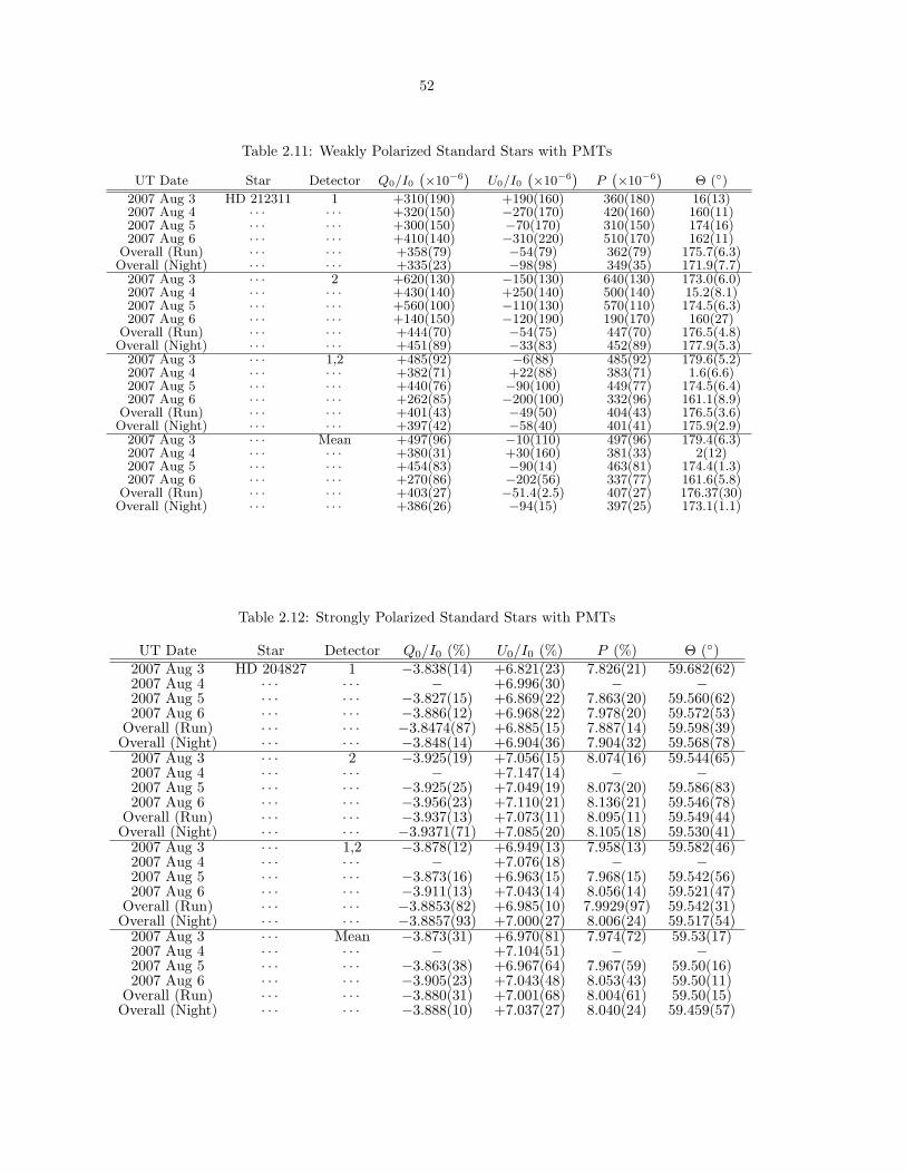
Table 2.11: Weakly Polarized Standard Stars with PMTs


´U0/I0

`×10−6

´P`×10−6

´Θ (◦)

2007 Aug 3 HD 212311 1 +310(190) +190(160) 360(180) 16(13)2007 Aug 4 · · · · · · +320(150) −270(170) 420(160) 160(11)2007 Aug 5 · · · · · · +300(150) −70(170) 310(150) 174(16)2007 Aug 6 · · · · · · +410(140) −310(220) 510(170) 162(11)

Overall (Run) · · · · · · +358(79) −54(79) 362(79) 175.7(6.3)Overall (Night) · · · · · · +335(23) −98(98) 349(35) 171.9(7.7)

2007 Aug 3 · · · 2 +620(130) −150(130) 640(130) 173.0(6.0)2007 Aug 4 · · · · · · +430(140) +250(140) 500(140) 15.2(8.1)2007 Aug 5 · · · · · · +560(100) −110(130) 570(110) 174.5(6.3)2007 Aug 6 · · · · · · +140(150) −120(190) 190(170) 160(27)


2007 Aug 3 · · · 1,2 +485(92) −6(88) 485(92) 179.6(5.2)2007 Aug 4 · · · · · · +382(71) +22(88) 383(71) 1.6(6.6)2007 Aug 5 · · · · · · +440(76) −90(100) 449(77) 174.5(6.4)2007 Aug 6 · · · · · · +262(85) −200(100) 332(96) 161.1(8.9)


2007 Aug 3 · · · Mean +497(96) −10(110) 497(96) 179.4(6.3)2007 Aug 4 · · · · · · +380(31) +30(160) 381(33) 2(12)2007 Aug 5 · · · · · · +454(83) −90(14) 463(81) 174.4(1.3)2007 Aug 6 · · · · · · +270(86) −202(56) 337(77) 161.6(5.8)

Overall (Run) · · · · · · +403(27) −51.4(2.5) 407(27) 176.37(30)Overall (Night) · · · · · · +386(26) −94(15) 397(25) 173.1(1.1)

Table 2.12: Strongly Polarized Standard Stars with PMTs

UT Date Star Detector Q0/I0 (%) U0/I0 (%) P (%) Θ (◦)2007 Aug 3 HD 204827 1 −3.838(14) +6.821(23) 7.826(21) 59.682(62)2007 Aug 4 · · · · · · − +6.996(30) − −2007 Aug 5 · · · · · · −3.827(15) +6.869(22) 7.863(20) 59.560(62)2007 Aug 6 · · · · · · −3.886(12) +6.968(22) 7.978(20) 59.572(53)


2007 Aug 3 · · · 2 −3.925(19) +7.056(15) 8.074(16) 59.544(65)2007 Aug 4 · · · · · · − +7.147(14) − −2007 Aug 5 · · · · · · −3.925(25) +7.049(19) 8.073(20) 59.586(83)2007 Aug 6 · · · · · · −3.956(23) +7.110(21) 8.136(21) 59.546(78)


2007 Aug 3 · · · 1,2 −3.878(12) +6.949(13) 7.958(13) 59.582(46)2007 Aug 4 · · · · · · − +7.076(18) − −2007 Aug 5 · · · · · · −3.873(16) +6.963(15) 7.968(15) 59.542(56)2007 Aug 6 · · · · · · −3.911(13) +7.043(14) 8.056(14) 59.521(47)


2007 Aug 3 · · · Mean −3.873(31) +6.970(81) 7.974(72) 59.53(17)2007 Aug 4 · · · · · · − +7.104(51) − −2007 Aug 5 · · · · · · −3.863(38) +6.967(64) 7.967(59) 59.50(16)2007 Aug 6 · · · · · · −3.905(23) +7.043(48) 8.053(43) 59.50(11)


53

Table 2.13: Systematic Effects: Standard Stars with PMTs

Star Parameter Detector 1 Detector 2 Detector 1,2 Detector MeanHD 212311 SPEM

(×10−6

)−95(74) −32(61) −58(57) −58(37)

· · · Sφ(×10−6

)−65(59) +24(30) −15(45) 0(32)

HD 204827 SPEM

(×10−6

)+540(180) +550(340) +487(36) +490(12)

· · · Sφ(×10−6

)−269(28) +320(210) +30(110) −240(100)

σP =

(P 12

a

)2

+ σ2P0

12

. (2.9)

Here, a is a scaling factor and σP0 is the noise floor of the instrument, which is added in quadrature

to the photon shot noise component. This noise floor appears to be eight parts in ten million. The

fitting was performed using a least-squares approach. However, since the data span five orders of

magnitude in polarization, the residuals to be minimized are given by

SSE =∑i

(σPi − σPσPi

)2

. (2.10)

The stars observed with APDs are all roughly the same visual magnitude. However, the preci-

sion achieved on the weakly polarized HD 212311, observed with PMTs, is worse than for the stars

observed with APDs. HD 212311 is roughly 5 magnitudes fainter than its bright counterparts (Table

2.2), so the precision is expected to be(100.4×5

) 12 = 10 times worse, as observed. Thus, the scaling

factor determined for the APD stars, a, will be an order of magnitude different from the scaling

factor for the PMT stars. This is why the PMT stars were excluded from the above fit. However,

precision on the strongly polarized HD 204827 is surprisingly consistent with the slope for the bright

stars. This is most likely due to the larger dataset obtained on HD 204827.

2.8 Comparison to Literature

2.8.1 Unpolarized Standard Stars

Individual measurements and nightly mean polarization for most stars are shown in Figures 2.11

to 2.30. Those that are not displayed generally have only one night of observations. We compare

54

10−6 10−5 10−4 10−3 10−2 10−1 10010−7

10−6

10−5

10−4

10−3

P

σP APD Stars

PMT Stars


Figure 2.10: Run-averaged precision as a function of stellar polarization. Photon shot noise consider-ations predict precision proportional to the square root of polarization, which is observed. The solidline is a fit to the data with power law slope 1/2 plus the quadrature addition of an instrumentalnoise floor, while the dashed line is the P

12 term.

our results to the polarization catalog of Heiles (2000) and to HLB 06 in Figure 2.31. To determine

polarization for each star, Heiles (2000) take the weighted mean polarization from different authors.

The weights are the inverse square of the uncertainties from each author. Uncertainty in stellar po-

larization in Heiles (2000) is the square root of the sum of squares of residuals between each author’s

polarization and the Heiles (2000) mean polarization.

Uncertainty in degree of polarization is listed nightly for strongly polarized stars in Table 3 of

HLB 06 (HD 7927, HD 147084, HD 154445, and HD 187929). To determine run-averaged uncertainty

for these stars, we first convert their degree, position angle, and uncertainties to Q/I, U/I, and asso-

ciated uncertainties. We then perform a weighted mean for each Stokes parameter separately, where

the weights are the inverse square of the nightly uncertainties in those parameters. Since degree of

polarization is defined to be a positive quantity, taking the mean degree of polarization from the

ensemble of nights would be incorrect.

The degree of polarization measured by POLISH is plotted as open stars, and stellar polarization

increases toward the bottom of the plot. Our precision in the degree of polarization is plotted as

55

filled black circles, precision values computed from HLB 06 are light grey diamonds, and Heiles

(2000) precision values are dark grey squares. The horizontal line before the second star from the

bottom in Figure 2.31 separates those stars observed with APDs (at the top) from those observed

with PMTs (at the bottom).

The rightmost column of the figure shows the position angle of net polarization, where north is

at the top and east is at the left of the plots. Black lines indicate position angle measured with

POLISH, HLB 06 position angles are light grey lines, and Heiles (2000) position angles are dark grey

lines. Agreement between the data sets for stars with low polarization is of course poor, because

position angle of net polarization is meaningless for these stars. As stellar polarization increases,

agreement in position angle also increases. Since agreement between our measurements and the

literature regarding degree of polarization is not our primary objective, accuracy in our observations

is assessed by agreement in position angle of polarization.

The unpolarized standard stars observed in order to determine telescope polarization, HR 5854

(α Ser, HD 140573) and HR 8974 (γ Cep, HD 222404), have run-averaged polarimetric precision

of one part per million or better. This was our precision goal for bright, unpolarized stars. The

precision achieved by PlanetPol on these stars is comparable to our results. However, we have im-

proved the precision on these stars by three orders of magnitude with respect to the Heiles (2000)

catalog. HR 8974 is known to harbor an extrasolar planet with a minimum mass of 1.60 ± 0.13

Jupiter masses, a period of 902.9± 3.5 days, and a semimajor axis of 2.044± 0.057 AU (Neuhauser

et al. 2006). We expect the amplitude of the planetary polarimetric signal to be of order 10−8 or

less and consequently undetectable.

2.8.2 Weakly Polarized Standard Stars

We have improved the polarimetric precision achieved on HD 9270 (η Psc) by an order of magnitude

with respect to Heiles (2000). Precision on γ Oph (HD 161868) and Algenib (γ Peg, HD 886),

however, is only slightly better than tabulated in Heiles (2000). It is expected that longer integration

on these stars will improve this precision. Finally, the precision achieved on u Her (SAO 65913)

has been improved by two orders of magnitude from Heiles (2000). There is an order of magnitude

improvement in precision on HD 212311 with respect to Heiles (2000).

56

03 04 05 06 07−3

−2

−1

0

1

2

x 10−5

UT Date, Aug 2007

Q0 /

I 0

03 04 05 06 07

−2

0

2

x 10−5

UT Date, Aug 2007

U 0 / I 0


Figure 2.11: Nightly mean polarization of the unpolarized star HR 5854. This star was observedwith APDs, and the data are plotted after calibration of the PEM position, peak retardance, gain,and telescope polarization. Solid blue lines indicate observations by the blue enhanced APD1, whiledotted red lines are observed with the red enhanced APD2.

Figure 2.12: Intra-night observations of HR 5854 with APD1, UT 2007 Aug 3 and 4. Observednoise calculated from fluctuations in AC and DC levels is given by error bars on individual datapoints (Figure 2.5 and Equation 2.5c). Area of data points is proportional to the number of detectedphotons. Theoretical detector noise (Equation C11) is given as vertical lines outside the plot boxes,while theoretical photon shot noise (Equation 2.5a) is represented by dashed vertical lines outsidethe plot boxes. These conventions are used throughout this chapter.

57

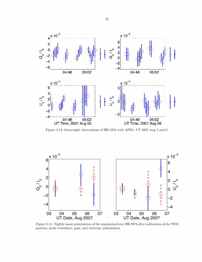
Figure 2.13: Intra-night observations of HR 5854 with APD1, UT 2007 Aug 5 and 6.

03 04 05 06 07

−4

−2

0

2

4

6x 10−5

UT Date, Aug 2007

Q0 /

I 0

03 04 05 06 07−4

−2

0

2

4

6x 10−5

UT Date, Aug 2007

U 0 / I 0


Figure 2.14: Nightly mean polarization of the unpolarized star HR 8974 after calibration of the PEMposition, peak retardance, gain, and telescope polarization.

58

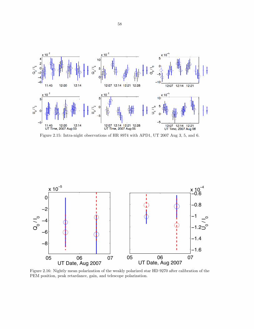
Figure 2.15: Intra-night observations of HR 8974 with APD1, UT 2007 Aug 3, 5, and 6.

05 06 07

−8

−6

−4

−2

0x 10−5

UT Date, Aug 2007

Q0 /

I 0

05 06 07−1.6

−1.4

−1.2

−1

−0.8

−0.6x 10−4

UT Date, Aug 2007

U 0 / I 0


Figure 2.16: Nightly mean polarization of the weakly polarized star HD 9270 after calibration of thePEM position, peak retardance, gain, and telescope polarization.

59

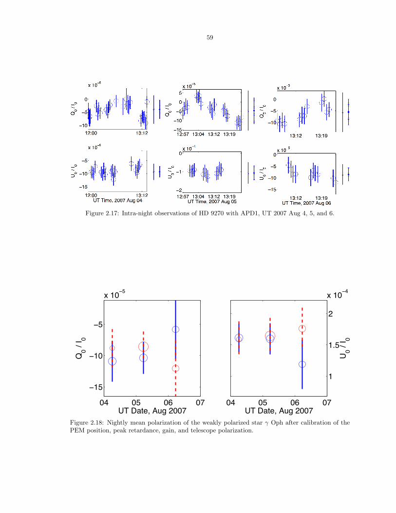
Figure 2.17: Intra-night observations of HD 9270 with APD1, UT 2007 Aug 4, 5, and 6.

04 05 06 07

−15

−10

−5

x 10−5

UT Date, Aug 2007

Q0 /

I 0

04 05 06 07

1

1.5

2

x 10−4

UT Date, Aug 2007

U 0 / I 0


Figure 2.18: Nightly mean polarization of the weakly polarized star γ Oph after calibration of thePEM position, peak retardance, gain, and telescope polarization.

60

Figure 2.19: Intra-night observations of γ Oph with APD1, UT 2007 Aug 4, 5, and 6.

05 06 07−7.5

−7

−6.5

−6

−5.5

−5x 10−4

UT Date, Aug 2007

Q0 /

I 0

05 06 07−7.5

−7

−6.5

−6

−5.5

−5x 10−4

UT Date, Aug 2007

U 0 / I 0


Figure 2.20: Nightly mean polarization of the weakly polarized star Algenib after calibration of thePEM position, peak retardance, gain, and telescope polarization.

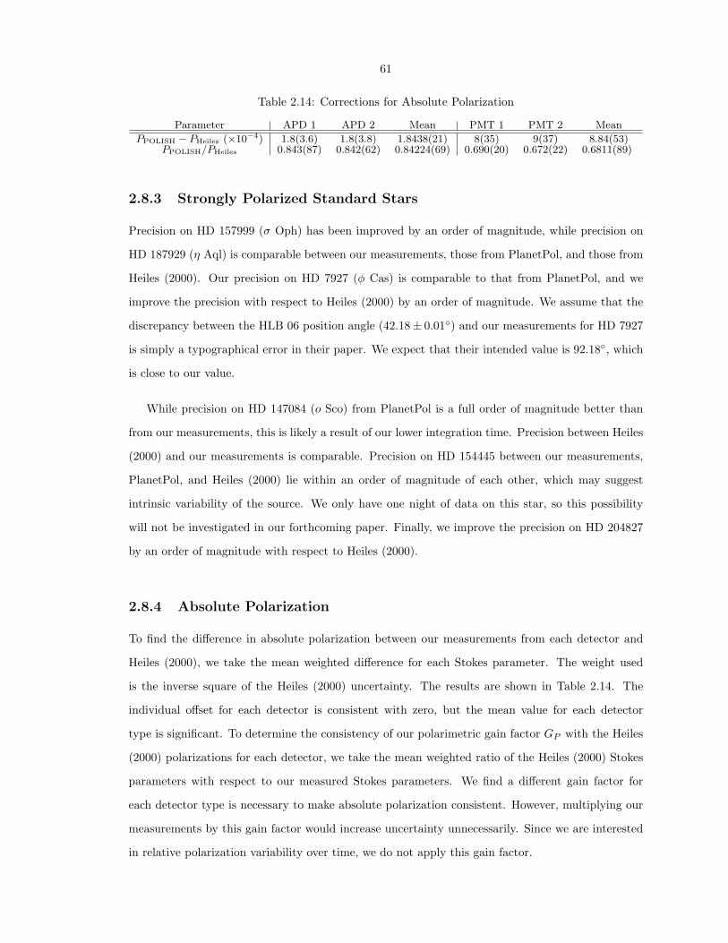
61

Table 2.14: Corrections for Absolute Polarization

Parameter APD 1 APD 2 Mean PMT 1 PMT 2 Mean

PPOLISH − PHeiles (×10−4) 1.8(3.6) 1.8(3.8) 1.8438(21) 8(35) 9(37) 8.84(53)PPOLISH/PHeiles 0.843(87) 0.842(62) 0.84224(69) 0.690(20) 0.672(22) 0.6811(89)

2.8.3 Strongly Polarized Standard Stars

Precision on HD 157999 (σ Oph) has been improved by an order of magnitude, while precision on

HD 187929 (η Aql) is comparable between our measurements, those from PlanetPol, and those from

Heiles (2000). Our precision on HD 7927 (φ Cas) is comparable to that from PlanetPol, and we

improve the precision with respect to Heiles (2000) by an order of magnitude. We assume that the

discrepancy between the HLB 06 position angle (42.18± 0.01◦) and our measurements for HD 7927

is simply a typographical error in their paper. We expect that their intended value is 92.18◦, which

is close to our value.

While precision on HD 147084 (o Sco) from PlanetPol is a full order of magnitude better than

from our measurements, this is likely a result of our lower integration time. Precision between Heiles

(2000) and our measurements is comparable. Precision on HD 154445 between our measurements,

PlanetPol, and Heiles (2000) lie within an order of magnitude of each other, which may suggest

intrinsic variability of the source. We only have one night of data on this star, so this possibility

will not be investigated in our forthcoming paper. Finally, we improve the precision on HD 204827

by an order of magnitude with respect to Heiles (2000).

2.8.4 Absolute Polarization

To find the difference in absolute polarization between our measurements from each detector and

Heiles (2000), we take the mean weighted difference for each Stokes parameter. The weight used

is the inverse square of the Heiles (2000) uncertainty. The results are shown in Table 2.14. The

individual offset for each detector is consistent with zero, but the mean value for each detector

type is significant. To determine the consistency of our polarimetric gain factor GP with the Heiles

(2000) polarizations for each detector, we take the mean weighted ratio of the Heiles (2000) Stokes

parameters with respect to our measured Stokes parameters. We find a different gain factor for

each detector type is necessary to make absolute polarization consistent. However, multiplying our

measurements by this gain factor would increase uncertainty unnecessarily. Since we are interested

in relative polarization variability over time, we do not apply this gain factor.

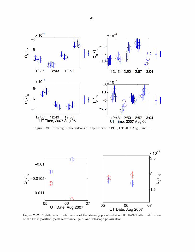
62

Figure 2.21: Intra-night observations of Algenib with APD1, UT 2007 Aug 5 and 6.

05 06 07

−0.011

−0.0105

−0.01

UT Date, Aug 2007

Q0 /

I 0

05 06 07

1.5

2

2.5x 10−3

UT Date, Aug 2007

U 0 / I 0


Figure 2.22: Nightly mean polarization of the strongly polarized star HD 157999 after calibrationof the PEM position, peak retardance, gain, and telescope polarization.

63

Figure 2.23: Intra-night observations of HD 157999 with APD1, UT 2007 Aug 5 and 6.

03 04 05 06 07

−0.0195

−0.019

−0.0185

−0.018

−0.0175

UT Date, Aug 2007

Q0 /

I 0

03 04 05 06 07

−3

−2.5

−2

−1.5

−1

x 10−3

UT Date, Aug 2007

U 0 / I 0



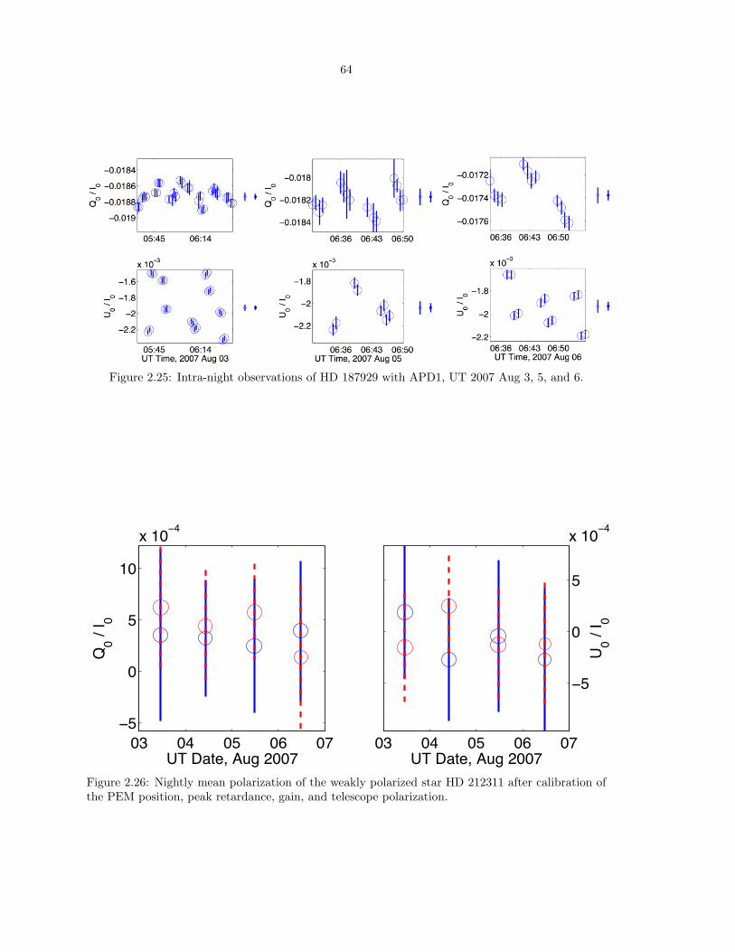
64

Figure 2.25: Intra-night observations of HD 187929 with APD1, UT 2007 Aug 3, 5, and 6.

03 04 05 06 07−5

0

5

10

x 10−4

UT Date, Aug 2007

Q0 /

I 0

03 04 05 06 07

−5

0

5

x 10−4

UT Date, Aug 2007

U 0 / I 0


Figure 2.26: Nightly mean polarization of the weakly polarized star HD 212311 after calibration ofthe PEM position, peak retardance, gain, and telescope polarization.

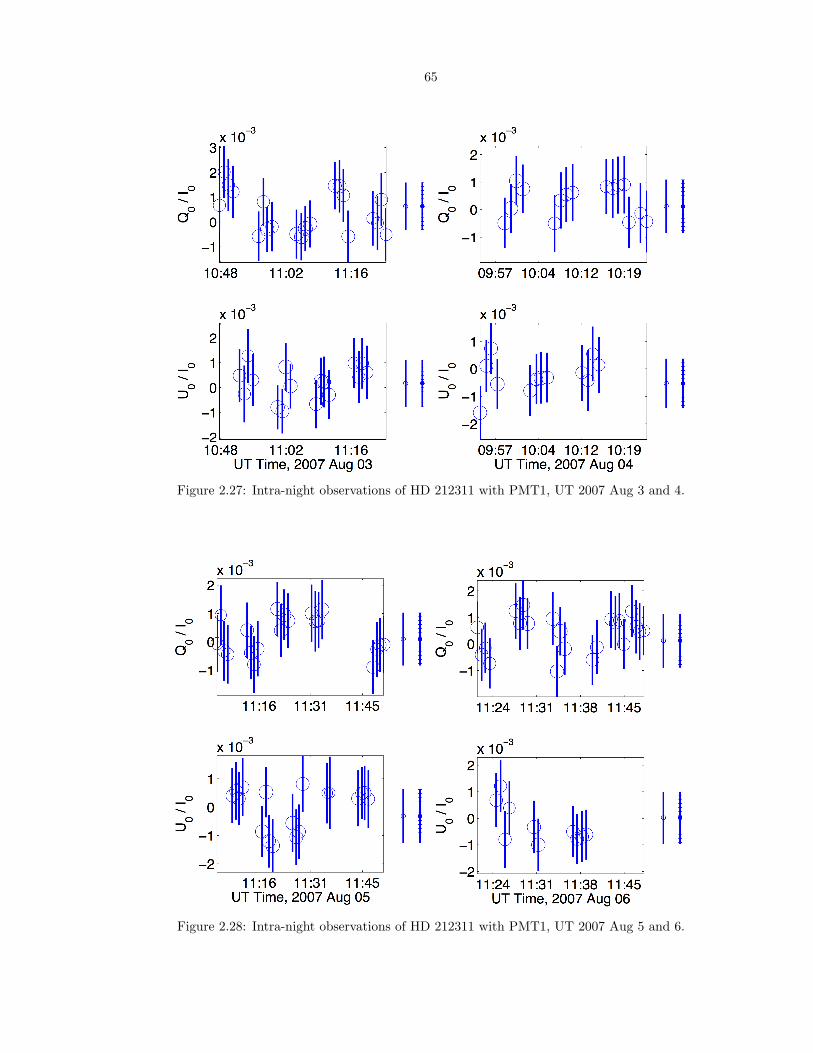
65

Figure 2.27: Intra-night observations of HD 212311 with PMT1, UT 2007 Aug 3 and 4.

Figure 2.28: Intra-night observations of HD 212311 with PMT1, UT 2007 Aug 5 and 6.

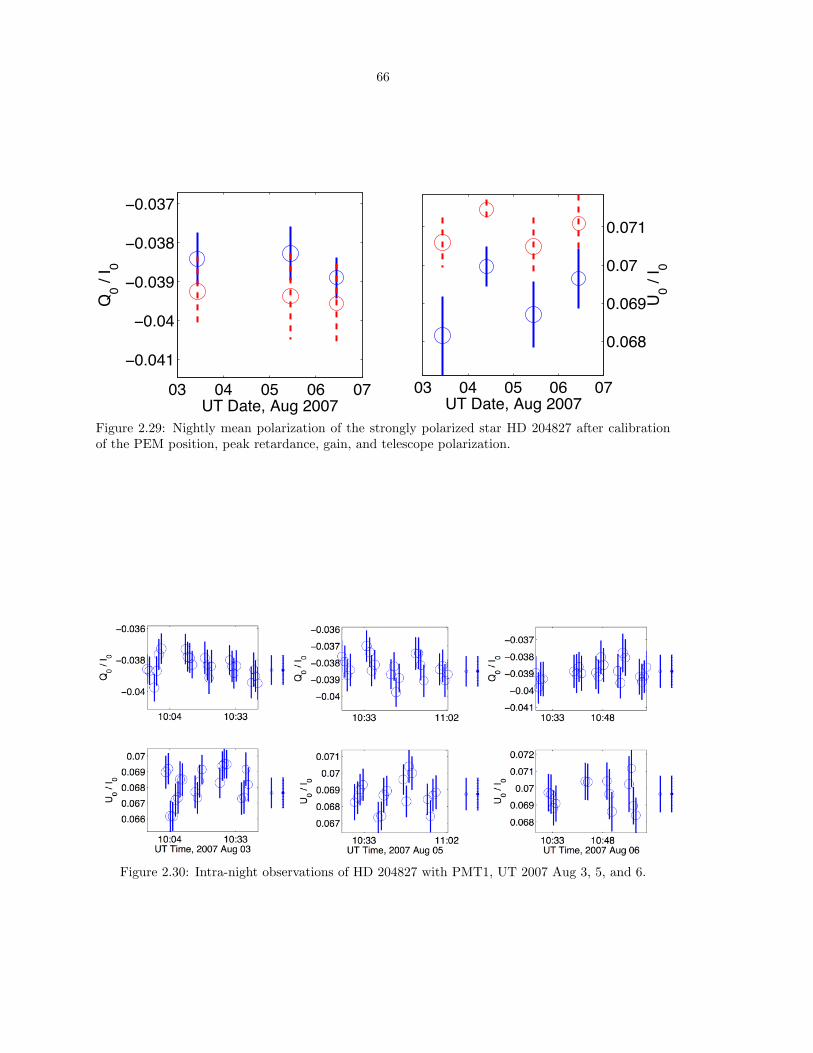
66

03 04 05 06 07

−0.041

−0.04

−0.039

−0.038

−0.037

UT Date, Aug 2007

Q0 /

I 0

03 04 05 06 07

0.068

0.069

0.07

0.071

UT Date, Aug 2007

U 0 / I 0



Figure 2.30: Intra-night observations of HD 204827 with PMT1, UT 2007 Aug 3, 5, and 6.

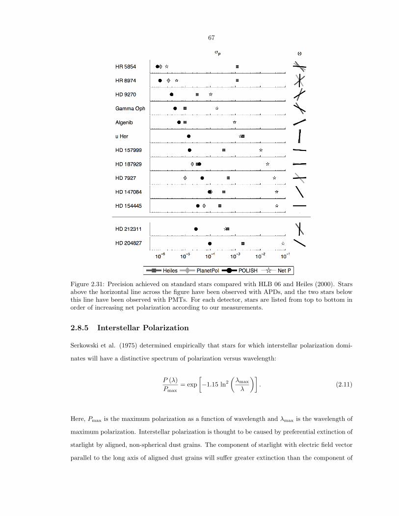
67

Figure 2.31: Precision achieved on standard stars compared with HLB 06 and Heiles (2000). Starsabove the horizontal line across the figure have been observed with APDs, and the two stars belowthis line have been observed with PMTs. For each detector, stars are listed from top to bottom inorder of increasing net polarization according to our measurements.

2.8.5 Interstellar Polarization

Serkowski et al. (1975) determined empirically that stars for which interstellar polarization domi-

nates will have a distinctive spectrum of polarization versus wavelength:

P (λ)Pmax

= exp[−1.15 ln2

(λmax

λ

)]. (2.11)

Here, Pmax is the maximum polarization as a function of wavelength and λmax is the wavelength of

maximum polarization. Interstellar polarization is thought to be caused by preferential extinction of

starlight by aligned, non-spherical dust grains. The component of starlight with electric field vector

parallel to the long axis of aligned dust grains will suffer greater extinction than the component of

68

the electric field perpendicular to the long axis of the grains (Davis & Greenstein 1951). The exact

cause of grain alignment is debated, but presence of magnetic fields is a significant component.

Of the stars observed in Table 2.2, the following have been investigated by Serkowski et al.

(1975): HD 7927, HD 147084, HD 154445, HD 157999, HD 187929, and HD 204827. All of these

have wavelength dependence of polarization indicative of interstellar polarization, which implies that

intrinsic polarization does not dominate for these stars. Indeed, Schmidt et al. (1992) find good fits

of their data to interstellar polarization curves for HD 7927, HD 154445, and HD 204827.

2.9 Discussion

We have commissioned a high precision, integrated light polarimeter in order to detect variability in

the optical, linear polarization of high mass X-ray binaries. This variability should be indicative of

system inclination, and high precision monitoring is hoped to constrain the black hole mass in these

systems. While results from observations of Cygnus X-1 will be in Chapter 4, we report on the high

precision attained on standard stars.

Noise on individual measurements of most stars is comparable to photon shot noise (Figures 2.11

to 2.30). When combining measurements, we obtained precision on most stars that is comparable

to PlanetPol, a similar instrument mounted on the William Herschel Telescope (HLB 06). Precision

achieved on unpolarized stars is up to three orders of magnitude better than listed in the combined

polarimetric catalogs of Heiles (2000), and precision on strongly polarized stars is improved by up to

an order of magnitude. The large improvement in polarimetric precision arises from the combination

of large telescope aperture, a high-quality polarization modulator, and high frequency modulation.

We find night-to-night precision of three to ten parts per million on bright, weakly polarized

standard stars(10−4 < P < 10−3

). This precision increases as σP ∝ P

12 , where it reaches about

one part in 104 for stars with P between one and ten percent. Thus, night-to-night precision scales

as expected from photon shot noise statistics. Consultation of Tables 2.10 and 2.13 shows that

systematic effects reveal themselves at the level of ≈ 1% of the measured polarization. The night-

to-night noise floor of the instrument appears to be eight parts in ten million even in the presence of

telescope polarization on the order of one part in 104. High precision monitoring of stellar variability

is discussed in the next chapter.

69

References

Aspin, C., Simmons, J. F. L, & Brown, J. C. 1981, MNRAS 194, 283.

Bastien, P., Drissen, L., Menard, F., Moffat, A. F. J., Robert, C. & St-Louis, N. 1988, AJ 95, 900.

Brown, J. C., Ignace, R., & Cassinelli, J. P. 2000, A&A 356, 619.

Davis, L., Jr. & Greenstein, J. L. 1951, ApJ 114, 206.

Dolan, J. F. & Tapia, S. 1989, ApJ 344, 830.

Friend, D. B. & Cassinelli, J. P. 1986, ApJ 303, 292.

Gies, D. R., and 10 coauthors. 2003, ApJ 583, 424.

Hamamatsu Photonics K.K. 1999, “Photomultiplier Tubes: Basics and Applications”, 2nd Ed.

Heiles, C. 2000, AJ 119, 923.

Hough, J. H., Lucas, P. W., Bailey, J. A., Tamura, M., Hirst, E., Harrison, D., & Bartholomew-Biggs,

M. 2006, PASP 118, 1302.

Hsu, J.-C. & Breger, M. 1982, ApJ 262, 732.

Kemp, J. C. 1969, J. Opt. Soc. Am. 59, 950.

Kemp, J. C., Barbour, M. S., Parker, T. E., & Herman, L. C. 1979, ApJ 228, L23.

McClintock, J. E., Shafee, R., Narayan, R., Remillard, R. A., Davis, S. W., & Li, L.-X. 2006, ApJ

652, 518.

Milgrom, M. 1979, A&A 76, 338.

Oke, J. B. 1961, ApJ 133, 90.

Schmidt, G. D., Elston, R., & Lupie, O. 1992, AJ 104, 1563.

Serkowski, K., Mathewson, D. S., & Ford, V. L. 1975, ApJ 196, 261.

Wolinski, K. G., Dolan, J. F., Boyd, P. T., Biggs, J. D., Nelson, M. J., Percival, J. W., Taylor, M.,

& van Citters, G. W. 1996, ApJ 457, 859.

Ziolkowski, J. 2005, MNRAS 358, 851.

70

2.10 Appendix A: Mueller Matrix for Lab Tests

Mueller matrices describe how the polarization state of incident light is modified by optical compo-

nents. For the lab tests in section 2.5.2, the polarizing components employed are a linear polarizer

and Wollaston prism, so the Mueller matrix of the system is

M = MW × T−ψ ×Mpol × Tψ (A1)

Starting from the left hand side of Equation A1, the matrices represent the Wollaston, the rotation

matrix for the linear polarizer at angle ψ with respect to the Wollaston axis, and the Mueller matrix

for the polarizer. Incident light is first affected by the Mueller matrix at the end of the equation,

and the incident polarization state is successively modified by the matrices to the left. That is,

Iobs

Qobs

Uobs

Vobs

= M

I0

Q0

U0

V0

(A2)

where I0, Q0, U0, and V0 are the Stokes parameters of the incident light and Iobs, Qobs, Uobs, and

Vobs are the observed Stokes parameters. For this system,

Iobs

Qobs

Uobs

Vobs

=T

2

1 ±1 0 0

±1 1 0 0

0 0 0 0

0 0 0 0

×

1 0 0 0

0 cos 2ψ − sin 2ψ 0

0 sin 2ψ cos 2ψ 0

0 0 0 1

×

1 1 0 0

1 1 0 0

0 0 0 0

0 0 0 0

×

1 0 0 0

0 cos 2ψ sin 2ψ 0

0 − sin 2ψ cos 2ψ 0

0 0 0 1

×

I0

Q0

U0

V0

(A3)

where T = 25±2% is the transmission of the polarizer. A perfect polarizer is assumed, which passes

no light with polarization perpendicular to its axis. The PEM was disabled for this test, and only

71

the DC reading from the voltmeters was used. Thus, the average intensity is

Iobs =T

2[I0 (1 + cos 2ψ) +Q0 cos 2ψ (1 + cos 2ψ) + U0 sin 2ψ (1 + cos 2ψ)] (A4)

The LED is essentially unpolarized, so Q0 ≈ U0 ≈ 0 and Equation A4 reduces to

I ≈ TI0 (1 + cos 2ψ) (A5)

2.11 Appendix B: Mueller Matrix for POLISH

In general, the Mueller matrix of POLISH is given by

MPOLISH = T−φ ×MD ×ML ×MW ×MB × T−θPEM ×MPEM × TθPEM × Tφ ×MT (B1)

Starting from the left hand side of Equation B1, the matrices are the rotation matrix for Cassegrain

ring angle φ, the Mueller matrices for the detector window, field lenses, Wollaston prism, and beam-

splitter, the rotation matrix for PEM angle θ ≡ θPEM, the Mueller matrix for the PEM, and the

Mueller matrix for the telescope. Subtraction of telescope polarization is necessary to calibrate for

MT.

Since the PEM and Wollaston prism convert the polarization of the incident light into intensity

modulation, the polarization state of light past the Wollaston is not our concern. The reflection

of light off the beamsplitter is at nearly 90◦ and is stable during observations, so any polarization

imparted to the light by the beamsplitter is just a constant offset to the polarization. Therefore,

we only consider the throughput of the detector window, field lenses, and beamsplitter. We denote

the throughput of the instrument as E, and it is given in section 2.3. The POLISH Mueller matrix

becomes

72

MPOLISH = E

0BBBBBBB@

1 0 0 0

0 cos 2φ − sin 2φ 0

0 sin 2φ cos 2φ 0

0 0 0 1

1CCCCCCCA×

0BBBBBBB@

0.5 ±0.5 0 0

±0.5 0.5 0 0

0 0 0 0

0 0 0 0

1CCCCCCCA×

0BBBBBBB@

1 0 0 0

0 cos 2θ − sin 2θ 0

0 sin 2θ cos 2θ 0

0 0 0 1

1CCCCCCCA

×

0BBBBBBB@

1 0 0 0

0 1 0 0

0 0 cosβ sinβ

0 0 − sinβ cosβ

1CCCCCCCA×

0BBBBBBB@

1 0 0 0

0 cos 2θ sin 2θ 0

0 − sin 2θ cos 2θ 0

0 0 0 1

1CCCCCCCA×

0BBBBBBB@

1 0 0 0

0 cos 2φ sin 2φ 0

0 − sin 2φ cos 2φ 0

0 0 0 1

1CCCCCCCA(B2)

The instantaneous retardance of the PEM is given by β = α + β0 sinωt. The retardance offset of

the PEM, α, is assumed to be negligible from calibration by Hinds Instruments, Inc. Note that

ω = 2π × 50.12 kHz. The top sign in the Wollaston matrix (+) indicates the left beam which

reaches detector 2, and the bottom sign (−) represents the right beam which reaches detector 1.

The instrumental Mueller matrix, listed by columns one through four, now becomes

MPOLISH (:, 1) = E/2

0BBBBBBB@

1

± cos 2φ

± sin 2φ

0

1CCCCCCCA(B3a)


0BBBBBBB@

±ˆ`

cos2 2θ + sin2 2θ cosβ´

cos 2φ− 1/2 sin 4θ (1− cosβ) sin 2φ˜

`cos2 2θ + sin2 2θ cosβ

´cos2 2φ− 1/4 sin 4θ (1− cosβ) sin 4φ

1/2ˆ`


sin 4φ− sin 4θ (1− cosβ) sin2 2φ˜

0

1CCCCCCCA(B3b)


0BBBBBBB@

±ˆ`


sin 2φ+ 1/2 sin 4θ (1− cosβ) cos 2φ˜

1/2ˆ`


sin 4φ+ sin 4θ (1− cosβ) cos2 2φ˜

`cos2 2θ + sin2 2θ cosβ

´sin2 2φ+ 1/4 sin 4θ (1− cosβ) sin 4φ

0

1CCCCCCCA(B3c)


0BBBBBBB@

∓ sin 2θ sinβ

− sin 2θ sinβ cos 2φ

− sin 2θ sinβ sin 2φ

0

1CCCCCCCA(B3d)

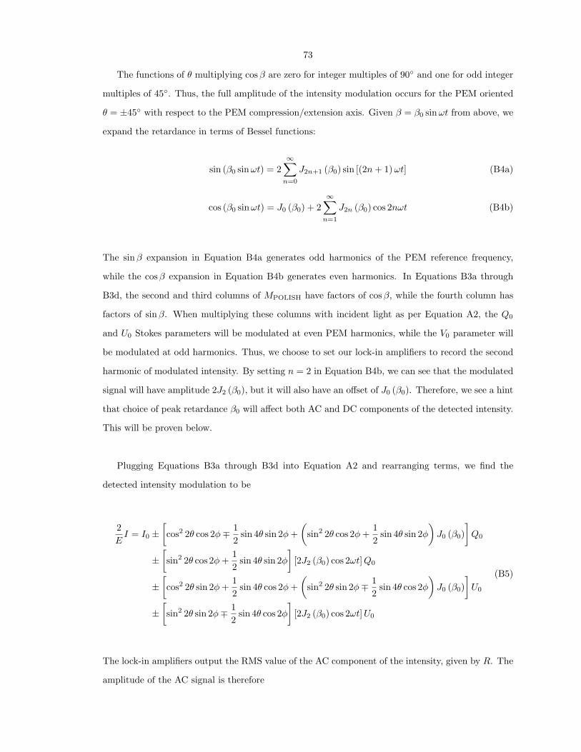
73

The functions of θ multiplying cosβ are zero for integer multiples of 90◦ and one for odd integer

multiples of 45◦. Thus, the full amplitude of the intensity modulation occurs for the PEM oriented

θ = ±45◦ with respect to the PEM compression/extension axis. Given β = β0 sinωt from above, we

expand the retardance in terms of Bessel functions:

sin (β0 sinωt) = 2∞∑n=0

J2n+1 (β0) sin [(2n+ 1)ωt] (B4a)

cos (β0 sinωt) = J0 (β0) + 2∞∑n=1

J2n (β0) cos 2nωt (B4b)

The sinβ expansion in Equation B4a generates odd harmonics of the PEM reference frequency,

while the cosβ expansion in Equation B4b generates even harmonics. In Equations B3a through

B3d, the second and third columns of MPOLISH have factors of cosβ, while the fourth column has

factors of sinβ. When multiplying these columns with incident light as per Equation A2, the Q0

and U0 Stokes parameters will be modulated at even PEM harmonics, while the V0 parameter will

be modulated at odd harmonics. Thus, we choose to set our lock-in amplifiers to record the second

harmonic of modulated intensity. By setting n = 2 in Equation B4b, we can see that the modulated

signal will have amplitude 2J2 (β0), but it will also have an offset of J0 (β0). Therefore, we see a hint

that choice of peak retardance β0 will affect both AC and DC components of the detected intensity.

This will be proven below.

Plugging Equations B3a through B3d into Equation A2 and rearranging terms, we find the

detected intensity modulation to be

2EI = I0 ±

[cos2 2θ cos 2φ∓ 1

2sin 4θ sin 2φ+

(sin2 2θ cos 2φ+

12

sin 4θ sin 2φ)J0 (β0)

]Q0

±[sin2 2θ cos 2φ+

12

sin 4θ sin 2φ]

[2J2 (β0) cos 2ωt]Q0

±[cos2 2θ sin 2φ+

12

sin 4θ cos 2φ+(

sin2 2θ sin 2φ∓ 12

sin 4θ cos 2φ)J0 (β0)

]U0

±[sin2 2θ sin 2φ∓ 1

2sin 4θ cos 2φ

][2J2 (β0) cos 2ωt]U0

(B5)

The lock-in amplifiers output the RMS value of the AC component of the intensity, given by R. The

amplitude of the AC signal is therefore

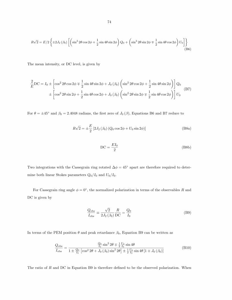
74

R√

2 = E/2

±2J2 (β0)

»„sin2 2θ cos 2φ+

1

2sin 4θ sin 2φ

«Q0 +

„sin2 2θ sin 2φ∓ 1

2sin 4θ cos 2φ

«U0

–ff(B6)

The mean intensity, or DC level, is given by

2E

DC = I0 ±[cos2 2θ cos 2φ∓ 1

2sin 4θ sin 2φ+ J0 (β0)

(sin2 2θ cos 2φ+

12

sin 4θ sin 2φ)]

Q0

±[cos2 2θ sin 2φ+

12

sin 4θ cos 2φ+ J0 (β0)(

sin2 2θ sin 2φ∓ 12

sin 4θ cos 2φ)]

U0

(B7)

For θ = ±45◦ and β0 = 2.4048 radians, the first zero of J0 (β), Equations B6 and B7 reduce to

R√

2 = ±E2

[2J2 (β0) (Q0 cos 2φ+ U0 sin 2φ)] (B8a)

DC =EI0

2(B8b)

Two integrations with the Cassegrain ring rotated ∆φ = 45◦ apart are therefore required to deter-

mine both linear Stokes parameters Q0/I0 and U0/I0.

For Cassegrain ring angle φ = 0◦, the normalized polarization in terms of the observables R and

DC is given by

Qobs

Iobs≡

√2

2J2 (β0)R

DC=Q0

I0(B9)

In terms of the PEM position θ and peak retardance β0, Equation B9 can be written as

Qobs

Iobs=

Q0I0

sin2 2θ ∓ 12U0I0

sin 4θ

1± Q0I0

[cos2 2θ + J0 (β0) sin2 2θ

]± 1

2U0I0

sin 4θ [1∓ J0 (β0)](B10)

The ratio of R and DC in Equation B9 is therefore defined to be the observed polarization. When

75

defining the PEM efficiency as EPEM = 2J2 (β0), and noting the definition of R from Equation 2.3a,

Equation B9 reduces to Equation 2.4. The PEM efficiency is the strength of the intensity modu-

lation for a given polarization. Maximum efficiency of EPEM = 97.1% is achieved for retardance

of π radians (halfwave retardance), while our choice of β0 = 2.4048 radians results in EPEM = 86.4%.

For θ 6= ±45◦ and/or β0 6= 2.4048 radians, the observed polarization Qobs/Uobs can still be used

to determine the true polarization Q0/U0. In general,

Q0

I0=

QobsIobs

{1± 1

2U0I0

sin 4θ [1∓ J0 (β0)]}± 1

2U0I0

sin 4θ

sin2 2θ ∓ QobsIobs

[cos2 2θ + J0 (β0) sin2 2θ

] (B11a)

U0

I0=

UobsIobs

{1± 1

2Q0I0

sin 4θ [∓1 + J0 (β0)]}− 1

2Q0I0

sin 4θ

sin2 2θ ∓ UobsIobs

[cos2 2θ + J0 (β0) sin2 2θ

] (B11b)

The decreased efficiency by using β0 = 2.4048 instead of π radians decreases the AC signal from

polarized stars by a factor of J2 (π) /J2 (2.4048) = 1.12, and it will slightly decrease the signal to noise

ratio of polarimetric measurements using POLISH. However, the choice of β0 = π radians coupled

with PEM misalignment (θ 6= ±45◦) magnifies the amount of U0/I0 that leaks into measurements

of Qobs/Iobs, and vice versa, by a factor of

1− J0 (π)1− J0 (2.4048)

= 1.30 (B12)

We therefore use a peak retardance of β0 = 2.4048 radians in our measurements.

2.12 Appendix C: Detector Noise

Given pre-gain signal current i0 and pre-gain dark current id, the number of pre-gain photoelectrons

during an integration of duration tAC, and the shot noise on this quantity, will be given by

n =(i0 + id) tAC

e(C1a)

σn =[

(i0 + id) tAC

e

] 12

(C1b)

76

The pre-gain shot noise current is essentially the pre-gain shot noise in electrons times e/tAC, because

current has units of coulombs per second. This value is

σi =[

2eB (i0 + id)tAC

] 12

(C2)

where B is the system bandwidth in Hz and will be discussed later. The factor of√

2 comes about

when converting between photocurrent and photoelectrons. The post-gain shot noise current is

σ′i = G

[2eBF (i0 + id)

tAC

] 12

(C3)

where G is detector gain and

F ≈ Gx (C4)

is the gain noise factor (post-gain quantities are primed). This factor arises because the gain process

itself has statistical fluctuations. The excess noise factor, x, is a constant. Thus, we find the

post-gain shot noise current to be

σ′i =[

2eBG2+x (i0 + id)tAC

] 12

(C5)

Since voltage is measured at the output of the detectors, we convert signal and dark current to

signal and dark voltage. The pre-gain signal and dark current are therefore

i0 =DCGTA

(C6a)

id =i′dG

(C6b)

where TA is the amplifier transimpedance in V/A and the post-gain dark current is i′d. Output noise

voltage is related to noise current by σ′v = TAσ′i, so we plug Equations C6a and C6b into Equation

C5 and multiply by the transimpedance to find

77

σ′v =[

2eBG1+xTA(DC + i′dTA)tAC

] 12

(C7)

This is the expected voltage noise on the output of the detectors. We now relate this quantity to

fluctuations in the observables X, Y , and DC.

In general, error propagation on a function g(x1, x2, · · · , xj) is given by

σg =

∑j

(∂g

∂xjσxj

)2 1

2

(C8)

By propagating error through Equation 2.4, we find polarimetric uncertainty of a measurement to

be related to uncertainty in X, Y , and DC according to

σP =√

22J2 (β0) DC

(X2σ2

X + Y 2σ2Y

X2 + Y 2+X2 + Y 2

DC2 σ2DC

) 12

(C9)

Rearranging terms, and absorbing the t−1/2AC factor from Equation C7, we find

σP =√

2EPEMDC

{1tAC

[X2σ2

X + Y 2σ2Y

X2 + Y 2+

12

(EPEMPσDC)2

]} 12

(C10)

For an imperfect detector, expected voltage noise is given by Equation C7. However, we must

determine the bandwidth B with care. Photon shot noise is white noise, which means that it occurs

at all frequencies. However, it clearly cannot continue up to infinite frequency, because integrated

power would also be infinite. The maximum frequency at which photon shot noise can occur will

be the count rate of noise photons. Thus, we determine maximum bandwidth by the square root of

the number of detected photons,

Bmax =(

DCeGTA

) 12

(C11)

The detectors have bandwidth ranging from about 100 kHz to 200 kHz. However, the lock-in am-

78

plifiers only admit noise in a bandwidth of BAC ≈ 2.6 Hz, while the voltmeters have bandwidth of

BDC ≈ 1 MHz. Thus, the bandwidth for shot noise on X and Y will be min(Bmax, Bdetector, BAC) =

BAC for all stars. The bandwidth for shot noise on DC will be min(Bmax, Bdetector, BDC), which will

depend on stellar intensity.

Using Equation C7, we can determine photon shot noise (x = 0 and i′d = 0) and detector noise

(x 6= 0 and i′d 6= 0) on X, Y , and DC. We can also compare these values to the observed fluctuations

during each measurement.

σX

σY

σDC

shot

= γ0

BAC

BAC

min (Bmax, Bdetector)

12

(C12a)

σX

σY

σDC

detector

= γ

BAC

BAC

min (Bmax, Bdetector)

12

(C12b)

σX

σY

σDC

obs

=

std(Xsrc)2 + std(Xsky)2

std(Ysrc)2 + std(Ysky)2

std(DCsrc)2 + std(DCsky)2

12

(C12c)

Here, γ0 ≡ 2eGTADC, γ ≡ 2eG1+xTA(DC + i′dTA), and “std” indicates the sample standard devia-

tion. Finally, inserting Equations C12a through C12c into Equation C10 yields the uncertainty in

polarization from photon shot noise, detector noise, and observed fluctuations.

For the APDs, the gain noise factor is quoted as F = 2.2 at gain G = 300. From Equation C4,

we find xAPD = 0.138. For the PMTs, the gain noise factor is as follows (Hamamatsu Photonics

1999):

F =1ε

(1 +

K∑k=1

1δk

)(C13)

where ε is the PMT collection efficiency, δk is the secondary electron emission ratio at each dynode

k, and K is the number of dynodes (the multiplicative regions of the PMT). The PMT collection

79

efficiency ε is the fraction of photoelectrons emitted by the photocathode that reach the first dynode.

Assuming ε = 1 and δk = δ (all dynodes have the same gain),

F =δ

δ − 1(C14)

and gain is simply G = δK . Since the PMT gain over its nine dynodes is 5 × 106 from Table 2.3,

δ = 0.55, F = 1.2, and x = 0.013. That is, gain from the PMTs is an order of magnitude less noisy

than from the APDs, which is why PMTs are preferred over APDs for faint objects.

the polish instrument - caltechthesisthesis.library.caltech.edu/857/3/02chapter2.pdfthe polish...

Documents