the pattern of visual deficits in amblyopia - center for neural science

Journal of Vision (2003) 3, 380-405 http://journalofvision.org/3/5/5/ 380

The pattern of visual deficits in amblyopia

Suzanne P. McKee Smith-Kettlewell Institute of Visual Sciences,

San Francisco, CA, USA

Dennis M. Levi School of Optometry, University of California,

Berkeley, CA, USA

J. Anthony Movshon Center for Neural Science, New York University,

New York, NY, USA

Amblyopia is usually defined as a deficit in optotype (Snellen) acuity with no detectable organic cause. We asked whether this visual abnormality is completely characterized by the deficit in optotype acuity, or whether it has distinct forms that are determined by the conditions associated with the acuity loss, such as strabismus or anisometropia. To decide this issue, we measured optotype acuity, Vernier acuity, grating acuity, contrast sensitivity, and binocular function in 427 adults with amblyopia or with risk factors for amblyopia and in a comparison group of 68 normal observers. Optotype acuity accounts for much of the variance in Vernier and grating acuity, and somewhat less of the variance in contrast sensitivity. Nevertheless, there are differences in the patterns of visual loss among the clinically defined categories, particularly between strabismic and anisometropic categories. We used factor analysis to create a succinct representation of our measurement space. This analysis revealed two main dimensions of variation in the visual performance of our abnormal sample, one related to the visual acuity measures (optotype, Vernier, and grating acuity) and the other related to the contrast sensitivity measures (Pelli-Robson and edge contrast sensitivity). Representing our data in this space reveals distinctive distributions of visual loss for different patient categories, and suggests that two consequences of the associated conditions – reduced resolution and loss of binocularity – determine the pattern of visual deficit. Non-binocular observers with mild-to-moderate acuity deficits have, on average, better monocular contrast sensitivity than do binocular observers with the same acuity loss. Despite their superior contrast sensitivity, non-binocular observers typically have poorer optotype acuity and Vernier acuity, at a given level of grating acuity, than those with residual binocular function.

Keywords: amblyopia, spatial vision, contrast sensitivity, Vernier acuity, binocular vision

1. Introduction Amblyopia, a developmental disorder that degrades

spatial vision and stereopsis, is almost always associated with strabismus, anisometropia, or form deprivation early in life. In adults, amblyopia is usually diagnosed by a significant reduction in optotype (Snellen) visual acuity, which cannot be improved by refractive correction and which has no obvious organic cause. It has become customary to identify patients as strabismic or anisometrope amblyopes if those conditions are evident when the patients are studied. Strabismus and anisometropia can cause amblyopia, but they can also both arise as a consequence of amblyopia (Lepard, 1975; Kiorpes & Wallman, 1995; Birch & Swanson, 2000). So the relationship between strabismus, anisometropia, and amblyopia is complex, and the conditions associated with amblyopia in adulthood may not be the ones that were important in creating amblyopia. It is therefore desirable to know whether the visual performance of different amblyopes shows a distinctive pattern of variation that might reflect different causal factors, independently of the associated condition. Amblyopia might be multifactorial, but it could also be a simpler abnormality that varies in severity but not in kind. In this case, amblyopia could be

completely characterized by a single measure, such as optotype acuity, regardless of the associated clinical condition. Optotype acuity would predict the losses in other visual functions, independent of the patient’s clinical status.

For many years, it has been proposed that there are differences in visual functioning between strabismic and anisometropic amblyopes, beyond the obvious differences associated with oculomotor behavior (Von Noorden, l967; Shapero, l971; Duke-Elder, l973). Most psychophysical studies have used measures of contrast sensitivity and acuity to explore these presumed differences. These studies on small numbers of amblyopes have reached diverse conclusions about whether anisometropic and strabismic amblyopes have different patterns of visual loss (Levi & Klein, 1985; Bradley & Freeman, 1985b; Hess & Holliday, 1992; Birch & Swanson, 2000). For example, Levi, Klein, and their colleagues compared grating acuity, Vernier acuity, and optotype acuity in strabismic and anisometropic amblyopes (Levi and Klein 1982a, 1982b, l985; Levi, Klein & Yap, l987; Levi, Klein & Wang, l994a, 1994b). They found that in amblyopes with strabismus, the deficits in optotype acuity and in Vernier acuity were disproportionately greater than the deficit in grating

DOI 10:1167/3.5.5 Received November 11, 2002; published July 15, 2003 ISSN 1534-7362 © 2003 ARVO

McKee, Levi, & Movshon 381

acuity, whereas in amblyopes with anisometropia, the deficits in optotype and Vernier acuity were nearly proportional to the deficit in grating acuity (Levi & Klein 1982a, 1982b, l985). In a recent study based on 53 amblyopes, Birch and Swanson (2000) showed that, among moderate amblyopes, the ratio of Vernier to grating acuity was significantly different between anisometropes and strabismics, following the pattern of the Levi and Klein studies. However, among the severe amblyopes in their study, this difference between anisometropes and strabismics was not evident. Birch and Swanson suggested that functional distinctions between different clinical groups might depend on the range of severity of the deficit in the population studied.

Thus, despite numerous studies, it remains unclear whether there are distinctive patterns of visual loss in strabismic and anisometropic amblyopes, much less in other clinically defined categories. The limited repertoire of psychophysical measurements may account for this uncertainty, but the reasons for choosing acuity and contrast measures to investigate this issue are entirely defensible. Amblyopia is a developmental abnormality of visual cortex (Hubel & Wiesel, l965; Wiesel & Hubel, l963; Eggers & Blakemore, l978; Harrad, Sengpiel, & Blakemore, l996; Horton & Hocking, l996; Kiorpes, Kiper, O’Keefe, Cavanaugh, & Movshon, 1998; Kiorpes & Movshon, 2003). Contrast sensitivity and acuity are thought to be limited by early visual processing (Lennie, 1998), so these measurements should reveal whatever differences exist among amblyopic subgroups. We suggest that it is the small number of subjects, rather than the choice of psychophysical measurements, that accounts for the inability to find consistent functional patterns. Broadly speaking, the deficits seen in amblyopic individuals are similar, no matter what the presenting condition, so, in small samples, individual variation may obscure subtle distinctions among subgroups. To discern functional patterns, if they exist, we need a much larger sample of human observers.

We recruited a large sample of adult abnormal observers (427), including individuals who were currently amblyopic, and those who had been at risk for amblyopia during development because of associated conditions such as strabismus, as well as a control group of 68 normal observers. In addition to optotype acuity, we measured four other visual functions that are known to be abnormal in amblyopia: contrast sensitivity, grating acuity, Vernier acuity, and binocularity. Our results show that measuring optotype acuity captures much of the variance in the other functional measurements. Nevertheless, we readily identified significant differences in the patterns of visual loss among the clinically defined categories, particularly between strabismic and anisometropic observers. An important determinant of the pattern of functional visual loss is whether the abnormal observer has residual binocular function in the central visual field. In addition to the measurements described in this paper, we made other

sensory and oculomotor measurements, some of which were described in Schor, Fusaro, Wilson, and McKee (l997); reports of our other findings are in preparation. We have briefly reported some of these results elsewhere (Movshon, McKee, & Levi, 1996; McKee, l998; Movshon, McKee, & Levi, 2003).

2. Methods

2.1 Psychophysical Methods 2.1.1 Stimuli

The stimuli for all of the psychophysical measures were presented on a Princeton Max-15 monitor with a screen size of 19.7 x 25.5 cm, a frame rate of 60 Hz, and, unless otherwise specified, a mean luminance of 90 cd/m2.

2.1.2 Grating Acuity We measured grating acuity with high-contrast (80%)

horizontal sinusoidal gratings, usually viewed at 6 m. The viewing distance was 3 m for amblyopes with Snellen acuities between 20/200 and 20/600, and was reduced to 1 m for amblyopes with acuity worse than 20/600, so that a sufficient number of cycles were present at the limit of acuity.

The grating was vignetted by an elliptical two-dimensional Gaussian that subtended ≈ 1.7 deg x 1.2 deg at 6 m, and was proportionally larger at closer viewing distances. Grating contrast was ramped on over 200 msec,

and after a 500 msec plateau, was ramped off over 200 msec. The starting spatial frequency was set at roughly two thirds of the cut-off frequency estimated from the LogMAR acuity. In subsequent trials, spatial frequency was varied by a staircase procedure that increased spatial frequency following three correct responses and decreased spatial frequency after one incorrect response. Approximately one third of the trials were blanks. The staircase was terminated after six reversals. The acuity threshold was taken as the geometric mean of the last four reversals. No feedback was provided.

2.1.3 Vernier Acuity The stimulus consisted of five high-contrast (95%)

offset pairs of horizontal lines, each ≈ 0.14' wide and 43' long when viewed at the normal distance of 6 m. At this distance, the entire pattern subtended 1.43 x 1.1 deg; the vertical interline separation was 14.3'; the members of each pair were separated horizontally by ≈ 0.14'. To obtain subpixel offsets, the luminance profile of the lines was dithered. For observers with grating acuities lower than 30 c/deg, the viewing distance in meters was set to one fifth of the cutoff frequency to insure visibility. The stimuli were ramped on over 200 msec, and after a 500-msec plateau, were ramped off over 200 msec.


Each test began with an adjustment procedure in which the operator increased the offset until the patient reported that the right side was higher or lower than the left side. The mean offset obtained from four adjustments (two up and two down) was used as the starting step size for a forced-choice blocked staircase method. Each block consisted of 20 trials randomly chosen with one of four possible offsets (1 or 2 steps up; 1 or 2 steps down). The observer's task was to indicate whether the offset was up or down on each trial by pressing one of two response buttons. In the initial block, the step size was determined from the preceding method of adjustment procedure. In subsequent blocks, the step size was increased or decreased depending on the observer's performance in the preceding 20-trial block. The maximum step size was set equal to one fourth the interline distance; the minimum step size was 2.3" (at 6 m). No feedback was given. We estimated Vernier threshold as half the difference between the 25% and 75% points on a psychometric function compiled from all four blocks (80 forced-choice responses), using probit analysis.

2.1.7 Binocular Motion Integration We used the dichoptic quadrature motion stimulus

devised by Shadlen and Carney (1986) to evaluate binocular motion integration (BMI). Each eye viewed a horizontal sinusoidal grating whose contrast modulated sinusoidally at 2 Hz. Stimuli in the two eyes were spatially and temporally 90 deg out of phase with each other; the direction of the phase shifts determines whether the binocularly summed signal appears to move up or down. Observers viewed the two gratings on adjacent halves of the monitor divided by a septum. The perceived contrast of the two eyes' gratings was matched prior to the test to equate the strength of the signals in the two eyes: the contrast of a 0.38 c/deg grating seen in the lower visual field of the right eye was set to match the contrast of a 0.38 c/deg grating seen in the upper visual field of the left eye. Grating contrast was roughly 5 times the threshold contrast for edge detection. To insure appropriate alignment, the observer adjusted Risley biprisms in front of each eye until a fixation pattern superimposed on the gratings was fused and the four horizontal nonius lines in each eye's image were aligned. Once the nonius lines were aligned, the observer was given 30 “motion” trials in which they were shown the matched dichoptic stimuli for 2 s, and judged the direction of movement. Feedback was provided after each trial. If the observer was correct on 20 or fewer of the 30 trials, we halted the test and assigned a score of 0. Otherwise the contrast matching procedure was repeated in turn for 0.75, 1.5, 3.0, and 6.0 c/deg gratings, and we presented 20 motion trials at each of these four spatial frequencies. We estimated the maximum spatial frequency for binocular motion integration as the 75% point on a Weibull function fitted to the percentage correct data. If the observer’s performance was at or near chance for these four spatial frequencies, we assigned a score of 0.38.

2.1.4 Edge Contrast Sensitivity Contrast detection thresholds were measured for a

horizontal edge (luminance step) that was vignetted by an elliptical two-dimensional Gaussian. The vignette subtended ≈ 0.86 x 0.62 deg at the normal viewing distance of 6 m, and was ramped on- and off over 200 msec, with a 500-msec plateau. The mean luminance was 74 cd/m2. Viewing distance was scaled by grating acuity as for Vernier acuity. We used a yes-no staircase procedure without feedback, similar to the one used for the grating acuity test. The staircase (ending after six reversals) decreased the edge contrast by 20% following three correct responses, and increased edge contrast after one incorrect response. The initial contrast was 0.0575. One third of the trials were blanks. Threshold was taken as the geometric mean of the last four reversals. 2.1.8 Stereo-Optical Circles Test

We also measured stereopsis using the Randot “Circles” test (Stereo Optical Co, Chicago, IL), a test recommended by Simons (1981) for use with this kind of patient population. This test was administered according to the instructions supplied by the manufacturer. The patient was shown the test at a distance of 40.6 cm.

2.1.5 Pelli-Robson Contrast Sensitivity We also measured contrast sensitivity with a Pelli-

Robson contrast sensitivity chart, viewed at 1 m. The Pelli-Robson chart utilizes letters of the same size but with decreasing contrast; in each row the letters decrease in contrast in proportional steps from left to right, and also from top to bottom. The observer is required to identify the letters. Performance was evaluated using the standardized method recommended by the test designers (Pelli, Robson, & Wilkins, l988).

2.1.9 Test-Retest Reliability We estimated the reliability of our measures by retesting 23 observers, drawn from all categories. The Pearson and Spearman rank correlations for each of the psychophysical measures are given in Table 1. The scores indicate reasonably good test-retest reliability for Snellen acuity, Vernier acuity, and grating acuity, and poorer reliability for the two measures of contrast sensitivity.

2.1.6 Optotype (Snellen) Acuity Optotype acuity was measured with a modified Bailey-

Lovie (LogMAR) chart, as used in the Early Treatment Diabetic Retinopathy Study (ETDRS, l985). Observers viewed the chart with their best visual correction at a distance of 3 m at a background luminance of 61 cd/m2. The test was scored on a letter-by-letter basis.


Table 1. Test-Retest Reliability

Measure Pearson Spearman

Grating acuity 0.89 0.93

Vernier acuity 0.82 0.90

Edge contrast threshold 0.24 0.18

Pelli-Robson contrast threshold 0.45 0.67

Snellen acuity 0.98 0.98

• High refractive error – refractive error exceeding 4 D spherical equivalent in either eye.

• Noncentric fixation – monocular fixation in either eye more than 0.5 deg from the center of the fovea, as determined by visuoscope.

• Deprivation – a history of visual deprivation, e.g., by cataract, ptosis, etc.

• Normal – none of the above. Pearson and Spearman correlation coefficients for 23 subjects from the abnormal groups. 2.2.1 Patient Categories

The attributes associated with each category are as follows: 2.2 Observers Normals (n = 68) Four hundred and ninety-five observers, between the

ages of 8 and 40, participated in this study. Each adult signed a consent form that described the purpose of the study and the visual testing procedures; a parent or guardian of each minor signed the consent form. Of the 548 people who underwent clinical examination, we excluded 43 because of ocular pathology, bilaterally reduced vision, or poor responsiveness; 10 withdrew before completing the psychophysical testing.

• Normal

Anisometropes (n = 84)

• Unequal refractive error • No constant or inconstant ocular deviation • No noncentric fixation • No deprivation • No surgical history

Each observer was given a complete clinical examination, performed by one of 6 study clinicians (3 ophthalmologists and 3 optometrists, who all underwent training in the standardized clinical protocol). Information about ocular history was obtained from medical records, if available, and/or conversations with the patient or the patient’s parent. Refractive error was measured under both cycloplegic and noncycloplegic conditions. Visual acuity was evaluated by the Bailey-Lovie LogMAR test measured with best optical correction. Horizontal and vertical angles of deviation were quantified with a prism-cover test at 0.3 m and 6 m.

During unilateral and alternating cover tests, each eye was covered for at least 5 s. Eccentric fixation was determined with a visuoscope on each eye separately, while the other eye was occluded.

Strabismic-anisometropes (n = 101) • Constant ocular deviation • No deprivation • Unequal refractive error

Strabismics (n = 40) • Constant ocular deviation • No deprivation • No unequal refractive error

Former Strabismics (n = 18) • Surgical history • No constant or inconstant ocular deviation • No deprivation

Eccentric fixators (n = 35) It is important to appreciate that we distinguished the

attributes measured in the clinical examination from the categories to which we assigned each patient. The patient attributes used for classification were:

• Noncentric monocular fixation • No constant or inconstant ocular deviation • No deprivation • No surgical history

• Constant ocular deviation – failure of binocular eye alignment under all testing conditions. Cover-testing was performed at both “distance” (6 m) and “near” (0.3 m).

Deprivationals (n = 24) • History of deprivation (history of ptosis, cataract, or

ocular ulceration)

Refractives (n = 27) • Inconstant deviation – a failure of binocular eye alignment that is not consistent under all testing conditions, i.e., the deviation is not always present.

• High refractive error • No unequal refractive error • No constant or inconstant ocular deviation • Surgical history – a history of surgery to correct a defect

of eye alignment. • No deprivation • No noncentric fixation • Unequal refractive error – a difference in refractive error

between the eyes of at least 1 D at the worst meridian. • No surgical history


Other abnormals (n = 30) • No noncentric fixation (or centricity of fixation could

be determined) • No surgical history • Another anomaly, such as • History of patching • History of anisometropia • Oculomotor abnormalities other than strabismic, e.g.,

jerk nystagmus

Note that many of these categories are different from those traditionally used for classifying amblyopia. (For clarity, throughout this work, we use italics for the names of the categories.) For example, the strabismic category does not include everyone with an ocular deviation. A strabismic is defined here as an observer currently exhibiting a constant horizontal and/or a vertical deviation at both 0.3 and 6 m, and having a difference in refractive error of less than 1 D and no history of deprivational conditions (e.g., cataract or ptosis). So while all strabismics are strabismic, not all strabismics are strabismic. An anisometrope is defined as a patient with a difference in refractive error between the eyes of 1 D or more at the most anisometropic meridian (based on the manifest dry refraction), a fixation eccentricity of less than 0.5 deg, and no evidence of either horizontal or vertical deviation at either distance. If the clinician was unable to determine fixation eccentricity, the patient was not included in the anisometropic group, but was relegated to the other abnormal category.

The prevalence of amblyopia depends on the optotype acuity criterion used to define the minimum deficit (Flom & Neumaier, l966). For purposes of this study, we used a conservative criterion (20/40) that has been used in many previous studies. We should point out that the acuity of our normal observers was 20/17 on average, and was never worse than 20/30 in either eye, so an optotype acuity worse than 20/30 may have been a more reasonable choice for defining amblyopia. For the most part, our analyses do not distinguish amblyopic from nonamblyopic observers, so the particular criterion used is largely inconsequential.

This research followed the tenets of the World Medical Association Declaration of Helsinki, and was approved by the appropriate Institutional Review Boards.

2.3 Statistical Analyses Parametric tests of statistical inference are commonly

used to assess the likelihood that an observed difference between groups could have arisen by chance – the “null” hypothesis. These tests usually rely on the assumption that the data are normally distributed. As our data violated this assumption, standard statistical measures were not appropriate. We considered various nonparametric methods, but rejected them because they lack power and are often difficult to tailor to precise

analytic questions. Instead, we used a numerical technique, permutation analysis, to estimate the sampling distribution of the differences that could arise by chance partitioning of a data set, a distribution instantiating the null hypothesis (Efron & Tibshirani, l993). Such techniques can be used to answer statistical questions exactly and without bias, while making no strong assumptions about the nature and distribution of the data. For most of our comparisons, we first combined all members of two designated test groups into a single pool, and then randomly assigned the members to two groups of the same size as the original test groups. We then took suitable measures of the difference between these two randomly assigned groups, stored the values, and repeated the whole process 1,000-2,000 times. The resulting distribution of differences is the one that could have arisen by chance combination between samples of the same size as the original test samples, drawn from the same population. If the observed difference between the original test groups lay outside the body of the distribution generated by random assignment, then we assert that the probability that the observed difference could have been generated by chance was less than 0.0005 (1/2000). If the observed difference lay within the range of differences generated by random assignment, we estimated how frequently a difference this large or larger would occur by chance, So, for example, if 4/2000 (0.002) of the permuted differences were as large or larger than the observed difference, we assigned an exact probability of 0.002. All our reports of the significance of the differences between groups are based on such permutation computations.

Wherever possible, we present the raw data (Figures 2-6, Figure 11, and Figure 13). To create a succinct representation of this vast array of data and to reduce the number of potential comparisons (five measurements across 11 categories), we also performed a factor analysis, using PCA, on normalized distributions of our measurements. As shown by the raw data, the distributions of our measurements were typically skewed and highly non-normal, so we transformed the raw log data so that they approximated normality, using a variation of Tukey’s “ladder of transformations” (Tukey, 1977). We first offset each measurement set so that the median for all observers equaled 1, and then applied a compressive nonlinear transform using the Michaelis-Menten equation

′ x =xn

x n + σ n (1) with σ and n chosen separately for each set of measurements so that the cumulative data were approximately linear when plotted as Z scores (i.e., so that they fit the form of a cumulative normal distribution). The resulting transformed-to-normal data conformed acceptably to a five-dimensional Gaussian, and formed the basis for the factor analysis.


Factor analysis is used here as a “descriptive” statistic; again all statistical inferences about differences between groups are based on permutations of their factor scores. The PCA analysis was done with the aid of the SPSS software package (SPSS Inc.; http://www.spss.com).

3. Results

3.1 Variation and Covariation of Acuity and Sensitivity Across the Population

Based on a 20/40 acuity criterion, roughly half (219/427, 51%) of the abnormal observers in our sample were amblyopic. Figure 1 summarizes the distribution of LogMAR acuity measurements across our population; optotype acuity is plotted in LogMAR units (top axis) and in min arc (bottom axis) for easy graphical comparison to our other acuity measures. Recall that a LogMAR acuity of 0.3 is the same as a threshold of 2 min and a Snellen acuity of 20/40. The solid shading indicates the cases in each category in which acuity fell below the 20/40 criterion. The colors of the shaded areas are based on a broad categorization of amblyopes that we will develop later in this paper; here it can be interpreted to indicate functional affinities among categories of the same color. The right column shows data for the non-preferred eye for each clinical category. The left column shows – using an expanded scale – the distribution of acuities of the preferred eyes for each category. It is interesting that the preferred eyes of normal observers have, on average, slightly better acuity than the preferred eyes of abnormal observers in all categories – an advantage that is highly significant statistically (see also Kandel, Grattan, & Bedell, l980).

Amblyopia was most prevalent among the strabismic-anisometropes (81%) and least prevalent (4%) among the refractive group. The variations from category to category in the percentage of amblyopic observers must be interpreted with caution. Since our objective was to measure visual functions in a large number of amblyopes, our study population was enriched in individuals with functional visual deficits and was in no sense a random sample of the population of observers with particular clinical conditions. Previous studies have found different distributions of patient conditions in their samples of amblyopes (Flom & Neumaier, 1966; Flynn & Cassady, l978). In the sample assembled from all the amblyopes (90) participating in studies in several laboratories, Ciuffreda, Levi, and Selenow (1991) found roughly equal numbers of strabismic, anisometropic, and strabismic-anisometropic observers. They did, however, find a disproportionate number of strabismic-anisometropic observers among amblyopes with severe visual loss (>20/100), a finding similar to that shown in Figure 1. Thus, the relatively high proportion of amblyopes in our

strabismic-anisometropic group may be related to the high percentage (46%) of amblyopes with acuities worse than 20/100 in our total sample.

Figure 2 plots four scatter diagrams showing the relationships between optotype acuity and grating acuity, Vernier acuity, Pelli-Robson contrast threshold, and edge contrast threshold for the non-preferred eyes of our whole population of 495 observers. Data from normal observers are shown with crosses, while colored points show data from abnormal observers. The colors chosen are the same as in Figure 1, and represent three functional groups of amblyopes that will be distinguished later in this paper. The solid lines are not conventional regression lines but are best-fitting straight lines that take account of the variance of the two dependent measures being plotted (Press, Teukolsky, Vetterling, & Flannery, 1992). The lines in each panel are fitted only to the data in color, from the 427 abnormal observers. Each panel is labeled with the slope of the best-fitting line and with the Pearson correlation between the plotted variables. Because all the data are plotted on logarithmic scales, the slopes of the lines correspond to the exponents of power functions that capture the main relationships between pairs of variables. It is evident from Figure 2 that these functions provide an acceptable description of the main trends in the data.

The two upper panels of Figure 2 show that both grating acuity and Vernier acuity have a strong correlation with optotype acuity. Confirming earlier studies (Levi & Klein, 1982a, 1982b), the loss in Vernier acuity is almost directly proportional to the loss in optotype acuity; the exponent of the power function indicated by the best-fitting line in the top panel is 1.15. As has also been shown by previous studies (Gstalder & Green, l971; Mayer, Fulton, & Rodier, l984), the loss in grating acuity is on average smaller than the corresponding loss in optotype acuity; the exponent of the best-fitting power function is 0.65, but the correlation value is high. This result means that for an “average” amblyope with acuity of 20/80, (about 4 times worse than normal), Vernier acuity would be 4.9 times worse than normal, but grating acuity would be only 2.5 times worse than normal.

The two lower panels of Figure 2 show that our two measures of contrast sensitivity have a much weaker relationship to optotype acuity. The Pelli-Robson contrast threshold (third panel) shows a moderate increase (exponent = 0.30) with increasing amblyopia. The correlation between Pelli-Robson threshold and LogMAR acuity is moderately strong, but accounts for less than 40% of the variance in the two measures. The edge contrast threshold (bottom panel) shows a very modest increase with optotype acuity (exponent = 0.18), and also a rather low correlation that accounts for less than 10% of the variance in the two measures. Even the most severe amblyopes in our sample are only about 3 times worse in contrast sensitivity than average normal observers. Indeed, the range of edge contrast thresholds for the normals nearly equals the abnormal range. These measures

http://www.spss.com/


Figure 1. Distrieye and on the20/40 = LogMAexplained belo

-0.5 0.0 0.5 1.0 1.5 2.0 2.5

0.0

0.2

0.4Normalsn=68, 0% amblyopes

0.0

0.2Anisometropesn=84, 43% amblyopes

0.0

0.2Strabismic anisometropesn=101, 81% amblyopes

0.0

0.2Strabismicsn=40, 48% amblyopes

0.0

0.2

Inconstant strabismicanisometropesn=44, 39% amblyopes

0.0

0.2Inconstant strabismicsn=24, 29% amblyopes

0.0

0.2Former strabismicsn=18, 34% amblyopes

0.0

0.2Eccentric fixatorsn=35, 69% amblyopes

0.0

0.2Deprivationalsn=24, 42% amblyopes

0.0

0.2Refractivesn=27, 4% amblyopes

0.0

0.2Other abnormalsn=30, 40% amblyopes

1 3 10 30 100 300

-0.5 0.0 0.5

LogMAR acuity

0.0

0.2

0.0

0.2

0.0

0.2

0.0

0.2

0.0

0.2

0.0

0.2

0.0

0.2

0.0

0.2

0.0

0.2

0.0

0.2

0.0

0.2

0.4 1 2

Pro

port

ion

of c

ases

Optotype acuity (min)

Preferred eyes Non-preferred eyes

butions of optotype acuity in each of our clinically defined categories. The distributions on the left are for the preferred right are for the non-preferred eye. The colored columns show the amblyopes (defined as Snellen acuity worse than R of 0.3 = 2 min arc) in each category. The colors indicate a postulated grouping of clinical categories that will be w.


indicate that the deficit in contrast sensitivity near the peak of the contrast sensitivity function (CSF) is minimal in most human amblyopes (see also Hess, Campbell, & Zimmern, l980; Selby & Woodehouse, l981; Bradley & Freeman, l985a, 1985b; Harrad & Hess, l992).

1 3 10 30 100

0.1

0.3

1

3

10

30

Ver

nier

acu

ity (

min

)

slope=1.15r=0.88

1 3 10 30 100

1

3

10

30

100

Gra

ting

acui

ty (

min

)

slope=0.65r=0.80

1 3 10 30 100

0.01

0.03

0.1

Pel

li-R

obso

nco

ntra

st th

resh

old

slope=0.30r=0.61

1 3 10 30 100Optotype acuity (min)

0.01

0.03

0.1

Edg

eco

ntra

st th

resh

old

slope=0.18r=0.29

3.2 Distributions of Visual Function Across Patient Categories

Are the functional relationships shown in Figure 2 the same for all patient categories? We approach this question by examining these relationships separately for different categories of observers. To simplify this comparison, we pooled the inconstant strabismics (24), the inconstant strabismic-anisometropes (44), and the former strabismics (18) into a single large group, which we call sporadic strabismics. We set aside the data for the refractives, because most refractives have normal or nearly normal acuity in both eyes, and also the data from the other abnormals because this group is so heterogeneous. The results from the remaining five abnormal categories and the sporadic strabismics are plotted in separate graphs in Figures 3-6.

Each of these figures uses a standard format – the individual data from each of the six patient categories are plotted in a panel that includes the best-fitting straight line copied from Figure 2. Because these lines were fit to the data for all abnormal observers, the relationship between the data for a particular patient group and the plotted line provides a visual indication of whether that patient group’s data deviate from the overall trend.

Figure 2. Because these lines were fit to the data for all abnormal observers, the relationship between the data for a particular patient group and the plotted line provides a visual indication of whether that patient group’s data deviate from the overall trend.

To test such deviations statistically, we used a permutation analysis (see “Methods”). We randomly sampled sets of data from the whole abnormal population of the size corresponding to the patient group size (e.g., 84 cases for the anisometropes). We fit lines to each of the randomly chosen subsamples, and then established the probability that the slope and intercept for the line fitted to the patient group’s data fell outside the distribution of slopes and intercepts obtained by chance permutation. We repeated this procedure for each of the groups and comparisons in Figures 3-6, 24 in all. We took deviations to be significant when the associated probability was lower than 0.0021 (corresponding to a value of 0.05 with a full Bonferroni correction for 24 independent tests). Large asterisks in each figure indicate cases that showed significant deviations by this rather strict criterion.

To test such deviations statistically, we used a permutation analysis (see “Methods”). We randomly sampled sets of data from the whole abnormal population of the size corresponding to the patient group size (e.g., 84 cases for the anisometropes). We fit lines to each of the randomly chosen subsamples, and then established the probability that the slope and intercept for the line fitted to the patient group’s data fell outside the distribution of slopes and intercepts obtained by chance permutation. We repeated this procedure for each of the groups and comparisons in Figures 3-6, 24 in all. We took deviations to be significant when the associated probability was lower than 0.0021 (corresponding to a value of 0.05 with a full Bonferroni correction for 24 independent tests). Large asterisks in each figure indicate cases that showed significant deviations by this rather strict criterion.

Figure 2. Four psychophysical measures are plotted against optotype acuity for the non-preferred eye for the entire sample. The crosses show the normal observers. The solid lines are the lines fitted to the data from the abnormal observers (colored symbols), according to the procedure in Press et al. (l992, section 15.3), which takes account of the variance in the two dependent measures that are being related. Two outliers (one deprivational and one deep anisometrope, ~15D) gave wildly deviant Pelli-Robson values and have been omitted from that plot.


Figure 3. Six grapsolid lines are thethe category wascomposite of threobservers in the

1 3 10 30 100

0.1

0.3

1

3

10

30

Anisometropes (84)

1 3 10 30 100

0.1

0.3

1

3

10

30

Ver

nier

acu

ity (

min

)

Strabismic anisometropes (101)

1 3 10 30 100

0.1

0.3

1

3

10

30

Strabismics (40)

Sporadic strabismics (86)1 3 10 30 100

0.1

0.3

1

3

10

30

Eccentric fixators (35)1 3 10 30 100

0.1

0.3

1

3

10

30

Deprivationals (24)1 3 10 30 100


0.1

0.3

1

3

10

30

hs plotting Vernier threshold against optotype acuity for the non-preferred eye for each of six clinical categories. The ones that were fitted to the whole abnormal population and are taken from Figure 2. The large asterisks indicate that significantly different from the whole sample, either in slope or intercept (see text). The sporadic strabismics are a e categories: inconstant strabismic-anisometropes, inconstant strabismics and former strabismics. Data from refractive, other abnormal, and normal categories are not shown.

∗

∗


Figure 3 plots Vernier acuity against optotype acuity for the six abnormal groups. The major qualitative difference among the graphs is the difference in the range, rather than in the pattern of loss. In particular, the scatterplot for the acuities of strabismic-anisometropes spans roughly 2 log units on both axes, while the acuities for the strabismics and anisometropes span only about 1 log unit.

Permutation analysis revealed that the data for two groups, anisometropes and strabismics, deviated significantly from the overall trend, which can also be seen by inspecting the relation between the data points for each

group and the plotted line. Recall from Figure 2 that the exponent for all abnormals was 1.15, meaning that the relationship between Vernier and optotype acuity was nearly proportional. For the anisometropes, this exponent was 1.44, while for the strabismics it was 0.79. In fair agreement with these values, Levi and Klein (1982b) found that the Vernier-optotype acuity exponent for their 10 anisometropes was 1.1 + 0.15, while the exponent for their 14 strabismics was 0.8 + 0.04. Generally, Vernier acuity in anisometropes is somewhat worse than expected from their optotype acuity, while Vernier acuity in

Figure 4. Scatte

1 3 10 30 100

1

3

10

30

100

1 3 10 30 100

1

3

10

30

100

Gra

ting

acui

ty (

min

)

1 3 10 30 100

1

3

10

30

100

1 3 10 30 100

1

3

10

30

100

1 3 10 30 100

1

3

10

30

100


1

3

10

30

100

Anisometropes (84)


Strabismics (40)

Sporadic strabismics (86)

Eccentric fixators (35)

Deprivationals (24)

∗

∗

rplots, in the same format as Figure 3, showing grating acuity against optotype acuity for the non-preferred eye.


strabismics is somewhat better. Figure 4 plots grating acuity against optotype acuity

for the six abnormal groups. For all groups, the loss in grating acuity is less than the corresponding loss in optotype acuity (the exponent for all abnormals in Figure 2 was 0.65). Permutation analysis again revealed two groups whose data deviate from the overall trend. The strabismic group has a visibly shallower slope than the whole abnormal population; the exponent for this group is 0.31. The strabismic anisometrope group differs from the whole abnormal population not in exponent but in the intercept of the fitted line – on average, the grating acuity of members of this group was roughly 15% lower than for the whole abnormal population, for any given level of optotype acuity. This is evident from the prevalence of points in the plot that fall below the line. These results partially confirm the findings of Levi and Klein (1982a, 1982b, 1985), by showing that the relationship between grating and optotype acuity in amblyopes with strabismus is different from the relationship in other amblyopes.

Figure 5 plots Pelli-Robson contrast threshold against optotype acuity for the six abnormal groups. All groups

show a relationship with the same low exponent, close to the abnormal average from Figure 2 of 0.30. Permutation analysis again reveals two groups, strabismic anisometropes and strabismics, which differ significantly from the whole abnormal population. In both cases, the main difference is in the mean value of the contrast threshold – for a given value of optotype acuity, these observers, on average, had contrast thresholds that were 16% lower (i.e., better) than for the abnormal group as a whole. This effect leads to the prevalence of data points in the relevant panels that fall below the fitted line. It is noteworthy that these two groups are the same groups that showed significant deviations in the comparison of grating acuity with optotype acuity (Figure 4). These groups thus have grating acuity and contrast sensitivity that are slightly better than the whole abnormal population, when variations in optotype acuity are factored out.

Figure 6 plots edge contrast threshold against optotype acuity for the six abnormal groups. As with the Pelli-Robson threshold data from Figure 5, all groups show a similar shallow slope, close to the average

Figure 5. Scattnon-preferred

1 3 10 30 100

0.01

0.03

0.1

1 3 10 30 100

0.01

0.03

0.1

Pel

li-R

obso

n co

ntra

st th

resh

old

1 3 10 30 100


0.01

0.03

0.1

1 3 10 30 100

0.01

0.03

0.1

1 3 10 30 100

0.01

0.03

0.1

1 3 10 30 100

0.01

0.03

0.1

Anisometropes (84)

Strabismicanisometropes (101)

Strabismics (40)



Deprivationals (24)

erplots, in the same format as Figure 3, showing Pelli-Robson contrast threshold against optotype acuity for the eye.

∗

∗


exponent of 0.18 for all abnormals. Permutation analysis reveals two groups that deviate significantly, anisometropes and strabismic anisometropes. As in the case of Pelli-Robson contrast thresholds, these groups differ from the whole abnormal population not by the slope of the relationship but by the mean of the thresholds. Anisometropes, for a given level of optotype acuity, have edge contrast thresholds that are 28% higher (i.e., worse) than the whole population, while strabismic anisometropes have edge contrast thresholds that are 26% lower (i.e., better) than the whole population. This can be seen by the prevalence of data points above and below the fitted line in the two relevant panels.

We draw two conclusions from the data shown in these 24 graphs. First, amblyopia is not a single abnormality that is completely characterized by optotype acuity. If all amblyopes (and individuals at risk for amblyopia) were identical save for random variation, then all the data in these figures would be scattered around the fitted lines, and none of the permutation tests would have yielded a significant deviation at the strict criterion level we used. Instead, 8 of the 24 comparisons revealed

significant deviations. Second, these deviations suggest that there are systematic differences among strabismics, strabismic anisometropes, and anisometropes, because these are the categories involved in the eight cases with significant deviations from the whole abnormal sample.

3.3 Factor Analysis of Category Characteristics

To make comparisons among categories more tractable, we performed a factor analysis of our five measurements to determine how many explanatory variables were needed to characterize the underlying functional losses. The analysis produced evidence for two explanatory factors, which we transformed using Oblimin rotation so that they were roughly orthogonal. These factors represent linear combinations of the five tranformed measurements; the relationship between the measurements and the factors is shown by the vectors in Figure 7. One factor loads heavily on the acuity measures (optotype, Vernier, and grating), and the other loads on the contrast sensitivity measures (edge contrast and Pelli-

1 3

∗

∗10 30 100

0.01

0.03

0.1

1 3 10 30 100

0.01

0.03

0.1

Edg

e co

ntra

st th

resh

old


0.01

0.03

0.1

1 3 10 30 100

0.01

0.03

0.1

1 3 10 30 100

0.01

0.03

0.1

1 3 10 30 100

0.01

0.03

0.1

Anisometropes (84)

Strabismicanisometropes (101)

Strabismics (40)



Deprivationals (24)

Figure 6. Scatterplots, in the same format as Figure 3, showing edge contrast threshold against optotype acuity for the non-preferred eye.


Robson contrast thresholds). This outcome can be understood by noting the inter-measurement correlations described above – the three acuity measures were highly correlated with each other, and the contrast threshold measures were also correlated with each other. Factor 1, the “acuity” factor, accounts for 52% of the variance in the data set. Factor 2, the “sensitivity” factor, accounts for a further 29%. Together these two factors account for more than 80% of the variance. We ran many variants of the factor analysis, but no variant produced evidence for a significant third factor – such a factor, when included, typically accounted for less than 9% of the variance.

Next, we transformed the data from our subjects into factor scores using the loadings shown in Figure 7, and replotted them in this new coordinate system. In this space, differences among the clinical categories are more readily apparent. Figure 8 shows the results for four major sub-groups: normals, anisometropes, strabismics, and strabismic-anisometropes, plotted on a background showing all the abnormal data. The normals lie to the right of the other three groups, meaning that their acuity factor is superior to the others. For each of the three abnormal groups in Figure 8, the data fall in an elliptical cloud along a diagonal slice of this space. The slope of the ellipses indicates that, as amblyopia becomes more severe, sensitivity and acuity decline together. However, the strabismic data occupy a different slice from the anisometropic data, lying generally to the left and above. In other words, for each value of the acuity factor, the strabismics, on average, show a higher sensitivity than the

anisometropes. Indeed, a number of strabismics show sensitivity values that are superior to the values of the normals.

The strabismic-anisometropic observers appear to have factor scores that deviate from the normals roughly as would be expected from a combination of the deviations of the strabismic and anisometropic groups. For moderate acuity loss, they resemble the strabismics, showing the same supernormal sensitivity on average, whereas for severe acuity loss, their sensitivity declines to that of the anisometropic observers. Nevertheless, a close inspection of the strabismic-anisometropic distribution reveals that the centroid of this group is shifted leftward along the acuity axis. Even the strabismic-anisometropes with supernormal contrast sensitivity show diminished acuity relative to the strabismics, presumably because of the presence of anisometropia. This pattern suggests that, among strabismic anisometropes, strabismus dominates visual functions in mild-to-moderate amblyopes, but that anisometropia dominates visual loss in severe amblyopes.

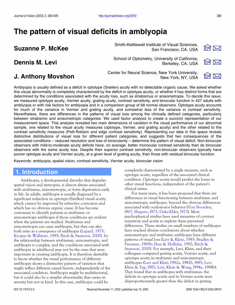
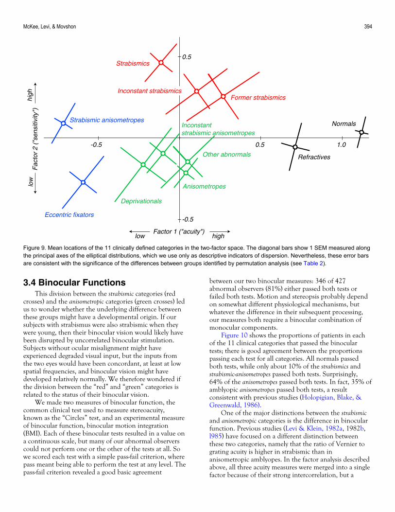
Figure 9 plots the mean factor values for all 11 clinical categories. The oblique bars SEs estimated along the major and minor principal axes of these elliptical distributions (cf. Figure 8). The principal axis of variation for each group runs obliquely up and to the right, meaning that within each group, individuals with better acuity tend also to have better sensitivity. Note that the scales in this graph are expanded relative to Figure 9, so that the differences among the categories are easier to see. To a first approximation, the overlap of the error bars represents the significance of the differences among these groups, but we computed more precise estimates of

0.0 0.5Loading on factor 1

0.0

0.5

Load

ing

on fa

ctor

2

Grating acuity

Edge contrast sensitivity

Vernieacuity

Log MAR acuity

Pelli-Robson contrast sensitivity

Figure 7. The relationship between each of our five measurements for the two factors (explanatory variables) identified by factor analysis. Factor 1 is closely related to all three acuity measures, and Factor 2 is closely related to the two contrast sensitivity measures.

significance with a permutation analysis. Table 2 lists the significance of all possible intergroup comparisons in the factor space of Figure 9. Comparing Figure 9 and Table 2 shows the rationale behind the coloring of the four super-groups in Figure 9. Within each color key, group differences tend not to be significant; between color keys, almost all group differences are significant. The coloring in Figure 9 therefore captures our view that there are four broad categories of observers in our sample: normal or near-normal (black), moderate acuity loss with superior (red) or impaired (green) sensitivity, and severe acuity loss (blue). It may now be helpful to refer back to Figures 1 and 2, which use this color scheme to identify members of these three groups. It is difficult to discern the patterns revealed in Figures 8 and 9 by inspection of the raw data in Figures 1 and 2. The location of these groups in the two-factor space is reasonable if one considers the nature of the accompanying conditions. Deprivationals and anisometropes share conditions that blur or degrade image quality, so they should lie adjacent to one another. Many eccentric fixators are probably strabismic-anisometropes with such a severe visual acuity loss that the weak eye does not move when the preferred eye is covered, because no shift in visual direction is detected. Therefore, this group should lie in the same place as severely amblyopic


strabismic-anisometropes. The separation between the strabismic and anisometropic categories, apparent in Figure 8, is even more evident in Figure 9. All the “pure” strabismic categories (i.e., without anisometropia) show

supernormal sensitivity, well above that of the anisometropes. Yet, despite their poor sensitivity, the anisometropes show an acuity that is as good or perhaps lightly better than the strabismics. s

Figure 8.anisomea mixture

Factor 1 ("acuity")highlow

Fac

tor

2 ("

sens

itivi

ty")

high

low

-3

3

2-3

Strabismicanisometropes

(101)

-3

3

2-3

Strabismics (40)

-3

3

2-3

Anisometropes(84)

-3

3

2-3

Normals (68)

Scatterplots showing the factor-variable scores for observers in four of the clinical categories. The normal, strabismic and tropic observers fall into different regions of the two-factor space. The strabismic-anisometropic observers appear to represent of the strabismic and anisometropic categories.


-0.5 0.5 1.0

-0.5

0.5

Normals

Anisometropes

Deprivationals

Eccentric fixators

Inconstantstrabismic anisometropes

Other abnormals Refractives

Strabismic anisometropes


Fac

tor

2 ("

sens

itivi

ty")

high

low

Figure 9. Mean locations of the 11 clinically defined categories in the two-factor space. The diagonal bars show 1 SEM measured along the principal axes of the elliptical distributions, which we use only as descriptive indicators of dispersion. Nevertheless, these error bars are consistent with the significance of the differences between groups identified by permutation analysis (see Table 2).

Former strabismics

Strabismics

Inconstant strabismics

3.4 Binocular Functions This division between the strabismic categories (red

crosses) and the anisometropic categories (green crosses) led us to wonder whether the underlying difference between these groups might have a developmental origin. If our subjects with strabismus were also strabismic when they were young, then their binocular vision would likely have been disrupted by uncorrelated binocular stimulation. Subjects without ocular misalignment might have experienced degraded visual input, but the inputs from the two eyes would have been concordant, at least at low spatial frequencies, and binocular vision might have developed relatively normally. We therefore wondered if the division between the “red” and “green” categories is related to the status of their binocular vision.

We made two measures of binocular function, the common clinical test used to measure stereoacuity, known as the “Circles” test, and an experimental measure of binocular function, binocular motion integration (BMI). Each of these binocular tests resulted in a value on a continuous scale, but many of our abnormal observers could not perform one or the other of the tests at all. So we scored each test with a simple pass-fail criterion, where pass meant being able to perform the test at any level. The pass-fail criterion revealed a good basic agreement

between our two binocular measures: 346 of 427 abnormal observers (81%) either passed both tests or failed both tests. Motion and stereopsis probably depend on somewhat different physiological mechanisms, but whatever the difference in their subsequent processing, our measures both require a binocular combination of monocular components.

Figure 10 shows the proportions of patients in each of the 11 clinical categories that passed the binocular tests; there is good agreement between the proportions passing each test for all categories. All normals passed both tests, while only about 10% of the strabismics and strabismic-anisometropes passed both tests. Surprisingly, 64% of the anisometropes passed both tests. In fact, 35% of amblyopic anisometropes passed both tests, a result consistent with previous studies (Holopigian, Blake, & Greenwald, 1986).

One of the major distinctions between the strabismic and anisometropic categories is the difference in binocular function. Previous studies (Levi & Klein, 1982a, 1982b, l985) have focused on a different distinction between these two categories, namely that the ratio of Vernier to grating acuity is higher in strabismic than in anisometropic amblyopes. In the factor analysis described above, all three acuity measures were merged into a single factor because of their strong intercorrelation, but a


Table 2. Probabilities of Obtaining Observed Intergroup Differences by Chance

Nor

mal

s

Ani

som

etro

pes

Str

abis

mic

s

Str

abis

mic

an

isom

etro

pes

Inco

nsta

nt s

trab

ism

ics

Inco

nsta

nt s

trab

ism

ic

anis

omet

rope

s

For

mer

str

abis

mic

s

Ecc

entr

ic fi

xato

rs

Dep

rivat

iona

ls

Ref

ract

ives

Anisometropes 0.0000

Strabismics 0.0000 0.0000

Strabismic- anisometropes 0.0000 0.0000 0.0060

Inconstant strabismics 0.0000 0.0030 0.2500 0.0010

Inconstant strabismic- anisometropes 0.0000 0.1595 0.0290 0.0015 0.1605

Former strabismics 0.0010 0.0070 0.1300 0.0045 0.9065 0.1905

Eccentric fixators 0.0000 0.0210 0.0020 0.1955 0.0105 0.0330 0.0070

Deprivationals 0.0000 0.8685 0.0280 0.0230 0.0810 0.6170 0.1335 0.2505

Refractives 0.0175 0.0000 0.0000 0.0000 0.0030 0.0015 0.0365 0.0000 0.0065

Other abnormals 0.0000 0.0945 0.0570 0.0005 0.4415 0.7515 0.5525 0.0215 0.3935 0.0455

For each of the possible pairwise comparisons between the subject groups in Figure 9, we calculated the probability that an intergroup distance in factor space as large as that actually observed could arise by random assignment of subjects to groups. Values are shown in bold for p < .0005 (significant with Bonferroni correction), and in italic for .0005 < p < .005 (significant without Bonferroni correction).

strong correlation on a particular set of tests does not mean that the tests measure exactly the same thing. Does binocularity influence the relationships among the three acuities? To study this question, we selected two groups of abnormal observers: a binocular group (154) who passed both tests and a non-binocular group (192) who failed both tests.

In Figures 2-6, we plotted optotype acuity on the abscissa so it could serve as a reference variable for the rest. Levi and Klein customarily plotted optotype or Vernier acuity on the ordinate with grating acuity serving as the reference variable. To facilitate comparison, Figure 11 plots optotype acuity against grating acuity (left) and

Vernier acuity against grating acuity (right). The data for the binocular group are shown in green, and those of the non-binocular group in red. The first thing to note is that there is a range difference between the groups: optotype acuity and Vernier acuity are better on average in the binocular group than in the non-binocular group, because almost all of the deepest amblyopes in our sample fall into the latter. Any simple statistical test of the differences between these two groups will be dominated by the more severe deficits of the non-binocular observers. To eliminate the effect of this acuity difference, we extracted a subgroup of non-binocular observers matched in average grating acuity to the entire binocular group – these


observers had grating acuities falling within the range marked by gray shading in Figure 11. We then compared the Vernier acuity and optotype acuity of the binocular group with this matched subset of non-binocular observers, and found a highly significant difference (p < .001) between them. Another way to express this is to note that the geometric mean Vernier/grating acuity ratio of the binocular abnormal observers was close to the ratio for our normal observers, whereas the Vernier/grating acuity ratio of the non-binocular observers was about 3 times greater. Thus, the absence of binocular functioning in the central visual field was associated with an “extra deficit”

in optotype and Vernier acuity that was not proportional to the grating acuity deficit, a result similar to the one reported in studies of moderately amblyopic, strabismic observers (e.g., Levi & Klein, 1982a, 1982b). Thus, we speculate that the previously reported difference in the Vernier/grating ratios between strabismic and anisometropic amblyopes is largely driven by the difference in their binocular function.

Finally, we consider the basis for the enhanced sensitivity of observers with an ocular deviation (Figures 8 and 9). It seems reasonable to guess that this difference also reflects a difference between binocular and non-binocular observers, so in Figure 12 we have plotted the values of acuity and sensitivity factors for the binocular and non-binocular observers. The meandering curves show the running means of the sensitivity factor for different values of the acuity factor for these two groups, which run almost parallel to one another. The non-binocular observers show superior contrast sensitivity to the binocular observers over the whole range where their acuities overlap.

N

A

S

Is

Fs

D

R

Oa

Fiwhbote

The most surprising aspect of the data shown in Figure 12 (and in Figure 9) is the wide range of acuity values at which non-binocular abnormals tend to have supernormal contrast sensitivity. Because it is well known that contrast sensitivity for low spatial frequencies (< 1 c/deg) is enhanced by temporal modulation (Robson, 1966; Kelly, 1979; Bradley & Freeman, 1985a), we wondered if the subtle improvement in contrast sensitivity described above might arise from the oculomotor instability of the strabismic observers. This is unlikely for two reasons. First, our edge contrast threshold measures the peak of the CSF, wherever it lies (Klein, l989), and there is no evidence that temporal modulation improves contrast sensitivity at the peak of the CSF; to the contrary, slow to moderate drifts generally degrade peak sensitivity (Kelly, l979). Second, we used horizontal edges to minimize smear from the predominantly horizontal drifts that occur during fixation with an amblyopic eye (Ciuffreda et al., 1991). In addition, Higgins, Daugman, and Mansfield (l982) showed that the unsteady fixation of amblyopes did not have any influence on their contrast sensitivity. Moreover, they recorded the retinal image motions from the unsteadily fixating eyes of their amblyopic subjects and superimposed these motions on grating targets viewed by a normal observer, but found no contrast sensitivity changes over the range from 1-20 c/deg.

The supernormal sensitivity in non-binocular observers could arise from the reorganization of primary visual cortex after the binocular units disappear. Following the conclusions of Hubel and Wiesel (1965; see also Hubel, Wiesel, & LeVay, l977; Horton, Hocking, & Adams, l999), we believe that many or all of the binocular connections destroyed by eye misalignment rearrange to drive the remaining monocular cells. Why should this redistribution of binocular connections affect monocular

0.0 0.5 1.0Proportion of subjects passing

Motionintegration

Randotcircles

0.0 0.5 1.0

ormals (68)

nisometropes (84)


trabismics (40)

Inconstant strabismicanisometropes (44)

nconstanttrabismics (24)

ormertrabismics (18)

Eccentricfixators (35)

eprivationals (24)

efractives (27)

therbnormals (30)

gure 10. The proportion of observers in each clinical category o passed each of the binocular tests. All normals passed th tests. Roughly 10% of constant strabismics passed both sts, while two thirds of the anisometropes passed both tests.


1 3 10 30 100

Grating acuity (min)

1

3

10

30

100

Opt

otyp

e ac

uity

(m

in)

1 3 10 30 100

Binocular (154)0.1

0.3

1

3

10

30

Ver

nier

acu

ity (

min

)

Figure 11. The graph on the left shows optotype acuity plotted against grating acuity; the graph on the right shows Vernier acuity plotted against grating acuity. At any given level of grating acuity, non-binocular observers generally show worse optotype and Vernier acuity than binocular observers.

Non-binocular (192)

contrast sensitivity? If our speculation is correct, a normal observer viewing the displays monocularly will have fewer connections driving either their monocular (or binocular) neurons than a non-binocular observer will. Thus, the monocular neurons in a non-binocular observer will be more active than those in a normal observer. Under reasonable assumptions, sensitivity should be increased by this increased activity level (see Appendix A for details). Thus, even the weaker eye of the non-binocular observer will have supernormal sensitivity, provided that the blur from deprivation or optical defocus during development was not so severe as to degrade contrast sensitivity at low spatial frequencies.

Until now, we have considered only the sensitivity of observers to stimuli in their non-preferred eyes. But the simple model described in Appendix A makes a curious but testable prediction: the monocular contrast sensitivity of the preferred eye of a non-binocular observer should generally be supernormal, independent of the acuity in the non-preferred eye, because the redistribution of afferent connections affects the sensitivity of both eyes. We checked the Pelli-Robson contrast sensitivity in the preferred eye of the non-binocular observers, and found that this prediction was, on average, correct. In Figure 13, the Pelli-Robson thresholds are plotted against the grating

acuity of the non-preferred eye for the binocular and non-binocular groups (the green and red points are slightly offset for clarity). The upper graph shows the Pelli-Robson thresholds in the non-preferred eye, and the lower graph shows the Pelli-Robson thresholds in the preferred eye. The histograms on the right show the proportions of each group falling at each Pelli-Robson value. In the lower histogram showing the Pelli-Robson thresholds for the preferred eye, the mean (yellow arrow) of the non-binocular group is about 20% below the mean of the binocular group, an amount predicted by the calculations in Appendix A. In the upper graph for the non-preferred eye, the histogram on the right shows only the proportions for the acuity range where the binocular and non-binocular groups overlap (shading). As in our previous comparison between binocular and non-binocular observers (see Figure 11), we selected a subset of non-binocular observers chosen from the top of the range so that the mean acuities of the two groups were the same. In this comparison, the mean (yellow arrow) of the non-binocular group is also below the mean of the binocular group, again by about 20%. Non-binocular observers with mild-to-moderate losses in acuity have better monocular contrast sensitivity in each of their eyes than binocular observers.


-21

-3

3


Fac

tor

2 ("

sens

itivi

ty")

high

low

Binocular abnormals (154)

Figure 12. Scatterplot in the two-factor space of binocular (green points) and non-binocular (red points) observers. The curves show the running means for the factor values for the two groups. Where the acuity factor for the two groups overlaps, the non-binocular observers show better sensitivity.

Non-binocular abnormals (192)

4. Discussion Amblyopia is not a single abnormality that can be

completely characterized by the deficit in optotype (Snellen) acuity. The psychophysical measurements from our abnormal population show that visual functions are affected differentially by the conditions associated with the visual loss.

We used factor analysis to determine how many explanatory variables were needed to characterize the underlying functional losses in our sample. The “amblyopia map” revealed by this analysis showed four relatively distinct collections of observers: (1) those in the

normal “eastern” zone have high acuity and good contrast sensitivity (black); (2) those in the “northern” zone show moderate losses in acuity combined with better-than-normal contrast sensitivity (red); (3) those in the “southern” zone also have moderate losses in acuity, but worse-than-normal contrast sensitivity (green); and (4) those in the “western” zone have very poor acuity and normal or subnormal sensitivity (blue). As it happens, these four zones correspond roughly to a traditional classification scheme: normals (east), strabismics (north), anisometropes (south), and strabismic anisometropes (west). But our classification system is based on visual function, not on the associated condition. So, for


1 3 10 30 100

0.01

0.03

0.1

Pel

li-R

obso

n co

ntra

st th

resh

old

(non

-pre

ferr

ed e

ye)

Grating acuity (non-preferred eye) (min)

1 3 10 30 100

0.01

0.03

0.1

Pel

li-R

obso

n co

ntra

st th

resh

old

(pre

ferr

ed e

ye)

Binocular (154)

0.0 0.30.0 0.3

0.0 0.30.0 0.3

Proportion of cases

0.6

0.6

Figure 13. Pelli-Robson thresholds are plotted versus grating acuity in the non-preferred eye for the binocular and non-binocular groups (the green and red points are offset for clarity). The upper graph shows the Pelli-Robson thresholds in the non-preferred eye, and the lower graph shows the Pelli-Robson thresholds in the preferred eye. The lower histogram on the right shows the proportions of each group falling at each Pelli-Robson value. The yellow arrows show the means for each group. The gray box in the upper graph shows the acuity range where the binocular and non-binocular groups overlap; the data represented in the upper histogram are based on this region of overlap only.

Non-binocular (192)

example, strabismics are widely separated from anisometropes in our map, because they have higher sensitivity and lower acuity than the anisometropes, not because of their associated conditions. Deprivational amblyopes are usually thought to be different from other types of amblyopes because of the different presumed cause of their loss. Yet, based on the map in Figure 9, deprivationals are similar to anisometropes because they have an indistinguishable pattern of functional deficits.

Amblyopia is a disorder of development. The two-dimensional arrangement of the categories within this map suggests that two distinct developmental anomalies might account for the pattern of visual loss in amblyopia. The first, long known to produce experimentally induced amblyopia (Wiesel & Hubel, l963; Eggers & Blakemore, 1978) is blurred or obscured vision during early

development. In monkeys, visual deprivation leads to a loss of neurons driven by the deprived eye (Hubel et al., 1977), whereas experimentally induced blur during development leads to a selective loss of neurons tuned to high spatial frequencies (Movshon, Eggers, Gizzi, Hendrickson, Kiorpes, & Boothe, 1987; Kiorpes et al., 1998). Both manipulations lead to losses in behavioral contrast sensitivity (Harwerth, Smith, Boltz, Crawford, & von Noorden, 1983; Kiorpes, Boothe, Hendrickson, Movshon, Eggers, & Gizzi, 1987). If we assume that the visual condition at maturity reflects developmental history, we can identify our anisometropes and deprivationals as likely to have had this kind of abnormal experience. These groups are together in the southern zone of the map defined by our measurements. Predictably, the average contrast sensitivity and acuity of


these categories is significantly subnormal, presumably because the vision in their non-preferred eyes was compromised by blur during development (Bradley & Freeman, 1981).

The second developmental factor that determines where abnormal observers lie within this map is disruption of the development of binocular vision in the central visual field. Misalignment of the eyes during development in experimental animals invariably disrupts the binocular connections of cortical neurons (Hubel & Wiesel, 1965; Hubel et al., 1977; Kiorpes et al., 1998). Misalignment often also leads to losses in monocular visual function, usually in the non-fixating eye (Harwerth et al., 1983; Kiorpes, Carlson, & Alfi, 1989; Kiorpes et al., 1998). Visually abnormal adults without binocular function occupy a different region of our amblyopia map than adults with residual binocular function, and tend to group in the northern and western zones. Most of the non-binocular individuals in our study had some past or current problem with eye alignment. However, anisometropic observers, whose eyes are aligned but who lack central binocular function, resemble strabismic observers in their patterns of functional visual loss (Levi, McKee, & Movshon, in preparation). We conclude that it is the loss of binocular function, often but not always consequent to misalignment of the eyes during early development that controls the pattern of visual loss, not the presence of strabismus per se. Finally, individuals who suffered from both the loss of binocularity and blurred vision in their non-preferred eye during development tend to have the worst acuity losses by all measures, and to lie in the western zone of our map.

The characteristic patterns of loss for our binocular and non-binocular abnormal observers differ in what seems to be a paradoxical way. Compared to the average abnormal observer, non-binocular observers tend to have poorer acuity on pattern tasks (Vernier and optotype acuity) and better contrast sensitivity. Binocular observers tend to have poorer contrast sensitivity but better pattern acuity. This finding is similar to that in previous studies showing that deficits in grating acuity are less than deficits in optotype and Vernier acuity of strabismic, but not anisometropic, amblyopes (Levi & Klein, 1982a, 1982b; Levi et al., l994a, 1994b). We believe that this difference between strabismic and anisometropic observers reflects differences in binocular functioning. An intermittent strabismic with residual binocular function will have about the same Vernier/grating acuity ratio as an anisometrope with residual binocular function. All deep amblyopes lack stereopsis, so the difference in the Vernier/grating acuity ratios between strabismics and anisometropes disappears with severe visual acuity loss, as we have found and as reported by Birch and Swanson (2000).

The non-binocular observers also offer a new paradox: how is it possible to have both superior contrast sensitivity and inferior visual acuity? We speculate that

the limits on these two kinds of performance are set at different stages of visual processing: increased sensitivity reflects changes at an early stage (e.g., in V1 cortical neurons, see Appendix A), while decreased acuity in pattern tasks reflects processing differences at a subsequent downstream stage. This two-stage explanation is consistent with a number of studies suggesting that higher level processing in the amblyopic visual system may be severely impaired. Evidence comes from such tasks as discriminating position and patterns (for a review, see Kiorpes & McKee, 1999) detecting contours in noise (Hess, McIlhagga, & Field, 1997), discriminating shapes (e.g., Pointer & Watt, 1987; Hess, Wang, Demanins, Wilkinson, & Wilson, 1999; Levi, Klein, Sharma, & Nguyen, 2000), counting features (Sharma, Levi, & Klein, 2000), and detecting “second-order” patterns (Wong, Levi, & McGraw, 2001). Related to this point, we found that the optotype acuity of the super-sensitive strabismic category is significantly worse than predicted by their Vernier acuity, the reverse of the pattern found in the anisometropic category (Figure 3). Vernier acuity requires the observer to discriminate between two configurations that differ in relative location or orientation, while optotype acuity requires the observer to recognize the spatial relationships among several resolved features. As the level of pattern complexity increases, the relative performance of the strabismics decreases.

Why should the absence of binocularity lead to degraded performance on tasks that require pattern recognition? Vernier judgments and optotype letter recognition depend on mechanisms that enhance some neural responses and suppress others – a kind of selective attention to relevant information. Non-binocular observers behave as though they cannot find relevant information presented to their non-preferred eye, even in highly visible targets (Sharma et al., 2000). Under natural binocular viewing conditions, information from the non-preferred eye of these observers is regularly suppressed, at least in the central visual field. It may be that, even in monocular viewing, information from the non-preferred eye is intermittently suppressed or that attention cannot be properly directed to it. One of the great puzzles associated with strabismus is how the fixating eye comes to dominate the other eye. Obviously, if the observer cannot fuse the images in the two eyes, the visual direction of a feature is ambiguous. Knowing where things are is critical to action, so some process must select which of the two images has the correct information about visual direction. Presumably, during development, selective attention is directed to the fixating eye with the result that this mechanism may be generally unavailable to the non-preferred eye even when the preferred eye is covered. In contrast, an observer whose eyes are aligned always receives correlated information from both eyes. Even if one eye’s information were degraded (e.g., by defocus), there would be no need actively to suppress it, or to attend only to the better eye. So under these


circumstances there would be no extra deficit downstream of the primary loss.

The association between binocular functioning and optotype acuity may carry an important message about treatment. It is common practice to occlude the good eye to improve the amblyopia of the weaker eye. While this therapy clearly reduces the amblyopic acuity deficit (Williams, Northstone, Harrad, Sparrow, & Harvey, 2002; Stewart, Fielder, Moseley, & Stephens, 2002), occlusion should not be done so aggressively that it precludes the development of all binocular function in the central visual field. For one thing, occlusion for 6 hr/day produces its largest effects in the first few weeks of treatment (Stewart et al., 2002), so more extensive patching may have the counterproductive effect of destroying residual binocular function. Our results, along with those of others, also suggest that early intervention to align the eyes and balance the refractive errors may be valuable if it preserves some residual binocular function (Birch, l985; Stager & Birch, l986; Williams et al., 2002).

In summary, we have measured visual functions in a large sample of individuals with amblyopia and risk factors for amblyopia, categorized according to their clinical attributes and history. Although we are by no means the first to measure many of these functions, we have tested by far the largest population of amblyopes. Most previous studies of this sort have made extensive repeated measures on a small number of humans or monkeys with amblyopia. Testing small groups of well-characterized amblyopes has added much to our current understanding of amblyopia, but it has also led to some confusion. The pattern of results in our large sample broadly confirms most previous reports based on small samples, while at the same time offering a caution to those who would draw wide-ranging conclusions from data sets that can only incompletely represent the range and breadth of visual deficits seen in amblyopia.

monkeys with amblyopia. Testing small groups of well-characterized amblyopes has added much to our current understanding of amblyopia, but it has also led to some confusion. The pattern of results in our large sample broadly confirms most previous reports based on small samples, while at the same time offering a caution to those who would draw wide-ranging conclusions from data sets that can only incompletely represent the range and breadth of visual deficits seen in amblyopia.

Appendix A: Monocular Contrast Sensitivity of Binocular and Non-Binocular Observers

An unexpected finding of this study is that on average, observers who failed our two tests of binocular function were somewhat better at detecting low-contrast targets using their non-preferred eyes than were observers who passed these tests, when their acuities were matched (Figure 13). Perhaps even more surprising, under these test conditions the contrast sensitivity of non-binocular observers with acuity better than roughly 20/100 was better than that of normal observers. We wondered whether this superior monocular sensitivity of non-binocular observers might emerge naturally from standard

models of visual detection. In this Appendix we present a simple model that has this property.

Consider the simplified visual system architecture diagrammed in Figure A1. The output of each retina passes to a pool of cortical cells. In binocular observers, 60% of neurons are binocularly driven, whereas 20% are monocularly driven from each

In non-binocular observers, there are no binocularly driven neurons and half of neurons are monocularly driven by each eye. These proportions are similar to those reported in physiological studies of binocularity in V1 in normal and strabismic macaques (Hubel & Wiesel, 1968; Hubel et al., 1977; Kiorpes et al., 1998).

We suppose that each retinal signal provides one unit of excitation, and that each cortical cell receives two such signals. Each monocular cell gets two inputs from its preferred eye. Each binocular cell gets one input from each eye. Therefore, during monocular stimulation, 50% of cells are active in the cortex of a non-binocular observer, each with two active inputs. In the cortex of a binocular observer, 80% of cells are active, 20% with two active inputs and 60% with one active input.

We suppose that the sensitivity of each cortical cell si is simply proportional to the number of its active inputs; this is consistent with much evidence showing

Figcondet

Right

Left

Right

Left

Retina

Monocularcells

Binocularcells

50%

50%

20%

20%

0%

60%

100%

100%

0%

0%

40%

40%

60%

60%

Cortex

Non-binocularobserver

Binocularobserver

ure A1. Cartoon showing reorganization of retinal-cortical nections after loss of binocular function. See text for ails.


approximately linear pooling of afferent signals by cortical neurons (e.g., Movshon, Thompson, & Tolhurst, 1978; DeValois, Albrecht, & Thorell, 1982). We take the pooled sensitivity of all cortical cells in a given group, S, to be given by a simple power summation rule of the kind frequently used to model the pooling of signals subserving contrast detection (e.g., Graham, 1989).

S=(Σi sin )1/n (2)

The behavior of such pooling models depends on the exponent n. If n is 1, pooling is linear and all cells contribute equally to sensitivity. As n grows, pooling increasingly resembles a “winner take all” model in which the most active cells have the greatest weight in determining sensitivity. The behavior of the model for a number of key sensitivity comparisons for different values of n is shown in Table 3. The choice of n can be constrained by data on relative sensitivity for binocular and monocular stimuli (binocular summation). In normal binocular observers this is widely reported to be around 1.5 (e.g., Blake, 1982). The model can therefore be rejected for n = 1 because it incorrectly predicts linear binocular summation (2.0) for all observers. The model also fails for n ≥ 6 because it incorrectly predicts weak binocular summation (<1.3) for binocular observers. Thus the range of values 3 ≥ n ≥ 4 best predict binocular summation.

For the configuration illustrated, the ratio of the monocular sensitivity of a non-binocular observer to that of a binocular observer also depends on n, and has a maximum value of 1.22 for n near 3. This value is consistent with the average sensitivity difference for our population shown in Figure 13.

In non-binocular observers, the model predicts a value of binocular summation of only 1.26, in contrast to the value of 1.54 for binocular observers.

In non-binocular observers, the model predicts a value of binocular summation of only 1.26, in contrast to the value of 1.54 for binocular observers.

We conclude that a simple cortical pooling model involving a soft winner-take-all rule – power summation with an exponent between 3 and 4 – predicts the observed monocular superiority of non-binocular observers over binocular observers (including normals). It also predicts the values for binocular summation in binocular observers, as well as the reduced binocular

summation found in non-binocular observers (Levi, Harwerth, & Smith, 1980).

We conclude that a simple cortical pooling model involving a soft winner-take-all rule – power summation with an exponent between 3 and 4 – predicts the observed monocular superiority of non-binocular observers over binocular observers (including normals). It also predicts the values for binocular summation in binocular observers, as well as the reduced binocular

summation found in non-binocular observers (Levi, Harwerth, & Smith, 1980).

Appendix B: Supplementary Data

Exploring a data set as large and complex as the one that forms the basis of this paper is inevitably an incomplete and imperfect process. To make it possible for others to examine the data, we are making available a subset of the study database in electronic form.

A Microsoft Excel workbook, cacsdata.xls, can be downloaded from the Journal of Vision Web site. The workbook contains three worksheets: first, a tabulation of psychophysical and clinical data for the 495 subjects; second, a glossary of the terms defining the spreadsheet entries; and third, a truth table relating patient attributes to the classification described in section 2.2.1 above. We can provide supplementary information from the balance of the database on request, and can translate the database into different formats if needed.

We place no restrictions on the use of the information in this database, though we would appreciate knowing what use others make of it. We request that anyone wishing to use the data in a published work will allow us to review it before it is submitted for publication.

Acknowledgments This project was initiated in 1983 by John Flynn, who

assembled a group of clinical and basic scientists to consider the use of psychophysical and oculomotor measurements to classify different types of amblyopia. Based on the consensus from many such meetings, we submitted a pilot grant that was funded in l987. In 1989, we obtained support for a full-fledged study of visual functions in amblyopia. Nance Wilson coordinated and directed the two data collection centers (University of California, Berkeley, and the Smith-Kettlewell Eye Research Institute). Clifton Schor was in charge of data collection at the University of California, Berkeley School of Optometry (see Schor et al., l997). We are grateful for

Table 3. Sensitivity Ratios for Different Power Summation Rules

Summation exponent n

Sensitivity ratio for monocular stimuli

(non-binocular observer/binocular observer)

Binocular summation (binocular observer)

Binocular summation (non-binocular observer)

1 1.00 2.00 2.00

2 1.20 1.69 1.41

3 1.22 1.54 1.26

4 1.20 1.43 1.19

6 1.16 1.30 1.12


Eggers, H. M., & Blakemore, C. (1978). Physiological basis of anisometropic amblyopia. Science, 201, 264-267. [PubMed]

the continuous technical support provided by Douglas Taylor during the data collection phase. We acknowledge the invaluable contribution of Kaiser Foundation Research Institute in finding many amblyopic and at-risk observers suitable for this study, and for performing their clinical examinations. We also thank Dr. Susan Day for her many contributions to the design of the clinical protocol, and for performing many of the clinical examinations. Many of our colleagues assisted us at many points during the project; we particularly thank Laurence Maloney for much helpful advice on statistical issues, and Lynne Kiorpes, Arthur Jampolsky, Stanley Klein, Erwin Wong, and Roger Li for their comments on an earlier version of this manuscript. This project was supported by National Eye Institute Grants U10 EY07657, RO1 EY01728, RO1 EY06644, and R01 EY02017.

ETDRS Report (1985). Photocoagulation for diabetic macular edema. Archives of Ophthalmology, 103, 1796. [PubMed]

Flom, M. C., & Neumaier, R. W. (l966). Prevalence of amblyopia. Public Health Report, 81, 329-341. [PubMed]

Flynn, J. T, & Cassady, J. C. (l978). Current trends in amblyopia therapy. Ophthalmology, 85, 428-450. [PubMed]

Graham, N. V. (l989). Visual pattern analyzers. Oxford: Oxford University Press.

Gstalder, R. J., & Green, D. G. (1971). Laser interferometric acuity in amblyopia. Journal of Pediatric Ophthalmology 8, 251-256. [PubMed]

Commercial relationships: none.

References Harrad, R. A., & Hess, R. F. (l992). Binocular integration of contrast information in amblyopia. Vision Research, 32, 2135-2150. [PubMed] Birch, E. E. (l985) Infant interocular acuity differences

and binocular vision. Vision Research, 25, 571–576. [PubMed] Harrad, R. A., Sengpiel, F., & Blakemore, C. (l996).

Physiology of suppression in strabismic amblyopia. British Journal of Ophthalmology, 80, 373-377. [PubMed]

Birch E. E., & Swanson, W. H. (2000) Hyperacuity deficits in anisometropic and strabismic amblyopes with known ages of onset. Vision Research, 40, 1035-1040. [PubMed] Harwerth, R. S., Smith, E. L., Boltz, R. L., Crawford, M.

L. J., & von Noorden, G. K. (1983). Behavioral studies on the effects of abnormal early visual experience in monkeys: Spatial modulation sensitivity. Vision Research, 23, 1501-1510. [PubMed]

Blake, R. (l982). Binocular vision in normal and stereoblind subjects. American Journal of Optometry and Physiological Optics 59, 969-975. [PubMed]

Bradley, A., & Freeman, R. D. (1981). Contrast sensitivity in anisometropic amblyopia. Investigative Ophthalmology and Visual Science 21, 467-476. [PubMed]

Hess, R. F., Campbell, F. W., & Zimmern, R. (1980). Differences in the neural basis of human amblyopias: The effects of mean luminance. Vision Research, 20, 2135-2150. [PubMed]

Bradley, A., & Freeman, R. D. (1985a) Temporal sensitivity in amblyopia: An explanation of conflicting reports. Vision Research, 25, 39-46. PubMed

Hess, R. F., & Holliday, I. E. ( l992). The spatial localization deficit in amblyopia. Vision Research, 32, 1319-1339. [PubMed]

Hess, R. F., McIlhagga, W., & Field, D. (1997). Contour integration in strabismic amblyopia: The sufficiency of explanation based on positional uncertainty. Vision Research 37, 3145-3161. [PubMed]

Bradley, A., & Freeman, R. D. (1985b) Is reduced vernier acuity in amblyopia due to position, contrast or fixation deficits? Vision Research, 25, 55-66. [PubMed]

Ciuffreda, K. J., Levi, D. M., & Selenow, A. (1991). Amblyopia: Basic and clinical aspects. Boston: Butterworth-Heinemann.

Hess, R. F., Wang, Y. Z., Demanins, R., Wilkinson, F., & Wilson, H. R. (1999). A deficit in strabismic amblyopia for global shape detection. Vision Research 39, 901-914. [PubMed] De Valois, R. L., Albrecht, D. G, & Thorell, L. G. (l982).

Spatial frequency selectivity of cells in macaque visual cortex. Vision Research, 22, 545-559. [PubMed]

Higgins, K. E., Daugman, J. G., & Mansfield, R. J. (l982). Amblyopic contrast sensitivity: Insensitivity to unsteady fixation. Investigative Ophthalmology & Visual Sciences, 23, 113-120. [PubMed]

Duke-Elder, S. (1973). Textbook of ophthalmology. Vol.6: Ocular motility and strabismus; St. Louis: Mosby.

Efron, B., & Tibshirani, R. J. (l993). An introduction to the bootstrap. New York: Chapman & Hall.

Holopigian, K., Blake, R., & Greenwald, M. J. (1986). Selective losses in binocular vision in anisometropic amblyopes. Vision Research 26, 621-630. [PubMed]

http://www.ncbi.nlm.nih.gov:80/entrez/query.fcgi?cmd=Retrieve&db=PubMed&list_uids=4060610&dopt=Abstract






















Horton, J. C., & Hocking, D. R. (l996). Pattern of ocular dominance columns in human striate cortex in strabismic amblyopia. Visual Neuroscience, 13, 787-795. [PubMed]

Kiorpes, L., & Wallman, J. (1995). Does experimentally-induced amblyopia cause hyperopia in monkeys? Vision Research, 35, 1289-1297. [PubMed]

Klein, S. A. (1989). Visual multipoles and the assessment of visual sensitivity to displayed images. SPIE, 1077, 83-92.

Horton, J. C., Hocking, D. R., & Adams, D. L. (1999). Metabolic mapping of suppression scotomas in striate cortex of macaques with experimental strabismus. Journal of Neuroscience, 19, 7111-7129. [PubMed]

Lennie, P. (l998). Single units and visual cortical organization. Perception, 27, 889-935.

Lepard, C. W. (1975). Comparative changes in the error of refraction between fixing and amblyopic eyes during growth and development. American Journal of Ophthalmology, 80, 485-490. [PubMed]

Hubel, D. H., & Wiesel, T. N. (1965). Binocular interaction in striate cortex of kittens reared with artificial squint. Journal of Neurophysiology, 28, 1041–1059. [PubMed]

Levi, D. M., Harwerth, R. S., & Smith, E. L. (l980). Binocular interactions in normal and anomalous binocular vision. Documenta Ophthalmologica, 49, 303-324. [PubMed]

Hubel, D. H., & Wiesel, T. N. (l968). Receptive fields and functional architecture of monkey striate cortex. Journal of Physiology, 195, 215-243. [PubMed]

Hubel, D. H., Wiesel, T. N., & LeVay, S. (1977). Plasticity of ocular dominance columns in monkey striate cortex. Philosophical Transactions of the Royal Society, London B, 278, 377-409. [PubMed]

Levi, D. M., & Klein, S. A. (l982a). Differences in Vernier discrimination for gratings between strabismic and anisometropic amblyopes. Investigative Ophthalmology and Visual Science, 23, 398-407. [PubMed]

Kandel, G. L., Grattan, P. E., & Bedell, H. E. (1980). Are the dominant eyes of amblyopes normal? American Journal of Optometry and Physiological Optics, 57, 1-6. [PubMed]

Levi, D. M., & Klein, S. A. (l982b). Hyperacuity and amblyopia. Nature, 298, 268-270. [PubMed]

Levi, D. M., & Klein, S. A. (l985). Vernier acuity, crowding and amblyopia. Vision Research, 25, 979-991. [PubMed] Kelly, D. H. (1979). Motion and vision. II. Stabilized

spatio-temporal threshold surface. Journal of the Optical Society of America, 69, 1340-1349. [PubMed] Levi, D. M., Klein, S. A., Sharma, V., & Nguyen, L.

(2000). Detecting disorder in spatial vision. Vision Research, 40, 2307-2327. [PubMed] Kiorpes, L., Boothe, R. G., Hendrickson, A. E., Movshon,

J. A., Eggers, H. M., & Gizzi, M. S. (1987). Effects of early unilateral blur on the macaque’s visual system. I. Behavioral observations. Journal of Neuroscience, 7, 1318-1326. [PubMed]

Levi, D. M., Klein, S. A., & Wang, H. (l994a). Amblyopic and peripheral vernier acuity: A test-pedestal approach. Vision Research, 34, 3265-3292. [PubMed]

Levi, D. M., Klein, S. A., & Wang, H. (l994b). Discrimination of position and contrast in amblyopic and peripheral vision. Vision Research, 34, 3293-3314. [PubMed]

Kiorpes, L., Carlson, M. R., & Alfi, D. (1989). Development of visual acuity in experimentally strabismic monkeys. Clinical Vision Sciences, 4, 95-106.

Levi, D. M., Klein, S. A., & Yap, Y. L. (l987). Positional uncertainty in peripheral and amblyopic vision. Vision Research, 27, 581-597. [PubMed]

Kiorpes, L., Kiper, D. C, O’Keefe, L. P., Cavanaugh, J. R., & Movshon, J. A. (1998). Neuronal correlates of amblyopia in the visual cortex of macaque monkeys with experimental strabismus and anisometropia. Journal of Neuroscience, 18, 6411-6424. [PubMed]

Mayer, D. L., Fulton, A. B., & Rodier, D. (l984). Grating and recognition acuities in pediatric patients. Ophthalmology, 91, 947-953. [PubMed] Kiorpes, L., Kiper, D. C., & Movshon, J. A. (l993).

Contrast sensitivity and vernier acuity in amblyopic monkeys. Vision Research, 33, 2301-2311. [PubMed]

McKee, S. P. (1998). Binocular functioning and visual acuity in amblyopia. In Vision screening in the preschool child (pp. 206-228). Bethesda, MD: Health Resources and Services Administration, HHS.

Kiorpes, L., & McKee, S. P. (1999). Neural mechanisms underlying amblyopia. Current Opinion Neurobiology, 9, 480-486. [PubMed] Movshon, J. A., Eggers, H. M., Gizzi, M. S., Hendrickson,

A. E., Kiorpes, L., & Boothe, R. G. (1987). Effects of early unilateral blur on the macaque’s visual system. III. Physiological observations. Journal of Neuroscience, 7, 1340-1351. [PubMed]

Kiorpes, L., & Movshon, S. P. (2003). Neural limitations on visual development in primates. In L. M. Chalupa & J. S. Werner (Eds.), The visual neurosciences. Cambridge: MIT Press.

























Movshon, J. A., McKee, S. P., & Levi, D. M. (l996). Visual acuity in a large population of normal, strabismic and anisometropic observers [Abstract]. Investigative Ophthalmology and Visual Science, 37, S670.

Movshon, J. A., McKee, S. P., & Levi, D. M. (2003). The pattern of visual deficits in amblyopia. ARVO Abstract #3182.

Movshon, J. A., Thompson, I. D., & Tolhurst, D. J. (l978). Spatial summation in the receptive fields of simple cells in the cat's striate cortex. Journal of Physiology, 283, 53-77. [PubMed]

Pelli, D. G., Robson, J. G., & Wilkins, A. J. (l988). The design of a new letter chart for measuring contrast sensitivity. Clinical Vision Sciences, 2, 187-199.

Pointer, J. S., & Watt, R. J. (l987). Shape recognition in amblyopia. Vision Research, 27, 651-660. [PubMed]

Press, W. H., Flannery, B. P., Teukolsky, S. A., & Vetterling, W. T. (1992). Numerical recipes in C: The art of scientific computing. Cambridge: Cambridge University Press.

Robson, J. G. (l966). Spatial and temporal contrast sensitivity functions of the visual system. Journal of the Optical Society of America, 56, 1141-1142.

Schor, C. M., Fusaro, R. E., Wilson, N., & McKee, S. P. (l997). Prediction of early-onset and esotropia from components of the infantile squint syndrome. Investigative Ophthalmology and Visual Science, 38, 719-740. [PubMed]

Selby, S. A., & Woodhouse, J. M. (l981). The spatial frequency dependence of interocular transfer in amblyopes. Vision Research, 21, 1401-1408. [PubMed]

Shadlen, M. N., & Carney, T. (1986). Mechanisms of human motion perception revealed by a new cyclopean illusion. Science, 232, 95-97. [PubMed]

Shapero, M. (1971). Amblyopia. Philadelphia: Chilton.

Sharma, V., Levi, D. M., & Klein, S. A. (2000). Undercounting features and missing features: Evidence for a high-level deficit in strabismic amblyopia. Nature Neuroscience, 3, 496-501. [PubMed]

Simons, K. (l981). A comparison of the Frisby, Random-Dot E, TNO, and Randot circles stereotest in screening and office use. Archives of Ophthalmology, 99, 446-451. [PubMed]

Stager, D. R., & Birch, E. E. (1986). Preferential-looking acuity and stereopsis in infantile esotropia. Journal of Pediatric Ophthalmology and Strabismus, 23, 160-165. [PubMed]

Stewart, C. E., Fielder, A. R., Moseley, M. J., & Stephens, D. A. (2002). Dose-response relationship for occlusion therapy for the treatment of amblyopia: Initial results from the MOTAS Study. ARVO Abstract #2939.

Tukey, J. W. (1977). Exploratory data analysis. New York: Addison-Wesley.

Von Noorden, G. K. (l967). Classification of amblyopia. American Journal of Ophthalmology, 63, 238-244. [PubMed]

Wiesel, T. N., & Hubel, D. H. (1963). Single cell responses in the striate cortex of kittens deprived of vision in one eye. Journal of Neurophysiology, 26, 1003-1017.

Williams, C., Northstone, K., Harrad, R. A., Sparrow, J. M., & Harvey, I. (2002). Amblyopia treatment outcomes after screening before or at age 3 years: Follow up from randomized trial. British Medical Journal, 324, 1549-1554. [Article]

Wong, E. H., Levi, D. M., & McGraw, P. V. (2001) Is second-order spatial loss in amblyopia explained by the loss of first-order spatial input? Vision Research, 41, 2951-2960. [PubMed]










http://www.pubmedcentral.gov/articlerender.fcgi?tool=pubmed&pubmedid=12089090

http://www.ncbi.nlm.nih.gov/entrez/query.fcgi?cmd=Retrieve&db=PubMed&list_uids=9463696&dopt=Abstract

the pattern of visual deficits in amblyopia - center for neural science

Documents