the optimal lending rate of bank perkreditan … · the optimal deposit and lending rate, ... nbl...

555The Optimal Lending Rate of Bank Perkreditan Rakyat (BPR)

THE OPTIMAL LENDING RATE OFBANK PERKREDITAN RAKYAT (BPR)

Nining I Soesilo

A b s t r a k s i

Paper ini bertujuan untuk menganalisa tingkat suku bunga kredit Bank Perkreditan Rakyat (BPR),

sesuatu yang menjadi perdebatan di lingkungan institusi di Indonesia, sebagai dampak proses liberalisasi

keuangan yang memungkinkan bank untuk menetapkan suku bunga yang tinggi. Paper ini

mempergunakan model mikro untuk mengelaborasi peran aktif bank, khususnya yang berskala kecil

seperti BPR.

Setelah tingkat suku bunga kredit diperoleh, dilakukan beberapa simulasi untuk melihat formasi

tingkat suku bunga pinjaman optimal, dan cara terbaik menurunkan resiko dan besaran suku bunga

tersebut. Data yang dipergunakan memiliki dua level agregasi yang berbeda, pertama, menempatkan

bank BPR sebagai unit observasi dan kedua, penggabungan bank menurut region sebagai unit sampelnya.

Hasil dari paper ini diharapkan dapat memperkaya pemahaman atas keuangan mikro di Indonesia

dan kaitannya yang erat dengan manajemen moneter

JELJELJELJELJEL: D81, E43, E58, G21

Keyword: lending rate, financial liberalization, micro model, risk, BPR

556 Buletin Ekonomi Moneter dan Perbankan, Maret 2005

I. INTRODUCTION

I.1 Background

In the macro model of financial systems, neither the Keynesian Growth model,

Endogenous Growth model nor the McKinnon and Shaw model pays attention on the banking

and the financial markets, because banking is seen as a passive aggregate through an indirect

approach. On the other hand, in a micro model such as the financial institutions, instruments

and the markets analysis, the banking is seen to have an active institutional role.1 In addition,

it is believed that the transaction costs are the key to the economic performance.2 However,

the assumption of the Neo-classic theories about zero transaction cost will not be hold as the

institutions are important and transaction costs are positive.3

For the future economic development, Indonesia needs an institutional infrastructure.4

The current research uses a micro model to elaborate the active role of banking, especially

the small banking such as Bank Perkreditan Rakyat (people»s credit banks, henceforth referred

to as BPR). BPR is considered as bank, even though it is designed as secondary bank position

with its special function to serve the small and medium enterprise.

This micro result can be used as an input for the macro monetary management. The

need for a more integrated approach between the micro and macro approach emerged only

after the mid-nineties due to a better understanding of the close link between the soundness

of banking systems and monetary management.5 A holistic approach has also emerged with

regard to economic development.

The small commercial BPR with limited activity and preserved variegated ownership has

growing, from 1,343 units in 1996 to 1,419 in 2000. Regardless of its role to boost the

regional economic development, the BPR is criticized for its high interest rates. Jusuf Kalla,

the former coordinating minister of social affairs, BPR should reduce its high interest rate6 .

MUI (Indonesian Council of Ulemas) banned the usury practice of any banks, especially the

1 Fry: Money, Interest and Banking in Economic Development, 1995, page 2932 Douglass North in Fry (1995, 293)3 Ronald Coase in Fry (1995, 293)4 Stigliz in Sudradjat Djiwandono, Some notes on post crisis development of Indonesia A paper presented at the conference ≈Two

Years of Asian Economic Crisis: What Next?∆ organized by the Woodrow Wilson Center Asia Program, Washington DC, September22, 1999.

5 Sudradjat Djiwandono explained that in 1991 the IMF published ≈Banking Crisis: Cases and Issues∆, edited by V.Sundararajan andThomas Balino. In 1996 and 1997 other studies were published, for example: Bank Soundness and Macroeconomic Policy, edited byCarl Johan Lindgren et al. (IMF), Bank Restructuring: Lessons from the 1980»s edited by Andrew Sheng (WB), Systemic Bank Restructuringand Macroeconomic Policy edited by William E. Alexander et al., and Banking Soundness and Monetary Policy, edited by CharlesEnoh and John Green (IMF).

6 This high lending rate of BPR startled Yusuf Kalla, the Indonesian Coordinating Minister of Peoples» Welfare during the First RegionalWorkshop or Rakerda I DPD Perbarindo DKI Jaya and its boundaries in Serang Banten July 2003, because he found the lending ratewas 48% per year.


high interest rate of BPR. This study will focus on the optimal lending rate of commercial BPR

given the exit policy, and assume the monopolistic market structure to reveal the mechanism of

BPR»s interest rate.

I.2 Study Purpose

This study focuses on finding the BPR optimal lending rate based on the monopolistic

model assumption where the BPR maximize its profit. As a monopolist, each individual BPR will

have its own optimal rates. The simulation will be carried out to find the risk free rate and the

risk premium in order to reduce the lending rate. Based on this result, we will make some policy

recommendation, regarding the irrefutable decision of BI to let the inefficient bank get out of

business, including the BPR, due to the spirit of the financial liberalization.

I.3 Hypothesis1. A negatively sloped and inelastic demand curve enables BPR to maximize profit as the price

maker; it is based on assumptions of monopolistic competition.

2. Different BPR interest rates exist both individually, due to the existence of different individual

BPR liquidity, lending and customer profile risk and fund costs.

II. THE MODEL

The model for BPR profit maximizing was developed by combining two parts: first, the

Monti Klein Model with liquidity risk7 (See Prisman, Slovin and Sushka), and second, the Raj

Model8 (by inserting credit risk). The latter model is based on the lender risk hypothesis found

in informal moneylenders.

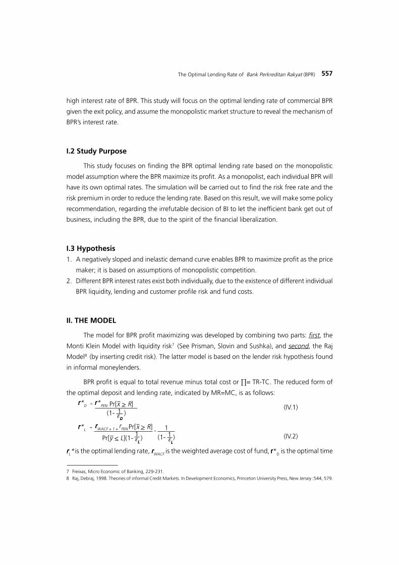
BPR profit is equal to total revenue minus total cost or ∏= TR-TC. The reduced form of

the optimal deposit and lending rate, indicated by MR=MC, is as follows:

(IV.1)

(IV.2)

rrrrrL* is the optimal lending rate, rrrrrWACF is the weighted average cost of fund, rrrrr*D is the optimal time

7 Freixas, Micro Economic of Banking, 229-231.8 Raj, Debraj, 1998. Theories of informal Credit Markets. In Development Economics, Princeton University Press, New Jersey :544, 579.

rrrrr*D = rrrrr*PEN Pr[x > R]

εDDDDD

1(1- )

rrrrr*L=

-rrrrrWACF + 1 + rPEN

Pr[y < L](1- )1ε

LLLLL

11ε

LLLLL

Pr[x > R]

(1- )


deposit rate, rrrrr*S is the optimal saving rate, r*IBL is the optimal inter-bank rate and rrrrr*NBL is the

optimal non bank rate, which is implicit within the rrrrrWACF . The penalty rate from liquidity shortage

is rrrrrPEN , is the probability of the amount of lending that exceeds the reserve requirement

R, and is the probability of credit to not default, while is the Lerner monopoly power,

and εL and εD are correspondingly the elasticity demand for credit and elasticity supply of deposit

( the detail of this model can be seen in the appendix)

Now we will proceed by elaborating the following results such as seen below.

1. If the weight of the bank penalty for the soundness rate for liquidity or rrrrrPEN increases as well

as liquidity risk , the credit rate rrrrrL* and deposit rate rrrrrD* also increase. Consequently

the volume of credit L decreases and the volume of deposit D increases.

2. If the probability of credit default or NPL increases, the probability of credit success or Pr[y < L]

decreases, then the rates rrrrrL* will increase.

II.1 Data

This research uses two different levels of aggregation. First, the BPR individual bank sample

in Jabotabek, covering 41 of 349 BPR in this area; second, the aggregate BPR data, covering all

the 2.228 BPR in Indonesia. The aggregated data are categorized in 43 regional office of BI.

We utilize the information provided in income statement and the balance sheet of the

BPR to asses their performance and Sakernas data to proxy the customer profile including their

aggregate demand. To see regional uniqueness, the RGDP, regional expensiveness index,

consumption pattern and poverty data were obtained from the National Bureau of Statistics

(BPS) and further calculated by LPEM-FEUI. Exclusion is made for the crisis years of 1997 and

1998 to avoid structural breaks that disturb the proper calculation of the optimal lending rate.

The annual data is used from 1996-2002 in Jabotabek and from 1994-2002 in KBI (Regional

Office of Bank Indonesia).

II.2 Rule of Thumb Calculation for BPR Lending Rate

According to Perbarindo calculation9 , the interest rate formation in BPR consists of four

elements: (1) the cost of fund or COF; (2) overhead cost or OHC; (3) risk premium or RISK and

(4) profit margin or PROFIT. The rule of thumb formula (based on accounting principle) for BPR

lending rate is as follows:

COF + OHC + RISK + PROFIT = 100% ºººººººº (IV.5.1a)

1ε

L

9 Interview with pak Dean from Perbarindo

Pr[x > R]

Pr[y < L]

Pr[x > R]

Pr[y < L]


10 The system is also developed by using SUR to find the optimal lending rate of individual BPR in Jabotabek as well as the aggregateBPR in KBI. But these models are not considered as the best model for these areas

11 Unlike the OLS-JBTB and SUR-JBTB models in which the elements of the dummy place are omitted due to the lower level ofsignificance and also lowering the degree of freedom,

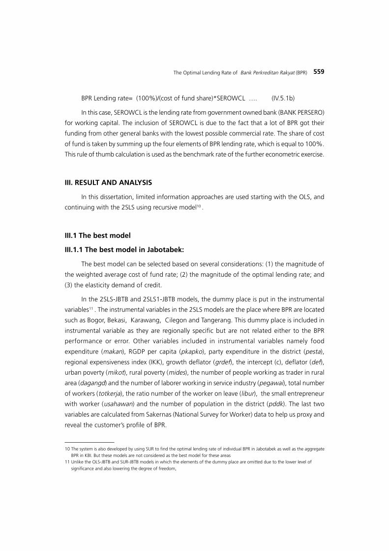
BPR Lending rate= (100%)/(cost of fund share)*SEROWCL º. (IV.5.1b)

In this case, SEROWCL is the lending rate from government owned bank (BANK PERSERO)

for working capital. The inclusion of SEROWCL is due to the fact that a lot of BPR got their

funding from other general banks with the lowest possible commercial rate. The share of cost

of fund is taken by summing up the four elements of BPR lending rate, which is equal to 100%.

This rule of thumb calculation is used as the benchmark rate of the further econometric exercise.

III. RESULT AND ANALYSIS

In this dissertation, limited information approaches are used starting with the OLS, and

continuing with the 2SLS using recursive model10 .

III.1 The best model

III.1.1 The best model in Jabotabek:

The best model can be selected based on several considerations: (1) the magnitude of

the weighted average cost of fund rate; (2) the magnitude of the optimal lending rate; and

(3) the elasticity demand of credit.

In the 2SLS-JBTB and 2SLS1-JBTB models, the dummy place is put in the instrumental

variables11 . The instrumental variables in the 2SLS models are the place where BPR are located

such as Bogor, Bekasi, Karawang, Cilegon and Tangerang. This dummy place is included in

instrumental variable as they are regionally specific but are not related either to the BPR

performance or error. Other variables included in instrumental variables namely food

expenditure (makan), RGDP per capita (pkapko), party expenditure in the district (pesta),

regional expensiveness index (IKK), growth deflator (grdef), the intercept (c), deflator (def),

urban poverty (mikot), rural poverty (mides), the number of people working as trader in rural

area (dagangd) and the number of laborer working in service industry (pegawai), total number

of workers (totkerja), the ratio number of the worker on leave (libur), the small entrepreneur

with worker (usahawan) and the number of population in the district (pddk). The last two

variables are calculated from Sakernas (National Survey for Worker) data to help us proxy and

reveal the customer»s profile of BPR.


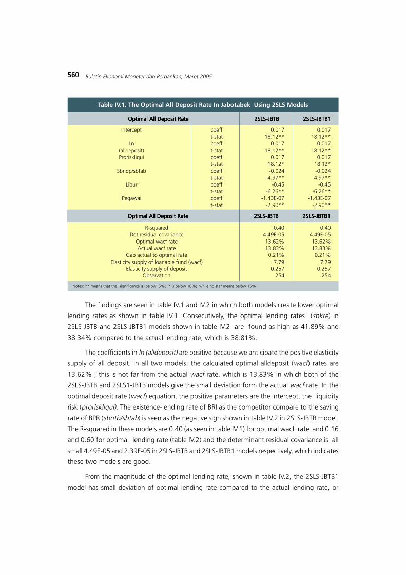
The findings are seen in table IV.1 and IV.2 in which both models create lower optimal

lending rates as shown in table IV.1. Consecutively, the optimal lending rates (sbkre) in

2SLS-JBTB and 2SLS-JBTB1 models shown in table IV.2 are found as high as 41.89% and

38.34% compared to the actual lending rate, which is 38.81%.

The coefficients in ln (alldeposit) are positive because we anticipate the positive elasticity

supply of all deposit. In all two models, the calculated optimal alldeposit (wacf) rates are

13.62% ; this is not far from the actual wacf rate, which is 13.83% in which both of the

2SLS-JBTB and 2SLS1-JBTB models give the small deviation form the actual wacf rate. In the

optimal deposit rate (wacf) equation, the positive parameters are the intercept, the liquidity

risk (proriskliqui). The existence-lending rate of BRI as the competitor compare to the saving

rate of BPR (sbritb/sbtab) is seen as the negative sign shown in table IV.2 in 2SLS-JBTB model.

The R-squared in these models are 0.40 (as seen in table IV.1) for optimal wacf rate and 0.16

and 0.60 for optimal lending rate (table IV.2) and the determinant residual covariance is all

small 4.49E-05 and 2.39E-05 in 2SLS-JBTB and 2SLS-JBTB1 models respectively, which indicates

these two models are good.

From the magnitude of the optimal lending rate, shown in table IV.2, the 2SLS-JBTB1

model has small deviation of optimal lending rate compared to the actual lending rate, or

Table IV.1. The Optimal All Deposit Rate In Jabotabek Using 2SLS Models

Notes: ** means that the significance is below 5%; * is below 10%; while no star means below 15%

Intercept coeff 0.017 0.017t-stat 18.12** 18.12**

Ln coeff 0.017 0.017(alldeposit) t-stat 18.12** 18.12**Proriskliqui coeff 0.017 0.017

t-stat 18.12* 18.12*Sbridp/sbtab coeff -0.024 -0.024

t-stat -4.97** -4.97**Libur coeff -0.45 -0.45

t-stat -6.26** -6.26**Pegawai coeff -1.43E-07 -1.43E-07

t-stat -2.90** -2.90**

Optimal All Deposit RateOptimal All Deposit RateOptimal All Deposit RateOptimal All Deposit RateOptimal All Deposit Rate 2SLS-JBTB2SLS-JBTB2SLS-JBTB2SLS-JBTB2SLS-JBTB 2SLS-JBTB12SLS-JBTB12SLS-JBTB12SLS-JBTB12SLS-JBTB1

Optimal All Deposit RateOptimal All Deposit RateOptimal All Deposit RateOptimal All Deposit RateOptimal All Deposit Rate 2SLS-JBTB2SLS-JBTB2SLS-JBTB2SLS-JBTB2SLS-JBTB 2SLS-JBTB12SLS-JBTB12SLS-JBTB12SLS-JBTB12SLS-JBTB1

R-squared 0.40 0.40Det.residual covariance 4.49E-05 4.49E-05

Optimal wacf rate 13.62% 13.62%Actual wacf rate 13.83% 13.83%

Gap actual to optimal rate 0.21% 0.21%Elasticity supply of loanable fund (wacf) 7.79 7.79

Elasticity supply of deposit 0.257 0.257Observation 254 254


38.34% compare to 38.81%. From the T-statistic appearance from each variable, we have the

best overall picture in 2SLS-JBTB1 compared to the other models, in which all of variables have

T-stat significance below 5% level, except for the intercept and sbrikr (BRI lending rate) variables,

which are below 10% level of significance. From the elasticity demand of credit, only these two

models create relatively the inelastic demand curve -1.748 and √2.523 compare to the case of

the Philippine»s farmer demand12 . These relatively inelastic nature of debtor»s demand in 2SLS

models confirm the assumption of monopolistic competition.

III.1.2 The Best Model in KBI

When KBI aggregate data are runned, the OLS-KBI, and OLS-KBI1 is selected as the

good models. Because the smallest gap in wacf rate and the inelastic nature of the demand

for credits is found in the OLS-KBI1 model, hence, it is considered as the best model.

In OLS-KBI1 model, we are able to see the overall factors, including the monetary

intervention and linkage program. The OLS-KBI model is used as the benchmark for the

Table IV.2. The Optimal Lending Rate In Jabotabek Using 2SLS Models

R-squaredR-squaredR-squaredR-squaredR-squared 0.1654 0.60Optimal lending rate 41.89% 38.34%Actual lending rate 38.81% 38.81%

Gap optimal-actual rate -3.08% 0.47%Elasticity demand for credit -1.748 -2.523

InterceptInterceptInterceptInterceptIntercept coeff 0.3186 0.280t-stat 3.73** 3.25**

Ln (Tkred/ totas) coeff -0.2012 -0.15t-stat -2.49** -2.67**

npl coeff 0.3258 0.280t-stat 4.034** 3.25**

Wacf coeff 1.204 1.022t-stat 2.72** 3.53**

Makan/pesta coeff 0.004 0.00035t-stat 1.93** 2.24**

Sbrikr/sbtab coeff -0.035t-stat -2.22**

Pdkokap/ikk coeff -3.119t-stat -1.801**

Intervene coeff -0.3068t-stat -2.26**


Optimal Lending rateOptimal Lending rateOptimal Lending rateOptimal Lending rateOptimal Lending rate 2SLS-JBTB2SLS-JBTB2SLS-JBTB2SLS-JBTB2SLS-JBTB 2SLS-JBTB12SLS-JBTB12SLS-JBTB12SLS-JBTB12SLS-JBTB1

Optimal Lending rateOptimal Lending rateOptimal Lending rateOptimal Lending rateOptimal Lending rate 2SLS-JBTB2SLS-JBTB2SLS-JBTB2SLS-JBTB2SLS-JBTB 2SLS-JBTB12SLS-JBTB12SLS-JBTB12SLS-JBTB12SLS-JBTB1

12 Based on the study of Briones Roehlo (2000)


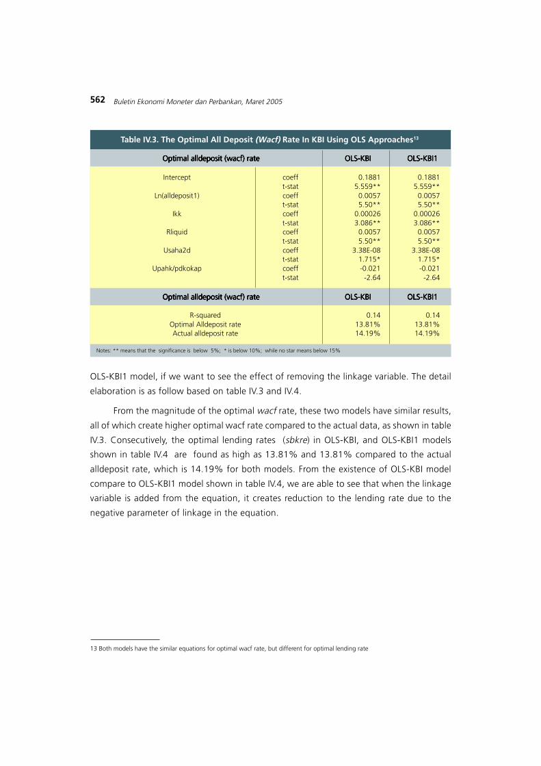
OLS-KBI1 model, if we want to see the effect of removing the linkage variable. The detail

elaboration is as follow based on table IV.3 and IV.4.

From the magnitude of the optimal wacf rate, these two models have similar results,

all of which create higher optimal wacf rate compared to the actual data, as shown in table

IV.3. Consecutively, the optimal lending rates (sbkre) in OLS-KBI, and OLS-KBI1 models

shown in table IV.4 are found as high as 13.81% and 13.81% compared to the actual

alldeposit rate, which is 14.19% for both models. From the existence of OLS-KBI model

compare to OLS-KBI1 model shown in table IV.4, we are able to see that when the linkage

variable is added from the equation, it creates reduction to the lending rate due to the

negative parameter of linkage in the equation.

Table IV.3. The Optimal All Deposit (Wacf) Rate In KBI Using OLS Approaches13

R-squared 0.14 0.14Optimal Alldeposit rate 13.81% 13.81%Actual alldeposit rate 14.19% 14.19%

Intercept coeff 0.1881 0.1881t-stat 5.559** 5.559**

Ln(alldeposit1) coeff 0.0057 0.0057t-stat 5.50** 5.50**

Ikk coeff 0.00026 0.00026t-stat 3.086** 3.086**

Rliquid coeff 0.0057 0.0057t-stat 5.50** 5.50**

Usaha2d coeff 3.38E-08 3.38E-08t-stat 1.715* 1.715*

Upahk/pdkokap coeff -0.021 -0.021t-stat -2.64 -2.64


Optimal alldeposit (wacf) rateOptimal alldeposit (wacf) rateOptimal alldeposit (wacf) rateOptimal alldeposit (wacf) rateOptimal alldeposit (wacf) rate OLS-KBIOLS-KBIOLS-KBIOLS-KBIOLS-KBI OLS-KBI1OLS-KBI1OLS-KBI1OLS-KBI1OLS-KBI1

Optimal alldeposit (wacf) rateOptimal alldeposit (wacf) rateOptimal alldeposit (wacf) rateOptimal alldeposit (wacf) rateOptimal alldeposit (wacf) rate OLS-KBIOLS-KBIOLS-KBIOLS-KBIOLS-KBI OLS-KBI1OLS-KBI1OLS-KBI1OLS-KBI1OLS-KBI1

13 Both models have the similar equations for optimal wacf rate, but different for optimal lending rate


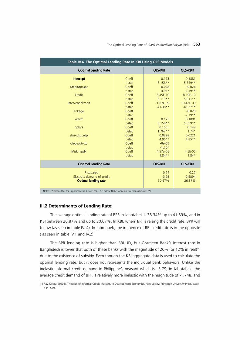
III.2 Determinants of Lending Rate:

The average optimal lending rate of BPR in Jabotabek is 38.34% up to 41.89%, and in

KBI between 26.87% and up to 30.67%. In KBI, when BRI is raising the credit rate, BPR will

follow (as seen in table IV. 4). In Jabotabek, the influence of BRI credit rate is in the opposite

( as seen in table IV.1 and IV.2).

The BPR lending rate is higher than BRI-UD, but Grameen Bank»s interest rate in

Bangladesh is lower that both of these banks with the magnitude of 20% (or 12% in real)14

due to the existence of subsidy. Even though the KBI aggregate data is used to calculate the

optimal lending rate, but it does not represents the individual bank behaviors. Unlike the

inelastic informal credit demand in Philippine»s peasant which is √5.79; in Jabotabek, the

average credit demand of BPR is relatively more inelastic with the magnitude of -1.748, and

Table IV.4. The Optimal Lending Rate In KBI Using OLS Models

R-squared 0.24 0.27Elasticity demand of credit -3.93 -0.5894

Optimal lending rateOptimal lending rateOptimal lending rateOptimal lending rateOptimal lending rate 30.67% 26.87%

InterceptInterceptInterceptInterceptIntercept Coeff 0.173 0.1881t-stat 5.158** 5.559**

Kredit/toaspr Coeff -0.028 -0.024t-stat -4.95* -2.19**

kredit Coeff 8.45E-10 8.19E-10t-stat 5.119** 5.011**

Intervene*kredit Coeff -1.67E-09 -1.642E-09t-stat -4.638** -4.627**

linkage Coeff -0.028t-stat -2.19**

wacff Coeff 0.173 0.1881t-stat 5.158** 5.559**

nplgrs Coeff 0.1535 0.149t-stat 1.767** 1.74*

sbrikr/sbprdp Coeff 0.0228 0.0221t-stat 4.95** 4.85**

otrckr/otrctb Coeff -8e-05t-stat -1.70*

Miskin/pdk Coeff 4.57e-05 4.5E-05t-stat 1.84** 1.84*


Optimal Lending RateOptimal Lending RateOptimal Lending RateOptimal Lending RateOptimal Lending Rate OLS-KBIOLS-KBIOLS-KBIOLS-KBIOLS-KBI OLS-KBI1OLS-KBI1OLS-KBI1OLS-KBI1OLS-KBI1

Optimal Lending RateOptimal Lending RateOptimal Lending RateOptimal Lending RateOptimal Lending Rate OLS-KBIOLS-KBIOLS-KBIOLS-KBIOLS-KBI OLS-KBI1OLS-KBI1OLS-KBI1OLS-KBI1OLS-KBI1

14 Ray, Debraj (1998), Theories of Informal Credit Markets. In Development Economics, New Jersey: Princeton University Press, page544, 579.


15 Econometrically this fact exist if conjectural variations _ (the reaction function of the firm as those developed by Cournot oligopolisticmodel) is equal one, hence from the equation (P-MC)/P= (_+ (1-_) H)/_ the equation (P-MC)/P=1/_. will be found. In this case H isthe Herfindahl index for the market concentration.

16 In which consecutively 8.23 %, 0.01% and 2.87% came from the credit risk, liquidity risk and consumer profile risk.17 As those elaborated by Padmanabhan18 In E views software, the log expression means Ln (natural logarithmic)

the Lerner monopoly index15 is equal to 0.572. In KBI assessment, credit demand elasticity in

BPR is -0.589 with monopoly index equal to 1.69. This strengthens the monopolistic competition

and loyalty of the BPR debtors for those located in the big cities. From 100% BPR»s interest

rate, the total risk components from rule of thumb calculation that use accounting principle is

33,70%, but from econometric assessment16 the risk components are around 11.28% to

25.08% in Jabotabek and 9.21% up to 27.41% in KBI. These discrepancies are due to errors

in econometric exercises. The missing variables that make the risk components appear smaller.

It is seen that small and economically weak group in poor areas have to pay higher

interest rate because BPR sees them as the riskier customers. The proponents of the old

paradigm17 often use this finding to criticize BPR for being merciless to the poor people.

Undeniably for the sake of business sustainability, to resist the peril of bankruptcy, there is no

other choice except for maximizing its profit.

III.2.1 in Jabotabek

The most important distinction between 2SLS-JBTB and 2SLS-JBTB1 is the inclusion of

variable intervene (BI liquidity program) and the exclusion of non-significant variable sbrikr/

sbtab in 2SLS-JBTB1 model. This higher predicted rate 41.89% in 2SLS-JBTB compares to the

actual rate 38.81% does not mean that the missing variable (with positive direction of

parameters) problem is absent or decreasing. It is due to the opposite direction of bias. The

lower predicted lending rate 38.34% in 2SLS-JBTB1 compares to the actual rate 38.81% means

that the missing variables exist. When we compare the elasticity demand of credit using 2SLS

approach, the relatively most inelastic demand -1.748 is found in 2SLS-JBTB model and the

second one √2.523 is found in 2SLS-JBTB1 model. It seems that when BI creates liquidity

program to BPR, the intervene variable, not only the interest rate of BPR is lower, but also the

more elastic demand of credit is emerged.

In 2SLS model, the gap between calculated optimal lending rate 41.89% and the actual

lending rate 38.81% is 3.05%. In 2SLS-JBTB1 model the gap is only 0.47% , which makes

the 2SLS-JBTB1 model the best model in terms of lending rate. In this model, the intercept

parameter of optimal lending rate is 0.28, and the total amount of credit in natural logarithm

ln(tkred/totas) in the district18 creates negative parameter. The elasticity demand of credit


19 this is calculated by R. Briones (2002)20 As those elaborated by Stephen Martin

equals to -2.523. In 2SLS-JBTB1 the elasticity demand of credit is -1.748. This number is

also more inelastic compare to the Philippine rice farmer demand for informal lending,

which is -5.7919 . This elasticity demand of credit is on par with our assumption about the

monopolistic nature of BPR customers. Monopolistic competition is situated between perfect

monopoly and perfect competition in which the negatively sloped demand curve exists.

The slope is not exactly equal to zero such as in perfectly inelastic demand or equal to ~

(infinity) such as in perfect competition. Hence, the 2SLS1-JBTB model is the best model in

Jabotabek in terms of representing the most inelastic demand of credit -1.748 that reflecting

the more loyal customer compare to the other models. The R-squared in 2SLS-JBTB1 model

also good as high as 0.60.

In optimal lending rate equation of 2SLS-JBTB1 model as seen in table IV.4, the

magnitudes of credit risk (npl) parameter as well as the weighted average cost of fund

(wacf) rates are consecutively 0.280 and 1.022, which means that the higher the credit risk

(npl) and the weighted average cost of fund (wacf), the higher the optimal lending rate.

The interesting thing is the existence of the ratio of BRI lending to BPR saving rate (sbrikr/

sbtab) in 2SLS-JBTB, which creates negative parameter in BPR lending rate, with significant

level is below 5%. It means that BRI becomes the strategic substitute of BPR20 . Every time

BRI increases the lending rate compared to the BPR saving rate, BPR will reduce the lending

rate. But in 2SLS-JBTB1 model, when variable BI liquidity program intervene is put inside

the equation, this BRI lending rate variable is not significant; hence it is omitted.

The customers» profiles safety (as the opposite of risk) are also reflected in the 2SLS-

JBTB and 2SLS-JBTB1 model, which is captured through the worker on leave in the district

or the (libur) variable and the workers working at the service sector (pegawai), which has

negative sign and significance below 5%. The richer the area as reflected from the per

capita RGDP divided by consumer»s price index (pdkokap/ikk) the less the lending rate in

2SLS-JBTB model. It means that the more the economically weak group working in service

sector, or able to take a leave, or working in richer area, the lower the lending rate of BPR.

The optimal lending rate of BPR in 2SLS-JBTB and 2SLS-JBTB1 models is 38.34%, which is

not far from the actual BPR rate, 38.81%. This lower predicted rate compare to the actual

data is due to missing positive variables.


III.2.2 in KBI:

The optimal lending rates (sbkre) in the OLS-KBI and OLS-KBI1 models shown in table

IV.4 are 30.67% and 26.96% respectively compared to the actual lending rate, which is 31.12%.

Hence, the missing variables create positive gaps in these two models.

On the other hand, the T-statistics from the OLS-KBI model are significant which give the

good overall picture of this model, in which the majority of parameters have T-statistic below

5% significance level, except the parameter of usaha2d or the small entrepreneur in rural area,

the nplgrs or non performing loan, and miskin/pdk or the ratio of people under poverty line

compare to total population in the district which are below 10% significance level.

In this case we have negative parameter of total credit per total asset of BPR or kredit/

toaspr, which represents the negative elasticity demand of credit. The reason why we divide

total credit by total asset is to see the portfolio of BPR asset and to proxy the risk-related

weights for the computation of the capital to asset ratio21 . The main idea is that if banks

behave as portfolio managers when they choose the composition of their portfolio of assets

and liabilities, this risk-related weight is very important to be considered22 . The larger the ratio

of credit compares to total asset in KBI, the smaller the lending rate because BPR able to create

bigger economic of scale and the elasticity demand of credit is negative. In this case, because

asset is the denumerator and based on the law of large number, the bigger the BPR asset, the

better for BPR to create portfolio of risk when performing their intermediary function. Hence,

the interest rate is also reduced. Other variable that is able to reduce the lending rate as seen in

table IV.4 is the amount of interbank loan compare to total credit or linkage variable which is

seen in OLS-KBI1 model, in which the larger the linkage variable; therefore, the smaller the

lending rate. In these models, the optimal weighted average cost of fund or wacf creates

higher interest rate, and the higher the non-performing loan such as seen in nplgrs variable,

the higher the lending rate.

The ratio of BRI lending rate compared to BRI deposit rate or sbrikr/sbridp creates positive

impact on the BPR lending rate in all KBI models, which means that BRI becomes the market

leader of BPR23 . Every time BRI increases the lending rate, BPR will follow BRI in increasing the

lending rate as well. This is in line with the mathematical model originated from the lender»s

risk hypothesis in which the formal sector rate becomes the benchmark of informal sector

(BPR) rate.

21 In Indonesia, this regulation is based on the BI director»s decision number 26/20/KEP/DIR about the minimum requirements of bankcapital and the circulating letter of Bank Indonesia number 26/2/BPPP for the case of BPR

22 Freixas, 2002, this is also in line with the Stiglitz and Greenwald book about the new monetary economic.23 As those elaborated by Stephen Martin


In OLS-KBI and OLS-KBI1 models we find that the customer profile risk is expressed by

the number of people under poverty line per total population or miskin/pdk as seen in the last

components of optimal lending rate (shown in table IV.4) that creates increasing impact on the

lending rate. It means that the economically weak group and the small and medium entrepreneur

in poor area create higher BPR interest rate.

To see the impact of intervention to reduce lending rate, in table IV.4. In OLS-KBI1 model

we are able to prove that the BI liquidity program intervene*kredit variable as the policy

intervention24 of the monetary authority is able to reduce lending rate based on the negative

parameters of the model. The only different elements between OLS-KBI model and OLS-KBI1

model is the linkage elements as the BPR»s networking effort to reach bigger economic of scale

and economic of scope, and are able to reduce the lending rate of BPR to 26.96% that creates

inelastic demand for credit -0.5894.

III.3 The Elasticity:

The elements of total loanable fund are the time deposits, savings, inter bank liabilities,

non-bank liabilities and BI liabilities. In table IV.5 we do not calculate the elasticity supply of BI

liability, because the BI liquidity program is only temporary even though the BPR liabilities to BI are

still shown until the Year 2002. The first two elements, the time deposit and saving, will create

the calculation of the elasticity supply of time deposit, as well as the elasticity supply of saving.

III.3.1 In Jabotabek

These elasticities of the alldeposit components are anticipated to be positive in sign,

except maybe for saving. There is a tendency that the BPR savers in Jabotabek are coerced to

save if they want to become the BPR debtors. In several big BPRs in Jabotabek, during surveys,

it is also found that all debtors are also compelled to join the credit insurance. Therefore, in

Jabotabek, there is no voluntary saving, which is anticipated to create confusing sign of the

elasticity supply of saving25 . The negative sign of this elasticity -2.339 reflects this. It means that

even though BPR is reducing the saving rate, the BPR»s savers are not lessening their saving in

BPR. Moreover, for the sake of their anxious demand of credit, the saving rate consideration is

not important.

24 The liquidity program was designed only during emergency situation. Even though it is stopped because the crisis is over, but theBPR liability to BI still exists during time observation (interview with BI staff).

25 In voluntary saving, the elasticity supply of deposit must be positive, because if the saving rate is higher than the amount of savingwill be higher. But in BPR case, because the aim of the saver is not gaining the revenue from saving rate, but obtaining the credit, thenormal elasticity supply of saving will not be performed.


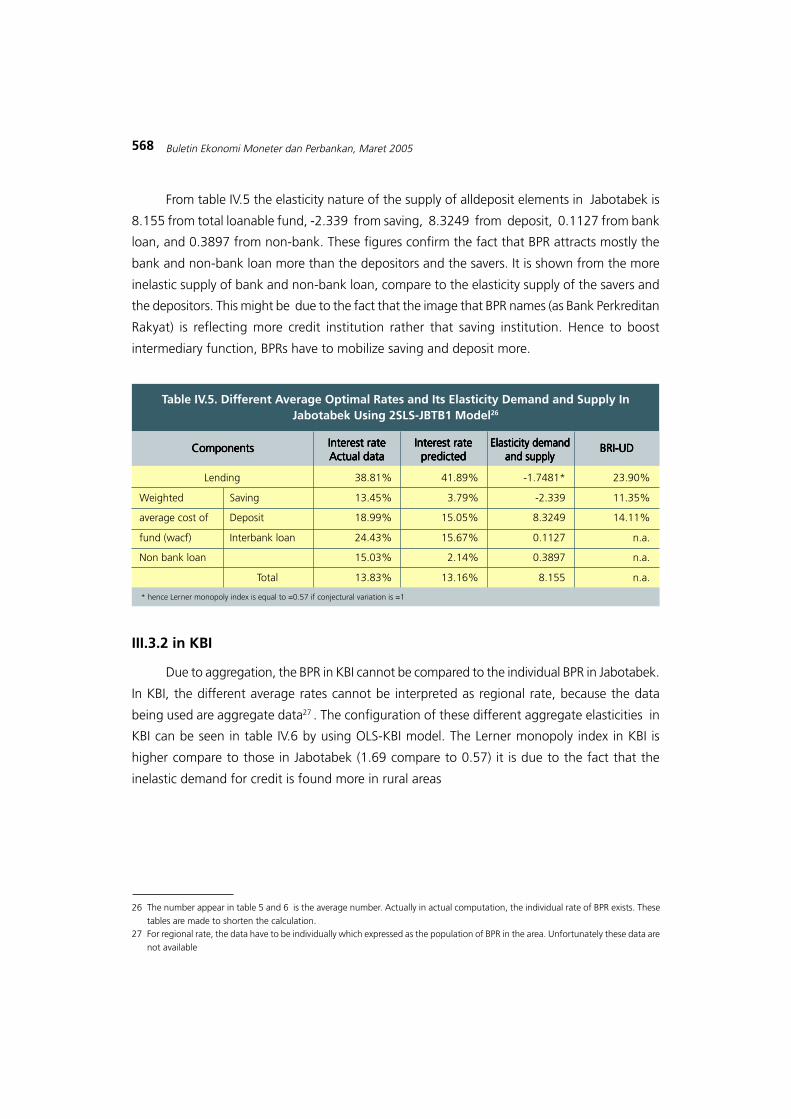
From table IV.5 the elasticity nature of the supply of alldeposit elements in Jabotabek is

8.155 from total loanable fund, -2.339 from saving, 8.3249 from deposit, 0.1127 from bank

loan, and 0.3897 from non-bank. These figures confirm the fact that BPR attracts mostly the

bank and non-bank loan more than the depositors and the savers. It is shown from the more

inelastic supply of bank and non-bank loan, compare to the elasticity supply of the savers and

the depositors. This might be due to the fact that the image that BPR names (as Bank Perkreditan

Rakyat) is reflecting more credit institution rather that saving institution. Hence to boost

intermediary function, BPRs have to mobilize saving and deposit more.

Table IV.5. Different Average Optimal Rates and Its Elasticity Demand and Supply InJabotabek Using 2SLS-JBTB1 Model26

ComponentsComponentsComponentsComponentsComponents

Lending 38.81% 41.89% -1.7481* 23.90%

Weighted Saving 13.45% 3.79% -2.339 11.35%

average cost of Deposit 18.99% 15.05% 8.3249 14.11%

fund (wacf) Interbank loan 24.43% 15.67% 0.1127 n.a.

Non bank loan 15.03% 2.14% 0.3897 n.a.

Total 13.83% 13.16% 8.155 n.a.

Interest rateInterest rateInterest rateInterest rateInterest rateActual dataActual dataActual dataActual dataActual data

Interest rateInterest rateInterest rateInterest rateInterest ratepredictedpredictedpredictedpredictedpredicted

Elasticity demandElasticity demandElasticity demandElasticity demandElasticity demandand supplyand supplyand supplyand supplyand supply

BRI-UDBRI-UDBRI-UDBRI-UDBRI-UD

* hence Lerner monopoly index is equal to =0.57 if conjectural variation is =1

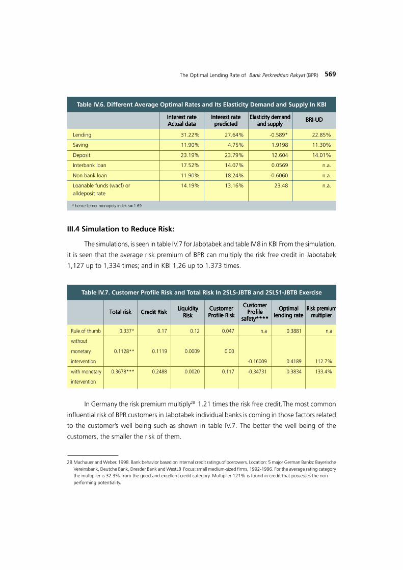
III.3.2 in KBI

Due to aggregation, the BPR in KBI cannot be compared to the individual BPR in Jabotabek.

In KBI, the different average rates cannot be interpreted as regional rate, because the data

being used are aggregate data27 . The configuration of these different aggregate elasticities in

KBI can be seen in table IV.6 by using OLS-KBI model. The Lerner monopoly index in KBI is

higher compare to those in Jabotabek (1.69 compare to 0.57) it is due to the fact that the

inelastic demand for credit is found more in rural areas

26 The number appear in table 5 and 6 is the average number. Actually in actual computation, the individual rate of BPR exists. Thesetables are made to shorten the calculation.

27 For regional rate, the data have to be individually which expressed as the population of BPR in the area. Unfortunately these data arenot available


Table IV.6. Different Average Optimal Rates and Its Elasticity Demand and Supply In KBI

Lending 31.22% 27.64% -0.589* 22.85%

Saving 11.90% 4.75% 1.9198 11.30%

Deposit 23.19% 23.79% 12.604 14.01%

Interbank loan 17.52% 14.07% 0.0569 n.a.

Non bank loan 11.90% 18.24% -0.6060 n.a.

Loanable funds (wacf) or 14.19% 13.16% 23.48 n.a.alldeposit rate

Interest rateInterest rateInterest rateInterest rateInterest rateActual dataActual dataActual dataActual dataActual data

Interest rateInterest rateInterest rateInterest rateInterest ratepredictedpredictedpredictedpredictedpredicted

Elasticity demandElasticity demandElasticity demandElasticity demandElasticity demandand supplyand supplyand supplyand supplyand supply

BRI-UDBRI-UDBRI-UDBRI-UDBRI-UD

* hence Lerner monopoly index is= 1.69

28 Machauer and Weber. 1998. Bank behavior based on internal credit ratings of borrowers. Location: 5 major German Banks: BayerischeVereinsbank, Deutche Bank, Dresder Bank and WestLB Focus: small medium-sized firms, 1992-1996. For the average rating categorythe multiplier is 32.3% from the good and excellent credit category. Multiplier 121% is found in credit that possesses the non-performing potentiality.

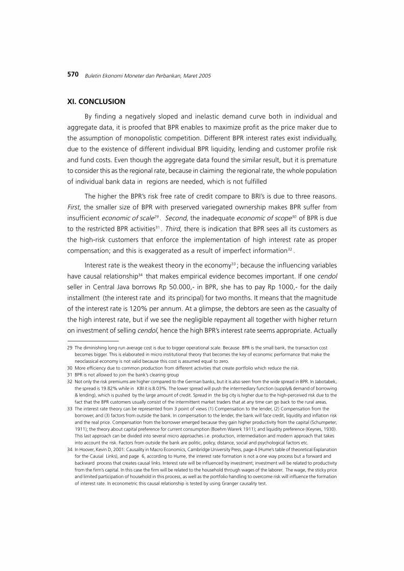
III.4 Simulation to Reduce Risk:

The simulations, is seen in table IV.7 for Jabotabek and table IV.8 in KBI From the simulation,

it is seen that the average risk premium of BPR can multiply the risk free credit in Jabotabek

1,127 up to 1,334 times; and in KBI 1,26 up to 1.373 times.

Table IV.7. Customer Profile Risk and Total Risk In 2SLS-JBTB and 2SLS1-JBTB Exercise

Rule of thumb 0.337* 0.17 0.12 0.047 n.a 0.3881 n.a

without

monetary 0.1128** 0.1119 0.0009 0.00

intervention -0.16009 0.4189 112.7%

with monetary 0.3678*** 0.2488 0.0020 0.117 -0.34731 0.3834 133.4%

intervention

Total riskTotal riskTotal riskTotal riskTotal risk Credit RiskCredit RiskCredit RiskCredit RiskCredit RiskLiquidityLiquidityLiquidityLiquidityLiquidity

RiskRiskRiskRiskRiskCustomerCustomerCustomerCustomerCustomerProfile RiskProfile RiskProfile RiskProfile RiskProfile Risk

CustomerCustomerCustomerCustomerCustomerProfileProfileProfileProfileProfile

safety****safety****safety****safety****safety****

OptimalOptimalOptimalOptimalOptimallending ratelending ratelending ratelending ratelending rate

Risk premiumRisk premiumRisk premiumRisk premiumRisk premiummultipliermultipliermultipliermultipliermultiplier

In Germany the risk premium multiply28 1.21 times the risk free credit.The most common

influential risk of BPR customers in Jabotabek individual banks is coming in those factors related

to the customer»s well being such as shown in table IV.7. The better the well being of the

customers, the smaller the risk of them.


XI. CONCLUSION

By finding a negatively sloped and inelastic demand curve both in individual and

aggregate data, it is proofed that BPR enables to maximize profit as the price maker due to

the assumption of monopolistic competition. Different BPR interest rates exist individually,

due to the existence of different individual BPR liquidity, lending and customer profile risk

and fund costs. Even though the aggregate data found the similar result, but it is premature

to consider this as the regional rate, because in claiming the regional rate, the whole population

of individual bank data in regions are needed, which is not fulfilled

The higher the BPR»s risk free rate of credit compare to BRI»s is due to three reasons.

First, the smaller size of BPR with preserved variegated ownership makes BPR suffer from

insufficient economic of scale29 . Second, the inadequate economic of scope30 of BPR is due

to the restricted BPR activities31 . Third, there is indication that BPR sees all its customers as

the high-risk customers that enforce the implementation of high interest rate as proper

compensation; and this is exaggerated as a result of imperfect information32 .

Interest rate is the weakest theory in the economy33 ; because the influencing variables

have causal relationship34 that makes empirical evidence becomes important. If one cendol

seller in Central Java borrows Rp 50.000,- in BPR, she has to pay Rp 1000,- for the daily

installment (the interest rate and its principal) for two months. It means that the magnitude

of the interest rate is 120% per annum. At a glimpse, the debtors are seen as the casualty of

the high interest rate, but if we see the negligible repayment all together with higher return

on investment of selling cendol, hence the high BPR»s interest rate seems appropriate. Actually

29 The diminishing long run average cost is due to bigger operational scale. Because BPR is the small bank, the transaction costbecomes bigger. This is elaborated in micro institutional theory that becomes the key of economic performance that make theneoclassical economy is not valid because this cost is assumed equal to zero.

30 More efficiency due to common production from different activities that create portfolio which reduce the risk.31 BPR is not allowed to join the bank»s clearing group32 Not only the risk premiums are higher compared to the German banks, but it is also seen from the wide spread in BPR. In Jabotabek,

the spread is 19.82% while in KBI it is 8.03%. The lower spread will push the intermediary function (supply& demand of borrowing& lending), which is pushed by the large amount of credit. Spread in the big city is higher due to the high-perceived risk due to thefact that the BPR customers usually consist of the intermittent market traders that at any time can go back to the rural areas.

33 The interest rate theory can be represented from 3 point of views (1) Compensation to the lender, (2) Compensation from theborrower, and (3) factors from outside the bank. In compensation to the lender, the bank will face credit, liquidity and inflation riskand the real price. Compensation from the borrower emerged because they gain higher productivity from the capital (Schumpeter,1911); the theory about capital preference for current consumption (Boehm Warerk 1911); and liquidity preference (Keynes, 1930).This last approach can be divided into several micro approaches i.e. production, intermediation and modern approach that takesinto account the risk. Factors from outside the bank are politic, policy, distance, social and psychological factors etc.

34 In Hoover, Kevin D, 2001: Causality in Macro Economics, Cambridge University Press, page 4 (Hume»s table of theoretical Explanationfor the Causal Links), and page 6, according to Hume, the interest rate formation is not a one way process but a forward andbackward process that creates causal links. Interest rate will be influenced by investment; investment will be related to productivityfrom the firm»s capital. In this case the firm will be related to the household through wages of the laborer. The wage, the sticky priceand limited participation of household in this process, as well as the portfolio handling to overcome risk will influence the formationof interest rate. In econometric this causal relationship is tested by using Granger causality test.


the main reason of the debtors when borrow from BPR is not the interest rate, but to gain

easy access to the small and uncomplicated credit35 . The formula of interest rate is too naive

that hide the amount of credit, return on investment, risk premium, risk sharing, search cost

and illiquidity factor. Unfortunately the discussions about interest rate often neglect these

aspects, especially if the discussion is motivated more by the non-economic judgment.

Reducing interest rate of credit according to the new paradigm can be done only

indirectly for example by obtaining cheaper cost of fund. This research found out that deposit

and saving supply of BPR is more elastic compare to BPR»s borrowing from the bank and

non-bank. It means that the attraction of other bank and non-bank in channeling their funding

through BPR is easier and more reliable compare to the saver and depositor funding. This

finding also reflects that saving and deposit mobility in BPR is inadequate. Does it mean that

Boeke»s hypothesis during colonial period36 about credit thirst is true? It is apparent that

even though the role of deposit is not satisfying37 , but the growth and the amount of both

saving and deposit and its accounts are faster and greater compare to those of credit38 .

Based on LPEM√FEUI»s survey about micro finance39 it is found out that respondents wants

more saving and loan institution compare to credit institution with low lending rate. Hence

the Boeke»s hypothesis is wrong40 . In the future BPR»s name that possess profound connotation

as credit rather than saving or deposit institution might be replaced with a proper name to

reflect more effort to mobilize funding from savers and depositors which also reflects prudent

and proper intermediary institution.

The low interest rate of bank and non bank borrowing of BPR41 have potential to reduce

35 Based on Unand and IBI survey in West Sumatra 2002, which was in cooperation with BI. It is found that interest rate is the 11thfactors among 12 alternatives when the debtor»s candidate borrows from BPR.

36 This hypothesis was made by Boeke during colonial period because the indigenous people who were thirsty of credit become thecasualties of Tjina Mindring and Arab moneylender who imposed high interest rate. Because Tjina Mindrings were more numerouscompare to the Arab moneylenders, it gave the Tjina Mindring more awful image. The convenience to collect the high interest creditrepayment is worsened by the involvement of the village officials who worked in cooperation with the Chinese money lender (TjinaMindring) as elaborated by Burger in Kahin»s book about, Nationalism and Revolution in Indonesia, page 9. Based on ethical policyof the Dutch, government has to do something to protect the indigenous people. Between 1920 and 1928 Boeke and Fruin madedistrict bank that became the grand fathered BPR, which were under the supervision of the ministry of Internal Affairs. Then the«Volkscredietwezen» emerged at the year 1929 as the early form of BRI. This is elaborated by Schmit, L.Th. (1991), ≈Rural CreditBetween Subsidy And Market, Adjustment Of The Village Units Of Bank Rakyat Indonesia∆ in Sociological Perspective, LeidenDevelopment Studies, no.11, and page 55-61.

37 From the assessment it is found that the deposit role is 55,27% and from saving it is 25,15% from total loanable fund.38 This is due to in Jabotabek, the deposit rate in BPR is 18.99% higher than BRI 14.11%, and the saving rate is 13.45% higher than

BRI 11.35%. In KBI the BPR»s deposit rate is 23.19% compare to 14.01% BRI UD»s deposit rate, while the BPR»s saving rate is11.90% compare to 11.30% of the BRI-UD»s.

39 Survey was done at 8 provinces in 1997 by LPEM-FEUI that performed this study about Financial Development in several backwardareas in Indonesia.

40 Boeke»s hypothesis is also opposed by Steinwand in his book, The Alchemy of Micro Finance, 2002.41 It consists of 16,41% from inter bank borrowing and 2,10% from total lonable fund of BPR.


BPR interest rate of credit but actually these interest rates are high42 . If BPR belongs to a group,

the interest rate will be lower because the risks are smaller due to the risk spreading.

Unfortunately the group ownership of BPR is prohibited43 , because there is apprehension

that if BPR is getting bigger these banks are no longer willing to access the lower income and

economically weak group44 . If suspicious group ownership of BPR exists, the blame can be

placed due to the adverse selection as a result of the weak regulation and supervision as the

ex-post asymmetric information45 . If BPR ownership in groups is not allowed, the program

linkage such as executing46 or channeling47 is alternative solution to reduce BPR»s interest

rate. Empirically linkage variable able to reduce BPR»s interest rate48 , but in Jabotabek the

findings are not always consistent.

The six Cs debtor»s prerequisite being used by BPR to reduce risk through relationship

marketing49 based on customer»s profile that lengthens the customer»s loyalty create higher

cost per unit of lending. The overhead cost of BPR is about 20% from 100% lending rate.

Other effort to reduce lending rate of BPR can be developed if the information is

disseminated well, so that the BPR debtors can see other sources of credit sources that make

their credit demand becomes more elastic50. It will make BPR loosing its monopolistic power.

Actually, all efforts to reduce lending rate are handed over to the market mechanism to decide

the final rate. The new paradigm does not support the subsidized rate because credit quota will

emerge in which mostly the rich individual attains the subsidized credit. No wonder that the

income distribution is worsened. Moral hazard such as non-performing loan is often found due

to the misperception that this credit is seen as the charity51 . This is not only happened in

Indonesia, but also in Bangladesh, India, Korea and Nepal52 . The subsidized credit has created

42 Borrowing rate from other bank and non-bank consecutively 24.43% and 15.03% in Jabotabek; in KBI the rates are 11.9% and17.52%. The cost of interest is higher in the big city (Jabotabek) compare to KBI because the higher risk is found in the big city.

43 Even though it is prohibited, but BI often receives several proposals to establish BPR in group. Despite this ban, actually BPRownership in group is hard to supervise even though fit and proper tests are developed by BI.

44 Pandu Suharto (1991), in his book Peran, Masalah dan Prospek BPR, Lembaga Pengembangan Perbankan, Indonesia elaboratedone of the BI director.45 There is indication that BPR in group (even though it is prohibited), is still operating, but they are still imposing the highinterest rate. This is due to the inelastic demand of credit. From econometric assessment there is no validity that the bigger BPR thesmaller interest rate.

46 Executing is developed if the credit disbursement is in BPR and is seen in the balance sheet .47 Channeling is formed if credit disbursement responsibility is located outside the BPR, this component is found in the off balance

sheet.48 The linkage variable here is proxied by BPR»s inter bank lending rate repayment. Linkage can be seen in the financial or non-financial

linkage such as in the supervision activities.49 As shown by Leonard Berry50 In Jabotabek (Jakarta, Bogor Tangerang Bekasi), when BNI creates Micro Service Unit in Jakarta with lower interest rate compare to

BPR, creates lower rates of BPR due to more severe competition.51 According to Remus Hasiholan (MPKP-FEUI thesis, under the supervision of the writer) in KUT assessment it is found that the more

productive the KUT debtors the more the non-performed the credit repayment are found52 Fry, Maxwell, loc cit.


the weak financial institution and low economic growth. The wrong placement of resources

due to layers of financial institution is the cause, in which the poor income people do not have

access to credit, as well as the institutional sustainability is in danger.

To reduce BPR interest rate ban be done by reducing liquidity risk. BI encourages BPR to

collect the pooling funds following the apex institution in Europe or in Ghana53 to overcome

their liquidity crisis, because BI is not the lender of the last resort for BPR54 . This is considered as

the special challenge due to the limited capacity and human resource quality in BPR55. BI seems

to give attention more to the conduct of BPR rather that the BPR structure. Conduct is related

to the supervision of the permitted activity56 for example by using CAMEL formula to evaluate

the performance of BPR. The structure is regulating the type of activity; for example BPR is

confined to join the clearing group and its variegated ownership is preserved. The foreigner»s

ownership is not allowed either. In this case the Department of Finance concerns more on the

structure rather than conduct. Dilemma for BI is that57 the number of BPR under its supervision

consists of 99% from the total number of bank, but the asset is only 0.4% from the total bank

asset in which one BI staff has to supervise about 20 BPR units58 . If the structure and conduct

dualism of BPR is removed, the existence of BPR will be clarified and make the BPR and monetary

supervision and management easier. If the development of special financial institution like BPR

creates severe deadweight loss like in the Philippines, in the future, the related policy of BPR

has to be evaluated59 .

53 In Ghana the pooling fund effort is made in cooperation of Ghana and the GTZ.54 Ironically, the small bank bankruptcy is often seen as inevitable. On the other hand, bankruptcy for the big bank is seen as the

contrary, due to the ≈too big too fail∆ theory in which BI as the lender of the last resort afraid that the systemic risk will occur if thebig bank bankrupt. Freixas, Xavier and Rochet, Jean-Charles (2002), Micro Economics of Banking, The MIT Press, page 81. As aresult, moral hazard at the big bank often found because BI always ready to help. The truth is that the real sector banking is oftenreflected by BPR rather than by the general bank. BPR can be compared with Berger, Klapper, and Udell research in 2001. ≈Theability of banks to lend to informationally opaque small business. Journal of banking & Finance∆. Their research found that in theUS the small banks are always needed because the general bank and foreign bank have difficulties to widen their relationship withthe small and informal firms. Unfortunately the BI view about BPR»s bankruptcy is inevitable is often used by several parties to createmoral hazard by using the blanket guarantee scheme to deceive BI such as seen from the account 502 in which the illegal claimswere made by BPR Ciputat Sariartha, BPR Dayeuh Kolot, and BPR Badak Makmur at the amount of 0.27 trillion rupiahs, as thoseelaborated by the House of representative based on the BPK report which is agreed by BI (from Laksamana Net 2004).

55 Nowadays BPR through Perbarindo (BPR association) are working in cooperation with the GTZ.56 BPR as well as general banks are monitored with CAMEL formula (Capital, Asset, Management, Earning and Liquidity) along with

the minimum amount of capital and the reserve requirement.57 Cole, David C and Slade, Betty F. 1996 ≈building a modern financial system the Indonesian Experience, Cambridge University Press

129-131.58 This is due to the Supervisory Body of Financial Institution (LPJK) will be formed in 2010, according to Law number 3, 2004.59 In Philippine, the deadweight loss is due to the serious fragmented and segmented credit market; the mild competition among

financial institution, the high intermediary cost and inefficient allocation. Philippine owns different history compare to Indonesia.Unlike the Philippine»s, BPR has a long history in Indonesia. This is why the policy for the Philippine and Indonesia are different.(Maxwell Fry)


This research is elaborating the BPR lending rate that is tinted with the paradigm

contradiction of micro finance. In Indonesia, this disagreement is maintained on purpose60. This

is often used as a compromise effort to reduce the intermittent political pressure that is different

compared to economic consideration. Even though this research strengthened the conclusion

that the micro assessment in banking can be very beneficial to support the monetary policy, but

the shortcoming of research emerges due to the fact that the interest rate theory is the weakest

theory among other in economy61 , and this is exaggerated by the individual data constraint.

The aggregate KBI data of BPR creates disinformation. Hopefully in the future, KBI is willing to

collect data in detail at the individual banks» level to allow better assessment62 . The case of

individual BPR data in Jabotabek make generalization at national level is difficult. There is also

seen the trade off between the level of significance and the magnitude of parameter. Further

study by using TOBIT63 approach that calculating the probability of risk with the existing current

approach is very challenging. It is also interesting to assess the interdisciplinary approach for

example economic, anthropology, sociology and religion about the BPR interest rate, as well as

the comparison with Shariaat BPR assessment.

60 Marguerite Robinson mentioned that according to Javanese philosophy in shadow puppet opposites are part of the same whole.61 In Hoover, Kevin D, 2001: Causality in Macro Economics, Cambridge University Press, page 4 (Hume»s table of theoretical Explanation

for the Causal Links) that reveal the causality in interest rate variables62 For example by assessing the regional interest rate and testing the interest parity63 TOBIT approach is censored regression model for the dependent variable. For example the probability of liquidity risk or credit risk

has the lower value of zero and the highest value of one. TOBIT provides estimation tools according to the maximum likelihood tomeasure this probability.


REFERENCES

Berry, Leonard,∆ Relationship marketing of Services-Growing Interest, Emerging

Perspective, Texas A&M, Journal of the Academy of Marketing Science, vol. 23, no 4

Berger, Klapper, and Udell research in 2001. ≈The ability of banks to lend to informationally

opaque small business. Journal of banking & Finance∆.

Briones Roehlo (2000), How will Farmer»s Borrowing Respond to An Increase In the Crop

Insurance Premium? The Credit Demand of Small Rice Farmers in The Philippines.

Binhadi. 1995. Financial Sector Deregulation Banking Development and Monetary Policy:

The Indonesia Experience 1983-1993. Institute Bankir Indonesia, Jakarta, 1995

Cole, David C. and Slade, Betty F. 1996. ≈Building a modern financial system, The

Indonesian Experience∆, Cambridge University Press. 129-131

Direktorat Pengawasan Bank Perkreditan Rakyat, June 2002. Ikhtisar Ketentuan Bank

Perkreditan Rakyat (IKBPR): 26.

Djiwandono, Sudradjat, Some notes on post crisis development of Indonesia A paper

presented at the conference ≈Two Years of Asian Economic Crisis: What Next?∆≈Two Years of Asian Economic Crisis: What Next?∆≈Two Years of Asian Economic Crisis: What Next?∆≈Two Years of Asian Economic Crisis: What Next?∆≈Two Years of Asian Economic Crisis: What Next?∆ organized by

the Woodrow Wilson Center Asia Program, Washington DC, September 22, 1999

Fry, Maxwell. 1995. Money, Interest and Banking in Economic Development, 2nd edition.

The John Hopkins University Press, Baltimore.

Freixas, Xavier and Rochet, Jean-Charles.2002. Micro Economics of Banking. The MIT

Press

Hoover, Kevin D..2001. Causality in Macro Economics, Cambridge University Press, page

4 ( table 4 Hume»s theoretical Explanation for the Causal Links) , page 6

Intriligator, Michael; Bodkin, Ronald; Hsiao, Cheng. 1996. Econometric Models, Techniques,

and Applications, 2nd edition: 24-28.

Ledgerwood, Joanna.1999. Sustainable Banking with the Poor, Microfinance Handbook,

an Institutional and Financial Perspective. The World Bank:

LPEM-FEUI.1997. Kajian Lembaga Keuangan di daerah tertinggal pada 8 Provinsi.

Machauer and Weber. 1998. Bank behavior based on internal credit ratings of borrowers.


Maclahan, Fiona C, 1993. ≈ Keynes» General Theory of Interest, a Reconsideration∆.

Routledge, New York, 1993

Padmanabhan,K.P. 1988. ≈Rural Credit, Lessons for rural Bankers and Policy Makers∆.

St. Martin Press, New York.

Pandu Suharto.1991. ≈ Peran, Masalah dan Prospek BPR, Lembaga Pengembangan

Perbankan, Indonesia∆.

Ray, Debraj, 1998. Theories of informal credit markets. In Development Economics,

Princeton University Press, New Jersey :544, 579

Robinson, Margeurite, 2002. Micro Finance Revolution, volume 2, Lessons from Indonesia,

The World Bank, Washington DC, 2002

Schmidt, L.Th., 1991. Rural Credit between Subsidy and Market, Adjustment of the village

units of Bank Rakyat Indonesia in sociological perspective. Leiden Development Studies, no.11:

55-61.

Siamat, Dahlan (1992), Manajemen Lembaga Keuangan, 2nd Edition, Jakarta. Lembaga

Penerbit Fakultas Ekonomi Universitas Indonesia.

Stiglitz, Joseph E, and Bruce Greenwald (2003), Toward New Paradigm in Monetary

Economics, Cambridge University Press

Toolsema 2002, Linda A (2002), ≈Competition in the Dutch Consumer Credit Market∆

Journal of Banking & Finance 26.


APPENDIX 1

BPR Model with credit and liquidity risk

Profit will be equal to total revenue minus total cost, or ∏ = TR-TC, in which total revenue will

be equal to lending times interest rate or TR= L(r)*r and Total revenue is equal to lending times

interest rate or TR= L(r)*r and total cost depends on the weighted average cost of fund times

alldeposit or TC= wacf*alldeposit. In this calculation, risk will be explicitly put into the equation.

In this case is the probability of not default not default not default not default not default or equal to (1-NPL), where debtors

pay only the amount of back from the total lending amount of L. From the amount of rupiah

loans LLLLL , in this case rrrrrL is the interest rate charged by the BPR to its debtors. This rate is expected

to be higher than the weighted cost of fund rate rrrrrWACF that consist of saving, deposit, inter bank

loan, non bank loan and BPR liability to BI and all of these possess their interest rate deposits

D(rD) as well as from savings S(rS), but also from other sources of funds available to the BPR such

as Inter Bank Liabilities, or IBL64 , whose rate is rrrrrIBL. We can write this as a mathematical function

IBL(rrrrrIBL). BPR also receive other sources of funds from Non Bank Loans ( NBL ), which have their

own interest rate rrrrrNBL. As a mathematical function, this is in the form of NBL(rrrrrNBL). The BPR only

has to pay a proportional non monetary penalty in the amount of rrrrrPEN to the Central Bank if

there is a liquidity shortage, reflected in the low soundness of the BPR based on the CAMEL

formula (Capital, Assets, Management, Earnings, Liquidity).

The probability of shortage occurs when liquidity is equal to zero, or when the liquid

instruments have the value of . Thus when the BPR tries to maximize profit, the liquidity

risk has to be taken into account in the form of well as the credit

risk , which has to be calculated in the form of . The amount of

the BPR»s reserves RRRRRBPR is equal to the amount of loanable funds FFFFFBPR from many sources,

subtracted by the BPR»s actual lending LLLLL to the debtors, which is a function of lending rate

L(rrrrrL), or RRRRRBPR=FFFFFBPR-LLLLL(rrrrrL)

(IV.1)

Or, by combining equation (IV.1) with the explanation above we will have:

(IV.2)

In this case we will make the usual assumptions on LLLLL and DDDDD to ensure that ∏ is quasi-concave

in rrrrrL and rrrrrD: DD∆ - 2D»2 > 0 and LL∆ - 2L»2 > 0. Under these assumptions, the first order conditions

64 Inter Bank Assets or Aktiva Antar Bank

Pr[y < L]

y

Pr[y < L]

Pr[x > R]

x - R

E [Max(0,x - RRRRRBPR )]

E [Max(0,L - y y y y y )]

∏= {E [Max(0,L - y y y y y )(1+rrrrrL)-(1+rrrrrWACF )]L(rrrrrL)-0(RRRRRBPR )-rrrrrCAMEL E [Max(0,x - RRRRRBPR )]

∏= {E [Max(0,L - y y y y y )(1+rrrrrL)-(1+rrrrrWACF )}L(rrrrrL)

-r-r-r-r-rPEN E [Max(0,x - (S(rrrrrS ) + D(rrrrrD ) + IBL(rrrrrIBL ) + NBL(rrrrrNBL ) + CBL(rrrrrBI ) - L(rrrrrL))]


∂∏

∂rrrrrL

====={ Pr[y < L](1+rrrrrL)-(1+rrrrrWACF )}L»(rrrrrL)+Pr[y < L]L(rrrrrL)-rrrrrPEN Pr[x > R]L»(rrrrrL)=0

∂∏

∂rrrrrD

= = = = = -(rrrrrD )D»(rrrrrD ) - D(rrrrrD ) - rrrrrPEN Pr[x > R]D»(rrrrrL )=0

{Pr[y < L] + Pr[y < L]rrrrrL - rrrrrWACF - 1)}L»(rrrrrL) - rrrrrPEN Pr[x > R]L»(rrrrrL) + Pr[y < L]L(rrrrrL)=0

rrrrrL = { r r r r rWACF + 1 - Pr[y < L] + rrrrrPEN Pr[x > R)}L»(rrrrrL) - Pr[y < L]L(rrrrrL)

Pr[y < L]L»(rrrrrL)

εL = -rrrrrL L»(rrrrrL)

L(rrrrrL)εD = -

rrrrrD D»(rrrrrD)

D(rrrrrD)

equal zero characterizes the maximum profit

(IV.3a)

(IV.3b)

We will elaborate equation (IV.3a) in order to scrutiny the lending rate

(IV.4)

From outside the model, now the writer introducing the elasticity of the demand for loans and

the supply of deposits,

(IV.5a) and

(IV.5b)

Hence by combining equation (IV.4) and (IV.5a) we have the following equation:

(IV.6)

(IV.7)

Hence the optimum value of is

(IV.8)

In order to find the optimum value of rD we will elaborate equation (IV.3b)

(IV.9)

(IV.10)

We put the elasticity supply for deposit as seen in equation (IV.5b) into equation (IV.10)

{ r r r r rWACF + 1 - Pr[y < L] + rrrrrPEN Pr[x > R)}L»(rrrrrL) - Pr[y < L]L(rrrrrL)− εL = =

rrrrrL L»(rrrrrL)

L(rrrrrL) Pr[y < L]L»(rrrrrL)

L»(rrrrrL)

L(rrrrrL)( )

− εL =Pr[y < L]L(rrrrrL)

-{ r r r r rWACF + 1 - Pr[y < L] + rrrrrPEN Pr[x > R)}L»(rrrrrL)

1

(rrrrrL)(1- ) = -rrrrrWACF + 1 + rrrrrPEN Pr[x > R)

1 εL

1Pr[y < L]

rrrrrL* =

-

1rrrrrWACF + 1 + rrrrrPEN Pr[x > R)

εL

1 εL

1Pr[y < L](1- )-

( )1

rrrrrL

-rrrrrD D»(rD )-D(rD )rrrrrPEN Pr[x > R]D»(rrrrrD) =0

rrrrrD =-rrrrrPEN Pr[x > R]D»(rrrrrD )-D(rrrrrD )

D»(rrrrrD )


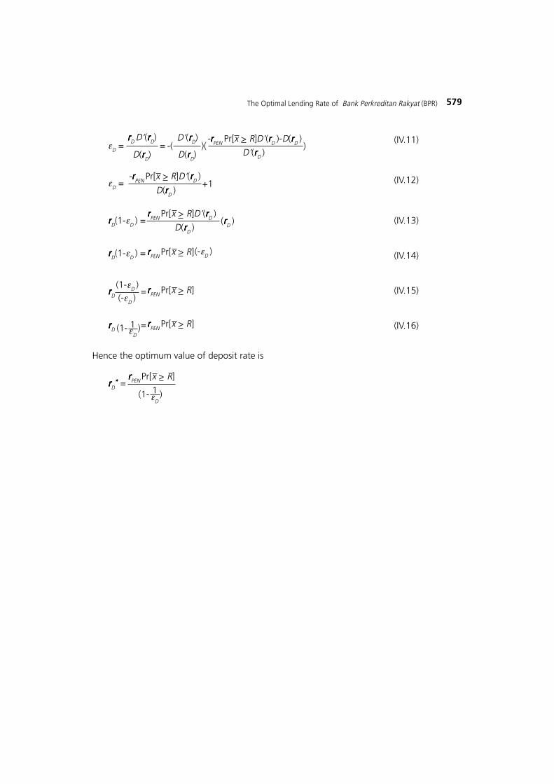
(IV.11)

(IV.12)

(IV.13)

(IV.14)

(IV.15)

(IV.16)

Hence the optimum value of deposit rate is

εD = =rrrrrD D»(rrrrrD)

D(rrrrrD)-( )(

D»(rrrrrD)

D(rrrrrD)

-rrrrrPEN Pr[x > R]D»(rrrrrD )-D(rrrrrD )

D»(rrrrrD ))

εD =-rrrrrPEN Pr[x > R]D»(rrrrrD )

D(rrrrrD )+1

rrrrrD(1-εD ) =rrrrrPEN Pr[x > R]D»(rrrrrD )

D(rrrrrD )(rrrrrD )

rrrrrD(1-εD ) = rrrrrPEN Pr[x > R](-εD )

rrrrrD =rrrrrPEN Pr[x > R](-εD )(1-εD )

rrrrrD =rrrrrPEN Pr[x > R](1- )εD

1

rrrrrD***** =

rrrrrPEN Pr[x > R]

(1- )1εD


APPENDIX 2

JABOTABEK

2SLS-JBTB2SLS-JBTB2SLS-JBTB2SLS-JBTB2SLS-JBTBASSIGN @ALL F

WACF = 0.017485 + 0.017485 * LOG(ALLDEPOSIT) + 0.017485 * PRORISKLIQUI √ 0.450501 *NGANGGUR √ 0.024334 * [SBRIDP/SBTAB] √ 1.4269e-07 * PEGAWAI

SBKRE = 0.32589 √ 0.201178 * LOG[TKRED/TOTAS] + 0.325896 * NPL + 1.204366 * WACF √0.03517 * [SBRIKR/SBTAB] √ 3.119985 * [PDKOKAP/IKK]

System: AA2SLSOKBGS4=2SLS-JBTBEstimation Method: Two-Stage Least SquaresDate: 10/16/04 Time: 15:09Sample: 2 294Included observations: 127Total system (balanced) observations 254Instruments: BOGOR BEKASI KRWANG CLGON TNGR MAKAN

PKAPKO PESTA GRDEF C DEF MIKOT MIDES DAGANGDPEGAWAI TOTKERJA LIBURHAWAN PDDK

Coefficient Std. Error t-Statistic Prob.

C(2) 0.017485 0.000965 18.12797 0.0000C(3) -0.450501 0.071921 -6.263852 0.0000C(5) -0.024334 0.004889 -4.977498 0.0000C(4) -1.43E-07 4.92E-08 -2.902286 0.0040

C(10) 0.325896 0.080782 4.034283 0.0001C(11) -0.201178 0.080604 -2.495893 0.0132C(12) 1.204366 0.442680 2.720625 0.0070C(13) -0.035170 0.015825 -2.222458 0.0272C(14) -3.119985 1.732255 -1.801112 0.0729

Determinant residual covariance 4.49E-05

Equation: ((WACF))=(C(2)+C(2)*LOG(ALLDEPOSIT)+C(2)*(PRORISKLIQUI)+C(3)*(LIBUR)+C(5)*SBRIDP/SBTAB+C(4)*PEGAWAI)

Observations: 127R-squared 0.400364 Mean dependent var 0.141551Adjusted R-squared 0.385739 S.D. dependent var 0.057139S.E. of regression 0.044783 Sum squared resid 0.246676Durbin-Watson stat 1.216792

Equation: ((SBKRE))=(C(10)+C(11)*LOG(TKRED/TOTAS)+C(10)*(NPL)+C(12)*(WACF)+C(13)*SBRIKR/SBTAB+C(14)*(PDKOKAP/IKK))



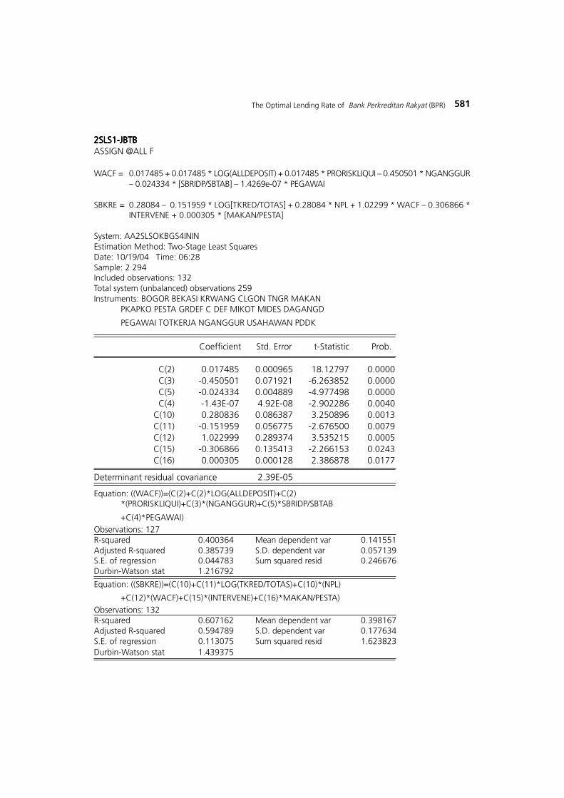
2SLS1-JBTB2SLS1-JBTB2SLS1-JBTB2SLS1-JBTB2SLS1-JBTBASSIGN @ALL F

WACF = 0.017485 + 0.017485 * LOG(ALLDEPOSIT) + 0.017485 * PRORISKLIQUI √ 0.450501 * NGANGGUR√ 0.024334 * [SBRIDP/SBTAB] √ 1.4269e-07 * PEGAWAI

SBKRE = 0.28084 √ 0.151959 * LOG[TKRED/TOTAS] + 0.28084 * NPL + 1.02299 * WACF √ 0.306866 *INTERVENE + 0.000305 * [MAKAN/PESTA]

System: AA2SLSOKBGS4ININEstimation Method: Two-Stage Least SquaresDate: 10/19/04 Time: 06:28Sample: 2 294Included observations: 132Total system (unbalanced) observations 259Instruments: BOGOR BEKASI KRWANG CLGON TNGR MAKAN

PKAPKO PESTA GRDEF C DEF MIKOT MIDES DAGANGD

PEGAWAI TOTKERJA NGANGGUR USAHAWAN PDDK


C(2) 0.017485 0.000965 18.12797 0.0000C(3) -0.450501 0.071921 -6.263852 0.0000C(5) -0.024334 0.004889 -4.977498 0.0000C(4) -1.43E-07 4.92E-08 -2.902286 0.0040

C(10) 0.280836 0.086387 3.250896 0.0013C(11) -0.151959 0.056775 -2.676500 0.0079C(12) 1.022999 0.289374 3.535215 0.0005C(15) -0.306866 0.135413 -2.266153 0.0243C(16) 0.000305 0.000128 2.386878 0.0177


Equation: ((WACF))=(C(2)+C(2)*LOG(ALLDEPOSIT)+C(2)*(PRORISKLIQUI)+C(3)*(NGANGGUR)+C(5)*SBRIDP/SBTAB

+C(4)*PEGAWAI)Observations: 127R-squared 0.400364 Mean dependent var 0.141551Adjusted R-squared 0.385739 S.D. dependent var 0.057139S.E. of regression 0.044783 Sum squared resid 0.246676Durbin-Watson stat 1.216792

Equation: ((SBKRE))=(C(10)+C(11)*LOG(TKRED/TOTAS)+C(10)*(NPL)

+C(12)*(WACF)+C(15)*(INTERVENE)+C(16)*MAKAN/PESTA)Observations: 132R-squared 0.607162 Mean dependent var 0.398167Adjusted R-squared 0.594789 S.D. dependent var 0.177634S.E. of regression 0.113075 Sum squared resid 1.623823Durbin-Watson stat 1.439375


KBI

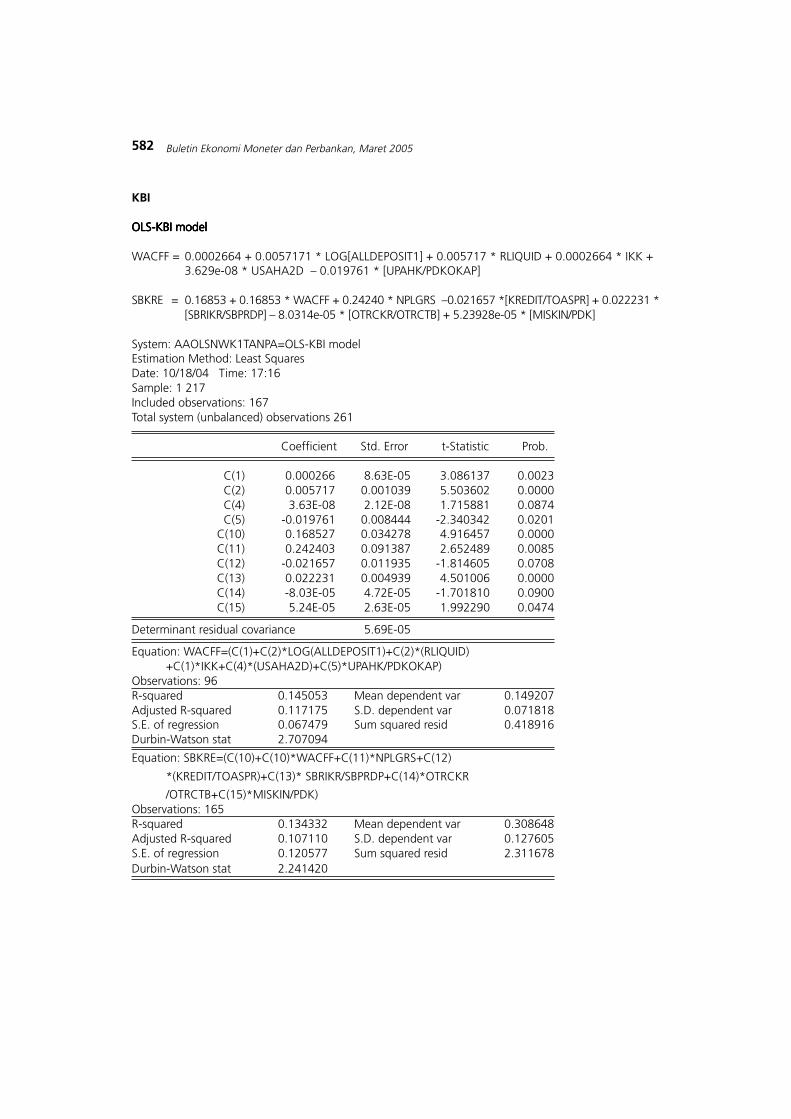
OLS-KBI modelOLS-KBI modelOLS-KBI modelOLS-KBI modelOLS-KBI model

WACFF = 0.0002664 + 0.0057171 * LOG[ALLDEPOSIT1] + 0.005717 * RLIQUID + 0.0002664 * IKK +3.629e-08 * USAHA2D √ 0.019761 * [UPAHK/PDKOKAP]

SBKRE = 0.16853 + 0.16853 * WACFF + 0.24240 * NPLGRS √0.021657 *[KREDIT/TOASPR] + 0.022231 *[SBRIKR/SBPRDP] √ 8.0314e-05 * [OTRCKR/OTRCTB] + 5.23928e-05 * [MISKIN/PDK]

System: AAOLSNWK1TANPA=OLS-KBI modelEstimation Method: Least SquaresDate: 10/18/04 Time: 17:16Sample: 1 217Included observations: 167Total system (unbalanced) observations 261


C(1) 0.000266 8.63E-05 3.086137 0.0023C(2) 0.005717 0.001039 5.503602 0.0000C(4) 3.63E-08 2.12E-08 1.715881 0.0874C(5) -0.019761 0.008444 -2.340342 0.0201

C(10) 0.168527 0.034278 4.916457 0.0000C(11) 0.242403 0.091387 2.652489 0.0085C(12) -0.021657 0.011935 -1.814605 0.0708C(13) 0.022231 0.004939 4.501006 0.0000C(14) -8.03E-05 4.72E-05 -1.701810 0.0900C(15) 5.24E-05 2.63E-05 1.992290 0.0474


Equation: WACFF=(C(1)+C(2)*LOG(ALLDEPOSIT1)+C(2)*(RLIQUID)+C(1)*IKK+C(4)*(USAHA2D)+C(5)*UPAHK/PDKOKAP)


Equation: SBKRE=(C(10)+C(10)*WACFF+C(11)*NPLGRS+C(12)

*(KREDIT/TOASPR)+C(13)* SBRIKR/SBPRDP+C(14)*OTRCKR

/OTRCTB+C(15)*MISKIN/PDK)Observations: 165R-squared 0.134332 Mean dependent var 0.308648Adjusted R-squared 0.107110 S.D. dependent var 0.127605S.E. of regression 0.120577 Sum squared resid 2.311678Durbin-Watson stat 2.241420


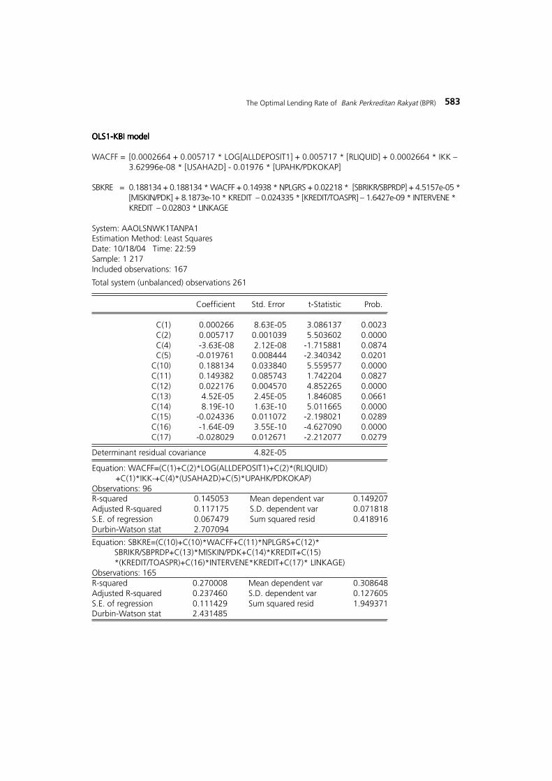
OLS1-KBI modelOLS1-KBI modelOLS1-KBI modelOLS1-KBI modelOLS1-KBI model

WACFF = [0.0002664 + 0.005717 * LOG[ALLDEPOSIT1] + 0.005717 * [RLIQUID] + 0.0002664 * IKK √3.62996e-08 * [USAHA2D] - 0.01976 * [UPAHK/PDKOKAP]

SBKRE = 0.188134 + 0.188134 * WACFF + 0.14938 * NPLGRS + 0.02218 * [SBRIKR/SBPRDP] + 4.5157e-05 *[MISKIN/PDK] + 8.1873e-10 * KREDIT √ 0.024335 * [KREDIT/TOASPR] √ 1.6427e-09 * INTERVENE *KREDIT √ 0.02803 * LINKAGE

System: AAOLSNWK1TANPA1Estimation Method: Least SquaresDate: 10/18/04 Time: 22:59Sample: 1 217Included observations: 167

Total system (unbalanced) observations 261


C(1) 0.000266 8.63E-05 3.086137 0.0023C(2) 0.005717 0.001039 5.503602 0.0000C(4) -3.63E-08 2.12E-08 -1.715881 0.0874C(5) -0.019761 0.008444 -2.340342 0.0201

C(10) 0.188134 0.033840 5.559577 0.0000C(11) 0.149382 0.085743 1.742204 0.0827C(12) 0.022176 0.004570 4.852265 0.0000C(13) 4.52E-05 2.45E-05 1.846085 0.0661C(14) 8.19E-10 1.63E-10 5.011665 0.0000C(15) -0.024336 0.011072 -2.198021 0.0289C(16) -1.64E-09 3.55E-10 -4.627090 0.0000C(17) -0.028029 0.012671 -2.212077 0.0279


Equation: WACFF=(C(1)+C(2)*LOG(ALLDEPOSIT1)+C(2)*(RLIQUID)+C(1)*IKK-+C(4)*(USAHA2D)+C(5)*UPAHK/PDKOKAP)


Equation: SBKRE=(C(10)+C(10)*WACFF+C(11)*NPLGRS+C(12)*SBRIKR/SBPRDP+C(13)*MISKIN/PDK+C(14)*KREDIT+C(15)*(KREDIT/TOASPR)+C(16)*INTERVENE*KREDIT+C(17)* LINKAGE)


the optimal lending rate of bank perkreditan … · the optimal deposit and lending rate, ... nbl...

Documents