1

The New (Version 4) Calibration of the Nighttime 532nm Channel of the CALIPSO Lidar*

5

J. Kar 1,2, M. A. Vaughan2, K. P. Lee1,2, J. Tackett1,2 , M. Avery2, A. Garnier1, B. Getzewich1,2,

W. Hunt1,2,**, D. Josset1,2, Z. Liu2, P. Lucker1,2, B. Magill1,2, A. Omar2, R. Rogers2, T. Toth2,

C. Trepte2, J-P. Vernier1,2, D. Winker2, S. Young3

10

1Science Systems and Applications Inc., Hampton, VA, USA

15 2NASA Langley Research Center, Hampton, VA, USA

3CSIRO Oceans & Atmosphere Flagship, Aspendale, VIC, Australia

**Deceased 20

*This paper is dedicated to the memory of W. Hunt.

Abstract. 25

The data products from the Cloud-Aerosol Lidar with Orthogonal Polarization (CALIOP) on board

Cloud-Aerosol Lidar and Infrared Pathfinder Satellite Observations (CALIPSO) were recently

updated following the implementation of a new (version 4.1) calibration algorithm for all the level

1 products. We present the motivation for and the implementation of the version 4.1 nighttime 532 30

nm parallel channel measurements. This is the most fundamental calibration of CALIOP data since

all other measurements, i.e the 532 nm nighttime perpendicular, daytime 532 nm as well as 1064

nm are tied to this calibration. The new calibration is shown to resolve the discrepancies in the

earlier version and also leads to an improved representation of the stratospheric aerosols. Initial

validation results using ground based and airborne lidar measurements are also presented. 35

2

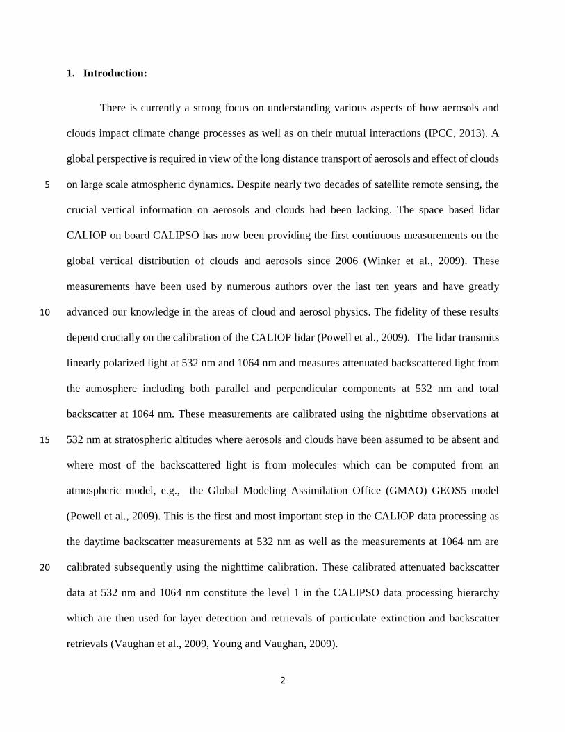
1. Introduction:

There is currently a strong focus on understanding various aspects of how aerosols and

clouds impact climate change processes as well as on their mutual interactions (IPCC, 2013). A

global perspective is required in view of the long distance transport of aerosols and effect of clouds

on large scale atmospheric dynamics. Despite nearly two decades of satellite remote sensing, the 5

crucial vertical information on aerosols and clouds had been lacking. The space based lidar

CALIOP on board CALIPSO has now been providing the first continuous measurements on the

global vertical distribution of clouds and aerosols since 2006 (Winker et al., 2009). These

measurements have been used by numerous authors over the last ten years and have greatly

advanced our knowledge in the areas of cloud and aerosol physics. The fidelity of these results 10

depend crucially on the calibration of the CALIOP lidar (Powell et al., 2009). The lidar transmits

linearly polarized light at 532 nm and 1064 nm and measures attenuated backscattered light from

the atmosphere including both parallel and perpendicular components at 532 nm and total

backscatter at 1064 nm. These measurements are calibrated using the nighttime observations at

532 nm at stratospheric altitudes where aerosols and clouds have been assumed to be absent and 15

where most of the backscattered light is from molecules which can be computed from an

atmospheric model, e.g., the Global Modeling Assimilation Office (GMAO) GEOS5 model

(Powell et al., 2009). This is the first and most important step in the CALIOP data processing as

the daytime backscatter measurements at 532 nm as well as the measurements at 1064 nm are

calibrated subsequently using the nighttime calibration. These calibrated attenuated backscatter 20

data at 532 nm and 1064 nm constitute the level 1 in the CALIPSO data processing hierarchy

which are then used for layer detection and retrievals of particulate extinction and backscatter

retrievals (Vaughan et al., 2009, Young and Vaughan, 2009).

3

The molecular normalization was originally implemented between 30 and 34 km and

remained unchanged in the subsequent versions of CALIPSO data up to version 3.30 (Powell et

al., 2009). In recent years it has become clear that this region is not completely free of aerosols

and thus the calibration needed to be improved (Vernier et al., 2009, Powell et al., 2009). In this

paper we report the results of a new calibration algorithm for the nighttime 532 nm data which has 5

been implemented for the new version 4.10 (V4) of CALIOP data and which was released in April

2014. In this new algorithm, the molecular normalization is now applied at 36-39 km where

particulates are nearly absent. However, this altitude regime is near the limit of CALIOP detection

range and thus has the attendant problem of significantly lower signal to noise ratio (SNR)

necessitating more averaging of the data. Further an improved meteorological data set from 10

MERRA 2 reanalyses is employed in the new version of the data. In this paper, we present the

details of this new calibration as well as improvements in the new version as a result of these

changes.

2. Motivation and implementation of the new (V4) calibration for nighttime 532 nm data

2.1 The need for a new calibration 15

The initial decision to calibrate the CALIOP nighttime 532 nm channel signals at 30-34 km was

dictated by the need to have sufficient molecular backscatter to provide a robust SNR ( required

to be at least 50 averaged over 5 km vertically and 1500 km horizontally) as well as low or

negligible contamination from stratospheric aerosol loading (Hunt et al., 2009). Vernier et al.

(2009) analyzed the time sequence of attenuated scattering ratios (ratio of total attenuated 20

backscatter and the molecular backscatter, SR) calculated from CALIOP 532 nm measurements

over the tropics and showed anomalously low values (SR<1) above 34 km as well as in the lower

4

stratosphere. Since molecular normalization at 30-34 km implies SR should be one at these

altitudes, this indicated an inadequate calibration in the CALIOP data. They adjusted the

calibration by normalizing the SR values by calculated SR at 36-39 km. Figure 1 (reproduced

from Vernier et al. (2009)) shows the latitude time cross section of the adjusted calibration constant

which effectively represents the revised aerosol SR at 30-34 km. As can be seen only minor 5

adjustment is required in the mid latitudes, but there is ~ 2-12% underestimation in SR at 30-34

km in the tropics.

Figure 1. Zonally averaged time-latitude cross section of the adjusted calibration

coefficient obtained using the CALIOP version 2 data (reproduced from Vernier et al., 10

2009).

A similar problem was noted by Powell et al. (2009) when they found a persistent dip in the tropics

in clear air SR ( < 1) between 8-12 km, which also underscored the need for an improvement in

calibration.

5

The most extensive and accurate measurements of stratospheric aerosols have come from

the Stratospheric Aerosol and Gas Experiment II (SAGE II) instrument. SAGE II has provided the

extinction coefficient profiles in the stratosphere using solar occultation technique from 1984

through 2005 (Mauldin et al., 1985, Thomason et al., 1997, Damadeo et al., 2013). Between 1991-

1996 the stratosphere was loaded with volcanic aerosols from Pinatubo eruption and no meaningful 5

data are available for that period. However, the stratospheric aerosol loading has remained near

the background levels since 1998 except for some modulation by smaller volcanoes (Vernier et

al., 2011).

10

Figure 2. Scattering ratios estimated from the extinctions retrieved from SAGE II at 30-34

km (solid lines) and at 36-39 km (dashed lines).

6

Figure 2 shows the zonal average of SR at 30-34 km (solid lines) and 36-39 km (dashed lines) as

derived from the SAGE II extinction retrievals between 1998 and 2005 using the latest version 7.0

of SAGE II data (Damadeo et al., 2013). The aerosol extinctions at 525 nm from SAGE II have

been converted to scattering ratios using a stratospheric aerosol lidar ratio of 50 sr; an Angstrom

exponent of 1.6 was then used to convert the data from 525 nm to 532 nm (Khaykin et al., 2017). 5

All the extinction data with estimated error less than 100% were included from both sunset and

sunrise occultations. The data before 1998 were not used to avoid the contamination from the

Pinatubo volcano. As can be seen, the SR for the background aerosols can reach as much as 7-8%

at 30-34 km over the tropical latitudes while decreasing steeply to ~2% at the polar regions.

Further, significant seasonal variation at these altitudes can also be seen with maximum extinction 10

being in winter and lowest in summer. On the other hand at 36-39 km, the SR values are by and

large uniform over all latitudes at about 2%, with very little seasonal variability. This result again

suggests that there is a low bias in the CALIOP data in the V3 calibration algorithm and indicates

that a better calibration with minimal aerosol contamination is needed. With more data acquisition

and improved understanding of the quality of the data, it was realized that the calibration altitude 15

can be raised to 36-39 km.

2.2 CALIOP 532 nm nighttime calibration method

The primary CALIOP nighttime 532 nm calibration algorithm uses the parallel channel

measurements of the geolocated, range scaled and energy and gain-normalized signals (X) and is

defined simply by the equation: 20

C = 𝑋(𝑍𝑐 )

𝛽(𝑍𝑐) 𝑇2(𝑍𝑐) (1)

7

with X (z) = 𝑟2 𝑆(𝑧)

𝐸0 𝐺𝐴 , (2)

S being the measured signal after subtracting the solar background and digitizer offset

voltages, Zc is the calibration altitude, E0 the laser energy, Ga is the amplifier gain, β is the parallel

backscatter coefficient from molecules and aerosols and T2 is the two-way transmission:

T2 (z) = exp {−2 ∫ 𝜎 [𝑧(𝑟′)] 𝑑𝑟′𝑟

0} (3) 5

Where σ is the volume extinction coefficient and is the sum of molecular scattering, aerosol

scattering and ozone absorption coefficients. The latter are computed from a molecular model and

accurate calibration of CALIOP nighttime 532 nm data depends crucially upon this model. In the

past versions up until V4.0, CALIOP calibration algorithm had used the molecular and ozone

number densities from the NASA GMAO models. These model parameters keep getting updated 10

with improvements in the inputs and the assimilation system and successive versions of GMAO

models were used for different versions of CALIOP data. For V4.10 the latest Modern Era

Retrospective Analysis for Research and Applications version 2 (MERRA 2) model from GMAO

has been adopted (Molod et al., 2015). Apart from the general improvements, MERRA 2 for the

first time assimilates aerosol information from various satellite and ground based measurements 15

and the aerosol radiative feedback to the atmospheric fields. The estimation of the 532 nm parallel

channel calibration co-efficient is carried out using equation (1) assuming that there is no aerosol

in the calibration region. Even with this assumption, the calibration procedure involves significant

filtering and averaging of the measured signals. These are briefly described in the following

sections. 20

8

2.3 The new spike filter

As described in Powell et al. (2009), the lidar signal profiles are carefully filtered in a three-

step process in order to eliminate the large noise spikes often encountered in the calibration region

before using them in the subsequent averaging scheme leading to the computation of the

calibration coefficient. These large noise spikes occur particularly over an extended area over the 5

continent of South America and adjoining South Atlantic Ocean and is known as the South Atlantic

Anomaly (SAA) where high energy charged particles from the Sun and cosmic rays trapped in the

Van Allen belts come down to low altitudes and affect the CALIOP sensor leading to the noise

spikes. In the first step, an adaptive spike filter is used to remove the outliers from the 11 signal

profiles (X) of 5 km horizontal resolution occurring inside each calibration sample region (55 km 10

horizontally for both versions and 30-34 km in V3 and 36-39 km in V4 in the vertical direction)

beyond a low and high threshold. The thresholds are determined by the expected molecular signal

and the uncertainties from the random noise in the measurement process (Powell et al., 2009). In

order to take care of the generally lower signals at the raised calibration altitudes in the new V4

scheme, the low and high threshold values of this uncertainty were adjusted so as to eliminate not 15

more than about 0.15% of the data at both ends.

The valid data segments from the first step are further filtered for large excursions of signal

values in the second step of data filtering by estimating the noise to signal ratio (NSR). The NSR

is defined as the ratio of the standard deviation and the mean value of all the valid signals and the

calculated NSR is compared against an empirical threshold value. If the NSR value estimated from 20

the valid signal profiles is less than the threshold, then the mean profile from the valid signals is

constructed (“calibration-ready”). For V4, this step necessitated some careful consideration, since

retaining the NSR threshold values used in the V3 tended to preferentially take out the low signal

9

with high noise (high NSR) data at 36-39 km region thus leading to unrealistically high calibration

coefficients. Figure 3 shows the NSR thresholds (median + 5 median absolute distance) used in

V4 as a function of the granule elapsed time (function of latitude). They also vary from month to

month to take care of seasonal variation in the noise background. An objective criterion was used

to choose these values which minimize the difference in mean calibration coefficients over the 5

SAA region and the non-SAA region within the same latitude band.

Figure 3. The NSR thresholds employed in V4 algorithm for various months as a function

of granule elapsed time. 10

In the third step, the adaptive filter is once again applied but to the mean of the “calibration-

ready” profile. If the latter passes this test, then it is used for calculation of the calibration

coefficient using equation (1) for the 55 km calibration sample region ( the minimum horizontal

distance over which CALIOP collects data uniformly from all the three instruments onboard

CALIPSO is called a Payload Data Acquisition Cycle, PDAC and is equal to 55 km). The basic 15

10

calibration algorithm over a single PDAC with the new spike filter as mentioned above is similar

in both V3 and V4. Further details with examples of the actual filtering and the mathematical basis

for computation of the calibration coefficient are available in Powell et al. (2009).

An estimate of the efficiency of the new calibration algorithm may be obtained from the

calibration success rate, which is just the ratio of the number of successful calibrations and the 5

attempted calibrations within a specified area.

Figure 4. Spatial distribution of the calibration success rates for V3 and V4 for the month

of July 2010. The data are binned in 2ox2o in latitude and longitude.

Figure 4 shows the mean calibration success rate in percentage of the attempted calibration for the 10

month of July 2010 for V3 and V4. Both the versions have broadly similar calibration success rates

over the globe, with somewhat more noise in V4, as may be expected. Over most of the globe, the

success rate is over 90% in both versions. However significantly lower success rates (in blue)

occur over the SAA region mentioned above. This is the region where the adaptive filter removes

a significant number of calibration profiles leading to the lower success rates. The success rate 15

11

also falls significantly over Antarctica and its vicinity with the V4 calibration success rate being

somewhat lower than in V3, once again indicating the harsh radiation environment over this area,

which affects the SNR particularly at higher altitudes (Hunt et al., 2009).

2.4 The new averaging scheme

The calibration coefficients obtained over individual PDACs as described above are further 5

smoothed along the orbital track to remove noise. In V3 this smoothing was done over 27 PDACs

by computing running averages, covering a distance of 1485 km and leading to the final calibration

coefficients for the 532 nm parallel channel. While raising the molecular normalization region to

36-39 km in V4 will clearly lead to better calibration in terms of significant reduction of aerosol

contamination, we have to now deal with a significantly reduced SNR because of reduced 10

molecular density. The SNR from CALIOP measurements has been simulated using the FREESIM

simulation package (Hunt, 2012, NASA Langley internal report). In the V3 calibration algorithm

(30-34 km), the smoothing of the calibration coefficients over 27 PDACs (1485 km) resulted in a

simulated SNR of 57.1 for the molecular backscatter signals. If the same level of smoothing were

to be retained in the new calibration region of 36-39 km, then the simulated SNR drops 15

significantly to 32.1.

12

Figure 5. 12 SNR profiles from CALIOP measurements representing various latitudes and

seasons. The thick red line is the mean profile.

This sharp drop in simulated SNR is consistent with the measured SNR profiles as can be

seen in Figure 5, where we have shown 12 measured SNR profiles from CALIOP representing

the different seasons and a large range of latitudes over 2009-2012. The values were normalized 5

to the value at 32 km. In order to recover the same level of SNR as V3, the simulations indicate

that the data has to be smoothed over at least 4710 km or 86 PDACs. An examination of the

calibration coefficients from consecutive orbits showed no significant variability from day to day

indicating that no loss of accuracy will occur by taking average over multiple orbits. On the other

hand it would be desirable to reduce averaging distance over the same orbit. Therefore it was 10

decided to average the calibration coefficients over 11 consecutive orbits with 11 PDACs from

each orbit (605 km along track over each orbit) for the new calibration (i.e. 121 PDACs in all

covering a distance of 6655 km).

3. Assessment of CALIOP V4 calibration

With these revisions in the averaging scheme and the spike filter, the calibration of the parallel 15

channel nighttime 532 nm measurements was carried out for V4.

13

Figure 6. The time series of the V4 532 nm CALIOP nighttime parallel calibration

coefficient. The values have been normalized by the initial value (6.1483 x1010). The letters

represent the various instrument events that affect the calibration: (B) -- boresight

alignment, (E) – etalon temperature adjustment, (L) – laser switch.

Figure 6 shows the time series of the V4 calibration coefficient over the entire mission period 5

from 2006 through 2016. The granule average values of the coefficients (in blue) have been

smoothed over 10 granules (in thick black). Over short term, the sharp upward revisions in

calibration mostly correspond to the boresight alignment and etalon scan procedures. These

procedures take place periodically. Apart from these, there were two significant one-time events

that took place. Firstly, the primary laser started showing signs of degradation and was replaced 10

by the second laser in March 2009. Secondly, the laser pointing angle was changed from 0.3 degree

to 3.0 degree in November 2007. The longer term downward trends in the calibration coefficient

values likely represent component degradation (as may have occurred during the operation of the

first laser), boresight misalignment and etalon mismatch (Hunt et al., 2009).

3.1. Overall differences between V3 and V4 calibration 15

14

Figure 7. a) The fractional change from V3 to V4 in the zonally averaged 532 nm

calibration coefficient for 4 months in 2010 (left panel) and b) the corresponding zonally

averaged relative uncertainty in the calibration coefficient for the same months (right

panel).

Figure 7a shows the zonal mean distribution of the fractional change in the 532 nm nighttime 5

calibration coefficient from V3 to V4 for the months of January, April, July and October 2010

representing the four seasons. The calibration coefficient in V4 obtained from measurements at

36-39 km decreases by 2-3% on average as compared to the calibration coefficients derived at 30-

34 km in V3 as may be expected because of negligibly low aerosol contamination at 36-39 km as

shown in Figure 2. There is some seasonal variation in the amount of change from V3 to V4 most 10

notably at the southern tropics. Seasonal and inter annual variations in the calibration change may

be expected as the aerosol loading at 30-34 km responds to the stratospheric dynamics. One

important criterion for improving the calibration in V4 was to retain the same level of the estimated

relative random uncertainty in the calibration coefficient. Figure 7b shows the zonal mean relative

uncertainty in the calibration coefficient in V3 and V4 for the four months corresponding to Figure 15

7a. Overall the random uncertainty is less than 2-3% with higher values over the SAA region and

near the poles because of the noise in the measurements in these regions. This is of the same order

of uncertainty as in V3.

15

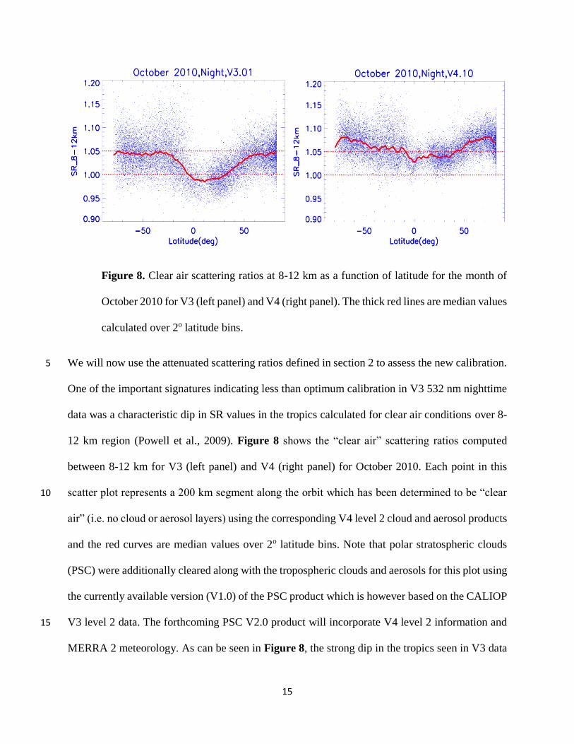
Figure 8. Clear air scattering ratios at 8-12 km as a function of latitude for the month of

October 2010 for V3 (left panel) and V4 (right panel). The thick red lines are median values

calculated over 2o latitude bins.

We will now use the attenuated scattering ratios defined in section 2 to assess the new calibration. 5

One of the important signatures indicating less than optimum calibration in V3 532 nm nighttime

data was a characteristic dip in SR values in the tropics calculated for clear air conditions over 8-

12 km region (Powell et al., 2009). Figure 8 shows the “clear air” scattering ratios computed

between 8-12 km for V3 (left panel) and V4 (right panel) for October 2010. Each point in this

scatter plot represents a 200 km segment along the orbit which has been determined to be “clear 10

air” (i.e. no cloud or aerosol layers) using the corresponding V4 level 2 cloud and aerosol products

and the red curves are median values over 2o latitude bins. Note that polar stratospheric clouds

(PSC) were additionally cleared along with the tropospheric clouds and aerosols for this plot using

the currently available version (V1.0) of the PSC product which is however based on the CALIOP

V3 level 2 data. The forthcoming PSC V2.0 product will incorporate V4 level 2 information and 15

MERRA 2 meteorology. As can be seen in Figure 8, the strong dip in the tropics seen in V3 data

16

no longer appears in V4 with relatively very few points showing SR < 1. This along with the

general meridional uniformity of “clear air” SR indicates a significantly improved calibration in

V4 of CALIOP data. It should be noted that there may be tenuous particulate loading in the 8-12

km region which might be below the layer detection threshold of CALIOP, which will nonetheless

show up in scattering ratios with SR values in excess of the expected clear air SRs (~1). 5

Figure 9. Zonally and vertically (over 30-34 km) averaged SR calculated from V4

CALIOP attenuated backscatter data for January, April, July and October 2009. Data over

SAA region were not included and are binned over 2o in latitude (with at least 50 points

within the latitude bin). 10

17

The old calibration altitude range of 30-34 km presents a useful region for calibration assessment

in the new version, since SR was essentially forced to 1 in this region in V3 and should be different

in V4. Figure 9 shows the zonal mean distribution of SR averaged over 30-34 km as estimated

from the level 1B files from V4 for January, April, July and October 2009 representing the four

seasons. The SR values at 30-34 km in V4 varies between ~3%-10% in all the cases with 5

significant seasonal variations while in V3 these values were all forced to one.

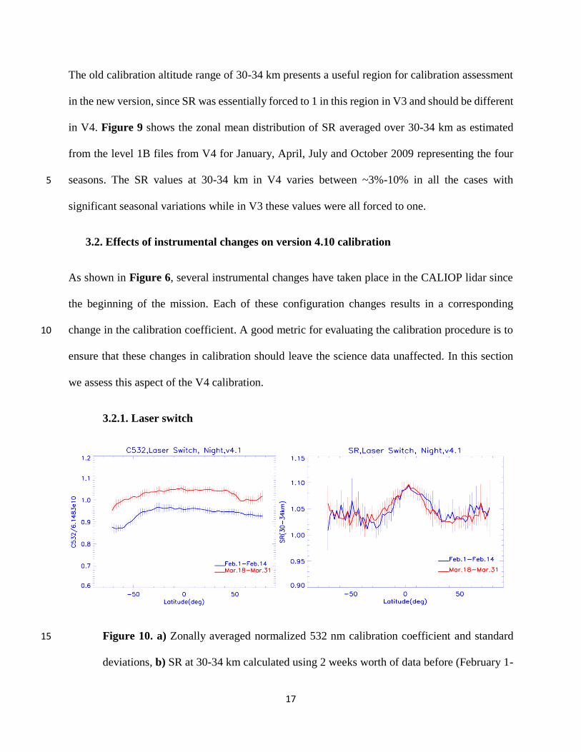
3.2. Effects of instrumental changes on version 4.10 calibration

As shown in Figure 6, several instrumental changes have taken place in the CALIOP lidar since

the beginning of the mission. Each of these configuration changes results in a corresponding

change in the calibration coefficient. A good metric for evaluating the calibration procedure is to 10

ensure that these changes in calibration should leave the science data unaffected. In this section

we assess this aspect of the V4 calibration.

3.2.1. Laser switch

Figure 10. a) Zonally averaged normalized 532 nm calibration coefficient and standard 15

deviations, b) SR at 30-34 km calculated using 2 weeks worth of data before (February 1-

18

14, 2009) and after (March 18-31,2009) the laser switch. SR profiles were calculated over

2o latitude intervals from each granule and then averaged over all granules for the latitude

bin (with a minimum number of 50 SR profiles in each bin). Data over SAA were not

included.

There are two lasers onboard CALIPSO and the CALIOP data production in June 2006 was started 5

with the primary laser (called laser 2). However the canister housing the optics and the high voltage

components gradually lost pressure from a leak and the laser started showing anomalous behavior

presumably resulting from coronal discharge at low pressures. As a result, the primary laser was

turned off on February 16, 2009 and the backup laser (called laser 1) was subsequently activated

on March 12, 2009 which has since been continuously operating. This is the largest configuration 10

change so far in the mission and led to a very large concomitant change in the calibration

coefficients as can be seen in Figure 10 which shows (left panel) the zonal mean calibration

coefficients for two periods representing pre-switch (February 1-14) and post-switch (March 18-

31) periods. However the zonal mean SR values (right panel) computed for these two periods agree

quite well and clearly indicates that the calibration algorithm has been correctly implemented. 15

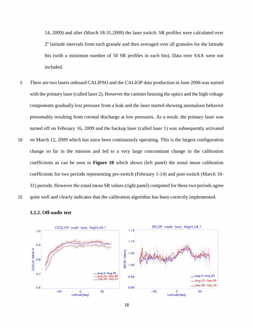
3.2.2. Off-nadir test

19

Figure 11. Same as in Figure 10 using data before (August 4-20, 2007), during

(August 22-September 6, 2007) and after (September 8-24, 2007) the off-nadir laser

pointing test.

Another significant instrument event took place in November 2007 when the pointing angle of the

laser was changed from 0.3 degree to 3.0 degree in order to avoid the effects of specular reflections 5

(Hunt et al., 2009). An advanced test of this change was carried out between August 22 and

September 6, 2007 when the pointing angle was held at 3 degree and changed back to 0.3 degree

pending final change in November 2007. Figure 11a (left panel) shows the normalized calibration

coefficients before the test (August 4 - August 20, 2007), during the test (August 22 – September

6, 2007) and after the test (September 8 – September 24, 2007). Although not as large as the change 10

from the laser switch, significant changes in the calibration coefficients can still be discerned

among the curves. Note that the calibration coefficients do not exactly revert back to the pre-test

values and are significantly lower. This is because this test took place when the primary laser was

still operational and the calibration coefficient was continuously decreasing during this period.

However despite this, the zonal mean SR values (right panel) at 30-34 km are all essentially 15

coincident thus testifying to the robustness of the calibration algorithm.

3.2.3. Boresight alignment

The alignment between the CALIOP transmitter and the receiver is maintained by a

boresight alignment mechanism that adjusts the laser pointing direction to maximize the return

signal and is carried out occasionally. A large boresight alignment took place on December 7, 20

2009. Figure 12 shows zonally averaged calibration coefficients before (November 21- December

6, 2009) and after (December 8 – December 23, 2009) the boresight alignment. The calibration

coefficients changed significantly in response to the event. However as can be seen in the right

20

panel below, the scattering ratio didn’t change significantly before and after the events once again

indicating a proper implementation of the new calibration algorithm.

Figure 12. Same as in Figure 10 using data a) before (November 21-December 6, 2009) 5

and b) after (December 8-23, 2009) the boresight alignment procedure on December 7,

2009.

3.3 Impacts on science: stratospheric aerosol

As shown above, the new calibration coefficients in V4 leads to a generally upward revision of the

level 1 attenuated backscatter coefficients by 3-6% depending upon the location and season. In 10

particular, Figure 9 shows that variations in aerosol loading at the stratospheric altitudes may be

robustly captured in the new data. This is illustrated further in Figure 13, which shows the zonally

averaged height latitude cross sections of SR in November 2007 and May 2009 for both V3 and

V4.

21

Figure 13. Height latitude cross sections of the attenuated scattering ratio calculated using

V3 and V4 level 1 data for November 2007 (top two panels) and for May 2009 (bottom

two panels).

In both these months, distinct structures can be observed in the stratospheric regions between 20 5

km and 30 km in the tropics which are likely linked to the quasi-biennial oscillations (QBO) of

lower stratospheric winds between about 20-35 km. In November 2007, dominant westerly shear

prevailed in the stratosphere (monthly mean zonal wind at Singapore at 10 hPa = 18 ms-1 ) leading

to a characteristic double horn structure in the tropical stratospheric aerosol distribution (Trepte

and Hitchman, 1992). In the V3 map (top left) this structure can be seen only partially, while it is 10

much more prominent and clear in the V4 map (top right). On the other hand, dominant easterly

22

shear prevailed in the stratosphere in May 2009 (monthly mean zonal wind at Singapore at 10 hPa

= -34.2 ms-1) during which aerosol lofting is expected to take place in the tropics and lateral

transport is inhibited (Trepte and Hitchman, 1992). The aerosol lofting is not seen in the V3 map

(bottom left), but is quite clearly observed in the V4 map (bottom right). This demonstrates that

the V4 CALIOP data can provide important and robust information in the stratosphere. This is 5

further seen in the time series of SR at 30-34 km from 2006-2016 (Figure 14). A CALIOP

stratospheric aerosol product is currently under development which exploits this improved

calibration.

Figure 14. Scattering ratio at 30-34 km as a function of time and granule elapsed time 10

(function of latitude) for the period June 2006 through 2016. The data has been smoothed

over 10 PDACs.

4.0 Initial validation of the version 4.10 calibration

4.1. Comparison with HSRL

The airborne High Spectral Resolution Lidar (HSRL) developed at NASA Langley Research 15

Center has been used over the years for validation of CALIOP lidar calibration through coincident

underflights (Hair et al., 2008). The HSRL provides internally calibrated attenuated backscatter

23

measurements at 532 nm, thus avoiding the issues about aerosol contamination at calibration

altitudes for space borne lidars and are very accurate, ~1-2% (Rogers et al., 2011).

Table 1. Dates and missions under which HSRL nighttime flights were conducted.

Table 1 lists the different field missions and the dates when the HSRL underflights took place 5

during nighttime between June 2006 and June 2014. Some of these flights were solely for the

purpose of CALIPSO validation activity and some were under the auspices of a more general field

mission with other objectives. A total of 35 nighttime flights were used for comparison with the

coincident CALIOP measurements. For comparison with CALIOP, the total attenuated backscatter

estimated from HSRL for “clear-air” regions are first corrected for the molecular attenuation 10

between the HSRL reference altitude (~1.5 – 2 km below the flight altitude) and the CALIOP

altitude. Difference profiles between HSRL and CALIOP are then calculated using the equation:

ΔC(r) = 𝛽′

𝐻𝑆𝑅𝐿 (𝑟) − 𝛽′

𝐶𝐴𝐿𝐼𝑂𝑃 (𝑟)

𝛽′𝐻𝑆𝑅𝐿

(𝑟) (4)

24

where, 𝛽′𝐻𝑆𝑅𝐿

(𝑟) is the mean of the coincident and cloud-free total attenuated backscatter from

HSRL at range r and referenced to CALIOP altitude, and 𝛽′𝐶𝐴𝐿𝐼𝑂𝑃

(𝑟) is the corresponding mean

of total attenuated backscatter from CALIOP at range r. For further details of the comparison

methodology, the reader is referred to Rogers et al. (2011). A single difference value was estimated

for each HSRL coincident underflight by taking average over the horizontal and vertical 5

dimensions of the clear-air region. Figure 15a shows the histogram of these differences and

essentially represents the assessment of the CALIOP calibration. The distributions are shown for

both V3 and V4. The mean difference between HSRL and CALIOP was 3.6% using V3 calibration,

which has now been reduced significantly to 1.6% in V4, indicating a much improved calibration

for CALIOP V4 algorithm. Most of the flights took place in the northern mid latitudes between 10

30oN-40oN (Figure 15b). Although the comparison covers only a limited latitude range, no

obvious latitude dependence can be discerned. This figure shows the corresponding mean

differences from V3 to V4 for the various flights. Most of differences from the individual flights

have decreased significantly, with the exception of a few outliers.

15

25

Figure 15. a) Distributions of the average differences between HSRL and CALIOP of the

532 nm total attenuated backscatter in the nighttime clear air regions of coincidence and b)

the differences as a function of latitude. V3 data are shown in green while the V4 data are

shown in magenta. N in a) represents the total number of coincidence profiles. The error 5

bars in b) represent the standard error of the mean.

4.2. Comparison with NDACC lidar at Dumont d’Urville

Ground based data from a number of lidars are available through the Network for the Detection of

Atmospheric Composition Change (NDACC). For this initial validation and in view of the noisy

environment over Antarctica and the availability of a large number of comparable backscatter 10

profiles, we have selected to present the comparison between CALIOP and the Lidar for Ozone

and Aerosols for NDACC in Antarctica (LOANA) at Dumont d’Urville, located at the French

Antarctic station (67oS, 140oE). Correlative data from LOANA are available for most of the years

when CALIPSO has been functional thus offering opportunities for a robust comparison. Aerosol

26

and PSC measurements are carried out using this lidar at night between 8 km and 32 km and in

clear sky conditions at 532 nm and 1064 nm, the vertical resolution of the profiles being 60 m

(David et al., 2012). The lidar signals in the parallel channel are averaged over 5 minutes to reduce

the noise level. Scattering ratio profiles are calculated using the Klett method with an uncertainty

in SR between 5-10% from various sources. The molecular densities used in the calculations are 5

obtained from daily radiosonde launches.

For the comparison, we first check each lidar SR profile available from LOANA database.

If the maximum value of the SR profile is less than 1.5, then it is considered to be a “clear air”

profile and is selected for comparison. All CALIOP data falling within a 2ox2o in latitude and

longitude coincidence box is used to select the CALIOP profiles for the same day and year. 10

Subsequently, the CALIOP attenuated backscatter profiles are filtered for cloud and aerosol layers

above 8 km using V4 level 2 data as well as PSCs using V1.0 CALIPSO PSC product. All the

clear air CALIOP profiles from within the coincidence box for a specific day are then averaged

and SR profiles are calculated after rejecting SR values above 1.5, to be consistent with the

LOANA “clear-air” profiles. The CALIOP profiles are then interpolated to the LOANA altitude 15

grid and compared with the LOANA profile for that day (averaged if multiple profiles were

available for a single day) yielding difference profiles:

Δ =100. (𝑆𝑅𝐶𝐴𝐿𝐼𝑂𝑃 − 𝑆𝑅𝐿𝑂𝐴𝑁𝐴)

𝑆𝑅𝐿𝑂𝐴𝑁𝐴 (5)

A total of 94 days worth of data were compared covering all available LOANA measurements

from 2006 to 2014 varying from a minimum of 3 days in 2009 to a maximum of 18 days in 2014. 20

27

Figure 16. Profile of the mean difference in SR from CALIOP and LOANA lidars for

clear air conditions above 8 km. Coincident data from 2007 through 2014 have been used

for this comparison. The red dashed lines demarcate 5% difference.

Figure 16 shows the mean difference profile obtained from this comparison. The agreement 5

between the two instruments is within 5% on average. Given the noise considerations, which are

particularly high at Antarctic latitudes (Hunt et al., 2009) and all the other uncertainties from the

different normalization procedures adopted by the two instruments, this agreement using a large

number of samples confirms the significantly improved calibration of CALIPSO version 4 level 1

data. 10

5.0 Conclusions.

Accurate calibration of the CALIOP nighttime 532 nm measurements is the most important

element in ensuring robustness of the CALIOP data products since all the other measurements

derive their calibration from this. In the V4 algorithm, the calibration altitude for the nighttime

parallel channel has been raised from 30-34 km to 36-39 km which ensures no or minimal 15

28

contamination from stratospheric aerosols for the molecular normalization procedure. We have

presented the salient features of the new calibration procedure and pointed out the improvements

in the V4 data arising from this new calibration. The inconsistencies in the V3 data owing to the

old calibration have now been resolved. The uncertainties in the V4 calibration are of the same

order as in V3 and the calibration correctly adjusts to the periodic instrument changes like 5

boresight alignments, leaving the science data unaffected. The improved calibration also lends

itself to a robust representation of stratospheric aerosols. The initial validation of the calibration

using the coincident HSRL measurements at northern mid latitudes indicates an agreement of <1%

suggesting a robust calibration. Comparison with a ground based lidar at Antarctica also gives

good agreement (within 5%). Overall a significant improvement in CALIOP primary calibration 10

has been achieved in V4 and this should result in a corresponding improvement in the level 2

CALIOP products downstream.

Acknowledgements: The ground based lidar data from Dumont D’Urville were taken from the

NDACC database and the authors are grateful to the instrument team for making the data publicly 15

available. Further, M. Pitts and F. Cairo are acknowledged for advice on the clear-air profiles from

the lidar at Dumont d’Urville. SAGE II as well as the level 1 data from CALIOP used here are

available at the Langley ASDC.

20

29

References:

Damadeo, R. P., Zawodny, J. M., Thomason, L. W. and Iyer, N., SAGE version 7.0 algorithm:

Application to SAGE II, Atmos. Meas. Tech., 6, 3539-3561, 2013.

David, C., Haefele, A., Keckhut, P., Marchand, M., Jumelet, J., Leblanc, T., Cenac, C., Laqui, C.,

Porteneuve, J., Haeffelin, M., Courcoux, Y., Snels, M., Viterbini, M., and Quartrevalet, 5

M., Evaluation of stratospheric ozone, temperature, and aerosol profiles from the LOANA

lidar in Antarctica, Polar Sc.,6, 209-225, 2012.

Hair, J. W., Hostetler, C. A., Cook, A. L., Harper, D. B., Ferrare, R. A., Mack, T. L., Welch. W.,

Isquierdo, L. R. and Hovis, F. E., Airborne High Spectral Resolution Lidar for profiling

aerosol optical properties, Appl. Optics, 47(36), 6734-6752, doi:10.1364/AO.47.006734, 10

2008.

Hunt, W. H., Winker, D. M., Vaughan, M. A., Powell, K. A., Lucker, P. L. and Weimer, C.,

CALIPSO Lidar description and performance assessment, J. Atmos. Oceanic Technol.,

26, 1214-1228, doi: 10.1175/2009JTECHA1223.1, 2009.

Intergovernmental Panel on Climate Change, IPCC, (2013), Climate Change 2013: The physical 15

science basis. The contribution of working group I to the Fifth Assessment Report of the

Intergovernmental Panel on Climate Change.

Khaykin, S. M., Godin-Beekmann, S., Keckhut, P., Hauchecorne, A., Jumelet, J., Vernier, J.-P.,

Bourassa, A., Degenstein, D. A., Rieger, L. A., Bingen, C., Vanhellemont, F., Robert, C.,

DeLand, M. and Bhartia, P.K., Variability and evolution of the midlatitude stratospheric 20

aerosol budget from 22 years of gound-based lidar and satellite observations, Atmos.

Chem. Phys., 17, 1829-1845, 2017.

30

Mauldin III, L. E., Zaun, N, H., McCormick, M. P., Guy, J. H. and Vaughan, W. R., Stratospheric

aerosol and gas experiment II instrument: A functional description, Opt. Eng. 24, 307-312,

1985.

Molod, A., Takacs, L., Suarez, M. and Backmeister, J., Development of the GEOS-5 atmospheric

general circulation model: evolution from MERRA to MERRA 2, Geosci. Model Dev., 8, 5

1339-1356, 2015.

Thomason, L. W., Poole, L. R. and Deshler, T. R., A global climatology of stratospheric aerosol

surface area density as deduced from SAGE II: 1984:1994, J. Geophys. Res, 102, 8967-

8976, 1997.

Trepte, C.R. and Hitchman, M. H., Tropical stratospheric circulation deduced from satellite 10

aerosol data, Nature, 355, 626-628, doi: 10.1038/355626a0, 1992.

Powell, K. A., Hostetler, C. A., Liu, Z., Vaughan, M. A., Kuehn, R. A., Hunt, W. H., Lee, K.-P.

Trepte, C. R., Rogers, R. R., Young, S. A. and Winker, D. M., 2009, CALIPSO Lidar

calibration algorithms. Part I: Nighttime 532 nm parallel channel and 532 nm perpendicular

channel, J. Atmos. Oceanic Technol., 26, 2015-2033, doi: 10.1175/2009JTECHA1242.1. 15

Vaughan, M. A., Powell, K. A., Kuehn, R. E., Young, S. A., Winker, D. M., Hostetler, C. A., Hunt,

W. H., Liu, Z., McGill, M. J. and Getzewitch, B. J., 2009, Fully automated detection of

cloud and aerosol layers in the CALIPSO lidar measurements, J. Atmos. Oceanic Technol.,

26, 2034-2050, doi: 10.1175/2009JTECHA1228.1.

Vernier, J. P., Pommereau, J. P., Garnier, A., Pelon, J., Larsen, N., Nielsen, J., Christiansen, T., 20

Cairo, F., Thomason, L. W., Leblanc, T. and McDermid, I. S., 2009, J. Geophys. Res., 114,

D00H10, doi:10.1029/2009JD011946.

31

Vernier, J.-P., Thomason, L. W., Pommereau, J.-P., Bourassa, A., Pelon, J., Garnier, A.,

Hauchecorne, A., Blanot, L., Trepte, C., Degenstein, D. and Vargas, F., Major influence of

tropical volcanic eruptions on the stratospheric aerosol layers during the last decade,

Geophys. Res. Lett., 38, L12807, doi:10.1029/2011GL047563, 2011.

Winker, D. M., Vaughan, M. A., Omar, A., Hu, Y., Powell, K. A., Liu, Z., Hunt, W. H., and 5

Young, S. A., 2009, Overview of the CALIPSO mission and CALIOP data processing

algorithms, J. Atmos. Oceanic Technol., 26:, doi: 10.1175/ 2009JTECHA1228.1

Young, S. A. and Vaughan, M. A., 2009, The retrieval of profiles of particulate extinction from

Cloud-Aerosol Lidar Infrared Pathfinder Satellite Observations (CALIPSO) data:

Algorithm description, J. Atmos. Oceanic Technol., 26, 1105-1119, doi: 10

10.1175/2009JTECHA1221.1

15