calipso lidar calibration at 532nm: version 4 nighttime

Atmos. Meas. Tech., 11, 1459–1479, 2018https://doi.org/10.5194/amt-11-1459-2018© Author(s) 2018. This work is distributed underthe Creative Commons Attribution 4.0 License.

CALIPSO lidar calibration at 532 nm: version 4nighttime algorithmJayanta Kar1,2, Mark A. Vaughan2, Kam-Pui Lee1,2, Jason L. Tackett1,2, Melody A. Avery2, Anne Garnier1,Brian J. Getzewich1,2, William H. Hunt1,2,†, Damien Josset1,2,a, Zhaoyan Liu2, Patricia L. Lucker1,2, Brian Magill1,2,Ali H. Omar2, Jacques Pelon3, Raymond R. Rogers2,b, Travis D. Toth2,4, Charles R. Trepte2, Jean-Paul Vernier1,2,David M. Winker2, and Stuart A. Young1

1Science Systems and Applications Inc., Hampton, VA, USA2NASA Langley Research Center, Hampton, VA, USA3LATMOS, Université de Versailles Saint Quentin, CNRS, Verrières le Buisson, France4Department of Atmospheric Sciences, University of North Dakota, Grand Forks, ND, USAanow at: US Naval Research Laboratory, Stennis Space Center, MS, USAbnow at: Lord Fairfax Community College, Middletown, VA, USA†deceased

Correspondence: Jayanta Kar ([email protected])

Received: 4 October 2017 – Discussion started: 2 November 2017Revised: 2 February 2018 – Accepted: 6 February 2018 – Published: 14 March 2018

Abstract. Data products from the Cloud-Aerosol Lidarwith Orthogonal Polarization (CALIOP) on board Cloud-Aerosol Lidar and Infrared Pathfinder Satellite Observations(CALIPSO) were recently updated following the implemen-tation of new (version 4) calibration algorithms for all of theLevel 1 attenuated backscatter measurements. In this workwe present the motivation for and the implementation ofthe version 4 nighttime 532 nm parallel channel calibration.The nighttime 532 nm calibration is the most fundamentalcalibration of CALIOP data, since all of CALIOP’s otherradiometric calibration procedures – i.e., the 532 nm day-time calibration and the 1064 nm calibrations during bothnighttime and daytime – depend either directly or indirectlyon the 532 nm nighttime calibration. The accuracy of the532 nm nighttime calibration has been significantly improvedby raising the molecular normalization altitude from 30–34 km to the upper possible signal acquisition range of 36–39 km to substantially reduce stratospheric aerosol contam-ination. Due to the greatly reduced molecular number den-sity and consequently reduced signal-to-noise ratio (SNR)at these higher altitudes, the signal is now averaged overa larger number of samples using data from multiple adja-cent granules. Additionally, an enhanced strategy for filteringthe radiation-induced noise from high-energy particles was

adopted. Further, the meteorological model used in the ear-lier versions has been replaced by the improved Modern-EraRetrospective analysis for Research and Applications, Ver-sion 2 (MERRA-2), model. An aerosol scattering ratio of1.01±0.01 is now explicitly used for the calibration altitude.These modifications lead to globally revised calibration coef-ficients which are, on average, 2–3 % lower than in previousdata releases. Further, the new calibration procedure is shownto eliminate biases at high altitudes that were present in ear-lier versions and consequently leads to an improved repre-sentation of stratospheric aerosols. Validation results usingairborne lidar measurements are also presented. Biases rel-ative to collocated measurements acquired by the LangleyResearch Center (LaRC) airborne High Spectral ResolutionLidar (HSRL) are reduced from 3.6%±2.2% in the version 3data set to 1.6%± 2.4% in the version 4 release.

1 Introduction

The Cloud-Aerosol Lidar and Infrared Pathfinder Satel-lite Observations (CALIPSO) satellite was launched on28 April 2006, with a payload of three Earth-observing in-struments: Cloud-Aerosol Lidar with Orthogonal Polariza-

Published by Copernicus Publications on behalf of the European Geosciences Union.

1460 J. Kar et al.: CALIPSO lidar calibration at 532 nm: version 4 nighttime algorithm

tion (CALIOP), an elastic backscatter lidar (Hunt et al.,2009); a wide field-of-view camera; and an imaging infraredradiometer (Garnier et al., 2017). CALIOP produces a dataset of vertically resolved cloud and aerosol properties as anintegral part of NASA’s Afternoon (A-Train) constellation.CALIOP’s unique measurements have been widely adoptedin a broad range of scientific studies and have greatly ad-vanced our knowledge in the areas of aerosol emission andtransport processes, Earth’s radiative energy budget and at-mospheric heating profiles, numerical weather forecasting,regional and global climate studies, and ocean biomass stud-ies (Winker et al., 2010a; Solomon et al., 2011; Vernieret al., 2011; Yu et al., 2015; Santer et al., 2015; Tan et al.,2016; Behrenfeld et al., 2017). The fidelity of these newscientific results depends crucially on the calibration of theCALIOP lidar (Powell et al., 2009; hereafter P09). The li-dar transmits pulses of linearly polarized laser light at 532and 1064 nm. The CALIOP receiver measures the attenu-ated backscatter from molecules and particles in the atmo-sphere, including both parallel and perpendicular compo-nents at 532 nm and total backscatter at 1064 nm. The de-tector channels are sampled at a rate of 10 MHz (Hunt et al.,2009), and the digitized signals are converted to 532 nm totalbackscatter, 532 nm perpendicular backscatter and 1064 nmtotal backscatter; they are reported in the Level 1 data prod-ucts. These measurements are calibrated using the night-time observations acquired by the 532 nm parallel channel atstratospheric altitudes, where aerosols and clouds have beenassumed to be either absent or well characterized and wherealmost all of the backscattered light is from molecules. As-suming a molecular-only atmosphere, accurate estimates ofthe expected laser backscatter are computed from an atmo-spheric assimilation model provided by the Global Model-ing and Assimilation Office (GMAO). This is the first andmost important step in the CALIOP data processing, as thedaytime backscatter measurements at 532 nm as well as thedaytime and nighttime measurements at 1064 nm are all sub-sequently calibrated relative to the 532 nm nighttime cali-bration. The version 4 (V4) updates to the calibration algo-rithms for 532 nm daytime signals and 1064 nm signals aredescribed in two companion papers: Getzewich et al. (2018)and Vaughan et al. (2018), respectively. Calibration of the532 nm polarization gain ratio is performed using onboardcalibration hardware, described in P09, and has not been al-tered in V4. These calibrated attenuated backscatter data at532 and 1064 nm constitute Level 1 in the CALIPSO dataprocessing hierarchy and are used for all Level 2 analyses,including layer detection, cloud–aerosol discrimination, de-termination of cloud ice–water phase, aerosol subtyping, andretrievals of particulate extinction and backscatter profiles(Winker et al., 2009; Vaughan et al., 2009; Liu et al., 2009;Hu et al., 2009; Omar et al., 2009; Young and Vaughan,2009).

The CALIOP 532 nm nighttime calibration uses thewell-established molecular normalization technique, wherein

a scalar-valued calibration coefficient is calculated to achievethe best match between the signals measured over a des-ignated calibration range and the expected signals derivedfrom a molecular scattering model (Russell et al., 1979;P09). For the initial release of the CALIOP data productsthe calibration region was fixed between 30 and 34 km,where it remained for all versions of CALIOP data up toversion 3.40. However, fairly early in the mission lifetime,a study by Vernier et al. (2009) showed conclusively thatthe aerosol loading in the 30–34 km calibration region wasnon-negligible and varied in both time and space. In this pa-per we report the results of a new calibration procedure forthe nighttime 532 nm data which was initially implementedin version 4.00 of CALIOP Level 1 data, which was pub-licly released in April 2014. In November 2016, the ver-sion 4.00 data release was updated to version 4.10 (Vaughanet al., 2016), which now uses an improved digital elevationmap and replaces the GMAO’s Forward Processing Instru-ment Teams (FP-IT) product with the Modern-Era Retro-spective analysis for Research and Applications, Version 2(MERRA-2), as the source of meteorological data (Gelaroet al., 2017). Henceforth, we will refer to both version 4.00and version 4.10 as V4, as they use exactly the same cali-bration algorithm, and all version 3 data as V3. In the newV4 algorithm, the molecular normalization is now appliedbetween 36 and 39 km, where particulates are thought to benearly absent. However, this altitude regime is near the up-per limit of the CALIOP measurement range and thus hasthe attendant problem of significantly lower signal-to-noiseratio (SNR), necessitating substantially more averaging ofthe data. Consequently, one of the design constraints im-posed on the new algorithm is that the relative uncertaintyin the calibration coefficient from random errors should beof the same magnitude as in V3 (< 2 %). In this work wepresent an in-depth description of this new calibration strat-egy and provide examples documenting the improvementsin the new version as a result of these changes. In particu-lar, we repeat the validation study conducted earlier usingextensive collocated measurements acquired by the LangleyResearch Center (LaRC) airborne High Spectral ResolutionLidar (HSRL) (Rogers et al., 2011), which shows that thebias in the CALIOP attenuated backscatter coefficients is re-duced from 3.6%±2.2 % in the V3 data set to 1.6%±2.4 %in the V4 release.

This paper describes the comprehensive updates in V4of the CALIOP 532 nm nighttime calibration strategy de-scribed in P09. Many of the procedures and analyses de-scribed therein are still used in V4, and many of the detailsgiven in P09 are still applicable to the V4 calibration discus-sion. However, while these areas of continuity will be specif-ically identified in this paper, the detailed discussions givenin P09 will not be repeated here. Instead the focus will beon describing those modifications that are unique to the V4532 nm nighttime algorithm and on demonstrating the im-proved accuracy of the new calibration coefficients.

Atmos. Meas. Tech., 11, 1459–1479, 2018 www.atmos-meas-tech.net/11/1459/2018/

J. Kar et al.: CALIPSO lidar calibration at 532 nm: version 4 nighttime algorithm 1461

2 Motivation and implementation of the new (V4)calibration for nighttime 532 nm data

2.1 Motivation for a revised calibration algorithm

The initial decision to calibrate the CALIOP nighttime532 nm channel signals by molecular normalization at 30–34 km was dictated by the need to have sufficient molecularbackscatter to provide a robust SNR (required to be at least50 when data are averaged over 5 km vertically and 1500 kmhorizontally), as well as low or negligible contaminationfrom stratospheric aerosol loading (Hostetler et al., 2006;Hunt et al., 2009; P09). The SNR requirement was easily sat-isfied: even after 11 years on orbit, the SNR in the 30–34 kmcalibration region remains comfortably above 70. However,the amount of aerosol loading subsequently proved problem-atic. Assessing the biases introduced by aerosol contamina-tion is one of the primary tasks of the CALIPSO project’songoing validation campaign.

Given the degree of accuracy desired, validation of theCALIOP Level 1 data has always been a challenging task.Beginning early in the CALIPSO mission, extensive effortswere expended to use the European Aerosol Research LidarNetwork (EARLINET) of ground-based lidars to evaluate theCALIOP Level 1 data. Using the coincident measurements(within 100 km and 2 h) from the Raman lidars operatingat these stations and making use of the extinction profilesfrom these upward-looking Raman lidars, a CALIPSO-likeattenuated backscatter profile was constructed, which wasthen compared with the corresponding CALIOP attenuatedbackscatter profiles. Using this strategy, several studies founda general underestimate in the CALIOP attenuated backscat-ter values in the free troposphere under clear-sky conditions(Mona et al., 2009; Mamouri et al., 2009; Pappalardo et al.,2010). While these studies pointed towards a possible is-sue with CALIOP calibration, there are significant issues in-volved in using ground-based lidars to validate satellite li-dars, especially with regards to spatial and temporal match-ing. Gimmestad et al. (2017) pointed out that an inherent dif-ficulty in validating CALIOP observations is the need to av-erage over large distances along-track to sufficiently reducethe random noise in the CALIOP measurements. A more rig-orous evaluation of the CALIOP calibration was possible us-ing airborne LaRC HSRL underflights beginning early in theCALIPSO mission, using internally calibrated data from theHSRL 532 nm channel. From the early HSRL campaigns,P09 reported an underestimate of ∼ 5 % in the mean night-time calibration and attributed this bias to the presence ofstratospheric aerosols in the calibration region. Using datafrom many more underflights, Rogers et al. (2011) found anunderestimate of the total attenuated backscatter measuredby CALIOP of 2.7 %± 2.1 % for nighttime data.

The aerosol contamination issue confounding theCALIOP calibration was clearly elucidated by Vernieret al. (2009), who analyzed the time sequence of attenuated

scattering ratios (R′), defined as the ratio of the measuredattenuated backscatter coefficients and the attenuatedbackscatter coefficients calculated from a purely molecularmodel:

R′ (z)=

(βm (z)+βp (z)

)T 2

m (z)T2

O3(z)T 2

p (z)

βm (z)T 2m (z)T

2O3(z)

(1)

=

(βm (z)+βp (z)

βm (z)

)T 2

p (z) .

In this expression, backscatter coefficients are representedby βx ; two-way transmittances are represented by T 2

x ; andthe subscripts m, O3 and p indicate, respectively, contribu-tions from molecules, ozone and particulates (i.e., clouds andaerosols). The expression in the numerator defines the mea-sured CALIOP 532 nm attenuated backscatter coefficients;the quantities in the denominator are derived from modeldata. At sufficiently high altitudes, where the aerosol opti-cal depths are negligible, T 2

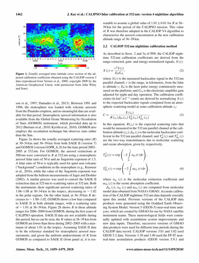
p (z)≈ 1, and in these regionsthe attenuated scattering ratios provide a good proxy for thetrue scattering ratios (i.e., R(z)= (βm(z)+βp(z))/βm(z)).Vernier et al. (2009) calculated R′ from CALIOP 532 nmmeasurements over the tropics and showed anomalously lowvalues (R′< 1) above 34 km, as well as in the lower strato-sphere. Since molecular normalization at 30–34 km impliesR′ should be unity or larger at these altitudes, this findingof non-physical low biases in the CALIOP data stronglysuggested flaws of some sort in the CALIOP calibrationprocedure. In an attempt to eliminate these biases, Vernieret al. (2009) assumed that the 36–39 km altitude region wasaerosol-free and renormalized the CALIOP data set usingthe original R′ values calculated in this region. Figure 1, re-produced from Vernier et al. (2009), shows the latitude–timecross section of their adjusted calibration constant, which canbe interpreted as the R′ that would have been measured at30–34 km if the data had been calibrated in the 36–39 km re-gion. As can be seen, only minor adjustments to the CALIOPV3 calibration are required at the midlatitudes during thistime period, but adjustments of 6–12 % are necessary in thetropics. A similar problem was noted by P09, who founda persistent dip in the tropics in clear-air attenuated scatter-ing ratios (< 1) between 8 and 12 km. This too suggesteddeficiencies in the original CALIOP calibration procedures.

As the mission progressed and understanding of data qual-ity improved, it was realized that the calibration altitudecould be raised to 36–39 km without compromising the qual-ity of the data products. In order to estimate the scatteringratios expected at the increased CALIOP V4 calibration al-titudes, we examined the available stratospheric measure-ments from other satellites. The most extensive and accu-rate measurements of stratospheric aerosols have come fromthe Stratospheric Aerosol and Gas Experiment II (SAGE II)instrument. SAGE II has provided the extinction coefficientprofiles in the stratosphere using the solar occultation tech-nique from 1984 through 2005 (Mauldin et al., 1985; Thoma-

www.atmos-meas-tech.net/11/1459/2018/ Atmos. Meas. Tech., 11, 1459–1479, 2018


Figure 1. Zonally averaged time–latitude cross section of the ad-justed calibration coefficient obtained using the CALIOP version 2data (reproduced from Vernier et al., 2009; copyright 2009 by theAmerican Geophysical Union, with permission from John Wileyand Sons).

son et al., 1997; Damadeo et al., 2013). Between 1991 and1996, the stratosphere was loaded with volcanic aerosolsfrom the Pinatubo eruption, and no meaningful data are avail-able for that period. Stratospheric aerosol information is alsoavailable from the Global Ozone Monitoring by Occultationof Stars (GOMOS) instrument, which provided data up to2012 (Bertaux et al., 2010; Kyrölä et al., 2010). GOMOS alsoemploys the occultation technique but observes stars ratherthan the Sun.

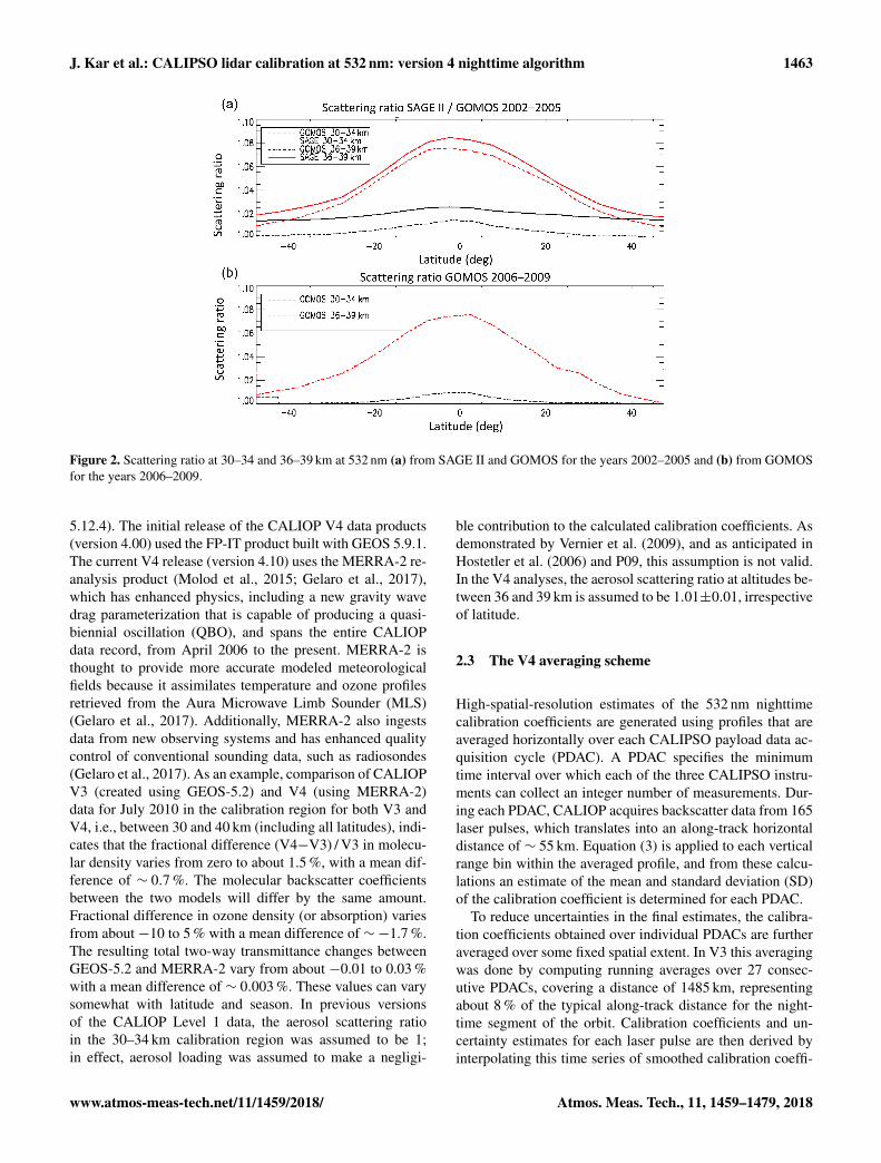
Figure 2a shows the zonally averaged scattering ratio (R)at 30–34 km and 36–39 km from both SAGE II (version 7)and GOMOS (version GOPR_6_0) for the time period 2002–2005 at 532 nm. For GOMOS, the aerosol extinctions at500 nm were converted to R at 532 nm using a stratosphericaerosol lidar ratio of 50 sr and an Ångström exponent of 1.5.A lidar ratio of 50 sr is typically used for quiet non-volcanic(“background”) conditions in the stratosphere (e.g., Kremseret al., 2016), while the value of the Ångström exponent wasadopted from the balloon measurements of Jager and Deshler(2002). A similar process was used to convert the SAGE IIextinction data at 525 nm to scattering ratios at 532 nm. Boththe instruments show significant aerosol scattering ratios of1.06–1.08 at 30–34 km in the tropics, decreasing to ∼ 1.02in the polar regions. On the other hand, at 36–39 km R de-creases to∼ 1.00–1.02. GOMOS shows a low bias comparedto SAGE II in both altitude ranges, with a scattering ratioof ∼ 1.01 at 36–39 km. Figure 2b shows R in these altituderanges for 2006–2009 from GOMOS, during the first years ofCALIPSO operation. SAGE II data are not available duringthis period, but as can be seen, theR values at 36–39 km fromGOMOS are lower than those during 2002–2005 with a max-imum of about 1.01 in the tropics. Assuming SAGE II datato be the reference standard for stratospheric aerosol mea-surements, and given the uniform underestimate of R fromGOMOS as compared to SAGE II (from panel a), it is rea-

sonable to assume a global value of 1.01± 0.01 for R at 36–39 km for the period of the CALIPSO mission. This valueof R was therefore adopted in the CALIOP V4 algorithm tocharacterize the aerosol concentration at the new calibrationaltitude range of 36–39 km.

2.2 CALIOP 532 nm nighttime calibration method

As described in Sects. 2 and 3a of P09, the CALIOP night-time 532 nm calibration coefficients are derived from therange-corrected, gain- and energy-normalized signals, X(z):

X(z)=r2S (z)

E0GA, (2)

where S(z) is the measured backscatter signal in the 532 nmparallel channel; r is the range, in kilometers, from the lidarto altitude z; E0 is the laser pulse energy continuously mea-sured on the platform; andGA is the electronic amplifier gainadjusted for night and day operation. The calibration coeffi-cients (in km3 sr J−1 count) are derived by normalizing X(z)to the expected backscatter signals computed from an atmo-spheric scattering model at some calibration altitude zc:

C =X(zc)

R (zc)βm (zc)T 2m (zc)T

2O3(zc)

. (3)

In this equation, R(zc) is the expected scattering ratio thatwould be measured in the 532 nm parallel channel at the cali-bration altitude (zc); βm (z) is the molecular backscatter coef-ficient in the 532 nm parallel channel; and T 2

m (z) and T 2O3(z)

are the two-way transmittances due to molecular scatteringand ozone absorption, given by, respectively,

T 2m (z)= exp

−2

z∫0

σm (r)dr

,T 2

O3(z)= exp

−2

z∫0

αO3 (r)dr

, (4)

where σm (z) is the molecular extinction coefficient andαO3 (z) is the ozone absorption coefficient.βm (z), σm (z) and αO3 (z) are computed from molecular

model data obtained from NASA’s GMAO. Accurate calibra-tion of the CALIOP nighttime 532 nm data depends cruciallyupon this model. Previous versions of the CALIOP dataproducts were generated using the Goddard Earth Observ-ing System Model, Version 5 (GEOS-5) near-real-time anal-yses, which are created by GMAO for use by NASA satelliteinstrument teams. These meteorological fields were contin-ually updated with assimilation system improvements andnew data inputs. Therefore, successive versions of GMAOdata products were used for different time periods during theCALIOP data record. CALIOP versions 3.01 and 3.02 usedGEOS 5.2 data. Versions 3.30 and 3.40 used the FP-IT near-real-time assimilation products (GEOS version 5.9.1 and



Figure 2. Scattering ratio at 30–34 and 36–39 km at 532 nm (a) from SAGE II and GOMOS for the years 2002–2005 and (b) from GOMOSfor the years 2006–2009.

5.12.4). The initial release of the CALIOP V4 data products(version 4.00) used the FP-IT product built with GEOS 5.9.1.The current V4 release (version 4.10) uses the MERRA-2 re-analysis product (Molod et al., 2015; Gelaro et al., 2017),which has enhanced physics, including a new gravity wavedrag parameterization that is capable of producing a quasi-biennial oscillation (QBO), and spans the entire CALIOPdata record, from April 2006 to the present. MERRA-2 isthought to provide more accurate modeled meteorologicalfields because it assimilates temperature and ozone profilesretrieved from the Aura Microwave Limb Sounder (MLS)(Gelaro et al., 2017). Additionally, MERRA-2 also ingestsdata from new observing systems and has enhanced qualitycontrol of conventional sounding data, such as radiosondes(Gelaro et al., 2017). As an example, comparison of CALIOPV3 (created using GEOS-5.2) and V4 (using MERRA-2)data for July 2010 in the calibration region for both V3 andV4, i.e., between 30 and 40 km (including all latitudes), indi-cates that the fractional difference (V4−V3) / V3 in molecu-lar density varies from zero to about 1.5 %, with a mean dif-ference of ∼ 0.7 %. The molecular backscatter coefficientsbetween the two models will differ by the same amount.Fractional difference in ozone density (or absorption) variesfrom about −10 to 5 % with a mean difference of ∼−1.7 %.The resulting total two-way transmittance changes betweenGEOS-5.2 and MERRA-2 vary from about −0.01 to 0.03 %with a mean difference of ∼ 0.003 %. These values can varysomewhat with latitude and season. In previous versionsof the CALIOP Level 1 data, the aerosol scattering ratioin the 30–34 km calibration region was assumed to be 1;in effect, aerosol loading was assumed to make a negligi-

ble contribution to the calculated calibration coefficients. Asdemonstrated by Vernier et al. (2009), and as anticipated inHostetler et al. (2006) and P09, this assumption is not valid.In the V4 analyses, the aerosol scattering ratio at altitudes be-tween 36 and 39 km is assumed to be 1.01±0.01, irrespectiveof latitude.

2.3 The V4 averaging scheme

High-spatial-resolution estimates of the 532 nm nighttimecalibration coefficients are generated using profiles that areaveraged horizontally over each CALIPSO payload data ac-quisition cycle (PDAC). A PDAC specifies the minimumtime interval over which each of the three CALIPSO instru-ments can collect an integer number of measurements. Dur-ing each PDAC, CALIOP acquires backscatter data from 165laser pulses, which translates into an along-track horizontaldistance of ∼ 55 km. Equation (3) is applied to each verticalrange bin within the averaged profile, and from these calcu-lations an estimate of the mean and standard deviation (SD)of the calibration coefficient is determined for each PDAC.

To reduce uncertainties in the final estimates, the calibra-tion coefficients obtained over individual PDACs are furtheraveraged over some fixed spatial extent. In V3 this averagingwas done by computing running averages over 27 consec-utive PDACs, covering a distance of 1485 km, representingabout 8 % of the typical along-track distance for the night-time segment of the orbit. Calibration coefficients and un-certainty estimates for each laser pulse are then derived byinterpolating this time series of smoothed calibration coeffi-



2012-04-062011-12-182011-09-062011-06-302011-03-162011-01-142010-12-192010-10-092010-07-302010-03-182010-01-162009-11-10Mean profile

SNR

no

rmal

ize

d t

o v

alu

e a

t 3

2 k

m

Altitude (km)

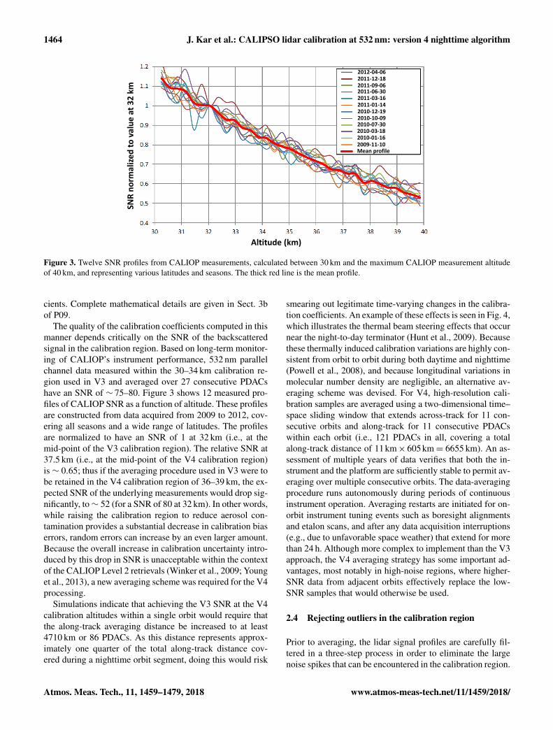
Figure 3. Twelve SNR profiles from CALIOP measurements, calculated between 30 km and the maximum CALIOP measurement altitudeof 40 km, and representing various latitudes and seasons. The thick red line is the mean profile.

cients. Complete mathematical details are given in Sect. 3bof P09.

The quality of the calibration coefficients computed in thismanner depends critically on the SNR of the backscatteredsignal in the calibration region. Based on long-term monitor-ing of CALIOP’s instrument performance, 532 nm parallelchannel data measured within the 30–34 km calibration re-gion used in V3 and averaged over 27 consecutive PDACshave an SNR of ∼ 75–80. Figure 3 shows 12 measured pro-files of CALIOP SNR as a function of altitude. These profilesare constructed from data acquired from 2009 to 2012, cov-ering all seasons and a wide range of latitudes. The profilesare normalized to have an SNR of 1 at 32 km (i.e., at themid-point of the V3 calibration region). The relative SNR at37.5 km (i.e., at the mid-point of the V4 calibration region)is∼ 0.65; thus if the averaging procedure used in V3 were tobe retained in the V4 calibration region of 36–39 km, the ex-pected SNR of the underlying measurements would drop sig-nificantly, to∼ 52 (for a SNR of 80 at 32 km). In other words,while raising the calibration region to reduce aerosol con-tamination provides a substantial decrease in calibration biaserrors, random errors can increase by an even larger amount.Because the overall increase in calibration uncertainty intro-duced by this drop in SNR is unacceptable within the contextof the CALIOP Level 2 retrievals (Winker et al., 2009; Younget al., 2013), a new averaging scheme was required for the V4processing.

Simulations indicate that achieving the V3 SNR at the V4calibration altitudes within a single orbit would require thatthe along-track averaging distance be increased to at least4710 km or 86 PDACs. As this distance represents approx-imately one quarter of the total along-track distance cov-ered during a nighttime orbit segment, doing this would risk

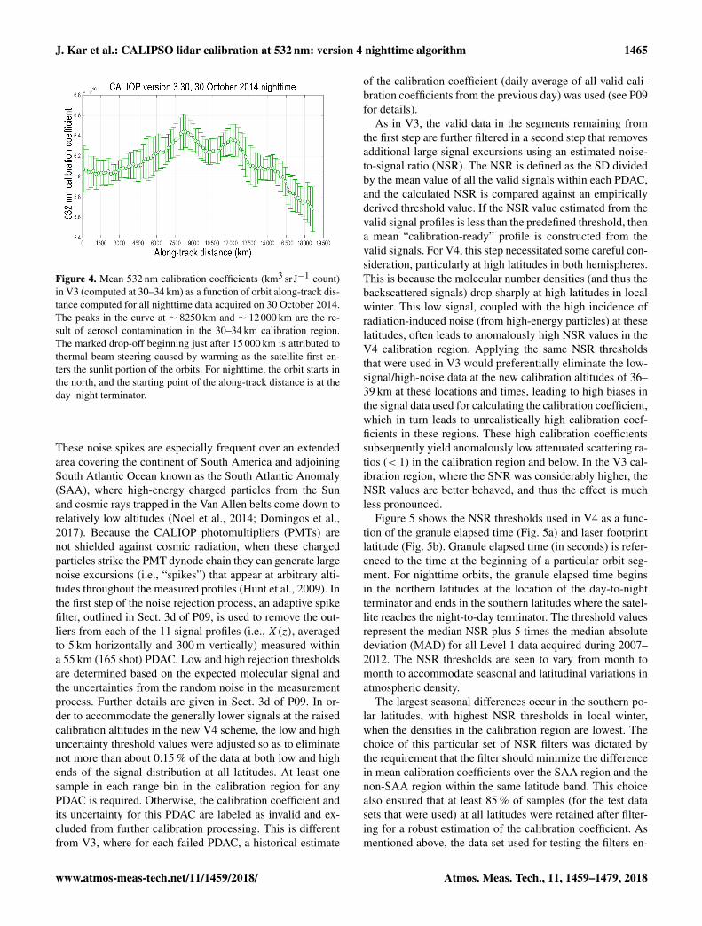
smearing out legitimate time-varying changes in the calibra-tion coefficients. An example of these effects is seen in Fig. 4,which illustrates the thermal beam steering effects that occurnear the night-to-day terminator (Hunt et al., 2009). Becausethese thermally induced calibration variations are highly con-sistent from orbit to orbit during both daytime and nighttime(Powell et al., 2008), and because longitudinal variations inmolecular number density are negligible, an alternative av-eraging scheme was devised. For V4, high-resolution cali-bration samples are averaged using a two-dimensional time–space sliding window that extends across-track for 11 con-secutive orbits and along-track for 11 consecutive PDACswithin each orbit (i.e., 121 PDACs in all, covering a totalalong-track distance of 11km× 605km= 6655 km). An as-sessment of multiple years of data verifies that both the in-strument and the platform are sufficiently stable to permit av-eraging over multiple consecutive orbits. The data-averagingprocedure runs autonomously during periods of continuousinstrument operation. Averaging restarts are initiated for on-orbit instrument tuning events such as boresight alignmentsand etalon scans, and after any data acquisition interruptions(e.g., due to unfavorable space weather) that extend for morethan 24 h. Although more complex to implement than the V3approach, the V4 averaging strategy has some important ad-vantages, most notably in high-noise regions, where higher-SNR data from adjacent orbits effectively replace the low-SNR samples that would otherwise be used.

2.4 Rejecting outliers in the calibration region

Prior to averaging, the lidar signal profiles are carefully fil-tered in a three-step process in order to eliminate the largenoise spikes that can be encountered in the calibration region.



Figure 4. Mean 532 nm calibration coefficients (km3 sr J−1 count)in V3 (computed at 30–34 km) as a function of orbit along-track dis-tance computed for all nighttime data acquired on 30 October 2014.The peaks in the curve at ∼ 8250 km and ∼ 12000 km are the re-sult of aerosol contamination in the 30–34 km calibration region.The marked drop-off beginning just after 15 000 km is attributed tothermal beam steering caused by warming as the satellite first en-ters the sunlit portion of the orbits. For nighttime, the orbit starts inthe north, and the starting point of the along-track distance is at theday–night terminator.

These noise spikes are especially frequent over an extendedarea covering the continent of South America and adjoiningSouth Atlantic Ocean known as the South Atlantic Anomaly(SAA), where high-energy charged particles from the Sunand cosmic rays trapped in the Van Allen belts come down torelatively low altitudes (Noel et al., 2014; Domingos et al.,2017). Because the CALIOP photomultipliers (PMTs) arenot shielded against cosmic radiation, when these chargedparticles strike the PMT dynode chain they can generate largenoise excursions (i.e., “spikes”) that appear at arbitrary alti-tudes throughout the measured profiles (Hunt et al., 2009). Inthe first step of the noise rejection process, an adaptive spikefilter, outlined in Sect. 3d of P09, is used to remove the out-liers from each of the 11 signal profiles (i.e., X(z), averagedto 5 km horizontally and 300 m vertically) measured withina 55 km (165 shot) PDAC. Low and high rejection thresholdsare determined based on the expected molecular signal andthe uncertainties from the random noise in the measurementprocess. Further details are given in Sect. 3d of P09. In or-der to accommodate the generally lower signals at the raisedcalibration altitudes in the new V4 scheme, the low and highuncertainty threshold values were adjusted so as to eliminatenot more than about 0.15 % of the data at both low and highends of the signal distribution at all latitudes. At least onesample in each range bin in the calibration region for anyPDAC is required. Otherwise, the calibration coefficient andits uncertainty for this PDAC are labeled as invalid and ex-cluded from further calibration processing. This is differentfrom V3, where for each failed PDAC, a historical estimate

of the calibration coefficient (daily average of all valid cali-bration coefficients from the previous day) was used (see P09for details).

As in V3, the valid data in the segments remaining fromthe first step are further filtered in a second step that removesadditional large signal excursions using an estimated noise-to-signal ratio (NSR). The NSR is defined as the SD dividedby the mean value of all the valid signals within each PDAC,and the calculated NSR is compared against an empiricallyderived threshold value. If the NSR value estimated from thevalid signal profiles is less than the predefined threshold, thena mean “calibration-ready” profile is constructed from thevalid signals. For V4, this step necessitated some careful con-sideration, particularly at high latitudes in both hemispheres.This is because the molecular number densities (and thus thebackscattered signals) drop sharply at high latitudes in localwinter. This low signal, coupled with the high incidence ofradiation-induced noise (from high-energy particles) at theselatitudes, often leads to anomalously high NSR values in theV4 calibration region. Applying the same NSR thresholdsthat were used in V3 would preferentially eliminate the low-signal/high-noise data at the new calibration altitudes of 36–39 km at these locations and times, leading to high biases inthe signal data used for calculating the calibration coefficient,which in turn leads to unrealistically high calibration coef-ficients in these regions. These high calibration coefficientssubsequently yield anomalously low attenuated scattering ra-tios (< 1) in the calibration region and below. In the V3 cal-ibration region, where the SNR was considerably higher, theNSR values are better behaved, and thus the effect is muchless pronounced.

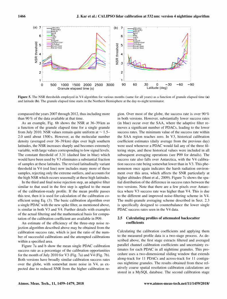
Figure 5 shows the NSR thresholds used in V4 as a func-tion of the granule elapsed time (Fig. 5a) and laser footprintlatitude (Fig. 5b). Granule elapsed time (in seconds) is refer-enced to the time at the beginning of a particular orbit seg-ment. For nighttime orbits, the granule elapsed time beginsin the northern latitudes at the location of the day-to-nightterminator and ends in the southern latitudes where the satel-lite reaches the night-to-day terminator. The threshold valuesrepresent the median NSR plus 5 times the median absolutedeviation (MAD) for all Level 1 data acquired during 2007–2012. The NSR thresholds are seen to vary from month tomonth to accommodate seasonal and latitudinal variations inatmospheric density.

The largest seasonal differences occur in the southern po-lar latitudes, with highest NSR thresholds in local winter,when the densities in the calibration region are lowest. Thechoice of this particular set of NSR filters was dictated bythe requirement that the filter should minimize the differencein mean calibration coefficients over the SAA region and thenon-SAA region within the same latitude band. This choicealso ensured that at least 85 % of samples (for the test datasets that were used) at all latitudes were retained after filter-ing for a robust estimation of the calibration coefficient. Asmentioned above, the data set used for testing the filters en-



Figure 5. The NSR thresholds employed in V4 algorithm for various months (same for all years) as a function of granule elapsed time (a)and latitude (b). The granule elapsed time starts in the Northern Hemisphere at the day-to-night terminator.

compassed the years 2007 through 2012, thus including morethan 90 % of the data available at that time.

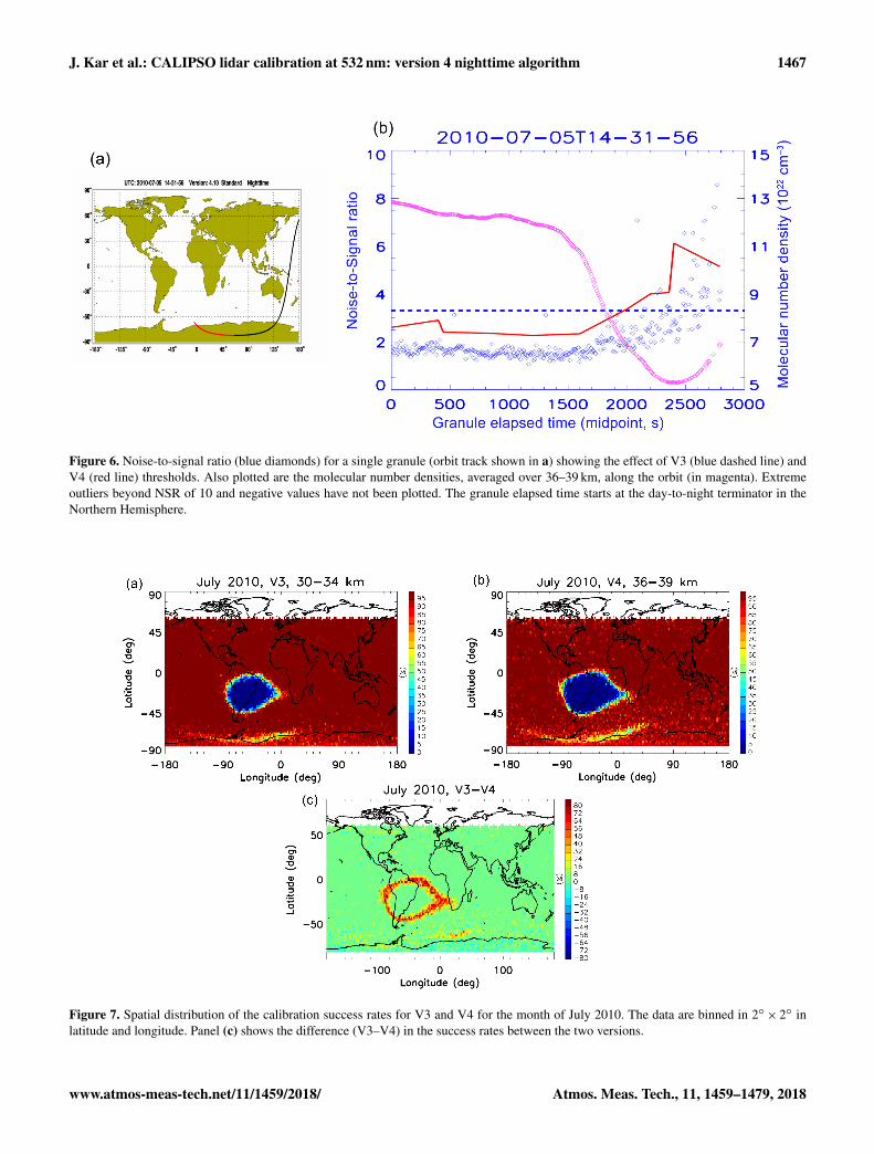
As an example, Fig. 6b shows the NSR at 36–39 km asa function of the granule elapsed time for a single granulefrom July 2010. NSR values remain quite uniform at ∼ 1.5–2.0 until about 1500 s. However, as the molecular numberdensity (averaged over 36–39 km) dips over high southernlatitudes, the NSR increases sharply and becomes extremelyvariable, with large values corresponding to low signal levels.The constant threshold of 3.31 (dashed line in blue) whichwould have been used by V3 eliminates a substantial fractionof samples at these latitudes. The revised latitudinally variantthreshold in V4 (red line) now includes many more of thesesamples, rejecting only the extreme outliers, and accounts forthe high NSR which occurs seasonally at these high latitudes.

In the third and final noise rejection step, an adaptive filtersimilar to that used in the first step is applied to the meanof the calibration-ready profile. If the mean profile passesthis test, then it is used for calculation of the calibration co-efficient using Eq. (3). The basic calibration algorithm overa single PDAC with the new spike filter, as mentioned above,is similar in both V3 and V4. Further details with examplesof the actual filtering and the mathematical basis for compu-tation of the calibration coefficient are available in P09.

An estimate of the efficiency of the three-step noise re-jection algorithm described above may be obtained from thecalibration success rate, which is just the ratio of the num-ber of successful calibrations and the attempted calibrationswithin a specified area.

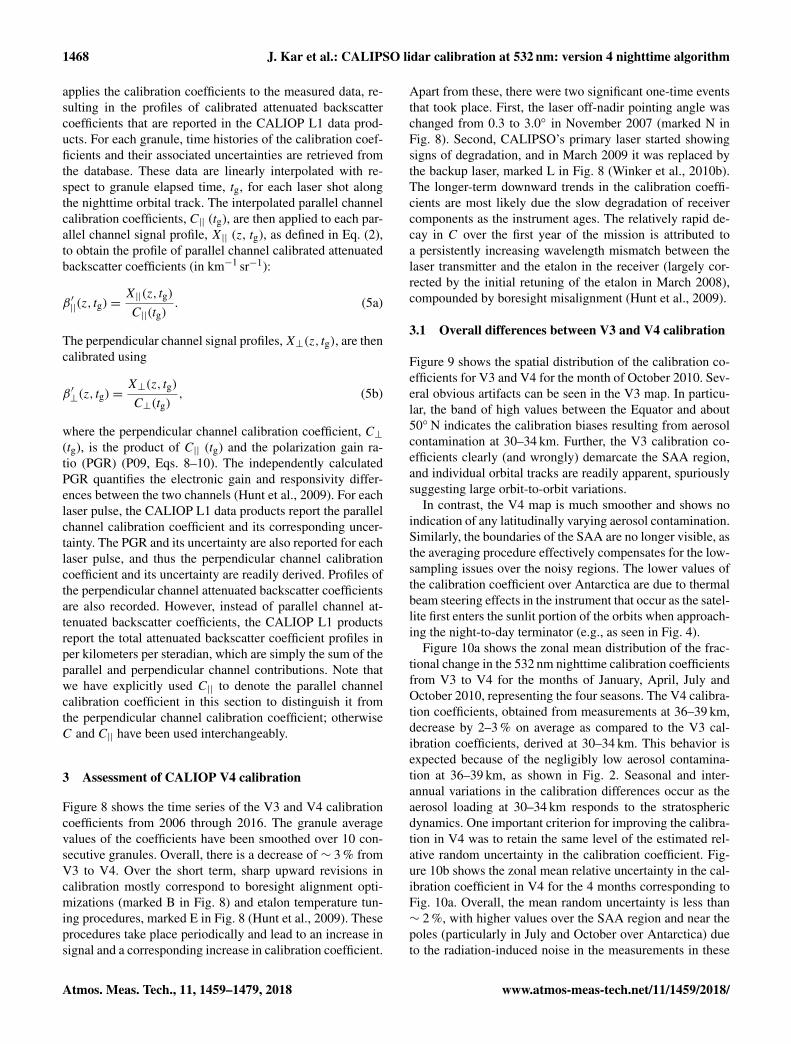
Figure 7a and b show the mean single PDAC calibrationsuccess rate as a percentage of the calibration opportunitiesfor the month of July 2010 for V3 (Fig. 7a) and V4 (Fig. 7b).Both versions have broadly similar calibration success ratesover the globe, with somewhat more noise in V4, as ex-pected due to reduced SNR from the higher calibration re-

gion. Over most of the globe, the success rate is over 90 %in both versions. However, substantially lower success rates(in blue) occur over the SAA, where the adaptive filter re-moves a significant number of PDACs, leading to the lowersuccess rates. The minimum value of the success rate withinthe SAA region reaches zero. In V3, historical calibrationcoefficient estimates (daily average from the previous day)were used whenever a PDAC would fail any of the three fil-tering steps, and these historical values were included in allsubsequent averaging operations (see P09 for details). Thesuccess rate also falls over Antarctica, with the V4 calibra-tion success rate being somewhat lower than in V3. This phe-nomenon once again indicates the harsh radiation environ-ment over this area, which affects the SNR particularly athigher altitudes (Hunt et al., 2009). Figure 7c shows the spa-tial distribution of the difference in success rates between thetwo versions. Note that there are a few pixels over Antarc-tica where V3 success rate was higher than V4. This is dueto the different and improved noise-filtering scheme in V4.The multi-granule averaging scheme described in Sect. 2.3is specifically designed to counterbalance the lower singlePDAC success rates seen in the V4 data.

2.5 Calculating profiles of attenuated backscattercoefficients

Calculating the calibration coefficients and applying themto the measured profile data is a two-stage process. As de-scribed above, the first stage extracts filtered and averagedparallel channel calibration coefficients and uncertainty es-timates for each PDAC in all nighttime granules. This pro-cedure uses a two-dimensional sliding window that extendsalong-track for 11 PDACs and across-track for 11 contigu-ous nighttime granules. The results obtained from these rel-atively coarse spatial resolution calibration calculations arestored in a MySQL database. The second calibration stage



Figure 6. Noise-to-signal ratio (blue diamonds) for a single granule (orbit track shown in a) showing the effect of V3 (blue dashed line) andV4 (red line) thresholds. Also plotted are the molecular number densities, averaged over 36–39 km, along the orbit (in magenta). Extremeoutliers beyond NSR of 10 and negative values have not been plotted. The granule elapsed time starts at the day-to-night terminator in theNorthern Hemisphere.

Figure 7. Spatial distribution of the calibration success rates for V3 and V4 for the month of July 2010. The data are binned in 2◦× 2◦ inlatitude and longitude. Panel (c) shows the difference (V3–V4) in the success rates between the two versions.



applies the calibration coefficients to the measured data, re-sulting in the profiles of calibrated attenuated backscattercoefficients that are reported in the CALIOP L1 data prod-ucts. For each granule, time histories of the calibration coef-ficients and their associated uncertainties are retrieved fromthe database. These data are linearly interpolated with re-spect to granule elapsed time, tg, for each laser shot alongthe nighttime orbital track. The interpolated parallel channelcalibration coefficients, C|| (tg), are then applied to each par-allel channel signal profile, X|| (z, tg), as defined in Eq. (2),to obtain the profile of parallel channel calibrated attenuatedbackscatter coefficients (in km−1 sr−1):

β ′||(z, tg)=

X||(z, tg)

C||(tg). (5a)

The perpendicular channel signal profiles,X⊥(z, tg), are thencalibrated using

β ′⊥(z, tg)=

X⊥(z, tg)

C⊥(tg), (5b)

where the perpendicular channel calibration coefficient, C⊥(tg), is the product of C|| (tg) and the polarization gain ra-tio (PGR) (P09, Eqs. 8–10). The independently calculatedPGR quantifies the electronic gain and responsivity differ-ences between the two channels (Hunt et al., 2009). For eachlaser pulse, the CALIOP L1 data products report the parallelchannel calibration coefficient and its corresponding uncer-tainty. The PGR and its uncertainty are also reported for eachlaser pulse, and thus the perpendicular channel calibrationcoefficient and its uncertainty are readily derived. Profiles ofthe perpendicular channel attenuated backscatter coefficientsare also recorded. However, instead of parallel channel at-tenuated backscatter coefficients, the CALIOP L1 productsreport the total attenuated backscatter coefficient profiles inper kilometers per steradian, which are simply the sum of theparallel and perpendicular channel contributions. Note thatwe have explicitly used C|| to denote the parallel channelcalibration coefficient in this section to distinguish it fromthe perpendicular channel calibration coefficient; otherwiseC and C|| have been used interchangeably.

3 Assessment of CALIOP V4 calibration

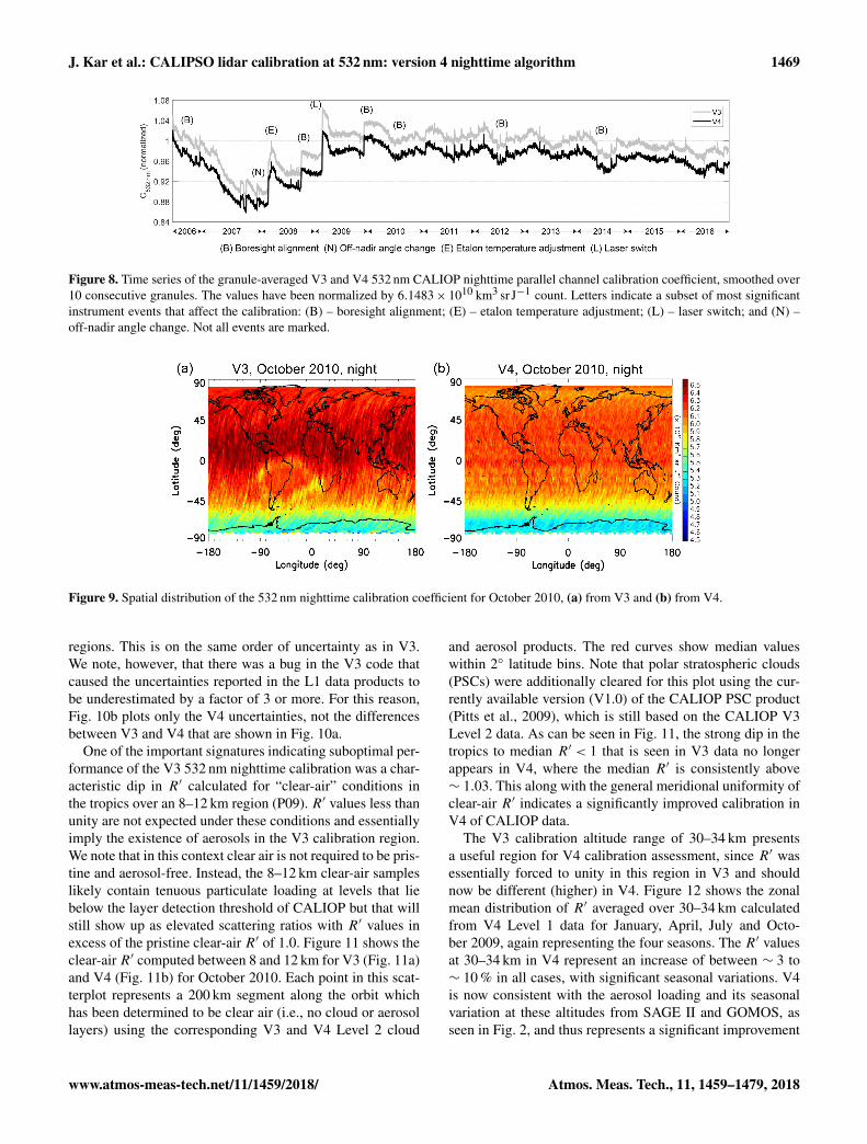
Figure 8 shows the time series of the V3 and V4 calibrationcoefficients from 2006 through 2016. The granule averagevalues of the coefficients have been smoothed over 10 con-secutive granules. Overall, there is a decrease of ∼ 3 % fromV3 to V4. Over the short term, sharp upward revisions incalibration mostly correspond to boresight alignment opti-mizations (marked B in Fig. 8) and etalon temperature tun-ing procedures, marked E in Fig. 8 (Hunt et al., 2009). Theseprocedures take place periodically and lead to an increase insignal and a corresponding increase in calibration coefficient.

Apart from these, there were two significant one-time eventsthat took place. First, the laser off-nadir pointing angle waschanged from 0.3 to 3.0◦ in November 2007 (marked N inFig. 8). Second, CALIPSO’s primary laser started showingsigns of degradation, and in March 2009 it was replaced bythe backup laser, marked L in Fig. 8 (Winker et al., 2010b).The longer-term downward trends in the calibration coeffi-cients are most likely due the slow degradation of receivercomponents as the instrument ages. The relatively rapid de-cay in C over the first year of the mission is attributed toa persistently increasing wavelength mismatch between thelaser transmitter and the etalon in the receiver (largely cor-rected by the initial retuning of the etalon in March 2008),compounded by boresight misalignment (Hunt et al., 2009).

3.1 Overall differences between V3 and V4 calibration

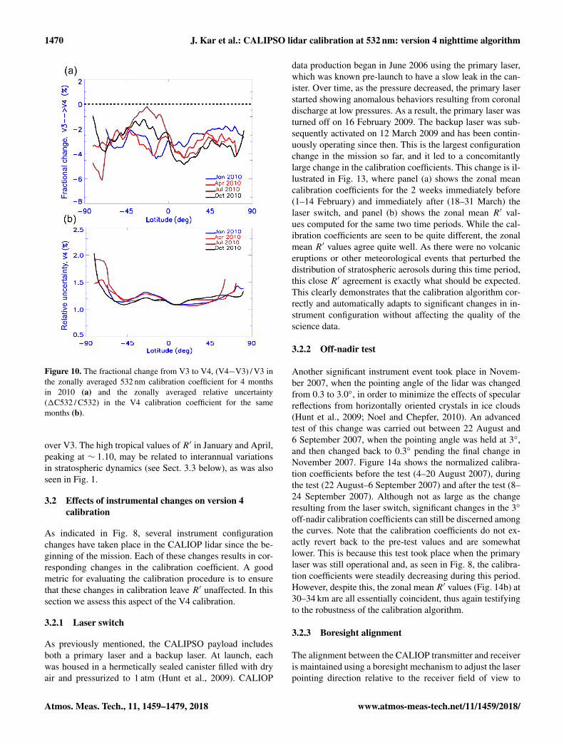
Figure 9 shows the spatial distribution of the calibration co-efficients for V3 and V4 for the month of October 2010. Sev-eral obvious artifacts can be seen in the V3 map. In particu-lar, the band of high values between the Equator and about50◦ N indicates the calibration biases resulting from aerosolcontamination at 30–34 km. Further, the V3 calibration co-efficients clearly (and wrongly) demarcate the SAA region,and individual orbital tracks are readily apparent, spuriouslysuggesting large orbit-to-orbit variations.

In contrast, the V4 map is much smoother and shows noindication of any latitudinally varying aerosol contamination.Similarly, the boundaries of the SAA are no longer visible, asthe averaging procedure effectively compensates for the low-sampling issues over the noisy regions. The lower values ofthe calibration coefficient over Antarctica are due to thermalbeam steering effects in the instrument that occur as the satel-lite first enters the sunlit portion of the orbits when approach-ing the night-to-day terminator (e.g., as seen in Fig. 4).

Figure 10a shows the zonal mean distribution of the frac-tional change in the 532 nm nighttime calibration coefficientsfrom V3 to V4 for the months of January, April, July andOctober 2010, representing the four seasons. The V4 calibra-tion coefficients, obtained from measurements at 36–39 km,decrease by 2–3 % on average as compared to the V3 cal-ibration coefficients, derived at 30–34 km. This behavior isexpected because of the negligibly low aerosol contamina-tion at 36–39 km, as shown in Fig. 2. Seasonal and inter-annual variations in the calibration differences occur as theaerosol loading at 30–34 km responds to the stratosphericdynamics. One important criterion for improving the calibra-tion in V4 was to retain the same level of the estimated rel-ative random uncertainty in the calibration coefficient. Fig-ure 10b shows the zonal mean relative uncertainty in the cal-ibration coefficient in V4 for the 4 months corresponding toFig. 10a. Overall, the mean random uncertainty is less than∼ 2 %, with higher values over the SAA region and near thepoles (particularly in July and October over Antarctica) dueto the radiation-induced noise in the measurements in these



Figure 8. Time series of the granule-averaged V3 and V4 532 nm CALIOP nighttime parallel channel calibration coefficient, smoothed over10 consecutive granules. The values have been normalized by 6.1483× 1010 km3 sr J−1 count. Letters indicate a subset of most significantinstrument events that affect the calibration: (B) – boresight alignment; (E) – etalon temperature adjustment; (L) – laser switch; and (N) –off-nadir angle change. Not all events are marked.

Figure 9. Spatial distribution of the 532 nm nighttime calibration coefficient for October 2010, (a) from V3 and (b) from V4.

regions. This is on the same order of uncertainty as in V3.We note, however, that there was a bug in the V3 code thatcaused the uncertainties reported in the L1 data products tobe underestimated by a factor of 3 or more. For this reason,Fig. 10b plots only the V4 uncertainties, not the differencesbetween V3 and V4 that are shown in Fig. 10a.

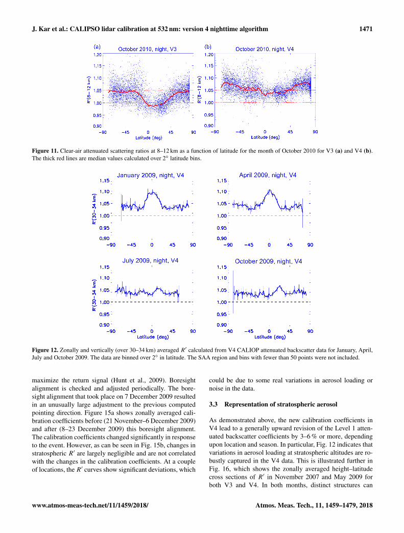
One of the important signatures indicating suboptimal per-formance of the V3 532 nm nighttime calibration was a char-acteristic dip in R′ calculated for “clear-air” conditions inthe tropics over an 8–12 km region (P09). R′ values less thanunity are not expected under these conditions and essentiallyimply the existence of aerosols in the V3 calibration region.We note that in this context clear air is not required to be pris-tine and aerosol-free. Instead, the 8–12 km clear-air sampleslikely contain tenuous particulate loading at levels that liebelow the layer detection threshold of CALIOP but that willstill show up as elevated scattering ratios with R′ values inexcess of the pristine clear-air R′ of 1.0. Figure 11 shows theclear-air R′ computed between 8 and 12 km for V3 (Fig. 11a)and V4 (Fig. 11b) for October 2010. Each point in this scat-terplot represents a 200 km segment along the orbit whichhas been determined to be clear air (i.e., no cloud or aerosollayers) using the corresponding V3 and V4 Level 2 cloud

and aerosol products. The red curves show median valueswithin 2◦ latitude bins. Note that polar stratospheric clouds(PSCs) were additionally cleared for this plot using the cur-rently available version (V1.0) of the CALIOP PSC product(Pitts et al., 2009), which is still based on the CALIOP V3Level 2 data. As can be seen in Fig. 11, the strong dip in thetropics to median R′ < 1 that is seen in V3 data no longerappears in V4, where the median R′ is consistently above∼ 1.03. This along with the general meridional uniformity ofclear-air R′ indicates a significantly improved calibration inV4 of CALIOP data.

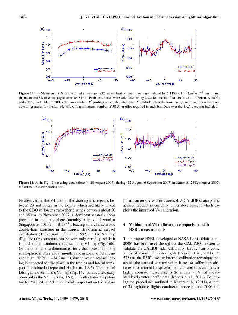
The V3 calibration altitude range of 30–34 km presentsa useful region for V4 calibration assessment, since R′ wasessentially forced to unity in this region in V3 and shouldnow be different (higher) in V4. Figure 12 shows the zonalmean distribution of R′ averaged over 30–34 km calculatedfrom V4 Level 1 data for January, April, July and Octo-ber 2009, again representing the four seasons. The R′ valuesat 30–34 km in V4 represent an increase of between ∼ 3 to∼ 10 % in all cases, with significant seasonal variations. V4is now consistent with the aerosol loading and its seasonalvariation at these altitudes from SAGE II and GOMOS, asseen in Fig. 2, and thus represents a significant improvement



Figure 10. The fractional change from V3 to V4, (V4−V3) / V3 inthe zonally averaged 532 nm calibration coefficient for 4 monthsin 2010 (a) and the zonally averaged relative uncertainty(1C532 / C532) in the V4 calibration coefficient for the samemonths (b).

over V3. The high tropical values of R′ in January and April,peaking at ∼ 1.10, may be related to interannual variationsin stratospheric dynamics (see Sect. 3.3 below), as was alsoseen in Fig. 1.

3.2 Effects of instrumental changes on version 4calibration

As indicated in Fig. 8, several instrument configurationchanges have taken place in the CALIOP lidar since the be-ginning of the mission. Each of these changes results in cor-responding changes in the calibration coefficient. A goodmetric for evaluating the calibration procedure is to ensurethat these changes in calibration leave R′ unaffected. In thissection we assess this aspect of the V4 calibration.

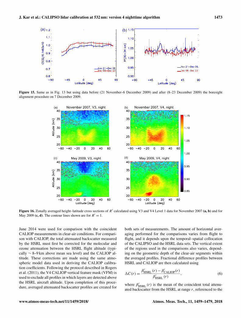
3.2.1 Laser switch

As previously mentioned, the CALIPSO payload includesboth a primary laser and a backup laser. At launch, eachwas housed in a hermetically sealed canister filled with dryair and pressurized to 1 atm (Hunt et al., 2009). CALIOP

data production began in June 2006 using the primary laser,which was known pre-launch to have a slow leak in the can-ister. Over time, as the pressure decreased, the primary laserstarted showing anomalous behaviors resulting from coronaldischarge at low pressures. As a result, the primary laser wasturned off on 16 February 2009. The backup laser was sub-sequently activated on 12 March 2009 and has been contin-uously operating since then. This is the largest configurationchange in the mission so far, and it led to a concomitantlylarge change in the calibration coefficients. This change is il-lustrated in Fig. 13, where panel (a) shows the zonal meancalibration coefficients for the 2 weeks immediately before(1–14 February) and immediately after (18–31 March) thelaser switch, and panel (b) shows the zonal mean R′ val-ues computed for the same two time periods. While the cal-ibration coefficients are seen to be quite different, the zonalmean R′ values agree quite well. As there were no volcaniceruptions or other meteorological events that perturbed thedistribution of stratospheric aerosols during this time period,this close R′ agreement is exactly what should be expected.This clearly demonstrates that the calibration algorithm cor-rectly and automatically adapts to significant changes in in-strument configuration without affecting the quality of thescience data.

3.2.2 Off-nadir test

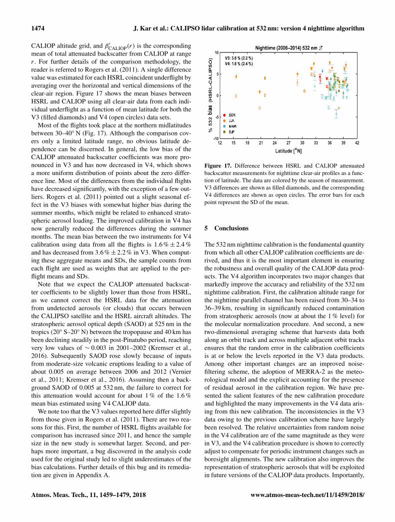
Another significant instrument event took place in Novem-ber 2007, when the pointing angle of the lidar was changedfrom 0.3 to 3.0◦, in order to minimize the effects of specularreflections from horizontally oriented crystals in ice clouds(Hunt et al., 2009; Noel and Chepfer, 2010). An advancedtest of this change was carried out between 22 August and6 September 2007, when the pointing angle was held at 3◦,and then changed back to 0.3◦ pending the final change inNovember 2007. Figure 14a shows the normalized calibra-tion coefficients before the test (4–20 August 2007), duringthe test (22 August–6 September 2007) and after the test (8–24 September 2007). Although not as large as the changeresulting from the laser switch, significant changes in the 3◦

off-nadir calibration coefficients can still be discerned amongthe curves. Note that the calibration coefficients do not ex-actly revert back to the pre-test values and are somewhatlower. This is because this test took place when the primarylaser was still operational and, as seen in Fig. 8, the calibra-tion coefficients were steadily decreasing during this period.However, despite this, the zonal mean R′ values (Fig. 14b) at30–34 km are all essentially coincident, thus again testifyingto the robustness of the calibration algorithm.

3.2.3 Boresight alignment

The alignment between the CALIOP transmitter and receiveris maintained using a boresight mechanism to adjust the laserpointing direction relative to the receiver field of view to



Figure 11. Clear-air attenuated scattering ratios at 8–12 km as a function of latitude for the month of October 2010 for V3 (a) and V4 (b).The thick red lines are median values calculated over 2◦ latitude bins.

Figure 12. Zonally and vertically (over 30–34 km) averaged R′ calculated from V4 CALIOP attenuated backscatter data for January, April,July and October 2009. The data are binned over 2◦ in latitude. The SAA region and bins with fewer than 50 points were not included.

maximize the return signal (Hunt et al., 2009). Boresightalignment is checked and adjusted periodically. The bore-sight alignment that took place on 7 December 2009 resultedin an unusually large adjustment to the previous computedpointing direction. Figure 15a shows zonally averaged cali-bration coefficients before (21 November–6 December 2009)and after (8–23 December 2009) this boresight alignment.The calibration coefficients changed significantly in responseto the event. However, as can be seen in Fig. 15b, changes instratospheric R′ are largely negligible and are not correlatedwith the changes in the calibration coefficients. At a coupleof locations, theR′ curves show significant deviations, which

could be due to some real variations in aerosol loading ornoise in the data.

3.3 Representation of stratospheric aerosol

As demonstrated above, the new calibration coefficients inV4 lead to a generally upward revision of the Level 1 atten-uated backscatter coefficients by 3–6 % or more, dependingupon location and season. In particular, Fig. 12 indicates thatvariations in aerosol loading at stratospheric altitudes are ro-bustly captured in the V4 data. This is illustrated further inFig. 16, which shows the zonally averaged height–latitudecross sections of R′ in November 2007 and May 2009 forboth V3 and V4. In both months, distinct structures can



Figure 13. (a) Means and SDs of the zonally averaged 532 nm calibration coefficients normalized by 6.1483× 1010 km3 sr J−1 count, and(b) mean and SD of R′ averaged over 30–34 km. Both time series were calculated using 2 weeks’ worth of data before (1–14 February 2009)and after (18–31 March 2009) the laser switch. R′ profiles were calculated over 2◦ latitude intervals from each granule and then averagedover all granules for the latitude bin, with a minimum number of 50 R′ profiles required in each bin. Data over the SAA were not included.

Figure 14. As in Fig. 13 but using data before (4–20 August 2007), during (22 August–6 September 2007) and after (8–24 September 2007)the off-nadir laser-pointing test.

be observed in the V4 data in the stratospheric regions be-tween 20 and 30 km in the tropics which are likely linkedto the QBO of lower stratospheric winds between about 20and 35 km. In November 2007, a dominant westerly shearprevailed in the stratosphere (monthly mean zonal wind atSingapore at 10 hPa= 18 ms−1), leading to a characteristicdouble-horn structure in the tropical stratospheric aerosoldistribution (Trepte and Hitchman, 1992). In the V3 map(Fig. 16a) this structure can be seen only partially, while itis much more prominent and clear in the V4 map (Fig. 16b).On the other hand, a dominant easterly shear prevailed in thestratosphere in May 2009 (monthly mean zonal wind at Sin-gapore at 10hPa=−34.2 ms−1), during which aerosol loft-ing is expected to take place in the tropics and lateral trans-port is inhibited (Trepte and Hitchman, 1992). The aerosollofting is not seen in the V3 map (Fig. 16c) but is quite clearlyobserved in the V4 map (Fig. 16d). This illustrates the poten-tial for V4 CALIOP data to provide important and robust in-

formation on stratospheric aerosol. A CALIOP stratosphericaerosol product is currently under development which ex-ploits the improved V4 calibration.

4 Validation of V4 calibration: comparisons withHSRL measurements

The airborne HSRL developed at NASA LaRC (Hair et al.,2008) has been used throughout the CALIPSO mission tovalidate the CALIOP lidar calibration through an ongoingseries of coincident underflights (Rogers et al., 2011). At532 nm, the HSRL uses an internal calibration technique thatavoids the aerosol contamination issues at calibration alti-tudes encountered by spaceborne lidars and thus can deliverhighly accurate measurements (to within ∼ 1 %) of attenu-ated backscatter coefficients (Rogers et al., 2011). Follow-ing the procedures outlined in Rogers et al. (2011), a totalof 35 nighttime flights conducted between June 2006 and



Figure 15. Same as in Fig. 13 but using data before (21 November–6 December 2009) and after (8–23 December 2009) the boresightalignment procedure on 7 December 2009.

Figure 16. Zonally averaged height–latitude cross sections of R′ calculated using V3 and V4 Level 1 data for November 2007 (a, b) and forMay 2009 (c, d). The contour lines shown are for R′ = 1.

June 2014 were used for comparison with the coincidentCALIOP measurements in clear-air conditions. For compari-son with CALIOP, the total attenuated backscatter measuredby the HSRL must first be corrected for the molecular andozone attenuation between the HSRL flight altitude (typi-cally ∼ 8–9 km above mean sea level) and the CALIOP al-titude. These corrections are made using the same atmo-spheric model data used in deriving the CALIOP calibra-tion coefficients. Following the protocol described in Rogerset al. (2011), the V4 CALIOP vertical feature mask (VFM) isused to exclude all profiles in which layers are detected abovethe HSRL aircraft altitude. Upon completion of this proce-dure, averaged attenuated backscatter profiles are created for

both sets of measurements. The amount of horizontal aver-aging performed for the comparisons varies from flight toflight, and it depends upon the temporal–spatial collocationof the CALIPSO and the HSRL data sets. The vertical extentof the regions used in the comparisons also varies, depend-ing on the geometric depth of the clear-air segments withinthe averaged profiles. Fractional difference profiles betweenHSRL and CALIOP are then calculated using

1C(r)=β ′HSRL (r)−β

′

CALIOP(r)

β ′HSRL (r), (6)

where β ′HSRL (r) is the mean of the coincident total attenu-ated backscatter from the HSRL at range r , referenced to the



CALIOP altitude grid, and β ′CALIOP(r) is the correspondingmean of total attenuated backscatter from CALIOP at ranger . For further details of the comparison methodology, thereader is referred to Rogers et al. (2011). A single differencevalue was estimated for each HSRL coincident underflight byaveraging over the horizontal and vertical dimensions of theclear-air region. Figure 17 shows the mean biases betweenHSRL and CALIOP using all clear-air data from each indi-vidual underflight as a function of mean latitude for both theV3 (filled diamonds) and V4 (open circles) data sets.

Most of the flights took place at the northern midlatitudesbetween 30–40◦ N (Fig. 17). Although the comparison cov-ers only a limited latitude range, no obvious latitude de-pendence can be discerned. In general, the low bias of theCALIOP attenuated backscatter coefficients was more pro-nounced in V3 and has now decreased in V4, which showsa more uniform distribution of points about the zero differ-ence line. Most of the differences from the individual flightshave decreased significantly, with the exception of a few out-liers. Rogers et al. (2011) pointed out a slight seasonal ef-fect in the V3 biases with somewhat higher bias during thesummer months, which might be related to enhanced strato-spheric aerosol loading. The improved calibration in V4 hasnow generally reduced the differences during the summermonths. The mean bias between the two instruments for V4calibration using data from all the flights is 1.6%± 2.4 %and has decreased from 3.6%± 2.2% in V3. When comput-ing these aggregate means and SDs, the sample counts fromeach flight are used as weights that are applied to the per-flight means and SDs.

Note that we expect the CALIOP attenuated backscat-ter coefficients to be slightly lower than those from HSRL,as we cannot correct the HSRL data for the attenuationfrom undetected aerosols (or clouds) that occurs betweenthe CALIPSO satellite and the HSRL aircraft altitudes. Thestratospheric aerosol optical depth (SAOD) at 525 nm in thetropics (20◦ S–20◦ N) between the tropopause and 40 km hasbeen declining steadily in the post-Pinatubo period, reachingvery low values of ∼ 0.003 in 2001–2002 (Kremser et al.,2016). Subsequently SAOD rose slowly because of inputsfrom moderate-size volcanic eruptions leading to a value ofabout 0.005 on average between 2006 and 2012 (Vernieret al., 2011; Kremser et al., 2016). Assuming then a back-ground SAOD of 0.005 at 532 nm, the failure to correct forthis attenuation would account for about 1 % of the 1.6 %mean bias estimated using V4 CALIOP data.

We note too that the V3 values reported here differ slightlyfrom those given in Rogers et al. (2011). There are two rea-sons for this. First, the number of HSRL flights available forcomparison has increased since 2011, and hence the samplesize in the new study is somewhat larger. Second, and per-haps more important, a bug discovered in the analysis codeused for the original study led to slight underestimates of thebias calculations. Further details of this bug and its remedia-tion are given in Appendix A.

Figure 17. Difference between HSRL and CALIOP attenuatedbackscatter measurements for nighttime clear-air profiles as a func-tion of latitude. The data are colored by the season of measurement.V3 differences are shown as filled diamonds, and the correspondingV4 differences are shown as open circles. The error bars for eachpoint represent the SD of the mean.

5 Conclusions

The 532 nm nighttime calibration is the fundamental quantityfrom which all other CALIOP calibration coefficients are de-rived, and thus it is the most important element in ensuringthe robustness and overall quality of the CALIOP data prod-ucts. The V4 algorithm incorporates two major changes thatmarkedly improve the accuracy and reliability of the 532 nmnighttime calibration. First, the calibration altitude range forthe nighttime parallel channel has been raised from 30–34 to36–39 km, resulting in significantly reduced contaminationfrom stratospheric aerosols (now at about the 1 % level) forthe molecular normalization procedure. And second, a newtwo-dimensional averaging scheme that harvests data bothalong an orbit track and across multiple adjacent orbit tracksensures that the random error in the calibration coefficientsis at or below the levels reported in the V3 data products.Among other important changes are an improved noise-filtering scheme, the adoption of MERRA-2 as the meteo-rological model and the explicit accounting for the presenceof residual aerosol in the calibration region. We have pre-sented the salient features of the new calibration procedureand highlighted the many improvements in the V4 data aris-ing from this new calibration. The inconsistencies in the V3data owing to the previous calibration scheme have largelybeen resolved. The relative uncertainties from random noisein the V4 calibration are of the same magnitude as they werein V3, and the V4 calibration procedure is shown to correctlyadjust to compensate for periodic instrument changes such asboresight alignments. The new calibration also improves therepresentation of stratospheric aerosols that will be exploitedin future versions of the CALIOP data products. Importantly,



validation of the V4 nighttime calibration coefficients usingthe coincident HSRL measurements at northern midlatitudesindicates an agreement to within ∼ 1.6%± 2.4 %, reducedfrom 3.6%± 2.2% in V3, indicating a robust enhancementin calibration accuracy. Overall, a significant improvement inCALIOP primary calibration has been achieved in V4 whichwill result in corresponding improvements in the downstreamLevel 1 and Level 2 CALIOP products. In particular, the at-tenuated backscatter values increase by about 2–3 % on av-erage, which enables increased detection of tenuous layersby the Level 2 algorithm, particularly in the stratosphere.The improvements in stratospheric aerosol retrievals will beinvaluable for cross-validation of the stratospheric aerosolproducts from other instruments, such as the StratosphericAerosol and Gas Experiment III on International Space Sta-tion (SAGE III-ISS), and are expected to lead to a better un-derstanding of climate-related issues.

Data availability. CALIPSO lidar Level 1b data products arepublicly available at the Atmospheric Science Data Center atNASA LaRC (https://eosweb.larc.nasa.gov/project/calipso/calipso_table; National Aeronautics and Space Administration, 2018a)and at the AERIS/ICARE Data and Services Center (http://www.icare.univ-lille1.fr). The SAGE II data products are also pub-licly available at the Atmospheric Science Data Center (https://eosweb.larc.nasa.gov/project/sage2/sage2_table; National Aero-nautics and Space Administration, 2018b). HSRL data areavailable by request from the authors (Mark Vaughan [email protected]) or from the NASA-Langley HSRLteam (John Hair at [email protected]).


https://eosweb.larc.nasa.gov/project/calipso/calipso_table


http://www.icare.univ-lille1.fr

http://www.icare.univ-lille1.fr

https://eosweb.larc.nasa.gov/project/sage2/sage2_table



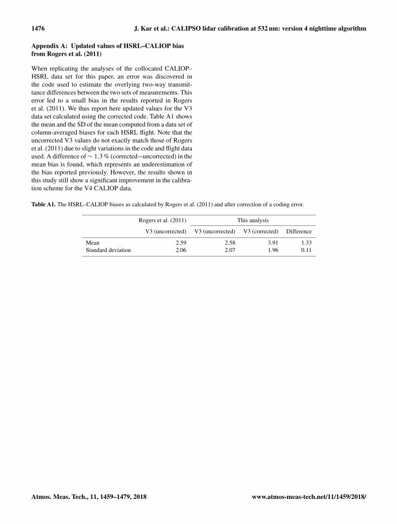
Appendix A: Updated values of HSRL–CALIOP biasfrom Rogers et al. (2011)

When replicating the analyses of the collocated CALIOP–HSRL data set for this paper, an error was discovered inthe code used to estimate the overlying two-way transmit-tance differences between the two sets of measurements. Thiserror led to a small bias in the results reported in Rogerset al. (2011). We thus report here updated values for the V3data set calculated using the corrected code. Table A1 showsthe mean and the SD of the mean computed from a data set ofcolumn-averaged biases for each HSRL flight. Note that theuncorrected V3 values do not exactly match those of Rogerset al. (2011) due to slight variations in the code and flight dataused. A difference of∼ 1.3 % (corrected−uncorrected) in themean bias is found, which represents an underestimation ofthe bias reported previously. However, the results shown inthis study still show a significant improvement in the calibra-tion scheme for the V4 CALIOP data.

Table A1. The HSRL–CALIOP biases as calculated by Rogers et al. (2011) and after correction of a coding error.

Rogers et al. (2011) This analysis

V3 (uncorrected) V3 (uncorrected) V3 (corrected) Difference

Mean 2.59 2.58 3.91 1.33Standard deviation 2.06 2.07 1.96 0.11



Competing interests. Authors Charles R. Trepte and Jacques Pelonare co-guest-editors for the “CALIPSO version 4 algorithms anddata products” special issue in Atmospheric Measurement Tech-niques but did not participate in any aspects of the editorial reviewof this paper. All other authors declare that they have no conflicts ofinterest.

Special issue statement. This article is part of the special issue“CALIPSO version 4 algorithms and data products”. It is not af-filiated with a conference.

Acknowledgements. We are grateful to Laurent Blanot and theGOMOS team for providing us with the GOMOS data. Figure 1was reproduced (copyright 2009 American Geophysical Union)with permission from John Wiley and Sons. This paper is dedicatedto the memory of William H. Hunt. The referees are thanked foruseful comments which helped improve the quality of the paper.

Edited by: Vassilis AmiridisReviewed by: Franco Marenco and two anonymous referees

References

Behrenfeld, M. J., Hu, Y., O’Malley, R. T., Boss, E. S.,Hostetler, C. A., Siegel, D. A., Sarmiento, J. L., Schulien, J.,Hair, J. W., Lu, X., Rodier, S., and Scarino, A. J.: An-nual boom – bust cycles of polar phytoplankton biomassrevealed by space-based lidar, Nat. Geosci., 10, 118–122,https://doi.org/10.1038/ngeo2861, 2017.

Bertaux, J. L., Kyrölä, E., Fussen, D., Hauchecorne, A., Dalaudier,F., Sofieva, V., Tamminen, J., Vanhellemont, F., Fanton d’Andon,O., Barrot, G., Mangin, A., Blanot, L., Lebrun, J. C., Pérot,K., Fehr, T., Saavedra, L., Leppelmeier, G. W., and Fraisse, R.:Global ozone monitoring by occultation of stars: an overviewof GOMOS measurements on ENVISAT, Atmos. Chem. Phys.,10, 12091–12148, https://doi.org/10.5194/acp-10-12091-2010,2010.

Damadeo, R. P., Zawodny, J. M., Thomason, L. W., and Iyer, N.:SAGE version 7.0 algorithm: application to SAGE II, Atmos.Meas. Tech., 6, 3539–3561, https://doi.org/10.5194/amt-6-3539-2013, 2013.

Domingos, J., Jault, D., Pais, M. A., and Mandea, M.: The SouthAtlantic Anomaly throughout the solar cycle, Earth Planet. Sc.Lett., 473, 154–163, https://doi.org/10.1016/j.epsl.2017.06.004,2017.

Garnier, A., Scott, N. A., Pelon, J., Armante, R., Crépeau, L.,Six, B., and Pascal, N.: Long-term assessment of the CALIPSOImaging Infrared Radiometer (IIR) calibration and stabilitythrough simulated and observed comparisons with MODIS/Aquaand SEVIRI/Meteosat, Atmos. Meas. Tech., 10, 1403–1424,https://doi.org/10.5194/amt-10-1403-2017, 2017.

Gelaro, R., McCarty, W., Suarez, M. J., Todling, R., Molod, A.,Takacs, L., Randles, C. A., Darmenov, A., Bosilovich, M. G.,Reichle, R., Wargan, K., Coy, L., Cullather, R., Draper, C.,Akella, S., Buchard, V., Conaty, A., Da Silva, A. M.,Gu, W., Kim, G.-K., Koster, R., Lucchesi, R., Markova, D.,

Nielsen, J. E., Partyka, G., Pawson, S., Putman, W., Rie-necker, M., Schubert, S. C., Sienkiewicz, M., and Zhao, B.:The Modern-Era Retrospective Analysis for Research and Ap-plications, Version 2 (MERRA-2), J. Climate, 30, 5419–5454,https://doi.org/10.1175/JCLI-D-16-0758.1, 2017.

Getzewich, B., Vaughan, M., Hunt, W., Avery, M., Tackett, J.,Kar, J., and Lee, K.-P.: CALIPSO Lidar Calibration at 532 nm:Version 4 Daytime Algorithm, in preparation, 2018.

Gimmestad, G., Forrister, H., Grigas, T., and O’Dowd, C., Com-parisons of aerosol backscatter using satellite and ground lidars:Implications for calibrating and validating space borne lidar, Sci.Rep.-UK, 7, 42337, https://doi.org/10.1038/srep42337, 2017.

Hair, J. W., Hostetler, C. A., Cook, A. L., Harper, D. B., Fer-rare, R. A., Mack, T. L., Welch, W., Isquierdo, L. R., and Ho-vis, F. E.: Airborne High Spectral Resolution Lidar for pro-filing aerosol optical properties, Appl. Optics, 47, 6734–6752,https://doi.org/10.1364/AO.47.006734, 2008.

Hostetler, C. A., Liu, Z., Reagan, J., Vaughan, M., Winker, D., Os-born, M., Hunt, W. H., Powell, K. A., and Trepte, C.: CALIOPAlgorithm Theoretical Basis Document, Calibration and Level 1Data Products, PC-SCI-201, NASA Langley Research Center,Hampton, VA 23681, 66 pp., available at: http://www-calipso.larc.nasa.gov/resources/project_documentation.php (last access:12 March 2018), 2006.

Hu, Y., Winker, D., Vaughan, M., Lin, B., Omar, A., Trepte, C.,Flittner, D., Yang, P., Sun, W., Liu, Z., Wang, Z., Young, S.,Stamnes, K., Huang, J., Kuehn, R., Baum, B., andHolz, R.: CALIPSO/CALIOP Cloud Phase Discrimina-tion Algorithm, J. Atmos. Ocean. Tech., 26, 2293–2309,https://doi.org/10.1175/2009JTECHA1280.1, 2009.

Hunt, W. H., Winker, D. M., Vaughan, M. A., Powell, K. A.,Lucker, P. L., and Weimer, C.: CALIPSO Lidar description andperformance assessment, J. Atmos. Ocean. Tech., 26, 1214–1228, https://doi.org/10.1175/2009JTECHA1223.1, 2009.

Jager, H. and Deshler, T.: Lidar backscatter to extinction, mass andarea conversions for stratospheric aerosols based on midlatitudeballoonborne size distribution measurements, Geophys. Res.Lett., 29, 1929, https://doi.org/10.1029/2002GL015609, 2002.

Kremser, S., Thomason, L. W., von Hobe, M., Hermann, M., Desh-ler, T., Timmreck, C., Toohey, M., Stenke, A., Schwarz, J. P.,Weigel, R., Fueglistaler, S., Prata, F. J., Vernier, J.-P.,Schlager, H., Barnes, J. E., Antuna-Marrero, J.-C., Fairlie, D.,Palm, M., Mahieu, E., Notholt, J., Rex, M., Bingen, C., Vanhelle-mont, F., Bourassa, A., Plane, J. M. C., Kolcke, D., Carn, S. A.,Clarisse, L., Trickl, T., Neely, R., James, A. D., Rieger, L., Wil-son, J. C., and Meland, B.: Stratospheric aerosol-Observations,processes and impact on climate, Rev. Geophys., 54, 278–335,https://doi.org/10.1002/2015RG000511, 2016.

Kyrölä, E., Tamminen, J., Sofieva, V., Bertaux, J. L., Hauchecorne,A., Dalaudier, F., Fussen, D., Vanhellemont, F., Fanton d’Andon,O., Barrot, G., Guirlet, M., Mangin, A., Blanot, L., Fehr, T.,Saavedra de Miguel, L., and Fraisse, R.: Retrieval of atmosphericparameters from GOMOS data, Atmos. Chem. Phys., 10, 11881–11903, https://doi.org/10.5194/acp-10-11881-2010, 2010.

Liu, Z. Vaughan, M., Winker, D., Kittaka, C., Getzewich, B.,Kuehn, R., Omar, A., Powell, K., Trepte, C., and Hostetler, C.:The CALIPSO lidar cloud and aerosol discrimination: Version 2Algorithm and initial assessment of performance, J. Atmos.Ocean. Tech., 26, 1198–1212, 2009.


https://doi.org/10.1038/ngeo2861

https://doi.org/10.5194/acp-10-12091-2010

https://doi.org/10.5194/amt-6-3539-2013

https://doi.org/10.5194/amt-6-3539-2013

https://doi.org/10.1016/j.epsl.2017.06.004

https://doi.org/10.5194/amt-10-1403-2017

https://doi.org/10.1175/JCLI-D-16-0758.1

https://doi.org/10.1038/srep42337

https://doi.org/10.1364/AO.47.006734

http://www-calipso.larc.nasa.gov/resources/project_documentation.php

http://www-calipso.larc.nasa.gov/resources/project_documentation.php

https://doi.org/10.1175/2009JTECHA1280.1


https://doi.org/10.1029/2002GL015609

https://doi.org/10.1002/2015RG000511

https://doi.org/10.5194/acp-10-11881-2010


Mamouri, R. E., Amiridis, V., Papayannis, A., Giannakaki, E.,Tsaknakis, G., and Balis, D. S.: Validation of CALIPSO space-borne-derived attenuated backscatter coefficient profiles using aground-based lidar in Athens, Greece, Atmos. Meas. Tech., 2,513–522, https://doi.org/10.5194/amt-2-513-2009, 2009.

Mauldin III, L. E., Zaun, N, H., McCormick, M. P., Guy, J. H.,and Vaughan, W. R.: Stratospheric aerosol and gas experiment IIinstrument: A functional description, Opt. Eng., 24, 307–312,1985.

Molod, A., Takacs, L., Suarez, M., and Bacmeister, J.: Developmentof the GEOS-5 atmospheric general circulation model: evolutionfrom MERRA to MERRA2, Geosci. Model Dev., 8, 1339–1356,https://doi.org/10.5194/gmd-8-1339-2015, 2015.

Mona, L., Pappalardo, G., Amodeo, A., D’Amico, G., Madonna,F., Boselli, A., Giunta, A., Russo, F., and Cuomo, V.: Oneyear of CNR-IMAA multi-wavelength Raman lidar measure-ments in coincidence with CALIPSO overpasses: Level 1products comparison, Atmos. Chem. Phys., 9, 7213–7228,https://doi.org/10.5194/acp-9-7213-2009, 2009.

National Aeronautics and Space Administration: CALIPSO dataand information, available at: https://eosweb.larc.nasa.gov/project/calipso/calipso_table, last access: 12 March 2018a.

National Aeronautics and Space Administration: SAGE II data andinformation, available at: https://eosweb.larc.nasa.gov/project/sage2/sage2_table, last access: 12 March 2018b.

Omar, A., Winker, D. M., Kittaka, C., Vaughan, M., Liu, Z.,Hu, Y., Trepte, C. R., Rogers, R. R., Ferrare, R. A., Lee, K-P,Kuehn, R. E., and Hosteler, C. A.: The CALIPSO automatedaerosol classification and lidar ratio selection algorithm, J. At-mos. Ocean. Tech., 26, 1994–2014, 2009.

Noel, V. and Chepfer, H.: A global view of horizontally-orientedcrystals in ice clouds from CALIPSO, J. Geophys. Res., 115,D00H23, https://doi.org/10.1029/2009JD012365, 2010.

Noel, V., Chepfer, H., Hoareau, C., Reverdy, M., and Cesana, G.:Effects of solar activity on noise in CALIOP profiles above theSouth Atlantic Anomaly, Atmos. Meas. Tech., 7, 1597–1603,https://doi.org/10.5194/amt-7-1597-2014, 2014.

Pappalardo, G., Wandinger, U., Mona, L., Hiebsch, A., Mattis, I.,Amodeo, A., Ansmann, A., Seifert, P., Linne, H., Apituley, A.,Alados Arboledas, L., Balis, D., Chaikovsky, A., D’Amico, G.,De Tomasi, F., Freudenthaler, V., Giannakaki, E., Giunta, A.,Grigorov, I., Iarlori, M., Madonna, F., Mamouri, R.-E., Nasti, L.,Papayannis, A., Pietruczuk, A., Pujadas, M., Rizi, V., Roca-denbosch, F., Russo, F., Schnell, F., Spinelli, N., Wang, X.,and Wiegner, M.: EARLINET correlative measurements forCALIPSO: first intercomparison results, J. Geophys. Res., 115,D00H19, https://doi.org/10.1029/2009JD012147, 2010.

Pitts, M. C., Poole, L. R., and Thomason, L. W.: CALIPSO polarstratospheric cloud observations: second-generation detection al-gorithm and composition discrimination, Atmos. Chem. Phys., 9,7577–7589, https://doi.org/10.5194/acp-9-7577-2009, 2009.

Powell, K. A., Vaughan, M. A., Kuehn, R., Hunt, W. H., andLee, K.-P.: Revised Calibration Strategy for the CALIOP 532-nm Channel: Part II – Daytime, in: Reviewed and Revised Pa-pers Presented at the 24th International Laser Radar Conference,23–27 June, 2008, Boulder, CO, USA, 1177–1180, 2008.

Powell, K. A., Hostetler, C. A., Liu, Z., Vaughan, M. A.,Kuehn, R. A., Hunt, W. H., Lee, K.-P. Trepte, C. R.,Rogers, R. R., Young, S. A., and Winker, D. M.: CALIPSO Lidar

calibration algorithms. Part I: Nighttime 532 nm parallel channeland 532 nm perpendicular channel, J. Atmos. Ocean. Tech., 26,2015–2033, https://doi.org/10.1175/2009JTECHA1242.1, 2009.

Rogers, R. R., Hostetler, C. A., Hair, J. W., Ferrare, R. A., Liu,Z., Obland, M. D., Harper, D. B., Cook, A. L., Powell, K.A., Vaughan, M. A., and Winker, D. M.: Assessment of theCALIPSO Lidar 532 nm attenuated backscatter calibration usingthe NASA LaRC airborne High Spectral Resolution Lidar, At-mos. Chem. Phys., 11, 1295–1311, https://doi.org/10.5194/acp-11-1295-2011, 2011.

Russell, P. B., Swissler, T. J., and McCormick, M. P.:Methodology for error analysis and simulation of li-dar aerosol measurements, Appl. Optics, 18, 3783–3797,https://doi.org/10.1364/AO.18.003783, 1979.

Santer, B. D., Solomon, S., Bonfils, C., Zelinka, M. D., Painter, J. F.,Beltran, F., Fyfe, J. C., Johannesson, G., Mears, C., Ridley, D. A.,Vernier, J.-P., and Wentz, F. J.: Observed multi-variable signalsof late 20th and early 21st century volcanic activity, Geophys.Res. Lett., 42, 500–509, https://doi.org/10.1002/2014GL062366,2015.

Solomon, S., Daniel, J. S., Neely III, R. R., Vernier, J.-P., Dutton, E. G., and Thomason, L. W.: The persis-tently variable “Background” stratospheric aerosol layerand global climate change, Science, 333, 866–870,https://doi.org/10.1126/science.1206027, 2011.

Tan, I., Storelvmo, T., and Zelinka, M. D.: Observational con-straints on mixed-phased cloud simply higher climate sensitivity,Science, 352, 224–227, https://doi.org/10.1126/science.aad5300,2016.

Thomason, L. W., Poole, L. R., and Deshler, T. R.: A global clima-tology of stratospheric aerosol surface area density as deducedfrom SAGE II: 1984, 1994, J. Geophys. Res., 102, 8967–8976,1997.

Trepte, C. R. and Hitchman, M. H.: Tropical stratospheric circula-tion deduced from satellite aerosol data, Nature, 355, 626–628,https://doi.org/10.1038/355626a0, 1992.

Vaughan, M. A., Powell, K. A., Kuehn, R. E., Young, S. A.,Winker, D. M., Hostetler, C. A., Hunt, W. H., Liu, Z.,McGill, M. J., and Getzewitch, B. J.: Fully automated de-tection of cloud and aerosol layers in the CALIPSO li-dar measurements, J. Atmos. Ocean. Tech., 26, 2034–2050,https://doi.org/10.1175/2009JTECHA1228.1, 2009.

Vaughan, M. A., Pitts, M., Trepte, C., Winker, D., Detweiler, P.,Garnier, A., Getzewich, B., Hunt, W., Lambeth, J., Lee, K.-P.,Lucker, P., Murray, T., Rodier, S., Tremas, T., Bazureau, A., andPelone, J., Cloud-Aerosol LIDAR Infrared Pathfinder SatelliteObservations (CALIPSO) data management system data prod-ucts catalog, Release 4.10, NASA Langley Research Center Doc-ument PC-SCI-503, Hampton, Va., USA, 2016.

Vaughan, M. A., Garnier, A., Josset, D., Avery, M., Lee, K.-P.,Liu, Z., Hunt, B., Getzewich, B., and Burton, S.: CALIPSO Li-dar Calibration at 1064 nm: Version 4 Algorithm, in preparation,2018.

Vernier, J. P., Pommereau, J. P., Garnier, A., Pelon, J., Larsen, N.,Nielsen, J., Christiansen, T., Cairo, F., Thomason, L. W.,Leblanc, T., and McDermid, I. S.: Tropical stratospheric aerosollayer from CALIPSO lidar observations, J. Geophys. Res., 114,D00H10, https://doi.org/10.1029/2009JD011946, 2009.


https://doi.org/10.5194/amt-2-513-2009

https://doi.org/10.5194/gmd-8-1339-2015

https://doi.org/10.5194/acp-9-7213-2009





https://doi.org/10.1029/2009JD012365

https://doi.org/10.5194/amt-7-1597-2014

https://doi.org/10.1029/2009JD012147

https://doi.org/10.5194/acp-9-7577-2009


https://doi.org/10.5194/acp-11-1295-2011

https://doi.org/10.5194/acp-11-1295-2011

https://doi.org/10.1364/AO.18.003783

https://doi.org/10.1002/2014GL062366

https://doi.org/10.1126/science.1206027

https://doi.org/10.1126/science.aad5300

https://doi.org/10.1038/355626a0


https://doi.org/10.1029/2009JD011946


Vernier, J.-P., Thomason, L. W., Pommereau, J.-P., Bourassa, A.,Pelon, J., Garnier, A., Hauchecorne, A., Blanot, L., Trepte, C.,Degenstein, D., and Vargas, F.: Major influence of trop-ical volcanic eruptions on the stratospheric aerosol layersduring the last decade, Geophys. Res. Lett., 38, L12807,https://doi.org/10.1029/2011GL047563, 2011.

Winker, D. M., Vaughan, M. A., Omar, A., Hu, Y., Pow-ell, K. A., Liu, Z., Hunt, W. H., and Young, S. A.:Overview of the CALIPSO mission and CALIOP data pro-cessing algorithms, J. Atmos. Ocean. Tech., 26, 2310–2323,https://doi.org/10.1175/2009JTECHA1228.1, 2009.

Winker, D. M., Pelon, J., Coakley, Jr., J. A., Ackerman, S. A.,Charlson, R. J., Colarco, P. R., Flamant, P., Fu, Q., Hoff, R. M.,Kittaka, C., Kubar, T. L., Le Treut, H., McCormick, M. P.,Megie, G., Poole, L., Powell, K., Trepte, C., Vaughan, M. A.,and Wielicki, B. A.: The CALIPSO mission: A Global 3-D viewof aerosols and clouds, B. Am. Meteorol. Soc., 91, 1211–1230,https://doi.org/10.1175/2010BAMS3009.1, 2010a.

Winker, D. M., Hu, Y., Pitts, M., Tackett, J., Kittaka, C., Liu, Z.,and Vaughan, M.: CALIPSO at Four: Results and Progress, in:Proceedings of the 25th International Laser Radar Conference,5–9 July 2010, St. Petersburg, Russia, 1225–1228, 2010b.

Young, S. A. and Vaughan, M. A.: The retrieval of pro-files of particulate extinction from Cloud-Aerosol Lidar In-frared Pathfinder Satellite Observations (CALIPSO) data: Al-gorithm description, J. Atmos. Ocean. Tech., 26, 1105–1119,https://doi.org/10.1175/2008JTECHA1221.1, 2009.

Young, S. A., Vaughan, M. A., Kuehn, R. E., and Winker, D. M.:The Retrieval of Profiles of Particulate Extinction fromCloud-Aerosol Lidar Infrared Pathfinder Satellite Obser-vations (CALIPSO) Data: Uncertainty and Error Sensi-tivity Analyses, J. Atmos. Ocean. Tech., 30, 395–428,https://doi.org/10.1175/JTECH-D-12-00046.1, 2013.

Yu, H., Chin, M., Yuan, T., Bian, H., Remer, L. A., Pros-pero, J. M., Omar, A., Winker, D. M., Yang, Y., Zhang, Y.,Zhang, Z., and Zhao, C.: The fertilizing role of African dustin the Amazon rainforest: A first multiyear assessment basedon CALIPSO lidar observations, Geophys. Res. Lett., 42, 1984–1991, https://doi.org/10.1002/2015GL063040, 2015.


https://doi.org/10.1029/2011GL047563


https://doi.org/10.1175/2010BAMS3009.1


https://doi.org/10.1175/JTECH-D-12-00046.1

https://doi.org/10.1002/2015GL063040

calipso lidar calibration at 532nm: version 4 nighttime

Documents