The neutron-star low-mass X-ray binary 4U

1323-62: distance measurements, timing and

spectral analysis and discovery of a kilo-Hertz

Quasi-periodic Oscillation

Sandra de Jong

August 16, 2010

1

Contents

1 Introduction 3

1.1 The Rossi X-ray Timing Explorer . . . . . . . . . . . . . . . . 31.2 Structure of the source and emission processes . . . . . . . . 41.3 Thermonuclear X-ray Bursts . . . . . . . . . . . . . . . . . . 7

1.3.1 What happens in a burst? . . . . . . . . . . . . . . . . 71.3.2 Photospheric radius expansion bursts . . . . . . . . . 8

1.4 X-ray Colours . . . . . . . . . . . . . . . . . . . . . . . . . . . 91.4.1 Hardness Diagrams . . . . . . . . . . . . . . . . . . . . 101.4.2 Colour-colour diagram . . . . . . . . . . . . . . . . . . 10

1.5 Power density spectra . . . . . . . . . . . . . . . . . . . . . . 12

2 Data analysis and Results 15

2.1 Bursts . . . . . . . . . . . . . . . . . . . . . . . . . . . . . . . 152.1.1 Visual identification . . . . . . . . . . . . . . . . . . . 152.1.2 Spectral fitting . . . . . . . . . . . . . . . . . . . . . . 172.1.3 Distance determination . . . . . . . . . . . . . . . . . 18

2.2 Colour-colour and colour-intensity diagrams . . . . . . . . . . 202.2.1 Hardness-diagrams and hardness-intensity diagrams . 202.2.2 Colour-colour diagram . . . . . . . . . . . . . . . . . . 25

2.3 Timing analysis . . . . . . . . . . . . . . . . . . . . . . . . . . 282.3.1 Discovery of a kilohertz QPO . . . . . . . . . . . . . . 302.3.2 Hysteresis . . . . . . . . . . . . . . . . . . . . . . . . . 32

3 Discussion 35

3.1 Calculation of the distance . . . . . . . . . . . . . . . . . . . 353.2 Colour analysis . . . . . . . . . . . . . . . . . . . . . . . . . . 353.3 Timing analysis . . . . . . . . . . . . . . . . . . . . . . . . . . 36

4 Conclusions 36

A Data 40

B Burst properties: profiles 41

C Burst properties: duration and peaks 47

D Burst fits 48

E Crab Soft colour over the years 80

F QPO fits 81

G Power spectrum fits 83

2

1 Introduction

An X-ray binary is a binary system with a compact object (white dwarf, neu-tron star or black hole) and a main-sequence companion star. The compactobject accretes matter from the secondary via an accretion disk, generatinga lot of energy. In 1964 already, Salpeter [3] suggested that accretion mightbe the the energy source in quasars. The idea of accretion onto a compactobject as a power source was first suggested by Shklovsky in 1967 [4].We discern High Mass X-ray Binaries (HMXB) and Low Mass X-ray Bina-ries (LMXB), depending on the mass of the secondary. Another differenceis the main source of radiation. In LMXB the optical light is dominatedby the X-ray-heated accretion disk whereas in HMXB the optical light isdominated by the companion star [1].The source 4U 1323-62 is an LMXB with a neutron star primary. The sourcewas first detected by Uhuru (Forman et al, 1978 [6]) and Ariel V (Warwicket al., 1981 [7]). The source exhibits irregular type 1 X-ray bursts (vander Klis et al., 1984 [8], 1985 [9]) (more about bursts in section 1.3) andperiodic intensity dips (van der Klis, 1985 [9], Parmar, Gottwald & van derKlis, 1989[20] (more about dips in section 1.4). The distance to the sourceis constrained to between 10− 20 kpc using burst properties (Parmar et al.,1989 [20]). The dips indicate that the binary is seen at a high inclination,i = 60 − 80 (Frank, King& Lasota, 1987 [27]). I will try to constrain thisdistance better using a possible photospheric radius expansion burst (seesection 1.3.2).Furthermore, this source has a reported Quasi-Periodic Oscillation (QPO)at 1 Hz (Jonker, van der Klis & Wijnands, 1999 [16]) and I have discovereda QPO at around 500 Hz (more information about QPOs in section 1.5 andthe discovery of the kHz QPO in section 2.3.)

1.1 The Rossi X-ray Timing Explorer

The data I used in this thesis have been taken with the Rossi X-ray Tim-ing Explorer (RXTE). This satellite was launched in 1995 into a low-earthorbit (600 km) with on board three instruments: the Proportional CounterArray (PCA), the High Energy X-ray Timing Experiment (HEXTE) and anAll-Sky Monitor (ASM, Jahoda et al., 2006 [28]).I have used data taken with the PCA, which consists of 5 ProportionalCounter Units (PCUs). Each PCU has a collecting area of 1600 cm2 andhas channels ranging from 0 to 256, covering a (nominal) energy range from2 to 60 keV. The time resolution is ∼1 microsecond. The detector consists ofseveral layers: a mechanical collimator with a FWHM of 1o, an aluminizedMylar window, a propane-filled ”veto” volume, a second Mylar window anda xenon-filled main counter. The main counter is further divided into 3

3

layers and each xenon layer is divided into ’left’ and ’right’. (Jahoda et al.,2006 [28]). An incident photon with a certain energy hits the main counterand triggers a chemical reaction which changes the voltage in the detector.To convert the voltage change into the original photon energy a responsematrix is used. This gives the information about the probability that anincident photon of a particular energy will be observed in a particular in-strument channel.The information from the PCA goes to the Experiment Data System (EDS).The EDS bins the data using six Event Analyzers. There are seven basicmodes possible, and within these modes there are several possible config-urations. For all observations two Event Analyzers are dedicated to thestandard modes: Standard-1 and Standard-2. The Standard-1 configura-tion has a time resolution of 0.125 seconds and no energy resolution, all 256channels are combined. The Standard-2 data have a time resolution of 16seconds (2 seconds if the source is bright) and uses 129 energy channels. Inthis research (except for the standard modes) I used the Good Xenon mode(where available) and Event mode. Good Xenon mode has the highest timeand energy resolution, it combines information from two Event Analyzers.Good Xenon mode uses all 256 energy channels and has a time resolution of0.95 microseconds. The Event data has a time resolution of 125 microsec-onds and uses 64 energy channels, covering the full band of the PCA.The data have been taken over several years. The first observations are from1997 during 3 days (Obs Id=20066). Two years later, in 1999, 3 observationswere made with an interval of a month in between (ObsId=40040). The nextset of observations was made during 1 day in 2003 (ObsId=70050). The lastdata were taken in 2004 during 2 days (ObsId=90062). A more detailed listof when the data were taken, the observation time and the time resolutioncan be found in the Appendix.

1.2 Structure of the source and emission processes

To understand the processes of emission and accretion I will describe themost common model of the accreting X-ray binaries in more detail. As men-tioned before matter is accreted via an accretion disc around the compactobject. Around this there is probably some kind of corona, consisting ofhot, low-density gas. Occasionally there is also a jet present that is orientedperpendicular to the accretion disc. For neutron stars a jet has been ob-served only in LMXB, where the magnetic field of the compact object isweak (Kaufmann Bernado& Massi 2007 [36], [1]).Accreting matter can form a disc if the angular momentum J is too largeto hit the accretion object directly. This means that the circularization ra-dius, the radius where matter would orbit if it lost energy but not angularmomentum: R = J2

GM1, where M1 the mass of the accreting object, is larger

4

than the effective size of the accretor ([1]). This condition always holds foraccretion via Roche lobe overflow. The rotation in the accretion disc is dif-ferential, the angular velocity depends on the radius and increases when theradius decreases. This differential rotation causes viscous shear within thedisc which causes the gas to lose energy by radiation (Pringle 1981[5], [1]).Assuming the disk is cooled such that the local Kepler speed vK = (GM1R)1/2

is supersonic, I can use the thin disc approximation: the height H ≃ cs

vKR ≪

R, where R is the radius of the disc and vK the local Kepler speed. Thismeans that the vertical and radial components of the disc are decoupled.In a steady state, the local effective temperature distribution becomes (as-suming the disc is optically thick in the vertical direction):

Teff =

(

3GM1M

8πσR3

)1/4 [

1 − β

(

Rin

R

)1/2]1/4

(1)

Here M is the mass accretion rate and β a dimensionless quantity depend-ing on the boundary conditions of the inner edge radius Rin (β is 1 for anon-rotating star with Rin equal to the stellar radius, Pringle 1981 [5], [1]).The strength of the magnetic field of the compact object is important forthe behaviour of the accretion flow near the compact object. Generally com-pact objects in HMXB have a strong magnetic field, around ∼1012 Gauss,whereas compact objects in LMXB have a low magnetic field, <1010 Gauss(Done, Gierlinski & Kubota, 2007 [14]). Black holes do not have a magneticfield since they have no surface, but I will not expand on the black holephysics in this report, I will focus on neutron stars only.If the magnetic field is strong, the accretion disc is truncated and the ac-cretion flow will be channeled onto restricted regions of the compact object.For weak magnetic fields the disc will reach further inwards.For slowly rotating stars, with ω < ΩK , (where ΩK = (GM1R

−3)−1/2 isthe Kepler angular velocity) with a weak magnetic field the inner parts ofthe accretion disc cannot spin at the Kepler angular velocity when hittingthe surface of the neutron star, since the star is spinning slower than ΩK .This means that between the disc and the surface there will be a boundarylayer, where the accretion flow is no longer Keplerian, to adjust the angularvelocity of the material before it is accreted onto the compact object. Theboundary layer must release energy via dissipation and kinetic energy in theform of infalling material on the compact object (Mitsuda et al 1984 [15]).If the angular velocity of the compact object is similar to the Kepler velocitythere is no boundary layer (Balsara 2009 [25]).The magnetic field can be measured directly in, for example, pulsars orindirectly by looking for features from the inner accretion disc. If thereare features that arise from close to the neutron star, like kilo-Hertz quasi-periodic oscillations (more about those in section 1.5), the magnetic field isnot strong since the disc is not truncated. The pulsar method of measuring

5

the magnetic field is by the evolution of the spin rate of pulsars. The spinof isolated pulsars will decrease over time since rotational energy is emitted

via magnetic dipole radiation, giving B2 = 3Ic3P P8π2R6 , with period P , period

derivative P , moment of inertia I and radius of the object R (Gunn & Os-triker 1970 [26]). For accreting pulsars in a binary, the situation is slightlydifferent since the radiation energy comes (partly) from the accretion. Inthis case, however, magnetic fields can be inferred from cyclotron lines seenin the X-ray spectrum (Clark, Woo, Nagase, Makishima & Sakao 1990 [19]).Generally the emission from X-ray binaries can be described very well bya blackbody for the thermal emission arising from the disc, and a powerlaw to account for a high energy component (a possible mechanism for thiscomponent is inverse Compton scattering: photons from the disc or neutronstar will gain energy by scattering with high energy electrons). Here I willdescribe in a bit more detail the types of emission we can expect from dif-ferent components of the source.The disc is assumed to be geometrically thin (as explained earlier) and op-tically thick. This means the disc will behave as a blackbody at each radiuswhere the effective temperature is defined in Eq. (1). Furthermore the discwill emit reprocessed X-rays from the inner disc. In the cooler outer regionsof the disc this will be optical and UV radiation. For HMXB the emission atoptical/UV is dominated by the companion OB star, so absorption featuresfrom the companion star can be found in the optical/UV spectra.The inner accretion disc emits blackbody radiation as well, but since thetemperature here is higher than in the outer regions of the disc, instead ofUV radiation soft X-rays are emitted in the range of ∼ 0.5− 1.5 keV. If thecompact object is a neutron star, it will also emit X-rays (few keV) from itssurface. This is influenced by the accretion rate and different states of thebinary (low/hard & soft states, see Section 1.4.2).LMXB objects with high inclinations can be obscured by their companionstar, but still radiation from the compact object can be detected. Generallythe radiation from the compact object has a lower luminosity but a higherenergy. This would point to some vertically extended structure. One theoryis that an accretion disc corona (ADC) is visible, a dense optically thick gasthat forms by the photoionization of the upper atmosphere of the accretiondisc by X-rays from the inner accretion disc and neutron star (See Fig 1). Inthe ADC photons can be upscattered by inverse Compton processes. SomeLMXBs show emission lines in their spectra, which could be originatingfrom the ADC since it is optically thick and emission lines can be formedefficiently in an X-ray photo-ionized gas (Ko & Kallman, 1994 [18]).Another theory is that sources have a corona with hot gas around the com-pact object (See Fig 1). The X-rays from the inner disc will inverse Comp-ton scatter photons to higher energies. The temperature of electrons in thecorona is a few keV up to a few tens keV (for the low/hard state of some

6

Figure 1: Schematic impressions of the corona (left) and the accretion disccorona (ADC, right). In the middle of each picture is the neutron star(NS) with around it the accretion disc. The corona can be seen around theneutron star and the inner part of the disc, while the ADC is visible onlyabove and below the accretion disc.

atoll sources, Paizis et al. 2006 [17]). For HMXB it is not clear if there is acorona as well.If there is a jet present in the source, it will emit radio radiation via syn-

chotron processes. Some sources also emit diffuse radio emission. HMXBswith neutron stars have no detectable radio emission. For LMXBs Z-sourcesare stronger radio emitters than atolls (Paizis et al, 2006 [17], Z- and atollsources are explained in Section 1.4.2).

1.3 Thermonuclear X-ray Bursts

As noted before, X-ray binaries have a compact object that accretes mattervia an accretion disk from their companion star. For HMXB the matter istransferred onto the accretion disk via stellar winds. In LMXBs this wind isless strong since the companion star is of lower mass and accretion happensvia overflow of the Roche lobe, the gravitational potential lobe.X-ray bursts have only been observed in LMXB. Furthermore, if an LMXBshows X-ray bursts, the compact object is a neutron star, since a surfaceis needed for the bursts to develop [1][2]. We discern between two typesof bursts, the regular bursts or type I (these are meant when ’bursts’ arenamed without number) and the type II bursts. Type I bursts are due toburning of accreted material on the surface of the neutron star and havebeen observed in many LMXB. Type II bursts are thought to be related tospasmodic accretion and have so far only been observed in two sources[1].

1.3.1 What happens in a burst?

The transferred matter, mainly hydrogen and helium, falls via the accretiondisk onto the neutron star and forms a thin shell. We define the accretion

7

rate per unit area as m = M/Aacc, where M is the accreted material andAacc is the surface covered by the accreted material. The accreted matterbecomes part of the neutron star and undergoes hydrostatic compressionas new material is piled on top of it. The temperature and density risesand the material ignites. The hydrogen burning process goes via the CNO-cycle. This is thermally stable for high m (> 2×103g cm−2s−1), but not forlower m (< 900g cm−2s−1), so a burst can occur [2]. For high m the heliumburning is not stable, there is a high temperature dependence for the heliumburning rate, making it susceptible to thin shell instabilities causing a burst.For values of m between 900 − 2 × 103gcm−2s−1 the hydrogen completelyburns before the helium ignites, but this can still lead to a burst [2].The thermal instability develops into a burst. The temperatures duringthe thermal instability are very high and produce elements beyond iron viathe rapid-proton (rp) process (Heger, Cumming, Galloway & Woosley, 2007[29], [2]). This process burns the hydrogen via proton-captures and β-decay,which indicates that the energy release of the burst last for 10-100 secondsafter the start of the burst. In the case of a pure helium burst the burstlasts shorter, in the order of 5-10 seconds[2]. In appendix B all burst profilesfound in 4U 1323-62 are shown.Some sources show double bursts, two bursts with short interval times (270s to 1200 s), where the second bursts is much less luminous (Galloway etal., 2008 [32], Keek, Galloway, in ’t Zand & Heger 2010 [37]). There are alsoinstances of triple and even quadruple bursts (Boirin et al., 2007 [21], Keeket al. 2010 [37]). The short recurrence time between these bursts is notsufficient to accumulate enough fuel to allow ignition by unstable burning.The fuel is either a leftover unburnt material from the previous burst ornewly accreted.

1.3.2 Photospheric radius expansion bursts

The maximum luminosity that can be achieved by accretion is the Eddingtonluminosity or Eddington limit which is:

LEdd,∞ =8πGmP MNSc[1 + (αT Teff )0.86]

ζσT eff (1 + X)

(

1 −2GMNS

Rc2

)1/2

(2)

= 2.5 × 1038

(

MNS

M⊙

)

1 + (αT Teff )0.86

ζ(1 + X)×

(

1 −2GMNS

Rc2

1/2)

(3)

Here MNS is the mass of the neutron star, Teff the effective temperature ofthe atmosphere, αT a coefficient parametrizing the temperature dependenceof the electron scattering opacity (∼2.2×10−9 K−1), X the mass fraction ofhydrogen in the atmosphere (≈ 0.7 for cosmic abundances) and ζ accountsfor the possible anisotropy in the burst emission [1]. For a neutron star with amass of 1.4M⊙, a radius of 10 km and X = 0, this gives Ledd ∼ 1038 M

M⊙ergs/s

8

(Kuulkers et al., 2003[30]). At this limit the outwards radiative pressure isbalanced by the gravitational force inwards. During a burst, the spectrumcan be fit very well with a blackbody function, a function of temperature Tand radius R:

LBB = 4πR2σT 4

eff (4)

When the luminosity equals the Eddington luminosity it cannot increaseanymore. To cool down the outer layers of the star, the photosphere, arelifted. This increase in radius causes the effective temperature to drop sincethey are related via the black body relation in Eq.(4). This is called aphotospheric radius expansion burst (PRE burst).PRE bursts can be detected by either their flux or the evolution of the hardcolour of the source (see for definition of colours Section 1.4). Some PREbursts show double peaked profiles in the light curves. As the temperaturelowers, the flux shifts (at least partially) out of the detectable frequencyrange of the instrument (sometimes even below the X-ray band). Strongevents sometimes show a precursor, a fast increase in X-ray intensity thatlasts only for a few seconds before it falls back to the persistent level for afew seconds. After that, the burst starts. Sometimes the light curve doesnot show a convincing PRE burst, but the PRE nature of a burst can still bededuced by modelling the burst with a blackbody or by studying the hardcolour of the burst as the amount of soft photons will increase compared tothe amount of hard photons[1][2].Due to the upper limit to luminosity that PRE bursts provide, they areused as standard candles. Since there are some assumptions in the mass ofthe neutron star and the nature of the accreted matter, the errors of thismethod are within 15% (Kuulkers et al., 2003[30]). Besides for the distanceto the source, PRE bursts can also be used to find the mass and radius of theneutron star by measuring the effective temperature when the luminosity isEddingon-limited (the result is independant of the distance to the source).A draw-back is the dependence on a model to convert the observed colourtemperature into an effective temperature (Fujimoto & Taam, 1986 [44].

1.4 X-ray Colours

X-ray instruments generally do not have a good spectral resolution. A wayto do spectral analysis is by looking at the emission of a source in differentenergy bands. Changes in spectral components will reflect into changes inthe colours. The hardness ratios, or colours, are defined by splitting theentire energy band into (typically) four parts. The intensity in the secondpart is divided by the that of the first and is called the soft colour. Theintensity of the fourth part is divided by that of the third and is calledthe hard colour. The soft colour is mainly influenced by absorption effects,whereas the hard colour is less affected by interstellar absorption and moreby changes in the high-energy continuum (Schultz, Hasinger & Trumper,

9

1989 [35]).Another advantage of using colours is that statistics are improved since sev-eral energy channels are averaged together. This is especially useful forfaint sources, where the count rate per individual energy channel is verylow which give bad statistics. Also, since X-rays sources are very variable,the time interval taken to measure a spectrum cannot be too large to avoidmixing several states into the same spectrum. X-ray colours offer in thiscase a working solution to characterise the source properties over short timeintervals with good statistics.Furthermore, the use of colours gives a quantitative view of different com-ponents, like the disc and the power law, without the need to use complexmodels to describe the data. Events like dipping (see below) are also easierto identify in colour-diagrams than in individual spectra.

1.4.1 Hardness Diagrams

One way to study a source is by plotting the hard or soft colour againsttime to see how the spectral properties of the source evolve. This is a wayto study the dipping behaviour. During a dip the luminosity drops andthe spectrum hardens. The dipping phase is periodic and is thought to becaused by an obscuration of the central source by material located in theouter regions of the accretion disc (White & Swank, 1982 [22]). This meansthat the source has to have a high inclination (i = 60 − 80, Frank, King& Lasota, 1987 [27]). Generally the amount of soft photons from the discdecreases because they are blocked by the obscuration. The hard photonsoriginating from the corona are still observed.For 4U 1323-62 the dipping phase lasts for 40 % of the 2.94-hour orbitalcycle (Ba lucınska-Church et al., 1999[31]). Burst can happen during thedipping phase, but they have an apperant lower count rate compared to thebursts outside of dips (Ba lucınska-Church et al., 1999[31]). To study thedipping we can make hardness-diagrams, in which the hard colour is plottedagainst time.Hardness-Intensity diagrams (HID) show the relation between the Intensityover the whole band versus the hard colour. HIDs can be used together withcolour-colour diagrams (see 1.4.2) to distinguish certain states of the source.Using HIDs, it is possible to see the behaviour of the source during dippingand how this relates to the normal state.

1.4.2 Colour-colour diagram

The plot of the soft colour versus the hard colour is called a colour-colourdiagram (CCD). The CCD can be used to study the behaviour of a source;it shows the changes in spectral shape independent of the overall intensity.We can discern two distinct patterns shown by LMXB in the CCD and clas-

10

sify sources on the basis of this pattern: atoll- and Z-sources (Hasinger &van der Klis, 1989 [33]. The difference between these two types is thoughtto be caused by the difference in the rate of mass transfer, where the rateis higher in Z-sources; 0.5 − 1 Ledd, compared to 0.001 − 0.2 Ledd in normalatoll sources (there are atoll sources that accrete at higher rates, up to 0.5Ledd [2]). Therefore Z-sources are more luminous [2].Figure 2 shows the pattern of an atoll source (4U 1608-52) in the CCD. Theatoll shape consists of the lower and upper banana branches, an island-stateand some times an extreme island-state. The atoll shape is traced in weeksto months (Muno, Remillard & Chakrabarty, 2002 [40]), where the sourcemoves quicker through the banana state (hours to a day) than through theislands (days to weeks)[2]. The motion of the sources through the diagram issmooth, following the pattern instead of jumping from one state to another.However, since atoll sources trace the pattern over a long time span thedata do not always show all transitions [1]. In the island state atoll sourcescan show hysteresis; the source returns to the same point in the CCD butfollowing a different path. In the banana branch hysteresis has not beenobserved [2].Figure 3 shows the pattern of a Z-source (Cyg X-2). A typical Z-patternconsists of a horizontal, normal and flaring branch (as indicated in the pic-ture). This shape is traced in timescale of hours to days (Muno et al, 2002[40]). There is no evidence for hysteresis in Z-sources [2].The motion of these sources in the CCD is thought to be caused by changesin accretion rate. For atoll sources the accretion rate goes up as the sourcetransits from the (extreme) island state via the lower banana to the up-per banana. For Z-sources the accretion rate increases from the horizontalbranch through the normal branch to the flaring branch [1].There is also a correlation between the state of a source and its X-ray lumi-nosity LX , which is connected to the mass accretion rate. This correlation isbetter on short time scales, from hours to days, than on longer time scales.The correlation is only within a source and not across sources [2]. Thereason that luminosity does not entirely correlate with the accretion rateis probably because the luminosity is affected by changes in the geometryof the accretion flow (van der Klis et al., 1990 [11]). For atolls the Islandstate has the hardest spectrum and the lowest luminosity (few tens of keV,therefore it is also called the low/hard state), the luminosity increases asthe source becomes softer and moves through the banana state (few keV,soft state). For Z-sources the luminosity increases with the mass accretionrate as well (here the horizontal branch is called the hard state, overall thespectra are very soft (few keV, Paizis et al. 2006 [17]).The behaviour of bursts is also driven by the accretion rate and will changethroughout the CCD. The duration of the burst (defined as the ratio betweentotal energy emitted during the burst and the burst peak luminosity) de-creases as the accretion rate increases (van Paradijs, Penninx & Lewin, 1988

11

Figure 2: An example of the colour-colour diagram of an atoll-source, 4U1608-52. Each point represents 128s of data. In the picture the states arelabeled. Sometimes there is also an extreme island state visible above theisland state. The typical error bars of the banana and island branch areincluded. The hard colour is defined as the count rate ratio in the bands9.7− 16.0 keV/ 6.4− 9.7 keV and the soft colour as 3.5− 6.4 keV/ 2.0− 3.5keV. Picture adapted from Mendez et al. (1999)

[13]). This is linked to the composition of the accreted material. When themass accretion rate increases, the amount of hydrogen available for unstableburning during bursts decreases, because at high accretion rates the accretedhydrogen is burnt stably into helium before unstable burning switches on [1].The average burst temperature increases when the accretion rate increases(Bloser et al., 2000 [23]).

1.5 Power density spectra

A power density spectrum is calculated from the Fourier transform of thedata, in which the power per frequency is plotted versus frequency, visu-alizing the variability of a source. A power spectrum can show two typesof structures: noise (broad features) and quasi-periodic oscillations (QPOsand periodic pulsations [1]) which are narrow features. There are differenttypes of noise: power-law noise which follows a power law (P ∼ ν−α; whereα is typically between 0 and 2) and includes white noise (α = 0), ‘1/f‘-noise(α = 1) and red noise (α = 2, the word is also used for any other noisewhere Pν decreases with ν). Another type of noise is band-limited noise,

12

Figure 3: An example of a typical Z-source, Cyg X-2. Each point represents200s points of data, typical error bars are shown. HB, NB and FB are,respectively, the Horizontal, Normal and Flaring Branch. Hard colour isdefined as the count rate ratio in the bands 6 − 20 keV/4.5 − 6 keV, softcolour as 3− 4.5 keV/1 − 3 keV. This picture is taken from Hasinger & vander Klis (1989).

which extends over a broad frequency ranges but then drops steeply towardhigher frequencies.QPOs are fluctuations with a preferred frequency (the central frequency)and visible as peaks in the power spectrum ([1]). The width of the peakis a measure for the coherence time of the signal. QPOs are thought to be“‘obstacles” in the accretion disc (van der Klis, 2005[12]) and have centralfrequencies ranging from 0.1 − 1000 Hz. The QPO does not always appearexactly at the same frequency, there is some variation due to source stateand luminosity changes, thus mass accretion rate of the source (van der Klis,2005[12]). The strength of a QPO is measured in root-mean-squared (rms)amplitude; a way of expressing the strength of a feature using the count rateof the spectrum via:

rms =

√

P

S + B×

S + B

S(5)

Here P is the Fourier power of the feature, S is the flux from the source andB is the background flux (Rms amplitude can be used to express the powerof any feature in the power spectrum [2]).Generally we can describe three types of QPO depending on their centralfrequency: the kilohertz QPO (ν > 300 Hz), hectohertz QPOs (ν = 100−200Hz) and low-frequency QPOs (ν < 100 Hz) (van der Klis, 2005[12]). Thedivision reflects current ideas about the origin of these different types ofQPOs.The kHz QPOs are the fastest variability components that have been de-tected in X-ray binaries. They were first detected in 1996 by RXTE; ear-lier instruments lacked the time resolution, effective area of telemetry rate

13

needed to detect the fast variability. The high frequency of these QPOsindicates they arise from the inner part of the accretion disc, close to thecentral compact object. This suggests that the magnetic field in the sourceswhere kHz QPOs are detected is weak (see also section 1.2). The kHz QPOstend to come in pairs, with a separation of 170−360 Hz (Mendez & Belloni,2007 [39]) depending on the central frequency.The hHz QPOs were first reported in 1998. These type of QPOs stand outbecause of their approximately constant central frequency, independent ofother source properties. They appear in atoll sources in most states and thecentral frequency is quite similar across sources [2].Low-frequency QPOs were first mentioned in 1980. These types of QPO arethought to be a blockage from the outer parts of the accretion disc, sincethey have low frequencies that correspond with the Keplerian angular ve-locity in the outer regions of the accretion disc.Atoll sources show low-frequency QPOs at ∼ 20 − 60 Hz and kHz QPOsat ∼ 500 − 1250 Hz (Hasinger & van der Klis, 1989[33], Psaltis, Belloni &van der Klis, 1999 [41]). In the lower left banana state the twin kHz QPOscan be observed. The hHz QPO can be seen in almost all states [2]. Somedipping atoll sources also show a QPO at low frequencies, between 0.6− 2.4Hz that has hardly any dependence on photon energy. Other sources haveshown a QPO at the upper banana branch in the range of 6 − 14 Hz. [2]Z-sources show ∼5-20 Hz and ∼15-60 Hz low-frequency QPOs and 200-1200high-frequency QPOs (Psaltis et al., 1999[41]). A 15-60 Hz QPO and a kHzQPO are visible at the horizontal branch and upper normal branch. At thelower normal branch there is a QPO at ∼6 Hz and at the flaring branchthere is no really visible QPO, but mostly noise [2].The source 4U 1323-62 has a known QPO at ∼1 Hz, found in the data withObsId 20020 by Jonker, van der Klis & Wijnands, 1999 ([16]). The QPOis persistent through bursts and dips. This QPO has an rms amplitude of∼9 %, which remains also constant during bursts and dips.

14

2 Data analysis and Results

In this section of the report I present the methods I used for the datareduction and results.

2.1 Bursts

2.1.1 Visual identification

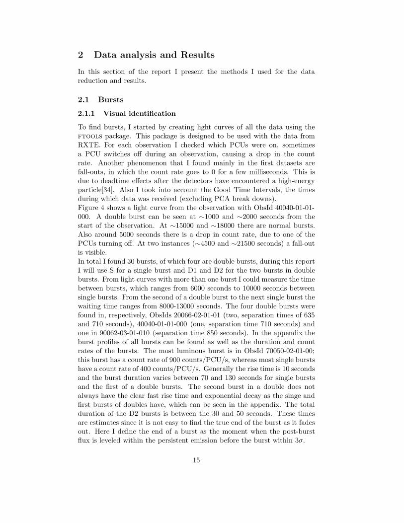
To find bursts, I started by creating light curves of all the data using theftools package. This package is designed to be used with the data fromRXTE. For each observation I checked which PCUs were on, sometimesa PCU switches off during an observation, causing a drop in the countrate. Another phenomenon that I found mainly in the first datasets arefall-outs, in which the count rate goes to 0 for a few milliseconds. This isdue to deadtime effects after the detectors have encountered a high-energyparticle[34]. Also I took into account the Good Time Intervals, the timesduring which data was received (excluding PCA break downs).Figure 4 shows a light curve from the observation with ObsId 40040-01-01-000. A double burst can be seen at ∼1000 and ∼2000 seconds from thestart of the observation. At ∼15000 and ∼18000 there are normal bursts.Also around 5000 seconds there is a drop in count rate, due to one of thePCUs turning off. At two instances (∼4500 and ∼21500 seconds) a fall-outis visible.In total I found 30 bursts, of which four are double bursts, during this reportI will use S for a single burst and D1 and D2 for the two bursts in doublebursts. From light curves with more than one burst I could measure the timebetween bursts, which ranges from 6000 seconds to 10000 seconds betweensingle bursts. From the second of a double burst to the next single burst thewaiting time ranges from 8000-13000 seconds. The four double bursts werefound in, respectively, ObsIds 20066-02-01-01 (two, separation times of 635and 710 seconds), 40040-01-01-000 (one, separation time 710 seconds) andone in 90062-03-01-010 (separation time 850 seconds). In the appendix theburst profiles of all bursts can be found as well as the duration and countrates of the bursts. The most luminous burst is in ObsId 70050-02-01-00;this burst has a count rate of 900 counts/PCU/s, whereas most single burstshave a count rate of 400 counts/PCU/s. Generally the rise time is 10 secondsand the burst duration varies between 70 and 130 seconds for single burstsand the first of a double bursts. The second burst in a double does notalways have the clear fast rise time and exponential decay as the singe andfirst bursts of doubles have, which can be seen in the appendix. The totalduration of the D2 bursts is between the 30 and 50 seconds. These timesare estimates since it is not easy to find the true end of the burst as it fadesout. Here I define the end of a burst as the moment when the post-burstflux is leveled within the persistent emission before the burst within 3σ.

15

Figure 4: The light curve of 4U 1323-62 from one of the observations in40040-01-01-000, with a time resolution of 1 second. In this light curvethere is a double burst visible (the first set) and two single bursts. Alsoaround 5000 seconds into the observation one of the PCUs turned off, whichis visible as a drop in the count rate. There are two detector drop-outs at∼3500 and ∼21500 seconds. Here the count rate is zero due to high energyparticles.

16

2.1.2 Spectral fitting

None of the bursts looked like PRE-burst in the light curves. To be sureI fitted the spectra of the bursts with a blackbody spectrum. PRE burstsshow characteristic behaviour in the spectra, the black-body temperaturedips simultaneously to a peak in the effective black-body radius. To modelthe bursts I used the xspec program.Using the light curve I find a rough estimate of the start and end points ofthe bursts. Then I extracted spectra from the burst every 0.5 seconds. Ialso made a spectrum of the persistent emission just before the burst. Thiscontains data from both the source and the background. The persistentemission is due to continued accretion during the burst, but since the burstis much more luminous I can safely subtract this emission to keep only theburst emission.Using both the burst spectra and the persistent spectra in xspec I candetermine the ’true’ start and stop of the burst. This is done by subtractingthe persistent emission from the burst emission. xspec gives the count rateand error of the persistent-level subtracted emission. If the count rate of thesubtracted spectrum is more than 3σ different from zero, the burst emissionis not leveled with the persistent emission. If in the count rate is less than 3σdifferent from zero, I assumed that the emission is leveled with the persistentemission.To know which channels correspond to which energy bands I need to create aresponse matrix. This is not only because the data can be binned in severalconfigurations, but also because the channel-energy relation changes overtime. The observed emission (O, per channel ch) is a convolution of theresponse matrix (R, depending on the energy E and the channel ch) andthe real emission (depending on energy E):

O(ch) =

∫

R(E, ch)I(E)dE (6)

Which can also be expressed as :−→O = R

−→I . The observed emission O and

the response matrix R are known. However, we cannot invert this equationinto R−1−→O =

−→I , this will create large errors. xspec will assume I ′ and will

create−→O′ = R

−→I ′ .

−→O′ will be compared to

−→O . If they are not the same I ′ will

be adapted and the process will be repeated until the difference |−→O′ −

−→O |2

is minimal. Then it can be assumed that−→I ′ =

−→I and the real emission is

known.Creating the response matrix can be done with the tool pcarsp. To usepcarsp one needs to provide a spectrum-file (.pha), an attitude file (neededif the satellite was not pointed directly at the source, not necessary in thiscase), the layers used (all) and the detectors used (all).In xspec I ignore the energies in the ranges 0-2.5 and 25+ since they arenot properly calibrated. The model I used for the fit is a simple absorption

17

model (wabs) to account for the interstellar absorption in the direction ofthe source, times a blackbody spectrum (bbody). The absorption modelaccounts for the photo-electric absorption the radiation undergoes on theway to the observer. This model has only one parameter, the equivalenthydrogen column N in units of 1022 atoms/cm2:

M(E) = exp(−Nσ(E)) (7)

The function σ(E) is the photo-electric cross-section and depends on theelement abundance in the interstellar medium. Here we assumed solar abun-dances. The blackbody spectrum models the radiation from the source itselfand has two parameters: the temperature kT (in keV) and a normalizationconstant K:

A(E) = 8.0525KE2dE

(kT )4(exp(E/kT ) − 1)(8)

Where K is defined as

K = (L39

d210

) (9)

Here L39 is the luminosity of the source in units of 1039 ergs/s and d10 isthe distance to the source in units of 10 kpc.Earlier measurements found the equivalent hydrogen column towards 4U1323-62 to be 4×1022 atoms/cm2 (Parmar et al., 1989 [20]. I ran the fit pro-gram twice, once with the equivalent hydrogen column fixed to that valueand once letting this parameter free. When calculating the errors for bothcases I estimate both the 68% and the 90% confidence levels. If given pa-rameter was not 3σ or more significant, I calculated the 95 % confidenceupper limit. In reality this applies for the equivalent hydrogen column NH

and the normalization parameter K. For the temperature parameter kT ,especially in the beginning of the burst, it is possible to get 68% confidencelevel parameter estimates. For an example of the fitted spectra see Figures5 and 6.After fitting all the spectra I used Matlab to produce plots of the param-

eters. In the appendix, Section D are the fits for all bursts. A PRE burstwould show a drop in temperature during the bursts. Also the normalizationof the blackbody component would go up since it is linked to the radius viathe luminosity. However, I was unable to find such a burst.

2.1.3 Distance determination

I was unable to find a PRE-burst and cannot determine the distance exactly.However, I am able to set an upper limit to the distance using the brightestburst: the second burst in 70050-03-01-00 which has a count rate of 900counts/s/PCU, more than twice the count rate of other bursts. We knowthis burst has a luminosity less then the Eddington limit. I calculate the

18

Figure 5: xspec plot of 4U 1323-62 of the first burst in 40040-01-01-000.This spectrum is taken 2 seconds after the burst has started and has anexposure of 0.5 seconds. The spectrum covers the 2.5-25.0 keV energy range.The fitted model is also plotted. The lower plot shows the residuals to thebest-fit model.

Figure 6: xspec plot of 4U 1323-62 of the first burst in 40040-01-01-000.This spectrum is taken when the burst is almost over, 88 seconds after theburst has started and has an exposure of 0.5 seconds. The spectrum coversthe 2.5-25.0 keV energy range. The fitted model is also plotted. The lowerplot shows the residuals to the best-fit model.

19

distance to the burst if it did have a luminosity at the peak of the burstequal to the Eddington luminosity to find the upper limit.

d =

√

LEdd

4πFpeak(10)

I set the luminosity equal to the Eddington limit: 3.7 ×1038 ergs/s(for a 1.4M⊙ neutron star, Kuulkers et al., 2003[30]), see section 1.3.2. I canuse the value of the normalization parameter K to find the flux:

K =L39

d210

=L

d2× 10−37 (11)

Here I can substitute for the luminosity:

K =4πσR2T 4

d2= 4πFbol (12)

Here Fbol is the bolometric luminosity. The value for K from the fit is(8.8±0.4)×10−2 , giving a 4πFbol of (8.75±0.4)×1035 ergs/s/kpc2. Now plug-ging this in the formula 10 with the Eddington Luminosity this gives an up-per limit to the distance (since the peak luminosity of the burst is in fact notequal to the Eddington luminosity but less) of 21.4±0.6 kpc. The error onlydepends on the error in K. The value found is consistent with the previousestimate of the distance being 10-20 kpc by Parmar et al (1989)[20].

2.2 Colour-colour and colour-intensity diagrams

To study the dipping in the source and to see the behaviour of the sourcein the colour-colour diagram I create light curves in different energy bands.For this I use the Std-2 data and a time resolution of 16 seconds. For eachobservation I produce five light curves: 2.0−3.7 keV, 3.7−6.1 keV, 6.1−9.7keV, 9.7 − 16.0 keV and 2.0 − 16.0 keV.After this I subtract the background in these bands. The background isestimated using the data from PCU 2 in the Std-2 files, because this PCU isalways on. In the Std-2 files the particle rates are included that are necessaryto estimate the background. During the creation of the background dead-time corrections are also taken into account. The background is estimated byusing matching background conditions to the observations to models whichcontain actual background observations.I define the soft and hard colour as respectively 3.7−6.1 keV/ 2.0−3.7 keVand 9.7 − 16.0 keV /6.1 − 9.7 keV count rate ratios in these bands. I definethe intensity as the entire 2.0 − 16.0 keV band count rate.

2.2.1 Hardness-diagrams and hardness-intensity diagrams

To study the dipping behaviour of the source I have made hardness-plots.Here I plot the hard colour versus time and compare it with the count rate

20

of all channels versus time. By comparing these plots the dips are easy torecognize, see for example Figure 10.The dipping properties differ between observations. For ObsId=20060 thehard colour during non-dips (persistent emission) is between 0.7 − 0.8 andduring dips this goes to 1− 1.3. The bursts have a hard colour of 0.55, alsoone burst that happens during a dip. For ObsId=40040, the hard colourfor the persistent emission is the same 0.7 − 0.8, but the dips have a hardcolour of 1.1− 1.65. Here the bursts have a hard colour of 0.55 as well, alsothe one burst that happens during a dip. For ObsId=70050 the hard colourduring the persistent phase is 0.5, which is a drop compared to the previousobservations. During dipping the hard colour ranges between 0.85 − 0.95and during bursts the hard colour is between 0.25 − 0.3. In ObsId=90062the hard colour returns to 0.7 − 0.8 for non-dipping intervals and 1.1 − 1.9during dipping. The hard colour during bursts is 0.45 and two bursts hap-pened during dipping.In total I have found 30 bursts, of which 6 happened during dipping inter-vals, including 1 of the 4 double bursts. Since the dipping lasts for 30% ofeach cycle, one would expect slightly more bursts (10) to happen during thedipping. The bursts that happen during a dip have a lower average countrate (293.7 counts/PCU/s including D2-bursts, 327.4 counts/PCU/s exclud-ing D2-bursts) than the average of all bursts (342.6 counts/PCU/s includingD2-bursts and the largest burst, 377.2 counts/PCU/s excluding D2-bursts,but including the largest burst and 356.4 counts/PCU/s excluding both theD2-bursts and the largest burst).For the hardness-intensity plots I use the hard colour as defined before andthe intensity in the total 2.0 − 16.0 keV-band. In Fig 7 I plot the sampleddata with error bars. In Fig 8 the shape of the data is more visible. HereI have also indicated where the different observations happen. As shown inthe plot, the observations are divided in ’streaks’ which have a left to rightmotion and bend slightly down towards the right. ObsId 20066, part ofObsId 40040 and ObsId 90062 are located in the middle streak. The rest ofObsId 40040 is visible in the high streak and ObsId 70050 is entirely in thelowest streak. I have plotted the dipping behaviour in Fig 9. As expectedthe dipping is visible in the higher left corner of each observation where theintensity is lower and the hard colour higher.

21

Figure 7: Hard colour versus intensity with error bars for all RXTE ob-servations of 4U 1323-62. Each dot represents data with a duration of 256seconds. The bursts have been removed from the data set and the coloursare normalized by Crab (see text for details).

0.8

1

1.2

1.4

1.6

1.8

2

0.003 0.004 0.005 0.006 0.007 0.008 0.009 0.01

Har

d co

lour

9.7

-16.

0/6.

0-9.

7 ke

V

Intensity 2.0-16.0 keV

Figure 8: Hard colour versus intensity of 4U 1323-62 per observation. Greencircles are data from ObsId=20060, blue crosses ObsId=40040, red plussesObsId=70050 and black stars ObsId=90062. Each dot represents data witha duration of 256 seconds.

3 4 5 6 7 8 9 10

x 10−3

0.8

0.9

1

1.1

1.2

1.3

1.4

1.5

1.6

1.7

1.8

Intensity 2.0−16.0 keV

Har

d co

lour

9.7

−16

.0/6

.0−

9.7

keV

22

Figure 9: Hard colour versus intensity of all data from the RXTE observa-tions of 4U 1323-62. The green points show the dipping phase, which is onthe higher left part of each streak, where the hard colour is higher and theoverall is intensity lower. Each dot represents data with a duration of 256seconds.

23

Figure 10: An example of a light curve of 4U 1323-62 combined with a plot of time versus the hard colour. This plot istaken from the observation 40040-01-03-000. This observation lasts for 2.5x104 seconds and shows 4 bursts and three episodesof dipping. The first burst takes place during the dip. The bursts are clearly seen as peaks in the lightcurve and a smalldownward excursion in the hard colour. The dips appear as irregular episodes in the lightcurve and as intervals of increasedhardness in the hardness versus time plot.

24

2.2.2 Colour-colour diagram

The colour-colour diagram was made twice. I first made a preliminary CCDusing the Std-2 data as described before. I removed the bursts and plottedthe soft against the hard colour. Figure 11 shows the plot. One would ex-pect to see an atoll or Z-shape, but the source traces no visible pattern, butrather random islands. This has several causes; the PCA has changed overtime and the channel-to-energy distribution and effective area have changedas well. The five PCU’s all behave differently. Also, initially, I did not in-terpolate in channel space to define fixed energy boundaries for each band.To correct for the gain changes and the differences in effective area, I nor-malize the colours and intensity of 4U 1323-62 by the corresponding Crabvalues, using observations that are close in time. The Crab Nebula has aconstant X-ray emission over time scales much longer than the spin periodof the Crab pulsar of ∼ 33 ms (Toor & Seward, 1974[42], van Straaten, vander Klis & Mendez (2003) [43]), making it a very useful source to calibrateX-ray instruments. See Fig E (in the appendix) for the evolution of softcolour (defined as 3.5 − 6.0/2.0 − 3.5 keV) of the Crab versus time. Visiblein the figure are the four gain changes, in which the PCU was reset to anew gain. To find the correct count rates in each energy band I interpolatedlinearly in channel space.

To make the final CCD I used corrected data. There is a slight changein the energy bands for this diagram compared to the previous one. Thecolours are now defined as soft and hard colour as 3.5 − 6.0 keV/ 2.0 − 3.5keV and 9.7 − 16.0 keV /6.0 − 9.7 keV, respectively. This CCD can be seenin Figure 13. Each point represents 256 seconds of data. Without the sam-pling the shape of the source is less visible due to hysteresis. However, stillthe source does not show a clear atoll or Z-shape. The first set of observa-tions (ObsId = 20066) was taken in 1997 during 4 consecutive days, and islocated in the middle of the CCD with an average hard colour of ∼1.35 andan average soft colour of ∼2. The next set (ObsId = 40040) was taken in1999 distributed over 3 months; the source started out in the middle of theCCD with average hard and soft colour similar to those in ObsId 20066, butduring the last observation in this set the source was in the upper right partof the CCD, with an average hard colour of ∼1.5 and an average soft colourof ∼3. The following set (ObsId = 70050) was taken in 2003 during oneday. The source was then at the lower left part of the CCD, with an averagehard colour of ∼1 and an average soft colour of ∼1.5. The last set (ObsId= 90026) was taken in 2004 during two consecutive days. The source wasback again in the middle of the CCD, with hard and soft colour similar tothose of the first two observations.One can use this CCD to study bursting and dipping behaviour, by connect-ing burst and dipping properties to the state of the source. Using the CCDI can track where the bursts happen and check if the bursting behaviour

25

Figure 11: First CCD of 4U 1323-62, of all RXTE data. Here background-subtracted Std-2 data is used. All points represent the average colours ineach separate observation. The hard colour is defined as 9.7 − 16.0 keV/6.1 − 9.7 keV and the soft colour as 3.7 − 6.1 keV/ 2.0 − 3.7 keV. For thisplot I have not corrected for the detector gain change and the change ineffective area of the detectors over the years. Green circles are data fromObsId=20060, blue crosses ObsId=40040, red pluses ObsId=70050 and blackstars ObsId=90062.

26

Figure 12: Second CCD of 4U 1323-62, using background subtracted Std-2 data that is corrected for detector gain changes and effective area andsampled every 256 seconds. The colours are defined slightly different thanbefore: hard colour is defined as 9.7 − 16.0 keV /6.0 − 9.7 keV and the softcolour as 3.5 − 6.0 keV/ 2.0 − 3.5 keV.

0.8

1

1.2

1.4

1.6

1.8

2

1 1.5 2 2.5 3 3.5 4

Har

d co

lour

9.7

-16.

0/6.

0-9.

7 ke

V

Soft colour 6.0-3.5/2.0-3.5 keV

Figure 13: The CCD of 4U 1323-62. Same data as in Fig 12 but withindication of the observations. Color coding is the same as for Figure 11;green circles are data from ObsId=20060, blue crosses ObsId=40040, redpluses ObsId=70050 and black stars ObsId=90062. (Error bars left out forclarity, see Fig 12)

1 1.5 2 2.5 3 3.5 40.8

0.9

1

1.1

1.2

1.3

1.4

1.5

1.6

1.7

1.8

Har

d co

lour

9.7

−16

.0/6

.0−

9.7

keV

Soft colour 3.5−6.0/2.0−3.5

27

Figure 14: The CCD of 4U 1323-62, each point representing 256 seconds ofdata, where the moment before the burst is indicated. The blue points showwhere a single burst happens and the green points where a double bursthappens. The black dot indicates the brightest burst.

can be related to the state of the source. Figure 14 shows the CCD witherror bars again, with an indication of the point before a burst happens. Inthis Figure also the most luminous burst is indicated with a black dot. Thisburst is the left most burst in the entire plot, but not the softest. I havealso indicated the dipping behaviour in Figure 15. The dipping periods arelocated at the top-right part of each observation “isle” but is connected toit. The dips do not all happen in the same place of the CCD nor are theycompletely disconnected from the non-dipping state.

2.3 Timing analysis

I make the power spectra using the fft xte routine, which takes the FITSfiles and produces a .tra file. fft xte reads metafiles, where the observa-tions are listed in the metafile. The observations are then put in chronologi-cal order and the first point is determined, t0. After this the user is asked toselect the energy channels for the analysis and to give the time resolution τ .Using the fact that these systems have never shown variability above 2000Hz I set the Nyquist frequency, νNy at 2048 Hz, a power of 2.

τ =1

2νNy(13)

28

Figure 15: The CCD of 4U 1323-62, each point representing 256 seconds ofdata, where the dipping events are indicated by green crosses. During thedipping the source becomes harder. The dipping events are not completelydisconnected from the non-dipping ’isles’.

0.7

0.8

0.9

1

1.1

1.2

1.3

1.4

1.5

1.6

1.7

1.8

1 1.5 2 2.5 3 3.5 4

Har

d co

lour

9.7

-16.

0/6.

0-9.

7 ke

V

Soft colour 6.0-3.5/2.0-3.5 keV

The Good Xenon files have a time resolution of 0.95 µs, so I need to rebinthe data by a factor 256 to get the wanted resolution. For the Event filesthe time resolution is 125 µs which needs to be rebinned only twice. I chosethe length of the FFT, LFFT , to 16 seconds and averaged the 16-s powerspectra within each observation to reduce noise contributions. The length ofthe intervals, LFFT , determines the lowest frequency reached in the powerspectrum, which is 1/LFFT . So with a length of 16 seconds it is possibleto reach a minimum frequency of ∼0.1 Hz. Observations that were close intime were processed together to improve the statistics.After this I use the Clean tra routine to remove bursts. During a burst thepersistent emission from the source is overshadowed by the burst emission.To further study the power spectra I use the xana routine, that reads thepower spectra. Before I can analyse the spectrum I need to subtract thePoisonnian noise. This noise is due to the random nature of the arrivalof photons in the time series. The power spectrum of a Poisson process,when properly normalized (Leahy, 1983 [47]), follows a χ2-distribution with 2degrees of freedom. Hence, the expected average power is 2, and the varianceis 4. Because of the averaging of the power spectra of consecutive segmentsof 16 second duration, the variance of the Poissonian noise is actually 4/Nwhere N is the number of averaged power spectra. Due to dead-time effectsthe noise level can be above or below 2. This source is not very bright sothe dead-time effects are not that important for this.

29

To subtract this Poisson level of the power spectrum I take the very lastpart of the power spectrum, from 1500 Hz to the end. Since I suppose thereis only noise here, I fit this with a straight line. I subtract this amount fromall bins. In Figure 16 the difference between the raw and Poisson-subtractedpower spectrum is shown.

Figure 16: Power spectra of ObsId 20066-02-01-03. The left panel showsthe raw power spectrum, where the power from about 10 Hz seems to be2. The right panel shows the power spectrum where the Poissonian noise issubtracted. Visible in this spectrum is the 1-Hz QPO.

Raw spectrum Poisson-subtracted spectrum

2.3.1 Discovery of a kilohertz QPO

After this I fit the power spectra with a power law and 3 Lorentzians whichgives the best fit, except for the observations with ObsId=70050. The fitsfor all observations are shown in the appendix.For ObsId=70050 I combined the observations 70050-03-01-00 and 70050-03-01-02 which are very close in time (with a gap of 1408s) and fitted themwith three Lorentzians only. The results can be found in Table 1 and Figure17. I could not get a good fit of 70050-03-01-01 since it has a low signal tonoise ratio (S/N).In Figure 17 the Lorentzians have central frequencies of 0.3, 15.8 and 503.0

Hz. I do not detect the 1-Hz QPO in this observation with 95% confidenceupper limit of 7.1 % rms amplitude. However, I found the Lorentzian at 503Hz to be significant with a 7.1σ single trial significance; the significance wascalculated by comparing the power of the Lorentzian to the power of thepoissonian background < P >, which is defined as < P >= 2± 2√

NW, where

N is the number of power spectra and W is the number of frequencies thatI averaged in the power spectrum. The rms amplitude of the 503-Hz QPO

30

Figure 17: A 3-Lorentzian fit to the combined power spectrum of observa-tions 70050-03-01-00 and 70050-03-01-02, the Poisson-levels have been sub-tracted as described in the text. The parameters for the fit can be foundin Table 1. The red line is a Lorentzian with a central frequency of 0.34Hand the green line has a central frequency of 15.8 Hz. The blue line has acentral frequency of 503 Hz and fits the kHz QPO.

31

Table 1: Results of the fit of 70050-03-01-00 and 70050-03-01-02 combinedusing 3 Lorentzians. χ2 = 42.6/31Lorentzian Central frequency Rms amplitude FWHM

1 0.34 ± 0.09 Hz 4.9 ± 1.2 % 0.4 ± 0.32 15.8 ± 0.8 Hz 13.1 ± 1.8 % 10.0 ± 2.53 503.0± 40.2 Hz 36.6 ± 4.2 % 398.4 ± 142.3

Table 2: Results of the fit of 70050-03-01-00 and 70050-03-01-02 combinedin the energy ranges 0-4 keV and 4-30 keV with the 68% confidence leveland 95% upperlimit (UL).Energy range All parameters free ν, FWHM fixed ν, FWHM fixed

Using the full energy fit Using the best fit

0-4 keV rms (68%) 97.9%±35.0% 34.0%±33.9% 98.0%±14.90-4 keV rms (95% UL) 81.7 % 116.7%

4-30 keV rms (68%) 18.8%±6.3% 18.8%±6.3% 18.8%±4.6%4-30 keV rms (95% UL) 27.9% 24.5%

is 36.6 ± 4.7 % and the FWHM is 398 ± 142.3 Hz.I divided the spectra into two energy bands: 0-4 keV and 4-30 keV, createdpower spectra of each band and in each band tried to fit Lorentzians tothe feature and measure the rms energy spectrum of this QPO. I first triedhaving all model parameters free. However, I was unable to get significantresults, due to the low count rate. After this I fixed the frequency andFWHM to the best-fit values of the full-band spectrum and left only thepower free. This is done twice with the parameters from the best fit of thetotal energy spectrum (here I assume that the frequency and FWHM areenergy independent) and the parameters of the best fit of the specific energyspectrum (which were consistent with the values obtained from the fits tothe full energy band). The results are given in table 2. I did not detect asecond QPO, even though kHz QPOs tend to appear in pairs (Mendez &Belloni, 2007 [39]).

2.3.2 Hysteresis

Since I wanted to study the path of the source in the colour-colour diagramI want to see if the source might be showing hysteresis: this occurs when thesource is at the same point several times while following a different path toreach that point each time. I compared the integrated power in the powerspectra within a fixed frequency range with the frequency of the QPO at1 Hz. To measure the 1-Hz QPO I fit the power spectrum from 0.1 Hz to100 Hz with a power law and one Lorenzian. The results can be found in

32

Table 8. As mentioned before I did not detect the 1-Hz QPO in the datasets70050-03-01-00 and 70050-03-01-01. The spectrum of 70050-03-01-01 wasdifficult to fit since it has a low S/N. In the sets 40040-01-01-000 and 40040-01-03-000 we found a QPO at 1.9 Hz and 2.6 Hz, respectively. Since thesevalues are about twice as high as the values found in the other observationswith 1-Hz QPOs, we argue that in these observations we have detected har-monics of the 1-Hz QPO. I found a second significant (3.1-σ) Lorentzian in40040-01-01-000 at 0.98 Hz, which has less power than the Lorentzian at1.86 Hz. For 40040-01-03-000 I was unable to find a significant Lorentzianat half the frequency of the 2.6-Hz QPO, but we found a likely one at afrequency of 1.2 Hz with a 2.7 σ significance.To find the rms in a fixed frequency range I added the power in each fre-quency bin between 0.1 and 100 Hz after subtracting the Poisson level. Thispower is converted into rms amplitude and is plotted versus observationnumber together with the frequency of the 1-Hz QPO in Figure 18, wherethe observations are sorted in time. In this figure the 0.1-100 Hz integratedpower is steady around 25 % rms amplitude for the ObsId=20066 (averagerms power is 25.5%) and 40040 (average rms power is 24.8%), where forObsId=40040-01-03-000, the observation that is at the right most positionin the CCD, is slightly lower at 22 %. After this, the power drops to ∼10%for ObsId=70050-03-01-00 (the left most point in the CCD), the averagerms power for ObsId=70050 is 15.6%. The rms power then increases to ∼26% for ObsId=90026, where the average is 26.5%. The average frequency ofthe 1-Hz QPO is 0.83 Hz for ObsId=20066. In ObsId=40040 the averageis 0.63 Hz if the uncertain points and subharmonics are not taken into ac-count. If I do take the subharmonics into account the average is 1.4 Hz.For ObsId=70050 there is no 1-Hz QPO. In the last set, ObsId=90062, thefrequency is 0.81 Hz on average.The observations with ObsId=20066, part of ObsId=40040 and ObsId=90062have overlapping points in the CCD. If the source is in the same state thiswould mean the average power and the frequency of the 1-Hz QPO wouldbe similar. Using the above measurements I can say that ObsId=20066 andObsId=90062 are indeed similar states. The power spectra of these observa-tions are also very similar (see Appendix). Even though the average powerof the observations with ObsId=40040 are similar to the observations in Ob-sId=20066 and ObsId=90062, one can clearly see that in the observationsin ObsId=40040 the source is in a different state. Not only in the frequencyof the 1-Hz QPO but also in the appearance of (sub) harmonics instead ofone clear peak. For ObsId=70050 the source is clearly in a different statethan the rest of the observations. Not only is the 1-Hz QPO not visible, theaverage power is very weak compared to the other states.I can conclude that the source indeed shows hysteresis, which, together withthe time sampling of observations, may cause the strange shape of the CCDof this source.

33

Figure 18: Evolution of the frequency (black circles with error bars) of the1-Hz QPO and the broad-band rms amplitude (between 0.1 to 100 Hz, greendashed line) plotted versus the ObsId. The observations are ordered in time.For two observations, 40040-01-01-000 and 40040-01-03-000 (points 6 and 9in the plot), I have probably observed an harmonic since the frequency ofthe peak is about twice as high as the previous and next observations. For40040-01-01-000 I was able to fit a significant Lorentzian to the expectedfrequency of the QPO based on the harmonic (star) For 40040-01-03-000 Icould not find a significant Lorentzian. In this case I have plotted a pointfor the likely QPO frequency based on the harmonic (blue square). Theorder of the observations: 20066-02-01-00, 20066-02-01-03, 20066-02-01-01,20066-02-01-04, 20066-02-01-02, 40040-01-01-000, 40040-01-02-000, 40040-01-02-01, 40040-01-03-000, 70050-03-01-01, 70050-03-01-00, 70050-03-01-02,90062-03-01-00, 90062-03-01-02, 90062-03-01-010.

1 2 3 4 5 6 7 8 9 10 11 12 13 14 15 160

1

2

3

Fre

quen

cy o

f the

1−

Hz

QP

O

1 2 3 4 5 6 7 8 9 10 11 12 13 14 15 160

5

10

15

20

25

30

RM

S a

mpl

itude

from

0.1

Hz

to 1

00 H

z

Observations in chronological order, see caption

34

3 Discussion

I have analysed the full set of RXTE observations of the neutron-star low-mass X-ray binary 4U 1323-62. For this thesis I carried out both spectraland timing analysis of the observations. I will now discuss my results.

3.1 Calculation of the distance

I have tried to constrain the distance to the neutron-star low-mass X-raybinary 4U 1323-62 using photospheric radius expansion bursts. Being unableto find such a burst, I used the brightest burst in my sample to find anupper limit to the source distance of 21.4±0.6 kpc. To find this value Imade some assumptions: the mass of the star, the chemical compositionand the anisotropy of the burst emission. The possible mass of neutronstars range from 0.1 M⊙ to 3 M⊙, with mass distribution peaks at 1.27M⊙and 1.76M⊙ for Type II supernovae and 1.31 M⊙ for type 1b supernovae(Timmes, Woosley & Weaver, 1996 [48]). Without making assumptions ofthe progenitor event that formed the neutron star, I have assumed a massof 1.4M⊙, which fits with both ranges. The chemical compostion rangesbetween X=0 for hydrogen poor material to X=0.7 for cosmic abundances.Here I have used X=0, based on Kuulkers et al., 2003 [30], who foundthat the hydrogen-poor composition better fitted the distance measurementsto 12 sources with a known distance. We did not take into account theanisotropy of the burst emission. However, since 4U 1323-62 has a highinclination the emission from the source is not expected to be isotropic(Boirin et al, 2007 [21]).

3.2 Colour analysis

Using colour-colour and hardness-intensity diagrams I have characterisedthe behaviour of the source in detail. I have correlated the bursting be-haviour of the source with the states in the CCD (Figure 14). The doublebursts happen in the middle of the CCD and the most luminous burst hap-pens when the source is in the leftmost state. If the source would trace anatoll-like shape, the left most part of the CCD corresponds to the state inwhich the mass accretion rate is highest among these observations. This canexplain the very bright burst at this point. The bursts in this state are alsoshorter than those in other states (71.3 seconds compared to 119.9 secondsin the middle state). This is in agreement with the notion that if the massaccretion rate increases the amount of hydrogen in the burning material ofthe burst decreases (which causes shorter bursts [2]).The double bursts only happen in the middle part of the CCD. Double (alsotriple and quadruple) bursts are linked to mixed hydrogen/helium burning,which is thought to happen at low accretion rates (Galloway et al., 2008

35

[32]).When the source is in the right most part of the CCD, there are no doublebursts, and the bursts that happen in this state have slightly shorter dura-tions than average (101.3 seconds compared to 119.9 seconds), which wouldpoint to higher accretion rates than the observations in the middle state ofthe CCD.

3.3 Timing analysis

I have discovered a kilo-hertz quasi-periodic oscillation, with a frequency of503 Hz in this source. The kHz QPO is only detected in observations Ob-sId=70050 and not in the other observations, with 95 % upper limits givenin Table 7. This is the third high-inclination source in which a kHz QPOis discovered, the other sources are 4U 1915-05 (Barret et al., 1997[46] andEXO 0748-676 (Homan & van der Klis, 2000 [45]). Since kHz QPOs aresupposed to originate at the inner regions of the accretion disc, one wouldnot expect to see them in high inclination systems, where the inner disc isocculted by the outer parts of the disc. This suggests that, although thekHz QPO could be produced close to the neutron star, a mechanism relatedto an extended component (eg. the corona) is needed to make the kHz QPOvisible. This is consistent with previous results (Berger et al., 1996 [49])that show that the spectrum of the emission responsible for the QPOs is toohard to be attributed to the accretion disc.Also it is interesting that the 1-Hz QPO is detected in all our observationsexcept in the one where I detected the kHz QPO. This is also the case forEXO 0748-676 (Homan & van der Klis, 2000 [45]). Furthermore the appear-ance of the kHz QPO and the disappearance of the 1-Hz QPO happens inthe left most state of the CCD. It might be that the 1-Hz and the kHz QPOsare connected, and that there is a physical change in the accretion disc thatfavors the production of either one or the other.

4 Conclusions

In this research I have studied the Low-mass X-ray binary source 4U 1323-62. I have used thermonuclear X-ray bursts to set an upper limit to thedistance using the theory of photospheric radius expansion bursts, assuminga neutron star mass of 1.4M⊙, hydrogen poor material and isotropic emis-sion. The calculated upper limit to the distance to 4U 1323-62 I found is21.4±0.6 kpc, which is consistent with earlier constraints to the distance of10-20 kpc (Parmar et al., 1989 [20]).I have also studied the dipping of the source by looking at the time evolutionof the hard colour of the source combined with light curves. I have further in-vestigated the connection between the persistent non-dipping phase and the

36

dipping phase by studying hardness-intensity diagrams (HIDs) and colour-colour diagrams (CCDs). During the dipping phase the source spectrum isharder, and luminosity decreases compared to the the non-dipping phase,but that the two phases are not so different they appear as different states ineither the HID or the CCD. The colour-colour diagram of the source showsneither a clear atoll nor Z-shape. This is probably caused by bad sampling,the data has been taken with long (more than weeks) intervals and generallylast for one day, and hysteresis, the source moves through the same point inthe CCD but traces a different path.I have also studied the variability of the source using Fourier power densityspectra. I have detected a 7.1-σ significant kHz quasi-periodic oscillation(QPO) at 503±40.2 Hz. This is the first time a kHz QPO has been detectedin 4U 1323-62 and only the third time a kHz QPO is detected in a highinclination source (for the other sources see: Barret et al., 1997[46], Homan& van der Klis, 2000 [45]). I have connected the behaviour of the known1-Hz QPO to the newly discovered kHz QPO. In our observations, only oneis visible each time; if the 1-Hz QPO is visible, the kHz QPO is not and theother way around. Furthermore I have studied the behaviour of the 1-HzQPO and connected this to the power in a fixed frequency range to findwhether the source shows hysteresis. Using the data available I concludethat the source indeed shows hysteresis; it moves through the middle statewhile following (at least) two different paths.

References

[1] Various authors, ”X-ray binaries”, Cambridge Astrophysical Series, No26, 1995

[2] Various authors, ”Compact Stellar X-ray sources”,Cambridge Astro-phycial Series, No 39, 2006

[3] E.E. Salpeter, ApJ 140:796-800 (1964)

[4] I.S. Shklovsky, ApJ 148:L1-L4 (1967)

[5] J.E. Pringle, AR&A 19:137-162 (1981)

[6] W. Forman, C. Jones, L. Cominsky, P. Julien, S. Murray, G. Peters, H.Tananbaum & R. Giacconi, ApJS, 38: 357-412 (1978)

[7] R. S. N. Warwick et al., MNRAS, 197: 865-891 (1981)

[8] M. van der Klis, J. van Paradijs, F.A. Jansen & W.H.G.Lewin, 1984,IAU Circ. 3961

[9] M. van der Klis, A.N. Parmar,J. van Paradijs, F.A. Jansen, & W.H.G.Lewin, 1985b, IAU Circ. 4044

37

[10] M. van der Klis, ARA&A, 27:517:53 (1989)

[11] M. van der Klis, G. Hasinger, E. Damen, W. Penninx, J. van Paradijs& W.G.H. Lewin, ApJ 360:L19-L22, 1990 September

[12] M. van der Klis, AN 326,9: p.798-803 (2005)

[13] J. van Paradijs, W. Penninx & W.H.G. Lewin, MNRAS 233:437-450(1988)

[14] C. Done, M. Gierlinski & A. Kubota, A&AR, 15,1:1-66 (2007)

[15] K. Mitsuda, H. Inoue, K. Koyama, K. Makishima, M. Matsuoka, Y.Ogawara, N. Shibazaki, K. Suzuki & Y. Tanaka, PASJ 36:741-759(1984)

[16] P.G. Jonker, M. van der Klis, R. Wijnands, ApJ 511:L41-L44, 1999January 20

[17] A. Paizis et al., A&A 459:187-197 (2006)

[18] Y. Ko & T.R. Kallman, ApJ 431:273-301, 1994 August 10

[19] G.W. Clark,J.W. Woo, F. Nagase, K. Makishima & T. Sakao, ApJ,353:274-280, April 10 1990

[20] A .N. Parmar, M. Gottwald, M. van der Klis & J. van Paradijs, ApJ338:1024-1032, 1989 March 15

[21] L. Boirin, L. Keek, M. Mendez, A. Cumming, J.J.M. in ’t Zand, J.Cottam, F. Paerels & W.H.G. Lewin, A&A 465, 559-673, April 2007

[22] N.E. White & J.H. Swank, ApJ 253:L61-L66, 1982 February 15

[23] P.F. Bloser, J.E. Grindlay, D. Barret & L. Boirin, ApJ 542:989-999,2000 October 20

[24] S. Balman, ApJ, 138:50-62, 2009 July

[25] D.S. Balsara, J.L. Fisker, P. Godon & E.M. Sion, ApJ 702,2:1536-1552(2009)

[26] J.E. Gunn & J.P. Ostriker, ApJ 160:979-1002 (1970)

[27] J. Frank, A.R. King & J-P Lasota, A&A 178, 137-142(1987)

[28] K. Jahoda et al., ApJ Supplement series 163:401-423, 2006 April

[29] A. Heger, A. Cumming, D.K. Galloway & S. E. Woosley, ApJ671:L141L144, 2007 December 20

38

[30] E. Kuulkers, P.R. den Hartog, J.J.M. van ’t Zand, F.W.M. Verbunt,W.E. Harris & M. Cocchi, A&A 339:663-680 (2003)

[31] M. Ba lucinska-Church, M.J. Church, T. Oosterbroek, A. Segreto, R.Morley & A.N. Parmar, A&A 349:495-504 (1999)

[32] D.K. Galloway, M.P. Muno, J.M. Hartman, D. Psaltis & D.Chakrabarty, ApJSS 179:360-422, 2008 December

[33] G. Hasinger & M. van der Klis, A&A 225:79-96 (1989)

[34] T. A. Jones, A. M. Levine, E. H. Morgan & S. Rappaport, ApJ 677Issue 2:1241-1247 (2008)

[35] N.S. Schultz, G. Hasinger & J. Trumper, A&A, 225, 48-68 (1989)

[36] M. Kaufmann Bernado & M. Massi, Mem. S.A. It. Vol. 78, 393 (2007)

[37] L. Keek, D.K. Galloway, J.J.M. in ’t Zand & A. Heger, ApJ 718:292-305, 2010 July 20

[38] M. Mendez, M. van der Klis, E.C. Ford, R. Wijnands & J. van Paradijs,ApJ, 511:L49L52, 1999 January 20

[39] M. Mendez & T. Belloni, MNRAS 381:790-796 (2007)

[40] M.P. Muno, R.A. Remillard & D. Chakrabarty, ApJ 568:L35-L39, 2002March 20

[41] D. Psaltis, T. Belloni & M. van der Klis, ApJ 520:262-270, 1999 July20

[42] A. Toor & F.D. Seward, ApJ, 79:995-999 (1974)

[43] S. van Straaten, M. van der Klis & M. Mendez, ApJ 596:1155-1176,2003 October 20

[44] M.Y. Fujimoto & R.E. Taam, ApJ 305:246-250, 1986 June 1

[45] J. Homan and M. van der Klis, ApJ 539:847-850, 2000 August 20

[46] D.Barret, J.F. Olive, L. Boirin, J.E. Grindlay, P.F. Bloser, Y. Chou,J.H. Swank, & A.P. Smale, IAU Circ. 6793, 1997

[47] D.A. Leahy, W. Darbro, R.F. Elsner, M.C. Weisskopf, S. Kahn, P.G.Sutherland & J.E. Grindlay, ApJ 266:160-170, March 1983

[48] F.X. Timmes, S.E. Woosley & T.A. Weaer, ApJ 457:834-843, 1996February 1

[49] M. Berger et al., ApJL 496:L13-L17 (1996)

39

A Data

Table 3: A list of all data usedObservation name Observation date Time observed (sec) Time resolution

20066-02-01-00 25-26/4/1997 21200 0.95 µs20066-02-01-03 26/4/1997 11400 0.95 µs20066-02-01-01 26-27/4/1997 19600 0.95 µs20066-02-01-04 27/4/1997 11300 0.95 µs20066-02-01-02 27-28/4/1997 15500 0.95 µs40040-01-01-000 18/1/1999 27500 0.95 µs40040-01-02-000 23/2/1999 16400 0.95 µs40040-01-02-01 23/2/1999 8300 0.95 µs40040-01-03-000 13/3/1999 28900 0.95 µs70050-03-01-01 25/9/2003 9900 125 µs70050-03-01-00 25/9/2003 26500 125 µs70050-03-01-02 25/9/2003 10000 125 µs90062-03-01-00 12/30/2004 5950 125 µs90062-03-01-02 12/31/2004 4680 125 µs90062-03-01-010 12/31/2004 33600 125 µs

40

B Burst properties: profiles

The next figures show the profils of all X-ray bursts observed from 4U 1323-62 with RXTE. The burst profiles are plotted with a time resolution of 1second in a time frame of 250 seconds. On the x-axis is I plot the time, andon the y-axis the count rate. In total 30 bursts were found, eight of whichwere part of a double burst; consisting of a strong burst and a weaker burstfollowing within a short time interval.

Table 4: Burst profiles per dataset

Observation number: 20066-02-01-00

Observation number: 20066-02-01-01

41

Observation number: 20066-02-01-02 Observation number: 20066-02-01-03

Observation number: 20066-02-01-04

Observation number: 40040-01-01-000

42

Observation number: 40040-01-02-000

Observation number: 40040-01-02-01

43

Observation number: 40040-01-03-000

Observation number: 70050-03-01-00

44

Observation number: 70050-03-01-01 Observation number: 70050-03-01-02

Observation number: 90062-03-01-00

Observation number: 90062-03-01-010

45

Observation number: 90062-03-01-02

46

C Burst properties: duration and peaks

Table 5: The properties of the bursts per observation. The total durationis the time from the rise until the point where the burst emission is equalto the persistent emission. D1 and D2 are the first and second member ofdouble bursts, S are single bursts.Observation Type Duration to peak Duration total Count rate /PCU/s

20066-02-01-00 S 10 s 120 s 380S 10 s 110 s 370

20066-02-01-01 D1 9 s 130 s 348D2 5 s 50 s 78D1 9 s 125 s 340D2 10 s 50 s 126

20066-02-01-02 S 10 s 130 s 38020066-02-01-03 S 10 s 105 s 34020066-02-01-04 S 12 s 125 s 36040040-01-01-000 D1 6 s 110 s 380

D2 5 s 30 s 144S 10 s 125 s 350S 6 s 110 s 300

40040-01-02-000 S 10 s 120 s 305S 10 s 115 s 235

40040-01-02-01 S 8 s 155 s 23240040-01-03-000 S 7 s 90 s 382

S 11 s 100 s 337S 10 s 100 s 305S 10 s 115 s 362

70050-03-01-00 S 6 s 70 s 400S 6 s 70 s 900

70050-03-01-01 S 10 s 75 s 30070050-03-01-02 S 10 s 70 s 50090062-03-01-00 S 10 s 110 s 36090062-03-01-010 D1 10 s 130 s 385

D2 6 s 35 s 125S 10 s 102 s 500S 10 s 115 s 435

90062-03-01-02 S 10 s 122 s 320

47

D Burst fits

All bursts are fitted are fitted twice using xspec using an absorption modeland a black body model (for a detailed describtion see Section 2.1.2). Here Ishow all the fitted burst profiles. Where the equivalent hydrogen column,NH ,is free, the upper panel shows the count rate during the burst, the secondpanel the equivalent hydrogen column, the middle panel the keV evolution,the fourth panel the normalization constant of the blackbody and the lowestpanel shows the evolution of χ2. If the equivalent hydrogen column is fixed,at 4 × 1022 atoms/cm2 (see Section 2.1.2) the upper panel shows the countrate, the second keV , the third the normalization parameter and the lowestpanels shows the χ2 of each fit.

48

20066-02-01-00 Burst 1

Equivalent Hydrogen Column NH free

Equivalent Hydrogen Column NH fixed at 4 × 1022 atoms/cm2

0 10 20 30 40 50 60 70 80 900

500

1000

1500

2000Burst

Rat

e

0 10 20 30 40 50 60 70 80 900

1

2

3kT

keV

0 10 20 30 40 50 60 70 80 900

0.02

0.04

0.06Norm

0 10 20 30 40 50 60 70 80 900

0.5

1

1.5

2Chi2

Time, offset = 104629931.84

49

20066-02-01-00 Burst 2

Equivalent Hydrogen Column NH free

Equivalent Hydrogen Column NH fixed at 4 × 1022 atoms/cm2

0 10 20 30 40 50 60 70 80 90 1000

500

1000

1500

2000Burst

Rat

e

0 10 20 30 40 50 60 70 80 90 1000

1

2

3kT

keV

0 10 20 30 40 50 60 70 80 90 1000

0.02

0.04

0.06Norm

0 10 20 30 40 50 60 70 80 90 1000

0.5

1

1.5

2Chi2

Time, offset = 104638763.4

50

20066-02-01-01 Burst 1

Equivalent Hydrogen Column NH free

0 20 40 60 80 100 1200

1000

2000Burst

Rat

e

0 20 40 60 80 100 1200

10

20

30nH

102 2

atom

s/cm

2

0 20 40 60 80 100 1200

1

2

3kT

keV

0 20 40 60 80 100 1200

0.02

0.04

0.06

Norm

0 20 40 60 80 100 1200

1

2Chi2

Time, offset=104713140.4

Equivalent Hydrogen Column NH fixed at 4 × 1022 atoms/cm2

0 20 40 60 80 100 1200

500

1000

1500

2000Burst

Rat

e

0 20 40 60 80 100 1200

1

2

3kT

keV

0 20 40 60 80 100 1200

0.02

0.04

0.06Norm

0 20 40 60 80 100 1200

0.5

1

1.5

2Chi2

Time, offset = 104713140.4

51

20066-02-01-01 Burst 2

Equivalent Hydrogen Column NH free

0 5 10 15 20 25 300

200

400

Burst

Rat

e

0 5 10 15 20 25 300

20

40

nH10

( 22)

atom

s/cm

2

0 5 10 15 20 25 300

1

2

3kT

keV

0 5 10 15 20 25 300

0.05

0.1Norm

0 5 10 15 20 25 300

1

2Chi2

Time, offset=104713776.9

Equivalent Hydrogen Column NH fixed at 4 × 1022 atoms/cm2

0 5 10 15 20 25 300

100

200

300

400

Burst

Rat

e

0 5 10 15 20 25 300

1

2

3kT

keV

0 5 10 15 20 25 300

1

2

3

4

5x 10

−3 Norm

0 5 10 15 20 25 300

0.5

1

1.5

2Chi2

Time, offset = 104713776.9

52

20066-02-01-01 Burst 3

Equivalent Hydrogen Column NH free

0 20 40 60 80 100 1200

1000

2000Burst

Rat

e

0 20 40 60 80 100 1200

10

20

30nH

102 2

atom

s/cm

2

0 20 40 60 80 100 1200

1

2

3kT

keV

0 20 40 60 80 100 1200

0.02

0.04

0.06Norm

0 20 40 60 80 100 1200

1

2Chi2

Time, offset=104722468.9

Equivalent Hydrogen Column NH fixed at 4 × 1022 atoms/cm2

0 20 40 60 80 100 1200

500

1000

1500

2000Burst

Rat

e

0 20 40 60 80 100 1200

1

2

3kT

keV

0 20 40 60 80 100 1200

0.02

0.04

Norm

0 20 40 60 80 100 1200

0.5

1

1.5

2Chi2

Time, offset = 104722468.9

53

20066-02-01-01 Burst 4

Equivalent Hydrogen Column NH free

0 5 10 15 20 25 30 35 400

500

1000Burst

Rat

e

0 5 10 15 20 25 30 35 400

20

40

nH10

2 2 at

oms/

cm2

0 5 10 15 20 25 30 35 400

1

2

3kT

keV

0 5 10 15 20 25 30 35 400

0.02

0.04

0.06Norm

0 5 10 15 20 25 30 35 400

1

2Chi2

Time, offset=104723177.9

Equivalent Hydrogen Column NH fixed at 4 × 1022 atoms/cm2

0 5 10 15 20 25 30 35 400

500

1000Burst

Rat

e

0 5 10 15 20 25 30 35 400

1

2

3kT

keV

0 5 10 15 20 25 30 35 400

0.005

0.01Norm

0 5 10 15 20 25 30 35 400

0.5

1

1.5

2Chi2

Time, offset = 104723177.9

54

20066-02-01-02 Burst 1

Equivalent Hydrogen Column NH free

0 20 40 60 80 100 120 1400

1000

2000

Burst

Rat

e

0 20 40 60 80 100 120 1400

10

20

30nH

10e2

2 at

oms/

cm2

0 20 40 60 80 100 120 1400

1

2

3kT

keV

0 20 40 60 80 100 120 1400

0.02

0.04

0.06

Norm

0 20 40 60 80 100 120 1400

1

2Chi2

Time, offset=104809635.4

Equivalent Hydrogen Column NH fixed at 4 × 1022 atoms/cm2

0 20 40 60 80 100 120 1400

500

1000

1500

2000

2500Burst

Rat

e

0 20 40 60 80 100 120 1400

1

2

3kT

keV

0 20 40 60 80 100 120 1400

0.02

0.04

0.06Norm

0 20 40 60 80 100 120 1400

0.5

1

1.5

2Chi2

Time, offset = 104809635.4

55

20066-02-01-03 Burst 1

Equivalent Hydrogen Column NH free

0 20 40 60 80 100 1200

1000

2000

Burst

Rat

e

0 20 40 60 80 100 1200

10

20

30nH

10e2

2 at

oms/

cm2

0 20 40 60 80 100 1200

1

2

3kT

keV

0 20 40 60 80 100 1200

0.02

0.04

0.06

Norm

0 20 40 60 80 100 1200

1

2Chi2

Time, offset=104656901.9

Equivalent Hydrogen Column NH fixed at 4 × 1022 atoms/cm2

0 20 40 60 80 100 1200

500

1000

1500

2000

Burst

Rat

e

0 20 40 60 80 100 1200

1

2

3kT

keV

0 20 40 60 80 100 1200

0.02

0.04

0.06Norm

0 20 40 60 80 100 1200

0.5

1

1.5

2Chi2

Time, offset = 104656901.9

56

20066-02-01-04 Burst 1

Equivalent Hydrogen Column NH free

0 20 40 60 80 100 1200

1000

2000Burst

Rat

e

0 20 40 60 80 100 1200

10

20

30nH

10e2

2 at

oms/

cm2

0 20 40 60 80 100 1200

1

2

3kT

keV

0 20 40 60 80 100 1200

0.02

0.04

0.06

Norm

0 20 40 60 80 100 1200

1

2Chi2

Time, offset=104744453.4

Equivalent Hydrogen Column NH fixed at 4 × 1022 atoms/cm2

0 20 40 60 80 100 1200

500

1000

1500

2000Burst

Rat

e

0 20 40 60 80 100 1200

1

2

3kT

keV

0 20 40 60 80 100 1200

0.02

0.04

0.06Norm

0 20 40 60 80 100 1200

0.5

1

1.5

2Chi2

Time, offset = 104744453.4

57

40040-01-01-000 Burst 1

Equivalent Hydrogen Column NH free

0 10 20 30 40 50 60 70 80 90 1000

1000

2000

Burst

Rat

e

0 10 20 30 40 50 60 70 80 90 1000

10

20

30nH

10e2

2 at

oms/

cm2

0 10 20 30 40 50 60 70 80 90 1000

1

2

3kT

keV

0 10 20 30 40 50 60 70 80 90 1000

0.02

0.04

0.06

Norm

0 10 20 30 40 50 60 70 80 90 1000

1

2Chi2

Time, offset=159251901.4

Equivalent Hydrogen Column NH fixed at 4 × 1022 atoms/cm2

58

0 10 20 30 40 50 60 70 80 90 1000

500

1000

1500

2000

Burst

Rat

e

0 10 20 30 40 50 60 70 80 90 1000

1

2

3kT

keV

0 10 20 30 40 50 60 70 80 90 1000

0.02

0.04

0.06Norm

0 10 20 30 40 50 60 70 80 90 1000

0.5

1

1.5

2Chi2

Time, offset = 159251901.4

40040-01-01-000 Burst 2

Equivalent Hydrogen Column NH free

0 5 10 15 20 25 300

500

1000Burst

Rat

e

0 5 10 15 20 25 300

20

40

nH

10e2

2 at

oms/

cm2

0 5 10 15 20 25 300

1

2

3kT

keV

0 5 10 15 20 25 300

0.01

0.02

0.03Norm

0 5 10 15 20 25 300

1

2Chi2

Time, offset = 159252611.9

Equivalent Hydrogen Column NH fixed at 4 × 1022 atoms/cm2

59

0 5 10 15 20 25 300

500

1000Burst

Rat

e

0 5 10 15 20 25 300

1

2

3kT

keV

0 5 10 15 20 25 300

0.005

0.01

0.015

0.02Norm

0 5 10 15 20 25 300

0.5

1

1.5

2Chi2

Time, offset = 159252611.9

40040-01-01-000 Burst 3

Equivalent Hydrogen Column NH free

0 10 20 30 40 50 60 70 80 90 1000

1000

2000Burst

Rat

e

0 10 20 30 40 50 60 70 80 90 1000

10

20

30nH

10e2

2 at

oms/

cm2

0 10 20 30 40 50 60 70 80 90 1000

1

2

3kT

keV

0 10 20 30 40 50 60 70 80 90 1000

0.02

0.04

Norm

0 10 20 30 40 50 60 70 80 90 1000

1

2Chi2

Time, offset = 159261537.4

Equivalent Hydrogen Column NH fixed at 4 × 1022 atoms/cm2

60

0 10 20 30 40 50 60 70 80 90 1000

500

1000

1500

2000Burst

Rat

e

0 10 20 30 40 50 60 70 80 90 1000

1

2

3kT

keV

0 10 20 30 40 50 60 70 80 90 1000

0.02

0.04

Norm

0 10 20 30 40 50 60 70 80 90 1000

0.5

1

1.5

2Chi2

Time, offset = 159261537.4

40040-01-01-000 Burst 4

Equivalent Hydrogen Column NH free

0 10 20 30 40 50 60 70 80 90 100 1100

1000

2000Burst

Rat

e

0 10 20 30 40 50 60 70 80 90 100 1100

10

20

30nH

10e2

2 at

oms/

cm2

0 10 20 30 40 50 60 70 80 90 100 1100

1

2

3kT

keV

0 10 20 30 40 50 60 70 80 90 100 1100

0.02

0.04

Norm

0 10 20 30 40 50 60 70 80 90 100 1100

1

2Chi2

Time, offset = 159269066.4

Equivalent Hydrogen Column NH fixed at 4 × 1022 atoms/cm2

61

0 10 20 30 40 50 60 70 80 90 100 1100

500

1000

1500

2000Burst

Rat

e

0 10 20 30 40 50 60 70 80 90 100 1100

1

2

3kT

keV

0 10 20 30 40 50 60 70 80 90 100 1100

0.02

0.04

Norm

0 10 20 30 40 50 60 70 80 90 100 1100

0.5

1

1.5

2Chi2

Time, offset = 159269066.4

40040-01-02-000 Burst 1

Equivalent Hydrogen Column NH free

0 10 20 30 40 50 60 70 800

1000

2000Burst

Rat

e

0 10 20 30 40 50 60 70 800

20

40nH

10e2

2 at

oms/

cm2

0 10 20 30 40 50 60 70 800

1

2

3kT

keV

0 10 20 30 40 50 60 70 800

0.05Norm

0 10 20 30 40 50 60 70 800

1

2Chi2

Time, offset = 162383759.4

Equivalent Hydrogen Column NH fixed at 4 × 1022 atoms/cm2

62

0 10 20 30 40 50 60 70 800

1000

2000

Burst

Rat

e

0 10 20 30 40 50 60 70 800

1

2

3kT

keV

0 10 20 30 40 50 60 70 800

0.02

0.04

0.06Norm

0 10 20 30 40 50 60 70 800

1

2Chi2

Time, offset = 16383759.4

40040-01-02-000 Burst 2

Equivalent Hydrogen Column NH free

0 10 20 30 40 50 60 70 80 90 100 1100

1000

2000Burst

Rat

e

0 10 20 30 40 50 60 70 80 90 100 1100

10

20

30nH

10e2

2 at

oms/

cm2

0 10 20 30 40 50 60 70 80 90 100 1100

1

2

3kT

keV

0 10 20 30 40 50 60 70 80 90 100 1100

0.02

0.04

Norm

0 10 20 30 40 50 60 70 80 90 100 1100

1

2Chi2

Time, offset = 162401868.4

63

Equivalent Hydrogen Column NH fixed at 4 × 1022 atoms/cm2

0 10 20 30 40 50 60 70 80 90 100 1100

500

1000

1500

2000Burst

Rat

e

0 10 20 30 40 50 60 70 80 90 100 1100

1

2

3kT

keV

0 10 20 30 40 50 60 70 80 90 100 1100

0.02

0.04

Norm

0 10 20 30 40 50 60 70 80 90 100 1100

0.5

1

1.5

2Chi2

Time, offset = 162401868.4

40040-01-02-01 Burst 1

Equivalent Hydrogen Column NH free

0 20 40 60 80 100 1200

500

1000

1500Burst

Rat

e

0 20 40 60 80 100 1200

20

40

nH

10e2

2 at

oms/

cm2

0 20 40 60 80 100 1200

1

2

3kT

keV

0 20 40 60 80 100 1200

0.02

0.04

Norm

0 20 40 60 80 100 1200

1

2Chi2

Time, offset = 162419426.4

Equivalent Hydrogen Column NH fixed at 4 × 1022 atoms/cm2

64

0 20 40 60 80 100 1200

500

1000

1500Burst

Rat

e

0 20 40 60 80 100 1200

1

2

3kT

keV

0 20 40 60 80 100 1200

0.02

0.04

Norm

0 20 40 60 80 100 1200

0.5

1

1.5

2Chi2

Time, offset = 162419426.4

40040-01-03-000 Burst 1

Equivalent Hydrogen Column NH free

0 10 20 30 40 50 60 70 80 900

1000

2000Burst

Rat

e

0 10 20 30 40 50 60 70 80 900

10

20

30nH

10e2

2 at

oms/

cm2

0 10 20 30 40 50 60 70 80 900

1

2

3kT

keV

0 10 20 30 40 50 60 70 80 900

0.02

0.04

0.06

Norm

0 10 20 30 40 50 60 70 80 900

1

2Chi2

Time, offset=163904248.4

Equivalent Hydrogen Column NH fixed at 4 × 1022 atoms/cm2

65

0 10 20 30 40 50 60 70 80 900

500

1000

1500

2000Burst

Rat

e

0 10 20 30 40 50 60 70 80 900

1

2

3kT

keV

0 10 20 30 40 50 60 70 80 900

0.02

0.04

0.06Norm

0 10 20 30 40 50 60 70 80 900

0.5

1

1.5

2Chi2

Time, offset = 163904248.4

40040-01-03-000 Burst 2

Equivalent Hydrogen Column NH free

0 10 20 30 40 50 600

1000

2000Burst

Rat

e

0 10 20 30 40 50 600

10

20

30nH

10e2

2 at

oms/

cm2

0 10 20 30 40 50 600

1

2

3kT

keV

0 10 20 30 40 50 600

0.02

0.04

0.06

Norm

0 10 20 30 40 50 600

1

2Chi2

Time, offset = 163912242.9

Equivalent Hydrogen Column NH fixed at 4 × 1022 atoms/cm2

66

0 10 20 30 40 50 600

500

1000

1500

2000Burst

Rat

e

0 10 20 30 40 50 600

1

2

3kT

keV

0 10 20 30 40 50 600

0.02

0.04

0.06Norm

0 10 20 30 40 50 600

0.5

1

1.5

2Chi2

Time, offset = 163912242.9

40040-01-03-000 Burst 3

Equivalent Hydrogen Column NH free

0 5 10 15 20 25 30 35 40 45 500

1000

2000Burst

Rat

e

0 5 10 15 20 25 30 35 40 45 500

20

40

nH

10e2

2 at

oms/

cm2

0 5 10 15 20 25 30 35 40 45 500

1

2

3kT

keV

0 5 10 15 20 25 30 35 40 45 500

0.02

0.04

0.06

Norm

0 5 10 15 20 25 30 35 40 45 500

1

2Chi2

Time, offset = 163918754.4

Equivalent Hydrogen Column NH fixed at 4 × 1022 atoms/cm2

67

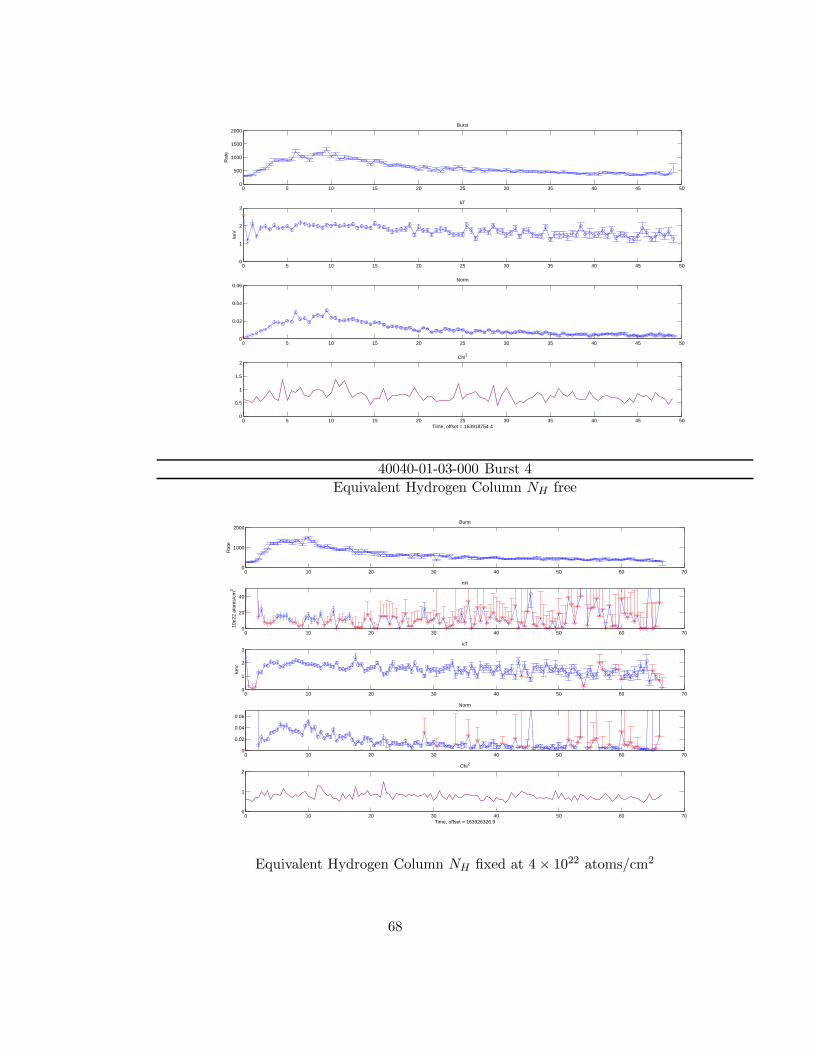
0 5 10 15 20 25 30 35 40 45 500

500

1000

1500

2000Burst

Rat

e

0 5 10 15 20 25 30 35 40 45 500

1

2

3kT

keV

0 5 10 15 20 25 30 35 40 45 500

0.02

0.04

0.06Norm

0 5 10 15 20 25 30 35 40 45 500

0.5

1

1.5

2Chi2

Time, offset = 163918754.4

40040-01-03-000 Burst 4

Equivalent Hydrogen Column NH free

0 10 20 30 40 50 60 700

1000

2000Burst

Rat

e

0 10 20 30 40 50 60 700

20

40

nH

10e2

2 at

oms/

cm2

0 10 20 30 40 50 60 700

1

2

3kT

keV

0 10 20 30 40 50 60 700

0.02

0.04

0.06

Norm

0 10 20 30 40 50 60 700

1

2Chi2

Time, offset = 163926326.9

Equivalent Hydrogen Column NH fixed at 4 × 1022 atoms/cm2

68

0 10 20 30 40 50 60 700

500

1000

1500

2000Burst

Rat

e

0 10 20 30 40 50 60 700

1

2

3kT

keV

0 10 20 30 40 50 60 700

0.02

0.04

0.06Norm

0 10 20 30 40 50 60 700

0.5

1

1.5

2Chi2

Time, offset = 163926326.9

70050-03-01-00 Burst 1

Equivalent Hydrogen Column NH free

0 10 20 30 40 50 600

500

1000

1500Burst

Rat

e

0 10 20 30 40 50 600

10

20

30nH

10e2

2 at

oms/

cm2

0 10 20 30 40 50 600

1

2

3kT

keV

0 10 20 30 40 50 600

0.02

0.04

Norm

0 10 20 30 40 50 600

1

2Chi2

Time, offset = 307120824.9

Equivalent Hydrogen Column NH fixed at 4 × 1022 atoms/cm2

69

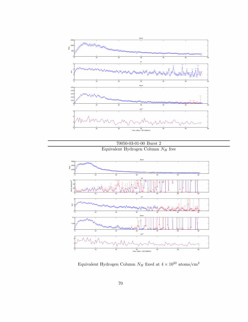
0 10 20 30 40 50 600

500

1000

1500Burst

Rat

e

0 10 20 30 40 50 600

1

2

3kT

keV

0 10 20 30 40 50 600

0.01

0.02

0.03

0.04

0.05Norm

0 10 20 30 40 50 600

1

2

3Chi2

Time, offset = 307120824.9

70050-03-01-00 Burst 2

Equivalent Hydrogen Column NH free

0 10 20 30 40 50 600

1000

2000

3000Burst

Rat

e

0 10 20 30 40 50 600

10

20

30nH

10e2

2 at

oms/

cm2

0 10 20 30 40 50 600

2

4kT

keV

0 10 20 30 40 50 600

0.05

0.1Norm

0 10 20 30 40 50 600

1

2

Chi2

Time, offset = 307130509.9

Equivalent Hydrogen Column NH fixed at 4 × 1022 atoms/cm2

70

0 10 20 30 40 50 600

1000

2000

3000Burst

Rat

e

0 10 20 30 40 50 600

1

2

3

4kT

keV

0 10 20 30 40 50 600

0.02

0.04

0.06

0.08

0.1Norm

0 10 20 30 40 50 600

0.5

1

1.5

2

2.5Chi2

Time, offset = 307130509.9

70050-03-01-01 Burst 1

Equivalent Hydrogen Column NH free

0 10 20 30 40 50 600

500

1000Burst

Rat

e

0 10 20 30 40 50 600

10

20

30nH

10e2

2 at

oms/

cm2

0 10 20 30 40 50 600

1

2

3kT

keV

0 10 20 30 40 50 600

0.02

0.04

Norm

0 10 20 30 40 50 600

1

2

Chi2

Time, offset = 307102335.9

Equivalent Hydrogen Column NH fixed at 4 × 1022 atoms/cm2

71

0 10 20 30 40 50 600

500

1000Burst

Rat

e

0 10 20 30 40 50 600

1

2

3kT

keV

0 10 20 30 40 50 600

0.01

0.02

0.03Norm

0 10 20 30 40 50 600

0.5

1

1.5

2

2.5Chi2

Time, offset = 307102335.9

70050-03-01-02 Burst 1

Equivalent Hydrogen Column NH free

0 5 10 15 20 25 30 35 40 450

500

1000

1500

Burst

Rat

e

0 5 10 15 20 25 30 35 40 450

10

20

30nH

10e2

2 at

oms/

cm2

0 5 10 15 20 25 30 35 40 450

1

2

3kT

keV

0 5 10 15 20 25 30 35 40 450

0.02

0.04

Norm

0 5 10 15 20 25 30 35 40 450

1

2

Chi2

Time, offset = 307143565.9

Equivalent Hydrogen Column NH fixed at 4 × 1022 atoms/cm2

72

0 5 10 15 20 25 30 35 40 450

500

1000

1500

Burst

Rat

e

0 5 10 15 20 25 30 35 40 450

1

2

3kT

keV

0 5 10 15 20 25 30 35 40 450

0.02

0.04

0.06Norm

0 5 10 15 20 25 30 35 40 450

0.5

1

1.5

2

2.5Chi2

Time, offset = 307143565.9

90062-03-01-00 Burst 1

Equivalent Hydrogen Column NH free

0 10 20 30 40 50 60 70 80 90 100 1100

500

1000

1500

Burst

Rat

e

0 10 20 30 40 50 60 70 80 90 100 1100

10

20

30nH

10e2

2 at

oms/

cm2

0 10 20 30 40 50 60 70 80 90 100 1100

1

2

3kT

keV

0 10 20 30 40 50 60 70 80 90 100 1100

0.02

0.04

Norm

0 10 20 30 40 50 60 70 80 90 100 1100

1

2

Chi2

Time, offset = 347061870.9

Equivalent Hydrogen Column NH fixed at 4 × 1022 atoms/cm2

73

0 10 20 30 40 50 60 70 80 90 100 1100

500

1000

1500

Burst

Rat

e

0 10 20 30 40 50 60 70 80 90 100 1100

10

20

30nH

10e2

2 at

oms/

cm2

0 10 20 30 40 50 60 70 80 90 100 1100

1

2

3kT

keV

0 10 20 30 40 50 60 70 80 90 100 1100

0.02

0.04

Norm

0 10 20 30 40 50 60 70 80 90 100 1100

1

2

Chi2

Time, offset = 347061870.9

90062-03-01-010 Burst 1

Equivalent Hydrogen Column NH free

0 10 20 30 40 50 60 70 80 90 1000

500

1000Burst

Rat

e

0 10 20 30 40 50 60 70 80 90 1000

10

20

30nH

10e2

2 at

oms/

cm2

0 10 20 30 40 50 60 70 80 90 1000

1

2

3kT

keV

0 10 20 30 40 50 60 70 80 90 1000

0.01

0.02

0.03Norm

0 10 20 30 40 50 60 70 80 90 1000

1

2

3Chi2

Time, offset = 347083579.9

Equivalent Hydrogen Column NH fixed at 4 × 1022 atoms/cm2

74

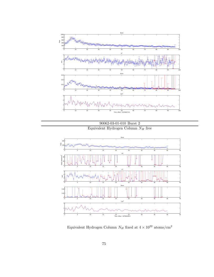
0 10 20 30 40 50 60 70 80 90 1000

200

400

600

800

1000Burst

Rat

e

0 10 20 30 40 50 60 70 80 90 1000

1

2

3kT

keV

0 10 20 30 40 50 60 70 80 90 1000

0.01

0.02

0.03Norm

0 10 20 30 40 50 60 70 80 90 1000

1

2

3Chi2

Time, offset = 347083579.9

90062-03-01-010 Burst 2

Equivalent Hydrogen Column NH free

0 5 10 15 20 25 30 35 40 450

200

400

Burst

Rat

e

0 5 10 15 20 25 30 35 40 450

20

40

nH

10e2

2 at

oms/

cm2

0 5 10 15 20 25 30 35 40 450

1

2

3kT

keV

0 5 10 15 20 25 30 35 40 450

0.02

0.04

Norm

0 5 10 15 20 25 30 35 40 450

1

2Chi2

Time, offset = 347084430.4

Equivalent Hydrogen Column NH fixed at 4 × 1022 atoms/cm2

75

0 5 10 15 20 25 30 35 40 450

100

200

300

400

500Burst

Rat

e

0 5 10 15 20 25 30 35 40 450

1

2

3kT

keV

0 5 10 15 20 25 30 35 40 450

0.002

0.004

0.006

0.008

0.01Norm

0 5 10 15 20 25 30 35 40 450

0.5

1

1.5

2Chi2

Time, offset = 347084430.4

90062-03-01-010 Burst 3

Equivalent Hydrogen Column NH free

0 20 40 60 80 100 1200

500

1000

1500Burst

Rat

e

0 20 40 60 80 100 1200

10

20

30nH

10e2

2 at

oms/

cm2

0 20 40 60 80 100 1200

1

2

3kT

keV

0 20 40 60 80 100 1200

0.01

0.02

0.03Norm

0 20 40 60 80 100 1200

1

2

3

Chi2

Time, offset = 347097644.4

Equivalent Hydrogen Column NH fixed at 4 × 1022 atoms/cm2

76

0 20 40 60 80 100 1200

500

1000

1500Burst

Rat

e

0 20 40 60 80 100 1200

1

2

3kT

keV

0 20 40 60 80 100 1200

0.01

0.02

0.03Norm

0 20 40 60 80 100 1200

1

2

3Chi2

Time, offset = 347097644.4

90062-03-01-010 Burst 4

Equivalent Hydrogen Column NH free

0 10 20 30 40 50 60 70 80 90 100 1100

500

1000

1500Burst

Rat

e

0 10 20 30 40 50 60 70 80 90 100 1100

10

20nH

10e2

2 at

oms/

cm2

0 10 20 30 40 50 60 70 80 90 100 1100

1

2

3kT

keV

0 10 20 30 40 50 60 70 80 90 100 1100

0.01

0.02

0.03Norm

0 10 20 30 40 50 60 70 80 90 100 1100

1

2

3

Chi2

Time, offset = 347108871.9

Equivalent Hydrogen Column NH fixed at 4 × 1022 atoms/cm2

77

0 10 20 30 40 50 60 70 80 90 100 1100

500

1000

1500Burst

Rat

e

0 10 20 30 40 50 60 70 80 90 100 1100

1

2

3kT

keV

0 10 20 30 40 50 60 70 80 90 100 1100

0.01

0.02

0.03Norm

0 10 20 30 40 50 60 70 80 90 100 1100

1

2

3Chi2

Time, offset = 347108871.9

90062-03-01-02 Burst 1

Equivalent Hydrogen Column NH free

0 10 20 30 40 50 60 70 80 90 100 1100

500

1000

1500Burst

Rat

e

0 10 20 30 40 50 60 70 80 90 100 1100

10

20nH

10e2

2 at

oms/

cm2

0 10 20 30 40 50 60 70 80 90 100 1100

1

2

3kT

keV

0 10 20 30 40 50 60 70 80 90 100 1100

0.01

0.02

0.03Norm

0 10 20 30 40 50 60 70 80 90 100 1100

1

2

3

Chi2

Time, offset = 347072631.9

Equivalent Hydrogen Column NH fixed at 4 × 1022 atoms/cm2

78

0 10 20 30 40 50 60 70 80 90 100 1100

500

1000

1500Burst

Rat

e

0 10 20 30 40 50 60 70 80 90 100 1100

1

2

3kT

keV

0 10 20 30 40 50 60 70 80 90 100 1100

0.01

0.02

0.03

0.04

0.05Norm

0 10 20 30 40 50 60 70 80 90 100 1100

1

2

3Chi2

Time, offset = 347072631.9

79

E Crab Soft colour over the years

Soft colour of the Crab versus time for each PCU. The soft colour is definedas 3.5 − 6.0/2.0 − 3.5 keV. Visible in this plot is the gain change per epoch,indicated with the dashed lines. PCU0 lost the propane layer, so the colour(∼1.8) is off the scale. Picture taken from van Straaten, van der Klis &Mendez, 2003.

80

F QPO fits

Here I present the results of the fits made to the power spectra. In Table 8are the results of the fit to the 1-Hz QPO in the range of 0.1−100 Hz with aLorentzian and a power law. It was not possible to fit the observations withObsId=70050. I have discovered a kHz QPO in the combined observationsObsId= 70050-03-01-00 and ObsId=70050-03-01-02. In Table 7 I present theupper limits to the kHz QPO in the other observations (see Section 2.3.1).

Table 7: The kHz QPO has been detected in the observations ObsId=70050-03-01-00 and ObsId=70050-03-01-02. In this table I give the upper limits ofthe fits to the kHz QPO in all data sets except ObsId=70050-03-01-00 andObsId=70050-03-01-02 (see Section 2.3.1).Observation rms 95 %

20066-02-01-00 44.5 %20066-02-01-01 44.8 %20066-02-01-02 30.5 %20066-02-01-03 24.9 %20066-02-01-04 26.6 %

40040-01-01-000 26.7 %40040-01-02-000 37.4 %40040-01-02-01 3.8 %40040-01-03-000 19.6 %

70050-03-01-01 34.4 %

90062-03-01-00 24.0 %90062-03-01-010 95.5 %90062-03-01-02 8.0 %

81

Table 8: Parameters of fits to 1-Hz QPO and power law in the frequency range 0.1-100 Hz. Errors are the quadratic mean ofpositive and negative error.Observation ID Central RMS ampl. FWHM Power law Power law rms%

frequency(Hz) % index (0.001-1 Hz)

20066-02-01-00 0.86 ± 0.008 9.60 ± 0.42 0.24 ± 2.9E-2 0.74 ± 2.1E-2 12.94 ± 0.4320066-02-01-01 0.88 ± 0.008 8.48 ± 0.39 0.17 ± 3.3E-2 0.72 ± 2.1E-2 13.84 ± 0.4020066-02-01-02 0.77 ± 0.007 9.19 ± 0.46 0.18 ± 4.0E-2 0.71 ± 2.4E-2 13.00 ± 0.5220066-02-01-03 0.87 ± 0.001 9.37 ± 0.51 0.24 ± 3.7E-2 0.64 ± 2.9E-2 10.23 ± 0.5520066-02-01-04 0.79 ± 0.012 9.26 ± 0.62 0.22 ± 5.6E-2 0.63 ± 3.3E-2 10.39 ± 0.6340040-01-01-000 1.85 ± 0.021 12.56 ± 0.42 0.78 ± 7.3E-2 0.60 ± 2.2E-2 8.80 ± 0.3640040-01-02-000 0.65 ± 0.006 9.07 ± 0.43 0.15± 4.7E-2 0.72 ± 2.2E-2 14.40 ± 0.5440040-01-02-01 0.61 ± 0.016 8.90 ± 0.54 0.20 ± 4.0E-2 0.67 ± 4.1E-2 10.50 ± 0.7740040-01-03-000 2.60 ± 0.030 12.83 ± 0.46 1.03 ± 0.10 0.62 ± 2.8E-2 8.08 ± 0.3970050-03-01-00 - - - - -70050-03-01-01 - - - - -70050-03-01-02 - - - - -90062-03-01-00 0.79 ± 0.011 6.91 ± 0.56 0.11 ± 6.9E-2 0.64 ± 6.1E-2 11.79 ± 1.1690062-03-01-010 0.75 ± 0.015 9.87± 0.09 0.20 ± 6.1E-2 0.60 ± 4.5E-2 11.26 ± 0.9590062-03-01-02 0.76 ± 0.020 10.42 ± 0.12 0.12 ± 4.0E-2 0.63 ± 9.9E-2 12.46 ± 1.93

82

G Power spectrum fits

Here I present the power spectra of all observations and their best fits (seeSection 2.3). The power spectra have been Poisson subtracted. The modelused for the fit for all observations (except those with ObsId = 70050) isa power law combined with three Lorentzians. For the observations withObsId=70050 the power law is dismissed and a fit is made only with thethree Lorentzians.

Observation number: 20066-02-01-00

Clean spectrum Fitted spectrum

Observation number: 20066-02-01-01

Clean spectrum Fitted spectrum

83

Observation number: 20066-02-01-02

Clean spectrum Fitted spectrum

Observation number: 20066-02-01-03

Clean spectrum Fitted spectrum

84

Observation number: 20066-02-01-04

Clean spectrum Fitted spectrum

Observation number:40040-01-01-000

Clean spectrum Fitted spectrum

85

Observation number:40040-01-02-000

Clean spectrum Fitted spectrum

Observation number:40040-01-02-01

Clean spectrum Fitted spectrum

86

Observation number:40040-01-03-000

Clean spectrum Fitted spectrum

Observation number:70050-03-01-00& 70050-03-01-02

Clean spectrum Fitted spectrum

87

Observation number:70050-03-01-01

Clean spectrum Fitted spectrum

Observation number:90062-03-01-00

Clean spectrum Fitted spectrum

88

Observation number:90062-03-01-010

Clean spectrum Fitted spectrum

Observation number:90062-03-01-02

Clean spectrum Fitted spectrum

89