the natural 3d spiral - technion - electrical …webee.technion.ac.il/~ayellet/ps/11-hararytal.pdfg....

EUROGRAPHICS 2011 / M. Chen and O. Deussen(Guest Editors)

Volume 30 (2011), Number 2

The Natural 3D Spiral

Gur Harary and Ayellet Tal

Technion – Israel Institute of Technology

(a) A tail of a lizard (b) Oliva porphyria (c) A horn of a Big-Horn Sheep

Figure 1: Modeling a variety of logarithmic-spiral structures in fauna. Real images of the objects are shown on the top left.

AbstractLogarithmic spirals are ubiquitous in nature. This paper presents a novel mathematical definition of a 3D loga-rithmic spiral, which provides a proper description of objects found in nature. To motivate our work, we scannedspiral-shaped objects and studied their geometric properties. We consider the extent to which the existing 3D def-initions capture these properties. We identify a property that is shared by the objects we investigated and is notsatisfied by the existing 3D definitions. This leads us to present our definition in which both the radius of curva-ture and the radius of torsion change linearly along the curve. We prove that our spiral satisfies several desirableproperties, including invariance to similarity transformations, smoothness, symmetry, extensibility, and roundness.Finally, we demonstrate the utility of our curves in the modeling of several animal structures.

Categories and Subject Descriptors (according to ACM CCS): I.3.5 [Computer Graphics]: Computational Geometryand Object Modeling—Curve, surface, solid, and object representations

1. Introduction

Nature is rich in spirals [Coo03, Coo79]. They exist in ani-mal and human anatomy – in horns, seashells, muscles, andbones, as well as in botany – in the formation of leaves, flow-ers (sunflower heads), fruit (pineapples, pine cones), and treetrunks. Hurricanes are shaped as spirals. Some bays, suchas the Half-Moon Bay in California, are spirals. Cook alsopoints to the relation between the incidence of spirals in na-ture and their appearance in art and architecture.

It is thus not surprising that spirals have attracted theattention of mathematicians as well as biologists, zoolo-gists, paleontologists, artists, and psychologists. In computergraphics, despite the aspiration to produce natural-lookingmodels, relatively few attempts have been made to model

spirals. This paper focuses on logarithmic spirals – the onesbelieved to characterize many of the natural phenomena de-scribed above [Mos38, d’A42, Hun70].

The 2D logarithmic spiral is defined in four different man-ners [d’A42,Hun70]. A few extensions of the 2D logarithmicspiral to 3D were introduced for modeling seashells [Cor89,Pic89, FMP92]. They were demonstrated to produce somebeautiful seashells. However, we provide evidence that someof these extensions are too restrictive to describe the richnessof spirals in nature, and prove that the other extensions donot hold any 3D definition.

These observations led us to present a different mathemat-ical extension. It requires that both the radius of the curvatureand the radius of the torsion change linearly along the curve.

c© 2010 The Author(s)Journal compilation c© 2010 The Eurographics Association and Blackwell Publishing Ltd.Published by Blackwell Publishing, 9600 Garsington Road, Oxford OX4 2DQ, UK and350 Main Street, Malden, MA 02148, USA.

G. Harary & A. Tal / The Natural 3D Spiral

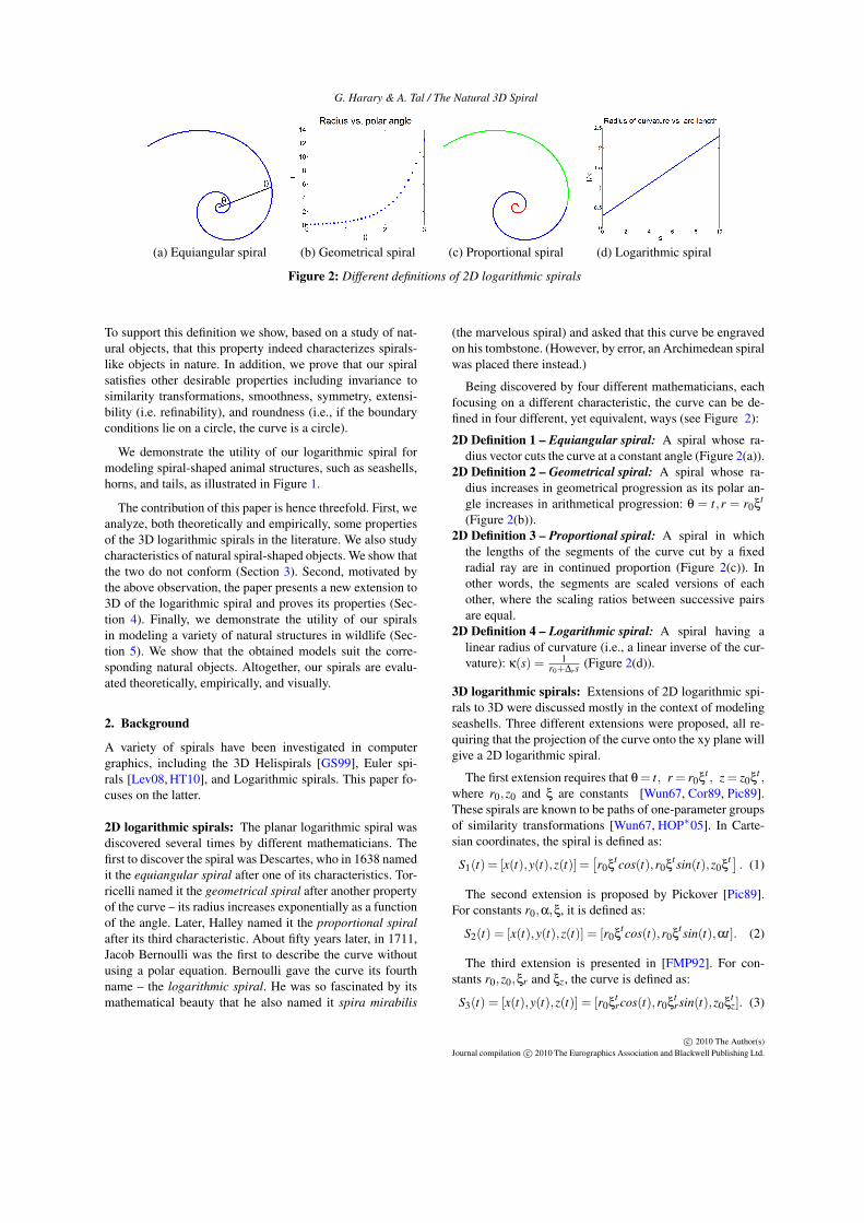
(a) Equiangular spiral (b) Geometrical spiral (c) Proportional spiral (d) Logarithmic spiral

Figure 2: Different definitions of 2D logarithmic spirals

To support this definition we show, based on a study of nat-ural objects, that this property indeed characterizes spirals-like objects in nature. In addition, we prove that our spiralsatisfies other desirable properties including invariance tosimilarity transformations, smoothness, symmetry, extensi-bility (i.e. refinability), and roundness (i.e., if the boundaryconditions lie on a circle, the curve is a circle).

We demonstrate the utility of our logarithmic spiral formodeling spiral-shaped animal structures, such as seashells,horns, and tails, as illustrated in Figure 1.

The contribution of this paper is hence threefold. First, weanalyze, both theoretically and empirically, some propertiesof the 3D logarithmic spirals in the literature. We also studycharacteristics of natural spiral-shaped objects. We show thatthe two do not conform (Section 3). Second, motivated bythe above observation, the paper presents a new extension to3D of the logarithmic spiral and proves its properties (Sec-tion 4). Finally, we demonstrate the utility of our spiralsin modeling a variety of natural structures in wildlife (Sec-tion 5). We show that the obtained models suit the corre-sponding natural objects. Altogether, our spirals are evalu-ated theoretically, empirically, and visually.

2. Background

A variety of spirals have been investigated in computergraphics, including the 3D Helispirals [GS99], Euler spi-rals [Lev08, HT10], and Logarithmic spirals. This paper fo-cuses on the latter.

2D logarithmic spirals: The planar logarithmic spiral wasdiscovered several times by different mathematicians. Thefirst to discover the spiral was Descartes, who in 1638 namedit the equiangular spiral after one of its characteristics. Tor-ricelli named it the geometrical spiral after another propertyof the curve – its radius increases exponentially as a functionof the angle. Later, Halley named it the proportional spiralafter its third characteristic. About fifty years later, in 1711,Jacob Bernoulli was the first to describe the curve withoutusing a polar equation. Bernoulli gave the curve its fourthname – the logarithmic spiral. He was so fascinated by itsmathematical beauty that he also named it spira mirabilis

(the marvelous spiral) and asked that this curve be engravedon his tombstone. (However, by error, an Archimedean spiralwas placed there instead.)

Being discovered by four different mathematicians, eachfocusing on a different characteristic, the curve can be de-fined in four different, yet equivalent, ways (see Figure 2):

2D Definition 1 – Equiangular spiral: A spiral whose ra-dius vector cuts the curve at a constant angle (Figure 2(a)).

2D Definition 2 – Geometrical spiral: A spiral whose ra-dius increases in geometrical progression as its polar an-gle increases in arithmetical progression: θ = t,r = r0ξ

t

(Figure 2(b)).2D Definition 3 – Proportional spiral: A spiral in which

the lengths of the segments of the curve cut by a fixedradial ray are in continued proportion (Figure 2(c)). Inother words, the segments are scaled versions of eachother, where the scaling ratios between successive pairsare equal.

2D Definition 4 – Logarithmic spiral: A spiral having alinear radius of curvature (i.e., a linear inverse of the cur-vature): κ(s) = 1

r0+∆rs (Figure 2(d)).

3D logarithmic spirals: Extensions of 2D logarithmic spi-rals to 3D were discussed mostly in the context of modelingseashells. Three different extensions were proposed, all re-quiring that the projection of the curve onto the xy plane willgive a 2D logarithmic spiral.

The first extension requires that θ = t, r = r0ξt , z = z0ξ

t ,where r0,z0 and ξ are constants [Wun67, Cor89, Pic89].These spirals are known to be paths of one-parameter groupsof similarity transformations [Wun67, HOP∗05]. In Carte-sian coordinates, the spiral is defined as:

S1(t) = [x(t),y(t),z(t)] =[r0ξ

tcos(t),r0ξtsin(t),z0ξ

t] . (1)

The second extension is proposed by Pickover [Pic89].For constants r0,α,ξ, it is defined as:

S2(t) = [x(t),y(t),z(t)] = [r0ξtcos(t),r0ξ

tsin(t),αt]. (2)

The third extension is presented in [FMP92]. For con-stants r0,z0,ξr and ξz, the curve is defined as:

S3(t) = [x(t),y(t),z(t)] = [r0ξtrcos(t),r0ξ

trsin(t),z0ξ

tz]. (3)

c© 2010 The Author(s)Journal compilation c© 2010 The Eurographics Association and Blackwell Publishing Ltd.


(a) Equitangential spiral (b) Geometrical spiral (c) Proportional spiral (d) Logarithmic spiral

Figure 3: Different definitions of 3D logarithmic spirals

(a) Scanned object (b) Ratio curvature / torsion (c) Linear fit to 1/κ (d) Linear fit to 1/τ

Figure 4: Two models out of the eleven natural objects we scanned. The ratios between their radii of torsion and their radii ofcurvature were measured (b). It can be seen that these quantities are not related by scale. The graphs in (c-d) illustrate that theradii of the curvature & torsion, each grows approximately linearly. See additional results in the supplementary material.

Though this extension generalizes the first extension, inpractice, most of the results shown in [FMP92] use a con-strained set of parameters (ξr = ξz = ξ), resulting in curvesthat coincide with those of the first extension.

In the next section we discuss the reasons for the insuffi-ciency of these extensions for modeling some natural loga-rithmic spiral-shaped objects. In light of this discussion wepresent in Section 4 a novel definition.

3. Do previous extensions suffice?

We start by giving four definitions of 3D logarithmic spirals,each extends one of the 2D definitions. We then describeour empirical study in which we examine some propertiesof natural spiral-shaped objects. We consider how well theexisting 3D extensions comply with the 3D definitions andwhether they suit the properties captured in the study. Fi-nally, we identify a property that is shared by the objects weinvestigated and is not satisfied by the known extensions.

3D Definition 1 – Equitangential spiral: A spiral for

which any plane adjacent to the spiral’s major axis cuts itat a constant tangent (Figure 3(a)).

3D Definition 2 – Geometrical spiral: A spiral for whichthe length of the radius R increases in geometrical pro-gression as its polar angle θ increases in arithmetical pro-gression, where R =

√x2 + y2 + z2 and θ = arctan(y/x)

(Figure 3(b)).3D Definition 3 – Proportional spiral: A spiral for which

the lengths of the segments of the curve, cut by a planethrough the spiral’s major axis, are in continued propor-tion (Figure 3(c)).

3D Definition 4 – Logarithmic spiral: A spiral having alinear radius of curvature and a linear radius of torsion(Figure 3(d)).

In our study, we scanned eleven seashells, horns, and fruit.Figure 4(a) shows a couple of the scanned objects. We thencomputed the change in the radius of the curvature ( 1

κ) and

that of the radius of the torsion ( 1τ) for curves on the ob-

jects’ surfaces. These curves are the smoothed valleys andridges of the surface. The curvature and the torsion were



computed using the independent coordinates method pro-posed by [LGLC05], which is shown to be robust to noise.

The beauty of the first 3D extension (S1, Equation (1)) isthat it satisfies all four 3D definitions. However, we prove inAppendix A (Proposition A.1) that in this spiral the radius ofcurvature and the radius of torsion are equal up to a constant(i.e. it is a curve of constant slope). But, our study shows thatthis is not the case in nature – the radii are not related by anyconstant; see Figure 4(b). Like any other general 3D curve,the curvature and the torsion are independent. Hence, spi-rals that relate them are too restrictive and cannot accuratelydescribe the variety of natural spiral objects.

We now turn to examine S2 and S3 (Equations (2)–(3)).We prove in Appendix A (Propositions A.2–5) that these spi-rals do not satisfy any of the above 3D definitions. Hence,while they produce pretty results, theoretically they are notproper extensions. Moreover, we later demonstrate in Fig-ure 6 that these spirals are indeed less accurate for describingnatural objects than our spiral.

Finally, our study also shows that linear radii of the cur-vature and torsion approximately characterize the curves, inaccordance with 3D Definition 4; see Figures 4(c-d). Thiscalls for a different mathematical extension of a logarithmicspiral – one that satisfies this definition. This is the rationalebehind our definition, which is discussed next.

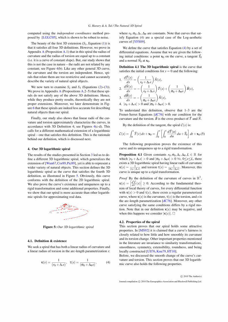
4. Our 3D logarithmic spiral

The results of the studies presented in Section 3 led us to de-fine a different 3D logarithmic spiral, which generalizes theextension of [Wun67,Cor89,Pic89], yet is able to represent awider variety of natural objects. This section defines the 3Dlogarithmic spiral as the curve that satisfies the fourth 3Ddefinition, as illustrated in Figure 5. Obviously, this curveconforms with the definition of the 2D logarithmic spiral.We also prove the curve’s existence and uniqueness up to arigid transformation and some additional properties. Finally,we show that our spiral is more accurate than other logarith-mic spirals for approximating real data.

Figure 5: Our 3D logarithmic spiral

4.1. Definition & existence

We seek a spiral that has both a linear radius of curvature anda linear radius of torsion in the arc-length parametrization s:

κ(s) =1

(r0 +∆rs), τ(s) =

1(σ0 +∆σs)

, (4)

where r0,σ0,∆r,∆σ are constants. Note that curves that sat-isfy Equation (4) are a special case of the Log-aestheticcurves of [YFS09].

We define the curve that satisfies Equation (4) by a set ofdifferential equations. Assume that we are given the follow-ing initial conditions: a point x0 on the curve, a tangent ~T0and a normal ~N0 at x0.

Definition 4.1 The 3D logarithmic spiral is the curve thatsatisfies the initial conditions for s = 0 and the following:

1.d~T (s)

ds=

(1

r0 +∆rs

)~N(s),

2.d~N(s)

ds=−

(1

r0 +∆rs

)~T (s)+

(1

σ0 +∆σs

)~B(s),

3.d~B(s)

ds=−

(1

σ0 +∆σs

)~N(s),

4. |r0 +∆rs|> 0 and |σ0 +∆σs|> 0.

To understand this definition, observe that 1–3 are theFrenet-Serret Equations [dC76] with our condition for thecurvature and the torsion. ~B is the cross product of ~T and ~N.

By the definition of the tangent, the spiral C(s) is:

C(s) =∫ s

0~T (v)dv+x0 =

∫ s

0

[∫ t

0

d~T (u)du

du+~T0

]dt +x0.(5)

The following proposition proves the existence of thiscurve and its uniqueness up to a rigid transformation.

Proposition 4.1 Given constants r0,σ0,∆r,∆σ,L ∈ R forwhich |r0 +∆rs| > 0 and |σ0 +∆σs| > 0 ∀s, 0≤s≤L, thereexists a 3D logarithmic spiral having linear radii of curvatureκ(s) = 1

(r0+∆rs) and torsion τ(s) = 1(σ0+∆σs) . Moreover, this

curve is unique up to a rigid transformation.

Proof By the definition of the curvature of curves in R3,κ(s) =

∣∣∣ d2~Cds2 (s)

∣∣∣ ≥ 0. According to the fundamental theo-rem of local theory of curves, for every differential functionwith κ(s) > 0 and τ(s), there exists a regular parameterizedcurve, where κ(s) is the curvature, τ(s) is the torsion, and s isthe arc-length parametrization [dC76]. Moreover, any othercurve satisfying the same conditions differs by a rigid mo-tion. Note that in our definition κ(s) may be negative, andwhen this happens we consider |κ(s)|. �

4.2. Properties of the spiralThis section proves that our spiral holds some attractiveproperties. In [MS92] it is claimed that a curve’s fairness isclosely related to how little and how smoothly its curvatureand its torsion change. Other important properties mentionedin the literature are invariance to similarity transformations,smoothness, symmetry, extensibility, roundness, and beinglocally constructed [Ull76, Knu79, HT10].Before, we discussed the smooth change of the curve’s cur-vature and torsion. This section proves that our 3D logarith-mic curve also holds the following properties.

c© 2010 The Author(s)

Journal compilation c© 2010 The Eurographics Association and Blackwell Publishing Ltd.


1. Invariance to similarity transformations – translation, ro-tation, and scale. For the latter, we show that scaling ofthe end-points scales the curve by the same scaling factor.

2. Smoothness: The tangent is defined at every point, i.e.,∂C∂s is finite. (In fact, our curve is C∞-smooth.)

3. Symmetry: The curve leaving the point x0 with tangent~T0 and reaching the point x f with tangent ~Tf , coincideswith the curve leaving the point x f with tangent−~Tf andreaching the point x0 with tangent −~T0.

4. Extensibility: For every point xm ∈ C between the end-points x0 and x f , the curves C1 (between x0 and xm) andC2 (between xm and x f ) coincide with C.

5. Roundness: If C interpolates two point-tangent pairs ly-ing on a circle, then C is a circle.

Proposition 4.2 A 3D logarithmic spiral is invariant to sim-ilarity transformations.

Proof Invariance to rotation and translation results fromProposition 4.1. We next prove scale invariance. We aregiven a logarithmic spiral C of length L, which interpo-lates x0 = C(0) and x f = C(L), and whose parameters arer0,σ0,∆r,∆σ. We should show that the spiral Cλ, whichinterpolates λx0 and λx f for λ > 0, is equal to λC, i.e.,∀s,0≤ s≤ L Cλ(s) = λC(s). Thus, we need to find the con-stants r0, σ0, ∆r, ∆σ, L that define the logarithmic spiral Cλ,for which Cλ(0) = λx0 and Cλ(λL) = λx f , with tangents ~T0

and ~Tf respectively. Then, we should show that every pointon this curve coincides with λC.It easy to show that the 3D logarithmic spiral having param-eters r0 = λr0, σ0 = λσ0, ∆r = ∆r, ∆σ = ∆σ, L = λL is thesought-after curve.This is done by substituting these parameters in Defini-tion 4.1(1–3) and defining a new parameter v= s/λ (⇒ dv=ds/λ). We get that d~T

ds = d~Tdv

dvds =

1λ

d~Tdv . Similarly, d~N

ds = 1λ

d~Ndv

and d~Bds = 1

λ

d~Bdv . Hence, this curve satisfies Definition 4.1

with parameter v.We can now calculate the 3D logarithmic spiral as follows:

~Tλ(s) =∫ λs

0

d~Tdu

du+~T0

v=u/λ=

∫ s

0

1λ

d~Tdv

λdv+~T0 = ~T (s),

Cλ(s) =∫ λs

0

[∫ t

0

d~Tdu

du+ ~T0

]dt +λx0

v=u/λ=

∫ λs

0

[∫ t/λ

0

1λ

d~Tdv

λdv+ ~T0

]dt +λx0

t=t/λ=

∫ s

0

[∫ t

0

d~Tdv

dv+ ~T0

]λdt +λx0 = λC(s).

This holds for every 0≤s≤L. As a special case, we get theboundary conditions Cλ(0) = λC(0) = λx0, ~Tλ(0) = ~T (0) =~T0 and Cλ(λL) = λC(L) = λx f , ~Tλ(λL) = ~T (L) = ~Tf . �

Proposition 4.3 A 3D logarithmic spiral is smooth.

Proof According to Proposition 4.1, there exists a solutionfor the Frenet-Serret equations. Therefore, ∂C

∂s = ~T (s) is de-fined for every 0≤s≤L. �

Proposition 4.4 A 3D logarithmic spiral is symmetric.

Proposition 4.5 A 3D logarithmic spiral is extensible.

The proofs of propositions 4.4–4.5 are given in appendix B.

Proposition 4.6 A 3D logarithmic spiral is round.

Proof For given two point-tangent pairs lying on a circle,the circle defined by r0 6= 0,σ0 →∞,∆r = 0,∆σ = 0 is asolution of the Frenet-Serret Equations.�

4.3. ResultsTo verify the suitability of our spiral for describing natu-ral objects, we compared it, as well as the other proposedspirals (S1,S2,S3), to the spirals obtained from our scannedobjects (Figure 4). This is done as follows. Given a scannedobject, its main axis is found [HOP∗05] (this step is neededonly for S2 and S3). Then, depending on the spiral defini-tion, the values of the free parameter (arc-length s for ourspiral and angle t for the other spirals) at sampled points, arefound. Next, the alignment between the curves is calculatedusing [MHTG05]. Finally, the mean-square error (MSE)between the spiral of the scanned object and that of theanalytically-computed spiral is computed using a Gradient-Descent algorithm that minimizes this error.Figure 6 displays some of the results for the normalized ob-jects. It can be seen that our spiral better fits the data thanthe other spirals and that our error is smaller. We performcomparisons to two out of three previous logarithmic spiralssince S3 includes S1 as a special case. Thus, in essence, wecompared our results to all previous spirals.

S2 S3 Our spiral MSES2: 5.7E-3

S3: 1.4E-3

Ours: 0.85E-3

S2: 0.77E-3

S3: 1.6E-3

Ours: 0.21E-3

Figure 6: Fitting the different spirals (red) to the spirals ofthe real data (blue) in Figure 4(a). Top: seashell, bottom:pine cone. Right: the error obtained by fitting the spirals.See additional results in the supplementary material.

5. Application: Modeling spiral-like structures in faunaThis section presents our results for modeling seashells,horns, and other animal structures – all believed to complywith the logarithmic structure.

Modeling seashells: The beauty of seashells has attractedthe attention of many researchers. Moseley [Mos38] was



the first to characterize seashells with logarithmic spi-rals. His characteristic was supported experimentally byd’Arcy [d’A42]. Raup [Rau61, Rau62] proposed to modelthe morphology of a shell. In computer graphics, enhancedappearance of shell models was suggested by [Kaw82,Opp86, PS86]. Increased attention to details was presentedin [Ill87, Cor89]. Fowler et al. [FMP92] extended the mor-phological model of [Cor89] and added a pigmentation pat-tern to the model, which together resulted in pretty seashells.Our modeling algorithm follows [FMP92]. Therefore, wepresent it only briefly, for the sake of completeness of thedescription. The main difference between the algorithms isthe use of our spiral to model the seashells instead of S3. Wealso address the issue of shell opening, which has not beenhandled previously.The algorithm, illustrated in Figure 7, has four steps: First,a 3D logarithmic spiral is constructed. Then, the shell’s sur-face is constructed. Third, the shell’s opening is formed, andfinally the shell’s pattern is generated.

(a) Spiral (b) Surface (c) Opening (d) Pigmentation

Figure 7: Algorithm outline

1. 3D LOGARITHMIC SPIRAL CONSTRUCTION: A 3D log-arithmic spiral Clog is constructed. This is done by simplychoosing the curve’s parameters r0,σ0,∆r,∆σ and L, and ap-proximating Clog numerically using the Runge-Kutta 5 (4)method [DP80]. This is an adaptive one-step solver, in whichthe computation of the point x(tn+1) needs only the solutionat the immediately preceding time point x(tn). It is designedto produce an estimate of the local truncation error of a sin-gle Runge-Kutta step, and as result, allows to control theerror with an adaptive step-size. That is done by having twoRunge-Kutta methods, one with order 5 and one with order4. This is to say, the total accumulated error has order h5

(respectively, h4), where h is a basic, non-adaptive step-sizeof t. In practice, we used 250 sample points for the curvesin our models. We examined the MSE between these curvesand denser curves with 10000 sample points. The averageMSE is 1.6E-4.

2. SHELL SURFACE CONSTRUCTION: The surface is built asa general sweep surface, where Clog is the route. In practice,Clog is sampled and a closed curve – the generating curve– traverses only the sampled points. The generating curve isscaled along the route linearly w.r.t. the arc-length of the spi-ral. The resulting surface is represented by a mesh, where a

(a) Real seashell (b) [FMP92] (c) Our result

Figure 8: Turrirella nivea. Our result is similar to the nat-ural Turrirella nivea in width, in the number of revolutions,in the height of each revolution, and in the opening.


Figure 9: Papery rapa. Our model captures the generalshape as well as the upper tip of the shell and the opening.

triangle strip is built between every pair of consecutive gen-erating curves.

3. FORMING THE SHELL OPENING: The sweeping of auniformly growing generating curve along the logarithmicspiral produces a strictly self-similar surface that can bemapped onto itself by scale and rotation around the shellaxis [d’A42]. In real shells, the lips at the shell opening oftendisplay a departure from self-similarity.We model the opening using a closed curve Copen that de-scribes the shape of the opening. Instead of sweeping thegenerating curve along the entire logarithmic spiral as donein [FMP92], we sweep it only when the parameter s isin the range [s0,L− ∆L]. For the rest of the spiral, whens ∈ [L− ∆L,L], we use a linear interpolation between thegenerating curve and Copen.

4. PIGMENTATION PATTERN GENERATION: Pigmentationpatterns in shells show an enormous amount of diversity. Wesimulate them using a class of reaction-diffusion models de-veloped by [MK87a, MK87b] and used in [FMP92]. For agiven biological model, described by reaction-diffusion dif-ferential equations, the solution results in an image, which ismapped to the mesh.

RESULTS: Figures 8–11 illustrate some results obtained byour algorithm. These examples were chosen since they weremodeled by [FMP92], and thus they allow us to provide a





Figure 10: Conus marmoreus. Our spiral yields better mod-eling of the top and bottom tips, as well as a better opening.


Figure 11: Oliva porphyria. Note the tips and opening.

fair comparison to the results presented in their paper as wellas to the original images given there. Since the seashellsof [FMP92] were produced by a constrained spiral model(S1 is a special case of S3), these comparisons can be viewedalso as comparisons to S1.Our models are more similar to the natural seashells in sev-eral manners. First, as our spiral is less restrictive, we areable to produce seashells whose general structure better re-sembles the natural shells than its competitors (Figures 8–9).Second, the upper and the lower tips of our shells look morenatural (Figures 9–10). Finally, since we added opening for-mation, we are able to control it and produce narrower orwider openings, as required (Figures 10–11). The last twosteps of the algorithm – opening formation and pigmenta-tion – were applied only to the models in Figures 10–11.

Modeling horns: Animal horns are structured as logarith-mic spirals [d’A42]. Yet, there exist only a few studies thatmodel horns. In [Kaw82, Ste09] a horn is created by assem-bling given modules along a path. In [Kaw82] every branchof the horn is a 2D spiral, whereas in [Ste09] the path is S3.We propose to model the geometry of horns in two steps.First, the 3D logarithmic spiral is constructed. Then, asurface that supports 3D texture (i.e. fluctuations) is con-structed, in compliance with the fact that horns have visible3D textures. We propose to create this structure by addingsmall fluctuations to the size of the generating curve whentraversed along the route Clog. The fluctuations can be re-

(a) Image of an Ibex (b) Our model

Figure 12: Horn of an Ibex. Note the outer fluctuations.

(a) Image of an Impala (b) Our model

Figure 13: Horn of an Impala. Note the bending of the horn.

(a) Image of a Kudu (b) [Ste09] (c) Our model

Figure 14: Horn of a Kudu. Note the twisting.

stricted to only part of the generating curve, as illustrated inFigures 1(c),12,14, where only the “outer” part of the hornshas fluctuations.The provided results demonstrate not only the 3D fluctua-tion, but also the ability of our algorithm to support bending(curvature), as demonstrated in Figure 12, and twisting (tor-sion), shown in Figures 1(c) and 14. Figure 14 also showsthe modeling of the Kudu’s horn in [Ste09]. (The paper doesnot provide the image this model is inspired by.)

Modeling other animal structures: A variety of other or-gans of animals are shaped as logarithmic spirals. Figure 15shows our model of a cochlea, which is the auditory portionof the inner ear. It is a spiralled, hollow, conical chamber ofbone. Figures 1(a) and 16 show our models of spiral-shapedtails – that of a lizard and that of a sea horse. In all theseexamples, our models resemble the spirals in the images. InFigure 1(a), the mesh was textured using standard texturemapping.



(a) Image of a cochlea (b) Our model

Figure 15: Cochlea

(a) Image of a sea horse (b) Our tail model

Figure 16: Sea horse tail

Running time and user interaction: The algorithm wasimplemented in Matlab and ran on a 2Ghz Intel Core 2 Due-processor machine with 2Gb of memory. The running timeis about 5 seconds for a 100,000-vertex model.We built a GUI that allows the user to control the parame-ters. The user’s interaction is similar to that of the previousapproaches – requiring to choose a similar number of pa-rameters. Table 1 lists the parameters used for generatingthe models presented in this paper.

Figure r0 ∆r σ0 ∆σ L1(a),11 1 0.2 10 1 57

1(b) 5E-4 0.03 0.1 0.85 0.41(c) 0.6 0.1 2 15 5.2

8 0.002 0.025 0.1 0.02 2.69 0.008 0.1 10 10 11

10 0.005 0.03 0.2 1.25 512 1 0.2 1 1 813 0.1 0.5 0.1 1.2 3.514 0.01 0.01 3 5 0.1215 0.005 0.115 0.4 0.4 2.316 1.75E-3 0.19 0.2 0.2 0.12

Table 1: Parameters of the models presented in the paper

Limitations: Our modeling technique cannot model largespikes and extrusions, which exist in some seashells,e.g., Figure 4 (top). In addition, it cannot handle distortions

in the model, such as the one shown at the bottom tip of theshell in Figure 9(a).

6. ConclusionLogarithmic spirals characterize many natural structures.This paper addressed the challenge of extending the well-known 2D logarithmic spiral to 3D. Our mathematical def-inition was motivated by studying previous extensions andshowing that they may be too restrictive for representing thevariety of spiral-shaped objects.We provide three types of analysis of our spirals as well as ofpreviously proposed spirals: theoretical, empirical, and vi-sual. Theoretically, we prove some desirable properties ofthe spiral. Empirically, we scanned objects and tested the fitbetween the mathematical definitions and actual spirals innature. Visually, we produced models that demonstrate theuse of the various spirals for modeling structures that appearin the wildlife. Our spirals outperform the other spirals in allthese aspects.

Acknowledgements This research was supported in part bythe Israel Science Foundation (ISF) 628/08 and by the Ollen-dorff Foundation.

References[Coo03] COOK T.: Spirals in nature and art. Nature 68 (1903),

296. 1

[Coo79] COOK T.: The curves of life. Dover, 1979. 1

[Cor89] CORTIE M.: Models for mollusc shell shape. SouthAfrican Journal of Science 85 (1989), 454–460. 1, 2, 4, 6

[d’A42] D’ARCY W.: On growth and form. Cambridge Univ.Press, 1942. 1, 6, 7

[dC76] DO CARMO M.: Differential geometry of curves and sur-faces. Prentice Hall, 1976. 4, 9

[DP80] DORMAND J., PRINCE P.: A family of embedded Runge-Kutta formulae. Journal of Computational and Applied Mathe-matics 6, 1 (1980), 19–26. 6

[FMP92] FOWLER D., MEINHARDT H., PRUSINKIEWICZ P.:Modeling seashells. ACM Trans. Graph. 26, 2 (1992), 379–387.1, 2, 3, 6, 7, 9, 10

[GS99] GLAESER G., STACHEL H.: Open geometry: OpenGL+advanced geometry. Springer Verlag, 1999. 2

[HOP∗05] HOFER M., ODEHNAL B., POTTMANN H., STEINERT., WALLNER J.: 3D shape recognition and reconstruction basedon line element geometry. In ICCV (2005), vol. 2, pp. 1532–1538. 2, 5

[HT10] HARARY G., TAL A.: 3D Euler spirals for 3D curve com-pletion. In ACM Symp. on Comp. Geometry (2010). 2, 4

[Hun70] HUNTLEY H.: The divine proportion: A study in mathe-matical beauty. Dover, 1970. 1

[Ill87] ILLERT C.: Formulation and solution of the classicalseashell problem. Il Nuovo Cimento D 9, 7 (1987), 791–814.6

[Kaw82] KAWAGUCHI Y.: A morphological study of the form ofnature. SIGGRAPH 16, 3 (1982), 223–232. 6, 7

[Knu79] KNUTH D.: Mathematical typography. American Math-ematical Society 1, 2 (1979), 337–372. 4




[Lev08] LEVIEN R.: The Euler spiral: a mathematical history.Tech. Rep. UCB/EECS-2008-111, UC, Berkeley, 2008. 2

[LGLC05] LEWINER T., GOMES J., LOPES H., CRAIZER M.:Curvature and torsion estimators based on parametric curve fit-ting. Computers & Graphics 29, 5 (2005), 641–655. 4

[MHTG05] MÜLLER M., HEIDELBERGER B., TESCHNER M.,GROSS M.: Meshless deformations based on shape matching.ACM Trans. on Graphics 24, 3 (2005), 471–478. 5

[MK87a] MEINHARDT H., KLINGLER M.: A model for patternformation on the shells of molluscs. Journal of Theoretical Biol-ogy 126, 63 (1987), 63–89. 6

[MK87b] MEINHARDT H., KLINGLER M.: Pattern formation bycoupled oscillations: The pigmentation patterns on the shells ofmolluscs. Lecture notes in biomath., 71 (1987), 184–198. 6

[Mos38] MOSELEY H.: On the geometrical forms of turbinatedand discoid shells. Philosophical Trans. of the Royal Society ofLondon 128 (1838), 351–370. 1, 5

[MS92] MORETON H., SÉQUIN C.: Functional optimization forfair surface design. SIGGRAPH 26, 2 (1992), 167–176. 4

[Opp86] OPPENHEIMER P.: Real time design and animation offractal plants and trees. SIGGRAPH 20, 4 (1986), 55–64. 6

[Pic89] PICKOVER C.: A short recipe for seashell synthesis. IEEEComp. Grap. and Applications 9, 6 (1989), 8–11. 1, 2, 4, 9, 10

[PS86] PRUSINKIEWICZ P., STREIBEL D.: Constraint-basedmodeling of three-dimensional shapes. In Graphics Interface(1986), pp. 158–163. 6

[Rau61] RAUP D.: The geometry of coiling in gastropods. Proc.of the National Academy of Sciences of the USA 47, 4 (1961),602–609. 6

[Rau62] RAUP D.: Computer as aid in describing form in gastro-pod shells. Science 138 (1962), 150–152. 6

[Ste09] STEPIEN C.: An IFS-based method for modeling horns,seashells and other natural forms. Computers & Graphics 33, 4(2009), 576–581. 7

[Ull76] ULLMAN S.: Filling-in the gaps: The shape of subjectivecontours and a model for their generation. Biological Cybernetics25, 1 (1976), 1–6. 4

[Wun67] WUNDERLICH W.: Darstellende Geometrie, vol. 2. Bib-liographisches Institut, 1967. 2, 4

[YFS09] YOSHIDA N., FUKUDA R., SAITO T.: Log-aestheticspace curve segments. In SPM (2009), pp. 35–46. 4

Appendix A: S1,S2, S3 and the 3D definitionsThis section discusses the properties of the existing 3D spiralextensions S1,S2,S3 (Equations (1)–(3)).

Proposition A.1 S1 is a curve of constant slope.

Proof: The curvature and the torsion of the spiral S1 are cal-culated as [dC76]:

κ(t) =|S′1(t)×S′′1 (t)||S′1(t)|3

=r0√

1+ ln2(ξ)

ξt [(r20 + z2

0)ln2(ξ)+ r2

0],

τ(t) =(S′1(t)×S′′1 (t))·S′′′1 (t)|S′1(t)×S′′1 (t)|2

=z0ln(ξ)

ξt [(r20 + z2

0)ln2(ξ)+ r2

0].

Thus, the spiral has a constant slope:

τ(t)κ(t)

=

(z0ln(ξ)

r0√

1+ ln2(ξ)

). �

Hereafter we prove that S2,S3 (Equations (2)–(3)) do not sat-isfy any of the four 3D Definitions. We first prove that 3DDefinition 1 is violated in the general case. Then we prove,by providing counter examples, that 3D Definitions 2-4 areviolated. In these examples, the parameters used are r0 =1,α = 3,ξ = 1.1 for S2 and r0 = 1,z0 = 3,ξr = 1.1,ξz = 1.5for S3.

Proposition A.2 S2 and S3 are not equitangential spirals.

Proof: According to 3D Definition 1, the tangents to thecurve at points having polar angles tn = t0 + 2πn (n ∈ N)should be equal, thus they should not depend on n.But, in S2 the tangent is:

T2(tn) = [r0ξtn(ln(ξ)cos(t0)− sin(t0)),

r0ξtn(ln(ξ)sin(t0)+ cos(t0)),α]/‖T2‖,

where ‖T2‖ =√

r20ξ2tn(1+ ln2(ξ))+α2, whereas in S3 the

tangent is:

T3(tn) = [r0ξtnr (ln(ξr)cos(t0)− sin(t0)),

r0ξtnr (ln(ξr)sin(t0)+ cos(t0)),z0ln(ξz)ξ

tnz ]/‖T3‖,

where ‖T3‖=√

r20ξ

2tnr (1+ ln2(ξr))+ z2

0ξ2tnz ln2(ξz).

Hence, in both cases the tangents depend on n. �

Proposition A.3 S2 and S3 are not geometrical spirals.

Proof: According to 3D Definition 2, the length of the ra-dius should depend exponentially on the polar angle, thusthe graph of log(R) w.r.t the polar angle should be linear.Figure 17 demonstrates that for the above counter-examples,the graphs of these spirals are not linear. �

(a) S2 [Pic89] (b) S3 [FMP92]

Figure 17: log(R) vs. t for the parameters specified above

Proposition A.4 S2 and S3 are not proportional spirals.

Proof: According to 3D Definition 3, the ratio between thelength of the radii at the polar angles t1 = t0 and t2 =t0 +2πn for t0 ∈ [0,2π] and n ∈ N should be constant, hence

R(t0)R(t0+2πn) = const, ∀t0 ∈ [0,2π].

Figure 18 shows a counter example for t0 =0,π/8,π/4,3π/8,π/2 and n = 1. It shows that in bothcases the 3D definition does not hold. �

Proposition A.5 S2 and S3 are not logarithmic spirals.

Proof: Figure 19 presents the radius of the curvature and theradius of the torsion for S2 and S3 for the counter example



(a) S2 [Pic89] (b) S3 [FMP92]

Figure 18: R(t0)R(t0+2π)

vs. t0

(a) S2 [Pic89] (b) S3 [FMP92]

Figure 19: Radii of the curvature and torsion as a functionof s.

whose parameters are specified above. As can be seen, bothdo not satisfy 3D Definition 4. �

Appendix B: Proofs of properties of our spiralProposition 4.4 A 3D logarithmic spiral is symmetric.

Proof: Given a 3D logarithmic spiral C that interpolatesthe point-tangent pairs (x0,~T0) and (x f ,~Tf ), we need toshow that the 3D logarithmic spiral Csym that interpolates(x f ,−~Tf ) and (x0,−~T0) coincides with C.Suppose that the parameters of C are r0,σ0,∆r,∆σ,L. Weshow below that the 3D logarithmic spiral Csym whose pa-rameters are r0 = r0 + ∆rL, σ0 = σ0 + ∆σL, ∆r = −∆r,∆σ = −∆σ, L = L, coincides with C and that their tangentsare opposite. According to Definition 4.1 we get:

d~TCsym (s)ds =

(1

r0+∆rL−∆rs

)~NCsym(s),

d~NCsym (s)ds = −

(1

r0+∆rL−∆rs

)~TCsym(s)

+(

1σ0+∆σL−∆σs

)~BCsym(s),

d~BCsym (s)ds = −

(1

σ0+∆σL−∆σs

)~NCsym(s).

By defining a new parameter v = L− s (⇒ dv = −ds),

we get thatd~TCsym

ds =d~TCsym

dvdvds = − d~TCsym

dv = d~TCdv . Similarly,

d~NCsymds = − d~NCsym

dv andd~BCsym

ds = − d~BCsymdv . By the tangent

definition we get:

~TCsym(L− s) =∫ L−s

0d~TCsym

du du−~Tfv=L−u=

∫ sL

d~TCsymdv dv− ~Tf =

∫ Ls

d~TCdv dv−

(∫ L0

d~TCdv dv+~T0

)=−

∫ s0

d~TCdv dv−~T0 =−~TC(s).

We now show that the curve Csym coincides with the curve C:

Csym(L− s) = x f +∫ L−s

0

[∫ t0

d~TCsymdu du−~Tf

]dt

v=L−u= x f +

∫ L−s0

[∫ L−tL

d~TCsymdv dv−~Tf

]dt

t=L−t= x f −

∫ sL

[∫ Lt

d~TCdv dv−~Tf

]dt

= x0 +∫ s

0

[∫ t0

d~TCdv dv+~T0

]dt

Eq. (5)= C(s). �

Proposition 4.5 A 3D logarithmic spiral is extensible.

Proof: Given a 3D logarithmic spiral C that interpolates thepoint-tangent pairs (x0, ~T0) and (x f , ~Tf ), we will show thatfor every (xm, ~Tm) on C, the curves C1 between x0 and xmand C2 between xm and x f coincide with C.Assume that C has parameters r0,σ0,∆r,∆σ,L. Let L1 be thelength of the sub-curve of C from x0 to xm. By the tangentdefinition and by Equation (5):

~Tm =∫ L1

0d~Tdu du+ ~T0, (6)

xm =∫ L1

0

[∫ t0

d~Tdu du+ ~T0

]dt +x0. (7)

By the uniqueness of the curve (Proposition 4.1), C1 withthe parameters r0 = r0, σ0 = σ0, ∆r = ∆r, ∆σ = ∆σ, L = L1,coincides with C for 0≤s≤L1.Next, we show that C2 with the parameters r0 = r0 +∆rL1, σ0 = σ0 + ∆σL1, ∆r = ∆r, ∆σ = ∆σ, L = L− L1, co-incides with C for L1≤s≤L. Let us denote the tangent of thecurve C at C(s) by ~TC(s) and the tangent of the curve C2at C2(s) by ~TC2(s). We need to show that C2 that starts at(xm, ~Tm) reaches C(s) with tangent ~TC(s), ∀s, L1≤s≤L.Similarly to the proof of Proposition 4.4, it can be shownthat ∀s,L1 ≤ s≤ L, the tangent at C2(s−L1) is ~TC(s):

~TC2(s−L1) =∫ s−L1

0d~TC2

du du+ ~Tmv=u+L1=

∫ sL1

d~TCdv dv+ ~Tm

=∫ s

L1

d~TCdv dv+

∫ L10

d~TCdv dv+ ~T0 =

∫ s0

d~TCdv dv+ ~T0 = ~TC(s).

Next, we show that ∀s,L1 ≤ s≤ L, C2(s−L1) = C(s):

C2(s−L1) = xm +∫ s−L1

0

[∫ t0

d~TC2du du+ ~Tm

]dt

v=u+L1= xm +∫ s−L1

0

[∫ t+L1L1

d~TCdv dv+~Tm

]dt

t=t+L1= xm +∫ s

L1

[∫ tL1

d~TCdv dv+~Tm

]dt

= x0 +∫ L1

0

[∫ t0

d~TCdv dv+~T0

]dt +

∫ sL1

[∫ tL1

d~TCdv dv+~Tm

]dt

Eq. (7)= x0 +

∫ L10

[∫ t0

d~TCdv dv+~T0

]dt +

∫ sL1

[∫ t0

d~TCdv dv+~T0

]dt

Eq. (6)= x0 +

∫ s0

[∫ t0

d~TCdv dv+~T0

]dt

Eq. (5)= C(s).�



the natural 3d spiral - technion - electrical …webee.technion.ac.il/~ayellet/ps/11-hararytal.pdfg....

Documents